economic forecasting with an agent-based model
TRANSCRIPT

INSTITUTE FOR ECOLOGICAL ECONOMICS
Economic Forecasting with an
Agent-Based Model
Sebastian Poledna1 Michael Miess2
1International Institute for Advanced Systems Analysis (IIASA), Laxenburg
2Institute for Ecological Economics, WU WienInstitut für Höhere Studien (IHS), Wien
International Institute for Advanced Systems Analysis (IIASA), Laxenburg
Presentation at WIFO Research Seminar
March 3rd, 2020
1 / 43

INSTITUTE FOR ECOLOGICAL ECONOMICS
Outline of presentation
1. Introduction: research questions and overarching ideas.
2. Short introduction into agent-based models (ABMs).
3. Short critique of ABM literature.
4. Development of novel estimated ABM framework validated by economicforecasting:I �Economic forecasting with an agent-based model�, [Poledna et al., 2019].
5. Conclusion and future research.
2 / 43

INSTITUTE FOR ECOLOGICAL ECONOMICS
Model development
�Economic forecasting with an agent-based model� [Poledna et al., 2019] is joint workwith with Sebastian Poledna, who is the main developer of the ABM, and CarsHommes.
The development of the ABM was primarily �nanced and carried out at theInternational Institute for Applied Systems Analysis (IIASA) in Laxenburg.
3 / 43

INSTITUTE FOR ECOLOGICAL ECONOMICS
Research questions
I Q1: How can agent-based models (ABMs) be empirically estimated in a solidway?
I Q2: How can ABMs be empirically validated comprehensively, and how can theybe made comparable to standard methods of economic analysis?
I Q3: Is it possible to make ABMs viable to conduct economic forecasts andsimulation experiments for �actual� economies?
4 / 43

INSTITUTE FOR ECOLOGICAL ECONOMICS
Overarching ideas and research agendaI Use Data from national accounts to estimate ABM to a national economy
(Austria).
I Keep ABM simple � no free parameters.
I Use Parameter-free adaptive learning for expectation formation.
I Construct an ABM without an initial transient (burn-in) phase.
I Validation: Compare forecasting performance of ABM to that of standardmodels, e.g. (simple) times series models and a standard DSGE model.
Outlook: Can the construction of this type of empirically estimated ABMs be a way toaddress the Lucas critique from a new angle, i.e.
I Incorporate detailed micro-foundations, forward looking behaviour + endogenous
model dynamics of economy as a complex system (emergence),
I Compensating for potential weaknesses of more standard approaches such asDSGE models, and satisfying the Lucas critique at the same time?
5 / 43

INSTITUTE FOR ECOLOGICAL ECONOMICS
Agent-based models
ABMs � computer simulation models:
I Individual agents and individual decisions (decentralized decision making).
I Emergent patterns from micro-processes aggregate to a macro level:
I The economy as a complex system subject to fundamental uncertainty:I E.g. Gross Domestic Product (GDP) as a macroeconomic aggregate is calculated from the
market value of all �nal goods and services produced by individual agents, where the market
value emerges from trading in the ABM.
I Markets are depicted from the �bottom-up� by search & matching procedures.
I Local interaction networks between agents - parallel computing.
I Explicit micro-foundations - large data sets can be included.
I Quantity and quality of big data is expanding rapidly (data sets withnear-universal population coverage; real-time data �ows).
I Steadily rising computing power (supercomputers).
Construction of large economic models that incorporate low level details possible.
6 / 43
INSTITUTE FOR ECOLOGICAL ECONOMICS
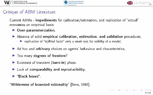
Critique of ABM Literature
Current ABMs - impediments for calibration/estimation, and replication of �actual�economies on empirical basis:
I Over-parameterization,
I Absence of solid empirical calibration, estimation, and validation procedures,I replication of �stylized facts� only a weak test for validity of a model,
I Ad hoc and arbitrary choices on agents' behaviour and characteristics,
I Too many degrees of freedom?
I Existence of transient (burn-in) phase.
I Lack of comparability and reproducibility,
I �Black boxes� .
�Wilderness of bounded rationality� [Sims, 1980].
7 / 43

INSTITUTE FOR ECOLOGICAL ECONOMICS
Economic forecasting: ABM for a small open economyAn empirical ABM that depicts the national economy of Austria.
I Incorporates all economic activities (producing and distributive transactions) asclassi�ed by the European system of accounts (ESA).
I Includes all economic entities: all juridical and natural persons are represented byagents.
I Integrates data from input-output tables (IOTs), national annual sector accounts(NASA), government statistics, census and business demography data, andbusiness surveys.
I Behavioural equations used are standard in literature, e.g.[Delli Gatti et al., 2011, Assenza et al., 2015]
I Parameters are estimated rather than calibrated, no free parameters,I → No �burn-in� phase.
I Empirical validation: compare out-of-sample prediction performance of the ABMwith that of autoregressive (AR), vector autoregressive (VAR) and DSGE modelsestimated on the same observable time series.
8 / 43
INSTITUTE FOR ECOLOGICAL ECONOMICS
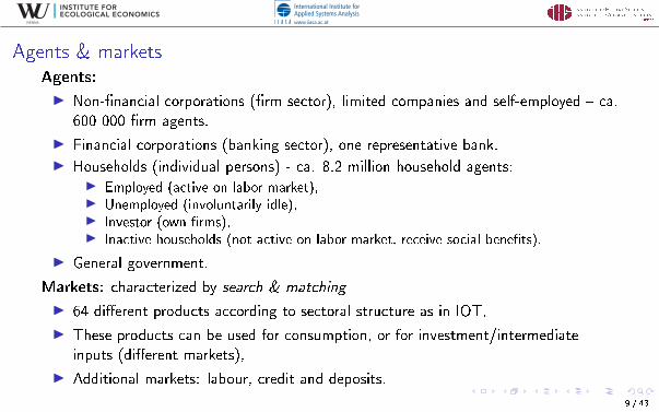
Agents & marketsAgents:
I Non-�nancial corporations (�rm sector), limited companies and self-employed � ca.600 000 �rm agents.
I Financial corporations (banking sector), one representative bank.
I Households (individual persons) - ca. 8.2 million household agents:I Employed (active on labor market),I Unemployed (involuntarily idle),I Investor (own �rms),I Inactive households (not active on labor market, receive social bene�ts).
I General government.
Markets: characterized by search & matching
I 64 di�erent products according to sectoral structure as in IOT,
I These products can be used for consumption, or for investment/intermediateinputs (di�erent markets),
I Additional markets: labour, credit and deposits.
9 / 43

INSTITUTE FOR ECOLOGICAL ECONOMICS
Major Economic Agents and their Interactions
Bonds
Social benefits
Advances
Reserves
TaxesTaxes
Loans
Deposits
Deposits
Taxes
Imports
Imports
Exports
Consumption
Dividends Wages,Dividends
Subsidies,Consumption
10 / 43
INSTITUTE FOR ECOLOGICAL ECONOMICS
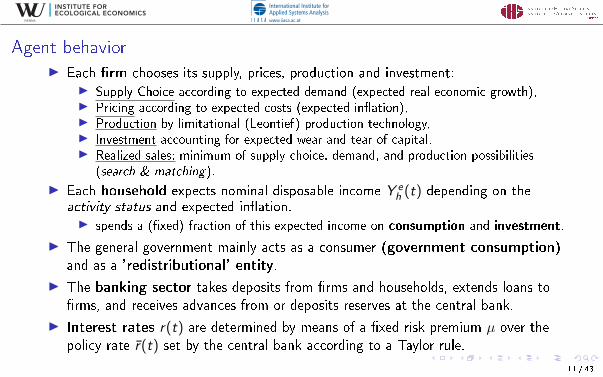
Agent behaviorI Each �rm chooses its supply, prices, production and investment:
I Supply Choice according to expected demand (expected real economic growth),I Pricing according to expected costs (expected in�ation),I Production by limitational (Leontief) production technology,I Investment accounting for expected wear and tear of capital.I Realized sales: minimum of supply choice, demand, and production possibilities
(search & matching).
I Each household expects nominal disposable income Y eh (t) depending on the
activity status and expected in�ation.I spends a (�xed) fraction of this expected income on consumption and investment.
I The general government mainly acts as a consumer (government consumption)and as a 'redistributional' entity.
I The banking sector takes deposits from �rms and households, extends loans to�rms, and receives advances from or deposits reserves at the central bank.
I Interest rates r(t) are determined by means of a �xed risk premium µ over thepolicy rate r̄(t) set by the central bank according to a Taylor rule.
11 / 43

INSTITUTE FOR ECOLOGICAL ECONOMICS
Expectations � parameter-free adaptive learningParameter-free adaptive learning: Agents (�rms and households) act aseconometricians who estimate the parameters of their model to make forecasts of keymacroeconomic aggregates.
Expectations: formed according to an autoregressive model of lag order one (AR(1)).
AR models: Dependent variable x(t) explained by its lag(s) up to order p, and an errorterm ε(t).
The expected real growth rate γe(t) and the expected in�ation rate πe(t) are inferredfrom agents' predictions of (expected) gross domestic product (real GDP, in log levels)and in�ation (the GDP de�ator DEFL, 2010=100), lag order one:
GDPe(t) = αGDPGDP(t − 1) + εGDP(t) (1)
DEFLe(t) = αDEFLDEFL(t − 1) + επ(t) (2)
For both expectation formation and forecasting below, we used the AIC and BICcriterion to determine the optimal lag length for the AR model.
12 / 43

INSTITUTE FOR ECOLOGICAL ECONOMICS
Firms: Supply Choice & Pricing (Adaptive Learning)Supply choice/demand expectations:Firms forms expectations about economic growth (γe(t)) according to AR(1) process,i.e. by parameter-free adaptive learning. Each �rm i adapts desired scale of activity(Qs
i (t)) according to the previous period's demand (Qdi (t − 1)) and the assumptions
about the development of the real growth rate (γe(t))
Qsi (t) = Qe
i (t) = Qdi (t − 1)(1 + γe(t)) (3)
Pricing: according to expected in�ation rate πe(t), cost-structure ('cost-pushin�ation'), unit target operating surplus:
Pi (t) =
Unit labour costs︷ ︸︸ ︷wi (t)(1 + τSIF )P̄HH(t − 1)(1 + πe(t))
αi (t)+
Unit Material costs︷ ︸︸ ︷1
βi
∑g
asg P̄g (t − 1)(1 + πe(t)) +
Unit capital costs︷ ︸︸ ︷δi
κiP̄CF (t − 1)(1 + πe(t))
+ τYi Pi (t − 1)(1 + πe(t))︸ ︷︷ ︸Unit net taxes/subsidies products
+τKiκiω
P̄CF (t − 1)(1 + πe(t))︸ ︷︷ ︸Unit net taxes/subsidies production
+ π̄iPi (t − 1)(1 + πe(t))︸ ︷︷ ︸Target unit operating surplus
(4)
13 / 43

INSTITUTE FOR ECOLOGICAL ECONOMICS
Firms: Output & Investment
Output Yi (t) produced via:(1) intermediate inputs Mi (t), (2) labor Ni (t), (3) capital stock Ki (t − 1),with a �xed coe�cient (Leontief) technology, where the coe�cients are obtained fromIOTs:
αi (t), βi and κi � productivity coe�cients,asg � technologically determined input (�technology�) coe�cients:
(5)Yi (t) = min
(Qs
i (t),βias1
Mi1(t − 1),βias2
Mi2(t − 1), . . . ,βiasg
Mig (t − 1), αi (t)Ni (t), κiKi (t − 1)
)Investment � according to:(1) depreciation rate of capital δi , (2) productivity of capital κi , and (3) desired scale ofactivity Qs
i (t) based on demand expectations,
I di (t) =δiκiQs
i (t) =δiκiQe
i (t) =δiκiQd
i (t − 1)[1 + γe(t)] , (6)
14 / 43
INSTITUTE FOR ECOLOGICAL ECONOMICS
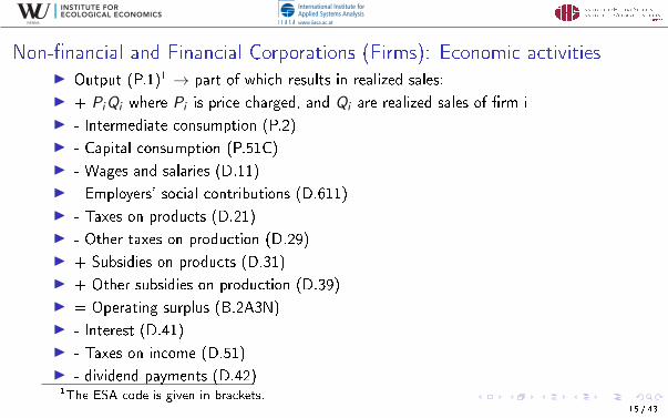
Non-�nancial and Financial Corporations (Firms): Economic activitiesI Output (P.1)1 → part of which results in realized sales:
I + PiQi where Pi is price charged, and Qi are realized sales of �rm i
I - Intermediate consumption (P.2)
I - Capital consumption (P.51C)
I - Wages and salaries (D.11)
I - Employers' social contributions (D.611)
I - Taxes on products (D.21)
I - Other taxes on production (D.29)
I + Subsidies on products (D.31)
I + Other subsidies on production (D.39)
I = Operating surplus (B.2A3N)
I - Interest (D.41)
I - Taxes on income (D.51)
I - dividend payments (D.42)1The ESA code is given in brackets.
15 / 43

Households - income: each household forms expectations on its expected nominal disposableincome Y e
h (t) (i.e. expected net income after taxes and including social or unemployment bene�ts):
Y eh (t) =
(wh(t)
[1− τSIW − τ INC (1− τSIW )
]+ sbother
)P̄HH(t − 1)(1 + πe(t)) if employed(
wh(t) + sbother)P̄HH(t − 1)(1 + πe(t)) if unemployed(
sbinact + sbother)P̄HH(t − 1)(1 + πe(t)) if not economically active
θDIV (1− τ INC )(1− τFIRM) max(0,Πei (t)) + sbother P̄HH(t − 1)(1 + πe(t)) if an investor
θDIV (1− τ INC )(1− τFIRM) max(0,Πek(t)) + sbother P̄HH(t − 1)(1 + πe(t)) if a bank investor
(7)Here,
wh(t) is wage income or unemployment bene�ts (which are a �xed fraction θ of the wage lastearned before the unemployment) of household h,
P̄HH(t − 1) is last period's consumer price index,
Πei (t) are expected pro�ts of �rm i , Πe
k(t) are expected bank pro�ts,
sbinact are social bene�ts for inactive persons (mostly pension payments), sbother social bene�tsdistributed equally to all households
τ INC is the income tax rate, τSIW is the rate of social insurance contributions to be paid by theemployee, θDIV is the dividend payout ratio, and τFIRM the corporate tax rate.

INSTITUTE FOR ECOLOGICAL ECONOMICS
Households: Consumption, Investment & SavingsHouseholds spend a fraction of their expected income on consumption:
Cdh (t) =
ψY eh (t)
1 + τVAT(8)
and on investment:
(9)I dh (t) =ψHY e
h (t)
1 + τCF,
where ψ, ψH are propensities to consume,invest out of expected income; τVAT , τCF arevalue added, investment tax rates. Total household consumption allocated to goods gaccording to �xed coe�cients from IOTs, analogous to �rm investment above.
Households' consumption, investment plans need not be realized (fundamentaluncertainty!): expectation mistakes, search and matching
Savings: di�erence between realized disposable income Yh(t), realized consumptionexpenditure Ch(t), used to accumulate �nancial wealth:
Dh(t) = Dh(t − 1) +
Savings︷ ︸︸ ︷Yh(t)− [(1 + τVAT )Ch(t) + (1 + τCF )Ih(t)] (10)
.17 / 43

INSTITUTE FOR ECOLOGICAL ECONOMICS
Households: Economic activities
I + Wages and salaries (D.11)
I + Property Income (D.4)
I + Mixed Income from Self-Employment (B2A3N)
I + Social bene�ts other than social transfers in kind (D.62)
I + Other current transfers net (D7, D8, D.9)
I - Final consumption expenditure (P.3)
I - Taxes on products (D.21)
I - Taxes on income (D.5)
I - Employees' social contributions (D.612, D.613, D.614)
I - Capital formation (dwellings) (P.51)
18 / 43

INSTITUTE FOR ECOLOGICAL ECONOMICS
General Government: Economic activities
Government mainly acts as a consumer (government consumption) and as a'redistributional' entity: consumes on the goods market to provide a public good,collects taxes, provides transfers.
I + Taxes on income (D.5, D.91)
I + Taxes on products and production (D.2)
I + Property Income (D.4)
I + Social contributions (D.61)
I - Final consumption (P.3)
I - Subsidies (D.3)
I - Interest payments (D.41)
I - Social bene�ts other than social transfers in kind (D.62)
I - Other current expenditures (D.7, D.8, D.9)
19 / 43

INSTITUTE FOR ECOLOGICAL ECONOMICS
Exports, Imports, Government Consumption
According to the small open economy (SoE) assumption as appropriate for theAustrian economy and exogenous policy decisions, these economic aggregates are eitherassumed to be
I exogenously given from data (conditional forecasts),
I or to follow autoregressive (AR) processes according to the SoE setting for Austria
Thus, imports Y I (t), exports CE (t) and government consumption CG (t) (all real andin log levels) either follow AR(1) processes (unconditional forecasting setup):
Y I (t) = αIY I (t − 1) + εI (11)
CE (t) = αECE (t − 1) + εE (12)
CG (t) = αGCG (t − 1) + εG , (13)
or are given exogenously in the conditional forecasting setup.
20 / 43

INSTITUTE FOR ECOLOGICAL ECONOMICS
Parameter setting: European System of AccountsI Input-output tables (IOTs)I National annual sector accounts (NASA)I Government statisticsI Demographic statistics and census dataI Business surveys
Table: National Accounting Data: EUROSTAT Data Tables Used
GDP and main components - output, expenditure and income (quarterly)Symmetric input-output table at basic prices (product by product)Cross-classi�cation of �xed assets by industry/asset (stocks)Balance sheets for non-�nancial assetsNon-�nancial transactionsBusiness demography by legal formCurrent level of capacity utilization in manufacturing industryGovernment revenue, expenditure and main aggregatesGovernment de�cit/surplus, debt and associated dataGovernment expenditure by functionPopulation by current activity status
21 / 43

Table: Unconditional forecasting performance
GDP growth GDP de�ator growth Household consumption Investment Euribor
AR(1) RMSE-statistic for di�erent forecast horizons1q 0.62 0.37 0.66 1.4 0.052q 0.89 0.36 0.93 2.21 0.14q 1.33 0.34 1.32 3.5 0.168q 1.48 0.37 1.57 4.34 0.2112q 1.31 0.33 2 6.09 0.26ABM Percentage gains (+) or losses (-) relative to AR(1) model1q -1.7 (0.02) 0 (0.96) 0.5 (0.94) 8.9 (0.13) -235.7 (0.00)2q -1.8 (0.30) -1.2 (0.29) 0.5 (0.96) 10.2 (0.20) -90.3 (0.19)4q 0.2 (0.93) 1.1 (0.14) 7.1 (0.62) 9.2 (0.28) -15.9 (0.78)8q 5.9 (0.13) 0.4 (0.78) 21.6 (0.04) 29.8 (0.00) 58 (0.00)12q 4.6 (0.54) -0.3 (0.10) 29.8 (0.00) 39.6 (0.00) 79.6 (0.00)DSGE Percentage gains (+) or losses (-) relative to AR(1) model1q -5.7 (0.62) 5.3 (0.59) 7.9 (0.31) 22.1 (0.24) -16 (0.06)2q -3.4 (0.80) -20 (0.17) 7.2 (0.43) 31.4 (0.28) -39.1 (0.01)4q 15.1 (0.17) -8.2 (0.00) 25.3 (0.13) 37.9 (0.26) -70.2 (0.00)8q 39 (0.08) 1.7 (0.43) 10.9 (0.32) 36.1 (0.16) -132.2 (0.00)12q 28.5 (0.00) -4.3 (0.63) 7.1 (0.37) 50.8 (0.00) -139.2 (0.00)
Table: RMSE-statistic for di�erent forecast horizons from 2010:Q2-2016:Q4 of ABM in comparison to AR(1)and DSGE models (unconditional forecasts). Values in brackets indicate p-values of the[Diebold and Mariano, 1995] test on predictive accuracy.

Table: Conditional forecasting (exogenous predictors)GDP growth GDP de�ator growth Household consumption Investment
ARX(1) RMSE-statistic for di�erent forecast horizons1q 0.34 0.38 0.58 1.112q 0.37 0.34 0.75 1.494q 0.41 0.35 0.96 1.258q 0.53 0.35 1.22 1.0712q 0.58 0.41 1.43 1.35�ABMX� (cond. fc.) Percentage gains (+) or losses (-) relative to ARX(1) model1q 3.3 (0.12) -0.9 (0.21) -22.1 (0.19) -1.8 (0.94)2q -0.9 (0.90) -1.1 (0.34) -8.4 (0.62) -11.8 (0.74)4q -23.1 (0.51) 0.8 (0.51) -12.8 (0.55) -107.1 (0.10)8q -1 (0.94) -1 (0.00) 18.8 (0.05) -142.3 (0.03)12q 18.5 (0.00) -1.6 (0.00) 6.6 (0.33) -120.5 (0.06)�DSGEX� (cond. fc.) Percentage gains (+) or losses (-) relative to ARX(1) model1q -60.7 (0.05) 1.4 (0.91) -200.3 (0.08) -1.1 (0.96)2q -105.8 (0.00) -17.1 (0.28) -196.7 (0.09) -3.5 (0.90)4q -105.4 (0.00) -12.4 (0.59) -242.2 (0.12) -86.2 (0.00)8q -144.4 (0.12) -7.7 (0.56) -287.6 (0.00) -117.5 (0.00)12q -160.2 (0.00) -33.9 (0.00) -354 (0.00) -71.9 (0.00)
Table: RMSE-statistic for di�erent forecast horizons from 2010:Q2-2016:Q4 of ABM with 6 predictors incomparison to ARX(1) with the same predictors, as well as to a DSGE model with conditional forecasts.Values in brackets indicate p-values of the [Diebold and Mariano, 1995] test on predictive accuracy.

INSTITUTE FOR ECOLOGICAL ECONOMICS
Out-of-sample Prediction Performance, Growth: 2010:Q4 - 2013:Q4
2010 2011 2012 2013-1
0
1
2
3
4GDP growth (annual)
DATAAR(1)DSGEABM
2010 2011 2012 2013
1
1.5
2
2.5
3
3.5
4Inflation (annual)
2010 2011 2012 2013-1
-0.5
0
0.5
1
1.5
2GDP growth (quarterly)
2010 2011 2012 2013
0
0.5
1
1.5Inflation (quarterly)
Figure: ABM (black), AR(1) (blue), DSGE (red), Eurostat data (dashed); horizon 12q
24 / 43

INSTITUTE FOR ECOLOGICAL ECONOMICS
Out-of-sample Prediction Performance, Quarterly levels: 2010:Q4 - 2013:Q4
2010 2011 2012 20137.4
7.5
7.6
7.7
7.8
7.9
81010 GDP (quarterly)
DATAAR(1)DSGEABM
2010 2011 2012 20133.9
4
4.1
4.2
4.31010Consumption (quarterly)
2010 2011 2012 20131.6
1.65
1.7
1.75
1.8
1.85
1.91010 Investment (quarterly)
2010 2011 2012 2013
1.51
1.515
1.52
1.525
1.53
1.535
1.54106 Government (quarterly)
2010 2011 2012 20133.85
3.9
3.95
4
4.05
4.1
4.15106 Exports (quarterly)
2010 2011 2012 20133.6
3.65
3.7
3.75
3.8
3.85
3.9106 Imports (quarterly)
Figure: ABM (black), AR(1) (blue), DSGE (red), Eurostat data (dashed); horizon 12q 25 / 43

INSTITUTE FOR ECOLOGICAL ECONOMICS
National accountingProduction approach
2010 2011 2012 20130
0.5
1
1.5
2
2.5
3
3.510
11
A
B, C, D and E
F
G, H and I
J
K
L
M and N
O, P and Q
R and S
Taxes less subsidies
Income approach
2010 2011 2012 20130
0.5
1
1.5
2
2.5
3
3.510
11
Wages
Social contributions
Gross operating surplus
Taxes less subsidies on production
Taxes less subsidies on products
Expenditure approach
2010 2011 2012 20130
0.5
1
1.5
2
2.5
3
3.510
11
Household consumption
Government consumption
Capital formation
Net exports
Figure: GDP: production, income, and expenditure approaches, ABM (solid) vs. data (dashed)26 / 43

Figure: Sectoral decomposition: ABM simulations (solid), observed data (dashed)
2010 2011 2012 2013
2000
2200
2400
2600A01
2010 2011 2012 2013
1050
1100
1150
1200
A02
2010 2011 2012 2013
14
16
18
20
22
A03
2010 2011 2012 2013
800
1000
1200B
2010 2011 2012 2013
4600
4800
5000
C10-C12
2010 2011 2012 2013
900
1000
1100C13-C15
2010 2011 2012 2013
1600
1700
1800C16
2010 2011 2012 2013
1600
1650
1700
C17
2010 2011 2012 2013
800
900
1000
C18
2010 2011 2012 2013
0
100
200
C19
2010 2011 2012 2013
1000
1200
1400
C20
2010 2011 2012 2013
1200
1250
1300
1350C21
2010 2011 2012 2013
1700
1800
1900
C22
2010 2011 2012 2013
1900
2000
2100
2200C23
2010 2011 2012 2013
2900
3000
3100
3200C24
2010 2011 2012 2013
3800
4000
4200
4400C25
2010 2011 2012 2013
1800
2000
2200C26
2010 2011 2012 2013
3000
3200
3400
3600
C27
2010 2011 2012 2013
4500
5000
5500
6000C28
2010 2011 2012 2013
2400
2600
2800
3000
C29
2010 2011 2012 2013
800
900
1000
C30
2010 2011 2012 2013
2100
2200
2300
C31_C32
2010 2011 2012 2013
3000
3200
3400C33
2010 2011 2012 2013
4400
4600
4800
5000
5200
D
2010 2011 2012 2013
400
500
600E36
2010 2011 2012 2013
2600
2700
2800
2900E37-E39
2010 2011 2012 2013
1.7
1.75
1.8
1.85
104 F
2010 2011 2012 2013
3600
3800
4000G45
2010 2011 2012 2013
1.8
1.9
210
4 G46
2010 2011 2012 2013
1.25
1.3
1.35
1.410
4 G47
2010 2011 2012 2013
6500
7000
7500
8000H49
2010 2011 2012 2013
18
20
22
24H50
2010 2011 2012 2013
400
500
600
H51
2010 2011 2012 2013
5000
5200
5400
5600H52
2010 2011 2012 2013
1250
1300
1350
1400H53
2010 2011 2012 2013
1.3
1.4
1.510
4 I
2010 2011 2012 2013
1150
1200
1250
1300J58
2010 2011 2012 2013
800
900
1000
J59_J60
2010 2011 2012 2013
2400
2600
2800
3000J61
2010 2011 2012 2013
5000
6000
7000
J62_J63
2010 2011 2012 2013
7500
8000
8500
9000K64
2010 2011 2012 2013
2200
2400
2600
K65
2010 2011 2012 2013
900
1000
1100
1200K66
2010 2011 2012 2013
2.6
2.8
310
4 L
2010 2011 2012 2013
7500
8000
8500
M69_M70
2010 2011 2012 2013
4000
4500
5000M71
2010 2011 2012 2013
6000
7000
8000M72
2010 2011 2012 2013
1400
1600
1800M73
2010 2011 2012 2013
1000
1100
1200M74_M75
2010 2011 2012 2013
5000
5200
5400
5600N77
2010 2011 2012 2013
3800
4000
4200
N78
2010 2011 2012 2013
400
450
500
550N79
2010 2011 2012 2013
4000
4200
4400
4600
N80-N82
2010 2011 2012 2013
1.35
1.4
1.45
1.510
4 O
2010 2011 2012 2013
1.3
1.35
1.4
1.4510
4 P
2010 2011 2012 2013
1.3
1.35
1.4
1.4510
4 Q86
2010 2011 2012 2013
4000
4200
4400
4600
Q87_Q88
2010 2011 2012 2013
2200
2300
2400
R90-R92
2010 2011 2012 2013
1050
1100
1150
1200R93
2010 2011 2012 2013
1700
1800
1900
2000S94
2010 2011 2012 2013
550
600
650
S95
2010 2011 2012 2013
2000
2100
2200
S96
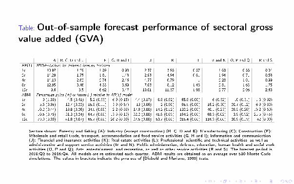
Table: Out-of-sample forecast performance of sectoral grossvalue added (GVA)
A B, C, D and E F G, H and I J K L M and N O, P and Q R and S
AR(1) RMSE-statistic for di�erent forecast horizons
1q 10.97 1.29 1.39 0.98 2.37 3.95 0.37 1.68 0.55 0.342q 14.29 1.75 1.81 1.48 2.93 4.94 0.61 1.94 0.71 0.584q 14.13 2.62 2.74 2.46 4.77 6.79 1 2.28 1.01 0.998q 12.95 3.46 4.33 3.69 7.03 8.12 1.45 2.81 1.63 1.7512q 9.6 3.5 6.62 3.47 10.01 11.57 1.98 2.77 2.06 2.63ABM Percentage gains (+) or losses (-) relative to AR(1) model
1q 0 (1.00) 4.5 (0.41) 5.2 (0.55) -6.9 (0.15) 4.4 (0.17) 0.8 (0.92) -65.8 (0.00) -6 (0.52) 10 (0.31) -1.5 (0.92)2q -5.6 (0.65) 12.7 (0.22) 15.8 (0.11) -3.9 (0.67) 13 (0.06) 2 (0.90) -95.5 (0.00) -16.2 (0.30) 20.7 (0.12) 6.9 (0.83)4q -10.2 (0.44) 19.8 (0.26) 34.5 (0.00) 2.2 (0.88) 17.9 (0.00) 14.2 (0.52) -132.2 (0.00) -40.1 (0.23) 29.8 (0.20) 19.2 (0.60)8q -10.5 (0.76) 31.3 (0.24) 64.7 (0.00) 13.9 (0.13) 32.2 (0.00) 41.9 (0.09) -194.2 (0.00) -68.3 (0.02) 3.9 (0.92) 25.5 (0.45)12q -79.3 (0.00) 41.8 (0.07) 65.7 (0.00) 26.2 (0.00) 37.5 (0.00) 53.7 (0.00) -215.4 (0.00) -116.3 (0.00) -20.9 (0.59) 42 (0.00)
Sectors shown: Forestry and �shing (A); Industry (except construction) (B, C, D and E); Manufacturing (C); Construction (F);Wholesale and retail trade, transport, accommodation and food service activities (G, H and I); Information and communication(J); Financial and insurance activities (K); Real estate activities (L); Professional, scienti�c and technical activities, as well asadministrative and support service activities (M and N); Public administration, defence, education, human health and social workactivities (O, P and Q); Arts, entertainment, and recreation, as well as other service activities (R and S). The forecast period is2010:Q2 to 2016:Q4. All models are re-estimated each quarter. ABM results are obtained as an average over 500 Monte Carlosimulations. The values in brackets indicate the p-values of [Diebold and Mariano, 1995] tests.

INSTITUTE FOR ECOLOGICAL ECONOMICS
Conclusions and Contributions to the Literature
Q1: How can ABMs be empirically estimated in a solid way?
Answer: Development of a large-scale empirical ABM that is estimated rather thancalibrated, avoids burn-in phase → �rst ABM comprehensively estimated to anational economy (Austria).
Q2: How can ABMs be empirically validated comprehensively, and how can they bemade comparable to standard methods of economic analysis?
Answer: This ABM is able to compete with vector autoregressive (VAR),autoregressive (AR) and DSGE models in out-of-sample prediction.
Q3: Is it possible to make ABMs usable for economic forecasts and simulationexperiments for �actual� economies (economic and other shocks, policy changes, etc.)?
Answer: Applications � economic forecasting and indirect economic e�ects from
natural disasters for the Austrian national economy.
29 / 43

INSTITUTE FOR ECOLOGICAL ECONOMICS
Outlook and future research�Renewal� of structural macro-econometric Keynesian models? Confront the Lucascritique from new angle:I Construct large-scale empirical models that include expectation formation and
learning mechanisms (adaptive but also forward-looking behaviour),I Include sophisticated endogenous model dynamics (emergence) + highly detailed
micro-foundations.
'Simulation Laboratory' for economic analysis:I Prediction of economic trends (growth, in�ation, structural change, ...) on a
sectoral level. Quantify e�ects of policy changes for single households/�rms.
Possibilities for extension (among many others):
1. So far: Integration of �big data 1.0�. Potential next steps: more detailedmicro-data, e.g.: SABINA database (�rms); household surveys (EU-SILC orHFCS), or full population coverage data: Austrian social security data.
2. More detailed �nancial market (linked to the real economy, endogenous �nancialcycles); up-scale model to euro area.
3. More sophisticated expectation formation mechanisms, e.g. VARexpectations, or more forward looking expectation mechanisms. 30 / 43

INSTITUTE FOR ECOLOGICAL ECONOMICS
Appendix
Thank you for your attention!
Further details on the agent-based model areincluded below.
31 / 43

INSTITUTE FOR ECOLOGICAL ECONOMICS
LimitationsThe following limitations apply for our work:
I Model takes a short- to medium term perspective due omission of some drivers oflong-term economic growth:
I no demographic change (population growth)I no productivity growth of labor due to increased skills and competences (education)I no e�ect on government �nancing conditions (e.g. interest rates) due to increased
government debt and de�cit levels
I some structural features of labor market not incorporated:
I no skill mismatches and other structurally determined labor market frictionsI no migration from workers active on labor market (employed and unemployed) to inactive
persons and vice versa (no depiction of 'hidden labor force')
I no structural di�erences between �rms producing for domestic market and exporting
�rms (though empirical evidence suggests the contrary)
I no correlation assumed between structural features of �rms (e.g. size) andtechnological parameters derived from IOTs (e.g. no economies of scale)
These issues will be addressed in the ongoing further development of the model!32 / 43

INSTITUTE FOR ECOLOGICAL ECONOMICS
IO Sectors - NACE Rev. 2 Classi�cationStatistical classi�cation of economic activities in the European Community
33 / 43
INSTITUTE FOR ECOLOGICAL ECONOMICS
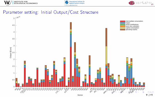
Parameter setting: Initial Output/Cost Structure
A01A02A03 B
C10-C
12
C13-C
15C16C17C18C19C20C21C22C23C24C25C26C27C28C29C30
C31_C
32C33 DE36
E37-E
39 FG45G46G47H49H50H51H52H53
IJ5
8
J59_
J60J6
1
J62_
J63K64K65K66 L
M69
_M70
M71
M72
M73
M74
_M75N77N78N79
N80-N
82 O PQ86
Q87_Q
88
R90-R
92R93S94S95S96
Sector
0
0.5
1
1.5
2
2.5
3
3.5
4
4.5
5
Out
put [
Eur
o]
×1010
intermediate consumptionwagessocial contributionstaxes less subsidiescapital consumptionoperating surplus
Figure: Distribution of output and cost structure by sector used as initial values for modelsimulations from observed data of Austria
34 / 43

INSTITUTE FOR ECOLOGICAL ECONOMICS
Parameter setting: Initial number of �rms/employees
A01A02A03 B
C10-C
12
C13-C
15C16C17C18C19C20C21C22C23C24C25C26C27C28C29C30
C31_C
32C33 DE36
E37-E
39 FG45G46G47H49H50H51H52H53
IJ5
8
J59_
J60J6
1
J62_
J63K64K65K66 L
M69
_M70M
71M
72M
73
M74
_M75N77N78N79
N80-N
82 O PQ86
Q87_Q
88
R90-R
92R93S94S95S96
Sector
0
1
2
3
4
5
6
7
8
9
10
Num
ber
firm
s
×104
0
0.5
1
1.5
2
2.5
3
3.5
4
Num
ber
empl
oyee
s
×105
firmsemployees
Figure: Distribution of number of �rms and employees by sector used as initial values for modelsimulations from observed data of Austria
35 / 43
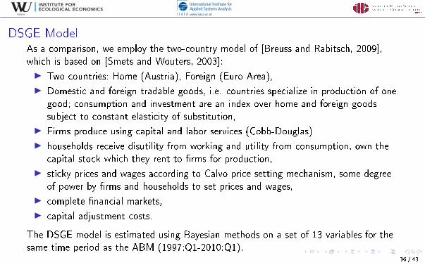
INSTITUTE FOR ECOLOGICAL ECONOMICS
DSGE ModelAs a comparison, we employ the two-country model of [Breuss and Rabitsch, 2009],which is based on [Smets and Wouters, 2003]:
I Two countries: Home (Austria), Foreign (Euro Area),
I Domestic and foreign tradable goods, i.e. countries specialize in production of onegood; consumption and investment are an index over home and foreign goodssubject to constant elasticity of substitution,
I Firms produce using capital and labor services (Cobb-Douglas)
I households receive disutility from working and utility from consumption, own thecapital stock which they rent to �rms for production,
I sticky prices and wages according to Calvo price setting mechanism, some degreeof power by �rms and households to set prices and wages,
I complete �nancial markets,
I capital adjustment costs.
The DSGE model is estimated using Bayesian methods on a set of 13 variables for thesame time period as the ABM (1997:Q1-2010:Q1).
36 / 43

GDP =
Total sales of goods and services︷ ︸︸ ︷611278∑i=1
(1− τYi )Pi (t)Yi (t) −
Intermediate inputs︷ ︸︸ ︷∑g,s,i∈Is
P̄g (t)asgYi (t)
βi(Production approach)
=
Household consumption︷ ︸︸ ︷8248321∑
h=1
Ch(t) +
Government consumption︷ ︸︸ ︷∑j
Cj(t) +
Gross �xed capital formation︷ ︸︸ ︷8248321∑
h=1
Ih(t) +611278∑i=1
P̄CF (t)Ii (t)
+
Changes in inventories︷ ︸︸ ︷611278∑i=1
Pi (t)∆Si (t) +∑
g,s,i∈Is
P̄g (t)
(∆Mig (t) − asg
Yi (t)
βi
)+
Exports︷ ︸︸ ︷∑l
(Cl(t)
−
Imports︷ ︸︸ ︷∑m
Pm(t)Qm(t))−
Net taxes on products︷ ︸︸ ︷∑i
τYi Pi (t)Yi (t) (Expenditure approach)
= (1 + τSIF )P̄HH(t)8248321∑
h=1
wh(t)︸ ︷︷ ︸Compensation of employees
+611278∑i=1
(Πi (t) + r(t)Li (t) + P̄CF (t)
δiκi
Yi (t)
)︸ ︷︷ ︸
Gross operating surplus and mixed income
+∑i
τKi Pi (t)Yi (t)︸ ︷︷ ︸Net taxes on production
(Income approach)
INSTITUTE FOR ECOLOGICAL ECONOMICS
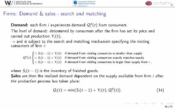
Firms: Demand & sales - search and matching
Demand: each �rm i experiences demand Qdi (t) from consumers.
The level of demand: determined by consumers after the �rm has set its price andcarried out production Yi (t),→ and is subject to the search and matching mechanism specifying the visitingconsumers of �rm i :
Qdi (t)
< Si (t − 1) + Yi (t) if demand from visiting consumers is smaller than supply
= Si (t − 1) + Yi (t) if demand from visiting consumers exactly matches supply
> Si (t − 1) + Yi (t) if demand from visiting consumers is larger than supply from i ,
where Si (t − 1) is the inventory of �nished goods.Sales are then the realized demand dependent on the supply available from �rm i afterthe production process has taken place:
(14)Qi (t) = min(Si (t − 1) + Yi (t),Qdi (t)) .
38 / 43

INSTITUTE FOR ECOLOGICAL ECONOMICS
General Government: Revenues Y G (t)
(15)
Y G (t) =
Social security contributions︷ ︸︸ ︷(τSIF + τSIW )P̄HH(t)
∑h∈HE (t)
wh(t) +
Labour income taxes︷ ︸︸ ︷τ INC (1− τSIW )P̄HH(t)
∑h∈HE (t)
wh(t)
+
Value added taxes︷ ︸︸ ︷τVAT
∑h
Ch(t) +
Capital income taxes︷ ︸︸ ︷τ INC (1− τFIRM)θDIV
(∑i
max(0,Πi (t)) + max(0,Πk(t))
)
+
Corporate income taxes︷ ︸︸ ︷τFIRM
(∑i
max(0,Πi (t)) + max(0,Πk(t))
)+ τCF
∑h
Ih(t)︸ ︷︷ ︸Taxes on capital formation
+∑s,i∈Is
τYi Pi (t)Yi (t)
︸ ︷︷ ︸Net taxes/subsidies on products
+ P̄CF (t)∑i
τKi Ki (t)︸ ︷︷ ︸Net taxes/subsidies on production
+ τEXPORT∑l
Cl(t)︸ ︷︷ ︸Export taxes
.
39 / 43

INSTITUTE FOR ECOLOGICAL ECONOMICS
General Government: De�cit & Debt
The government de�cit (or surplus) resulting from its redistributive activities is
(16)
ΠG (t) =
Government revenues︷ ︸︸ ︷Y G (t) −
Government consumption︷ ︸︸ ︷∑j
Cj(t) −
Interest payments︷ ︸︸ ︷rGLG (t)
−∑
h∈H inact
P̄HH(t)sbinact +∑
h∈HU (t)
P̄HH(t)wh(t) +∑h
P̄HH(t)sbother
︸ ︷︷ ︸Social bene�ts and transfers
The government debt is determined by the year-to-year de�cits/surpluses of thegovernment sector:
(17)LG (t) = LG (t − 1) + ΠG (t)
40 / 43

INSTITUTE FOR ECOLOGICAL ECONOMICS
The Banking Sector
The bank takes deposits from �rms and households, and extends a total amount ofloans Ltot(t) =
∑Ii=1 Li (t)
The bank will grant a loan to �rm i up to the point where the borrower's leverage (orloan-to-value) ratio after the loan,
(18)Li (t)
P̄CF (t)Ki (t)≤ ζLTV
is below ζLTV , which is a constant.
Furthermore, the bank is subject to minimum capital requirements, i.e. it can onlyextend total loans up to a maximum multiple of its equity base or net worth EB(t).
The interest rate r(t) for bank credit to �rms is determined by means of a �xed riskpremium µ over the policy rate r̄(t) set by the central bank according to a Taylor rule:
r(t) = r̄(t) + µ . (19)
41 / 43
INSTITUTE FOR ECOLOGICAL ECONOMICS
References I
Assenza, T., Delli Gatti, D., and Grazzini, J. (2015).Emergent dynamics of a macroeconomic agent based model with capital andcredit.Journal of Economic Dynamics and Control, 50:5�28.
Breuss, F. and Rabitsch, K. (2009).An estimated two-country dsge model auf austria and the euro area.Empirica, 36:123�158.
Delli Gatti, D., Desiderio, S., Ga�eo, E., Cirillo, P., and Gallegati, M. (2011).Macroeconomics from the Bottom-up.Springer Milan.
Diebold, F. X. and Mariano, R. S. (1995).Comparing predictive accuracy.Journal of Business & Economic Statistics, 13(3).
42 / 43

INSTITUTE FOR ECOLOGICAL ECONOMICS
References II
Poledna, S., Miess, M., and Hommes, C. (2019).Economic forecasting with an agent-based model.SSRN Working Paper.https://papers.ssrn.com/sol3/papers.cfm?abstract_id=3484768.
Sims, C. (1980).Macroeconomics and reality.Econometrica, Vol. 48, No. 1:1�48.
Smets, F. and Wouters, R. (2003).An estimated dynamic stochastic general equilibium model of the euro area.Journal of the European Economic Association, 1(5):1123�1175.
43 / 43