economic fundamentals in local housing …urbanpolicy.berkeley.edu/pdf/hq_jors06.pdf · changes in...

JOURNAL OF REGIONAL SCIENCE, VOL. 46, NO. 3, 2006, pp. 425–453

ECONOMIC FUNDAMENTALS IN LOCAL HOUSINGMARKETS: EVIDENCE FROM U.S. METROPOLITAN REGIONS

Min HwangDepartment of Real Estate, School of Design and Environment, National Universityof Singapore, 4 Architecture Drive, Singapore 117566. E-mail: [email protected]

John M. QuigleyDepartment of Economics, 549 Evans Hall, University of California, Berkeley,CA 94720-3880. E-mail: [email protected]

ABSTRACT. This paper investigates the effects of national and regional economic con-ditions on outcomes in the single-family housing market: housing prices, vacancies, andresidential construction activity. Our three-equation model confirms the importance ofchanges in regional economic conditions, income, and employment on local housing mar-kets. The results also provide the first detailed evidence on the importance of vacanciesin the owner-occupied housing market on housing prices and supplier activities. The re-sults also document the importance of variations in materials, labor and capital costs,and regulation in affecting new supply. Simulation exercises, using standard impulseresponse models, document the lags in market responses to exogenous shocks and thevariations arising from differences in local parameters. The results also suggest the im-portance of local regulation in affecting the pattern of market responses to regional incomeshocks.

1. INTRODUCTION

Housing markets are local, and housing market outcomes reflect localeconomic conditions. Housing prices are bid up as a result of better employ-ment opportunities and higher incomes enjoyed by residents in an expandingmetropolitan market. Changes in the distribution of income are reflected inthe distribution of prices and housing amenities. Similarly, housing vacancyrates can be expected to decline when the local economy improves and as thedemand for housing increases. Finally, residential construction and building ac-tivity are responsive to housing prices, vacancy rates, and the health of the localeconomy. As higher incomes increase the demand for housing, prices are bid up;new construction becomes more profitable, inducing supplier activity. Dwellingsthat would otherwise become vacant remain occupied, and some dwellings thatwould otherwise leave the housing stock are renovated for continued use.

This paper considers the inter-relationship among these three forms ofeconomic behavior in the context of local housing markets. We model the

Received: November 2004; Revised: May 2005; Accepted: July 2005.

C© Blackwell Publishing, Inc. 2006.Blackwell Publishing, Inc., 350 Main Street, Malden, MA 02148, USA and 9600 Garsington Road, Oxford, OX4 2DQ, UK.

425

426 JOURNAL OF REGIONAL SCIENCE, VOL. 46, NO. 3, 2006

FIGURE 1: Course of Real Housing Prices in Nine Metropolitan Areas,1975–2000.

relationship among the prices of owner-occupied housing, vacancy rates, andhousing supplier activity in response to the exogenous factors, which affect thefortunes of the regional economy. We also recognize the importance of local landuse and building regulations in affecting the operation of the owner-occupiedhousing market.

Our analysis uses U. S. metropolitan areas (MSAs) as units of observation,and we follow a panel of 74 MSAs over the 13-year period, 1987–1999. The panelincludes all U.S. metropolitan areas for which annual data are available on theprices of owner−occupied housing, on the vacancy rates in single-family hous-ing, and on supplier activity (i.e., the number of permits issued for constructionof new single-family housing).

Figure 1 illustrates the course of housing prices during 1975–2000 for nineof the MSAs in the sample we analyze below.1 Note the enormous variationin the course of house prices. For the three California housing markets de-picted, real prices more than tripled between 1975 and 1999. For the least

1The figure relies upon the price series maintained by the U.S. Office of Federal HousingEnterprise Oversight, as described in Section V.

C© Blackwell Publishing, Inc. 2006.

HWANG AND QUIGLEY: EVIDENCE FROM U.S. METROPOLITAN REGIONS 427

-10 -5 0 5 10 15 20 25 30-10

-5

0

5

10

15

20

25

30

Percentage Change of Housing Price in Previous Year

Pe

rce

nta

ge

Ch

an

ge

of

Ho

usin

g P

rice

in

Cu

rre

nt Y

ea

r

FIGURE 2: Current Real House Price Changes vs. Lagged House PriceChanges, 1987–1999∗ (74 metropolitan areas).

∗The regression relationship (t-ratios in parentheses) between the percentage change in realhousing prices in the current year, yt, and the percentage change in the previous year, yt −1, is

yt = 0.2948 + 0.4585yt −1

(2.029) (15.02) R2 = 0.234.

volatile markets in the sample (Houston, Albany, and Oklahoma City), nominalhousing prices doubled during the past quarter century. As noted in the figure,real housing prices in these latter markets were stagnant. What causes thisenormous variation?

Figures 2, 3, and 4 illustrate some key relationships explored in this paper.Figure 2 investigates the predictability of housing price changes using our panelof MSAs covering 1987–1999. It presents the current annual real price changesin each of the 74 markets as a function of their lagged values. There is clearlya strong positive relationship, suggesting that lags and slow adjustment tomarket conditions are crucial to understanding the course of prices.

Figure 3 indicates the bivariate relationship between annual changes invacancy rates for single-family dwellings and changes in their prices, while



-4 -3 -2 -1 0 1 2 3-15

-10

-5

0

5

10

15

20

25

Changes in Vacancy Rates

Perc

enta

ge C

hange in H

ousin

g P

rice

FIGURE 3: Changes in Real House Prices vs. Changes in Vacancy Rates,1987–1999∗ (74 metropolitan areas).

∗The regression relationship (t-ratios in parentheses) between the percentage change in realhousing prices, yt, and changes in vacancy rate, xt, is

yt = 0.3029 – 0.2975xt

(1.827) (1.314) R2 = 0.0023.

Figure 4 illustrates the relationship between annual changes in house pricesand the number of building permits issued for new construction of single-familyhousing in these same metropolitan areas.2 These two figures provide littleevidence of the systematic relationships postulated by economic theory. In par-ticular, there is very weak evidence in the simple diagram that housing pricesdecrease as vacancy rates increase. There is some evidence that increases insupplier activity, measured by building permits, affect housing prices. But therelationship is very weak. Is there any strong empirical link between vacancies,new supply, and housing prices?

In this paper, we develop a model relating exogenous changes in regionalemployment and incomes, construction costs and macro economic conditions

2As noted below, data for both vacancy rates and building permits are maintained by the USCensus Bureau.



0 5 10 15-15

-10

-5

0

5

10

15

20

25P

erc

en

tag

e C

ha

ng

e in

Ho

usin

g P

rice

Building Permits as Percentage of Number of Households

FIGURE 4: Changes in Real House Prices vs. Building Permits1987–1999∗ (74 metropolitan areas).

∗The regression relationship (t-ratios in parentheses) between the percentage change in realhousing prices, yt, and building permit, xt, is

yt = 0.1249 + 0.0978xt

(0.677) (2.188) R2 = 0.0064.

to these measures of the health of housing markets—prices, vacancies, andnew construction. The model is estimated in several variants, and we simulatethe responsiveness of the housing market to local economic conditions. Themodel indicates the strong interdependency between the state of the macroeconomy, the state of the regional economy, and outcomes in the housing market.The results also suggest the key role of local regulation in affecting housingoutcomes.

In Section 2 below, we relate our work to previous attempts to developregional models of the housing market. Section 3 presents an overview of thedata and the methodology we use, as well as the relationships among the variousmeasures of the housing market. Section 4 presents data. Section 5 presentsour statistical results and the simulations based upon them. Section 6 is a briefconclusion.



2. ANTECEDENTS

A simple model of supply and demand at the regional level motivates thechoice of variables to explain outcomes in the housing market over time. Hous-ing demand is a function of prices and incomes and perhaps demographic vari-ables as well. Housing supply is a function of profitability, which depends uponhousing prices and input prices, including the costs of labor, materials, financ-ing, and regulations inhibiting new construction. Vacancy rates in existinghousing reflect the difference between aggregate supply and demand in themarket in any period.

Several early papers (following Reid, 1962; Muth, 1960, 1968) analyzedvariations in housing prices across metropolitan areas, focusing on the re-duced form of relationship between the prices of owner-occupied housing andmetropolitan characteristics. Using these models, it is easy to describe the de-velopment of house prices, but it is quite difficult to make inferences aboutstructural parameters or about causation.3

In contrast, a few more recent studies have investigated structural relation-ships among housing market outcomes. Poterba (1984) analyzed the interactionbetween movements in prices and housing stocks, modeled as a two-equationsystem. The growth of housing prices is represented as a function of the dif-ference between current prices and imputed rentals, while the growth of thehousing stock is related to real housing prices (as a proxy for profitability) andto the size of the current stock. In this simple stock-flow model, there are noleads or lags. Vacancies in the housing stock are ignored.

DiPasquale and Wheaton (1994) specified a model for housing demand inwhich the price of owner-occupied housing within a given housing market is afunction of the current stock of single-family housing relative to the numberof households, their age-expected homeownership rate,4 the cost of renting rel-ative to owning in the market, and the average household income within themarket. In a second equation, the authors modeled housing starts as a functionof current prices, costs, and the stock of housing, as well as employment andtime on the market for new units. Most of supplier behavior in this model isexplained by exogenous changes in interest rates, employment levels, and timeon the market. The authors interpret this latter variable as evidence of slowadjustment in housing markets.

Follain and Velz (1995) developed a structural model of housing markets atthe metropolitan level, in part to reflect the importance of turnover (the inverseof time on the market) in housing markets. Their structural model consistsof four equations predicting the turnover rate, housing size, housing prices,and household formation, respectively. Follain and Velz found that housing

3Tests of the efficient functioning of housing markets based on these reduced form modelsare in fact joint tests of the efficiency of the housing market together with the underlying structuralmodels used to derive reduced form relationships (Follain and Velz, 1995).

4The age-expected homeownership rate is a simple transformation of the age distribution ofadults in the housing market.



prices and turnover are negatively related; they attribute this to the reducedimportance of down payment constraints since the mid 1980s. However, theirestimates of some key structural parameters are quite large indeed (e.g., theestimated price elasticity of housing supply is about six).

In assessing this previous work on the determinants of housing price vari-ations, several factors are worth noting. First, none of these empirical modelsconsiders that trends in house prices or new construction might be mitigatedby changes in vacancy rates for owner-occupied housing. This is in contrast toextensive empirical analyses of the rental market (e.g., Rosen and Smith, 1983;Igarashi, 1992; Read, 1993; Hendershott et al., 2000; Gabriel and Nothaft, 1988,2001), which emphasize the inverse relationship between rents and vacancyrates across markets. Second, equations explaining variations in housing sup-ply are often unsatisfactory, in contrast to demand equations, which tend to fitthe data reasonably well. The estimated supply elasticity often has a negativesign, an insignificant effect, or an implausibly large magnitude. Third, with oneexception, these systems of structural equations applied to housing markets aretested on aggregate national time-series data despite the local nature of hous-ing markets. This limitation no doubt reflects difficulties of data assembly atthe metropolitan level.

3. OVERVIEW OF THE MODEL

Our model of regional housing markets is based upon a panel of U.S.metropolitan areas, including all markets for which annual data on housingprices, vacancies, and construction activity are available for owner-occupiedhousing. Of the 334 metropolitan housing markets (MSAs) in the United States,consistent measures of house prices are available for 120, beginning in 1975.Annual measures of the stock of owner-occupied housing, vacancy rates, andsupplier activity (i.e., building permits) are available for only 75 MSAs and onlyfor the period 1987–1999. Our analysis is based upon 962 observations report-ing a panel of 74 MSAs observed annually during the period 1987–1999.5

Some of the key bivariate relationships in this panel of housing marketsare reported in the Section I. Figures 5, 6, and 7 present additional descrip-tive information. Figure 5 suggests that there is a strong positive relationshipbetween price appreciation in these markets and a measure of the restrictive-ness of regulations covering new construction.6 Figure 6 reports a positive, butrather weak, relationship between price appreciation and income growth, whileFigure 7 reports the absence of any simple relationship between house price ap-preciation and employment growth. These puzzles and suggestive relationshipsmotivate our systematic research.

5For one MSA (Scranton, PA) house prices are not available, but vacancy rates, supplieractivity, and housing stock measures are.

6Glaeser et al. (2003) attribute substantial difference between prices and production costs ofManhattan condominiums to land-use regulations. See Quigley and Rosenthal (2005) for a reviewof empirical evidence.



16 18 20 22 24 26 28 30

-1

0

1

2

3

4

5

Regulation Index

Ave

rage P

erc

enta

ge C

hange in H

ousin

g P

rice

FIGURE 5: Average Real House Price Appreciation vs. Regulation Index∗

(74 metropolitan areas).∗The regression relationship (t-ratios in parentheses) between the percentage change in average

real housing prices, yt, and the regulation index, xt, is

yt = −0.0092 + 0.0006xt

(0.799) (5.688) R2 = 0.310.

Our empirical model consists of three equations describing the movementof housing prices, housing supply, and vacancies in the market for owner-occupied housing. In this section, we describe the key features of the model,deferring issues related to data, measurement, and estimation technique toSection IV.

Housing Prices

Our analysis of housing prices is based upon an extension of the work ofDiPasquale and Wheaton (1994), which considers the distinction between thenumber of households in the housing market and their individual demands forowner occupancy. We extend the model to include vacancies

Ht · Dt = OCt = St − Vt = St−1 + Nt − Vt(1)



4.8 5 5.2 5.4 5.6 5.8 6 6.2 6.4 6.6-1

0

1

2

3

4

5

Percentage Change in Income

Perc

enta

ge C

hange in H

ousin

g P

rice

FIGURE 6: Average Real House Price Appreciation vs. Income Growth∗

(74 metropolitan areas).∗The regression relationship (t-ratios in parentheses) between the percentage change in average

real housing prices, yt, and the percentage change in real income, xt, is

yt = −1.2393 + 0.4461xt

(0.584) (1.207) R2 = 0.020.

where Ht is the total number of households in a metropolitan market at the timet, Dt is the proportionate demand for owner occupancy, OCt is the number ofoccupied units of owner housing, St is the total stock of owner-occupied housing,Vt is the number of vacancies, and Nt is the number of newly constructed owner-occupied units.7 The subscript i distinguishing metropolitan area is suppressed

7Our model concentrates on owner-occupied housing, considering rental housing only to theextent that relative prices by tenure type affect tenure choice and to the extent that the level of div-idends (rents) affects asset prices (house values). Thus we assume that the stock of owner-occupiedhousing, St, may decline through depreciation but not through conversion to rental units. Of course,this is not literally true, but structural characteristics do inhibit conversions in tenure type. For ex-ample, as estimated in the 2001 American Housing Survey, 88 percent of single detached structuresare owner-occupied, and 88 percent of apartment dwellings are renter-occupied. A more completemodel would allow for the rental of single detached housing and the conversion of apartments tocondominiums. But this would be a much more complicated model.



0 1 2 3 4 5 6-1

0

1

2

3

4

5

Percentage Change in Employment

Pe

rce

nta

ge

Ch

an

ge

in

Ho

usin

g P

rice

FIGURE 7: Average Real House Price Appreciation vs. Employment Growth∗∗The regression relationship (t-ratios in parentheses) between the percentage change in average

real housing prices, yt, and the percentage change in employment, xt, is

yt = 5.7309 – 0.0206xt

(4.586) (0.188) R2 = 0.0005.

for ease of presentation. Following DiPasquale and Wheaton (1994), individualdemand for owner-occupied housing is

Dt = D(P ∗

t ,UCt, Rt, XDt

)(2)

where P ∗t is the market-clearing price of owner-occupied housing, UCt is its

annual user cost, Rt is the cost of renting, and XDt represents other demand

shifters (e.g., income, demographics).As asset prices and annual user costs for owner-occupied housing increase,

individual households are less likely to choose owner-occupancy; as the costof renting increases, households are more likely to choose owner-occupancy.Changes in rents can affect house prices in two different ways. First, in thecontext of tenure choice, as the cost of renting increases, households are morelikely to choose owner-occupancy, raising the price. Second, in the context of as-set pricing, rent is a dividend from owning a house, and price will be a discounted



sum of future rents. If rents are correlated over time, changes in current rentsimply changes in future rents, which in turn affect housing prices. Since rentsare more likely to exhibit positive serial correlation, a rise in current rent im-plies a rise in housing prices. When rents and prices are nonstationary, it is easyto show that the rent-price ratio can predict the future growth rate of rents.8

The probability of owner-occupancy times the number of households inthe market equals the number of units of owner-occupied housing in the localmarket. Assuming log linearity in Dt using the approximation in Appendix A,solving for the market-clearing price of housing, and taking first differencesyields

p∗t = �∗

1st + �∗2vt + �∗

3uct + �∗4rt + �∗

5ht + �∗6xp

t + ε p∗t(3)

where lower case letters represent logarithmic differences, Greek letters rep-resent parameters, and xp

t represents a set of demand shifters. If we furtherassume partial adjustment in asset prices of owner-occupied housing

log Pt − log Pt−1 = �[

log P ∗t − log Pt−1

](4)

the pricing relationship can be expressed in observables

pt = �1st + �2vt + �3uct + �4rt + �5ht + �6xpt + �7 pt−1 + εP

t(5)

where �i = ��∗i for i = 1, 2, . . . , 6, �7 = �, and εP

t = �εP ∗t . An increase in housing

stock, st, is expected to reduce housing prices. Rent is expected to have a positivesign, as should income, employment, and the number of households. The usercost of housing is expected to have a negative effect. With partial adjustment,the lagged change in price will also have a positive effect on current prices.

New Housing Supply

In contrast to the analysis of housing demand and price formation, less isknown about the behavior of housing supply. In part, this reflects limitations inavailable data and in conceptual models (Rosenthal, 1999). DiPasquale (1999)has summarized three empirical difficulties in the housing supply literature.First, estimated housing supply elasticities vary widely. Second, price does notseem to be a sufficient statistic, and other market indicators are quite impor-tant in explaining housing supply. Third, construction levels seem to respondquite sluggishly to construction costs and output prices. Furthermore, there aredisagreements about the appropriate specification of models of housing supply.In early research, new housing supply, measured by either housing starts or bypermits, is specified as a function of the level of price and the level of construc-tion cost (Porterba, 1984; Topel and Rosen, 1988; DiPasquale and Wheaton,1994). More recently, however, Mayer and Somervile (2000) developed an em-pirical model linking new housing supply to changes in prices and costs. They

8This is implied by standard present value models. See Shiller (1981). For empirical testingof the present value model of housing, see Hwang, Quigley, and Son (2006).



argue that the equilibrium level of housing price matches the stock of housingsupplied with the total demand for housing space, which implies that new con-struction will be a function of changes in housing price, as well as changes inother variables, such as construction costs.

We follow Mayer and Somerville, modeling new housing supply as a func-tion of changes in prices and input costs, as well as macroeconomic conditions.Our model is

st = �1 pt + �2vt + �3ct + �4 ft + �5 REGt + �6xst + �7 pt−1(6)

where st is new housing supply, vt represents vacancies, ct is input costs forlabor and materials, ft is financing costs, REGt is the restrictiveness of localregulation, and xs

t represents other supply shifters. We measure new supplyas the annual difference in the stock of housing; the stock is constructed byadding building permits to the stock in the previous year.9 Again, lower caseletters indicate logarithmic differences. Note that this specification of the sup-ply equation includes two endogenous variables, changes in housing prices andchanges in vacancies. We expect that increases in housing prices will lead toan increase in supplier activity. Increases in input costs (labor, materials or fi-nancial costs) will reduce supplier activity, and increases in vacancies will alsoreduce supplier activity.

Finally, as noted above, there is ample evidence that supply adjustment tochanges in price is sluggish and slow. We recognize this by including a variablemeasuring the lagged change in housing prices in the empirical model.

Vacancies in Owner-Occupied Housing

The early literature on vacancy in the rental housing market analyzedthe empirical relationship between some “natural” rate of vacancy and hous-ing rents, based on reduced form models (Eubank and Sirmans, 1979; Rosenand Smith, 1983). Theoretical explanations of vacancy focus on the frictions ofsearch, given the idiosyncratic preferences of households and the heterogeneityof housing units (Arnott, 1989; Wheaton, 1990; Read, 1997). In these models,some level of vacancy facilitates the search process by housing demanders;sellers charge higher prices to cover the cost of maintaining vacancies. Thesesearch models provide insights on the unique aspects of housing markets, andthey provide a rationale for housing vacancies in market equilibrium. Morerecently, Gabriel and Nothaft (2001) distinguished two components of vacancy,incidence, and duration, arguing that the incidence component is affected bypopulation mobility and the duration component by search costs and the het-erogeneity of the housing stock. Their empirical results suggest that residen-tial rents are more responsive to the incidence component than the durationcomponent.

9Housing stock at the beginning of the sample period is estimated from the number of house-holds, ownership rates, and vacancy rates.



If a homeowner chooses to keep a unit vacant rather than selling in re-sponse to an offer, this is a decision to hold a real option. That is, when theowner of a vacant unit decides to keep a unit vacant rather than selling it atthe current market price, this is because she believes that waiting is worth-while. Waiting is more worthwhile if prices are expected to increase and if thevolatility of housing investment returns is larger.

We thus specify the vacancy relationship as

vt = �1 pt + �2Nt + �3 E (pt+1) + �4V (pt+1) + �5xvt(7)

where E(pt+1) and V(pt+1) are the expectation and variance of future pricechanges, respectively, and xv

t represents other exogenous shifters in vacancies.Again, lowercase letters represent logarithmic differences. We expect that in-creasing housing prices will lead to fewer vacancies. Higher expected pricechanges and a higher variance in housing prices will lead to higher currentvacancies, and increased supply will lead to higher vacancies.

4. DATA AND METHODOLOGY

Data

The econometric evidence presented in the following section is based ondata pieced together from a variety of sources. With one exception, the dataseries are publicly available, and most are available online. As noted above, weanalyze three dependent variables: prices, vacancies, and supplier activity.

Single-family housing prices are measured using metropolitan housingprice indices published by the U.S. Office of Federal Housing Enterprise Over-sight (OFHEO).10 The index is defined by the weighted repeat sales method11

using all single-family houses whose mortgages have been purchased or secu-ritized by Freddie Mac or Fannie Mae since 1975.

Homeowner vacancy rates by MSA are available annually from the U.S.Bureau of the Census.12

We measure supplier activity by the number of building permits issued forsingle-family housing in each MSA. Most prior research on housing supply isbased upon aggregate housing starts (Topel and Rosen, 1988; DiPasquale andWheaton, 1994; Mayer and Somervile, 2000). Information on housing starts issimply unavailable at the metropolitan level. However, it is well known that theaggregate series on permits tracks housing starts very closely (Evenson, 2001;

10http://www.ofheo.gov/house/faq.html.11The repeat sales price index has the great advantage of standardizing housing prices for

unmeasured quality. However, prices derived from this method at any point and time are subjectto revision later, as subsequent transactions are included in the data. A “real time repeat sales”index would be preferred to an “ex-post repeat sales” index. See Clapham et al. (2005) for a detaileddiscussion and a comparison of these indexes.

12http://www.census.gov.



Somervile, 2001).13 Other studies analyzing metropolitan data (e.g., Poterba,1991; Drieman and Follain, 2003; Mayer and Somervile, 2000) also rely uponbuilding permits. Data on building permits for single-family houses by MSAare recorded by the U.S. Bureau of the Census and are available online fromthe Real Estate Center at Texas A&M University.14

The equation for housing prices (5) includes structural variables measuringthe user cost of housing capital and rents. Following many others (e.g., Kearl,1979; Dougherty and Van Order, 1982; Mankiw and Weil, 1989), we specify theuser cost of capital as

UCt = Mt(1 − Tp)(1 − Ty) + DM − E (pt+1)(8)

where Mt is the mortgage interest rate, Tp is the property tax rate on housing,Ty is the marginal tax rate on income, DM is the depreciation and maintenancerate, and the last term is the expected tax-free capital gain on housing. Themortgage interest rate (for a 30-year fixed-rate contract) is reported by FreddieMac.15 In computing the user cost of capital in each year, we use the 1990median tax rate in each metropolitan area as a percentage of house values,16

assuming zero depreciation rate, and we estimate capital gains assuming AR-GARCH processes for each individual MSA. This procedure is explained inAppendix B.

Annual rents, Rt in each metropolitan area are obtained directly fromthe U.S. Department of Housing and Urban Development’s (HUD’s) measure-ment of rent at the 40th percentile of the distribution, so called, “Fair MarketRents.”17 In addition, we also include a lagged price-rent ratio, PDt−1, to mea-sure the expected implicit rent growth in housing.18

The estimated supply equation includes structural variables measuringinput costs for labor and materials as well as financing costs. We also measurethe stringency of regulations inhibiting new construction in each metropolitanarea. Labor costs, LCt, are measured by average earnings per worker in theconstruction industry by MSA and year, as reported in the Regional EconomicInformation System (REIS) database maintained by the Bureau of EconomicAnalysis.19

13At the national level, the correlation between housing starts and building permits is 0.95from 1959 through 2000, and 0.99 during our sample period, 1987 through 1999.

14http://recenter.tamu.edu/data/bpm.15http://www.freddiemac.com.16http://www.bus.wisc.edu/realestate/resources/resdownl.htm.17Fair Market Rents are annual estimates of gross rents at the 40th percentile published

by HUD for 350 metropolitan areas and 2,350 nonmetropolitan county areas. Estimates are de-rived from the American Housing Survey and random digit dialing telephone surveys in eachgeographical area. See US Department of Housing and Urban Development (1995) for details ofthe estimation procedure. The data are available at http://www.huduser.org.

18Using the standard present value relation, the current dividend yield predicts the growthof future dividends. See Cochrane (1991).

19http://www.bea.doc.gov.



Proprietary metropolitan data on material costs for residential construc-tion by year were obtained from the firm of Marshall and Swift. The data includeseparate cost estimates for structural steel columns and beams, reinforced con-crete, masonry or concrete load bearing, wood or steel studs and metal bents,columns and girders. Rather than using all five series, we use the first twoprincipal components of these costs, MC1

t and MC2t , which together explain

99 percent of total variation in the five series.We measure the financing costs for housing suppliers by the prime interest

rate ft obtained from the DRI database.20

REGt is an index of the stringency of regulation, which varies by metropoli-tan area, and is constructed using the results reported in Malpezzi (1996) andMalpezzi et al. (1998).21

We also employ several other exogenous variables in the three equations tomeasure the importance of the local economy. These include per capita income,Yt, employment, EMt, and per capita transfer payments for unemployment,UNt. These data are all available from the REIS database.

A complete listing of variables, definitions and symbols is presented inTable 1. The subscripts i and t designate variables which vary by MSA andyear.

5. EMPIRICAL RESULTS

Housing Prices

Alternative estimates for Equation (5) are reported in Table 2. All co-efficients are estimated allowing for error components using two-stage leastsquares. (Baltagi, 1981; Hsiao, 1986). The coefficients on the changes in hous-ing stock are significantly negative as expected. The magnitude of the estimatedcoefficients is unaffected when the vacancy variable is eliminated (Model V),suggesting independent roles for new construction and vacancies in the equilib-rium price determination in metropolitan housing markets. The vacancy vari-able is negative as expected. (Increases in vacancies imply increases in housingunits available for sale, which leads to decreases in prices.) The estimated co-efficient for the rent variable is positive as expected, but it is insignificantlydifferent from zero. As anticipated, the coefficient for the user cost measure isnegative; it is highly significant in all five models. The estimated coefficientson dividend yields are small but significant for all specifications. This is consis-tent with the present value model, which suggests that lower dividend yieldsimply high dividend (rent) growth in the future. Homeowners expect houseprices to go up when they anticipate rent growth in the future. The coefficientson the lagged endogenous variables are also all significant. The coefficient onthe lagged price variable is around 0.5, implying that half of the discrepancy

20DRI is now called Global Insight. The data are available at http://www.globalinsight.com.21See also http://www.bus.wisc.edu/realestate/resources/resdownl.htm.



TABLE 1: Description of Variables and Symbols

Symbol Description

Dependent variablespit Difference in log of housing price in MSA i at time tsit Difference in log of housing stock in MSA i at time tvit Difference in log of vacancies in MSA i at time t

Other endogenous variableshit Difference in log of number of householdsucit Difference in log of user costrit Difference in log of rentE (pit) Expected rate of change in housing priceVar(pit) Variance of rate of change in housing price

Exogenous variablescit Input costs

mc1it, mc2

it Difference in log of material cost measure 1 and 2lcit Difference in log of labor costfit Difference in prime interest rate

REGi Regulation indexxP,S,V

it Price, supply, vacancy shiftersyit Difference in log of personal incomeemit Difference in log of employment

xP,Vit Price, vacancy shiftersunit Difference in log of unemployment compensation

xPit Price shifterPDi,t−1 Log of price to rent ratio

between the market-clearing price and the observed price is eliminated withina year. Past increases in vacancies tend to decrease housing prices; homeownersexpect lower prices this year when vacancies were higher last year.

Metropolitan macroeconomic conditions, household income and employ-ment, affect housing prices. These effects are sizable in magnitude and sig-nificant in most cases. One exception is the employment growth in Model III,in which both household growth and employment growth are included. Givenhousehold growth, employment growth has only a limited effect on housing de-mand, implying that the major impact of changes in employment comes throughchanges in number of households.

Overall, the equations predicting housing prices appear to perform reason-ably well at the metropolitan level. Coefficients are precisely estimated and themagnitudes are reasonable.

New Housing Supply

Table 3 reports the results for the housing supply models. The estimatedsupply elasticities are small but are highly significant, ranging from 0.01 to0.09. Differences in elasticity estimates in housing supply across the five mod-els imply that the supply elasticity depends on local macroeconomic variables.



TABLE 2: Estimates of Price Equation (t-ratios in parentheses)

Model I Model II Model III Model IV Model V

sit −0.224 −0.316 −0.399 −0.120 −0.315(1.60) (6.13) (8.20) (2.90) (7.13)

vit −0.004 −0.031 −0.024 −0.043(0.77) (8.68) (6.93) (10.49)

rit 0.030(0.44)

ucit −0.509 −0.231 −0.185 −0.098 −0.219(11.58) (6.74) (5.61) (2.63) (6.52)

PDi,t−1 −0.034 −0.019 −0.021 −0.020 −0.015(6.48) (9.88) (11.43) (11.43) (7.76)

pit−1 0.570 0.480 0.515 0.481(29.07) (25.33) (25.93) (25.14)

vit−1 −0.019(8.86)

hit 0.999 0.622 0.634(6.38) (10.26) (7.73)

yit 0.515 0.355 0.267(11.29) (8.24) (5.58)

emit 0.085 0.325 0.546(1.41) (7.99) (12.50)

�2it 0.037 0.029 0.028 0.032 0.028

�2i 0.130 0.156 0.037 0.034 0.064

�2t 0.033 0.008 0.007 0.003 0.006

Note: Estimates are based upon annual observations on 74 MSAs during the period 1987–1999. Models are estimated by two-stage least squares (2SLS) in an error component framework.�2

i and �2t represent the variance of time and MSA components of the error, and �2

it is the varianceof the white noise component.

Once the effects of local macroeconomic variables are controlled for, in Mod-els IV and V, the elasticity is substantially decreased. This suggests that localbusiness cycle might be just as informative for developers as housing marketvariables are. In Models III through V, vacancy is included. The estimated coef-ficient on the vacancy variable is small, but of course, price is already controlledfor in these models. The coefficients on vacancy may act as an indicator for pricevolatility. If current vacancies are correlated with the future volatility of hous-ing prices, then housing suppliers, observing high vacancies now, will delaynew construction, anticipating future volatility. In contrast to many previousstudies, the cost variables have the expected negative signs and are highly sig-nificant. The variables measuring materials costs are clearly important; themeasure of labor cost has the expected sign, but is insignificant.22 Capital cost,

22This may reflect the fact that the labor cost used is not the hourly wage, but rather percapita labor income in the construction industry, which includes both hourly wages and hoursworked.



TABLE 3: Estimates of Supply Equation (t-ratios in parentheses)


pit 0.094 0.042 0.021 0.009 0.011(13.57) (8.00) (4.65) (2.12) (2.26)

vit −0.002 −0.001 −0.001(4.16) (2.87) (1.18)

mc1it −0.00003 −0.001 −0.001 −0.001 −0.001

(0.10) (5.34) (8.35) (8.19) (5.70)mc2

it −0.001 −0.000 −0.001 −0.000(2.14) (2.55) (4.48) (1.54)

lcit −0.001(0.17)

fit −0.054 −0.021 −0.003(2.65) (2.06) (0.45)

REGi −0.015 −0.004 −0.005 −0.004 −0.004(1.63) (3.61) (3.68) (4.08) (3.27)

sit−1 0.818 0.790 0.806 0.802(82.76) (75.44) (91.90) (89.967)

pit−1 −0.026 −0.009 −0.018 −0.021(7.44) (2.93) (6.30) (6.702)

yit 0.001 −0.004(0.12) (0.61)

emit 0.077 0.096(10.58) (12.08)

Var(pit) −0.088(2.70)

�2it 0.006 0.003 0.003 0.003 0.003

�2i 0.011 0.005 0.003 0.003 0.004

�2t 0.033 0.004 0.005 0.003 0.003

Note: Estimates are based upon annual observations on 74 MSAs during the period 1987–1999.Models are estimated by 2SLS in an error component framework. �2

i and �2t represent the vari-

ance of time and MSA components of the error, and �2it is the variance of the white noise component.

as measured by the prime interest rate, also has the expected sign, and is signif-icant in two of the three specifications. The regulation index has the predictedsign, and the t-ratios are large; more stringent regulation acts to depress build-ing activities. Housing price volatility is significant in Model V, indicating thatthe real option might be an important factor for suppliers’ decisions.

Vacancies in Owner-Occupied Housing

Table 4 reports the estimates of the equation predicting vacancies in single-family housing. The coefficient on price is negative—higher prices mean thatit is expensive to keep houses vacant. In all cases, the coefficients for housingprices are significant and negative. The coefficient on supply is significant andpositive, as expected. The sign on the lagged vacancies is expected to be positive,



TABLE 4: Estimates of Vacancy Equation (t-ratios in parentheses)


pit −2.415 −1.938 −1.630 −2.179 −1.456(5.43) (4.09) (4.08) (4.74) (4.89)

sit 1.348 1.311 2.324 1.933 1.577(2.04) (2.00) (2.70) (1.99) (2.76)

pit−1 2.282 2.033 2.011 2.146 2.286(6.01) (5.72) (5.90) (5.62) (7.34)

vit−1 −0.260 −0.249 −0.243 −0.256 −0.223(8.01) (7.75) (7.44) (7.86) (7.13)

yit −0.348(0.46)

emit −1.551(1.86)

unit −0.028(0.49)

hit −0.970(0.84)

Var(pit) 10.926(2.27)

Var(pit−1) −13.519(2.73)

E(pit) −2.491(4.33)

E(pit−1) 2.460(4.30)

�2it 0.537 0.536 0.544 0.540 0.530

�2i 0.452 0.384 0.353 0.433 0.190

�2t 0.155 0.153 0.150 0.153 0.131

Note: Estimates are based upon annual observations on 74 MSAs during the period 1987–1999.Models are estimated by 2SLS in an error component framework. �2

i and �2t represent the vari-

ance of time and MSA components of the error, and �2it is the variance of the white noise component.

reflecting the same sluggish response observed in movements in price and newconstruction. On the contrary, however, the sign on the past vacancies is neg-ative and significant, implying that vacancies tend to overshoot. The regionalmacroeconomic variables have negative signs, that is, adverse shocks tend toincrease vacancies, but they are statistically unimportant (except for employ-ment growth in Model IV, which has a p-value of 0.06). Model V contains theconditional variances and expected returns to test for real option element inhomeowners’ decisions to keep houses vacant. The results are mixed. Overall,the vacancy equations have much higher error variances for all three com-ponents, indicating that the course of vacancies is relatively more difficult topredict using these economic variables.



1 2 3 4 5 6 7 8 9 10

0.5

1

1.5

Year

Sta

ndard

Devia

tin o

f P

erc

enta

ge C

hange in Incom

eHouston

Tucson

San Jose

FIGURE 8: Impulse Responses of Income to an Unexpected Income Shock inHouston, Tucson, and San Jose.

Simulation

Another way to measure the implications of the model is to simulate theeffect of exogenous shocks on the endogenous variables. We use estimates ofModels II, III, and IV as the basis for simulation. Conventional simulation ex-ercises specify a given change in some endogenous variable and trace its effectsupon one or more endogenous variables. In this case, given the high correlationof local macroeconomic variables, we vary MSA income and employment growthjointly.23 We select three metropolitan areas, San Jose, Tucson, and Houston,whose extreme patterns of house price development are depicted in Figure 1.In each case, we expose the local economy to an unexpected income shock ofone standard deviation and we trace out the subsequent effects.

Figure 8 shows that the qualitative developments caused by an unexpectedincome shocks appear to be quite similar among the MSAs. The magnitudes of

23To accomplish this, we estimate a two-variable VAR model of income and employment byMSA and use the results to trace through the responses over time to a one standard deviationincrease in MSA income.



1 2 3 4 5 6 7 8 9 10

-0.2

0

0.2

0.4

0.6

0.8

1

1.2

1.4

Year

Pe

rce

nta

ge

Ch

an

ge

in

Ho

usin

g P

rice

Houston

Tucson

San Jose

FIGURE 9: Housing Price Responses to Income Shock for Houston, Tucson,and San Jose.

initial income shocks range from 2.62 percent to 3.86 percent, and subsequentincome shocks become smaller. It does take considerable time for these incomeshocks to be completely dissipated. Note that even though San Jose does nothave the highest initial income shock, that shock is the most persistent inaffecting subsequent income development.

Figure 9 shows the impact of the unexpected income shock on housingprices in these three markets. The initial price increase in Houston, one of thecities with the lowest housing return reported in Figure 1, is actually higherthan that of San Jose and Tucson, but price increases dissipate very rapidly.In response to an exogenous increase in income, housing prices in San Joseand Tucson continue to increase for an extended period of time; the peaksin housing price appreciation occur after about 5 years. In the case of SanJose, housing prices never decline all the way back to the initial equilibriumduring the subsequent 30-year period. This simulation exercise with housingprices suggests that the higher appreciation in housing prices in the last threedecades may arise as much from the persistence of price appreciation as fromthe timing of initial shocks. After an initial shock, lagged market responses



1 1.5 2 2.5 3 3.5 4 4.5 50

500

1000

1500

2000

2500

3000

3500

Year

Build

ing P

erm

its

Houston

Tucson

San Jose

FIGURE 10: Construction Responses to Income Shock for Houston, Tucson,and San Jose.

play an important role in the development of equilibrium prices. Overall, thepredicted housing price developments from the same model are quite distinctiveamong the three MSAs.

Figure 10 shows the response of construction activity to an unexpectedincome shock in these housing markets. Even though most of the response isdissipated in 3 years, the timing and magnitudes of the responses are remark-ably different. Houston, the market with the lowest price appreciation, has a1-year increase of about 3,500 dwellings, while Tucson (with medium price ap-preciation) has an increase of only 1,200 units. In San Jose, merely 600 unitsare added to the stock. Within the econometric model, a major reason for theselarge differences is the importance of regulation.24 As noted in Figure 5, the re-lationship between housing returns and regulation is positive. This simulationexercise shows that this reflects the strong relationship between building activ-ities and regulation. It also helps to understand the variations in housing price

24Houston has a regulation index value of 18.21, 6th lowest among 74 MSAs, and Tucson has19.45, 35th lowest, while San Jose has 25.81, 7th highest.



1 2 3 4 5 6 7 8 9 10

-0.2

-0.1

0

0.1

0.2

0.3

0.4

0.5

0.6

0.7

Year

Perc

enta

ge C

hange in H

ousin

g P

rice

Own Regulation

San Francisco's Regulation

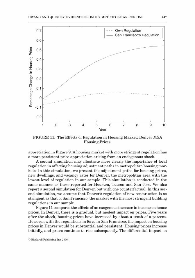
FIGURE 11: The Effects of Regulation in Housing Market: Denver MSAHousing Prices.

appreciation in Figure 9. A housing market with more stringent regulation hasa more persistent price appreciation arising from an endogenous shock.

A second simulation may illustrate more clearly the importance of localregulation in affecting housing adjustment paths in metropolitan housing mar-kets. In this simulation, we present the adjustment paths for housing prices,new dwellings, and vacancy rates for Denver, the metropolitan area with thelowest level of regulation in our sample. This simulation is conducted in thesame manner as those reported for Houston, Tucson and San Jose. We alsoreport a second simulation for Denver, but with one counterfactual. In this sec-ond simulation, we assume that Denver’s regulation of new construction is asstringent as that of San Francisco, the market with the most stringent buildingregulations in our sample.

Figure 11 compares the effects of an exogenous increase in income on houseprices. In Denver, there is a gradual, but modest impact on prices. Five yearsafter the shock, housing prices have increased by about a tenth of a percent.However, with the regulations in force in San Francisco, the impact on housingprices in Denver would be substantial and persistent. Housing prices increaseinitially, and prices continue to rise subsequently. The differential impact on



1 1.5 2 2.5 3 3.5 4 4.5 50

500

1000

1500

2000

2500

Year

Bu

ildin

g P

erm

its

Own Regulation


FIGURE 12: The Effects of Regulation in Housing Market: Denver MSABuilding Permits.

new construction is also substantial. The general pattern appears to be similar;building permits rise upon impact, and return quickly to previous levels. How-ever, under its current regulatory regime, the new supply of housing in Denveris larger by 10 percent than it would be under the more stringent regulationsin effect in San Francisco (Figure 12). Vacancies fall more rapidly with morestringent building regulation (Figure 13). With a lower level of new construc-tion, vacancies would be more responsive to increases in demand. Moreover,as price increases with more stringent regulations, homeowners find it moreexpensive to keep houses vacant.

6. CONCLUSION

This paper estimates the effects of national and regional economic condi-tions on local housing markets using a panel of U.S. metropolitan areas over a14-year period. We estimate the effects of exogenous conditions on the pricesand vacancy rates for owner-occupied single-family housing, and on buildingpermits issued for new construction of single-family housing. The parametersare estimated by two-stage least squares in an error components framework.



1 2 3 4 5 6 7 8 9 102

2.05

2.1

2.15

2.2

2.25

2.3

2.35

2.4

2.45

2.5

Year

Vacancy R

ate

Own Regulation


FIGURE 13: The Effects of Regulation in Housing Market: Denver MSAVacancy Rates.

The empirical models provide a coherent set of empirical and simulationresults. The results confirm the importance of changes in regional economicconditions, income and employment, upon local housing markets, and theyconfirm the importance of lagged adjustment processes on both the demandand supply sides of the market. The results also provide the first detailed ev-idence on the importance of vacancies in the owner-occupied housing marketon housing prices and supplier activity. The results also document the impor-tance of new supply and the factors—variations in materials, labor and capitalcosts, and regulation—affecting decisions to increase the supply of single-familyhousing.

Simulation exercises, using standard impulse response analyses, documentthe lags in market responses to endogenous shocks and the variations in re-sponse predicted from a common model depend greatly upon local conditions.Finally, the results suggest the importance of local regulation in affecting thepattern of market responses to regional economic conditions. In more regulatedmarkets, levels of housing prices are higher in response to endogenous shocks,and the price increases are far more persistent over time.



REFERENCESArnott, Richard. 1989. “Housing Vacancies, Thin Markets, and Idiosyncratic Tastes,” Journal of

Real Estate Finance and Economics, 2, 5–30.Baltagi, Badi. 1981. “Simultaneous Equations with Error Components,” Journal of Econometrics,

17, 189–200.Campbell, John, Andrew Lo, and Craig MacKinlay. 1996. The Econometrics of Financial Markets.

Princeton: Princeton University Press.Clapham, Eric, Peter Englund, John M. Quigley, and Christian Redfearn. 2005. “Revisiting the

Past and Settling the Score: House Price Measurement for Derivative Contracts,” Working Paper05-002, Berkeley Program on Housing and Urban Policy.

Cochrane, John. 1991. “Volatility Tests and Efficient Markets,” Journal of Monetary Economics,27, 463–485.

DiPasquale, Denise. 1999. “Why Don’t We Know More About Housing Supply?” Journal of RealEstate Finance and Economics, 18, 9–23.

DiPasquale, Denise, and William Wheaton. 1994. “Housing Market Dynamics and the Future ofHousing Prices,” Journal of Urban Economics, 35, 1–27.

Dougherty, Ann, and Robert Van Order. 1982. “Inflation, Housing Costs and the Consumer PriceIndex,” American Economic Review, 72, 154–164.

Drieman, Michelle, and Robert Follain. 2003. “Drawing Inferences about Housing Supply Elasticityfrom House Price Responses to Income Shocks,” OFHEO Working Paper 03-02.

Eubank, Arthur, and C. F. Sirmans. 1979. “The Price Adjustment Mechanism for Rental Housingin the United States,” Quarterly Journal of Economics, 93, 163–183.

Evenson, Bengte. 2001. “Understanding House Price Volatility: Measuring and Explaining theSupply Side of Metropolitan Area Housing Markets,” MIT Working Paper.

Follain, James, and Orawin Velz. 1995. “Incorporating the Number of Existing Home Sales into aStructural Model of the Market for Owner-Occupied Housing,” Journal of Housing Economics,4, 93–117.

Gabriel, Stuart, and Frank Nothaft. 1988. “Rental Housing Markets and the Natural VacancyRate,” AREUEA Journal, 16, 419–429.

———. 2001. “Rental Housing Markets, The Incidence and Duration of Vacancy, and the NaturalVacancy Rate,” Journal of Urban Economics, 49, 121–149.

Glaeser, Edward L., Joseph Gyourko, and Raven Saks. 2003. “Why is Manhattan So Expensive?Regulation and the Rise in House Prices,” NBER Working Paper 10124.

Hendershott, Patric H., Bryan MacGregor, and Raymond Tse. 2000. “Estimating the Rental Ad-justment Process,” University of Aberdeen Working Paper.

Hsiao, Cheng. 1986. Analysis of Panel Data. Econometric Society Monograph No. 11, New York:Cambridge University Press.

Hwang, Min, John M. Quigley, and Jae Young Son. 2005. “The Dividend Pricing Model: New Ev-idence from the Korean Housing Market,” Journal of Real Estate Finance and Economics, 32,205–228.

Igarashi, Masahiro. 1992. “The Rent-Vacancy Relationship in the Rental Housing Market,” Journalof Housing Economics, 1, 251–270.

Kearl, James R. 1979. “Inflation, Mortgage, and Housing,” The Journal of Political Economy, 87,1115–1138.

Malpezzi, Stephen. 1996. “Housing Prices, Externalities, and Regulation in the U.S. MetropolitanAreas,” Journal of Housing Research, 7, 209–241.

Malpezzi, Stephen, Gregory Chun, and Richard Green. 1998. “New Place-to-Place Housing PriceIndexes for U.S. Metropolitan Areas and Their Determinants,” Real Estate Economics, 26, 235–274.

Mankiw, N. Gregory, and David N. Weil. 1989. “The Baby Boom, the Baby Bust, and the HousingMarket,” Regional Science and Urban Economics, 19, 235–258.

Mayer, Christopher, and Tsur Somervile. 2000. “Land Use Regulation and New Construction,”Regional Science and Urban Economics, 30, 639–662.



Muth, Richard. 1960. “The Demand for Non-Farm Housing,” in Arnold C. Haberger, Muth Richard,M. L. Burstein, and Gregory C. Chow (eds.), The Demand for Durable Goods. Chicago, IL: Uni-versity of Chicago Press, pp. 26–96.

———. 1968. Cities and Housing. Chicago, IL: University of Chicago Press.Poterba, James M. 1984. “Tax Subsidies to Owner Occupied Housing: An Asset Market Approach,”

Quarterly Journal of Economics, 94, 729–752.———. 1991. “House Price Dynamics: The Role of Tax Policy and Demography,” Brookings Papers

on Economic Activity, 2, 143–183.Quigley, John M., and Larry Rosenthal. 2005. “The Effects of Land Use Regulation on the Price of

Housing: What do We Know? What Can We Learn,” Cityscape, 8, 69–138.Read, Colin. 1993. “Tenants’ Search and Vacancies in Rental Housing Markets,” Regional Science

and Urban Economics, 23, 171–183.———. 1997. “Vacancies and Rent Dispersion in a Stochastic Search Model with Generalized Tenant

Demand,” Journal of Real Estate Finance and Economics, 15, 223–237.Reid, Margaret. 1962. Housing and Income. Chicago, IL: University of Chicago Press.Rosen, Kenneth T., and Lawrence B. Smith. 1983. “The Price Adjustment Process and the Natural

Vacancy Rate,” American Economic Review, 73, 779–786.Rosenthal, Stuart. 1999. “Housing Supply: The Other Half of the Market. A Note from the Editor,”

Journal of Real Estate Finance and Economics, 18, 5–7.Shiller, Robert J. 1981. “Do Stock Prices Move Too Much to be Justified by Subsequent Dividends?”

American Economic Review, 71, 421–436.Topel, Robert, and Sherwin Rosen. 1988. “Housing Investment in the United States,” Journal of

Political Economy, 96, 718–740.U.S. Department of Housing and Urban Development. 1995. “Fair Market Rents for the Section 8

Housing Assistance Payments Program,” Processed.Wheaton, William C. 1990. “Vacancy, Search, and Prices in a Housing Market Matching Model,”

Journal of Political Economy, 98, 1270–1292.

APPENDIX A

Approximation of Equation (3), the Equilibrium Conditionfor Housing Demand

Following Campbell, Lo and MacKinlay (1996),

log(

1 + XY

)= log

(1 + exp

(log

(XY

)))= log (1 + exp(log (X ) − log (Y )))= log (1 + exp(x − y)) ∼= � + �(x − y)

(A1)

Consider Equation (1) in the text. Taking logs on both sides, and using Equa-tion (A1) yields

log (Ht) + log (Dt) = log (St − Vt)

= log (St) + log(

1 − Vt

St

)= log (St) + �1 + �2(log (Vt) − log (St))= �1 + (1 − �2) log (St) + �2 log (Vt)

(A2)



Taking first-order differences in the above expression yields

�log (Ht) + �log (Dt) = (1 − �2)�log (St) + �2�log (Vt)(A3)

Assuming linearity in (2) and solving for p∗ yields expression (3) in the text.

APPENDIX B

Time Aggregation of Expected Housing Price Appreciationand Conditional Variances

This appendix shows how to calculate the expectation and conditional vari-ance of annual housing price appreciation using quarterly observations.

Assume that rt, quarterly housing returns, follows AR(4)-GARCH (1,1),that is,

rt = �0 +4∑

k=1

�krt−k + εt(B1)

where ε t = √htut and ut ∼ iid N(0, 1) and ht = �0 + �1ε2

t−1 + �2ht−1The conditional expectation and volatility of annual housing returns, given

quarterly stochastic process (B1), are

E

(4∑

j=1

rt+ j

∣∣∣∣∣It

)(B2)

and

E

⎡⎣(4∑

j=1

rt+ j − E

(4∑

j=1

rt+ j

∣∣∣∣∣ It

))2∣∣∣∣∣∣ It

⎤⎦(B3)

To calculate expected annual housing price appreciation in (B2), note that

rt+m = E [rt+m | It] +m∑

n=1

�nεt+n = Cm +4∑

l=1

bm,lrt−l+1 +m∑

n=1

�m,nεt+n(B4)

andCm+1 = Cm + bm,1�0

bm+1,l = bm,1�l + bm,l+1 for l < 4

bm+1,4 = bm,1�4

�m+1,1 = bm,1

�m+1,n = �m,n−1 for n> 1

(B5)

Starting m = 1 and iterating over m = 2, 3, and 4, it is easy to compute (B2)using (B4) and (B5).



For the aggregation of conditional variances in housing returns over time,note that

E

⎡⎣(K∑

i=1

rt+i − E

(K∑

i=1

rt+i

∣∣∣∣∣ It

))2∣∣∣∣∣∣ It

⎤⎦= Et

⎡⎣(4∑

m=1

m∑n=1

�m,nεt+n

)2⎤⎦

= Et

[(K∑

m=1

m∑n=1

�m,n

(K∑

s=n�s,n

)(εt+n)2

)]

=K∑

m=1

m∑j=1

�m,n

(K∑

s=n�s,n

)Et

(ε2

t+n

)

(B6)

The term∑K

m=1∑m

j=1 �m,n(∑K

s=n �s,n) can be computed using (B5). ForEt(ε2

t+n), note that

Et(ε2

t+k

) = Et(ht+k) = �0 + �1 Et(ε2

t+k−1

) + �2 Et(ht+k−1)

= �0 + (�1 + �2) (�0 + (�1 + �2) Et (ht+k−2))

=k−1∑h=0

�0 (�1 + �2)h + (�1 + �2)k ht


economic fundamentals in local housing …urbanpolicy.berkeley.edu/pdf/hq_jors06.pdf · changes in...

Documents