United States Office Of Air QualityPlanning And StandardsResearch Triangle Park, NC 27711 FINAL REPORT

EPA-452/R-00-008 Environmental Protection December 2000 Agency

Air

Economic Impact Analysis of Proposed Integrated Iron and Steel

NESHAP

Final Report

Economic Impact Analysis of Proposed Integrated Iron and Steel

NESHAP

U.S. Environmental Protection AgencyOffice of Air Quality Planning and Standards

Innovative Strategies and Economics Group, MD-15Research Triangle Park, NC 27711

Prepared Under Contract By:

Research Triangle InstituteCenter for Economics Research

Research Triangle Park, NC 27711

December 2000

This report has been reviewed by the Emission Standards Division of the Office of Air Quality Planning and Standards of the United States Environmental Protection Agency and approved for publication. Mention of trade names or commercial products is not intended to constitute endorsement or recommendation for use. Copies of this report are available through the Library Services (MD-35), U.S. Environmental Protection Agency, Research Triangle Park, NC 27711, or from the National Technical Information Services 5285 Port Royal Road, Springfield, VA 22161.

CONTENTS

Section Page

1 Introduction . . . . . . . . . . . . . . . . . . . . . . . . . . . . . . . . . . . . . . . . . . . . . . . . . . . . 1-1

1.1 Agency Requirements for an EIA . . . . . . . . . . . . . . . . . . . . . . . . . . . . . 1-1

1.2 Overview of Iron and Steel and Coke Industries . . . . . . . . . . . . . . . . . . 1-2

1.3 Summary of EIA Results . . . . . . . . . . . . . . . . . . . . . . . . . . . . . . . . . . . . 1-2

1.4 Organization of this Report . . . . . . . . . . . . . . . . . . . . . . . . . . . . . . . . . . 1-4

2 Industry Profile . . . . . . . . . . . . . . . . . . . . . . . . . . . . . . . . . . . . . . . . . . . . . . . . . . 2-1

2.1 Production Overview . . . . . . . . . . . . . . . . . . . . . . . . . . . . . . . . . . . . . . . 2-12.1.1 Iron Making . . . . . . . . . . . . . . . . . . . . . . . . . . . . . . . . . . . . . . . . 2-22.1.2 Steel Making . . . . . . . . . . . . . . . . . . . . . . . . . . . . . . . . . . . . . . . 2-52.1.3 Types of Steel Mill Products . . . . . . . . . . . . . . . . . . . . . . . . . . . 2-82.1.4 Emissions . . . . . . . . . . . . . . . . . . . . . . . . . . . . . . . . . . . . . . . . . 2-11

2.2 Industry Organization . . . . . . . . . . . . . . . . . . . . . . . . . . . . . . . . . . . . . . 2-112.2.1 Iron and Steel Making Facilities . . . . . . . . . . . . . . . . . . . . . . . 2-112.2.2 Companies . . . . . . . . . . . . . . . . . . . . . . . . . . . . . . . . . . . . . . . . 2-182.2.3 Industry Trends . . . . . . . . . . . . . . . . . . . . . . . . . . . . . . . . . . . . 2-21

2.3 Uses and Consumers . . . . . . . . . . . . . . . . . . . . . . . . . . . . . . . . . . . . . . 2-22

2.4 Historic Market Data . . . . . . . . . . . . . . . . . . . . . . . . . . . . . . . . . . . . . . 2-242.4.1 Steel Mill Products . . . . . . . . . . . . . . . . . . . . . . . . . . . . . . . . . . 2-242.4.2 Market Prices . . . . . . . . . . . . . . . . . . . . . . . . . . . . . . . . . . . . . . 2-29

2.5 Future Projections . . . . . . . . . . . . . . . . . . . . . . . . . . . . . . . . . . . . . . . . 2-302.5.1 Iron Making . . . . . . . . . . . . . . . . . . . . . . . . . . . . . . . . . . . . . . . 2-302.5.2 Steel Making and Casting . . . . . . . . . . . . . . . . . . . . . . . . . . . . 2-302.5.3 Steel Mill Products . . . . . . . . . . . . . . . . . . . . . . . . . . . . . . . . . . 2-332.5.4 End User Markets . . . . . . . . . . . . . . . . . . . . . . . . . . . . . . . . . . 2-33

iii

3 Engineering Cost Analysis . . . . . . . . . . . . . . . . . . . . . . . . . . . . . . . . . . . . . . . . . 3-1

3.1 Overview of Emissions from Integrated Iron and Steel Plants . . . . . . . 3-1

3.2 Approach for Estimating Compliance Costs . . . . . . . . . . . . . . . . . . . . . 3-2

3.3 BOPF Primary Control Systems . . . . . . . . . . . . . . . . . . . . . . . . . . . . . . 3-2

3.4 Secondary Capture and Control Systems for FugitiveEmissions . . . . . . . . . . . . . . . . . . . . . . . . . . . . . . . . . . . . . . . . . . . . . . . . 3-4

3.5 Bag Leak Detection Systems . . . . . . . . . . . . . . . . . . . . . . . . . . . . . . . . . 3-4

3.6 Total Nationwide Costs . . . . . . . . . . . . . . . . . . . . . . . . . . . . . . . . . . . . . 3-5

4 Economic Impact Analysis . . . . . . . . . . . . . . . . . . . . . . . . . . . . . . . . . . . . . . . . 4-1

4.1 EIA Data Inputs . . . . . . . . . . . . . . . . . . . . . . . . . . . . . . . . . . . . . . . . . . . 4-14.1.1 Producer Characterization . . . . . . . . . . . . . . . . . . . . . . . . . . . . . 4-14.1.2 Market Characterization . . . . . . . . . . . . . . . . . . . . . . . . . . . . . . . 4-24.1.3 Regulatory Control Costs . . . . . . . . . . . . . . . . . . . . . . . . . . . . . . 4-3

4.2 EIA Methodology Summary . . . . . . . . . . . . . . . . . . . . . . . . . . . . . . . . . 4-4

4.3 Economic Impact Results . . . . . . . . . . . . . . . . . . . . . . . . . . . . . . . . . . . . 4-74.3.1 Market-Level Impacts . . . . . . . . . . . . . . . . . . . . . . . . . . . . . . . . 4-74.3.2 Industry-Level Impacts . . . . . . . . . . . . . . . . . . . . . . . . . . . . . . . . 4-8

4.3.2.1 Changes in Profitability . . . . . . . . . . . . . . . . . . . . . . . 4-94.3.2.2 Facility Closures . . . . . . . . . . . . . . . . . . . . . . . . . . . . 4-114.3.2.3 Changes in Employment . . . . . . . . . . . . . . . . . . . . . . 4-11

4.3.3 Social Cost . . . . . . . . . . . . . . . . . . . . . . . . . . . . . . . . . . . . . . . . 4-13

5 Small Business Impacts . . . . . . . . . . . . . . . . . . . . . . . . . . . . . . . . . . . . . . . . . . . 5-1

References . . . . . . . . . . . . . . . . . . . . . . . . . . . . . . . . . . . . . . . . . . . . . . . . . . . . . . . . . . . R-1

Appendixes

A Economic Impact Analysis Methodology . . . . . . . . . . . . . . . . . . . . . . . . . . . . A-1

B Development of Coke Battery Cost Functions . . . . . . . . . . . . . . . . . . . . . . . . . . B-1

C Econometric Estimation of the Demand Elasticity for Steel MillProducts . . . . . . . . . . . . . . . . . . . . . . . . . . . . . . . . . . . . . . . . . . . . . . . . . . . . . . . C-1

iv

D Joint Economic Impact Analysis of the Integrated Iron and SteelMACT Standard with the Coke MACT Standard . . . . . . . . . . . . . . . . . . . . . . D-1

v

LIST OF FIGURES

Number Page

1-1 Summary of Interactions Between Producers and Commodities in theIron and Steel Industry . . . . . . . . . . . . . . . . . . . . . . . . . . . . . . . . . . . . . . . . . . . . 1-3

2-1 Overview of the Integrated Steel Making Process . . . . . . . . . . . . . . . . . . . . . . . 2-22-2 Iron Making Process: Blast Furnace . . . . . . . . . . . . . . . . . . . . . . . . . . . . . . . . . 2-42-3 Steel Making Processes: Basic Oxygen Furnace and Electric Arc

Furnace . . . . . . . . . . . . . . . . . . . . . . . . . . . . . . . . . . . . . . . . . . . . . . . . . . . . . . . . 2-62-4 Steel Casting Processes: Ingot Casting and Continuous Casting . . . . . . . . . . . 2-82-5 U.S. Raw Steel Production Shares by Type of Steel: 1997 . . . . . . . . . . . . . . . 2-92-6 Steel Finishing Processes by Mill Type . . . . . . . . . . . . . . . . . . . . . . . . . . . . . . 2-102-7 Location of U.S. Integrated Iron and Steel Manufacturing Plants: 1997 . . . . 2-122-8 1997 U.S. Steel Shipments by Market Classification . . . . . . . . . . . . . . . . . . . 2-23

4-1 Market Linkages Modeled in the Economic Impact Analysis . . . . . . . . . . . . . . 4-34-2 Market Equilibrium without and with Regulation . . . . . . . . . . . . . . . . . . . . . . . 4-6

vi

LIST OF TABLES

Number Page

2-1 Summary Data for Integrated Iron and Steel Facilities: 1997 (shorttons per year) . . . . . . . . . . . . . . . . . . . . . . . . . . . . . . . . . . . . . . . . . . . . . . . . . . 2-13

2-2 Summary of Steel Making Operations at Integrated Iron and SteelFacilities: 1997 (short tons per year) . . . . . . . . . . . . . . . . . . . . . . . . . . . . . . . . 2-14

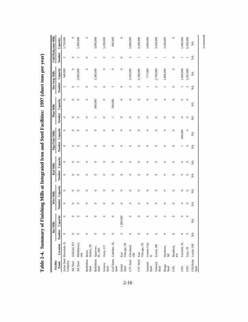
2-3 U.S. Steel Making Capacity and Utilization: 1981-1997 . . . . . . . . . . . . . . . . 2-152-4 Summary of Finishing Mills at Integrated Iron and Steel Facilities:

1997 (short tons per year) . . . . . . . . . . . . . . . . . . . . . . . . . . . . . . . . . . . . . . . . 2-162-5 Integrated Iron and Steel Industry Summary Data: 1997 . . . . . . . . . . . . . . . . 2-192-6 Summary of Integrated Iron and Steel Operations at U.S. Parent

Companies: 1997 (short tons per year) . . . . . . . . . . . . . . . . . . . . . . . . . . . . . . 2-202-7 Sales, Operating Income, and Profit Rate for Integrated Producers and

Mini-Mills: 1996 . . . . . . . . . . . . . . . . . . . . . . . . . . . . . . . . . . . . . . . . . . . . . . . 2-212-8 Comparison of Steel and Substitutes by Cost, Strength, and

Availability: 1997 . . . . . . . . . . . . . . . . . . . . . . . . . . . . . . . . . . . . . . . . . . . . . . 2-252-9 Net Shipments of Steel Mill Products by Market Classification:

1981-1997 (103 short tons) . . . . . . . . . . . . . . . . . . . . . . . . . . . . . . . . . . . . . . . . 2-262-10 U.S. Production, Foreign Trade, and Apparent Consumption of Steel

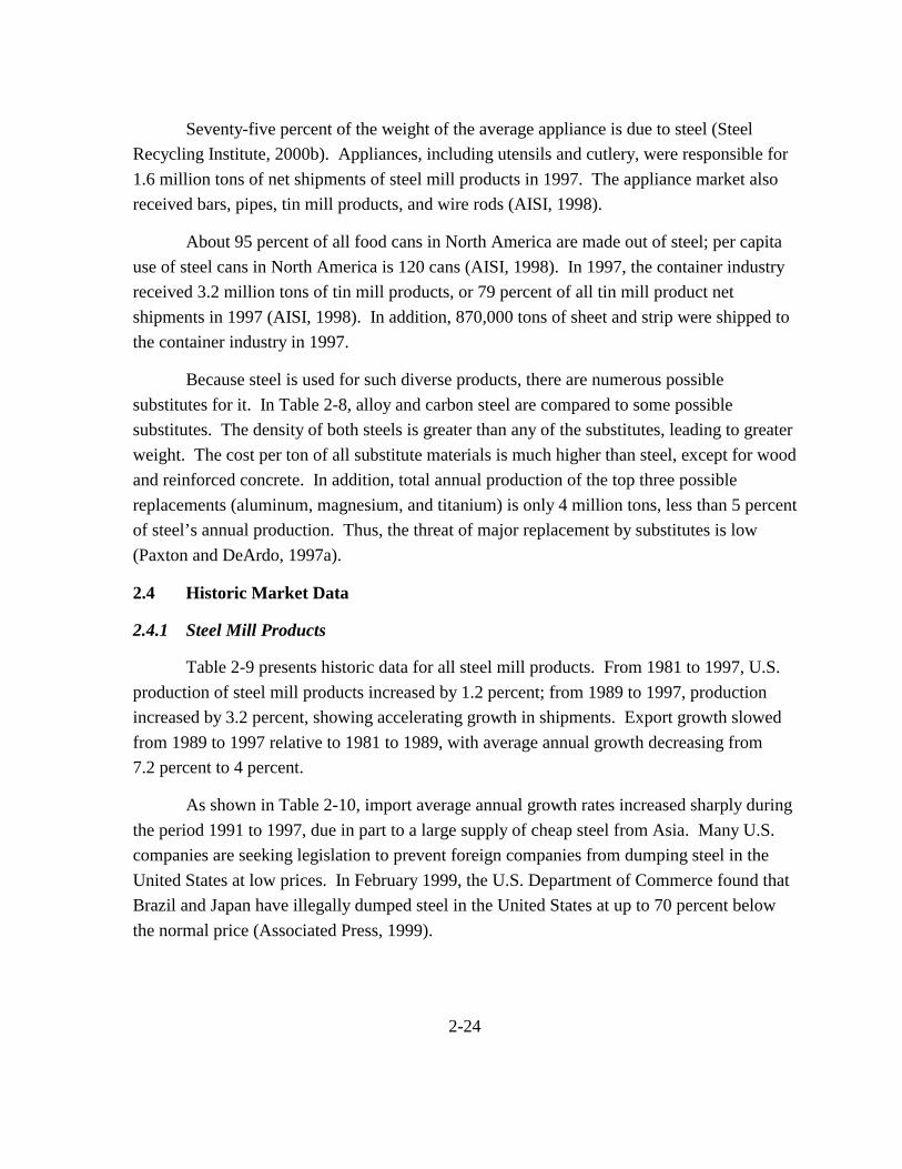
Mill Products: 1981-1997 (103 short tons) . . . . . . . . . . . . . . . . . . . . . . . . . . . 2-272-11 Foreign Trade Concentration Ratios for U.S. Steel Mill Products:

1981-1997 . . . . . . . . . . . . . . . . . . . . . . . . . . . . . . . . . . . . . . . . . . . . . . . . . . . . 2-282-12 U.S. Production, Foreign Trade, and Apparent Consumption of Steel

Mill Products: 1997 (tons) . . . . . . . . . . . . . . . . . . . . . . . . . . . . . . . . . . . . . . . . 2-292-13 Market Prices and Net Shipments of Steel Mill Products by Steel

Type: 1997 . . . . . . . . . . . . . . . . . . . . . . . . . . . . . . . . . . . . . . . . . . . . . . . . . . . 2-312-14 Projected U.S. Production, Foreign Trade, and Apparent Consumption

of Steel Mill Products: 1994, 1999, and 2004 (103 short tons) . . . . . . . . . . . . 2-322-15 Projected U.S. Apparent Consumption of Steel Mill Product by Type:

1994, 1999, and 2004 (103 short tons) . . . . . . . . . . . . . . . . . . . . . . . . . . . . . . . 2-322-16 Apparent Consumption of Steel By-Products: 1994-2004 (103

net tons) . . . . . . . . . . . . . . . . . . . . . . . . . . . . . . . . . . . . . . . . . . . . . . . . . . . . . . 2-332-17 Apparent Steel Consumption for Selected End Users: 1994-2004

(103 net tons) . . . . . . . . . . . . . . . . . . . . . . . . . . . . . . . . . . . . . . . . . . . . . . . . . . 2-34

vii

2-18 Steel Imports by End-Use Markets: 1994-2004 (103 net tons) . . . . . . . . . . . . 2-362-19 Demand Forecast for Raw Materials in Motor Vehicles: 1992, 1996,

and 2000 (metric tons) . . . . . . . . . . . . . . . . . . . . . . . . . . . . . . . . . . . . . . . . . . . 2-37

3-1 Nationwide Cost Estimates . . . . . . . . . . . . . . . . . . . . . . . . . . . . . . . . . . . . . . . . 3-5

4-1 Baseline Characterization of U.S. Iron and Steel Markets: 1997 . . . . . . . . . . . 4-44-2 Supply and Demand Elasticities Used in Analysis . . . . . . . . . . . . . . . . . . . . . . 4-84-3 Market-Level Impacts of the Proposed Integrated Iron and Steel

MACT: 1997 . . . . . . . . . . . . . . . . . . . . . . . . . . . . . . . . . . . . . . . . . . . . . . . . . . . 4-94-4 National-Level Industry Impacts of the Proposed Integrated Iron and

Steel MACT: 1997 . . . . . . . . . . . . . . . . . . . . . . . . . . . . . . . . . . . . . . . . . . . . . 4-104-5 Distribution Impacts of the Proposed Integrated Iron and Steel MACT

Across Directly Affected Producers: 1997 . . . . . . . . . . . . . . . . . . . . . . . . . . . 4-124-6 Distribution of the Social Costs of the Proposed Integrated Iron and

Steel MACT: 1997 . . . . . . . . . . . . . . . . . . . . . . . . . . . . . . . . . . . . . . . . . . . . . 4-14

viii

SECTION 1

INTRODUCTION

The U.S. Environmental Protection Agency (EPA) is developing a maximum achievable control technology (MACT) standard to reduce hazardous air pollutants (HAPs) from the integrated iron and steel manufacturing source category. To support this rulemaking, EPA’s Innovative Strategies and Economics Group (ISEG) has conducted an economic impact analysis (EIA) to assess the potential costs of the rule. This report documents the methods and results of this EIA. In 1997, the United States produced a total of 105.9 million short tons of steel mill products. The construction and automotive industries are two of the largest consumers of these products, consuming approximately 30 percent of the net shipments in that year. The processes covered by this proposed regulation include sinter production, iron production in blast furnaces, and basic oxygen process furnace (BOPF) shops. There are a variety of metal and organic HAPs contained in the particulate matter emitted from these iron and steel manufacturing processes. Metal HAPs include primarily manganese and lead, while volatile organics include benzene, carbon disulfide, toluene, and xylene.

1.1 Agency Requirements for an EIA

Congress and the Executive Office have imposed statutory and administrative requirements for conducting economic analyses to accompany regulatory actions. Section 317 of the CAA specifically requires estimation of the cost and economic impacts for specific regulations and standards proposed under the authority of the Act.1 EPA’s Economic Analysis Resource Document provides detailed guidelines and expectations for economic

1In addition, Executive Order (EO) 12866 requires a more comprehensive analysis of benefits and costs for proposed significant regulatory actions. Office of Management and Budget (OMB) guidance under EO 12866 stipulates that a full benefit-cost analysis is required only when the regulatory action has an annual effect on the economy of $100 million or more. Other statutory and administrative requirements include examination of the composition and distribution of benefits and costs. For example, the Regulatory Flexibility Act (RFA), as amended by the Small Business Regulatory Enforcement and Fairness Act of 1996 (SBREFA), requires EPA to consider the economic impacts of regulatory actions on small entities.

1-1

analyses that support MACT rulemaking (EPA, 1999). In the case of the integrated iron and steel MACT, these requirements are fulfilled by examining the following:

` facility-level impacts (e.g., changes in output rates, profitability, and facility closures),

` market-level impacts (e.g., changes in market prices, domestic production, and imports),

` industry-level impacts (e.g., changes in revenue, costs, and employment), and

` societal-level impacts (e.g., estimates of the consumer burden as a result of higher prices and reduced consumption levels and changes in domestic and foreign profitability).

1.2 Overview of Iron and Steel and Coke Industries

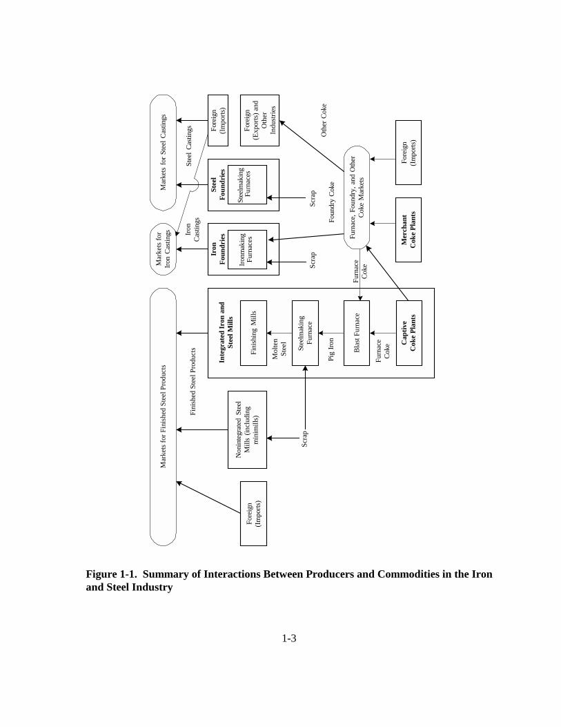
Integrated iron and steel mills are co-located with captive coke plants providing furnace coke for its blast furnaces, while merchant coke plants supply the remaining demand for furnace coke at integrated iron and steel mills. These integrated mills compete with nonintegrated mills (i.e., mini-mills) and foreign imports in the markets for these steel products typically consumed by the automotive, construction, and other durable goods producers. Figure 1-1 summarizes the interactions between source categories and markets within the broader iron and steel industry.

The EIA models the specific links between these models. The analysis to support the integrated iron and steel EIA focuses on two specific markets:

` steel mill products and

` furnace coke.

Changes in price and quantity in these markets are used to estimate the facility, market, industry, and social impacts of the integrated iron and steel regulation.

1.3 Summary of EIA Results

The proposed MACT will cover the integrated iron and steel manufacturing source category. The processes covered by the proposed regulation include sinter production; iron production in blast furnaces; and basic oxygen process furnace (BOPF) shops, which includes hot metal transfer, slag skimming, steelmaking in BOPFs, and ladle metallurgy. Capital, operating and maintenance, and monitoring costs were estimated for each plant.

1-2

Fore

ign

(Exp

orts

) and

O

ther

In

dust

ries

Ironm

akin

gFu

rnac

es

Non

inte

grat

ed S

teel

M

ills

(incl

udin

g m

inim

ills)

Fi

nish

ing

Mill

sFo

reig

n (Im

ports

)

Bla

st F

urna

ce

Mer

chan

t C

oke

Plan

ts

Fore

ign

(Impo

rts)

Fore

ign

(Impo

rts)

Stee

lmak

ing

Furn

ace

Furn

ace

Cok

e

Pig

Iron

Scra

p

Foun

dry

Cok

e O

ther

Cok

e

Mol

ten

Stee

l

Mar

kets

for F

inis

hed

Stee

l Pro

duct

s

Furn

ace

Coke

Mar

kets

for

Iron

Cas

tings

M

arke

ts fo

r Ste

el C

astin

gs

Stee

lmak

ing

Furn

aces

Inte

grat

ed Ir

on a

nd

Stee

l Mill

s

Scra

p

Stee

l Cas

tings

Iron

C

astin

gs

Iron

Fo

undr

ies

Stee

l Fo

undr

ies

Fini

shed

Ste

el P

rodu

cts

Furn

ace,

Fou

ndry

, and

Oth

er

Coke

Mar

kets

Scra

p

Cap

tive

Cok

e Pl

ants

Figure 1-1. Summary of Interactions Between Producers and Commodities in the Iron and Steel Industry

1-3

The increased production costs will lead to economic impacts in the form of small increases in market prices and decreases in domestic production. The impacts of these price increases will be borne largely by integrated producers of steel mill products as well as consumers of steel mill products. Nonintegrated steel mills will earn higher profits. Key results of the EIA for the integrated iron and steel MACT are as follows:

` Engineering Costs: The engineering analysis estimates annual costs for existing sources of $5.9 million.

` Price and Quantity Impacts: The EIA model predicts the following:

— The market price for steel mill products is projected to only slightly increase by less than 0.01 percent ($0.01/short ton), and domestic steel mill production is projected to decrease by less than 0.01 percent (2.3 thousand tons/year).

— The market price for furnace coke is projected to remain unchanged, and domestic furnace coke production is projected to decrease by less than 0.1 percent (100 tons/year).

` Plant Closures: No integrated iron and steel mills or coke batteries are projected to close as a result of the rule.

` Small Businesses: The Agency has determined that no small businesses in this source category would be subject to this proposed rule.

` Social Costs: The annual social costs are projected to be $5.9 million.

— The consumer burden as a result of higher prices and reduced consumption levels is $1.7 million annually.

— The aggregate producer profits are expected to decrease by $4.2 million.

q The profit losses are $5.2 million annually for domestic integrated iron and steel producers.

q Unaffected domestic producers and foreign producer profits increase by $0.9 million due to higher prices and level of impacts.

1.4 Organization of this Report

The remainder of this report supports and details the methodology and the results of the EIA of the integrated iron and steel MACT.

` Section 2 presents a profile of the integrated iron and steel industry.

1-4

` Section 3 describes the regulatory controls and presents engineering cost estimates for the regulation.

` Section 4 reports market-, industry-, and societal-level impacts.

` Section 5 contains the small business screening analysis.

` Appendix A describes the EIA methodology.

` Appendix B describes the development of the coke battery cost functions.

` Appendix C includes the econometric estimation of the demand elasticity for steel mill products.

` Appendix D reports the results of the joint economic impacts of the iron and steel and coke MACTs.

1-5

SECTION 2

INDUSTRY PROFILE

Iron is produced from iron ore, and steel is produced by progressively removing impurities from iron ore or ferrous scrap. Iron and steel manufacture is included under Standard Industrial Classification (SIC) code 3312—Blast Furnaces and Steel Mills, which also includes the production of coke, an input to the iron making process. In 1997, the United States produced 105.9 million short tons of steel. Steel is primarily used as a major input to consumer products such as automobiles and appliances. Therefore, the demand for steel is a derived demand that depends on a diverse base of consumer products.

This section provides a summary profile of the integrated iron and steel industry in the United States. Technical and economic aspects of the industry are reviewed to provide background for the economic impact analysis. Section 2.1 provides an overview of the production processes and the resulting types of steel mill products. Section 2.2 summarizes the organization of the U.S. integrated iron and steel industry, including a description of the U.S. integrated iron and steel mills, the companies that own these facilities, and the markets for steel mill products. Section 2.3 describes uses and consumers. Section 2.4 presents historical and projected data on the iron and steel industry, including U.S. production, consumption, and foreign trade. Finally, Section 2.5 discusses future projections.

2.1 Production Overview

Figure 2-1 illustrates the four-step production process for the manufacture of steel products at integrated iron and steel mills. The first step is iron making. Primary inputs to the iron making process are iron ore or other sources of iron, coke or coal, and flux. Pig iron is the primary output of iron making and the primary input to the next step in the process, steel making. Metal scrap and flux are also used in steel making. The steel making process produces molten steel that is shaped into solid forms at forming mills. Finishing mills then shape, harden, and treat the semi-finished steel to yield its final marketable condition.

2-1

Iron Ore Coke Flux

Scrap Flux

Finished Steel Products

Figure 2-1. Overview of the Integrated Steel Making Process

2.1.1 Iron Making

Blast furnaces are the primary site of iron making at integrated facilities where iron ore is converted into more pure and uniform iron. Blast furnaces are tall steel vessels lined with heat-resistant brick (AISI, 1989a). They range in size from 23 to 45 feet in diameter and are over 100 feet tall (Hogan and Kolble, 1996; Lankford et al., 1985). Conveyor systems of carts and ladles carry inputs and outputs to and from the blast furnace.

Iron ore, coke, and flux are the primary inputs to the iron making process. Iron ore, which is typically 50 to 70 percent iron, is the primary source of iron for integrated iron and

2-2

Steel Making

Iron Making

Molten Steel

Pig Iron

Forming

Finishing

Semi-Finished Steel

steel mills. Pellets are the primary source of iron ore used in iron making at integrated steel mills. Iron can also be captured by sintering from fine grains, pollution control dust, and sludge. Sintering ignites these materials and fuses them into cakes that are 52 to 60 percent iron. Other iron sources are scrap metal, mill scale, and steel making slag that is 20 to 25 percent iron (Lankford et al., 1985).

Coke is made in ovens that heat metallurgical coal to drive off gases, oil, and tar, which can be collected by a coke by-product plant to use for other purposes or to sell. Coke may be generated by an integrated iron and steel facility or purchased from a merchant coke producer. Iron makers are exploring techniques that directly use coal to make iron, thereby eliminating the need to first make coke. Coke production is responsible for 72 percent of the particulates released in the manufacture of steel products (Prabhu and Cilione, 1992).

Flux is a general name for any material used in the iron or steel making process that is used to collect impurities from molten metal. The most widely used flux is lime. Limestone is also directly used as a flux, but it reacts more slowly than lime (Fenton, 1996).

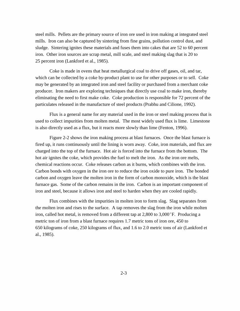
Figure 2-2 shows the iron making process at blast furnaces. Once the blast furnace is fired up, it runs continuously until the lining is worn away. Coke, iron materials, and flux are charged into the top of the furnace. Hot air is forced into the furnace from the bottom. The hot air ignites the coke, which provides the fuel to melt the iron. As the iron ore melts, chemical reactions occur. Coke releases carbon as it burns, which combines with the iron. Carbon bonds with oxygen in the iron ore to reduce the iron oxide to pure iron. The bonded carbon and oxygen leave the molten iron in the form of carbon monoxide, which is the blast furnace gas. Some of the carbon remains in the iron. Carbon is an important component of iron and steel, because it allows iron and steel to harden when they are cooled rapidly.

Flux combines with the impurities in molten iron to form slag. Slag separates from the molten iron and rises to the surface. A tap removes the slag from the iron while molten iron, called hot metal, is removed from a different tap at 2,800 to 3,000bF. Producing a metric ton of iron from a blast furnace requires 1.7 metric tons of iron ore, 450 to 650 kilograms of coke, 250 kilograms of flux, and 1.6 to 2.0 metric tons of air (Lankford et al., 1985).

2-3

Coke

Iron ore

Flux

Air

Pig Iron

Blast Furnace

Dust

Coal or natural gas

Slag

Figure 2-2. Iron Making Process: Blast Furnace

Source: U.S. Environmental Protection Agency, Office of Compliance. 1995. EPA Office of Compliance Sector Notebook Project: Profile of the Iron and Steel Industry. Washington, DC: Environmental Protection Agency.

Hot metal may be transferred directly to steel making furnaces. Hot metal that has cooled and solidified is called pig iron. Pig iron is at least 90 percent iron and 3 to 5 percent carbon (Lankford et al., 1985). Pig iron is typically used in steel making furnaces, but it also may be cast for sale as merchant pig iron. Merchant pig iron may be used by foundries or electric arc furnace (EAF) facilities that do not have iron making capabilities. In 1997, blast furnaces in the United States produced 54.7 million short tons of iron, of which 1.2 percent was sold for use outside of integrated iron and steel mills. Six thousand tons of pig iron were used for purposes other than steel making (AISI, 1998).

2-4

2.1.2 Steel Making

Steel making is carried out in basic oxygen furnaces or in EAFs, while iron making is only carried out in blast furnaces. Basic oxygen furnaces are the standard steel making furnace used at integrated mills, although two facilities use EAFs. EAFs are the standard furnace at mini-mills since they use scrap metal efficiently on a small scale. Open hearth furnaces were used to produce steel prior to 1991 but have not been used in the United States since that time.

Hot metal or pig iron is the primary input to the steel making process at integrated mills. Hot metal accounts for up to 80 percent of the iron charged into a steel making furnace (AISI, 1989a). Scrap metal is also used, which either comes as wastes from other mill activities or is purchased on the scrap metal market. Scrap metal must be carefully sorted to control the alloy content of the steel. Direct-reduced iron (DRI) may also be used to increase iron content, particularly in EAFs that use mainly scrap metal for the iron source. DRI is iron that has been formed from iron ore by a chemical process, directly removing oxygen atoms from the iron oxide molecules.

Predictions for iron sources for basic oxygen furnaces in the year 2004 indicate an expected decrease in the use of pig iron and expected increases in the use of scrap and DRI. Shares for basic oxygen furnaces in 2004 are predicted to be 67 percent pig iron, 27 percent scrap, and 6 percent DRI. In contrast, shares for EAFs in 2004 are predicted to be 2 percent pig iron, 88 percent scrap, and 10 percent DRI (Dun & Bradstreet, 1998).

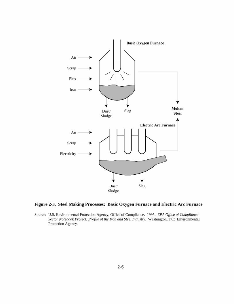
Figure 2-3 shows the steel making process at basic oxygen furnaces and EAFs. At basic oxygen furnaces, hot metal and other iron sources are charged into the furnace. An oxygen lance is lowered into the furnace to inject high purity oxygen—99.5 to 99.8 percent pure—to minimize the introduction of contaminants. Some basic oxygen furnaces insert the oxygen from below. Energy for the melting of scrap and cooled pig iron comes from the oxidation of silicon, carbon, manganese, and phosphorous. Flux is added to collect the oxides produced in the form of slag and to reduce the levels of sulfur and phosphorous in the metal. Approximately 365 kilograms of lime are needed to produce a metric ton of steel (AISI, 1989a). The basic oxygen process can produce approximately 300 tons in 45 minutes (AISI, 1989a). When the process is complete, the furnace is tipped and the molten steel flows out of a tap into a ladle.

2-5

Air

Scrap

Flux

Iron

Air

Scrap

Electricity

Basic Oxygen Furnace

Molten

Sludge

Electric Arc Furnace

Dust/ Slag Steel

Dust/ Slag Sludge

Figure 2-3. Steel Making Processes: Basic Oxygen Furnace and Electric Arc Furnace

Source: U.S. Environmental Protection Agency, Office of Compliance. 1995. EPA Office of Compliance Sector Notebook Project: Profile of the Iron and Steel Industry. Washington, DC: Environmental Protection Agency.

2-6

EAFs have removable roofs so that they can be charged from the top. EAFs primarily use scrap metal for the iron source, but alloys may also be added before the melt. In EAFs, electric arcs are formed between two or three carbon electrodes. The EAFs require a power source to supply the charge necessary to generate the electric arc and typically use electricity purchased from an outside source. If electrodes are aligned so that the current passes above the metal, the metal is heated by radiation from the arc. If the electrodes are aligned so that the current passes through the metal, heat is generated by the resistance of the metal in addition to the arc radiation. Flux is blown or deposited on top of the metal after it has melted. Impurities are oxidized by the air in the furnace and oxygen injections. The melted steel should have a carbon content of 0.15 to 0.25 percent greater than desired because the excess will escape as carbon monoxide as the steel boils. The boiling action stirs the steel to give it a uniform composition. When complete, the furnace is tilted so that the molten steel can be drained through a tap. The slag may be removed from a separate tap. The EAF process takes 2 to 3 hours to complete (EPA, 1995).

Steel often undergoes additional, referred to as secondary, metallurgical processes after it is removed from the steel making furnace. Secondary steel making takes place in vessels, smaller furnaces, or the ladle. These sites do not have to be as strong as the primary refining furnaces because they are not required to contain the powerful primary processes. Secondary steel making can have many purposes, such as removal of oxygen, sulfur, hydrogen, and other gases by exposing the steel to a low-pressure environment; removal of carbon monoxide through the use of deoxidizers such as aluminum, titanium, and silicon; and changing of the composition of unremovable substances such as oxides to further improve mechanical properties.

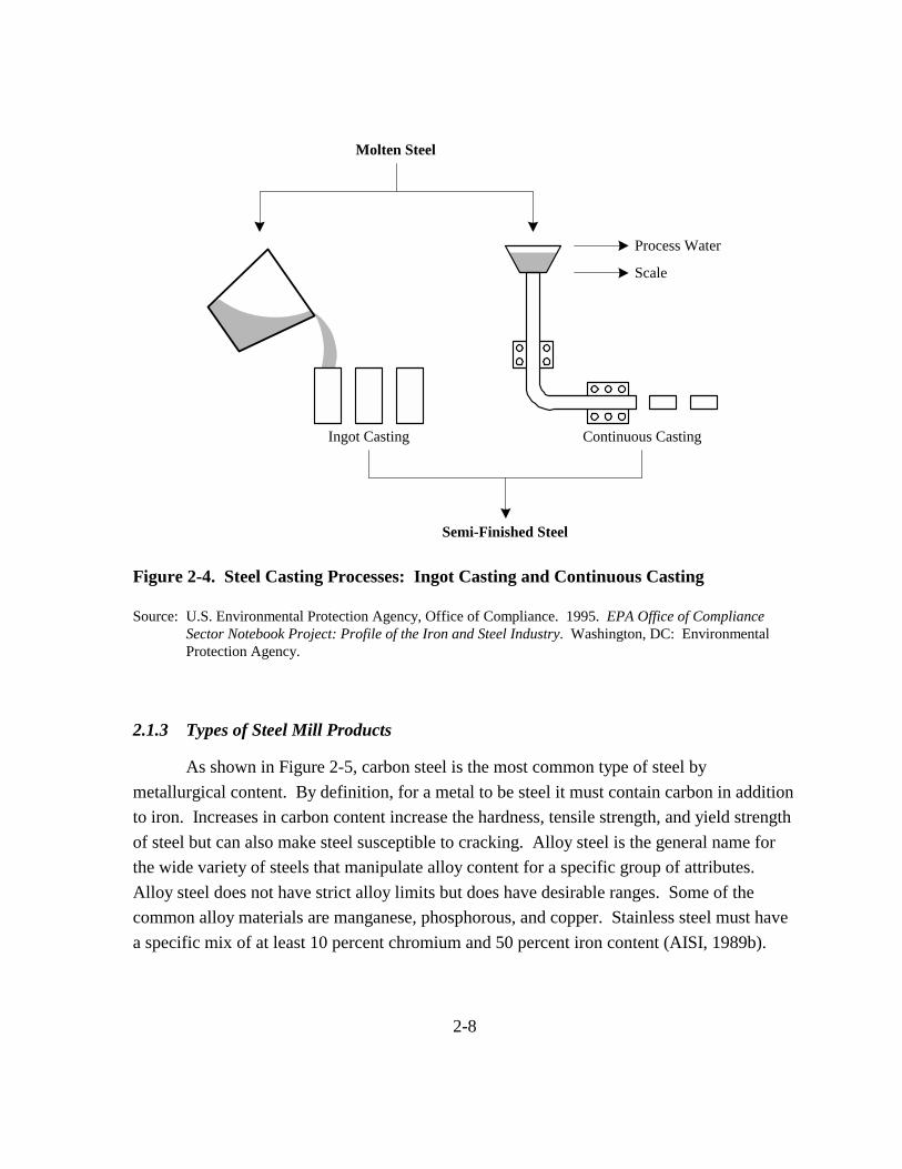
Molten steel transferred directly from the steel making furnace is the primary input to the forming process. Forming must be done quickly before the molten steel begins to cool and solidify. Two generalized methods are used to shape the molten steel into a solid form for use at finishing mills: ingot casting and continuous casting machines (Figure 2-4). Ingot casting is the traditional method of forming molten steel in which the metal is poured into ingot molds and allowed to cool and solidify. However, continuous casting currently accounts for approximately 95 percent of forming operations (AISI, 1998). Continuous casting, in which the steel is cast directly into a moving mold on a machine, reduces loss of steel in processing up to 12 percent over ingot pouring (USGS, 1998). Continuous casting is projected to account for nearly 100 percent of steel mill casting by the year 2004 (Dun & Bradstreet, 1998).

2-7

Molten Steel

Process Water

Scale

Ingot Casting Continuous Casting

Semi-Finished Steel

Figure 2-4. Steel Casting Processes: Ingot Casting and Continuous Casting

Source: U.S. Environmental Protection Agency, Office of Compliance. 1995. EPA Office of Compliance Sector Notebook Project: Profile of the Iron and Steel Industry. Washington, DC: Environmental Protection Agency.

2.1.3 Types of Steel Mill Products

As shown in Figure 2-5, carbon steel is the most common type of steel by metallurgical content. By definition, for a metal to be steel it must contain carbon in addition to iron. Increases in carbon content increase the hardness, tensile strength, and yield strength of steel but can also make steel susceptible to cracking. Alloy steel is the general name for the wide variety of steels that manipulate alloy content for a specific group of attributes. Alloy steel does not have strict alloy limits but does have desirable ranges. Some of the common alloy materials are manganese, phosphorous, and copper. Stainless steel must have a specific mix of at least 10 percent chromium and 50 percent iron content (AISI, 1989b).

2-8

U.S. Raw Steel Production 108.6 million short tons

Carbon 88.4

Alloy 9.4

Stainless 2.2

Figure 2-5. U.S. Raw Steel Production Shares by Type of Steel: 1997

Source: American Iron and Steel Institute (AISI). 1998. Annual Statistical Report. Washington, DC: American Iron and Steel Institute.

Semi-finished steel forms from the casting process are passed through processing lines at finishing mills to give the steel its final shape (Figure 2-6). At rolling mills, steel slabs are flattened or rolled into pipes. At hot strip mills, slabs pass between rollers until they have reached the desired thickness. The slabs may then be cold rolled in cold reduction mills. Cold reduction, which applies greater pressure than the hot rolling process, improves mechanical properties, machinability, and size accuracy, and produces thinner gauges than possible with hot rolling alone. Cold reduction is often used to produce wires, tubes, sheet and strip steel products. In 1997, the United States shipped 19 million tons of hot rolled sheet and strip and over 14 million tons of cold rolled sheet and strip (AISI, 1998).

After the shape and surface quality of steel have been refined at finishing mills, the metal often undergoes further processes for cleansing. Pressurized air or water and cleaning agents are the first step in cleansing. Acid baths during the pickling process remove rust, scales from processing, and other materials. The cleaning and pickling processes help coatings to adhere to the steel. Metallic coatings are frequently applied to sheet and strip to inhibit corrosion and oxidation, and to improve visual appearance. The most common coating is galvanizing, which is a zinc coating. In 1997, the United States had net shipments of over 16 million tons of galvanized sheet and strip (AISI, 1998). Other coatings include

2-9

Figure 2-6. Steel Finishing Processes by Mill Type

Source: Lankford, William T., Norman L. Samways, Robert F. Craven, and Harold E. McGannon, eds. 1985. The Making, Shaping and Treating of Steel. Pittsburgh: United States Steel, Herbick & Held.

aluminum, tin, chromium, and lead, which together accounted for 2 million tons of U.S. net shipments in 1997 (AISI, 1998). Semi-finished products are also finished into pipes and tubes. Pipes are produced by piercing a rod of steel to create a pipe with no seam or by rolling and welding sheet metal.

Slag is generated by iron and steel making. Slag contains the impurities of the molten metal, but it can be sintered to capture the iron content. Slag can also be sold for use by the cement industry, for railroad ballast, and by the construction industry, although steel making slag is not used for these purposes as often as iron making slag (EPA, 1995).

2-10

2.1.4 Emissions

Emissions are generated from numerous points throughout the integrated steel mill production processes. Blast furnace gas, such as carbon monoxide, is often used to heat the air incoming to the blast furnace and can also be used as fuel if it is first cleaned. The iron making process often generates other gases from impurities such as sulfur dioxide or hydrogen sulfide.

Particulates may be included in the blast furnace gas. The steel making process also generates gases that typically contain metallic dust such as iron particulates, zinc, and lead. In addition, when the steel is poured, fumes are released that contain iron oxide and graphite. Air filters and wet scrubbers of emissions generate dust and sludge.

About a thousand gallons of water are used per ton of steel to cleanse emissions (EPA, 1995). The water used to cool and rinse the steel picks up lubricants, cleansers, mill scale, and acids. A sludge may form that contains metals such as cadmium, chromium, and lead.

2.2 Industry Organization

This section provides an overview of the U.S. integrated iron and steel mill industry, including the facilities, the companies that own them, and the markets in which they compete.

2.2.1 Iron and Steel Making Facilities

Figure 2-7 identifies the location of U.S. integrated iron and steel facilities. As of 1997, there were 20 operating integrated steel facilities. Five facilities are located in Ohio, four are in Indiana, two each are in Illinois, Alabama, and Michigan, and one each is in Kentucky, Maryland, Utah, Pennsylvania, and West Virginia.

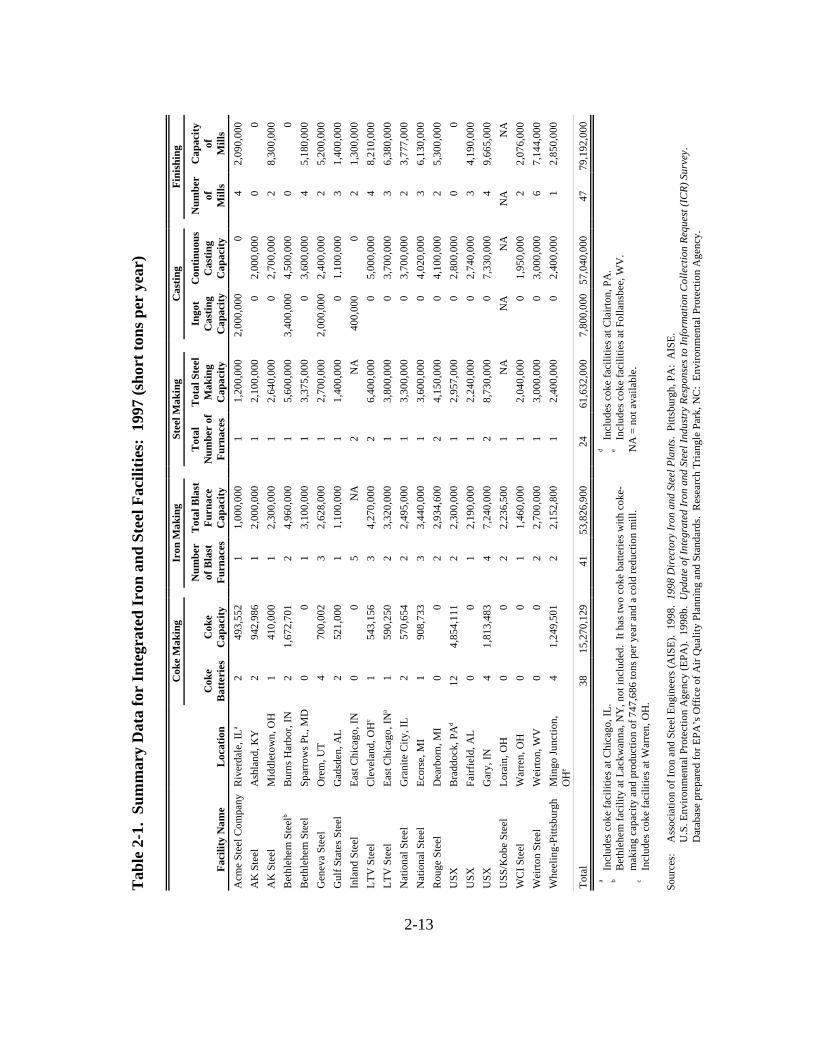
Table 2-1 lists the facilities and their operations. All facilities have iron making, steel making, and casting operations. Thirteen of the facilities have their own coke making operations and 17 have finishing mills. Wherever two plants were considered as one facility, it has been noted.

Table 2-1 also shows all blast furnaces operating in 1997. Forty-one blast furnaces are shown, with an average capacity of 1.4 million tons per year. Individual facility capacity ranges from 1 million tons per year to 4.96 million tons per year.

2-11

Figure 2-7. Location of U.S. Integrated Iron and Steel Manufacturing Plants: 1997

Source: Association of Iron and Steel Engineers (AISE). 1998. 1998 Directory Iron and Steel Plants. Pittsburgh, PA: AISE.

Table 2-2 shows the facilities by furnace type. Twenty-two steel making facilities have basic oxygen furnaces, while only two facilities have EAFs: Inland Steel and Rouge Steel. Total basic oxygen capacity at integrated mills is 60.8 million tons per year, while the EAF capacity is 1.5 million tons per year. Average basic oxygen furnace capacity is 2.8 million tons per year, while average EAF capacity is 725,000 tons per year. Table 2-3 shows steel making capacity and capacity use over time for the United States. Capacity decreased from 1981 to 1988 and again from 1991 to a low in 1994. Capacity increased each year from 1994 to 1997, while capacity utilization decreased over this same period.

2-12

Tabl

e 2-

1. S

umm

ary

Dat

a fo

r In

tegr

ated

Iron

and

Ste

el F

acili

ties:

199

7 (s

hort

tons

per

yea

r)

Cok

e M

akin

g Ir

on M

akin

g St

eel M

akin

g C

astin

g Fi

nish

ing

Num

ber

Tot

al B

last

T

otal

T

otal

Ste

el

Ingo

t C

ontin

uous

N

umbe

r C

apac

ity

Cok

e C

oke

of B

last

Fu

rnac

e N

umbe

r of

M

akin

g C

astin

g C

astin

g of

of

Fa

cilit

y N

ame

Loc

atio

n B

atte

ries

C

apac

ity

Furn

aces

C

apac

ity

Furn

aces

C

apac

ity

Cap

acity

C

apac

ity

Mill

s M

ills

Acm

e St

eel C

ompa

ny

Riv

erda

le, I

La 2

493,

552

1 1,

000,

000

1 1,

200,

000

2,00

0,00

0 0

4 2,

090,

000

AK

Ste

el

Ash

land

, KY

2

942,

986

1 2,

000,

000

1 2,

100,

000

0 2,

000,

000

0 0

AK

Ste

el

Mid

dlet

own,

OH

1

410,

000

1 2,

300,

000

1 2,

640,

000

0 2,

700,

000

2 8,

300,

000

Bet

hleh

em S

teel

b B

urns

Har

bor,

IN

2 1,

672,

701

2 4,

960,

000

1 5,

600,

000

3,40

0,00

0 4,

500,

000

0 0

Bet

hleh

em S

teel

Sp

arro

ws P

t., M

D

0 0

1 3,

100,

000

1 3,

375,

000

0 3,

600,

000

4 5,

180,

000

Gen

eva

Stee

l O

rem

, UT

4 70

0,00

2 3

2,62

8,00

0 1

2,70

0,00

0 2,

000,

000

2,40

0,00

0 2

5,20

0,00

0 G

ulf S

tate

s Ste

el

Gad

sden

, AL

2 52

1,00

0 1

1,10

0,00

0 1

1,40

0,00

0 0

1,10

0,00

0 3

1,40

0,00

0 In

land

Ste

el

East

Chi

cago

, IN

0

0 5

NA

2

NA

40

0,00

0 0

2 1,

300,

000

LTV

Ste

el

Cle

vela

nd, O

Hc

1 54

3,15

6 3

4,27

0,00

0 2

6,40

0,00

0 0

5,00

0,00

0 4

8,21

0,00

0 LT

V S

teel

Ea

st C

hica

go, I

Na

1 59

0,25

0 2

3,32

0,00

0 1

3,80

0,00

0 0

3,70

0,00

0 3

6,38

0,00

0 N

atio

nal S

teel

G

rani

te C

ity, I

L 2

570,

654

2 2,

495,

000

1 3,

300,

000

0 3,

700,

000

2 3,

777,

000

Nat

iona

l Ste

el

Ecor

se, M

I 1

908,

733

3 3,

440,

000

1 3,

600,

000

0 4,

020,

000

3 6,

130,

000

Rou

ge S

teel

D

earb

orn,

MI

0 0

2 2,

934,

600

2 4,

150,

000

0 4,

100,

000

2 5,

300,

000

USX

B

radd

ock,

PA

d 12

4,

854,

111

2 2,

300,

000

1 2,

957,

000

0 2,

800,

000

0 0

USX

Fa

irfie

ld, A

L 0

0 1

2,19

0,00

0 1

2,24

0,00

0 0

2,74

0,00

0 3

4,19

0,00

0 U

SX

Gar

y, IN

4

1,81

3,48

3 4

7,24

0,00

0 2

8,73

0,00

0 0

7,33

0,00

0 4

9,66

5,00

0 U

SS/K

obe

Stee

l Lo

rain

, OH

0

0 2

2,23

6,50

0 1

NA

N

A

NA

N

A

NA

W

CI S

teel

W

arre

n, O

H

0 0

1 1,

460,

000

1 2,

040,

000

0 1,

950,

000

2 2,

076,

000

Wei

rton

Stee

l W

eirto

n, W

V

0 0

2 2,

700,

000

1 3,

000,

000

0 3,

000,

000

6 7,

144,

000

Whe

elin

g-Pi

ttsbu

rgh

Min

go Ju

nctio

n,

4 1,

249,

501

2 2,

152,

800

1 2,

400,

000

0 2,

400,

000

1 2,

850,

000

OH

e

Tota

l 38

15

,270

,129

41

53

,826

,900

24

61

,632

,000

7,

800,

000

57,0

40,0

00

47

79,1

92,0

00

ad

bIn

clud

es c

oke

faci

litie

s at C

hica

go, I

L.

e In

clud

es c

oke

faci

litie

s at C

lairt

on, P

A.

Bet

hleh

em fa

cilit

y at

Lac

kwan

na, N

Y, n

ot in

clud

ed.

It ha

s tw

o co

ke b

atte

ries w

ith c

oke-

Incl

udes

cok

e fa

cilit

ies a

t Fol

lans

bee,

WV

. m

akin

g ca

paci

ty a

nd p

rodu

ctio

n of

747

,686

tons

per

yea

r and

a c

old

redu

ctio

n m

ill.

NA

= n

ot a

vaila

ble.

c

Incl

udes

cok

e fa

cilit

ies a

t War

ren,

OH

.

Sour

ces:

A

ssoc

iatio

n of

Iron

and

Ste

el E

ngin

eers

(AIS

E).

1998

. 19

98 D

irec

tory

Iron

and

Ste

el P

lant

s. Pi

ttsbu

rgh,

PA

: A

ISE.

U

.S. E

nviro

nmen

tal P

rote

ctio

n A

genc

y (E

PA).

199

8b.

Upd

ate

of In

tegr

ated

Iron

and

Ste

el In

dust

ry R

espo

nses

to In

form

atio

n C

olle

ctio

n Re

ques

t (IC

R) S

urve

y.

Dat

abas

e pr

epar

ed fo

r EPA

’s O

ffice

of A

ir Q

ualit

y Pl

anni

ng a

nd S

tand

ards

. R

esea

rch

Tria

ngle

Par

k, N

C:

Envi

ronm

enta

l Pro

tect

ion

Age

ncy.

2-13

Dat

abas

e pr

epar

ed fo

r EPA

’s O

ffic

e of

Air

Qua

lity

Plan

ning

and

Sta

ndar

ds.

Res

earc

h Tr

iang

le P

ark,

NC

: En

viro

nmen

tal P

rote

ctio

n

Tota

l Cap

acity

1998

b. U

pdat

e of

Inte

grat

ed Ir

on a

nd S

teel

Indu

stry

Res

pons

es to

Info

rmat

ion

Col

lect

ion

Requ

est

600,

000

850,

000

1,45

0,00

0

Ele

ctri

c A

rc F

urna

ces

Bet

hleh

em fa

cilit

y at

Lac

kwan

na, N

Y, n

ot in

clud

ed.

It ha

s tw

o co

ke b

atte

ries w

ith c

oke

mak

ing

capa

city

and

pro

duct

ion

of 7

47,6

86 to

ns p

er y

ear.

Tab

le 2

-2.

Sum

mar

y of

Ste

el M

akin

g O

pera

tions

at I

nteg

rate

d Ir

on a

nd S

teel

Fac

ilitie

s: 1

997

(sho

rt to

ns p

er y

ear)

Num

ber

Pitts

burg

h, P

A:

AIS

E.19

98.

1998

Dir

ecto

ry Ir

on a

nd S

teel

Pla

nts.

0 0 0 0 0 0 0 1 0 0 0 0 1 0 0 0 0 0 0 2 0

Bas

ic O

xyge

n Fu

rnac

es

Loc

atio

n To

tal C

apac

ity

NA

1,20

0,00

0 2,

100,

000

2,64

0,00

0 5,

600,

000

3,37

5,00

0 2,

700,

000

1,40

0,00

0

6,40

0,00

0 3,

800,

000

3,30

0,00

0 3,

600,

000

3,30

0,00

0

2,24

0,00

0 8,

730,

000

NA

2,

040,

000

3,00

0,00

0 2,

400,

000

60,7

82,0

00

2,95

7,00

0

Num

ber

1 1 1 1 1 1 1 1 1 1 2 1 1 1 1 1 2 1 1 1 22

Sour

ces:

Ass

ocia

tion

of Ir

on a

nd S

teel

Eng

inee

rs (A

ISE)

. U

.S. E

nviro

nmen

tal P

rote

ctio

n A

genc

y (E

PA).

Min

go Ju

nctio

n, O

H

Spar

row

s Pt.,

MD

B

urns

Har

bor,

IN

East

Chi

cago

, IN

East

Chi

cago

, IN

Mid

dlet

own,

OH

Gra

nite

City

, IL

Cle

vela

nd, O

H

Bra

ddoc

k, P

A

Dea

rbor

n, M

I

Wei

rton,

WV

Riv

erda

le, I

L

Gad

sden

, AL

Ash

land

, KY

Fairf

ield

, AL

War

ren,

OH

Lo

rain

, OH

Ecor

se, M

I

Ore

m, U

T

Gar

y, IN

Faci

lity

Nam

e

(ICR)

Sur

vey.

Acm

e St

eel C

ompa

ny

Whe

elin

g-Pi

ttsbu

rgh

NA

= n

ot a

vaila

ble.

Age

ncy.

Bet

hleh

em S

teel

a

Gul

f Sta

tes S

teel

Bet

hleh

em S

teel

USS

/Kob

e St

eel

Nat

iona

l Ste

el

Nat

iona

l Ste

el

Wei

rton

Stee

l

Gen

eva

Stee

l

Rou

ge S

teel

Inla

nd S

teel

LT

V S

teel

LT

V S

teel

WC

I Ste

el

AK

Ste

el

AK

Ste

el

Tota

l

USX

U

SX

USX

a

2-14

0 0 0 0 0 0 0 0 0 0 0 0 0 0 0 0 0 0

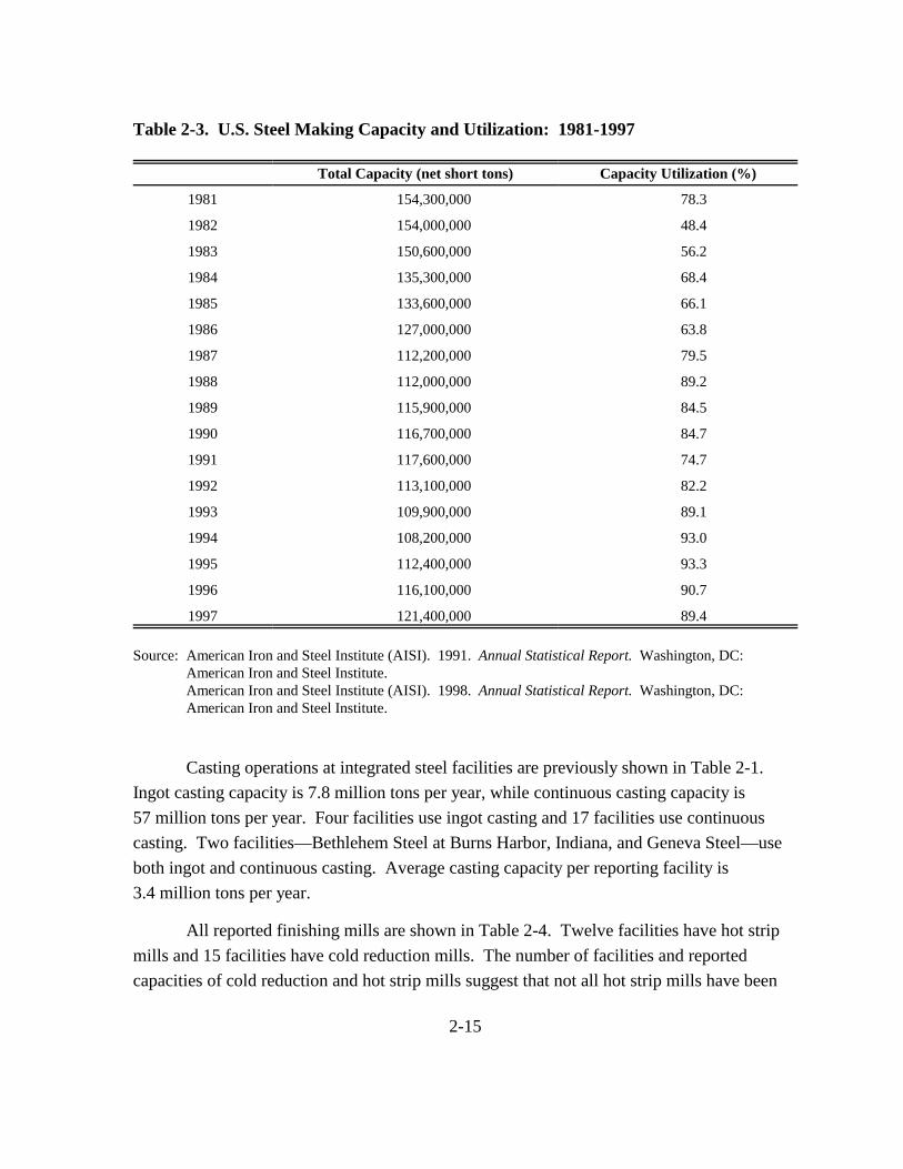
Table 2-3. U.S. Steel Making Capacity and Utilization: 1981-1997

Total Capacity (net short tons) Capacity Utilization (%)

1981 154,300,000 78.3

1982 154,000,000 48.4

1983 150,600,000 56.2

1984 135,300,000 68.4

1985 133,600,000 66.1

1986 127,000,000 63.8

1987 112,200,000 79.5

1988 112,000,000 89.2

1989 115,900,000 84.5

1990 116,700,000 84.7

1991 117,600,000 74.7

1992 113,100,000 82.2

1993 109,900,000 89.1

1994 108,200,000 93.0

1995 112,400,000 93.3

1996 116,100,000 90.7

1997 121,400,000 89.4

Source: American Iron and Steel Institute (AISI). 1991. Annual Statistical Report. Washington, DC: American Iron and Steel Institute. American Iron and Steel Institute (AISI). 1998. Annual Statistical Report. Washington, DC: American Iron and Steel Institute.

Casting operations at integrated steel facilities are previously shown in Table 2-1. Ingot casting capacity is 7.8 million tons per year, while continuous casting capacity is 57 million tons per year. Four facilities use ingot casting and 17 facilities use continuous casting. Two facilities—Bethlehem Steel at Burns Harbor, Indiana, and Geneva Steel—use both ingot and continuous casting. Average casting capacity per reporting facility is 3.4 million tons per year.

All reported finishing mills are shown in Table 2-4. Twelve facilities have hot strip mills and 15 facilities have cold reduction mills. The number of facilities and reported capacities of cold reduction and hot strip mills suggest that not all hot strip mills have been

2-15

900,

000

NA

(con

tinue

d)

Col

d R

educ

tion

Mill

s

1,75

0,00

0

5,30

0,00

0

3,00

0,00

0

5,20

0,00

0

5,80

0,00

0

4,20

0,00

0

3,00

0,00

0

3,43

0,00

0

3,50

0,00

0

1,90

0,00

0

6,10

0,00

0

Cap

acity

Num

ber

Tab

le 2

-4.

Sum

mar

y of

Fin

ishi

ng M

ills a

t Int

egra

ted

Iron

and

Ste

el F

acili

ties:

199

7 (s

hort

tons

per

yea

r)

NA

2 0 1 1 2 1 0 2 1 1 1 1 1 1 0 0

Cap

acity

340,

000 0

3,00

0,00

0

1,58

0,00

0 0 0 0

2,41

0,00

0

2,18

0,00

0

777,

000

2,70

0,00

0

1,80

0,00

0

1,60

0,00

0

3,56

5,00

0 0 0

Hot

Str

ip M

ills

NA

Num

ber

NA

2 0 1 2 0 1 0 2 2 1 2 1 1 3 0 0

Cap

acity

0 0 0

600,

000 0

500,

000 0 0 0 0 0 0 0 0 0 0

NA

Plat

e M

ills

Num

ber

NA

0 0 0 1 0 1 0 0 0 0 0 0 0 0 0 0

Cap

acity

0 0 0 0 0 0 0 0 0 0 0 0

690,

000 0 0 0

Pipe

/Tub

e M

ills

NA

Num

ber

NA

0 0 0 0 0 0 0 0 0 0 0 0 1 0 0 0

Cap

acity

NA

0 0 0 0 0 0 0 0 0 0 0 0 0 0 0 0

Rod

Mill

s

Num

ber

NA

0 0 0 0 0 0 0 0 0 0 0 0 0 0 0 0

Cap

acity

NA

0 0 0 0 0 0 0 0 0 0 0 0 0 0 0 0

Wir

e M

ills

Num

ber

NA

0 0 0 0 0 0 0 0 0 0 0 0 0 0 0 0

Bar

Mill

s

Loca

tion

Cap

acity

0 0 0 0 0 0

1,30

0,00

0 0 0 0 0 0 0 0 0 0

NA

Num

ber

NA

0 0 0 O

H

0 Pt

., M

D

0 0 2 C

hica

go, I

N

0 O

H

0 C

hica

go, I

N

0 IL

0 0 M

I

0 0 0 H

arbo

r, IN

0 PA

Gad

sden

, AL

Stee

l

Riv

erda

le, I

L C

ompa

ny

Ash

land

, KY

Fairf

ield

, AL

Gra

nite

City

, St

eel

Mid

dlet

own,

Lora

in, O

H

Stee

l

Ecor

se, M

I St

eel

Cle

vela

nd,

Bra

ddoc

k,

Ore

m, U

T St

eel

Dea

rbor

n,

Stee

l

Spar

row

s St

eel

Gar

y, IN

Bur

ns

Stee

l

East

East

St

eel

Acm

e St

eel

Gul

f Sta

tes

Bet

hleh

em

Bet

hleh

em

USS

/Kob

e

LTV

Ste

el

LTV

Ste

el

Faci

lity

Nam

e

AK

Ste

el

AK

Ste

el

Nat

iona

l

Nat

iona

l

Gen

eva

Rou

ge

Inla

nd

USX

USX

USX

2-16

0 0 0 0

Col

d R

educ

tion

Mill

s

1,50

0,00

0

3,80

0,00

0

2,85

0,00

0

52,2

30,0

00

Cap

acity

Num

ber

1 1 1 1823

,872

,000

Cap

acity

576,

000

3,34

4,00

0 0

Hot

Str

ip M

ills

Tab

le 2

-4.

Sum

mar

y of

Fin

ishi

ng M

ills a

t Int

egra

ted

Iron

and

Ste

el F

acili

ties:

199

7 (C

ontin

ued)

(s

hort

tons

per

yea

r)

Num

ber

1 5 0 24

Cap

acity

0 0 0

1,10

0,00

0

Plat

e M

ills

Num

ber

0 0 0 2

Pitts

burg

h, P

A:

AIS

E.

Cap

acity

0 0 0

690,

000

Pipe

/Tub

e M

ills

Num

ber

0 0 0 1

1998

. 19

98 D

irect

ory

Iron

and

Ste

el P

lant

s.

Cap

acity

0 0 0 0

Rod

Mill

s

Num

ber

0 0 0 0

Cap

acity

0 0 0 0

Wir

e M

ills

Num

ber

0 0 0 0

Sour

ces:

Ass

ocia

tion

of Ir

on a

nd S

teel

Eng

inee

rs (A

ISE)

.

Bar

Mill

s

Loca

tion

Cap

acity

0 0 0

1,30

0,00

0

Num

ber

0W

arre

n, O

H

0 W

V

0 Ju

nctio

n, O

H

2

Wei

rton,

St

eel

Min

go

Pitts

burg

h

NA

= n

ot a

vaila

ble.

Whe

elin

g-

WC

I Ste

el

Faci

lity

Nam

e

Wei

rton

Tota

l

2-17

reported, considering that steel must go through a hot strip mill before it can go through a cold reduction mill. In addition, only two bar mills, two plate mills, and one pipe/tube mill are shown, reflecting either a lack of reporting, or that the integrated producers conduct a large amount of their finishing operations at other facilities. Integrated iron and steel industry summary data for 1997 are shown in Table 2-5.

2.2.2 Companies

Companies that own individual facilities are legal business entities that have the capacity to conduct business transactions and make business decisions that affect the facility. This section presents information on the parent companies that own the integrated iron and steel facilities identified in Section 2.2.1.

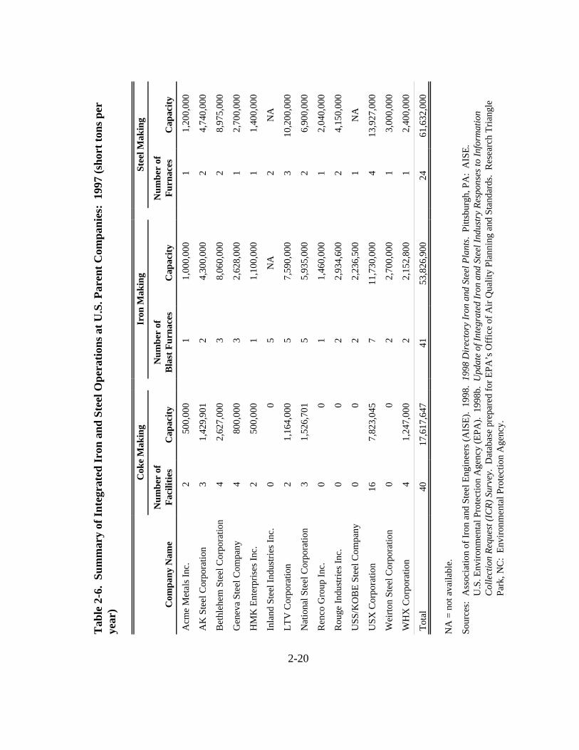
As shown in Table 2-6, 14 companies own the integrated iron and steel facilities identified in Section 2.2.1. USX Corporation has the most production capacity for coke making, iron making, and steel making, while Acme Metals Inc. has the least capacity of all companies owning integrated facilities.

Total annual sales for these companies are presented in Table 2-7. Sales for integrated producers range from $335 million to $6.5 billion, with an average of $3.5 billion. Company-level employment ranges from 2,471 to 41,620 employees and averages 9,536 employees. According to the Small Business Administration’s (SBA’s) criterion (e.g., fewer than 1,000 employees), none of the companies owning integrated iron and steel facilities are classified as small businesses.

Ten companies are publicly traded. HMK Enterprises, Inc., which owns Gulf States Steel, and WHX Corporation, which owns Wheeling-Pittsburgh Steel, are both private companies. National Steel is a subsidiary of NKK USA, a Japanese company. USS/Kobe Steel Company is a joint venture of U.S. Steel Corporation and Kobe Steel, a Japanese public company.

Many of the companies that own integrated mills own multiple facilities, indicating horizontal integration. Some companies also have additional vertical integration. Companies may own service centers to distribute their steel products, or coal and iron ore mines and transportation operations to capture the early stages of steel production. For example, Bethlehem Steel owns BethForge, which manufactures forged steel and cast iron products, and BethShip, which services ships and fabricates some industrial products.

2-18

Table 2-5. Integrated Iron and Steel Industry Summary Data: 1997a

Coke Making

Total coke batteries (#)

Average number per facility

Total coke capacity (short tons/year)

Average capacity per facility

Iron Making

Total number of blast furnaces (#)

Average number per facility

Total blast furnace capacity (short tons/year)

Average capacity per facility

Steel Making

Total number of furnaces (#)

Average number per facility

Total furnace capacity (short tons/year)

Average capacity per facility

Casting

Total casting capacity (short tons/year)

Average capacity per facility

Finishing

Total number of finishing mills (#)

Average number per facility

Total capacity of finishing mills (short tons/year)

Average capacity per facility

38

2.92

15,270,129

1,174,625

41

2.05

53,826,900

2,691,345

24

1.20

61,632,000

3,081,600

64,840,000

3,242,000

47

2.35

79,192,000

3,959,600

a Excludes facilities without capacity information from EPA survey.

Sources: Association of Iron and Steel Engineers (AISE). 1998. 1998 Directory Iron and Steel Plants. Pittsburgh, PA: AISE. U.S. Environmental Protection Agency (EPA). 1998b. Update of Integrated Iron and Steel Industry Responses to Information Collection Request (ICR) Survey. Database prepared for EPA’s Office of Air Quality Planning and Standards. Research Triangle Park, NC: Environmental Protection Agency.

2-19

Tab

le 2

-6.

Sum

mar

y of

Inte

grat

ed Ir

on a

nd S

teel

Ope

ratio

ns a

t U.S

. Par

ent C

ompa

nies

: 19

97 (s

hort

tons

per

ye

ar)

Cok

e M

akin

g Ir

on M

akin

g St

eel M

akin

g

Num

ber

of

Num

ber

of

Num

ber

of

Com

pany

Nam

e Fa

cilit

ies

Cap

acity

Bl

ast F

urna

ces

Cap

acity

Fu

rnac

es

Cap

acity

Acm

e M

etal

s Inc

. 2

500,

000

1 1,

000,

000

1 1,

200,

000

AK

Ste

el C

orpo

ratio

n 3

1,42

9,90

1 2

4,30

0,00

0 2

4,74

0,00

0

Bet

hleh

em S

teel

Cor

pora

tion

4 2,

627,

000

3 8,

060,

000

2 8,

975,

000

Gen

eva

Stee

l Com

pany

4

800,

000

3 2,

628,

000

1 2,

700,

000

HM

K E

nter

pris

es In

c.

2 50

0,00

0 1

1,10

0,00

0 1

1,40

0,00

0

Inla

nd S

teel

Indu

strie

s Inc

. 0

0 5

NA

2

NA

LTV

Cor

pora

tion

2 1,

164,

000

5 7,

590,

000

3 10

,200

,000

Nat

iona

l Ste

el C

orpo

ratio

n 3

1,52

6,70

1 5

5,93

5,00

0 2

6,90

0,00

0

Ren

co G

roup

Inc.

0

0 1

1,46

0,00

0 1

2,04

0,00

0

Rou

ge In

dust

ries I

nc.

0 0

2 2,

934,

600

2 4,

150,

000

USS

/KO

BE

Stee

l Com

pany

0

0 2

2,2

36,5

00

1 N

A

USX

Cor

pora

tion

16

7,82

3,04

5 7

11,7

30,0

00

4 13

,927

,000

Wei

rton

Stee

l Cor

pora

tion

0 0

2 2,

700,

000

1 3,

000,

000

WH

X C

orpo

ratio

n 4

1,24

7,00

0 2

2,15

2,80

0 1

2,40

0,00

0

Tota

l 40

17

,617

,647

41

53

,826

,900

24

61

,632

,000

NA

= n

ot a

vaila

ble.

Sour

ces:

A

ssoc

iatio

n of

Iron

and

Ste

el E

ngin

eers

(AIS

E).

1998

. 19

98 D

irec

tory

Iron

and

Ste

el P

lant

s. Pi

ttsbu

rgh,

PA

: A

ISE.

U

.S. E

nviro

nmen

tal P

rote

ctio

n A

genc

y (E

PA).

1998

b. U

pdat

e of

Inte

grat

ed Ir

on a

nd S

teel

Indu

stry

Res

pons

es to

Info

rmat

ion

Col

lect

ion

Requ

est (

ICR)

Sur

vey.

Dat

abas

e pr

epar

ed fo

r EPA

’s O

ffic

e of

Air

Qua

lity

Plan

ning

and

Sta

ndar

ds.

Res

earc

h Tr

iang

le

Park

, NC

: En

viro

nmen

tal P

rote

ctio

n A

genc

y.

2-20

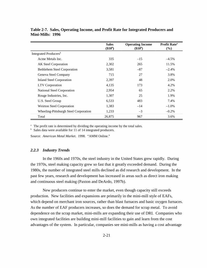
Table 2-7. Sales, Operating Income, and Profit Rate for Integrated Producers and Mini-Mills: 1996

Sales Operating Income Profit Ratea

($106) ($106) (%) Integrated Producersb

Acme Metals Inc. 335 –15 –4.5% AK Steel Corporation 2,302 265 11.5% Bethlehem Steel Corporation 3,581 –87 –2.4% Geneva Steel Company 715 27 3.8% Inland Steel Corporation 2,397 48 2.0% LTV Corporation 4,135 173 4.2% National Steel Corporation 2,954 65 2.2% Rouge Industries, Inc. 1,307 25 1.9% U.S. Steel Group 6,533 483 7.4% Weirton Steel Corporation 1,383 –14 –1.0% Wheeling-Pittsburgh Steel Corporation 1,233 –3 –0.2% Total 26,875 967 3.6%

a The profit rate is determined by dividing the operating income by the total sales. b Sales data were available for 11 of 14 integrated producers.

Source: American Metal Market. 1998. “AMM Online.”

2.2.3 Industry Trends

In the 1960s and 1970s, the steel industry in the United States grew rapidly. During the 1970s, steel making capacity grew so fast that it greatly exceeded demand. During the 1980s, the number of integrated steel mills declined as did research and development. In the past few years, research and development has increased in areas such as direct iron making and continuous steel making (Paxton and DeArdo, 1997b).

New producers continue to enter the market, even though capacity still exceeds production. New facilities and expansions are primarily in the mini-mill style of EAFs, which depend on merchant iron sources, rather than blast furnaces and basic oxygen furnaces. As the number of EAF producers increases, so does the demand for scrap metal. To avoid dependence on the scrap market, mini-mills are expanding their use of DRI. Companies who own integrated facilities are building mini-mill facilities to gain and learn from the cost advantages of the system. In particular, companies see mini-mills as having a cost advantage

2-21

for flat rolled sheet metal (Samways, 1998). For example, Trico Steel is a mini-mill that was formed as a joint venture by three companies owning integrated steel mills, the only U.S. company being LTV. Mini-mills are increasingly targeting high end markets for steel products, such as the automobile industry. Some experts in the steel industry believe that integrated mills may be forced to sell pig iron to mini-mills and sell cold rolled and coated steel themselves (Berry, 1997). National Steel, Weirton Steel, AK Steel, and Bethlehem Steel may be following this advice because they have all increased their cold rolled line capacity in 1998 (Woker, 1998).

Integrated mills and their parent companies are also expanding overseas. As automakers expand their operations abroad, they are encouraging U.S. steel makers who they are currently dealing with to expand operations overseas or to merge with foreign producers (Ritt, 1998).

2.3 Uses and Consumers

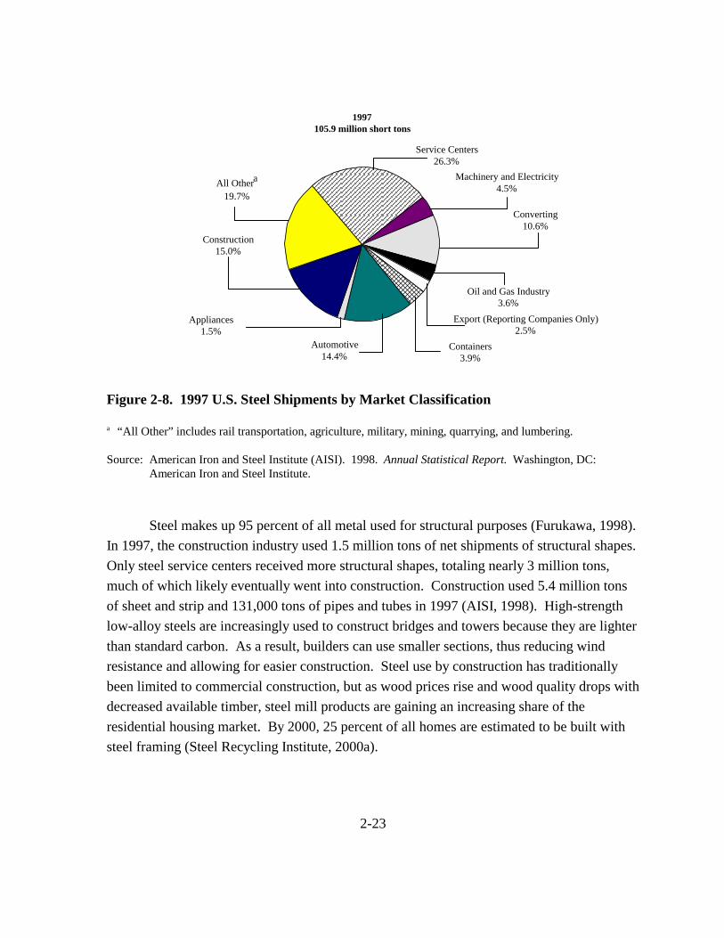
Construction and automotive industries are the two largest demanders of finished steel products, consuming 15 percent and 14.4 percent, respectively, of total net shipments in 1997. Although service centers are the single largest market group represented in Figure 2-8, they are not a single end user group because they represent businesses that buy steel mill products at wholesale and then resell them. Steel for converting is also not separated into a specific end-user group.

Over 90 percent of structural components by weight in automobiles are iron-based (Paxton and DeArdo, 1997b). In 1997, the automotive industry used 12.6 million tons of sheet and strip (AISI, 1998). The automotive industry also used 1.4 million tons of bars in 1997. Steel mill products are used for large automobile parts, such as body panels. One technique by steel makers is the use of high strength steel to address the automobile industry’s need for lighter vehicles to achieve fuel efficiency gains. High strength steels are harder than the alloy steels traditionally used in the industry, meaning that less mass is necessary to build the same size vehicle. An UltraLight Steel Auto Body has recently been designed that has a 36 percent decrease in mass from a standard frame (Steel Alliance, 1998). Drawbacks are that the harder steels require additional processing to achieve a thin gauge, and manufacturing with high strength steels demands more care and effort due to the low levels of ductility (Autosteel, 1998a).

2-22

1997105.9 million short tons

Service Centers

1.5%

3.9%

26.3% Machinery and Electricity

4.5%

Converting 10.6%

Oil and Gas Industry 3.6%

Export (Reporting Companies Only) 2.5%

Containers Automotive 14.4%

Appliances

Construction 15.0%

All Othera

19.7%

Figure 2-8. 1997 U.S. Steel Shipments by Market Classification

a “All Other” includes rail transportation, agriculture, military, mining, quarrying, and lumbering.

Source: American Iron and Steel Institute (AISI). 1998. Annual Statistical Report. Washington, DC: American Iron and Steel Institute.

Steel makes up 95 percent of all metal used for structural purposes (Furukawa, 1998). In 1997, the construction industry used 1.5 million tons of net shipments of structural shapes. Only steel service centers received more structural shapes, totaling nearly 3 million tons, much of which likely eventually went into construction. Construction used 5.4 million tons of sheet and strip and 131,000 tons of pipes and tubes in 1997 (AISI, 1998). High-strength low-alloy steels are increasingly used to construct bridges and towers because they are lighter than standard carbon. As a result, builders can use smaller sections, thus reducing wind resistance and allowing for easier construction. Steel use by construction has traditionally been limited to commercial construction, but as wood prices rise and wood quality drops with decreased available timber, steel mill products are gaining an increasing share of the residential housing market. By 2000, 25 percent of all homes are estimated to be built with steel framing (Steel Recycling Institute, 2000a).

2-23

Seventy-five percent of the weight of the average appliance is due to steel (Steel Recycling Institute, 2000b). Appliances, including utensils and cutlery, were responsible for 1.6 million tons of net shipments of steel mill products in 1997. The appliance market also received bars, pipes, tin mill products, and wire rods (AISI, 1998).

About 95 percent of all food cans in North America are made out of steel; per capita use of steel cans in North America is 120 cans (AISI, 1998). In 1997, the container industry received 3.2 million tons of tin mill products, or 79 percent of all tin mill product net shipments in 1997 (AISI, 1998). In addition, 870,000 tons of sheet and strip were shipped to the container industry in 1997.

Because steel is used for such diverse products, there are numerous possible substitutes for it. In Table 2-8, alloy and carbon steel are compared to some possible substitutes. The density of both steels is greater than any of the substitutes, leading to greater weight. The cost per ton of all substitute materials is much higher than steel, except for wood and reinforced concrete. In addition, total annual production of the top three possible replacements (aluminum, magnesium, and titanium) is only 4 million tons, less than 5 percent of steel’s annual production. Thus, the threat of major replacement by substitutes is low (Paxton and DeArdo, 1997a).

2.4 Historic Market Data

2.4.1 Steel Mill Products

Table 2-9 presents historic data for all steel mill products. From 1981 to 1997, U.S. production of steel mill products increased by 1.2 percent; from 1989 to 1997, production increased by 3.2 percent, showing accelerating growth in shipments. Export growth slowed from 1989 to 1997 relative to 1981 to 1989, with average annual growth decreasing from 7.2 percent to 4 percent.

As shown in Table 2-10, import average annual growth rates increased sharply during the period 1991 to 1997, due in part to a large supply of cheap steel from Asia. Many U.S. companies are seeking legislation to prevent foreign companies from dumping steel in the United States at low prices. In February 1999, the U.S. Department of Commerce found that Brazil and Japan have illegally dumped steel in the United States at up to 70 percent below the normal price (Associated Press, 1999).

2-24

Table 2-8. Comparison of Steel and Substitutes by Cost, Strength, and Availability: 1997

Absolute Absolute Yield Production Production

Strength Density Cost $/metric Weight Volume MN/m2 Mg/m3 ton (106 tons/yr) (106 m3/yr)

Reinforced concrete

Wood

Alloy steel

Carbon steel

Aluminum alloy

Magnesium alloy

Titanium alloy

50 2.5 40

70 0.55 400

1,000 7.87 826

220 7.87 385 to 600

1,300 2.7 3,500

140 1.74 3,200

800 4.5 18,750

Glass-fiber reinforced plastic 200 1.8 3,900

Carbon-fiber reinforced plastic 600 1.5 113,000

500

69

86.2 (all steel)

–a

3.8

0.13

0.06

NA

NA

200

125

11 (all steel)

–a

1.4

0.07

0.01

NA

NA

a Production of carbon steel included with alloy steel. NA = not available

Source: Paxton, H.W., and A.J. DeArdo. January 1997a. “Steel vs. Aluminum, Plastic, and the Rest.” New Steel.

U.S. apparent consumption average annual growth rates also increased from –1 percent for 1981 to 1989 to 4.4 percent for 1989 to 1997. The strengthening U.S. economy, with greater consumption, including automobiles and new construction with expanding and new companies, has increased the demand for steel in the United States.

As shown in Table 2-11, the average export concentration ratio has increased from 0.02 for 1981 to 1988 to 0.06 for 1989 to 1997. Increasing export concentration ratios indicate that a greater percentage of U.S. production is being sold overseas. Average import concentration ratios decreased slightly from 0.22 for 1981 to 1988 to 0.20 for 1989 to 1997, suggesting that imports’ share of U.S. consumption has increased only slightly.

2-25

1.2%

3.2%

88,4

50

73,7

39

73,0

43

70,2

63

76,6

54

83,8

40

84,1

00

84,9

81

78,8

46

82,2

41

89,0

22

61,5

67

67,5

84

95,0

84

97,4

94

100,

878

105,

858

–0.6

%

Tot

alA

ll O

ther

a

0.0%

–1

.4%

1.

7%

13,5

35

12,7

07

13,1

79

14,5

99

18,5

51

13,4

49

11,3

66

15,3

28

16,4

09

15,9

80

13,9

84

14,6

97

15,7

22

17,0

23

16,2

69

17,0

76

18,6

51

Tab

le 2

-9.

Net

Shi

pmen

ts o

f Ste

el M

ill P

rodu

cts b

y M

arke

t Cla

ssifi

catio

n: 1

981-

1997

(103 sh

ort t

ons)

Sour

ces:

Am

eric

an Ir

on a

nd S

teel

Inst

itute

(AIS

I).

1991

. An

nual

Sta

tistic

al R

epor

t. W

ashi

ngto

n, D

C:

Am

eric

an Ir

on a

nd S

teel

Inst

itute

. A

mer

ican

Iron

and

Ste

el In

stitu

te (A

ISI)

. 19

93.

Annu

al S

tatis

tical

Rep

ort.

Was

hing

ton,

DC

: A

mer

ican

Iron

and

Ste

el In

stitu

te.

Am

eric

an Ir

on a

nd S

teel

Inst

itute

(AIS

I).

1998

. An

nual

Sta

tistic

al R

epor

t. W

ashi

ngto

n, D

C:

Am

eric

an Ir

on a

nd S

teel

Inst

itute

.

Exp

orts

2.6%

9.

1%

–2.3

%

428

494

495

515

1,84

5 83

2 54

4

1,23

3 3,

183

2,48

7 4,

476

2,65

0 2,

110

1,71

0 4,

442

2,32

8 2,

610

“All

Oth

er”

incl

udes

rail

trans

porta

tion,

airc

raft

and

aero

spac

e, sh

ipbu

ildin

g, m

inin

g, a

gric

ultu

re, a

nd n

oncl

assi

fied

ship

men

ts.

Con

vert

ing

5,13

6 5,

484

5,63

5 7,

195

5,05

8 3,

222

4,40

3

8,79

2 8,

235

9,44

1 8,

265

9,22

6 9,

451

10,5

02

10,4

40

10,2

45

11,2

63

7.7%

4.6%

7.

9%

Cen

ters

18,3

64

18,4

39

17,4

78

19,8

40

17,6

37

13,0

67

16,7

10

21,0

37

20,7

69

21,1

11

19,4

64

21,3

28

23,7

14

24,1

53

23,7

51

27,1

24

27,8

00

Serv

ice

Elec

tric

ity

3.6%

2.

2%

4.2%

Mac

hine

ry a

nd

Gas

–2.1

%

–4.1

%

–0.2

%

7,22

4 4,

587

4,82

1 5,

251

4,14

0 4,

189

4,65

0 5,

257

4,85

8 4,

841

4,08

4 4,

087

4,40

4 4,

726

4,70

7 4,

811

4,78

9 A

vera

ge A

nnua

l Gro

wth

Rat

es

Oil

and

Con

tain

ers

–2.4

%

27.1

%

–10.

1%

6,23

8 2,

745

1,29

6 2,

003

2,04

4 1,

023

1,48

9 1,

477

1,20

3 1,

892

1,42

5 1,

454

1,52

6 1,

703

2,64

3 3,

254

3,81

1

–1.3

%

–2.0

%

–0.8

%

5,29

2 4,

470

4,53

2 4,

352

4,08

9 4,

113

4,37

2 4,

421

4,45

9 4,

474

4,27

8 3,

974

4,35

5 4,

495

4,13

9 4,

101

4,16

3

App

lianc

es

–0.5

%

–0.4

%

–0.6

%

1,77

5 1,

337

1,61

8 1,

635

1,46

6 1,

648

1,63

3 1,

638

1,72

1 1,

540

1,38

8 1,

503

1,59

2 1,

736

1,58

9 1,

713

1,63

5

Con

stru

ctio

n

11,6

76

8,57

0 9,

974

10,1

53

11,2

30

10,6

14

11,0

18

12,1

02

11,5

00

12,1

15

11,4

67

12,2

30

13,4

29

14,2

83

14,8

92

15,5

61

15,8

85

2.3%

4.8%

–0

.2%

Aut

omot

ive

13,1

54

9,28

8 12

,320

12

,882

12

,950

11

,889

11

,343

12

,555

11

,763

11

,100

10

,015

11

,092

12

,719

14

,753

14

,622

14

,665

15

,251

1.0%

–1

.3%

3.

7%

1981

-199

7 19

81-1

989

1989

-199

7

Yea

r

1981

19

82

1983

19

84

1985

19

86

1987

19

88

1989

19

90

1991

19

92

1993

19

94

1995

19

96

1997

a

2-26

Table 2-10. U.S. Production, Foreign Trade, and Apparent Consumption of Steel Mill Products: 1981-1997 (103 short tons)

Apparent Productiona Exports Imports Consumptionb

1981 88,450 2,904 19,898 105,444

1982 61,567 1,842 16,663 76,388

1983 67,584 1,199 17,070 83,455

1984 73,739 980 26,163 98,922

1985 73,043 932 24,256 96,367

1986 70,263 929 20,692 90,026

1987 76,654 1,129 20,414 95,939

1988 83,840 2,069 20,891 102,662

1989 84,100 4,578 17,321 96,843

1990 84,981 4,303 17,169 97,847

1991 78,846 6,346 15,845 88,345

1992 82,241 4,288 17,075 95,028

1993 89,022 3,968 19,501 104,555

1994 95,084 3,826 30,066 121,324

1995 97,494 7,080 24,409 114,823

1996 100,878 5,031 29,164 125,011

1997 105,858 6,036 31,157 130,979

Average Annual Growth Rates

1981-1997 1.2% 6.7% 3.5% 1.5%

1981-1989 –0.6% 7.2% –1.6% –1.0%

1989-1997 3.2% 4.0% 10.0% 4.4%

a Measured as net shipments, which are total production minus intracompany transfers. b Equals U.S. production minus exports plus imports.

Sources: American Iron and Steel Institute (AISI). 1991. Annual Statistical Report. Washington, DC: American Iron and Steel Institute. American Iron and Steel Institute (AISI). 1993. Annual Statistical Report. Washington, DC: American Iron and Steel Institute. American Iron and Steel Institute (AISI). 1998. Annual Statistical Report. Washington, DC: American Iron and Steel Institute.

2-27

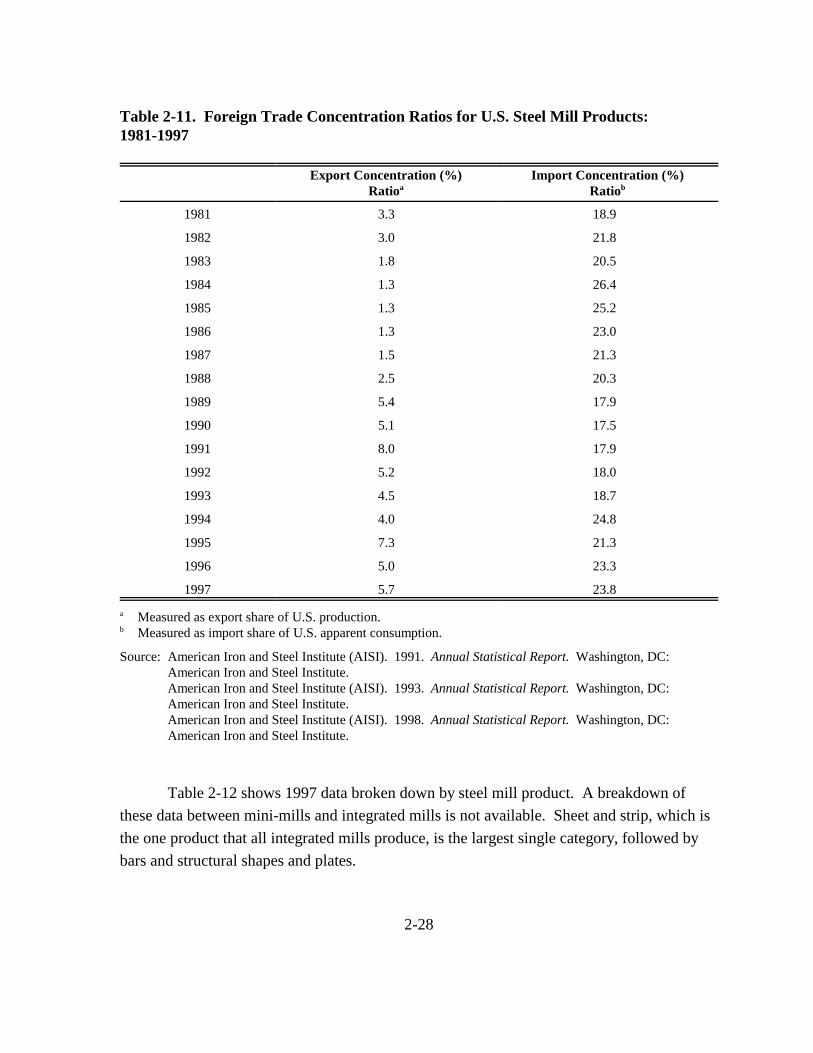
Table 2-11. Foreign Trade Concentration Ratios for U.S. Steel Mill Products: 1981-1997

Export Concentration (%) Import Concentration (%) Ratioa Ratiob

1981 3.3 18.9

1982 3.0 21.8

1983 1.8 20.5

1984 1.3 26.4

1985 1.3 25.2

1986 1.3 23.0

1987 1.5 21.3

1988 2.5 20.3

1989 5.4 17.9

1990 5.1 17.5

1991 8.0 17.9

1992 5.2 18.0

1993 4.5 18.7

1994 4.0 24.8

1995 7.3 21.3

1996 5.0 23.3

1997 5.7 23.8

a Measured as export share of U.S. production. b Measured as import share of U.S. apparent consumption.

Source: American Iron and Steel Institute (AISI). 1991. Annual Statistical Report. Washington, DC: American Iron and Steel Institute. American Iron and Steel Institute (AISI). 1993. Annual Statistical Report. Washington, DC: American Iron and Steel Institute. American Iron and Steel Institute (AISI). 1998. Annual Statistical Report. Washington, DC: American Iron and Steel Institute.

Table 2-12 shows 1997 data broken down by steel mill product. A breakdown of these data between mini-mills and integrated mills is not available. Sheet and strip, which is the one product that all integrated mills produce, is the largest single category, followed by bars and structural shapes and plates.

2-28

Table 2-12. U.S. Production, Foreign Trade, and Apparent Consumption of Steel Mill Products: 1997 (tons)

Apparent Product Productiona Exports Imports Consumptionb

Semi-finished

Structural Shapes and Plate

Rail and Track

Bars

Tool Steel

Pipe and Tube

Wire-drawn

Tin Mill

Sheet and Strip

7,927,145 295,325 8,595,964 16,227,784

14,883,805 1,260,197 4,079,451 17,703,059

874,648 92,095 238,190 1,020,743

18,708,680 820,523 2,495,817 20,383,974

63,465 14,745 131,363 180,083

6,547,953 1,352,006 3,030,239 8,226,186

619,070 136,697 655,000 1,137,373

4,058,054 410,011 637,000 4,285,043

52,175,194 1,653,990 11,293,000 61,814,204

a Reflects net shipments, which are total shipments minus intracompany transfers. b Reflects U.S. production minus exports, plus imports.

Source: American Iron and Steel Institute (AISI). 1998. Annual Statistical Report. Washington, DC: American Iron and Steel Institute.

In general, production and consumption of steel mill products have increased over the last 10 years, suggesting that the steel market is strengthening. The health of the steel industry is closely tied to the health of the United States and world economy, because steel is a major component of a wide variety of products, particularly construction. Imports and exports have also risen, showing opening trade markets and integration of the global economy. Imports did not rise more than exports for a large number of steel mill products, suggesting that the U.S. steel industry is maintaining its foothold in the U.S. steel market.

2.4.2 Market Prices

Table 2-13 shows the prices by steel type for all steel mill products in 1997. Some products are only available in a single type of steel. For example, rails and accessories are only made with carbon steel, tool steel is always alloy steel, and tin mill products always have carbon steel as the base steel. Prices for semi-finished carbon steel are lower than for any other steel mill products, as expected. Wire-drawn steel has the highest carbon steel

2-29

price, at more than twice the price of semi-finished carbon steel. Alloy steel versions of the products are generally more expensive than carbon steel versions with the exception of sheet and strip. This may reflect the more extensive processing and finishing of carbon sheet and strip, such as coatings and treatments. Wire-drawn alloy steel is nearly three times the price of the carbon steel version. Tool steel is the most expensive alloy steel product at more than seven times the price of alloy sheet and strip. The high price of tool steel reflects its highly specialized nature and the fact that alloy mixtures for tool steel have higher raw material costs than other alloy steels.

Stainless steel versions of products are the most expensive for all product types that are available in stainless steel, at several times the price of carbon versions and at least twice the price of alloy versions. High stainless steel prices do not strongly affect average steel mill product prices overall, however, because stainless steel products are typically a small percentage of all steel products of that type.

2.5 Future Projections

2.5.1 Iron Making

Table 2-14 shows projected blast furnace activity through the year 2004. Business Communications Company (BCC) projects that coke consumption will steadily decrease as a result of projected improvements in efficiency. BCC’s projections also reflect anticipated moves to cokeless iron making technologies such as DRI (which is being marketed in the United States by Midrex) and gradual decreases in the use of blast furnaces to provide the iron source for steel making.

2.5.2 Steel Making and Casting

Table 2-15 shows projected apparent consumption of steel mill products. BCC expects overall U.S. steel production to increase until 2004. Largely powered by the success of the mini-mills, EAFs are expected to produce increasing amounts of steel, and their share of total steel production is also projected to rise. Basic oxygen furnaces and EAFs are both expected to increase their consumption of scrap metal as an iron source, and basic oxygen furnaces are also expected to decrease their consumption of pig iron. Pig iron production as a whole will likely decrease, but integrated mills are expected to sell more pig iron to mini-mills than they currently do, as a result of the increasing pig iron content of electric arc furnace charge. Basic oxygen furnaces and EAFs are both expected to increase their

2-30

Table 2-13. Market Prices and Net Shipments of Steel Mill Products by Steel Type: 1997

Type of Steel

Product Carbon Alloy Stainless All Types

Pricea ($/short ton)

Semi-finished

Structural shapes and plates

Rails and accessories

Bars

Tool steel

Pipe and tubing

Wire-drawn

Tin mill

Sheet and strip

$371.57 $984.35 $1,368.45 $494.58

435.68 634.09 2,708.48 496.19

639.90 NA NA 639.90

436.76 669.65 4,083.75 508.52

NA 4,682.22 NA 4,682.22

714.63 1,003.14 4,290.63 805.88

847.24 2,273.81 4,937.19 922.42

594.60 NA NA 594.60

639.60 599.21 2,134.45 677.92

All steel mill products 581.35 792.39 2,405.67 639.74

Net Shipments (short tons)

Semi-finished

Structural shapes and plates

Rails and accessories

Bars

Tool steel

Pipe and tubing

Wire-drawn

Tin mill

Sheet and strip

6,887,123 961,504 78,518 7,927,145

14,186,751 437,048 260,006 14,883,805

874,648 NA NA 874,648

16,082,256 2,454,364 172,060 18,708,680

NA 63,465 NA 63,465

5,278,694 1,236,073 33,186 6,547,953

564,891 28,614 25,565 619,070

4,058,054 NA NA 4,058,054

49,576,735 1,100,830 1,497,629 52,175,194

All steel mill products 97,509,152 6,281,898 2,066,964 105,858,014

a Price calculated by dividing value of shipments by quantity of shipments. NA = Not available because product is not made with this type of steel.

Sources: American Iron and Steel Institute (AISI). 1998. Annual Statistical Report. Washington, DC: American Iron and Steel Institute. U.S. Department of Commerce. 1997. Current Industrial Reports. Washington, DC: Bureau of the Census.

2-31

Table 2-14. Projected U.S. Production, Foreign Trade, and Apparent Consumption of Steel Mill Products: 1994, 1999, and 2004 (103 short tons)

Apparent Year Productiona Exports Imports Consumptionb

1994 97,372 5,902 30,130 121,600

1999 104,000 7,000 23,000 120,000

2004 107,000 5,500 24,500 126,000

Average Annual Growth Rates

1994-2004 1.0% –0.7% –1.9% 0.4%

1994-1999 1.4% 3.7% –4.7% –0.3%

1999-2004 0.6% –4.3% 1.3% 1.0%

a Measures as net shipments, which are total production minus intracompany transfers. b Equals U.S. production minus exports plus imports.

Source: Business Communications Company. October 1995. “The Future of the Steel Industry in the U.S.”

Table 2-15. Projected U.S. Apparent Consumption of Steel Mill Product by Type: 1994, 1999, and 2004 (103 short tons)

Structural Shapes and Pipes and Sheet and

Year Plates Bars Tubing Strip All Others Total

1994 16,300 18,000 7,200 57,200 22,900 121,600

1999 15,950 17,800 7,240 56,870 22,140 120,000

2004 17,550 19,500 7,300 58,000 23,650 126,000

Average Annual Growth Rates

1994-2004 0.8% 0.8% 0.1% 0.1% 0.3% 0.4%

1994-1999 –0.4% –0.2% 0.1% –0.1% –0.7% –0.3%

1999-2004 2.0% 1.9% 0.2% 0.4% 1.4% 1.0%

Source: Business Communications Company. October 1995. “The Future of the Steel Industry in the U.S.”

2-32

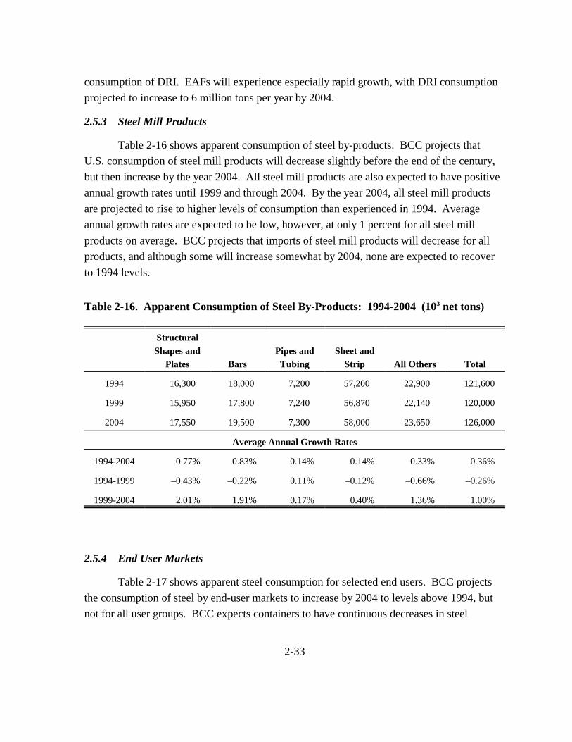
consumption of DRI. EAFs will experience especially rapid growth, with DRI consumption projected to increase to 6 million tons per year by 2004.

2.5.3 Steel Mill Products

Table 2-16 shows apparent consumption of steel by-products. BCC projects that U.S. consumption of steel mill products will decrease slightly before the end of the century, but then increase by the year 2004. All steel mill products are also expected to have positive annual growth rates until 1999 and through 2004. By the year 2004, all steel mill products are projected to rise to higher levels of consumption than experienced in 1994. Average annual growth rates are expected to be low, however, at only 1 percent for all steel mill products on average. BCC projects that imports of steel mill products will decrease for all products, and although some will increase somewhat by 2004, none are expected to recover to 1994 levels.

Table 2-16. Apparent Consumption of Steel By-Products: 1994-2004 (103 net tons)

Structural Shapes and Pipes and Sheet and

Plates Bars Tubing Strip All Others Total

1994 16,300 18,000 7,200 57,200 22,900 121,600

1999 15,950 17,800 7,240 56,870 22,140 120,000

2004 17,550 19,500 7,300 58,000 23,650 126,000

Average Annual Growth Rates

1994-2004 0.77% 0.83% 0.14% 0.14% 0.33% 0.36%

1994-1999 –0.43% –0.22% 0.11% –0.12% –0.66% –0.26%

1999-2004 2.01% 1.91% 0.17% 0.40% 1.36% 1.00%

2.5.4 End User Markets

Table 2-17 shows apparent steel consumption for selected end users. BCC projects the consumption of steel by end-user markets to increase by 2004 to levels above 1994, but not for all user groups. BCC expects containers to have continuous decreases in steel

2-33

Tab

le 2

-17.

App

aren

t Ste

el C

onsu

mpt

ion

for

Sele

cted

End

Use

rs:

1994

-200

4 (1

03 net

tons

)

Mac

hine

ry

App

lianc

es,

and

Elec

tric

al

Ute

nsils

, and

A

ll C

onst

ruct

ion

Aut

omot

ive

Oil

and

Gas

E

quip

men

t E

quip

men

t C

utle

ry

Con

tain

ers

Oth

ers

Tota

l

1994

27

,500

26

,500

4,

200

6,00

0 6,

500

4,00

0 6,

600

40,3

00

121,

600

1999

27

,620

24

,830

3,

825

6,00

0 6,

500

4,00

0 6,

400

40,8

25

120,

000

2004

31

,000

26

,000

3,

900

6,15

0 6,

700

4,15

0 6,

225

41,2

75

125,

400

Ave

rage

Ann

ual G

row

th R

ates

1994

-200

4 1.

3%

–0.2

%

–0.7

%

0.3%

0.

3%

0.4%

–0

.6%

0.

2%

0.3%

1994

-199

9 0.

1%

–1.3

%

–1.8

%

0.0%

0.

0%

0.0%

–0

.6%

0.

3%

–0.3

%

1999

-200

4 2.

5%

0.9%

0.

4%

0.5%

0.

6%

0.8%

–0

.6%

0.

2%

0.9%

Sour

ce:

Bus

ines

s Com

mun

icat

ions

Com

pany

. O

ctob

er 1

995.

“Th

e Fu

ture

of t

he S

teel

Indu

stry

in th

e U

.S.”

2-34

consumption, and they project that automotive and oil and gas consumption will not recover to 1994 levels as of 2004. Actual changes in steel consumption levels are quite low, with average annual growth rates between –1 and 1 percent for all groups except construction, automotive, and oil and gas. BCC expects construction to experience increased consumption after 1999, with average annual growth rates of 2.45 percent until 2004. BCC projects that automotive and oil and gas will have negative annual growth greater than –1 percent until 1999.

Table 2-18 shows steel imports by end-use markets. Import patterns for end-user groups are similar to consumption patterns, although more extreme. BCC expects imports by the automotive industry to experience significant decreases until 2004, with an average annual growth rate from 1994 to 1999 of –11 percent.

Decreased steel imports by the automotive industry and decreased overall consumption are due to decreased steel content in automobiles. Steel content has decreased since 1972 (see Section 3), and experts expect the pattern to continue at least until 2000. As shown in Table 2-19, the use of steel by the industry is projected to decrease even more rapidly between 1996 and 2000. BCC projects the automobile industry to have increased demand of aluminum, magnesium, plastics, and glass through the year 2000. BCC expects demand for aluminum to nearly double and demand for magnesium to nearly triple. Despite decreased steel demand and increased demand for other materials, BCC projects the demand for all four other materials to be just over half of the demand for steel.

2-35

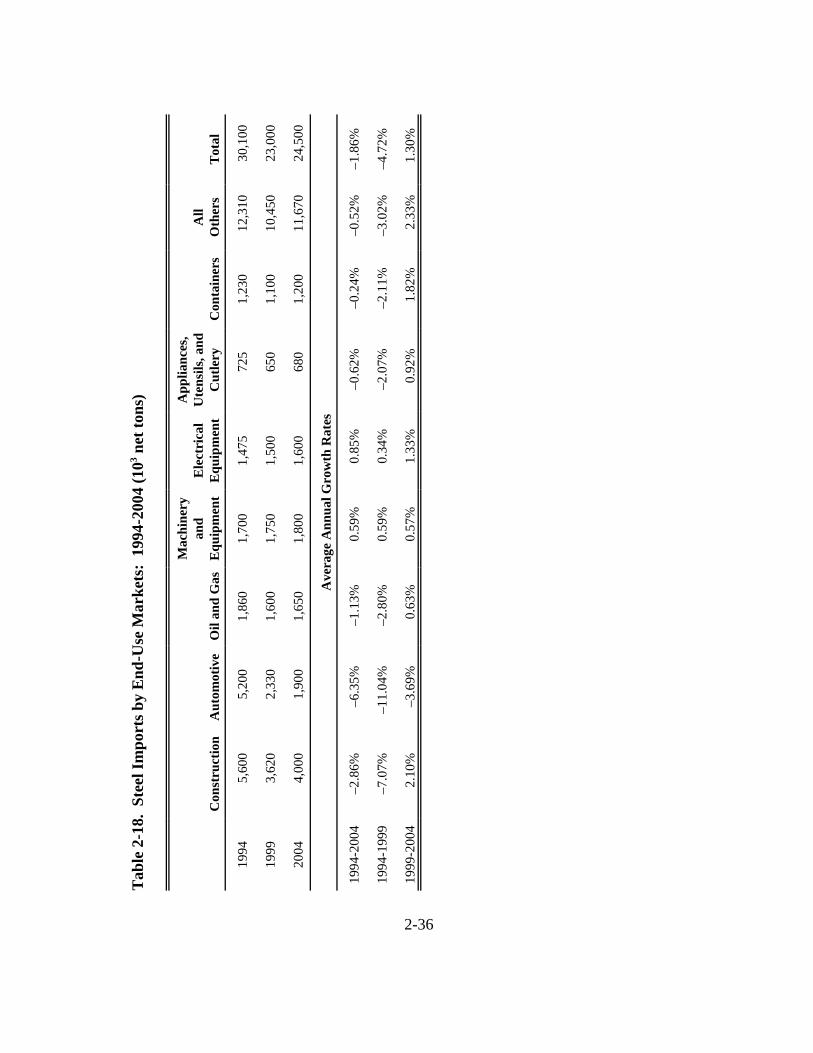
Tab

le 2

-18.

Ste

el Im

port

s by

End

-Use

Mar

kets

: 19

94-2

004

(103 n

et to

ns)

Mac

hine

ry

App

lianc

es,

and

Elec

tric

al

Ute

nsils

, and

A

ll C

onst

ruct

ion

Aut

omot

ive

Oil

and

Gas

E

quip

men

t E

quip

men

t C

utle

ry

Con

tain

ers

Oth

ers

Tota

l

1994

5,

600

5,20

0 1,

860

1,70

0 1,

475

725

1,23

0 12

,310

30

,100

1999

3,

620

2,33

0 1,

600

1,75

0 1,

500

650

1,10

0 10

,450

23

,000

2004

4,

000

1,90

0 1,

650

1,80

0 1,

600

680

1,20

0 11

,670

24

,500

Ave

rage

Ann

ual G

row

th R

ates

1994

-200

4 –2

.86%

–6

.35%

–1

.13%

0.

59%

0.

85%

–0

.62%

–0

.24%

–0

.52%

–1

.86%

1994

-199

9 –7

.07%

–1

1.04

%

–2.8

0%

0.59

%

0.34

%

–2.0

7%

–2.1

1%

–3.0

2%

–4.7

2%

1999

-200

4 2.

10%

–3

.69%

0.

63%

0.

57%

1.

33%

0.

92%

1.

82%

2.

33%

1.

30%

2-36

Table 2-19. Demand Forecast for Raw Materials in Motor Vehicles: 1992, 1996, and 2000 (metric tons)

Steel Aluminum Magnesium Plastics Glass

1992 30 3.2 0.35 5.00 1.00

1996 29 4.1 0.5 5.45 1.05

2000 24 6.0 1.0 6.35 1.08

Average Annual Growth Rates

1992-2000 –2.50% 10.94% 23.21% 3.38% 1.00%

1992-1996 –0.83% 7.03% 10.71% 2.25% 1.25%

1996-2000 –4.31% 11.59% 25.00% 4.13% 0.71%

Source: EIU. “The Material Revolution to the Motor Industry.” September 1993. The Dialog Corporation. <http://www.profound.com>.

2-37

SECTION 3

ENGINEERING COST ANALYSIS

Control measures implemented to comply with the MACT standard will impose regulatory costs on integrated iron and steel mills. This section presents compliance costs for affected mills, or plants, and the national estimate of compliance costs associated with the proposed rule. These engineering costs are defined as the annual capital and operating and maintenance costs assuming no behavioral market adjustment by producers or consumers. For input to the EIA, engineering costs are expressed per unit of steel mill product and used to shift the individual mill supply functions in the market model.

The proposed MACT will cover the Integrated Iron and Steel Manufacturing source category. As such it will affect 20 integrated iron and steel mills across the nation. The processes covered by the proposed regulation include sinter production, iron production in blast furnaces, and basic oxygen process furnace (BOPF) shops, which includes hot metal transfer, slag skimming, steelmaking in BOPFs, and ladle metallurgy. Capital, operating and maintenance, and monitoring costs were estimated for each plant, where appropriate. All 20 plants will be required to install additional monitoring equipment, while new or upgraded control equipment will be required at four of the plants.

3.1 Overview of Emissions from Integrated Iron and Steel Plants

There are a variety of metal HAP contained in the particulate matter emitted from iron and steel manufacturing processes. These include primarily manganese and lead with much smaller quantities of antimony, arsenic, beryllium, cadmium, chromium, cobalt, mercury, nickel, and selenium. Organic HAP compounds are released in trace amounts from the sinter plant windbox exhaust and include polycyclic organic matter (such as polynuclear aromatic hydrocarbons and chlorinated dibenzodioxins and furans), and volatile organics such as benzene, carbon disulfide, toluene, and xylene.

The control of particulate matter (PM) emissions results in the control of metal HAP. Capture systems ventilated to different types of air pollution control devices (baghouses, venturi scrubbers, and electrostatic precipitators) are used on the various processes for PM

3-1

control. In addition, suppression techniques (steam or flame suppression, covered runners) are often used to control PM emissions by limiting the contact of molten iron or steel with oxygen, which prevents the formation of metal oxide emissions. Organic emissions from the sinter plant windboxes occur when oil is present in the sinter feed. The most effective control for these organic emission is a pollution prevention technique—carefully monitoring and limiting the oil content of the sinter feed.

Based on test data and best engineering judgment, the proposed standards are expected to reduce HAP emissions from integrated iron and steel plants by 13 tons per year, and PM emissions will be reduced by about 1,500 tons per year. The emission reductions result from new or upgraded control equipment at four plants: (1) a capture and control system for the blast furnace casthouse, (2) new venturi scrubbers for the BOPF and upgraded controls for fugitive emissions, (3) a scrubber upgrade at a BOPF shop, and (4) replacing venturi scrubbers with baghouses in the BOPF shop.

3.2 Approach for Estimating Compliance Costs

The costs associated with improved emission control are based on what each plant may have to do with respect to upgrading or replacing emission control equipment. The estimates are worst case or upper bound estimates because they assume in several cases that plants will have to replace existing control equipment, when in fact, it may be possible to upgrade existing controls. Costs are also included for additional monitoring, primarily for bag leak detection systems for fabric filters (baghouses). Monitoring equipment is already in place for existing venturi scrubbers and electrostatic precipitators. The cost estimates are derived from industry survey responses, information from vendors, and procedures in EPA’s manual for estimating costs.

3.3 Basic Oxygen Process Furnace (BOPF) Primary Control Systems

Two plants were identified as candidates for upgrading or replacing their venturi scrubbers used as the primary control devices for BOPFs. Ispat-Inland’s Number 4 BOF shop has three venturi scrubbers that are over 30 years old and were designed with a lower pressure drop (25 inches of water) than most scrubbers that are currently used. The company had performed an engineering analysis in 1990 to estimate the cost of replacing these scrubbers with higher pressure scrubbers (Carson, 2000). The estimate is based on an entirely new emission control system that includes three venturi scrubbers and three new

3-2

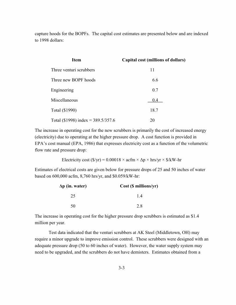
capture hoods for the BOPFs. The capital cost estimates are presented below and are indexed to 1998 dollars:

Item

Three venturi scrubbers

Three new BOPF hoods

Engineering

Miscellaneous

Total ($1990)

Total ($1998) index = 389.5/357.6

Capital cost (millions of dollars)

11

6.6

0.7

0.4

18.7

20

The increase in operating cost for the new scrubbers is primarily the cost of increased energy (electricity) due to operating at the higher pressure drop. A cost function is provided in EPA’s cost manual (EPA, 1986) that expresses electricity cost as a function of the volumetric flow rate and pressure drop:

Electricity cost ($/yr) = 0.00018 × acfm × ∆p × hrs/yr × $/kW-hr

Estimates of electrical costs are given below for pressure drops of 25 and 50 inches of water based on 600,000 acfm, 8,760 hrs/yr, and $0.059/kW-hr:

∆p (in. water) Cost ($ millions/yr)

25 1.4

50 2.8

The increase in operating cost for the higher pressure drop scrubbers is estimated as $1.4 million per year.

Test data indicated that the venturi scrubbers at AK Steel (Middletown, OH) may require a minor upgrade to improve emission control. These scrubbers were designed with an adequate pressure drop (50 to 60 inches of water). However, the water supply system may need to be upgraded, and the scrubbers do not have demisters. Estimates obtained from a

3-3

vendor indicated that two demisters for two 72-inch diameter stacks would cost about $7,000 (316 stainless steel chevrons). The cost of new water supply piping (EPA, 1986) for venturi scrubbers of this size was estimated as $10,600 for a total equipment cost of $17,600. Based on a retrofit factor of 1.3 and an indirect cost factor (from the cost manual [EPA, 1986]) of 36 percent of the purchased equipment cost, the total installed capital cost for the minor scrubber upgrade is estimated as $31,000.

3.4 Secondary Capture and Control Systems for Fugitive Emissions

Only one plant reported no controls for their casthouse—Gulf States Steel in Gadsden, Alabama. This plant may be able to use flame suppression and covered runners to provide adequate control to meet an opacity limit for the casthouse. However, a worst case approach is used by assuming that a capture system and baghouse may need to be installed. Based on the cost for such a system as reported by USS/Kobe Steel (Stinson, 1996), costs are estimated as an installed capital cost of $3.3 million, an operating cost of $0.7 million per year, and a total annualized cost of $1.0 million per year (includes capital recovery based on a 20-year life and 7 percent interest rate.)

AK Steel has a closed hood BOF shop in Middletown, OH that does not have a secondary capture and control system. The cost of a new system, including a baghouse control device, is estimated from the costs reported by two plants (Geneva Steel [Shaw, 1996] and AK Steel [Bradley, 1996] in Kentucky): capital cost of $3.4 million, an operating cost of $0.5 million per year, and a total annualized cost of $0.8 million per year (includes capital recovery based on a 20-year life and 7 percent interest rate.)

The MACT technology for secondary capture and control systems is a baghouse, and all plants except two use baghouses. Ispat-Inland and Bethlehem Steel (Burns Harbor, IN) use scrubbers as the control device for secondary emissions in the BOF shop. There is uncertainty about the level of emission control these scrubbers can achieve. As a worst case scenario we assume these scrubbers must be replaced by a baghouse at a capital cost of $3.4 million in these two plants. There would be no increase in operating cost (the operating cost for baghouses would be less than the current operating costs for the scrubbers).

3.5 Bag Leak Detection Systems

Each baghouse will be equipped with a bag leak detection system. These systems have an installed capital cost of $9,000 each with an annual operating cost of $500/year (EPA, 1998). There are approximately 88 baghouses at the 20 iron and steel plants.

3-4

Consequently, the total capital cost for bag leak detectors is $0.8 million with an annual operating cost of $44,000/year.

3.6 Total Nationwide Costs

The nationwide costs are summarized in Table 3-1 and, as described previously, may represent a worst case estimate because some of these plants may not have to install new controls. The nationwide total capital investment is estimated at $34 million, while the total annualized cost is estimated at $5.9 million per year with $3 million in annual capital costs and $2.9 million in annual operating and maintenance costs.

Table 3-1. Nationwide Cost of Proposed MACT Standard for Integrated Iron and Steel Mills: YEAR

Annual Annual Total Total Capital Operating Annual

Capital ($ ($ ($ Source ($ million) million/yr) million/yr) million/yr)

Gulf States, baghouse for casthouse 3.3 0.7 1.0

AK Steel (Middletown, OH), baghouse for 3.4 0.5 0.8 secondary BOF system

AK Steel, BOF scrubber upgrade 0.03 0 0.003

Ispat Inland, new primary scrubbers and hoods 20 1.4 3.3for No. 4 BOF shop (50 in. ∆p)

Ispat-Inland, baghouse to replace scrubber for secondary BOF system

3.4 0 0.3

Bethlehem, Burns Harbor, baghouse to replace scrubber for secondary BOF system

3.4 0 0.3

Bag leak detection systems 0.8 0.04 0.2

Total 34 3.0 2.6 5.9

3-5

SECTION 4

ECONOMIC IMPACT ANALYSIS

The proposed rule to control the release of HAPs from integrated iron and steel mill product operations will directly (through imposition of compliance costs) or indirectly (through changes in market prices) affect the entire U.S. iron and steel industry. Implementation of the proposed rule will increase the costs of producing steel mill products at affected facilities. As described in Section 3, these costs will vary across facilities and depend on their physical characteristics and baseline controls. The response by these producers to these additional costs will determine the economic impacts of the regulation. Specifically, the impacts will be distributed across producers and consumers of steel mill products and furnace coke through changes in prices and quantities in the affected markets. This section presents estimates of the economic impacts of the integrated iron and steel MACT using an economic model that captures the linkages between the steel mill products and furnace coke markets.

This section describes the data and approach used to estimate the economic impacts of this proposed rule for the baseline year of 1997. Section 4.1 presents the inputs for the economic analysis, including characterization of producers, markets, and the costs of compliance. Section 4.2 summarizes the conceptual approach to estimating the economic impacts on the affected industries. A fully detailed description of the economic impact methodology is provided in Appendix A. Lastly, Section 4.3 provides the results of the economic impact analysis.

4.1 EIA Data Inputs

Inputs to the economic analysis are a baseline characterization of directly and indirectly affected producers, their markets, and the estimated costs of complying with the proposed rule.

4.1.1 Producer Characterization

As detailed in Section 2, the baseline characterization of integrated and merchant manufacturing plants is based on the facility responses to EPA’s industry survey and industry

4-1

data sources. These plant-specific data on existing sources were supplemented with secondary information from the 1998 Directory of Iron and Steel Plants published by the Association of Iron and Steel Engineers and World Cokemaking Capacity published by the International Iron and Steel Institute, as well as mill-specific product supply equations for steel mill products (as described fully in Appendix A).

4.1.2 Market Characterization

Figure 4-1 summarizes the market interactions included in the Agency’s EIA modeling approach. Changes in the equilibrium price and quantity due to control costs on integrated iron and steel mills were estimated simultaneously in two linked markets:

` market for steel mill products and

` market for furnace coke.

As described in Section 2, steel mill products are supplied by three general groups: integrated iron and steel mills, nonintegrated steel mills (primarily mini-mills), and imports. Domestic consumers of steel mill products and exports account for the market demand. The market for steel mill products will be directly affected by the imposition of compliance costs on integrated mills.

In addition, as illustrated in Figure 4-1, the furnace coke market will be affected by the proposed regulation through changes in the derived demand from integrated mills producing steel mill products. Integrated mills’ market (and captive) demand for furnace coke depends on their production levels as influenced by the market for steel mill products. Integrated iron and steel mills that need more coke than their captive batteries can produce purchase furnace coke from the market. Many captive coke plants supply their excess coke to the furnace coke market. Merchant coke plants and foreign imports account for the remaining supply to the furnace coke market. Furnace coke produced at captive coke plants and shipped directly to integrated iron and steel mills owned by their parent companies does not directly enter the market for furnace coke.

Table 4-1 provides the 1997 data on the U.S. steel mill products and furnace coke markets used in this analysis. The market price for steel mill products was obtained from Current Industrial Reports (CIR) (U.S. DOC, 1997) and reflects the production-weighted average across all product types. The market price for furnace coke was determined, consistent with economic theory, by the highest-cost merchant producer. Domestic

4-2

Consumers of Steel Mill Products

Merchant Coke Plants

• Finishing Mills • Steelmaking Furnace • Blast Furnace

Captive Coke Plants

Imports

Imports

Exports

Integrated Iron and Steel Mills

Exports

Market for Furnace Coke

Control Costs

Market for Steel

Mill Products

Nonintegrated Steel Mills (including minimills)

Figure 4-1. Market Linkages Modeled in the Economic Impact Analysis

production from affected facilities reflects the aggregate of the plant-specific data presented in Section 2, while unaffected domestic production is derived either directly from secondary sources or as the difference between observed total U.S. production and the aggregate production from affected facilities. Foreign trade data were obtained from industry and government statistical publications supplemented by survey data. Market volumes for each product are then computed as the sum of U.S. production and foreign imports.

4.1.3 Regulatory Control Costs

As shown in Section 3, the Agency developed compliance costs based on plant characteristics and current controls at integrated iron and steel manufacturing facilities

4-3

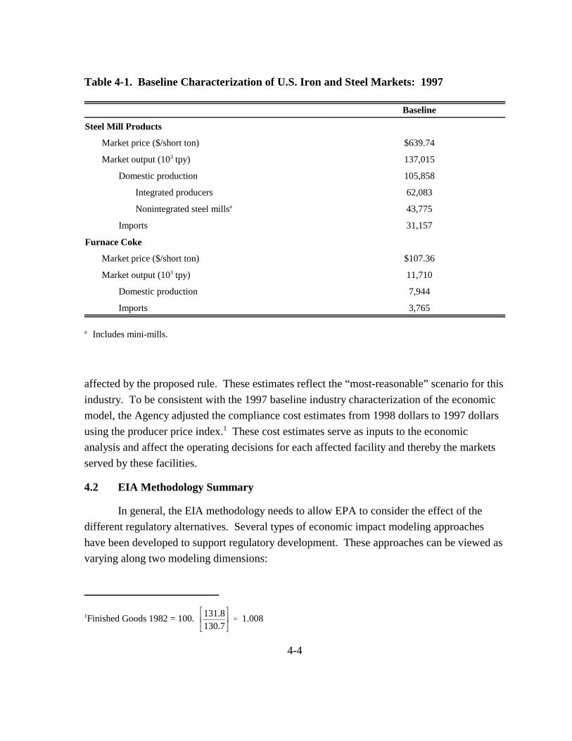
Table 4-1. Baseline Characterization of U.S. Iron and Steel Markets: 1997

Baseline

Steel Mill Products

Market price ($/short ton)

Market output (103 tpy)

Domestic production

Integrated producers

Nonintegrated steel millsa

Imports

Furnace Coke

Market price ($/short ton)

Market output (103 tpy)

Domestic production

Imports

$639.74

137,015

105,858

62,083

43,775

31,157

$107.36

11,710

7,944

3,765

a Includes mini-mills.

affected by the proposed rule. These estimates reflect the “most-reasonable” scenario for this industry. To be consistent with the 1997 baseline industry characterization of the economic model, the Agency adjusted the compliance cost estimates from 1998 dollars to 1997 dollars using the producer price index.1 These cost estimates serve as inputs to the economic analysis and affect the operating decisions for each affected facility and thereby the markets served by these facilities.

4.2 EIA Methodology Summary

In general, the EIA methodology needs to allow EPA to consider the effect of the different regulatory alternatives. Several types of economic impact modeling approaches have been developed to support regulatory development. These approaches can be viewed as varying along two modeling dimensions:

1Finished Goods 1982 = 100. 131.8 � 1.008

130.7

4-4

` the scope of economic decision making accounted for in the model and

` the scope of interaction between different segments of the economy.

Each of these dimensions was considered in selecting the approach used to model the economic impact of the proposed integrated iron and steel regulation.

To conduct the analysis for the proposed regulation, the Agency used a market modeling approach that incorporates behavioral responses in a multiple-market partial equilibrium model. Multiple-market partial equilibrium analysis provides a manageable approach to incorporating interactions between steel mill product and furnace coke markets into the EIA to better estimate the proposed regulation’s impact. The multiple-market partial equilibrium approach represents an intermediate step between a simple, single-market partial equilibrium approach and a full general equilibrium approach. The modeling technique is to link a series of standard partial equilibrium models by specifying the interactions between the supply and demand for products and then solving for changes in prices and quantities across all markets simultaneously. The EIA methodology is fully detailed in Appendix A.

The Agency’s methodology is soundly based on standard microeconomic theory relying heavily on previous economic analyses, employs a comparative static approach, and assumes certainty in relevant markets. For this analysis, prices and quantities are determined in perfectly competitive markets for steel mill products and furnace coke. The competitive model of price formation, as shown in Figure 4-2(a), posits that market prices and quantities are determined by the intersection of market supply and demand curves. Under the baseline scenario, a market price and quantity (P, Q) are determined by the downward-sloping market demand curve (DM) and the upward-sloping market supply curve (SM) that reflects the horizontal summation of the individual supply curves of directly affected and indirectly affected facilities that produce a given product.

With the regulation, the cost of production increases for directly affected producers. The imposition of the compliance costs is represented as an upward shift in the supply curve for each affected facility from Sa to Sak. As a result, the market supply curve shifts upward to SM

k as shown in Figure 4-2(b), reflecting the increased costs of production at these facilities. In the baseline scenario without the proposed standards, the industry would produce total output, Q, at the price, P, with affected facilities producing the amount qa and unaffected facilities accounting for Q minus qa, or qu. At the new equilibrium with the regulation, the market price increases from P to Pk, and market output (as determined from the market

4-5

p

Sa Su

p + = p

qa qu Q

Affected Facilities Unaffected Facilities Market

a) Baseline Equilibrium

p�

Sa S�a

p�

Su

p�

p + p = p

SM�

DM

SM

q�a qa qu q�u Q� Q

Affected Facilities Unaffected Facilities Market

b) With-Regulation Equilibrium

Figure 4-2. Market Equilibrium without and with Regulation

SM

DM

4-6

demand curve, DM) declines from Q to Qk. This reduction in market output is the net result from reductions at affected facilities and increases at unaffected facilities.

4.3 Economic Impact Results

Based on the simple analytics presented above, when faced with higher costs of production, producers will attempt to mitigate the impacts by making adjustments to shift as much of the burden on other economic agents as market conditions allow. The adjustments available to facility operators include changing production processes, changing inputs, changing output rates, or even closing the facility. This analysis focuses on the last two options because they appear to be the most viable for manufacturing facilities, at least in the near term. Because the regulation will affect a large segment of the steel mill products market, we expect upward pressure on prices as integrated producers reduce output rates in response to higher costs. Higher prices reduce quantity demanded and output for each market product, leading to changes in profitability of batteries, facilities, and firms. These market and industry adjustments will also determine the social costs of the regulation and its distribution across stakeholders (producers and consumers).

To estimate these impacts, the economic modeling approach described in Appendix A was operationalized in a multiple spreadsheet model. This model characterizes those producers and consumers identified in Figure 4-1 and their behavioral responses to the imposition of the regulatory compliance costs. These costs are expressed per ton of steel mill product and serve as the input to the economic model, or “cost-shifters” of the baseline supply curves at affected facilities.

In addition to the “cost-shifters” the other major factors that influence behavioral adjustments in the model are the supply and demand elasticities of producers and consumers. Table 4-2 presents the key elasticity parameters used in the model. Specific functional forms are presented in Appendix A. Given these costs and supply and demand elasticities, the model determines a new equilibrium solution in a comparative static approach. The following sections provide the Agency’s estimates of the resulting economic impacts for the proposed rule.

4.3.1 Market-Level Impacts

The increased cost of steel mill product production due to the regulation is expected to slightly increase the price of steel mill products and reduce their production and consumption from 1997 baseline levels. As shown in Table 4-3, the regulation is projected to

4-7

Table 4-2. Supply and Demand Elasticities Used in Analysis

Market Supply Elasticity Demand Elasticity Furnace Coke

Domestic Calculated Derived Foreign 3.0a –0.3a

Steel Mill Products Domestic 1.0b –0.59c

Foreign 1.0b –1.0b

a Graham, Thorpe, and Hogan (1999). b Assumed value.

Weighted average of product demand elasticities estimated in econometric analysis.

increase the price of steel mill products less than 0.01 percent, or $0.01 per short ton. Because the change in the demand for furnace coke is very small, the entire market impact is absorbed by a single battery that is assumed to have a constant marginal cost. As a result, market output of furnace coke declines slightly but the market price remains unchanged. See Appendix B for a detailed description of the step wise supply function for the furnace coke market. This in turn leads to no change in the level of imports (or exports) of furnace coke. As expected, directly affected steel mill product output declines across integrated producers, while supply from domestic and foreign producers not subject to the regulation increases. The resulting net declines are slight across both products (i.e., less than 0.01 percent decline in market output).

4.3.2 Industry-Level Impacts

Industry revenue, costs, and profitability change as prices and production levels adjust to increased production costs. As shown in Table 4-4, the economic model projects that profits for directly affected integrated iron and steel producers will decrease by $5.2 million, or 0.4 percent. In addition, the Agency projects no change in profits for furnace coke plants because the small reduction in output comes from the marginal coke battery, which by assumption has zero profit in baseline. Those domestic suppliers not subject to the regulation experience small gains; nonintegrated steel mills (i.e., mini-mills) increase profits by $0.6 million.

4-8

c

Table 4-3. Market-Level Impacts of the Proposed Integrated Iron and Steel MACT: 1997

Changes From Baseline

Baseline Absolute Percent

Steel Mill Products

Market price ($/short ton)

Market output (103 tpy)

Domestic production

Integrated producers

Nonintegrated steel millsa

Imports

Furnace Coke

Market price ($/short ton)

Market output (103 tpy)

Domestic production

Imports

$639.74 $0.01 <0.01%

137,015 –1.6 <–0.01%

105,858 –2.3 <–0.01%

62,083 –3.1 <–0.01%

43,775 0.9 <0.02%

31,157 0.6 <0.02%

$107.36 $0.00 0.00%b

11,710 –0.1 <–0.01%

7,944 –0.1 <–0.01%

3,765 0.0 0.00%b

a Includes mini-mills. b The market for furnace coke is virtually unaffected by the regulation. The entire market impact is absorbed

by a single battery that is assumed to have a constant marginal cost. As a result, market output of furnace coke declines slightly but the market price remains unchanged.

4.3.2.1 Changes in Profitability

For integrated steel mills, operating profits decline by $5.2 million. This is the net result of three effects:

` Net decrease in revenue ($1.1 million): Steel mill product revenue decreases as a result of reductions in output. However, these losses were mitigated by increased revenues from furnace coke supplied to the market as a result of decreased internal demand for captive coke production for selected integrated iron and steel plants.

` Net decrease in production costs ($1.9 million): Reduction in steel mill product and market coke production costs occur as output declines.

4-9

Table 4-4. National-Level Industry Impacts of the Proposed Integrated Iron and Steel MACT: 1997

Changes From Baseline Baseline Absolute Percent

Integrated Iron and Steel Mills Total revenues ($106/yr)

Steel mill products Market coke operations

Total costs ($106/yr) Control costs

Steel production Captive coke production Market coke production

Production costs Steel production Captive coke production Market coke consumption Market coke production

Operating profits ($106/yr) Iron and steel facilities (#) Coke batteries (#) Employment (FTEs) Coke Producers (Merchant Only) Furnace

Revenues ($106/yr) Costs ($106/yr)

Control costs Production costs

Operating profits ($106/yr) Coke batteries (#) Employment (FTEs) Nonintegrated Steel Millsa

Operating profits ($106/yr)

$40,223.9 –$1.09 <0.01% $39,716.9 –$1.21 <0.01%

$507.0 $0.12 0.02% $38,834.7 $4.07 0.01%

$0.0 $5.94 NA $0.0 $5.94 NA $0.0 $0.00 NA $0.0 $0.00 NA

$38,834.7 –$1.88 <–0.01% $36,290.1 –$1.87 –0.01%

$942.5 –$0.12 –0.01% $1,167.8 –$0.01 <–0.01%

$434.3 $0.12 0.03% $1,389.1 –$5.16 –0.37%

20 0 0.00% 37 0 0.00%

67,198 –6 –0.01%

$366.5 –$0.15 –0.04% $318.5 –$0.15 –0.05%

$0.0 $0.00 NA $318.5 –$0.15 –0.05% $48.0 $0.00 0.00%

13 0 0.00% 840 –1 –0.12%

NA $0.6 NA

a Includes mini-mills.

4-10

Increase in control costs ($5.9 million): The costs of captive production of furnace coke increase as a result of regulatory controls.

Industry-wide profits for merchant furnace coke producers are projected to remain unchanged as a result of the following:

` Decreases in revenue ($0.2 million): Reductions in output result in decreased revenue.

` Reduction in production costs ($0.2 million): Reduction in coke production costs occurs as output declines.

Additional distributional impacts of the rule within each producer segment are not necessarily apparent from the reported decline or increase in their aggregate operating profits. The regulation creates both gainers and losers within each industry segment based on the distribution of compliance costs across facilities. As shown in Table 4-5, a substantial set of directly affected integrated iron and steel facilities (i.e., 16 plants, or 80 percent) are projected to become more profitable with the regulation with a total gain of $0.5 million as they benefit from higher steel mill product prices. However, four integrated mills are projected to experience a total profit loss of $5.6 million. These integrated plants have higher per-unit costs ($0.41 per ton) relative to the facilities that experience profit gains.

4.3.2.2 Facility Closures

EPA estimates no integrated iron or steel facility is likely to prematurely close as a result of the regulation. In addition, no furnace coke batteries are projected to cease operations as a result of decreased demand for furnace coke resulting from the regulation.

4.3.2.3 Changes in Employment

As a result of decreased output levels, industry employment is projected to decrease by less than 0.5 percent, or seven full-time equivalents (FTEs), with the regulation. This is the net result of employment losses for integrated iron and steel mills totaling six FTEs and merchant coke plants of one FTEs. Although EPA projects increases in output for producers not subject to the rule, which would likely lead to increases in employment, the Agency did not develop quantitative estimates for this analysis.

4-11

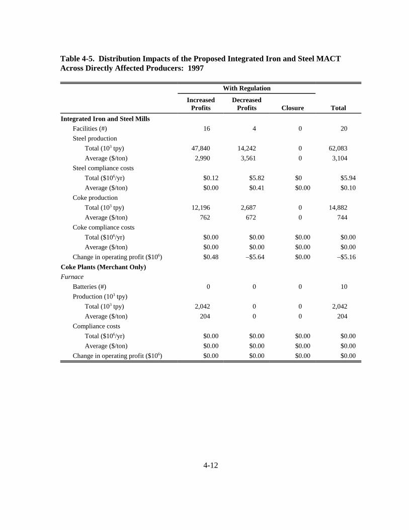
Table 4-5. Distribution Impacts of the Proposed Integrated Iron and Steel MACT Across Directly Affected Producers: 1997

With Regulation

Increased Decreased Profits Profits Closure Total

Integrated Iron and Steel Mills Facilities (#) Steel production

Total (103 tpy) Average ($/ton)

Steel compliance costs Total ($106/yr) Average ($/ton)

Coke production Total (103 tpy) Average ($/ton)

Coke compliance costs Total ($106/yr) Average ($/ton)

16 4 0 20

47,840 14,242 0 62,083 2,990 3,561 0 3,104

$0.12 $5.82 $0 $5.94 $0.00 $0.41 $0.00 $0.10

12,196 2,687 0 14,882 762 672 0 744

$0.00 $0.00 $0.00 $0.00 $0.00 $0.00 $0.00 $0.00

Change in operating profit ($106) $0.48 –$5.64 $0.00 –$5.16 Coke Plants (Merchant Only) Furnace

Batteries (#) 0 0 0 10 Production (103 tpy)

Total (103 tpy) 2,042 0 0 2,042 Average ($/ton) 204 0 0 204

Compliance costs Total ($106/yr) $0.00 $0.00 $0.00 $0.00 Average ($/ton) $0.00 $0.00 $0.00 $0.00

Change in operating profit ($106) $0.00 $0.00 $0.00 $0.00

4-12

4.3.3 Social Cost

The social impact of a regulatory action is traditionally measured by the change in economic welfare that it generates. The social costs of the proposed rule will be distributed across consumers and producers alike. Consumers experience welfare impacts due to changes in market prices and consumption levels associated with the rule. Producers experience welfare impacts resulting from changes in profits corresponding with the changes in production levels and market prices. However, it is important to emphasize that this measure does not include benefits that occur outside the market, that is, the value of reduced levels of air pollution with the regulation.

The national compliance cost estimates are often used as an approximation of the social cost of the rule. The engineering analysis estimated annual costs of $5.94 million. In this case, the burden of the regulation falls solely on the affected facilities that experience a profit loss exactly equal to these cost estimates. Thus, the entire loss is a change in producer surplus with no change (by assumption) in consumer surplus. This is typically referred to as a “full-cost absorption” scenario in which all factors of production are assumed to be fixed and firms are unable to adjust their output levels when faced with additional costs.

In contrast, the economic analysis conducted by the Agency accounts for behavioral responses by producers and consumers to the regulation (i.e., shifting costs to other economic agents). This approach results in a social cost estimate that may differ from the engineering estimate and also provides insights on how the regulatory burden is distributed across stakeholders. As shown in Table 4-6, the economic model estimates the total social cost of the rule to be $5.94 million. Although society reallocates resources as a result of the increased cost of steel mill product production, only a very small difference occurs.

In the final product markets, higher market prices lead to consumers of steel mill products experiencing losses of $1.7 million. Although integrated iron and steel producers are able to pass on a limited amount of cost increases to their final consumers (e.g., automotive manufacturers and the construction industry), the increased costs result in a net decline in profits at integrated mills of $5.2 million.

In the coke industry, furnace coke profits at merchant plants are projected to remain unchanged, as reductions in output come from the marginal merchant furnace coke battery. Lastly, domestic producers not subject to the regulation (i.e., nonintegrated steel mills and

4-13

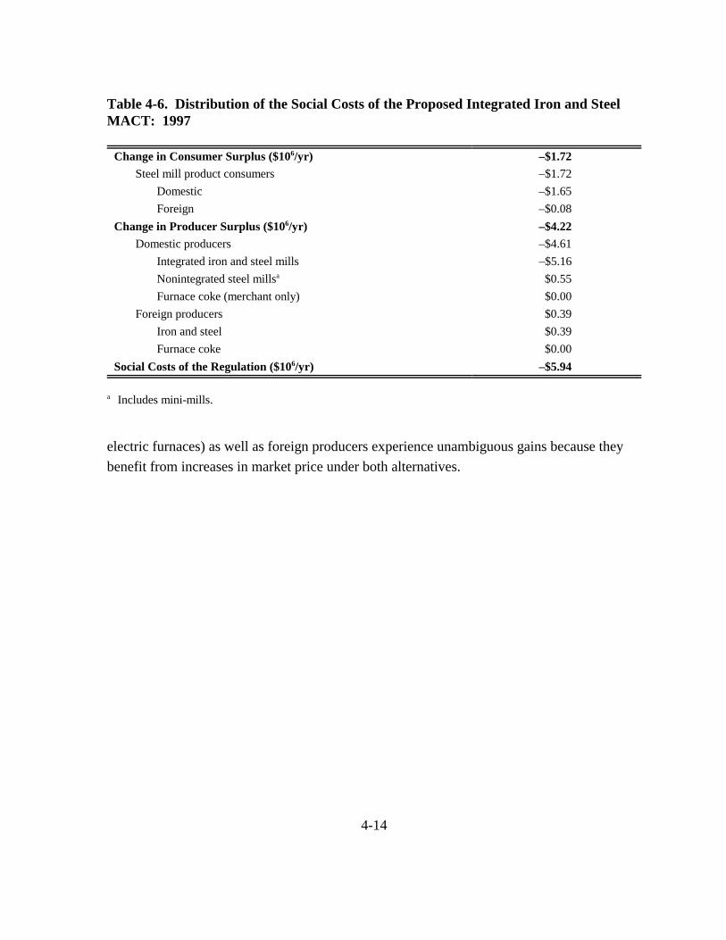
Table 4-6. Distribution of the Social Costs of the Proposed Integrated Iron and Steel MACT: 1997

Change in Consumer Surplus ($106/yr) Steel mill product consumers

Domestic Foreign

Change in Producer Surplus ($106/yr) Domestic producers

Integrated iron and steel mills Nonintegrated steel millsa

Furnace coke (merchant only) Foreign producers

Iron and steel Furnace coke

Social Costs of the Regulation ($106/yr)

–$1.72 –$1.72 –$1.65 –$0.08 –$4.22 –$4.61 –$5.16 $0.55 $0.00 $0.39 $0.39 $0.00

–$5.94

a Includes mini-mills.

electric furnaces) as well as foreign producers experience unambiguous gains because they benefit from increases in market price under both alternatives.

4-14

SECTION 5

SMALL BUSINESS IMPACTS

The Regulatory Flexibility Act (RFA) of 1980 as amended in 1996 by the Small Business Regulatory Enforcement Fairness Act (SBREFA) generally requires an agency to prepare a regulatory flexibility analysis of a rule unless the agency certifies that the rule will not have a significant economic impact on a substantial number of small entities. Small entities include small businesses, small organizations, and small governmental jurisdictions.

For purposes of assessing the impacts of the proposed rule on small entities, a small entity is defined as: (1) a small business according to SBA size standards for NAICS code 331111 (i.e., Iron and Steel Mills) of 1,000 or fewer employees; (2) a small governmental jurisdiction that is a government of a city, county, town, school district or special district with a population of less than 50,000; and (3) a small organization that is any not-for-profit enterprise that is independently owned and operated and is not dominant in its field.

Based on the above definition of small entities and the company-specific employment data from Section 2 of this report, the Agency has determined that no small businesses within this source category would be subject to this proposed rule. Therefore, because this proposed rule will not impose any requirements or additional costs on small entities, this action will not have a significant economic impact on a substantial number of small entities.

5-1

REFERENCES

American Iron and Steel Institute (AISI). 1989a. Steelmaking Flowlines. Washington, DC: AISI.

American Iron and Steel Institute (AISI). 1989b. Steel Processing Flowlines. Washington, DC: AISI.

American Iron and Steel Institute (AISI). 1990-1998. Annual Statistical Report. Washington, DC: AISI.

American Iron and Steel Institute (AISI). “The Steel Packaging Solution for Quality and Performance.” <http://www.steel.org>. As obtained on August 19, 1998.

American Metal Market. 1998. “AMM Online.”

Association of Iron and Steel Engineers (AISE). 1998. 1998 Directory Iron and Steel Plants. Pittsburgh, PA: AISE.

Associated Press (AP). February 12, 1999. “Brazil and Japan Dumped Steel, U.S. Finds.”

Autosteel. “Cutting Costs.” <http://www.autosteel.org>. Accessed August 19, 1998a.

Berry, Brian. Jan. 1997. “The Challenge for Integrated Mills.” New Steel.

Bingham, T.H., and T.J. Fox. 1999. “Model Complexity and Scope for Policy Analysis.” Public Administration Quarterly 23(3).

Bradley, L. January 1996. “AK Steel’s Response to Pollution Control Equipment Cost Survey.”

Business Communications Company. October 1995. “The Future of the Steel Industry in the U.S.”

Carson, J. 2000. No. 4 BOF Gas Cleaning Upgrade (dated September 9, 1990). Provided on April 6, 2000.

Dun & Bradstreet. 1998. Dun’s Market Identifier Electronic Database. Dialog Corporation.

EIU. September 1993. “The Material Revolution in the Motor Industry.” The Dialog Corporation. <http://www.profound.com>.

Engineering and Mining Journal. 1997. “A New U.S. Trend? No Leftovers—No Problems.” 198(10):WW15.

R-1

Fenton, Michael. U.S. Geological Survey, Minerals Information: Iron and Steel Scrap. 1996. <http://minerals.er.usgs.gov/minerals/pubs/commodity/iron_&_steel/350496.pdf>. .

Furukawa, Tsukasa. March 1998. “Japan’s Search for ‘Ultra Steel’.” New Steel.

Hogan, William T., and Frank T. Koelble. 1996. “Steel’s Coke Deficit: 5.6 Million Tons and Growing.” New Steel 12(12):50-59.

Lankford, William T., Norman L. Samways, Robert F. Craven, and Harold E. McGannon, eds. 1985. The Making, Shaping and Treating of Steel. Pittsburgh: United States Steel, Herbick & Held.

Paxton, H.W., and A.J. DeArdo. January 1997a. “Steel vs. Aluminum, Plastic, and the Rest.” New Steel.

Paxton, H.W. and A.J. DeArdo. February 1997b. “What’s Driving the Change in Materials.” New Steel.

Prabhu, H.W., and P.F. Cilione. 1992. “1990 Clean Air Act Amendments: Technical/Economic Impacts.” Iron and Steel Engineer 69(1):33-44.

Ritt, Adam. June 1998. “The Pressure to Go Global.” New Steel.

Samways, Norman L. February 1998. “Developments in the North American Iron and Steel Industry—1997.” Iron and Steel Engineer.

Shaw, K.C. January 26, 1996. “Geneva Steel’s Response to Pollution Control Equipment Cost Survey.”

The Steel Alliance. “Ultralight Steel Auto Body.” <http://www.thenewsteel.org>. As obtained on August 19, 1998.

Steel Recycling Institute. 2000a. “Steel Construction: Building for the Future.”

Steel Recycling Institute. 2000b. “Recycling Steel Appliances.” <http://www.recycle-steel.org>.

Stinson, R. March 6, 1996. USS/Kobe Steel’s Response to Pollution Control Equipment Cost Survey.

U.S. Bureau of the Census. 1988-1998. Current Industrial Reports: Steel Mill Products MA33B.<http://www.census.gov/cir/www/ma33b.html>.

U.S. Bureau of the Census. 1997. Statistical Abstact of the United States. [computer file]. <http:www.census.gov/prod/www/abs/cc97stab.html>. Last updated July 27, 1999.

U.S. Bureau of the Census. 1998. Current Construction Reports—Value of Construction Put in Place: May 1998. Washington, DC: Government Printing Office.

R-2

U.S. Bureau of Economic Analysis. Summary National Income and Product Time Series, 1929-1997. [computer file]. <http://www.BEA.DOC.gov/bea/dn1.htm>. Last updated December 18, 1998.

U.S. Bureau of Labor Statistics. BLS LABSTAT Database: Employment and Earnings, SIC 33. <http://www.bls.gov>. Obtained in September 1998.

U.S. Department of Energy, Energy Information Administration. 1990. Quarterly Coal Report October - December. Washington, DC: Government Printing Office.

U.S. Department of Energy, Energy Information Administration. 1998. Coal Industry Annual 1997. Washington, DC: Government Printing Office.

U.S. Environmental Protection Agency (EPA). 1979. Technical Approach for a Coke Production Cost Model. Research Triangle Park, NC: Research Triangle Institute.

U.S. Environmental Protection Agency (EPA). September 1986. Handbook: Control Technologies for Hazardous Air Pollutants. EPA/626/6-86/014.

U.S. Environmental Protection Agency (EPA). 1988. Benzene Emissions from Coke By-Product Recovery Plants-Background Information for Proposed Standards. Research Triangle Park, NC: Office of Air Quality Planning and Standards.

U.S. Environmental Protection Agency (EPA). 1991. Controlling Emissions from By-Product Coke Oven Charging, Door Leaks, and Topside Leaks: An Economic Impacts Analysis. Research Triangle Park, NC: Research Triangle Institute.

U.S. Environmental Protection Agency, Office of Compliance. 1995. EPA Office of Compliance Sector Notebook Project: Profile of the Iron and Steel Industry. Washington, DC: Environmental Protection Agency.

U.S. Environmental Protection Agency (EPA). April 1998a. “Supporting Statement for the Primary Lead MACT Information Collection Request.”

U.S. Environmental Protection Agency. 1998b. Update of Integrated Iron and Steel Industry Responses to Information Collection Request (ICR) Survey. Database prepared for EPA’s Office of Air Quality Planning and Standards. Research Triangle Park, NC: Environmental Protection Agency.

U.S. Environmental Protection Agency (EPA). 1999. OAQPS Economic Analysis Resource Document. Durham, NC: Innovative Strategies and Economics Group.

U.S. Geological Survey. 1987-1990. Aluminum Statistical Compendium. <http:minerals. usgs.gov/minerals/pubs/commodity/aluminum/index.html>. Last updated September 5, 1998.

U.S. Geological Survey. 1995-1997. Minerals Yearbook. <http:minerals.usgs.gov/ minerals/pubs/commodity/aluminum/index.html>. Last updated September 5, 1998.

R-3

U.S. Geological Survey. 1998. Mineral Commodity Summaries. Reston, VA: USGS. <http:minerals.usgs.gov/minerals/pubs/commodity/aluminum/index.html>.

U.S. International Trade Commission. 1994. Metallurgical Coke: Baseline Analysis of the U.S. Industry and Imports. Publication No. 2745. Washington, DC: U.S. International Trade Commission.

U.S. International Trade Commission. July 2000. “Foundry Coke: A Review of the Industries in the United States and China.” <http://www.usitc.gov/sec/ I0917W1.htm>.

Woker, Craig. September 1998. “The Next Wave of Coating Lines.” New Steel.

The World Bank. 1994. Market Outlook for Major Energy Products, Metals, and Minerals. Washington, DC: The World Bank.

R-4

APPENDIX A

ECONOMIC IMPACT ANALYSIS METHODOLOGY

This appendix provides the methodology for analyzing the economic impacts of the proposed MACT standard for coke ovens. Implementation of this methodology provided the economic data and supporting information that EPA requires to support its regulatory determination. This approach is firmly rooted in microeconomic theory and the methods developed for earlier EPA studies to operationalize this theory. The Agency employed a computerized market model of the coke, steel mill products, and iron castings industries to estimate the behavioral responses to the imposition of regulatory costs and, thus, the economic impacts of the proposed standard. The market model captures the linkages between these industries through changes in equilibrium prices and quantities. The same model is used to evaluate the economic impact of the proposed integrated iron and steel facilities MACT and iron foundries MACT to ensure consistency across the EIAs for these MACT standards.

This methodology section describes the conceptual approach selected for this EIA. For each product market included in the analysis, EPA derived facility-level supply and demand functions that are able to account for the behavioral response and market implications of the regulation’s costs. Finally, this appendix presents an overview of the specific functional forms that constitute the Agency’s computerized market model.

A.1 Overview of Economic Modeling Approach

In general, the EIA methodology needs to allow EPA to consider the effect of the different regulatory alternatives. Several types of economic impact modeling approaches have been developed to support regulatory development. These approaches can be viewed as varying along two modeling dimensions:

` the scope of economic decision making accounted for in the model, and

` the scope of interaction between different segments of the economy.

A-1

Each of these dimensions was considered in selecting the approach used to model the economic impact of the proposed coke regulation. Bingham and Fox (1999) provide a useful summary of these dimensions as they relate to modeling the outcomes of environmental regulations.

For this analysis, prices and quantities are determined in perfectly competitive markets for furnace coke, foundry coke, finished steel mill products, and iron castings. The Agency analyzed the impact of the proposed regulation using a market modeling approach that incorporates behavioral responses in a multiple-market partial equilibrium model. Multiple-market partial equilibrium analysis accounts for the interactions between coke, steel mill product, and iron castings markets into the EIA to better estimate the proposed regulation’s impact. The modeling technique is to link a series of standard partial equilibrium models by specifying the interactions between the supply and demand for products and then solving for changes in prices and quantities across all markets simultaneously.

Figure A-1 summarizes the market interactions included in the Agency’s EIA modeling approach. Changes in the equilibrium price and quantity due to control costs on coke batteries were estimated simultaneously in four linked markets:

` market for furnace coke,

` market for foundry coke,

` market for steel mill products, and

` market for iron castings.

As described in Section 2 of this EIA report, many captive coke plants supply their excess furnace coke to the market. Merchant coke plants and foreign imports account for the remaining supply to the furnace coke market. Furnace coke produced at captive coke plants and shipped directly to integrated iron and steel mills owned by their parent companies does not directly enter the market for furnace coke. However, compliance costs incurred by these captive, or “in-house,” furnace coke batteries indirectly affect the furnace coke market through price and output changes in the steel mill products market.

The market demand for furnace coke is derived from integrated mills producing steel mill products. Integrated iron and steel mills that need more coke than their captive batteries can produce will purchase furnace coke from the market. Integrated mills’ market demand

A-2

Consumers of Steel Consumers of Mill Products Iron Castings

Merchant Coke Plants

• Finishing Mills • Steelmaking Furnace • Blast Furnace

Captive Coke Plants

Market for Foundry Coke

Imports

Imports

Exports

Integrated Iron and Steel Mills

Exports

Market for Furnace Coke

Electric Furnaces

Cupola Furnaces

Control Costs Coke MACT

Market for Steel

Mill Products

Nonintegrated Steel Mills (including minimills)

Market for Iron Castings

Imports

Exports

Control Costs Iron and Steel Foundry MACT

Control Costs Integrated Iron

and Steel MACT

Figure A-1. Market Linkages Modeled in the Economic Impact Analysis

for furnace coke depends on their production levels as influenced by the market for steel mill products. Steel mill products are supplied by three sources: integrated iron and steel mills, nonintegrated steel mills (primarily mini-mills), and imports. Domestic consumers of steel mill products and exports account for the market demand.

As described in Section 2 of this EIA report, in the analysis baseline of 1997, merchant plants are the sole suppliers of foundry coke to the market. The U.S. International Trade Commission (2000) has documented an increasing trend in foreign imports of foundry coke from China; however, these Chinese imports represented less than 1 percent of U.S. foundry coke consumption in 1997. Moreover, the USITC report indicates that the inferior quality of imported foundry coke and future environmental regulations being proposed in China may limit the market penetration in the United States. Consumers of foundry coke include foundries with cupolas that produce iron castings that are modeled using a single, representative demand curve.

A-3

In addition to furnace and foundry coke, merchant and captive coke plants sell a by-product referred to as “other coke” that is purchased as a fuel input by cement plants, chemical plants, and nonferrous smelters. Because “other coke” is a by-product and represented only 2 percent of U.S. coke production in 1997 it is not formally characterized by supply and demand in the market model. Revenues from this product are accounted for by assuming its volume is a constant proportion of the total amount of coke produced by a battery and sold at a constant price.

A.2 Conceptual Market Modeling Approach

This section examines the impact of the regulations on the production costs of coke for affected facilities, both merchant and captive. It provides an overview of the basic economic theory of the effect of regulations on facility production decisions and the concomitant effect on market outcomes. Following the OAQPS Economic Analysis Resource Document (EPA, 1999), we employed standard concepts in microeconomics to model the supply of affected products and the impacts of the regulations on production costs and the operating decisions. The approach relies heavily on previous economic analyses, employs a comparative static approach, and assumes certainty in relevant markets. The three main elements of the analysis are regulatory effects on the manufacturing facility, market responses, and facility–market interactions. The remainder of this section describes each of these main elements.

A.2.1 Facility-level Responses to Control Costs

Individual plant-level production decisions were modeled to develop the market supply and demand for key industry segments in the analysis. Production decisions were modeled as intermediate-run decisions, assuming that the plant size, equipment, and technologies are fixed. For example, the production decision typically involves (1) whether a firm with plant and equipment already in place purchases inputs to produce output and (2) at what capacity utilization the plant should operate. A profit-maximizing firm will operate existing capital as long as the market price for its output exceeds its per-unit variable production costs, since the facility will cover not only the cost of its variable inputs but also part of its capital costs. Thus, in the short run, a profit-maximizing firm will not pass up an opportunity to recover even part of its fixed investment in plant and equipment.

The existence of fixed production factors gives rise to diminishing returns to those fixed factors and, along with the terms under which variable inputs are purchased, defines the

A-4

upward-sloping form of the marginal cost (supply) curve employed for this analysis. Figure A-2 illustrates this derivation of the supply function at an individual mill based on the classical U-shaped cost structure. The MC curve is the marginal cost of production, which intersects the facility’s average variable (avoidable) cost curve (AVC) and its average total cost curve (ATC) at their respective minimum points. The supply function is that portion of the marginal cost curve bounded by the minimum economically feasible production rate (qm) and the technical capacity (qM). A profit-maximizing producer will select the output rate where marginal revenue equals price, that is, at [P*, q*]. If market price falls below ATC, then the firm’s best response is to cease production because total revenue does not cover total costs of production.

$/q

P

AVC

ATC

MC

qm q qM q/t

Figure A-2. Product Supply Function at Facility

Now consider the effect of the proposed regulation and the associated compliance costs. These fall into one of two categories: avoidable variable and avoidable nonvariable. These proposed costs are characterized as avoidable because a firm can choose to cease operation of the facility and, thus, avoid incurring the costs of compliance. The variable control costs include the operating and maintenance costs of the controls, while the nonvariable costs include compliance capital equipment. Figure A-3 illustrates the effect of

A-5

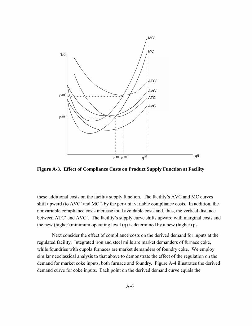
$/q

P m′

P m

MC

MC′

ATC�

AVC′

ATC

AVC

q m q m′ q M q/t

Figure A-3. Effect of Compliance Costs on Product Supply Function at Facility

these additional costs on the facility supply function. The facility’s AVC and MC curves shift upward (to AVCk and MCk) by the per-unit variable compliance costs. In addition, the nonvariable compliance costs increase total avoidable costs and, thus, the vertical distance between ATCk and AVCk. The facility’s supply curve shifts upward with marginal costs and the new (higher) minimum operating level (q) is determined by a new (higher) ps.

Next consider the effect of compliance costs on the derived demand for inputs at the regulated facility. Integrated iron and steel mills are market demanders of furnace coke, while foundries with cupola furnaces are market demanders of foundry coke. We employ similar neoclassical analysis to that above to demonstrate the effect of the regulation on the demand for market coke inputs, both furnace and foundry. Figure A-4 illustrates the derived demand curve for coke inputs. Each point on the derived demand curve equals the

A-6

$/qy

1 yD

Dy

q/ty

Figure A-4. Derived Demand Curve for Coke Inputs

willingness to pay for the corresponding marginal input. This is typically referred to as the input’s value of marginal product (VMP), which is equal to the price of the output (P) less the per-unit compliance cost (c) times the input’s “marginal physical product” (MPP), which is the incremental output attributable to the incremental inputs. If, as assumed in this analysis, the input-output relationship between the market coke input and the final product (steel mill products or iron castings) is strictly fixed, then the VMP of the market coke is constant and the derived demand curve is horizontal with the constant VMP as the vertical intercept, as shown in Figure A-4. Ignoring any effect on the output price for now, an increase in regulatory costs will lower the VMP of all inputs leading to a downward shift in the derived

demand in Figure A-4 from Dy to Dy1 .

A.2.2 Market Effects

To evaluate the market impacts, the economic analysis assumes that prices and quantities are determined in a competitive market (i.e., individual facilities have negligible power over the market price and thus take the price as “given” by the market). As shown in Figure A-5(a), under perfect competition, market prices and quantities are determined by the intersection of market supply and demand curves. The initial baseline scenario consists of a market price and quantity (P, Q) that is determined by the downward-sloping market demand

A-7

p

Sa Su

p + = p

qa qu Q

Affected Facilities Unaffected Facilities Market

a) Baseline Equilibrium

p�

Sa S�a

p�

Su

p�

p + p = p

SM�

DM

SM

q�a qa qu q�u Q� Q

Affected Facilities Unaffected Facilities Market

b) With-Regulation Equilibrium

Figure A-5. Market Equilibrium without and with Regulation

SM

DM

A-8

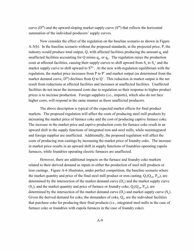
curve (DM) and the upward-sloping market supply curve (SM) that reflects the horizontal summation of the individual producers’ supply curves.

Now consider the effect of the regulation on the baseline scenario as shown in Figure A-5(b). In the baseline scenario without the proposed standards, at the projected price, P, the industry would produce total output, Q, with affected facilities producing the amount qa and unaffected facilities accounting for Q minus qa, or qu. The regulation raises the production costs at affected facilities, causing their supply curves to shift upward from Sa to Sak and the market supply curve to shift upward to SM

k. At the new with-regulation equilibrium with the regulation, the market price increases from P to Pk and market output (as determined from the market demand curve, DM) declines from Q to Qk. This reduction in market output is the net result from reductions at affected facilities and increases at unaffected facilities. Unaffected facilities do not incur the increased costs due to regulation so their response to higher product prices is to increase production. Foreign suppliers (i.e., imports), which also do not face higher costs, will respond in the same manner as these unaffected producers.

The above description is typical of the expected market effects for final product markets. The proposed regulation will affect the costs of producing steel mill products by increasing the market price of furnace coke and the cost of producing captive furnace coke. The increase in the market price and captive production costs for furnace coke result in an upward shift in the supply functions of integrated iron and steel mills, while nonintegrated and foreign supplier are unaffected. Additionally, the proposed regulation will affect the costs of producing iron castings by increasing the market price of foundry coke. The increase in market price results in an upward shift in supply functions of foundries operating cupola furnaces, while foundries operating electric furnaces are unaffected.

However, there are additional impacts on the furnace and foundry coke markets related to their derived demand as inputs to either the production of steel mill products or iron castings. Figure A-6 illustrates, under perfect competition, the baseline scenario where the market quantity and price of the final steel mill product or iron casting, Qx(Qx0, Px0), are determined by the intersection of the market demand curve (Dx) and the market supply curve (Sx), and the market quantity and price of furnace or foundry coke, Qy(Qy0, Py0), are determined by the intersection of the market demand curve (Dy) and market supply curve (Sy). Given the derived demand for coke, the demanders of coke, Qy, are the individual facilities that purchase coke for producing their final products (i.e., integrated steel mills in the case of furnace coke or foundries with cupola furnaces in the case of foundry coke).

A-9

$/Qx

Px1

Px0

Sx�

Sx

Dx

Qx1 Qx0 Qx/t

(a) Market for single steel mill product or iron casting, Qx

$/Qy Sy

Dy

Sy

Dy ′′

Dy ′

Dy ′′ ′

′

Py2 Py3 = Py0

Py1

Qy1 Qy3 Qy2 Qy0 Qy/t

(b) Market for coke input, Qy

Figure A-6. Market Equilibria With and Without Compliance Costs

A-10

Imposing the regulations increases the costs of producing coke and, thus, the final product, shifting the market supply functions for both commodities upward to Sxk and Syk, respectively. The supply shift in the final product market causes the market quantity to fall to Qx1 and the market price to rise to Px1 in the new equilibrium. In the market for coke, the reduced production of the final product causes a downward shift in the demand curve (Dy) with an unambiguous reduction in coke production, but the direction of the change in market price is determined by the relative magnitude of the demand and supply shift. If the downward demand effect dominates, the price will fall (e.g., Py1); however, if the upward supply effect dominates, the price will rise (e.g., Py2). Otherwise, if the effects just offset each other, the price remains unchanged (e.g., Py3 = Py0).

A.2.3 Facility-Level Responses to Compliance Costs and New Market Prices

In evaluating the market effects, we must distinguish between the initial effect of the regulations and the net effect after all markets have adjusted. The profit-maximizing behavior of firms, as described above, may lead to changes in output that, when aggregated across all producers, lead to changes in the market-clearing price and feedback on the firms to alter their decisions. These adjustments are characterized as a simultaneous interaction of producers, consumers, and markets. Thus, to evaluate the facility-market outcomes, the analysis must go beyond the initial effect of the regulation and estimate the net effect after markets have fully adjusted.

Given changes in the market prices and costs, each facility will elect to either

` continue to operate, adjusting production and input use based on new revenues and costs, or

` cease production at the facility if total revenues do not exceed total costs.

This decision can be extended to those facilities with multiple product lines or operations (e.g., coke batteries, blast furnaces, cupolas). If product revenues are less than product-specific costs, then these product-lines or operations may be closed.

Therefore, after accounting for the facility-market interaction, the operating decisions at each individual facility can be derived. These operating decisions include whether to continue to operate the facility (i.e., closure) and, if so, the optimal production level based on compliance costs and new market prices. The approach to modeling the facility closure decision is based on conventional microeconomic theory. This approach compares the ATC—which includes all cost components that fall to zero when production

A-11

discontinues—to the expected post-regulatory price. Figure A-3 illustrates this comparison. If price falls below the ATC, total revenue would be less than the total costs. In this situation, the owner’s cost-minimizing response is to close the facility. Therefore, as long as there is some return to the fixed factors of production— that is, some positive level of profits— the firm is expected to continue to operate the facility.

If the firm decides to continue operations, then the facility’s decision turns to the optimal output rate. Facility and product-line closures, of course, directly translate into reductions in output. However, the output of facilities that continue to operate will also change depending on the relative impact of compliance costs and higher market prices. Increases in costs will tend to reduce producers’ output rates; however, some of this effect is mitigated when prices are increased. If the market price increase more than offsets the increase in unit costs, then even some affected facilities could respond by increasing their production. Similarly, supply from unaffected domestic producers and foreign sources will respond positively to changes in market prices.

A.3 Operational Economic Model

Implementation of the proposed MACT standard on coke plants will affect the costs of coke production for captive and merchant plants across the United States. Responses at the facility-level to these additional costs will collectively determine the market impacts of the rule. Specifically, the cost of the regulation may induce some facilities to alter their current level of production or to cease operations. These choices affect and, in turn are affected by, the market price of each product. As described above, the Agency has employed standard microeconomic concepts to model the supply and demand of each product and the impacts of the regulation on production costs and the output decisions of facilities. The main elements of the analysis are to

` characterize production of each product at the individual supplier and market levels,

` characterize the demand for each product, and

` develop the solution algorithm to determine the new with-regulation equilibrium.

The following sections provide the supply and demand specifications for each product market as implemented in the EIA model and summarize the model’s solution algorithm. Demand elasticities are presented in Table A-1.

A-12

Table A-1. Supply and Demand Elasticities Used in Analysis

Market Supply Elasticity Demand Elasticity Furnace Coke

Domestic Foreign

Foundry Coke Domestic

Steel Mill Products Domestic Foreign

Iron Castings Domestic Foreign

Calculated Derived 3.0a –0.3a

Calculated Derived

1.0b –0.59c

1.0b –1.0b

1.0b –0.58c

1.0b –1.0b

a Graham, Thorpe, and Hogan (1999). b Assumed value.

Weighted average of product demand elasticities estimated in econometric analysis.

A.3.1 Furnace Coke Market

The market for furnace coke consists of supply from domestic coke plants, both merchant and captive, and foreign imports and of demand from integrated steel mills and foreign exports. The domestic supply for furnace coke is modeled as a stepwise supply function developed from the marginal cost of production at individual furnace coke batteries. The domestic demand is derived from iron and steel production at integrated mills as determined through the market for steel mill products and coking rates for individual batteries. The following section details the market supply and demand components for this analysis.

A.3.1.1 Market Supply of Furnace Coke

The market supply for furnace coke, QSc, is the sum of coke production from merchant facilities, excess production from captive facilities (coke produced at captive batteries less coke consumed for internal production on steel mill products), and foreign imports, i.e.,

A-13

c

Q Sc � q Sc

� qISc

� qFSc (A.1)M

where

q Sc M = furnace coke supply from merchant plants,

qISc = furnace coke supply from integrated steel mills, and

qFSc = furnace coke supply from foreign sources (imports).

Supply from Merchant and Captive Coke Plants. The domestic supply of furnace coke is composed of the supply from merchant and captive coke plants reflecting plant-level production decisions for individual coke batteries. For merchant coke plants the supply is characterized as

q Sc q Sc M � ˆ ˆ M(l, j ) (A.2)

l j

where

q Sc M = supply of foundry coke from coke battery (j) at merchant plant (l).

Alternatively, for captive coke plants the supply is characterized as the furnace coke production remaining after internal coke requirements are satisfied for production of final steel mill products, i.e,

qISE

� MAX ˆ ˆ qI(Sc

l, j ) – rI(Sl) qI(

Ssl) , 0 (A.3)

l j

where

q Sc I(l, j) = the furnace coke production from captive battery (j) at integrated steel

mill (l);

A-14

rI(Sl) = the coke rate for integrated steel mill (l), which specifies the amount of

furnace coke input per unit of final steel mill product;1 and

qI(Ssl) = supply of steel mill product from integrated mill (l).

The MAX function in Eq. (A.3) indicates that if the total captive production of furnace coke at an integrated mill is greater than the amount of furnace coke consumption required to produce steel mill products, then supply to the furnace coke market will equal the difference; otherwise, the mill’s supply to the furnace coke market will be zero (i.e., it only satisfies internal requirements from its captive operations).

As stated above, the domestic supply of furnace coke is developed from plant-level production decisions for individual coke batteries. For an individual coke battery the marginal cost was assumed to be constant. Thus, merchant batteries supply 100 percent of a battery’s capacity to the market if the battery’s marginal cost (MC) is below the market price for furnace coke (pc), or zero if MC exceeds pc. Captive batteries first supply the furnace coke demanded by their internal steelmaking requirements. Any excess capacity will then supply the furnace coke market if the remaining captive battery’s MC is below the market price.

Marginal cost curves were developed for all furnace coke batteries at merchant and captive plants in the United States as detailed in Appendix B. Production costs for a single battery are characterized by constant marginal cost throughout the capacity range of the battery. This yields the inverted L-shaped supply function shown in Figure A-7(a). In this case, marginal cost (MC) equals average variable cost (AVC) and is constant up to the production capacity given by q. The supply function becomes vertical at q because increasing production beyond this point is not possible. The minimum economically achievable price level is equal to p*. Below this price level, p* is less than AVC, and the supplier would choose to shut down rather than to continue to produce coke.

1The furnace coke rate for each integrated steel mill is taken from Hogan and Koelble (1996). The coke rate is assumed to be constant with respect to the quantity of finished steel products produced at a given mill. A constant coke rate at each integrated mill implies a constant efficiency of use at all output levels and substitution possibilities do not exist given the technology in place at integrated mills. Furthermore, the initial captive share of each integrated mill’s coke requirement is based on the baseline data from the EPA survey.

A-15

$/q

p*

q/tq

(a) Inverted L-Shaped Supply Function at Single-Battery Plant

$/q S

MC battery 1

MC battery 2

q/tq

(b) Inverted L-Shaped Supply Functions at Multibattery Plant

$/q

q

(c) Stepwise Market Supply Curve

Figure A-7. Facility-Level Supply Functions for Coke

S

AVC = MC

A-16

A stepwise supply function can be created for each facility with multiple batteries by ordering production from least to highest MC batteries (see Figure A-7[b]). For captive coke plants, the lowest cost batteries are assumed to supply internal demand, leaving the higher cost battery(ies) to supply the market if MC<P for the appropriate battery(ies). Similarly, a stepwise aggregate domestic supply function can be created by ordering production from least to highest MC batteries (see Figure A-7(c)). Based on this characterization of domestic supply, a decrease in demand for furnace coke would then sequentially close batteries beginning with the highest MC battery.

Foreign Supply of Furnace Coke. Foreign supply of furnace coke (qFSc ) is expressed

as

FqFSc

� AFc (p c )ξ

c (A.4)

where

AFc = multiplicative parameter for the foreign furnace coke supply equation, and

ξc = foreign supply elasticity for furnace coke (assumed value = 1).F

The multiplicative parameter (AFc) calibrates the foreign coke supply equation to replicate the

observed 1997 level of furnace coke imports based on the market price and the foreign supply elasticity.

A.3.1.2 Market Demand for Furnace Coke

Market demand for furnace coke (QDc) is the sum of domestic demand from integrated steel mills and foreign demand (exports), i.e.,

Q Dc � qI

Dc � qF

Dc (A.5)

where

qIDc = derived demand of furnace coke from integrated steel mills, and

A-17

qFDc = foreign demand of furnace coke (exports).

Domestic Demand for Furnace Coke. Integrated steel mills use furnace coke as an input to the production of finished steel products. Furnace coke demand is derived from the final product supply decisions at the integrated steel mills. Once these final production decisions of integrated producers have been made, the mill-specific coke input rate will determine their individual coke requirements. Integrated steel mills satisfy their internal requirements first through captive operations and second through market purchases. Thus, the derived demand for furnace coke is the difference between total furnace coke required and the captive capacity at integrated plants, i.e.,

q Sc qIDc

� MAX ˆ rI(sl) qI(

Ssl) – ˆ I( l, j ) , 0 (A.6)

l j

rI(sl) = the coke rate for integrated steel mill (l), which specifies the amount of

furnace coke input per unit of final steel mill product;

qI(Ssl) = supply of steel mill product from integrated mill (l); and

q Sc I(l, j) = the furnace coke production from captive battery (j) at integrated steel mill

(l).

The MAX function in Eq. (A.3) indicates that if the amount of furnace coke consumption required by an integrated mill to produce steel mill products is greater than its total captive production, then demand from the furnace coke market will equal the difference; otherwise, the mill’s demand from the furnace coke market will be zero (i.e., it fully satisfies internal requirements from its captive operations).

Increases in the price for furnace coke will increase the per-unit costs of final steel products and thereby shift upward the integrated mill’s supply curve for steel mill products. The shift in the supply curve decreases the market quantity of finished steel products produced, which subsequently reduces the quantity of furnace coke consumed at integrated mills and shifts their demand curve downward in the furnace coke market.

Foreign Demand for Furnace Coke (Exports). Foreign demand for furnace coke is expressed as

A-18

FqFDc

� BFc (p c )η

c (A.7)

where

BFc = multiplicative demand parameter for the foreign furnace coke demand

equation, and

ηc = foreign demand elasticity for furnace coke (literature estimate = –0.3).F

The multiplicative demand parameter, BFc , calibrates the foreign coke demand equation to

replicate the observed 1997 level of foreign exports based on the market price and the foreign demand elasticity.

A.3.2 Market for Steel Mill Products

The market for steel mill products consists of supply from domestic mills and foreign imports and of demand from domestic and foreign consumers. Steel mill products are modeled as a single commodity market. The domestic supply for steel mill products includes production from integrated mills operating blast furnaces that require furnace coke and from nonintegrated mills that operate electric arc furnaces that do not. The proposed rule is expected to increase the price of furnace coke that will increase the cost of production at integrated mills and thereby shift their supply curves upward and increase the price of steel mill products.

A.3.2.1 Market Supply of Steel Mill Products

The market supply for steel mill products (QSs) is defined as the sum of the supply from integrated iron and steel mills, nonintegrated mills, and foreign imports, i.e.,

Q Ss � qI

Ss � q Ss

� qFSs (A.8)NI

where

qISs = supply of steel mill products from integrated mills;

q Ss NI = supply of steel mill products from the nonintegrated steel mills; and

A-19

qFSs = supply of steel mill products from foreign suppliers (imports).

Supply from Integrated Mills. Supply of steel mill products from integrated iron and steel mills is the sum of individual mill production, i.e.,

qISs

� ˆ qI(Ss

l) (A.9)l

where

q Ss I(l) = quantity of steel mill products produced at an individual integrated mill (l).

Integrated producers of steel mill products vary output as production costs change. As described above, upward-sloping supply curves were used to model integrated mills’ responses. For this analysis, the generalized Leontief technology is assumed to characterize the production of steel mill products at each facility. This technology is appropriate, given the fixed-proportion material input of coke and the variable-proportion inputs of labor, energy, and raw materials. The generalized Leontief supply function is

1B qI(

Ssl) � γl �

2 p1

s

2 (A.10)

where ps is the market price for the steel product, γl and β are model parameters, and l indexes affected integrated mills. The theoretical restrictions on the model parameters that ensure upward-sloping supply curves are γl > 0 and β < 0.

Figure A-8 illustrates the theoretical supply function of Eq. (A.6). As shown, the upward-sloping supply curve is specified over a productive range with a lower bound of zero

that corresponds with a shutdown price equal to β2

and an upper bound given by the 4γ2

l

productive capacity of qM that is approximated by the supply parameter γl. The curvature ofl

the supply function is determined by the β parameter.

A-20

�

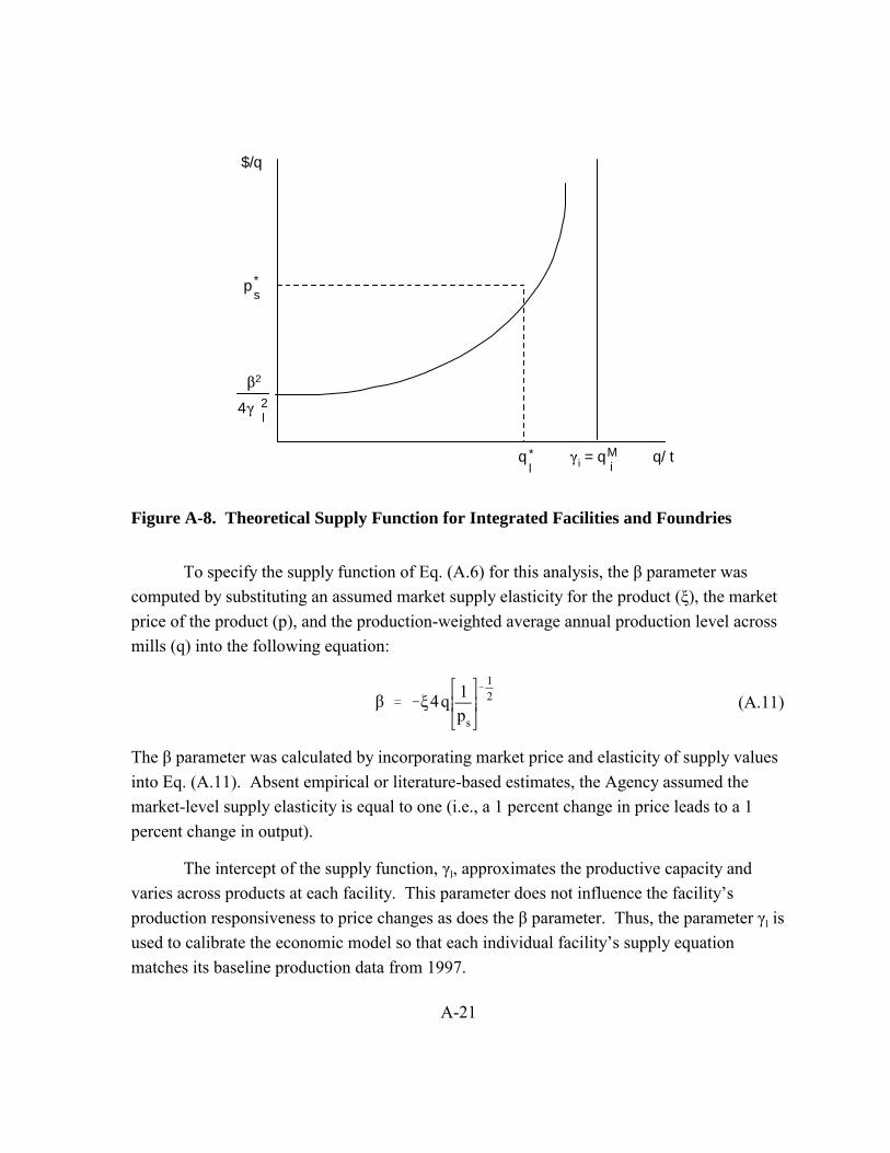
$/q

* ps

A2

4E 2 l

ql* Ei = qM q/ t

i

Figure A-8. Theoretical Supply Function for Integrated Facilities and Foundries

To specify the supply function of Eq. (A.6) for this analysis, the β parameter was computed by substituting an assumed market supply elasticity for the product (ξ), the market price of the product (p), and the production-weighted average annual production level across mills (q) into the following equation:

1

β � �ξ 4q 1 2 (A.11)ps

The β parameter was calculated by incorporating market price and elasticity of supply values into Eq. (A.11). Absent empirical or literature-based estimates, the Agency assumed the market-level supply elasticity is equal to one (i.e., a 1 percent change in price leads to a 1 percent change in output).

The intercept of the supply function, γl, approximates the productive capacity and varies across products at each facility. This parameter does not influence the facility’s production responsiveness to price changes as does the β parameter. Thus, the parameter γl is used to calibrate the economic model so that each individual facility’s supply equation matches its baseline production data from 1997.

A-21

Modeling the Impact of Compliance Costs. The effect of the regulation is to increase the MC of producing furnace coke by the compliance costs. These costs include the variable component consisting of the operating and maintenance costs and the nonvariable component consisting of the control equipment required for the regulatory option. Regulatory control costs will shift the supply curve upward for each affected facility by the annualized compliance cost (operating and maintenance plus annualized capital) expressed per unit of coke production. Computing the supply shift in this way treats compliance costs as the conceptual equivalent of a unit tax on output. For coke facilities, the horizontal portion of its supply curve will rise by the per-unit total compliance costs. In this case, the MC curve will shift by this amount to allow the new higher reservation price for the coke battery to appropriately reflect the fixed costs of compliance in the operating decision. At a multiple-battery facility, the change in each battery’s MC may cause a reordering of the steps because the compliance costs vary due to the technology, age, and existing controls of individual batteries.

Compliance costs on captive furnace coke batteries will directly affect production decisions at integrated mills, while compliance costs on merchant furnace coke batteries will indirectly affect these decisions through the change in the market price of furnace coke. Both of these impacts were modeled as reducing the net price integrated mills receive for finished steel products. Returning to the integrated mill’s supply function presented in Eq. (A.10), the mill’s production quantity with compliance costs is expressed as

where

q Ss β 1 I(l) � γl �

2 ps � r S (A.12) I(l) [ αl ∆cl � (1 � αl ) ∆pc ]

rI(sl) = the coke rate for integrated steel mill (l), which specifies the amount of

furnace coke input per unit of steel mill product;

αl = the share of integrated steel mill l’s furnace coke provided by captive batteries;

∆cl = change in per-unit cost of captive coke production at integrated steel mill l;

(1–αl) = share of integrated steel mill l’s furnace coke provided by the market; and

∆pc = change in the market price for furnace coke.

A-22

The bracketed term in the denominator represents the increased costs due to the regulation, i.e., both the direct and indirect effects. These costs, ∆cl and ∆pc, are expressed per ton of furnace coke and weighted to reflect each integrated mill’s reliance on captive versus market furnace coke.2 The change in the cost per ton of furnace coke due to the regulation is then multiplied by the mill’s coke rate to obtain the change in the cost per ton of finished steel product. The change in the cost per ton of finished steel product corresponds to the shift in the affected facility supply curve shown in Figure A-5b.

Supply from Nonintegrated Mills. The supply of steel mill products from domestic nonintegrated mills is specified as

NI � A s NI (A.13)q Ss NI (p s )ξ

s

where

A s NI = multiplicative parameter for nonintegrated mill supply equation, and

ξsNI = the nonintegrated mill supply elasticity for finished steel products (assumed

value = 1).

Absent literature or econometric estimates of the supply elasticity, this analysis employed an assumed value of one, which was then varied in conducting a sensitivity analysis for this parameter. The multiplicative supply parameter is determined by backsolving Eq. (A.8), given baseline values of the market price, supply elasticities, and quantities supplied by nonintegrated mills and foreign mills.

Foreign Supply (Imports). The supply of steel mill products from foreign suppliers (imports) is specified as

FqFSs

� AFs (p s )ξ

s (A.14)

2The captive versus market furnace coke weights are endogenous in the model because integrated mills exhaust their captive supply of coke first; hence, changes in coke consumption typically come from changes in market purchases, while captive consumption remains relatively constant.

A-23

where

AFs = multiplicative parameter for foreign supply equation, and

ξsF = the foreign supply elasticity for finished steel products (assumed value = 1).

Absent literature or econometric estimates (new or existing) of the supply elasticity, this analysis employed an assumed value of one, which was then varied in conducting a sensitivity analysis for this parameter. The multiplicative supply parameters are determined by backsolving Eq. (A.8), given baseline values of the market price, supply elasticity, and level of imports.

A.3.2.2 Market Demand for Steel Mill Products

The market demand for finished steel mill products, QDs, is the sum of domestic and foreign demand, i.e.,

Q Ds � q Ds

� qFDs (A.15)D

where

q Ds D = domestic demand for finished steel mill products, and

qFDs = foreign demand for steel mill products (exports).

Domestic Demand for Steel Mill Products. The domestic demand for finished steel products is expressed as

D D (A.16)q Ds

� BDs (p s )η

s

where

BDs = multiplicative parameter for domestic steel mill products demand equation,

and

ηs D = domestic demand elasticity for steel mill products (estimate = –0.59).

A-24

The multiplicative demand parameter calibrates the domestic demand equation given baseline data on price and demand elasticity to replicate the observed 1997 level of domestic consumption.

Foreign Demand for Steel Mill Products (Exports). Foreign demand (exports) for finished steel products is expressed as

FqFDs

� BFs (p s )η

s (A.17)

where

BFs = multiplicative demand parameter for foreign steel mill products’ demand

equation, and

ηs = foreign (export) demand elasticity for steel mill products (assumed value =F

–1).

The multiplicative demand parameter calibrates the foreign demand equation given data on price and demand elasticities to replicate the observed 1997 level of foreign exports.

A.3.3 Market for Foundry Coke

The market for furnace coke consists of supply from merchant coke plants and demand from foundries operating cupola furnaces. The domestic supply for foundry coke is modeled as a stepwise supply function developed from the marginal cost of production at individual foundry coke batteries. The domestic demand is derived from iron castings production at foundries operating cupola furnaces as determined through the market for iron castings and coking rates for individual batteries. As described previously, the level of imports and exports of foundry coke were negligible in 1997 and, thus, were not included in the market model. The following section details the market supply and demand components for this analysis.

A.3.3.1 Market Supply of Foundry Coke

The market supply of foundry coke, QSk, is composed solely of the supply from domestic merchant plants reflecting plant-level production decisions for individual merchant coke batteries, i.e.,

A-25

q Sk q SkQ Sk

� M Merchant

� ˆ ˆ M(l, j ) (A.18) l j

where

l = plants

j = batteries

q Sk M(l, j) = supply of foundry coke from coke battery (j) at merchant plant (l).

As was the case for furnace coke batteries, the marginal cost for an individual foundry coke battery is assumed to be constant reflecting a fixed-coefficient technology. Marginal cost curves were developed for all foundry coke batteries at merchant plants in the United States as detailed in Appendix B.

Foundry coke production decisions are based on the same approach used to model furnace coke production decisions. Thus, as illustrated previously in Figure A-7, the production decision is determined by an inverted L-shaped supply curve that is perfectly elastic to the capacity level of production and perfectly inelastic thereafter. Foundry coke batteries will supply 100 percent of capacity if its marginal cost is less than market price; otherwise, it will cease production. The regulatory costs shift each affected battery’s marginal cost upward, affecting facilities’ decision to operate or shut down individual batteries.

A.3.3.2 Market Demand for Foundry Coke

The market demand for foundry coke, QDk, is composed solely of the domestic demand by foundries operating cupola furnaces. Therefore, the foundry coke demand is derived from the production of iron castings from cupola furnaces. Increases in the price of foundry coke due to the regulation will lead to decreases in production of iron castings at foundries operating cupola furnaces. Foundries operating cupola furnaces are modeled as a single representative supplier. Thus, the demand function for foundry coke is expressed as follows:

Q Dk � q Dk

� r i CF (A.19)CF CF q Si

A-26

where

q Dk CF = derived demand for foundry coke from domestic cupola foundries;

r i CF = the coke rate for cupola foundries, which specifies the amount of foundry

coke input per unit output; and

q Si CF = quantity of iron castings produced at domestic cupola foundries;

Changes in production at foundries using electric arc and electric induction furnaces to produce iron castings do not affect the demand for foundry coke.

A.3.4 Market for Iron Castings

The market for iron castings consists of supply from domestic foundries and foreign imports and of demand from domestic and foreign consumers. Iron castings are modeled as a single commodity market. The domestic supply for iron castings includes production from foundries operating cupola furnaces that require foundry coke and from foundries that operate electric furnaces that do not. The proposed rule is expected to increase the price of foundry coke that will increase the cost of production at foundries with cupola furnaces and thereby shift their supply curves upward and increase the price of iron castings.

A.3.4.1 Market Supply of Iron Castings

The market supply for iron castings, QSi, is defined as the sum of the supply from domestic and foreign foundries. Domestic foundries are further segmented into operations using foundry coke (referred to as cupola foundries) and operations using electric furnaces (referred to as electric foundries). Supply is expressed as a function of the market price for castings:

Q Si � q Si

� q Si � qF

Si (A.20)CF EF

where

q Si CF = quantity of iron castings produced at domestic cupola foundries,

q Si EF = supply from domestic electric foundries, and

A-27

qFSi = supply from foreign foundries.

Domestic Cupola Foundries. The Agency used a simple supply function (Cobb Douglas) to characterize the production of iron castings. Compliance costs on captive foundry coke batteries will directly affect cupola foundries’ production decisions through the change in the market price of foundry coke. This impact is modeled as reducing the net revenue cupola foundries receive for the sales of iron castings. The aggregate cupola foundry’s supply function is expressed as

CF � A i CF ∆ p k )ξ

i

q Si CF (p i – r i CF (A.21)

where

A i CF = multiplicative supply parameter for cupola foundry’s supply equation,

r i CF = the coke rate for cupola foundries, which specifies the amount of foundry

coke input per unit output,

∆p k = change in the market price for foundry coke, and

ξiCF = supply elasticity for iron castings (assumed value = 1).

The multiplicative supply parameter, A i CF , is determined by backsolving Eq. (A.21), given

baseline values of the market price, supply elasticity, and quantity supplied.

Domestic Electric Furnace Foundries. The functional form of the supply curve for domestic foundries with electric arc or induction furnaces is specified as

EF � A i EF (A.22)q Si EF (p i )ξ

i

where

A i EF = multiplicative parameter for electric foundries supply equation, and

A-28

ξiEF = electric foundries supply elasticity for iron castings (assumed value = 1).

The multiplicative supply parameter, A i EF , is determined by backsolving Eq. (A.22), given

baseline values of the market price, supply elasticity, and quantity supplied from electric foundries.

Foreign Supply (Imports). The functional form of the foreign supply curve for iron castings is specified as

F (A.23)qFSi � AF

i (p i )ξi

where

AFi = multiplicative parameter for foreign iron castings supply equation, and

ξiF = foreign supply elasticity for iron castings (assumed value = 1).

The multiplicative supply parameter, AFi , is determined by backsolving Eq. (A.23), given

baseline values of the market price, supply elasticities, and level of imports.

A.3.4.2 Market Demand for Iron Castings

The market demand for iron castings (QDi) is the sum of domestic and foreign demand, and it is expressed as a function of the price of iron castings:

Q Di � q Di

� qFDi (A.24)D

where

q Di D = domestic demand for iron castings, and

qFDi = foreign demand (exports) for iron castings.

Domestic Demand for Iron Castings. The domestic demand for iron castings is expressed as

A-29

D D (A.25)q Di

� BDi (p i )η

i

where

B i D = multiplicative parameter for domestic iron castings’ demand equation, and

η i D = domestic demand elasticity for steel mill products (estimate = –0.58).

The domestic demand elasticity for iron casting products is expected to be inelastic and assumed to be –0.58. The multiplicative demand parameter calibrates the domestic demand equation given baseline data on price and demand elasticity to replicate the observed 1997 level of domestic consumption.

Foreign Demand for Iron Castings. Foreign demand (exports) for iron castings is expressed as

F (A.26)qFDi

� BFi (p i )η

i

where

BFi = multiplicative demand parameter for foreign steel mill products’ demand

equation, and

ηiF = foreign (export) demand elasticity for steel mill products (assumed value =

–1).

The foreign demand elasticity for iron casting products is assumed to be –1.0, which is more elastic than the domestic demand elasticity of –0.58. The multiplicative demand parameter calibrates the foreign demand equation given data on price and demand elasticities to replicate the observed 1997 level of foreign exports.

A.3.5 Post-regulatory Market Equilibrium Determination

Integrated steel mills and iron foundries with cupola furnaces must determine output given the market prices for their finished products, which in turn determines their furnace and

A-30

foundry coke requirements. The optimal output of finished steel products at integrated mills also depends on the cost of producing captive furnace coke and the market price of furnace coke; whereas iron foundries with cupolas depend on only the market price of foundry coke because they have no captive operations. Excess production of captive furnace coke at integrated mills will spill over into the furnace coke market; whereas an excess demand will cause the mill to demand furnace coke from the market. For merchant coke plants, the optimal market supply of furnace and/or foundry coke will be determined by the market price of each coke product.

Facility responses and market adjustments can be conceptualized as an interactive feedback process. Facilities face increased costs from the regulation, which initially reduce output. The cumulative effect of these individual changes leads to an increase in the market price that all producers (affected and unaffected) and consumers face, which leads to further responses by producers (affected and unaffected) as well as consumers and thus new market prices, and so on. The new equilibrium after imposing the regulation is the result of a series of iterations between producer and consumer responses and market adjustments until a stable market price arises where market supply equals market demand for each product, i.e., QS = QD.

The Agency employed a Walrasian auctioneer process to determine equilibrium price (and output) associated with the increased production costs of coke. The auctioneer calls out a market price for each product and evaluates the reactions by all participants (producers and consumers), comparing total quantities supplied and demanded to determine the next price that will guide the market closer to equilibrium (i.e., where market supply equals market demand). Decision rules are established to ensure that the process will converge to an equilibrium, in addition to specifying the conditions for equilibrium. The result of this approach is a vector of prices with the proposed regulation that equilibrates supply and demand for each product.

The algorithm for deriving the with-regulation equilibria in all markets can be generalized to five recursive steps:

1. Impose the control costs for each affected facility, thereby affecting their supply decisions.

2. Recalculate the production decisions for coke products and both final steel mill products and iron castings across all affected facilities. The adjusted production of steel mill products from integrated steel mills and iron castings from foundries

A-31

with cupola furnaces determines the derived demand for furnace and foundry coke through the input ratios. Therefore, the domestic demand for furnace and foundry coke is simultaneously determined with the domestic supply of final steel mill products and iron castings from these suppliers. After accounting for these adjustments, recalculate the market supply of all products by aggregating across all producers, affected and unaffected.

3. Determine the new prices via a price revision rule for all product markets.

4. Recalculate the supply functions of all facilities with the new prices, resulting in a new market supply of each product, in addition to derived (domestic) demand for furnace and foundry coke. Evaluate domestic demand for final steel mill products and iron castings, as well as import supply and export demand for appropriate products given the new prices.

5. Go to Step #3, resulting in new prices for each product. Repeat until equilibrium conditions are satisfied in all markets (i.e., the ratio of supply to demand is approximately one for each and every product).

A.3.6 Economic Welfare Impacts

The economic welfare implications of the market price and output changes with the regulation can be examined using two slightly different tactics, each giving a somewhat different insight but the same implications: changes in the net benefits of consumers and producers based on the price changes and changes in the total benefits and costs of these products based on the quantity changes. This analysis focuses on the first measure—the changes in the net benefits of consumers and producers. Figure A-9 depicts the change in economic welfare by first measuring the change in consumer surplus and then the change in producer surplus. In essence, the demand and supply curves previously used as predictive devices are now being used as a valuation tool.

This method of estimating the change in economic welfare with the regulation divides society into consumers and producers. In a market environment, consumers and producers of the good or service derive welfare from a market transaction. The difference between the maximum price consumers are willing to pay for a good and the price they actually pay is referred to as “consumer surplus.” Consumer surplus is measured as the area under the demand curve and above the price of the product. Similarly, the difference between the minimum price producers are willing to accept for a good and the price they actually receive is referred to as “producer surplus” or profits. Producer surplus is measured as the area above the supply curve and below the price of the product. These areas can be thought of as

A-32

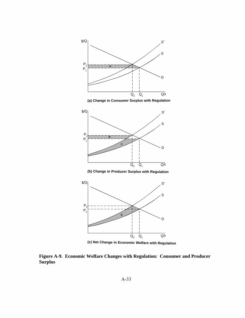
$/Q

P2 P1

S�

A

S

D

Q/tQ2 Q1

(a) Change in Consumer Surplus with Regulation

$/Q

P2 P1

B

C

S

S�

D

Q2 Q1 Q/t

(b) Change in Producer Surplus with Regulation

$/Q

P2 P1

D

S

S�

D

Q2 Q1 Q/t

(c) Net Change in Economic Welfare with Regulation

Figure A-9. Economic Welfare Changes with Regulation: Consumer and Producer Surplus

A-33

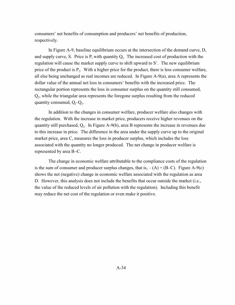
consumers’ net benefits of consumption and producers’ net benefits of production, respectively.

In Figure A-9, baseline equilibrium occurs at the intersection of the demand curve, D, and supply curve, S. Price is Pl with quantity Ql. The increased cost of production with the regulation will cause the market supply curve to shift upward to Sk. The new equilibrium price of the product is P2. With a higher price for the product, there is less consumer welfare, all else being unchanged as real incomes are reduced. In Figure A-9(a), area A represents the dollar value of the annual net loss in consumers’ benefits with the increased price. The rectangular portion represents the loss in consumer surplus on the quantity still consumed, Q2, while the triangular area represents the foregone surplus resulting from the reduced quantity consumed, Ql–Q2.

In addition to the changes in consumer welfare, producer welfare also changes with the regulation. With the increase in market price, producers receive higher revenues on the quantity still purchased, Q2. In Figure A-9(b), area B represents the increase in revenues due to this increase in price. The difference in the area under the supply curve up to the original market price, area C, measures the loss in producer surplus, which includes the loss associated with the quantity no longer produced. The net change in producer welfare is represented by area B–C.

The change in economic welfare attributable to the compliance costs of the regulation is the sum of consumer and producer surplus changes, that is, – (A) + (B–C). Figure A-9(c) shows the net (negative) change in economic welfare associated with the regulation as area D. However, this analysis does not include the benefits that occur outside the market (i.e., the value of the reduced levels of air pollution with the regulation). Including this benefit may reduce the net cost of the regulation or even make it positive.

A-34

APPENDIX B

DEVELOPMENT OF COKE BATTERY COST FUNCTIONS

This appendix outlines EPA’s method for estimating 1997 baseline production costs for coke batteries. The Agency used a coke production cost model developed in support of the 1993 MACT on coke ovens. EPA’s Technical Approach for a Coke Production Cost Model (EPA, 1979) provides a more detailed description of this model. For this analysis, the model was updated with reported technical characteristics of coke batteries from the Information Collection Request (ICR) survey responses and available price data. In addition, the Agency incorporated estimates of MACT pollution abatement costs developed for the 1993 MACT on coke ovens (EPA, 1991).

B.1 Variable Costs

Coke batteries use four variable inputs during the manufacturing process— metallurgical coal, labor, energy, and other materials/supplies. Metallurgical coal is essentially the only raw material used in the production of coke. Labor transports and delivers the raw materials as well as final products. Coke ovens and auxiliary equipment consume energy and supplies during the production process and periodic maintenance and repair of the coke batteries.

Coke production requires a fixed amount of each variable input per ton of coke, and these inputs are not substitutable. Accordingly, the total variable cost function is linear in the output and input prices, or, in other words, the average variable cost function is independent of output. Therefore, the average variable cost function (expressed in dollars per short ton of coke) can be written as

AVC = AV_CI`Pc + AV_LI`w + AV_EI`Pe + AV_OI`Po (B.1)

where AV_CI, AV_LI, AV_EI, and AV_OI are the fixed requirements per ton of coke of metallurgical coal, labor, energy, and other material and supplies. Pc, w, Pe, and Po are the prices of each variable input, respectively. As shown above, the contribution of each variable input to the per-unit coke cost is equal to the average variable input (fixed requirement of the input per ton of coke) times the price of the input. For example, the contribution of labor to

B-1

the cost per ton of coke (AV_LI) is equal to the labor requirement per ton of coke times the price of labor (w).

The variable costs above include those costs associated with by- and co-product recovery operations associated with the coke battery. To more accurately reflect the costs specific to coke production, the Agency subtracted by- and co-product revenues/credits from Eq. (B.1). By-products include tar and coke oven gas among others, while co-products include coke breeze and other industrial coke. Following the same fixed coefficient approach, these revenues or credits (expressed per ton of coke) are derived for each recovered product at the coke battery by multiplying the appropriate yield (recovered product per ton of coke) by its price or value. The variable cost components and by-/co-product credits are identified below.

B.1.1 Metallurgical Coal (AVCI, Pc)

The ICR survey responses provided the fixed input requirement for metallurgical coal at each battery. Based on the responses from the survey, U.S. coke producers require an average of 1.36 tons of coal per ton of coke produced. This fixed input varies by type of producer. Integrated, or captive, producers require an average of 1.38 tons of coal per ton of coke produced, while merchant producers require an average of 1.31 tons of coal per ton of coke produced. The U.S. Department of Energy (1998) provides state-level coal price data for metallurgical coal. For each coke battery, EPA computed the cost of coal per short ton of coke by multiplying its input ratio times the appropriate state or regional price. As shown in Table B-1, the average cost of metallurgical coal per ton of coke in 1997 was $66.27 for captive producers and $63.77 for merchant producers.

B.1.2 Labor (AVLI, w)

The cost model provides an estimate of the fixed labor requirement for operation, maintenance, and supervision labor at each battery. The Agency used these estimates to derive the average variable labor cost for each individual battery given its technical characteristics and the appropriate state-level wage rates obtained from the U.S. Bureau of Labor Statistics (1998). As shown in Table B-2, average labor costs per ton of coke are significantly lower for captive producers (e.g., $15.74 per ton of coke) relative to merchant producers (e.g., $27.21 per ton of coke). Captive batteries are typically larger capacity batteries and therefore require fewer person-hours per ton of coke.

B-2

Table B-1. Metallurgical Coal Costs by Producter Type: 1997 ($/ton of coke)

Captive Merchant All Coke Batteries Number of batteries 40 18 58 Average $66.27 $63.77 $65.49 Minimum $59.25 $56.18 $56.18 Maximum $77.56 $70.34 $77.56

Table B-2. Labor Costs by Producer Type: 1997 ($/ton of coke)

Captive Merchant All Coke Batteries Number of batteries 40 18 58

Average $15.74 $27.21 $19.30

Minimum $8.62 $10.48 $8.62

Maximum $31.04 $42.04 $42.04

B.1.3 Energy (AVEI, Pe)

The cost model estimates the fixed energy requirements (i.e., electricity, steam, and water) for each battery. These estimates are used to derive the energy costs per ton of coke for each battery. Captive producers have a lower electricity requirement (i.e., 47.58 kWh per ton of coke) relative to merchant producers (i.e., 50.96 kWh per ton of coke). As shown in Table B-3, the average energy cost per ton of coke across all coke batteries is $4.36. Average energy costs per ton of coke are lower for captive producers (e.g., $4.19 per ton of coke) relative to merchant producers (e.g., $4.71 per ton of coke). This difference reflects lower state/regional electricity prices in regions where captive batteries produce coke.

B-3

Table B-3. Energy Costs by Producer Type: 1997 ($/ton of coke)

Captive Merchant All Coke Batteries Number of batteries 40 18 58

Average $4.19 $4.71 $4.36

Minimum $3.00 $3.13 $3.00

Maximum $10.59 $10.59 $10.59

B.1.4 Other Materials and Supplies (AVOI, Po)

The fixed requirements for other materials and supplies associated with the production of coke include

` chemicals,

` maintenance materials,

` safety and clothing, and

` laboratory and miscellaneous supplies.

As shown in Table B-4, the cost model estimates the average cost for these items across all coke batteries is $4.02 per short ton of coke, ranging from $2.73 to $6.56 per ton of coke. These costs vary by producer type, with merchant producers averaging $4.82 per ton of coke versus captive producers who average $3.66 per ton of coke.

B.1.5 By- and Co-product Credits

In addition to the variable cost inputs described above, by- and co-products are associated with the manufacture of coke products. Therefore, the Agency modified Eq. (B.1) by subtracting (1) revenues generated from the sale of by-/co-products and (2) credits associated with using of coke oven gas as an energy input in the production process. The following cost function adjustments were made to the engineering model to incorporate by-and co-products into the cokemaking cost function:

B-4

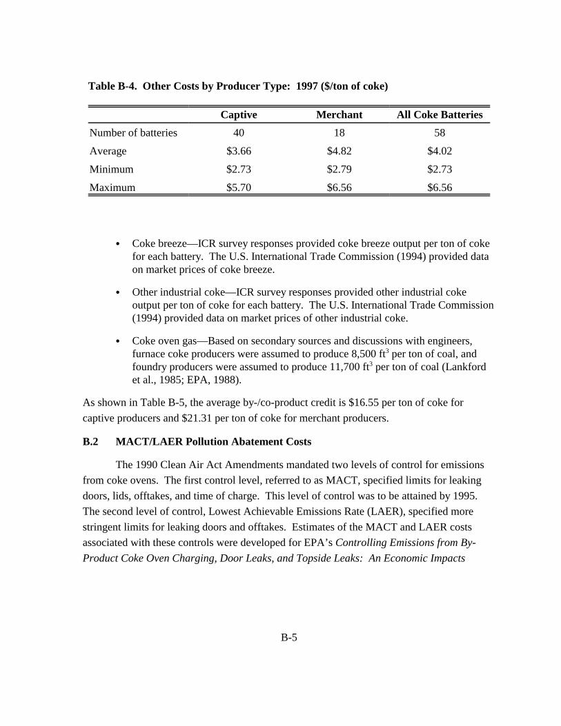
Table B-4. Other Costs by Producer Type: 1997 ($/ton of coke)

Captive Merchant All Coke Batteries Number of batteries 40 18 58

Average $3.66 $4.82 $4.02

Minimum $2.73 $2.79 $2.73

Maximum $5.70 $6.56 $6.56

` Coke breeze—ICR survey responses provided coke breeze output per ton of coke for each battery. The U.S. International Trade Commission (1994) provided data on market prices of coke breeze.

` Other industrial coke—ICR survey responses provided other industrial coke output per ton of coke for each battery. The U.S. International Trade Commission (1994) provided data on market prices of other industrial coke.

` Coke oven gas—Based on secondary sources and discussions with engineers, furnace coke producers were assumed to produce 8,500 ft3 per ton of coal, and foundry producers were assumed to produce 11,700 ft3 per ton of coal (Lankford et al., 1985; EPA, 1988).

As shown in Table B-5, the average by-/co-product credit is $16.55 per ton of coke for captive producers and $21.31 per ton of coke for merchant producers.

B.2 MACT/LAER Pollution Abatement Costs

The 1990 Clean Air Act Amendments mandated two levels of control for emissions from coke ovens. The first control level, referred to as MACT, specified limits for leaking doors, lids, offtakes, and time of charge. This level of control was to be attained by 1995. The second level of control, Lowest Achievable Emissions Rate (LAER), specified more stringent limits for leaking doors and offtakes. Estimates of the MACT and LAER costs associated with these controls were developed for EPA’s Controlling Emissions from By-Product Coke Oven Charging, Door Leaks, and Topside Leaks: An Economic Impacts

B-5

Table B-5. By-/Co-Product Credits by Producer Type: 1997 ($/ton of coke)

Captive Merchant All Coke Batteries Number of batteries 40 18 58

Average $16.55 $21.31 $18.03

Minimum $13.41 $8.83 $8.83

Maximum $30.95 $48.30 $48.30

Analysis (EPA, 1991).1 Table B-6 provides summary statistics for the projected costs associated with each level of control. However, the Agency determined that industry actions undertaken in the interim period to comply with the MACT limits have enabled them to also meet the LAER limits. Therefore, only the MACT-related pollution abatement costs have been incorporated to determine the appropriate baseline costs for the 1997 economic model. As shown in Table B-6, the average MACT pollution abatement cost across all coke batteries is $1.27 per short ton of coke. The projected costs for captive producers range from zero to $2.54 per ton of coke, while projected costs for merchant producers range from zero to $10.93 per ton of coke.

B.3 Fixed Costs

Production of coke requires the combination of variable inputs outlined above with fixed capital equipment (e.g., coke ovens and auxiliary equipment). It also includes other overhead and administrative expenses. For each coke battery, the average fixed costs per ton of coke can be obtained by dividing the total fixed costs (TFC) estimated by the coke model by total battery coke production. Therefore, the average fixed cost function (expressed in dollars per ton of coke) can be written as

AFC = (PTI + ASE +PYOH+ PLOH)/Q (B.2)

1The Agency estimated costs for the LAER control level using two scenarios. The first (LAER-MIN) assumed all batteries will require new doors and jambs. The second (LAER-MAX) also assumed all batteries will require new doors and jambs and in addition assumed batteries with the most serious door leak problems would be rebuilt. This analysis reports cost estimates for the LAER-MIN scenario.

B-6

Table B-6. Pollution Abatement Costs by Producer Type: 1997 ($/ton of coke)

Captive Merchant All Coke Batteries Number of batteries MACT

Average Minimum Maximum

LAER Average Minimum Maximum

40 18 58

$0.82 $2.29 $1.27 $0.00 $0.00 $0.00 $2.54 $10.93 $10.93

$1.64 $2.44 $1.88 $0.07 $0.94 $0.07 $2.63 $6.07 $6.07

where

` property taxes and insurance (PTI) = (0.02)`($225`Coke Capacity). This category accounts for the fixed costs associated with property taxes and insurance for the battery. The cost model estimates this component as 2 percent of capital cost. Capital costs are estimated to be $225 per annual short ton of capacity based on reported estimates of capital investment cost of a rebuilt by-product coke-making facility (USITC, 1994). As shown in Table B-7, the average PTI cost across all batteries is $4.47 per ton of coke.

` administration and sales expense (ASE) = (0.02)`($225`Coke capacity). This category accounts for the fixed costs associated with administrative and sales expenses for the coke battery. The cost model also calculates this component as 2 percent of capital cost. As shown in Table B-7, the average cost across all coke batteries for ASE is $5.02 per ton of coke.

` payroll overhead (PYOH) = (0.2)`(Total labor costs). Payroll overhead is modified as 20 percent of total labor costs. Payroll overhead is used to capture fringe benefits because wage rates obtained from the Bureau of Labor Statistics exclude fringe benefits. As shown in Table B-7, the average payroll overhead is $3.15 per ton of coke for captive producers and $5.44 per ton of coke for merchant producers, reflecting the different labor requirements by producer type.

` plant overhead (PLOH) = (0.5)`(Total payroll + Total other expenses). The cost model computes plant overhead as 50 percent of total payroll and total other

B-7

Table B-7. Average Fixed Costs by Producer Type: 1997 ($/ton of coke)

Captive Merchant All Coke Batteries Number of batteries Property taxes and insurance

Average Minimum Maximum

Administrative and sales expense

Average Minimum Maximum

Payroll overhead Average Minimum Maximum

Plant overhead Average Minimum Maximum

40 18 58

$4.41 $4.58 $4.47 $3.20 $3.55 $3.20 $6.78 $6.11 $6.78

$4.96 $5.16 $5.02 $3.60 $4.00 $3.60 $7.63 $6.87 $7.63

$3.15 $5.44 $3.86 $1.72 $2.10 $1.72 $6.21 $8.41 $8.41

$9.33 $17.77 $11.95 $5.38 $7.50 $5.38

$17.67 $26.95 $26.95

expenses by producer type. As shown in Table B-7, the average plant overhead cost is $9.33 for captive producers and $17.77 for merchant producers. As with payroll overhead, this difference reflects differences in labor requirements for captive and merchant producers.

B.5 Summary of Results

Table B-8 summarizes each cost component and aggregates them to estimate the average total costs per ton of coke by producer type. As shown, the average total cost (ATC) across all coke batteries is $101.72 per short ton of coke. The ATC for captive producers is $95.99 per short ton of coke and is significantly lower than the ATC for merchant producers at $114.47. This difference reflects both economies of scale and lower production costs associated with the production of furnace coke. These differences are also consistent with

B-8

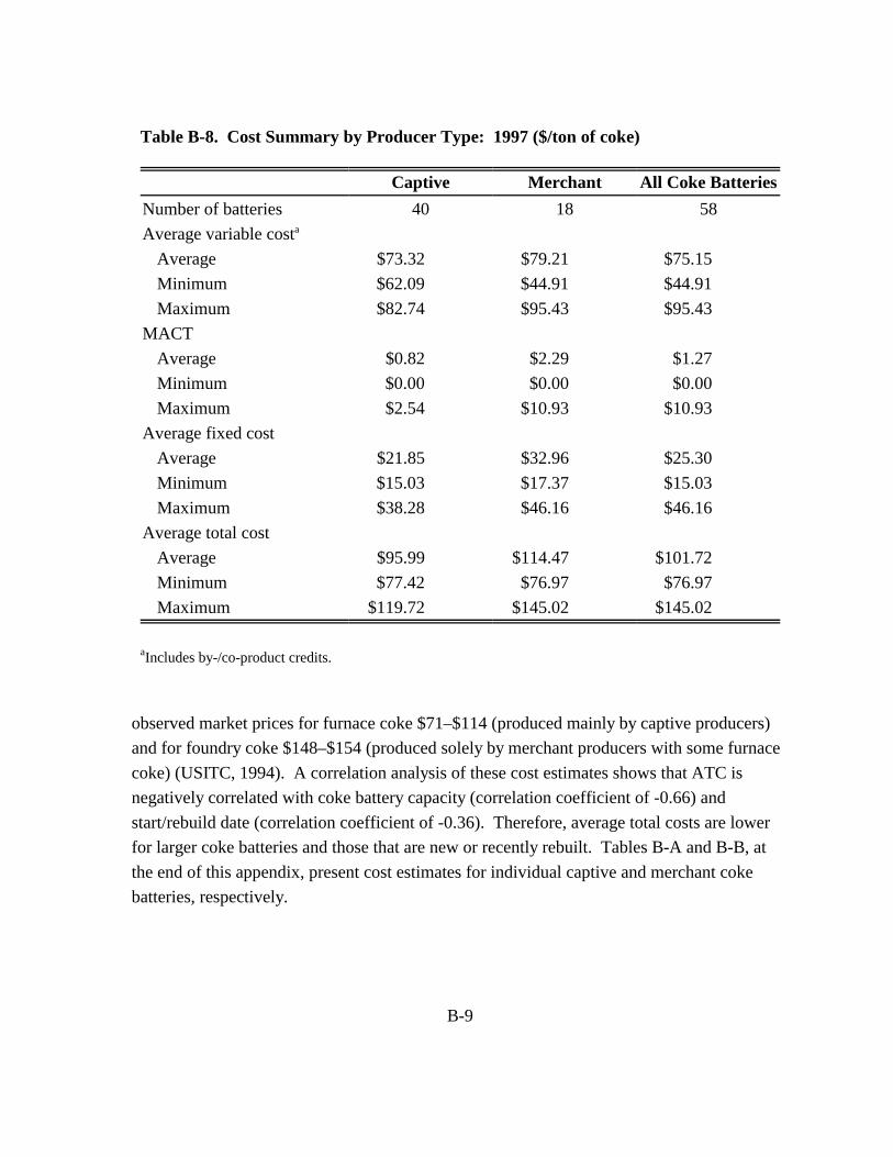
Table B-8. Cost Summary by Producer Type: 1997 ($/ton of coke)

Captive Merchant All Coke Batteries Number of batteries Average variable costa

Average Minimum Maximum

MACT Average Minimum Maximum

Average fixed cost Average Minimum Maximum

Average total cost Average Minimum Maximum

40 18 58

$73.32 $79.21 $75.15 $62.09 $44.91 $44.91 $82.74 $95.43 $95.43

$0.82 $2.29 $1.27 $0.00 $0.00 $0.00 $2.54 $10.93 $10.93

$21.85 $32.96 $25.30 $15.03 $17.37 $15.03 $38.28 $46.16 $46.16

$95.99 $114.47 $101.72 $77.42 $76.97 $76.97

$119.72 $145.02 $145.02

aIncludes by-/co-product credits.

observed market prices for furnace coke $71–$114 (produced mainly by captive producers) and for foundry coke $148–$154 (produced solely by merchant producers with some furnace coke) (USITC, 1994). A correlation analysis of these cost estimates shows that ATC is negatively correlated with coke battery capacity (correlation coefficient of -0.66) and start/rebuild date (correlation coefficient of -0.36). Therefore, average total costs are lower for larger coke batteries and those that are new or recently rebuilt. Tables B-A and B-B, at the end of this appendix, present cost estimates for individual captive and merchant coke batteries, respectively.

B-9

B.6 Nonrecovery Cokemaking

Several substitute technologies for by-product cokemaking have been developed in the United States and abroad. In the United States, the nonrecovery method is the only substitute that has a significant share of the coke market. This technology is relatively new, and, as a result, the original coke production cost model did not include estimates for these types of coke-making batteries. The nonrecovery process is less costly than the by-product process because of the absence of recovery operations and a lower labor input requirement per ton of coke. Therefore, the Agency modified the model to reflect these cost advantages in the following manner:

` No expenses/credits associated with by- and co-product recovery.

` Reduced labor input—labor requirement estimates generated by the model were multiplied by a factor of 0.11, which represents the ratio of employment per ton of coke at merchant batteries to employment per ton of coke at nonrecovery batteries.

` Exceed current standards of pollution abatement (Engineering and Mining Journal, 1997)—MACT compliance costs were excluded.

As shown in Table B-9, the ATC for nonrecovery coke-making facilities is $71.28 per ton of coke, which is significantly lower than the average ATC of captive and merchant producers. These costs vary slightly across these batteries ranging from $68.49 to $72.88 per ton of coke. Table B-C, at the end of this appendix, presents cost estimates for individual nonrecovery cokemaking batteries.

B-10

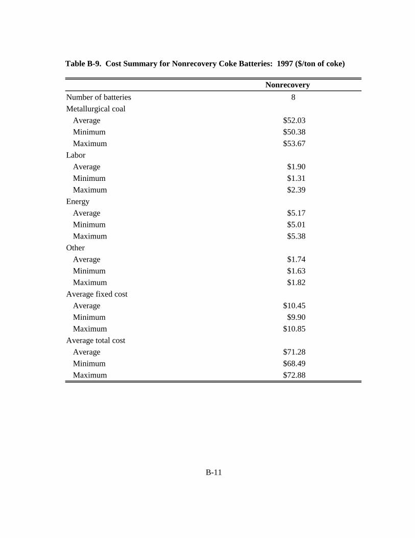
Table B-9. Cost Summary for Nonrecovery Coke Batteries: 1997 ($/ton of coke)

Nonrecovery Number of batteries Metallurgical coal

Average Minimum Maximum

Labor Average Minimum Maximum

Energy Average Minimum Maximum

Other Average Minimum Maximum

Average fixed cost Average Minimum Maximum

Average total cost Average Minimum Maximum

8

$52.03 $50.38 $53.67

$1.90 $1.31 $2.39

$5.17 $5.01 $5.38

$1.74 $1.63 $1.82

$10.45 $9.90

$10.85

$71.28 $68.49 $72.88

B-11

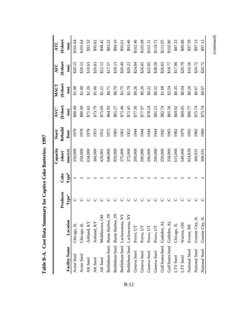
Tabl

e B-

A.

Cos

t Dat

a Su

mm

ary

for

Cap

tive

Cok

e Ba

tteri

es:

1997

Cap

acity

St

art/

AV

Cc

MA

CT

A

FC

AT

C

Prod

ucer

C

oke

(sho

rt

Reb

uild

($

/shor

t ($

/shor

t ($

/shor

t ($

/shor

t Fa

cilit

y N

ame

Loca

tion

Typ

ea T

ypeb

tons

/yr)

D

ate

ton)

to

n)

ton)

to

n)

Acm

e St

eel

Chi

cago

, IL

C

1 25

0,00

0 19

79

$80.

49

$1.0

0 $2

0.15

$1

01.6

4 A

cme

Stee

l C

hica

go, I

L C

1

250,

000

1978

$8

0.49

$1

.00

$20.

15

$101

.64

AK

Ste

el

Ash

land

, KY

C

1

634,

000

1978

$7

1.63

$1

.26

$18.

63

$91.

52

AK

Ste

el

Ash

land

, KY

C

1

366,

000

1953

$7

3.79

$1

.00

$20.

83

$95.

62

AK

Ste

el

Mid

dlet

own,

OH

C

1

429,

901

1952

$7

5.09

$1

.21

$22.

12

$98.

42

Bet

hleh

em S

teel

B

urns

Har

bor,

IN

C

1 94

8,00

0 19

72

$64.

93

$0.7

1 $1

7.57

$8

3.22

B

ethl

ehem

Ste

el

Bur

ns H

arbo

r, IN

C

1

929,

000

1983

$6

5.27

$0

.70

$18.

13

$84.

10

Bet

hleh

em S

teel

La

ckaw

anna

, NY

C

1

375,

000

1962

$7

1.46

$1

.75

$20.

40

$93.

61

Bet

hleh

em S

teel

La

ckaw

anna

, NY

C

1

375,

000

1952

$7

1.45

$1

.79

$20.

22

$93.

46

Gen

eva

Stee

l Pr

ovo,

UT

C

1 20

0,00

0 19

44

$77.

36

$0.2

6 $2

4.84

$1

02.4

6 G

enev

a St

eel

Prov

o, U

T C

1

200,

000

1944

$7

7.97

$0

.26

$26.

85

$105

.08

Gen

eva

Stee

l Pr

ovo,

UT

C

1 20

0,00

0 19

44

$78.

24

$0.2

2 $2

2.85

$1

01.3

1 G

enev

a St

eel

Prov

o, U

T C

1

200,

000

1944

$8

1.21

$0

.22

$38.

28

$119

.72

Gul

f Sta

tes S

teel

G

adsd

en, A

L C

1

250,

000

1942

$8

2.74

$1

.68

$26.

63

$111

.05

Gul

f Sta

tes S

teel

G

adsd

en, A

L C

1

250,

000

1965

$8

1.56

$2

.54

$18.

77

$102

.86

LTV

Ste

el

Chi

cago

, IL

C

1 61

5,00

0 19

82

$69.

02

$0.3

5 $1

7.96

$8

7.33

LT

V S

teel

W

arre

n, O

H

C

1 54

9,00

0 19

79

$69.

05

$0.0

4 $2

0.79

$8

9.88

N

atio

nal S

teel

Ec

orse

, MI

C

1 92

4,83

9 19

92

$80.

77

$0.2

6 $1

6.56

$9

7.59

N

atio

nal S

teel

G

rani

te C

ity, I

L C

1

300,

931

1982

$7

5.74

$0

.67

$20.

72

$97.

13

Nat

iona

l Ste

el

Gra

nite

City

, IL

C

1 30

0,93

1 19

80

$75.

74

$0.6

7 $2

0.72

$9

7.13

(con

tinue

d)

B-12

Tabl

e B-

A.

Cos

t Dat

a Su

mm

ary

for

Cap

tive

Cok

e Ba

tteri

es:

1997

(con

tinue

d)

Cap

acity

St

art/

AV

Cc

MA

CT

A

FC

AT

C

Prod

ucer

C

oke

(sho

rt

Reb

uild

($

/shor

t ($

/shor

t ($

/shor

t ($

/shor

t Fa

cilit

y N

ame

Loca

tion

Typ

ea T

ypeb

tons

/yr)

D

ate

ton)

to

n)

ton)

to

n)

USX

C

lairt

on, P

A

C

1 84

4,61

0 19

82

$64.

94

$0.7

1 $1

5.28

$8

0.92

U

SX

Cla

irton

, PA

C

1

668,

680

1976

$6

5.89

$0

.00

$19.

72

$85.

61

USX

C

lairt

on, P

A

C

1 66

8,68

0 19

78

$65.

89

$0.0

0 $1

9.72

$8

5.61

U

SX

Cla

irton

, PA

C

1

373,

395

1989

$6

8.36

$0

.00

$20.

96

$89.

32

USX

C

lairt

on, P

A

C

1 37

3,39

5 19

89

$68.

36

$0.0

0 $2

0.96

$8

9.32

U

SX

Cla

irton

, PA

C

1

373,

395

1979

$6

8.36

$1

.02

$20.

96

$90.

34

USX

C

lairt

on, P

A

C

1 37

8,50

5 19

55

$70.

52

$1.0

2 $2

1.96

$9

3.50

U

SX

Cla

irton

, PA

C

1

378,

505

1955

$7

0.52

$1

.07

$21.

96

$93.

55

USX

C

lairt

on, P

A

C

1 37

8,50

5 19

55

$70.

52

$1.0

7 $2

1.96

$9

3.55

U

SX

Cla

irton

, PA

C

1

378,

505

1954

$7

1.75

$1

.07

$21.

69

$94.

51

USX

C

lairt

on, P

A

C

1 37

8,50

5 19

54

$71.

75

$1.0

2 $2

1.69

$9

4.46

U

SX

Cla

irton

, PA

C

1

378,

505

1954

$7

1.75

$0

.00

$21.

69

$93.

44

USX

G

ary,

IN

C

1 82

7,82

0 19

76

$73.

33

$0.6

4 $2

2.55

$9

6.52

U

SX

Gar

y, IN

C

1

827,

820

1975

$7

4.13

$0

.64

$21.

93

$96.

70

USX

G

ary,

IN

C

1 29

7,11

0 19

54

$79.

40

$1.4

8 $2

3.84

$1

04.7

2 U

SX

Gar

y, IN

C

1

297,

110

1954

$7

9.68

$1

.48

$24.

98

$106

.14

Whe

elin

g-Pi

tt Fo

llans

bee,

WV

C

1

782,

000

1977

$6

2.09

$0

.30

$15.

03

$77.

42

Whe

elin

g-Pi

tt Fo

llans

bee,

WV

C

1

163,

000

1964

$7

6.53

$1

.33

$28.

51

$106

.37

Whe

elin

g-Pi

tt Fo

llans

bee,

WV

C

1

151,

000

1955

$7

7.49

$1

.09

$27.

79

$106

.37

Whe

elin

g-Pi

tt Fo

llans

bee,

WV

C

1

151,

000

1953

$7

7.49

$1

.09

$27.

79

$106

.38

a C =

Cap

tive;

M =

Mer

chan

t. b 1

= Fu

rnac

e; 2

= F

ound

ry; 3

= B

oth.

B-13

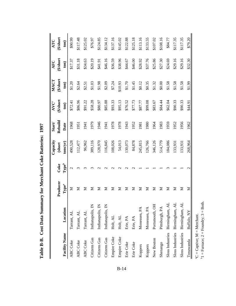
Tabl

e B-

B. C

ost D

ata

Sum

mar

y fo

r M

erch

ant C

oke

Batte

ries

: 19

97

Cap

acity

St

art/

AV

Cc

MA

CT

A

FC

AT

C

Prod

ucer

C

oke

(sho

rt

Reb

uild

($

/shor

t ($

/shor

t ($

/shor

t ($

/shor

t Fa

cilit

y N

ame

Loca

tion

Typ

ea T

ypeb

tons

/yr)

D

ate

ton)

to

n)

ton)

to

n)

AB

C C

oke

Tarr

ant,

AL

M

2 49

0,52

8 19

68

$72.

41

$1.2

0 $1

7.37

$9

0.99

AB

C C

oke

Tarr

ant,

AL

M

3 11

2,47

7 19

51

$86.

96

$2.6

4 $3

1.18

$1

17.4

8

AB

C C

oke

Tarr

ant,

AL

M

3 96

,962

19

41

$91.

22

$2.5

1 $3

4.63

$1

25.0

2

Citi

zens

Gas

In

dian

apol

is, I

N

M

3 38

9,11

6 19

79

$58.

28

$1.0

3 $2

0.19

$7

6.97

Citi

zens

Gas

In

dian

apol

is, I

N

M

2 12

8,97

0 19

46

$80.

97

$1.9

8 $4

1.91

$1

24.8

5

Citi

zens

Gas

In

dian

apol

is, I

N

M

2 11

6,84

5 19

41

$85.

88

$2.0

9 $4

6.16

$1

34.1

2

Empi

re C

oke

Hol

t, A

L M

2

108,

026

1978

$9

3.33

$7

.24

$36.

59

$137

.16

Empi

re C

oke

Hol

t, A

L M

2

54,0

13

1978

$9

5.13

$1

0.93

$3

8.96

$1

45.0

2

Erie

Cok

e Er

ie, P

A

M

2 13

0,07

3 19

43

$76.

52

$1.7

0 $4

4.67

$1

22.8

8

Erie

Cok

e Er

ie, P

A

M

2 84

,878

19

52

$77.

73

$1.4

5 $4

6.00

$1

25.1

8

Kop

pers

M

ones

sen,

PA

M

1

245,

815

1981

$8

7.77

$0

.12

$28.

92

$113

.16

Kop

pers

M

ones

sen,

PA

M

1

126,

766

1980

$9

9.08

$0

.35

$37.

76

$133

.55

New

Bos

ton

Ports

mou

th, O

H

M

1 34

6,12

6 19

64

$83.

67

$1.3

2 $2

5.86

$1

07.0

2

Shen

ango

Pi

ttsbu

rgh,

PA

M

1

514,

779

1983

$8

4.44

$0

.00

$27.

30

$108

.16

Slos

s Ind

ustri

es

Birm

ingh

am, A

L M

3

184,

086

1959

$6

2.04

$1

.58

$24.

69

$84.

77

Slos

s Ind

ustri

es

Birm

ingh

am, A

L M

1

133,

931

1952

$9

0.33

$1

.58

$29.

16

$117

.35

Slos

s Ind

ustri

es

Birm

ingh

am, A

L M

1

133,

931

1956

$9

0.33

$1

.58

$29.

16

$117

.35

Tona

wan

da

Buf

falo

, NY

M

2

268,

964

1962

$4

4.91

$1

.99

$32.

30

$79.

20

a C =

Cap

tive;

M =

Mer

chan

t. b 1

= Fu

rnac

e; 2

= F

ound

ry; 3

= B

oth.

B-14

Tabl

e B-

C.

Cos

t Dat

a Su

mm

ary

for

Non

reco

very

Cok

e Ba

tteri

es:

1997

Cap

acity

St

art/

AV

Cc

MA

CT

A

FC

AT

C

Prod

ucer

C

oke

(sho

rt

Reb

uild

($

/shor

t ($

/shor

t ($

/shor

t ($

/shor

t Fa

cilit

y N

ame

Loca

tion

Typ

ea T

ypeb

tons

/yr)

D

ate

ton)

to

n)

ton)

to

n)

Jew

ell C

oke

Van

sant

, VA

M

1

197,

000

1966

$5

8.59

$0

.00

$9.9

0 $6

8.49

an

d C

oal

Jew

ell C

oke

Van

sant

, VA

M

1

164,

000

1983

$5

9.31

$0

.00

$10.

38

$69.

69

and

Coa

l

Jew

ell C

oke

Van

sant

, VA

M

1

124,

000

1989

$5

9.98

$0

.00

$10.

85

$70.

83

and

Coa

l

Jew

ell C

oke

Van

sant

, VA

M

1

164,

000

1990

$5

9.31

$0

.00

$10.

38

$69.

69

and

Coa

l

Indi

ana

Har

bor

East

Chi

cago

, IN

M

1

325,

000

1998

$6

2.36

$0

.00

$10.

52

$72.

88

Cok

e C

o

Indi

ana

Har

bor

East

Chi

cago

, IN

M

1

325,

000

1998

$6

2.36

$0

.00

$10.

52

$72.

88

Cok

e C

o

Indi

ana

Har

bor

East

Chi

cago

, IN

M

1

325,

000

1998

$6

2.36

$0

.00

$10.

52

$72.

88

Cok

e C

o

Indi

ana

Har

bor

East

Chi

cago

, IN

M

1

325,

000

1998

$6

2.36

$0

.00

$10.

52

$72.

88

Cok

e C

o

a C =

Cap

tive;

M =

Mer

chan

t. b 1

= Fu

rnac

e; 2

= F

ound

ry; 3

= B

oth.

c In

clud

es b

y-/c

o-pr

oduc

t cre

dits

.

B-15

APPENDIX C

ECONOMETRIC ESTIMATION OF THE DEMAND ELASTICITY FOR STEEL MILL PRODUCTS

This appendix summarizes EPA’s estimation of the demand elasticities for steel mill products. These estimates are based on national-level data from 1987 through 1997 as obtained from the AISI (1990, 1992, 1997), U.S. Bureau of the Census (1988-1998, 1997, 1998), U.S. Bureau of Labor Statistics (1998), and other government sources (U.S. Department of Energy, 1990, 1998 and U.S. Geological Survey 1987-1990, 1995-1997). The following sections summarize the econometric procedure and present the estimates of the demand elasticity for the following nine steel mill products:

` semi-finished products

` structural shapes and plates

` rails and track accessories

` bars

` tool steel

` pipe and tubing

` wire

` tin mill

` sheet and strip

C.1 Econometric Model

A partial equilibrium market supply/demand model is specified as a system of interdependent equations in which the price and output of a product are simultaneously determined by the interaction of producers and consumers in the market. In simultaneous equation models, where variables in one equation feed back into variables in other equations, the error terms are correlated with the endogenous variables (price and output). In this case,

C-1

single-equation ordinary least squares (OLS) estimation of individual equations will lead to biased and inconsistent parameter estimates. Thus, simultaneous estimation of this system to obtain elasticity estimates requires that each equation be identified through the inclusion of exogenous variables to control for shifts in the supply and demand curves over time.

Exogenous variables influencing the demand for steel mill products include measures of economic activity such as U.S. gross national and domestic production and the value of construction activity, and the price of substitute products such as aluminum, plastics and other nonferrous materials and building materials like cement/concrete (typically proxied by the appropriate producer price indices). Exogenous variables influencing the level of supply include measures of the change in the costs of iron and steel production caused by changes in prices of key inputs like raw materials, fuel, and labor (typically proxied by the producer price index for iron ore, coke, metallurgical coal, as well as the average hourly earnings for the industry’s production workers).

The supply/demand system for a particular steel mill product over time (t) is defined as follows:

Qtd = f(Pt,Zt) + ut (C.1)

Qts = g(Pt,Wt) + vt (C.2)

Qtd = Qt

s (C.3)

Eq. (C.1) shows quantity demanded in year t as a function of price, Pt, an array of demand factors, Zt (e.g., measures of economic activity and substitute prices), and an error term, ut. Eq. (C.2) represents quantity supplied in year t as a function of price and other supply factors, Wt (e.g., input prices), and an error term, vt, while Eq. (C.3) specifies the equilibrium condition that quantity supplied equals quantity demanded in year t, creating a system of three equations in three variables. The interaction of the specified market forces solves this system, generating equilibrium values for the variables Pt

* and Qt*=Qt

d*=Qts*.

Since the objective is to generate estimates of the demand elasticities for use in the economic model, EPA employed the two-stage least squares (2SLS) regression procedure to estimate only the parameters of the demand equation. This 2SLS approach is preferred to the three-stage least squares approach because the number of observations limits the degrees of freedom for use in the estimation procedure. EPA specified the logarithm of the quantity demanded as a linear function of the logarithm of the price so that the coefficient on the price

C-2

variable yields the estimate of the constant elasticity of demand for steel mill product. All prices employed in the estimation process were deflated by the gross domestic product (GDP) implicit price deflator to reflect real rather than nominal prices. The first stage of the 2SLS procedure involves regressing the observed price against the supply and demand “shifter” variables that are exogenous to the system. This first stage produces fitted (or predicted) values for the price variable that are, by definition, highly correlated with the true endogenous variable, the observed price, and uncorrelated with the error term. In the second stage, these fitted values are then employed as observations of the right-hand side price variable in the demand function. This fitted value is uncorrelated with the error term by construction and thus does not incur the endogeneity bias.

C.2 Econometric Results

Table C-1 provides the results of the econometric estimation for each steel mill product demand equation. The coefficients of the price variables represent the demand elasticity estimates for each of the nine steel mill products. As economic theory predicts, all of these estimates are negative, reflecting reductions in quantity demanded as price increases. The elasticities range from –0.16 for semi-finished products to –2.17 for rails and track accessories, with a shipments weighted average elasticity for all products of –0.59. As shown, three of the nine elasticity estimates are significant at a 90 percent confidence level.

As expected, the estimated coefficients for the demand growth variables (GDP and value of new construction) are all positive with the exception of the equation for steel wire drawn products. However, this estimate is not statistically significant. The regression coefficient results generally show that the price of aluminum, nonferrous metals’ producer price index (PPI), and plastics’ PPI are substitutes for the majority of the steel mill products. Prices increases for these products result in increases in quantity demand for steel mill products. The coefficient for the primary copper PPI is negative in the wire equation indicating that it is a complement. A price increase for this product decreases wire consumption. Copper and steel are both used in electric appliances; therefore, this is consistent with these results. The regressions also show a negative coefficient for the price of aluminum in the semi-finished products equation, the nonferrous metals’ PPI in the tin mill products equation, and the concrete products’ PPI in the structural shapes and plates equation suggesting these products are also complement products. Although these products may be

C-3

Tab

le C

-1.

Tw

o St

age

Lea

st S

quar

es R

egre

ssio

n E

stim

atio

n of

Ste

el M

ill P

rodu

cts D

eman

d E

quat

ions

Dep

ende

nt V

aria

bles

(ln

Qd )

Sem

i-St

ruct

ural

R

ails

and

fin

ishe

d Sh

apes

Tr

ack

Pipe

and

T

in M

ill

Shee

t and

In

depe

nden

t Var

iabl

es

Prod

ucts

an

d Pl

ates

A

cces

sori

es

Bars

To

ol S

teel

T

ubin

g W

ire

Prod

ucts

St

rip

Con

stan

t 3.

42

11.2

4 1.

26

6.56

2.

06

14.4

1 22

.5

3.66

6.

14

(1.4

7)

(1.9

3)

(0.2

7)

(1.7

1)

(0.3

1)

(1.1

1)

(1.1

4)

(0.6

1)

(0.6

1)

ln(p

rice)

a –0

.16

–0.1

7 –2

.17

–0.6

6 –0

.47

–1.6

2 –0

.73

–0.2

8 –0

.65

(–1.

39)

(–0.

71)

(–1.

95)*

(–

1.17

) (–

2.02

)*

(–2.

14)*

(–

2.05

) (–

1.61

) (–

1.90

) ln

(gdp

) 1.

52

1.20

2.

95

1.61

—

—

–1

.13

1.41

1.

92

(4.6

4)**

* (4

.00)

**

(4.9

6)**

* (6

.08)

***

(–0.

55)

(2.3

2)*

(2.5

9)**

ln

(val

ue_n

ew_c

onst

ruct

) —

—

—

—

0.

98

0.13

—

—

—

(1

.84)

(0

.18)

ln

(alu

m_p

rice)

–0

.20

—

0.08

0.

27

0.09

—

—

—

0.

12

(–2.

75)*

* (0

.69)

(2

.67)

**

(0.5

2)

(1.1

8)

ln(P

PI_n

onfe

rrm

etal

s)

—

0.69

—

—

—

—

–0

.15

—

(1.6

6)

(–1.

59)

ln(P

PI_p

last

_par

ts_m

fg)

—

—

—

—

—

—

—

0.39

–0

.26

(1.2

3)

(–0.

29)

ln(P

PI_p

last

_sh_

rd_t

ube)

—

—

—

—

—

2.

09

—

—

—

(0.9

0)

ln(P

PI_c

oppe

r_pr

im)

—

—

—

—

—

—

–0.5

0 —

—

(–

2.90

)**

ln(P

PI_c

onc_

prod

) —

–1

.59

—

—

—

—

—

—

—

(–1.

25)

ln(P

PI_p

last

_pro

d)

—

—

—

—

—

—

1.78

—

—

(2

.46)

* Ti

me

trend

squa

red

—

—

—

—

—

—

–0.0

02

–0.0

02

—

(–0.

54)

(–2.

37)*

(con

tinue

d)

C-4

Tab

le C

-1.

Tw

o St

age

Lea

st S

quar

es R

egre

ssio

n E

stim

atio

n of

Ste

el M

ill P

rodu

cts D

eman

d E

quat

ions

(Con

tinue

d)

Dep

ende

nt V

aria

bles

(ln

Qd )

Sem

i-St

ruct

ural

R

ails

and

fin

ishe

d Sh

apes

Tr

ack

Pipe

and

T

in M

ill

Shee

t and

In

depe

nden

t Var

iabl

es

Prod

ucts

an

d Pl

ates

A

cces

sori

es

Bars

To

ol S

teel

T

ubin

g W

ire

Prod

ucts

St

rip

R-S

quar

ed

0.90

0.

81

0.82

0.

84

0.44

0.

51

0.98

0.

57

0.93

Adj

uste

d R

-Squ

ared

0.

86

0.65

0.

75

0.77

0.

20

0.30

0.

96

0.14

0.

88

F va

lue

21.4

4***

5.

26**

10

.87*

**

12.3

2***

1.

85

2.41

42

.23*

**

1.31

17

.47*

**

Obs

erva

tions

11

10

11

11

11

11

10

11

10

Deg

rees

of F

reed

om

7 5

7 7

7 7

4 5

5

Not

e: T

-sta

tistic

s of p

aram

eter

est

imat

es a

re in

par

enth

esis

. Th

e F

test

ana

lyze

s the

use

fuln

ess o

f the

mod

el.

Ast

eris

ks in

dica

te si

gnifi

canc

e le

vels

for t

hese

test

s as

follo

ws:

* =

90%

, **

= 95

%, *

** =

99%

a Pric

e of

cor

resp

ondi

ng st

eel m

ill p

rodu

ct.

Var

iabl

e D

escr

iptio

ns:

ln(g

dp)

real

gro

ss d

omes

tic p

rodu

ct

ln(v

alue

_new

_con

stru

ct)

real

val

ue o

f con

stru

ctio

n pu

t in

plac

eln

(alu

m_p

rice)

re

al p

rice

of a

lum

inum

ln(P

PI_n

onfe

rrm

etal

s)

real

pro

duce

r pric

e in

dex

for n

onfe

rrou

s met

als

ln(P

PI_p

last

_par

ts_m

fg)

real

pro

duce

r pric

e in

dex

for p

last

ic p

arts

and

com

pone

nts f

or m

anuf

actu

ring

ln(P

PI_p

last

_sh_

rd_t

ube)

re

al p

rodu

cer p

rice

inde

x fo

r lam

inat

ed p

last

ic sh

eets

, rod

s, an

d tu

bes

ln(P

PI_c

oppe

r_pr

im)

real

pro

duce

r pric

e in

dex

for p

rimar

y co

pper

ln(P

PI_c

onc_

prod

) re

al p

rodu

cer p

rice

inde

x fo

r con

cret

e pr

oduc

ts

ln(P

PI_p

last

_pro

d)

real

pro

duce

r pric

e in

dex

for p

last

ic p

rodu

cts

time

trend

squa

red

time

trend

squa

red

C-5

substitutes in specific applications, they are often complement products in the production of final goods (i.e., building construction).

As a result of these econometric findings, the market model used the weighted average demand elasticity of –0.59.

C-6

APPENDIX D

JOINT ECONOMIC IMPACT ANALYSIS OF THE INTEGRATED IRON AND STEEL MACT STANDARD WITH THE COKE MACT STANDARD

For this analysis, the Agency also considered the national-level economic impacts of joint implementation of the integrated iron and steel MACT standard with the coke MACT standard. The measures of economic impacts presented in this appendix are the result of incorporating the costs of compliance for each affected integrated iron and steel mill under the integrated iron and steel MACT into market models developed by the Agency to analyze the economic impacts of the coke MACT standard. The engineering analysis estimates annual costs for existing sources are $5.9 million under the integrated iron and steel MACT and $14.3 million under the coke MACT. Therefore, the total national estimate for existing sources under joint implementation are $20.2 million.

D.1 Market-Level Impacts

The increased cost of coke production due to the regulation is expected to increase the price of coke, steel mill products, and iron castings and reduce their production and consumption from 1997 baseline levels. As shown in Table D-1, the regulation is projected to increase the price of furnace coke by 1.5 percent, or $1.56 per short ton, and the price of foundry coke by nearly 3 percent, or $4.17 per short ton. The increased captive production costs and higher market price associated with furnace coke are projected to increase steel mill product prices by less than 0.1 percent, or $0.14 per ton. Similarly, the higher market price of foundry coke are projected to increase iron castings prices by less than 0.1 percent, or $0.35 per ton. As expected, directly affected output declines across all producers, while supply from domestic and foreign producers not subject to the regulation increases. Although the resulting net declines are slight across all products (i.e., roughly 0.1 percent decline in market output) the change in domestic production are typically higher. This is especially true for furnace coke where domestic production declines by 2.25 percent.

D-1

Table D-1. Market-Level Impacts of the Joint Implementation of the Integrated Iron and Steel MACT with the Coke MACT: 1997

Changes From Baseline

Baseline Absolute Percent

Furnace Coke Market price ($/short ton) Market output (103 tpy)

Domestic production Imports

Foundry Coke Market price ($/short ton) Market output (103 tpy)

Domestic production Imports

Steel Mill Products Market price ($/short ton) Market output (103 tpy)

Domestic production Integrated producers Nonintegrated steel millsa

Imports Iron Castings

Market price ($/short ton) Market output (103 tpy)

Domestic production Cupola furnaces Electric furnacesb

Imports

$107.36 $1.56 1.46% 11,710 –11.9 –0.10%

7,944 –178.8 –2.25% 3,765 166.9 4.43%

$145.02 $4.17 2.87% 1,669 –1.4 –0.08% 1,669 –1.4 –0.08%

NA NA NA

$639.74 $0.14 0.02% 137,015 –17.6 –0.01% 105,858 –24.2 –0.02%

62,083 –33.4 –0.05% 43,775 9.2 0.02% 31,157 6.6 0.02%

$845.55 $0.35 0.04% 12,314 –3.1 –0.03% 11,483 –3.4 –0.03%

6,695 –5.4 –0.08% 4,789 2.0 0.04%

831 0.3 0.04%

a Includes mini-mills. b Includes electric arc or electric induction furnaces.

D-2

D.2 Industry-Level Impacts

Industry revenue, costs, and profitability change as prices and production levels adjust to increased production costs. As shown in Table D-2, the economic model projects that profits for directly affected integrated iron and steel producers will decrease by $15.9 million, or 1.2 percent. In addition, the Agency projects profit losses of $4.6 million for foundries that produce iron casting with cupola furnaces. However, because integrated steel mills reduce their captive production of furnace coke and purchase more through the market, industry-level profits for U.S. merchant coke producers are expected to increase by $2.7 million, or 5.6 percent, for furnace coke. Similarly, because foundries with cupola furnaces must continue to buy foundry coke to produce iron castings (i.e., inelastic demand), industry-level profits for U.S. merchant coke producers are expected to increase by $3.9 million, or 5.0 percent, for foundry coke. Those domestic suppliers not subject to the regulation experience windfall gains with non-integrated steel mills (i.e., mini-mills) increasing profits by $5.9 million and foundries with electric furnaces increasing profits by $1.7 million.

D.2.1 Changes in Profitability

For integrated steel mills, operating profits decline by $15.9 million. This is the net result of three effects:

` Net decrease in revenue ($11.7 million): Steel mill product revenue decreases as a result of reductions in output. However, these losses were mitigated by increased revenues from furnace coke supplied to the market as a result of higher prices.

` Net decrease in production costs ($10.2 million): Reduction in steel mill and market coke production costs occur as output declines. However, producers also experience increases in costs associated with the higher price of inputs (i.e., furnace coke).

` Increase in control costs ($14.4 million): The costs of captive production of furnace coke increase as a result of regulatory controls.

Industry-wide profits for merchant furnace coke producers increase by $2.7 million as a result of the following:

` Decreases in revenue ($10 million): Reductions in output outweigh revenue increases as a result of higher market prices.

D-3

Table D-2. National-Level Industry Impacts of the Joint Implementation of the Integrated Iron and Steel MACT with the Coke MACT: 1997

Changes From Baseline

Baseline Absolute Percent Integrated Iron and Steel Mills Total revenues ($106/yr)

Steel mill products Market coke operations

Total costs ($106/yr) Control costs

Steel production Captive coke production Market coke production

Production costs Steel production Captive coke production Market coke consumption Market coke production

Operating profits ($106/yr) Iron and steel facilities (#) Coke batteries (#) Employment (FTEs) Coke Producers (Merchant Only) Furnace

Revenues ($106/yr) Costs ($106/yr)

Control costs Production costs

Operating profits ($106/yr) Coke batteries (#) Employment (FTEs) Foundry

Revenues ($106/yr) Costs ($106/yr)

Control costs Production costs

Operating profits ($106/yr) Coke batteries (#) Employment (FTEs) Nonintegrated Steel Millsa

Operating profits ($106/yr) Cupola Furnaces

Operating profits ($106/yr) Electric Furnacesb

Operating profits ($106/yr)

$40,223.9 –$11.71 –0.03% $39,716.9 –$12.99 –0.03%

$507.0 $1.29 0.25% $38,837.6 $4.21 0.01%

$0.0 $14.36 NA $0.0 $5.94 NA $0.0 $6.28 NA $0.0 $2.14 NA

$38,837.6 –$10.15 –0.03% $36,292.9 –$20.09 –0.06%

$942.5 –$0.42 –0.04% $1,167.8 $16.10 1.38%

$434.3 –$5.74 –1.32% $1,386.3 –$15.92 –1.15%

20 0 0.00% 37 0 0.00%

67,198 –45 –0.07%

$366.5 –$10.01 –2.73% $318.5 –$12.69 –3.98%

$0.0 $2.16 NA $318.5 –$14.85 –4.66% $48.0 $2.68 5.59%

13 –1 –7.69% 840 –126 –15.00%

$273.3 $7.03 2.57% $194.2 $3.10 1.60%

$0.0 $3.30 NA $194.2 –$0.20 –0.10% $77.9 $3.93 4.96%

12 0 0.00% 2,420 0 0.00%

NA $5.9 NA

NA –$4.6 NA

NA $1.7 NA

a Includes mini-mills. b Includes electric arc or electric induction furnaces. c Includes iron foundries that use electric arc or electric induction furnaces.

D-4

` Reduction in production costs ($14.9 million): Reduction in coke production costs occurs as output declines.

` Increased control costs ($2.2 million): The cost of producing furnace coke increases as a result of regulatory controls.

Industry-wide profits for merchant foundry coke producers increase by $3.9 million under the regulation:

` Increase in revenue ($7.0 million): Revenue increases as a result of higher market prices with only slight reductions in output.

` Reduction in production costs ($0.2 million): Reduction in coke production costs occur as output declines.

` Increased control costs ($3.3 million): The cost of producing foundry coke increases as a result of regulatory controls.

Industry-wide profits for domestic cupola furnaces are projected to decrease by $4.6 million as the result of higher price for foundry coke—their primary input.

Lastly, domestic producers that are not subject to the regulation benefit from higher prices without additional control costs. As mentioned above, profits increase are projected for nonintegrated steel mills and foundries producing iron castings with electric furnaces.

Additional distributional impacts of the rule within each producer segment are not necessarily apparent from the reported decline or increase in their aggregate operating profits. The regulation creates both gainers and losers within each industry segment based on the distribution of compliance costs across facilities. As shown in Table D-3, a substantial subset of the merchant coke facilities are projected to experience profit increases under both alternatives (i.e., 11 furnace coke batteries, or 85 percent, and 10 foundry coke batteries, or 83 percent). However, one merchant battery is projected to cease market operations because it is the highest-cost coke battery with the additional regulatory costs.

A majority of directly affected integrated iron and steel facilities (i.e., 15 plants, or 75 percent) are projected to become less profitable with the regulation with a total loss of $20.9 million. However, five integrated mills are projected to benefit from higher coke prices and experience a total profit gain of $4.9 million. These integrated plants sell a significant share of furnace coke in the market as compared to negatively affected facilities.

D-5

Table D-3. Distributional Impacts of the Joint Implementation of the Integrated Iron and Steel MACT with the Coke MACT: 1997

With Regulation

Increased Decreased Profits Profits Closure Total

Integrated Iron and Steel Mills Facilities (#) Steel production

Total (103 tpy) Average (tons/facility)

Steel compliance costs Total (103 tpy) Average (tons/facility)

Coke production Total (103 tpy) Average (tons/facility)

Coke compliance costs Total ($106/yr) Average ($/ton)

5 15 0 20

12,081 50,002 0 62,083 2,416 3,333 0 3,104

$0.35 $5.59 0 $5.94 $0.03 $0.11 $0.00 $0.10

8,409 6,473 0 14,882 1,682 432 0 744

$2.72 $5.87 $0 $8.59 $0.32 $0.91 $0.00 $0.58

Change in operating profit ($106) $4.94 –$20.87 $0.00 –$15.92 Coke Plants (Merchant Only) Furnace

Batteries (#) Production (103 tpy)

Total (103 tpy) Average (tons/facility)

Compliance costs Total ($106/yr) Average ($/ton)

11 1 1 13

3,046 160 127 3,332 277 160 127 256

$1.95 $0.21 $0.21 $2.37 $0.64 $1.31 $1.66 $0.71

Change in operating profit ($106) $2.70 –$0.01 $0.00 $2.68 Foundry

Batteries (#) 10 2 0 12 Production

Total (103 tpy) 1,702 246 0 1,948 Average (tons/facility) 170 123 0 162

Compliance costs Total ($106/yr) $2.17 $1.14 $0.00 $3.30 Average $1.27 $4.63 $0.00 $1.70

Change in operating profit ($106) $4.10 –$0.17 $0.00 $3.93

D-6

D.2.2 Facility Closures

EPA estimates one merchant battery supplying furnace coke is likely to prematurely close as a result of the regulation. In addition, one captive battery ceases to supply the market and only produces coke sufficient for its internal requirements for production of steel mill projects. In both cases, these batteries are the highest-cost producers of furnace coke with the regulation.

D.2.3 Changes in Employment

As a result of decreased output levels, industry employment is projected to decrease by less than 1 percent, or 171 full-time equivalents (FTEs), with the regulation. This is the net result of employment losses for integrated iron and steel mills totaling 45 FTEs and merchant coke plants of 126 FTEs. Although EPA projects increases in output for producers not subject to the rule, which would likely lead to increases in employment, the Agency did not develop quantitative estimates for this analysis.

D.3 Social Costs

The social impact of a regulatory action is traditionally measured by the change in economic welfare that it generates. The social costs of the proposed rule will be distributed across consumers and producers alike. Consumers experience welfare impacts due to changes in market prices and consumption levels associated with the rule. Producers experience welfare impacts resulting from changes in profits corresponding with the changes in production levels and market prices. However, it is important to emphasize that this measure does not include benefits that occur outside the market, that is, the value of reduced levels of air pollution with the regulation.

The national compliance cost estimates are often used as an approximation of the social cost of the rule. The engineering analysis estimated annual costs of $20.2 million. In this case, the burden of the regulation falls solely on the affected facilities that experience a profit loss exactly equal to these cost estimates. Thus, the entire loss is a change in producer surplus with no change (by assumption) in consumer surplus. This is typically referred to as a “full-cost absorption” scenario in which all factors of production are assumed to be fixed and firms are unable to adjust their output levels when faced with additional costs.

In contrast, the economic analysis accounts for behavioral responses by producers and consumers to the regulation (i.e., shifting costs to other economic agents). This approach

D-7

results in a social cost estimate that differs from the engineering estimate and also provides insights on how the regulatory burden is distributed across stakeholders. As shown in Table D-4, the economic model estimates the total social cost of the rule to be $19.9 million. This small difference occurs because society allocates resources as a result of the increased cost of coke production.

In the final product markets, higher market prices lead to consumers of steel mill products experiencing losses of $18.5 million and consumers of iron castings experiencing losses of $4.3 million. Although integrated iron and steel producers are able to pass on a limited amount of cost increases to their final consumers (e.g., automotive manufactures and construction industry), the increased costs result in a net decline in profits at integrated mills of $15.9 million and foundries with cupola furnaces of $4.6 million.

In the coke industry, low-cost merchant producers of furnace and foundry coke benefit at the expense of consumers and higher-cost merchant and captive coke batteries resulting in an industry-wide increase in profits. Furnace coke profits at merchant plants increase in aggregate by $2.7 million, and foundry coke profits at merchant plants increase in aggregate by $3.9 million.

Lastly, domestic producers not subject to the regulation (i.e., nonintegrated steel mills and electric furnaces) as well as foreign producers experience unambiguous gains because they benefit from increases in market price under both alternatives.

D-8

Table D-4. Distribution of the Social Costs of the Joint Implementation of the Integrated Iron and Steel MACT with the Coke MACT: 1997

Change in Consumer Surplus ($106/yr) Steel mill product consumers

Domestic Foreign

Iron casting consumers Domestic Foreign

Change in Producer Surplus ($106/yr) Domestic producers

Integrated iron and steel mills Nonintegrated steel millsa

Cupola furnaces Electric furnacesb

Furnace coke (merchant only) Foundry coke (merchant only)

Foreign producers Iron and steel Castings Furnace coke

Social Costs of the Regulation ($106/yr)

–$22.85 –$18.51 –$17.70

–$0.82 –$4.33 –$4.07 –$0.26

$2.91 –$6.31

–$15.92 $5.91

–$4.60 $1.69 $2.68 $3.93 $9.22 $2.91 $0.34 $6.02

–$19.94

a Includes mini-mills. b Includes electric arc or electric induction furnaces.

D-9

TECHNICAL REPORT DATATECHNICAL REPORT DATATECHNICAL REPORT DATA

EPA Form 2220-1 (Rev. 4-77)EPA Form 2220-1 (Rev. 4-77)EPA Form 2220-1 (Rev. 4-77)

TECHNICAL REPORT DATA (Please read Instructions on reverse before completing)

1. REPORT NO.

EPA-452/R-00-008 2. 3. RECIPIENT'S ACCESSION NO.

4. TITLE AND SUBTITLE

Economic Impact Analysis of Proposed Integrated Iron and Steel NESHAP

5. REPORT DATE

December 2000

6. PERFORMING ORGANIZATION CODE

7. AUTHOR(S)

Michael P. Gallaher and Brooks M. Depro, RTI 8. PERFORMING ORGANIZATION REPORT NO.

RTI Project Number 7647-012

9. PERFORMING ORGANIZATION NAME AND ADDRESS

Research Triangle Institute (RTI) Center for Economics Research, Hobbs Bldg. Research Triangle Park, NC 27709

10. PROGRAM ELEMENT NO.

11. CONTRACT/GRANT NO.

68-D-99-024

12. SPONSORING AGENCY NAME AND ADDRESS

John Seitz, Director Office of Air Quality Planning and Standards Office of Air and Radiation U.S. Environmental Protection Agency Research Triangle Park, NC 27711

13. TYPE OF REPORT AND PERIOD COVERED

Final

14. SPONSORING AGENCY CODE

EPA/200/04

15. SUPPLEMENTARY NOTES

16. ABSTRACT

This report evaluates the economic impacts of the proposed NESHAP to control metal and organic hazardous air pollutants (HAPs) from integrated iron and steel mills. The social costs of the rule are estimated by incorporating the expected costs of compliance to a partial equilibrium model of the U.S. iron and steel industry and projecting the market impacts for steel mill products accounting for competition from foreign producers and domestic mini-mills.

17. KEY WORDS AND DOCUMENT ANALYSIS

a. DESCRIPTORS b. IDENTIFIERS/OPEN ENDED TERMS c. COSATI Field/Group

economic impacts social costs

Air Pollution control Economic Impact Analysis Regulatory Flexibility Analysis

18. DISTRIBUTION STATEMENT

Release Unlimited

19. SECURITY CLASS (Report)

Unclassified 21. NO. OF PAGES

20. SECURITY CLASS (Page)

Unclassified 22. PRICE

EPA Form 2220-1 (Rev. 4-77) PREVIOUS EDITION IS OBSOLETE