editor nisr h.b'sthan'c's. 5.5weakstructuredtesting...

ComputerSystemsTechnologyU.S. DEPARTMENT OFCOMMERCETechnology Administration

National Institute of

Standards andTechnology

NisrNAT L INST. OF STAND & JEC"

NIST Special Publication 500-235

Structured Testing: A Testing Methodology

Using the Cyclomatic Complexity Metric

Dolores R. Wallace, Editor

Arthur H. Watson

Thomas J. McCabe

AlllDS DH7b5T

NiST

PUBLICATIONS

i .umiliik'i'IJ'Jl

'

QC

100

.157

NO.500-255

1996

Errata

Pages 9, 37, and 41 of the published version of NIST Special Publication 500-235 contain

errors. This page gives the corrected text for each error.

• Figure 2-3 on page 9 should be (change is the test path shown):

Rgure 2-3. A test path through module "euclid."

• The last paragraph of section 5.4 on page 37 should be (change underlined, bold):

The set of tests in Figure 5-5 detects the error (twice). Input "AB" should produce output "0"

but instead produces output "1," and input "AC" should produce output "1" but instead pro-

duces output "0." In fact, any set of tests that satisfies the structured testing criterion is guar-

anteed to detect the error. To see this, note that to test the decisions at nodes 3 and 7

independently requires at least one input with a different number of 'B's than 'C's.

• The first paragraph of section 6.2 on page 41 should be (change underlined, bold):

To facilitate the proof of correctness, the method will be described in mathematical terms.

Readers not interested in theory may prefer to skip to section 63 where a more practical pre-

sentation of the technique is given.

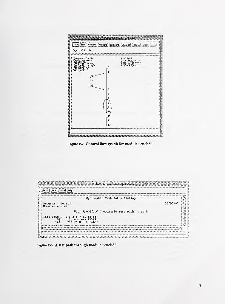
Rgure 2-2. Control flow graph for module "euclid."

Print] iSauej ;ClMe] iHelp

Program : Euclid: Module: euclid

Cyclomatic Test Paths Listing

User Specified Cyclomatic Test Path: 1 Path

04/07/97

Test Path 1 : 0 1 5 6 7 11 12 138( 1) : n>m --> FALSE

14 ( 7) : r! -0 --> FALSE

Figure 2-3. A test path through module "euclid."

that satisfies the structured testing criterion, which consists of the three tests from Figure 5-4

plus two additional tests to form a complete basis.

Input Output Correctness

X -1 Correct

ABCX 1 Correct

Rgure 5-4. Tests for "count" that satisfy statement and branch coverage.


X -1 Correct

ABCX 1 Correct

A 0 Correct

AB 1 Incorrect

AC 0 Incorrect

Figure 5-5. Tests for "count" that satisfy the structured testing criterion.






5.5 Weak structured testing

Weak structured testing is, as it appears, a weak variant of structured testing. It can be satis-

fied by exercising at least v(G) different paths through the control flow graph while simulta-

neously covering aU branches, however the requirement that the paths form a basis is dropped.

Structured testing subsumes weak structured testing, but not the reverse. Weak structured

testing is much easier to perform manually than structured testing, because there is no need to

do linear algebra on path vectors. Thus, weak structured testing was a way to get some of the

benefits of structured testing at a significantly lesser cost before automated support for struc-

tured testing was available, and is still worth considering for programming languages with no

automated structured testing support. In some older literature, no distinction is made between

the two criteria.

Of the three properties of structured testing discussed in section 5.2, two are shared by weak

structured testing. It subsumes statement and branch coverage, which provides a base level of

error detection effectiveness. It also requires testing proportional to complexity, which con-

centrates testing on the most error-prone software and supports precise test planning and mon-

itoring. However, it does not require all decision outcomes to be tested independeiitiy, and

37

6 The Baseline Method

The baseline method, described in this section, is a technique for identifying a set of control

paths to satisfy the structured testing criterion. The technique results in a basis set of test

paths through the module being tested, equal in number to the cyclomatic complexity of the

module. As discussed in section 2, the paths in a basis are independent and generate all paths

via linear combinations. Note that "the baseUne method" is different from "basis path test-

ing." Basis path testing, another name for structured testing, is the requirement that a basis set

of paths should be tested. The baseline method is one way to derive a basis set of paths. Theword "baseline" comes from the first path, which is typically selected by the tester to repre-

sent the "baseline" functionality of the module. The basehne method provides support for

structured testing, since it gives a specific technique to identify an adequate test set rather than

resorting to trial and error until the criterion is satisfied.

6. 1 Generating a basis set ofpaths

The idea is to start with a baseline path, then vary exactly one decision outcome to generate

each successive path until all decision outcomes have been varied, at which time a basis will

have been generated. To understand the mathematics behind the technique, a simplified ver-

sion of the method will be presented and prove that it generates a basis [WATS0N5]. Then,

the general technique that gives more freedom to the tester when selecting paths will be

described. Poole describes and analyzes an independently derived variant in [NIST5737].

6.2 The simplified baseline method,


Readers not interested in theory may prefer to skip to section 6.3 where a more practical pre-


In addition to a basis set of paths, which is a basis for the rows of the path/edge matrix if all

possible paths were represented, it is possible to also consider a basis set of edges, which is a

basis for the columns of the same matrix. Since row rank equals column rank, the cyclomatic

complexity is also the number of edges in every edge basis. The overall approach of this sec-

tion is to first select a basis set of edges, then use that set in the algorithm to generate each

successive path, and finally use the resulting path/edge matrix restricted to basis columns to

show that the set of generated paths is a basis.

41

NIST Special Publication 500-235

Structured Testing: A Testing Methodology

Using the Cyciomatic Complexity Metric

Dolores R. Wallace, Editor

Computer Systems Laboratory

National Institute of Standards and Technology

Gaithersburg, MD 20899-0001

Arthur H. Watson

Thomas J. McCabe

McCabe & Associates

Columbia, MD 21045

NIST Contract 43NANB517266

August 1996

U.S. Department of CommerceMichael Kantor, Secretary

Technology Administration

Mary L. Good, Under Secretary for Technology

National Institute of Standards and Technology

Arati Prabhakar. Director

Reports on Computer Systems Technology

The National Institute of Standards and Technology (NIST) has a unique responsibility for computer

systems technology within the Federal government. NIST's Computer Systems Laboratory (CSL) devel-

ops standards and guidelines, provides technical assistance, and conducts research for computers and

related telecommunications systems to achieve more effective utilization of Federal information technol-

ogy resources. CSL's responsibilities include development of technical, management, physical, and ad-

ministrative standards and guidelines for the cost-effective security and privacy of sensitive unclassified

information processed in Federal computers. CSL assists agencies in developing security plans and in

improving computer security awareness training. This Special Publication 500 series reports CSL re-

search and guidelines to Federal agencies as well as to organizations in industry, government, and

academia.

National Institute of Standards and Technology Special Publication 500-235Natl. Inst. Stand. Technol. Spec. Publ. 500-235, 119 pages (August 1996)

CODEN: NSPUE2

U.S. GOVERNMENT PRINTING OFFICEWASHINGTON: 1996

For sale by the Superintendent of Documents, U.S. Government Printing Office, Washington, DC 20402

Abstract

The purpose of this document is to describe the structured testing methodology for software

testing, also known as basis path testing. Based on the cyclomatic complexity measure of

McCabe, structured testing uses the control flow structure of software to establish path cover-

age criteria. The resultant test sets provide more thorough testing than statement and branch

coverage. Extensions of the fundamental structured testing techniques for integration testing

and object-oriented systems are also presented. Several related software complexity metrics

are described. Summaries of technical papers, case studies, and empirical results are presented

in the appendices.

Keywords

Basis path testing, cyclomatic complexity, McCabe, object oriented, software development,

software diagnostic, software metrics, software testing, structured testing

Acknowledgments

The authors acknowledge the contributions by Patricia McQuaid to Appendix A of this report.

Disclaimer

Certain trade names and company names are mentioned in the text or identified. In no case

does such identification imply recommendation or endorsement by the National Institute

of Standards and Technology, nor does it imply that the products are necessarily the best

available for the purpose.

iii

Executive Summary

This document describes the structured testing methodology for software testing and related

software complexity analysis techniques. The key requirement of structured testing is that all

decision outcomes must be exercised independently during testing. The number of tests

required for a software module is equal to the cyclomatic complexity of that module. The

original structured testing document [NBS99] discusses cyclomatic complexity and the basic

testing technique. This document gives an expanded and updated presentation of those topics,

describes several new complexity measures and testing strategies, and presents the experience

gained through the practical application of these techniques.

The software complexity measures described in this document are: cyclomatic complexity,

module design complexity, integration complexity, object integration complexity, actual com-

plexity, realizable complexity, essential complexity, and data complexity. The testing tech-

niques are described for module testing, integration testing, and object-oriented testing.

A significant amount of practical advice is given concerning the application of these tech-

niques. The use of complexity measurement to manage software reliability and maintainabil-

ity is discussed, along with strategies to control complexity during maintenance. Methods to

apply the testing techniques are also covered. Both manual techniques and the use of auto-

mated support are described.

Many detailed examples of the techniques are given, as well as summaries of technical papers

and case studies. Experimental results are given showing that structured testing is superior to

statement and branch coverage testing for detecting errors. The bibliography lists over 50 ref-

erences to related information.

V

f

I

!

i

CONTENTS

Abstract iii

Keywords iii

Acknowledgments iii

Executive Summary v

1 Introduction 1

1.1 Software testing 1

1.2 Software complexity measurement 2

1.3 Relationship between complexity and testing 3

1.4 Document overview and audience descriptions 4

2 Cyclomatic Complexity 7

2.1 Control flow graphs 7

2.2 Definition of cyclomatic complexity, v(G) 10

2.3 Characterization of v(G) using a basis set of control flow paths 11

2.4 Example of v(G) and basis paths 13

2.5 Limiting cyclomatic complexity to 10 15

3 Examples of Cyclomatic Complexity 17

3.1 Independence of complexity and size ...17

3.2 Several flow graphs and their complexity 17

4 Simplified Complexity Calculation 23

4.1 Counting predicates 23

4.2 Counting flow graph regions 28

4.3 Use of automated tools 29

5 Structured Testing 31

5.1 The structured testing criterion 31

5.2 Intuition behind structured testing 32

vii

5.3 Complexity and reliability 34

5.4 Structured testing example 34

l i' J ' 5.5 Weak structured testing 37

5.6 Advantages of automation 38

5.7 Critical software 39

6 The Baseline Method 41

6. 1 Generating a basis set of paths 41

6.2 The simplified baseline method 41

, 6.3 The baseline method in practice 42

6.4 Example of the baseline method 44

6.5 Completing testing with the baseline method 46

7 Integration Testing 47

7. 1 Integration strategies 47

7.2 Combining module testing and integration testing 48

7.3 Generalization of module testing criteria 49

7.4 Module design complexity 50

* 7.5 Integration complexity 54

7.6 Incremental integration 57

8 Testing Object-Oriented Programs 59

8. 1 Benefits and dangers of abstraction 59

8.2 Object-oriented module testing 60

'

. 8.3 Integration testing of object-oriented programs 61

8.4 Avoiding unnecessary testing 65

9 Complexity Reduction 67

9.1 Actual complexity and realizable complexity 67

9.2 Removing control dependencies 71

9.3 Trade-offs when reducing complexity 74

10 Essential Complexity 79

' 10.1 Structured programming and maintainability 79

10.2 Definition of essential complexity, ev(G). 80

10.3 Examples of essential complexity 81

11 Maintenance 83

11.1 Effects of changes on complexity 83

11.1.1 Effect of changes on cyclomatic complexity 83

11.1.2 Effect of changes on essential complexity 83

1 1.1.3 Incremental reengineering 84

1 1.2 Retesting at the path level 85

11.3 Data complexity 85

1 1.4 Reuse of testing information 86

12 Summary by Lifecycle Process 87

12.1 Design process 87

12.2 Coding process 87

12.3 Unit testing process 87

12.4 Integration testing process 87

12.5 Maintenance process 88

13 References 89

Appendix A Related Case Studies 95

A.l Myers 95

A.2 Schneidewind and Hoffman 95

A.3 Walsh 96

A.4 Henry, Kafura, and Harris 96

A.5 Sheppard and Kruesi 96

A.6 Carver 97

A.7 Kafura and Reddy 97

A. 8 Gibson and Senn 98

A.9 Ward 99

A.lOCaldiera and Basili 99

A. 11 Gill andKemerer 99

A. 12 Schneidewind 100

A. 13 Case study at Stratus Computer 101

A. 14 Case study at Digital Equipment Corporation 101

A. 15 Case study at U.S. Army Missile Command 102

A. 16 Coleman et al 102

A. 17 Case study at the AT&T Advanced Software Construction Center 103

A. 18 Case study at Sterling Software 103

A. 19 Case Study at GTE Government Systems 103

A.20 Case study at Elsag Bailey Process Automation 103

A.21 Koshgoftaar et al 1 04

ix

Appendix B Extended Example 105

B.l Testing the blackjack program 105

B.2 Experimental comparison of structured testing and branch coverage 112

1 Introduction

1.1 Software testing

This document describes the structured testing methodology for software testing. Software

testing is the process of executing software and comparing the observed behavior to the

desired behavior. The major goal of software testing is to discover errors in the software

[MYERS2], with a secondary goal of building confidence in the proper operation of the soft-

ware when testing does not discover errors. The conflict between these two goals is apparent

when considering a testing process that did not detect any errors. In the absence of other

information, this could mean either that the software is high quality or that the testing process

is low quality. There are many approaches to software testing that attempt to control the qual-

ity of the testing process to yield useful information about the quality of the software being

tested.

Although most testing research is concentrated on finding effective testing techniques, it is

also important to make software that can be effectively tested. It is suggested in [VOAS] that

software is testable if faults are likely to cause failure, since then those faults are most likely to

be detected by failure during testing. Several programming techniques are suggested to raise

testability, such as minimizing variable reuse and maximizing output parameters. In [BER-

TOLINO] it is noted that although having faults cause failure is good during testing, it is bad

after delivery. For a more intuitive testability property, it is best to maximize the probability

of faults being detected during testing while minimizing the probability of faults causing fail-

ure after delivery. Several programming techniques are suggested to raise testability, includ-

ing assertions that observe the internal state of the software during testing but do not affect the

specified output, and multiple version development [BRILLIANT] in which any disagreement

between versions can be reported during testing but a majority voting mechanism helps

reduce the likelihood of incorrect output after delivery. Since both of those techniques are fre-

quently used to help construct reliable systems in practice, this version of testability may cap-

ture a significant factor in software development.

For large systems, many errors are often found at the beginning of the testing process, with the

observed error rate decreasing as errors are fixed in the software. When the observed error

rate during testing approaches zero, statistical techniques are often used to determine a reason-

able point to stop testing [MUSA]. This approach has two significant weaknesses. First, the

testing effort cannot be predicted in advance, since it is a function of the intermediate results

of the testing effort itself. A related problem is that the testing schedule can expire long

before the error rate drops to an acceptable level. Second, and perhaps more importantly, the

statistical model only predicts the estimated error rate for the underlying test case distribution

1

being used during the testing process. It may have little or no connection to the likelihood of

errors manifesting once the system is delivered or to the total number of errors present in the

software.

Another common approach to testing is based on requirements analysis. A requirements specifi-

cation is converted into test cases, which are then executed so that testing verifies system behav-

ior for at least one test case within the scope of each requirement. Although this approach is an

important part of a comprehensive testing effort, it is certainly not a complete solution. Even

setting aside the fact that requirements documents are notoriously error-prone, requirements are

written at a much higher level of abstraction than code. This means that there is much more

detail in the code than the requirement, so a test case developed from a requirement tends to

exercise only a small fraction of the software that implements that requirement. Testing only at

the requirements level may miss many sources of error in the software itself.

The structured testing methodology falls into another category, the white box (or code-based, or

glass box) testing approach. In white box testing, the software implementation itself is used to

guide testing. A common white box testing criterion is to execute every executable statement

during testing, and verify that the output is correct for all tests. In the more rigorous branch cov-

erage approach, every decision outcome must be executed during testing. Structured testing is

still more rigorous, requiring that each decision outcome be tested independently. A fundamen-

tal strength that all white box testing strategies share is that the entire software implementation

is taken into account during testing, which facilitates error detection even when the software

specification is vague or incomplete. A corresponding weakness is that if the software does not

implement one or more requirements, white box testing may not detect the resultant errors of

omission. Therefore, both white box and requirements-based testing are important to an effec-

tive testing process. The rest of this document deals exclusively with white box testing, concen-

trating on the structured testing methodology.

1.2 Software complexity measurement

Software complexity is one branch of software metrics that is focused on direct measurement of

software attributes, as opposed to indirect software measures such as project milestone status

and reported system failures. There are hundreds of software complexity measures [ZUSE],

ranging from the simple, such as source lines of code, to the esoteric, such as the number of

variable definition/usage associations.

An important criterion for metrics selection is uniformity of application, also known as "open

reengineering." The reason "open systems" are so popular for commercial software applica-

tions is that the user is guaranteed a certain level of interoperability—the applications work

together in a common framework, and applications can be ported across hardware platforms

with minimal impact. The open reengineering concept is similar in that the abstract models

2

used to represent software systems should be as independent as possible of implementation

characteristics such as source code formatting and programming language. The objective is to

be able to set complexity standards and interpret the resultant numbers uniformly across

projects and languages. A particular complexity value should mean the same thing whether it

was calculated from source code written in Ada, C, FORTRAN, or some other language. The

most basic complexity measure, the number of lines of code, does not meet the open reengi-

neering criterion, since it is extremely sensitive to programming language, coding style, and

textual formatting of the source code. The cyclomatic complexity measure, which measures

the amount of decision logic in a source code function, does meet the open reengineering cri-

terion. It is completely independent of text formatting and is nearly independent of program-

ming language since the same fundamental decision structures are available and uniformly

used in all procedural programming languages [MCCABE5].

Ideally, complexity measures should have both descriptive and prescriptive components.

Descriptive measures identify software that is error-prone, hard to understand, hard to modify,

hard to test, and so on. Prescriptive measures identify operational steps to help control soft-

ware, for example splitting complex modules into several simpler ones, or indicating the

amount of testing that should be performed on given modules.

1.3 Relationship between complexity and testing

There is a strong connection between complexity and testing, and the structured testing meth-

odology makes this connection explicit.

First, complexity is a common source of error in software. This is true in both an abstract and

a concrete sense. In the abstract sense, complexity beyond a certain point defeats the human

mind's ability to perform accurate symbolic manipulations, and errors result. The same psy-

chological factors that limit people's ability to do mental manipulations of more than the infa-

mous "7 +/- 2" objects simultaneously [MILLER] apply to software. Structured programming

techniques can push this barrier further away, but not eliminate it entirely. In the concrete

sense, numerous studies and general industry experience have shown that the cyclomatic com-

plexity measure correlates with errors in software modules. Other factors being equal, the

more complex a module is, the more likely it is to contain errors. Also, beyond a certain

threshold of complexity, the likelihood that a module contains errors increases sharply. Given

this information, many organizations limit the cyclomatic complexity of their software mod-

ules in an attempt to increase overall reliability. A detailed recommendation for complexity

limitation is given in section 2.5.

Second, complexity can be used directly to allocate testing effort by leveraging the connection

between complexity and error to concentrate testing effort on the most error-prone software.

In the structured testing methodology, this allocation is precise—the number of test paths

3

required for each software module is exactly the cyclomatic complexity. Other commonwhite box testing criteria have the inherent anomaly that they can be satisfied with a small

number of tests for arbitrarily complex (by any reasonable sense of "complexity") software as

shown in section 5.2.

1.4 Document overview and audience descriptions

• Section 1 gives an overview of this document. It also gives some general information about

software testing, software complexity measurement, and the relationship between the two.

• Section 2 describes the cyclomatic complexity measure for software, which provides the

foundation for structured testing.

• Section 3 gives some examples of both the applications and the calculation of cyclomatic

complexity.

• Section 4 describes several practical shortcuts for calculating cyclomatic complexity.

• Section 5 defines structured testing and gives a detailed example of its application.

• Section 6 describes the Baseline Method, a systematic technique for generating a set of test

paths that satisfy structured testing.

• Section 7 describes structured testing at the integration level.

• Section 8 describes structured testing for object-oriented programs.

• Section 9 discusses techniques for identifying and removing unnecessary complexity and

the impact on testing.

• Section 10 describes the essential complexity measure for software, which quantifies the

extent to which software is poorly structured.

• Section 1 1 discusses software modification, and how to apply structured testing to pro-

grams during maintenance.

• Section 12 summarizes this document by software lifecycle phase, showing where each

technique fits into the overall development process.

• Appendix A describes several related case studies.

• Appendix B presents an extended example of structured testing. It also describes an exper-

imental design for comparing structural testing strategies, and applies that design to illus-

trate the superiority of structured testing over branch coverage.

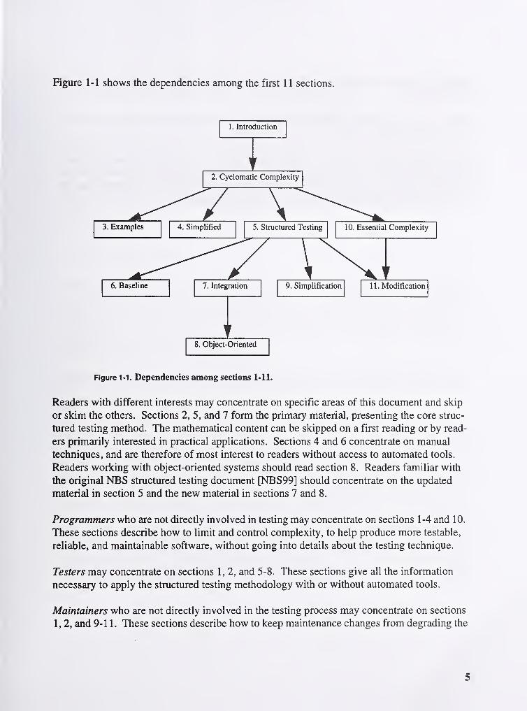
Figure 1-1 shows the dependencies among the first 1 1 sections.

8. Object-Oriented

Figure 1-1. Dependencies among sections 1-11.

Readers with different interests may concentrate on specific areas of this document and skip

or skim the others. Sections 2, 5, and 7 form the primary material, presenting the core struc-

tured testing method. The mathematical content can be skipped on a first reading or by read-

ers primarily interested in practical appUcations. Sections 4 and 6 concentrate on manual

techniques, and are therefore of most interest to readers without access to automated tools.

Readers working with object-oriented systems should read section 8. Readers familiar with

the original NBS structured testing document [NBS991 should concentrate on the updated

material in section 5 and the new material in sections 7 and 8.

Programmers who are not directly involved in testing may concentrate on sections 1-4 and 10.

These sections describe how to limit and control complexity, to help produce more testable,

reliable, and maintainable software, without going into details about the testing technique.

Testers may concentrate on sections 1, 2, and 5-8. These sections give all the information

necessary to apply the structured testing methodology with or without automated tools.

Maintainers who are not directly involved in the testing process may concentrate on sections

1, 2, and 9-11. These sections describe how to keep maintenance changes from degrading the

5

testability, reliability, and maintainability of software, without going into details about the

testing technique.

Project Leaders and Managers should read through the entire document, but may skim over

the details in sections 2 and 5-8.

Quality Assurance, Methodology, and Standards professionals may skim the material in sec-

tions 1 , 2, and 5 to get an overview of the method, then read section 12 to see where it fits into

the software lifecycle. The Appendices also provide important information about experience

with the method and implementation details for specific languages.

2 Cyclomatic Complexity

Cyclomatic complexity [MCCABEl] measures the amount of decision logic in a single soft-

ware module. It is used for two related purposes in the structured testing methodology. First,

it gives the number of recommended tests for softwaie. Second, it is used during all phases of

the software lifecycle, beginning with design, to keep software reliable, testable, and manage-

able. Cyclomatic complexity is based entirely on the structure of software's control flow

graph.

2.1 Controlflow graphs

Control flow graphs describe the logic structure of software modules. A module corresponds

to a single function or subroutine in typical languages, has a single entry and exit point, and is

able to be used as a design component via a call/return mechanism. This document uses C as

the language for examples, and in C a module is a function. Each flow graph consists of

nodes and edges. The nodes represent computational statements or expressions, and the edges

represent transfer of control between nodes.

Each possible execution path of a software module has a corresponding path from the entry to

the exit node of the module's control flow graph. This correspondence is the foundation for

the structured testing methodology.

As an example, consider the C function in Figure 2-1, which implements Euclid's algorithm

for finding greatest common divisors. The nodes are numbered AO through A 13. The control

flow graph is shown in Figure 2-2, in which each node is numbered 0 through 13 and edges

are shown by lines connecting the nodes. Node 1 thus represents the decision of the "if state-

ment with the true outcome at node 2 and the false outcome at the collection node 5. The deci-

sion of the "while" loop is represented by node 7, and the upward flow of control to the next

iteration is shown by the dashed line from node 10 to node 7. Figure 2-3 shows the path

resulting when the module is executed with parameters 4 and 2, as in "euclid(4,2)." Execution

begins at node 0, the beginning of the module, and proceeds to node 1, the decision node for

the "if statement. Since the test at node 1 is false, execution transfers directly to node 5, the

collection node of the "if statement, and proceeds to node 6. At node 6, the value of "r" is

calculated to be 0, and execution proceeds to node 7, the decision node for the "while" state-

ment. Since the test at node 7 is false, execution transfers out of the loop directly to node 11,

7

then proceeds to node 12, returning the result of 2. The actual return is modeled by execution

proceeding to node 13, the module exit node.

Prifitl fSavej [Convert] jciose] pHelp]

ProgramFileLanguageModule ModuleLetter Name

Euclideuclid.cinstc

Annotated Source Listing

01/15/96

Start Num ofv(G) ev(G) iv(G) Line Lines

A euclid 3 1 1

2 AO euclid(int m, int n)3 (/* Assuming m and n both greater than 0,4 * return their greatest common divisor.5 * Enforce m >= n for efficiency.6 */7 int r;8 Al if (n > m) {

9 A2 r - m;10 A3 m - n;11 A4 n = r;12 )

13 A5 A6 r = m % n; /* m modulo n */14 A7 while (r ! = 0) {

15 A8 m = n;16 A9 n = r;17 AlO r = m % n; /* m modulo n */18 All }

19 A12 return n;20 A13 )

19

Figure 2-1. Annotated source listing for module "euclid."

8

Plotj [Savel [convert] jiorwd] jiackuardl [Enlarge] [Reduce| fciosel [ttelp]

Page 1 of 1 2X

.12

Figure 2-2. Control flow graph for module "euclid."

i<pun EuclM

{Print| [Save[(pjnuert

|jciose] jhlelpj

Cyclomatic Test Paths Listing

Program : Euclid 01/15/96Module: euclid

User Specified Cyclomatic Test Path: 1 Path

Test Path 1:01 2 3 4 5 6 7 8 9 10 7 8 9 10 7 11 12 138( 1) n>m ==> TRUE

14( 7) r! =0 —> TRUE14( 7) r! =0 —> TRUE14( 7) r! =0 ==> FALSE

W-F^^ =Figure 2-3. A test path through module "eucUd."

2.2 Definition of cyclomatic complexity, v(G)

Cyclomatic complexity is defined for each module to be e - n + 2, where e and n are the num-

ber of edges and nodes in the control flow graph, respectively. Thus, for the Euclid's algo-

rithm example in section 2.1, the complexity is 3 (15 edges minus 14 nodes plus 2).

Cyclomatic complexity is also known as v(G), where v refers to the cyclomatic number in

graph theory and G indicates that the complexity is a function of the graph.

The word "cyclomatic" comes from the number of fundamental (or basic) cycles in con-

nected, undirected graphs [BERGE]. More importantly, it also gives the number of indepen-

dent paths through strongly connected directed graphs. A strongly connected graph is one in

which each node can be reached from any other node by following directed edges in the

graph. The cyclomatic number in graph theory is defined as e - n + 1 . Program control flow

graphs are not strongly connected, but they become strongly connected when a "virtual edge"

is added connecting the exit node to the entry node. The cyclomatic complexity definition for

program control flow graphs is derived from the cyclomatic number formula by simply add-

ing one to represent the contribution of the virtual edge. This definition makes the cyclomatic

complexity equal the number of independent paths through the standard control flow graph

model, and avoids explicit mention of the virtual edge.

Figure 2-4 shows the control flow graph of Figure 2-2 with the virtual edge added as a dashed

line. This virtual edge is not just a mathematical convenience. Intuitively, it represents the

control flow through the rest of the program in which the module is used. It is possible to cal-

culate the amount of (virtual) control flow through the virtual edge by using the conservation

of flow equations at the entry and exit nodes, showing it to be the number of times that the

module has been executed. For any individual path through the module, this amount of flow is

exactly one. Although the virtual edge will not be mentioned again in this document, note that

since its flow can be calculated as a linear combination of the flow through the real edges, its

presence or absence makes no difference in determining the number of linearly independent

paths through the module.

10

Figure 2-4. Control flow graph with virtual edge.

2.3 Characterization ofv(G) using a basis set of controlflow paths

Cyclomatic complexity can be characterized as the number of elements of a basis set of con-

trol flow paths through the module. Some familiarity with linear algebra is required to follow

the details, but the point is that cyclomatic complexity is precisely the minimum number of

paths that can, in (linear) combination, generate all possible paths through the module. To see

this, consider the following mathematical model, which gives a vector space corresponding to

each flow graph.

Each path has an associated row vector, with the elements corresponding to edges in the flow

graph. The value of each element is the number of times the edge is traversed by the path.

Consider the path described in Figure 2-3 through the graph in Figure 2-2. Since there are 15

edges in the graph, the vector has 15 elements. Seven of the edges are traversed exactly once

as part of the path, so those elements have value 1 . The other eight edges were not traversed as

part of the path, so they have value 0.

11

Considering a set of several paths gives a matrix in which the columns correspond to edges

and the rows correspond to paths. From linear algebra, it is known that each matrix has a

unique rank (number of linearly independent rows) that is less than or equal to the number of

columns. This means that no matter how many of the (potentially infinite) number of possible

paths are added to the matrix, the rank can never exceed the number of edges in the graph. In

fact, the maximum value of this rank is exactly the cyclomatic complexity of the graph. Aminimal set of vectors (paths) with maximum rank is known as a basis, and a basis can also be

described as a linearly independent set of vectors that generate all vectors in the space by lin-

ear combination. This means that the cyclomatic complexity is the number of paths in any

independent set of paths that generate all possible paths by linear combination.

Given any set of paths, it is possible to determine the rank by doing Gaussian Elimination on

the associated matrix. The rank is the number of non-zero rows once elimination is complete.

If no rows are driven to zero during elimination, the original paths are linearly independent. If

the rank equals the cyclomatic complexity, the original set of paths generate all paths by linear

combination. If both conditions hold, the original set of paths are a basis for the flow graph.

There are a few important points to note about the linear algebra of control flow paths. First,

although every path has a corresponding vector, not every vector has a corresponding path.

This is obvious, for example, for a vector that has a zero value for all elements corresponding

to edges out of the module entry node but has a nonzero value for any other element cannot

correspond to any path. Slightly less obvious, but also true, is that linear combinations of vec-

tors that correspond to actual paths may be vectors that do not correspond to actual paths.

This follows from the non-obvious fact (shown in section 6) that it is always possible to con-

struct a basis consisting of vectors that correspond to actual paths, so any vector can be gener-

ated from vectors corresponding to actual paths. This means that one can not just find a basis

set of vectors by algebraic methods and expect them to correspond to paths—one must use a

path-oriented technique such as that of section 6 to get a basis set of paths. Finally, there are a

potentially infinite number of basis sets of paths for a given module. Each basis set has the

same number of paths in it (the cyclomatic complexity), but there is no limit to the number of

different sets of basis paths. For example, it is possible to start with any path and construct a

basis that contains it, as shown in section 6.3.

The details of the theory behind cyclomatic complexity are too mathematically complicated to

be used directly during software development. However, the good news is that this mathe-

matical insight yields an effective operational testing method in which a concrete basis set of

paths is tested: structured testing.

12

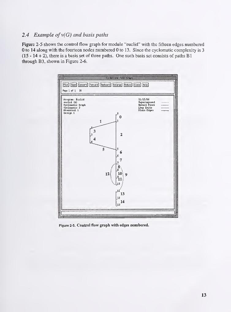
2.4 Example ofv(G) and basis paths

Figure 2-5 shows the control flow graph for module "euclid" with the fifteen edges numbered

0 to 14 along with the fourteen nodes numbered 0 to 13. Since the cyclomatic complexity is 3

(15 - 14 + 2), there is a basis set of three paths. One such basis set consists of paths B

1

through B3, shown in Figure 2-6.

Cydlomatic Row Graph

|Plot[ [Save~|IConvert] [Foruard] jiackuard) jEnlarse] |Recluce| [ciose] |Hc1p|

Pago 1 of 1 3X

Program: EuclideucLid (A)

Cyclomatic GraphCyclomatic 3

Essential 1

Design 1

12

13)

1413

01/15/9SSuperinposedUpward FlowsLoop ExitsPlain Edges

Figure 2-5. Control flow graph with edges numbered.

13

Module: euclid

Basis Test Paths: 3 Paths

Test Path Bl: 0 1 5 6 7 11 12 138{ 1) n>m ==> FALSE

14 ( 7) r!=0 ==> FALSE

Test Path B2

:

0 1 2 3 4 5 6 7 11 12 138( 1) n>m ==> TRUE

14 ( 7) r!=0 ==> FALSE

Test Path B3

:

0 1 5 6 7 8 9 10 7 11 128( 1) n>m ==> FALSE

14( 7) r!=0 ==> TRUE14{ 7) r!=0 ==> FALSE

Figure 2-6. A basis set of paths, Bl through B3.

Any arbitrary path can be expressed as a linear combination of the basis paths B 1 through B3.

For example, the path P shown in Figure 2-7 is equal to B2 - 2 * B 1 + 2 * B3.

Module: euclid

User Specified Path: 1 Path

Test Path P: 0 1 2 3 4 5 6 7 8 9 10 7 8 9 10 7 11 12 13

8( 1) : n>m = => TRUE14 ( 7) : r!=0 ==> TRUE14 ( 7) : r!=0 ==> TRUE14 ( 7) : r!=0 ==> FALSE

Figure 2-7. Path P.

To see this, examine Figure 2-8, which shows the number of times each edge is executed

along each path.

Path/Edge 0 1 2 3 4 5 6 7 8 9 10 11 12

Bl 1 0 1 0 0 0 1 1 0 1 0 0 0

B2 1 1 0 1 1 1 1 1 0 1 0 0 0

B3 1 0 1 0 0 0 1 1 1 1 1 1 1

P 1 1 0 1 1 1 1 1 2 1 2 2 2

Figure 2-8. Matrix of edge incidence for basis paths B1-B3 and other path P.

One interesting property of basis sets is that every edge of a flow graph is traversed by at least

one path in every basis set. Put another way, executing a basis set of paths will always cover

every control branch in the module. This means that to cover all edges never requires more

14

than the cyclomatic complexity number of paths. However, executing a basis set just to cover

all edges is overkill. Covering all edges can usually be accomplished with fewer paths. In

this example, paths B2 and B3 cover all edges without path B 1 . The relationship betweenbasis paths and edge coverage is discussed further in section 5.

Note that apart from forming a basis together, there is nothing special about paths B 1 through

B3. Path P in combination with any two of the paths B 1 through B3 would also form a basis.

The fact that there are many sets of basis paths through most programs is important for testing,

since it means it is possible to have considerable freedom in selecting a basis set of paths to

test.

2.5 Limiting cyclomatic complexity to 10

There are many good reasons to limit cyclomatic complexity. Overly complex modules are

more prone to error, are harder to understand, are harder to test, and are harder to modify.

Deliberately limiting complexity at all stages of software development, for example as a

departmental standard, helps avoid the pitfalls associated with high complexity software.

Many organizations have successfully implemented complexity limits as part of their software

programs. The precise number to use as a limit, however, remains somewhat controversial.

The original limit of 10 as proposed by McCabe has significant supporting evidence, but lim-

its as high as 15 have been used successfully as well. Limits over 10 should be reserved for

projects that have several operational advantages over typical projects, for example experi-

enced staff, formal design, a modem programming language, structured programming, code

walkthroughs, and a comprehensive test plan. In other words, an organization can pick a com-

plexity limit greater than 10, but only if it is sure it knows what it is doing and is willing to

devote the additional testing effort required by more complex modules.

Somewhat more interesting than the exact complexity limit are the exceptions to that limit.

For example, McCabe originally recommended exempting modules consisting of single mul-

tiway decision ("switch" or "case") statements from the complexity limit. The multiway deci-

sion issue has been interpreted in many ways over the years, sometimes with disastrous

results. Some naive developers wondered whether, since multiway decisions qualify for

exemption from the complexity limit, the complexity measure should just be altered to ignore

them. The result would be that modules containing several multiway decisions would not be

identified as overly complex. One developer started reporting a "modified" complexity in

which cyclomatic complexity was divided by the number of multiway decision branches. The

stated intent of this metric was that multiway decisions would be treated uniformly by having

them contribute the average value of each case branch. The actual result was that the devel-

oper could take a module with complexity 90 and reduce it to "modified" complexity 10 sim-

ply by adding a ten-branch multiway decision statement to it that did nothing.

15

Consideration of the intent behind complexity limitation can keep standards policy on track.

There are two main facets of complexity to consider: the number of tests and everything else

(reliability, maintainability, understandability, etc.). Cyclomatic complexity gives the numberof tests, which for a multiway decision statement is the number of decision branches. Anyattempt to modify the complexity measure to have a smaller value for multiway decisions will

result in a number of tests that cannot even exercise each branch, and will hence be inadequate

for testing purposes. However, the pure number of tests, while important to measure and con-

trol, is not a major factor to consider when limiting complexity. Note that testing effort is

much more than just the number of tests, since that is multiplied by the effort to construct each

individual test, bringing in the other facet of complexity. It is this correlation of complexity

with reliability, maintainability, and understandability that primarily drives the process to

limit complexity.

Complexity limitation affects the allocation of code among individual software modules, lim-

iting the amount of code in any one module, and thus tending to create more modules for the

same application. Other than complexity limitation, the usual factors to consider when allo-

cating code among modules are the cohesion and coupling principles of structured design: the

ideal module performs a single conceptual function, and does so in a self-contained manner

without interacting with other modules except to use them as subroutines. Complexity limita-

tion attempts to quantify an "except where doing so would render a module too complex to

understand, test, or maintain" clause to the structured design principles. This rationale pro-

vides an effective framework for considering exceptions to a given complexity limit.

Rewriting a single multiway decision to cross a module boundary is a clear violation of struc-

tured design. Additionally, although a module consisting of a single multiway decision mayrequire many tests, each test should be easy to construct and execute. Each decision branch

can be understood and maintained in isolation, so the module is likely to be reliable and main-

tainable. Therefore, it is reasonable to exempt modules consisting of a single multiway deci-

sion statement from a complexity limit. Note that if the branches of the decision statement

contain complexity themselves, the rationale and thus the exemption does not automatically

apply. However, if all branches have very low complexity code in them, it may well apply.

Although constructing "modified" complexity measures is not recommended, considering the

maximum complexity of each multiway decision branch is likely to be much more useful than

the average. At this point it should be clear that the multiway decision statement exemption is

not a bizarre anomaly in the complexity measure but rather the consequence of a reasoning

process that seeks a balance between the complexity limit, the principles of structured design,

and the fundamental properties of software that the complexity limit is intended to control.

This process should serve as a model for assessing proposed violations of the standard com-

plexity limit. For developers with a solid understanding of both the mechanics and the intent

of complexity limitation, the most effective policy is: "For each module, either limit cyclo-

matic complexity to 10 (as discussed earlier, an organization can substitute a similar number),

or provide a written explanation of why the limit was exceeded."

16

3 Examples of Cyclomatic Complexity

3.1 Independence ofcomplexity and size

There is a big difference between complexity and size. Consider the difference between the

cyclomatic complexity measure and the number of lines of code, a common size measure.

Just as 10 is a common limit for cyclomatic complexity, 60 is a common limit for the number

of lines of code, the somewhat archaic rationale being that each software module should fit on

one printed page to be manageable. Although the number of lines of code is often used as a

crude complexity measure, there is no consistent relationship between the two. Many mod-

ules with no branching of control flow (and hence the minimum cyclomatic complexity of

one) consist of far greater than 60 lines of code, and many modules with complexity greater

than ten have far fewer than 60 lines of code. For example, Figure 3-1 has complexity 1 and

282 lines of code, while Figure 3-9 has complexity 28 and 30 lines of code. Thus, although

the number of lines of code is an important size measure, it is independent of complexity and

should not be used for the same purposes.

3.2 Severalflow graphs and their complexity

Several actual control flow graphs and their complexity measures are presented in Figures 3-1

through 3-9, to solidify understanding of the measure. The graphs are presented in order of

increasing complexity, in order to emphasize the relationship between the complexity num-

bers and an intuitive notion of the complexity of the graphs.

17

f^"}}t^o'^tj 'porwaTjj iBaduwrdj iEfilary] ;RedCT| \c\<no\ [Mp]

\

]39 of 134 a r.

EBt^imtriJierai^m (m) i«9«cia!«i«d

Cittntl&l 1 B rlftln Eiftf ^

1

i 1

Figure 3-1 . Control flow graph with complexity 1.

Figure 3-2. Control flow graph with complexity 3.



19


Figure 3-6. Control flow graph with complexify 8.

Cycftiinattc Flow Graph

I ^l^il \l^o^^s'^t

j

Forujard}

Backuardj Enlarge] Reduce | Closej

Help

I

Page 61 of 194 3X


One essential ingredient in any testing methodology is to limit the program logic during

development so that the program can be understood, and the amount of testing required to ver-

ify the logic is not overwhelming. A developer who, ignorant of the implications of complex-

ity, expects to verify a module such as that of Figure 3-9 with a handful of tests is heading for

disaster. The size of the module in Figure 3-9 is only 30 lines of source code. The size of sev-

eral of the previous graphs exceeded 60 lines, for example the 282-line module in Figure 3-1.

In practice, large programs often have low complexity and small programs often have high

complexity. Therefore, the common practice of attempting to limit complexity by controlling

only how many lines a module will occupy is entirely inadequate. Limiting complexity

directly is a better alternative.

22

4 Simplified Complexity Calculation

Applying the e - n + 2 formula by hand is tedious and error-prone. Fortunately, there are sev-

eral easier ways to calculate complexity in practice, ranging from counting decision predicates

to using an automated tool.

4. 1 Counting predicates

If all decisions are binary and there are p binary decision predicates, v(G) = p + 1 . A binary

decision predicate appears on the control flow graph as a node with exactly two edges flowing

out of it. Starting with one and adding the number of such nodes yields the complexity. This

formula is a simple consequence of the complexity definition. A straight-line control flow

graph, which has exactly one edge flowing out of each node except the module exit node, has

complexity one. Each node with two edges out of it adds one to complexity, since the "e" in

the e - n + 2 formula is increased by one while the "n" is unchanged. In Figure 4-1, there are

three binary decision nodes (1,2, and 6), so complexity is 4 by direct application of the p + 1

formula. The original e - n + 2 gives the same answer, albeit with a bit more counting,

12 edges - 10 nodes + 2 = 4. Figure 4-2 has two binary decision predicate nodes (1 and 3), so

complexity is 3. Since the decisions in Figure 4-2 come from loops, they are represented dif-

ferently on the control flow graph, but the same counting technique applies.

Figure 4-1 . Module with complexity four.

23

Figure 4-2. Module with complexity three.

Multiway decisions can be handled by the same reasoning as binary decisions, although there

is not such a neat formula. As in the p + 1 formula for binary predicates, start with a complex-

ity value of one and add something to it for each decision node in the control flow graph. The

number added is one less than the number of edges out of the decision node. Note that for

binary decisions, this number is one, which is consistent with the p + 1 formula. For a three-

way decision, add two, and so on. In Figure 4-3, there is a four-way decision, which adds

three to complexity, as well as three binary decisions, each of which adds one. Since the mod-

ule started with one unit of complexity, the calculated complexity becomes 1 -i- 3 + 3, for a

total of 7.

Figure 4-3. Module with complexity 7.

24

In addition to counting predicates from the flow graph, it is possible to count them directly

from the source code. This often provides the easiest way to measure and control complexity

during development, since complexity can be measured even before the module is complete.

For most programming language constructs, the construct has a direct mapping to the control

flow graph, and hence contributes a fixed amount to complexity. However, constructs that

appear similar in different languages may not have identical control flow semantics, so cau-

tion is advised. For most constructs, the impact is easy to assess. An "if statement, "while"

statement, and so on are binary decisions, and therefore add one to complexity. Boolean oper-

ators add either one or nothing to complexity, depending on whether they have short-circuit

evaluation semantics that can lead to conditional execution of side-effects. For example, the

C "&&" operator adds one to complexity, as does the Ada "and then" operator, because both

are defined to use short-circuit evaluation. The Ada "and" operator, on the other hand, does

not add to complexity, because it is defined to use the full-evaluation strategy, and therefore

does not generate a decision node in the control flow graph.

Figure 4-4 shows a C code module with complexity 6. Starting with 1, each of the two "if

statements add 1 , the "while" statement adds 1 , and each of the two "&&" operators adds 1

,

for a total of 6. For reference. Figure 4-5 shows the control flow graph corresponding to Fig-

ure 4-4.

Aiwiotated iSouttM UsUng for Program SamplBs

tPrintI fSave] [Eonvert] [Hosel iHelp]

Program : SamplesFile : samples4.cLanguage: c_nppModule ModuleLetter Name


v(G) ev(G) iv(G)

1

01/16/961

Start Num of|Line Lines 1

D complexity

6

6 6 3 40 12

40 DO coraplexity6(int i, int j)41 {/* Sample module with complexity 6 */

42 Dl 02 if (i > 0 ss j > 0) {

43 03 vjhile (i > j) (

44 D4 D5 if (i % 2 SS j % 2)

45 06 printf ("%d\n", i);

46 else47 07 08 printf ("%d\n", j);48 09 i~;49 01

0

)

50 )

51 Oil D12 )

- — . . ,^

I

Figure 4-4. Code for module with complexity 6.

25

Figure 4-5. Graph for module with complexity 6.

It is possible, under special circumstances, to generate control flow graphs that do not model

the execution semantics of boolean operators in a language. This is known as "suppressing"

short-circuit operators or "expanding" full-evaluating operators. When this is done, it is

important to understand the implications on the meaning of the metric. For example, flow

graphs based on suppressed boolean operators in C can give a good high-level view of control

flow for reverse engineering purposes by hiding the details of the encapsulated and often

unstructured expression-level control flow. However, this representation should not be used

for testing (unless perhaps it is first verified that the short-circuit boolean expressions do not

contain any side effects). In any case, the important thing when calculating complexity from

source code is to be consistent with the interpretation of language constructs in the flow graph.

Multiway decision constructs present a couple of issues when calculating complexity from

source code. As with boolean operators, consideration of the control flow graph representa-

tion of the relevant language constructs is the key to successful complexity measurement of

source code. An implicit default or fall-through branch, if specified by the language, must be

taken into account when calculating complexity. For example, in C there is an implicit default

if no default outcome is specified. In that case, the complexity contribution of the "switch"

statement is exactly the number of case-labeled statements, which is one less than the total

number of edges out of the multiway decision node in the control flow graph. A less fre-

quently occurring issue that has greater impact on complexity is the distinction between

"case-labeled statements" and "case labels." When several case labels apply to the same pro-

gram statement, this is modeled as a single decision outcome edge in the control flow graph,

adding one to complexity. It is certainly possible to make a consistent flow graph model in

which each individual case label contributes a different decision outcome edge and hence also

adds one to complexity, but that is not the typical usage.

Figure 4-6 shows a C code module with complexity 5. Starting with one unit of complexity,

the switch statement has three case-labeled statements (although having five total case labels),

which, considering the implicit default fall-through, is a four-way decision that contributes

three units of complexity. The "if statement contributes one unit, for a total complexity of

five. For reference. Figure 4-7 shows the control flow graph corresponding to Figure 4-6.

Wnotatea 3<ium> UsMmi for Program Samplw

I

PrintI[Save| [conwt] jciose| jlteip|


ProgramFileLanguageModule ModuleLetter Name

Samplessampl6s4 . cc_npp

01/16/96

E complexityS

53 EO5455 El56 E257 E35859 E46061 E56263 E66465 E7 E866 E9


53 14

complexityS ( int n)(/* Sample module with complexity 5 */

if (n > 0) (

suitch(n) (

case 0: case 1: printfC'zero or one\n");brealc;

case 2: printf ("two\n")

;

break;case 3: case 4: printf ("three or four\n"

break;)

) elseprintf ( "negat ive\n" )

;

Figure 4-6. Code for module with complexity 5.

Figure 4-7. Graph for module with complexity 5.

27

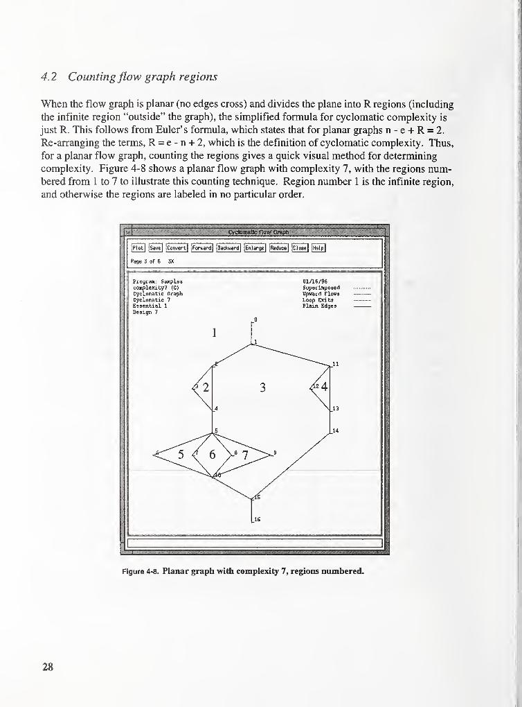
4.2 Countingflow graph regions

When the flow graph is planar (no edges cross) and divides the plane into R regions (including

the infinite region "outside" the graph), the simplified formula for cyclomatic complexity is

just R. This follows from Euler's formula, which states that for planar graphs n - e + R = 2.

Re-arranging the terms, R = e - n + 2, which is the definition of cyclomatic complexity. Thus,

for a planar flow graph, counting the regions gives a quick visual method for determining

complexity. Figure 4-8 shows a planar flow graph with complexity 7, with the regions num-bered from 1 to 7 to illustrate this counting technique. Region number 1 is the infinite region,

and otherwise the regions are labeled in no particular order.

cyclomatic flow Graph

iPlotI jSaveI|Corivert| ,Foruard| ;Backuard| ! Enlarge] -Reduce

|iClose] iHelp[

Page 3 of 6 3X

Program: Samplescomplexity7 (C)

Cyclomatic GraphCyclomatic 7

Essential 1

Design 7

01/16/96SuperimposedUpward FlowsLoop ExitsPlain Edges

Figure 4-8. Planar graph with complexity 7, regions numbered.

28

4.3 Use ofautomated tools

The most efficient and reliable way to determine complexity is through use of an automated

tool. Even calculating by hand the complexity of a single module such as that of Figure 4-9 is

a daunting prospect, and such modules often come in large groups. With an automated tool,

complexity can be determined for hundreds of modules spanning thousands of lines of code in

a matter of minutes. When dealing with existing code, automated complexity calculation and

control flow graph generation is an enabling technology. However, automation is not a pana-

cea.

::,, : :

'

., iCyclomatic Row Graph

Figure 4-9. Module with complexity 77.

The feedback from an automated tool may come too late for effective development of new

software. Once the code for a software module (or file, or subsystem) is finished and pro-

cessed by automated tools, reworking it to reduce complexity is more costly and error-prone

29

than developing the module with complexity in mind from the outset. Awareness of manual

techniques for complexity analysis helps design and build good software, rather than deferring

complexity-related issues to a later phase of the life cycle. Automated tools are an effective

way to confirm and control complexity, but they work best where at least rough estimates of

complexity are used during development. In some cases, such as Ada development, designs

can be represented and analyzed in the target programming language.

30

5 Structured Testing

Structured testing uses cyclomatic complexity and the mathematical analysis of control flow

graphs to guide the testing process. Structured testing is more theoretically rigorous and moreeffective at detecting errors in practice than other common test coverage criteria such as state-

ment and branch coverage [WATS0N5]. Structured testing is therefore suitable when reli-

ability is an important consideration for software. It is not intended as a substitute for

requirements-based "black box" testing techniques, but as a supplement to them. Structured

testing forms the "white box," or code-based, part of a comprehensive testing program, which

when quality is critical will also include requirements-based testing, testing in a simulated

production environment, and possibly other techniques such as statistical random testing.

Other "white box" techniques may also be used, depending on specific requirements for the

software being tested. Structured testing as presented in this section applies to individual soft-

ware modules, where the most rigorous code-based "unit testing" is typically performed. The

integration level Structured testing technique is described in section 7.

5. 1 The structured testing criterion

After the mathematical preliminaries of section 2 (especially Sec. 2.3), the structured testing

criterion is simply stated: Test a basis set of paths through the control flow graph of each mod-

ule. This means that any additional path through the module's control flow graph can be

expressed as a linear combination of paths that have been tested.

Note that the structured testing criterion measures the quality of testing, providing a way to

determine whether testing is complete. It is not a procedure to identify test cases or generate

test data inputs. Section 6 gives a technique for generating test cases that satisfy the structured

testing criterion.

Sometimes, it is not possible to test a complete basis set of paths through the control flow

graph of a module. This happens when some paths through the module can not be exercised

by any input data. For example, if the module makes the same exact decision twice in

sequence, no input data will cause it to vary the first decision outcome while leaving the sec-

ond constant or vice versa. This situation is explored in section 9 (especially 9.1), including

the possibilities of modifying the software to remove control dependencies or just relaxing the

testing criterion to require the maximum attainable matrix rank (known as the actual complex-

ity) whenever this differs from the cyclomatic complexity. All paths are assumed to be exer-

cisable for the initial presentation of the method.

31

A program with cyclomatic complexity 5 has the property that no set of 4 paths will suffice for

testing, even if, for example, there are 39 distinct tests that concentrate on the 4 paths. As dis-

cussed in section 2, the cyclomatic complexity gives the number of paths in any basis set. This

means that if only 4 paths have been tested for the complexity 5 module, there must be, indepen-

dent of the programming language or the computational statements of the program, at least one

additional test path that can be executed. Also, once a fifth independent path is tested, any fur-

ther paths are in a fundamental sense redundant, in that a combination of 5 basis paths will gen-

erate those further paths.

Notice that most programs with a loop have a potentially infinite number of paths, which are not

subject to exhaustive testing even in theory. The structured testing criterion establishes a com-

plexity number, v(G), of test paths that have two critical properties:

1. A test set of v(G) paths can be realized. (Again, see section 9.1 for discussion of the

more general case in which actual complexity is substituted for v(G).)

2. Testing beyond v(G) independent paths is redundantly exercising linear combinations

of basis paths.

Several studies have shown that the distribution of run time over the statements in the program

has a peculiar shape. Typically, 50% of the run time within a program is concentrated within

only 4% of the code [KNUTH]. When the test data is derived from only a requirements point of

view and is not sensitive to the internal structure of the program, it likewise will spend most of

the run time testing a few statements over and over again. The testing criterion in this document

establishes a level of testing that is inherently related to the internal complexity of a program's

logic. One of the effects of this is to distribute the test data over a larger number of independent

paths, which can provide more effective testing with fewer tests. For very simple programs

(complexity less than 5), other testing techniques seem likely to exercise a basis set of paths.

However, for more realistic complexity levels, other techniques are not likely to exercise a basis

set of paths. Exphcitly satisfying the structured testing criterion will then yield a more rigorous

set of test data.

5.2 Intuition behind structured testing

The solid mathematical foundation of structured testing has many advantages [WATSON2].First of all, since any basis set of paths covers all edges and nodes of the control flow graph, sat-

isfying the structured testing criterion automatically satisfies the weaker branch and statement

testing criteria. Technically, structured testing subsumes branch and statement coverage testing.

This means that any benefit in software reliability gained by statement and branch coverage test-

ing is automatically shared by structured testing.

32

Next, with structured testing, testing is proportional to complexity. Specifically, the minimumnumber of tests required to satisfy the structured testing criterion is exactly the cyclomatic

complexity. Given the correlation between complexity and errors, it makes sense to concen-

trate testing effort on the most complex and therefore error-prone software. Structured testing

makes this notion mathematically precise. Statement and branch coverage testing do not even

come close to sharing this property. All statements and branches of an arbitrarily complex

module can be covered with just one test, even though another module with the same com-

plexity may require thousands of tests using the same criterion. For example, a loop enclosing

arbitrarily complex code can just be iterated as many times as necessary for coverage, whereas

complex code with no loops may require separate tests for each decision outcome. With

structured testing, any path, no matter how much of the module it covers, can contribute at

most one element to the required basis set. Additionally, since the minimum required number

of tests is known in advance, structured testing supports objective planning and monitoring of

the testing process to a greater extent than other testing strategies.

Another strength of structured testing is that, for the precise mathematical interpretation of

"independent" as "linearly independent," structured testing guarantees that all decision out-

comes are tested independently. This means that unlike other common testing strategies,

structured testing does not allow interactions between decision outcomes during testing to

hide errors. As a very simple example, consider the C function of Figure 5-1. Assume that

this function is intended to leave the value of variable "a" unchanged under all circumstances,

and is thus clearly incorrect. The branch testing criterion can be satisfied with two tests that

fail to detect the error: first let both decision outcomes be FALSE, in which case the value of

"a" is not affected, and then let both decision outcomes be TRUE, in which case the value of

"a" is first incremented and then decremented, ending up with its original value. The state-

ment testing criterion can be satisfied with just the second of those two tests. Structured test-

ing, on the other hand, is guaranteed to detect this error. Since cyclomatic complexity is three,

three independent test paths are required, so at least one will set one decision outcome to

TRUE and the other to FALSE, leaving "a" either incremented or decremented and therefore

detecting the error during testing.

void funcO

{

if (condition 1)

a = a + 1;

if (condition2)

a = a- 1;

}

Figure 5-1. Example C function.

33

5.3 Complexity and reliability

Several of the studies discussed in Appendix A show a correlation between complexity and

errors, as well as a connection between complexity and difficulty to understand software.

Reliability is a combination of testing and understanding [MCCABE4]. In theory, either per-

fect testing (verify program behavior for every possible sequence of input) or perfect under-

standing (build a completely accurate mental model of the program so that any errors would

be obvious) are sufficient by themselves to ensure reliability. Given that a piece of software

has no known errors, its perceived reliability depends both on how well it has been tested and

how well it is understood. In effect, the subjective reliability of software is expressed in state-

ments such as "I understand this program well enough to know that the tests I have executed

are adequate to provide my desired level of confidence in the software." Since complexity

makes software both harder to test and harder to understand, complexity is intimately tied to

reliability. From one perspective, complexity measures the effort necessary to attain a given

level of reliability. Given a fixed level of effort, a typical case in the real world of budgets and

schedules, complexity measures reliability itself.

5.4 Structured testing example

As an example of structured testing, consider the C module "count" in Figure 5-2. Given a

string, it is intended to return the total number of occurrences of the letter 'C if the string

begins with the letter 'A.' Otherwise, it is supposed to return -1.

34

^notated Source listing for Prograni Cotmt

Print] [Save] [Convert

|

[ciose]

jHeip]

Program : CountFile : stex.cLanguage : c_nppModule ModuleLetter Name

A count

qJ/I4

5

67

8

9

1011 Al12 A213 A314 A41516 AS1718 A6 A719 A8202122 A92324 MO25 All26 A1227 A132829 A1430 A15 A163132 A17


01/18/96


30

int count (string)char * string,

•

( /* This module is incorrect. Its specification is:* If string begins with 'A' (eg "ABXCCZBZ") then* return the number of occurrences of 'C (eg 2),* otherwise return -1

.

*/int index = 0, i = 0, j =

if (string[ index] == 'A')index = index + 1

;

if (string[ index]

j = j + 1;X = 0;goto LI

;

LI

0,

{

k = 0;

'B') f

)

) elsei = -1;

return i;

if ( string [ index

1

i = i + j;k = k + 1;

j = 0;goto LI;

)

i = i + j;if (string[ index]

j = 0;goto LI

;

== 'C') {

'\0'){

Figure 5-2. Code for module "count"

The error in the "count" module is that the count is incorrect for strings that begin with the let-

ter 'A' and in which the number of occurrences of 'B' is not equal to the number of occur-

rences of 'C This is because the module is really counting 'B's rather than 'C's. It could be

fixed by exchanging the bodies of the "if statements that recognize 'B' and 'C Figure 5-3

shows the control flow graph for module "count."

35

, ; :„/.; : :, :

'

: ;,.„),:„„:

Cyclomatic Flow Graph

'1 [plot] [Save] [Conuert] [Foruard] |Backiijard| [Enlarge] iReduce] [cTose] [Help] '

t Page 1 of 1 3X

Prograjn: Count

1count (A)

1 Cyclomatic Graiph

Cyclomatic 5Essential S

: Design 1

01/18/96SuperimposedUpward Flows i s

Loop Exits -- -

Plain Edges

0 , :

/f2 / 1

.13 \|l6 1

_17

•-T'

'

Figure 5-3. Control flow graph for module "count."

The "count" module illustrates the effectiveness of structured testing. The commonly used

statement and branch coverage testing criteria can both be satisfied with the two tests in Fig-

ure 5-4, none of which detect the error. Since the complexity of "count" is five, it is immedi-

ately apparent that the tests of Figure 5-4 do not satisfy the structured testing criterion—three

additional tests are needed to test each decision independently. Figure 5-5 shows a set of tests

36

that satisfies the structured testing criterion, which consists of the three tests from Figure 5-4

plus two additional tests to form a complete basis.


X -1 Correct

ABCX 1 Correct

Figure 5-4. Tests for "count" that satisfy statement and branch coverage.


X -1 Correct

ABCX 1 Correct

A 0 Correct

AB 1 Incorrect

AC 0 Incorrect

Figure 5-5. Tests for "count" that satisfy the structured testing criterion.






5.5 Weak structured testing

Weak structured testing is, as it appears, a weak variant of structured testing. It can be satis-

fied by exercising at least v(G) different paths through the control flow graph while simulta-

neously covering all branches, however the requirement that the paths form a basis is dropped.

Structured testing subsumes weak structured testing, but not the reverse. Weak structured

testing is much easier to perform manually than structured testing, because there is no need to

do linear algebra on path vectors. Thus, weak structured testing was a way to get some of the

benefits of structured testing at a significantly lesser cost before automated support for struc-

tured testing was available, and is still worth considering for programming languages with no

automated structured testing support. In some older literature, no distinction is made between

the two criteria.

Of the three properties of structured testing discussed in section 5.2, two are shared by weak

structured testing. It subsumes statement and branch coverage, which provides a base level of

error detection effectiveness. It also requires testing proportional to complexity, which con-

centrates testing on the most error-prone software and supports precise test planning and mon-

itoring. However, it does not require all decision outcomes to be tested independently, and

37

thus may not detect errors based on interactions between decisions. Therefore, it should only

be used when structured testing itself is impractical.

5.6 Advantages ofautomation

Although structured testing can be applied manually (see section 6 for a way to generate a

basis set of paths without doing linear algebra), use of an automated tool provides several

compelling advantages. The relevant features of an automated tool are the ability to instru-

ment software to track the paths being executed during testing, the ability to report the number

of independent paths that have been tested, and the ability to calculate a minimal set of test

paths that would complete testing after any given set of tests have been run. For complex soft-

ware, the ability to report dependencies between decision outcomes directly is also helpful, as

discussed in section 9.

A typical manual process is to examine each software module being tested, derive the control

flow graph, select a basis set of tests to execute (with the technique of section 6), determine

input data that will exercise each path, and execute the tests. Although this process can cer-

tainly be used effectively, it has several drawbacks when compared with an automated pro-

cess.

A typical automated process is to leverage the "black box" functional testing in the structured

testing effort. First run the functional tests, and use the tool to identify areas of poor coverage.

Often, this process can be iterated, as the poor coverage can be associated with areas of func-

tionality, and more functional tests developed for those areas. An important practical note is

that it is easier to test statements and branches than paths, and testing a new statement or

branch is always guaranteed to improve structured testing coverage. Thus, concentrate first

on the untested branch outputs of the tool, and then move on to untested paths. Near the end

of the process, use the tool's "untested paths" or "control dependencies" outputs to derive

inputs that complete the structured testing process.

By building on a black-box, functional test suite, the automated process bypasses the labor-

intensive process of deriving input data for specific paths except for the relatively small num-

ber of paths necessary to augment the functional test suite to complete structured testing. This

advantage is even larger than it may appear at first, since functional testing is done on a com-

plete executable program, whereas deriving data to execute specific paths (or even statements)

is often only practical for individual modules or small subprograms, which leads to the

expense of developing stub and driver code. Finally, and perhaps most significantly, an auto-

mated tool provides accurate verification that the criterion was successfully met. Manual der-

ivation of test data is an error-prone process, in which the intended paths are often not

exercised by a given data set. Hence, if an automated tool is available, using it to verify and

complete coverage is very important.

38

5. 7 Critical software

Different types of software require different levels of testing rigor. All code worth developing

is worth having basic functional and structural testing, for example exercising all of the major

requirements and all of the code. In general, most commercial and government software

should be tested more stringently. Each requirement in a detailed functional specification

should be tested, the software should be tested in a simulated production environment (and is

typically beta tested in a real one), at least all statements and branches should be tested for

each module, and structured testing should be used for key or high-risk modules. Where qual-

ity is a major objective, structured testing should be applied to all modules. These testing

methods form a continuum of functional and structural coverage, from the basic to the inten-

sive. For truly critical software, however, a qualitatively different approach is needed.

Critical software, in which (for example) failure can result in the loss of human life, requires a

unique approach to both development and testing. For this kind of software, typically found

in medical and military applications, the consequences of failure are appalling [LEVESON].Even in the telecommunications industry, where failure often means significant economic

loss, cost-benefit analysis tends to limit testing to the most rigorous of the functional and

structural approaches described above.

Although the specialized techniques for critical software span the entire software lifecycle,

this section is focused on adapting structured testing to this area. Although automated tools

may be used to verify basis path coverage during testing, the techniques of leveraging func-

tional testing to structured testing are not appropriate. The key modification is to not merely

exercise a basis set of paths, but to attempt as much as possible to establish correctness of the

software along each path of that basis set. First of all, a basis set of paths facilitates structural

code walkthroughs and reviews. It is much easier to find errors in straight-line computation

than in a web of complex logic, and each of the basis paths represents a potential single

sequence of computational logic, which taken together represent the full structure of the orig-

inal logic. The next step is to develop and execute several input data sets for each of the paths

in the basis. As with the walkthroughs, these tests attempt to establish correctness of the soft-

ware along each basis path. It is important to give special attention to testing the boundary

values of all data, particularly decision predicates, along that path, as well as testing the con-

tribution of that path to implementing each functional requirement.

Although no software testing method can ensure correctness, these modifications of the struc-

tured testing methodology for critical software provide significantly more power to detect

errors in return for the significant extra effort required to apply them. It is important to note

that, especially for critical software, structured testing does not preclude the use of other tech-

niques. A notable example is exhaustive path testing: for simple modules without loops, it

may be appropriate to test all paths rather than just a basis. Many critical systems may benefit

from using several different techniques simultaneously [NIST234].

39

6 The Baseline Method

The baseline method, described in this section, is a technique for identifying a set of control

paths to satisfy the structured testing criterion. The technique results in a basis set of test

paths through the module being tested, equal in number to the cyclomatic complexity of the

module. As discussed in section 2, the paths in a basis are independent and generate all paths

via linear combinations. Note that "the baseline method" is different from "basis path test-

ing." Basis path testing, another name for structured testing, is the requirement that a basis set

of paths should be tested. The baseline method is one way to derive a basis set of paths. The

word "baseline" comes from the first path, which is typically selected by the tester to repre-

sent the "baseline" functionality of the module. The baseline method provides support for

structured testing, since it gives a specific technique to identify an adequate test set rather than

resorting to trial and error until the criterion is satisfied.

6.1 Generating a basis set ofpaths

The idea is to start with a baseline path, then vary exactly one decision outcome to generate

each successive path until all decision outcomes have been varied, at which time a basis will

have been generated. To understand the mathematics behind the technique, a simplified ver-

sion of the method will be presented and prove that it generates a basis [WATSONS] . Then,

the general technique that gives more freedom to the tester when selecting paths will be

described. Poole describes and analyzes an independently derived variant in [NIST5737].

6.2 The simplified baseline method


Readers not interested in theory may prefer to skip to section 6.2.2 where a more practical pre-


In addition to a basis set of paths, which is a basis for the rows of the path/edge matrix if all

possible paths were represented, it is possible to also consider a basis set of edges, which is a

basis for the columns of the same matrix. Since row rank equals column rank, the cyclomatic

complexity is also the number of edges in every edge basis. The overall approach of this sec-

tion is to first select a basis set of edges, then use that set in the algorithm to generate each

successive path, and finally use the resulting path/edge matrix restricted to basis columns to

show that the set of generated paths is a basis.

41

First, for every decision in the module, select an outcome with the shortest (in terms of numberof other decisions encountered) path to the module exit. Ties can be broken arbitrarily. Markthese selected decision outcomes non-basic. Call these outcomes non-basic because all other

decision outcome edges, along with the module entry edge, form the column basis. The key to

the simplified baseline method is to execute exactly one new basis edge with each successive

path. This is possible because from any node in the control flow graph, there is a path to the exit

node that avoids all basis columns (taking the non-basic outcome of every decision encoun-

tered, which also gives a shortest path in terms of decisions encountered to the exit).

The simplified baseline algorithm can now be described. For the initial baseline path, take the

non-basic outcome of every decision encountered. Note that this gives a shortest path through

the module. For each successive path, first pick any decision that has had the non-basic out-

come traversed by an earlier path, but that has a basis outcome that has not been executed by

any earlier path. Then, construct the path by following the earlier path up to that decision point,

traverse that new basis outcome edge, and then follow only non-basic decision outcomes to the

module exit. At each step, exactly one new basis edge is added, so the total number of paths

generated is the cyclomatic complexity. It is sufficient to show that they are linearly indepen-

dent to complete the proof that they are a basis set of paths. To see that, consider the path/edge

matrix with the generated set of paths in order as the rows and the basis edges as the columns,

with the columns ordered by the index of the path which first traversed each corresponding

edge. The matrix is then lower-triangular with all major diagonal entries equal to "1," so all

rows are linearly independent. Thus, the simplified baseline algorithm generates a basis.

6.3 The baseline method in practice

Although the simplified baseline method of the previous section has the advantages of theoreti-

cal elegance and a concise proof of correctness, its lack of flexibility and its reliance on shortest

paths are drawbacks in practice. The general technique allows the tester to choose between var-

ious alternatives when generating paths, so that a more robust set of tests can be developed.

This is important for two reasons. First, although executing any basis set of paths assures a cer-

tain level of testing rigor, a test designer may recognize that some major functional paths are

more important to include in the test set than some of the paths given by the simplified tech-

nique. Second, it may be impossible to execute some paths due to the specifics of the module's

computation, and any added flexibility helps avoid those impossible paths while still developing

a robust set of tests.

The first step is to pick a functional "baseline" path through the program that represents a legit-

imate function and not just an error exit. The selection of this baseline path is somewhat arbi-

trary. The key, however, is to pick a representative function rather than an exceptional

condition. The exceptional conditions will of course be tested on some path generated by the

method, but since many of the decision outcomes along the baseline path tend to be shared with

42

several other paths it is helpful to make them as "typical" as possible. To summarize, the

baseline should be, in the tester's judgement, the most important path to test. It is usually

helpful to devote extra effort to the baseline path, exercising all its functional requirements

and developing several data sets that might expose errors.

To generate the next path, change the outcome of the first decision along the baseline path

while keeping the maximum number of other decision outcomes the same as the baseline path.

That is, once the baseline path is "rejoined," it should be followed to the module exit. Anydecisions encountered that are not part of the baseline path may be taken arbitrarily, and, as

with the baseline path, it is a good idea to follow a robust functional path subject to the con-

straint of varying just the first baseline decision. To generate the third path, begin again with

the baseline but vary the second decision outcome rather than the first. When all of the deci-

sions along the baseline have been flipped, proceed to the second path, flipping its new deci-

sions as if it were the baseline. When every decision in the module has been flipped, the test

path set is complete. Multiway decisions must of course be flipped to each of their possible

outcomes in turn.

Sometimes a tester wants even more flexibility, relaxing the requirement that once rejoined,

the path from which a decision was flipped is followed to the end. Unfortunately, this mayresult in a linearly dependent set of paths, not satisfying the structured testing criterion

(although weak structured testing is still satisfied). For complete freedom in selecting test

paths for structured testing, the answer lies with an automated tool. The tester can specify

arbitrary paths by their decision outcome sequence, and the tool then determines whether each

new path is linearly independent of the previous ones in the same way that it would analyze

the execution trace if the paths were actually executed during testing. Similarly, the tool can

at any stage produce a minimal set of paths to complete the basis set, which the tester can

either accept or change. Even with the standard baseline method, it may be worth having a

tool verify that a basis has indeed been generated, since it takes much less effort to correct the

test set in the test planning stage than after the tests have already been executed.

43

6.4 Example of the baseline method

The baseline method is now demonstrated using the "count" program from section 5.4. Refer

to Figure 5-2 for the source code. Figure 6-1 shows the control flow graph for "count" with

the decision outcomes marked.

|piot] jSave| (convertIfForwd] fiackMai-d] {Enlarge] |Reduce

|jciose] jHelp|

Page 1 of 1 3X

Program: Countcount (A)

Cyclomatic GraphCycloraatic 5

Eseential 5Design 1

01/18/96SuperimposedUpward FlowsLoop ExitsPlain Edges

Figure 6-1. Graph of "count" with decision outcomes marked.

Figure 6-2 shows the set of test paths constructed by the method. The baseline path corre-

sponds to input "AB", a representative functional input (which happens to expose the mod-

ule's bug, the goal of every baseline test). It takes "=A" TRUE, "=B" TRUE, "=B" FALSE(note, this does not count as flipping the "=B" decision!), "=C" FALSE, and "!='\0'" FALSE.The second path is generated by flipping the first decision along the baseline, so it takes "=A"

FALSE, and there are no other decisions before the module exit. It corresponds to input "X."

The third path flips the second decision along the baseline, so it takes "=A" TRUE (following

the first decision), "=B" FALSE (flipping the second decision), "=C" FALSE (picking up the

44

baseline again), and "!='\0"' FALSE (following the baseline to the end). It corresponds to

input "A." The fourth path flips the third decision along the baseline, so it takes "=A" TRUE(following the first decision), "=B" TRUE (following the second decision), "=B" FALSE(still following the second decision—when a decision is revisited due to looping it is not con-

sidered a separate decision for flipping purposes), "=C" TRUE (flipping the third decision),

"=B" FALSE (picking up the baseline at the last occurrence of the "=B" decision rather than

going through the loop again), "=C" FALSE (continuing to follow the rest of the baseline),

"!='\0"' FALSE (following the baseline to the end). It corresponds to input "ABC." The fifth

and final path flips the fourth and final decision, so it takes "=A" TRUE (following), "=B"

TRUE (following), "=B" FALSE (following), "=C" FALSE (following), "!='0"' TRUE (flip-

ping), "=B" FALSE (picking up the baseline again), "=C" FALSE (following), "!='\0"'

FALSE (following to the end). It corresponds to input "ABX."

Test Path 1 (baseline): 01234523671011 14 16 17

1 1( 1): string[index]='A' => TRUE13( 3): string[index]='B' =>TRUE13( 3): string[index]=='B' => FALSE18( 7): string[index]=='C' ==> FALSE25( 11): string[index]!='\0' ==> FALSE

Test Path 2: 0 1 15 16 17

11( 1): string[index]='A' => FALSE

Test Path 3: 0 1 2 3 6 7 10 1 1 14 16 17

1 1( 1): string[index]='A' => TRUE13( 3): string[index]=='B' ==> FALSE

18( 7): string[index]='C' => FALSE25( 11): string[index] !='\0' ==> FALSE

Test Path 4: 0123452367892367 10 11 14 16 17

1 1( 1): string[index]==' A' ==> TRUE13( 3): string[index]='B' => TRUE13( 3): string[index]='B' ==> FALSE

18( 7): string[index]=='C' => TRUE13( 3): string[index]='B' ==> FALSE

18( 7): string[index]='C' ==> FALSE25( 1 1): string[index]!='\0' ==> FALSE

TestPath 5: 0 1 2345 23 67 10 11 12 13 2 3 67 10 11 14 16 17

1 1( 1): string[index]='A' => TRUE13( 3): string[index]='B' => TRUE13( 3): string[index]=='B' => FALSE

18( 7): string[index]='C' => FALSE

25( 1 1): string[index]!='\0' ==> TRUE13( 3): string[index]='B' => FALSE

18( 7): string[index]='C' => FALSE

25( 1 1): string[index]!='\0' ==> FALSE

Figure 6-2. Test paths generated with the baseline method.

45

Of the tests in Figure 6-2, the baseUne and test 5 both detect the error in the module. Although

this is a different set of test paths than the ones shown (by input data only) in Figure 5-5, both

sets satisfy the structured testing criterion and both sets detect the module's error. One of the

strengths of both the structured testing criterion and the baseline method is that testers have a

great deal of freedom when developing tests, yet the resultant tests have a guaranteed level of

rigor.

6.5 Completing testing with the baseline method

While the baseline method can be used to construct a stand-alone set of tests that satisfy the

structured testing criterion, it is usually most cost-effective to first run functional tests and

then only construct as many additional test paths as are necessary to have the entire testing

process satisfy the structured testing criterion [WATS0N5]. Assuming that it is possible to

trace paths during testing, specify paths manually, and determine the rank of any set of those

paths (for example, using an automated tool), the baseline method can be used to execute the

minimum additional tests required.

The technique is to first run the functional test suite and (again, automation is key) fill matri-

ces with the paths that were executed. Next, for those modules that did not have a complete

basis set tested, use the baseline method to generate a basis set of paths. Then, for each of the

paths resulting from the basis set, determine whether it increases the matrix rank. If it does,

execute it; if it does not, discard it. The new independent paths that were not discarded form a

minimal set of additional paths to complete testing.

This technique works because, in essence, it extends an independent subset of the function-

ally-tested paths to form a basis. Regardless of the initial set of paths, adding each indepen-

dent member of a basis results in a set of tests that generates that basis and therefore also

generates all possible paths by linear combination. Additionally, no matter which basis is

selected first, each non-discarded member of the basis increases the rank of the matrix by

exactly one. The new tests are therefore guaranteed to be a minimal set. In fact, the number

of new tests will be the cyclomatic complexity minus the rank of the original set of functional

tests.

It may seem that since an automated tool is required to perform the path tracing of the func-

tional test suite and the detennination whether each member of the basis generated by the

baseline method is independent, it is also possible to use just the minimal set of additional test

paths provided by the tool rather than using the baseline method at all. Much of the time this

is true. However, just as testers benefit from using the baseline method rather than the simpli-

fied baseline method when planning structured testing from scratch, so also the freedom to

select candidate completion tests after functional testing is often valuable.

46

7 Integration Testing

In sections 2 and 5, cyclomatic complexity and the structured testing methodology are dis-

cussed at the level of individual modules and unit testing. This section generalizes the

approach to the integration level, addressing the complexity and integration testing of design

structures that consist of multiple modules.

7. 1 Integration strategies

One of the most significant aspects of a software development project is the integration strat-

egy. Integration may be performed all at once, top-down, bottom-up, critical piece first, or by

first integrating functional subsystems and then integrating the subsystems in separate phases

using any of the basic strategies. In general, the larger the project, the more important the

integration strategy.

Very small systems are often assembled and tested in one phase. For most real systems, this is

impractical for two major reasons. First, the system would fail in so many places at once that

the debugging and retesting effort would be impractical [PRESSMAN]. Second, satisfying

any white box testing criterion would be very difficult, because of the vast amount of detail

separating the input data from the individual code modules. In fact, most integration testing

has been traditionally limited to "black box" techniques [HETZEL]. Large systems mayrequire many integration phases, beginning with assembling modules into low-level sub-

systems, then assembling subsystems into larger subsystems, and finally assembling the high-

est level subsystems into the complete system.

To be most effective, an integration testing technique should fit well with the overall integra-

tion strategy. In a multi-phase integration, testing at each phase helps detect errors early and

keep the system under control. Performing only cursory testing at early integration phases

and then applying a more rigorous criterion for the final stage is really just a variant of the

high-risk "big bang" approach. However, performing rigorous testing of the entire software

involved in each integration phase involves a lot of wasteful duplication of effort across

phases. The key is to leverage the overall integration structure to allow rigorous testing at

each phase while minimizing duplication of effort.

It is important to understand the relationship between module testing and integration testing.

In one view, modules are rigorously tested in isolation using stubs and drivers before any inte-

gration is attempted. Then, integration testing concentrates entirely on module interactions,

assuming that the details within each module are accurate. At the other extreme, module and

47

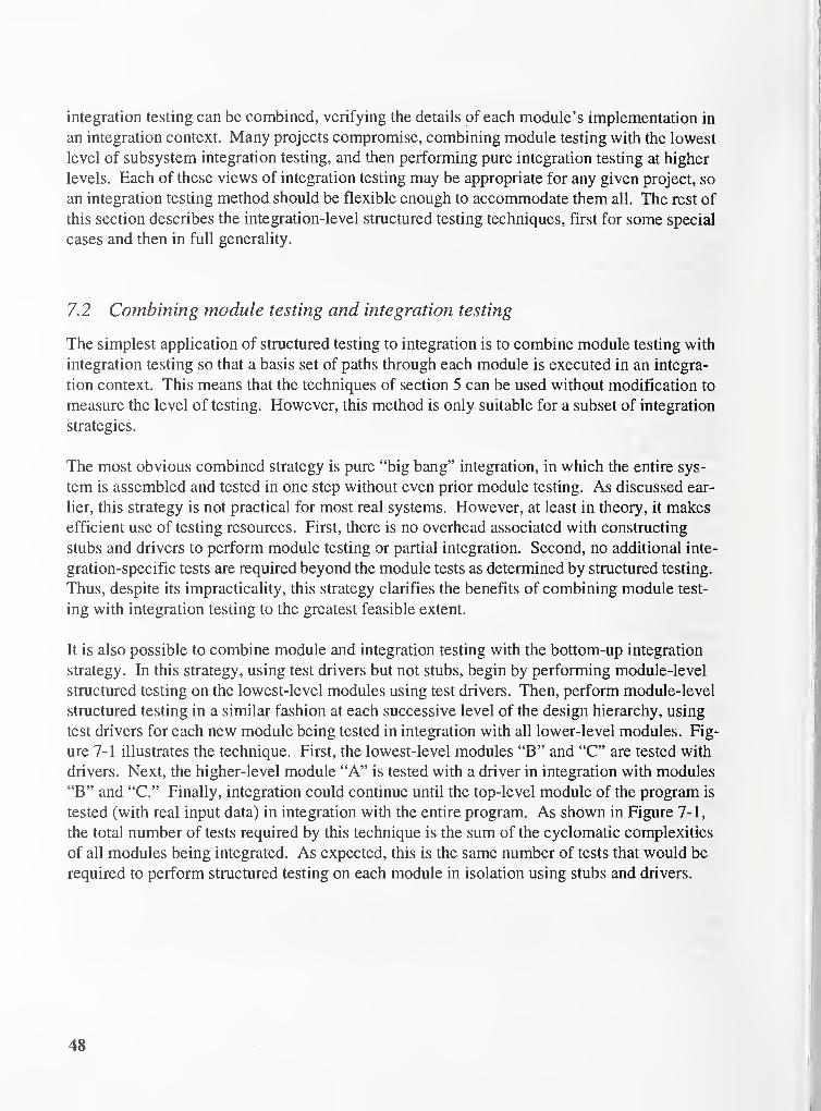
integration testing can be combined, verifying the details of each module's implementation in

an integration context. Many projects compromise, combining module testing with the lowest

level of subsystem integration testing, and then performing pure integration testing at higher

levels. Each of these views of integration testing may be appropriate for any given project, so

an integration testing method should be flexible enough to accommodate them all. The rest of

this section describes the integration-level structured testing techniques, first for some special

cases and then in full generality.

7.2 Combining module testing and integration testing

The simplest application of structured testing to integration is to combine module testing with

integration testing so that a basis set of paths through each module is executed in an integra-

tion context. This means that the techniques of section 5 can be used without modification to

measure the level of testing. However, this method is only suitable for a subset of integration

strategies.

The most obvious combined strategy is pure "big bang" integration, in which the entire sys-

tem is assembled and tested in one step without even prior module testing. As discussed ear-

lier, this strategy is not practical for most real systems. However, at least in theory, it makes

efficient use of testing resources. First, there is no overhead associated with constructing

stubs and drivers to perform module testing or partial integration. Second, no additional inte-

gration-specific tests are required beyond the module tests as determined by structured testing.

Thus, despite its impractical ity, this strategy clarifies the benefits of combining module test-

ing with integration testing to the greatest feasible extent.

It is also possible to combine module and integration testing with the bottom-up integration

strategy. In this strategy, using test drivers but not stubs, begin by performing module-level

structured testing on the lowest-level modules using test drivers. Then, perform module-level

structured testing in a similar fashion at each successive level of the design hierarchy, using

test drivers for each new module being tested in integration with all lower-level modules. Fig-

ure 7-1 illustrates the technique. First, the lowest-level modules "B" and "C" are tested with

drivers. Next, the higher-level module "A" is tested with a driver in integration with modules

"B" and "C." Finally, integration could continue until the top-level module of the program is

tested (with real input data) in integration with the entire program. As shown in Figure 7- 1

,

the total number of tests required by this technique is the sum of the cyclomatic complexities

of all modules being integrated. As expected, this is the same number of tests that would be

required to perform structured testing on each module in isolation using stubs and drivers.

48

Driver Driver DriverforB forC for A

B C A

Phase 1 : Test a basis set of

paths through B and C using

drivers. Number of tests is

v(B) + v(C).

Phase 2: Test a basis set of

paths through A in integration

with B and C using a driver.

Number of tests is v(A).

Total number of tests is v(A) + v(B) + v(C), the sum of the cyclomatic

complexities of all integrated modules.

Figure 7-1. Combining module testing with bottom-up integration.

73 Generalization ofmodule testing criteria

Module testing criteria can often be generalized in several possible ways to support integra-

tion testing. As discussed in the previous subsection, the most obvious generalization is to

satisfy the module testing criterion in an integration context, in effect using the entire program

as a test driver environment for each module. However, this trivial kind of generalization does

not take advantage of the differences between module and integration testing. Applying it to

each phase of a multi-phase integration strategy, for example, leads to an excessive amount of

redundant testing.

More useful generalizations adapt the module testing criterion to focus on interactions

between modules rather than attempting to test all of the details of each module's implementa-

tion in an integration context. The statement coverage module testing criterion, in which each

statement is required to be exercised during module testing, can be generalized to require each

module call statement to be exercised during integration testing. Although the specifics of the

generalization of structured testing are more detailed, the approach is the same. Since stnic-

49

tured testing at the module level requires that all the decision logic in a module's control flow

graph be tested independently, the appropriate generalization to the integration level requires

that just the decision logic involved with calls to other modules be tested independently. Thefollowing subsections explore this approach in detail.

7.4 Module design complexity

Rather than testing all decision outcomes within a module independently, structured testing at

the integration level focuses on the decision outcomes that are involved with module calls

[MCCABE2]. The design reduction technique helps identify those decision outcomes, so that

it is possible to exercise them independently during integration testing. The idea behind

design reduction is to start with a module control flow graph, remove all control structures

that are not involved with module calls, and then use the resultant "reduced" flow graph to

drive integration testing. Figure 7-2 shows a systematic set of rules for performing design

reduction. Although not strictly a reduction rule, the call rule states that function call ("black

dot") nodes cannot be reduced. The remaining rules work together to eliminate the parts of

the flow graph that are not involved with module calls. The sequential rule eliminates

sequences of non-call ("white dot") nodes. Since application of this rule removes one node

and one edge from the flow graph, it leaves the cyclomatic complexity unchanged. However,

it does simplify the graph so that the other rules can be applied. The repetitive rule eliminates

top-test loops that are not involved with module calls. The conditional rule eliminates condi-

tional statements that do not contain calls in their bodies. The looping rule eliminates bottom-

test loops that are not involved with module calls. It is important to preserve the module's

connectivity when using the looping rule, since for poorly-structured code it may be hard to

distinguish the "top" of the loop from the "bottom." For the rule to apply, there must be a

path from the module entry to the top of the loop and a path from the bottom of the loop to the

module exit. Since the repetitive, conditional, and looping rules each remove one edge from

the flow graph, they each reduce cyclomatic complexity by one.

50

Rules 1 through 4 are intended to be appHed iteratively until none of them can be applied, at

which point the design reduction is complete. By this process, even very complex logic can

be eliminated as long as it does not involve any module calls.

Rule 0: Call • •

Rule 1 : Sequential

Rule 2: Repetitive

Rule 3: Conditional

Rule 4: Looping

• = Call node O = Non-call node

® = Path of zero or more non-call nodes

= Any node, call or non-call

Figure 7-2. Design reduction rules.

Figure 7-3 shows a control flow graph before and after design reduction. Rules 3 and 4 can be

applied immediately to the original graph, yielding the intermediate graph. Then rule 1 can be

applied three times to the left conditional branch, at which point rule 3 can be applied again,

after which five more applications of rule 1 complete the reduction. The second application of

51

rule 3 illustrates that a conditional structure may be eliminated even if its body contains a call

node, as long as there is at least one path through its body that does not contain any call nodes.

Original graph, Intermediate graph, Reduced graph,

v(G) = 5 after rules 3 and 4 v(G) = 2have been applied

O = Non-call node # = Call node

Figure 7-3. Design reduction example.

The module design complexity, iv(G), is defined as the cyclomatic complexity of the reduced

graph after design reduction has been performed. In Figure 7-3, the module design complex-

ity is 2. The design flow graph in Figure 7-4 displays the logic that contributes to module

design complexity superimposed on the entire control flow graph for a module with cyclo-

matic complexity 6 and module design complexity 3.

52

,

;

!"

i7;:ii Flowgraphs for fjal analyze line' in 'prsftn'

;

1

i

Plot fSave] ConverT] [Forward|[Backward

|Enlarge Reduce Close Help

Page 1 of 1 2X

Program: prsftn 04/02/96 HFile: halstead. c Superimposed Bhal analpze line (J) upward Flows HLanguage: c Loop ExitsDesign Graph Plain Edges HCpclomatic 6 ^0 HEssentialIF B|Design 3 J i H

\ /^^""^ ^"^11* 1

\ \ \ i

\ 1^20* i

* inclicates call nocles|

'

r

"""— —.

..»-.."..»...,m,.I

Figure 7-4. Design graph with v(G) = 6, iv(G) = 3.

When structured testing has already been performed at the module level, module design com-

plexity can be used to drive integration testing, requiring a basis set of paths through each

module's reduced graph to be tested in integration. For the bottom-up integration strategy dis-

cussed in section 7-2, the total number of integration tests becomes the sum of the module

design complexities of all modules being integrated. Since module design complexity can be

significantly less than cyclomatic complexity, this technique reduces the number of integra-

tion tests. It also simplifies the process of deriving data for each test path, since there are

fewer constraints on paths through the reduced graph than on paths through the full graph.

53

7.5 Integration complexity

The integration complexity, Sj, is defined for a program with n modules (Gi through 0^) by

the formula: S| = (Z iv(Gj)) - n + 1 [MCCABE2]. Integration complexity measures the num-

ber of independent integration tests through an entire program's design. To understand the

formula, recall the baseline method of section 6 for generating a set of independent tests

through an individual module. The analogous integration-level method generates a set of

independent tests through the program's design. Begin with a baseline test, which contributes

1 to the Sj formula and exercises one path through the program's main module. Then, make

each successive test exercise exactly one new decision outcome in exactly one module's

design-reduced graph. Since the first "mini-baseline" path through each module comes as a

result of exercising a path in a higher-level module (except for the main module, which gets

its first path from the baseline test), each module contributes a number of new integration tests

equal to one less than its module design complexity, for a total contribution of Z (iv(Gi) - 1),

which (smce there are n modules) equals (E iv(Gi)) - n. Adding the 1 for the baseline test

gives the full Sj formula. A similar argument shows that substituting v(G) for iv(G) in the Sj

formula gives the number of tests necessary to test every decision outcome in the entire pro-

gram independently [FEGHALI].

Figure 7-5 shows an example program with integration complexity 4, giving the control struc-

ture, cyclomatic complexity, and module design complexity for each module and a set of four

independent integration tests.

54

v(A) = 2

iv(A) = 2

/

/

/

v(B) = 2

iv(B) = 2

/' /

\ /

\ /

\ i

\'

\ /

v(D) = 2

iv(D) = 1

v(C)

iv(C)

Si = (2 + 2 + 2+ 1) -4+ 1 = 4.

Independent integration tests:

LA2. A>B<A>C<A3. A>B>D<B<A>C<A4. A>B<A>C>D<C<AC'X > Y < X" means "X calls Y which returns to X.")

O = non-call node • = call node

Figure 7-5. Integration complexity example.

Although a basis set of paths through each module's design-reduced control flow graph can

typically be exercised with fewer than Sj integration tests, more tests are never required. For

the most rigorous level of structured testing, a complete basis set of S] integration tests should

be performed.

Integration complexity can be approximated from a structured design [YOURDON], allowing

integration test effort to be predicted before coding begins. The number of design predicates

in a structure chart (conditional and iterative calls) can be used to approximate the eventual

integration complexity. Recall the simplified formula for cyclomatic complexity from section

4. 1 , that for modules with only binary decisions and p decision predicates, v(G) = p + 1 . The

corresponding formula for integration complexity is that for programs with d design predi-

cates, Sj will be approximately d + 1 . The reason is that each design predicate (conditional or

iterative call) tends to be implemented by a decision predicate in the design-reduced graph of

a module in the eventual implemented program. Hence, recalling that iv(G) is the cyclomatic

complexity of the design-reduced graph, combine the v(G) and S j formulas to calculate the

approximation that Sj = I iv(G) - n + 1 = E (iv(G) - 1) + 1 = Z (v(GReduced) - 1) + 1 = d + 1,

where d is the total number of decision predicates in the design-reduced graphs of the modules

of the implemented program, and approximately equal to the number of design predicates in

the original program design. Figure 7-6 shows a structured design representation with three

design predicates and therefore an expected integration complexity of four.

A

* = design predicate (conditional call)

Since there are three design predicates,

The expected integration complexity is four.

Figure 7-6. Predicting integration complexity.

56

7.6 Incremental integration

Hierarchical system design limits each stage of development to a manageable effort, and it is

important to limit the corresponding stages of testing as well [WATSON5]. Hierarchical

design is most effective when the coupling among sibling components decreases as the com-ponent size increases, which simplifies the derivation of data sets that test interactions amongcomponents. The remainder of this section extends the integration testing techniques of struc-

tured testing to handle the general case of incremental integration, including support for hier-

archical design. The key principle is to test just the interaction among components at each

integration stage, avoiding redundant testing of previously integrated sub-components.

As a simple example of the approach, recall the statement coverage module testing criterion

and its integration-level variant from section 7.2 that all module call statements should be

exercised during integration. Although this criterion is certainly not as rigorous as structured

testing, its simplicity makes it easy to extend to support incremental integration. Although the

generalization of structured testing is niore detailed, the basic approach is the same. To extend

statement coverage to support incremental integration, it is required that all module call state-

ments from one component into a different component be exercised at each integration stage.

To form a completely flexible "statement testing" criterion, it is required that each statement

be executed during the first phase (which may be anything from single modules to the entire

program), and that at each integration phase all call statements that cross the boundaries of

previously integrated components are tested. Given hierarchical integration stages with good

cohesive partitioning properties, this limits the testing effort to a small fraction of the effort to

cover each statement of the system at each integration phase.

Structured testing can be extended to cover the fully general case of incremental integration in

a similar manner. The key is to perform design reduction at each integration phase using just

the module call nodes that cross component boundaries, yielding component-reduced graphs,

and exclude from consideration all modules that do not contain any cross-component calls.

Integration tests are derived from the reduced graphs using the techniques of sections 7.4 and

7.5. The complete testing method is to test a basis set of paths through each module at the first

phase (which can be either single modules, subsystems, or the entire program, depending on

the underlying integration strategy), and then test a basis set of paths through each compo-

nent-reduced graph at each successive integration phase. As discussed in section 7.5, the most

rigorous approach is to execute a complete basis set of component integration tests at each

stage. However, for incremental integration, the integration complexity formula may not give

the precise number of independent tests. The reason is that the modules with cross-compo-

nent calls may not be connected in the design structure, so it is not necessarily the case that

one path through each module is a result of exercising a path in its caller. However, at most

one additional test per module is required, so using the S \ formula still gives a reasonable

approximation to the testing effort at each phase.

57

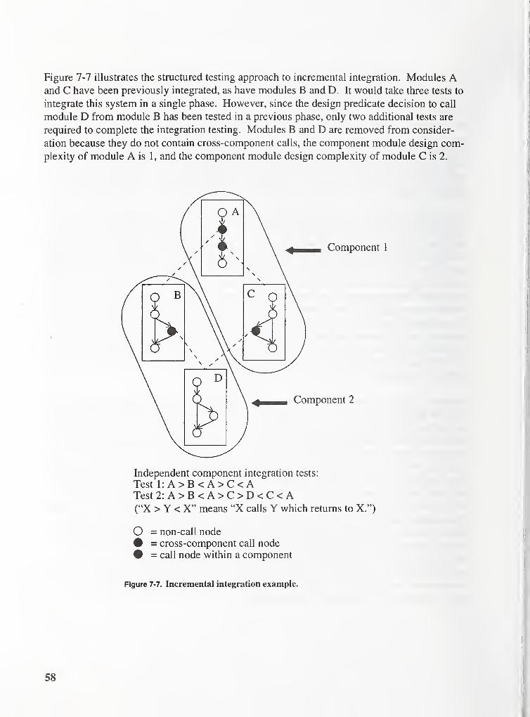
Figure 7-7 illustrates the structured testing approach to incremental integration. Modules Aand C have been previously integrated, as have modules B and D. It would take three tests to

integrate this system in a single phase. However, since the design predicate decision to call

module D from module B has been tested in a previous phase, only two additional tests are

required to complete the integration testing. Modules B and D are removed from consider-

ation because they do not contain cross-component calls, the component module design com-

plexity of module A is 1, and the component module design complexity of module C is 2.

Independent component integration tests:

Test 1:A>B<A>C<ATest 2:A>B<A>C>D<C<A("X > Y < X" means "X calls Y which returns to X.")

O = non-call node

# = cross-component call node

# = call node within a component

Figure 7-7. Incremental integration example.

58

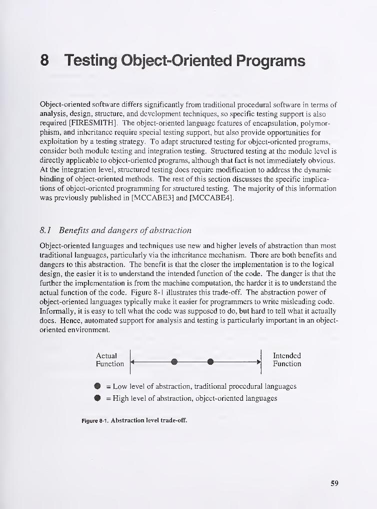
8 Testing Object-Oriented Programs

Object-oriented software differs significantly from traditional procedural software in terms of

analysis, design, structure, and development techniques, so specific testing support is also

required [FIRESMITH]. The object-oriented language features of encapsulation, polymor-

phism, and inheritance require special testing support, but also provide opportunities for

exploitation by a testing strategy. To adapt structured testing for object-oriented programs,

consider both module testing and integration testing. Structured testing at the module level is

directly applicable to object-oriented programs, although that fact is not immediately obvious.

At the integration level, structured testing does require modification to address the dynamic

binding of object-oriented methods. The rest of this section discusses the specific implica-

tions of object-oriented programming for structured testing. The majority of this information

was previously published in [MCCABE3] and [MCCABE4].

8.1 Benefits and dangers ofabstraction

Object-oriented languages and techniques use new and higher levels of abstraction than most

traditional languages, particularly via the inheritance mechanism. There are both benefits and

dangers to this abstraction. The benefit is that the closer the implementation is to the logical

design, the easier it is to understand the intended function of the code. The danger is that the

further the implementation is from the machine computation, the harder it is to understand the

actual function of the code. Figure 8-1 illustrates this trade-off. The abstraction power of

object-oriented languages typically make it easier for programmers to write misleading code.

Informally, it is easy to tell what the code was supposed to do, but hard to tell what it actually

does. Hence, automated support for analysis and testing is particularly important in an object-

oriented environment.

Actual

Function

Intended

Function

= Low level of abstraction, traditional procedural languages

= High level of abstraction, object-oriented languages

Figure 8-1. Abstraction level trade-off.

59

When abstraction works well, it hides details that do not need to be tested, so testing becomes

easier. When abstraction works poorly, it hides details that need to be tested, so testing

becomes harder (or at worst, infeasible). Typically, testing must occur at some compromise

level of abstraction, gaining leverage from the abstractions that clarify the software's func-

tionality while penetrating the abstractions that obscure it. Often, a software developer's level

of familiarity with object-oriented development techniques is a key factor in determining

whether abstraction is used in a positive or negative way, which in turn determines whether

testing is helped or hindered by the unique features of object-oriented languages. As dis-

cussed in section 8-3, the basic object-oriented structured testing approach can be adapted to

unusually positive or negative situations.

Metrics designed specifically for object-oriented software, such as those of [CHIDAMBER],can help assess the effectiveness with which the object-oriented paradigm is used. If class

methods are not cohesive and there is substantial coupling between objects, the abstractions of

the programming language may have been misused in the software. This in turn suggests that

extra caution should be taken during testing.

8.2 Object-oriented module testing

Object-oriented methods are similar in most respects to ordinary functions, so structured test-

ing (as well as other structural testing criteria) applies at the module level without modifica-

tion. Since methods in object-oriented languages tend to be less complex than the functions of

traditional procedural programs, module testing is typically easier for object-oriented pro-

grams.

The inheritance and polymorphism features of object-oriented languages may seem to compli-

cate module testing, because of the implicit control flow involved in resolving dynamic

method invocations. For example, if an object reference could result in any one of several

alternative methods being executed at run time, it is possible to represent the reference as a

multi-way decision construct ("case" statement) on the flow graph in which a different possi-

ble resolution method for the object reference is called from each branch. Since this represen-

tation of implicit control flow would increase the cyclomatic complexity, it would also

increase the number of tests required to perform structured testing for the module containing

the reference. Figure 8-2 illustrates implicit control flow.

60

Object reference

M, showingimplicit

control flow

/

/ I

'A

Resolution 1

/^\ /

Reso/ution 2 Resolution 3

Figure 8-2. Implicit control flow.

Although implicit control flow has significant implications for testing, there are strong rea-

sons to ignore it at the level of module testing. First, the number of possible resolutions of a

particular object reference depends on the class hierarchy in which the reference occurs.

Hence, if module testing depended on implicit control flow, it would only be possible to per-

form module testing in the context of a complete class hierarchy, a clearly unrealistic require-

ment. Also, viewing implicit complexity as a module property rather than a system property

defeats one of the major motivations for using an object-oriented language: to develop easily

reusable and extensible components. For these reasons, consideration of implicit control flow

is deferred until the integration phase when applying structured testing to object-oriented pro-

grams.

8.3 Integration testing of object-orientedprograms

The most basic application of structured testing to the integration of object-oriented programs

is essentially the direct application of the techniques of section 7. It is vitally important, how-

ever, to consider the implicit method invocations through object references (not to be con-

fused with the implicit control flow of dynamic binding) when identifying function call nodes

to perform design reduction. These method invocations may not be apparent from examina-

tion of the source code, so an automated tool is helpful. For example, if variables "a" and "b"

are integers, the C+-i- expression "a+b" is a simple computation. However, if those variables

61

are objects of a class type, the exact same expression can be a call to a method of that class via

the operator overloading mechanism of C++, which requires integration testing and hence

must be preserved by design reduction.

While the treatment of implicit method calls due to object references is straightforward, the

situation with implicit control flow is more complicated. In this case, several possible

approaches are worth considering, depending on the extent to which the object-oriented

abstraction has a positive or negative impact. This section describes three approaches: opti-

mistic, pessimistic, and balanced. Each approach builds upon the techniques of section 7,

requiring that at least a basis set of tests through the design-reduced graph of each module be

exercised in an integration context, treating the implicit method invocations due to object ref-

erences as calls when performing design reduction. The pessimistic and balanced approaches

also require additional tests based on implicit control flow. Figure 8-3 shows the structure of

a small subset of a program that illustrates each approach. Each of modules "A," "B," and

"C" invokes the dynamically bound "Draw" method, which can be resolved at run time to any

of "Line::Draw," "Polygon: :Draw," and "Ellipse: :Draw." For the rest of this section, the

methods that may be invoked as a result of a dynamically bound object reference will be

referred to as "resolutions."

A B C

Draw

Line::Draw Polygon: :Draw Ellipse::Draw

Figure 8-3. Implicit control flow example.

The optimistic approach is the most straightforward integration testing approach. With this

approach, it is expected that abstraction will have a positive impact, and therefore testing will

be confined to the level of abstraction of the source code. The integration testing techniques

of section 7 apply directly. The consequences for implicit control flow are that each call site

exercises at least one resolution, and each resolution is exercised by at least one call site.

Assuming that no errors are uncovered by testing those interfaces, the object-oriented abstrac-

tion is trusted to gain confidence that the other possible interfaces are also correct. Figure 8-4

shows a set of interface tests that are adequate to satisfy the optimistic approach for the exam-

ple of Figure 8-3.

62

Figure 8-4. The optimistic approach to implicit control flow.

The pessimistic approach is another fairly straightforward approach. With this approach,

abstraction is expected to have a negative impact, and therefore testing is required at the level

of abstraction of the machine computation underlying the source code. In addition to the inte-

gration testing techniques of section 7, implicit control flow is tested by requiring that every

resolution be tested from every call site. Thus, each interface is tested directly, and no trust is

placed in the object-oriented abstraction. The drawback is that the testing effort can quickly

become infeasible as complexity increases. Figure 8-5 shows a set of interface tests that are

adequate to satisfy the pessimistic approach for the example of Figure 8-3.

A B C

Line::Draw Polygon ::Draw Ellipse: :Draw

Figure 8-5. The pessimistic approach to implicit control flow.

The balanced approach is a compromise between the optimistic and pessimistic approaches,

and is more complicated than either of them. The idea is to test at a level of abstraction

between that of the code and that of the underlying mechanics. Abstraction is expected to

hide some details that require testing, but also to provide a framework that can be exploited to

facilitate testing. In addition to the integration testing techniques of section 7, it is required

that some call site exercise the entire set of possible resolutions. The effect of this require-

63

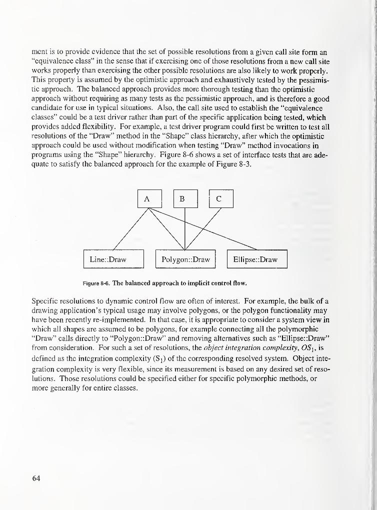
ment is to provide evidence that the set of possible resolutions from a given call site form an

"equivalence class" in the sense that if exercising one of those resolutions from a new call site

works properly than exercising the other possible resolutions are also likely to work properly.

This property is assumed by the optimistic approach and exhaustively tested by the pessimis-

tic approach. The balanced approach provides more thorough testing than the optimistic

approach without requiring as many tests as the pessimistic approach, and is therefore a goodcandidate for use in typical situations. Also, the call site used to establish the "equivalence

classes" could be a test driver rather than part of the specific application being tested, which

provides added flexibility. For example, a test driver program could first be written to test all

resolutions of the "Draw" method in the "Shape" class hierarchy, after which the optimistic

approach could be used without modification when testing "Draw" method invocations in

programs using the "Shape" hierarchy. Figure 8-6 shows a set of interface tests that are ade-

quate to satisfy the balanced approach for the example of Figure 8-3.

Figure 8-6. The balanced approach to implicit control flow.

Specific resolutions to dynamic control flow are often of interest. For example, the bulk of a

drawing application's typical usage may involve polygons, or the polygon functionality mayhave been recently re-implemented. In that case, it is appropriate to consider a system view in

which all shapes are assumed to be polygons, for example connecting all the polymorphic

"Draw" calls directly to "Polygon: :Draw" and removing alternatives such as "Ellipse: :Draw"

from consideration. For such a set of resolutions, the object integration complexity, OSi, is

defined as the integration complexity (Sj) of the corresponding resolved system. Object inte-

gration complexity is very flexible, since its measurement is based on any desired set of reso-

lutions. Those resolutions could be specified either for specific polymorphic methods, or

more generally for entire classes.

64

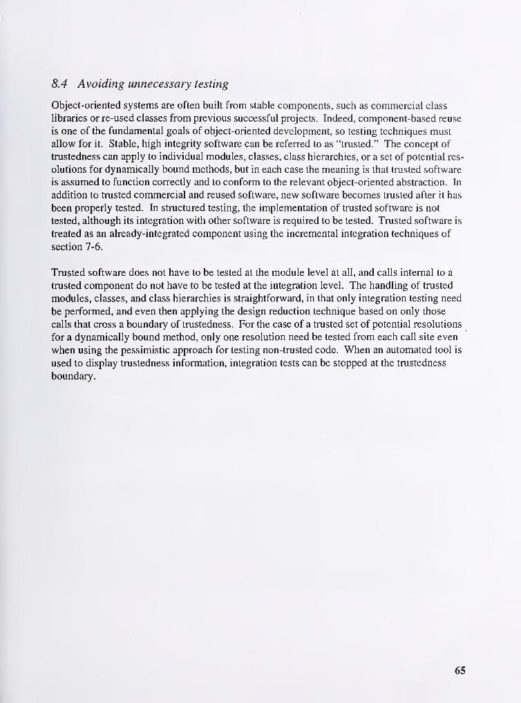
8.4 Avoiding unnecessary testing

Object-oriented systems are often built from stable components, such as commercial class

libraries or re-used classes from previous successful projects. Indeed, component-based reuse

is one of the fundamental goals of object-oriented development, so testing techniques must

allow for it. Stable, high integrity software can be referred to as "trusted." The concept of

trustedness can apply to individual modules, classes, class hierarchies, or a set of potential res-

olutions for dynamically bound methods, but in each case the meaning is that trusted software

is assumed to function correctly and to conform to the relevant object-oriented abstraction. In

addition to trusted commercial and reused software, new software becomes trusted after it has

been properly tested. In structured testing, the implementation of trusted software is not

tested, although its integration with other software is required to be tested. Trusted software is

treated as an already-integrated component using the incremental integration techniques of

section 7-6.

Trusted software does not have to be tested at the module level at all, and calls internal to a

trusted component do not have to be tested at the integration level. The handling of trusted

modules, classes, and class hierarchies is straightforward, in that only integration testing need

be performed, and even then applying the design reduction technique based on only those

calls that cross a boundary of trustedness. For the case of a trusted set of potential resolutions

for a dynamically bound method, only one resolution need be tested from each call site even

when using the pessimistic approach for testing non-trusted code. When an automated tool is

used to display trustedness information, integration tests can be stopped at the trustedness

boundary.

65

I

1

I.

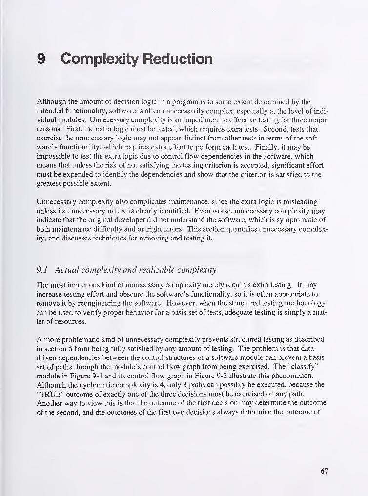
9 Complexity Reduction

Although the amount of decision logic in a program is to some extent determined by the

intended functionality, software is often unnecessarily complex, especially at the level of indi-

vidual modules. Unnecessary complexity is an impediment to effective testing for three major

reasons. First, the extra logic must be tested, which requires extra tests. Second, tests that

exercise the unnecessary logic may not appear distinct from other tests in terms of the soft-

ware's functionality, which requires extra effort to perform each test. Finally, it may be

impossible to test the extra logic due to control flow dependencies in the software, which

means that unless the risk of not satisfying the testing criterion is accepted, significant effort

must be expended to identify the dependencies and show that the criterion is satisfied to the

greatest possible extent.

Unnecessary complexity also complicates maintenance, since the extra logic is misleading

unless its unnecessary nature is clearly identified. Even worse, unnecessary complexity mayindicate that the original developer did not understand the software, which is symptomatic of

both maintenance difficulty and outright errors. This section quantifies unnecessary complex-

ity, and discusses techniques for removing and testing it.

9.1 Actual complexity and realizable complexity

The most innocuous kind of unnecessary complexity merely requires extra testing. It mayincrease testing effort and obscure the software's functionality, so it is often appropriate to

remove it by reengineering the software. However, when the structured testing methodology

can be used to verify proper behavior for a basis set of tests, adequate testing is simply a mat-

ter of resources.

A more problematic kind of unnecessary complexity prevents structured testing as described

in section 5 from being fully satisfied by any amount of testing. The problem is that data-

driven dependencies between the control structures of a software module can prevent a basis

set of paths through the module's control flow graph from being exercised. The "classify"

module in Figure 9-1 and its control flow graph in Figure 9-2 illustrate this phenomenon.

Although the cyclomatic complexity is 4, only 3 paths can possibly be executed, because the

"TRUE" outcome of exactly one of the three decisions must be exercised on any path.

Another way to view this is that the outcome of the first decision may determine the outcome

of the second, and the outcomes of the first two decisions always determine the outcome of

67

the third. Figures 9-3 and 9-4 show "classify2," a reengineered version with no unnecessary

complexity.

jPrint

IjSave| [corwrt] [cTose] [Help]


Program : ClassifyFile : classify.Language: c_nppModule ModuleLetter Name

04/09/96

& classify

AO

AlA2A3 A4ASA6 A7A8A9 AlO


4 1 4

void classify (int n){/* Example of unnecessary complexity */

if (n > 0)printf( "Posit ive\n" )

;

if (n < 0)printf ( "Negat ive\n" )

;

if (n 0)printf ( "Zero\n" )

;

)

Figure 9-1 . Code for module with unnecessary complexity.

JassHy'tn'Otasliy

[pTot] [Eave] [Corr<ert| fForwd| [Backuard| jinfa-gel j Reduce] [cicise] [fielp]

Page 1 of 1 2X

laasify. cclassiry (A)Laxiauagfe ; c

'

CyclomatxcCycLomatic^Essential 1Design 4

04AI9/96Superiiaopsed..pipvarg Flovs

—

Loop ExitsPlain Edges

—

Figure 9-2. Graph for module with unnecessary complexity.

68

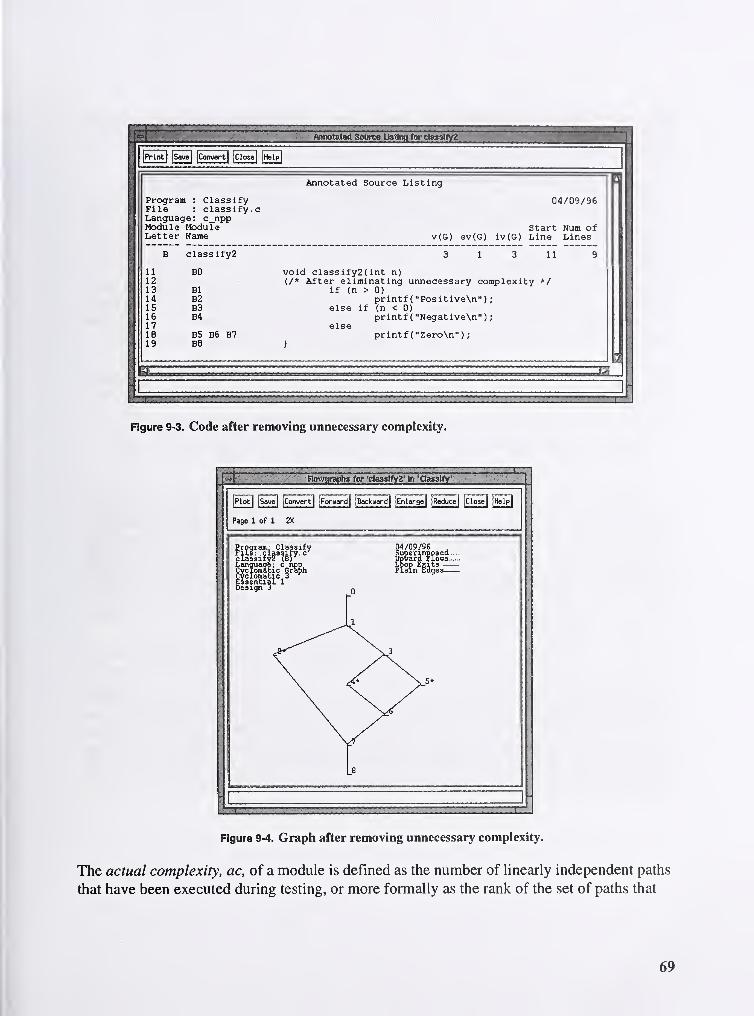
IPrinT] fsave| |Convert|[cTose] jHelp]


ProgramFileLanguage _Module [toduleLetter Name

Classifyclassify .

c

c_npp

04/09/96

B classify2

11 BO1213 Bl14 B215 B316 B41718 B5 B6 B719 B8


1 11

void classify2 ( int n){/* After eliminating unnecessary complexity */

if (n > 0)printf ("PositiveXn")

;

else if (n < G)printf ( "Negative\n" )

;

elseprintf ( "ZeroXn" )

;

mm

Figure 9-3. Code after removing unnecessary complexity.

Figure 9-4. Graph after removing unnecessary complexity.

The actual complexity, ac, of a module is defined as the number of Hnearly independent paths

that have been executed during testing, or more formally as the rank of the set of paths that

69

have been executed during testing. The structured testing criterion requires that the actual

complexity equal the cyclomatic complexity after testing. Note that the actual complexity is a

property of both the module and the testing. For example, each new independent test

increases the actual complexity.

The realizable complexity, rc, is the maximum possible actual complexity, i.e., the rank of the

set of the paths induced by all possible tests. This is similar to the characterization of cyclo-

matic complexity as the rank of the set of all possible paths, except that some paths may not be

induced by any test. In the "classify" example, rc is 3 whereas v(G) is 4. Although rc is an

objective and well-defined metric, it may be hard to calculate. In fact, calculating rc is theo-

retically undecidable [HOPCROFT], since, if it were possible to calculate rc, it would also be

possible to determine whether rc is at least 1 , which would indicate whether at least one com-

plete path could be executed, which is equivalent to the module halting on some input.

One obvious property of rc is that after any amount of testing has been performed on a mod-

ule, ac <= rc <= v(G). Satisfying the structured testing criterion therefore suffices to prove

that rc = v(G). However, when ac < v(G), one of two situations can hold:

1. At least one additional independent test can be executed.

2. ac = rc, and hence rc < v(G).

In the first case, the solution is simply to continue testing until either ac = v(G) or case 2 is

reached. In the second case, the software can typically be reengineered to remove unneces-

sary complexity, yielding a module in which rc = v(G). This was performed in the "classify"

example. As an alternative to reengineering the software, the structured testing criterion can

be modified to require testing until ac = rc. However, due to the undecidability of rc, some

manual work is required to set the target value when using an automated tool to measure ac.

A tool can help by reporting the current set of control dependencies, at which point the user

can review the observed dependencies and decide whether or not additional tests could

increase ac. If additional tests can increase ac, dependency information can also help con-

struct those tests. One special case is "infinite loop" modules, which have rc = 0 because no

complete path can be executed. This does not mean that these modules should not be tested at

all! Infinite loops in real software are typically not really infinite, they are just waiting for

some external event to interrupt them in a way that is not explicitly specified in their source

code. Such modules should be as small as possible, so that they can be adequately tested just

by executing them once. Any complex processing should be performed by subordinate mod-

ules that do not contain infinite loops, and hence have basis paths to test.

70

There are many situations in which it is easy to see that re < v(G). One example is a loop with

a constant number of iterations, such as the "min" module in Figure 9-5. The "TRUE" out-

= Annotatod Sourca listing for win . ^•

1Print

1

jSave] (Convert|jciosej |Help|


Program : Dep 04/09/96File : dep.cLanguage: c_nppModule Module Start Num ofLetter Name v(G) ev(G) iv(G) Line Lines

B min 3 11 3 9

3 BO int min ( int a[10]

)

4 (/* reads array of ten elements and returns the smallest */5 int i, result;6 result = a[0]

;

I Bl B2 for (i - 0; i < 10; i++)8 B3 if (result > a[i]

)

9 B4 result - a[i];10 B5 B6 return result;II B7 )

A

./

^ II 1 11.11 1. .1.^

Figure 9-5. Loop with constant number of iterations.

come of the loop is always executed ten times as frequently as the "ENTRY" branch along

any executable path, which is a linear control dependency and thus reduces rc by one. Loops

with a constant number of iterations are fairly common in software. When the constant might

change during maintenance (for example, a hash table size), it is worth running a test with a

different constant value. When the constant will not change (for example, the number of axes

in graphics rendering code), the dependency can simply be taken into account during testing.

9.2 Removing control dependencies

Removing control dependencies often improves code, since the resulting modules tend to be

less complex and have straightforward decision logic. When all dependencies are removed,

testing is facilitated by allowing the cyclomatic complexity to be used as a target for actual

complexity. Two important reduction techniques are direct logic simplification and modular-

ization. The following complex example [WATS0N5] illustrates both techniques. Figure 9-

6 shows the code for module "printwords," [HANSON] which contains three control depen-

71

dencies (for this example, HASHSIZE is not constant). One dependency is the "&& k~ > 0"

^otetetf Source ttetln^ forprtntwoms i

jPrintl fSave) jConvert| fciose] fHelT]


Program : Printwords 04/09/96File : printwords.

c

Language : c_nppModule Module Start Num ofLetter Name v(G) ev(G) iv(G) Line Lines

D printwords 11 3 2 32 22

32 DO printwords ( k)33 int k;34 (/* Print the k most common words in the table, original */35 int i, max;

struct word *wp, **list, *q;3637 max - 0;38 Dl 02 for (i = 0; i <= HASHSIZE; i++)39 D3 04 D5 for (wp - hashtable[ i] ; wp; wp = wp->next)40 D6 if (wp->count > max)41 D7 max = wp->count

;

42 D8 D9 DIO Oil list " (struct word **) alloc(max + 1, sizeof wp)

;

43 D12 013 for (i = 0; i <= HASHSIZE; i++)44 D14 015 016 for (wp = hashtable[ i] ; wp; wp = q) {

45 017 q = wp->next;46 wp->next = 1 ist [wp->count ]

;

47 018 1 ist [wp->count ] - wp;)48 019 D20

49 021 022 023 for (i = max; i >= 0 «£ k > 0; i—

)

50 024 D25 if ((wp = list[i]) <;s k— > 0)51 D26 027 028 for ( ; wp; wp = wp->next)

printf("%d %s\n", wp->count, wp->word)

;

52 029 O30 03153 032 033 034 )

ijmuuinm.ii.ji»jiiiimumiM)juuii»iJ»JLimurouiu.uuiujJ^u^^^

Figure 9-6. Module with three dependencies.

condition at line 50. This condition is always true, since it can only be reached when "k > 0"

is true at line 49, and the value of k is not changed in the interim. The condition can therefore

be eliminated, moving the "k~" to the initialization part of the loop on line 5 1 to preserve

functionality. The other two dependencies are due to the hash table being traversed twice,

once to get the value of "max" for the list allocation, then again to fill the list. These depen-

dencies can be eliminated by modularization of the "max" calculation. Figures 9-7 and 9-8

72

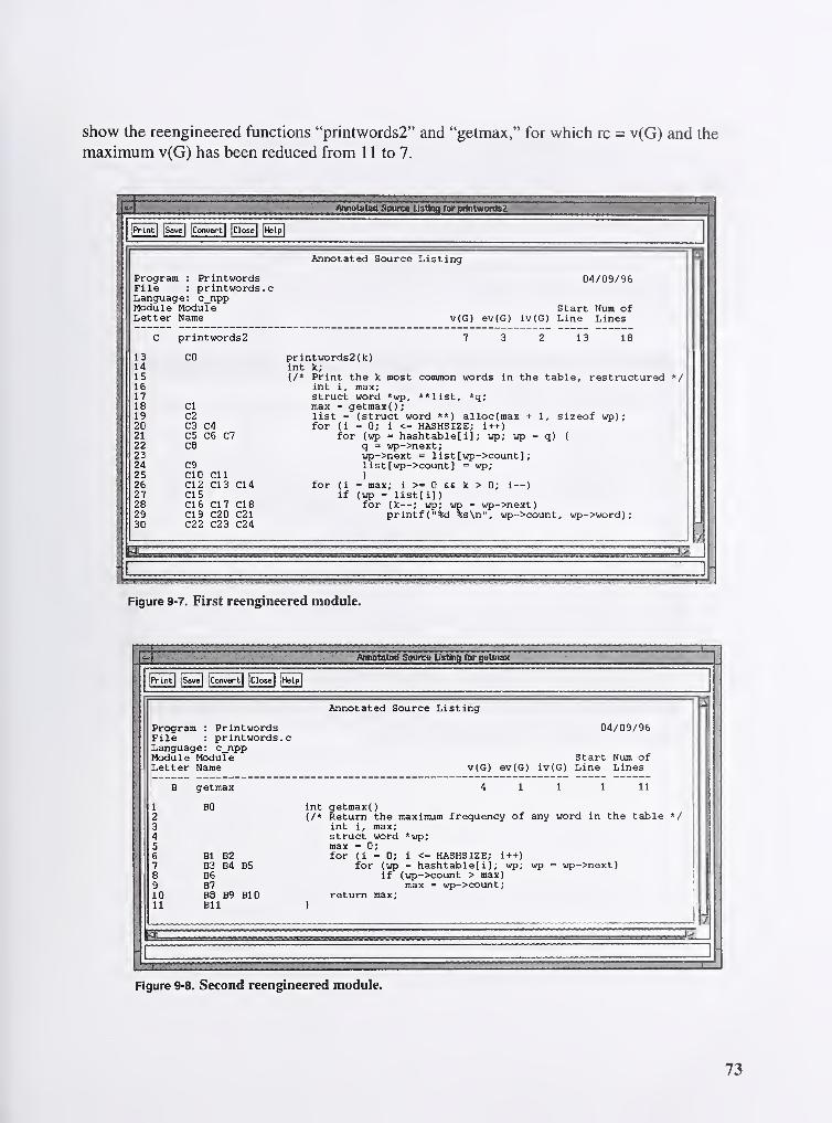
show the reengineered functions "printwords2" and "getmax," for which rc = v(G) and the

maximum v(G) has been reduced from 11 to 7.

/Vinetatetl Source listing for tirtntwontsz

iPrVnt] fSaue] jConvert] jcTosel [Help]


Program : PrintwordsFile : printwords.

c

Language: c_nppModule ModuleLetter Name

04/09/96


printwords2

CO

CIC2C3 C4C5 C6 C7C8

C9CIO CllCI 2 CI 3 CI 4

CISCI 6 CI 7 CI 8

CI 9 C20 C21C22 C23 C24

13 18

printwords2()c)int k;(/* Print the k most common words in the table, restructured */

int i, max;struct word *wp, **list, *q;max = getmax ( )

;

list = (struct word **) alloc(max + 1, sizeof wp)

;

for (i = 0; i <= HASHSIZE; i++)for (wp = hashtable[ i ] ; wp; wp = q) {

q = wp->next;wp->next = list [wp->count ]

;

1 ist [wp->count ] = wp;)

for (i = max; i >- 0 Sfi k > 0; i—

)

if (wp = list[i]

)

for (k— ; wp; wp = wp->next)printf("%d %s\n", wp->count, wp->word);

Figure 9-7. First reengineered module.

/Annotated! Source listing for getoiax

|Print| jSavej [Convert| iClose] ^Help


ProgramFileLanguage : c_nppModule ModuleLetter Name

Printwordsprintwords .

c

04/09/96

1

234567891011

B getmax

BO

Bl B2B3 B4 BSB6B7B8 39 BIOBll


4 11 1 11

int getmax ()

{/* Return the maximum frequency of any word in the table */int i, max;struct word *wp;max = 0;for (i = 0; i <- HASHSIZE; i++)

for (wp = hashtable[ i] ; wp; wp = wp->next)if (wp->count > max)

max = wp->count;return max;

>

Figure 9-8. Second reengineered module.

9.3 Trade-offs when reducing complexity

Removing control dependencies, although typically beneficial, can sometimes have a negative

impact on software. The most common pitfall when reducing complexity is to introduce

unstructured logic. The essential complexity metric, described in section 10, can help resolve

this problem by quantifying unstructured logic. However, structural degradation is often

obvious directly from the code and flow graph. Figures 9-9 and 9-10 show the code and graph

for "search," a well-structured module with v(G) = 4 and rc = 3. This type of code is often

seen in Pascal programs, using a single Boolean to control a loop and assigning it a value

based on multiple termination conditions.

Annotated Source Usting for search]

jPrlnt| [Save] fcotiwert) [ciosej [fielp]|

Annotated Source Listing|

Program : Tradeoff 04/10/96\

File : tradeoff.

c

Language : c_npp|

Module Module Start Num ofLetter Name vCG) ev(G) iv(G) Line Lines

B search 4 1 1 1 14

1 BO int search (char s[], int ch)2 (

3 int i, fDone, fFound;4 i = fDone = fFound = 0;5 Bl while (! fDone) {

6 B2 if (s[i] == ch) {

7 B3 fDone = 1

;

8 fFound = 1

;

9 B4 ) else if (s[i] == '\0')10 B5 fDone = 1;11 B6 B7 B8 i++;12 B9 )

13 return fFound;14 BIO )

IF

1

1

Figure 9-9. Code for structured module, rc < v(G).

74

nowgraphs for 'saarch' In Traiteoff

[Plot] [saveI[convert! [poruard! |iackuard! [Enlygel [Reduce] [cl^ |Help|

Page 1 of 1 2X

Figure 9-10.Graph for structured module, rc < v(G).

Figures 9-1 1 and 9-12 show the code and graph for a reengineered version of the same mod-

ule, with rc and v(G) both equal to 3. Although in principle this is an improvement, the new

version is not well-structured. The loop has two exit points, the bottom test and the condi-

tional return in the middle. Even so, most programmers would agree that the reengineered

version is better in this simple example. However, for more complex programs the structural

degradation from complexity reduction can be much more severe, in which case the original

version would be preferred. There is also a "middle ground" of programs for which reason-

able programmers can disagree about the desirability of reengineering, depending on their

75

experience and stylistic preferences. In such cases, it is less important to worry about making

the "right" choice, and more important to document the reasons for the trade-off.

[Prlntl ISave] fconvert| iClose| ;Help|


ProgramFileLanguage _Module ModuleLetter Name

Tradeofftradeoff

.

c npp

04/10/96


search2 16 10

16 CO17181920 Cl21 C222 C323 C4 C5 C62425 C7

int search2(char s[], int ch){

int i;

i = 0;do {

if (s[i] == ch)return 1

;

) while (s[i++]);return 0;

)

Figure 9-1 1 .Reengineered code, rc = v(G) but not well-structured.

Figure 9-12.Reengineered graph, v(G) = rc but not well-structured.

76

In addition to the trade-off between direct complexity reduction and structural quality, there is

also a trade-off between modularization and design quality [PARNAS]. When splitting a con-

trol dependency across a module boundary, there is the risk of introducing control coupling

between the modules and limiting the cohesion of each module. As when considering split-

ting up a module to satisfy a complexity threshold, the most important consideration is

whether each new module performs a single cohesive function. If it does, then the modular-

ization is consistent with design quality. Otherwise, the design quality degradation must be

weighed against the benefits of the reduced complexity. In the "printwords" example, the

new "getmax" function performed a single cohesive function, so the complexity reduction

was justified. If, on the other hand, the module was split in such a way as to require passing

local variables by reference and the only name that could be thought of for the new module

was "more_printwords," the modularization would not have been justified. As with structural

quality, having a clearly documented reasoning process is vital when the trade-off seems

fairly balanced.

77

1 0 Essential Complexity

In addition to the quantity of decision logic as measured by cyclomatic complexity, the quality

of that logic is also a significant factor in software development [PRESSMAN]. Structured

programming [DAHL] avoids unmaintainable "spaghetti code" by restricting the usage of

control structures to those that are easily analyzed and decomposed. Most programming lan-

guages allow unstructured logic, and few real programs consist entirely of perfectly structured

code. The essential complexity metric described in this section quantifies the extent to which

software is unstructured, providing a continuous range of structural quality assessments appli-

cable to all software rather than the "all or nothing" approach of pure structured programming.

10.1 Structured programming and maintainability

The primitive operations of structured programming, shown in Figure 10-1, are sequence,

selection, and iteration.

"if "case" "while" "repeat"

Sequence Selection Iteration

Figure 10-1 .Structured programming primitives.

The fundamental strength of structured programming is that the primitive operations give a

natural decomposition of arbitrarily complex structures. This decomposition facilitates modu-

larization of software because each primitive construct appears as a component with one entry

point and one exit point. The decomposition also allows a "divide and conquer" strategy to be

used to understand and maintain complex software even when the software is not physically

decomposed. Unstructured code must typically be understood and maintained as a single unit,

which can be impractical even for programs of moderate cyclomatic complexity.

Since poor module structure makes software harder to understand, it also impedes testing.

First, as discussed in section 5.3, poorly understood software requires extra testing to gain

confidence. Second, it requires more effort to construct each specific test case for poorly

79

understood code, since the connection between input data and the details of the implementa-

tion tends to be unclear. Finally, poorly understood code is both error-prone and hard to

debug, so an iterative process of testing and error correction may be required.

10.2 Definition of essential complexity, ev(G)

The essential complexity, ev(G) [MCCABEl], of a module is calculated by first removing

structured programming primitives from the module's control flow graph until the graph can-

not be reduced any further, and then calculating the cyclomatic complexity of the reduced

graph. An immediate consequence is that 1 <= ev(G) <= v(G). A somewhat less obvious con-

sequence, which can help when evaluating complexity analysis tools, is that ev(G) can never

be equal to 2. This is because after all sequential nodes have been eliminated, the only graphs

with v(G) equal to 2 are structured programming primitives, which can then be removed to get

an ev(G) of 1 . The reduction proceeds from the deepest level of nesting outward, which

means that a primitive construct can be removed only when no other constructs are nested

within it.

It is important to note that the structured programming primitives used in the calculation of

essential complexity are based on the control flow graph rather than the source code text. This

allows the essential complexity metric to measure structural quality independently of the syn-

tax of any particular programming language. For example, a bottom-test loop is a structured

primitive whether it is written using a high-level looping construct or an assembly language

conditional branch. Programming language constructs such as the "goto" statement only

increase essential complexity when they are actually used to implement poorly structured

logic, not just because they could be used that way. Of course, any program that is written

entirely with high-level "structured programming" language constructs will have a perfectly

structured control flow graph and therefore have an essential complexity of 1

.

The essential complexity calculation process is similar to the calculation of module design

complexity as described in section 7.4 (and in fact was developed first), but there are two key

differences. First, primitive constructs can be removed whether or not they involve module

calls when calculating essential complexity. Second, only entire primitive constructs can be

removed when calculating essential complexity. The module design complexity reduction

rules allow removing partial decision constructs when there are no module calls involved,

which can eliminate unstructured code. Thus, despite the similarity between the two calcula-

tion methods, there is no mathematical relationship between the two metrics.

80

10.3 Examples of essential complexity

Figure 10-2 illustrates the calculation of essential complexity from a control flow graph. The

original graph has a cyclomatic complexity of 8. First the innermost primitive constructs are

removed (a bottom-test loop and two decisions). Then, the new innermost primitive construct

is removed (a top-test loop), after which no further reductions are possible. The cyclomatic

complexity of the final reduced graph is 4, so the essential complexity of the original graph is

also 4.

v(G) = 8 v(G) = 4ev(G) = 4

Figure 10-2.Essential complexity calculation example.

Figure 10-3 shows the source code for a module with cyclomatic complexity 9 and essential

complexity 4. The essential complexity is caused by the conditional break out of the loop.

Figure 10-4 shows the essential control flow graph for the same module, in which the unstruc-

81

tured logic is superimposed on the entire flow graph structure. This representation identifies

the control structures that contribute to essential complexity.

If (only 1

r»parnt_fl«9 • (n ;

rapalnt flag - 0;hit Bof - 6;whlT« (~n >- 0) (

rat - bade lln*(poa};f (pOB ""kULL_P08ITI(

If (iforca)

Una - NULL:)

add_baci[_pos(pQ9):

If (^apalnc_f 1*0) I

If TnlltiaH — 0)

^•ofballO;

&26 &27 AZa

Figure 10-3.Source code for module with v(G) = 9 and ev(G) = 4.

ffl'^l^'J'W^' nowgraia» fOT 'Essential'

[piot] [iave| [Convert[[Foruard] |Backuiard| j Enlarge] fReduce

||Close] jHelp

Page 2 of 3 2X

IIIback

Easential

Language, c npp~3sintla]. Graph•yclomatic 9Essential 4Design

-24

26

04/18/96SuperimDpsed...Upward Flows—Loop Exits —Plain Edges

—

Figure 1 0-4.Essential graph for module with v(G) = 9 and ev(G) = 4.

82

11 Maintenance

Maintenance is the most expensive phase of the software lifecycle, with typical estimates

ranging from 60% to 80% of total cost [PRESSMAN]. Consequently, maintenance methodol-

ogy has a major impact on software cost. "Bad fixes," in which errors are introduced while

fixing reported problems, are a significant source of error [JONES]. Complexity analysis can

guide maintenance activity to preserve (or improve) system quality, and specialized testing

techniques help guard against the introduction of errors while avoiding redundant testing.

11.1 Effects ofchanges on complexity

Complexity tends to increase during maintenance, for the simple reason that both error correc-

tion and functional enhancement are much more frequently accomplished by adding code than

by deleting it. Not only does overall system complexity increase, but the complexity of indi-

vidual modules increases as well, because it is usually easier to "patch" the logic in an existing

module rather than introducing a new module into the system design.

11.1.1 Effect of changes on cyclomatic complexity

Cyclomatic complexity usually increases gradually during maintenance, since the increase in

complexity is proportional to the complexity of the new code. For example, adding four deci-

sions to a module increases its complexity by exactly four. Thus, although complexity can

become excessive if not controlled, the effects of any particular modification on complexity

are predictable.

11.1.2 Effect of changes on essential complexity

Essential complexity can increase suddenly during maintenance, since adding a single state-

ment can raise essential complexity from 1 to the cyclomatic complexity, making a perfectly

structured module completely unstructured. Figure 11-1 illustrates this phenomenon. The

first flow graph is perfectly structured, with an essential complexity of 1 . The second flow

graph, derived from the first by replacing a functional statement with a single "goto" state-

ment, is completely unstructured, with an essential complexity of 12. The impact on essential

83

complexity may not be obvious from inspection of the source code, or even to the developer

making the change. It is therefore very important to measure essential complexity before

accepting each modification, to guard against such catastrophic structural degradation.

v(G)=12 v(G)=12ev(G) = l ev(G)=12

Figure 11-1 .Catastrophic structural degradation.

11.1.3 Incremental reengineering

An incremental reengineering strategy [WATSON 1] provides greater benefits than merely

monitoring the effects of individual modifications on complexity. A major problem with soft-

ware is that it gets out of control. Generally, the level of reengineering effort increases from

simple maintenance patches through targeted reverse engineering to complete redevelopment

as software size increases and quality decreases, but only up to a point. There is a boundary

beyond which quality is too poor for effective reverse engineering, size is too large for effec-

tive redevelopment, and so the only approach left is to make the system worse by performing

localized maintenance patches. Once that boundary is crossed, the system is out of control

and becomes an ever-increasing liability. The incremental reengineering technique helps

keep systems away from the boundary by improving software quality in the vicinity of routine

maintenance modifications. The strategy is to improve the quality of poor software that inter-

acts with software that must be modified during maintenance. The result is that software qual-

ity improves during maintenance rather than deteriorating.

84

77.2 Retesting at the path level

Although most well-organized testing is repeatable as discussed in section 1 1 .4, it is some-

times expensive to perform complete regression testing. When a change to a module is local-

ized, it may be possible to avoid testing the changed module from scratch. Any path that had

been tested in the previous version and does not execute any of the changed software may be

considered tested in the new version. After testing information for those preserved paths has

been carried forward as if it had been executed through the new system, the standard struc-

tured testing techniques can be used to complete the basis. This technique is most effective

when the change is to a rarely executed area of the module, so that most of the tested paths

through the previous version can be preserved. The technique is not applicable when the

changed software is always executed, for example the module's initialization code, since in

that case all paths must be retested.

11.3 Data complexity

The specified data complexity, sdv, of a module and a set of data elements is defined as the

cyclomatic complexity of the reduced graph after applying the module design complexity

reduction rules from section 7.4, except that the "black dot" nodes correspond to references to

data elements in the specified set rather than module calls. As a special case, the sdv of a

module with no references to data in the specified set is defined to be 0. Specified data com-

plexity is really an infinite class of metrics rather than a single metric, since any set of data

elements may be specified. Examples include a single element, all elements of a particular

type, or all global elements [WATS0N3].

The data-reduced graph contains all control structures that interact with references to speci-

fied data, and changes to that data may be tested by executing a basis set of paths through the

reduced graph. Specified data complexity can therefore be used to predict the impact of

changes to the specified data.

One particularly interesting data set consists of all references to dates [MCCABE6]. The

"Year 2000 Problem" refers to the fact that a vast amount of software only stores the last two

digits of the year field of date data. When this field changes from 99 to 00 in the year 2000,

computations involving date comparison will fail. Correcting this problem is already (in

1996) becoming a major focus of software maintenance activity. Calculating the "date com-

plexity" (specified data complexity with respect to date references) helps determine the scope

of the problem, and the corresponding "date-reduced" flow graphs can be used to generate test

cases when the corrections are implemented.

85

11.4 Reuse of testing information

Although the technique described in section 1 1.2 can occasionally be used to reduce the

regression testing effort, it is best to rerun all of the old tests after making modifications to

software. The outputs should be examined to make sure that correct functionality was pre-

served and that modified functionality conforms to the intended behavior. Then, the basis

path coverage of the new system induced by those old tests should be examined and aug-

mented as necessary. Although this may seem like a tremendous effort, it is mostly a matter

of good organization and proper tool selection.

Graphical regression testing tools and embedded system simulators facilitate test execution

and functional comparison in the most difficult environments. Most non-interactive applica-

tions software can be tested effectively at the integration level with simple regression suites

and a text comparison utility for outputs, tied together with system command scripts. At the

module level, stub and driver code should certainly not be discarded after one use ~ minimal

extra effort is required to store it for automated regression purposes, although it must be kept

current as the software itself is modified.

An automated coverage tool can determine the level of basis path coverage at each regression

run, and indicate what further tests need to be added to reflect the changes to the software.

The resulting new tests should of course be added to the automated regression suite rather

than executed once and discarded. Some discipline is required to maintain regression suites in

the face of limited schedules and budgets, but the payoff is well worth the effort.

When full regression testing is really impractical, there are various shortcuts that still give a

reasonable level of testing. First is to keep "minimized" regression suites, in which only key

functional tests and tests that increased basis path coverage on the original system are exe-

cuted. This technique preserves most but not all of the error detection ability of the complete

set of original tests, as discussed in Appendix B, and may result in a regression suite of man-

ageable size. A possible drawback is that some of the original tests that were eliminated due

to not increasing coverage of the original system might have increased coverage of the new

system, so extra test cases may be needed. Another technique is to save the old coverage

information for modules that have not changed, and fully test only those modules that have

changed. At the integration level, calls to changed modules from unchanged modules can be

tested using the incremental integration method described in section 7-6.

One final point about regression testing is that it is only as effective as the underlying behav-

ior verification oracle. Too many otherwise comprehensive regression suites use unexamined

(and therefore probably incorrect) output from the time when the suite was constructed as the

standard for comparison. Although it may not be feasible to verify correctness for every test

case in a large regression suite, it is often appropriate to have an ongoing project that gradu-

ally increases the percentage of verified regression outputs.

86

1 2 Summary by Lifecycle Process

This section gives a brief summary of the structured testing techniques during each process in

a simplified software lifecycle.

12.1 Design process

Consider the expected cyclomatic complexity when partitioning functionality into modules,

with a view towards limiting the complexity of each module to 10. Limiting the explicit com-

plexity of modules in the design to 7 is usually sufficient. Estimate unit testing effort. Esti-

mate the eventual integration complexity from the design. Plan high-level integration tests.

12.2 Coding process

Limit the cyclomatic complexity of modules to 10 wherever possible without violating other

good design principles, and document any exceptions. Examine the control flow graphs of

modules with essential complexity greater than 1 and improve the quality of their logic struc-

ture where feasible. Plan unit tests.

12.3 Unit testing process

Test a basis set of paths through each module. This can be done either by first running func-

tional tests and then executing only the additional paths to complete basis path coverage, or by

planning and executing a complete basis set of paths using the baseline method independently

of functional testing. For modules for which a complete basis cannot be executed due to con-

trol flow dependencies, analyze those dependencies and either eliminate or document them.

Build a unit level regression suite so that all tests are repeatable.

12.4 Integration testing process

Test a basis set of paths through the design-reduced control flow graph of each module, either

by first running functional tests and then executing only the additional paths to complete cov-

erage, or by using integration complexity to plan and execute a complete basis set of integra-

tion subtrees. Apply the incremental integration testing techniques at each stage of the overall

integration strategy. For object-oriented systems, select a strategy for testing polymorphic

87

call resolutions based on complexity emalysis and subjective risk assessment, and apply the

safety analysis technique to avoid unnecessary testing. Build an integration level regression

suite so that all tests are repeatable. Take care to verify initial system behavior to the greatest

feasible extent so that the error detection power of the regression suite is not wasted.

12.5 Maintenance process

Prevent sudden degradation of control structure quality by rejecting modifications that signif-

icantly increase essential complexity. Avoid increasing the cyclomatic complexity of mod-

ules beyond 10 whenever feasible. Use the incremental reengineering technique to improve

overall system quality during routine modifications. Use data complexity analysis to assess

the impact of potential data structure changes and guide testing of data changes. Perform full

regression testing where feasible, otherwise select a shortcut technique to test the specific

changed software.

88

13 References

[BERGE]

Berge, C, Graphs and Hvpergraphs . North-Holland, 1973.

[BERTOUNO]Bertolino, A. and L. Strigini, "On the Use of Testability Measures for Dependability

Assessment," IEEE Transactions on Software Engineering, February 1996.

[BORGER]

Borger, D., "Supporting Process Improvement With McCabe Tools," Proceedings of

the 1995 McCabe Users Group Conference, May 1995.

[BOYD]

Boyd, D., "Application of the McCabe Metric in Evolutionar>' Prototyping," Proceed-

ings of the 1995 McCabe Users Group Conference, May 1995.

[BRE.LIANT]

Brilliant, S. and J. Knight and N. Leveson, "The Consistent Comparison Problem in

N-Version Software," ACM Software Engineering Notes, January 1987.

[CALDffiRA]

Caldiera, G. and V. Basili, "Identifying and Qualifying Reusable SW Components,"

IEEE Computer, February 1991.

[CARVER]

Carver, D., "Producing Maintainable Software," Computers and Industrial Engineer-

ing, April 1987.

[CHIDAMBER]

Chidamber, S. and C. Kemerer, "Towards a Metrics Suite for Object Oriented

Design," Proceedings ofOOPSLA, July 1991.

[COLEMAN]Coleman, D. and D. Ash and B. Lowther and P. Oman, "Using Metrics to Evaluate

Software System Maintainability," IEEE Computer, August 1994.

89

[DAHL]

Dahl, O. and E. Dijkstra and C. Hoare, Structured Programming. Academic Press,

1973.

[FEGHALI]

Feghali, I. and A. Watson, "Clarification Concerning Modularization and McCabe's

Cyclomatic Complexity," Communications of the ACM, April 1994.

[FIRESMITH]

Firesmith, D., "Testing Object-Oriented Software," Software Engineering Strategies,

November/December 1993.

[GEORGE]

George, P., "Proving Design Integrity," Proceedings of the 1993 McCabe Users

Group Conference, April 1993.

[GIBSON]

Gibson, V. and J. Senn, "System Structure and Software Maintenance Performance,"

Communications of the ACM, March 1989.

[GILL]

Gill, G. and C. Kemerer, "Cyclomatic Complexity Density and Software Maintenance

Productivity," IEEE Transactions on Software Engineering, December 1991.

[HANSON]

Hanson, D., "Printing Common Words," Communications of the ACM, July 1987.

[HEIMANN]

Heimann, D., "Complexity and Defects in Software—A CASE Study," Proceedings

of the 1994 McCabe Users Group Conference, May 1994.

[HENRY]

Henry, S. and D. Kafura and K. Harris, "On the Relationships Among Three Software

Metrics," 1981 ACM Workshop/Symposium on Measurement and Evaluation of Soft-

ware Quality, March 1981.

[HETZEL]

Hetzel, W., The Complete Guide to Software Testing , QED Information Sciences,

1984.

90

[HOPCROFT]

Hopcroft, J. and J. Ullman, Introduction to Automata Theory, Languages, and Compu-tation. Addison-Wesley. 1979.

[JONES]

Jones, C, Applied Software Measurement . McGraw-Hill, 1991.

[KAFURA]

Kafura, D. and G. Reddy, "The Use of Software Complexity Metrics in Software

Maintenance," IEEE Transactions on Software Engineering, March 1987.

[KERNIGHAN]

Kernighan, B. and P. Plauger, The Elements of Programming Style , McGraw-Hill,

1974.

[KNUTH]

Knuth, D., "An Empirical Study of FORTRAN Programs," Software Practice and

Experience, April-June 1971.

[KOSHGOFTAAR]Koshgoftaar, T. and E. Allen and K. Kalaichelvan and N. Goel, "Early Quality Predic-

tion: A Case Study in Telecommunications," IEEE Software, January 1996.

[LEVESON]

Leveson, N., SAFEWARE: System Safety and Computers . Addison-Wesley, 1995.

[MCCABEl]

McCabe, T., "A Complexity Measure," IEEE Transactions on Software Engineering,

December 1976.

[MCCABE2]

McCabe T. and C. Butler, "Design Complexity Measurement and Testing," Communi-

cations of the ACM, December 1989.

[MCCABE3]

McCabe, T. and L. Dreyer and A. Dunn and A. Watson, "Testing an Object-Oriented

Application," Journal of the Quality Assurance Institute, October 1994.

[MCCABE4]

McCabe, T. and A. Watson, "Combining Comprehension and Testing in Object-Ori-

ented Development," Object Magazine, March-April 1994.

91

[MCCABE5]

McCabe, T, and A. Watson, "Software Complexity," CrossTalk: The Journal of

Defense Software Engineering December 1994.

[MCCABE6]

McCabe, T., "Cyclomatic Complexity and the Year 2000," IEEE Software, May 1996.

[MILLER]

Miller, G., "The Magical Number Seven, Plus or Minus Two: Some Limits on Our

Capacity for Processing Information," The Psychological Review, March 1956.

[MOSEMANN]Mosemann, L., "Metrics Are Meaningful," CrossTalk: The Journal ofDefense Soft-

ware Engineering, August 1992.

[MUSA]

Musa, J. and A. Ackerman, "Quantifying Software Validation: When to Stop Test-

ing?," IEEE Software, May 1989.

[MYERSl]

Myers, G., "An Extension to the Cyclomatic Measure of Program Complexity," SIG-

PLAN Notices, October 1977

.

[MYERS2]

Myers, G., The Art of Software Testing . Wiley, 1989.

[NBS99]

NBS Special Publication 500-99, T. McCabe, "Structured Testing: A Software Testing

Methodology Using the Cyclomatic Complexity Metric," U.S. Department of Com-merce/National Bureau of Standards (U.S.), December 1982.

[NIST234]

NIST Special Publication 500-234, D. Wallace and L. Ippolito and B. Cuthill, "Refer-

ence Information for the Software Verification and Validation Process," U.S. Depart-

ment of Commerce/National Institute of Standards and Technology, April 1996.

[NIST5737]

NISTIR 5737, J. Poole, "A Method to Determine a Basis Set of Paths to Perform Pro-

gram Testing," U.S. Department of Commerce/National Institute of Standards and

Technology, November 1995.

92

[PARNAS]

Pamas, D., "On Criteria to be used in Decomposing Systems into Modules," Commu-nications of the ACM, April 1972.

[PRESSMAN]

Pressman, R., Software Engineering: A Practitioner's Approach . McGraw-Hill, 1992.

[ROBERTS]

Roberts, B., "Using the McCabe Tools on Real-Time Embedded Computer Software,"

Proceedings of the 1994 McCabe Users Group Conference, May 1994.

[SCHNEIDEWINDl]

Schneidewind, N. and H. Hoffmann, "An Experiment in Software Error Data Collec-

tion and Analysis," IEEE Transactions on Software Engineering, May 1979.

[SCHNEIDEWIND2]

Schneidewind, N., "Methodology For Validating Software Metrics," IEEE Transac-

tions on Software Engineering, May 1992.

[SCHULTZ-JONES]

Schultz-Jones, T., "Reverse Engineering With Forward Engineering Tools," Proceed-

ings of the 1995 McCabe Users Group Conference, May 1995.

[SHEPPARD]

Sheppard, S. and E. Kruesi, "The Effects of the Symbology and Spatial Arrangement

of Software Specifications in a Coding Task," Technical Report TR-81 -388200-3,

General Electric Company, 1981.

[VENTRESS]

Ventress, A., "Bailey's Multiplatform Implementation," Proceedings of the 1995

McCabe User Group Conference, May 1995.

[VOAS]

Voas, J. and K. Miller, "Software Testability: The New Verification," IEEE Software,

May 1995.

[WALSH]

Walsh, T., "A Software Reliability Study Using a Complexity Measure," AFIPS Con-

ference Proceedings, AFIPS Press, 1979.

93

[WARD]

Ward, W., "Software Defect Prevention Using McCabe's Complexity Metric,"

Hewlett-Packard Journal, April 1989.

[WATSON 1]

Watson, A., "Incremental Reengineering: Keeping Control of Software," CrossTalk:

The Journal ofDefense Software Engineering, January 1994.

[WATSON2]

Watson, A., "Why Basis Path Testing?," McCabe & Associates Outlook, Winter 1994-

1995.

[WATSON3]

Watson, A., "McCabe Complexity in Software Development," Systems Development

Management 34-40-35, Auerbach, 1995.

[WATS0N4]

Watson, A., "Error Detection with Basis Path Testing," McCabe & Associates Out-

look, Winter 1995-1996.

[WATSON5]

Watson, A., Structured Testing: Analysis and Extensions. Ph.D. dissertation, Princeton

University, in preparation.

[YOURDON]Yourdon, E. and L. Constantine, Structured Design . Yourdon Press, 1978.

[ZUSE]

Zuse, H., Software Complexity: Measures and Methods , de Gruyter, 1990.

94

Appendix A. Related Case Studies

The structured testing methodology, including the testing techniques and related complexity

metrics described in this document, is above all a practical tool to support effective software

engineering. The vast majority of this document describes structured testing by using mathe-

matics, examples, intuition, and theoretical analysis. This appendix provides empirical evi-

dence by presenting several case studies from the software engineering literature.

Lloyd K. Mosemann III, while serving as Deputy Assistant Secretary of the Air Force (Com-

munications, Computers, and Logistics), wrote:

For many years, most of us have been guilty of throwing verbal rocks at those developing soft-

ware metrics. We have denigrated their work on the basis that their products did not "fully" or

"completely" measure such quantities as software size, structure, performance, and productiv-

ity. While we have been waiting for the perfect metrics we demand, however, we have been

measuring almost nothing... I believe the time has come for us to cease our admiration of the

metrics problem and to start implementing some metrics. [MOSEMANN]

Fortunately, complexity measurement has become a standard part of software engineering

practice, and the metrics described in this document have gained wide acceptance. Cyclo-

matic complexity in particular is calculated in some form by nearly every commercial soft-

ware complexity analysis product. The papers in this section are listed chronologically, from

the earliest work in 1977 to the most recent in 1996. Most examine various uses of cyclomatic

complexity in software development.

A. 1 Myers

Myers [MYERS 1] calculated cyclomatic complexity for the programs contained in the classic

text by Kemighan and Plauger [KERNIGHAN]. For every case in which an improved pro-

gram was suggested, this improvement resulted in a lower value of v(G). Myers describes one

interesting case in which Kemighan and Plauger suggested two simplified versions of a pro-

gram that has v(G) equal to 16. Myers found that both improvements resulted in a complexity

value of 10.

A.2 Schneidewind and Hojfman

Schneidewind and Hoffman [SCHNEIDEWIND 1] performed an experiment that related com-

plexity to various error characteristics of software. They wrote:

95

The propensity to make programming errors and the rates of error detection and correction are

dependent on program complexity. Knowledge of these relationships can be used to avoid

error-prone structures in software design and to devise a testing strategy which is based on

anticipated difficulty of error detection and correction. An experiment in software error data

collection and analysis was conducted in order to study these relationships under conditions

where the error data could be carefully defined and collected. Several complexity measures

which can be defined in terms of the directed graph representation of a program, such as cyclo-

matic number, were analyzed with respect to the following error characteristics: errors found,

time between error detections, and error correction time. Significant relationships were found

between complexity measures and error characteristics. The meaning of directed graph struc-

tural properties in terms of the complexity of the programming and testing tasks was exam-

ined.

Based on this experiment we conclude that, for similar programming environments and assum-

ing a stable programming personnel situation, structure would have a significant effect on the

number of errors made and labor time required to find and coiTect the errors ... complexity

measures serve to partition structures into high or low error occurrence according to whether

the complexity measure values are high or low, respectively.

A.3 Walsh

Walsh [WALSH] collected data on the number of software errors detected during the devel-

opment phase of the AEGIS Naval Weapon System. The system contained a total of 276

modules, approximately half of which had a v(G) less than 10 and half with v(G) of 10 or

greater. The average error rate for modules with complexity less than 10 was 4.6 per 100

source statements, while the corresponding error rate for the more complex modules was 5.6.

As Walsh pointed out, one would expect a similar pattern for undetected errors as well, so that

less complex modules will have a lower error rate after delivery as well.

A.4 Henry, Kafura, and Harris

Henry, Kafura, and Harris [HENRY] reported empirical error data collected on the UNIXoperating system. The authors obtained a list of errors from the UNIX Users Group and per-

formed correlations with three metrics. The cyclomatic complexity was the most closely

related to errors of the three—the correlation between v(G) and number of errors was .96.

A. 5 Sheppard and Kruesi

Sheppard and Kruesi [SHEPPARD] examined the performance of programmers in construct-

ing programs from various specification formats. An automated data collection system

recorded the complete sequence of events involved in constructing and debugging the pro-

gram. An analysis of the error data revealed that the major source of difficulty was related to

96

the control flow and not to such factors as the number of statements or variables. The most

difficult program had the most complex decision structure, while a considerably easier pro-

gram performed extremely complex arithmetic calculations but had a simpler decision struc-

ture. Thus, v(G) can be used to measure a difficult aspect of programming.

A.6 Carver

Carver [CARVER] collected data on approximately 14,000 lines of code in order to study the

change in complexity metrics from code initiation to code completion. Structured program-

ming practices were followed and code reviews used in the generation of the code. The cyclo-

matic complexity values ranged from 8 to 78 for this code, with changes to v(G) averaging

35% with a median value of 25%, indicating that "approximately 1/3 of the control flow logic

was added after code initiation. ...A percentage of 35% increase suggests that either the origi-

nal designs were incomplete or the programmers implemented the designs in an unsatisfactory

manner." The complexity metric variance investigation benefits include: "First, it is valuable

for anticipating complexity increases during design so that proper module sizing can be

addressed. Secondly, it provides input for measuring the completeness of the original design

specification." The study concludes that complexity increases in the ranges noted indicate

that designers must not only plan for growth, but also modularize the code to allow for con-

trolled growth, otherwise modules will be implemented with unacceptable complexity levels.

A. 7 Kafura and Reddy

A study was performed by Kafura and Reddy [KAFURA] that related cyclomatic complexity

as well as six other software complexity metrics to the experience of various maintenance

activities performed on a database management system consisting of 16,000 lines of FOR-TRAN code. The authors used a subjective evaluation technique, relating the quantitative

measures obtained from the metrics to assessments by informed experts who are very familiar

with the systems being studied. This was done to determine if the information obtained from

the metrics would be consistent with expert experience and could be used as a guide to avoid

poor maintenance work.

Changes in system level complexity for each of three versions were analyzed. After an analy-

sis of the results of the metrics, the authors concluded that the "change in complexities over

time agrees with what one would expect." Also noted was that the complexity growth curves

"seemed to support the view that maintenance activities - either enhancements or repairs -

impact many different aspects of the system simultaneously."

An observation made is that changes in procedure complexity can be monitored to question

large changes in complexity that are not planned. The authors also note that developers tend

97

to avoid changing very complex procedures during maintenance, even if the alternative

changes lead to a degradation in overall design quality, and suggest that managers monitor the

implementation of those changes.

A.8 Gibson and Senn

Gibson and Senn [GIBSON] conducted an experiment using COBOL code to investigate the

relationship between system structure and maintainability, with the purpose of determining

whether a set of six objective complexity metrics might offer potential as project management

tools. They studied the effects when an old, badly structured system is "improved" and howthe improvements impact maintainability. The objectives were to determine whether

improvements in the system structure result in measurable improvements in programmer per-

formance, whether programmers can discern system differences, and whether these system

differences can be measured by existing, automated metrics.

While all six metrics appeared to be related to performance, the metrics were grouped into two

sets of three metrics each. The cyclomatic complexity metric was in the set which provided

"relative rankings consistent with relative time and the frequency of serious ripple effect

errors", while the other set was related more to the frequency of primary errors introduced

with modifications. To address the first issue of the study, the average maintenance time did

decrease when the system structure was improved, measured in terms of the effect of structure

on time, accuracy, and confidence.

With respect to their second objective, the study revealed that structural differences were not

discernible to programmers since programmers in the study could not separate out the com-

plexity of the system from the complexity of the task being undertaken. The authors stated

that this result "offers important evidence on the efficacy of subjectively based complexity

metrics... The inspector's perceptions may not conform to those of the maintenance program-

mers, which may affect the predictive ability of subjective metrics over the life of the system."

It should be noted that cyclomatic complexity is not subjective.

The third objective dealt with the effect of system structure and metrics, and when the system

structure was improved, cyclomatic complexity did indeed decrease. The authors conclude

that "objectively based metrics might provide more reliable information for managers than

subjectively based measures."

98

A. 9 Ward

Ward [WARD] studied two large-scale firmware projects at HP's Waltham Division that had

a very low postrelease defect density. He found that approximately 60% of post-release

defects had been introduced during the implementation phase, indicating that implementation

improvements such as limiting complexity had the largest potential for quality improvement.

Upon further investigation, he found that cyclomatic complexity had a .8 correlation with

error density for the projects, and concluded that limiting complexity was a significant factor

in software quality. He also reported successful usage of the baseline method to generate

module test cases.

A. 10 Caldiera and Basili

Caldiera and Basili [CALDIERA] conducted experiments by using software metrics to iden-

tify and "qualify" reusable software components from existing systems in order to reduce the

amount of code that experts must analyze. The data consisted of 187,000 lines of ANSI Ccode, spanning 9 existing systems which represented a variety of applications. They used four

metrics in their study, one of which was cyclomatic complexity. The reason for using cyclo-

matic complexity in their study was that, "The component complexity affects reuse cost and

quality, taking into account the characteristics of the component's control flow. As with vol-

ume, reuse of a component with very low complexity may not repay the cost, whereas high

component complexity may indicate poor quality - low readability, poor testability, and a

higher possibility of errors. On the other hand, high complexity with high regularity of imple-

mentation suggests high functional usefulness. Therefore, for this measure we need both an

upper and a lower bound in the basic model."

By using the metrics, the authors were able to identify candidates for code reuse. They deter-

mined that they could obtain satisfactory results using values that they calculated as extremes

for the ranges of acceptable values. In this study, the upper bound for v(G) was 15.00 with a

lower bound of 5.00. The authors concluded that "these case studies show that reusable com-

ponents have measurable properties that can be synthesized in a simple quantitative model."

A. 11 Gill and Kemerer

Gill and Kemerer [GILL] presented research that studied "the relationship between McCabe's

cyclomatic complexity and software maintenance productivity, given that a metric which

measures complexity should prove to be a useful predictor of maintenance costs." They con-

ducted this study to specifically validate the cyclomatic complexity metric for use in software

99

testing and maintenance. The project analyzed approximately 150,000 lines of code from 19

software systems, comprising 834 modules of which 771 were written in Pascal and 63 in

FORTRAN. The authors wrote:

Knowledge of the impact of cyclomatic complexity on maintenance productivity is potentially

more valuable than that of NCSLOC [noncomment source lines of code], because managers

typically do not have a great deal of control over the size of a program since it is intimately

connected to the size of the application. However, by measuring and adopting complexity

standards and/or by using CASE restructuring tools, they can manage unnecessary cyclomatic

complexity.

The data from this study supported previous research regarding the high correlation between

cyclomatic complexity and NCSLOC. The authors extended the idea of cyclomatic complex

ity to "cyclomatic density", which is the ratio of the module's cyclomatic complexity to its

length in NCSLOC. The intent is to factor out the size component of complexity. It has the

effect of normalizing the complexity of a module, and therefore its maintenance difficulty.

The density ratio was tested in this research and "shown to be a statistically significant single

value predictor of maintenance productivity."

A. 12 Schneidewind

Schneidewind performed a validation study [SCHNEIDEWIND2], the purpose being to deter

mine whether cyclomatic complexity and size metrics could be used to control factor reliabil-

ity (represented as a factor error count), either singly or in combination. A factor is a quality

factor, "an attribute that contributes to its quality, where software quality is defined as the

degree to which software possesses a desired combination of attributes." The data used in the

study was collected from actual software projects consisting of 1 12 total procedures, of which

31 were known to have errors, and 81 with no errors. The Pascal language was used for the

1,600 source code statements that were included in the study.

One of the statistical procedures used was a chi-square test, to determine whether cyclomatic

complexity could discriminate between those procedures with errors (as in low-quality soft-

ware) versus those without errors (a high-quality software). The misclassifications that were

studied were divided into two groups: Type 1 misclassifications included procedures with

errors that were classified as not having errors. The type 2 category was just the opposite:

those modules without errors were classified as having errors. The study found that as cyclo-

matic complexity increases. Type 1 misclassifications increased because an increasing num-

ber of high complexity procedures, of which many had errors, were incorrectly classified as

having no errors. However, as cyclomatic complexity decreased. Type 2 misclassifications

increased, because an increasing number of low complexity procedures, many having no

errors, were incorrectly classified as having errors.

100

The most significant v(G) threshold for error prediction in this study was at v(G) <= 3, mean-ing that 3 would be used as a critical value of cyclomatic complexity to discriminate between

components containing errors and those that do not. (This value was supported by plotting

points, as well as by the chi-square test.) Correctly classified were 75 of the 81 procedures

containing no errors, and 21 of the 31 procedures known to have errors. A similar analysis

was performed on source code size for these procedures, with an optimal value of 15 being

found. The author concludes that size and cyclomatic complexity are valid with respect to the

"Discriminative Power" criterion, and either could be used to distinguish between acceptable

and unacceptable quality for the application studied and similar applications. Although the

author's focus was more on the validation technique than the specific validation study, it is

interesting that the thresholds for both complexity and size were found to be much less than

those in common usage.

The author notes that quality control "is to allow software managers to identify software that

has unacceptable quality sufficiently early in the development process to take corrective

action." Quality could be controlled throughout a component's life cycle, so that if v(G)

increased from 3 to 8 due to a design change, it could indicate a possible degradation in qual-

ity.

A. 13 Case study at Stratus Computer

Cyclomatic and essential complexity were measured for a tape driver subsystem before and

after a reengineering project. The new version was significantly less complex than the origi-

nal. Twelve months after release, a follow-up study showed that fewer than five serious or

critical errors had been discovered in the new software, a dramatic increase in reliability over

the original system. Based on this result, complexity analysis was recommended as part of the

design process. [GEORGE]

A. 14 Case study at Digital Equipment Corporation

The relationship between defect corrections in production software and both cyclomatic com-

plexity and the number of lines of code was studied. Defect corrections were used since they

map defects to individual source modules in an objectively measurable way. Defect correc-

tions were more strongly correlated with cyclomatic complexity than with the number of lines

of code.

The correlation between complexity and defect corrections was also investigated when mod-

ules with complexity greater than 12 and modules with complexity less than 12 were consid-

ered separately. In the high-complexity subset, complexity had a definite correlation with

defect corrections. However, there was little or no correlation in the low-complexity subset.

101

The suggested explanation is that other factors outweigh complexity as a source of error whencomplexity is low, but that the impact of complexity on defect occurrence is greater whencomplexity is high. [HEIMANN]

A. 15 Case study at U.S. Army Missile Command

Automated analysis of cyclomatic complexity was used as part of several Independent Valida-

tion and Verification projects, and found to be more accurate and comprehensive than the

manual methods for identifying overly complex software that had been previously used.

Automated complexity analysis also yielded a significant reduction in cost. Based on the suc-

cess of these projects, the same techniques were applied to other projects in various lan-

guages, including Ultra, Ada, C, C++, PL/M, and FORTRAN. [ROBERTS]

A. 16 Coleman et al

A recent study was performed by Coleman, Ash, Lowther, and Oman [COLEMAN] to dem-

onstrate how automating the analysis of software maintainability can be used to guide soft-

ware-related decision making. The authors developed a four-metric polynomial, known as

HPMAS (HP Multidimensional Assessment Model), in which cyclomatic complexity was one

of the four metrics used. The data used to test and validate their model utilized actual systems

provided by Hewlett-Packard and the Department of Defense which encompassed eleven soft-

ware systems written in C for a Unix platform. They used their model to study three aspects

of system maintenance: To study pre/postanalysis of maintenance changes (over 1,200 lines

of code); to rank-order module maintainability (236,000 lines of code); and, to compare soft-

ware systems (one system consisted of 236,275 lines of code and the other 243,273 lines). In

each case, the model proved extremely useful.

The authors write that in each case,

the results from our analysis corresponded to the maintenance engineers' "intuition" about the

maintainability of the (sub)system components. But, in every case, the automated analysis

provided additional data that was useful in supporting or providing credence for the experts'

opinions. Our analyses have assisted in buy-versus-build decisions, targeting subcomponents

for perfective maintenance, controlling software quality and entropy over several versions of

the same software, identifying change-prone subcomponents, and assessing the effects of

reengineering efforts.

102

A.17 Case study at the AT&TAdvanced Software Construction Center

Various aspects of the structured testing methodology have been integrated into the overall

development process, concentrating on code inspections and unit testing. The techniques

helped control complexity of code, select code for inspection, and measure basis path cover-

age during unit testing. The development team also used complexity analysis to re-design

overly complex modules, which reduced the unit testing effort. [BORGER]

A.18 Case study at Sterling SoftVt^are

The cyclomatic, design, and essential complexity metrics as well as test coverage were

applied to a successful large-scale prototyping effort. The project was part of the Air Force

Geographical Information Handling System (AFGIHS), a 3 year, $3.5 million effort to pro-

duce an advanced prototype for transition to a full scale development to support Air Force

requirements for geospatial display and analysis. Complexity analysis was used to monitor

software quality, reduce risk, and optimize testing resources. [BOYD]

A. 19 Case Study at GTE Government Systems

Cyclomatic and design complexity were included in a large-scale software metrics collection

effort spanning many projects over an eight-year time period. Projects with similar cyclo-

matic and design complexity profiles were found to follow similar schedules, with respect to

the amount of time spent on each development phase. Much of the development work

involves the reengineering of legacy systems. Comparison of the cumulative complexity dis-

tribution of a legacy program with known programs in the metrics database is used to antici-

pate the development phases required to reengineer the legacy program. [SCHULTZ-JONES]

A.20 Case study at Elsag Bailey Process Automation

The cyclomatic and essential complexity metrics were used on a successful project that

involved the development of application and communications interface software using a cli-

ent/server architecture to provide bi-directional communications to digital systems. Complex-

ity analysis helped identify potentially defective modules by pinpointing highly complex and

unstructured code, based on pre-defined company and industry standards. Acquisition of this

information early in the product release cycle helped minimize post-release maintenance

costs. These techniques allowed the product verification efforts to be quantified and moni-

tored. [VENTRESS]

103

A.21 Koshgoftaar et al

Koshgoftaar, Allen, Kalaichelvan, and Goel [KOSHGOFTAAR] performed a case study using

a large telecommunications system that consisted of 1.3 million lines of code that was written

in a language similar to Pascal. The authors applied discriminant analysis to identify fault-

prone areas in a system prior to testing. They developed a model that incorporated cyclomatic

complexity as one of the design product metrics. To evaluate the model's ability to predict

fault-prone modules, they compared the quality of the predictions based on test data to the

actual quality. The results were successful. The authors found that "design product metrics

based on call graphs and control-flow graphs can be useful indicators of fault-prone modules...

The study provided empirical evidence that in a software-maintenance context, a large sys-

tem's quality can be predicted from measurements of early development products and reuse

indicators."

104

Appendix B. Extended Example

This appendix illustrates the structured testing technique of Chapter 5 for a module of signifi-

cant complexity. The example is a C translation of the FORTRAN blackjack game program

used in [NBS99] for the same purpose. No attempt has been made to improve the structural

quality of the original version, and the error has been preserved. Section B.2 describes an

experimental framework for comparison of test coverage criteria. Although stmctured testing

does not guarantee detection of the error in the blackjack program, experimental results show

that it is much more effective than branch coverage.

B. 1 Testing the blackjack program

Since there are many variants on the blackjack rules, the following specification describes the

rules being used for this example. The mechanics of the application of structured testing can

be understood without reference to the details of the specification, but the specification is

required to detect incorrect program behavior. The details of the "hand" module follow, as

does the description of the testing process.

B.1.1 The speciflcation

The program, as the dealer, deals two cards to itself and two cards to the player. The player's

two cards are shown face up, while only one of the dealer's cards is shown. Both the dealer

and the player may draw additional cards, which is known as being "hit." The player's goal is

to reach 21 or less, but be closer to 21 than the dealer's hand—in which case the player wins.

Ties go to the dealer. If the player's or the dealer's hand totals greater than 21, the hand is

"busted" (a loss). The King, Queen, and Jack all count as 10 points. All other cards, except

the Ace, count according to their face values. The Ace counts as 1 1 unless this causes the

hand to be over 21, in which case it counts as 1.

If both the dealer and the player get Blackjack, which is a two-card hand totaling 21, it is a

"push" (neither wins). Blackjack beats all other hands—if the player has Blackjack, he wins

"automatically" before the dealer has a chance to take a hit. The player can also win automat-

ically by having five cards without being busted. The player may take any number of hits, as

long as the hand is not busted. The dealer must take a hit while the hand is less than or equal

to 16, and must "stand" at 17.

105

B.1.2 The module

Figure B-1 shows the code for module "hand" from the blackjack program, which will be used

to illustrate structured testing.

e AO int hand (

)

7 {/* return win */

8 int d = 0, pace, dace;9 int fHit; /* 1 for hit, zero for not hit */

10 Al A2 A3 A4 A5 p = 0; d = 0; pace = 0; dace = 0; win = 0;11 /* win will be 0 if dealer wins, 1 if player wins, 2 if a push12 A6 A7 A8 A9 hit(£ip, tpace) ; hit(&d, &dace) ;

13 AlO All A12 A13 hit (Sep, Sipace) ; hit(&d, Stdace) ;

14 A14 count = 0;

15 A15 A16 printf ( "DEALER SHOWS %d\n", cards [ i-1 ]) ;

16 A17 dshow = cards[i-l];17 A18 A19 printf ( "PLAYER = %d, NO OF ACES - %d\n", p, pace)18 A20 if (p == 21) {

19 A21 A22 printf ( "PLAYER HAS BLACKJACKNn" )

;

20 A23 win = 1

;

21 ) else {

22 A2 4 count = 2

;

23 Lll24 . A2 5 A26 check_for hit(&fHit, p, count);25 A27 if (fHit == 1) {

26 A2 8 A29 hit (&p, tpace)

;

27 A30 count += 1;

28 A31 A3 2 printf ( "PLAYER = %d, NO OF ACES - %d\n". P- pace)

;

29 A3 3 if (p > 21) {

30 A34 A3 5 printf ( "PLAYER BUSTS - DEALER WINS\n' ) ;

;31 A3 6 goto L13;32 )

33 A37 A3 8 goto Lll;34 }

35 A3 9 A40 )

36 /* Handle blackjac)c situations, case when dealer has blackjack37 A41 if (d == 21) {

38 A42 A43 printf ( "DEALER HAS BJ\n");39 A44 if (win == 1) {

40 A45 A46 printf ( " PUSH\n" ) ;

41 A47 win = 2

;

42 A48 goto L13;43 ) else {

44 A49 A50 printf ( "DEALER AUTOMATICALLY WINSXn");45 A51 goto L13;46 A52 )

47 } else {

48 /* case where dealer doesn't have blackjaclc:49 * check for player blackjack or five card hand50 */

;51 A53 A54 if (p ==21 II count >= 5) {

52 A55 A56 printf ( "PLAYER AUTOMATICALLY WINS\n");53 ' A57 win = 1;

54 A58 goto L13;55 )

56 A59 A60 }

57 A61 A62 printf ( "DEALER HAS %d\n" , d) ;

58 L1259 A63 if (d <= 16) {

60 A64 A65 hit (&d, Scdace) ;

61 A66 if (d > 21) {

62 A67 A68 printf ( "DEALER BUSTS - PLAYER WINSXn");63 A69 win = 1

;

64 A70 goto L13;65 }

66 A71 A72 goto L12;67 }

68 A73 A74 A75 printf (" PLAYER = %d DEALER = %d\n" , p, d)

;

69 A76 if (p > d) {

70 A77 A78 printf ( "PLAYER WINSNn");71 A79 win = 1

;

72 } else73 A80 A81 A82 printf ( "DEALER WINSXn");74 L1375 A83 return win;76 A84 }

Figure B-1. Code for example blackjack module "hand."

106

Figure B-2 shows the graph for module "hand," which has cyclomatic complexity 1 1 andessential complexity 9. The high essential complexity makes the control structure difficult to

follow. In such cases, the baseline method can be performed using the source listing as a

guide, with paths represented by ordered lists of decision outcomes. Decisions are "flipped"

exactly as in the graphical version of the method.

Bowai'apha TiMxi' fc> 'Blackjack'X

iPlot|iSave

I-Convert

I

jForuiard| | Backward|jEnlargej

|Reduce

|jClose| [Help|

Page 1 of 3 2X

Ppogrsfli: Blackjackbj.c

hand (A)Lansuage: -in EtcCyelomntHc GraphCyclomat-ic Utctential 9Dec-ign 10

Figure B-2. Graph for module ''hand.

The original blackjack testing example [NBS99] demonstrated the manual application of the

baseline method in full detail, which will not be duplicated here. Instead, we follow the mod-

em tool-assisted testing process, in which basis path coverage is built on a foundation of func-

tional testing. We show that unrealizable test paths do not necessarily imply that rc < v(G) or

that testing should cease, and we also demonstrate control dependency analysis as a test case

derivation technique.

B.1.3 Tests through the module

Replacing the "hit" routine with a version that allows user input of the next card is sufficient to

allow individual paths to be exercised. We now follow a typical structured testing process,

beginning with functional tests while using an automated tool to measure ac. Input data deri-

vation is simplified by first determining the meaning of all program variables used in decision

expressions. The variable "p" holds the total value of the player's hand, and "d" holds the

107

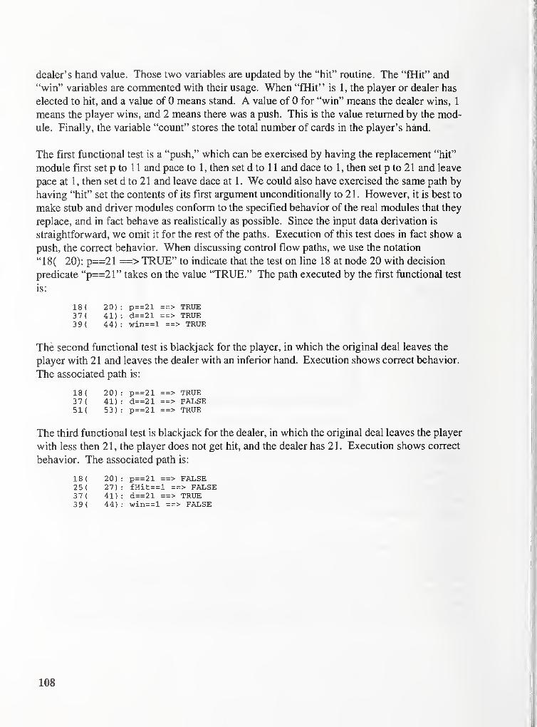
dealer's hand value. Those two variables are updated by the "hit" routine. The "fHit" and

"win" variables are commented with their usage. When "fHit" is 1, the player or dealer has

elected to hit, and a value of 0 means stand. A value of 0 for "win" means the dealer wins, 1

means the player wins, and 2 means there was a push. This is the value returned by the mod-

ule. Finally, the variable "count" stores the total number of cards in the player's hand.

The first functional test is a "push," which can be exercised by having the replacement "hit"

module first set p to 1 1 and pace to 1 , then set d to 11 and dace to 1 , then set p to 21 and leave

pace at 1, then set d to 21 and leave dace at 1. We could also have exercised the same path by

having "hit" set the contents of its first argument unconditionally to 2 1 . However, it is best to

make stub and driver modules conform to the specified behavior of the real modules that they

replace, and in fact behave as realistically as possible. Since the input data derivation is

straightforward, we omit it for the rest of the paths. Execution of this test does in fact show a

push, the correct behavior. When discussing control flow paths, we use the notation

"18( 20): p==21 ==> TRUE" to indicate that the test on line 18 at node 20 with decision

predicate "p==21" takes on the value "TRUE." The path executed by the first functional test

is:

18 ( 20) : p==21 ==> TRUE37 ( 41): d==21 ==> TRUE39 { 44): win==l ==> TRUE

The second functional test is blackjack for the player, in which the original deal leaves the

player with 21 and leaves the dealer with an inferior hand. Execution shows correct behavior.

The associated path is:

18 ( 20) : p==21 ==> TRUE37 ( 41): d==21 ==> FALSE51{ 53): p==21 ==> TRUE

The third functional test is blackjack for the dealer, in which the original deal leaves the player

with less then 21, the player does not get hit, and the dealer has 21 . Execution shows correct

behavior. The associated path is:

18 ( 20) : p==21 ==> FALSE25( 27) : fHit==l ==> FALSE37 ( 41) : d==21 = => TRUE39 ( 44) : win==l ==> FALSE

108

The fourth functional test is a five-card win, in which the player accumulates five cards with-

out going over 21 and the dealer was not dealt blackjack. Execution shows correct behavior.

The associated path is:

18 { 20) p==21 > FALSE25{ 27) fHit== 1 ==> TRUE29{ 33) p>21 = => FALSE25( 27) fHit== 1 ==> TRUE29 ( 33) p>21 = =

>

FALSE25( 27) fHit== 1 ==> TRUE29 ( 33) p>21 = =

>

FALSE25( 27) fHit== 1 ==> FALSE37 ( 41) d==21 > FALSE51( 53) p==21 > FALSE51( 54) count

>

= 5 ==> TRUE

The fifth functional test is a win for the player in which neither the player nor the dealer takes

a hit, and neither has blackjack. Execution shows correct behavior. The associated path is:

18 ( 20) p==21 => FALSE25( 27) fHit== 1 ==> FALSE37 ( 41) d==21 => FALSE51( 53) p==21 => FALSE51( 54) count> 5 ==> FALSE59 ( 63) d<=16 => FALSE69( 76) p>d == > TRUE

The sixth functional test is a win for the dealer in which neither the player nor the dealer takes

a hit, and neither has blackjack. Execution shows correct behavior. The associated path is:

18( 20) p==21 ==> FALSE25{ 27) fHit== 1 ==> FALSE37 { 41) d==21 ==> FALSE51{ 53) p==21 ==> FALSE51{ 54) count>=5 ==> FALSE59{ 63) d<=16 ==> FALSE69{ 76) p>d == > FALSE

The seventh functional test is a win for the dealer in which the player is busted. Execution

shows correct behavior. The associated path is:

18 ( 20): p==21 ==> FALSE25 ( 27): fHit==l ==> TRUE29 ( 33) : p>21 ==> TRUE

The eighth functional test is a win for the player in which the dealer is busted. Execution


18 ( 20): p==21 ==> FALSE25( 27): fHit==l ==> FALSE37 ( 41): d==21 ==> FALSE51( 53): p==21 ==> FALSE51 { 54): count>=5 ==> FALSE59 ( 63) : d<=16 ==> TRUE61 ( 66) : d>21 ==> TRUE

109

The ninth functional test is a win for the dealer in which the player is hit to reach 21 and the

dealer has blackjack. Execution shows correct behavior. The associated path is:

18 ( 20) p==21 => FALSE25( 27) fHit== 1 ==> TRUE29 ( 33) p>21 = > FALSE25( 27) fHit== 1 ==> FALSE37 ( 41) d= = 21 => TRUE39 ( 44) win==l ==> FALSE

This concludes our initial set of functional tests. No error has been detected yet, and each test

increased ac by 1, so ac is now 9. The coverage analysis tool reports that one branch has not

yet been executed, "61( 66): d>21 ==> FALSE." This corresponds to the dealer taking a hit

without being busted. Since branches are usually easier to test than paths, and testing a previ-

ously unexecuted branch must increase ac, we construct a new test for this branch immedi-

ately. The test makes the dealer win the hand by hitting once and then standing. Execution


18 ( 20) p==21 FALSE25 ( 27) fHit== 1 ==> FALSE37 ( 41) d==21 ==> FALSE51( 53) p==21 FALSE51( 54) count>=5 ==> FALSE59 ( 63) d<=16 ==> TRUE61 ( 66) d>21 = => FALSE59 ( 63) d<=16 ==> FALSE69( 76) p>d == > FALSE

All branches have now been covered. No error has been detected yet, and ac is now 10. The

coverage analysis tool reports that executing the following path would be sufficient to com-

plete basis path coverage:

18 ( 20) : p==21 FALSE25( 27) : fHit== 1 = FALSE37( 41) : d=:^21 FALSE51( 53) : p==21 TRUE

Unfortunately, this particular path is unrealizable, since the value of p is not altered between

the mutually exclusive "30( 13): p==21 ==> FALSE" and "62( 44): p==21 ==> TRUE"decision outcomes. If the basis completion path had been realizable, we could have just

derived the corresponding data, executed the test, and completed the testing process. For

modules as poorly structured as "hand," however, unrealizable paths are fairly common, so it

is important to be prepared for them. As discussed in section 9, the existence of unrealizable

paths does not necessarily mean that rc < v(G). To help determine whether a realizable alter-

native path can complete basis path testing, we use the dependency analysis technique. The

dependency analysis tool indicates that for every tested path, the total number of times

branches "39( 44): win== 1 ==> TRUE" and "5 1 ( 53): p==2 1 ==> TRUE" were executed is

equal to the number of times branch "18( 20): p==21 ==> TRUE" was executed. Note that

for any single path, none of those three decision outcomes can be executed more than once

and at most one of the first two can be executed. We may therefore rephrase the dependency

110

equation in terms of the module's functionality: The player has blackjack if and only if either

the result is a push or the player automatically wins with 21. Any test that does not satisfy this

dependency relationship will be independent of the current set of tests and increase ac, in this

case completing testing by making ac equal to v(G). On the other hand, if we can prove that

the dependency must hold for every feasible test, then we have shown that rc < v(G). Fortu-

nately, we can simplify the dependency even further, showing that rc = v(G) and giving a con-

cise characterization of all feasible basis completion paths. Note that if the player has

blackjack, the result must be either a push or an automatic win with 21 for the player. Also,

there is no way to reach a push result without the player having blackjack. Thus, a test breaks

the dependency relationship if and only if the player gets an automatic win with 21 without

having blackjack. This is clearly possible for the module as written, for example by having

the player reach exactly 21 after taking one hit. Execution of this test shows incorrect behav-

ior—the module declares an automatic win for the player without giving the dealer a chance

to take hits and win by also reaching 21. The specification states that the player can only win

"automatically" with either Blackjack or a five-card hand. As expected, this test completes

the basis set. The associated path is:

18( 20) : p==21 ==> FALSE25( 27) : fHit==l ==> TRUE29 ( 33) : p>21 ==> FALSE25( 27) : fHit:^=l ==> FALSE37( 41) : d==21 ==> FALSE51( 53) : p==21 ==> TRUE

Note that in addition to providing a test that detected the error, dependency analysis clarified

the nature of the error and gave a straightforward repair technique: replace the automatic win

test "51( 53): p==21" with "51( 53): win==l," since at that point win==l is precisely equiv-

alent to the player having blackjack. If the error is repaired in this manner, there will be no

way to break the dependency with a feasible path, and rc will therefore be reduced to 10.

Note also that structured testing is not guaranteed to detect the error, as can be seen from

dependency analysis. If the player reaches exactly 21 after taking at least three hits, the error

will not result in incorrect module output even though a dependency-breaking "incorrect"

control flow path is executed. The reason is that there is no difference in specified behavior

between an automatic win due to blackjack and an automatic win due to a five-card hand.

Hence, the five-card hand masks the error. This is the only situation in which structured test-

ing can fail to detect the error in the blackjack program, and as shown in section B-2 it is an

extremely rare situation during actual play of the game.

Ill

B.2 Experimental comparison ofstructured testing and branch

coverage

The "hand" module from section B-1 is one of several modules used in [WATSON4] to com-pare the error detection effectiveness of structured testing with branch coverage. The rest of

this appendix discusses that work. Although neither testing technique is guaranteed to detect

the error, structured testing performed dramatically better than branch coverage in the experi-

ment, which used random test data generation to simulate actual play.

B.2.1 Experimental design

The overall experimental design was to package the test module with a driver program that

accepts a random number seed as input, generates random test data from a realistic distribu-

tion, executes the test module with that data, analyzes the module's behavior, and returns an

exit code indicating whether an error was detected. A higher-level driver invokes the module

test driver with a sequence of seed values, uses an automated tool to measure the test coverage

level according to each criterion being compared, and tracks both the error detection and the

coverage results.

For both structured testing and branch coverage, 100 experimental trials were performed, in

each of which random test cases were generated iteratively until the current testing criterion

was satisfied. Four kinds of data were collected during each trial for the two testing criteria:

• Tests, the total number of tests executed until the criterion was satisfied

• Testsinc, the number of tests that increased coverage with respect to the criterion

• Detect, whether an error was detected during the trial

• Detectinc, whether an error was detected by a test that increased coverage

There is an important distinction between considering all tests and just considering the ones

that increased coverage. Considering all tests is essentially doing random testing while using

the coverage criterion as a stopping rule. This may be appropriate when detecting incorrect

program behavior is cheap, so that program behavior can be examined for each test. However,

the criteria comparison information from such an experiment tends to be diluted by the effec-

tiveness of the underlying random test data distribution. A criterion that requires more random

tests is likely to detect more errors, regardless of the value of the specific test cases that con-

tribute to satisfying the criterion. Therefore, we also consider just the tests that increase cover-

age. In that case, we factor out most of the influence of the underlying random test data

distribution by in effect considering random minimal test data sets that satisfy each criterion.

In addition to giving a more objective comparison, this more accurately models test effective-

ness when detecting incorrect program behavior is expensive, so that program behavior can

only be examined for tests that contribute to satisfaction of the test coverage criterion.

[WATS0N4]

112

B.2.2 Comparative frequency of error detection

Figure B-3 shows the data collected for the "hand" module during the experiment. Data about

number of tests is averaged over the 100 trials. Data about error detection is added for the 100

trials, giving a convenient interpretation as a percentage of trials in which errors were detected

by the criteria.

Structured Testing

Tests 45

Testsinc 1

1

Detect 97

Detectinc 96

Figure B-3. Experimental data.

B.2.3 Interpretation of experimental data

Structured testing decisively outperformed branch coverage at detecting the error while

requiring only 25% more total tests and 38% more tests that increase coverage. The most

notable feature of the data is the robustness of structured testing with respect to test set mini-

mization. Only 1% of the error detection effectiveness of structured testing was lost when

considering only tests that increased coverage, whereas the number of tests required was

reduced by 75%. For branch coverage, 38% of error detection effectiveness was lost, and the

number of tests required was reduced by 78%. This indicates that the effectiveness of struc-

tured testing is due to the criterion itself rather than just the number of tests required to satisfy

it. For the complete set of test programs used in [WATS0N4], structured testing preserved

94% of its error detection effectiveness when restricted to the 24% of test cases that increased

coverage.

Branch Coverage

36

8

85

53

113

ANNOUNCEMENT OF NEW PUBLICATIONS ONCOMPUTER SYSTEMS TECHNOLOGY

Superintendent of Documents

Government Printing Office

Washington, DC 20402

Dear Sir:

Please add my name to the announcement list of new publications to be issued in

the series: National Institute of Standards and Technology Special Publication 500-.

Name

Company

Address

City State Zip Code

(Notification key N-503)

Technical Publications

Periodical

Journal of Research of the National Institute of Standards and Technology—Reports NIST research

and development in those disciplines of the physical and engineering sciences in which the Institute is

active. These include physics, chemistry, engineering, mathematics, and computer sciences. Papers cover a

broad range of subjects, with major emphasis on measurement methodology and the basic technology

underlying standardization. Also included from time to time are survey articles on topics closely related to

the Institute's technical and scientific programs. Issued six times a year.

Nonperiodicals

Monographs—Major contributions to the technical literature on various subjects related to the

Institute's scientific and technical activities.

Handbooks—Recommended codes of engineering and industrial practice (including safety codes) devel-

oped in cooperation with interested industries, professional organizations, and regulatory bodies.

Special Publications—Include proceedings of conferences sponsored by NIST, NIST annual reports, and

other special publications appropriate to this grouping such as wall charts, pocket cards, and bibliographies.

National Standard Reference Data Series—Provides quantitative data on the physical and chemical

properties of materials, compiled from the world's literature and critically evaluated. Developed under a

worldwide program coordinated by NIST under the authority of the National Standard Data Act (Public

Law 90-396). NOTE: The Journal of Physical and Chemical Reference Data (JPCRD) is published

bimonthly for NIST by the American Chemical Society (ACS) and the American Institute of Physics (AIP).

Subscriptions, reprints, and supplements are available from ACS, 1155 Sixteenth St., NW, Washington, DC20056.

Building Science Series—Disseminates technical information developed at the Institute on building

materials, components, systems, and whole structures. The series presents research results, test methods, and

performance criteria related to the structural and environmental functions and the durability and safety

characteristics of building elements and systems.

Technical Notes—Studies or reports which are complete in themselves but restrictive in their treatment of

a subject. Analogous to monographs but not so comprehensive in scope or definitive in treatment of the

subject area. Often serve as a vehicle for final reports of work performed at NIST under the sponsorship of

other government agencies.

Voluntary Product Standards—Developed under procedures published by the Department of Commercein Part 10, Title 15, of the Code of Federal Regulations. The standards establish nationally recognized

requirements for products, and provide all concerned interests with a basis for common understanding of

the characteristics of the products. NIST administers this program in support of the efforts of private-sector

standardizing organizations.

Order the following NIST publications—FIPS and NISTlRs—from the National Technical Information

Service, Springfield, VA 22161.

Federal Information Processing Standards Publications (FIPS PUB)—Publications in this series

collectively constitute the Federal Information Processing Standards Register. The Register serves as the

official source of information in the Federal Government regarding standards issued by NIST pursuant to

the Federal Property and Administrative Services Act of 1949 as amended. Public Law 89-306 (79 Stat.

1127), and as implemented by Executive Order 11717 (38 FR 12315, dated May 11, 1973) and Part 6 of

Title 15 CFR (Code of Federal Regulations).

NIST Interagency Reports (NISTIR)—A special series of interim or final reports on work performed by

NIST for outside sponsors (bodi government and nongovernment). In general, initial distribution is handled

by the sponsor; public distribution is by the National Technical Information Service, Springfield, VA 22161,

in paper copy or microfiche form.

^ 2

1 1.< 3» ft

c

8

=r J o •

O (V 3 I—-1 o p Wg. 3- — re- => sr*©

o S2- "t

o 2.

c3 o sa

otoo00so

8

GO O

1.1- 3

re<inn