Introduction to Molecular Dynamics (MD) Simulations

Eduardo M. BringaCONICET/ Instituto de Ciencias Básicas, Universidad Nacional de Cuyo, Mendoza

(ebringa@yahoo.com)

First Argentinean School on GPUs for Scientific Applications Córdoba, May 2011Córdoba, May 2011

Collaborators:Emmanuel Millán, C. Ruestes, C. Garcia Garino

(UN Cuyo), A. Higginbotham (Oxford)

Outline• Introduction:a) Why do we need atomistic simulations?b) Where does molecular dynamics (MD) fit in the simulation map?•Atomistic Simulations:

a) What is MD?b) What can MD do for you? What can you do to make it faster?c) Caveats?d) Future perspective • Examples • MD code• Auxiliary code: Viz and data analysis.• Summary and conclusions

Mecánica

1 metro= 1,000,000,000 nanometros

1 metro= 1,000,000 micrones

¿ Qué es la nanotecnología?

Tight Binding

MD

del continuo

Espesor cabello humano ~ 200 µm

Estafilococo ~ 1 µm

Rinovirus ~ 200 nm

Kaxiras’ web

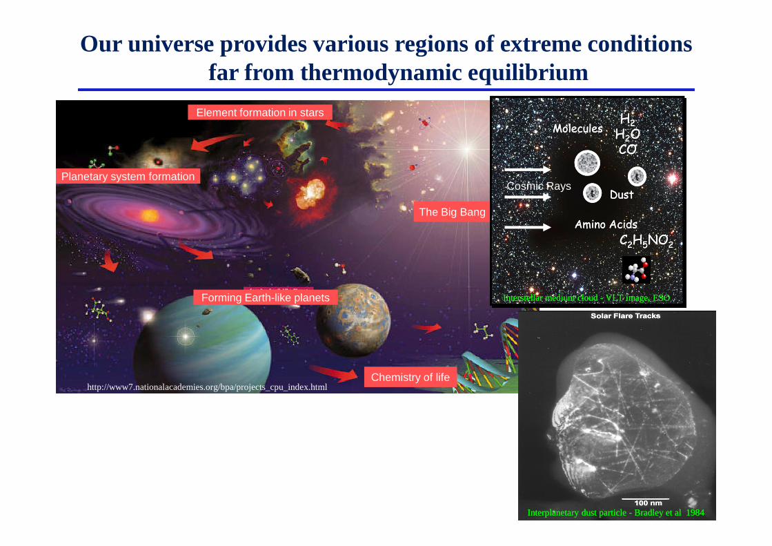
Our universe provides various regions of extreme conditions far from thermodynamic equilibrium

Element formation in stars

The Big Bang

Planetary system formation

tt

MoleculesMolecules

C2H

5NO

2C2H

5NO

2

H2

H2O

CO

H2

H2O

CO

Cosmic Raystt

DustDust

Amino AcidsAmino Acids

Forming Earth-like planets

Chemistry of lifehttp://www7.nationalacademies.org/bpa/projects_cpu_index.html

Interstellar medium cloud - VLT image, ESOInterstellar medium cloud - VLT image, ESO

Interplanetary dust particle - Bradley et al 1984Interplanetary dust particle - Bradley et al 1984

Nanocrystales (nc) tienen propiedades macro interesantes, incluyendo extrema dureza, debido a escala nano

Extensibilidad superplasticancCu (28 nm) Lu et al, Science (2000)

Mas fuerte y ~ elastoplasticidadperfectaChampion et al, Science (2003)

~100 nm grainsdε/dt=5 10-6/s

Ingrediente crucial en comportamiento de nc: la fraction de bordes de grano es (GB) muy alta

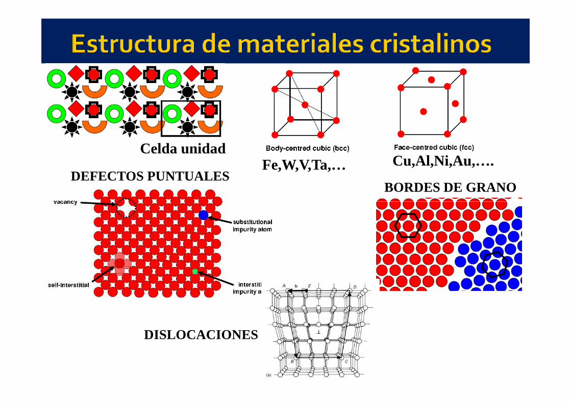
Celda unidad

DEFECTOS PUNTUALESBORDES DE GRANO

Cu,Al,Ni,Au,….Fe,W,V,Ta,…

DISLOCACIONES

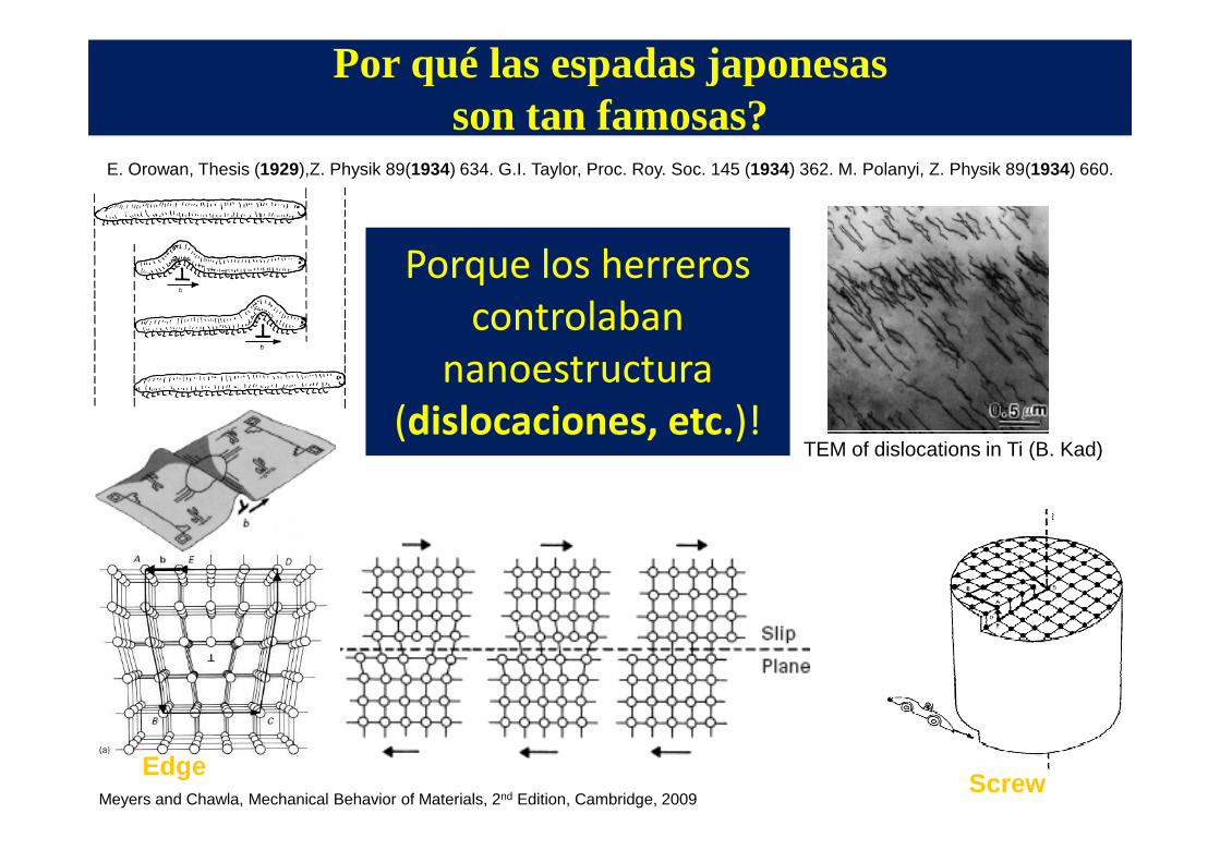
Por qué las espadas japonesas son tan famosas?

E. Orowan, Thesis (1929),Z. Physik 89(1934) 634. G.I. Taylor, Proc. Roy. Soc. 145 (1934) 362. M. Polanyi, Z. Physik 89(1934) 660.

Porque los herreros

controlaban

nanoestructura

(dislocaciones, etc.)!

Meyers and Chawla, Mechanical Behavior of Materials, 2nd Edition, Cambridge, 2009

EdgeScrew

TEM of dislocations in Ti (B. Kad)(dislocaciones, etc.)!

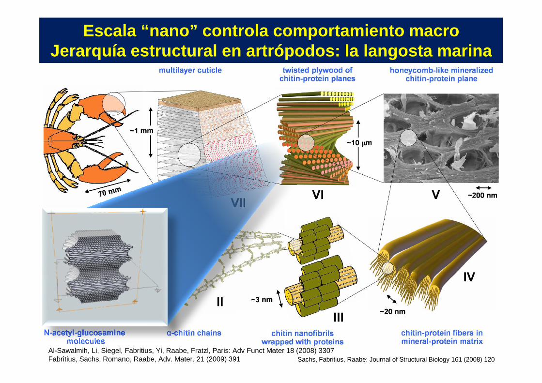
Escala “nano” controla comportamiento macroJerarquía estructural en artrópodos: la langosta ma rina

8Al-Sawalmih, Li, Siegel, Fabritius, Yi, Raabe, Fratzl, Paris: Adv Funct Mater 18 (2008) 3307Fabritius, Sachs, Romano, Raabe, Adv. Mater. 21 (2009) 391 Sachs, Fabritius, Raabe: Journal of Structural Biology 161 (2008) 120

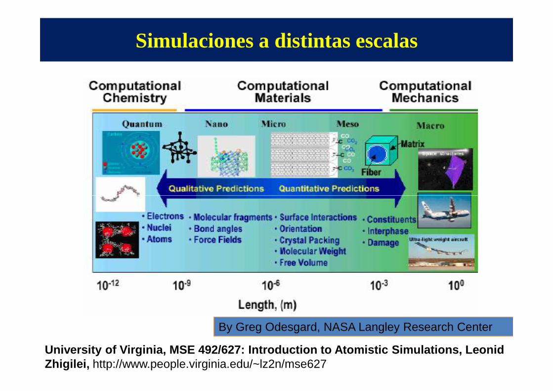
Simulaciones a distintas escalas

By Greg Odesgard, NASA Langley Research Center

University of Virginia, MSE 492/627: Introduction t o Atomistic Simulations, Leonid Zhigilei, http://www.people.virginia.edu/~lz2n/mse627

Herramientas de simulación

Dzwinel W, Alda W, Kitowski J, Yuen DA, Molecular Simulation, 20/6, 361-384 (2000)

Nuevas técnicas experimentales están alcanzando escalas de tiempo y longitud comparables con las de simulaciones atomísticas

Control de procesos bajo condiciones extremas ����

producción de nuevos materiales y comprensión de procesos astrofísicos

Una herramienta muy útil para estudiar materiales:Dinámica Molecular clásica =Molecular Dynamics=MD

• N partículas clásicas. Partícula i con posición r i, tiene velocidad vi

y aceleración ai.

• Partículas interactúan a través de un potencial empírico, V(r1,.., r i,.., rN), que generalmente incluye interacciones de muchos cuerpos.

i

j

k

Fji

Fjk

Fij

FkjFki

Fik

• Partículas obedecen las ecuaciones de movimiento de Newton. Partícula i, masa mi: F i = -∇iV(r1,.., r i,.., rN)= mi ai = mi (d2r i /dt2)

• Volumen<0.5 µm3~109 átomos)

• Tiempos t<1 ns, ∆t~1 fs)

• Varios integradores disponibles

• Pueden incorporarse efectoselectrónicos (Koci et al, PRB 2006).

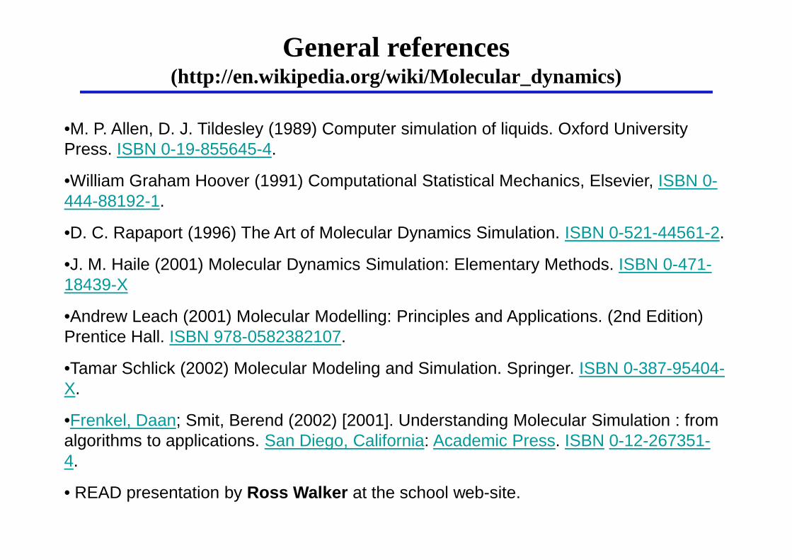
•M. P. Allen, D. J. Tildesley (1989) Computer simulation of liquids. Oxford University Press. ISBN 0-19-855645-4.

•William Graham Hoover (1991) Computational Statistical Mechanics, Elsevier, ISBN 0-444-88192-1.

•D. C. Rapaport (1996) The Art of Molecular Dynamics Simulation. ISBN 0-521-44561-2.

•J. M. Haile (2001) Molecular Dynamics Simulation: Elementary Methods. ISBN 0-471-18439-X

General references (http://en.wikipedia.org/wiki/Molecular_dynamics)

18439-X

•Andrew Leach (2001) Molecular Modelling: Principles and Applications. (2nd Edition) Prentice Hall. ISBN 978-0582382107.

•Tamar Schlick (2002) Molecular Modeling and Simulation. Springer. ISBN 0-387-95404-X.

•Frenkel, Daan; Smit, Berend (2002) [2001]. Understanding Molecular Simulation : from algorithms to applications. San Diego, California: Academic Press. ISBN 0-12-267351-4.

• READ presentation by Ross Walker at the school web-site.

Compile mdtot.c with desired options to obtain executable

Execute (interactive/not interactive)

Setup-1:Initialize arrays. Convert different units to MD units. Open input/output files.Iterations = 0

Input file:Total number of iterations=Max-iteraTotal time/iteration=time-End

iterations<=Max-itera

Calculate new r,v,a. Apply Boundary conditions.Calculate total energy, temperature,

Typical MD code flow chart

Final-2:calculate different quantities: sputtering yield for this particular run, save final configuration if needed, etc.

iterations+1Setup-2: Initial positions velocities of atoms, etc. Time=0

Final-1:Average different calculated quantities, like sputtering yield, etc. Save important data. Close files.

YESNO

MD-Step:Calculate DeltaTTime=time+DeltaT

iterations<=Max-itera

Time<time-End

EXIT

Calculate total energy, temperature, etcetera Excite the sample.Every timeAvg calculate certain parameters and save them in corresponding files, like temperature profiles and order parameterDraw snapshots if needed

NOYES

Post-run Analysis programs

Alejandro Strachan, http://nanohub.org/resources/5838#series

Alejandro Strachan, http://nanohub.org/resources/5838#series

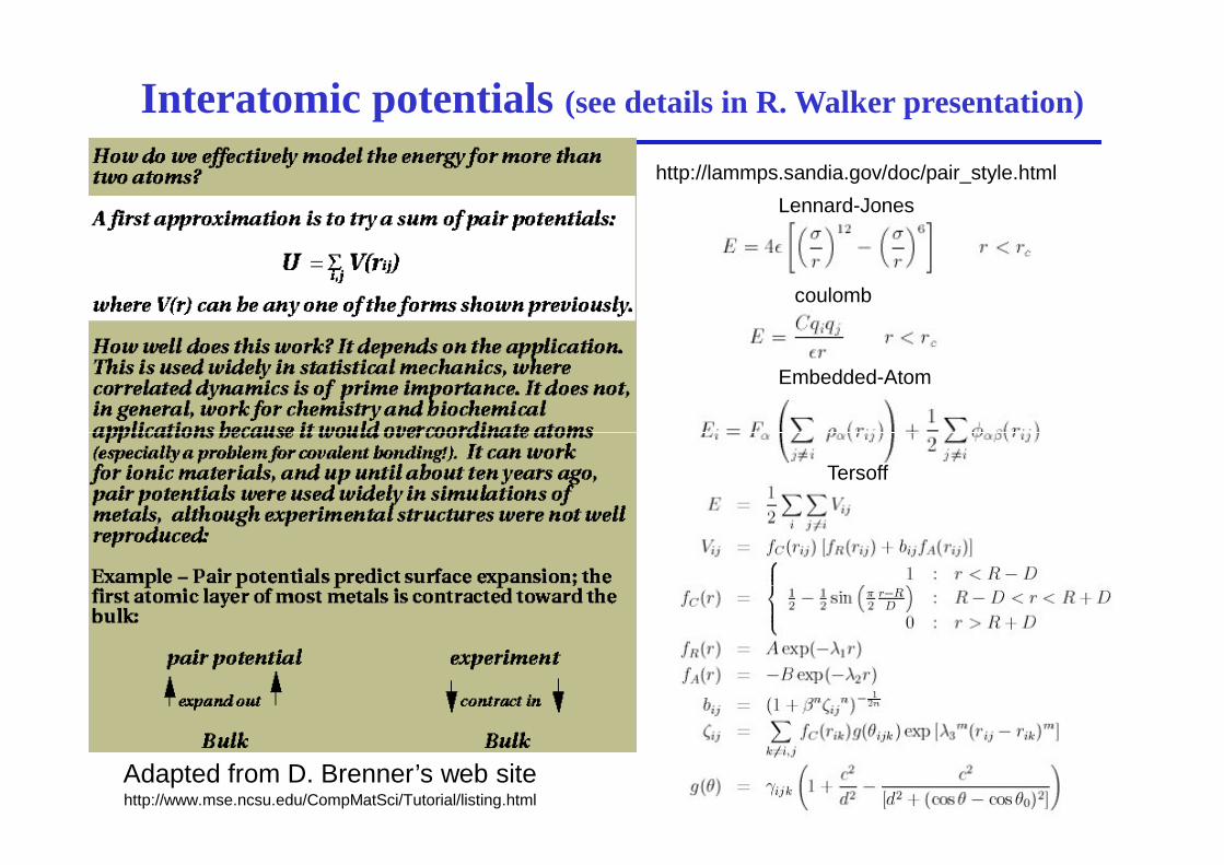
Interatomic potentials (see details in R. Walker presentation)

Lennard-Jones

coulomb

Embedded-Atom

http://lammps.sandia.gov/doc/pair_style.html

Adapted from D. Brenner’s web sitehttp://www.mse.ncsu.edu/CompMatSci/Tutorial/listing.html

Tersoff

Interatomic potentials

Many-body pots are a way to improve on

two-body interactions

Adapted from D. Brenner’s web sitehttp://www.mse.ncsu.edu/CompMatSci/Tutorial/listing.html

With MD you can obtain….

“Real” time evolution of your system.

Thermodynamic properties, including T(r,t) temperature profiles that can be used in

•Can simulate only small samples (L<1 µm, up to ~109 atoms).•Can simulate only short times (t<1 µs, because ∆t~1 fs).•Computationally expensive (weeks)

Limitations of MD

Atomistic simulations are extremely helpful but … still have multiple limitations

profiles that can be used in rate equations.

Mechanical properties, including elastic and plastic behavior.

Surface/bulk/cluster growth and modification.

X-ray and “IR” spectra

Etcetera …

(weeks)•Interaction potentials for alloys, molecular solids, and excited species not well know.•Despite its limitationsMD is a very powerful tool to study nanosystems.

How much does classical MD cost? (very rough estimate for short range potentials)Nsteps =number of time steps; N=total number of atoms. Rcut=potential cut-off; N cut=number of atoms within R cut . Can influence timing. F=cost of evaluating forces for a given atom potential dependent: if F LJ=1 ���� FEAM~3, FAIREBO~50, FREAXFF~300

COST ∝∝∝∝ F Nsteps f(N) ∝∝∝∝ F Nsteps f(N)

Serial codes:No neighbor list � f(N) ∝∝∝∝ N2 (Only practical for N<2,000 -5,000)No neighbor list � f(N) ∝∝∝∝ N (Only practical for N<2,000 -5,000)

Neighbor list ���� f(N) ∝∝∝∝ Npair potential ���� memory limited: neighbor list 1 GB RAM for N~500,00 0 many-body potentials ���� F very costly ���� practical for N<5,000-30,000 atoms

N large and/or F costly ���� need parallel code

Parallel Codes:Domain decomposition ���� f(N) ∝∝∝∝ NPRICE: communication overhead ���� impractical if N/CPU < 2,000-5,000 MDCASK (LLNL): evaluation of F~80%, communication~15%, various~5%.

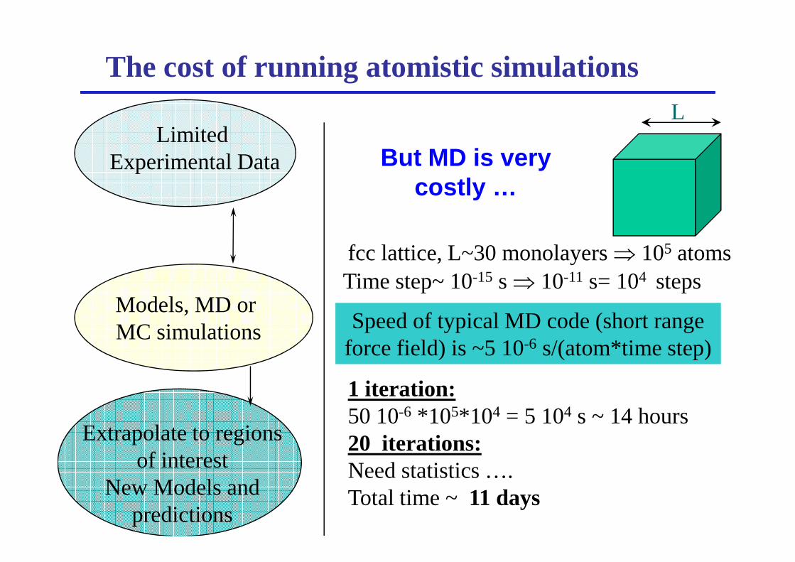
The cost of running atomistic simulationsL

fcc lattice, L~30 monolayers ⇒ 105 atoms Time step~ 10-15 s ⇒ 10-11 s= 104 steps

But MD is very costly …

Limited Experimental Data

Speed of typical MD code (short range force field) is ~5 10-6 s/(atom*time step)

Time step~ 10-15 s ⇒ 10-11 s= 104 steps

1 iteration: 50 10-6 *105*104 = 5 104 s ~ 14 hours20 iterations:Need statistics ….Total time ~ 11 days

Models, MD or MC simulations

Extrapolate to regions of interest

New Models and predictions

Algunas aéreas de simulación donde se necesitan urgentes contribuciones matemáticas

• Técnicas multi-escala temporales: dinámica ficticia, “rare events”, etc.

• Técnicas multi-escala espaciales: problemas de frontera y acoplamiento entre escalas, incluyendo problemas “estáticos” y dinámicos.

• Inestabilidades y fragmentación: RT, RM, Euler, parámetros de orden, etc.

• Medios desordenados: estructura, plasticidad y viscosidad en vidrios y medios porosos.

• Propagación de ondas en medios no homogéneos, con propiedades no-lineales y posibles cambios de fase.lineales y posibles cambios de fase.

• Métodos de minimización (energía, funciones potencial, intercambio de carga, etc.) y para hallar “caminos de reacción”

• Data mining en archivos de TBs: como encontrar la aguja en el pajar.

• Como graficar en paralelo y con interfaces “amigables”.

• Nuevos algoritmos eficientes en paralelos para problemas mucho mas complejos que los que se resuelven muy bien en sistemas pequeños en serie: Monte Carlo, métodos de minimización, interacciones de largo alcance, FFT, códigos CFD, etc.

Algún voluntario?

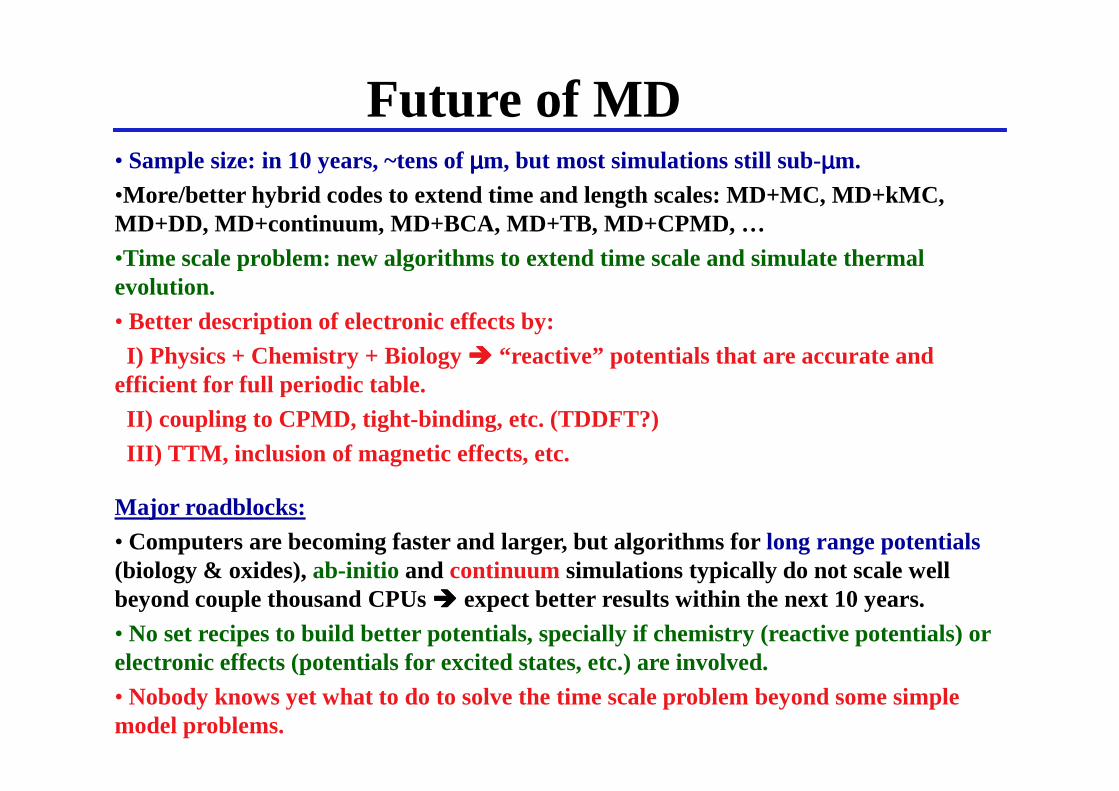
Future of MD• Sample size: in 10 years, ~tens of µµµµm, but most simulations still sub-µµµµm. •More/better hybrid codes to extend time and length scales: MD+MC, MD+kMC, MD+DD, MD+continuum, MD+BCA, MD+TB, MD+CPMD, …•Time scale problem: new algorithms to extend time scale and simulate thermal evolution.• Better description of electronic effects by: I) Physics + Chemistry + Biology ���� “reactive” potentials that are accurate and

efficient for full periodic table.efficient for full periodic table.II) coupling to CPMD, tight-binding, etc. (TDDFT?)III) TTM, inclusion of magnetic effects, etc.

Major roadblocks:• Computers are becoming faster and larger, but algorithms for long range potentials(biology & oxides), ab-initio and continuum simulations typically do not scale well beyond couple thousand CPUs ���� expect better results within the next 10 years.• No set recipes to build better potentials, specially if chemistry (reactive potentials) or electronic effects (potentials for excited states, etc.) are involved.• Nobody knows yet what to do to solve the time scale problem beyond some simple model problems.

Coupling TIME and length scales ….

• Choose set of parameters from MD, save those parameters and “pass” them to a “higher” level code. Example: calculate defect concentrations as the initial configuration for a kinetic Monte Carlo code.

• Use some accelerated technique, which boost the time • Use some accelerated technique, which boost the time step, for instance “TAD” by A. Voter (LANL). Very expensive computationally, practical only for “2D” simulations or small 3D simulations.

• Several people are currently working on improving this situation … Keep tuned!

Definition of temperature in nano systems

Jellinek & Goldberg, Chem Phys. (2000)

Pearson et al, PRB (1985)

Usual: (3/2) N kB T = Ekin

Nano Systems:

Correction due to non-zero flow velocity <v>: Correction due to non-zero flow velocity <v>:

Ekin� (m/2) (v - <v>)2

Ekin>0, but T=0

v

“Partial” T’s: T rot, Tvib, Tij

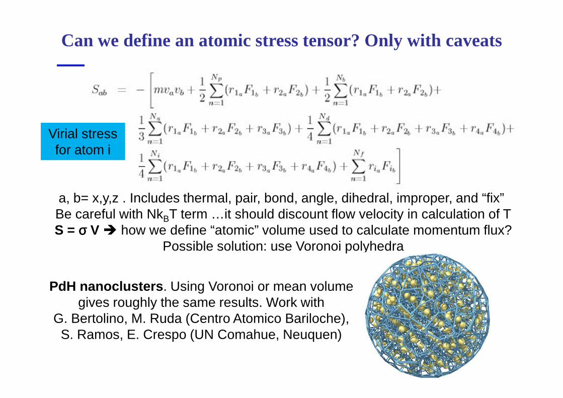
Can we define an atomic stress tensor? Only with caveats

a, b= x,y,z . Includes thermal, pair, bond, angle, dihedral, improper, and “fix”

Virial stress for atom i

PdH nanoclusters . Using Voronoi or mean volume gives roughly the same results. Work with

G. Bertolino, M. Ruda (Centro Atomico Bariloche), S. Ramos, E. Crespo (UN Comahue, Neuquen)

a, b= x,y,z . Includes thermal, pair, bond, angle, dihedral, improper, and “fix” Be careful with NkBT term …it should discount flow velocity in calculation of TS = σσσσ V � how we define “atomic” volume used to calculate momentum flux?

Possible solution: use Voronoi polyhedra

4

6

8

diam

etro

(nm

)

Diamante

Grafito

Diagrama de fase de nanoclusters de carbono

Diagrama para una muestra infinita Diagrama para una muestra esférica

Pext =0 GPa

Pre

sión

(G

Pa)

(1700 MPa, 0 K) (12000 MPa, 5000 K)

P = 1700 + 2.06T

P= 4 γ /dEc. Laplace-Young :

d = 4 γ /(1700 + 2.06T )

en equilibrio

γ= (γD + γG )/2

0 500 1000 1500 2000 2500

2

Temperatura (K)

Diamante

Las transiciones diamante �grafito y grafito � diamante tienen cinéticas diferentes

Zhao, D. et al, “Size and temperature dependence of nanodiamond-nanographite transition related with

surface stress”, Diamond and Related Materials 11 (2002) 234.

Temperatura (K)

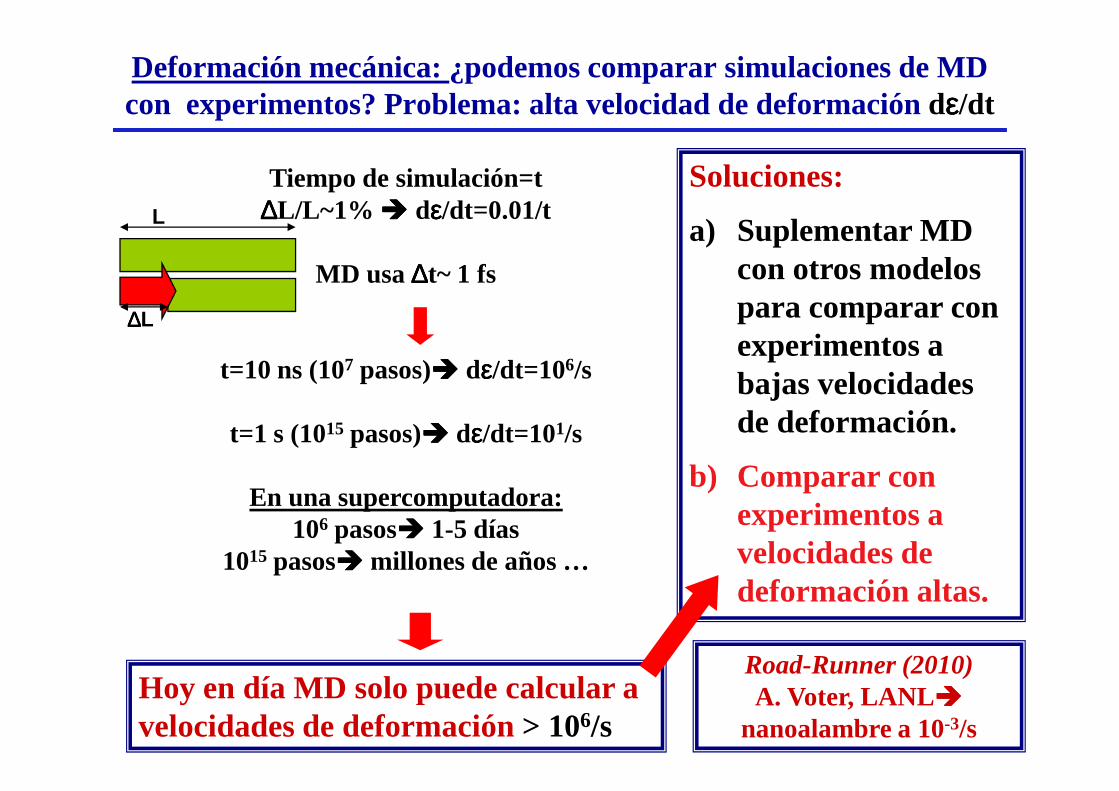
Deformación mecánica: ¿podemos comparar simulaciones de MD con experimentos? Problema: alta velocidad de deformación dεεεε/dt

Tiempo de simulación=t ∆∆∆∆L/L~1% ���� dεεεε/dt=0.01/t

MD usa ∆∆∆∆t~ 1 fs

t=10 ns (107 pasos)���� dεεεε/dt=106/s

Soluciones:

a) Suplementar MD con otros modelos para comparar con experimentos a bajas velocidades

∆∆∆∆L

L

Hoy en día MD solo puede calcular a velocidades de deformación > 106/s

t=1 s (1015 pasos)���� dεεεε/dt=101/s

En una supercomputadora:106 pasos���� 1-5 días

1015 pasos���� millones de años …

bajas velocidades de deformación.

b) Comparar con experimentos a velocidades de deformación altas.

Road-Runner (2010)A. Voter, LANL ����

nanoalambre a 10-3/s

Las velocidades de deformación altas son de interés general

¿Como se deforman/rompen los materiales cuando los empujo/tiro muy rápido?

Los láseres de alta potencia producen ondas de choque ����

empujan materiales con velocidades de deformación de 106/s-109/s

• Necesitamos entender el comportamiento de materiales bajo condiciones extremas. Regiones sin explorar ����ciencia de los materiales novedosa

• Podemos crear materiales mejores y novedosos? Si

•Velocidad de deformación láseres ~ MD

•Presión ~ 106 x presión atmosférica

•Escalas de tiempo y longitud sobrepuestas con MD

empujan materiales con velocidades de deformación de 10/s-10 /s

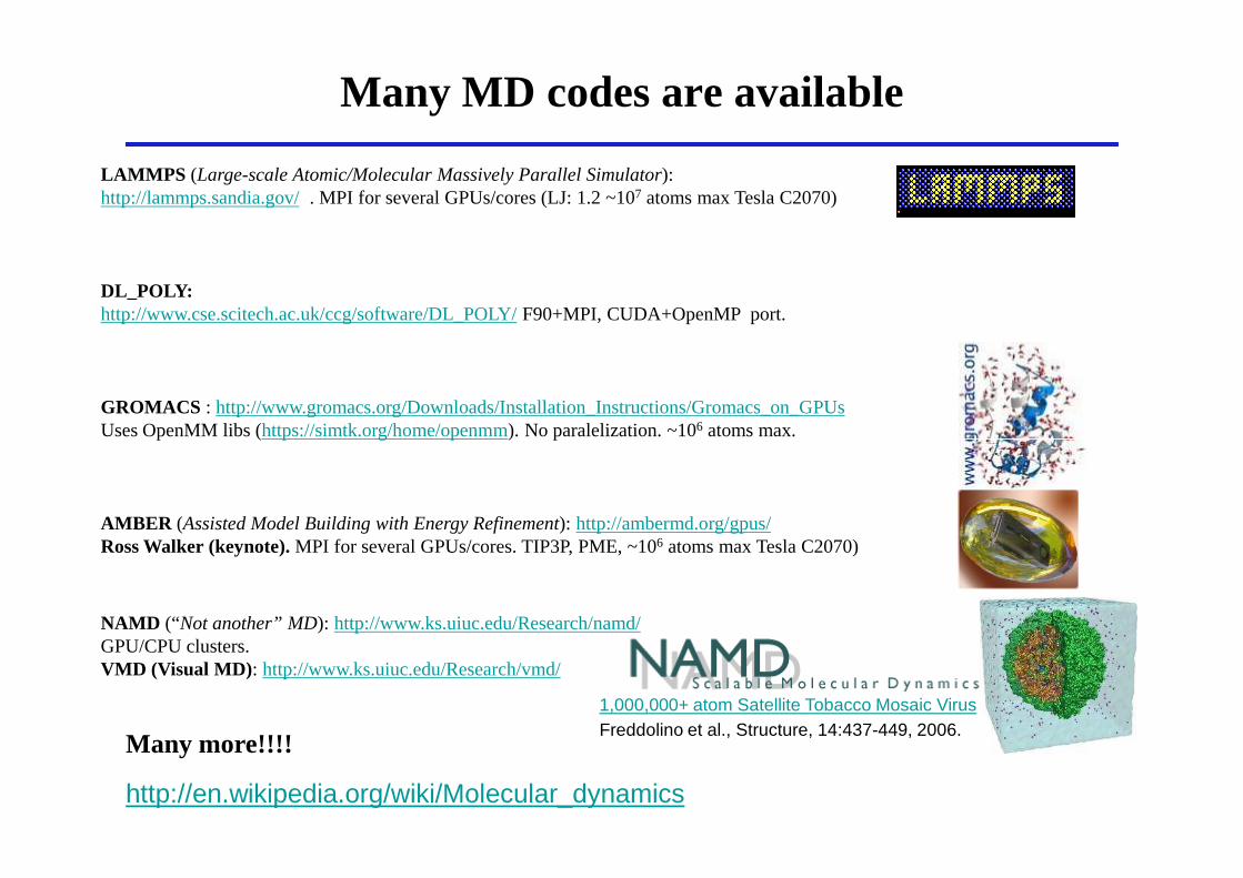
Many MD codes are available

LAMMPS (Large-scale Atomic/Molecular Massively Parallel Simulator): http://lammps.sandia.gov/. MPI for several GPUs/cores (LJ: 1.2 ~107 atoms max Tesla C2070)

DL_POLY:http://www.cse.scitech.ac.uk/ccg/software/DL_POLY/F90+MPI, CUDA+OpenMP port.

GROMACS : http://www.gromacs.org/Downloads/Installation_Instructions/Gromacs_on_GPUsUses OpenMM libs (https://simtk.org/home/openmm). No paralelization. ~106 atoms max.

AMBER (Assisted Model Building with Energy Refinement): http://ambermd.org/gpus/Ross Walker (keynote).MPI for several GPUs/cores. TIP3P, PME, ~106 atoms max Tesla C2070)

Uses OpenMM libs (https://simtk.org/home/openmm). No paralelization. ~10atoms max.

NAMD (“Not another” MD): http://www.ks.uiuc.edu/Research/namd/GPU/CPU clusters. VMD (Visual MD) : http://www.ks.uiuc.edu/Research/vmd/

1,000,000+ atom Satellite Tobacco Mosaic VirusFreddolino et al., Structure, 14:437-449, 2006.

Many more!!!!

http://en.wikipedia.org/wiki/Molecular_dynamics

LAMMPS ( http://lammps.sandia.gov/)

Some of my personal reasons to use LAMMPS:

1) Free, open source (GNU license).

2) Easy to learn and use:

(a) extensive docs :http://lammps.sandia.gov/doc/Section_commands.html#3_5(b) mailing list in sourceforge.

(c) responsive developers and user community.

3) It runs efficiently in my laptop (2 cores) and in BlueGeneL (100 K cores), including parallel I/O, with the same input script.

4) Very efficient parallel energy minimization, including cg & FIRE.

5) Includes many-body, bond order, & reactive potentials. Can simulate inorganic & bio systems, granular and CG systems.

6) Can do extras like DSMC, TAD, NEB, TTM, semi-classical methods, etc.

7) Extensive set of analysis routines: coordination, centro, cna, etc.

8) Easy to write analysis inside input, using something similar to pseudo-code.

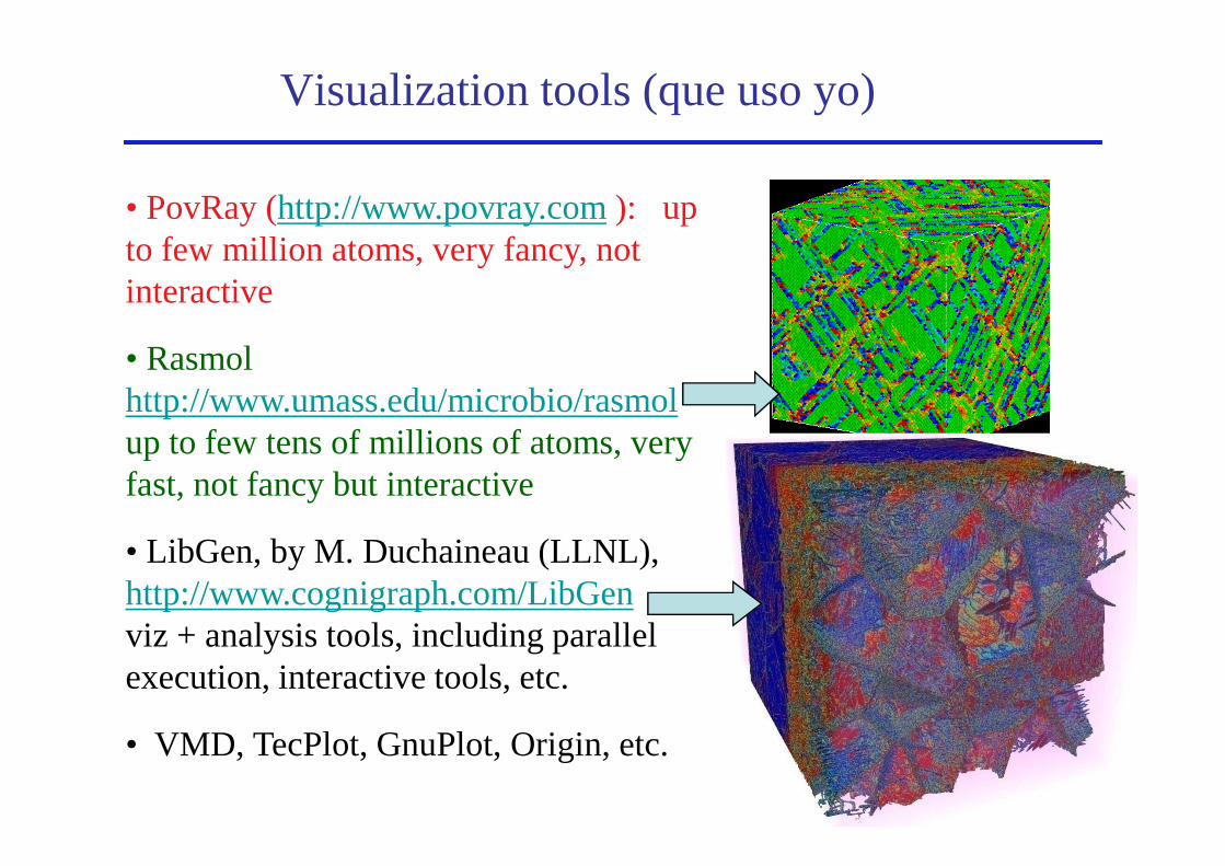
Visualization tools (que uso yo)

• PovRay (http://www.povray.com): up to few million atoms, very fancy, not interactive

• Rasmol http://www.umass.edu/microbio/rasmolup to few tens of millions of atoms, very up to few tens of millions of atoms, very fast, not fancy but interactive

• LibGen, by M. Duchaineau (LLNL), http://www.cognigraph.com/LibGenviz + analysis tools, including parallel execution, interactive tools, etc.

• VMD, TecPlot, GnuPlot, Origin, etc.

Resumen y perspectivas futuras

• Termodinámica y mecánica estadística equilibrio muy “robusta”, incluyendo situaciones con pocos átomos y no estacionarias.

• Nuevos diagnósticos ultra-rápidos permitirán explorar nuevas regiones del espacio de las fases, con simulaciones a espacio de las fases, con simulaciones a escala similar.

• Nuevas computadoras, junto a nuevos programas y modelos, permitirán una comparación directa entre simulaciones atomísticas y experimentos. Utilización de GPUs en cálculos de clusters o sistemas relativamente pequeños.