ee123 digital signal processingee123/sp18/notes/lecture...digital signal processing lecture 10a...

M. Lustig, EECS UC Berkeley

EE123Digital Signal Processing

Lecture 10AFilter Design


Linear Filter Design

• Used to be an art– Now, lots of tools to design optimal filters

• For DSP there are two common classes– Infinite impulse response IIR– Finite impulse response FIR

• Both classes use finite order of parameters for design

• We will cover FIR designs, briefly mention IIR


What is a linear filter

• Attenuates certain frequencies• Passes certain frequencies• Affects both phase and magnitude • IIR

– Mostly non-linear phase response– Could be linear over a range of frequencies

• FIR– Much easier to control the phase– Both non-linear and linear phase


FIR Design by Windowing

• Given desired frequency response, Hd(ejω) , find an impulse response

• Obtain the Mth order causal FIR filter by truncating/windowing it

hd[n] =1

2⇡

Z ⇡

�⇡Hd(e

j!)ej!nd!

ideal

h[n] =

⇢hd[n]w[n] 0 n M0 otherwise

�

|H(ej!)|



• We already saw that,

• For Boxcar (rectangular) window

H(ej!) = Hd(ej!) ⇤W (ej!)

W (ej!) = e�j!M2sin(w(M + 1)/2)

sin(w/2)

\W (ej!)

* =|W (ej!)|Hd(e

j!)

periodic conv.



|H(ej!)|

ωcωc

transition width

stop-band ripple

pass-band ripple

ideal


Windows (as defined in MATLAB)

-5 0 50

0.2

0.4

0.6

0.8

1

n

w[n

]

hann(M+1), M = 8

-5 0 50

0.2

0.4

0.6

0.8

1

n

w[n

]

hann(M+1), M = 8

-5 0 50

0.2

0.4

0.6

0.8

1

n

w[n

]

hanning(M+1), M = 8

-5 0 50

0.2

0.4

0.6

0.8

1

n

w[n

]

hanning(M+1), M = 8

-5 0 50

0.2

0.4

0.6

0.8

1

n

w[n

]

hamming(M+1), M = 8

-5 0 50

0.2

0.4

0.6

0.8

1

n

w[n

]

hamming(M+1), M = 8

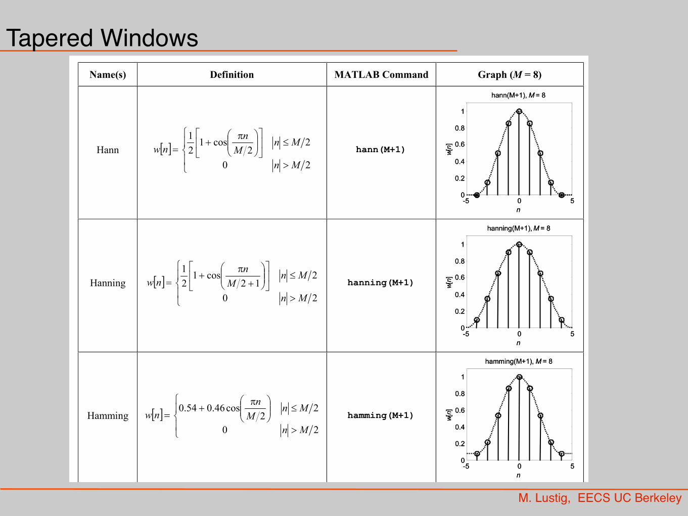
Name(s) Definition MATLAB Command Graph (M = 8)

Hann > @ nw°¯

°®

!

d»¼

º«¬

ª¸̧¹

·¨̈©

§ S�

20

22

cos12

1

Mn

MnM

n

hann(M+1)

Hanning > @ nw°¯

°®

!

d»¼

º«¬

ª¸̧¹

·¨̈©

§�

S�

20

212

cos12

1

Mn

MnM

n

hanning(M+1)

Hamming > @ nw°¯

°®

!

d¸̧¹

·¨̈©

§ S�

20

22

cos46.054.0

Mn

MnM

n

hamming(M+1)

Miki Lustig UCB. Based on Course Notes by J.M Kahn Spring 2014, EE123 Digital Signal Processing

Tapered Windows


Window Example

0 0.5 1 1.5 2 2.5 3

-0.2

0

0.2

0.4

0.6

0.8

1

:

W(ej :

)M = 16

Boxcar

Triangular

0 0.5 1 1.5 2 2.5 3

-0.2

0

0.2

0.4

0.6

0.8

1

:

W(ej :

)

M = 16

Hanning

Hamming

0 0.5 1 1.5 2 2.5 3-70

-60

-50

-40

-30

-20

-10

0

:

20

lo

g1

0|W

(ej :

)|

M = 16

Boxcar

Triangular

0 0.5 1 1.5 2 2.5 3-70

-60

-50

-40

-30

-20

-10

0

:

20

lo

g1

0|W

(ej :

)|

M = 16

Hanning

Hamming

Miki Lustig UCB. Based on Course Notes by J.M Kahn Spring 2014, EE123 Digital Signal Processing

ωω

ω ω

Tradeoff - Ripple vs Transition Width

Python: scipy.filter.firwin


FIR Filter Design

• Choose a desired frequency response Hd(ejω) – non causal (zero-delay), and infinite imp. response– If derived from C.T, choose T and use:

• Window:– Length M+1 ⇔ affects transition width

– Type of window ⇔ transition-width/ ripple

– Modulate to shift impulse response

Hd(ej!) = Hc(j

⌦

T)

Hd(ej!)e�j!M

2

• Determine truncated impulse response h1[n]

• Apply window

• Check:– Compute Hw(ejω), if does not meet specs increase M or change window


FIR Filter Design

h1[n] =

⇢12⇡

R ⇡�⇡ Hd(ej!)e�j!M

2 ej!n 0 n M

0 otherwise

hw[n] = w[n]h1[n]

h1[n] =

(sin(!c(n�M/2))

⇡(n�M/2) 0 n M

0 otherwise


Example: FIR Low-Pass Filter Design

Hd(ej!) =

⇢1 |!| !c

0 otherwise

Choose M ⇒ Window length and set

H1(ej!) = Hd(e

j!)e�j!M2

!c

⇡sinc(

!c

⇡(n�M/2))


Example: FIR Low-Pass Filter Design

• The result is a windowed sinc function

• High Pass Design:– Design low pass hw[n]– Transform to hw[n](-1)n

• General bandpass–Transform to 2hw[n]cos(ω0n)

hw[n] = w[n]h1[n]

!c

⇡sinc(

!c

⇡(n�M/2))


Characterization of Filter Shape

Time-Bandwidth Product, a unitless measure T(BW) = (M+1)ω/2π ⇒ also, total # of zero crossings

TBW=2 TBW=4 TBW=8 TBW=12

Larger TBW ⇒ More of the “sinc” functionhence, frequency response looks more like a rect function


TBW = 2, M=16

TBW = 8, M=16

TBW = 16, M =32


Frequency Response Profile

TBW=2 TBW=12

π-π π/12-π/12 π/2-π/2

Q: What are the lengths of these filters in samples?

2 = (M+1)*(π/6) / (2π) ⇒ M=23 12= (M+1)*(π) / (2π) ⇒ M=23

Note that transition is the same!

• To design order M filter:• Over-Sample/discretize the frequency response

at P points where P >> M (P=15M is good)

– Sampled at:– Compute h1[n] = IDFTP(H1[k])– Apply M+1 length window:


Alternative Design Through FFT

!k = k2⇡

P|k = [0, · · · , P � 1]

H1(ej!k) = Hd(e

j!k)e�j!kM2

hw[n] = w[n]h1[n]


Example: signal.firwin2

• signal.firwin2(M+1,omega_vec/pi, amp_vec)• taps1 = signal.firwin2(30, [0.0,0.2,0.21,0.5,

0.6, 1.0], [1.0, 1.0, 0.0,0.0,1.0,0.0])impulse response

magnitude frequency response


Optimal Filter Design

• Window method–Design Filters heuristically using windowed sinc functions

• Optimal design– Design a filter h[n] with H(ejω)– Approximate Hd(ejω) with some optimality criteria - or satisfies specs.

!p !s ⇡

Hd(ej!)

minimize

Z

!2care|H(ej!)�Hd(e

j!)|2d!

minimize

Z ⇡

�⇡W (!)|H(ej!)�Hd(e

j!)|2d!


Optimality

• Least Squares:

Don’t Care

Variation: weighted least-squares


Optimality

• Chebychev Design (min-max)

– Parks-McClellan algorithm - equi-ripple– Also known as Remez exchange algorithms(signal.remez)

minimize!2care max |H(ej!)�Hd(ej!)|


Example of Complex FilterLarson et. al, “Multiband Excitation Pulses for Hyperpolarized 13C Dynamic Chemical Shift Imaging” JMR 2008;194(1):121-127

Hz

Need to design 11 taps filter with following frequency response:

-500 500

1

0

Don’t Care

Don’t CareD.C. D.C.

D.C.

ee123 digital signal processingee123/sp18/notes/lecture...digital signal processing lecture 10a...

Documents