efï¬cient management of multi-linked negotiation based on
TRANSCRIPT

Efficient Management of Multi-Linked Negotiation Based on a Formalized Model
Xiaoqin Zhang
Department of Computer and Information Science
University of Massachusetts at Dartmouth
Victor Lesser, Sherief Abdallah
Department of Computer Science
University of Massachusetts at Amherst
lesser, [email protected]
April 30, 2004
Abstract
A Multi-linked negotiation problem occurs when an agent needs to negotiate with multiple other agents about different subjects (tasks,
conflicts, or resource requirements), and the negotiation over one subject has influence on negotiations over other subjects. The solution
of the multi-linked negotiations problem will become increasingly important for the next generation of advanced multi-agent systems.
However, most current negotiation research looks only at a single negotiation and thus does not present techniques to manage and reason
about multi-linked negotiations. In this paper, we first present a technique based on the use of a partial-order schedule and a measure of
the schedule, called flexibility, which enables an agent to reason explicitly about the interactions among multiple negotiations. Next, we
introduce a formalized model of the multi-linked negotiation problem. Basedon this model, a heuristic search algorithm is developed
for finding a near-optimal ordering of negotiation issues and their parameters. Using this algorithm, an agent can evaluate and compare
different negotiation approaches and choose the best one. We show how an agent uses this technology to effectively manage interacting
negotiation issues. Experimental work is presented which shows the efficiency of this approach.
keywords: multiple related negotiations, agent reasoning and control, conflict resolution, performance optimization
1 Introduction
Multi-linked negotiation describes a situation where one agent needs to negotiate with multiple agents about different issues (tasks,
conflicts, or resource requirements), and the negotiation over one issue affects the negotiations over other issues. Ina multi-task,
resource-sharing environment, an agent needs to deal with multiple, related negotiation issues including: tasks contracted to other
agents, tasks requested by other agents, external resourcerequirements for local activities, and interrelationships among activities
distributed among different agents.
Consider the following example shown in Figure 1, which is a simplified supply chain containing four agents. TheConsumer
Agentrepresents the environment that generates tasks to be completed by the other three agents. When a new task is generated
by theConsumer Agent, it indicates how much it is worth and its deadline. When theComputer Producer Agentreceives task
PurchaseComputerfrom theConsumer Agent, it also needs to sub-contract parts of the taskGet HardwareandDeliver Computer
1

Deliver_Computer
Purchase_Parts
Deliver_Product
Get_Hardware
process−time: 7
Purchase_Computer
Get_Hardware
Produce_Computer
Get_SoftwareInstall_Software
enablesprocess−time: 3
process−time: 3
enables
enables
process−time: 6
Deliver_Computer
and
and
Consumer Agent Consumer Agent Consumer Agent
Hardware Producer Agent Computer Producer Agent
Transporter Agent
Figure 1: A supply chain scenario
to theHardware Producer Agentand theTransporter Agentrespectively. The following three negotiations are interrelated: the
negotiation between theComputer Producer Agentand theConsumer Agenton taskPurchaseComputer, the negotiation between
theComputer Producer Agentand theHardware Producer Agenton taskGet Hardware, and the negotiation betweenComputer
Producer Agentand theTransporter Agenton taskDeliver Computer.
How can the agent deal with these interrelated negotiations? One approach is to deal with these negotiations independently
ignoring their interactions1. If these negotiations are performed concurrently, there could be possible conflicts among the solutions
to these negotiations; hence the agent may not be able to find acombined feasible solution that satisfies all constraints without
re-negotiation over some already “settled” issues. For example, in Figure 1, suppose theComputer Producer Agentnegotiates
with theConsumer Agentand promises to finishPurchaseComputerby time 20, and concurrently theComputer Producer Agent
also negotiates with theTransporter Agentabout taskDeliver Computerand gets a contract that taskDeliver Computerwill be
finished at time 30, then theComputer Producer Agentwill find it is impossible for taskPurchaseComputerbe finished by time
20 given that its subtaskDeliver Computerwill not be finished until time 30.
To reduce the likelihood that this type of conflict occurs, these negotiations could be performed sequentially; the agent deals
with only one negotiation at a time, and later negotiations are based on the results of earlier negotiations. This sequential pro-
cess, however, is not a panacea. First of all, the negotiation process takes much longer when all the negotiations need tobe
negotiated sequentially, potentially using up valuable time (delaying when problem solving can begin) and reducing the potential
solution space. For example, in Figure 1, suppose the deadline for completion of taskDeliver Computeris 20, the same as task
PurchaseComputer. If the negotiation on taskDeliver Computerstarts at 10 and finishes at time 12, then the execution of task
Deliver Computercan only start after time 12. However, if the negotiation on taskDeliver Computerstarts at time 3, there is a
larger time slot for the execution of taskDeliver Computer; hence, it is easier for the negotiation on taskDeliver Computerto
succeed. Additionally, when the negotiation deadline is taken into consideration, a negotiation started later may lose any chance
of success. For instance, in Figure 1, suppose theConsumer Agentassociates a negotiation deadline of 8 with the proposal of task
PurchaseComputer, if the Computer Producer Agentreplies to this proposal later than time 8 because it wants tosettle its other
negotiations first, it cannot get the contract on taskPurchaseComputeraccepted.
Secondly, even if all the negotiations are sequenced, thereis no guarantee of an optimal solution or even of any possible
1This approach seems too naive, but is commonly used. Most research only deals with single negotiation; little work has been done to study
the relationships among different negotiations with complex task structures(Section 7 provides more discussion of related work).
2

negotiationnegotiation
enables
facilitates
NL NL
............
Agent A
Agent B Agent C
Ta12
Ta
Ta11 Ta12 Ta13 Ta21 Ta22
Tc_Plus
Ta21Tb
Ta1
Tb_Plus
Ta2
Tcand
and
and
andand
Figure 2: Negotiations linked by a “facilitates” relationship
solution. This problem can occur if the agent does not reasonabout the ordering of the negotiations and just treats them as
independent negotiations, with their ordering being random. In this situation, the results from the previous negotiations may make
later negotiations very difficult or even impossible to succeed. For instance, in Figure 1, if theComputer Producer Agentfirst
negotiates about taskPurchaseComputerbefore starting the negotiations on taskGet Hardwareand taskDeliver Computer, and
the promised finish time of taskPurchaseComputerresults in tight constraints on the negotiations on taskGet Hardwareand task
Deliver Computer, these negotiations may fail and the commitment on taskPurchaseComputerwould have to be decommitted
from.
One additional problem is caused by the difficulty in evaluating a commitment given that the result of later negotiationsare
unknown, and thus making it harder for an agent to find a local solution that will contribute effectively to the construction of a
good global solution. For example, in Figure 2, agentA has two non-local tasks (the tasks that are performed by other agents),
taskTa12 contracted to agentB and taskTa21 contracted to agentC. There is a “facilitates” relationship fromTa12 to Ta21. If
Ta12 could be finished before Ta21 starts, it would reduce the processing time ofTa21 by 50%. Suppose agentA first negotiates
with agentC and then negotiates with agentB; as a result of the negotiation with agentC, it is decided thatTa21 starts at time
20 and finishes by time 40, but then it is found through the negotiation with agent B that taskTa12 could only be finished by time
25. Given this later information, if the start ofTa21 is delayed to time 25,Ta21 actually could be finished at time 35 because of
thefacilitateseffect. This solution would not be found, however, if the agent ignores the interactions among these negotiations.
These previous examples indicate how important it is for an agent to reason about the interactions among different negotiations
and manage them from a more global perspective. If done effectively, this permits the agent to minimize the possibility of conflicts
among the different negotiations and thus achieve better performance. Additionally, these examples show that it is difficult to deal
with multi-linked negotiation problems because:
1. There are possible conflicts among related negotiations.If not resolved, these conflicts may cause the failure of the agent’s local
plan or reduce the agent’s local utility achievement.
2. There are uncertainties associated with negotiations. Since the agent does not have perfect and complete knowledge of the
other agents’ states, the result of a negotiation is uncertain. The agent may have an estimation about the likely outcomeof the
negotiation, but it needs to be prepared for different outcomes.
3. There is a cost for negotiation. On one hand, the agent needs to allocate valuable computational and communication resources
for negotiation. On the other hand, the time spent on negotiation may affect the outcome of the negotiation. For example,
3

Figure 3: Supply chain example
the longer time spent on negotiation may reduce the time available for execution hence reducing the possibility of finding a
solution. Similarly, a delayed reply to a proposal may not beaccepted if there are other agents who have already replied to it
earlier.
4. The negotiation process needs to be interleaved with the agent’s local planning and scheduling process because the agent needs
to find a feasible local solution that satisfies all commitments and local constraints.
The multi-linked negotiation problem is not only a complicated problem, but also an important one because it actually happens
in a number of application domains. For example, in a supply chain problem, negotiations go on among more than two agents.
The consumer agent negotiates with the producer agent, and the producer agent needs to negotiate with the supplier agents. The
negotiations between the producer agent and the supplier agents has a direct influence on the negotiation between the producer
agent and the consumer agent. Figure 3 shows a supply chain example, where there are a number of companies, some of which
produce parts for computers and some of which assemble computers, where others are distributors, stores and customers.Multi-
linked problems occur throughout this system. We will also present a detailed supply chain scenario with multi-linked negotiations
based on Figure 3 in Section 2, and use this scenario as an example throughout this paper. Another example of multi-linked
negotiation is a distributed sensor network [5]. There are multiple sensors distributed at different locations, each of which has
different coverage. Multiple targets move through the region and it takes a certain number (more than one) of sensors to track a
target so as to get sufficient sensor data for acceptable tracking quality. Which sensors should be used to track which target during
which time interval poses an interesting multi-linked negotiation problem.
In general, aMulti-linked negotiation problem occurs when an agent needs to negotiate with multiple other agents about
4

different subjects, and the negotiation over one subject has influence on the negotiations over other subjects. The commitment of
resources for one subject affects the evaluation of a commitment or the construction of a proposal for another subject. To solve
a multi-linked negotiation problem, an agent needs to find anefficient approach, which includes a temporal ordering of these
negotiations and appropriate parameters for each feature in negotiations, so as to minimize the conflicts and maximize the agent’s
expected utility. In this paper, we first explicitly addressthis multi-linked negotiation problem and analyze it, thenwe develop a
formalized model and a set of reasoning tools that enable an agent to find an near-optimal solution for this problem.
In the remaining of this paper, we will first introduce a detailed multi-linked negotiation scenario and basic assumptions in
this work (Section 2). Next we will present a formalized model for the problem is presented in Section 3. Using this model,
the agent can find the best ordering of the negotiations and their parameters, and hence increase its local utility achievement. A
partial order schedule and a set of related algorithms will be presented in Section 4, which are necessary for the agent toreason
about the time constraints and the flexibility of each negotiation. The partial order schedule and the related reasoningtools also
make parallel negotiations feasible by eliminating potential conflicts. An example to show how this model works is presented in
Section 5. Three sets of experimental work are presented in Section 6. Section 6.1 examines the performance of the the heuristic
algorithm, Section 6.2 shows that this management technique for multi-linked negotiation leads to improved performance, and
Section 6.3 shows it is important for agents to reason about flexibility in a multi-linked negotiation problem. Section 7discusses
related work, with special attention on the relationship between the approach presented in this paper and another approach based
on a combinatorial auction. Section 8 summarizes this paper.
2 Supply Chain Example
In this section, we describe the supply chain example presented in Section 1 in greater detail. This example will be used throughout
the rest of this paper to explain the multi-linked negotiation problem. However, the negotiation process and the following approach
are domain-independent and are not restricted to this application.
2.1 Supply Chain Scenario
There are four agents in Figure 1:
1. Consumer Agentgenerates three types of new tasks:PurchaseComputertask forComputer Producer Agent, PurchaseParts
task forHardware Producer Agent, andDeliver Producttask forTransporter Agent.
2. Computer Producer Agentreceives thePurchaseComputertask fromConsumer Agent, and needs to decide if it should accept
this task and, if it does, what the promised finish time of the task should be. Figure 1 shows the local plan for producing
computers; it includes a non-local taskGet Hardwarethat requires negotiation withHardware Producer Agent. It also includes
a non-local taskDeliver Computerthat requires negotiation withTransporter Agent.
3. Hardware Producer Agentreceives two types of tasks:Get Hardwarefrom Computer Producer AgentandPurchasePartsfrom
Consumer Agent. It need to decide whether to accept a new task and what is its promised finish time.
4. Transporter Agentreceives two types of tasks:Deliver Computerfrom Computer Producer AgentandDeliver Productfrom
Consumer Agent. It needs to decide whether to accept a new task and what is itspromised finish time.
We first define two generalized terms to make the following description easier. In the following description, we will use the term
contractor agentto refer to the agent who performs the task for another agent and gets rewarded for the successful completion of
5
the task; andcontractee agentto refer to the agent who has a task that needs to be performed by another agent and pays a reward
to the other agent. Thecontractor agentand thecontractee agentnegotiate about a task and a contract is signed (a commitmentis
built and confirmed) if an agreement is reached during the negotiation.
In this work, the negotiation process between agents is based on an extended contract net model [10, 13]:
1. Contractee agentannounces a task by sending out a proposal.
2. Contractor agentreceives this proposal, evaluates it, responds to it in one of three ways: by accepting it, by simply rejecting it,
or by rejecting it but at the same time making a counter-proposal.
3. Contractee agentevaluates the responses, it either chooses to confirm an accepted proposal, or chooses to accept a counter-
proposal.
4. Contractee agentawards the task to the chosencontractor agentbased on the commitment (the mutually accepted upon proposal
or counter-proposal) which is confirmed by both agents; the negotiation process then ends successfully. If a mutually agreed
proposal/counter-proposal cannot be found, the negotiation process fails.
This process can be extended to a multi-step process by introducing an extended series of alternative proposals and counter-
proposals. However, in this paper, we only focus on the two-step (proposal, counter-proposal) negotiation process. The implica-
tions of performing a multi-step negotiation instead of a two-step negotiation can be found in [17].
A proposal which announces that a task (t) needs to be performed includes the following attributes:
1. earliest start time(est): the earliest start time of taskt; taskt cannot be started before timeest.
2. deadline(dl): the latest finish time of the task; the task needs to be finished before the deadlinedl.
3. minimum quality requirement(minq): the task needs to be finished with a quality achievement no less thanminq2.
4. regular reward(r): if the task is finished as the contract requested, the contractor agent will get reward r.
5. early finish reward rate(e): if the contractor agent can finish the task by the time (ft) as it promised in the contract, it will get
the extra early finish reward:max(e ∗ r ∗ (dl − ft), r)3, in addition to the regular rewardr.
6. decommitment penalty rate(p): if the contractor agent cannot perform the task as it promised in the contract (i.e. the task
could not finish by the promised finish time), it pays adecommitment penalty(p ∗ r)4 to the contractee agent. Similarly, if the
contractee agent needs to cancel the contract after it has been confirmed, it also needs to pay adecommitment penalty(p ∗ r) to
the contractor agent.
When the potential contractor agent receives a task proposal, it evaluates it and decides to either accept it or reject it.If it accepts
this proposal, it needs to decide what the promised finish time should be. If it rejects the proposal, it can either simply say “no”
2In this framework, we allow a task to be completed in different ways which may lead to different quality achievements, different durations
and different costs.3It is assumed that for each time unit the task being finished earlier than the deadline, the contractor agent gets extra rewarde ∗ r, but the
total extra reward would not exceed the rewardr.4Using this model, the penalty only depends on the decommitment rate and the regular reward in the contract. Actually a more complicated
model can be introduced where the time of decommitment is taken into consideration, i.e., a decommitment announced earlier has less penalty
than a decommitment in the last minute.
6

or generate a counter-proposal which modifies some of the attributes in the proposal to accommodate its local problem-solving
context.
In the above discussion, we assume the negotiation is about atask that needs to be performed; however, the negotiation can also
be about a nonlocal resource requirement necessary for the completion of a task. The agent can require a resource during atime
period and pay for this resource usage. In this situation, some of the attributes specified in the proposal are different from those
in the above description5, but the basic negotiation process is the same, and the methodologies we discuss in this paper are also
suitable for negotiation over resources.
2.2 Detailed example of a multi-linked negotiation problem
SupposeComputer Producer Agenthas received the following two tasks in the same scheduling time window6:
task name : PurchaseComputer A
arrival time: 5
earliest start time: 10 (arrival time + estimated negotiation time (5))7
deadline: 40
reward: r=10
decommitment penalty: p=0.5
early finish reward rate: e=0.01
task name : PurchaseComputer B
arrival time: 7
earliest start time: 12 (arrival time + estimated negotiation time (5))
deadline: 50
reward: r=10
decommitment penalty rate: p=0.6
early finish reward rate: e=0.005
The agent’s local scheduler8 reasons about these two new tasks according to the above information: their earliest start times,
deadline, estimated process times and the rewards. It then generates the following agenda which includes the followingtasks:
Agenda 2.1 [10, 26] PurchaseComputerA [26, 46] PurchaseComputerB
In this agenda, taskPurchaseComputerA is scheduled during time range [10, 26], and taskPurchaseComputerB is scheduled
during time range [26, 46]. This agenda is only a high level plan and does not include the detailed actions (methods) that need to
be executed. TheComputer Producer Agentchecks the local plans for these tasks9 as shown in Figure 4 and finds there are five
negotiations:5For example, the minimum quality requirement is not applicable for a resource requirement. A quantity requirement may be necessary to
specify how much resource is needed.6The agent will not schedule every time a new task arrives, but will schedule all tasks that fall into the same scheduling time window.7The task cannot be started until the contract has been confirmed.8In this work, we use MQ scheduler as agent’s local scheduler, which is based on the MQ framework [14] that allows agents to reason about
different organizational objectives.9There are different ways to perform a task, which are represented as different methods in the task structures. In Figure 4,Computer
Producer Agentchooses to deliver the computer through the transporter agent (Deliver ComputerA) for taskPurchaseComputerA while ship
7

enables enables
est:10
Install_Software_A
Produce_Computer_B
Get_Software_A
enables
Get_Hardware_A
enablesenablesProduce_Computer_A
Get_Hardware_B
enables
Install_Software_B
Get_Software_B
negotiation with Hardware Producer est: earliest start time
dl: deadline
nonlocal task
local task
negotiation with Consumer Computer Producer Agent
est:12Purchase_Computer_A Purchase_Computer_B
Shipping_Computer_BDeliver_Computer_A
C
process−time:3
process−time:3
process−time:6 process−time:10
process−time:3
process−time:7
process−time:3
process−time:7
total−process−time:16 total−process−time:20dl:40 dl:50
negotiation with Transporter
A
D
EB
and and
and and
Figure 4: Computer producer agent’s tasks
1. Negotiate withConsumer Agentabout the promised finish time ofPurchaseComputerA10.
2. Negotiate withConsumer Agentabout the promised finish time ofPurchaseComputerB.
3. Negotiate withHardware Producer Agentabout whether it can accept the taskGet HardwareA and if it accepts this task, what
is the promised finish time.
4. Negotiate withHardware Producer Agentabout the taskGet HardwareB, with the same concerns as above.
5. Negotiate withTransporter Agentabout whether it can accept the taskDeliver ComputerA, and if it accepts this task, what is
the earliest start time and what is the promised finish time.
These five negotiations are all related. The potential relationships among multiple negotiation issues can be classified as two
types. One type of relationship is thedirectly-linkedrelationship: negotiations A and B are directly-linked if negotiation B affects
negotiation A directly because the subject in negotiation Bis a necessary resource (or a subtask) of the subject in negotiation A.
The characteristics (such as cost, duration and quality) ofsubject B directly affect the characteristics of subject A.For example,
as pictured in Figure 1, the negotiation on the taskPurchaseComputerA is directly-linked to the negotiation on the two tasks:
Get HardwareA andDeliver ComputerA. If either one of these two tasks fails, the taskPurchaseComputerA cannot be ac-
complished. Furthermore, when and how these two tasks are performed also affects the way that the taskPurchaseComputerA
is going to be accomplished. In the same way, the negotiations aboutGet HardwareB andPurchaseComputerB are directly-
linked.
Another type of relationship is theindirectly-linkedrelationship: negotiation A and B are indirectly-linked ifthe subjects in these
negotiations compete for use of a common resource. For example, as shown in Figure 4, besides the taskPurchaseComputerA,
Computer Producer Agenthas another contract on taskPurchaseComputerB. Because of the limited capability of theComputer
Producer Agent, when taskPurchaseComputerA will be performed affects when taskPurchaseComputerB can be performed.
The negotiation about taskPurchaseComputerA and the negotiation about taskPurchaseComputerB areindirectly-linked.
the computer through a package mailing system (ShippingComputerA) for taskPurchaseComputerB. This decision is made by the agent’s
scheduler depending on the difference of the characteristics of these methods and the problem-solving context.10There are other attributes in the proposal that also can be negotiated over, such asregular reward, earlier reward rate, anddecommitment
penalty. We only mentionedpromised finish timehere as an example, because it is closely related to other negotiations.
8
The essential difference between directly-linked and indirectly-linked relationships is the following. If negotiation A and B are
directly-related, then the failure of one negotiation may cause the subject (task or resource) in the other negotiationto be infeasible
or unnecessary. For example, if the subject B is a subtask of A, then the failure of negotiation on B will cause the task A to be
infeasible if there is no other task that could substitute for task B; likewise, the failure of negotiation A will make thesubtask B
unnecessary. If negotiation A and B are indirectly-linked,then there is no such influence between them. In the formalized model
presented in Section 3, we will show that these two differentrelationships are represented differently.
2.3 Analysis of the Problem
In general, multi-linked negotiation (including both thedirectly-linkedand theindirectly-linkedrelationships) describes situations
where one agent needs to negotiate with multiple agents about different issues, where the negotiation over one issue influences the
negotiations over other issues. The characteristics of thecommitment on one issue affects the evaluation of a commitment or the
construction of a proposal for another issue. How can the agent deal with these interrelated negotiations? Two questions need to
be answered.The first question is in what order should the negotiations beperformed. Should all the negotiations be performed
concurrently or in sequence? If in sequence, in what sequence? The second question is how the agent assigns values for those
attributes (also referred as “features”) in negotiation, such as the earliest start time, deadline, so as to minimizethe potential
conflicts among negotiations and maximize the utility of theagent as a result of multiple negotiations.
In a multi-linked negotiation problem, there are potentially many choices to order negotiations, such as doing some of them
in parallel and some of them in sequence. Why is the order of negotiation important? First, because each negotiation issuehas
a negotiation deadline, set by the contractee agent, if the contractor agent cannot reply to a task proposal before the negotiation
deadline, the negotiation fails. One reason for missing thenegotiation deadline is that the contractor agent is busy onother
negotiations before it decides to perform this negotiation. Furthermore, even if the negotiation is completed before its deadline,
when the negotiation is started affects the likelihood of a successful negotiation. For example, when there are severalpotential
contractor agents, the earlier a response to negotiation isreceived, the more likely the offer is accepted. Likewise, the earlier
the contractee agent initiates the negotiation, the more likely the contractor agent is to accept the proposal, since the earlier a
negotiation is started, the larger the space (time range) for the agent to find a feasible solution. For instance, given that the
deadline for taskGet HardwareA is 30, if the negotiation on this task finishes at time 10, there is a 20-time-unit range for
Hardware Producer Agentto find a time in its local schedule to execute this task; if thenegotiation finishes at time 20,Hardware
Producer Agentonly has 10-time-unit range to find a suitable time slot to execute this task. So the order of negotiation directly
affects the outcome of the negotiation.
Meanwhile, in a multi-linked negotiation problem, there are several features that the agent needs to negotiate over foreach
subject. For a task proposal, the contractee agent needs to find the earliest start time and deadline to request for the task, how
much reward to pay for this task, the early reward rate, and the decommitment penalty, etc. The contractor agent needs to decide
the promised finish time. Some of these features are related to the features of the subjects in other negotiations. For example, the
deadline proposed for taskGet HardwareA affects the earliest start time of taskDeliver ComputerA, and the deadline of task
Deliver ComputerA affects the promised finish time for taskPurchaseComputerA. The agent needs to find appropriate values
for these features to avoid conflicts among them and to make sure there is a feasible local schedule to accommodate all the local
tasks and commitments. Furthermore, the values of these features influence the outcomes of the negotiation and the agent’s local
utility. For example, the greater the reward is, the greaterthe likelihood that the task will be accepted by the contractor agent;
9

C
A D
B E
AND AND
Figure 5: Interrelationships among negotiations
A
C1 C2
B Cor
and
C2: negotiation with TAgent_2 about Deliver_Computer_A
C1: negotiation with TAgent_1 about Deliver_Computer_A
A: negotiation on Purchase_Computer_A
Figure 6: Negotiation with multiple agents on one subject
however, the contractee agent’s local utility decreases asthe reward it pays to the contractor agent increases. Also, the later the
deadline for taskGet HardwareA is, the more likely that this task will be accepted by theHardware Producer Agent; however, the
consequence of a later deadline for taskGet HardwareA is that there is less freedom for scheduling taskDeliver ComputerA, and
the promised finish time for taskPurchaseComputerA is pushed back later, hence reducing the early reward that the Computer
Producer Agentmay get. A good negotiation strategy for a multi-linked negotiation problem should take an end-to-end perspective
that accounts for all negotiations, and provides the agent with an appropriate order of all negotiations and a feature assignment (a
set of assigned values) for those attributes under negotiation, so as to avoid the conflicts among negotiations and optimize utility.
3 Model of the Problem
In this section, we first introduce a formalized model of the multi-linked negotiation problem and then present a heuristic search
algorithm to find a near-optimal negotiation approach: a feature assignment and an order for a group of negotiations thatan agent
needs to conduct in order to optimize the expected utility.
3.1 Definition of the Problem
A multi-linked negotiation problem occurs when an agent hasmultiple negotiations that are interrelated.
Definition 3.1 A multi-linked negotiation problem is defined as an undirected graph (more specifically, a forestas a set of
rooted trees):M = (V, E), whereV = {v} is a finite set of negotiations, andE = {(u, v)} is a set of binary relations on
V . (u, v) ∈ E denotes that negotiation u and negotiation v are directly-linked11. The relationships among the negotiations are
described by a forest, a set of rooted trees{Ti}. There is a relation operator associated with every non-leaf negotiationv (denoted
asρ(v)), which describes the relationship between negotiationv and its children. This relation operator has two possible values:
AND andOR.
Figure 5 shows the model of the multi-linked negotiation problem (described in Figure 4) forComputer Producer Agent,
the problem includes five negotiations. This model can also handle negotiating with multiple agents on one subject. For ex-
11Isolated nodes can be either independent or indirectly-linked, depending on whether they compete for the same resource. Let’s take the
computational resource as an example: if the time window [est, dl] for the two negotiation subjects are overlapped, they are indirectly-linked;
otherwise, they are independent.
10

ample, Figure 6 shows there are two transport agents: TAgent1 and TAgent2, both can be a potentially contractee for task
Deliver ComputerA. The negotiation with TAgent1 and the negotiation with TAgent2 can be modeled as C1 and C2 under C
with a relation operatorOR.
The subject in a negotiationv may be a task to be allocated or a resource to be acquired through negotiation.
From an agent’s viewpoint, there are two types of negotiations:
1. Incoming negotiation: The negotiation about a task proposed by another agent, or aresource requested by another agent.
For example, negotiation A (PurchaseComputerA) and D (PurchaseComputerB) in Figure 4 are incoming negotiations for
Computer Producer Agent.
2. Outgoing negotiation: The negotiation about a task that needs to be sub-contracted to another agent, or a resource requested
for a local task. For example, issue B (Get HardwareA), C (Deliver ComputerA) and E (Get HardwareB) in Figure 4 are
outgoing negotiations forComputer Producer Agent.
Definition 3.2 A negotiationv is successfulif and only if a commitment has been established and confirmedfor the subject in
this negotiation by those agents which are involved in this negotiation.
Definition 3.3 A leaf nodev is task-level successfulif and only ifv is successful; A non-leaf nodev is task-level successfulif
and only if the following conditions are fulfilled:
• v is successful;
• all its children are task-level successful ifρ(v) = AND; or at least one of its children is task-level successful, ifρ(v) = OR.
As in Figure 5, negotiation A is task-level successful if andonly if negotiation A is successful, and negotiations B and Care
also successful. In this case,Computer Producer Agentcan actually perform taskPurchaseComputerA successfully.
Each negotiationvi(vi ∈ V ) is associated with a set of attributesAi = {aij}. Each attributeaij either has already been
determined or needs to be decided. There are two types of attributes: theattributes-in-negotiation(the features (attributes) of
the subject to be negotiated, such as task deadline, reward (price), quantity, etc.), and theattributes-of-negotiation itself(i.e.
negotiation start time, negotiation deadline, etc.). The attributes in negotiation are in general domain dependent. In this supply
chain example, the following attributes (this is a completeand formal presentation compared to those mentioned in Section 2.1)
need to be considered:
1. time range(st(vi), dl(vi)): the time range associated with a task contains the start time (st(vi)) and the deadline (dl(vi)). The
task can only be performed during this range(st(vi), dl(vi)) to produce a valid result.
2. duration (d(vi)): the process time requested to accomplish this task.
3. flexibility (f(vi)): the flexibility is defined based on the time range and the duration:f(vi) = dl(vi)−st(vi)−d(vi)d(vi)
. The flexibility
is an important feature because it directly affects the success probability of the negotiation (See detail in Section 5).
4. finish time (ft(vi)): the promised finish time for the task.
5. regular reward (r(vi)): if the contractee agent can finish the task by the deadlinedl(vi), it gets rewardr(vi).
6. early reward rate (e(vi)): if the contractee agent can finish the task earlier than thedeadlinedl(vi), it gets extra rewarde(vi) ∗
(dl(vi) − ft(vi)).
7. decommitment penalty(β(vi)): the penalty paid to the other agent which is involved in negotiationvi, when the agent decommits
aftervi is successful.
11

8. task-level successful reward (γ(vi)): the agent’s utility increases by the amount ofγ(vi) whenvi is a root of a tree and is
task-level successful. It is calculated by subtracting thecost ofvi, including the local cost and sub-contracting cost (the reward
paid to other agents), from the total reward ofvi (regular reward plus early reward).
The attributes-of-negotiation itself describes the negotiation process, they are domain in-dependent:
1. negotiation duration (δ(vi)): the time needed for negotiationvi either to successfully complete or fail. It is assumed that
negotiation duration is part of the agent’s knowledge12.
2. negotiation start time (α(vi)): the start time of negotiationvi. α(vi) is an attribute that needs to be decided by the agent.
3. negotiation deadline (ε(vi)): negotiationvi needs to be finished before this deadlineε(vi). The negotiation is no longer valid
after timeε(vi), which is the same as a failure outcome of this negotiation. For example, if taskvi is proposed for negotiation,
the contractee agent needs to reply before timeε(vi). Otherwise, this task proposal is no longer valid and the contractee agent
would think the contractor agent is not interested in this task. Furthermore, even if the agent starts the negotiation before ε(vi),
it is not necessarily true that all times beforeε(vi) are equally good. Usually, a negotiation that is started earlier has a better
chance to succeed for two reasons: the other party considersthis issue before other later arriving issues, and this issue has a
larger time range for negotiation. This relationship is described by the functionζi that takesα(vi) as one of its parameters.
4. success probability (ps(vi)): the probability thatvi is successful. It depends on a set of attributes, including both attributes-
in-negotiation (i.e. reward, flexibility, etc.) and attributes-of-negotiation (i.e. negotiation start time, negotiation deadline,
etc.). How these attributes affect the success probabilitycan be described as a functionζi (an example of this function is
introduced in Section 5), which maps the values of the attributeaij , j = 1, 2, ..., k, to ps(vi): ps(vi) = ζi(ai1, ai2, ..., aik). aij
(j = 1, ..., k) represent the attributes that affect the success probability of this negotiation. This function is domain dependent,
the agent can construct this function through the followingapproaches. One approach is that for the agents to communicate
meta-level information before negotiation, such as the slack time in the agent’s schedule, the number of other competitors, etc.
This information could be used by the agent to construct the function more accurately. Another approach is for an agent to
learn to construct and adjust the structure of this functionbased on its previous negotiation experience, provide thatthe similar
negotiation situations are encountered multiple times. Reinforcement learning is a suitable technique for this problem.
The attributes above are similar to those used in project management [7], however, the multi-linked negotiation problem cannot
be reduced to a project management problem or a scheduling problem. As Figure 7 shows, the multi-linked negotiation problem
includes two sets of interrelated objects, the set of negotiations (shown in the upper box) and the subjects in these negotiations
(shown in the lower box). The negotiations are interrelatedand the subjects are interrelated, also the attributes of negotiations
and the attributes of the subjects are interrelated too. Thelinks among those attributes show the interrelationships among these
attributes. For example, the negotiation start time and thenegotiation deadline affect the success probability, the time range, the
regular reward, and the earlier reward rate also affect the success probability. To solve a multi-linked negotiation problem, an
agent needs to find a negotiation solution that includes the ordering of these negotiations (negotiation ordering) and appropriate
values assigned to those attributes-in-negotiation (feature assignment). The goal is to find a negotiation solution that optimizes
the agent’s expected utility in these negotiations. The success probabilities, the task level success rewards and the decommitment
penalties all contribute to the evaluation of a negotiationsolution. The negotiation ordering determines the negotiation start
time and/or the negotiation deadline of each negotiation, this ordering process can be viewed as a scheduling process ofthese
12In this case, we used an expectation of the negotiation duration, which couldbe learned from experience.
12

Get_Hardware_A
Get_Software_A
[10, 24]
[10, 24]
Install_Software_A
[24, 30]
Deliver_Computer_A
[30, 40]
Purchase_Computer_A finish at time 40
Get_Hardware_B
Get_Software_B
[12, 26]
[12, 26]
Install_Software_B
[26, 44]
Shipping_Computer_B
[29, 50]
Purchase_Computer_B finish at time 50
Evaluation of
a negotiation solution:
Attributes of each negotiations:
Attributes in negatiation of A and D:
Attributes in negotiation of B, C, and E:
and
A
B C
D
E
Negatiations: A, B, C D, and E
Subjects in negotiations
A, B, C, D, and E
promised finish time
task−level successful reward
time range
regular reward
earlier reward rate
decommitment penalty
negotiation ordering
feature assignment
negotiation start time
negotiation deadline
success probability
C
D
A
E
B
Figure 7: The Structure of Multi-Linked Negotiation Problem
negotiations. Part of the feature assignment process is to find consistent time ranges for those subjects in negotiations, which is
another scheduling-like process. However, the whole multi-linked problem is not a classic scheduling problem given these two
sets of interrelated objects. These extra dimensional complexities and interrelationships distinguish it from the classic project
management/scheduling problem, where there is only one setof interrelated objects that need to be arranged in order.
3.2 Description of the Solution
Given this multi-linked negotiation problemM = (V, E), an agent needs to make a decision about how the negotiationsshould
be performed. The decision concerns the negotiation ordering and the feature assignment, and they are interrelated. The values
assigned to some attributes, such as reward and flexibility,will affect the probability of the success of the negotiation, and hence
will affect the ordering of the negotiations.
Definition 3.4 A negotiation ordering φ is a directed acyclic graph (DAG),φ = (V,Eφ). If e : (vi, vj) ∈ Eφ, then negotiation
vj can only start after negotiationvi has been completed.e : (vi, vj) is referred as apartial order relationship (POR), e. A
negotiation ordering can be represented as a set ofPORs,{e}.
Definition 3.5 A negotiation scheduleNS(φ) contains a set of negotiations{vi}. Each negotiationvi has its negotiation start
timeα(vi)φ and its negotiation finish timeε(vi)φ that is calculated based on its negotiation durationδ(vi) and its negotiation
start timeα(vi)φ.
Using the topological sorting algorithm, a negotiation scheduleNS(φ) can be generated from a negotiation orderingφ assuming
all negotiations started at their earliest possible times13. Given this assumption and a start timeτ14 for a set of negotiations, the
13It assumes the negotiation on an issue starts immediately after all the negotiations that precede this negotiation have been finished according
to the negotiation ordering.14The start time specifies the earliest start time for all negotiations. It is also possible to specify a separately earliest start time for each
negotiation.
13
A CB
D E
A CB
D E
A CB
D E
Ordering #1 Ordering #2 Ordering #3
Figure 8: Three possible negotiation orderings
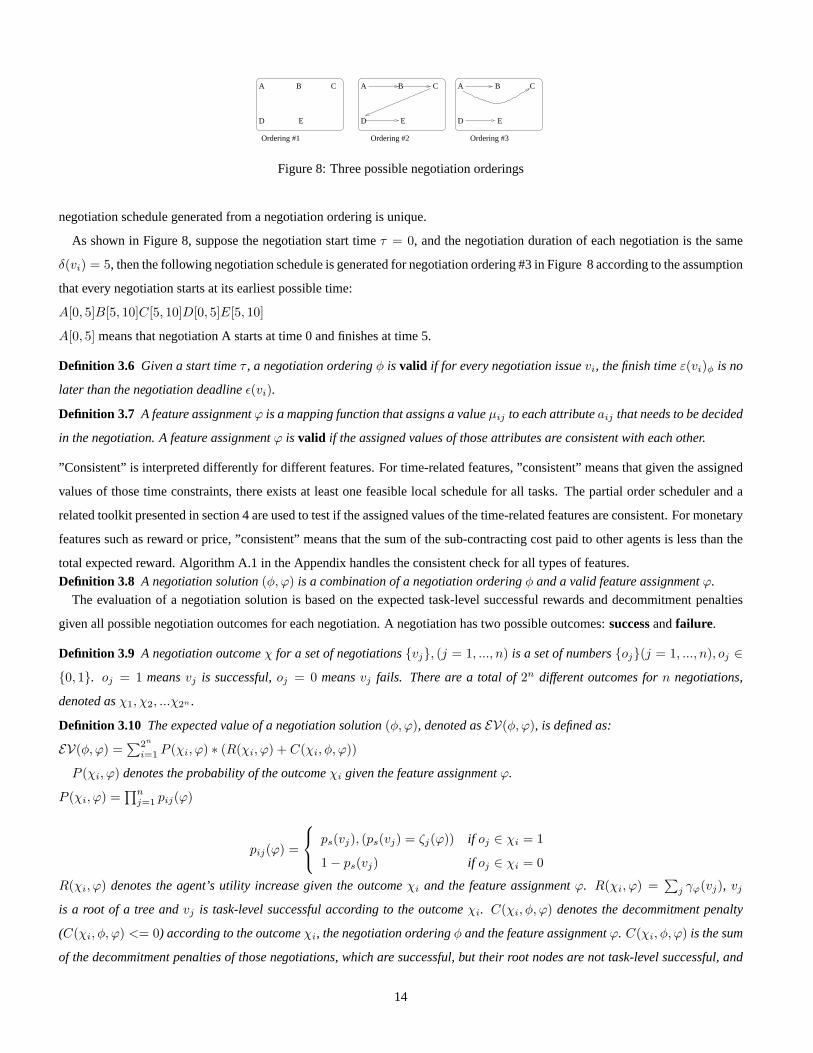
negotiation schedule generated from a negotiation ordering is unique.
As shown in Figure 8, suppose the negotiation start timeτ = 0, and the negotiation duration of each negotiation is the same
δ(vi) = 5, then the following negotiation schedule is generated for negotiation ordering #3 in Figure 8 according to the assumption
that every negotiation starts at its earliest possible time:
A[0, 5]B[5, 10]C[5, 10]D[0, 5]E[5, 10]
A[0, 5] means that negotiation A starts at time 0 and finishes at time 5.
Definition 3.6 Given a start timeτ , a negotiation orderingφ is valid if for every negotiation issuevi, the finish timeε(vi)φ is no
later than the negotiation deadlineε(vi).
Definition 3.7 A feature assignmentϕ is a mapping function that assigns a valueµij to each attributeaij that needs to be decided
in the negotiation. A feature assignmentϕ is valid if the assigned values of those attributes are consistent with each other.
”Consistent” is interpreted differently for different features. For time-related features, ”consistent” means thatgiven the assigned
values of those time constraints, there exists at least one feasible local schedule for all tasks. The partial order scheduler and a
related toolkit presented in section 4 are used to test if theassigned values of the time-related features are consistent. For monetary
features such as reward or price, ”consistent” means that the sum of the sub-contracting cost paid to other agents is lessthan the
total expected reward. Algorithm A.1 in the Appendix handles the consistent check for all types of features.Definition 3.8 A negotiation solution(φ, ϕ) is a combination of a negotiation orderingφ and a valid feature assignmentϕ.
The evaluation of a negotiation solution is based on the expected task-level successful rewards and decommitment penalties
given all possible negotiation outcomes for each negotiation. A negotiation has two possible outcomes:successandfailure .
Definition 3.9 A negotiation outcomeχ for a set of negotiations{vj}, (j = 1, ..., n) is a set of numbers{oj}(j = 1, ..., n), oj ∈
{0, 1}. oj = 1 meansvj is successful,oj = 0 meansvj fails. There are a total of2n different outcomes forn negotiations,
denoted asχ1, χ2, ...χ2n .
Definition 3.10 The expected value of a negotiation solution(φ, ϕ), denoted asEV(φ, ϕ), is defined as:
EV(φ, ϕ) =∑2n
i=1 P (χi, ϕ) ∗ (R(χi, ϕ) + C(χi, φ, ϕ))
P (χi, ϕ) denotes the probability of the outcomeχi given the feature assignmentϕ.
P (χi, ϕ) =∏n
j=1 pij(ϕ)
pij(ϕ) =
ps(vj), (ps(vj) = ζj(ϕ)) if oj ∈ χi = 1
1 − ps(vj) if oj ∈ χi = 0
R(χi, ϕ) denotes the agent’s utility increase given the outcomeχi and the feature assignmentϕ. R(χi, ϕ) =∑
j γϕ(vj), vj
is a root of a tree andvj is task-level successful according to the outcomeχi. C(χi, φ, ϕ) denotes the decommitment penalty
(C(χi, φ, ϕ) <= 0) according to the outcomeχi, the negotiation orderingφ and the feature assignmentϕ. C(χi, φ, ϕ) is the sum
of the decommitment penalties of those negotiations, whichare successful, but their root nodes are not task-level successful, and
14

such situations are unknown before these negotiation are started.C(χi, φ, ϕ) =∑
j βϕ(vj), vj represents every negotiation that
fulfills all the following conditions:
1. vj is successful according toχi;
2. the root of the tree thatvj belongs to isn’t task-level successful according toχi;
3. according to the negotiation orderingφ, there is no such negotiationvk existing that fulfills all the following conditions:
(a) vk andvj belong to the same tree;
(b) vk gets a failure outcome according to the outcomeχi;
(c) vk makes it impossible forroot(vj) to be task-level successful;
(d) the negotiation finish time ofvk is no later than the negotiation start time ofvj according to the negotiation orderingφ.
3.3 Description of a Heuristic Search Algorithm
Based on the above definition, we present an algorithm that find a nearly optimal (as we show in the experimental results)
negotiation solution for a multi-linked negotiation problemM = (V, E).
Given a multi-linked negotiation problemM = (V, E), the start time for negotiationτ , a set of valid feature assignments
ω = {ϕk}, k = 1, ...,m, the complete search algorithm evaluates each pair of negotiation ordering and valid feature assignment
(φi, ϕk), and then return the best one15. The exponential complexity of this complete algorithm prevents it from being used for
real-time applications when the number of negotiations andthe number of valid feature assignments are large; hence a heuristic
search algorithm has been developed.
The heuristic search for the near-optimal negotiation solution is broken into two parts. One is to find a near-optimal negotiation
schedule; the other one is to find a near-optimal feature assignment for a given negotiation schedule. The search for the optimal
negotiation schedule is based on a simulated annealing search. Given a negotiation orderingφ, randomly pick a PORe, if e ∈ Eφ,
remove it fromEφ; otherwise add it intoEφ16. A new negotiation orderingφnew is now generated. If the negotiation schedule
NS(φnew) is better thanNS(φ), move toφnew; otherwise, move toφnew with some probability less than 1. This probability
decreases exponentially with the “badness” of this move. Three heuristics have been added to this simulated annealing process:
1. Record the best negotiation schedule so far found. When thesearch process ends, return the best negotiation schedule ever
found rather than the current one.
2. Instead of randomly deciding whether to add a POR or removea POR, use a parameter (add por probability) to control
the probability of the operation “add” or “remove”. Actually, this parameter controls the tradeoff between sequencingversus
parallelizing the negotiation schedule (adding a POR forces two negotiations to be serialized).
3. Instead of completely randomly choosing a POR to change from current negotiation ordering, evaluate every PORe according
to how the value of the negotiation schedule changes by adding this PORe to an empty POR set. The probability of adding
PORe to the current POR set or removing PORe from the current POR set depends on this evaluation. A PORe with a higher
15If the set of valid feature assignments is a complete set of all possible validfeature assignments, this algorithm is guaranteed to find the best
negotiation solution. However, when the attributes have continuous value ranges, it is impossible to find all possible valid feature assignments.
We use a depth- first search (DFS) algorithm that searches over the entire value space for all undecided attributes by pre-defined search stepsize
and finds a set of valid feature assignments (See Appendix, Algorithm A.1).16The algorithm checks whether adding PORe to φ causes a circle. If so,e won’t be added, and the algorithm will randomly choose another
POR and continue.
15

positive evaluation has a higher probability of being added, and has a lower probability of being removed.
Consider an example with three negotiations A, B and C. Suppose the negotiation start timeτ = 0, and the negotiation duration
of each negotiation is the sameδ(vi) = 5, the evaluation of POR (A → B) is calculated as: the value of the negotiation
schedule:A[0, 5]B[5, 10]C[0, 5] minus the value of the negotiation schedule:A[0, 5]B[0, 5]C[0, 5].
The search for the near-optimal feature assignment is basedon a hill climbing search. Randomly pick another feature assignment
ϕk. If it is better than current one, move toϕk. After considering the characteristics of this problem, the following heuristics have
been added to this search process:
1. According to the generation process, the change of those valid feature assignments is continuous. Based on this observation, a
number of sample points with equal distance (the distance isadjustable, denoted assample step) in between can be selected
from all the valid feature assignments and evaluated. Hill climbing search then can be performed for each sample point.
2. Given current chosen feature assignment, the possible operations include: moving to left and moving to right. If there is a better
selection than current one, move to the better selection; otherwise the search stops and a local maxima is found.
3. Compare all local maxima and return the best one.
Both search algorithms are implemented with search limitation threshold: after certain amount of search effort, the algorithm
will stop and report the result. Experiments were performedto test how well these combined heuristic algorithms work, and as we
will describe in 6.1, the experimental work shows that the heuristic search algorithm finds solutions very close to the best solutions
found by the complete search algorithm with significantly less effort.
4 Partial Order Schedule and Related Algorithms
In this section, we will introduce a partial order schedulerwhich allows the agent to reason about the time-related constraints and
the flexibility associated with each negotiation issue. This toolkit is used by the agent to find valid feature assignments, which are
part of the input for the heuristic search algorithm described in Section 3.3.
4.1 Partial Order Schedule
A partial-order schedule is the basic reasoning tool that weuse for interrelated negotiations. Here we present the formalization
of the partial-order schedule and use examples to explain how it works for a multi-linked negotiation. Figure 9 shows thepartial-
ordered schedule generated for the example in Figure 4.
A partial order schedule17 represents a group of tasks with specified precedence relationships among them using a directed
acyclic graph:PS = (T,R). T = {t|tisatask}, where each vertex inT represents a task, andR = {(s, t)|s, t ∈ T )}, where
each edge(s, t) in R denotes the precedence relationship between tasks and taskt (P (s, t)), which means that tasks has to be
finished before taskt can be started.
A Task is represented as a node in the graph; it is the basic element of the schedule. A taskt needs a certain amount of
processing time, also referred as its duration (t.process time). A task can be a local task or a non-local task; a local task is
performed locally (i.e, taskGet SoftwareA and taskShippingComputerB) and a non-local task (i.e. taskGet Hardware A and
taskDeliver ComputerA) is performed by another agent; hence, it does not consume local process time. Thepretasks of taskt is
17In this paper, the term “partial order schedule” refers to a representation of a group tasks with specified precedence relationships, which also
includes the associated definitions in this section. The term “partial order scheduler” is used to refer to the procedure which actually produces
the partial order schedules for tasks, and a set of associated reasoning algorithms presented in Section 4.2.
16
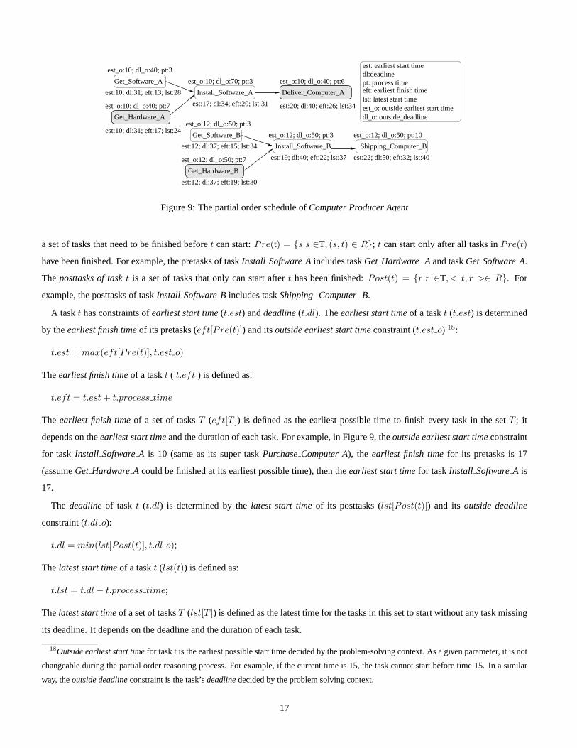
Get_Software_A
Install_Software_A
Install_Software_B Shipping_Computer_B
Get_Software_B
Deliver_Computer_A
est_o:10; dl_o:70; pt:3
est:17; dl:34; eft:20; lst:31est_o:10; dl_o:40; pt:7
est:10; dl:31; eft:17; lst:24
est:10; dl:31; eft:13; lst:28
est_o:10; dl_o:40; pt:6
est:20; dl:40; eft:26; lst:34
est_o:10; dl_o:40; pt:3
est_o:12; dl_o:50; pt:3
est:12; dl:37; eft:15; lst:34
est_o:12; dl_o:50; pt:7
est:12; dl:37; eft:19; lst:30
est_o:12; dl_o:50; pt:3
est:19; dl:40; eft:22; lst:37
est_o:12; dl_o:50; pt:10
est:22; dl:50; eft:32; lst:40
Get_Hardware_A
Get_Hardware_B
est: earliest start timedl:deadlinept: process time
dl_o: outside_deadlineest_o: outside earliest start time
eft: earliest finish timelst: latest start time
Figure 9: The partial order schedule ofComputer Producer Agent
a set of tasks that need to be finished beforet can start:Pre(t) = {s|s ∈T, (s, t) ∈ R}; t can start only after all tasks inPre(t)
have been finished. For example, the pretasks of taskInstall SoftwareA includes taskGet Hardware A and taskGet SoftwareA.
The posttasks of taskt is a set of tasks that only can start aftert has been finished:Post(t) = {r|r ∈T, < t, r >∈ R}. For
example, the posttasks of taskInstall SoftwareB includes taskShipping Computer B.
A taskt has constraints ofearliest start time(t.est) anddeadline(t.dl). Theearliest start timeof a taskt (t.est) is determined
by theearliest finish timeof its pretasks (eft[Pre(t)]) and itsoutside earliest start timeconstraint (t.est o) 18:
t.est = max(eft[Pre(t)], t.est o)
Theearliest finish timeof a taskt ( t.eft ) is defined as:
t.eft = t.est + t.process time
The earliest finish timeof a set of tasksT (eft[T ]) is defined as the earliest possible time to finish every task in the setT ; it
depends on theearliest start timeand the duration of each task. For example, in Figure 9, theoutside earliest start timeconstraint
for task Install SoftwareA is 10 (same as its super taskPurchaseComputer A), the earliest finish timefor its pretasks is 17
(assumeGet HardwareA could be finished at its earliest possible time), then theearliest start timefor taskInstall SoftwareA is
17.
The deadlineof task t (t.dl) is determined by thelatest start timeof its posttasks (lst[Post(t)]) and itsoutside deadline
constraint (t.dl o):
t.dl = min(lst[Post(t)], t.dl o);
The latest start timeof a taskt (lst(t)) is defined as:
t.lst = t.dl − t.process time;
Thelatest start timeof a set of tasksT (lst[T ]) is defined as the latest time for the tasks in this set to startwithout any task missing
its deadline. It depends on the deadline and the duration of each task.
18Outside earliest start timefor task t is the earliest possible start time decided by the problem-solving context. As a given parameter, it is not
changeable during the partial order reasoning process. For example, if the current time is 15, the task cannot start before time 15. In a similar
way, theoutside deadlineconstraint is the task’sdeadlinedecided by the problem solving context.
17

C
Get_Hardware_A
Deliver_Computer_A
Get_Hardware_B
[12, 37] [12, 26]
Get_Software_A
Install_Software_A
Get_Software_B
Install_Software_B Shipping_Computer_B
[22, 50]
[12, 26] [12, 37]
[10, 31] [10, 24]
[10, 31] [10, 24]
[17, 34] [24, 30] [20, 40] [30, 40]
[19, 40] [26, 44] [29, 50]
Purchase_Computer_B finish at time 50
Purchase_Computer_A finish at time 40
B
E
Figure 10: The consistent ranges for tasks in negotiation: Get HardwareA, Get HardwareB, and DeliverComputerA
Theflexibility of task trepresents the freedom to move the task around in this schedule.
F (t) = t.dl−t.est−t.process timet.process time
.
For example,F (Get Software A) = 40−10−33 = 9.
A feasible linear scheduleis a total ordered schedule of all tasks, that fulfills the following conditions:
• Each taskt takesn (n>=1, if t is interruptible; otherwise, n=1.) time periods (pti, i = 1, ...n ) for execution,∑
i pti =
t.processtime.
• All precedence relationships are valid.
• All earliest start time and deadline constraints are valid.
A partial-order schedule is avalid if and only if there exists at least one feasible linear schedule that can be produced from this
partial order schedule without additional constraints andwith the interruptible execution assumption19.
Without additional constraints and with the interruptibleexecution assumption, for a taskt with the range [est, dl], no matter
when taskt is executed during this range, if there exists at least one feasible linear schedule that can be produced from this partial
schedule, then the range [est, dl] for taskt is afree rangebecause taskt can be executed during any period in this range.
Without additional constraints and with the interruptibleexecution assumption, for a set of tasksti, (i = 1, 2, ..., n), with the
range[esti, dli], (i = 1, 2, ...n) respectively, no matter what timeti is executed during the range[esti, dli], if there exists at
least one feasible linear schedule that can be produced fromthis partial schedule, then the ranges[esti, dli], (i = 1, 2, ...n) for
tasksti, (i = 1, 2, ..., n) areconsistent ranges. Negotiation over tasksti, (i = 1, 2, ..., n) can be performed in parallel using
these consistent ranges without worrying about conflicts. Figure 10 shows the consistent ranges for the tasks in the supply chain
example. This means, the negotiation for task GetHardwareA, Get HardwareB, and DeliverComputerA can be performed in
19Partial order schedule is a representation and reasoning tool of a group of tasks and their interrelationships. It is not an executable schedule
for the agent. To translate a partial-order schedule to an executable linearschedule, there are two different assumptions: the task is interruptible
or non- interruptible. The interruptible execution assumption is that the agent can switch to another task during the execution of one task, and
it can switch back at some point and continue the execution of the incompletetask. The non-interruptible execution assumption does not allow
execution of a task to be split into parts. In this work we adopt the interruptibleexecution assumption, however, we also do not consider there is
cost for interrupting and resumption of a task.
18

Get_Software_A
[10, 24]
B E C
Get_Hardware_A Get_Hardware_B Deliver_Computer_A
10 13 13 16 24 27
Install_Software_A
[24, 30]
Install_Software_B
[12, 26]
Get_Software_B
40303027
Purchase_Computer_A finish at time 40 Purchase_Computer_B finish at time 40
[26, 44]
Shipping_Computer_B
[29, 50]
[10, 24] [12, 26] [30, 40] start time
consistent range
finish time
Figure 11: The feasible linear schedule for those tasks in Figure 10
parallel using the time range [10, 24], [12, 26] and [30, 40].Figure 11 presents a feasible linear schedule given these consistent
ranges. The two numbers in a box below a task represent the consistent range for this task, and the two numbers above a task
indicate the start time and the finish time for this task in onelinear schedule. It should be noticed that for each task the start time
and the finish time fall into its consistent range, they also can be moved freely during this range.
The partial order schedule work is related to the Graphical Evaluation and Review Technique(GERT) [8] which is used for
project scheduling and management. The major difference between the GERT work and ours is that the GERT work is not
oriented to negotiation; all activities are local and can bemanaged with authority. Thus, with GERT there is no reasoning about
free range, consistent ranges and schedule flexibility thatwe feel are critical for an agent to effectively manage multi-linked
negotiation. Without reasoning of these factors, it is difficult to negotiate efficiently on multiple related issues.
4.2 Algorithms
We have built the following algorithms to support the negotiation based on the partial order schedule. We only describe the
functions of these algorithms, the detailed processes are presented in [16]. The complexities of these algorithms are provided
accordingly,n represents the number of input tasks.
Algorithm 4.1 PropagateESTDL (Complexity:O(n2))
Given a set of tasks with the outside constraints of the earliest start times and deadlines, durations and precedence relationships,
this procedure finds the earliest start time (t.est) and the deadline (t.dl) for each taskt according to the definitions in Section 4.1.
Algorithm 4.2 Get Earliest Finish Time (Complexity:O(n2))
Given a set of tasksT , each task t has earliest start time (t.est) and its duration (t.process time), this procedure calculates the
earliest finish time of a set of tasksT (eft[T ]).
Algorithm 4.3 Get LatestStart Time (Complexity:O(n2))
Given a set of tasksT , each taskt has its deadline (t.dl) and its duration (t.process time), this procedure calculates the latest
start time of a set tasksT (lst[T ]).
Algorithm 4.4 FeasibleSchedule (Complexity:O(n4))
Given a partial order schedule (T, R), each task has its earliest start time and duration with respect to its pretask, posttask and its
outside constraints, this procedure generates a feasible linear schedule if the partial order schedule is valid; otherwise it reports
failure.
Theorem 4.1 If there exists a feasible linear schedule, the FeasibleSchedule algorithm can find one.
19

0.7
0.75
0.8
0.85
0.9
0.95
1
0 2 4 6 8 10 12 14
succ
ess
prob
abili
ty
flexibility
success probability depends on flexibility
Ps(B)=0.95*(2/pi)*atan(f(B)+2.5)Ps(C)=0.99*(2/pi)*atan(f(C)+5)
Figure 12: Success probability depends on flexibility
The proof of this theorem is presented in [16].
Besides Algorithm 4.4, we have also developed Algorithm 4.5to answer the question of whether a partial order schedule is
valid without trying to find a feasible linear schedule.
Algorithm 4.5 RangeEvaluation (Complexity:O(n2))
This procedure determines if a partial order schedule is valid.
The basic idea of Algorithm 4.5 is to check every possible time range[est, dl] by constructing all possible combinations of
every task’s earliest start time and deadline. For all tasksfalling into this range, if the sum of process times of these tasks is greater
than the time available(dl − est), there is no feasible linear schedule; otherwise, there exists a feasible linear schedule, because
every taskt can find a place between its earliest start time and itsdeadline.
This proves the following theorem:
Theorem 4.2 A partial order schedule is valid if and only if the procedure4.5 returns true.
Using the above procedure, we have constructed the following algorithm to find the free range of a non-local task used for the
negotiation.
Algorithm 4.6 Find NL Range (Complexity:O(n2))
Given a partial order schedule(T,R) containing a tasknlt, this procedure finds the largest free range for tasknlt.
If there is more than one non-local task, we need to sort them according to some characteristics (i.e. flexibility, importance,
difficulty of negotiation, etc.), and work on them one by one.When the FindNL range procedure works on one tasknlt i, the
range for those tasks before it (nlt 1, ...,nlt (i − 1)) has already been decided and cannot be changed. The range for those tasks
after it (nlt (i + 1), ...) are set to a range that is as small as possible, so as to allow this tasknlt i to have the most freedom.
All of the above algorithms and procedures provide a toolkitfor the agent to reason about its proposals and evaluate counter-
proposals from other agents.
5 Example
In this section, we demonstrate how the definition and the algorithm work on the supply chain examples in Figure 4.
20

Get_Software_A
Install_Software_A
Install_Software_B
Get_Software_B
[10, 31]
[17, 34]
[12, 37]
[19, 40] [22, 50]
Get_Hardware_A
[10, 31]
Get_Hardware_B
[12, 37]D Purchase_Computer_B finish at time 50
A Purchase_Computer_A finish at time 40
B
E
C
Deliver_Computer_A
[20, 40]
Shipping_Computer_B
Figure 13: Partial order schedule
To make the output easier to understand, only negotiation A (PurchaseComputerA), B (Get HardwareA) and C (De-
liver ComputerA) are considered in the following example. For incoming negotiation A, regular rewardr(A) = 19, the attribute
that needed to be decided is the promised finish timeft; the task-level successful reward depends on the promised finish timeft:
γ(v) = r(v) + e(v) ∗ (dl(v) − ft(v)).
For outgoing negotiation B and C, the attributes needed to bedecided are the start time (st) and the deadline (dl). It is assumed
that the negotiation durations are already known to the agent, δ(A) = 3, δ(B) = 4, δ(C) = 4. The negotiation start times
need to be decide by the agent as part of the problem of constructing a negotiation ordering. It is also assumed that the success
probability depends on the flexibilityf(v), which is calculated based on the time range(st(v), dl(v)) and the process timed(v)
(f(v) = dl(v)−st(v)−d(v)d(v) ):
ps(v) = pbs(v) ∗ (2/π) ∗ (arctan(f(v) + c))) 20
pbs is thebasic success probabilityof this negotiationv when the flexibilityf(v) is very large.c is a constant parameter used to
adjust the relationship. In this example, the following functions are used to determine the success probabilities for Band C:
ps(B) = pbs(B) ∗ (2/π) ∗ (arctan(f(B) + 2.5));
ps(C) = pbs(C) ∗ (2/π) ∗ (arctan(f(C) + 5)).
pbs(B) = 0.95, pbs(C) = 0.99.
The different constant parameters forps(B) (2.5) andps(C) (5) specify that issue C has a highersuccess probabilitythan issue
B given the same flexibility, as shown in Figure 12. The following parameters are randomly generated: the success probability of
A, the negotiation deadline, the early reward rate ofA, and the decommitment penalty.
For every attribute that needs to be decided: start time (st), deadline (dl) and the promised finish time (ft), the agent can find its
maximum possible range using the partial order schedule as shown in Figure 13. The agent searches over the entire possible value
space (Appendix, Algorithm A.1), and use the partial order schedule to test if a feature assignment is valid. A set of valid feature
assignments is found and used to find the optimal negotiationsolution combining ordering constraints and feature assignment.
20This function describes a phenomenon where initially the likelihood of a successful negotiation increases significantly as the flexibility
grows, and then levels off afterwards. This function mirrors our experience from the experiments in Section 6.3, which shows that after a certain
point, additional flexibility does not significantly improve the success probability. Obviously this function could be affected by the meta-level
information from the other agent.
21
Table 1 shows the output of the complete search algorithm (See Appendix, Algorithm A.3) on six different cases in Figure 5,
based on different negotiation deadlines, early reward rates and decommitment penalties. In both case 1 and case 2, the negotiation
deadlineε = 6 is used, which results in a negotiation ordering that has thethree negotiations performed in parallel. In case 2, A
has a higher earlier reward ratee(A), and all negotiations have lower decommitment penaltiesβ than in case 1, so the negotiation
solution in case 2 arranges task A to finish 21 time units earlier than the requested deadline, and earns an extra reward of 4.0. In
exchange, B and C have smaller flexibilitiesf(B) andf(C), hence lower success probabilityps(B) andps(C). In case 3 and
case 4, the negotiation deadlineε = 9. In case 3, A has a much lower success probabilityps(A) than in case 4, so negotiation A
is scheduled before negotiation B and C. In case 5 and case 6, the negotiation deadlineε = 11 and negotiation A, B and C are
sequenced according to the success probabilities; the negotiation with the lower success probability starts earlier.In case 6, A
has a higher earlier reward ratee(A), and all negotiations have lower decommitment penaltiesβ than case 5, so the negotiation
solution in case 6 arranges task A to finish 9 time units earlier than the requested deadline; this earns an extra of reward 1.3. In
exchange, B and C have smaller flexibilitiesf(B) andf(C) and hence lower success probabilitiesps(B) andps(C). It is also
important to notice that in all cases, B gets larger flexibility than C, but has a similar success probability to that of C. This occurs
because it is much easier for C to achieve a successful negotiation according to the function that defines the relationship between
the success probability and the flexibility. This result demonstrates that this type of reasoning is possible given the formal model
described in Section 3.
6 Experimental Work
We have implemented all the algorithms and reasoning tools described in previous sections. To evaluate how these mechanisms
work, we have built those agents that described in the supplychain scenario (Section 5). These agents are implemented using JAF
(Java Agent Framework) [4], which provides the basic functions such as communication and execution, for the agent, so wecan
focus on building the negotiation component. The experiments are performed in the multi-agent system simulator (MASS)[4],
which provides a concrete, re-runnable, well-defined environment to test multi-agent negotiation. We designed and performed
three sets of experiments for different purposes as described below.
6.1 Performance of Heuristic Algorithm
The first purpose is to test how well the heuristic algorithm works compared to the complete search algorithm. The experimental
setting is based on the example described in Section 5. New tasks were randomly generated with decommitment penaltyβ ∈
[0, 25], early finish reward ratee ∈ [0, 0.2], and deadlinedl ∈ [60, 70], and arrived at the contractee agents periodically. We use
the same task structures as described in Figure 4, tasks varywith randomly generated parameters. This scenario represents a class
of problems where one agent needs to deal with both directly-related and indirectly-related negotiation problems. Thedeadlines
of tasks are randomly generated from a range, which allows the agent to choose different negotiation orderings. The following
values (See algorithm A.4 for more details) were used in these experiments:add por probability = 0.55, TEMP MAX = 5;
TEMP STEP = 0.1; sample step = 10, search limit = 106.
Table 2 shows the performance of this heuristic search algorithm compared to the complete search algorithm. The qualityof the
negotiation solution found is very close to the best solution found by the complete search. This heuristic algorithm saves a large
amount of search effort compared to the complete search whenthe number of negotiations and the number of possible feature
assignments increase. The heuristic search spends more effort than the complete search when the search space is very small (with
22

Table 1: Examples of optimal negotiation solutions
ε v e(A) β et er f(v) ps(v)
negotiation early decommit Negotiation = dl − ft early reward flexibility success
deadline reward rate penalty Schedule = e(A) ∗ (dl − ft) probability
#1 A 0.012 22.2 A[0-3] 0 0 0.9
ε = 6 B 1.32 B[0-4] 3.0 0.84
C 1.32 C[0-4] 0.83 0.88
#2 A 0.189 1.95 A[0-3] 21 4.0 0.92
ε = 6 B 0.12 B[0-4] 1.0 0.78
C 0.12 C[0-4] 0.5 0.88
#3 A 0.117 16.6 A[0-3] 0 0 0.19
ε = 9 B 0.991 B[3-7] 3.0 0.84
C 0.99 C[3-7] 0.67 0.88
#4 A 0.006 16.6 A[4-7] 0 0 0.64
ε = 9 B 0.99 B[0-4] 2.43 0.83
C 0.99 C[0-4] 0.67 0.89
#5 A 0.043 17.7 A[0-3] 0 0 0.15
ε = 11 B 1.06 B[3-7] 2.43 0.83
C 1.06 C[7-11] 0.83 0.88
#6 A 0.142 12.6 A[8-11] 9 1.3 0.84
ε = 11 B 0.75 B[0-4] 1.43 0.80
C 0.75 C[4-8] 1.0 0.89
23

Table 2: Performance of heuristic search algorithm(NN: number of negotiations; NF: Number of valid feature assignments (the data points
are grouped according to NN and NF); Quality: the quality of the approachfound by the heuristic search compared to the best approach found
by the complete search (with quality normalized to 1.0); CS: the number of search steps of the complete search. HS: the number of search steps
of the heuristic search; Ratio: the ratio of heuristic search steps to completesearch steps. DS: Number of data samples)
NN NF Quality CS HS Ratio DS
3 [0, 50) 0.982 336 520 1.547 89
[50, 100) 1.000 832 590 0.709 3
5 [0, 50) 1.000 1759 1967 1.119 48
[50, 100) 0.998 3861 1766 0.457 6
6 [0, 50) 1.000 9353 1869 0.200 43
[50, 100) 0.998 19502 1734 0.089 111
[100, 150) 0.998 31086 1674 0.054 123
[150, 200) 0.996 44058 1674 0.038 108
[200, 250) 0.995 57253 1692 0.030 88
[250, 300) 0.994 70292 1670 0.024 57
[300, 350) 0.997 82736 1638 0.020 46
[350, 400) 0.995 95213 1644 0.017 28
[400, 450) 0.994 108185 1662 0.015 25
[450, 500) 0.998 121479 1667 0.014 17
a few negotiations and a few of feature assignments). This problem can be fixed by choosing the values of the search parameters
dynamically according to the size of current search space, instead of using the fixed values as we did in these experiments. For
example, when the number of negotiations (NN) and the numberof valid feature assignments (NF) is small, we can set the
search limit as a small number so that the search can stop earlier; becausea good-enough solution can be found with less search
effort in a small search space.
6.2 Different Negotiation Strategies
The second purpose is to test how different negotiation strategies affect the agent’s performance under multi-linked negotiation
situation. We compare the negotiation strategy generated from the reasoning based on the formalized model with some other sim-
pler strategies. Under this experimental setup, Computer Producer Agent needs to deal with multi- linked negotiationsrelated to
the incoming taskPurchaseComputerand the outgoing taskGet HardwareandDeliver Computer. The following three different
negotiation strategies were tested:
1. Sequenced Negotiation. The agent deals with the negotiations one by one, first the outgoing negotiations, then the incoming
negotiations. The finish time promised is the same as the deadline requested from the other agent, and the outgoing negotiations
get the largest possible flexibilities.
2. Parallel Negotiation. The agent deals with the negotiations in parallel. It arranges reasonable flexibility (1.5, inthis experiment)
for each outgoing task, and based on this arrangement, the finish time of the incoming task is decided and promised to the
contractee agent.
3. Decision-Based Negotiation. The agent deals with the negotiation as the best negotiation solution generated by the complete
search algorithm.
24

Table 3: Comparison of computer producer agent’s performance using different negotiation strategies
Policy Task Decommit Early Utility
Canceled Penalty Reward
Sequenced 37.25 73.82 0 358.09
Std.Dev. 2.6 11.8 0 57.4
Parallel 23.70 333.20 29.06 385.20
Std.Dev. 2.6 47.6 17.0 86.8
Decision-Based 25.78 56.65 185.79 779.16
Std.Dev. 2.4 23.5 47.8 62.3
The entire experiment contains 40 group experiments. Each group experiment has the system running for 1000 time clicks
for three times and each time Computer Producer Agent uses one of the three different approaches. During 1000 time clicks,
there are 60 new tasks received by Computer Producer Agent. Table 3 shows the comparison of Computer Producer Agent’s
performance using different strategies. When the agent usesthe sequenced negotiation strategy, more tasks are canceled because
of the missed negotiation deadlines. When the agent uses the parallel negotiation strategy, the agent pays a higher decommitment
penalty because the failure of the sub-contracted task prevents the incoming task to be task-level successful. The decision-
based approach is obviously better than the other two approaches21. It chooses a negotiation strategy dynamically according to
negotiation deadlines and other attributes. Under this experimental setup, it chooses the case where all negotiationsare performed
in parallel about 13% of the time; it chooses the case where all negotiations are performed sequentially about 38% of the time, and
the other times it chooses the case where some negotiations are performed in parallel. This strategy enables the agent toreceive
more early reward and pay fewer decommitment penalties.
The experimental result shows that in a multi-linked negotiation situation, it is very important for the agent to reasonabout the
relationship among different negotiations and make a reasonable decision about how to perform negotiation. This decreases the
likelihood of the need for decommitment from previously settled negotiations and increases the likelihood of utility gain.
6.3 Experiments on Flexibilities
The third purpose is to study how the different flexibility policies in negotiation, which involve different types of reasoning
strategies, affect the agent’s performance. The experimental environment is set up based on the scenario described in Figure
14. It is a simplified scenario from the example shown in Section 2. This scenario represents a class of problem where one
agent needs to deal with both directly and indirectly related negotiation problems. New tasks were randomly generated with
decommitment penalty ratep ∈ [0, 1], early finish reward ratee ∈ [0, 0.1], and deadlinedl ∈ [45, 105] (this range allows different
flexibilities available for those sub-contracted tasks), and arrived at the contractor agents periodically. The localscheduler of the
agent schedules all incoming new tasks occurring in a scheduling time window according to their earliest start times, deadlines,
process times and rewards and generates an agenda (such as agenda 2.1 on page 7). From this agenda, the agent can find the
21Using a t-test, with the 0.001 alpha-level, the following hypothesisHo is rejected: when using the decision-based approach, Computer
Producer Agent achieves an extra utility that is equal to 100% of the utility gained when using the sequenced negotiation strategy, and 78% of
the utility gained when using parallel negotiation strategy, compared to the hypothesisHa: when using the decision-based approach, Computer
Producer Agent achieves an extra utility that is more than 100% of the utility gained when using the sequenced negotiation strategy, and 78% of
the utility gained when using parallel negotiation strategy.
25

.
min
Purchuse_Computer
min
Sell_Computer
Install_Software
Get_Hardware
enables
enables
Get_Software
Shipping_Computerenables
Produce_Computer
Purchuse_Computer
Purchase_Parts
...... ......
Get_Hardware Purchase_Parts
Produce_Hardware Produce_Parts
Consumer Agent
Hardware Producer Agent
Computer Producer Agent
Figure 14: Three agents scenario
Get_Software_A
[10, 24]
Get_Hardware_A Get_Hardware_B Deliver_Computer_A
10 13 13 16 24 27
Install_Software_A Install_Software_B
[12, 26]
Get_Software_B
40303027
Purchase_Computer_B finish at time 40
Shipping_Computer_B
[10, 24] [12, 26] [27, 39]
[24, 27] [26, 30] [30, 40]
Purchase_Computer_A finish at time 39
B: process time 7 E: process time 7 C: process time 6
consistent range
start time finish time
Figure 15: The feasible schedule with flexibility of 1 for each non-local task
scheduled finish time of each task. It could continue the negotiation about these incoming tasks just based on the information
from this agenda without further reasoning about the detailed plan for each task (actually, that is what the agent does when using
the “Earliest-Finish-Time Policy” and the “Deadline Policy”). At the same time, if the local plan of these accepted tasks involves
any non-local tasknlt, then the FindNL Range procedure (Algorithm 4.6) is used to find the earliest start time and the deadline
of the tasknlt. The agent would then start negotiation with the other agentabout tasknlt based on this time range. The entire
experiment contains 32 group experiments. Every group experiment runs 3 times for 1000 time clicks each, each time usingone
of the three different polices (All agents use the same policy at the same time).
In this experiment,Computer Producer Agentneeds to deal with the multi- linked negotiations related tothe incoming task
PurchaseComputerand the outgoing taskGet Hardware. The following three different negotiation policies were tested:
1. Earliest Finish Time Policy: the agent finds the scheduled finish time of the task from its agenda and promises it as the finish
time in the contract with the intention of maximizing the early finish reward. In the example of Section 2.2,Computer Producer
Agentwill accept both taskPurchaseComputerA and taskPurchaseComputerB, with the promised finish time 26 and 46
respectively, according to agenda 2.1 on page 7.
2. Deadline Policy: The agent promises the finish time that is the same as thedeadlineof the task with no consideration of the
early finish reward. In the example of Section 2.2,Computer Producer Agentwill accept both taskPurchaseComputerA and
taskPurchaseComputerB, with the promised finish time 40 and 50 respectively, according to their deadline requests.
3. Flexibility Policy: the agent analyzes its detailed partial-order schedule. If non-local tasks are found, it arranges for reasonable
flexibility (1, in this experiment) for each non-local task,and based on this arrangement, the finish time of the incomingtask is
decided and promised to the contractee agent. In the exampleof Section 2.2,Computer Producer Agentwill accept both task
26

Table 4: Comparison of performance using different negotiation policies in multi- linked negotiation.
CPA: Computer Producer Agent; HPA: Hardware Producer Agent
Policy Tasks Tasks Tasks Early Decommit Early Utility
Received Accepted Canceled Finished Penalty Reward
CPA Earliest Finish Time Policy 60 59 27 33 123 283 391
CPA Deadline Policy 60 60 0.5 0 2.9 0 413
CPA Flexibility Policy 60 60 1.7 53 8.3 297 697
HPA Earliest Finish Time Policy 87 87 27 29 0 36 268
HPA Deadline Policy 84 84 9.6 0 0 0 256
HPA Flexibility Policy 87 87 11 17 0 32 294
PurchaseComputerA and taskPurchaseComputerB. The promised finish time for taskPurchaseComputerA is 39, and the
promised finish time for taskPurchaseComputerB is 40, according to the feasible schedule shown in Figure 15.
In all three cases above, the multiple negotiations are performed concurrently based on the free ranges found by the partial-order
scheduler. However, with the first two policies, the agent does not reason about the interaction among negotiations or manage the
flexibilities for each negotiation.
Table 4 shows the comparison of the agents’ performance using different policies. For theComputer Producer Agent(CPA),
who has multi- linked negotiations, the flexibility policy is obviously better than the other two policies; it gives the agent higher
utility because it generates more early reward and it causesfewer decommitment penalties22. For theHardware Producer Agent
(HPA), theEarliest Finish Time Policyand theFlexibility Policy make no difference in the agent’s decision making processes,
since the agent has no sub-contracted task that needs consideration. The reason that theEarliest Finish Time Policygenerates
less utility for HPA is that because theComputer Producer Agentcancels more task requests (because the finish times that the
Hardware Producer Agentcould provide are too late for CPA who also uses theEarliest Finish Time Policyat this time), and
hence theHardware Producer Agenthas fewer tasks to perform and gains less reward. Because theComputer Producer Agent
(CPA) is involved in the multi-linked negotiation, it pays lots of decommit penalties when it adopts theEarliest Finish Time Policy
when it finds that the finish time it promised can not be fulfilled. For theHardware Producer Agent(HPA), who does not need
sub-contract task to other agents, theEarliest Finish Time Policyproduces more utility than theDeadline Policybecause it brings
some early reward without paying any decommit penalty. These experiments shows that in a multi-linked negotiation situation, it
is very important for the agent to reason about the relationships among different negotiations and maintain reasonableflexibility
for them. This type of reasoning decreases the likelihood ofdecommitment from previously settled negotiations and thus gains
more utility.
22Using a t-test, with the 0.01 alpha-level, the following hypothesisHo is rejected: when using the flexibility policy,Computer Producer
Agentachieves an extra utility that is equal to 64% of the utility gained when using theEarliest Finish Time Policy, compared to the hypothesis
Ha: when using the flexibility policy,Computer Producer Agentachieves an extra utility that is more than 64% of the utility gained when using
theEarliest Finish Time Policy.
27
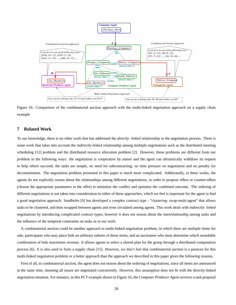
Consumer Agent
Purchase_Parts
Hardware Producer Agent Transporter Agent
Deliver_ComputerGet_Hardware
Computer Producer Agentprocess−time: 7
Purchase_Computer
Get_Hardware
Produce_Computer
Get_SoftwareInstall_Software
enablesprocess−time: 3
process−time: 3
enables
enables
process−time: 6
Deliver_Computer
and
and
Can you do it during time 10−25 and within cost $110?
C
A
I can do it in one of the following ways:
B
I can do it in one of the following ways:
{$100, 10−17}, {$105 11−18}
{$103, 12−19} ......,{$80, 30−37}......
{$5, 15−21}, {$6 16−22},
{$7, 17−23} ......,{$4, 30−36}......
Can you do it during time 28−40 and within cost $8?
Combinatorial Auction Approach
Multi−linked Negotiation Approach
Combinatorial Auction Approach
Figure 16: Comparison of the combinatorial auction approach with the multi-linked negotiation approach on a supply chain
example
7 Related Work
To our knowledge, there is no other work that has addressed the directly- linkedrelationship in the negotiation process. There is
some work that takes into account theindirectly-linkedrelationship among multiple negotiations such as the distributed meeting
scheduling [12] problem and the distributed resource allocation problem [2]. However, those problems are different from our
problem in the following ways: the negotiation is cooperative by nature and the agent can altruistically withdraw its request
to help others succeed; the tasks are simple, no need for subcontracting; no time pressure on negotiation and no penalty for
decommitment. The negotiation problem presented in this paper is much more complicated. Additionally, in these works,the
agents do not explicitly reason about the relationships among different negotiations, in order to propose offers or counter-offers
(choose the appropriate parameters in the offer) to minimize the conflict and optimize the combined outcome. The ordering of
different negotiations is not taken into consideration in either of these approaches, which we feel is important for theagent to find
a good negotiation approach. Sandholm [9] has developed a complex contract type - ”clustering- swap-multi-agent” thatallows
tasks to be clustered, and then swapped between agents and even circulated among agents. This work deals withindirectly- linked
negotiations by introducing complicated contract types, however it does not reason about the interrelationship amongtasks and
the influence of the temporal constraints on tasks as in our work.
A combinatorial auction could be another approach to multi-linked negotiation problem, in which there are multiple items for
sale, participants who may place bids on arbitrary subsets of those items, and an auctioneer who must determine which awardable
combination of bids maximizes revenue. It allows agents to select a shared plan for the group through a distributed computation
process [6]. It is also used to form a supply chain [15]. However, we don’t feel that combinatorial auction is a panacea forthis
multi-linked negotiation problem or a better approach thanthe approach we described in this paper given the following reasons.
First of all, in combinatorial auction, the agent does not reason about the ordering of negotiations, since all items areannounced
at the same time, meaning all issues are negotiated concurrently. However, this assumption does not fit with the directly-linked
negotiation situation. For instance, in this PCT example shown in Figure 16, theComputer Producer Agentreceives a task proposal
28

PurchaseComputer(A) from theConsumer Agent. To accomplish this task, theComputer Producer Agentneeds to subcontract
taskGet Hardware (B) and taskDeliver Computer(C). If we put this example into the combinatorial auction framework, we
will find that there is no way that these three negotiation issues A, B, and C can be performed concurrently without conflict.
Using the combinatorial auction model with time constraints [6], theComputer Producer Agentneeds to first announce the two
tasksGet HardwareandDeliver Computer, and wait for other agents to bid for these two tasks, and thenselect the combined
bids with consistent time constrains and minimized cost. Based on these selected bids, theComputer Producer Agentcan go
back to negotiate with theConsumer Agent. Using this model, the ordering of negotiations A, B and C is always (B,C)→ A.
This could be a solution, but by no means to be the best solution under all circumstances. As we have analyzed before and
also as the experimental results shown, the agent should dynamically choose the negotiation ordering based on the negotiation
deadlines, decommiment penalties, the estimations of successful probabilities, and other environmental context so as to maximize
the expected utility. However, the combinatorial auction model neither reasons about these attributes nor provides the agent with
the flexibility to choose from different negotiation orderings. This limitation prevents the agent from finding a betternegotiation
solution.
Secondly, the agent using a combinatorial auction model neither actively reasons about the interrelationships among these
related negotiation nor tries to direct the negotiations toa hopefully optimal solution, but just waits passively and select the solution
from whatever is available, which does not guarantee findinga (good) solution. Let’s continue with the previous example, using the
combinatorial auction model, theComputer Producer Agentsimply announces the two tasksGet HardwareandDeliver Computer
and waits for the other agents’ bids. When theHardware Producer Agentand theTransporter Agentconstruct their bids for these
two tasks respectively, they have no idea of how these two tasks relate to each other, all they can do is to construct the bids
based on their local problem solving context. Suppose basedon the ”first come, first serve” rule, these two agents arrangethese
new tasks after their current tasks. Assume that the bid fromtheHardware Producer Agentis ”Get Hardware, cost$100, time
range: 10-17” based on its current task finishes at 10 and it takes 7 time units to perform taskGet Hardware, and the bid from
the Transporter Agentis ”Deliver Computer, cost$5, time range: 15-21” based on its current task finishes at 15 and it takes 6
time units to perform taskDeliver Computer. However, based on these two bids, theComputer Producer Agentcannot find a
consistent solution because there is no time left for the task Install Software. Actually the solution does exist if theTransporter
Agentwould leave some slack time before starting taskDeliver Computer. TheTransporter Agentdoes not have the necessary
information that leads to this decision. To solve this problem in combinatorial auction, it can be requested that the contractee agent
generate all possible bids and send them all to the contractor agent. However, this solution causes large amount of communication
(as shown in Figure 16, upper part), and large number of bids makes the winning-determination (WD) process more difficult
and time-consuming23. This example shows that combinatorial auction is not a suitable model for multi-linked negotiation with
complicated task relationships. In comparison, in our approach (as shown in Figure 16, lower part), theComputer Producer Agent,
who has the most complete information, leads the negotiation by analyzing the relationships among negotiations and arranging
appropriate time ranges for related subjects in negotiation, which resulting in a more efficient negotiation process and a better
solution in the end.
Thirdly, the general winning-determination problem for combinatorial auction is NP-complete [3]. Current WD algorithms[11,
23There has been some recent work on preference elicitation[1] that potentially could reduce the number of bids need to be sent. However, it
is our intuition that to make this preference elicitation process successful, itwould need the similar type of reasoning process as shown in our
work.
29

3] are based on depth-first search and using different types of heuristics. So, from the computational complexity perspective,
combinatorial auction and our approach are at the same levelcomplexity.
The above analysis shows that combinatorial auction could be another approach to multi-linked negotiation, but it has limitation
that does not permit efficient management of the negotiations where there are complex relationships. The approach in this paper
provides a more general model and solution to multi- linked negotiation problem.
8 Summary
In this paper, we defined the multi-linked negotiation problem and demonstrate how an agent could deal with the multi-linked
negotiation problem. Multi-linked negotiation deals withmultiple negotiations, where these negotiations are interconnected - the
negotiation over one issue affects other negotiations. To solve a multi-linked negotiation problem, the agent needs tofind out
in what order the negotiations should be performed, and how to negotiate on each issue to avoid conflict among them. First,
we construct a partial order schedule, which allows the agent to reason about time-related constraints and flexibility on each
issue. This reasoning process is important for the agent to perform conflict-free negotiation and manage flexibility in negotiation.
Furthermore, we presented a formalized model of the multi-linked negotiation problem that enables the agent to represent and
reason about the relationships among different negotiations explicitly. Using this model, a heuristic search algorithm is developed
to that finds the nearly optimal approach in reasonable time.Experimental work shows that this management technique for
multi-linked negotiation leads to improved performance over other simpler approaches.
In this work, we model the success probability as a function that depends on a set of features, but we have not worked out how
the agent can construct such a function. In the future, we’d like to use meta-level information and learning technologies for an
agent to construct and adjust the structure of this function. Also, the model and the algorithm presented here are for individual
agents, to extend this model to a multi-agent system is another direction of our future work. Additionally, in this work,the result
of the negotiation is limited to two outcomes: “success” or “fail”. Actually, when negotiation is successful, there arepotentially
many different outcomes depending on the parameters in the commitment. such as different promising finish times. Depending
upon the different outcomes, the agent can adjust its other negotiations that are related to this negotiation. The negotiation process
can be modeled as a Markov decision process, and the negotiation solution can be generated as a policy: perform the negotiation
according to the results of the previous negotiations. Thisis another direction of our future work.
References
[1] W. Conen and T. Sandholm. Preference elicitation in combinatorial auctions: Extended abstract. InACM Conference on Electronic
Commerce (ACM-EC), Tampa, FL, October 14-17 2001.
[2] M. Frank, A. Bugacov, J. Chen, G. Dakin, P. Szekely, and B. Neches. The marbles manifesto: A definition and comparison of cooper-
ative negotiation schemes for distributed resource allocation. InAAAI Fall 2001 Symposium on ”Negotiation Methods for Autonomous
Cooperative Systems,”, 2001.
[3] Y. Fujishima, K. Leyton-Brown, and Y. Shoham. Taming the computational complexity of combinatorial auctions: Optimal and approxi-
mate approaches. InProceedings of International Joint Conference on Artificial IntelligenceIJCAI’99, Stockholm, Sweden, 1999.
[4] B. Horling, R. Vincent, and V. Lesser. Multi-agent system simulation framework. In16th IMACS World Congress 2000 on Scientific
Computation, Applied Mathematics and Simulation. EPFL, August 2000.
[5] B. Horling, R. Vincent, R. Mailler, J. Shen, R. Becker, K. Rawlins, and V. Lesser. Distributed sensor network for real time tracking. In
Proceedings of the 5th International Conference on Autonomous Agents, pages 417–424, Montreal, June 2001. ACM Press.
30

[6] L. Hunsberger and B. J. Grosz. A combinatorial auction for collaborative planning. InProceedings of the Fourth International Conference
on Multi-Agent Systems (ICMAS-2000), 2000.
[7] J. J. Moder, C. R. Phillips, and E. W. Davis.Project management with CPM, PERT and precedence diagramming. Blitz Pub Co, 1995.
[8] A. Pritsker. Gert networks (graphical evaluation and review technique. The Production Engineer, 1968.
[9] T. Sandholm and V. Lesser. On automated contracting in multi-enterprise manufacturing. InProceedings of the Improving Manufacturing
Performance in a Distributed Enterprise: Advanced Systems and Tools.
[10] T. Sandholm and V. Lesser. Issues in automated negotiation and electronic commerece: Extending the contract net framework. In
Proceedings of the First International Conference on Multi-Agent Systems (ICMAS95), 1995.
[11] T. Sandholm and S. Suri. Improved algorithms for optimal winner determination in combinatorial auctions and generalizations. InNational
Conference on Artificial Intelligence (AAAI), 2000.
[12] S. Sen and E. H. Durfee. A formal study of distributed meeting scheduling.Group Decision and Negotiation, 7:265–289, 1998.
[13] R. G. Smith. The contract net protocol: High-level communication and control in a distributed problem solver.IEEE Transactions on
Computers, 1980.
[14] T. Wagner and V. Lesser. Evolving real-time local agent controlfor large-scale mas. In J. Meyer and M. Tambe, editors,Intelligent Agents
VIII (Proceedings of ATAL-01), Lecture Notes in Artificial Intelligence. Springer-Verlag, Berlin, 2002.
[15] W. Walsh, M. Wellman, and F. Ygge. Combinatorial auctions for supply chain formation. InSecond ACM Conference on Electronic
Commerce, 2000.
[16] X. Zhang.Sophisticated Negotiation In Multi-Agent Systems. PhD thesis, University of Massachusetts Amherst, 2002.
[17] X. Zhang, V. Lesser, and R. Podorozhny. New results on cooperative, multistep negotiation over a multi-dimensional utility
function. In AAAI Fall 2001 Symposium on ”Negotiation Methods for Autonomous Cooperative Systems”, pages 1–10, 2001.
http://mas.cs.umass.edu/x̃qzhang/pub/NewResultNeg-01.ps.
A Appendix
Algorithm A.1 Find a set of valid feature assignments.
Input: M = (V, E).
For each attributeaij , if aij is already decided, the value ofaij is decided value(aij);
if aij is undecided, the maximum possible range foraij is: [min value(aij),max value(aij)],
the search step size:stepij .
Output: a set of valid feature assignmentsω.
Generate the possible value setΨij for attributeaij ;
If aij is already decided,Ψij = {decided value(aij)};
Elsex = min value(aij);
Repeat
addx to Ψij ;
x = x + stepij ;
Until x > max value(aij)
Generate all possible feature assignmentsϕk based on the possible values inΨij ;
If valid(ϕk), addϕk into ω;
Returnω;
Algorithm A.2 Evaluate a negotiation schedule with all possible feature assignments and findthe best feature assignments and the best value.
Input: negotiation scheduleφ, a set of valid feature assignmentsω = {ϕk}, k = 1, ..., m.
Output: the best value with the best feature assignment.
31

begin
for(i=0; i <=m; i+=sample step)
addϕi to searchset;
for eachϕi in searchset
for(t=0; t<searchlimit; t++)
if(EV(φ, ϕi+1) > EV(φ, ϕi))
i=i+1;
else if(EV(φ, ϕi−1) > EV(φ, ϕi))
i=i-1;
else
break;
if(EV(φ, ϕi) > bestvalue)
bestvalue =EV(φ, ϕi);
bestassignment = i;
return(bestvalue,bestassignment);
end
Algorithm A.3 Complete search: Find the best negotiation strategy.
Input: M = (V, E), the start time for negotiationτ , a set of valid feature assignmentsω = {ϕk}, k = 1, ..., m.
The complete search algorithm evaluates each pair of negotiation orderingand valid feature assignmentEV(φi, ϕk), then return the best one.
Output:the best negotiation strategy.
Generate all valid negotiation orderings{φi};
bestvalue = minimumvalue;
bestordering = null;
bestassignment = null;
for each negotiation orderingφi
for each valid feature assignmentϕk
if EV(φi, ϕk) > best value
bestvalue =EV(φi, ϕk);
bestordering = φi;
bestassignment =ϕk;
return (bestordering, bestassignment)
Algorithm A.4 Heuristic search: Find the best negotiation strategy.
Input: M = (V, E), the start time for negotiation (τ ), a set of valid feature assignmentsω = {ϕk}, k = 1, ..., m, the probability to add a
por:add por probability. TEMPMAX, TEMPSTEP: search parameters.
Output:the best negotiation strategy.
begin
Generate all possiblePORs = {(vi, vj)|vi, vj ∈ V }
total value = 0;
total inversevalue = 0;
basevalue = evaluateschedule(NS(V, ∅), ω);
for each por∈ PORs
φ(por) = (V, por)
por.value = evaluateschedule(NS(φ(por)), ω).value - basevalue;
32

por.inversevalue = 1.0 / por.value;
total value = total value + por.value;
total inversevalue = total inversevalue + por.inversevalue;
for each por∈ PORs
por.in probability = por.value/totalvalue;
por.out probability = por.value/totalinversevalue;
for(t = TEMP MAX; t >= 0; t− = TEMP STEP )
generate a random numberr between[0, 1];
if( r < add por probability)
choose a por e from PORs/currentordering
according to inprobability
newordering = currentordering∩e
else
choose a por e from currentordering according to
out probability
newordering = currentordering - e
evaluationresult = evaluateschedule(NS(φ(new ordering)), ω);
changevalue = evaluationresult.value - currentvalue;
if (change value > 0||random < e−change value/t)
current value = evaluationresult.value;
current assignment = evaluationresult.assignment;
current ordering = newordering;
if (change value > best value)
bestvalue = currentvalue ;
bestassignment = currentassignment;
bestordering =currentordering;
return (bestordering, bestassignment);
end
33