effect of pipe rotation on casing pressure within mpd
TRANSCRIPT

Louisiana State UniversityLSU Digital Commons
LSU Master's Theses Graduate School
3-11-2018
Effect of Pipe Rotation on Casing Pressure WithinMPD ApplicationsZahrah Ahmed Al MarhoonLouisiana State University and Agricultural and Mechanical College, [email protected]
Follow this and additional works at: https://digitalcommons.lsu.edu/gradschool_theses
Part of the Petroleum Engineering Commons
This Thesis is brought to you for free and open access by the Graduate School at LSU Digital Commons. It has been accepted for inclusion in LSUMaster's Theses by an authorized graduate school editor of LSU Digital Commons. For more information, please contact [email protected].
Recommended CitationAl Marhoon, Zahrah Ahmed, "Effect of Pipe Rotation on Casing Pressure Within MPD Applications" (2018). LSU Master's Theses.4630.https://digitalcommons.lsu.edu/gradschool_theses/4630

EFFECT OF PIPE ROTATION ON CASING PRESSURE WITHIN MPD APPLICATIONS
A Thesis
Submitted to the Graduate Faculty of the Louisiana State University and
Agricultural and Mechanical College in partial fulfillment of the
requirements for the degree of Master of Science
in
The Department of Petroleum Engineering
by
Zahrah Ahmed Al Marhoon B.S., Texas A&M University, 2012
May 2018

ii
This work is dedicated to my family and friends. Especially my husband who’s without his
support, this would not have been possible.
This is for you Hussain
This is for you Rihana.

iii
Acknowledgments
First, I would like to extend my deepest gratitude to my committee chair, Dr. Babak Akbari, for
his continuous support throughout the making of this work. I appreciate his readiness to answer
all questions quickly and for being considerate and accommodating to my personal
circumstances.
I would also like to acknowledge my committee members: Dr. Tyagi, Dr. Almeida and Mr. Erge.
I am gratefully indebted to them for their valued comments on this thesis.
Finally, I would like to express my profound thankfulness to my parents, husband, family and
friends for their faith in me and their non-stop support throughout this and all other journeys.

iv
TABLE OF CONTENTS
ACKNOWLEDGMENTS ......................................................................................................... iii
NOMENCLATURE .................................................................................................................. vi
ABSTRACT ............................................................................................................................ viii
CHAPTER 1: INTRODUCTION AND LITERATURE REVIEW .............................................. 1 1.1 Introduction to Managed Pressure Drilling ....................................................................... 1 1.2 Well Control Methods and MPD Well Control ................................................................. 4 1.3 Pipe Rotation and Eccentricity Effect on Frictional Pressure Loss .................................. 16 1.4 Two Phase Flow in Wellbore with Gas Kick .................................................................. 17
CHAPTER 2: STATEMENT OF PROBLEM AND APPROACH ............................................ 21 2.1 Statement of Problem ..................................................................................................... 21 2.2 Approach ....................................................................................................................... 22 2.3 Real Scale Experiments in LSU#2 Well ......................................................................... 24 2.4 Pipe Rotation Frictional Pressure Loss Effect Correlations ............................................. 27
CHAPTER 3: ANALYSIS OF FRICTIONAL PRESSURE CHANGES ON CASING PRESSURE CAUSED BY PIPE ROTATION IN OIL BASED MUDS USING DISSOLVED GAS MODEL ........................................................................................................................... 39 3.1 Overview ....................................................................................................................... 39 3.2 Dissolved Gas Model for Oil Based Muds ...................................................................... 40 3.3 Example of Full-Scale Data Output (OBM) .................................................................... 41 3.4 Pipe Rotation Effect on Casing Pressure in OBM Using Dissolved Gas Model .............. 42 3.5 Validity of the Dissolved Gas Model in OBM ................................................................ 47 3.6 Summary of the Results and Conclusion of Dissolved Gas Model for OBM ................... 48
CHAPTER 4: ANALYSIS OF FRICTIONAL PRESSURE CHANGES ON CASING PRESSURE CAUSED BY PIPE ROTATION IN WATER BASED MUDS USING SINGLE BUBBLE MODEL ................................................................................................................... 50 4.1 Overview ....................................................................................................................... 50 4.2 Single Bubble Model for Water Based Muds .................................................................. 51 4.3 Example of Full Scale Data Output (WBM) ................................................................... 54 4.4 Pipe Rotation Effect on Casing Pressure in WBM Using Single Bubble Model .............. 55 4.5 Summary of the Results and Conclusion of Single Bubble Model for WBM .................. 60

v
CHAPTER 5: VALIDITY OF SINGLE BUBBLE MODEL AND GAS DISTRIBUTION ....... 62 5.1 Overview ....................................................................................................................... 62 5.2 Gas Kick Distribution in Wellbore ................................................................................. 63 5.3 Pipe Rotation Effect on Gas Distribution ........................................................................ 66 5.4 Conclusion on Validity of the Single Bubble Model ....................................................... 74
CHAPTER 6: ANALYSIS OF CASING PRESSURE CHANGES CAUSED BY GAS BUBBLE BREAKAGE USING DISPERSED BUBBLE MODEL ........................................................... 76 6.1 Overview ....................................................................................................................... 76 6.2 Dispersed Bubble Model for WBM ................................................................................ 76 6.3 Conclusion of Dispersed Bubble Model ......................................................................... 83
CHAPTER 7: SUMMARY, APPLICATIONS, AND RECOMMENDATIONS FOR FUTURE RESEARCH ............................................................................................................................. 85 7.1 Summary ....................................................................................................................... 85 7.2 Application .................................................................................................................... 88 7.3 Recommendations for Future Research .......................................................................... 91
BIBLIOGRAPHY .................................................................................................................... 93
APPENDIX A: REAL SCALE EXPERIMENTS DATA OUTPUT .......................................... 96
APPENDIX B: COPYRIGHT MATERIAL .............................................................................. 98
APPENDIX C: FRICTIONAL PRESSURE CALCULATION EXAMPLE .............................. 99
VITA . .................................................................................................................................... 102

vi
NOMENCLATURE
Aann Area of the Annulus
BHP Bottom Hole Pressure
BOP Blowout Preventer
CBHP Constant Bottom Hole Pressure
DC Drill Collar
Dg Location of gas at a certain time step
DFD Dynflodrill
Di Inner Diameter of Annulus
Do Outer Diameter of Annulus
DP Drill pipe
ECD Equivalent Circulating Density
HP Hydrostatic Pressure
K Consistency index of mud
L" Length of the gas section
L$ length of the mud section below the gas with pump rate
L% length of the mud section above the gas with the increased mud rate
m Flow behavior index
𝑀𝑀 Molecular Mass of air
MPD Managed Pressure Drilling
MW Mud Weight (Density)
N Generalized flow behavior Index
OBM Oil Based Mud
P Pressure
𝐶𝑃)*+ Casing pressure with Rotation
C-./.01 Casing pressure without rotation
𝐹𝑃 Frictional pressure loss including pipe rotation effect Pt Pressure of gas at the top of the well
PV Plastic Viscosity
PWD Pressure While Drilling
R Universal Gas Constant
Ri Radius of Inner Pipe, Di/2
Ro Radius of Outer Pipe, Do/2
RPM Rotation Per Minute
𝑆𝐺 Specific Gravity of gas
T Absolut Temperature
t the time step
t₀ Time at which the gas exited the well
Ta Taylor number, Dimensionless
TD Total Depth
v Axial Velocity, m/s
v789: peak velocity of the mud taken from OBM velocities
v Velocity

vii
V Volume
Vb Volume of kick at the bottom of the well
ve The extra velocity of gas added to peak velocity of liquid
Vt Volume of gas at the top of the well.
WBM Water Based Mud
WCM Well Control Matrix
YP Yield Point
ω Rotational Speed
𝛽 Void fraction of gas of annulus
𝜏= yield stress of mud
𝛾? Axial Shear rate , s-1
𝛾@ Radial Shear rate, s-1
𝜌" Gas density BC×++×*)E
𝜌FGH Density of the mixture in the dispersed gas model
𝜌FIJ Mud density
𝜆 FIJ Void fraction of mud in the dispersed gas model
µapp Apparent Viscosity

viii
ABSTRACT
Well control is one of the most crucial sectors in drilling engineering. Human lives and safety
depend on the correct execution of the engineering design. Managed Pressure Drilling (MPD) is
a new technology that has recently emerged in the oil and gas industry. It has special well control
abilities supported by the RCD to continue drilling or carry operations that involve pipe rotation,
while circulating out a gas kick. This thesis examines the effect of pipe rotation on casing
pressure profiles within MPD kick circulation application. The analysis was carried on real scale
kick experiments. These experiments were carried in a controlled environment that mimicked
downhole conditions with a gas influx entering the wellbore. Both water based mud and oil
based mud were evaluated. Then, the real scale tests analysis was coupled with the effect of pipe
rotation through the application of correlations. The correlations estimate the change in frictional
pressure loss in the annuls for non-Newtonian fluids with pipe rotation. A study of the effect of a
larger size gas bubble breakage into smaller size bubbles on the maximum anticipated casing
pressure is also included in this research.
The thesis was divided into three models: (1) dissolved gas model in OBM. (2) single bubble
model in WBM. (3) dispersed bubble model in WBM. The first two models studied the effect of
frictional pressure changes on the anticipated casing pressure. The dispersed bubble model
studies the effect of breaking the gas bubble into many very small bubbles. The practical
outcome is to further the precision of the estimation of downhole pressure limits since MPD
address narrow fracture-pore pressure window and to find if casing pressure changes would have
any effect on the RCD rating selection and if the rotation can be safely conducted.

1
CHAPTER 1: INTRODUCTION AND LITERATURE REVIEW
1.1 Introduction to Managed Pressure Drilling
Drilling Engineers deal with several challenges with each well they plan. New technologies have
emerged in the oil and gas industry to address these challenges. These technologies allow drilling
engineers to carefully design and efficiently carry the operation. One of these new technologies
is managed pressure drilling (MPD).
1.1.1 Definition of managed pressure drilling
The IADC defines MPD as “an adaptive drilling process used to precisely control the annular
pressure profile throughout the wellbore. The objectives are to ascertain the downhole pressure
environment limits and to manage the annular hydraulic pressure profile accordingly.”
The term MPD was used for the first time in Amsterdam Drilling Conference in 2004. MPD is
especially important for the application of narrow operational window between pore pressure and
fracture pressure. MPD introduced for a long time as a method to overcome some industry
challenge to make drilling in more difficult environment visible such as pressure profile
uncertainty, ballooning and loss circulation. Casing string failure of reaching to total depth due to
pressure regime and low ROP are just examples of the well challenges that MPD could help in
1.1.2 Importance of MPD
MPD has had a growing demand in the industry for many reasons. 70% of the hydrocarbon
resource available offshore are not economically drillable using conventional methods (Ian
2004). MPD allowed to drill in a well that could not be drilled otherwise. In a survey done for
more than 600 SPE members worldwide, the results showed 25% of the wells that were not able

2
to be drilled with the old technology (Fig 1.1), and that MPD technology opens the possibility of
drilling those wells safely (Jacobs and Donnelly 2011). In the Gulf of Mexico, MPD
implementation decreased the drilling cost by $25-40 per foot (Rehm et al. 2008).
Figure 1. 1: Importance of MPD survey (Jacobs and Donnelly 2011) 1
1.1.3 Types of MPD Operations and Equipment
There are various types of operation for MPD:
1) Constant Bottom Hole Pressure (CBHP) that allow to reduce the NPT by enabling fewer
and deeper casing string especially where the pore pressure and fracture pressure window
is narrow. In this method RCD is implemented to control the bottom hole pressure by
applying backpressure to the annulus even while circulating.
2) Pressurized Mud Cap Drilling (PMCD) allow more drilling through increasing rate of
penetration and decrease in flat time in drilling in a loss circulation environment.
3) Dual Gradient (DG) enable drilling to target depth with the desired hole size, especially
in deep water drilling (“Introduction to Managed Pressure Drilling with MicroFluxTM
Control” 2012).
1 Copyright permission included in appendix B
3
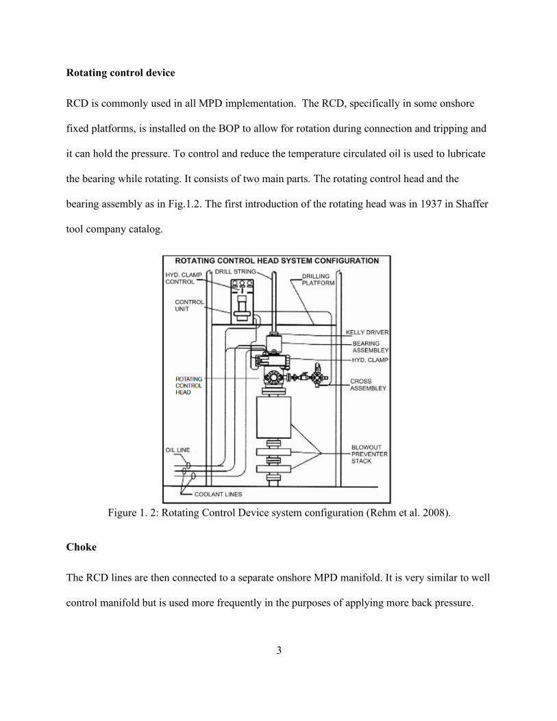
Rotating control device
RCD is commonly used in all MPD implementation. The RCD, specifically in some onshore
fixed platforms, is installed on the BOP to allow for rotation during connection and tripping and
it can hold the pressure. To control and reduce the temperature circulated oil is used to lubricate
the bearing while rotating. It consists of two main parts. The rotating control head and the
bearing assembly as in Fig.1.2. The first introduction of the rotating head was in 1937 in Shaffer
tool company catalog.
Figure 1. 2: Rotating Control Device system configuration (Rehm et al. 2008).
Choke
The RCD lines are then connected to a separate onshore MPD manifold. It is very similar to well
control manifold but is used more frequently in the purposes of applying more back pressure.

4
1.2 Well Control Methods and MPD Well Control
1.2.1 Conventional well control methods
To prevent any kicks or influxes, the well needs to be filled with mud during all operations with
a density that is able to overbalance formation pressure. There are several reasons as to why a
kick may enter the well. These reasons include: mud density lower than needed to keep pore
pressure, losing some of the mud to the formation (lost circulation), failure to keep the well filled
while moving the drill pipe in and out of the wellbore which is also known as tripping.
There are a number of signs that may suggest a well kick. Change in pump pressure caused by
the changes in hydrostatic pressure, increase in flow rate triggered by formation fluid entering
the well, changes in the rate of penetration (drilling break) caused by facing a porous formation
are among many other waring sings. When any of these warning signs are encountered, the
conventional well control methods require a shut in procedure. Most procedures include ceasing
drilling, elevating the drill pipe of bottom, stopping the pump and using the blowout preventer
whether by closing the pipe rams or the annular preventer. Then, the kick needs to be displaced
out of the well. During the shut-in period, a continuous record of the drill pipe’s shut in pressure,
annulus pressure, and pit gain is crucial to control the kick. Two famous kick displacement
methods are described next, drillers method and weight and wait (Engineer’s)(Grace et al. 1960).
Driller’s method
This method requires less calculations than the engineer’s method mentioned in the next section.
A measurement for the frictional pressure loss while the pump is at low flow rate is needed
throughout different stages of the drilling operation as a preparation for the required procedure of
5
both methods. The disadvantages of this method is that it requires more than one circulation to
complete the killing operation. The steps are as follows:
1) Record shut in drill pipe pressure and casing pressure
2) Reduce pump flow rate is set to a low flow rate known as kill flow rate.
3) Circulate out the kick to surface while keeping drill pipe pressure is kept constant. After
the kick has been displaced out of the well, the casing pressure should be equal to the drill
pipe shut in pressure. If it was not equal another circulation is needed to ensure the kick is
completely displaced.
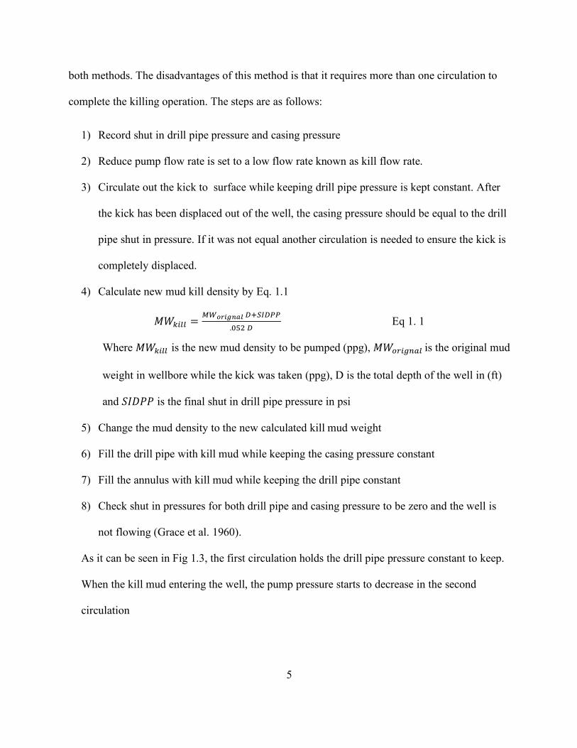
4) Calculate new mud kill density by Eq. 1.1
𝑀𝑊:GMM =+OPQRSTUV WXBYW**
.[\] W Eq 1. 1
Where 𝑀𝑊:GMM is the new mud density to be pumped (ppg), 𝑀𝑊 _G"`9M is the original mud
weight in wellbore while the kick was taken (ppg), D is the total depth of the well in (ft)
and 𝑆𝐼𝐷𝑃𝑃 is the final shut in drill pipe pressure in psi
5) Change the mud density to the new calculated kill mud weight
6) Fill the drill pipe with kill mud while keeping the casing pressure constant
7) Fill the annulus with kill mud while keeping the drill pipe constant
8) Check shut in pressures for both drill pipe and casing pressure to be zero and the well is
not flowing (Grace et al. 1960).
As it can be seen in Fig 1.3, the first circulation holds the drill pipe pressure constant to keep.
When the kill mud entering the well, the pump pressure starts to decrease in the second
circulation

6
Figure 1. 3: Pump pressure changes using the driller’s method
Wait and Weight method
Unlike the drill’s method, the kill mud density is changed and pumped into the well while the
kick is circulated out. This makes it possible for the kick to be circulated out in one circulation
instead to the two needed for driller’s method which is one of the advantages of this method. The
disadvantage of this method is that it requires more calculation from the crew before the start of
the killing operation. The steps recommend is as follows.
1) Recoded the shut in drill pipe pressure and casing pressure.
2) Calculate mud kill density using the same equation as in Eq. 1.1.
3) Calculate initial drill pipe circulation pressure and final drill pipe circulation pressure
using Eq. 1.2 and 1.3
ICP=𝑆𝐼𝐷𝑃𝑃 + 𝑆𝑃𝑃 Eq 1. 2
Pump pressure
Time
Driller's method kill sheet
2nd circulation

7
Where ICP is the initial Circulating pressure in psi, SIDPP is the shut-in Drill pipe
pressure in psi, and SPP is the slow pump pressure in psi which refers to the frictional
pressure loss at a low flow rate
FCP= SPP𝑥 +OeRVV+OPQRSTUV
Eq 1. 3
FCP is the final circulating pressure in psi and MW are the mud weights in ppg for both
kill and original muds.
4) Plan the pumping schedule using a graph of the pump pressure vs volume of mud being
pumped (known as kill sheet) from the start of the kill operation till the kill mud fills up
the drill pipe Fig. 1.4. The pump pressure starts from initial circulating pressure and end
with final circulating pressure when the kill mud fills up the drill pipe. The steps are
decided based on the difference between ICP and FCP divided by the volume of mud
required to fill up the drill pipe.
5) Change the mud density to the new calculated kill mud weight
6) Fill the drill pipe with kill mud while following the pump schedule as in step 4
7) Fill the annulus with kill mud while keeping the drill pipe constant
8) Check shut in pressures for both drill pipe and casing pressure to be zero and the well is
not flowing (Grace et al. 1960).

8
Figure 1. 4: Pump pressure changes using the wait and weight method
1.2.2 Well control with in Managed pressure drilling
Special well control capabilities of MPD systems
The strategy for well control when a kick is taken differs when Managed Pressure Drilling is
being applied. It involves collection of tools to control the backpressure, so it is reactive and
proactive for the kick tolerance in the well. The system is reactive when the well is drilled
conventionally and the RCD tool is existing for added safety on any unexpected downhole
problem. While the system is proactive when it designed during the drilling plan to employ the
MPD technology for more precise wellbore profile pressure (Hannegan and Fisher 2005). The
first reaction to an influx is not necessarily an immediate shut in of the BOP. Some small size
kicks can be handled with only choke pressure applied. When the kick is of a bigger size and
cannot be controlled by the MPD equipment, conventional well control procedures are applied.
The main procedure of managed pressure drilling is to make the circulation system as a closed
loop where the pressure on the annulus is controlled by the MPD choke manifold to keep bottom
Pump pressure
Volume of mud pumped
Wait and Weight's method kill sheet
ICP
FCP

9
hole at the desired pressure. The primary use of constant bottom hole pressure is when the
window between pore pressure and fracture pressure is narrow and an exact value of BHP needs
to be applied and varied depending on the operation.
Dynamic well control
Dynamic well control is defined in this context as continuing mud circulation even if the gas kick
has entered the well without shutting in the well. There are many benefits to this procedure:
1) With continued circulation, frictional pressure added to ECD is still in effect. This
prevents any additional influx from entering the well form loss of pressure exerted on
bottomhole.
2) The ability to rotate the pipe further helps in solving a stuck pipe issue.
3) Quicker overall process for full circulations to get rid of the gas in the wellbore.
4) Less pressure is exerted on the shoe since the surface applied pressure needed is lower do
the frictional pressure loss from circulation (Rajabi, Hannegan, and Moore 2014).
Drilling while circulating influx case history
There are many instances where “flow drilling” was applied successfully. Flow drilling is
continuing drilling without shutting in when the well is flowing and hydrocarbon influxes enter
the well. Both regular rate circulation and pipe rotation are taking place even with a kick in the
wellbore. The influx, whether it was gas or liquid, is separated out in the surface from the mud
(Rajabi, Hannegan, and Moore 2014).
Among these successful examples is an example in the Austin chalk. A drilling challenge was
encountered in a fractured carbonate formation with high pressure and high temperature

10
environment. A combination of UBD and MPD was used to complete the well successfully. The
MPD was used to evaluate the limits of downhole pressure operations which helped in easing the
handling limits of UBD. Underbalanced drilling was utilized by allowing the influx to enter the
well. Drilling is continued until the influx cannot be handled by MPD. When that happens, well
control relays on the traditional BOP shut in. The equivalent mud weight was small as 0.5 ppg
between pore pressure and fracture pressure. The case was successful due to the use of PWD.
PWD has helped in monitoring ECD and allowing continuing drilling while circulating out
influx. The strategy involved taking several kicks. In this case study, repeated well control
situations caused damage to the annular preventer and variable bore rams especially with the
varying properties of mud and the kick fluid plus the high temperature (Elmore, Medley, and
Goodwin 2014).
Micro flux Detection of kicks in OBM
Santos have analyzed real scale data which has also been utilized in this thesis. The main
purpose of the tests was to see the capability of the micro flux system to detect a kick in OBM
which has been known to be difficult due to the solubility of gas in oil. The tests were done in a
11 ppg oil mud with 70% volume diesel. The results showed a positive response detecting kick
in OBM as accurate as WBM. The main rational that was proposed for this was the accuracy of
the flow meter deployed in the choke manifold. It is able to detect kicks as small as 0.5 bbl in
contrast to basic metering systems deployed in rigs with 5 bbl detection volume (Santos et al.
2007). As can be seen in Figure 1.5, a simulation for diffract gas kicks volumes in both WBM as
well as OBM. It shows the expected results of pit gain for OBM was smaller than that of WBM.
Another phenomena that was worth noting here is that at lower gas kick volumes, the pit gain for

11
both mud types were virtually the same. Within the capabilities of micro flux system this
detection can be easily made.
Figure 1. 5: Pit gain comparison for OBM and WBM
Well Control Matrix
The well control matrix is a guide to both the drilling crew and the MPD personnel. It clearly
states at which point the responsibility of the kick mitigation shifts from MPD personnel to the
drilling crew. The MPD system can process small size kicks without interrupting the drilling
process. The threshold for the size of the kick depends on the following factors: rotating control
device rating, formation fracture pressure, gas handling capacity, and liquid handling capacity of
the rig. WCM is to be built and discussed before drilling starts (Rajabi, Hannegan, and Moore
2014).

12
Literature review of simulation studies on initial responses to gas influx during MPD operations
Several theses have been published with regards to well control in MPD operation(Davoudi
2009; J. E. Chirinos 2010; Guner 2009; Piccolo 2013; Das 2007). Specifically, CBHP
application in MPD.
Das
Back in 2008, Das thesis was to simulate different well control initial responses within MPD
constant bottom hole pressure application to evaluate the benefits and the drawbacks of each
response. The simulated initial responses included shutting in the well, increasing back pressure
through choke, increasing flow rate and collectively apply both back pressure and increase in
flow rate. The kick fluid types studied were both gas and oil. The simulation was carried in a
software called Ubitts.
The outcome of Das’s simulation study showed that the best initial response depends on the
availability of certain equipment, geometry of the well, and the main objective while carrying out
well control (reducing maximum casing pressure, keeping weak formation enact, staying within
RCD rating). One sole best initial response was not identified as each initial response had
advantageous and disadvantageous. All simulations were based of a WBM drilling fluid type. In
MPD application, each well is a standalone well that needs to be thoroughly studied to find its
own best initial response in case of well control. In this study, no real scale experiments were
carried out for validation (Das 2007).

13
Davoudi
Davoudi also evaluated nine different initial responses to an MPD well control incidents. He
used same industry well configuration of simulated examples as Das did. However, the software
used was Drillbench (DynfloDrill) which serves as a multiphase transient flow system. The case
simulated was a kick produced by a higher formation pressure than planned. Guner and Das
studied an addition of instability of bottom hole pressure and shallower formation of higher
pressure cases (Davoudi 2009).
The focus of Davoudi’s study was a weak zone above the high-pressure zone that had loss
circulation when traditional well control procedures was applied. The criteria that was used to
detect the presence of a kick is a 2-bbl. gain with accurate flowrate measurement and 20 bbl. for
inaccurate measurement. To validate the data historical real-life experiments carried out in 1986
in LSU #2 was used to compare results of dynflodrill (DFD).
When the data was validated for the use of Dynflodrill, the steady state case showed less than 6%
error for Robertson-stiff rheology model and Dodge_Metzner friction factor model showed the
least error.
The outcome of the evaluation of the nine-different circulating and non-circulating responses
showed that when there is an accurate flow meter, the best response was a rapid increase of
casing pressure, while if flow meter was not accurate an immediate shut in was recommend. As
in the flow chart Fig 1.6 (Davoudi 2009).

14
Figure 1. 6: Best initial response results(Davoudi 2009).
Chirinos
Chirinos thesis has three main methods: 1) Increasing the pump pressure gradually to minimize
BHP irregularities while circulating out any gas influx. 2) Approximating Formation zone
pressure while taking a kick in CBHP operations in MPD 3) Estimating maximum casing
pressure to be planned for in drilling programs by a simple method of triangular gas shape. All if
the three methods utilized both simulation data and real life experiments done in PERTT lab in
1986 for DEA project 7 as well as some experiments done in 2009 by the LSU MPD consortium
(J. E. Chirinos 2010).
In Chirinos work, the full-scale test was done after the gas influx has entered and the process of
circulating out the kick to obtain an approximate Constant BHP. Both Simulations using DFD
and real life experiments showed around the same BHP with no significant fluctuations in
Downhole pressure (J. E. Chirinos 2010). The actual BHP changes that happens during a pump
start up happens due to different factors. One of which is the crew’s ability to respond fast, the
presence of an automated system, and the geometry of the well. The slimmer the well the more
fluctuations there is in the BHP. This is primary caused by the BHP being affected by the size
occupied by the gas with in the annulus weather around DC or regular DP. However, the LSU #2

15
experiments showed a reliable steady BHP within ±25 psi when compared to the acceptable
overbalance.
Maximum Casing Pressure Studies: one of the most important parameters to be estimated before
spudding the well is the maximum casing pressure. This pressure is important to design the
casing type, BOP rating and RCD rating in the case of MPD. Chirinos applied a simple method
using Ohara’s triangular gas distribution was applied. There are few assumptions that are
necessary to be addressed to use this method. Single bubble gas with no slippage or dissolution
is assumed. The method uses real gas law and the frictional pressure is negligible. The main idea
of the Ohara method is to treat the gas as tringle with each vertex having different velocities.
These velocities depend on gas bubble depth and inputting that variable into an empirical
correlation made by Ohara (J. Chirinos, Smith, and Bourgoyne 2011; J. E. Chirinos 2010).
Chirinos focused on the circulating stage of well control during CBHP in MPD. DEA project 7
data were used to validate water based mud (circulating cases) simulations. As can be seen in
Figure 1.7, 4 different formulae were applied to estimate maximum casing pressure. The best
match was the Ohara method with only 25 psi difference than the actual. This shows that, at least
for this LSU #2 geometry, range size of kick , and mud rates ranges, well control maximum
casing is properly estimated by Ohara. However, it is worth noting that this geometry is the same
used by Ohara and that could induce bias in the results (J. E. Chirinos 2010).

16
Figure 1.7: Maximum casing pressure using different formulas (Chirinos 2010)
1.3 Pipe Rotation and Eccentricity Effect on Frictional Pressure Loss
The effect of pipe rotation has been studied and a number of experiments have been conducted to
analyze the effect of the rotation in the pressure losses. Different literature and models estimated
the flow in the annuli using the Yield Power Law(YPL). In 1979 a numerical solution was given
by Hank for laminar flow in concentric annuli. Also, in 1995 inner pipe rotation in both
Newtonian and Non Newtonian fluid was studied by Escudier and Gouldson. In, 2006
Ozbayoglu and Omurla used the Computational Fluid Dynamics (CFD) to understand the
frictional loss in the annuli especially for eccentric drill string. Erge studied the effect both
numerically and experimentally. Yield Power Law (YPL) model was used in his experiment as a
Non-Newtonian fluid. The effect of eccentricity was found to be significant, a decrease of 44%
in the pressure losses for the range of properties of the tests conducted. The effect of the rotation
was investigation in concentric scenarios and found that as the rotation increased, the pressure
loss increased (Erge et al. 2015).

17
Eccentricity has a direct effect on the pressure loss by reducing the annular frictional pressure.
YPL is used because of the existing of three variables that fit most of the drilling fluid. The
problem with the YPL is the complexity of finding the pressure losses, Reynolds number and
velocity profile (Erge, et al., 2015).
1.4 Two Phase Flow in Wellbore with Gas Kick
1.4.1 Initial Back Box Models.
The study of two phase flow in pipes is a complex process. It involves many variables. These
variables consist of the properties of each phase, the flow mechanism and velocity for these
phases, and in addition, the interaction between these two phases. Early studies of two phase
flow needed some major assumptions to conclude a reasonable approximation of the flow.
“Black box” models early studies did not involve the details of flow patterns (Shoham 2005).
Homogenous No-Slip Model
One of the “black box” models treats the system as a single-phase model. It assumes a
homogenous phase that has the average properties of the two phases. This model also averages
the velocity of the two phases. This means that the two phases are undistinguishable. These
approximations assume that there is no slip between the phases (Shoham 2005).
The assumptions of this model are: steady state flow, one average phase that represents the two
phases, no slippage takes place between phases, compressible fluid of each phase, the area of the
cross section may vary and mass could transfer between the two phases. The first few
assumptions provides, especially the no slippage assumption, a limitation to the accuracy and
applicability if the model.

18
Separated Model
The other extreme approach for representing two phase flow is treating each phase separately. In
contrast to the homogenous model, it assumes no interaction between the two phases. The liquid
phase and the gas phase are analyzed separately as a single-phase flow with applying the
hydraulic diameter method. The hydraulic diameter is the equivalent diameter that each phase
occupies in the cross-sectional area of the pipe. Each of these phases is then independently
evaluated and treated for frictional factors and heat transfer for instance (Shoham 2005).
1.4.2 Recent Modeling.
Recent models are more rigorous in representing the two phase flow behavior. The modeling
method could range from experimental to exact solution. It also includes intermediate methods
such as numerical simulation and a combination of the empirical results and a simple physical
model. The two phase studies include many variables such as volumetric flow rate, in-situ liquid
hold up, no slip liquid hold up, superficial velocity, actual velocity, and slip velocity among
many other variables (Shoham 2005) .
In situ liquid hold up (HL) is defined as the “element in two phase flow field occupied by the
liquid phase”. When the system has no slippage which is only accurate in few cases, the no slip
liquid hold up (lL) is equal to the in situ liquid hold up. When there is no slippage in between the
two phases (velocity of liquid is equal to velocity of gas) lL is calculated as the following
equation
𝜆 f =𝑄f
𝑄f + 𝑄"
Where 𝑄f is liquid flow rate, 𝑄" is gas flow rater and 𝜆 f is the in situ liquid hold up.

19
Superficial velocity is defined as the velocity of each phase if only that phase was present in the
pipe such that for liquid superficial velocity 𝑣iM =jkl
where A is the cross sectional areal of the
pipe. The actual velocity however is the velocity of each phase divided by the fraction of the
volume occupied by that phase. The difference between the two velocities is known as the slip
velocity.
To further examine two phase flow compared to single phase flow, a critical difference is studied
which is the two phase flow patterns. The pattern is defined as the geometrical configuration of
each phase on the pipe. The pattern depends on the flow rate of the gas, the geometry of the
system (diameter and angle of inclination) as well as fluid properties of each phase (density,
viscosity and surface tension). Fig 1.8 shows the different patterns that were recently commonly
agreed on by researchers(Shoham 2005).
Figure 1.8: Flow patterns of two phase flow in vertical wells(Shoham 2005).

20
The main two flow patterns that are considered for this research is the slug flow as well as the
dispersed bubble flow. Slug flow: The slug flow represents the flow of large bubble with a bullet
shape known as the “Taylor-bubble”. The bubble occupies most of the cross-sectional area of the
location it is in. This pattern is used in this research with only one bubble of gas coming up the
well in the cases considered and referred to in later chapters as single bubble model. In contrast,
dispersed bubble flow: This flow occurs at high liquid rates. The gas bubbles are small in such a
way that the gas and liquid has the same velocity which supports the no slip homogenous case.
Which was briefly examined for the model of dispersed bubble flow in water based mud
(Shoham 2005).

21
CHAPTER 2: STATEMENT OF PROBLEM AND APPROACH
2.1 Statement of Problem
MPD system of well control allows for circulating out a certain volume of gas using the MPD
choke without the need to revert back to conventional shut-in methods. This reduces
unproductive time within drilling operation. In some cases, the operation being carried can
proceed uninterrupted including drilling. This is made possible, partially, by the use of the
rotating control device (sec 1.1.3) that provide the needed pressure control while allowing for the
drill pipe to be rotated.
The possibility of rotating the drill pipe while the gas is being displaced out of the well raises the
question of the effect of that rotation on integrity of the operation including the RCD required
rating. The maximum anticipated casing pressure can alter by rotation due to two physical
phenomena. First, the introduction of pipe rotation can change the annular frictional pressure loss
calculated for the system. Second, the rotation of the pipe can allow for breakage of the gas
bubble into smaller scattered bubbles throughout the wellbore instead of one single body of gas.
These physical phenomena work differently depending on the mud type, mud properties and
operational variations. For example, in an OBM system, the gas can dissolve in the mud whereas
the solubility of gas in WBM is small. In addition, the gas distribution throughout the well is
expected to behave differently with well inclination, flow rate, mud properties and possibly pipe
rotation. Mud type, mud properties and gas behavior in the wellbore have been taken into
account to evaluate the effect of pipe rotation on the casing pressure while circulating out an
influx on an MPD choke and simultaneously rotating the pipe whether for drilling or any other
related operation.

22
2.2 Approach
2.2.1 Overview
The approach of addressing the problem was carried by, first, analyzing real scale kick
circulation tests. These tests were carried in a controlled environment that mimicked downhole
conditions with a gas influx entering the wellbore. These tests included a variation of mud
properties, mud kill rates and mud types (OBM and WBM). The casing pressure profiles were
gathered from these tests. However, these tests lack the effect of the pipe rotation as
configuration is fixed in the tested well. Second, correlations were applied to estimate the effect
of frictional pressure loss. These changes in frictional pressure loss is caused by pipe rotation and
as a result changes the casing pressure values. These correlations are by Erge (Erge et al. 2014)
and Ozbayoglu and Sorgun (Ozbayoglu and Sorgun 2010). The study was separated into three
different models and cases: dissolved gas in OBM, single bubble in WBM and dispersed bubble
in WBM.
Dissolved gas in OBM
The oil based mud cases were simplified by assuming that all gas was dissolved in the mud and
the correlations were carried with the approximations of liquid only in the wellbore. Although
this assumption is not truthful for all real operational cases, the test procedure for the real scale
experiments were carried in a manner that ensures the dissolution of the gas in the mud prior to
circulating out the influx.

23
Water based mud
Single bubble model
For the case of water based mud, the assumption of gas dissolution in mud is no longer valid.
The volume of gas and its expandability need to be taken into account. The approach to address
WBM cases were first carried by the use of the common, however unrealistic, single bubble
model. This model assumes that the entire volume of gas in the wellbore stays as a single body
of gas and does not break down nor distributes throughout the wellbore. The well was divided
into three different sections for each time step; two liquid regions and one gaseous phase region.
The gas volume at each time step was calculated using the ideal gas law and the location of gas
was evaluated using a correlation of gas velocity from the same real scale data set analyzed in
this work. The model is explained in detail in Chapter 4.
To further investigate the validity of the single bubble model, extensive analysis and review of
the gas bubble breakage and distribution is discussed in Chapter 5.
Dispersed bubble model
The study of the validity of the single bubble model suggested that the gas is more likely to be
distributed throughout the well and the bubble does not stay in one gaseous phase. A study of
the effect of a larger size gas bubble breakage into smaller size bubbles on the maximum
anticipated casing pressure was conducted. This model assumes the other extreme of the
spectrum, compared to the single bubble model. It assumes that the gas bubble is broken down
into very small bubbles either caused by high rotational speed, different operational variations,
and/or well inclination. The assumption entails that these gas bubbles were very small that no

24
slip velocity is present between the two phases and the dispersed bubble pattern equations are
used. Further details are discussed in Chapter 6.
2.3 Real Scale Experiments in LSU#2 Well
In 1986, a consortium of professional companies along with Louisiana State University
personnel conducted real-life scale field analysis of well control. The PERTT lab setup in LSU
allows for a full size well control experiments. In these tests, approximately 10 bbl of gas is
injected into a point close to the bottom of the well. These experiments are the closest s to a real
life kick in an actual well. The test was repeated over 20 times for both WBM systems as well as
OBM systems. When the well was filled with WBM, nitrogen was injected except for few
natural gas cases. For wells with OBM, natural gas was injected in all cases. Different mud
weights, mud rheology, mud rates, gas rates have been tested in combination to result in a
comprehensive study for both mud types. Shown in Table 1.1 is for water based muds and Table
1.2 is for oil based muds (“DEA Project 7” 1986).
2.3.1 Real scale well schematic
The tests were completed in LSU #2 well in the PERTT lab. As Fig 2.1 illustrates, The well is
5884’ deep with 9 5/8’’ casing to bottom. The well has a 3 ½’’ tubing that reaches 5822’ that
was used to circulate the mud. Another 1 1/4’’ pipe is located inside the 3 ½’’ tubing used to
inject gas at the depth of 5852’.
Eccentricity of LSU#2
The eccentricity of the LSU#2 well is not certain. For that reason, multiple scenarios of
eccentricity were studied throughout the analysis of the tests.

25
Figure 2.1: LSU #2 Well Schematic (“PERTT Lab Features” 2017).

26
2.3.2 Mud properties of real scale experiments
Multiple tests with gas injection were conducted. Various mud properties for each test were used.
As in Table 2.1 and Table 2.2, each test number was repeated 4 to 5 times with different kill rates
and mud circulation rates.
Table 2.1: Water based mud properties for each test Test # Mud wt., ppg PV YV 10 sec
gel 10 min gel
1 8.6 7.8 1.8 3.8 3.8 2 8.7 24.2 20.6 21.8 16.6 3 12.4 21.0 4.0 8.8 6.0 4 12.4 28.4 14.0 19.0 12.4
Table 2.2: Oil based mud properties for each test Test # Mud wt., ppg PV YV 10 sec gel 10 min
gel 1 7.92 13.00 3.60 8.60 6.00 2 7.98 20.00 6.40 12.40 6.60 3 12.92 33.60 7.60 20.40 15.80 4 12.80 39.80 16.20 27.80 21.20
2.3.3 Real scale experiments data output
While each test was conducted, the data recorded summarized in Table 2.3.
Table 2.3: Real scale expriment recorded data. Data unit notes Drill pipe surface pressure psi The gauge was placed in the choke manifold.
The pressure needs to be adjusted to friction Surface casing pressure psi Circulated out mud choke in pressure psi Circulated out mud choke out pressure psi Gas wellhead pressure psi Gas wellhead flow rate scf/hr Needs to be used with caution due to flow
meter calibration issues Mud flow rate gpm Mud tanks volume bbls Mud gain/loss Affected by changes in mud flow rate or
leaking valves Mud density in and out ppg using micromotion

27
2.3.4 Test procedures
The gas injecting procedure starts with the correct manifold valve positions. It ensures a flow
from gas storage wells into the 1 ¼’’ gas injection lines into LSU#2. After the initiation of the
gas injection, the PERTT lab staff monitor pit gain. The gas will displace mud in the 1 ¼’’
tubing. When the pit gain reaches 9 to 10 bbl., the injection process stops (“DEA Project 7”
1986).
After 9-10 bbl. of gas has been injected, a pump is turned on to displace the gas volume in the 1
¼’’ pipeline. There are separate manifold lines for each mud type (WBM and OBM). The
Schlumberger gradiometer representative monitors the gas going into the 3 ½’’ -9 5/8’’ annulus.
Once all gas has passed the gradiometer position, the PERTT lab staff turns off the pump (If the
test required the gas to be circulated out after injection. The pump stays on operating position,
mud is only injected between 1 ¼’’ tubing and 3 ½’’ tubing). In all these tests, bottom hole
pressure was kept constant. This is accomplished by applying surface pressure on the 1 1/4’’
tubular. The gradiometer is relocated closer to the surface line. The gradiometer records the
arrival of the gas bubble to its location. OBM test take a different route to determine the gas
being displaced into annulus. The gas goes directly into solution in OBM annulus choke on the
annulus is closed. Once choke pressure on the 1 ¼’’ pipe stabilizes, it the sing that the gas went
into solution.
2.4 Pipe Rotation Frictional Pressure Loss Effect Correlations
The rotation of the pipe effect on pressure drop is to be applied based on the work done by both
(Erge et al. 2015) and (Ozbayoglu and Sorgun 2010). Field measurements using PWD showed an
increase in ECD when RPM is increased (Erge et al. 2015). However, the literature varies on the

28
effect of rotation on the frictional pressure as has been discussed previously. In YPL mud model
when m ≤ 1, the fluid is shear thinning which means the higher the velocity or shear rate, the
lesser the apparent viscosity (slope of shear stress vs shear rate at a certain shear rate). The basic
model is in Eq 2.1.
𝜏 = 𝜏= + 𝐾𝛾F Eq 2. 1
Where 𝛕𝐲 is the yield point shear stress in (Pa) , K is the consistency index of fluid in (Pa.sm) and
m is the flow behavior index (no unit).
When the shear thinning behavior of fluid takes place, higher liquid velocity is expected to result
in a decrease in frictional pressure loss because of the lower apparent viscosity. Nevertheless,
the inertial forces could act against viscous forces and increase the frictional pressure. For that
reason, Erge conducted a study on a 90 ft horizontal pipe with a rotating inner pipe to measure
the annulus pressure loss. The researchers have developed a correlation to best estimate the
frictional pressure loss depending on the flow regime with pipe rotation. The eccentricity of the
drill pipe was also included in the correlation (Erge et al. 2015).
Erge Correlation
The proposed formula first starts with finding the wall shear rate from the rheology model as in
Eq 2.2:
𝑄 = pqr
]∙tu/w∙xyr( F$X]F
)|𝜏p − 𝜏=~u�ww (𝜏p +
F$XF
𝜏=) Eq 2. 2
Where h = �P��R]
and w = �] (D^ + DG), D^ is the outer diameter, DG is the inner diameter of the
annuls in (m). 𝜏p is the shear rate at the wall in (Pa), and Q is the flow rate in (m3/s).

29
Eq 2.2 is applied to the mud specific rheological model. The shear stress is found using mud
specific shear stress vs shear rate graph.
Then the approximation of the generalized flow behavior index is found using (Ahmed and
Miska 2008) equation as in Eq 2.3.:
%�$X]�
= %F$X]F
[1 − � $$XF
�𝑥 − ( F$XF
)𝑥]] Eq 2. 3
Where 𝑥 = x�xy
, N is the generalized flow behavior index. In the mud properties of LSU #2 case,
m was 1 as in Bingham plastic rheological model. Also, generally, whenever 𝑡=is zero, as in the
regular power law, the N would be equal to m.
The Reynolds number is then used for YPL.
𝑅𝑒�*f =$]��r
�y Eq 2. 4
Where 𝜌 is the density of the liquid (or mud) in (Kg/m3) and 𝑣 is velocity of liquid in (m/s)
𝑅𝑒�*f is calculated to check the flow regime. Flow regimes defined in Erge’s work are laminar,
transitional, and turbulent. The criteria for flow regimes is provided in Eq 2.5 and 2.6. If the
𝑅𝑒�*f < 𝑅𝑒$, the flow was laminar. If 𝑅𝑒$ < 𝑅𝑒�*f< 𝑅𝑒], the flow is transitional and if
𝑅𝑒�*f > 𝑅𝑒], the flow was turbulent.
𝑅𝑒$ = 2100 · [𝑁[.%%$(1 + 1.402𝜅 − 0.977𝜅]) − 0.019𝑒𝑁�[.���𝜅] Eq 2.5
𝑅𝑒] = 2900 · 𝑁�[.[%¡)8u¢.£¢¤¥ Eq 2.6
Where 𝜅 = WRWP
, 𝑒(𝑒𝑐𝑐𝑒𝑛𝑡𝑟𝑖𝑐𝑖𝑡𝑦) = ]«WP�WR
, E is the distance of the drill pipe from the center of
the annulus in (m).

30
In most of the cases of the real scale experiments, the flow is laminar. For laminar flow, the
frictional factor is found using Eq 2.7
𝑓M9F,®^` =]¯
)8°±k Eq 2.7
The above equation is for the frictional pressure not accounting for pipe rotation. To add the pipe
rotation factor 𝑓M9F,®^` is multiplied by c (Eq 2.8- Eq 2.11)
c³´µ = 0.2287 · N − 0.0580 · Fº + 0.1237 · wº + 0.4289 Eq 2.8
c¼½´¾¿ = −1.0267 · N − 0.0096 · Fº + 0.0390 · wº + 1.2422 Eq 2.9
Fº =/Á´³ 1õĽſ¿Âþ ÆýÇÅ
ÆýÇÅ ½ÅÈɽź ¼Ã ÊÉÇ˳ŠÄÂÄÅ ¿Â¾É¿Ãºó³Ì Eq 2.10
ωº =Î( QÏÐwRT)
\[[ QÏÐwRT Eq 2.11
N is the generalize flow behavior index found by Eq 2.3, Fd is the dimensionless force defined in
Eq. 2.10 (it was set to zero for LSU #2 data as the drillpipe is in tension) and ωº is the
dimensionless speed of rotation and ω is the rotational speed in RPM. Then to find the frictional
pressure loss (FP) Eq 2.12 used, where f ( frictional factor) is modified using Eq 2..8 or 2.9
𝐹𝑃«_"8 =]ÑÒ�r
�Ó��Ô× 𝐿 Eq 2.12
L is the length of drillpipe that frictional pressure loss was subjected to in (m).
The units from this correlation are metric. Then, units were converted from metric to field units
for parameters of the LSU#2 case and mud properties. The experimental tests that Erge based his
correlation on were done for a range of eccentricities. The range of flow rate is 0-120 gpm and
rotational speed is 0-120 RPM. The mud properties were done on a power law rheological model
that falls around the rheological model of the real scale experiments’ mud (Erge et al. 2015).

31
Ozbayoglu and Sorgun Correlation
To apply this correlation, effective axial viscosity (µμÅ×)and radial viscosity (µμÅØ)are defined as
follows in Eq 2.13 and 2.14
µμÅ× = �Ù(�Ó��Ô)uÚÛ
$¯¯ �uÚÛ� Ü
]X uÛ
[.[][�ݵ
Eq 2.13
µμÅØ = K($µ)µ € �$
à�$�µ
Eq 2.14
€ = |�Ór��Ôr~�Ór
) �$\á�$�µ
(1 − (�Ó�Ô)]/µ)�µ Eq 2.15
DÃ and DÂ are outter and inner diamter of the pipe, respetivly in (ft), K is the consitincy index in
(lbf/100ft2sm), m is the flow behavior index which is dimetionless, 𝑣 is the axial flow velocity in
(ft/s) and ω is the rotational speed of drillpipe in RPM
Then, these viscosities are inserted in a Reynolds number equations for separately defined axial
Reynolds number (Re9) and radial Reynolds number (Re_) ( Eq 2.16 and Eq 2.17, respectively)
and the frictional factor depends on Total Reynolds number(ReE) as follows:
Re9 =ä\äÒ�(�Ó��Ô)
åæ× Eq 2.16
𝑅𝑒_ =].[]\� Î (�Ó��Ô)�Ô
åÏQ Eq 2.17
The frictional pressure factor is then decided on the following constrains and limits,
𝐼𝑓 (ReE) < 3000 𝑓 = 8.274Re9�[.¡[ä\ + 0.00003 𝑅𝑒_ 𝐼𝑓 3000 < (ReE) < 7000 𝑓 = 0.0729Re9�[.%[$ä + 0.00011𝑅𝑒_ 𝐼𝑓 7000 < (ReE) < 10000 𝑓 = 0.006764Re9�[.[]�� + 0.0001𝑅𝑒_ 𝐼𝑓 10000 < (ReE) < 25000 𝑓 = 8.28 Re9�[.ä]\� + 0.00001𝑅𝑒_

32
𝐼𝑓 25000 < (ReE) < 40000 𝑓 = 0.006764Re9�[.]]�] 𝐼𝑓 (ReE) > 40000 𝑓 = 0.03039Re9�[.$\¯] These frictional factors are then inserted into Eq. 2.18 to find the frictional pressure loss of the
entire length of section of concern:
𝐹𝑃ç?è =ÑÒ�r
]$.$(�Ó��Ô)× 𝐿 Eq 2.18
Where L is the length if the section that the flow rate and inner pipe rotation is subjected to in(ft)
and FP is the frictional pressure loss in (psi)
The experimental tests that Ozbayoglu and Sorgun based their correlation on were only done for
an eccentric well. The range of flow rate is 0-150 gpm and rotational speed is 0-120 RPM. The
mud properties were based on a power law rheological model that falls around the rheological
model of the real scale experiments mud (Ozbayoglu and Sorgun 2010).
Sensitivity Analysis of Erge’s Correlation Parameters:
A sensitivity analysis on Erge’s correlation model was conducted. The effect of various
parameters such as pipe rotational speed, mud rheology model, and surface applied force on drill
pipe, generalized flow behavior index, flow rate and eccentricity were studied. The range of
parameters that were studied are within the values of the PERTT lab test data. The outcome of
those results only applies to inputs that are of similar values for those in the test mentioned in the
mud properties summery table (Sec 2.3.2) while applying a Bingham plastic modification where
m=1.
The most important parameter studied here is the speed of pipe rotation. Fig 2.2 shows a general
trend of increase of pressure loss with the increase of pipe rotation speed. The rheology model of

33
the mud plays a slight role in the rate of increase. As it can be seen for lower rheology as in
(WBM1), the increase rate is lower than for that in higher mud rheology (OBM2). More
importantly, the expected concentric non-rotating case frictional pressure loss is actually higher
than that of a rotating case. This behavior is not the most common, however, for the set of flow
rate and mud rheology being tested shows a decrease in frictional pressure loss form non-rotation
to rotation case.
Since the geometry of the wellbore being tested is constant (Do= 8.62’’ & Di=3.5’’), the stability
criteria depends on mud properties. For this case (flow rate = 300 gpm, Concentric Annulus E=0,
fd=0) in Fig 2.2, WBM1 follows the transitional flow criterion (Eq 2.9), whereas OBM2 and
OBM3 are under laminar flow (Eq 2.8). This is evident in the bigger effect that pipe rotation has
in laminar flow since its coefficient in the “c” parameter is larger than that of transitional flow as
illustrated in Equation 2.8 and 2.9. When applying this correlation, the increase in rotational
speed does not play a role in defining the flow regime.
Figure 2. 2: Sensitivity analysis on the change of rotational speed
020406080100120140160180200
0 100 200 300 400 500 600
Frictio
nal Pressre loss, Pa/m
Pipe Rotational Speed , rev/min
Sensitivity Analysis Rotational Speed
WBM1 OBM2 OBM3
Q=300gpm
E=0 Fd=0

34
One of the assumptions to apply Erge’s correlation is that the value of N, generalized behavior
index, must be between 0.15 and 0.4 which are illustrated in Fig 2.3 by the red lines. N is a
parameter that is formulated to combine the effect of flow behavior index (m=1 in Bingham
plastic), shear stress at the wall and yield shear stress at a particular flow rate to account for the
profile change in shear stress profile throughout yield power law flow in pipe (Eq 2.3). An
increase in the value of N shows a steady increase in frictional pressure loss in annulus as in Fig
2.3. This is also the result of flow rate increase as in Fig 2.4. For this case, other parameters were
held constant (ω=0.3, Fd=0, Concentric Annulus e=0)
It is important to note the slope change in the Fig 2.3 and Fig 2.4 for OBM3 and WBM1 are due
to the change in flow regime from Laminar flow to transition flow. The onset transition for
WBM1 and OBM2 are illustrated in Fig 2.4
Figure 2. 3: Sensitivity analysis flow behavior index
N=0.40N=0.10
0
20
40
60
80
100
120
140
0 0.1 0.2 0.3 0.4 0.5 0.6
Frictio
nal Pressre loss, Pa/m
Generalized flow behavior index, N
Sensitivity Analysis of N
WBM1 OBM2 OBM3

35
Effect of Eccentricity
The effect of eccentricity for Erge correlation shows that the higher the eccentricity, the lower
the frictional pressure loss. The velocity of fluid in an eccentric well is lower than a concentric
well because of the spread flow is on the larger area. The main change of varying eccentricity is
Figure 2. 4: Senstivity analysis of Flow Rate
the non-rotation case compared to the rotating case. This dictates whether or not the overall
frictional pressure loss is going to increase or decrease when applying pipe rotation. The
accuracy of this observation is crucial for the baseline measurements of the casing pressure from
the real scale experiments. Fig 2.5 shows the effect of changing eccentricity of on the estimated
frictional pressure loss. As the eccentricity (e) increases, the frictional pressure loss decreases.
OBM3 Onset of Transtion(Re1)
WBM1 Onset of Transtion (Re1)
0
20
40
60
80
100
120
140
0 100 200 300 400 500 600
Frictio
nal Pressre loss, Pa/m
Flow Rate, gpm
Sensitivity Analysis of Flow Rate
WBM1 OBM2 OBM3

36
Figure 2.5: General sensitivity analysis for eccentricity
The frictional pressure loss with rotation is not affected by the eccentricity as can be seen in Fig
2.6. The main effect happens when the drill pipe is not rotating (i.e. ω=0).
Figure 2.6: General sensitivity analysis for eccentricity
10
15
20
25
30
35
40
0.00 0.20 0.40 0.60 0.80 1.00
Frictio
nal Pressre loss, Pa/m
Eccentricity, e
Eccentricity Analysis
10
15
20
25
30
35
0 100 200 300 400 500 600
Frictio
nal Pressre loss, Pa/m
Pipe Rotation Speed, rev/min
Eccentricity Analysis WBM1
e=1 e=0.5 e=0

37
Comparison between the correlations
A comparison between the results of the two correlations for the same mud properties, flow rate,
and well schematic (including only eccentric case limited by Ozbayoglu and Sorgun correlation)
is shown in Fig 2.7 and 2.8. For a flow rate of 90 gpm and the mud properties for WBM1, the
frictional pressure loss for Erge’s model was higher than that for Ozbayoglu and Sorgun
correlation. The increase in speed of rotation in both correlations showed an increase in frictional
pressure loss. Non-rotation case of Erge model showed a higher pressure loss than the case with
rotation.
Figure 2.7: Effect of rotation on frictional pressrue loss using Erge correlation example
0
20
40
60
80
100
120
0 20 40 60 80 100 120 140
Frictio
nal Pressre loss, Pa/m
Pipe Rotation Speed, rev/minWBM1 OBM3 OBM2

38
Figure 2.8: Effect of rotation on frictional pressrue loss using Ozbayoglu correlation example
2.4.1 Gas bubble breakage effect
The single bubble model of well control has been the most commonly used model in the case of
gas influx. It can be described as the worst case scenario in terms of maximizing the casing
pressure when the kick reaches the surface. However, this model is not the most accurate as
many physical variations to the operation and mud properties can break the gas bubble into
multiple smaller bubbles. Kill rate, mud type, mud rheology, choice of time for well shut in and
pipe rotation are among those physical variations that can play a role in breaking the gas bubble.
The gas bubble breakage and distribution is discussed in detail in Chapter 5.
0
20
40
60
80
100
120
0 20 40 60 80 100 120 140
Frictio
nal Pressure Loss, Pa/m
Pipe Rotationa Speed, rev/minWBM1 OBM2 OBM3

39
CHAPTER 3: ANALYSIS OF FRICTIONAL PRESSURE CHANGES ON CASING PRESSURE CAUSED BY PIPE ROTATION IN OIL BASED MUDS USING DISSOLVED GAS MODEL
3.1 Overview
The aim of this study is to calculate the changes in casing pressure caused by the pipe rotation in
OBM while a kick is circulated out of the well. As it has been mentioned earlier, the setup of
MPD systems allow for gas kicks to be circulated out while continuing drilling or other related
operations that involve pipe oration. The main factor that alters the casing pressure, considered
for this section, is the change in annular frictional pressure loss when the pipe is being rotated.
This is accomplished by the analysis of the OBM real scale experiments. These experiments
were then coupled with the pipe rotation correlations (sec 2.4) to calculate the frictional pressure
loss of each test.
Four different tests were analyzed for the effect of pipe rotation on OBM casing pressure
operations while displacing the gas to surface. Each test had a distinct set of operational
variations, mud rheology, and mud weight. The procedure for all these tests is similar. This
process ensures that the gas goes into solution in the oil based mud. Then, the kick is circulated
out of the well. The data for the casing pressure profile, mud flow rates, is collected throughout
the procedure. Then, the effect of frictional pressure changes is applied. That change in casing
pressure is analyzed to see if it has any practical changes for the RCD rating for choice.
The general concept of the model for OBM used in this chapter is that the well, with gas
completely dissolved in mud, only contains liquid. Therefore, the correlations of pipe rotation
were applied with assuming only liquid flow in the annulus. This assumption is valid in certain
cases. The study of a gas kick in OBM is significantly affected by the gas solubility in the mud.,

40
especially when the process takes place in a high pressure environment such as downhole
wellbore conditions. A brief study of that effect on the validity of the liquid approximation
model to estimate the frictional pressure loss is included in this chapter.
3.2 Dissolved Gas Model for Oil Based Muds
This model is a simplified model to address frictional pressure changes in OBM systems with
gas kicks. The gas was assumed to be completely dissolved in the mud at bottom hole pressure.
Therefore, when applying the pipe rotation approximation, only liquid is assumed to be in the
wellbore. This assumption is supported by the procedure that was carried for the real scale tests
in oil based mud. The procedure ensures that gas goes into solution before starting the kick
circulation out process as illustrated in Fig 3.1. After approximately 10 bbl. of gas is injected into
the wellbore (step 1), the pump is turned off and the annulus choke is closed to maintain enough
pressure to dissolve the gas into the mud (step 2). When the pressure of the 1 ¼’’ drill pipe
stabilizes (refer to 2.3.1), the gas was decided to be completely in solution. Once this was
established, the circulating out process starts (step 3). The casing pressure changes is
approximated using Eq. 3.1
C𝑃)*+ = C𝑃i�9�G® – FP Eq 3. 1
Where C𝑃)*+ is the casing pressure with rotation, C𝑃i�9�G® is the casing pressure for non-
rotational case ( real scale test data) and FP is the frictional pressure increase calculated from
each correlation ( Erge and Ozbayoglu )using only liquid flow in the well bore. The units are all
in (psi).

41
Figure 3. 1: OBM real scale procedure illustration
3.3 Example of Full-Scale Data Output (OBM)
An example of one of the OBM tests of the real scale experiments data output and measurements
are shown in Fig 3.2. The casing pressure data with time was the main curve that analysis was
run on. Measurements such as the flow rate and mud properties (rheology and density) were
included in the calculation of the frictional pressure loss caused by pipe rotation.
Fig 3.2 also illustrates some of the procedure steps. The kill rate for this test was 90 gpm.
Around min 50, after the gas was injected, the pump was turned off and the annulus choke was
closed to dissolve the 10 bbl of gas is in the mud. At this point, the volume of the mud pit did not
go back to its original value; this is mainly caused by the volume of the dissolved gas added to

42
the circulation system. Once this gas dissolution was established, circulation was restarted
around 110 min mark.
Figure 3. 2: Test 2-5 (OM10) data measurment and output.
3.4 Pipe Rotation Effect on Casing Pressure in OBM Using Dissolved Gas Model
Four different tests were analyzed for the effect of frictional pressure loss variations caused by
pipe rotation on the casing pressure. The frictional pressure loss was calculated for both
concentric and eccentric schematics in LSU #2. Both setups were calculated because the
eccentricity of LSU #2 is not certain. The main outcome of all these test showed an increase in
the casing pressure. The reason is that the frictional pressure loss actually decreases from the
non-rotational case (eccentric and concentric) to the rotational case at 120 RPM. The frictional
pressure loss when the pipe is not rotating has higher frictional pressure loss than when the pipe
is rotating. Practically in the field, this rarely occurs but some experimental results do suggest
60
70
80
90
100
110
120
130
140
0
50
100
150
200
250
300
350
400
0 20 40 60 80 100 120 140 160 180 200 220 240 260 280 300
MUD
PIT VOLU
ME, BBL
PRESSU
RE, PSI AND
FLO
W RAT
E, GPM
TIME, MINCasing Pressure, psi Pump flow rate, gpm Mud Volume, bbl
Q circulation= 133 gpm
Q kill= 90 gpm

43
that the non-rotational case can have a higher frictional pressure loss as in the work of Erge and
the correlation based on it (Erge et al. 2015).
Since OM6 and OM10 tests have the same mud properties and similar flow rates, the effect of
pipe rotation has shown the same trend of an increase casing pressure. The maximum increase of
casing pressure of the OM6 and OM10 tests was a value of 16 psi. This accounts for a 5 %
increase of the average casing pressure of 300 psi and an increase of 4% of the average of 325
psi for Test 2-1 (OM6) and (Test 2-5) OM10 respectively as can be observed in Fig 3.3 and Fig
3.4. This is an increase that probably would not make a practical difference for a case similar to
the LSU#2 data with low mud rheology and only 6000 ft depth.
Figure 3. 3: Effect of pipe rotation using Erge's model for OM6
In Fig 3.5, a comparison between Erge and Ozbayoglu correlations was conducted. The
Ozbayoglu correlation has the starting position before rotation set to be eccentric. The rotation
for the set of data in DEA project mud properties and flow rates has no practical effect. With
150
170
190
210
230
250
270
290
310
330
350
100 120 140 160 180 200 220 240 260 280
Pressure,psi
Time, min
Casing Pressure Diffrence for OM6
Mud out, psi Mud out, psi (120 RPM, Concentric) Mud out, psi (120 RPM, Eccentric)
BHP= 2692 psi

44
only 1 psi decrease, this could be a correlation error. Ozbayoglu correlation was not run on the
rest of the tests because of that small effect.
Figure 3.4: Effect of pipe rotation using Erge's mdoel for OM10
Figure 3. 5: Comparison between Erge and Ozbayoglu eccentric starting position
150
200
250
300
350
400
80 100 120 140 160 180 200 220 240 260 280 300
Pressure,psi
Time, min
Casing Pressure Diffrence for OM10
Mud out, psi Mud out, psi (120 RPM, concentric) Mud out, psi (120 RPM, Eccentric)
150
170
190
210
230
250
270
290
310
330
350
0 20 40 60 80 100 120 140 160 180 200 220 240 260 280 300
Pressure,psi or M
ud pit volume, bbl
Time, min
Casing Pressure Diffrence for OM6
Mud out, psi Mud out, psi (120 RPM) Ozbayoglu Mud out, psi (120RPM) Erge

45
Figure 3. 6: Effect of pipe rotation using Erge's mdoel for OM11
As for Test 3-1 (OM11) as in Fig 3.6, the maximum change of the casing pressure is an increase
of 21 psi for the case of the pipe rotation is 120 RPM assuming a starting concentric layout of
the LSU#2 schematic. The 21 psi difference accounts for 6% increase of the casing pressure and
these results are very similar to both OM6 and OM10 tests with an increase of the casing
pressure instead of the expected decrease.
In Fig 3.7, Test 3-5 ( OM 15) is shown. The effect of pipe rotation on OM15 has the same results
as for OM11. The main difference between the two tests are in the circulation rate while the kick
is being injected. In OM11, the gas is injected with no mud circulation where OM15 had a
circulation rate of 90 gpm while the gas kick was being injected. The overall casing pressure of
OM 15 was higher than OM 11. The overall pipe rotation effect was a maximum increase of 21
psi which is 6% increase in casing pressure.
0
50
100
150
200
250
300
350
400
80 100 120 140 160 180 200 220 240 260 280 300 320 340 360 380
Pressure,psi
Time, min
Casing Pressure Diffrence for OM11
Mud out, psi Mud out, psi (120 RPM, Concentic) Mud out, psi ( 120 RPM, Eccentric)

46
Figure 3.7: Effect of pipe rotation using Erge's mdoel for OM15
3.4.1 RCD rating
The selection of RDC rating is decided based on the maximum anticipated casing pressure. The
above four tests were analyzed to see if any changes of the casing pressure would have a
practical significance on the rating selection of RDC. For all these tests, the changes of the
casing pressure ranged from 4% to 6%. These changes are not significant to recommend a rating
change in the RDC of choice. However, MPD engineers are encouraged to make case specific
calculations of each well to accurately decide the changes on the annular frictional pressure
caused by the pipe rotation because in an environment with such narrow pore pressure and
fracture pressure limits, any change in the frictional pressure loss can help the precision on the
downhole pressure profile.
0
100
200
300
400
500
600
0 20 40 60 80 100 120 140 160 180 200 220 240 260 280 300 320 340
Pressure,psi
Time, min
Casing Pressure Diffrence for OM15
Mud out, psi Mud out, psi (120 RPM, Concentic) Mud out, psi ( 120 RPM, Eccentric)

47
3.5 Validity of the Dissolved Gas Model in OBM
The OBM model in this chapter assumes that the gas is completely dissolved in the wellbore at
all depths. This assumption needs further investigation for the considered tests because gas could
come out of solution at shallower depth and lower pressures. Real scale data for mud flow rate
out of the well shows some variations compared to mud pump flow rate. Each test was briefly
analyzed for this behavior.
Early conclusions made by the team that ran the real scale OBM experiments suggests that the
gas does not come out of solution until after it has passed the choke coming out of the well
(“DEA Project 7” 1986). However, the four tests, except for some poorly recoded data in Test 2-
5, showed an increase in the mud flow rate coming out of the well compared to the pump flow
rate. This increase could correspond to the gas coming out of solution closer to surface. Test 2-1
showed only a brief increase for few minutes. While Test 3-1 (OM 11) and Test 3-5(OM15)
exhibited an increase for a longer period of time. Fig 3.8 shows test 3-1. The flow rate out of the
casing was at an average of 220 gpm where the pump rate was at 90 gpm, that increase continued
for over 100 minutes. The increase of flow rate out of the well indicates some gas coming out of
solution. However, the mass micromotion measurements are not reliable. The micromotion does
not accurately measure the flow rate and the value could be exaggerated. The velocity estimation
of gas dissolved in oil based mud further explained in chapter 4 ( section 4.2.1) shows that the
depth location is shallow when gas comes out of solution (270 ft for some cases) and that the
change in frictional pressure caused by it is negligible.

48
Figure 3. 8: Test 3-5 (OM15) pump flow rate compared to mud flow rate out of well
3.6 Summary of the Results and Conclusion of Dissolved Gas Model for OBM
Analyzing the results from test group of the mud properties of OBM has shown that, the casing
pressure increases with 120 RPM of pipe rotation with a range of 4- 6% increase. Summary of
the results is in Table 3.1. This is primarily caused by the decrease in frictional pressure loss
when pipe rotation is carried. Usually, and based on field data, the frictional pressure loss
increases when the pipe rotates, however, in some experimental data that Erge based his
correlation on, the frictional pressure loss for non-rotational case is actually higher than the
rotational case (Erge et al. 2015). The four tests analyzed in this chapter fall in the range that
exhibits a decrease in frictional pressure loss with rotation.
0
50
100
150
200
250
0 20 40 60 80 100 120 140 160 180 200 220 240 260 280 300 320 340 360
FLOW RAT
E, GPM
TIME, MINPump flow rate, gpm Mud flow out, gpm

49
Table 3.1: Summary of results for OBM test data Test # µp, eq cp/ Pa.s τy, Pa/ lbf/100 ft2 MW,
ppg 120 RPM effect on casing pressure
RCD rating
2-1 (OM6)
.02/20 2.3/6 8 5% increase No change
2-5 (OM10)
.02/20 2.3/6 8 4 % increase No change
3-1 (OM11)
.031/33 3.1/10 13 6 % increase No change
3-5 (OM15)
.031/10 3.1/10 13
6 % increase No change
For practical considerations, the change in casing pressure is insignificant to select a different
RCD rating. Furthermore, for mud rheology and flow rates similar to the real scale tests, it is not
recommended to apply pipe rotation because the rotation increases the planned casing pressure
based on applying the dissolved bubble model as in this chapter. However, precisely controlling
the annular pressure profile and accounting for the rotational frictional pressure changes, is going
to ascertain the downhole pressure limits with narrow pore-fracture pressure operational window.
Further analysis of the flow rate data shows that gas comes out of solution closer to the surface
caused by the decrease in hydrostatic pressure.

50
CHAPTER 4: ANALYSIS OF FRICTIONAL PRESSURE CHANGES ON CASING PRESSURE CAUSED BY PIPE ROTATION IN WATER BASED MUDS USING SINGLE BUBBLE MODEL
4.1 Overview
The aim of this study is to calculate the changes in casing pressure caused by the pipe rotation in
WBM while a kick is circulated out of the well. As it has been mentioned earlier, the setup of
MPD systems allow for gas kicks to be circulated out while continuing drilling or other related
operations that involve pipe oration. The main factor that alters the casing pressure, considered
for this section, is the change in annular frictional pressure loss when the pipe is being rotated.
This is accomplished by the analysis of the WBM real scale experiments. These experiments
were then coupled with the pipe rotation correlations (sec 2.4) to calculate the frictional pressure
loss of each test.
Three different tests were analyzed for the effect of pipe rotation on WBM casing pressure
operations when displacing the gas to surface. Each test had a distinct set of operational
variations, mud rheology, and mud weight. The data for the casing pressure profile, mud flow
rates, is collected throughout the procedure. Then, the effect of frictional pressure changes is
applied. That change in casing pressure is analyzed to understand if it has any practical effect for
the RCD rating selection.
The single bubble model in WBM used in this chapter is a simplified model. It assumes that the
gas kick is going to migrate keeping one single body of gas throughout the circulation process.
The volume of the gas bubble changes as it raises up the wellbore with the change in hydrostatic
pressure is considered using ideal gas law. The closest pattern to this model in two phase flow is
what is known as slug flow (section 1.4.2). The location of the gas at each time step is estimated

51
from correlations from the real scale data being used. The single bubble model, although very
common in the industry, is inaccurate. The gas bubble rarely stays in one single body. A
discussion of the single bubble model validity is included in chapter 5.
4.2 Single Bubble Model for Water Based Muds
Dealing with WBM represents a different engineering question than OBM. The gas kick that
comes from the wellbore no longer dissolves into the mud. The natural gas hydrocarbon stays in
its gaseous phase. This poses further implication about the estimation of frictional pressure loss
caused by pipe rotation. The proposed simple model assumes the kick to be one single bubble of
a gaseous phase. The bubble enters the well and moves up and stays intact as one body of
gaseous fluid. Therefore, the well is divided into three different sections at each time step. 1)
Liquid phase: the section of drilling mud that lies below the gas bubble with the same flow rate
as the pump (i.e. kill rate). 2) Gas phase: the gas bubble itself whose volume is calculated using
the ideal gas law. 3) Liquid phase of higher flow rate: the section of the mud that lies above the
gas bubble and its flow rate is affected by the expandability of the gas below it, resulting in a
higher flow rate than the kill rate. Fig 4.1 shows schematic of the model at one-time step. This
simplification rules out dealing with complex multiphase flow within the well and starts with the
simplest approach.
4.2.1 Location and velocity of gas
For the single bubble approximation, the method used to estimate the velocity and location of the
gas in the well at each time step uses the results from the DEA project 7 correlations. The
correlations includes the rheology and density of mud to normalize the value of velocity as in Eq

52
4.1. It also depends on the average void fraction of gas (𝜷); gas void fraction is defined as the
fraction of the cross sectional area of the
Figure 4. 1: Single bubble model approximation schnamtic at one time step
wellbore occupied by the gas when gas is at a certain point. The average value was taken for gas
void fraction form gradiometer measurements in LSU#2. A correlation that was found by the
DEA project results to estimate the increase in gas velocity compared to liquid velocity is in
Eq.4.1. The extra gas velocity (𝑣Å) is defined as the difference between the gas velocity and the
peak velocity of liquid that occurs in the center of the flow between the two annulus walls. The
peak velocity of liquid is estimated from the OBM tests with the gas dissolved in it taken from
Fig. 4.2 which is a reproduced graph from DEA data analysis. The average velocity is the pump-
induced velocity of mud. The additional gas velocity is then added to that peak velocity to find
the middle location of gas in the well.

53
𝑣Å = (x�Ù£).$](ÒÛ�Òì
ÒÛ).]\ (4.92β + 1.25) Eq 4. 1
Figure 4. 2: Estimate of the peak velocity of mud from the OBM tests [reproduced gragh from
(“DEA Project 7” 1986)]
The ideal gas law was used to find the volume of the gas at a certain point as in Eq. 4.2 where the
volume (Vb) of the kick at bottom hole pressure is known
𝐵𝐻𝑃 𝑉è = 𝑃�𝑉� Eq 4. 2
𝐷" = (𝑡[ − 𝑡) ∗ (𝑣789: + 𝑣8) +fS]
Eq 4. 3
𝐷" is the location of gas depth in (ft), BHP is the bottom hole pressure in (psi), V is the volume
at bottom or at a certain point of time in bbl, 𝑡[ is the time at which the gas has reached the
surface in (seconds), 𝑣 is the velocity in (ft/s), and Lg is the length of the gas bubble in (ft)
The flow rate of section 3 was estimated using Eq.4.4, the mass flow provided from the data
(taken by micromotion before the choke) divided by the density of the mud
𝑄"7F = jVòó/wRT
+O Eq 4. 4

54
4.2.2 Estimation of Frictional Pressure Loss Caused by Pipe Rotation
At each time step, the difference in frictional pressure loss caused by the rotation of the pipe is
applied for the three different sections depending of the length of each section at each time step
as in Eq 4.5. It can also be explained as the weighted average of frictional pressure loss for the
entire well.
𝐹𝑃 = fuEW 𝐹𝑃$ +
fSEW 𝐹𝑃" +
f£EW 𝐹𝑃% Eq 4. 5
Where L1, Lg and L3 are the lengths of section 1, section2 or gas bubble, and section 3,
respectively in (ft) at one point of time as shown in Fig 4.1. TD is the total depth of the well in
(ft). FP is the frictional pressure loss at each section in (psi), FPg is negligible because the
frictional pressure loss for the gas section is less than 10-3psi
Then, that difference is subtracted from the static no rotation casing pressure collected from the
real scale expriments (Eq.4.6)
𝐶𝑃)*+ = 𝐶𝑃i�9�G® – 𝐹𝑃 Eq 4. 6
CP is casing pressure in (psi) for rotating and non-rotating cases. FP is the annular frictional
pressure in (psi) from the correlations as in section 2.4
4.3 Example of Full Scale Data Output (WBM)
One example of the output of WBM test is shown in Fig 4.3. For this test, there is no circulation
while the gas injection was taking place and 90 gpm is used as a kill rate (refer to driller’s
method). For instance, this test’s flow rate for section 1 is 90 gpm. The increased flow rate
Section 3 is 220 gpm. The point of time at which the gas reached the surface (𝑡[) is the point of
increase in mud pit volume.

55
Figure 4. 3: WN2 (test 1-2) data output
4.4 Pipe Rotation Effect on Casing Pressure in WBM Using Single Bubble Model
The main effect on casing pressure while applying the single bubble model is the change in
frictional pressure loss throughout the annulus. When the drill pipe rotates at 120 rpm speed, for
example, the annulus frictional pressure loss is going to differ from a non-rotation case. This
difference is the proposed change on the casing pressure. Since LSU #2 schematic is uncertain,
both eccentric and concentric schematics are applied to find the frictional pressure loss of the
non-rotational case.
Test 1-2: Fig 4.4 shows the results of applying the above-mentioned model to calculate the
casing pressure with rotation. Both concentric and eccentric non-rotational cases use Erge’s
model on Test 1-2 ( Table 4.1). The results showed primarily an increase in the casing pressure
instead of the expected decrease. The overall frictional pressure loss actually was lower with
rotation (120 RPM) than the non-rotation cases. For this case, the maximum increase happens
110
130
150
170
190
210
230
250
0
100
200
300
400
500
600
700
0 20 40 60 80 100 120 140 160 180
Mud
Volum
e, bbl
Pressure, psi, and
flow
rate, gpm
Time
Test 1-‐2
Casing Pressure Mud out,gpm Mud flow rate, gpm Mud Volume, bbl
Q circulation= 0 gpm
Q kill= 90 gpm

56
when the configuration was assumed to be concentric and the pipe rotation is 120 RPM. The
value of the increase was 12 psi which accounts for 2% increase in the overall casing pressure.
Figure 4. 4: Comparison between eccentric and concentric schematic assumptions (Erg’s
correlation)
The eccentric non-rotational cases have a lower frictional pressure loss in the annulus than the
concentric case. The difference between eccentric non-rotational and 120 RPM rotation was
negligible (< 2 psi) using Erge correlations as shown in Fig 4.4 and 4.5. Ozaboyglu correlation,
on the other hand showed a decrease in the casing pressure with a maximum decrease of 16 psi
which is around 3% of the overall casing pressure (Fig 4.5).
Test 1-5: frictional pressure loss was found using Erge’s model by applying the single bubble
model explained earlier. The mud circulation rate while the gas is being injected for this test is
133 gpm, compared to the previous analyzed test of zero circulation rate. The kill rate is 90 gpm
430
450
470
490
510
530
550
570
590
610
630
10:33 11:02 11:31 12:00 12:28 12:57 13:26 13:55
Pressure, psi
Time
Casing Pressure change with rotation for Test 1-‐2
Base 120 RPM Erge concentric 120 RPM Erge Eccentric

57
Figure 4. 5: Comparison between Ozaboyglu and Erge's eccentric schematic
Table 4. 1: Pressures loss for various flow rates and rotational speeds for WBM1 Model Erge Concentric FP, psi Erge Eccentric FP, psi Ozaboyglu FP, psi
Q, gpm à
ω, RPM 90 133 340 90 133 340 90 133 340
0 29 32 12 18 19 29 2 3 13
120 15 17 9 15 17 39 5 11 69
(Section 1), similar to test 1-2. The flow rate out of the well was calculated to be around 340
gpm (Section 3). The frictional pressure loss for non -rotational cases (eccentric and concentric)
was found as well as the frictional pressure loss at 120 RPM. As it can be seen in Table 4.1. at
340 gpm, the eccentric cases (applying both correlations) showed an increase, although
430
450
470
490
510
530
550
570
590
610
630
10:33 11:02 11:31 12:00 12:28 12:57 13:26 13:55
Pressure, psi
time
Casing Pressure with RPM For Test 1-‐2
Base 120 RPM Ozbayoglu & Sorgunn RCD rating 120 RPM Erge Eccentric

58
insignificant, in frictional pressure loss with pipe rotation. This corresponded to a decrease in
casing pressure. However, frictional pressure loss for a 90 gpm static concentric case was higher
than the 120 RPM rotational case. This corresponded to an increase in casing pressure. For that
reason, concentric cases in Fig 4.6 mostly shows an increase for casing pressure. The maximum
increase in the casing pressure is for concentric and 120 RPM with 15 psi that accounts for 3%
increase. However, eccentric cases show a decrease in casing pressure as shown Fig 4.7. The
maximum decrease happens when Section 3 (at 340 gpm) is longer than the other two sections.
The frictional pressure loss when applying Ozbayoglu change is 6% of the maximum casing
pressure with a value of 32 psi as in Fig 4.7.
Test 4-2: The analysis for higher rheology mud as in Test 4-2 (Table 1.1) has been done
discretely accounting for only the maximum casing pressure instead of applying the whole
pressure time profile with time. The frictional pressure changes were taken based on the highest
change scenario (using the highest flow rate: 320 gpm) over the entire well. The maximum
casing pressure for test 4-2 was 640 psi and the maximum frictional pressure effect was a
decrease from concentric non rotational case to a 120 RPM speed of pipe with 34 psi which
corresponded to 5 % increase in the casing pressure. The maximum change on the opposite
direction happens using Ozbayoglu correlation which resulted in an increase in frictional
pressure loss of 12 psi which corresponds to 2% decrease in casing pressure.
In all of the above mentioned cases, the change is not significant enough to cause a change in the
RCD design. The next lower RCD dynamic rating is not reached with pressures changes for due
to the frictional pressure loss caused by that rotation. However, the slightest change in the
frictional pressure loss in the annulus and specially above the casing shoes is important as MPD

59
operations typically addresses narrow fracture-pore pressure window. Even minor changes in the
frictional pressure loss can affect the wellbore stability.
Figure 4. 6: Comparison between eccentric and concentric schematic with Erg’s Model
Figure 4. 7: Comparison between Ozaboyglu and Erge's eccentric Schematic
450
470
490
510
530
550
570
10:33 11:02 11:31 12:00 12:28 12:57
Pressure, psi
Time
Casing Pressure with RPM For Test 1-‐5
Base 120 RPM Erge concentric 120 RPM Erge Eccentric
400
420
440
460
480
500
520
540
560
10:33 11:02 11:31 12:00 12:28 12:57
Pressure, psi
time
Casing Pressure with RPM For Test 1-‐5
Base 120 RPM Ozbayoglu & Sorgun 120 RPM Erge Eccentric
Q circulation= 133 gpm
Q kill= 90 gpm

60
4.5 Summary of the Results and Conclusion of Single Bubble Model for WBM
Three full scale WBM tests measurements and data were analyzed for the effect of pipe rotation
on the casing pressure, and specifically the effect of change in frictional pressure loss on the
casing pressure. A summary of the analysis is shown in Table 4.2. The maximum increase of
casing pressure using the single bubble model is observed when assuming a concentric schematic
and applying 120 RPM rotation for drill pipe. The maximum decrease in casing pressure is
observed when Ozaboyglu is applied for eccentric schematic and a rotational speed of 120 RPM.
For geometries and mud rheology’s similar to DEA project (Shallow wells and low mud
rheology’s), the effect of pipe rotation assuming a single bubble of gas is insignificant with a
maximum of 6% percentage decrease in the casing pressure.
Table 4. 2:Summary of results for single bubble model Test # µp,
eq
cp
τy,
lbf/100ft2
MW,
ppg
𝚫𝐂𝐏
Eccentric &120
RPM
𝚫𝐂𝐏
Concentric&120
RPM
RCD
rating
1-2((WN2) 8
2 8.5 3% decrease 2% increase No change
1-5 (WN6) 7 3 8.5 6 % decrease 3 % increase No change
4-2 (WN20) 33 10 13 2% decrease 5% increase No change
The RCD dynamic rating selection is not changed based on the changes of the maximum casing
pressure when using the single bubble models in rheology’s and flow velocity similar to DEA
project. Furthermore, pipe rotation for the cases discussed does not necessarily aid to the
decrease in casing pressure. The decision to continue with operation that includes pipe rotation is

61
not significantly affected when accounting for only frictional pressure loss changes on casing
pressure. However, in deep offshore cases with tight fracture-pore pressure limits, the effect of
the change in frictional pressure loss is magnified. The accurate estimation of the change in
frictional pressure loss with rotation can further the precision of the downhole pressure profile
values and possibly increase the kick tolerance.

62
CHAPTER 5: VALIDITY OF SINGLE BUBBLE MODEL AND GAS DISTRIBUTION
5.1 Overview
The single bubble model, although used in most well control methods calculations, is believed to
be inaccurate. The bubble is more likely to break into smaller bubbles and distribute throughout
the well as it migrates upwards. The purpose of this chapter is to address the factors that aid or
hinder gas distribution; this is divided into two sections. First, we analyze the gas distribution of
the full scale tests with different operational variations and cross validating the results with the
published literature. Second, we review the effect of pipe rotation on fluid flow through the
discussion of a fluid flow phenomenon known as Taylor vortices. These vortices are speculated
to increase the gas distribution and breaking the gas into smaller bubble.
The LSU #2 real scale experiments results and literature were cross validated with (Rommetveit
and Olsen 1989; Spoerker, Gruber, and Brandstaetter 2012) in regards to factors affecting gas
distribution. The gas distribution (i.e. higher gas breakage effect) has been shown to increase
with the following factors: 1) less well inclination 2) lower mud rheology 3) lower kill rates
Furthermore, a phenomenon known as Taylor vortices which takes place above a certain critical
speed of rotation was proposed to aid to the gas mixing and breakage of the bubble. The Taylor
vortices occurrence has been established for the case of liquid flow in-between two pipes with
the inner pipe rotating(Taylor 1923). Although the gas mixing has not been experimentally
researched for a non-Newtonian fluid with cases similar to a gas kick in the wellbore, evidence
from literature supports the hypothesis of Taylor vortices aiding the mixing of gas in the

63
wellbore and furthering the breakage of the gas (Spoerker, Gruber, and Brandstaetter 2012;
Lockett, Richardson, and Worraker 1993).
It is vital to discuss the gas distribution because the distribution of gas and maximum casing
pressure are closely related. Fig 5.1 shows the correlation between surface gas void fraction and
maximum casing pressure from the DEA project data. The surface gas void fraction is defined as
the fraction of the wellbore occupied by the gas when gas reaches the surface. Lower void
fraction infers higher bubble breakage and higher gas distribution. As can be seen in the figure,
the gas surface void fraction is highly correlated with maximum casing pressure. The void
fraction is dependent on several factors including flow rate, mud properties and type.
Figure 5.1: Correlation between surface gas void fraction and Maximum Casing Pressure
5.2 Gas Kick Distribution in Wellbore
5.2.1 Well inclination effect on gas distribution
A team of researchers from the university of Leoben, performed a simulation using the VOF
(Volume of fluid) multiphase modeling method. The simulation only models 10 meters of the
0
0.1
0.2
0.3
0.4
0.5
0.6
0.7
0.8
0.9
1
0
100
200
300
400
500
600
700
800
900
0 2 4 6 8 10 12 14 16
Surface Ga
s Void Fractio
n
Maxim
um Casing Pressure, psi
Test #Maximum Casing Pressure, psi Surface Void Fraction
Low Rheology

64
well because the depth to annulus width is too high to graphically represent the behavior. Unlike
most well control models of proposing a single bubble of gas moving upward, the vertical well
model clearly illustrates that there is a streaking behavior of that gas and only a portion of gas
stays as a single elongated bubble as in Fig 5.2 (Spoerker and Tuschl 2010). This streaking
behavior is of an agreement with the results of the DEA tests because the results report a
different gas void fraction at the bottom than at the top. When the inclination of the well was
slightly altered, the behavior of the gas took a slightly different pattern. The inclination has
induced a more consolidated bubble towards the upper facing side of the annulus (Fig 5.3). As
the inclination increases, the gas has a tendency to stay in one bubble.
Figure 5.2: Gas bubble flow in mud in vertical open hole over 3 min(Spoerker and Tuschl 2010).
Figure 5. 3: Gas behavior with 1° inclination (left) and 10° inclination (Right) over 3 min
(Spoerker and Tuschl 2010).

65
5.2.2 Mud flow rate effect on gas distribution
Experiments of gas distribution coming out of a full size well found in the literature indicate that
the lower the rate of the kill operation for water based mud, the more dispersed the gas is
(Rommetveit and Olsen 1989). Similarly, DEA project data analysis of the void fraction of gas at
surface showed that the lower the kill rate, the more distributed the gas is in the wellbore. The
data illustrates that gas distribution at surface increases as the kill flow rate increases as in Fig
5.4. For each set of tests, mud properties, kick size, and circulation rates are the same.
Figure 5.4: Effect of kill rate on gas distrbution (“DEA Project 7” 1986).
5.2.3 Mud viscosity effect on gas distribution
Using the DEA project data, for the similar gas distributions at the bottom and same circulation
rate, the increased mud viscosity induces a higher gas concentration at the surface. Fig 5.5 shows
the difference of gas void fraction at surface with all other parameters kept the same except mud
rheology. The higher the rheology, the higher the gas void fraction and, hence, the lower the
distribution of gas. The low mud rheology in the figure refer to a range of plastic viscosity (µp)
0
20
40
60
80
100
120
140
0
0.05
0.1
0.15
0.2
0.25
0.3
0.35
2-‐1 2-‐2 2-‐4 3-‐1 3-‐2 4-‐1 4-‐2Flow
rate, gpm
Surfaace void fractio
n
Test
Gas Void FractionFlow rate

66
of 7-19 eq cp and a yield stress (τy) of 2-4 ³ÊÑ$[[Ѽr
,whereas the high mud rheology refer to a range
of plastic viscosity (µp) of 25-33 eq cp and a yield stress (τy) of 12-9 ³ÊÑ$[[Ѽr
.
Figure 5.5: Mud rehology effect on gas disrubution
Based on the above mentioned factors, optimum combination of the increased gas distribution
and lower casing pressure therefore is low kill rate, low mud rheology and vertical well
orientation. However, the only parameter that can be controlled at the time of the operation is the
kill rate.
5.3 Pipe Rotation Effect on Gas Distribution
In this section, a fluid flow phenomenon known as Taylor vortices is proposed and is speculated
to aid in the gas mixing. When these vortices occur, the gas bubble is suggested to break into
smaller bubbles that is more likely to compromise the single bubble model.
0
0.05
0.1
0.15
0.2
0.25
0.3
0.35
Surface Ga
s Void Fractio
n Low rheology
High rheology

67
5.3.1 Introduction to Taylor Vortices
In 1915, Taylor has concluded an interesting behavior for the fluid flow in between two
concentric cylinders. He studied the effect of rotation for both the inner and outer cylinders. He
found that behavior of fluid flow changes when the inner cylinder is in rotation. This is similar to
the setup of inner drill pipe rotating inside a casing or open hole. Before Taylor’s work, most
flow was studied under a Couette flow, which entails that the fluid flow between two cylinders
can be approximated by the azimuthal velocity parallel to the direction of pipe rotation. The
highest velocity vector is at the inner pipe and lowest is at the outer pipe as in Fig 5.6. Taylor
then found that this is only applicable within a certain range of fluid viscosity and angular
velocity of the inner pipe.
Figure 5. 6: Couette flow illustration (Ball 2009).
After a certain threshold, the fluid starts to take an interesting direction caused by the centrifugal
forces coupled with the azimuthal velocity of the pipe. When the centrifugal forces overcome the
viscous forces of the fluid, the flow takes a different direction. It produces what is known as
Taylor vortices. These vortices are a circular flow perpendicular to the walls of the cylinder as
illustrated in Fig 5.7.

68
The flow characteristics at which these vortices form depend on speed of rotation, liquid density,
liquid viscosity and geometry. A dimensionless number known as Taylor number is defined as in
Eq 5.1 for non-Newtonian fluids.
𝑇𝑎 = 𝑅𝑖(𝑅𝑜 − 𝑅𝑖)% ú �ÎåUûû
ü] Eq 5. 1
Figure 5. 7: Taylor Vortices Illustration. Snapshots a through f show the time-lapse of the formation of the Taylor vortices with the rotation of the inner Cylinder (FlowKit 2016).

69
The Taylor number (Ta) is a dimensionless number; any combination of unit’s weather field or
metric that yields a dimensionless value can be implemented. For the examples illustrated later
of Taylor’s number, the Ri and Ro are inner and outer radius in (m), 𝜌 is density in (kg/m3), 𝜔 is
radial speed of rotation in (rad/s), and µμ977 is apparent viscosity in (Pa.s) found by Eq. 5.2
Since the fluid we are dealing with is non-Newtonian shear thinning, the apparent viscosity
changes with increased axial and radial velocity (pipe rotation). Ahmed presented a method at
which the apparent viscosity can be estimated (Ahmed and Miska 2008) as in Eq 5.2 to Eq 5.5.
µμ977 =x�þÿÚ!
+ 𝐾 𝛾@�?F�$ Eq 5. 2
𝛾@�? = "ẏ@] + ẏ?] Eq 5. 3
𝛾@ =Î)G)^�)G
Eq 5. 4
𝛾? =$X]�%�
��)^�)G
Eq 5. 5
𝜏=, K, and N are properties of the mud as explained in section 2.4, 𝛾@ , 𝛾? , and 𝛾@�? are radial
axial and combined shear rate in (s-1), 𝑣 is velocity of the mud in (m/s)
Critical Taylor number
The critical Taylor number is a number after which Taylor vortices appear. This number has
been an area of study in itself. Taylor has defined the critical number to be 1708. Other studies
such as Meksyn, Chandrasekhar, DiPrima, Duty, Watanabe, Harris, and Ried found a range of
Critical Taylor number between 1075 to 2255 (Drazin and Reid 2004; Watanabe, Sumio, and
Ogata 2006; Walowit 1966). Further studies accounting for fluid rheology model, Soundalgekar
et al found the critical Taylor number for stationary outer cylinder in an isothermal system to be

70
3389.9 (Soundalgekar, Takhar, and Smith 1981). In this analysis, the Taylor critical number used
is 3400.
Critical rotation example
An example of a high rheology mud referred to as Mud1 (Table 5.1), is plotted to find the
Taylor number for each rotational speed. In Fig 5.8, the rotation speed is plotted against the
Taylor number for a mud rheology presented in Erge’s paper (Erge et al. 2015). The mud flow
rate was set at 90 gpm. The point of intersection between critical Taylor number (3400) and the
curve gives the highest rotation speed after which the vortices start to appear (Critical rotation).
Since the speed of rotation appears twice in the above mentioned equations (Eq. 5.1 to 5.5), an
iterative method is used to find the critical rotation speed. It is observed from Fig 5.8, the
increase in Taylor number is not linear with the increase in pipe rotation. This is due to the shear
thinning properties of the fluid. The rotation speed is inversely proportional to the apparent
viscosity and proportional to the Taylor number. The geometry used for these graphs are
LSU#2’s.
Figure 5. 8: Taylor number increase with increased rotation speed for mud1 at 90 gpm
106
0
2000
4000
6000
8000
10000
12000
14000
0 50 100 150 200 250
Taylor num
ber
Pipe Rotation Speed, RPM

71
The process was done for two more mud properties (Table 5.1). Fig 5.9 shows the critical speed
of rotation for each mud rheology with the increase in flow rate. The observation from Fig 5.9
shows a decrease in the value of the critical rotation speed with the increase in flow rate because
the apparent viscosity decreases. This is caused by the shear thinning properties of the mud.
Table 5.1: Mud rheology models. Mud 𝛕𝒚,𝑷𝒂 K, Pa.sm m Critical speed of rotation
at 90 gpm, RPM
WN6 (Test 1-2 & 1-5 ) 1.2 .01 1 4
WN20 (Test 4-2 ) 2.85 .2 0.74 27
Mud1 (literature) 9.65 3.33 0.31 106
Mud2 (literature) 7.1 1.09 0.4 60
Figure 5. 9: Critical rotation speed
0
20
40
60
80
100
120
0 50 100 150 200 250 300 350 400
PIPE ROTA
TION, RPM
FLOW RATE, GPM
WN6 Mud1 Mud2 WN20
72
5.3.2 Effectiveness of Taylor vortices in breaking the gas bubble
Although the Taylor vortices criteria is speculated to break the bubble into smaller gas droplets,
and consequently compromise the single bubble model, the vortices implications on drilling
application were further discussed in the literature. These vortices were studied in reference to hole
cleaning, influence on frictional pressure with pipe rotation, experimental two phase flow with
rotating cylinder in Newtonian fluids, and numerical simulation of two phase flow with non-
Newtonian fluid for kick purposes (Lockett, Richardson, and Worraker 1993; Ahmed and Miska
2008; Shiomi et al. 1992; Spoerker, Gruber, and Brandstaetter 2012). Details on Taylor vortices
discussion in regards to hole cleaning and numerical kick simulation with rotation are presented.
Lockett has conducted numerical simulations to understand the path that the particle takes with
both pipe rotation and axial flow in a vertical well. The two phase (solid and liquid) investigation
of Locket may aid in the understanding of gas path with the introduction of pipe rotation. He
found that depending on the density ration between the fluid and the solid particles, the path of
the particle is decided. The simulation results show that as long as the solid density to liquid
density ratio is 2.4 or lower, the Taylor vortices produced by the rotation is able to suspend the
particles at place. It is concluded that after the Taylor vortices are formed, the fluid has the
ability to capture the particle and rotate it along the axis of the vortex (Lockett, Richardson, and
Worraker 1993).
A computational fluid dynamics simulation using the volume of fluid method to understand the
two phase flow of non-Newtonian fluid and gas kick interaction in a wellbore, specifically at the
bottom of the well. Fig 5.10 shows the volume fraction of gas (red) to mud (blue). The figures
are numbered representing their positions from the bottom of the well. It can be observed that as

73
the gas bubble moves upward, the phase mixing (bubble breakage) is more evident, potentially
caused by pipe rotation (120 RPM in the simulations) (Spoerker, Gruber, and Brandstaetter
2012). The pattern in (Fig 5.10 (2)), visibly illustrates the Tylor vortices phenomena.
Figure 5.10: A simulated gas disrubution as kick moves upward in non_Newtanian mud
(Spoerker, Gruber, and Brandstaetter 2012).
The work of (Spoerker, Gruber, and Brandstaetter 2012; Lockett, Richardson, and Worraker
1993) discusses a two phase observation with pipe rotation. It is proposed with the presence of
Taylor vortices, their trajectory is able to aid to the gas mixing as they help in solid- mud
interaction and gas-mud interaction as shown by the above mentioned simulations. The axial
flow is forcing the gas and mud to move upwards, while Taylor vortices move fluid from inner
pipe to outer pipe in a circular motion.
The speculated effect of Taylor vortices on the gas distribution may compromise the accuracy of
the single bubble model. For that reason, it is important to note that for the tests discussed in
chapter 4, the critical speed of rotation is at 4 RPM for lower mud rheology and 27 RPM to the
higher mud rheology (Table 5.1 and Fig 5.9).
An example of the suggested criteria is shown in Fig 5.11. The above mentioned process to find
the critical number with mud flow rate needs to be implemented and planned before the

74
operation. For instance, in Fig 5.11, if the operation flow rate, mud properties and rotational
speed falls inside the envelope, the single bubble model can probably have adequate accuracy.
Figure 5. 11: Example envelope at which the single bubble model is proposed to be effective for
mud1.
5.4 Conclusion on Validity of the Single Bubble Model
Evidence from the analysis of the real scale experiments casing pressure and the gas void
fraction shows a clear relation between gas dispersion and reducing the surface pressure. If gas
stays in one single bubble, the casing pressure is maximized which is an undesirable outcome as
it puts the surface equipment and downhole formations near the casing shoe in jeopardy and
increases the risk on the crew. Coupling the real scale data analysis with literate has presented
that, in many cases, the single bubble model is invalid for a kick situation with non-Newtonian
mud. Low kill rate, low mud rheology and vertical well inclination are all among the factors that
can aid to the breakage of gas into smaller gas bubbles dispersed in the mud. Furthermore, a fluid
flow phenomenon known as Taylor vortices that is known to occur above a critical speed of drill
pipe rotation is reviewed. This critical speed of rotation depends on mud density, mud apparent
0
20
40
60
80
100
120
140
160
90 133 340
Pipe
Rotation, RPM
Flow Rate, gpm

75
viscosity, and geometry. Further literature investigation on Taylor vortices (hole cleaning and
kick situation simulations) showed that these vortices might be a factor into aiding to gas mixing
and breaking the single bubble. Therefore, all these results suggest that optimum combination for
breaking the gas bubble are a vertical well inclination, low mud rheology, low kill rate and a drill
pipe rotation above the critical speed. However, the only operational parameters that can be
controlled after taking a kick is the kill rate and pipe rotation speed.

76
CHAPTER 6: ANALYSIS OF CASING PRESSURE CHANGES CAUSED BY GAS BUBBLE BREAKAGE USING DISPERSED BUBBLE MODEL
6.1 Overview
As it has been shown in Chapter 5, the gas distribution is highly affected by different operation
variations, mud rheology, well inclination and pipe rotation. In this chapter, the effect of
breaking the bubble of a gas kick on casing pressure is studied. This is done by the application of
a dispersed bubble model which is an extreme opposite to the single bubble model. The model
assumes that all the above mentioned factors and specially pipe rotation had broken down the
kick into very small bubbles. These bubbles are small enough so that gas and liquid have the
same flow rate with no slip velocity (refer sect 1.4.2). More than twenty real scale tests were
analyzed for the gas bubble breakage effect on casing pressure. The first case studied considers
only gas bubble breakage and the second case combines the breakage effect and frictional
pressure loss on casing pressure.
6.2 Dispersed Bubble Model for WBM
6.2.1 Conditions and Assumptions
The gas distribution study presented in Chapter 5 concludes that the single bubble model is likely
not to be valid especially with the presence of rotation. The dispersed gas model for kick
migration is proposed as an alternative. The first assumption for this model is that the kick has
broken down into very small bubbles in contrast to the single bubble model. The second
assumption is that the void fraction of mud is constant throughout the well. These assumptions
are, to a certain extent, idealistic as some of the gas will not be broken down.

77
The key step in this model is to compare the Hydrostatic Pressure (HP) using single bubble
model versus the dispersed bubble model when the gas reaches the surface. The HP is exerted by
both gas and liquid on the bottom of the well. Fig 6.1 illustrates how for the dispersed bubble
model (b), the gas bubbles could be distributed over a longer interval than the single bubble
model. This is because the single bubble assumption has gas occupying the entire cross sectional
area of the annulus. However, the dispersed bubbles occupy only a fraction of the cross sectional
area in the region of gas-mud mixture. The HP for both cases are calculated. Since BHP is kept
constant for these tests and well control operations, the difference in HP between the two cases
(dispersed and single bubble) is the difference in the expected casing surface pressure. The HP
for the dispersed bubble model is higher than that of the single bubble model. This corresponds
to a reduction in the casing pressure with gas dispersion.
Figure 6. 1 :a)Single Bubble Model Illustration b) Dispersed Bubble Model

78
6.2.2 Equations to Approximate the Reduction in Casing Pressure with Gas Dispersion
Equation 6.1 shows the estimated casing pressure for each case (single bubble and dispersed
bubble)
CP = BHP-HP Eq 6. 1
Where CP, BHP and HP are casing, bottom hole and hydrostatic pressure respectively all in (psi)
and neglecting the changes in frictional pressure loss.
The dispersed gas bubbles is assumed to have no slippage, and the void fraction of mud to the
overall volume is taken form Eq 6.2 (Shoham 2005).
𝜆 FIJ =jF
jFXj" Eq 6. 2
Where𝜆 FIJ is the void fraction of mud and Q is the flow rate of gas and mud in (gpm) at the
bottom of the well. 𝜆 FIJ is assumed to stay constant throughout the time of circulation until gas
exits the well. Then, Eq 6.3 shows the density of the mixture.
𝜌FGH = 𝜆 FIJ𝜌FIJ + (1 − 𝜆 FIJ)𝜌" Eq 6. 3
Where 𝜌FIJ , 𝜌", and 𝜌FGH are the densities of the mud, gas and the mixture region respectively.
The hydrostatic pressure of the dispersed gas bubble is estimated using the two phase mixture
density and the length of that zone. The mud zone hydrostatic pressure is summed with the
mixture zone hydrostatic pressure to find the overall hydrostatic pressure as in Eq.4.10
HP(Dispersed Bubble) = .052ρµÉº (TD − L3ÂÁ) + .052ρµÂÁL3ÂÁ Eq 6. 4
Where ρ is the density for mud and the mixture in (ppg), TD and L3ÂÁ are the total depth of the
well and the length of the mixture in (ft).

79
Since bottom hole pressure needs to stay constant for either models (single bubble or dispersed
bubbles) Eq 6.5 was applied. The difference in the hydrostatic between single bubble data and
dispersed bubble model is the same as the difference between the casing pressures for both cases
(Eq 6.5).
ΔCP = HP (Dispersed Bubbles) – HP (Single Bubble) Eq 6. 5
For the dispersed gas model, the density of the gas component is dependent on the pressure.
Using the ideal gas law density of gas can be estimated using Eq 6.6.
ρ4 =-5×33×67
8. Eq 6. 6
MM is molecular weight in (lbmole), SG is specific gravity of gas, Pd is the pressure at the gas
depth in (psi), R is the gas constant in (psi-ft3/lb mole-°R) and T is the temperature in(°R)
Since the BHP and kick size (at bottom) are known for all tests, the density is calculated and the
mass of the gas is found using Eq.6.7
𝑀" = 𝜌" × 𝑉è Eq 6. 7
Where 𝑀" is the mass of gas in (lbm), 𝜌"is the density of gas in (ppg), and 𝑉è is the volume of
gas at bottom in (gal). Mass balance is used to find the volume of the gas at the new location of
gas and dividing the volume by the area of the annulus occupied by the gas gives the length of
the dispersed gas mixture as in Eq. 6.8
L3ÂÁ =3ì/Òì
/×99∗($�: Û;7)∗ä.¯� Eq 6. 8
Where Aann is in (ft2) and L3ÂÁ in ft .

80
To find the volume of gas at that location, pressure is needed to calculate the difference in
hydrostatic pressure between BHP and the current gas depth in the well. The pressure was taken
at the bottom of the gas-mud mixture.
Pº = BHP −. 052 ∗ 𝜌FIJ ∗ (TD− L3ÂÁ) Eq 6. 9
As it can be seen, Eq 6.6 is dependent of Eq 6.9. Therefore, an iterative method or a solving the
quadratic equation (Eq. 6.10) by the standard solution (Eq. 6.11) is implemented to find Pd and
then calculating length of mixture.
𝑎 𝑃J] + 𝑏 𝑃J + 𝑐 = 0 Eq 6. 10
𝑝J =�èX√èr�¯9®
]9 Eq 6. 11
Where a= 1 , 𝑏 = 𝜌FIJ × 𝑇𝐷 − 𝐵𝐻𝑃 , and 𝑐 = − �w?@×+S×)ElATT×($�: Û;7)×-5×33
6.2.3 Dispersion of Gas Effect on Casing Pressure
The equations presented in the earlier sections were implemented in the real scale data. The
single bubble model was compared to the dispersed bubble model in terms of HP and the effect
of that on surface casing pressure for both cases.
Table 6.1 and Fig 6.2 show the result of the analysis. The decrease in the casing pressure is
significant; as high as 29%. The major change in casing pressure happens for tests with heavier
mud weights because the initial BHP is higher than the lower mud weights and this causes
further expansion of the gas and higher difference between single bubble and dispersed bubble
model. The greatest change happens when the kick flow rate is low. This is because the void
fraction of gas is going to be lower and hence the length of the mixture is higher and the overall
changes in hydrostatic pressure is higher.

81
Table 6. 1: Effect of dispersion in reducing casing pressure Test MW,
ppg
Orginal
CP, psi
ΔCP,
psi
New
CP, psi
Decrease
percentage
1-2 8.55 595 49 546 8%
1-3 8.55 570 63 507 11%
1-4 8.55 595 81 514 14%
1-5 8.55 555 93 462 17%
2-2 8.7 740 62 678 8%
2-3 8.7 640 57 583 9%
2-4 8.7 710 77 633 11%
2-5 8.7 645 79 566 12%
3-2 12.5 590 121 469 21%
3-3 12.3 655 119 536 18%
3-4 12.4 730 149 581 20%
3-5 12.4 655 190 465 29%
4-2 12.4 640 136 504 21%
4-3 12.4 740 118 622 16%
4-4 12.4 790 153 637 19%
4-5 12.4 750 183 567 24%
0% 5% 10% 15% 20% 25% 30%
1-‐2
1-‐3
1-‐4
1-‐5
2-‐2
2-‐3
2-‐4
2-‐5
3-‐2
3-‐3
3-‐4
3-‐5
4-‐2
4-‐3
4-‐4
4-‐5

82
Figure 6. 2: Casing pressure changes when applying the dispersed bubble model
Frictional Pressure loss and dispersed bubble model
The estimated frictional pressure loss was added to the calculated reduction of casing pressure to
find the combined effect. The frictional pressure loss caused by the introduction of rotation is
added using Ozaboyglu and Sorgun correlations. The analysis for friction assumes only liquid in
the well since the gas bubbles was assumed to be small enough to not have any slip velocity.
Also, the wall shear rate on both casing and drill pipe is responsible for frictional pressure loss
which is going to be occupied by the liquid mostly. Table 6.2 shows the results. Accounting for
the frictional pressure loss intensifies the decrease in the casing pressure to a maximum of 30%
and a minimum of 9%
0
100
200
300
400
500
600
700
800
900
1-‐2 1-‐3 1-‐4 1-‐5 2-‐2 2-‐3 2-‐4 2-‐5 3-‐2 3-‐3 3-‐4 3-‐5 4-‐2 4-‐3 4-‐4 4-‐5
Casin
g Pressure, psi
Test
Max Casing, psi New Casing Pressure, psi

83
Table 6. 2: Effect of dispersion in reducing casing pressure with friction Test MW,
ppg
Orginal
CP, psi
ΔCP,
psi
New
CP, psi
Decrease
percentage
1-2 8.55 595 52 546 9%
1-3 8.55 570 66 507 12%
1-4 8.55 595 89 514 15%
1-5 8.55 555 94 462 17%
2-2 8.7 740 63 678 9%
2-3 8.7 640 58 583 9%
2-4 8.7 710 72 633 10%
2-5 8.7 645 80 566 12%
3-2 12.5 590 130 469 22%
3-3 12.3 655 128 536 20%
3-4 12.4 730 158 581 22%
3-5 12.4 655 199 465 30%
4-2 12.4 640 140 504 22%
4-3 12.4 740 122 622 16%
4-4 12.4 790 159 637 20%
4-5 12.4 750 187 567 25%
6.3 Conclusion of Dispersed Bubble Model
In conclusion, the results of the previous chapter suggest that the gas bubble is unlikely to stay as
a single body of gas when it migrates upward. Various factors, including pipe rotation may aid to
0% 5% 10% 15% 20% 25% 30%
1-‐2
1-‐3
1-‐4
1-‐5
2-‐2
2-‐3
2-‐4
2-‐5
3-‐2
3-‐3
3-‐4
3-‐5
4-‐2
4-‐3
4-‐4
4-‐5

84
breakage of gas into smaller bubbles. A model that assumes the complete dispersion of gas using
a constant gas/mud void fraction compared to a single bubble model was investigated. The main
comparison was in the difference in hydrostatic pressure for the two cases and its reflection on
surface casing pressure. The reduction in casing pressure caused by the dispersion is significant
and more prominent than the effect of change in frictional pressure loss. The decrease in CP had
an average of 17% and reaches up to 30% for test of higher mud weights. The highest decrease
in casing pressure for dispersed bubble model occurs for higher mud weights because the more
expansion of the gas bubble.

85
CHAPTER 7: SUMMARY, APPLICATIONS, AND RECOMMENDATIONS FOR FUTURE RESEARCH
7.1 Summary
Well control is one of the most important aspects of drilling engineering as it involves the
protection of human lives. New technologies such as MPD have opened doors to untouched
territories for drilling that were not possible otherwise; this includes narrow operational window
and deep offshore drilling. The MPD system holds special well control capabilities when
circulating a gas kick. The MPD equipment allows for the operation including drilling and pipe
rotation to continue while the gas kick is being circulated out. This capability has raised the
question of this thesis: how does the pipe rotation affect the kick circulation operation in terms of
the change in the expected casing pressure and how would the gas behave with the presence of
pipe rotation?
These questions have been partially addressed by analyzing real scale experimental data of gas
kick circulation ran in LSU PERTT lab for both OBM and WBM. The records of the
experiments included operational data such as casing pressure, mud flow rates, mud properties
and gas void fraction throughout the operation. However, pipe rotation was not possible for the
set up in the well. Therefore, a set of correlations were used to account for frictional pressure
losses changes caused by pipe rotation. These changes in the annular pressure affect the surface
casing pressure directly because of the constant BHP. Furthermore, the effect of bubble breakage
due to operational variations such as kill rate, mud properties and pipe rotation has been studied
through the analysis of these real scale experiments coupled with an extensive review of the
literature of a physical observation known as Taylor vortices caused by pipe rotation.

86
The thesis included the study of three different models each with a distinct set of assumptions.
First, OBM tests were analyzed for frictional pressure changes caused by pipe rotation. This
model assumes that the gas is completely dissolved in the oil based mud. It assumes only liquid
in the wellbore during the circulation process. Second, WBM tests were also analyzed for
frictional pressure changes caused by pipe rotation. However, the gas kick was assumed to
follow a single bubble model. This assumption entails that the gas stays in one body of gas
throughout the circulation process. Third, WBM tests were analyzed for the effect of bubble
breakages due to different operational variations and the proposed effect of pipe rotation.
The dissolved gas model for OBM was applied using the pipe rotation frictional pressure
correlations. Since these tests were done on a constant bottom hole setting, the frictional pressure
difference between the non-rotational case and the rotational case was the difference in the
casing pressure. These correlations were applied for both concentric and eccentric non-rotational
schematics. The results of the analysis of OBM tests showed that the change was insignificant
with a maximum of 6% increase in the casing pressure. This does not have any practical impact
of the choice of applying pipe rotation. Also, the RCD rating selection is unchanged because of
the trivial change of casing pressure. This small change could be attributed to low mud rheology
of the tests as well as low mud flow rates in a shallow well. However, precisely controlling the
annular pressure profile and accounting for the rotational frictional pressure changes, is going to
ascertain the downhole pressure limits with narrow pore-fracture pressure operational window.
The single bubble model for WBM were also applied using the pipe rotation correlations. The
well was divided into three sections: (1) liquid section with pump mud flow rate below the gas
bubble. (2) gas section with the gas expanding as it moves upward (ideal gas law used). (3)

87
liquid section above the gas with a flow rate higher than the pump follow rate caused by gas
expansion. The length of these sections were changed for each time step. The frictional pressure
loss for the entire well was taken as a weighted average of each section. The results of the
analysis using the single bubble model showed also an insignificant 6% change on the casing
pressure. This does not impact the choice of applying pipe rotation and the RCD rating selection
of the operation. However, in deep offshore cases with tight fracture-pore pressure limits, the
effect of the change in frictional pressure loss is magnified. The accurate estimation of the
change in frictional pressure loss with rotation can further the precision of the downhole pressure
profile values and possibly increase the kick tolerance.
Although widely used for well control operations, the single bubble model is considered
inaccurate for many cases. Operational changes such as kill rate, well inclination, type and
properties of the mud affect the gas distribution. The results of the DEA gas surface distribution
showed that surface casing pressure is highly affected by the gas distribution throughout the
well. Furthermore, discussion on the gas bubble breakage due to pipe rotation from the literature
supports the hypothesis of pipe rotation aiding to the gas distribution. A physical fluid flow
phenomenon known as Taylor vortices which occurs between two pipes with inner pipe rotating
is speculated to help break the gas bubble. These vortices only appear after a critical rotational
speed depending on mud viscosity, density and flow rate. Based on the study, the maximum
distribution of gas and, hence, the lowest casing pressure occurs with low mud rheology, vertical
well inclination, low kill rate and, hypothetically, high speed of rotation.
The gas bubble breakage effect on casing pressure for gas kick situations has been studied using
the dispersed bubble model. As mentioned, many factors may compromise the single bubble

88
model. The dispersed model assumes that the gas bubble due these factors breaks down into
many very small bubbles. The size of the bubbles follows a no slip velocity model. The change
in casing pressure, keeping BHP constant, was done by comparing the anticipated casing
pressure for dispersed bubble model versus the single bubble model. The difference in
hydrostatic pressure between the two models, for each test, was used as the difference in surface
casing pressure. The results of the analysis of this model showed a significant decrease in the
casing pressure due to the gas bubble breakage. For the tests analyzed, the casing pressure
decreased down to 30% of the original pressure value when accounting for frictional pressure
loss as well.
The analysis of the three models, for mud properties and flow rates similar to the real scale data,
showed that the major effect on the casing pressure when applying pipe rotation happens due to
the breakage of the bubble rather than frictional pressure changes. The decision of rotation
should be based on the ability to break the gas bubble whether by applying the speed of rotation
higher than the critical speed of Taylor vortices appearance or considering other bottom hole
assembly mechanisms aiding to the breakage of the gas.
7.2 Application
The flow chart (Fig 7.1) summarizes the recommended application. The decision is divided into
two sections based on the type of mud. If the operation was carried with OBM, a check on the
gas dissolving in the mud is needed. This can be done by checking the increase in mud volume
of pits and PWD measurements, if the mud properties and flow rates were similar to those in the
real scale experiments in this thesis, the recommendation is not to rotate the pipe. The casing
pressure has an insignificant change with the introduction of pipe rotation.

89
Figure 7. 1: Flow chart pipe rotation decision
models assumption based on the hypothesis Taylor vortices breaking gas bubble.

90
If the operation was carried with WBM or the gas did not dissolve in OBM, Taylor vortices
envelope of presence as in Fig 7.2 needs to be generated during the planning stage, for mud
properties and flow rates in the well. If the Taylor vortices were present, the recommendation,
based on the hypothesis, is to follow the dispersed bubble model. Then, engineers need to
examine the RCD dynamic rating. The RCD rating is affected by the speed of rotation in the
operation. Fig 7.3 shows an example of the RCD rating change as the speed of rotation changes.
Deciding if pipe rotation is safe to be carried and drilling to be continued is a balance between
the operational envelope of the RCD and the presence of the Taylor vortices for the mud
properties of the operation as the example in Fig 7.2. The engineer is encouraged, therefore, to
account for both factors when making the decision, the flow chart (Fig 7.1) shows the main
recommendations for both models.
Figure 7.2: Taylor vortices appearecne mud example
020406080100120140160
90 133 340
Pipe
Rotation, RPM
Flow Rate, gpm
TAYLOR VORTICES

91
Figure 7.3: RCD operational envlope
7.3 Recommendations for Future Research
• Research to complement this work would be validating the hypothesis of Taylor vortices
breaking down the gas bubble when the pipe is rotated at higher speeds. Experimental study,
preferably on a full scale schematic, is recommended for multiphase gas bubble in an annulus
with Non-Newtonian fluid including pipe rotation to see the effect on gas dissipation with
rotation. The experiment apparatus should include pressure sensors to find the difference in
frictional pressure deferential when pipe rotation is applied.
• A numerical simulation of the effect of rotation on gas with axial flow is needed to simulate
the details of the gas path in the wellbore with rotation. Input parameters should include a
wide range of flow rates, well geometries, mud properties and speed of rotation to include all
possible outcome when it comes to behavior of gas distribution.
• The effect of inclination needs to be further studied on the gas behavior and pressure
variations when taking a kick while applying pipe rotation.
02004006008001000120014001600
0 100 150 200
Pressure Rating, psi
Rotationa Speed, RPM
RCD OPERATIONAL RANGE

92
• Analysis of various well geometries other than LSU#2 is needed to measure the effect of
geometry on the gas behavior within the wellbore.
• The dispersed bubble model needs additional investigation to see the effect of more complex
models such as including the drift velocity of gas bubbles after the Taylor vortices appeared
and finding a method to estimate the size of the bubble caused by these vortices.
• Research concerning the pipe rotation effect on the dissolution of gas into OBM needs to be
done. The possibilities of gas coming out of solution caused by the difference velocity
vectors and differential pressure changes of the fluid flow would be beneficial.

93
BIBLIOGRAPHY
Ahmed, Ramadan, and Stefan Miska. 2008. “Experimental Study and Modeling of Yield Power-Law Fluid Flow in Annuli with Drillpipe Rotation.” In IADC/SPE Drilling Conference and Exhibition, 13. Orlando: Society of Petroleum Engineers.
Ball, Philip. 2009. Flow. Oxford: University Press.
Chirinos, Jose Eduardo. 2010. “A Simulation Study of Factors That Affect Pressure Control During Kick Circulation in Managed Pressure Drilling Operations.” Master’s thesis, Louisiana State University.
Chirinos, Jose, John Roger Smith, and Darryl Bourgoyne. 2011. “Alternative Shut-In and Pump Start-Up Procedures for Kicks Taken During MPD Operations.” In IADC/SPE Managed Pressure Drilling and Underbalanced Operations Conference & Exhibition, 10. Denver: Society of Petroleum Engineers. doi:10.2118/143094-MS.
Das, Asis Kumar. 2007. “Simulation Study Evaluating Alternative Initial Responses to Formation Fluid Influx during Managed Pressure Drilling.” Master’s thesis, Louisiana State University.
Davoudi, Majid. 2009. “A Simulation-Based Evaluation Of Alternative Initial Responses To Gas Kicks During Managed Pressure Drilling Operations.” Master’s thesis, Louisiana State University.
Drazin, P.G., and W. H. Reid. 2004. Hydrodynamic Stability. Cambridge University Press.
Elmore, Robert J, George H Medley, and Robert C Goodwin. 2014. “MPD Techniques Optimize HPHT Well Control.” In SPE Annual Technical Conference and Exhibition, 13. Amsterdam: Society of Petroleum Engineers.
Erge, Oney, Evren M Ozbayoglu, Stefan Z Miska, Mengjiao Yu, Nicholas Takach, Arild Saasen, and Roland May. 2014. “The Effects of Drillstring Eccentricity, Rotation and Buckling Configurations on Annular Frictional Pressure Losses While Circulating Yield Power Law Fluids.” In IADC/SPE Drilling Conference and Exhibition, 16. Fort Worth: Society of Petroleum Engineers.
Erge, Oney, Evren M Ozbayoglu, Stefan Z Miska, Mengjiao Yu, Nicholas Takach, Arild Saasen, and Roland May. 2015. “The Effects of Drillstring-Eccentricity, -Rotation, and -Buckling Configurations on Annular Frictional Pressure Losses While Circulating Yield-Power-Law Fluids.” SPE Drilling & Completion 30 (3): 257. doi:10.2118/167950-PA.
FlowKit. 2016. “FlowKit Ltd.: Taylor-Couette Flow - Vorticity Field.” Youtube. https://www.youtube.com/watch?v=uCutXG9WK70.
Grace, Robert, Bob Cudd, Richard Carden, and Jerald Shursen. 1960. “Classic Pressure Control Procedures.” In Blowout and Well Control Handbook, 1st ed., 40–81. Houston: Gulf Professional Publishing.

94
Guner, Hakan. 2009. “Simulation Study of Emerging Well Control Methods for Influxes Caused by Bottomhole Pressure Fluctuations During Managed Pressure Drilling.” Master’s thesis, Louisiana State University.
Hannegan, D, and K Fisher. 2005. “Managed Pressure Drilling in Marine Environment.” In International Petroleum Technology Conference, 8. Doha. doi:10.2523/10173-MS.
Ian, C Coker. 2004. “Managed Pressure Drilling Applications Index.” In Offshore Technology Conference, 7. Houston. http://www.onepetro.org/mslib/servlet/onepetropreview?id=OTC-16621-MS&soc=OTC&speAppNameCookie=ONEPETRO.
Jacobs, Steve, and John Donnelly. 2011. “Crossing the Technology Chasm: Managed Pressure Drilling.” Journal of Petroleum Technology 63 (7): 30–35.
Lockett, T J, S.M. Richardson, and W.J. Worraker. 1993. “The Importance of Rotation Effects for Efficient Cuttings Removal During Drilling.” In SPE/IADC Drilling Conference, 861–69. Amsterdam: Society of Petroleum Engineers.
Ozbayoglu, E. M., and M. Sorgun. 2010. “Frictional Pressure Loss Estimation of Non-Newtonian Fluids in Realistic Annulus with Pipe Rotation.” Journal of Canadian Petroleum Technology 49 (2): 57–64. doi:10.2118/141518-PA.
Piccolo, Brian. 2013. “The Diagnosis Of Well Control Complications During Managed Pressure Drilling.” Master’s thesis, Louisiana State University.
Rajabi, Mehdi Mir, Don Hannegan, and Dennis Moore. 2014. “The MPD Well Control Matrix: What Is Actually Happening.” In SPE Annual Technical Conference and Exhibition, 16. Amsterdam: Society of Petroleum Engineers.
Rehm, Bill, Jerome Schubert, Arash Haghshenas, Amir Paknejad, and Jim Hughes. 2008. Managed Pressure Drilling. Houston: Gulf Professional Publishing. http://www.sciencedirect.com/science/book/9781933762241.
Rommetveit, R, and T.L. Olsen. 1989. “Gas Kick Experiments in Oil-Based Drilling Muds in a Full-Scale, Inclined Research Well.” In SPE Annual Technical Conference and Exhibition, 14. San Antonio: Society of Petroleum Engineers.
Santos, Helio, Erdem Catak, Joe Kinder, and Paul Sonnemann. 2007. “Kick Detection and Control in Oil-Based Mud : Real Well - Test Results Using Micro F Lux Control Equipment.” In SPE/IADC Drilling Conference, 10. Amsterdam: Society of Petroleum Engineers.
Shiomi, Yoichi, Hiroaki Kutsuna, Koji Akagawa, and Mamoru Ozawa. 1992. “Two-Phase Flow in an Annulus with a Rotating Inner Cylinder (Flow Pattern in Bubbly Flow Region).” Nuclear Engineering and Design 141: 27–34.

95
Shoham, Ovadia. 2005. Mechanistic Modeling of Gas-Liquid Two-Phase Flow in Pipes. Richardson: Society of Petroleum Engineers.
Soundalgekar, V M, H S Takhar, and T J Smith. “Effects of Radial Temperature Gradient on the Stability of Viscous Flow in an Annulus with a Rotating Inner Cylinder.” Warme- Und Stoffubertragung 15 (1981): 233–38.
Spoerker, H F, and T Tuschl. 2010. “Behavior and Shape of Gas Kicks in Well Bores.” In IADC/SPE Drilling Conference and Exhibition, 7. New Orleans: Society of Petroleum Engineers.
Spoerker, H.F., C Gruber, and W. Brandstaetter. 2012. “Dynamic Modelling of Gas Distribution in the Wellbore During Kick Situations.” In ADC/SPE Drilling Conference and Exhibition, 9. San Diego: Society of Petroleum Engineers.
Taylor, G. I. 1923. “Stability of a Viscous Liquid Contained between Two Rotating Cylinders.” Philosophical Transactions of the Royal Society of London 223 (A): 289–343. doi:10.1098/rsta.1923.0008.
Walowit, J A. 1966. “The Stability of Couette Flow Between Rotating Cylinders in the Presence of a Radial Temperature Gradient.” A.I. Ch.E Journal 12 (1): 104–9.
Watanabe, Keizo, Shu Sumio, and Satoshi Ogata. 2006. “Formation of Taylor Vortex Flow of Polymer Solutions.” Journal of Fluids Engineering 128 (1): 95–100. doi:10.1115/1.2137350.͔
“DEA Project 7.” 1986. Baton Rouge.
“Introduction to Managed Pressure Drilling with MicroFluxTM Control.” 2012. Weatherford.
“PERTT Well Schematics.” 2016. Baton Rouge: Louisiana State University. https://drive.google.com/drive/folders/0Bz97qNAafgt9NFU2QTM1ZjVuWms.

96
APPENDIX A: REAL SCALE EXPERIMENTS DATA OUTPUT
Figure A1: OM10 Data output
Figure A2: Test 3-5 (OM15) Data output
60
70
80
90
100
110
120
130
140
0
50
100
150
200
250
300
350
400
0 20 40 60 80 100 120 140 160 180 200 220 240 260 280 300
MUD
PIT VOLU
ME, BBL
PRESSU
RE, PSI AND
FLO
W RAT
E, GPM
TIME, MINCasing Pressure, psi Pump flow rate, gpm Mud Volume, bbl
90
100
110
120
130
140
150
160
170
0
100
200
300
400
500
600
0 20 40 60 80 100 120 140 160 180 200 220 240 260 280 300 320 340 360
MUD
PIT VOLU
ME, BBL
PRESSU
RE, PSI AND
FLO
W RAT
E, GPM
TIME, MINCasing Pressure, psi Pump flow rate, gpm Mud flow out, gpm Mud Volume, bbl

97
Figure A3: (Test 3-1)OM11 Datat Output
Figure A4: WN6 (test 1-5) Output data
90
100
110
120
130
140
150
160
170
0
50
100
150
200
250
300
350
400
0 20 40 60 80 100 120 140 160 180 200 220 240 260 280 300 320 340 360 380 400
MUD
PIT VOLU
ME, BBL
PRESSU
RE, PSI AND
FLO
W RAT
E, GPM
TIME, MINCasing Pressure, psi Pump flow rate, gpm Mud flow out, gpm Mud Volume, bbl
80
100
120
140
160
180
200
220
240
0
100
200
300
400
500
600
700
800
0 50 100 150 200 250
Mud
Volum
e, bbl
Pressure, psi and flo
w ra
te, gpm
Time
Casing Pressure with diffrenet Mud and gas rates test 1-‐5
Casing Pressure Mud flow rate, gpm Mud out, gpm Mud Volume, bbl
98
APPENDIX B: COPYRIGHT MATERIAL

99
APPENDIX C: FRICTIONAL PRESSURE CALCULATION EXAMPLE
These calculations show an example of single time step applying the dissolved gas model (Only
liquid in the well) using both Erge and Ozbayoglu correlations [Test 2-1 (OM6)]:
Properties of mud: K= .03 Pa.sm, 𝜏== 3.09 Pa, m= 1, and MW= 8 ppg
Test measurements and output: Qm=90 gpm, TD=5822 ft, CPstatic= 300 psi
1) Assuming concentric schematic (Erge):
§ Find frictional pressure loss of concentric (e=0) non rotational(ω=0) case using
Erge correlation refer to (Erge, et al., 2015) using the above mentioned mud
properties, note that the Fd=0
º6JM
= 135 Pa/m
converting to field unites and multiplying by well depth ( 5822 ft)
FPstatic= 35 psi (annular pressure loss for real scale experiments)
§ Find frictional pressure loss for 120 RPM rotational case using the same
correlation: º6JM
= 67 Pa/m,
converting to field unites and multiplying by well depth ( 5822 ft)
FP120 RPM= 17 psi (annular pressure loss while applying pipe rotation)
§ Find the difference in frictional pressure loss between the rotational and non-
rotational case: ΔFP= -18 psi

100
§ Since the real scale experiment were done on a non-rotational drill pipe in a
constant bottom hole pressure condition, the change in frictional pressure loss in
the annulus is going to translate into a change in the casing pressure
CPRPM= CPstatic- ΔFP= 300psi - (-18) psi= 318 psi
This example showed a 18 psi increase in the casing pressure with 120 RPM
rotation.
2) Assuming eccentric schematic (Ozbayoglu):
§ Find frictional pressure loss of eccentric non rotational(ω=0) case using
Ozbayoglu correlation refer to (Ozbayoglu & Sorgun, 2010) using the above
mentioned mud properties,
º6JM
= .0032 psi/f
multiplying by well depth (5822 ft)
FPstatic= 18.5 psi (annular pressure loss for real scale experiments)
§ Find frictional pressure loss for 120 RPM rotational case using the same
correlation: º6JM
= .0034 Pa/m,
multiplying by well depth (5822 ft)
FP120 RPM= 19.7 psi (annular pressure loss while applying pipe rotation)
§ Find the difference in frictional pressure loss between the rotational and non-
rotational case: ΔFP= +1 psi
§ Since the real scale experiment were done on a non-rotational drill pipe in a
constant bottom hole pressure condition, the change in frictional pressure loss in
the annulus is going to translate into a change in the casing pressure

101
CPRPM= CPstatic- ΔFP= 300psi - (1) psi= 301 psi
This example showed a 1 psi decrease in the casing pressure with 120 RPM
rotation which was presumed as a correlation error.
Table C.1: Conversion factors used for calculations
Parameter SI unit Field unit
Pressure Pa 0.000415 psi
Density Kg/m3 .00834 ppg
Dimensions m 3.28 ft
Q ( flow rate) m3/s 15850 gpm
Velocity m/s 3.28 ft/s
Viscosity Pa.s 1000 cp
Shear stress Pa 2.1 lbf/100ft2
K(fluid consistency index) Pa. sm 2.1 lbf/100ft2.sm
Mass Kg 2.2 lb

102
VITA
Zahrah Al Marhoon was born and raised in the Eastern Province of Saudi Arabia. She acquired
her Bachelor of Science degree in Petroleum Engineering from Texas A&M University with
Magna cum laude in 2012. Her professional experience included multiple positions in Saudi
Aramco for three years. She worked as a drilling fluid researcher, a drilling engineer and a
reservoir engineer. She started her graduate education in Fall of 2015. She anticipates to graduate
with her Master’s Degree from Louisiana State University in May 2018.
Zahrah is married to another Petroleum Engineer and she had her first child while pursuing her
graduate degree. She was blessed with a baby girl named Rihana.