effectively managing multi-source, multi -site technology
TRANSCRIPT

The Thesis Committee for Mark Eugene Emanuel Certifies that this is the approved version of the following thesis:
Effectively Managing Multi-Source, Multi-Site Technology
Deployments
APPROVED BY
SUPERVISING COMMITTEE:
Steven Nichols Tommy Darwin
Supervisor:
Co-Supervisor:

Effectively Managing Multi-Source, Multi-Site Technology
Deployments
by
Mark Eugene Emanuel, BSME
Thesis
Presented to the Faculty of the Graduate School of
The University of Texas at Austin
in Partial Fulfillment
of the Requirements
for the Degree of
Master of Science in Engineering
The University of Texas at Austin
August 2011

iii
Abstract
Effectively Managing Multi-Source, Multi-Site Technology
Deployments
Mark Eugene Emanuel, MSE
The University of Texas at Austin, 2011
Supervisor: Steve Nichols
Co-Supervisor: Tommy Darwin
Information Technology infrastructures continue to be dynamic, evolving, and
business critical investments for companies of all sizes. Even with moves to virtualize
end user computing functions, the evolution of network architectures, mobile computing
devices and corporate security requirements will continue to necessitate technology
upgrades requiring, at their core, the rudimentary act of placing hardware at specific
physical locations on a prescribed timeline. In distributed corporate environments,
deploying a range of devices sourced from multiple suppliers into geographically
dispersed locations can be a challenge in material management and logistics planning.
This Multi-Source, Multi-Site style of deployment is a complex balance of competing
timelines where failures to meet delivery targets can have costly impacts that cascade
throughout the project. Perturbations in global supply chains, manufacturing schedules,
and local shipping capacities drive fluctuations in a supplier's ability to consistently and

iv
predictably execute to delivery timelines so it is the task of a deployment Project
Manager to interpret a variety supply chain signals and take action to minimize the
negative impacts of supply chain challenges. In that effort, the deployment PM will
benefit from a structured approach to defining how available supply chain data will be
used to help manage expectations, monitor execution, and effect the overall deployment
success.
In this paper, I present an approach that breaks deployment planning into 3
primary deliverables; the Site Plan, the Data Plan, and the Monitoring Plan. Executing
those three plans will drive a PM to understand the supply chain data available to them,
translate that data into information useful and understandable by all stakeholders, and
monitor the progress of the supply chain against a deployment schedule. In practical
terms, those plans culminate in a data mining and data management methodology that can
be supported with spreadsheet based dashboards that provide both a fixed Snapshot of the
status of the deployment as well as a rolling Timeline of key material movements over
the duration of the deployment.
The data management approach described here is specifically designed to avoid
complex macro development, database queries, or software purchases that may not be
available to all Project Managers. Applying the Multi-Source, Multi-Site approach, a PM
can gain useful and relevant information from various streams of supply chain data using
straightforward spreadsheet manipulations. With a clearer picture of supply chain
execution, a PM tasked with a Multi-Source, Multi-Site deployment can better leverage
project change control methods to improve their chances of successfully meeting their
schedule and cost targets.

v
Table of Contents
List of Tables ........................................................................................................ vii
List of Figures ...................................................................................................... viii
Chapter 1: Introduction ............................................................................................1
Deploying New Technology ...........................................................................1
Defining the scope ..........................................................................................5
Chapter 2: The Case Model .....................................................................................7
The typical MS-MS Scenario ..........................................................................7
Case Model - Definition.........................................................................7
Case Model - Challenges .......................................................................9
Current Approaches to Managing the Case Model Deployment ..................11
Planning ...............................................................................................11
Planning Considerations for MS-MS Material Control ..............11
Potential Planning Pitfalls for MS-MS Material Control ...........13
Execution .............................................................................................13
Monitoring and Control .......................................................................15
Noise in the feedback signals ......................................................15
Perturbations caused by Operations ............................................17
Problem Summary ........................................................................................19
Chapter 3: Insight from the Current Literature ......................................................21
Supply chain Management ............................................................................21
Data Management .........................................................................................23
Project Management .....................................................................................24
Chapter 4: Dissecting the Supply Chain Signals ...................................................26
Typical Signal Hierarchies ...................................................................26
Signals defined for the Case Model .....................................................28

vi
Chapter 5: Managing the Multi-Source, Multi-Site Deployment Data ..................30
The Target ............................................................................................30
Site Plan ...............................................................................................31
Data Plan ..............................................................................................35
Data Plan Summary ....................................................................41
Monitoring Plan ...................................................................................42
Status Snapshot ...........................................................................43
Status Timeline ...........................................................................51
Cyclic Routine ............................................................................54
Chapter 6: Summary and Conclusions ...................................................................56
Project Management Applications ................................................................56
Summary .......................................................................................................58
Appendix A: Project Scoping Framework .............................................................60
Appendix B: The MS-MS Status Snapshot ...........................................................63
References ..............................................................................................................72

vii
List of Tables
Table 1: Overview of Various Deployment Models ................................................3
Table 2: Site Plan Development ...........................................................................32
Table 3: Example Order Status Report Data Fields ...............................................36
Table 4: Data Plan Control Parameters ..................................................................37
Table 5: Case Model Control Parameters .............................................................38
Table 6: Case Model Data Translator ....................................................................39
Table 7: Monitoring Plan Objectives ....................................................................42
Table 8 Status Snapshot Attributes ........................................................................44
Table 9: Status Timeline Attributes ......................................................................52
Table 10: OEM PM Cyclic Routine.......................................................................55
Table A1: Project Scoping Framework.................................................................62

viii
List of Figures
Figure 1: Case Model Site Plan Example ..............................................................34
Figure 2: Status Snapshot - Plan QTY View .........................................................45
Figure 3: Status Snapshot - Live Order View .......................................................46
Figure 4: Sample OSR Data ...................................................................................47
Figure 5: Status Snapshot - Delta to Plan ..............................................................49
Figure 6: Status Snapshot - TDD Risk View .........................................................50
Figure 7: Status Timeline Sample ..........................................................................53
Figure B1: Site Plan in MS-MS Workbook ..........................................................65
Figure B2: Order Checker with OSR Data ...........................................................66
Figure B3: Order Checker with Site Plan Data .....................................................67
Figure B4: The Translator Worksheet ..................................................................68
Figure B5: Applied Translations in the Order Checker ........................................68
Figure B6: Snapshot Menus ..................................................................................69
Figure B7: Snapshot Data Mapping ......................................................................70
1
Chapter 1: Introduction
DEPLOYING NEW TECHNOLOGY
Technology infrastructure throughout today's business environment is ubiquitous,
critical, and dynamic. A significant portion of the Total Cost of Ownership of a business
IT infrastructure comes from the management, maintenance, and support of an installed
network. IDC Research (Healy, 2010) shows that the average deployment cost alone is
$615 per PC, and costs exceeding $700 are not uncommon, as compared to business class
desktop PC list prices of $450-$6151. As technology advances and demands on the IT
systems change, firms will periodically be challenged with upgrading components of
their infrastructure. Historically, firms will refresh their computer technology every three
to five years to take advantage of improvements in technology, security, and efficiency
(Beck, 2011). Slow economic recovery after the 2008 recession has had an impact on
frequency of PC Technology refreshes (Williams, 2011), but IDC expects that a large
portion of businesses will upgrade their PC base as the economic recovery develops
(Healy, 2010). These upgrades can take many forms, but one approach is to execute a
bulk upgrade of multiple, diverse devices across multiple sites/campuses. This may be
limited to periodic upgrades of end-user computing devices such as desktop computers,
notebook units, and mobile devices, or it may be an enterprise wide refresh of a broad
range of technology devices (Healy 2010, Beck 2011).
Driven by the complexity of modern enterprise level IT infrastructures, even a
bulk replacement of homogeneous devices (for instance, a desktop PC refresh) at one
1 Dell.com and HP.com advertised prices, July 2011

2
business site carries enough complexity and risk to warrant a fully defined Project
Management approach (Insight, 2005). When multiple devices are replaced in a
heterogeneous environment (Desktops, notebooks, servers, printers) across multiple,
geographically dispersed business campuses, the risks and challenges are quickly
compounded. One underlying requirement in any of those undertakings is to ensure
delivery of the right hardware, in the right quantities, to the right locations, within the
correct timeframe. Complexities in IT architecture, hardware and software configuration,
technology selection, cost analysis, data management/transfer, and host of other
challenging design considerations surround a Multiple-Site technology refresh (Dell,
2008), but at some point in the project execution the gear must arrive in a manner that can
be utilized by the technicians or users responsible for completing the deployment. The
inability to properly manage material movements in support of a deployment can quickly
destroy a project timeline.
Table 1, from an IDC white paper on Deployment management (Healy, 2010),
demonstrates some of the different tasks and complexities across different deployment
plans. Note that, in Table 1, the material movements described above are contained in
the "staging and Logistics" phase of the various deployment models.

3
Table 1: Overview of Various Deployment Models
The optimization and globalization of computer manufacturing supply chains over
the past decade has added to the challenges faced in coordinating a large, multi-site
technology refresh in many ways. Significant portions of PC and Server manufacturing
have moved to 3rd party manufacturing partners that support supply chain operations for
the major OEM brands (Hewlett Packard, Dell, Lenovo, IBM) (Atallah, 2011). These
contract manufacturers leverage low-cost or regionally critical geographies (Mexico,
China, Poland, etc) to provide a cost advantage for the OEM's, but the global aspect of
the supply chains also introduce challenges in managing the supply chain signals related
to tracking, consolidating, and managing large volume equipment purchases (Evrard-

4
Samuel, 2008). Basic components may move through multiple consolidation and
distribution centers before they actually leave the OEM for final delivery to the customer,
and the demand and supply chain signals that drive those material movements can
become distorted (Askegar, 2004). Visibility to the intricacies of those material
movements can be challenging, even for project managers within the OEM's. Peripheral
devices that are necessary for successful technology deployments (server racks,
specialized monitors, notebook security devices, uninterruptable power supplies, surge
protectors, etc.) may also be sourced through the primary OEM as part of the complete
technology refresh plan, even though they do not carry the OEM Brand name2. Those
peripheral devices can move through parallel, but entirely separate supply chains
managed by vendors and suppliers under reselling contracts with the OEM's. This
variety of supply chains allows cost optimization by device or class of device, but it adds
to the complexity faced by a Project Manager trying to coordinate complicated material
movements.
In the simplest logistics scenario for a project manager, a multi-site technology
refresh can be managed by moving all of the required hardware into a centralized
warehouse facility and drawing from that facility to deliver custom packed "kits" to each
deployment site that exactly meet the overall deployment project plan. Moving the
material to a consolidation warehouse prior to executing the refresh, though, can be
extremely costly compared to the cost of direct shipping material from the OEM and
vendors to the target sites. In the end, the project manager is typically faced with a
Cost/Benefit decision on what material can be pre-ordered and warehoused, what should
2 Example: Dell.com lists 1403 products from 79 vendors under Enterprise Class Networking

5
direct-ship, and what level of interaction/support/control will the OEM supply chains be
responsible for (Dell, 2007).
Regardless of the decisions made in structuring a complex deployment, there will
still be an underlying requirement to monitor material movements in order to support a
defined deployment schedule. This underlying material management requirement will be
the focus of the remainder of this paper. Specifically, I will present a deeper discussion
on the challenges of managing material that is sourced through a variety of supply chains
in a coordinated effort to execute technology hardware deployments to multiple customer
sites. Moving forward, I will refer to this style of deployment as a "Multi-Source, Multi-
site" (MS-MS) engagement.
DEFINING THE SCOPE
As described above, a Multi-Source, Multi-Site deployment can take a wide
variety of functional forms, execution timelines, and distributed responsibilities. For the
purposes of discussion, I will further narrow down this critical evaluation to examine a
style of MS-MS deployment where the individual site deliveries are the responsibility of
a single Project Manager working within the OEM. This is a role that exists today in Dell
Inc. that the author is intimately familiar with, and serves as a source of practical
experience as well as a test bed for evaluating potential approaches to the problem. That
OEM Project Manager works in tandem with the customer Program Management Office
(PMO) in order to deliver material in a sequence defined in the customer provided
deployment plan. There are multiple variations to the OEM PM role, but this basic
structure will serve as the foundation for this paper.

6
From the viewpoint of the OEM Project Manager ("OEM PM") tasked with an
MS-MS deployment, the general problem statement is this:
"How can a PM best leverage available supply chain information to ensure a high
degree of success in meeting the customer's deployment requirements?"
To address that question, I will present in this paper the following:
• A Case Model that represents Real World situations currently faced by
Project Managers in this role today
• An Example, using that Case Model, that more clearly demonstrates the
challenges in the PM tasks and the limitations of generally used project
management approaches
• A review of literature relevant to the concepts of supply chain
management, project management, material management, and data mining
• A detailed dissection of the common supply chain data hierarchies and
data elements that are available to the PM
• Proposed methods that can better empower a PM to successfully leverage
available data in a dynamic, real world environment
• Analysis, using modeled deployment data, demonstrating the effectiveness
of the proposed methods in solving various aspects of the material
management problem

7
Chapter 2: The Case Model
THE TYPICAL MS-MS SCENARIO
I will use the following case model as a baseline to illustrate the current
challenges faced by a PM in executing a Multi-Source, Multi-Site technology
deployment. Each of the elements in this case model are taken from actual deployment
activities that the author has been involved with, either as a PM, a PMO Manager, or a
supporting actor. Elements of different deployments have been combined into this case
model to illustrate many different nuances and issues that a PM may encounter over
various engagements. No one actual deployment may contain all of the case model
elements, and each actual deployment will contain a variety of issues not presented here,
but solutions to this baseline case model will apply across a wide variety of different
customer engagements.
Case Model - Definition
The fictitious company Data.com is a medium sized business offering data
management services in a variety of sectors across a wide geography. This company will
serve as an amalgam of the typical customers that Dell and other technology providers
support on a regular basis. In this example, Data.com has a geographically distributed
workforce of 2000 people, with branch office locations in 25 cities. The bulk of
employees typically work remotely (at home, in the field), and leverage the branch
offices for support, meeting space, data intensive operations, and IT support for their
mobile technology devices ("Smart" phones, Notebook computers). The branch offices
have local area networks that support office functions, small scale server/storage units for

8
data hosting, communications, application support, and a variety of administrative and IT
support functions. The branch offices typically have 1-3 servers, attached storage
devices and related networking gear, fixed workstations for data intensive operations, and
end-user computing devices (desktop PC's, printers, notebooks, etc) for 8-10 resident
(non-field) employees.
At some point in the life of Data.com, the IT devices in each of the branch offices
will need to be upgraded or replaced. A typical process, and one that I will model for this
discussion, involves a site-by-site equipment upgrade with the goal of having each site
and their supported field employees refreshed with new gear in as little time as possible,
with as little disruption to the business as possible. Each site will have different
equipment needs, determined by the Data.com PMO and driven by site needs, budget,
and corporate standards established by the Data.com Information Technology leaders.
Data.com is responsible, in the case model, for developing and managing the
overall site refresh plan. The OEM PM is tasked with supporting the Data.com site
refresh plan by managing all aspects of the OEM supply chains to ensure the right
material is at the correct location at the right time, enabling on-site technicians to execute
the refresh plan. In coordination with Data.com, the PM must establish a material plan to
support the refresh in each of the sites, initiate the material purchases/flow, and ensure
that all of the gear required for each site is delivered on time and complete. Failures in
proper execution can manifest as the following events, all with negative cost/timeline
implications:
• Equipment deliveries are delayed and the refresh schedule must be
changed

9
• Deliveries are delayed with little advanced notice and technicians arrive
on site with no work to accomplish
• Deliveries are incomplete and technicians must remain onsite longer than
planned (or return at a later date) after missing components are delivered
• Equipment arrives too early and the sites are burdened with excess
material storage requirements, affecting business operations and exposing
the material to inventory shrinkage
Case Model - Challenges
The Data.com case model illustrates several elements that have lead to
deployment execution issues in the past, based on the author's experiences. The issues
listed here are areas where the improvement in material management discussed later in
this paper can have a positive effect.
• Since overall deployment planning rests with Data.com, they also retain
responsibility for ensuring site readiness. If sites are not prepared for their refresh
cycle, the schedule must be changed and material priorities may need to be adjusted
• Equipment delivered to a Site does not match site requirements and gear must be
reallocated to/from other sites to adjust for the errors
• A site may have special delivery requirements not identified prior to shipment,
causing delays in execution. Examples include the need for a lift gate truck (no
loading dock available), special security screening requirements, very limited dock
availability hours, etc.

10
• For notebook refreshes for a field based workforce, incomplete shipments can have
a more profound negative impact. If the Data.com IT infrastructure does not
support remote data transfer, the field employee will typically schedule a visit to the
branch office to receive his new gear and have data migrated from one machine to
another. If any expected gear is not available for pick-up, the employee may need
to return, potentially impacting his productivity and availability for Data.com
customers
• With multiple small branch sites supported in sequence, but geographically
dispersed, the technicians performing the onsite work will generally not reside at
the branch location. If they are travelling from site to site based on a master site
plan, any disruptions to the schedule due to inaccurate material support can have
potentially large cost impacts resulting from the need to reroute technicians between
cities to reach sites that are ready
Appendix A: Project Scoping Framework lists additional questions that Dell PM's
use today to scope individual engagements and identify risks. That list identifies
additional concerns that a PM may have when tasked to execute a MS-MS deployment.

11
CURRENT APPROACHES TO MANAGING THE CASE MODEL DEPLOYMENT
In the Dell Inc. environment, the PM's tasked with the work described in the Case
Model are trained in PMI approaches to project management and well versed in the
multitudes of internal company processes necessary to drive operational results. Many of
the PMI standards are in place to govern a phased project engagement in its entirety. For
this thesis, I will again focus only on the material management aspect of Multi-Source,
Multi-Site deployments and I will highlight below how current approaches to project
planning, execution, monitor and control can affect those aspects.
Planning
Project planning for the Data.com scenario will involve a wide range of variables,
dependencies, and relationships that are not directly relevant to this paper. There are
several key decisions, however, that can directly affect a PM's ability to leverage the
supply chain data streams once project execution begins.
Planning Considerations for MS-MS Material Control
In tandem with the Data.com team, the OEM PM generates a baseline scheduled
that allows for normal production cycle times and vendor lead-times for all gear. The
material will be sourced from a variety of vendors (Multiple Source) and will arrive at
different times and with different variations at each of the Data.com sites (Multi Site).
Pre-staging 100% of the gear in a warehouse prior to the first deployment is typically cost
prohibitive (storage fees alone affect profitability, and long term storage routinely
involves inventory loss as well), so large scale deployments may involve a material plan

12
requiring a critical, minimum amount of material to be staged prior to the first
deployment, but additional material is not ordered, and does not begin to move from the
multiple supply sources, until after the initial site refreshes begin.
The challenge is ensuring the MS-MS material deployment plan remains on track
to coincide with the technician schedules. If deviations are required, they must be made
with enough advanced notice to alter technician schedules without incurring additional
costs (re-routing people or gear from one site to the next, changing flight plans close to
departure times, etc…). The schedule must include enough buffer time to allow for
variations on the outbound shipment cycles of the OEM. If there is not enough buffer
and a delivery is delayed, the PM is faced with the potentially costly error of having
technicians on site without the gear needed to complete scheduled work. If too much
buffer is scheduled, the overall project timeline may be unacceptably long and hardware
may dwell too long at a customer site prior to installation, giving rise to shrinkage and
potentially disrupting operations at the site. Similar scheduling considerations are needed
to ensure Vendor supplied, non-OEM equipment is in position at each site at the
appropriate time. These components may follow delivery leadtimes that are vastly
different than the primary OEM material, so care must be taken in accounting for
shipping and transit schedules for all varieties of hardware. Incorporating these
considerations into the final Deployment Schedule can result in a Site Plan that meets the
Data.com site schedule requirements with enough flexibility for the OEM PM to deliver
equipment on time at each site, without incurring excessive warehousing costs.

13
Potential Planning Pitfalls for MS-MS Material Control
In addition to the schedule development described above, agreements should be
made in advance in several other areas related to material management and hardware
procurement. These aspects of a deployment may have limited impact on physical
material shipments, but errors and omissions can lead to long term invoicing and
collections issues from all parties and may require extensive data mining and
management to correct later in the project.
• Ensure the Customer definition of the site kits (gear required for each site) matches
in every detail the OEM PM picture of each site kit. Incorrect assumptions here can
lead to delays and excessive costs once the deployment begins
• Understand what form the customer Purchase Orders will take. One PO per site?
One PM per product type? One single, blanket PO? As we will see later, breaking
the customer PO down into workable manufacturing and vendor orders can be a
source of error
• Agree on standards to be met in order to say that a site deployment is "complete"
and accepted by the customer. Will the old assets need to be removed by the
installation team? Is the OEM responsible for packaging/trash removal?
• At what point does the customer take title and responsibility for the hardware?
Upon delivery? After installation is complete? Some number of days after
installation, to account for burn-in, DOA's?
Execution
The execution phase of the Case model, from the PM perspective, starts based on
a timeline that identifies when initial orders will be placed for material. Once that

14
material is ordered, the PM is tasked with managing the delivery of that material as well
as initiating additional orders for sites later in the schedule. To execute properly to the
prescribed schedule, agreements must be in place between the customer and the OEM
PM on how and when to release orders. Depending on the definitions and agreement
established during the planning phase, the OEM may not have the authority to order gear
for the customer until additional PO's are submitted to the OEM. This requires a high
level of coordination where the customer and OEM PM work in tandem to identify when
follow-on orders are needed and transfer the paperwork/authorization needed to commit
those orders. At the other extreme, the customer may have committed a blanket PO to
the OEM, giving them pre-authorization to place all of the site orders. In that instance,
the OEM PM can react quickly, but carries the additional risk of inadvertently releasing
material to build for sites that the customer is not ready for.
During the Execution phase, the following considerations may have unexpected
impacts on material execution
• If the OEM is in receipt of Purchase Orders covering the entirety of the deployment,
extreme care must be taken to ensure that enough material, and only enough
material, is released to production to support the deployment schedule. Over
ordering or under-ordering can both be detrimental
• Care must be taken to ensure that site orders are accurate and complete. manual
order entry from a customer PO can be error prone, and inaccuracies in the Ship-To
addresses, quantities, configurations, etc., can have serious repercussions on the
deployment
• Change Management is critical. If changes in the schedule are made, related
changes in the production ordering must be accounted for. The typical mode of
failure here is informal direction from the customer to change a site schedule, but
15
formal documentation and propagation of that change is not made and the material
orders are placed per the original plan
Monitoring and Control
Once the initial material orders are placed, the PM enters the monitoring and
control portions of the project. At this point, the PM must rely on feedback signals from
the various material sources to identify if the planned schedules are being made. It is this
set of feedback signals that the remainder of this paper will focus on. Due to the complex
nature of the material tracking data and the wide variety of external sources of
interference, knowing exactly what gear is where, and estimating when it will arrive at its
next destination, can be surprisingly complex.
Noise in the feedback signals
In our era of web-based, real time, GPS enabled delivery tracking; it may seem to
a consumer electronics customer that MS-MS material management would be straight
forward and easily managed. In real-world commercial execution, however, the supply
chain complexity is orders of magnitude larger than tracking individual parcel shipments
from Amazon.com or other online retailers. A variety of fluctuations and data
dependencies can conspire to derail a well established plan. In most cases, the automated
freight tracking information provided by freight carriers is reliable and consistent,
particularly for small quantity orders. As quantities increase, changes in freight
management and variations in manufacturing processes will insert increasing amounts of
errors and gaps into the material tracking data. The following is a list of deficiencies and

16
defects that have had detrimental effects on actual deployment operations for personal
computers, servers, and related peripherals, based on the author's experience
• OEM breaks a bulk order of 1000 units into multiple smaller internal orders as
needed to smooth material flow through OEM factories. One or more of those
orders fails to be introduced into the manufacturing process, while others proceed
normally. Failure to identify that delay places one or multiple sites at schedule risk
• An OEM production order must be cancelled and restarted due to
scheduling/production issues. The original order number is replaced with a new
order number, which was not part of the original Order Tracking data set and is not
monitored by the PM
• Multiple parcel packages are consolidated by a freight carrier into larger, bulk-
freight pallets. The original parcel tracking numbers are replaced by a single
Heavy-Air waybill number by the carrier, but the PM continues to look for progress
on the parcel packages, losing visibility to the actual freight movements
• Supply parts necessary to OEM operations are tracked from the source to the OEM,
but visibility is lost after they are delivered. Variations in the OEM processes lead
to mis-allocation of those parts to a different customer, but the PM does not have
direct visibility to that transfer. He is not aware of an issue until the OEM orders
fall behind the build schedule
• Critical but simple peripheral components (cables, shipping crates, notebook
accessories) are not included automatically with the primary device (Server,
Notebook, etc) when ordered in bulk, and must be sourced individually. Lack of
understanding of this results in those components not being ordered or available for
the sites

17
• Data feeds from various OEM's, vendors, warehouse partners and freight carriers do
not update at the same frequency, opening gaps in tracking information when
material is expected to move from one partner to another
• Delivery made, but Proof of Delivery paperwork (POD) is not accurately recorded
(including customer signature) by the carrier and material is not properly controlled
at the customer site. This has resulted in disputes where freight is unaccounted for,
the carrier claims delivery, but customer does not accept responsibility without
signed POD. Dispute resolution will add delays and further impact timeline
integrity as well as cash flow and overall margin.
Perturbations caused by Operations
In addition to the data gaps listed above, the PM and other operations personnel
will tend to take actions that inject additional errors into the material tracking data
stream. For instance, in response to a need for a change to the deployment schedule for
one or more sites, a PM might re-direct freight from one site to another. If this is done
manually by working directly with freight carriers, the original "Ship-to" destination on
the OEM orders, as recorded in the OEM Order Management databases, will no longer be
accurate. The tracking data provided by the automated toolsets from the OEM may not
reflect that change, however, and the OEM data becomes outdated and inaccurate. It is
up to the PM, then, to manually track that change and validate that it is executed
accurately. That kind or operator-inserted variance, along with the others listed below,
will add to the inaccuracies in the various freight tracking data streams and compound the
problem that a PM faces in using the tracking/status data as a valid feedback mechanism

18
to control a deployment project. Below are additional examples of potential Operator
Inserted variances to the supply chain material tracking signals.
• Freight is manually directed from Site A to Site B outside of the OEM order
management process, making the OEM provided shipment data outdated and
inaccurate
• Manual changes in the ship method (ground to air, bulk to parcel, upgrade to Next
day delivery, etc) may not be reflected in the OEM or carrier tracking data since it
was not an attribute of the original order, making ETA and schedule planning
difficult
• Poor site planning/notification, particularly for small sites like Data.com, may result
in delivery refusals at the site. This has happened when sites are not open for
deliveries at specific times, or when deliveries are handled by site personnel
unaware of the schedule and unwilling to accept responsibility for high value
material by signing for the delivery from the carrier. This results in ripples and
disruptions throughout the supply chain and deployment schedule as material must
be replaced, re-routed, or diverted from other sites to maintain timeline integrity
• Poor site planning results in OEM orders that do not match in qty the exact amounts
required at a specific site. Orders must be de-constructed while in transit to
distribute correct quantities per site, making the original OEM order data and
shipment data inaccurate. New quantities and destinations must be tracked
manually, outside of the standard data streams
• Freight is delivered complete to a site, but with excess quantities. Material must be
picked back up and re-deployed to a different site, under new freight tracking
information. OEM data will show a complete delivery, but the customer sees an

19
incomplete site deployment, giving rise to disputes in billing and collections on a
site-by-site basis
• Devices are not operable after delivery to a site, known as Dead on Arrival, or
DOA. Replacement material must be ordered and delivered, and original material
returned for credit, giving rise to multiple additional freight movements that are
critical to both timeline management and proper invoicing/collections.
PROBLEM SUMMARY
In the scenarios above, an OEM Project Manager is tasked with planning and
executing a complex sequence of inter-dependant material movements and manufacturing
activities in order to enable infrastructure improvements for a given customer
(Data.com). Developing and executing a multi-site technology refresh is a challenging
endeavor that requires, among other things, a very accurate picture of material
movements and manufacturing cycle times. The data that a PM has available will come
from a variety of sources that have inherent latency, accuracy, and integrity problems.
Additionally, adjustments in the customer, supplier, and intermediary partner schedules
are inevitable and add a multitude of potential gaps and inaccuracies into the already
volatile material tracking data streams. That material tracking and OEM order status data
serves as the primary feedback mechanism that a PM uses to control the project
execution, maintain or reset stakeholder expectations, and limit cost and schedule
variances. Knowing that the feedback mechanism is volatile and potentially inaccurate, it
is a valuable exercise to identify methodologies that will limit the project risk created by
data variances, empower a PM to better execute project changes, and reduce the overall

20
exposure that a customer has to perturbations in the current global Information
Technology supply chains.
In the following sections, I will more deeply explore the sources, impacts, and
mitigation options for data inconsistencies that are inherent in current supply chain
infrastructures. I will also develop approaches that allow a project manager to make
better, controlled changes to project execution while still maintaining control and
visibility to ongoing material movements.
In the end, I will present a structured process that enables a PM to prepare for a
MS-MS deployment and leverage available data sources to effectively monitor and
control the planned execution. The process I present requires a detailed approach to data
management and data mining in order to maintain control over a deployment timeline.
To support the data management requirements, I will also present a simple, spreadsheet
based approach to monitoring material movements. This is a discussion on the process,
however, and not a specific data tool. The results I describe here are related to a
spreadsheet-based approach that I have developed in order to support the various
elements of the MS-MS deployment executions. Other, more robust and tools-based
solutions are available, but this approach puts both data management and project
management in direct control of the PM, without relying on specialized, potentially
expensive software suites or an in-depth technical knowledge of database architectures
and query methodologies.

21
Chapter 3: Insight from the Current Literature
The complexities of the Case Model described above, as well as the real world
engagements that it is drawn from, open the possibility that existing literature across a
wide breadth of commercial and engineering disciplines may contribute to a better
solution to the problems faced by the OEM PM. This chapter describes research into a
variety of disciplines, and how they each contribute to the development of a solution
SUPPLY CHAIN MANAGEMENT
Extensive studies and literature are available on various aspects of supply chain
management. Amaral and team (Amaral, et al, 2006) describe the impacts, both positive
and negative, of outsourcing of electronics manufacturing from OEM's to Contract
manufacturers. More recently, Atallah (Atallah, et al, 2011) presented options for better
protecting those same outsourcing operations from the unintended issues of cost
transparency. More relevant to the material management aspect of the Case Model,
Askegar and team (Askegar, 2004) discussed the migration from traditional supply chain
management to Demand Driven supply chains where real time demand signals have a
direct impact on supply chain operations. Similar demand signal monitoring is
incorporated later in this paper, but most of the supply chain discussions present multi-
source material management at a macro-level view, exploring options for firms to
optimize their supply chains at an aggregate level, but not exploring in a meaningful way
the tracking and management of material for a single customer engagement. Sethi
(2007), Raghunathan (2009), and Evrard-Samuel (2008) present macro level views on
various aspects of supply chain optimization for service level attainment, Cost-optimized
locations, and demand planning collaboration that have concepts relevant to the

22
discussion here, but they did not offer tactical, decision making tools that are practical to
the OEM PM engaged in MS-MS deployments. Gaukler (2008), however, did present an
analysis that may be adapted, in concept, to the focus of this paper. His effort focused on
leveraging Order Status information, within the supply chain, to make a critical decision
on leveraging fast-tracked emergency stocking orders to smooth out fluctuations present
in current material replenishment policies. The tenets of that analysis may help a PM
understand when material tracking information is showing that a violation in the
deployment schedule is possible.
One interesting approach to improving supply chain signal integrity comes in the
form of FIT, or Forwarder Independent Tracking (Karkkainen, et al, 2004). This
approach involves leveraging touch-points and scan-points throughout the supply and
logistics channels to provide uniform location update messages as material moves
through the channels. This approach allows for real time tracking of material across
heterogeneous networks of suppliers, OEM's, resellers, and freight carriers. Though the
system is not widely adopted, the concept helps to solve for some of the very data
integrity issues that affect a PM in managing MS-MS Deployments today. Specifically,
as material moves throughout the supply chain today, transfers from vendors to
integrators to resellers happen across disparate freight carriers and the tracking
information is not integrated well enough to provide an end to end picture of the material
movements. In the MS-MS process described below, these gaps are addressed by
layering data from different sources onto the baseline tracking information available to an
OEM. A far better solution would incorporate real-time tracking of material movements,
independent of the carrier or vendor in immediate possession of the equipment.

23
DATA MANAGEMENT
A primary component of the MS-MS deployment problem is the limited ability to
track and control material movements in a dynamic environment with both inherent and
operationally imposed inconsistencies and inaccuracies in the data streams. Extensive
research and literature exist in the fields of data management and database
administration, but a primary goal of my effort here is to develop a practical approach to
managing complex material movements and I did not explore the nuances of complex
data mining algorithms. I did, however, investigate some industrial applications of
material data management that provided insight.
Efforts to improve the accuracy of RFID data (Tu, et al, 2011) used for supply
chain operations have some relevance to the MS-MS problem. In those cases, the RFID
data stream has inconsistencies that are similar to the gaps in supply chain information
presented to a PM today leveraging more conventional tracking information. That
research focused on data errors similar to those present in the Case Model, but the
solutions proposed were centered primarily on correcting data collection issue, not in
reconciling the data once collected. Fan (2011) presents algorithms for automatically
identifying Conditional Functional Dependencies maintained within a large dataset.
Applications of those algorithms may provide value in systematically identifying
inconsistencies in MS-MS data, but the concepts and practical implementation of their
techniques are well beyond the skillset and scope of the OEM PM envisioned here.
The construction industry provides several parallel efforts that may be of value in
solving for MS-MS complexities as well. One challenge stems from tracking the
multitudes of material movements present on a large scale construction project where

24
delays can be more impactful than the issues encountered in MS-MS deployments.
Currently, a wide variety of sensors exist in that industry to provide real-time material
tracking, including RFID, GPS, Ultrasonic tags, barcode scanning, and an array of RF
tagging mechanisms. The variety of sensors gives rise to a need for consolidating the
different signal sources into a coherent picture of material movements. Research is
available (Razavi, et al, 2010) on potential methods for fusing that multi-sensor data into
a consistent picture. Similar to MS-MS deployment issues, that multisensor data fusion
involves compensating for inconsistencies in the available data. The techniques are
geared more towards an application development for specific use in that field, but some
of the concepts related to dealing with "fuzzy" inferences to quantify data reliability can
find applications in the efforts presented here.
PROJECT MANAGEMENT
Also rooted in the construction industry, the concepts in the Last Planner System
of Project Management (Ballard, 2000) provide different options for the OEM PM to
leverage supply chain data to drive a successful MS-MS deployment execution. Key
concepts include the notion that "traditional project control presumes after-the-fact
variance detection" is not very functional as a control mechanism and that a better
approach is to cause the events to conform to a plan through specific actions. He draws a
parallel between construction planning and manufacturing operations, noting that
traditional PM goals “detect negative variances from target so corrective action can be
taken” while manufacturing process controls “Cause events to conform to plan”. To that
end, the idea behind Last Planner control is to meet timeline objectives by controlling the

25
flow of information and materials, not course correcting by “trying harder” or adding
people. Karkkainen (2006) fused the FIT material tracking mechanisms with the Last
Planner approach to project management to develop a methodology for leveraging real-
time material tracking information to maximize the efficiency in executions of a
construction project. This presentation shares many common features with the MS-MS
issues described in the Case Model, and elements can be applied to the solution
developed here.

26
Chapter 4: Dissecting the Supply Chain Signals
Typical Signal Hierarchies
At its basic level, the supply chain execution of a MS-MS deployment involves
the interpretation and response to demand signals from a customer, much the same way
that factory operations, global material forecasting, and large scale Supply Chain designs
do (Lee, 2004). For a MS-MS deployment, the signal-response relationship is scaled
down and focused to a specific set of needs for a specific customer. In planning the
execution, though, it is vital to define what the demand signals from the customer will
look like, how they should be interpreted, what the customer expectations are (and what
they should be), and how those signals translate throughout the supply chain. The
initiating customer signals in the hierarchy described below are typical to many
commercial and government purchasing agencies, based on the author's direct
experiences. The supply chain elements discussed here are based on the Dell Inc.
infrastructure.
• Pre-positioning: Based on planning activities, suppliers involved in the deployment
may choose to pre-position materials in advance of the actual execution start. This
is typically done to minimize lead times and reduce schedule risks once the
deployment begins. This pre-positioning is done by the suppliers at their own cost,
based on good faith negotiations with the customer and/or other vendors in the
supply chain. Signaling activities to start this positioning are usually informal and

27
do not follow the typical order/fulfillment mechanisms of an actual purchase. Pre-
positioning is done based on scheduling discussions during project planning
• Customer Signals: Customer initiates the execution with Purchase Orders submitted
to the primary vendor. That vendor (the Prime) owns responsibility for multi-
source procurement of all materials included in the execution. The Purchase Orders
can be the over-arching contract mechanism that commits payment to the vendors
and empowers them to begin to consume resources, materials, and debt to
downstream suppliers. The customer may provide a variety of purchase orders,
depending on their internal purchasing and accounting requirements, to support a
single MS-MS deployment effort
• OEM Signals: The Prime or OEM translates the Customer PO's into a variety of
supply chain signals that begin manufacturing and shipping activities. In the
Data.com example, we will assume the Prime is also the main OEM that will be
manufacturing the major IT components (Servers, PC's). In this case, the following
signals are generated by the OEM
o Manufacturing orders: production orders created by the OEM to support the
customer PO. These orders go to the OEM production facilities to initiate the
build of OEM components. A multitude of different production orders, each
with its own unique identifier, may be needed to support the
quantity/configurations defined in the customer POs
o Vendor Orders: The OEM will generate orders to vendors to procure
components that are called for by the customer PO's, but not part of the OEM
product portfolio. In the Case Model, these vendor provided options may
include Non-OEM brand specialty monitors, network switchgear, battery-

28
backup units (uninterruptable power supplies), printers, specialty cables,
notebook carrybags, and a variety of peripheral items
o Supplier stocking orders: To support manufacturing demands, the OEM
production facilities may need to place stocking orders for sub-assembly and
component parts in order to complete the OEM builds. These orders bring
component materials into the OEM manufacturing facilities through the OEM
Supply Chain networks. If planning and pre-positioning were successfully
leveraged, these stocking orders will be part of the normal OEM processes
and will not add to manufacturing leadtimes or give rise to any production
delays. Note: These orders are typically not visible to the PM or the customer
• Vendor Signals: Upon receipt of vendor orders from the Prime, vendors may need
to leverage their own supply chains to deliver products. In some cases, the vendors
may be distributors of multiple product lines from a variety of manufacturers, or the
Vendor may be an OEM of their own branded products. In either case, the Prime
will rely on the Vendors to provide feedback signals on the status of the vendor
orders. Like OEM supplier stocking orders, however, pre-positioning can be used
to limit risk and cycle times, and the Prime will typically not have visibility to
subsequent orders placed by the Vendor down their individual supply chains.
Signals defined for the Case Model
In the planning phases, as it relates to these supply chain signals, is it important
for the PM to establish the standards and set expectations around what the demand
signals will look like, including the form, scope, and content for customer PO's, and the

29
expected translation by the Prime of the Customer PO's into OEM/Vendor orders. In our
case model, those definitions can look like this:
Customer PO's: 3 separate PO's that will cover Client hardware (DT/NB and
peripherals), Enterprise hardware (servers, storage, networking) and Installation Services
(deployment technicians provided by the OEM at each site). The Client/Enterprise PO's
will include all related Peripherals. The Services PO will be one Bulk purchase for the
entire deployment activity, to be invoiced incrementally as each site is completed.
Manufacturing Orders: Client system orders will have a Maximum of 24 units
per manufacturing order to facilitate factory planning, with Desktop and Notebook units
on separate orders. Each customer site will be supported by several Manufacturing
orders, with the orders set to ship directly to their designated site ("Ship-To" address on
each order is the customer site delivery address). Enterprise orders will be small
quantities and will only have one manufacturing order per site for all Servers, and a
separate order for Storage units.
Vendor Orders: Non OEM-branded client peripherals, Networking products, and
specialty Non-OEM components will be on separate vendor orders, separated by
customer site, with no quantity limits per Vendor Order. There will be different Vendor
orders per site, based on the brands and products being ordered.
These planning elements are a small subset of the overall execution plan, but are
instrumental in how the subsequent order status information can be used to control the
project once it begins to execute.

30
Chapter 5: Managing the Multi-Source, Multi-Site Deployment Data
The Target
Once a MS-MS deployment begins, like other Project Management Efforts, the
PM will work to deliver results in a very dynamic environment <PMBOK Reference>.
Changes in requirements, delays in site execution, material delays, and a multitude of
additional challenges will conspire to drive the execution outside of plan. In that
environment, the PM will need to extract useful information from the variety of available
data sources to regularly determine the next actions to be taken. The key elements of the
MS-MS process described here are the tools and techniques that empower a PM to
identify potential issues early and to adapt to changing requirement effectively. To that
end, the process centers on developing two key information dashboards:
1. The Status Snapshot: A real time picture of progress, risks, and critical
issues
2. The Status Timeline: A deeper view of progress than the snapshot, the
timeline information helps to identify trends, provide reporting, and
troubleshoot failures
The Snapshot and the Timeline are procedural tools that can take different forms
in different environments. For this paper, however, I will present a simple, spreadsheet
approach to aggregating multiple sources of data over time to develop a working
Snapshot and Timeline view of the case-model MS-MS Deployment. In order to develop
a working, flexible, capable aggregation of supply chain data into the Snapshot and
Timeline views, the PM needs to first establish the hierarchy of information that is
available, along with a data-driven view of what the customer requires in a successful

31
deployment. Below, I present 3 primary phases needed in developing a workable data
aggregation plan
1. Site Plan: Establish the baseline plan for material requirements and individual
sites throughout the deployment cycle
2. Data Plan: Based on the Site Plan, identify the data streams that will be available
to monitor all relevant material movements. Leverage those data streams to
define how material planning, tracking, and monitoring will be conducted
3. Monitoring Plan: Define the specific indicators within the Data Plan that will be
used to identify risks, communicate progress, and measure success
Each of these key steps is described in detail below
Site Plan
At a high level, the site plan will need to identify the physical sites being
deployed to, the material requirements at each site, and the timeline for delivery by site.
The Site Plan is primarily dependant on customer requirements and technician
capacity/availability at each site. For this discussion, as has been typical in my
experience as well, the Site Plan is developed by the customer and identifies high-level
material requirements only (number of PC's, Servers, etc). Additional details related to
special delivery requirements, hours of operation, detailed material requirements, etc.,
must be filled in by the OEM PM. Table 3 lists the key elements to consider in
developing the detailed site plan, based on the author's prior experiences in managing
deployments.

32
1. How will each site be referred to by name?
2. Define the hierarchy of buildings to sites to campuses ensure consistent reference in all communications
3. Define detailed product requirements per site
4. Define the deployment timeline in terms of sites and target delivery dates. Identify if multiple deliveries will be required at any sites
5. Determine delivery windows around the target delivery dates at each site.
6. Determine freight transportation methods to be used and typical transit times to each site
Table 2: Site Plan Development
There are innumerable additional variables that may be included in the site
plan development, but these key elements will feed into the development of the Snapshot
and Timeline management views for monitoring and measuring that I will present later.
Of particular note, however, are the site-specific delivery requirements that must be
documented and validated. These requirements may include specialized delivery
vehicles, constrained dock-door times, special palletization and handling requirements,
security screening requirements, and a host of other logistical details that can delay final
material delivery even if all required products are made available to the sites at the
prescribed schedule. For the purposes of this discussion, however, I will focus on
methodologies needed to ensure adherence to the delivery schedule only, and not on
accounting for the specific site requirements.
For the Case Model, Figure 1 shows a Site Plan that meets the basic requirements
for the MS-MS management process. In this case, each site is defined by its unique
delivery address and basic information including Target Delivery Date (TDD) and
specific product requirements are documented. Quite a bit of additional data may be

33
available, including details of each site, product technical requirements, Delivery
windows, etc. A goal in developing the Site Plan, though, should be to keep the basic
plan as simple and free of extraneous data as possible. This enables consistent
communication of key information without cluttering the information with details that
can be referenced elsewhere. Each field of data added to the site plan should provide
enough detail to be unique in the plan, without inserting redundant information. Adding
the full shipping address for each site, for instance, could add multiple fields of data
without any unique information. To that end, the shipping address used in this Site Plan
could be simplified to be only a site name (“Site 1”, "Site 2", etc) to further streamline
communications, if all parties involved are familiar and comfortable with the
nomenclature. In practical execution, customer sites tend to be referred to by internal
corporate standards. The buildings at the Dell Corporate headquarters in Round Rock are
numbered, for instance, and any site operations typically refer to the campus and building
number (Round Rock 1, 5, 8, etc). Care must be taken in establishing common terms to
reference each site, however, to ensure that no ambiguity exists in the exact site being
scheduled or reported against. As an example, using the street name as the site name,
without the street number, will cause confusion and failure during the deployment if the
customer has multiple buildings/sites on the same street.
Additional details tied to each element of the site plan (detailed shipping
addresses, product technical information, etc) can be linked to the Site Plan for reference
if those details don’t help to uniquely identify a site. For practical purposes, as I will
show later, the site names should be short enough to be uniquely identified in a single
data field. This facilitates data management later in the execution and helps to reduce
errors in communication and planning

34
Figure 1: Case Model Site Plan Example
The Site Plan also dictates how the supply chain signals will be interpreted and
monitored. The Snapshot and Timeline views of the supply chain data will be developed
by comparing real-time production and logistics information to the site plan and
identifying gaps and risks for hitting the plan. To accomplish this in a predictable,
SiteCustomer
PO #Target On-Site date QTY Product Line
Site 1 Street Address_1 PO-Client 7/24 15 NotebookSite 1 Street Address_1 PO-enterprise 7/24 2 Server PeripheralsSite 1 Street Address_1 PO-enterprise 7/24 2 Web ServerSite 10 Street Address_1 PO-Client 8/8 10 DesktopSite 10 Street Address_1 PO-enterprise 8/8 1 Network SwitchSite 10 Street Address_1 PO-enterprise 8/8 1 Server PeripheralsSite 10 Street Address_1 PO-enterprise 8/8 1 Web ServerSite 11 Street Address_1 PO-enterprise 7/25 1 Network SwitchSite 11 Street Address_1 PO-Client 7/25 50 NotebookSite 11 Street Address_1 PO-enterprise 7/25 3 Server PeripheralsSite 11 Street Address_1 PO-enterprise 7/25 3 Web ServerSite 12 Street Address_1 PO-Client 7/23 5 DesktopSite 12 Street Address_1 PO-enterprise 7/23 1 Network SwitchSite 12 Street Address_1 PO-enterprise 7/23 1 Server PeripheralsSite 12 Street Address_1 PO-enterprise 7/23 2 Server PeripheralsSite 12 Street Address_1 PO-enterprise 7/23 2 Web ServerSite 13 Street Address_1 PO-Client 7/29 8 DesktopSite 13 Street Address_1 PO-enterprise 7/29 1 Network SwitchSite 13 Street Address_1 PO-enterprise 7/29 1 Server PeripheralsSite 13 Street Address_1 PO-enterprise 7/29 1 Web ServerSite 14 Street Address_1 PO-Client 7/25 12 NotebookSite 14 Street Address_1 PO-enterprise 7/25 3 Server PeripheralsSite 14 Street Address_1 PO-enterprise 7/25 3 Web ServerSite 15 Street Address_1 PO-Client 7/24 10 NotebookSite 16 Street Address_1 PO-enterprise 7/30 1 Server PeripheralsSite 17 Street Address_1 PO-Client 7/10 22 NotebookSite 17 Street Address_1 PO-enterprise 7/10 1 Web ServerSite 18 Street Address_1 PO-enterprise 8/12 1 Network SwitchSite 18 Street Address_1 PO-Client 8/12 3 WorkstationSite 19 Street Address_1 PO-enterprise 7/21 2 Uninterruptable Power SupplySite 19 Street Address_1 PO-Client 7/21 1 Workstation

35
repeatable manner, the Site Plan needs to be matched to the available data streams that
will be used to monitor project execution. To accomplish this matching, a detailed Data
Plan needs to be developed.
Data Plan
The Data Plan connects the real-world site plan to the various data streams that
are available to monitor and manage the execution. In developing this plan, the PM will
define how the raw supply chain signals will be interpreted to match the Site Plan. To
develop that interpretation, the PM will need to be aware, prior to project execution, what
the supply chain data signals will look like, what frequency they will be received, and
what details will be contained within. Using the available data streams, then, the PM will
need to define what information will be used to determine delivery status, risk, variation,
and error identification.
In Dell Inc, there are a multitude of data reporting mechanisms available
internally to employees and project managers. To develop a sample data plan here, I
selected a standard Order Status Report (OSR) that provides a variety or information
related to each manufacturing order placed. Data related to vendor orders is also
presented, but with more limited granularity. The Standard OSR contains 32 data fields
of production, customer, product, and tracking information. In establishing the data plan,
the primary goal is to select the standard data feeds that will be used by the PM and build
a monitor and control structure around that consistent data. I could select any of a
number of other standard reports, but the data plan is based on selecting one recurring
stream of information and sticking with it throughout the execution. Changing the source
data during the execution can insert additional error and uncertainty into the management

36
of the execution. Table 4 lists the data fields available in the standard Order Status
Report. The OSR pulls information from a variety of internal Dell order management
and production tools and consolidates the data into a single recurring report.
Table 3: Example Order Status Report Data Fields
For the purposes of this paper, the OSR serves as the baseline data source for
developing the process for managing MS-MS deployments. Any other recurring data
sources would also be allowable, provided they deliver the data elements necessary to
meet the monitoring and measuring requirements.
Here, the OSR will provide the primary data stream. The purpose of developing
the Data Plan is to define how the OSR (or any other recurring data stream) will be used
to translate status data into information useful in managing the MS-MS deployment. I
mentioned above that a Status Snapshot and a Status Timeline are the key tools in
monitoring the project progression. To build out the data plan, the PM will need to
identify how the available data streams will be used to develop those two views of project
Link# Product LineCustomer # ProductCustomer PO # Ship MethodDell Order # CarrierInvoice # WaybillOrder Type Delivery DateStatus Delivery SignatureOrder Entry Date Ship CompanyIn Production Date Ship First NameCurrent Estimated Ship Date Ship Last NameEst Ship Date Revision Count Ship Address 1Actual Ship Date Ship Address 2Invoice Date Ship CityOrder Qty Ship State
Ship Zip

37
progress. To that end, several key parameters must also be defined in order to maintain
consistent communications and messaging throughout the engagement. Those control
parameters are described in Table 5
Control Parameter Attribute Name
1. What data element uniquely identifies a Site? Site
2. What data elements uniquely identify the product being delivered? Product
3. How is the Estimated Delivery Date for any order determined? EDD
4. How many days prior to the Site Plan Target Delivery Date is a delivery acceptable? (may be 0) Early_TDD
5. How many days after the Site Plan Target Delivery Date is a delivery acceptable? (may be 0) Late_TDD
6. How will an order be determined to be at risk of missing it's TDD? TDD-At-Risk
7. Some MFG and VENDOR orders may be cancelled during the process, how is a valid order differentiated from a cancelled order Live?
8. What data indicates a delivery has been completed? POD
9. What are available shipping methods and transit times, and how are they identified in the data stream? Ship_Method
Table 4: Data Plan Control Parameters
For the Case Model, the Control Parameters are defined in Table 6, basedon the
specific data fields available in the OSR.

38
Case Model Definitions - Control Parameters OSR Field
1. Each Site is uniquely defined by the Address_1 field Address_1
2.
Based on the material being ordered, the Product_Line field uniquely identifies each component. Note: the "Product" field has a more detailed technical description of the products and would work as well, but the added details do not add to the uniqueness of the data in this specific case model
Product Line
3. Current_Estimated_Ship_Date will be used to calculate all related delivery timeline estimates
Current Estimated Ship Date
4. Status is used to identify MFG order progress through the OEM process Status
5. Delivery_date indicates an order has been delivered Delivery Date
Table 5: Case Model Control Parameters
To support the control parameters using the data fields available in the OSR,
specific calculations must be performed on each order in each recurring OSR. Those
calculations can be seen as a translation between the raw data and information that a PM
will find useful. As part of the Data Plan, I’ll refer to this collection of algorithms as the
Translator. The Data Plan requires a Translator to convert the raw data into useful and
customer friendly information. For the case model, the Translator includes the
algorithms in Table 6:

39
Translator Algorithms and Parameters
1. Ship Method Transit Time: 1, 2, or 5 days of transit time, depending on Ship Method assigned to each order in the OSR
2. EDD = ESD (from OSR) + Ship Method transit time
3. TDD is a fixed value defined in the site plan
4. Allowable_Days_Late and Allowable_Days_Early are constant values defined in coordination with the customer
5. Earliest allowable delivery = TDD – Allowable Days early
6. Latest allowable delivery = TDD + Allowable Days Late
7. Order is flagged as TDD_At_Risk-Early if: EDD < Earliest allowable delivery
8. Order is flagged as TDD_At_Risk-Late if : EDD > Latest allowable delivery
9. Order health is defined by the maximum number of days a MFG Order should stay in "In Production" (or IP) Status – This is defined by the PM based on experience and input from supply chain managers - Attribute is "Long IP"
10. For Case model, Order is flagged as Unhealthy when "Date of Snapshot" - "In Production Date" > "Long IP"
11. Order is flagged as “Live” if OSR_Status <> “Cancelled”
12. Order is flagged as Shipped when OSR_Actual_Ship_Date <> Blanks (note: this is a nuance of the OSR, a similar flag would apply with other supply chain data)
Table 6: Case Model Data Translator
As noted earlier, part of the challenge in managing a MS-MS deployment is
potential inconsistencies and incongruities in the supply chain signals. As a typical
example, the Ship-Method field can be particularly sensitive. As shown above, the ship

40
method plays a direct role in estimating material delivery dates (see EDD, TDD_At_
Risk). At the same time, changing the ship method when an order is determined to be at
risk of missing its TDD is a beneficial capability available to a PM. Unfortunately,
depending on the data streams involved, upgrading the shipping method after an order
has progressed through the initial stages of manufacturing can be challenging and very
manual, sometimes done directly with the freight carrier and bypassing the ODM/Vendor
processes. In that case, the material will actually have a shorter transit time, based on the
upgraded ship method, but the Supply Chain data (the OSR in the case model) will still
reflect the original information tied to the initial order. In practical terms, the order will
still be flagged as "As Risk", based on the OSR and the Translator algorithms above, but
may actually be on track as a result of the reduced transit time. The PM will need to
document those kinds of manual changes, and the Data Plan and Monitoring plans should
have a mechanism to override supply chain signals that are known to be incorrect and
identify At-risk activities based only on the most accurate information available. This
methodology is a "Manual Input" mechanism that enables a PM to maximize the data
stream accuracy by using all available sources, even if they are not embedded in the
standard supply chain signals
For the Case Model, the Manual Input process allows the PM to insert manual
data for individual MFG or Vendor Orders. The data can include changes to the Ship
Method, the Estimated Ship Date, Transit Time, or the destination Site (Address_1 field
in OSR). Specifically, for the Case Model data plan, I created a table for Manual
Updates into the MS-MS tracking workbook. Any data placed into the Manual Update
table will override data presented for those same fields in the OSR.

41
Data Plan Summary
The Data Plan is the key element in leveraging Supply Chain data to effectively
manage a complex deployment. Construction of the plan enables effective and efficient
translation of detailed data elements into information useful in decision making and
project management. To summarize, the key considerations in developing the Data Plan
include:
1. Identify the recurring source data that will be available throughout the
deployment and understand the individual data elements contained within
2. List the specific data elements that the PM will need to monitor and control in
order to meet the deployment objectives (Control Parameters)
3. Define the algorithms that will be used to translate the Control Parameters into
real-world information that will aid the PM in monitoring and Decision Making
(Translator)
4. Identify the data elements that can be changed manually, but may not be
accurately reporting in the supply chain data. Provide a mechanism to allow the
PM to override the supply chain data with more accurate information (Manual
Input Method)
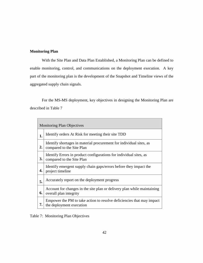
42
Monitoring Plan
With the Site Plan and Data Plan Established, a Monitoring Plan can be defined to
enable monitoring, control, and communications on the deployment execution. A key
part of the monitoring plan is the development of the Snapshot and Timeline views of the
aggregated supply chain signals.
For the MS-MS deployment, key objectives in designing the Monitoring Plan are
described in Table 7
Monitoring Plan Objectives
1. Identify orders At Risk for meeting their site TDD
2. Identify shortages in material procurement for individual sites, as compared to the Site Plan
3. Identify Errors in product configurations for individual sites, as compared to the Site Plan
4. Identify emergent supply chain gaps/errors before they impact the project timeline
5. Accurately report on the deployment progress
6. Account for changes in the site plan or delivery plan while maintaining overall plan integrity
7. Empower the PM to take action to resolve deficiencies that may impact the deployment execution
Table 7: Monitoring Plan Objectives

43
These objectives lead to the development of the Status Snapshot and the Status
Timeline dashboards, based on the data available from the data plan. As stated
previously, a primary objective of this paper is to develop a methodology for managing
MS-MS deployments that is accessible to OEM PM's without the need for advanced
databasing skills, customized application development or purchase, or complex macro
execution within a spreadsheet. The data views described below are taken from a
Microsoft Excel workbook built to execute the Data Plan defined above. For reference,
Appendix B details the architecture in that workbook. It was developed for ease of use
by a PM, but was strictly limited to standard cell-reference functions, pivot tables, and
other Excel features.
Status Snapshot
The Status Snapshot is a mechanism to provide a PM with a simple view to the
status of the deployment execution based on the most current supply chain information
available. As noted above, the Monitoring Plan includes several different objectives for
quality control and communication, each of which involves a slightly different view of
the status of a deployment. For our Case Model, the Status Snapshot needs to identify
clearly the following attributes

44
Snapshot Attribute
1. QTY of each product required by each site, per the site plan
2. QTY of each product on order for each site (Live Orders Only)
3. Health of OEM MFG Orders
4. Orders at Risk for missing their TDD
5. Have any orders been cancelled?
6. Qty of material left to Ship
7. Qty of material that has already shipped
8. Qty of Material on Live Orders compared to QTY required by the Site Plan
9. Qty of Material not yet shipped, compared to QTY required by Site Plan
Table 8 Status Snapshot Attributes
Figure 2 shows a view of the Status Snapshot for the Case Model deployment that
displays that QTY of each product type, for each site, based only on the Site Plan
(attribute 1 in Table 8). Discrete product types are shown in columns, with quantities for
each site show in each row. Note that Sites, Products, and TDD's are presented in one
view, easily consumed by the PM and other stakeholders (see Appendix B for details of
the Status Snapshot calculations and display).

45
Figure 2: Status Snapshot - Plan QTY View
Functionally, the Status Snapshot in this example is an Excel Pivot Table of the
underlying OSR data, converted into the appropriate values based on the Translator
Calculations outlined in Table 6. Using a standard pivot table provides the added
flexibility allowing the OEM PM to drill down into the individual site plan information
that is displayed in each view.

46
Attribute 2 of Table 8 calls for a Snapshot view of the Live Orders related to the
deployment. Figure 3 shows that view, based on one day's OSR. This view shows all of
the Live Orders associated with the deployment. As noted in the Data Plan, Live Orders
are any order in any production phases that have not been cancelled.
Figure 3: Status Snapshot - Live Order View

47
The data in this view is rudimentary and is simply a summary of active orders in
the supply chain, based on the OSR. Underlying this view is simply the OSR, in a flat
file format, a section of which is shown in Figure 4
Figure 4: Sample OSR Data
Customer # Customer PO # Dell Order # Invoice # Order Type Status Order Entry
Date
In Production
Date
Current Estimated Ship Date
100504440 PO-Client 719254430 Invoices Invoiced 6/16 6/20 7/18100504440 PO-enterprise 740127092 Invoices Invoiced 7/12 7/12 7/18100504440 PO-enterprise 702965182 Invoices Invoiced 5/28 5/28 7/27100504440 PO-Client 714406084 Invoices Invoiced 6/10 6/11 7/14100504440 PO-Client 713099310 Invoices In Production 6/9 6/13 7/22100504440 PO-Client 713101181 Invoices Invoiced 6/9 6/13 7/21100504440 PO-Client 713103476 Invoices Invoiced 6/9 6/13 7/21100504440 PO-Client 724371286 Invoices Cancelled 6/22 7/13100504440 PO-enterprise 724372029 Invoices Cancelled 6/22 7/8100504440 PO-Client 735709540 Invoices Invoiced 7/6 7/12 7/26100504440 PO-enterprise 735710431 Invoices Invoiced 7/6 7/12 7/15102410529 PO-Client 720739924 Invoices Invoiced 6/17 6/20 7/19102410529 PO-enterprise 720443808 Invoices Invoiced 6/17 6/18 7/7102410529 PO-Client 720450456 Invoices Invoiced 6/17 6/20 6/29102410529 PO-Client 720458913 Invoices Invoiced 6/17 6/20 6/29102410529 PO-Client 724451120 Invoices Invoiced 6/22 6/23 7/5102410529 PO-Client 725600501 Invoices Invoiced 6/23 6/24 7/6102410529 PO-enterprise 725600865 Invoices Invoiced 6/23 6/24 8/8102410529 PO-Client 726641249 Invoices Cancelled 6/24 6/26 7/26102410529 PO-enterprise 726641603 Invoices Invoiced 6/24 6/25 8/9102410529 PO-enterprise 743009669 Invoices Invoiced 7/14 7/14 7/20102410529 PO-Client 727093648 Invoices Invoiced 6/24 6/25 7/8102410529 PO-enterprise 727093689 Invoices Invoiced 6/24 6/25 8/9102410529 PO-Client 731550971 Invoices Invoiced 6/30 6/30 7/13102410529 PO-enterprise 731551169 Invoices Invoiced 6/30 6/30 7/20102410529 PO-enterprise 731554213 Invoices Invoiced 6/30 6/30 8/15102410529 PO-Client 731741281 Invoices Invoiced 6/30 7/7 7/14102410529 PO-enterprise 731741703 Invoices Invoiced 6/30 6/30 8/15

48
Independently, these views do not offer much value to the PM in monitoring and
controlling the project, but the underlying data can be exploited to present the other
attributes listed in Table 8 Status Snapshot Attributes above. By using the Translator
algorithms described in Table 6, each order in the OSR can be evaluated for TDD Risk,
Order Health, Order Status, and timeline/quantity variations against the Site Plan. By
including those calculated attributes into the Snapshot, the PM can gain quick,
consolidated view to the timeline risk of any product, for any site. Figure 5 shows a
Delta-To-Plan (DTP) view of the OSR data, indicating where product quantities for
"Live" orders do not match the Site Plan. This is a quick indication to the PM that
insufficient material orders have been placed to meet the site plan (or prior Live orders
have been cancelled), and action will be needed.

49
Figure 5: Status Snapshot - Delta to Plan
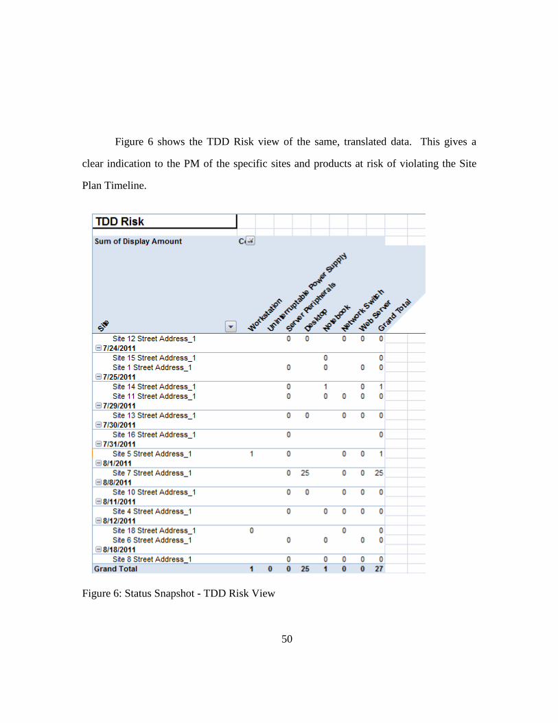
50
Figure 6 shows the TDD Risk view of the same, translated data. This gives a
clear indication to the PM of the specific sites and products at risk of violating the Site
Plan Timeline.
Figure 6: Status Snapshot - TDD Risk View

51
In similar fashion, alternate views of the translated OSR data are available for
each of the nine project attributes called out in Table 8 Status Snapshot Attributes. With
this snapshot capability, each recurring OSR can be evaluated independently to determine
near term and long term risk to the deployment schedule. Changes to the Site Plan, and
Manual Updates can also be correlated to any individual OSR to ensure that the most
recent, accurate data is available to the PM.
Status Timeline
The Status Snapshot gives an instantaneous picture of the status and risks
associated with the MS-MS Deployment. Over time, though, a PM will also be obligated
to show progress trends in the execution of a deployment (PMI, 2008). Reporting
requirements for a deployment can require recurring updates on completed activities,
progress on open items, and root-cause discussions on missed milestones. At the same
time, the Snapshot can identify orders that have been cancelled and material quantities
that do not meet the Site Plan requirements, but it does give the OEM PM a clear picture
in examining what caused a gap in material availability. The Status Timeline allows a
long term, historical view of the deployment to be developed in order to address these
kinds of requirements. For our Case Model, the Status Timeline needs to identify clearly
the attributes shown in Table 9.

52
Timeline Attribute
1. QTY of each product on order for each site, over time
2. Live Order QTY Delta to Plan, over time
3. Qty of At Risk orders, over time
4. Indication of when a Live Order Qty is reduced, indicating an order was cancelled and generally requiring attention
Table 9: Status Timeline Attributes
The Status Timeline is developed by recording the Snapshot values each time an
OSR is generated, and time stamping when those values are generated. This is a
straightforward process in a spreadsheet format by simply copying the relevant, translated
data from the OSR into a static location, and adding additional data when available. This
is a manual process, however, and must be executed diligently by the PM in order to
build up the overall timeline picture. More sophisticated methods are available through
relational databases and fully developed toolsets <cite examples>, but the intention of
this paper is to develop a PM owned process that does not rely heavily on complex data
management tools. Figure 7 shows the Status Timeline for the Case Model, including
trend tracking.

53
Figure 7: Status Timeline Sample
Snapshot date -->
QTY Live In Plan
Net delta to plan
Live @ Risk
QTY Live In Plan
Net delta to plan
Live @ Risk
QTY Live In Plan
Net delta to plan
Live @ Risk
Totals 470 630 10 511 589 11 516 584 2Trend day 0 day 0 10 41 -41 1 5 -5 -9
Site Product QtySite 1 Street Address_1 Desktop 95 0 -95 0 19 -76 0 19 -76 0Site 1 Street Address_1 Network Switch 75 0 -75 0 0 -75 0 0 -75 0Site 1 Street Address_1 Notebook 200 107 -93 0 107 -93 0 107 -93 0Site 1 Street Address_1 Server Peripherals 3 1 -2 0 1 -2 0 1 -2 0Site 1 Street Address_1 Web Server 2 0 -2 0 0 -2 0 0 -2 0Site 10 Street Address_1 Desktop 11 1 -10 1 1 -10 1 1 -10 0Site 10 Street Address_1 Network Switch 2 1 -1 0 1 -1 0 1 -1 0Site 10 Street Address_1 Server Peripherals 1 0 -1 0 0 -1 0 0 -1 0Site 10 Street Address_1 Web Server 1 0 -1 0 0 -1 0 0 -1 0Site 11 Street Address_1 Network Switch 2 1 -1 0 1 -1 0 1 -1 0Site 11 Street Address_1 Notebook 51 1 -50 1 1 -50 1 1 -50 0Site 11 Street Address_1 Server Peripherals 3 0 -3 0 0 -3 0 0 -3 0Site 11 Street Address_1 Web Server 3 0 -3 0 0 -3 0 0 -3 0Site 12 Street Address_1 Desktop 6 1 -5 0 1 -5 0 1 -5 0Site 12 Street Address_1 Network Switch 2 1 -1 0 1 -1 0 1 -1 0Site 12 Street Address_1 Server Peripherals 4 1 -3 0 1 -3 0 1 -3 0Site 12 Street Address_1 Web Server 2 0 -2 0 0 -2 0 0 -2 0Site 13 Street Address_1 Desktop 17 3 -14 3 3 -14 3 2 -15 0Site 13 Street Address_1 Network Switch 10 3 -7 0 3 -7 0 3 -7 0Site 13 Street Address_1 Server Peripherals 1 0 -1 0 0 -1 0 0 -1 0Site 13 Street Address_1 Web Server 1 0 -1 0 0 -1 0 0 -1 0Site 14 Street Address_1 Notebook 13 1 -12 0 1 -12 0 1 -12 1Site 14 Street Address_1 Server Peripherals 3 0 -3 0 0 -3 0 0 -3 0Site 14 Street Address_1 Web Server 3 0 -3 0 0 -3 0 0 -3 0Site 15 Street Address_1 Network Switch 1 1 0 0 1 0 0 1 0 0Site 15 Street Address_1 Notebook 23 11 -12 0 11 -12 0 11 -12 0Site 16 Street Address_1 Notebook 200 200 0 0 200 0 0 200 0 0Site 16 Street Address_1 Server Peripherals 3 1 -2 0 1 -2 1 1 -2 0Site 17 Street Address_1 Notebook 23 1 -22 0 1 -22 0 1 -22 0Site 17 Street Address_1 Web Server 2 1 -1 0 1 -1 0 1 -1 0Site 18 Street Address_1 Network Switch 2 1 -1 0 1 -1 0 1 -1 0Site 18 Street Address_1 Workstation 4 0 -4 0 0 -4 0 0 -4 0Site 19 Street Address_1 Uninterruptable Pow 2 0 -2 0 0 -2 0 0 -2 0Site 19 Street Address_1 Workstation 3 1 -2 0 1 -2 0 1 -2 0Site 2 Street Address_1 Network Switch 42 42 0 0 42 0 0 40 -2 0Site 2 Street Address_1 Notebook 55 55 0 0 55 0 0 55 0 0Site 2 Street Address_1 Server Peripherals 3 2 -1 0 2 -1 0 2 -1 0Site 2 Street Address_1 Workstation 4 2 -2 0 2 -2 0 2 -2 0Site 20 Street Address_1 Notebook 21 10 -11 0 10 -11 0 10 -11 0Site 21 Street Address_1 Desktop 10 5 -5 5 5 -5 5 5 -5 0Site 21 Street Address_1 Network Switch 6 5 -1 0 5 -1 0 5 -1 0Site 22 Street Address_1 Network Switch 1 1 0 0 1 0 0 1 0 0Site 22 Street Address_1 Notebook 9 1 -8 0 1 -8 0 1 -8 0Site 3 Street Address_1 Server Peripherals 1 0 -1 0 0 -1 0 1 0 0Site 4 Street Address_1 Network Switch 6 3 -3 0 3 -3 0 3 -3 0Site 4 Street Address_1 Notebook 48 3 -45 0 3 -45 0 3 -45 0Site 4 Street Address_1 Server Peripherals 2 0 -2 0 0 -2 0 0 -2 0Site 4 Street Address_1 Web Server 2 0 -2 0 0 -2 0 0 -2 0Site 5 Street Address_1 Network Switch 1 0 -1 0 0 -1 0 1 0 0Site 5 Street Address_1 Server Peripherals 1 0 -1 0 0 -1 0 0 -1 0Site 5 Street Address_1 Web Server 1 0 -1 0 0 -1 0 0 -1 0Site 5 Street Address_1 Workstation 4 0 -4 0 0 -4 0 1 -3 1Site 6 Street Address_1 Notebook 15 1 -14 0 1 -14 0 1 -14 0Site 6 Street Address_1 Server Peripherals 5 1 -4 0 1 -4 0 1 -4 0Site 6 Street Address_1 Web Server 3 0 -3 0 0 -3 0 0 -3 0Site 7 Street Address_1 Desktop 25 0 -25 0 0 -25 0 0 -25 0Site 7 Street Address_1 Network Switch 2 0 -2 0 0 -2 0 0 -2 0Site 7 Street Address_1 Server Peripherals 2 0 -2 0 0 -2 0 0 -2 0Site 7 Street Address_1 Web Server 2 0 -2 0 0 -2 0 0 -2 0Site 8 Street Address_1 Network Switch 22 0 -22 0 11 -11 0 11 -11 0Site 8 Street Address_1 Notebook 22 0 -22 0 11 -11 0 11 -11 0Site 8 Street Address_1 Server Peripherals 1 0 -1 0 0 -1 0 0 -1 0Site 8 Street Address_1 Web Server 1 0 -1 0 0 -1 0 0 -1 0
5-Jul 10-Jul
Site Plan Status Timeline
19-Jul

54
This timeline view was developed by extracting the Live Quantity of product
orders for each site, and each product type, from the Snapshot View. The data is tagged
to show the date that the Snapshot was taken, and summary calculations display the Net
order quantity differences between live order volumes and the Site Plan requirements.
Net (calculated as the sum of the Absolute Value of the difference between Live QTY
and Site Plan QTY). Over time (moving to the right in the timeline view) you can see the
total Live order quantity for all products increasing as more orders are place to meet the
Site Plan requirements. "At Risk" volumes are also tracked, showing changes as the
OEM PM takes actions to either accelerate deliveries or adjust the site plan. Over the
entire duration of the deployment, the volumes of each of these attributes can be charted
and used to show progress through the site plan and measures of average At-Risk
volumes. Additionally, each site and each product are tracked over time, enabling the
OEM PM to deliver site specific reporting to show progress or challenges against
individual Site requirements. Individually, as shown in Figure 7, simple color coding
through Conditional Formatting can help a PM identify exactly when changes in Live
QTY are made, enabling them to troubleshoot gaps in the delivery timeline due to
unexpected changes in the supply chain.
Cyclic Routine
With the Site Plan, Data Plan, and Monitoring plans in place, execution of the
initial product orders can begin. As orders are entered into the OEM Order Management
System (unique per OEM), demand signals will flow through normal channels into the
supply chain. For Dell, the OSR data is available once orders are placed, and as the
manufacture and fulfillment mechanisms begin to execute, updates will begin to be

55
reflected in the OSR. To tap into that data, then, and begin to leverage the Snapshot and
Timeline dashboards, the OEM PM will need to establish a standard cyclic routine.
Based on the Data plan (and related spreadsheet dashboards) created for the case model
the PM will need to execute the steps in Table 10 each time new data is available.
PM Cyclic Routine
1. Obtain new OSR or specific manually tracked data
2. Verify the data meets the Data Plan requirements (exa. no duplicated order numbers in the OSR, manually entered ship method has a defined transit time)
3. Copy the OSR into the data input section of the dashboard workbook (Or add data to the Manual Data Tab, per the Manual Input Method)
4. Refresh All Pivot tables
5. Validate Data Integrity by verifying sums: Does total product quantity match known numbers? do site quantities/names still match Site Plan (this step is to ensure the new data was accurately added to the workbook)
6. Update the Timeline View to record the new data.
7. Compare the new Timeline view to the Snapshot to verify they show the same data (another validation checkpoint to ensure data integrity, both views should match at the time new data is added)
8. Analyze each view of the Snapshot to determine project progress, identify risks, identify supply chain anomalies
9. Use the updated Snapshot and Timeline data to execute communications, change management, and corrective actions per the established project plan
Table 10: OEM PM Cyclic Routine

56
Chapter 6: Summary and Conclusions
PROJECT MANAGEMENT APPLICATIONS
In prior sections, I presented a series of concerns and complications that can cause
a Multi-Source, Multi-Site deployment to miss key timeline and cost targets. The
Methodology in Chapter 5: Managing the Multi-Source, Multi-Site Deployment Data was
designed to assist a PM is filtering through recurring Supply Chain status reports to
develop a comprehensive view of an ongoing execution. That information alone does will
not drive a successful deployment, and the PM is challenged with leveraging that
information to make decisions, influence stakeholders, and manage resources as
necessary to meet the overall program targets.
The Project Management Institute <PMBOK> groups much of the key actions
necessary to execute a MS-MS deployment into the "Executing" and "Monitoring and
Controlling" process groups. These groups of activities are described as "the process of
tracking, reviewing, and regulating the progress to meet the performance objectives
defined in the project management plan". In the specific case of MS-MS deployments,
the Site Plan described above is one element of the overall project plan, and the Status
Snapshot and Timeline dashboards represent part of the tools and techniques available to
the PM to help Direct and Manage the Project Execution. These components, however,
are only a subset of the overall planning and execution mechanisms necessary for a
successful deployment. If developed and implemented fully during a deployment, the
dashboards can also support aspects of Project Time Management, Communications
Management, and Risk Management, as described in the PMBOK.

57
PMI also categorizes actions taken to effect changes in the direction of a project
as Corrective Actions, Preventive actions, and Defect Repair. The methodology defined
above for MS-MS deployments can provide indicators of at-risk orders, and missed
deadlines that can enable actions in each of those 3 categories. One key attribute of the
MS-MS deployment method is the ability to identify, but target site, what dates on a
deployment schedule are at risk. While corrective and preventive actions can be taken to
adjust schedule risks by manipulating the supply chain, the dashboards also provide an
easily consumable overview of project progress that can facilitate changes to the Site
Plan (Project Schedule) through a formal change control process. By identifying and
grouping sites that will be challenged to execute as scheduled, the Site Plan can be
adjusted to focus resources onto sites that are at lower risk rather than taking the more
costly route of accelerated shipping and expedited manufacture.
In the Last Planner method of project management, the PMI concepts of project
control are examined and described as largely ineffectual. Ballard characterizes the PMI
approach by noting that for the PMI, "project control consists of monitoring progress
toward project objectives and taking corrective action when the ship appears to be off
course… The objective is to detect negative variances from target, so corrective action
can be taken". He suggests taking a "Production Control" approach in which actions are
taken to meet the prerequisites of scheduled work before it is allowed to proceed. This is
in contrast to the Project Control approach, where work is driven to execute on the
project schedule, and corrective actions are taken as necessary when indications show
that specific tasks are not proceeding as expected. As applied to the MS-MS deployment,
the concept in the Last Planner system is that a Site would not be scheduled for
installation until all pre-requisites for the technical work are met. Specifically, Sites
would not be scheduled for deployment until all material procurement for that site is

58
delivered. As noted earlier, having the material on site for too long, however, causes risk
to the material and impact to the customer's business operations. Leveraging the Status
Snapshot and Timeline developed in Chapter 5, however, it is conceivable that a balance
can be maintained where a Site is not scheduled for deployment until all material reaches
a pre-determined status in the supply chains. With slight modifications, the MS-MS
process can be adapted to identify sites that are "X" or more days from being delivered
complete, at which point the site is actually scheduled for technicians to arrive and
deploy gear. Within a window defined by production lead times and average transit
times (already components of the MS-MS process), the value of X (days until material is
on-site) can be set as part of the project plan. With that established, a cyclic routine can
be envisioned whereby specific sites are scheduled (within the context of a broader
timeline) based on actual supply chain progress, instead of attempting to bend the global
supply chain to meet a pre-defined Site schedule. By accepting the variability present in
supply chain execution, the risk of having technicians on-site without the proper
equipment to complete the technology installation can be reduced.
SUMMARY
The Multi-Source, Multi-Site deployment is a complex balance of multiple
competing timelines that can be affected by a wide variety of influences. Perturbations in
global supply chains, manufacturing schedules, and local shipping capacities insert
variations in cycle times that OEM's experience between receiving an individual
customer orders and delivering product on site. Those variations are compounded when
attempting to control delivery activities within small time windows across a variety of
products supplied by multiple vendors. It is the task of a deployment project manager to

59
interpret a variety supply chain signals and identity any risks in meeting defined delivery
schedules. Additionally, each MS-MS deployment will have different customer
requirements, site requirements, and timeline pressures. With that amount of variability,
the PM will benefit from a structured approach to defining what supply chain data is
available and how it can be used to help manage expectations, monitor execution, and
effect the overall deployment success.
In this paper, I presented an approach that breaks the planning into 3 primary
deliverables; the Site Plan, the Data Plan, and the Monitoring Plan. Executing those three
plans will drive a PM to understand the supply chain data available to them, translate that
data into information useful and understandable by all stakeholders, and monitor the
progress of the supply chain against the deployment schedule. In practical terms, those
plans culminate in a data mining and data management methodology that can be
supported with spreadsheet based dashboards that provide both a fixed Snapshot of the
status of the deployment as well as a Timeline of key material movements over the
duration of the deployment.
The Status Snapshot and Timeline provide information to the PM that will give
them insight into timeline risks and supply chain challenges. Incorporating that
information into the overall Project Management methodology was not explored in this
paper, and is a valid topic for further investigation. With a clearer picture of supply chain
execution, however, a PM tasked with a Multi-Source, Multi-Site deployment can better
leverage existing project change controls to improve their chances of successfully
meeting their schedule and cost targets.

60
Appendix A: Project Scoping Framework
Table A1 lists standard project scoping questions that solution architects use
today to understand the details of a managed customer engagement. These questions
cover a wide range of potential support activities, including the underlying risks of MS-
MS Deployments.
Project Scoping Framework
Is this engagement the result of RFP/RFQ or RFI?
Is this project customer facing?
Intake Mgr has scoped/received SOW approval?
Has Intake Mgr confirmed Ops PM deliverables?
Is a re-scope required after project kickoff meeting?
Has the project qty been confirmed? Project vs. Run Rate?
Has the project timeline been confirmed?
Has the preliminary project been loaded into Sharepoint?
Is this a project renewal or refresh of an existing project?
Has the project been assigned to an Ops PM?
Has there been an Ops PM pricing agreement? (per unit, per quarter, or per month?
Was the customer quoted prior to PM engagement?
Project Specific Details
Does this project/program involve a reseller? (Who?)
Is there Alliances involvement (GD, LM, NG)?
Is the customer's project funded?
Is any element of the project restricted to US only citizens?
Will any product be shipped OCONUS? Where?
Will purchases be project or run rate based?
Is the LOT qty and probability accurate in SFDC?
Who is the finance person for this project?
Does the customer encourage direct contact with the PM?
Will DOD UID labeling be required on any or all equipment?

61
Project Scoping Framework
Is EPEAT and/or ESTAR a requirement for the equipment?
Known contract vehicle for this project (SEWP, ITES, GSA?
Pre-Order Solutioning
B2B, Premier or Global Portal requirements? Is it new or existing?
Is there a contractual SLA? What is it? Is SLA Mgr. engaged?
Is there a dedicated ASR or OP for this customer project?
Order Placement: Bulk vs. Staggered
Will the project span a product transition?
Will integrator or vendor management be required? Who?
Has there been a partner agreement or SOW provided?
Custom Factory Integration
Is CFI required on the project? Who is the CFI PM?
Is a customer provided or custom image required?
Asset tags required: consigned or Dell managed?
Hardware integration (DiB): S&P or Dell branded
Is CFI reporting needed for IP addresses, or product info?
Custom Fulfillment Solutions (CFS)
Does product need consolidation, tagging, RNS, etching, or other CFS services?
Shipping & Delivery requirements
Will the project require delayed or staggered delivery?
Are special carriers or white glove delivery services required? Consolidated, staggered delivery or basic build and ship?
Is the customer requiring special OCONUS deliveries?
Any other special delivery requirements (date-specific, time-specific, inside delivery, etc)?
Invoicing
Does the customer have special invoice requirements?
Custom invoices: Do they requires Controller approval?
What is the customer's net terms?
Will PM intervention be needed to meet invoicing requirements?
Reporting
Are there any reporting requirements for the project?
Is a custom report being managed today? Example of report?

62
Project Scoping Framework
CARS: Self Serve
Custom Reporting
Communication
Is there a preference in establishing a weekly call?
Who is the preferred lead PM when managed services is engaged? Sales Ops or Services?
Managed Services
Does this project involve Managed Services?
Are services being performed by Dell? Other?
Who is the Services PM for this project/program?
Table A1: Project Scoping Framework

63
Appendix B: The MS-MS Status Snapshot
A primary objective of this paper is to develop a methodology for managing MS-
MS deployments that is accessible to OEM PM's without the need for advanced
databasing skills, customized application development or purchase, or complex macro
execution within a spreadsheet. The concepts presented in this paper are general enough
to apply to a variety of deployment activities, but the OEM PM needs a simplified
method for applying those concepts in order to have a direct impact. The workbook
architecture presented here is the foundation that a Dell PM can use to implement the
Monitoring Plan described earlier, using the OSR as the baseline source data. It was
developed for ease of use by a PM, but was strictly limited to standard cell-reference
functions, pivot tables, and other Excel features.
To operationalize the Data Plan described in Chapter 5, the MS-MS workbook
must incorporate a Translator and a Manual Input Method for manipulating the source
data. At the same time, the workbook should be flexible enough to accept variations in
the source data and robust enough to preserve information even if inaccurate, or "bad"
data is inserted. To that end, the following philosophies apply:
1. Updating the OSR data should involve only importing a whole worksheet. Errors
are too easily inserted if a PM is required to routinely select specific cells within a
worksheet to cut & paste into another
2. The OSR data should not be changed by the process. It should serve as a fixed
input

64
3. The PM should not be required to perform any Cell manipulations to update the
workbook. Changing cell references, formulas, or content will eventually result
in errors compounded through the deployment
4. The Workbook should provide some forms of "checksums", general data integrity
validations that provide feedback to a PM that the data is reliable
5. Output views should be easily copied to other standard formats for outbound
reporting to stakeholders via the Project Communications Plan
6. Any pivot tables should have very limited filters and require limited interaction
from the PM, so that all data in the OSR is accounted for. Filtering out data can
mask unpredictable errors
7. Any error checking should provide obvious indications to the PM that there are
issues in the data stream that should be investigated. Care must be taken when
masking Lookup and Reference failures with IFERROR and ISERROR functions
With those concepts in mind, the MS-MS Workbook was developed as follows
1. Establish the Site Plan: One sheet in the MS-MS workbook contains the site plan.
This is a flat presentation of the plan with only key data present, but with no gaps in
the spreadsheet. This sheet should involve no functions or calculations and holds
the latest approved plan. A Pivot of this table can be generated to provide a more
visually pleasing view of the data, but the Plan should be maintained accurately in
this flat format (Figure B1). Note, updates to the site plan in this format can be
cumbersome, care must be taken to ensure that all records for each site reflect the
same TDD.

65
Figure B1: Site Plan in MS-MS Workbook
2. Update the OSR Data: The OSR is a report generated by Dell's internal reporting
systems and delivered to a PM as a worksheet attachment to an email. Typically,
this is a daily report. The OSR data occupies one worksheet in the MS-MS
Workbook (the 'Current Status" tab) and is imported by selecting all the data from
the original OSR worksheet and pasting it into the MS-MS workbook. No other
manipulations are required.
3. Populate the Order Checker: Identify relevant columns in the OSR, and port that
data into a separate worksheet through simple Offset and Match functions. 'Order
Checker' is a sheet in the MS-MS workbook that consolidates data and allows for
calculations. The structure used here requires that the column headings in the Order
Checker sheet match exactly the text of the column headings in the OSR. The
SiteCustomer
PO #Target On-Site date QTY Product Line
Site 1 Street Address_1 PO-Client 7/24 95 DesktopSite 1 Street Address_1 PO-enterprise 7/24 75 Network SwitchSite 1 Street Address_1 PO-Client 7/24 200 NotebookSite 1 Street Address_1 PO-enterprise 7/24 3 Server PeripheralsSite 1 Street Address_1 PO-enterprise 7/24 2 Web ServerSite 10 Street Address_1 PO-Client 8/8 11 DesktopSite 10 Street Address_1 PO-enterprise 8/8 2 Network SwitchSite 10 Street Address_1 PO-enterprise 8/8 1 Server PeripheralsSite 10 Street Address_1 PO-enterprise 8/8 1 Web ServerSite 11 Street Address_1 PO-enterprise 7/25 2 Network SwitchSite 11 Street Address_1 PO-Client 7/25 51 NotebookSite 11 Street Address_1 PO-enterprise 7/25 3 Server PeripheralsSite 11 Street Address_1 PO-enterprise 7/25 3 Web ServerSite 12 Street Address_1 PO-Client 7/23 6 DesktopSite 12 Street Address_1 PO-enterprise 7/23 2 Network SwitchSite 12 Street Address_1 PO-enterprise 7/23 4 Server Peripherals

66
column order in the OSR can vary, based on options selected by the PM, so I
developed the workbook to allow for the columns to exist in any order in the OSR
This was accomplished as follows:
a. Figure B2 shows the section of the Order Checker worksheet containing a view
to the OSR data. The header row (1:1) contains the exact text of the columns in
the OSR that are needed. Each cell below contains the formula below:
Figure B2: Order Checker with OSR Data
'Current Status' is the worksheet that contained the OSR data. This populates
each cell with the related OSR data, based on matching the heading in the OSR
to the heading in the Order Checker tab. This formula is copied down to row
2000 in the order checker sheet, allowing for up to 2000 records to be present in
the OSR. Rows below 2000 are used for other information as described below.

67
b. The Order Checker sheet also needs to contain the Site Plan data. Having both
the OSR data and the Site Plan data in one sheet facilitates some presentation
functions later without needing specialized macros. Site plan data is loaded into
the Order Checker sheet starting at row 2000, using simple lookups, shown in
Figure B3
Figure B3: Order Checker with Site Plan Data
'Site Plan' is the sheet in the MS-MS workbook where the Site Plan (Figure B1)
resides.
4. Establish the Translator: With the OSR data and Site plan data ported into the Order
Checker sheet, the next step is to apply the analytics defined in the data plan.
Several constants were defined in the data plan, and those are maintained in the
'Translator' sheet (Figure B4). They include the Transit Time associated with each
Ship Method, the allowable dwell time in "IP" status before an order is considered
unhealthy, and the Early/Late delivery window that establish when an order is at
risk.

68
Figure B4: The Translator Worksheet
5. Perform Translations: Within the Order Checker sheet, calculations can be made on
the OSR data and the Plan data to determine the translated Status of each individual
order. Figure B5 shows a sample of the resulting data
Figure B5: Applied Translations in the Order Checker
Calculations for each field include error checking and data smoothing designed to
deliver useful output to the PM. The TDD-at-Risk calculation, for example, is
Order Snapshot ValidationShip Method Transit Time note- ship method must match data stream text exactlyLTL 3 to 5 days service 5 This is a lookup table that drives EDD calculationsNext Day 2
Health Check 7 <-- Max number of days IP to be a healthy orderTimeline risk if EDD>TDD by 0 days or more late, "0" means it cannot be late by even 1 dayTimeline risk if EDD<TDD by 10 days or more early

69
shown for cell M3. The results on the right hand cells in figure B5 are
summations of the quantities of each order that apply to each category, based on
the translations (translations highlighted in yellow). Similar calculations are
performed against each item in the Site Plan, in rows 2000 and below on the
Order Checker sheet. The "Delta to Plan" (DTP) columns are calculated against
the plan data, not the OSR order data.
6. Display the Status Snapshot: With the Translation calculations completed in the
Order Checker tab, status results can be presented to the PM. This is done through
a Pivot of the data in the Order Checker sheet. One of the goals here was to keep
the manipulations required of the PM to a minimum, but also present the
information as concisely as possible. The result was a single sheet that allows
multiple views of the status information (screen shots were presented in Chapter 5).
To enable that functionality, a pull-down menu is presented to the PM on the
Snapshot sheet that allows the PM to select the view they want. Note, this is not a
Pivot Table Page Filter, but was designed to look similar, see Figure B6.
Figure B6: Snapshot Menus
Menu of available views

70
Once a view is selected, a separate VLOOKUP reference is made to determine
what data in the Order Checker the PM is looking for. Each selection in the view
menu is mapped to a specific column in the Order Checker, and the data in that
column is used in the final Status Snapshot Pivot (Figure B7).
Figure B7: Snapshot Data Mapping
View Map in the Data Plan Sheet
Drives "Display Amount" in the Order Checker

71
This mapping and reference-based data population is a bit cumbersome to establish
initially, but accomplishes the goals of limiting the amount of interaction the PM
must have with the underlying data and logic in order to get the relevant Snapshot
data.
The workbook architecture presented above requires some specific data controls,
but in execution on the PM's cyclic routine (as defined as part of the Monitoring plan)
there are minimal requirements for a PM to extract useful information. This structure
also adds some flexibility including the ability to accept various OSR reporting (column
sequence doesn’t matter, and the headers are defined as corporate reporting standards that
cannot be changed). Also changes to the Site plan are automatically incorporated into the
reporting, and adjustments can be made easily to the definitions of At-Risk orders and
unhealthy orders.
Using this framework, additional calculations can easily be added to the
Translator and Order Checker to provide additional views of the OSR and Site Plan
information directly into the existing Snapshot display.

72
References
Amaral, J., Billington, C., Tsay, A. (2006). "Safeguarding the Promise of Production Outsourcing". Interfaces, Vol. 36, No. 3, May–June 2006, pp. 220–233
Askegar, V., (2004). "The Demand Driven Supply Network". Supply Chain Management Review, April 2004.
Atallah, M., Blanton, M., Frikken, K. (2010). "Outsourcing Manufacturing: Secure Price-Masking Mechanisms for Purchasing Component Parts". Production and Operations Management, Vol. 20, No. 2, March–April 2011, pp. 165–180.
Ballard, H. G., (2000). "The Last Planner System of Production Control". Thesis submitted to School of Civil Engineering, The University of Birmingham.
Beck, M., (2011). "Cost Effective Refresh Cycles". Beckon Online, Technology, Jan 11, 2011
Dell Inc., (2008). "Streamlining Client Migration and Deployment". Dell Power Solutions, May 2008, pp. 96.
Dell Inc., (2007). "Client Deployment Assessment". Service Definition and Deliverables, Dell Inc., Round Rock, TX.
Evrard-Samuel, K. (2008). "Sharing Demand Signals: A New Challenge to Improve Collaboration within Supply Chains". Supply Chain Forum, Vol. 9 - No 2.
Fan, W., Geerts, F., Li, J., Xiong, M. (2011). "Discovering Conditional Functional Dependencies". IEEE Transactions On Knowledge And Data Engineering, Vol. 23, No. 5.
Gaukler, G., Özer, O., Hausman, W. (2008). "Order Progress Information: Improved Dynamic Emergency Ordering Policies". Production and Operations Management, Vol. 17, No. 6, November–December 2008, pp. 599–613.
Healy, M., (2010). "Dell PC Optimized Deployment Model". International Data Corporation, Framingham, MA.
Insight (2005), " Managed Pc Refresh: The Clear Path to Enterprise PC Refresh". White Paper prepared by Insight, Tempe AZ.
Karkkainen, M., Ala-Risku, T., Framling, M. (2003). "Efficient tracking for short-term multi-company networks". International Journal of Physical Distribution & Logistics Management Vol. 34 No. 7, pp. 545-564.
Lee, H., Padmanabhan, V., Whang, S., (2004). "Information Distortion in a Supply Chain: The Bullwhip Effect". Management Science, Vol. 50, No. 12 Supplement, December 2004, pp. 1875–1886

73
Project Management Institute, Standards Committee (2008). "A Guide to the Project Management Body of Knowledge Fourth Edition". Project Management Institute, Newton Square, PA.
Ragurathan, R., (2009). "How to Develop a Supply Chain-Friendly Network". Industry Week, May 2009, Penton Publishing, pp. 46-47.
Razavi, S. N., Hass, C. (2010)."Multisensor Data Fusion For On-Site Materials Tracking In Construction". Automation in Construction, Vol. 19, 1037–1046.
Sethi, S., Yan, H., Zhang, H., Zhou, J. (2007). "A Supply Chain with a Service Requirement for Each Market Signal". Production and Operations Management Vol. 16, No. 3, May–June 2007, pp. 322–342.
Tu, Y., Piramuthu, S. (2011). " A Decision-Support Model for Filtering RFID Read Data in Supply Chains". Ieee Transactions On Systems, Man, And Cybernetics—Part C: Applications And Reviews, Vol. 41, No. 2.
Williams, J., (2011). "PC market decline casts doubt on future of corporate PC refresh cycle". Computer Weekly, Desktop Computing, May 24, 2011.