efficient 3d scene labeling using fields of trees - robotics

000001002003004005006007008009010011012013014015016017018019020021022023024025026027028029030031032033034035036037038039040041042043044045046047048049050051052053

054055056057058059060061062063064065066067068069070071072073074075076077078079080081082083084085086087088089090091092093094095096097098099100101102103104105106107

ICCV#1603

ICCV#1603

ICCV 2013 Submission #1603. CONFIDENTIAL REVIEW COPY. DO NOT DISTRIBUTE.

Efficient 3D Scene Labeling Using Fields of Trees

Anonymous ICCV submission

Paper ID 1603

Abstract

We address the problem of 3D scene labeling in a struc-tured learning framework. Unlike previous work which usesstructured Support Vector Machines, we employ the recentlydescribed Decision Tree Field and Regression Tree Fieldframeworks, which learn the unary and binary terms of aConditional Random Field from training data. We showthis has significant advantages in terms of inference speed,while maintaining similar accuracy. We also demonstrateempirically the importance for overall labeling accuracy offeatures that make use of prior knowledge about the coarsescene layout such as the location of the ground plane. Weshow how this coarse layout can also be estimated by ourframework automatically, and that this information can beused to bootstrap improved accuracy in the detailed label-ing.

1. IntroductionInteracting with the world requires both an understand-

ing of the 3D geometry of a scene and of its semantic mean-ing. Remarkable achievements have been made in both ofthese directions, with systems like PTAM [8], DTAM [9]and KinectFusion [10] able to provide 3D information inreal time. Learning and inference models such as SupportVector Machines and Random Forests [3] have been usedin combination with Conditional Random Fields [2, 11] toinfer semantic labels in a range of problems. However onlyrecently has work focused on the combination of 3D dataand semantic labeling. For a successful integration of thetwo parts, the 3D representation has to be rich enough toprovide an actual benefit for the task of scene labeling, andthe scene labeling system has to be fast enough to allowinteraction with the inferred labels.

We contribute in four different ways to the combinedtreatment of reconstruction and interpretation of scenes.First, we present a framework to employ Decision TreeFields [11] and Regression Tree Fields [6] for the 3D scenelabeling task. Second, we show that both of these classi-fiers are very competitive or even outperform state-of-the-

art methods with the additional benefit of significantly fasterinference steps. Third, we compare the two classifiers in thecontext of scene labeling. And finally we use an adaptationof the framework to estimate the coarse scene layout andground plane, which are a prerequisite for high level fea-tures commonly used for 3D scene labeling.

1.1. Related Work

With the introduction of the Kinect sensor a significantnumber of works has been published on semantic labelingof RGB images with additional depth information [15, 13].While these works achieve impressive results, they focus onsemantic segmentation of single images merely using depthas an additional information source. They do not considermechanisms for consistent labels in sequences of imagesfrom cameras progressively exploring an environment.

A similar segmentation task was investigated in [12],where multiple segmentations are computed independentlyfor each image in a sequence. However, a significant im-provement of the performance is observed by enforcingtemporal consistency, which the authors achieve with aMarkov Random Field that links segments in different im-ages if they occupy the same location in 3D space.

The closest work to ours is presented in [2]. The authorsfirst integrate the 3D information from multiple images intoa single 3D point cloud and then oversegment and label thispoint cloud using full 3D geometry information. The down-side of their SVM-based approach is the processing time,which is far from real-time for their full scale classificationmodel and an accelerated, approximate solution only comesat the expense of reduced labeling performance.

We pose the problem instead within the framework ofthe recently introduced Decision Tree Fields [11] and Re-gression Tree Fields [6]. We show that this enables us todiscover consistent scene labels for a full 3D model at in-teractive rates while still maintaining the high precision andrecall of the current state-of-the-art methods.

Like many scene labeling systems, the performance ofour framework crucially relies on knowledge of the coarsescene layout comprising of a ground plane and the walls,which allows us to exploit rich geometric constraints that

1

108109110111112113114115116117118119120121122123124125126127128129130131132133134135136137138139140141142143144145146147148149150151152153154155156157158159160161

162163164165166167168169170171172173174175176177178179180181182183184185186187188189190191192193194195196197198199200201202203204205206207208209210211212213214215

ICCV#1603

ICCV#1603


yi

yi

yi

yi yi

yi

yi

yi

yi yi

yi

yi

yi

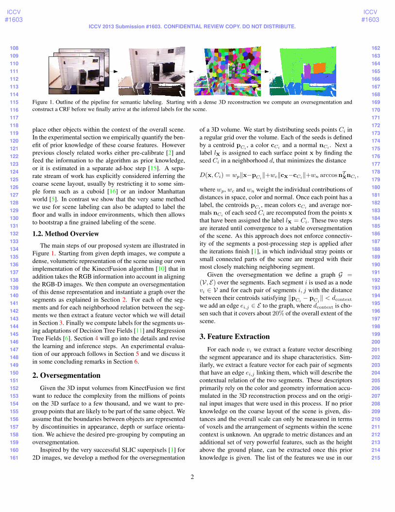
Figure 1. Outline of the pipeline for semantic labeling. Starting with a dense 3D reconstruction we compute an oversegmentation andconstruct a CRF before we finally arrive at the inferred labels for the scene.

place other objects within the context of the overall scene.In the experimental section we empirically quantify the ben-efit of prior knowledge of these coarse features. Howeverprevious closely related works either pre-calibrate [2] andfeed the information to the algorithm as prior knowledge,or it is estimated in a separate ad-hoc step [15]. A sepa-rate stream of work has explicitly considered inferring thecoarse scene layout, usually by restricting it to some sim-ple form such as a cuboid [16] or an indoor Manhattanworld [5]. In contrast we show that the very same methodwe use for scene labeling can also be adapted to label thefloor and walls in indoor environments, which then allowsto bootstrap a fine grained labeling of the scene.

1.2. Method Overview

The main steps of our proposed system are illustrated inFigure 1. Starting from given depth images, we compute adense, volumetric representation of the scene using our ownimplementation of the KinectFusion algorithm [10] that inaddition takes the RGB information into account in aligningthe RGB-D images. We then compute an oversegmentationof this dense representation and instantiate a graph over thesegments as explained in Section 2. For each of the seg-ments and for each neighborhood relation between the seg-ments we then extract a feature vector which we will detailin Section 3. Finally we compute labels for the segments us-ing adaptations of Decision Tree Fields [11] and RegressionTree Fields [6]. Section 4 will go into the details and revisethe learning and inference steps. An experimental evalua-tion of our approach follows in Section 5 and we discuss itin some concluding remarks in Section 6.

2. OversegmentationGiven the 3D input volumes from KinectFusion we first

want to reduce the complexity from the millions of pointson the 3D surface to a few thousand, and we want to pre-group points that are likely to be part of the same object. Weassume that the boundaries between objects are representedby discontinuities in appearance, depth or surface orienta-tion. We achieve the desired pre-grouping by computing anoversegmentation.

Inspired by the very successful SLIC superpixels [1] for2D images, we develop a method for the oversegmentation

of a 3D volume. We start by distributing seeds points Ci ina regular grid over the volume. Each of the seeds is definedby a centroid pCi

, a color cCiand a normal nCi

. Next alabel lx is assigned to each surface point x by finding theseed Ci in a neighborhood d, that minimizes the distance

D(x, Ci) = wp‖x−pCi‖+wc‖cx−cCi

‖+wn arccosnTxnCi,

where wp, wc and wn weight the individual contributions ofdistances in space, color and normal. Once each point has alabel, the centroids pCi

, mean colors cCiand average nor-

mals nCi of each seed Ci are recomputed from the points xthat have been assigned the label lx = Ci. These two stepsare iterated until convergence to a stable oversegmentationof the scene. As this approach does not enforce connectiv-ity of the segments a post-processing step is applied afterthe iterations finish [1], in which individual stray points orsmall connected parts of the scene are merged with theirmost closely matching neighboring segment.

Given the oversegmentation we define a graph G =(V, E) over the segments. Each segment i is used as a nodevi ∈ V and for each pair of segments i, j with the distancebetween their centroids satisfying ‖pCi

− pCj‖ < dcontext

we add an edge ei,j ∈ E to the graph, where dcontext is cho-sen such that it covers about 20% of the overall extent of thescene.

3. Feature ExtractionFor each node vi we extract a feature vector describing

the segment appearance and its shape characteristics. Sim-ilarly, we extract a feature vector for each pair of segmentsthat have an edge ei,j linking them, which will describe thecontextual relation of the two segments. These descriptorsprimarily rely on the color and geometry information accu-mulated in the 3D reconstruction process and on the origi-nal input images that were used in this process. If no priorknowledge on the coarse layout of the scene is given, dis-tances and the overall scale can only be measured in termsof voxels and the arrangement of segments within the scenecontext is unknown. An upgrade to metric distances and anadditional set of very powerful features, such as the heightabove the ground plane, can be extracted once this priorknowledge is given. The list of the features we use in our

2

216217218219220221222223224225226227228229230231232233234235236237238239240241242243244245246247248249250251252253254255256257258259260261262263264265266267268269

270271272273274275276277278279280281282283284285286287288289290291292293294295296297298299300301302303304305306307308309310311312313314315316317318319320321322323

ICCV#1603

ICCV#1603


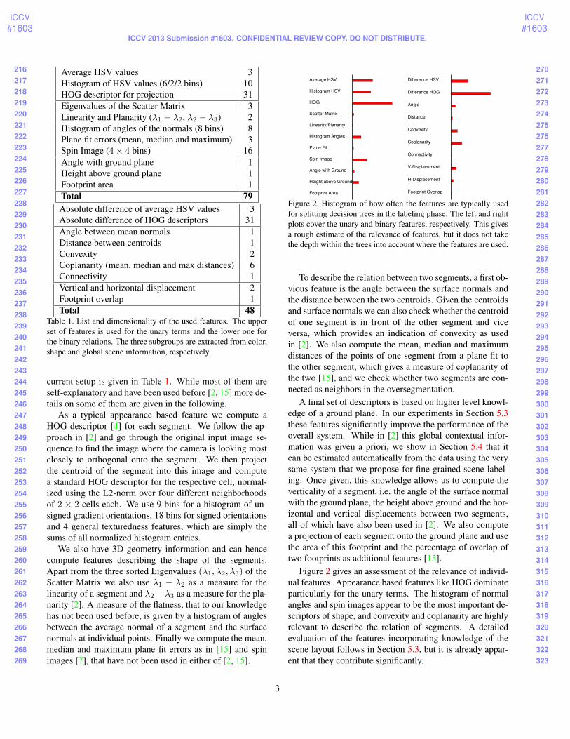
Average HSV values 3Histogram of HSV values (6/2/2 bins) 10HOG descriptor for projection 31Eigenvalues of the Scatter Matrix 3Linearity and Planarity (λ1 − λ2, λ2 − λ3) 2Histogram of angles of the normals (8 bins) 8Plane fit errors (mean, median and maximum) 3Spin Image (4× 4 bins) 16Angle with ground plane 1Height above ground plane 1Footprint area 1Total 79Absolute difference of average HSV values 3Absolute difference of HOG descriptors 31Angle between mean normals 1Distance between centroids 1Convexity 2Coplanarity (mean, median and max distances) 6Connectivity 1Vertical and horizontal displacement 2Footprint overlap 1Total 48

Table 1. List and dimensionality of the used features. The upperset of features is used for the unary terms and the lower one forthe binary relations. The three subgroups are extracted from color,shape and global scene information, respectively.

current setup is given in Table 1. While most of them areself-explanatory and have been used before [2, 15] more de-tails on some of them are given in the following.

As a typical appearance based feature we compute aHOG descriptor [4] for each segment. We follow the ap-proach in [2] and go through the original input image se-quence to find the image where the camera is looking mostclosely to orthogonal onto the segment. We then projectthe centroid of the segment into this image and computea standard HOG descriptor for the respective cell, normal-ized using the L2-norm over four different neighborhoodsof 2 × 2 cells each. We use 9 bins for a histogram of un-signed gradient orientations, 18 bins for signed orientationsand 4 general texturedness features, which are simply thesums of all normalized histogram entries.

We also have 3D geometry information and can hencecompute features describing the shape of the segments.Apart from the three sorted Eigenvalues (λ1, λ2, λ3) of theScatter Matrix we also use λ1 − λ2 as a measure for thelinearity of a segment and λ2−λ3 as a measure for the pla-narity [2]. A measure of the flatness, that to our knowledgehas not been used before, is given by a histogram of anglesbetween the average normal of a segment and the surfacenormals at individual points. Finally we compute the mean,median and maximum plane fit errors as in [15] and spinimages [7], that have not been used in either of [2, 15].

Average HSV

Histogram HSV

HOG

Scatter Matrix

Linearity/Planarity

Histogram Angles

Plane Fit

Spin Image

Angle with Ground

Height above Ground

Footprint Area

Difference HSV

Difference HOG

Angle

Distance

Convexity

Coplanarity

Connectivity

V-Displacement

H-Displacement

Footprint Overlap

Figure 2. Histogram of how often the features are typically usedfor splitting decision trees in the labeling phase. The left and rightplots cover the unary and binary features, respectively. This givesa rough estimate of the relevance of features, but it does not takethe depth within the trees into account where the features are used.

To describe the relation between two segments, a first ob-vious feature is the angle between the surface normals andthe distance between the two centroids. Given the centroidsand surface normals we can also check whether the centroidof one segment is in front of the other segment and viceversa, which provides an indication of convexity as usedin [2]. We also compute the mean, median and maximumdistances of the points of one segment from a plane fit tothe other segment, which gives a measure of coplanarity ofthe two [15], and we check whether two segments are con-nected as neighbors in the oversegmentation.

A final set of descriptors is based on higher level knowl-edge of a ground plane. In our experiments in Section 5.3these features significantly improve the performance of theoverall system. While in [2] this global contextual infor-mation was given a priori, we show in Section 5.4 that itcan be estimated automatically from the data using the verysame system that we propose for fine grained scene label-ing. Once given, this knowledge allows us to compute theverticality of a segment, i.e. the angle of the surface normalwith the ground plane, the height above ground and the hor-izontal and vertical displacements between two segments,all of which have also been used in [2]. We also computea projection of each segment onto the ground plane and usethe area of this footprint and the percentage of overlap oftwo footprints as additional features [15].

Figure 2 gives an assessment of the relevance of individ-ual features. Appearance based features like HOG dominateparticularly for the unary terms. The histogram of normalangles and spin images appear to be the most important de-scriptors of shape, and convexity and coplanarity are highlyrelevant to describe the relation of segments. A detailedevaluation of the features incorporating knowledge of thescene layout follows in Section 5.3, but it is already appar-ent that they contribute significantly.

3

324325326327328329330331332333334335336337338339340341342343344345346347348349350351352353354355356357358359360361362363364365366367368369370371372373374375376377

378379380381382383384385386387388389390391392393394395396397398399400401402403404405406407408409410411412413414415416417418419420421422423424425426427428429430431

ICCV#1603

ICCV#1603


w w

Figure 3. Illustration of the random forest structure in DecisionTree Fields (left), where a table of costs is selected according tothe input data, and Regression Tree Fields (right), where multi-dimensional quadratic cost functions are selected.

4. Semantic LabelingWe model the relation between the collection of feature

vectors x extracted for the nodes and edges and the labelvector y for the scene as a Conditional Random Field. Inour current setup we only consider unary terms EN and bi-nary terms EE , leading to the overall relation:

P (y|x,w) =exp(−E(y,x,w))∫exp(−E(y,x,w))dy

(1)

E(y,x,w) =∑i∈V

EN (yi,x,w) +∑i,j∈N

EE(yi,yj ,x,w)

(2)

with a parameter vector w. Given that we have multipleclasses and the labels for individual nodes in the graph arerelated to each other, this is a classical problem for struc-tured learning and inference techniques. We address it us-ing the two closely related Decision Tree Fields (DTFs) [11]and Regression Tree Fields (RTFs) [6].

For both the DTF and RTF formulations the energiesENand EE are determined using structures akin to RandomForests [3]. As illustrated in Figure 3, the input data x ispassed down a set of trees and eventually selects a singleleaf from each tree. The leaves then determine the energiesrequired to assign the individual labels yi to nodes vi orpairs of labels yi and yj to nodes vi and vj . The definitionof these energies are slightly different for DTFs and RTFs.

For DTFs the labels are discrete yi ∈ [1, . . . ,K], whereK is the number of distinct classes, and the parameter vec-tor w stores tables of energy values for each leaf. The labelyi selects a single entry from the table selected by the inputdata x, and this entry represents the energy for assigningthe label. As there are multiple trees in the forest and hencemultiple leaves, the overall energiesEE andEN are definedas the sums over the energies in the individual leaves:

E(DTF )N (yi,x,w) =

∑q∈L(i,x)

wq,yi (3)

E(DTF )E (yi, yj ,x,w) =

∑q∈L(i,j,x)

wq,yi,yj , (4)

where the functions L(i,x) and L(i, j,x) return the setof leaves reached in the respective forests and wq,yi andwq,yi,yj are the individual energy values.

For RTFs the labels are vectors yi ∈ RK . Each entryof yi encodes the confidence by which the node vi shouldbe labeled as the corresponding class. For the unary termsthe parameter vector w stores a symmetric, positive defi-nite matrix Θu,q ∈ SK and a vector θu,q ∈ RK for eachleaf q, and the energy required to assign a label yi to nodevi is determined by the quadratic energy function definedby Θu,q and θu,q . For the binary terms, the quadratic en-ergy functions stored in the leaves are 2K dimensional anddefined by Θb,q ∈ S2K and θb,q ∈ R2K . They deter-mine the energy required for the concatenated label vectoryi,j = (yTi ,y

Tj )T . The overall energy terms for the ensem-

ble of trees in the forest are again sums over the individualcontributions, resulting in:

E(RTF )N (yi,x,w) =

∑q∈L(i,x)

(1

2yTi Θu,qy − ϑTu,qyi

)(5)

E(RTF )E (yi,yj ,x,w) =

∑q∈L(i,j,x)

(1

2yTi,jΘb,qyi,j − ϑ

Tb,qyi,j

)(6)

These quadratic energy functions can also be interpreted asGaussians with covariance matrices Σ·,q = Θ−1·,q and meanvectors µ·,q = Θ−1·,q θ·,q . In that sense the leaves in theunary regression forests store K-dimensional Gaussian dis-tributions over the label vectors yi, and the binary forestsstore 2K-dimensional distributions over the concatenationsof yi and yj . Accordingly the combined energy E fromequation (2) is a K|V|-dimensional Gaussian, which allowsa very efficient inference step.

Our use of multiple trees appears to be an extension tothe DTFs and RTFs introduced in [11, 6], where only singletrees are used. Multiple trees increase the computationalcomplexity, but also the expressive power of these models,as we show experimentally in Section 5.2.

4.1. Learning

In the learning phase the features x with correspondinglabels y are given as training examples, and we have to findthe model parameters w. As in [11] we determine the treestructures in a first step and then optimize the parameters win a separate, second step. A two step approach is necessaryas the parameters w are continuous whereas the tree struc-tures form a large, combinatorial space, and a simultaneousoptimization of both is intractable.

In the first stage the tree structures are determined us-ing standard methods [3]. We pick a random subset of thetraining data to train each tree in the forest, the binary deci-sion rules at the internal nodes select a random element of

4

432433434435436437438439440441442443444445446447448449450451452453454455456457458459460461462463464465466467468469470471472473474475476477478479480481482483484485

486487488489490491492493494495496497498499500501502503504505506507508509510511512513514515516517518519520521522523524525526527528529530531532533534535536537538539

ICCV#1603

ICCV#1603


the feature vector and split it at a random value. Decisionrules are selected to maximize the information gain and treesplitting is stopped, once a certain depth is reached or theentropy of the remaining labels is below a threshold.

In the second stage of learning we ideally want tomaximize the likelihood from equation (1) w.r.t. w. ForDTFs this involves evaluating the normalization factor∫exp(−E(y,x,w))dy and for RTFs the overall energy

function is of dimension K|V|, both of which are compu-tationally too demanding. Instead a pseudolikelihood ap-proximation of the true likelihood is used [11, 6]:

P (y|x,w) ≈∏i∈V

P (yi|yV\{i},x,w) (7)

Taking the negative log-likelihood we arrive at a non-linearoptimization problem. For DTFs this problem is uncon-strained and can be solved using the standard L-BFGSmethod. For RTFs an additional constraint has to be metwhich enforces that the Θu,q and Θb,q remain positive def-inite matrices. As proposed in [6] we further impose thatthe eigenvalues of Θu,q and Θb,q are constrained to therange [emin, emax] with e.g. emin = 10−4 and emax = 104

to ensure well conditioned matrices throughout. This con-strained optimization problem is solved using a projectedL-BFGS methods based on [14]. In both cases it typicallytakes about 100-200 iterations to find the minimum.

4.2. DTF Inference

In the inference problem we want to find a label vectory for given inputs x and w. For DTFs this is a discrete op-timization problem which is solved using simulated anneal-ing with a Gibbs sampler as proposed in [11]. We define theunnormalized temperized distribution Pτ (y|x,w) as:

Pτ (y|x,w) =∏i∈V

exp(−1

τEN (yi,x,w))

∏i,j∈N

exp(−1

τEE(yi, yj ,x,w)). (8)

Starting from a random initialization y(0) and a high tem-perature coefficient of e.g. τ (0) = 20 we repeatedly samplea new label vector y(t+1) from the above distribution Pτconditioned on the previous y(t) and reduce the temperaturecoefficient by a fixed factor. After typically 100 to 400 iter-ations we arrive at a final temperature of e.g. τ (T ) = 0.01and an approximation y(T ) of the maximum likelihood es-timator of the labels for the given scene.

4.3. RTF Inference

For RTFs an efficient, exact inference method is pre-sented in [6]. Given that all the individual contributions tothe likelihood from Equation (1) are Gaussian, the overall

likelihood is Gaussian as well and the negative log likeli-hood takes the form

− lnP (y|x,w) =1

2yT Θy − ϑ

Ty + lnZ. (9)

For the inference problem we can ignore the normalizationconstant Z and only have to find the mean of the corre-sponding Gaussian, i.e. y = Θ

−1ϑ. Due to the large num-

ber of dimensions an iterative method is required to solvethis linear equation system. Starting from an arbitrary labelvector y(0) = 0 we find y using a standard L-BFGS itera-tion for typically around 10-20 iterations until convergence.

5. Experimental EvaluationWe experimentally evaluate our method primarily us-

ing the Cornell-RGBD-Dataset [2]. Additional results onthe NYU Depth dataset [15] are presented as supplementalmaterial. Both of these contain image sequences recordedwith a Kinect and pose multi-class labeling problems. TheCornell-RGBD-Dataset provides 24 office scenes with 17classes of objects including tables, monitors and printers,and excerpts of this dataset are shown in Figures 1 and 4.Along with the dataset, the authors also provide a set of ex-tracted feature vectors optimized for this task.

In Section 5.1 we show that both Decision Tree Fieldsand Regression Tree Fields have a very competitive perfor-mance compared to state-of-the-art classifiers at much fasterinference times. We then evaluate our extensions in Sec-tion 5.2 showing that a forest of multiple trees increases theperformance of DTFs and RTFs compared to single treesat the expense of higher computational effort. In a third ex-periment in Section 5.3 we evaluate the performance gainedby using global knowledge of a ground plane, and finallywe investigate the performance of the presented methods atfinding such a ground plane in Section 5.4.

5.1. Compared to State-of-the-Art

In [2] a labeling method based on structured SupportVector Machines is presented. This method comes with twodifferent inference algorithms, a slow but accurate one anda much faster, but less accurate one. The authors evaluatedtheir approach by computing macro- and micro-averagedprecision and recall scores on the accompanying Cornell-RGBD-Dataset. Note that the micro-averaged precision andrecall are identical if a label has to be assigned to each of thesegments, but the fast and approximate inference method isallowed to reject segments hence leading to different valuesfor micro-averaged precision and recall.

We evaluate the DTF and RTF classifiers using 5-foldcross validation on the extracted feature vectors comingalong with the dataset and a comparison of the perfor-mances is given in Table 2. The performance of the dif-ferent methods is very similar. If anything, both DTFs and

5

540541542543544545546547548549550551552553554555556557558559560561562563564565566567568569570571572573574575576577578579580581582583584585586587588589590591592593

594595596597598599600601602603604605606607608609610611612613614615616617618619620621622623624625626627628629630631632633634635636637638639640641642643644645646647

ICCV#1603

ICCV#1603


Fine grained labeling Estimating scene layoutRGB Data True labels Predicted labels True labels Predicted labels

Figure 4. Samples of the scene labeling task in the Cornell-RGBD-Dataset. The left column shows the RGB data, the next two columnsshow the ground truth and prediction results for fine grained scene labeling and the right two columns show the same for coarse scenelayout estimation.

Macro P Macro R Micro P Micro R Training Inference

w/o ground plane DTF 70.02 46.11 60.07 10-20sec 50-300msecRTF 65.80 49.65 62.58 1.5-2h 50-300msec

w/ ground plane DTF 85.43 67.63 81.48 10-20sec 50-300msecRTF 85.16 69.65 81.43 3h 50-300msec

w/ ground plane SVM [2] 80.52 72.64 84.06 20-30minSVM approx. [2] 82.95 38.14 87.41 56.82 50msec

Table 2. Experimental evaluation of macro- and micro-averaged precision and recall as well as typical timings for different classificationmethods using the feature vectors extracted in [2].

RTFs have a slightly higher precision than the SVM-basedmethods, RTFs have a slightly higher recall than DTFs, butthe SVM-based method achieves yet a slightly higher recallvalue. However, the inference algorithms for the DTF andRTF methods are orders of magnitudes faster. Altogetherboth DTFs and RTFs achieve roughly the same performanceas the slow but accurate SVM-based inference method inthe same time as the fast but approximate SVM-based in-ference method. This shows that the tree based approachesare highly relevant for the scene labeling task, particularlyif the predicted labels are required at interactive rates.

We also evaluate our overall pipeline of oversegmenta-tion, feature extraction and labeling. Note that the Cornell-RGBD-Dataset only comes with annotated 3D point cloudsand the ground truth labels for these point clouds were origi-nally created by annotating the oversegmentations from [2].For our experiments we therefore try to find suitable groundtruth labels by reprojecting the ground truth point cloud andour oversegmentation into the original camera images andwe reject segments, where the label is not clear.

The results achieved with our proposed pipeline areshown in Table 3, and in this case the RTFs appear to per-form better than DTFs both in labeling performance andinference time. Furthermore, the overall performance isslightly lower compared to the features extracted in [2] and

evaluated in Table 2. As mentioned, the ground truth forthis dataset was obtained by annotating the specific over-segmentations used in [2] and differences in the segmentboundaries will therefore invariably degrade the perfor-mance. The oversegmentation of [2] also results in far lesscomplex CRFs with about 50-100 nodes per scene, whereasour oversegmentations have about 1000-3000 segments ofmuch smaller and much more regular size. This differenceexplains the differences in run time, but on the other handthe samples in Figures 1 and 4 show that the CRF structurein our case strongly encourages contextual consistency forthe many small segments.

5.2. Number of Trees

In Section 4 we proposed to modify the original formu-lations of DTFs and RTFs by using multiple trees instead ofjust a single one per term. With more trees, an increased ac-curacy can be expected at the cost of higher computationalcomplexity. We investigate this effect using the featuresextracted for the Cornell-RGBD-Dataset, and the result-ing macro-averaged precision scores are shown in Figure 5.As expected the performance increases with the number oftrees in both the DTF and RTF formulations and saturateswhen using about 15 trees. Similar, but slightly less pro-nounced increases are also observed for macro-recall and

6

648649650651652653654655656657658659660661662663664665666667668669670671672673674675676677678679680681682683684685686687688689690691692693694695696697698699700701

702703704705706707708709710711712713714715716717718719720721722723724725726727728729730731732733734735736737738739740741742743744745746747748749750751752753754755

ICCV#1603

ICCV#1603


Macro P Macro R Micro P/R Training Inference

w/o ground plane DTF 47.75 18.46 58.06 5-10min 50-120secRTF 60.51 31.68 68.76 10h-12h 15-60sec

w/ ground plane DTF 65.40 39.82 84.43 5-10min 50-120secRTF 69.12 46.74 82.17 10-12h 15-60sec

Table 3. Experimental evaluation of macro- and micro-averaged precision and recall as well as typical timings for DTFs and RTFs usingthe pipeline and feature vectors as explained in this work.

0.6

0.65

0.7

0.75

0.8

0.85

0.9

0 5 10 15 20 25 30

Ma

cro

-Pre

cis

ion

Number of Trees

DTF

RTF

Figure 5. Effect of number of trees on classification performance.

the micro-averaged values, but are omitted for clarity.In this experiment we use the same number of trees for

the unary and binary terms. We have also investigated vary-ing the numbers of trees independently and found that thenumber of binary trees impacts the results more signifi-cantly than the number of unary trees. We attribute thisto the greater diversity in the binary terms, where pairs oflabels have to be predicted instead of a single label per seg-ment. In the remaining experiments, we therefore typicallyuse 10 unary trees and 15 binary trees, which appears tosaturate the performance for most of our tasks.

5.3. Knowledge of Scene Layout

Prior context information such as knowledge of a groundplane and the absolute scale of a scene are important hintsfor the labeling task, and they are thus heavily used in thefeature set we presented in Section 3. To assess their impor-tance we re-run our scene labeling methods without usingthese features and compare the impact. The resulting pre-cision and recall scores are shown in the rows entitled w/oground plane in Tables 2 and 3. The significant drop inprecision and recall scores underlines the relevance of suchglobal knowledge for scene labeling and we next aim to findthis knowledge automatically.

5.4. Estimating Scene Layout

For finding the scene layout we try to infer one of thelabels {floor, wall, tableTop, clutter} for each of the seg-ments in the scene, and achieve this using the very samescene labeling approach as before. We reduce the set of la-bels to the given four classes and re-run the training and in-ference steps. Sample results of this labeling task are shown

0

10

20

30

40

50

60

70

80

90

0 0.1 0.2 0.3 0.4 0.5 0.6 0.7 0.8 0.9 1

Gro

un

d p

lan

e e

stim

atio

n e

rro

r [d

eg

ree

]

Percentage of experiments

DTFRTF

Figure 6. Errors in the estimation of the ground plane normal.

Macro P Macro R Micro P/R Training InferenceDTF 73.94 44.10 59.27 10-20min 30-100secRTF 74.65 61.16 68.93 30-40min 5-20sec

Table 4. Experimental evaluation of precision and recall for esti-mating the coarse scene layout using DTFs and RTFs.

on the right hand side of Figure 4. To evaluate the perfor-mance we again compute the precision and recall values asa first evaluation criterion. As a second criterion we alsocompute a robust plane fit to the segments labeled as floorby our system and in the ground-truth data and compute theangle between the two recovered normals.

In Table 4 we present the labeling precision and recallthus achieved with our system. While this metric gives afirst impression of the performance, a much more relevantcriterion is the final estimation of the ground plane that isachieved with our method, and a quantile-plot of the an-gular errors is given in Figure 6. From both evaluations itappears that RTFs perform better in this task than DTFs andthe proposed method estimates the ground plane to within20◦ in 80% of the cases. For an overall system it is straightforward to apply a two stage approach. In the first step, thecoarse prediction is used to estimate the ground plane, andin the second step, this ground plane is used in the compu-tation of a fine grained scene labeling. While this can beexpected to fail in a few cases, it eliminates the need forprior knowledge about the camera setup.

6. ConclusionsWe have introduced a structured learning approach to 3D

scene labeling that takes advantage of the recently describedDecision Tree Field [11] and Regression Tree Field [6] clas-

7

756757758759760761762763764765766767768769770771772773774775776777778779780781782783784785786787788789790791792793794795796797798799800801802803804805806807808809

810811812813814815816817818819820821822823824825826827828829830831832833834835836837838839840841842843844845846847848849850851852853854855856857858859860861862863

ICCV#1603

ICCV#1603


sifiers within a Conditional Random Field framework. Weshow that both DTFs and RTFs achieve an almost identical,if not superior, prediction accuracy to state-of-the-art SVM-based methods, but allow for much more efficient inferencesteps. The input to our method are volumetric representa-tions of the 3D scene, which are efficiently computed usingKinectFusion [10], and at the same time the dense repre-sentation of the 3D data is very well suited to compute theoversegmentation and the features required for scene label-ing. Overall we have shown that prediction accuracy, andparticularly the fast inference times of this new method areclearly important for the scene labeling problem. Besidesthe detailed semantic labeling of 3D scenes, another impor-tant application of the presented method is a coarse labelinginto structures like the floor and walls of indoor environ-ments. This information then provides valuable additionalfeatures like the height above ground, which are crucial forthe performance of fine grained scene labeling systems.

There are a number of practical measures that could betaken to improve the system. Our oversegmentation stepfrom Section 2 computes a dense set of many, small seg-ments. While this allows a fine grained segmentation ofobject boundaries and while the CRF formulation does anexcellent job at grouping these small segments into semanti-cally consistent units, the sheer number of segments poses ahigh computational burden on the CRF. It would be interest-ing to improve upon this by e.g. pre-grouping very similarsegments or even using hierarchical approaches. Also wecurrently impose an empirical threshold on the connectivityof the CRF in an attempt to manage the computational com-plexity by limiting the context range. Although this worksquite well, and certainly is much more flexible than tradi-tional 4- or 8-connected MRF/CRF models, long range in-teractions that may be important such as the relationship be-tween bounding walls may not be modeled because of thecutoff. Again, a hierarchical approach with long-range con-textual relations between objects and short range relationsbetween individual parts of the objects might be beneficial.Finally our current system currently relies on a Kinect sen-sor and the KinectFusion system, but volumetric 3D scenerepresentations can recently also be acquired with standardRGB cameras and DTAM [9]. While we expect the 3Dshape information to be less reliable in this case, it wouldbe interesting to compare the performance.

References

[1] R. Achanta, A. Shaji, K. Smith, A. Lucchi, P. Fua, andS. Susstrunk. Slic superpixels compared to state-of-the-artsuperpixel methods. IEEE Transactions on Pattern Analysisand Machine Intelligence, 34(11):2274–2282, Nov. 2012. 2

[2] A. Anand, H. S. Koppula, T. Joachims, and A. Saxena.Contextually guided semantic labeling and search for three-

dimensional point clouds. The International Journal ofRobotics Research, 32(1):19–34, 2013. 1, 2, 3, 5, 6

[3] L. Breiman. Random forests. Machine Learning, 45(1):5–32, 2001. 1, 4

[4] N. Dalal and B. Triggs. Histograms of oriented gradients forhuman detection. In IEEE Conference on Computer Visionand Pattern Recognition, volume 1, pages 886–893, 2005. 3

[5] A. Flint, D. Murray, and I. Reid. Manhattan scene under-standing using monocular, stereo, and 3d features. In IEEEInternational Conference on Computer Vision (ICCV), pages2228–2235. IEEE, 2011. 2

[6] J. Jancsary, S. Nowozin, and C. Rother. Regression treefields an efficient, non-parametric approach to image label-ing problems. In 25th IEEE Conference on Computer Visionand Pattern Recognition (CVPR), pages 2376–2383, 2012.1, 2, 4, 5, 7

[7] A. Johnson and M. Hebert. Using spin images for efficientobject recognition in cluttered 3d scenes. IEEE Transactionson Pattern Analysis and Machine Intelligence, 21(5):433–449, May 1999. 3

[8] G. Klein and D. Murray. Parallel tracking and mapping on acamera phone. In Proc. Eigth IEEE and ACM InternationalSymposium on Mixed and Augmented Reality (ISMAR’09),pages 83–86, Oct. 2009. 1

[9] R. Newcombe, S. Lovegrove, and A. Davison. Dtam: Densetracking and mapping in real-time. In IEEE InternationalConference on Computer Vision (ICCV), pages 2320–2327,Nov. 2011. 1, 8

[10] R. A. Newcombe, S. Izadi, O. Hilliges, D. Molyneaux,D. Kim, A. J. Davison, P. Kohli, J. Shotton, S. Hodges, andA. Fitzgibbon. Kinectfusion: Real-time dense surface map-ping and tracking. In Proceedings of the 2011 10th IEEEInternational Symposium on Mixed and Augmented Reality,pages 127–136, 2011. 1, 2, 8

[11] S. Nowozin, C. Rother, S. Bagon, T. Sharp, B. Yao, andP. Kohli. Decision tree fields. In IEEE International Con-ference on Computer Vision (ICCV), pages 1668–1675, Nov.2011. 1, 2, 4, 5, 7

[12] I. Posner, M. Cummins, and P. Newman. A generative frame-work for fast urban labeling using spatial and temporal con-text. Autonomous Robots, 26(2):153–170, 2009. 1

[13] X. Ren, L. Bo, and D. Fox. Rgb-(d) scene labeling: Featuresand algorithms. In IEEE Conference on Computer Visionand Pattern Recognition (CVPR), pages 2759–2766, 2012. 1

[14] M. Schmidt, E. Van Den Berg, M. Friedlander, and K. Mur-phy. Optimizing costly functions with simple constraints: Alimited-memory projected quasi-newton algorithm. In Proc.of Conf. on Artificial Intelligence and Statistics, pages 456–463, 2009. 5

[15] N. Silberman and R. Fergus. Indoor scene segmentation us-ing a structured light sensor. In IEEE International Con-ference on Computer Vision Workshops (ICCV Workshops),pages 601–608, Nov. 2011. 1, 2, 3, 5

[16] H. Wang, S. Gould, and D. Koller. Discriminative learn-ing with latent variables for cluttered indoor scene under-standing. In IEEE European Conference on Computer Vision(ECCV), pages 435–449. Springer, 2010. 2

8

efficient 3d scene labeling using fields of trees - robotics

Documents