efficient analysis, design and decoding of low-density
TRANSCRIPT

Efficient Analysis, Design and Decoding of
Low-Density Parity-Check Codes
by
Masoud Ardakani
A thesis submitted in conformity with the requirementsfor the Degree of Doctor of Philosophy,The Edward S. Rogers Sr. Departmentof Electrical and Computer Engineering,
University of Toronto
c© Copyright by M. Ardakani, 2004

Efficient Analysis, Design and Decoding of Low-Density
Parity-Check Codes
Masoud Ardakani
Doctor of Philosophy
The Edward S. Rogers Sr. Department of Electrical and Computer Engineering
University of Toronto
2004
Abstract
This dissertation presents new methods for the analysis, design and decoding of low-
density parity-check (LDPC) codes. We start by studying the simplest class of decoders:
the binary message-passing (BMP) decoders. We show that the optimum BMP decoder
must satisfy certain symmetry and isotropy conditions, and prove that Gallager’s Algorithm
B is the optimum BMP algorithm. We use a generalization of extrinsic information transfer
(EXIT) charts to formulate a linear program that leads to the design of highly efficient irreg-
ular LDPC codes for the BMP decoder. We extend this approach to the design of irregular
LDPC codes for the additive white Gaussian noise channel. We introduce a “semi-Gaussian”
approximation that very accurately predicts the behaviour of the decoder and permits code
design over a wider range of rates and code parameters than in previous approaches. We
then study the EXIT chart properties of the highest rate LDPC code which guarantees a
certain convergence behaviour. We also introduce and analyze gear-shift decoding in which
the decoder is permitted to select the decoding rule from among a predefined set. We show
that this flexibility can give rise to significant reductions in decoding complexity. Finally, we
show that binary LDPC codes can be combined with quadrature amplitude modulation to
achieve near-capacity performance in a multitone system over frequency selective Gaussian
channels.
i

Acknowledgements
This work would not be possible without the valuable support, advice and comments of my
supervisor Prof. Frank Kschischang. Frank contributed endless hours of advice and guidance
regarding conducting research, writing papers, presentation skills, and more importantly life
in general. I could not imagine an adviser more caring, encouraging and supportive who was
willing to help in all aspects of my work.
I wish to thank Frank for many things: his insights and ideas are infused throughout
this work; his tireless editorial effort has vastly improved the quality of this dissertation
(and of much of the rest of my research); his admirable personality made my Ph.D. studies
a wonderful journey for me; and the list goes on and on. The best thing about having a
supervisor as smart as Frank is that in every occasion he finds you a very elegant fundamental
problem. Such an elegant problem, that you cannot resist trying it. The bad thing is that
you feel being vastly outsmarted every day!
I also wish to thank the members of the evaluation committee: Prof. Ian F. Blake,
Prof. Pas S. Pasupathy, Prof. Bruce A. Francis, Prof. Wei Yu, Prof. Konstantinos N. Pla-
taniotis and Prof. William E. Ryan of the University of Arizona for their effort, discussions
and advice which helped me a lot in improving this thesis.
I wish to thank all my friends from the Communications Group: Steve Hranilovic,
Mehrdad Shamsi, Tooraj Esmailian, Terence Chan, Sujit Sen, Ivo Maljevic, Stark Draper,
Aaron Meyers, Andrew Eckford, Yongyi Mao, Guang-Chong Zhu, Christina Park, Vladimir
Pechenkin, ... for all the fruitful discussions that we had on the topic of my thesis or any
other subject. I feel lucky to have so many brilliant, endowed colleagues from whom I learned
more than I could imagine beforehand. I wish that our friendship will continue beyond our
professional lives.
I am grateful to the University of Toronto, the Government of Ontario and Ted and
Loretta Rogers for their direct financial support of my work in the form of scholarships and
awards.
I would like to acknowledge everybody back home, my family and my friends, who did
not forget me even though I left them to study thousands of miles away from them.
Last but not least, my special thanks goes to Helia Koosha, my loving wife, who enriched
my whole life and this work as a part of it. I am truly unable to thank Helia for her support
and help in the process of completion of this work.
ii

Contents
Abstract i
List of Figures vi
1 Introduction 1
1.1 Codes Defined on Graphs . . . . . . . . . . . . . . . . . . . . . . . . . . . . 11.2 A Brief History of Graphical Codes . . . . . . . . . . . . . . . . . . . . . . . 21.3 Overview of The Thesis . . . . . . . . . . . . . . . . . . . . . . . . . . . . . 5
1.3.1 The Main Theme of This Work . . . . . . . . . . . . . . . . . . . . . 61.3.2 Organization of the Thesis . . . . . . . . . . . . . . . . . . . . . . . . 8
2 LDPC Codes and Their Analysis 10
2.1 Graphical Models and Message-Passing Decoding . . . . . . . . . . . . . . . 102.2 LDPC codes: Structure . . . . . . . . . . . . . . . . . . . . . . . . . . . . . . 122.3 LDPC codes: Decoding . . . . . . . . . . . . . . . . . . . . . . . . . . . . . . 15
2.3.1 The sum-product algorithm . . . . . . . . . . . . . . . . . . . . . . . 162.3.2 An interpretation of the sum-product algorithm . . . . . . . . . . . . 182.3.3 Other decoding algorithms . . . . . . . . . . . . . . . . . . . . . . . . 19
2.4 LDPC codes: Analysis . . . . . . . . . . . . . . . . . . . . . . . . . . . . . . 212.4.1 Gallager’s analysis of LDPC codes . . . . . . . . . . . . . . . . . . . . 222.4.2 The decoding tree . . . . . . . . . . . . . . . . . . . . . . . . . . . . . 232.4.3 Density evolution for LDPC codes . . . . . . . . . . . . . . . . . . . . 242.4.4 Decoding threshold of an LDPC code . . . . . . . . . . . . . . . . . . 262.4.5 Extrinsic information transfer chart analysis . . . . . . . . . . . . . . 26
3 Binary Message-Passing Decoding of LDPC Codes 29
3.1 Assumptions and definitions . . . . . . . . . . . . . . . . . . . . . . . . . . . 303.2 Necessity of Symmetry and Isotropy Conditions . . . . . . . . . . . . . . . . 333.3 Optimality of Algorithm B for Regular Codes . . . . . . . . . . . . . . . . . 403.4 Irregular Codes . . . . . . . . . . . . . . . . . . . . . . . . . . . . . . . . . . 45
3.4.1 Stability condition . . . . . . . . . . . . . . . . . . . . . . . . . . . . 513.4.2 Low error-rate channels . . . . . . . . . . . . . . . . . . . . . . . . . 52
3.5 Conclusions . . . . . . . . . . . . . . . . . . . . . . . . . . . . . . . . . . . . 54
iii

4 A More Accurate One-Dimensional Analysis and Design of Irregular LDPC
Codes 56
4.1 Gaussian Assumption on Messages . . . . . . . . . . . . . . . . . . . . . . . 584.1.1 Semi-Gaussian vs. All-Gaussian Approximation . . . . . . . . . . . . 594.1.2 EXIT charts based on different measures . . . . . . . . . . . . . . . . 644.1.3 The choice of parameter for analysis . . . . . . . . . . . . . . . . . . 66
4.2 Analysis of Regular LDPC Codes . . . . . . . . . . . . . . . . . . . . . . . . 674.3 Analysis of Irregular LDPC Codes . . . . . . . . . . . . . . . . . . . . . . . . 714.4 Design of Irregular LDPC Codes . . . . . . . . . . . . . . . . . . . . . . . . . 754.5 Examples and Numerical Results . . . . . . . . . . . . . . . . . . . . . . . . 784.6 Conclusions . . . . . . . . . . . . . . . . . . . . . . . . . . . . . . . . . . . . 83
5 EXIT-Chart Properties of the Highest-Rate LDPC Code with Desired
Convergence Behaviour 85
5.1 Background and Problem Definition . . . . . . . . . . . . . . . . . . . . . . . 865.2 Problem Formulation . . . . . . . . . . . . . . . . . . . . . . . . . . . . . . . 86
5.2.1 Desired convergence behaviour . . . . . . . . . . . . . . . . . . . . . . 885.2.2 Monotonic Decoders . . . . . . . . . . . . . . . . . . . . . . . . . . . 89
5.3 Results . . . . . . . . . . . . . . . . . . . . . . . . . . . . . . . . . . . . . . . 895.4 Discussion and Examples . . . . . . . . . . . . . . . . . . . . . . . . . . . . . 92
6 Near-Capacity Coding in Multi-Carrier Modulation Systems 95
6.1 Background . . . . . . . . . . . . . . . . . . . . . . . . . . . . . . . . . . . . 976.1.1 Our approach . . . . . . . . . . . . . . . . . . . . . . . . . . . . . . . 976.1.2 Multilevel coding . . . . . . . . . . . . . . . . . . . . . . . . . . . . . 99
6.2 Channel Model . . . . . . . . . . . . . . . . . . . . . . . . . . . . . . . . . . 1016.3 System Structure . . . . . . . . . . . . . . . . . . . . . . . . . . . . . . . . . 1026.4 System specifications . . . . . . . . . . . . . . . . . . . . . . . . . . . . . . . 107
6.4.1 Bit-loading algorithm . . . . . . . . . . . . . . . . . . . . . . . . . . . 1096.4.2 System Complexity . . . . . . . . . . . . . . . . . . . . . . . . . . . . 111
6.5 Simulation Results . . . . . . . . . . . . . . . . . . . . . . . . . . . . . . . . 1126.6 Conclusion . . . . . . . . . . . . . . . . . . . . . . . . . . . . . . . . . . . . . 115
7 Gear-Shift Decoding 117
7.1 Gear-shift decoding . . . . . . . . . . . . . . . . . . . . . . . . . . . . . . . . 1197.1.1 Definitions and assumptions . . . . . . . . . . . . . . . . . . . . . . . 1207.1.2 Equally-complex algorithms . . . . . . . . . . . . . . . . . . . . . . . 1207.1.3 Algorithms with varying complexity . . . . . . . . . . . . . . . . . . . 1237.1.4 Convergence threshold of the gear-shift decoder . . . . . . . . . . . . 125
7.2 Minimum Hardware Decoding . . . . . . . . . . . . . . . . . . . . . . . . . . 1267.3 Examples . . . . . . . . . . . . . . . . . . . . . . . . . . . . . . . . . . . . . 1287.4 Conclusion . . . . . . . . . . . . . . . . . . . . . . . . . . . . . . . . . . . . . 134
iv

8 Conclusion 136
8.1 Summary of Contributions . . . . . . . . . . . . . . . . . . . . . . . . . . . . 1368.2 Possible Future Work . . . . . . . . . . . . . . . . . . . . . . . . . . . . . . . 137
A Sum-Product Algorithm 139
B Discrete Density Evolution 142
C Analysis of Algorithm A 144
D Table of Notation 146
v

List of Figures
1.1 Illustrative performance of turbo codes and convolutional codes. . . . . . . . . . 31.2 Comparison between performance of rate 1/2 LDPC code of different length with
turbo code of the same length. . . . . . . . . . . . . . . . . . . . . . . . . . . 7
2.1 The factor graph representing the factorization of Equation (2.1). . . . . . . . . 112.2 A bipartite graph representing a parity-check code. . . . . . . . . . . . . . . . . 122.3 Intrinsic and extrinsic messages at the variable node x1. Also, the incoming
messages that effect an outgoing message at the check node c3. . . . . . . . . 182.4 The principle of iterative decoding. . . . . . . . . . . . . . . . . . . . . . . . . 222.5 The depth-one decoding tree for a regular (3, 6) LDPC code. . . . . . . . . . . 232.6 A depth-two decoding tree for an irregular LDPC code. . . . . . . . . . . . . . 242.7 An EXIT chart based on message error rate. . . . . . . . . . . . . . . . . . . . 27
3.1 Messages at a check node. . . . . . . . . . . . . . . . . . . . . . . . . . . . . . 353.2 Messages at a variable node. . . . . . . . . . . . . . . . . . . . . . . . . . . . . 363.3 EXIT charts for different decoding algorithms in the case of a regular (6,10) code. 453.4 EXIT charts for various dv, fixing dc = 10. . . . . . . . . . . . . . . . . . . . . 48
4.1 The output density of a degree six check node, fed with symmetric Gaussiandensity of −1dB, is compared with the symmetric Gaussian density of the samemean. . . . . . . . . . . . . . . . . . . . . . . . . . . . . . . . . . . . . . . . 60
4.2 The output density of a degree six check node, fed with symmetric Gaussiandensity of 5dB, is compared with the symmetric Gaussian density of the same mean. 61
4.3 The output density of a degree 10 check node, fed with symmetric Gaussiandensity of 5dB, is compared with the symmetric Gaussian density of the same mean. 62
4.4 The output density of a degree six variable node, fed with the output density ofFig. 4.1, is compared with the symmetric Gaussian density of the same mean. . . 63
4.5 A depth-one tree for a (3, 6) regular LDPC code . . . . . . . . . . . . . . . . . 644.6 EXIT chart, based on single iteration analysis, comparing the predicted and actual
decoding trajectories for a regular (3, 6) code of length 200,000. . . . . . . . . . 684.7 Compares the actual results for a regular (3, 6) code of length 200,000 with
predicted trajectory based on single iteration analysis. . . . . . . . . . . . . . . 694.8 Compares the actual results for regular (3, 6) code of length 5,000 and 1,000 with
the predicted trajectory. . . . . . . . . . . . . . . . . . . . . . . . . . . . . . . 704.9 Shows the input and output densities for a degree 6 check node when the input
is single Gaussian and when it is a mixture of two Gaussians. . . . . . . . . . . . 73
vi

4.10 EXIT charts for different variable degrees on AWGN channel at −1.91dB whendc = 6. . . . . . . . . . . . . . . . . . . . . . . . . . . . . . . . . . . . . . . . 75
4.11 Actual convergence behaviour of an irregular code compared with the predictedtrajectory using the semi-Gaussian and the all-Gaussian methods. . . . . . . . . 76
4.12 Illustrates the improved accuracy of elementary exit charts when a Gaussian mix-ture assumption is made on the messages. . . . . . . . . . . . . . . . . . . . . 79
4.13 Shows elementary EXIT charts for different variable degrees on AWGN channel at−1.91dB when dc = 8. . . . . . . . . . . . . . . . . . . . . . . . . . . . . . . . 80
4.14 Shows elementary EXIT charts for different variable degrees on AWGN channel at−1.91dB when dc = 7. . . . . . . . . . . . . . . . . . . . . . . . . . . . . . . . 81
5.1 Comparison of EXIT charts for two irregular codes. . . . . . . . . . . . . . . . . 875.2 Comparison of EXIT charts for two irregular codes, which are designed with dif-
ferent desired convergence behaviour curves. . . . . . . . . . . . . . . . . . . . 94
6.1 Net capacity and capacities associated with bit-channels (bit-channel 0: I(Y ; b0),bit-channel 1: I(Y ; b1|b0), bit-channel 2: I(Y ; b2|b0, b1)) for 4-QAM/8-QAM sig-nalling when an Ungerboeck-labelling is used. . . . . . . . . . . . . . . . . . . 101
6.2 General structure of a multilevel encoder. . . . . . . . . . . . . . . . . . . . . . 1026.3 General structure of a multilevel decoder. . . . . . . . . . . . . . . . . . . . . . 1036.4 The magnitude of the frequency response of three test channels (same as Fig.
6.11 of [52]). . . . . . . . . . . . . . . . . . . . . . . . . . . . . . . . . . . . . 1046.5 Labelling of a 16-QAM constellation in our system. . . . . . . . . . . . . . . . 1056.6 The block diagram of the encoder of the proposed system. . . . . . . . . . . . . 1066.7 The block diagram of the decoder of the proposed system. . . . . . . . . . . . . 1076.8 Shows Cb0b1 , bit-channel capacity for b2 and the PDF of sub-channels as a function
of SNR. . . . . . . . . . . . . . . . . . . . . . . . . . . . . . . . . . . . . . . 116
7.1 Compares the convergence behaviour of two different binary message passing al-gorithm. . . . . . . . . . . . . . . . . . . . . . . . . . . . . . . . . . . . . . . 122
7.2 A simple trellis of decoding performance with P of size 6 and 3 algorithms. Noticethat some of the states have fewer than 3 outgoing edges. This happens whensome algorithms have a closed EXIT chart at this message error rate. . . . . . . 124
7.3 A proposed pipeline decoder for high-throughput systems. . . . . . . . . . . . . 1277.4 Shows the EXIT charts for a (3 6) LDPC code under different decoding algorithms
when the channel is Gaussian with SNR=1.75 dB. . . . . . . . . . . . . . . . . 131
C.1 Four decoding scenarios for a regular (5, 10) LDPC code under Algorithm A: (a)A case of decoding failure. The EXIT chart is closed at a message error rate ofabout 0.02. (b) Another case of failure. (c) Decoding at the threshold. The EXITchart is about to close. (d) A case of successful decoding. The EXIT chart is open.145
vii

Science may be described as the art of systematic over-simplification.Karl Popper 1902-1994
viii

To my parents and my wife.
ix

Chapter 1
Introduction
This work is concerned with the analysis, design and decoding of an extremely powerful and
flexible family of error-control codes called low-density parity-check (LDPC) codes. LDPC
codes can be designed to perform close to the capacity of many different types of channels
with a practical decoding complexity. It is conjectured that they can achieve the capacity
of many channels and, indeed, they have been shown to achieve the capacity of the binary
erasure (BEC) channel, under iterative decoding.
This chapter introduces some of the concepts which are explored in this thesis. We will
discuss the importance of the field of study, the interesting problems that have attracted
researchers to this area and some of the open problems. We will discuss the problems that
we have tackled and provide an overview of the thesis.
1.1 Codes Defined on Graphs
Since 1948, when Claude Shannon introduced the notion of channel capacity [1], the ultimate
goal of coding theory has been to find practical capacity-approaching codes. According to
Shannon’s channel capacity theorem, reliable communication at a rate R (bits/channel-use)
over an additive white Gaussian noise (AWGN) channel requires a certain minimum signal-
to-noise ratio, called the Shannon limit. In terms of the normalized ratio Eb/N0 of bit energy
1

Chapter 1: Introduction 2
to noise density, reliable communication can take place at rate R provided
Eb
N0
≥ 22R − 1
2R,
where Eb is the average energy per transmitted bit and N0/2 is the variance of the channel’s
zero mean Gaussian noise. The minimum required Eb/N0 is referred to as the Shannon limit.
Approaching the Shannon limit within a few decibels (dBs) was possible with practical
decoding complexity, by using convolutional codes, but reducing this gap required imprac-
tical complexity until the discovery of turbo codes [2]. One of the important innovations
in turbo codes was the introduction of a class of low-complexity suboptimal decoding rules,
i.e., iterative message-passing algorithms. Using an iterative message-passing decoder, turbo
codes provide excellent performance and a small gap to the Shannon limit with a low (prac-
tical) decoding complexity. Fig. 1.1 compares the typical performance of a turbo code and
a convolutional code on an AWGN channel (see [3, Fig. 5 ] for example). This amazing
performance of turbo codes drew a lot of attention to the field of study, which soon extended
to a more general class of codes called codes defined on graphs.
Codes defined on graphs can be decoded with message-passing algorithms. The two
important features of message-passing decoding which make codes defined on graphs so
attractive, are its (potentially) very close to optimal performance and its practical complexity
which (for a fixed number of iterations) increases linearly with the length of the code. This,
in turn, allows for the use of very long codes. Therefore, about 50 years after Shannon’s
work, coding specialists are now able to find codes which can perform close to the Shannon
limit with a reasonable decoding complexity. Moreover, for some channels, they have learned
how the capacity can be achieved in principle, although the decoder requires an increasing
complexity as the code’s performance approaches capacity.
1.2 A Brief History of Graphical Codes
Interestingly, it was after the discovery of some of the later-called graphical codes that a
graphical understanding of them formed. Not only has this understanding helped coding
theorists in analysis of these codes and design of decoding algorithms for them, they also

Chapter 1: Introduction 3
0 2 4 6 8 10 1210
−7
10−6
10−5
10−4
10−3
10−2
10−1
Eb/N
0 (dB)
Bit
Err
or R
ate
UncodedConvolutional CodeTurbo code
Shannon Lim
it
Figure 1.1: Illustrative performance of turbo codes and convolutional codes.
learned how to design their codes to get the best out of a given decoding algorithm.
The graphical understanding of codes started with Tanner graphs for linear codes [4].
Later, Wiberg uncovered that the turbo decoder can also be represented graphically [5].
Soon after this discovery, both in [6] and in [7], it was shown that turbo decoding algorithm
on the graphical representation of a turbo code is a special case of belief propagation on
general Bayesian networks [8].
Parallel to the research on turbo codes and influenced by the focus on turbo codes, in
1996 MacKay and Neal in [9] and Sipser and Spielman in [10] rediscovered a long forgotten
class of codes, i.e., LDPC codes. This class of codes was originally proposed in 1962 by
Gallager [11], but were considered too complex at the time of their discovery.
LDPC codes drew a lot of attention to themselves as they had an extremely good per-
formance. For example, on the AWGN channel they can be designed to perform a few
hundredths of a dB away from the Shannon limit. Another feature of LDPC codes is their
simple graphical representation, which is based on Tanner’s representation of linear codes [4].

Chapter 1: Introduction 4
This simple structure allows for accurate asymptotic analysis of LDPC codes [12,13] as well
as design of good irregular LDPC codes, optimized under specific constraints.
Since the rediscovery of LDPC codes, there has been a lot of research activity and im-
provements in the area of codes defined on graphs. Undoubtedly, research on LDPC codes
has played and will continue to play a central role in this field, as many of the new classes of
codes which are defined on graphs are influenced by the structure of LDPC codes. Examples
include repeat-accumulate (RA) codes [14], Luby transform codes [15] and concatenated tree
codes [16]. Some of the key improvements in the field of graphical codes and their importance
are highlighted below.
• Irregular LDPC codes: As shown in [17], irregular LDPC codes can significantly out-
perform regular LDPC codes. All LDPC codes which can approach the Shannon limit
on different channels are irregular LDPC codes. The discovery of irregular LDPC codes
influenced consideration of irregular structures for other codes defined on graphs such
as irregular turbo codes [18] and irregular RA codes [19].
• Repeat-accumulate codes: One issue with LDPC codes is their encoding complexity.
People have considered different ways of adding structure to LDPC codes to make
the encoding process less complex. One of the best solutions is RA codes [14], which
have a slightly different structure than LDPC codes and suffer minor performance loss
compared to LDPC codes. The encoding complexity of RA codes grows linearly with
the block length.
• Capacity achieving LDPC codes for the BEC: Shokrollahi found a family of irregular
LDPC codes that could achieve the capacity of the BEC [20,21].
• Density evolution analysis of LDPC codes: An accurate asymptotic analysis of LDPC
codes under different decoding schemes became possible [13]. The idea is to follow the
evolution of the density of the messages in the decoder. Using this analysis, design
of good irregular LDPC codes, which has already been studied for the BEC became
possible for other channel types.

Chapter 1: Introduction 5
• Gaussian analysis of turbo codes and LDPC codes [22–24]: Due to computational
complexity of density evolution, approximations of density evolution attracted many
researchers. In particular, approximating the true message density with a Gaussian
density seemed to be very effective.
• Extrinsic Information Transfer (EXIT) chart analysis: EXIT chart analysis [25] is
similar to density evolution, except that it follows the evolution of a single parameter
that represents the density of messages. This evolution can be visualized in a graph
called an EXIT chart. EXIT charts have become very popular, as they provide deep
insight to the behaviour of iterative decoders.
• Luby Transform (LT) codes [15]: The idea of rateless codes is one of the latest inven-
tions in the field of coding theory. Such codes are useful when we have a broadcasting
transmitter, whose channel to each receiver is different from another. In such cases, it
is not clear what code rate should be used for data protection. LT codes are rateless
codes which solve this problem. To be more specific, each receiver gets a different data
rate depending on its channel condition.
The research in the area of graphical codes is still very active and there are many open
problems under study.
1.3 Overview of The Thesis
LDPC codes are one of the most important codes defined on graphs. This is due to their
excellent performance as well as their simple yet flexible structure. As mentioned above,
many codes defined on graphs have been influenced by the structure of LDPC codes. This
makes research on LDPC codes central to the field.
LDPC codes are already used in some standards such as ETSI EN 302 307 for digital
video broadcasting [26] and IEEE 802.16 (Broadband Wireless Access Working Group) for
coding on orthogonal frequency division multiplexing access (OFDMA) systems [27].
There are still many open problems in the area of LDPC coding. This thesis has addressed
some of these problems and has opened a number of new problems.

Chapter 1: Introduction 6
1.3.1 The Main Theme of This Work
This thesis describes the effective methods for the design and analysis of low-density parity-
check (LDPC) codes and their decoders. These problems are studied from a practical point of
view and a number of interesting questions are raised. Some of these questions are answered
in this work and some are left as open problems. In brief, this thesis addresses three main
problems:
• effective methods for the analysis of LDPC codes;
• effective methods for the design of irregular LDPC codes;
• improved decoding strategies for LDPC codes.
Although the emphasis is on LDPC codes, some of these problems are discussed beyond
their application to LDPC codes. In this section, we review the general organization of the
thesis, and provide a summary of the major results.
Fig. 1.2 compares typical performance of irregular LDPC codes of length 104 and 105
with turbo codes of equal length on the AWGN channel. Turbo codes can outperform LDPC
codes at short blocklengths, but it can be seen from Fig. 1.2 that when the blocklength is
large (typically more than 5000), irregular LDPC codes can outperform turbo codes of equal
length. As the code length increases the performance improves. An LDPC code of length
106 can be decoded reliably at an Eb/N0 less than 0.1 dB away from the Shannon limit on
the AWGN channel and with a blocklength of 107 the gap to the Shannon limit can be closed
to less than 0.04 dB [28].
This amazing performance is achieved through careful design of the irregularity of the
code. Unfortunately, except for a few cases, these design procedures can be very computa-
tionally intensive. The conventional design method is to set some irregularity in the code,
check the performance with density evolution, and vary the irregularity in the code until the
desired performance is achieved. One interesting problem that is addressed in the literature
is to simplify the design procedure of LDPC codes [24]. This will be a major focus of this
work.

Chapter 1: Introduction 7
0 0.5 1 1.5 210
−7
10−6
10−5
10−4
10−3
10−2
turbo code n=104
LDPC code n=104
turbo code n=105
LDPC code n=105
Shannon Lim
it
Eb/N
0 (dB)
Bit
Err
or R
ate
Figure 1.2: Comparison between performance of rate 1/2 LDPC code of different length with
turbo code of the same length.
Construction of less complex decoding algorithms is another goal of researchers in the
area. We will address this important problem in this work and will show that, using the
existing algorithms, less complex decoding is possible simply by allowing the decoder to
choose its decoding rule among a set of predefined rules. We call this technique gear-shift
decoding as the decoder shifts gears (changes it decoding rule) in order to speed up the
decoding.
Another fundamental open problem is the best performance that can be achieved for
a certain amount of complexity. We study this problem in a special case, where a certain
convergence behaviour is desired. We find some of the properties of the highest rate LDPC
code which guarantees the desired convergence behaviour.
We also consider some practical problems, such as application of LDPC codes in frequency-
selective channels. We show that LDPC codes have some attributes that make them a nice
solution for coding on such channels.

Chapter 1: Introduction 8
1.3.2 Organization of the Thesis
In Chapter 2 we provide the necessary background on LDPC codes, their decoding algorithms
and the existing analysis methods for these decoding algorithms.
In Chapter 3, we study LDPC decoding using binary message-passing algorithms. We
track the message error rate to analyze the decoder and provide EXIT charts based on
message error rate for that purpose. We also prove that Gallager’s Algorithm B is the best
binary message passing algorithm possible. We use EXIT charts to design irregular LDPC
codes and show that the design process can be posed as a linear program.
In Chapter 4, we extend the analysis of Chapter 3 to the AWGN channel under sum-
product decoding. Again, we use EXIT charts based on message error rate and we show how
an accurate EXIT chart can be obtained. While previous work on the analysis of LDPC
codes on AWGN channel has used a Gaussian assumption for both variable-to-check and
check-to-variable messages [24], we avoid a Gaussian assumption at the output of the check
nodes, which is in fact a poor assumption. We call our method “semi-Gaussian,” in contrast
with the “all-Gaussian” methods that assume all the messages are Gaussian. We show
that very accurate analysis and design of LDPC codes is possible using the semi-Gaussian
approximation. Again we use EXIT charts to reduce the design procedure of irregular LDPC
codes to a linear program. We also provide some guidelines to the design of these codes.
Compared to codes designed by density evolution analysis, our codes perform only a few
hundredths of a dB worse.
In Chapter 5, we consider the class of decoding algorithms for which an EXIT chart
analysis of the decoder is exact (or a good approximation). We treat the general case of code
design for a desired convergence behaviour and provide necessary conditions and sufficient
conditions that the EXIT chart of the maximum rate LDPC code must satisfy. Our results
generalize some of the existing results for the BEC.
In Chapter 6, we apply irregular LDPC codes to the design of multi-level coding schemes
for application in discrete multi-tone (DMT) systems. We use a combined Gray/Ungerboeck
labelling for QAM constellation. The Gray-labelled bits are protected using an irregular
LDPC code, while other bits are protected using a high-rate Reed-Solomon code with hard-

Chapter 1: Introduction 9
decision decoding (or are left uncoded). The rate of the LDPC code is selected by analyzing
the capacity of the channel seen by the Gray-labelled bits. We then apply this coding
scheme to an ensemble of frequency-selective channels with Gaussian noise. This coding
scheme provides an average effective coding gain of more than 7.5 dB at a bit error rate of
10−7, which represents a gap of approximately 2.3 dB from the Shannon limit of the AWGN
channel. Using constellation shaping, this gap could be closed to within 0.8 to 1.2 dB.
In Chapter 7, we consider gear-shift decoding, in which an iterative decoder can choose
its decoding rule among a group of decoding algorithms at each iteration. We first show
that with proper choice of algorithm at each iteration, decoding latency can significantly be
reduced. We show that the problem of finding the optimum gear-shift decoder (the one with
the minimum decoding-latency) can be posed as a dynamic program. We then propose a
pipeline structure and optimize the gear-shift decoder to achieve minimum hardware cost
instead of minimum latency.
In Chapter 8 we provide a summary of the contributions made in this work, and some
suggestions for future work.

Chapter 2
LDPC Codes and Their Analysis
The goal of this chapter is to review the necessary background on LDPC codes, their struc-
ture, their decoding algorithms and the existing analysis methods for these decoding algo-
rithms.
2.1 Graphical Models and Message-Passing Decoding
Graphical models are widely used in many classical multivariate probabilistic systems, stud-
ied in fields such as statistics, information theory, pattern recognition, machine learning and
coding theory.
One of the important steps in graphical representation of codes was the introduction of
factor graphs [29], which made the analysis of belief propagation a lot clearer. The concept of
a factor graph is quite general. A factor graph represents the factorization of a multivariate
function into simpler functions. For example, Fig. 2.1 shows a factor graph for the following
factorization:
f(x1, x2, x3, x4) = f1(x1, x2) · f2(x2, x3, x4) · f3(x4). (2.1)
In Fig. 2.1, the variables are shown by circle nodes and the functions by square nodes. A
function node is adjacent to all the nodes associated with its arguments.
A joint probability density function (pdf) often factors into a number of local pdfs, each
of which is a function of a subset of variables. Therefore, a factor graph is a graphical model
10

Chapter 2: LDPC Codes and Their Analysis 11
11 f x2 x4 f
f
x3
x
2
3
Figure 2.1: The factor graph representing the factorization of Equation (2.1).
which is naturally more convenient for problems that have a probabilistic side.
When the factor graph is cycle-free, i.e., when there is at most one path between every
pair of nodes of the graph, using the sum-product algorithm [29], all marginal pdfs can be
computed. The sum-product algorithm is equivalent to Pearl’s belief propagation algorithm
in general Bayesian networks [29] and reduces the task of marginalizing a global function to
a set of local message-passing operations.
The term message-passing decoder takes its name from the message-passing nature of
the sum-product algorithm. The importance of message-passing decoders is that their de-
coding complexity grows linearly with the code length. It has to be mentioned here that
message-passing decoding is a sub-optimal decoding if the underlying factor graph has cycles.
Nevertheless, the performance of this algorithms on loopy graphs1 in the context of coding
is surprisingly good. It seems that the good performance is the result of the long length of
most cycles in the graph, causing the dependency of messages to decay [30].
Recent work such as [23, 31–34] has investigated the effect of cycles on the performance
of this algorithm. In most analyses of codes defined on graphs, however, the effect of cycles
is ignored.
1Graphs which have one or more cycles.

Chapter 2: LDPC Codes and Their Analysis 12
1 C2 C3 C4
x1 x2 x3 x4 x5 x6 x7
C
Figure 2.2: A bipartite graph representing a parity-check code.
2.2 LDPC codes: Structure
An LDPC code is a linear block code and therefore has a parity-check matrix. What distin-
guishes an LDPC code from conventional linear codes is that a parity check matrix which is
sparse, i.e, the number of nonzero entries is much smaller than the total number of entries,
can be found for it.
The graphical representation of LDPC codes is so popular that most people think and
talk about an LDPC code in terms of the structure of its factor graph. As mentioned before,
the graphical representation of linear codes started with Tanner graphs [4]. Here, we focus
on factor graphs due to their more general nature.
A factor graph is always a bipartite graph whose nodes are partitioned to variable nodes
and function (check) nodes [29,35]. We find it more convenient here to take a bipartite graph
and show how a binary linear code can be formed from it.
Consider a bipartite graph G with n left nodes (call them variable nodes) and r right
nodes (call them check nodes) and E edges. Fig. 2.2 shows an example of such a bipartite
graph. Notice that in this figure, the variable nodes are shown by circles and the check nodes
by squares, as is the case for all factor graphs.
A variable node vj is a binary variable from the alphabet {0, 1} and a check node ci is
an even parity constraint on its neighbouring variable nodes, i.e.,
⊕
j:vj∈n(ci)
vj = 0, (2.2)

Chapter 2: LDPC Codes and Their Analysis 13
where n(ci) is the set of all the neighbours of ci and ⊕ represent modulo-two sum.
This results in a binary linear code of length n and dimension k ≥ n − r, with equality
if and only if all the parity constraints are linearly independent. The parity-check matrix H
of this code is the adjacency matrix of the graph G, i.e., the (i, j) entry of H, hi,j, is 1 if and
only if ci (the ith check node) is connected to vj (the jth variable node).
LDPC codes can be extended to GF(q) by considering a set of nonzero weights wi,j ∈GF(q) for the edges of G. The parity-check matrix in this case is formed by the set of weights.
In other words hi,j = wi,j. In the remainder of this thesis, we assume that the codes are
binary unless otherwise stated.
It can be understood here that any bipartite graph G gives rise to a linear code. In the
case of LDPC codes the number of edges E in the factor graph compared to the number of
edges in a randomly constructed bipartite graph, i.e., a bipartite graph that with probability
1/2 has an edge between a left vertex v and a right vertex c, is very small. As we will see
later, for an LDPC code of fixed rate R, the number of edges is of the order of n, while a
randomly constructed bipartite graph has 12n2(1 − R) edges. Therefore, as n increases, the
quantity 2En2(1−R)
decreases, resulting in a sparser code.
LDPC codes, depending on their structure, can be classified as being regular or irregular.
Regular codes have variable nodes of a fixed degree and check nodes of a fixed degree.
Denoting the variable node degree of a regular code by dv and the check node degree by dc
it follows that
E = r · dc = n · dv.
Therefore the code rate R can be computed as
R :=k
n≥ n − r
n= 1 − dv
dc
. (2.3)
If the rows of H are linearly independent, R = 1 − dv
dc. In some papers, the quantity n−r
nis
referred to as the design rate [12], but usually possible linear dependencies among the rows
of H are ignored and the design rate and the actual rate are assumed to be equal.
Now consider the ensemble of regular LDPC codes with variable degree dv, check degree
dc and length n. If n is large enough, the average behaviour of almost all instances of this
ensemble concentrates around the expected behaviour [12]. Hence, regular LDPC codes are
Chapter 2: LDPC Codes and Their Analysis 14
referred to by their variable and check degree and their length. When the performance and
properties of infinitely long (or sufficiently long) regular LDPC codes are of interest, they
are presented only by their variable and check node degree. For example a (3, 6) LDPC code
refers to a code with variable nodes of degree 3 and check nodes of degree 6. The design rate
of this code from (2.3) is 1/2.
Although regular LDPC codes perform close to capacity, they show a larger gap to
capacity than turbo codes. The main advantage of regular LDPC codes over turbo codes is
their better “error floor”. It can be seen from Fig. 1.2 that, compared to low SNR’s, for
moderate and high SNR’s, the BER curve of the turbo codes have a smaller slope. This
phenomenon is called an error floor. Fig. 3 in [36] shows the qualitative behaviour of the
BER vs. Eb/N0 for turbo codes and classifies different regions of the BER curve. The error
floor phenomenon is a fundamental property due to the low free distance of turbo codes [3].
Therefore, turbo codes will experience an error floor even under optimal decoding. LDPC
codes however, as noticed in [9] and can be seen in Fig. 1.2 have a better error floor. In
addition, it is shown in [37] that LDPC codes can achieve the Shannon limit under optimal
decoding.
LDPC codes became more attractive when Luby et al. showed that the gap to capacity
could be reduced by using irregular LDPC codes [17]. An LDPC code is called irregular if,
in its factor graph, not all the variable (and/or check) nodes have equal degree. By carefully
designing the irregularity in the graph, codes which perform very close to the capacity can
be found [13,17,21,28].
An ensemble of irregular LDPC codes is defined by its variable edge degree distribution
Λ = {λ2, λ3, . . .} and its check edge degree distributions P = {ρ2, ρ3, . . .} , where λi denotes
the fraction of edges incident on variable nodes of degree i and ρj denotes the fraction of edges
incident on check nodes of degree j. Another way of describing the same ensemble of codes is
by representing the sequences Λ and P with their generating polynomials λ(x) =∑
i λixi−1
and ρ(x) =∑
i ρixi−1. Both notations are introduced in [17] and have been used in the
literature afterwards. Notice that the graph is characterized in terms of the fraction of edges
of each degree and not the nodes of each degree. We will see later that this representation is
more convenient. In the remainder of this thesis, by a variable (check) degree distribution,

Chapter 2: LDPC Codes and Their Analysis 15
we mean a variable (check) edge degree distribution.
Similar to regular codes, it is shown in [12] that the average behaviour of almost all
instances of an ensemble of irregular codes is concentrated around its expected behaviour,
when the code is large enough. Additionally, the expected behaviour converges to the cycle-
free case [12].
Given the degree distribution of an LDPC code and its number of edges E, it is easy to
see that the number of variable nodes n is
n = E∑
i
λi
i= E
∫ 1
0
λ(x)dx, (2.4)
and the number of check nodes r is
r = E∑
i
ρi
i= E
∫ 1
0
ρ(x)dx. (2.5)
Therefore the design rate of the code will be
R = 1 −∑
iρi
i∑
iλi
i,
(2.6)
or equivalently
R = 1 −∫ 1
0ρ(x)dx
∫ 1
0λ(x)dx
. (2.7)
Finding a good asymptotically long family of irregular codes is equivalent to finding a
good degree distribution. Clearly for different applications, different attributes are preferred.
The task of finding a degree distribution which results in a code family with some required
properties is not a trivial task and will be one of the focuses of this thesis. We try to
formulate the performance of the code family in terms of its degree distribution in an easy
form to allow for maximum flexibility in the design stage, and at the same time we avoid
too much simplification to keep our predicted results close to the actual results.
2.3 LDPC codes: Decoding
From (2.4) it can be seen that, fixing the variable degree distribution of a code, the number
of edges in the factor graph of such a code is proportional to n. This is the essential property

Chapter 2: LDPC Codes and Their Analysis 16
of LDPC codes, which makes their decoding complexity linear with the code length, given a
fixed number of iterations. This is because the decoding is performed by passing messages
along the edges of the graph, hence the complexity of one iteration is of the order of E.
There are many different message-passing algorithms for LDPC codes. The purpose of
this section is to introduce some of these decoding algorithms. We start with the sum-
product algorithm and, using an interpretation of the sum-product decoding, we make sense
of other decoding algorithms.
2.3.1 The sum-product algorithm
Appendix A describes the sum-product algorithm in its general form. To serve the purpose
of this chapter, we focus on a simplified case in which the variable nodes are binary-valued
and the function nodes are even parity-check constraints. Without going into much detail,
we define the nature of the messages and the simplified update rules on them. We then use
this to form an interpretation of message-passing decoding of LDPC codes.
For binary variable nodes, a message µ(x), which is a function of the adjacent variable
node x has only two values, µ(0) and µ(1). When the messages are conditional probability
mass functions (pmfs), µ(0) + µ(1) = 1, hence passing only one of µ(0) or µ(1) is equivalent
to passing the function µ(x). Equivalently, we may pass a combination of µ(0), µ(1) , such as
µ(1)− µ(0), µ(1)/µ(0) or log(µ(1)/µ(0)). The latter quantity log(µ(1)/µ(0)), or in the case
of pmfs log(p(1)/p(0)), is known as the log likelihood ratio (LLR) and is the most common
message type used in the literature. The reason is that its update rules are simple and in
computer implementations, it can represent probability values that are very close to zero
or very close to one without causing a precision error. Here we only present the update
rules when the messages are LLRs. For the messages, instead of µ, we use m to distinguish
between general message-passing rules and LLR message-passing rules. The update rules for
other message representations can be found in [29]. Notice that a message is no longer a
function, but a real number.

Chapter 2: LDPC Codes and Their Analysis 17
The update rule at a parity-check node c is
mc→v = 2 tanh−1(
∏
y∈n(c)−{v}
tanh(my→v
2))
, (2.8)
where ma→b represents the LLR message sent from node a to node b and n(a) represents the
set of all the neighbours of node a in the graph.
The update rule at a variable node v is
mv→c = m0 +∑
h∈n(v)−{c}
mh→v, (2.9)
where m0 is the intrinsic message for variable node v. The intrinsic message is computed from
the channel observation and without exploiting the redundancy in the code. The decoder
messages, are usually referred to as the extrinsic messages. Extrinsic messages are due to
the structure of the code and change iteration by iteration. A successful decoding improves
the quality of extrinsic messages iteration by iteration.
Fig. 2.3 shows the factor graph of an LDPC code at the decoder. It shows the intrinsic
and extrinsic messages at the variable node x1. It also depicts that an outgoing message on
an edge e connected to a node (in this case c3) depends on all the incoming messages to that
node except the incoming message on e. This property is one of the pillars of analysis of
LDPC codes. In Fig. 2.3, the function nodes on the left side are due to the channel. These
function nodes connect a bit at the transmitter to the same bit at the receiver. Depending
on the type of the channel and the model of the noise, these functions can be computed.
A MAP decision (or approximate MAP decision due to the presence of cycles) for a
variable node v can be done based on the following decision rule:
V =
1 if∑
h∈n(v) mh→v > 0
0 if∑
h∈n(v) mh→v < 0. (2.10)
If∑
h∈n(v) mh→v = 0 both V = 0 and V = 1 have equal probability and the decision can be
done randomly.
In the remainder of this thesis, when we refer to the sum-product algorithm, we mean
the simplified case for binary parity-check codes, unless otherwise stated.

Chapter 2: LDPC Codes and Their Analysis 18
Cha
nnel
4
C3
C2
C1
x1
x3
x4
x5
x6
x7
x2
MessagesIntrinsic Extrinsic
Messages
C
Figure 2.3: Intrinsic and extrinsic messages at the variable node x1. Also, the incoming messages
that effect an outgoing message at the check node c3.
2.3.2 An interpretation of the sum-product algorithm
When an LLR message is positive it means p(1) > p(0) and as the magnitude of this message
increases, the message becomes more reliable. In the sum-product algorithm (and other
message-passing algorithms) the messages that a variable node sends to its neighbouring
check nodes represent its belief about its value together with a reliability measure. Similarly,
the message that a check node sends to a neighbouring variable node is a belief about the
value of that variable node together with some reliability measure.
In a sum-product decoder a variable node receives the beliefs that all the neighbouring
check nodes have about it. The variable node processes these messages (in this case a simple
summation) and sends its updated belief about itself back to the neighbouring check nodes.
It can be understood that the reliability of messages at a variable node increases as it receives
a number of (mostly correct) beliefs about itself. This is very similar to a repetition code,

Chapter 2: LDPC Codes and Their Analysis 19
which receives multiple beliefs for a single bit from the channel and hence is able to make a
more reliable decision.
The main task of a check node is to force its neighbours to satisfy an even parity. So, for
a neighbouring variable node v, it processes the beliefs of other neighbouring variable nodes
about themselves and sends a message to v, which indicates the belief of this check node
about v. The sign of this message is chosen to force an even parity check and its magnitude
depends on the reliability of the other incoming messages.
Therefore, similar to a variable node, an outgoing message from a check node is due to
the processing of all the incoming edges except the one which receives the outgoing message.
However, unlike a variable node, a check node receives the belief of all the neighbouring
variable nodes about their own values. As a result, the reliability of the outgoing message is
even less than that of the least reliable incoming message. In other words, the reliability of
messages decreases at the check nodes. It can also be verified from (2.8) that the magnitude
of the outgoing message is less than that of the incoming messages.
So, in simple words, at a check node we force the neighbouring variable nodes to satisfy
an even parity check at the expense of losing reliability in the messages, but at a variable
node we strengthen the reliabilities. This process is repeated iteratively to clear the errors
introduced by the channel.
Following this interpretation of the sum-product algorithm other decoding algorithms
can be defined which essentially do the same thing with less accuracy and, perhaps, less
complexity.
2.3.3 Other decoding algorithms
In this section we introduce a number of important message-passing algorithms, which are
essentially approximations of the sum-product algorithm. This is not meant to be a complete
list of such algorithms, but it covers most of the algorithms which will be used in later
chapters of this thesis.
Min-sum algorithm:
In the min-sum algorithm, the update rule at a variable node is the same as the sum-product

Chapter 2: LDPC Codes and Their Analysis 20
algorithm (2.9), but the update rule at a check node c is simplified to
mc→v = miny∈n(c)−{v}
(|my→v|) ·∏
y∈n(c)−{v}
sign(my→v). (2.11)
Notice that the tanh−1 of the product of tanh’s is approximated as the minimum of the
absolute values times the product of the signs. This approximation becomes more accurate
as the magnitude of the messages is increased. So in later iterations, when the magnitude of
the messages is usually large, the performance of this algorithm is almost the same as that
of the sum-product algorithm.
Gallager’s decoding algorithm A:
In this algorithm, introduced by Gallager [11], the message alphabet is {0, 1}. In other
words, no soft information is used.
The update rule at a check node c is
mc→v =⊕
y∈n(c)−{v}
my→v, (2.12)
where ⊕ represent modulo-two sum of binary messages.
At a variable node v, the outgoing message mv→c is the same as the intrinsic message,
unless all the extrinsic messages disagree with the intrinsic message. In this case, the outgoing
message is the same as the extrinsic messages. In other words
mv→c =
m0 if ∃y ∈ n(v) − {c} : my→v = m0
m0 otherwise, (2.13)
where m0 is the intrinsic binary message and x represents the complement of the binary
value x.
In the remainder of this thesis, we refer to Gallager’s decoding algorithm A by Algorithm
A. Algorithm A has a worse performance compared to soft decoding rules introduced above,
but computationally it is much less complex.
Gallager’s decoding algorithm B:
This algorithm is also due to Gallager and, similar to Algorithm A, all the messages are
binary-valued. The only difference between this algorithm and Algorithm A is the variable

Chapter 2: LDPC Codes and Their Analysis 21
node update rule. At a variable node v the outgoing message mv→c is
mv→c =
m0 if ∃y1, y2, . . . , yb ∈ n(v) − {c} : my1→v = · · · = myb→v = m0
m0 otherwise, (2.14)
where b is an integer in the range ⌊dv−12
⌋ < b < dv. Here, the outgoing message of a variable
node is the same as the intrinsic message, unless at least b of the extrinsic messages disagree.
The value of b may change from one iteration to another. The optimum value of b for a
regular (dv, dc) LDPC code is computed by Gallager [11] and is the smallest integer b for
which1 − p0
p0
≤[
1 + (1 − 2p)dc−1
1 − (1 − 2p)dc−1
]2b−dv+1
, (2.15)
where p0 and p are channel crossover probability (intrinsic message error rate) and extrinsic
message error rate, respectively. From now on, we will refer to Gallager’s algorithm B as
Algorithm B.
We will prove in Chapter 3 that Algorithm B is the best possible binary message-passing
algorithm for regular LDPC codes. For irregular LDPC codes, we also show that Algorithm
B is optimal among all binary message-passing algorithms when the nodes in the factor graph
of the code have no knowledge of node degrees in their local neighbourhood.
In both Algorithms A and B, the messages carry no soft information. Therefore, it is not
a surprise that the performance of these two algorithms, as compared to the sum-product
algorithm, is very poor. But of course they are computationally far less expensive. As a soft
decoder (e.g., sum-product decoder) proceeds towards convergence, the magnitude of the
messages becomes very large, hence the soft information becomes less useful. We use this
fact in Chapter 7 to speed up the decoding process by letting the decoder choose its decoding
rule at each iteration, and we will see that the decoder tends to switch to hard-decoding
algorithms in later iterations.
2.4 LDPC codes: Analysis
Before studying methods of LDPC code analysis, we discuss the principle of iterative decod-
ing to make the goal of such analysis clear.

Chapter 2: LDPC Codes and Their Analysis 22
(the intrinsic information)Algorithm
the next iterationExtrinsic information to
Extrinsic information fromthe previous iteration
Information from the ChannelOne Iteration of
Figure 2.4: The principle of iterative decoding.
An iterative decoder at each iteration uses two sources of knowledge about the trans-
mitted codeword: the information from the channel (the intrinsic information) and the
information from the previous iteration (the extrinsic information). From these two sources
of information, the decoding algorithm attempts to obtain a better knowledge about the
transmitted codeword, using this knowledge as the extrinsic information for the next iter-
ation (see Fig. 2.4). In a successful decoding, the extrinsic information gets better and
better as the decoder iterates. Therefore, in all methods of analysis of iterative decoders,
the statistics of the extrinsic messages at each iteration are studied.
Studying the evolution of the pdf of extrinsic messages iteration by iteration is the most
complete analysis (known as density evolution). However, as an approximate analysis, one
may study the evolution of a representative of this density.
2.4.1 Gallager’s analysis of LDPC codes
In Gallager’s initial work, the LDPC codes are assumed to be regular and the decoding is
assumed to use binary messages (Algorithms A and B). Gallager provided an analysis of the
decoder in such situations [11]. The main idea of his analysis is to characterize the error
rate of the messages in each iteration in terms of the channel situation and the error rate of
messages in the previous iteration. In other words, in Gallager’s analysis, the evolution of
message error rate is studied, which is also equivalent to density evolution because the pmf

Chapter 2: LDPC Codes and Their Analysis 23
Channel
Input to the next iteration
Output from the previous iteration
Figure 2.5: The depth-one decoding tree for a regular (3, 6) LDPC code.
of binary messages is one-dimensional, i.e., it can be described by a single parameter.
Gallager’s analysis is based on the assumption that the incoming messages to a variable
(check) node are independent. Although, this assumption is true only if the graph is cycle-
free, it is proved in [12] that the expected performance of the code converges to the cycle-free
case as the code blocklength increases.
2.4.2 The decoding tree
Consider an updated message from a variable node v of degree dv to a check node in the
decoder. This message is computed from dv − 1 incoming messages and the channel message
to v. Those dv −1 incoming messages are in fact the outgoing messages of some check nodes,
which are updated previously. Consider one of those messages with its check node c of degree
dc. The outgoing message of this check node is computed from dc − 1 incoming messages
to c. One can repeat this for all the check nodes connected to v to form a decoding tree of
depth one. An example of such a decoding tree for a regular (3, 6) LDPC code is shown in
Fig. 2.5. Continuing on the same fashion, one can get the decoding tree of any depth. Fig.
2.6 shows an example of a depth-two decoding tree for an irregular LDPC code. Clearly, for
an irregular code, decoding trees rooted at different variable nodes are different.
Notice that when the factor graph is a tree, the messages in the decoding tree of any

Chapter 2: LDPC Codes and Their Analysis 24
Iteration i−2
Iteration i−1
Iteration i
. . .
Channel
Channel
Figure 2.6: A depth-two decoding tree for an irregular LDPC code.
depth are independent. If the factor graph has cycles and its girth is l, then up to depth ⌊ l2⌋
the messages in the decoding tree are independent. Therefore the independence assumption
is correct up to ⌊ l2⌋ iterations and is an approximation for further iterations.
2.4.3 Density evolution for LDPC codes
In 2001, Richardson and Urbanke extended the main idea of LDPC code analysis used for
Algorithm A and B and also BEC-decoding to other decoding algorithms [13]. Considering
the general case, where the message alphabet is the set of real numbers, they proposed a
technique called density evolution, which tracks the evolution of the pdf of the messages,
iteration by iteration.
To be able to define a density for the messages, they needed a property for channel and
decoding, called the symmetry conditions. The symmetry conditions require the channel
and the decoding update rules to satisfy some symmetry properties as follows.
Channel symmetry: The channel is said to be output-symmetric if
fY |X(y|x = 1) = fY |X(−y|x = −1),

Chapter 2: LDPC Codes and Their Analysis 25
where fY |X is the conditional pdf of Y given X.
Check node symmetry: The check node update rule is symmetric if
CHK(b1m1, b2m2, . . . , bdc−1mdc−1) = CHK(m1,m2, . . . ,mdc−1)(
dc−1∏
i=0
bi
)
, (2.16)
for any ±1 sequence (b1, b2, . . . , bdc−1). Here, CHK() is the check update rule, which takes
dc − 1 messages to generate one output message.
Variable node symmetry: The variable node update rule is symmetric if
VAR(−m0,−m1,−m2, . . . ,−mdv−1) = −VAR(m1,m2, . . . ,mdv−1), (2.17)
Here, VAR() is the variable node update rule, which takes dv −1 messages together with the
channel message m0 to generate one output message.
The symmetry conditions arise because, under the symmetry conditions, the convergence
behaviour of the decoder is independent of the transmitted codeword, assuming a linear code.
Therefore, one may assume that the all-zero codeword is transmitted. Under this assumption,
a message carrying a belief for ‘0’ is a correct message and a message carrying a belief for
‘1’ is an error message, an error rate can be defined for the messages.
The analytical formulation of this technique can be found in [13], but in many cases
it is too complex to be useful for direct use. In practice, discrete density evolution [28] is
used. The idea is to quantize the message alphabet and use pmfs instead of pdfs to make
a computer implementation possible. A qualitative description of density evolution and
the formulation of discrete density evolution for the sum-product algorithm is provided in
Appendix B.
Density evolution is not specific to LDPC codes. It is a technique which can be adopted
for other codes defined on graphs associated with iterative decoding. However, it becomes
intractable when the constituent codes are complex, e.g., in turbo codes. Even in the case
of LDPC codes with the simplest constituent code (simple parity checks), this algorithm is
quite computationally intense.

Chapter 2: LDPC Codes and Their Analysis 26
2.4.4 Decoding threshold of an LDPC code
From the formulation of discrete density evolution it becomes clear that, for a specific variable
and check degree distribution, the density of messages after l iterations is only a function
of the channel condition. In [13], Richardson and Urbanke proved that there is a worst
case channel condition for which the message error rate approaches zero as the number of
iterations approaches infinity. This channel condition is called the threshold of the code.
For example the threshold of the regular (3, 6) code on the AWGN channel under the sum-
product decoding is 1.1015 dB, which means that if an infinitely long (3, 6) code were used
on an AWGN channel, convergence to zero error rate is guaranteed when Eb
N0is more than
1.1015 dB. If the channel condition is worse than the threshold, a non-zero error rate is
guaranteed. In practice, when finite-length codes are used, there is a gap from performance
to the threshold which grows as the code length decreases.
If the threshold of a code is equal to the Shannon limit, then the code is said to be
capacity-achieving.
2.4.5 Extrinsic information transfer chart analysis
Another approach for analyzing iterative decoders, including codes with complicated con-
stituent codes, is to use extrinsic information transfer (EXIT) charts [22,38–40].
In EXIT chart analysis, instead of tracking the density of messages, we track the evolu-
tion of a single parameter—a measure of the decoder’s success—iteration by iteration. For
example one can track the SNR of the extrinsic messages [22,40], their error probability [41]
or the mutual information between messages and decoded bits [38]. In literature, the term
“EXIT chart” is usually used when mutual information is the parameter whose evolution is
tracked. Here, we have generalized this term to tracking evolution of other parameters. As
it will become clear until the end of this thesis, EXIT charts based on tracking the message
error rate are if not the most, among the most useful ones.
To make our short discussion on EXIT charts more comprehensible we consider an EXIT
chart based on tracking the message error rate, i.e., one that expresses the message error
rate at the output of one iteration pout in terms of the message error rate at the input of the

Chapter 2: LDPC Codes and Their Analysis 27
0 0.04 0.08 0.120
0.04
0.08
0.12
pin
p out
f(pin
)Iteration 2
Iteration 3
Iteration 4
f −1(pin
)
Iteration 1
Figure 2.7: An EXIT chart based on message error rate.
iteration pin and the channel error rate p0, i.e.,
pout = f(pin, p0).
For a fixed p0 this function can be plotted using pin-pout coordinates. Usually EXIT
charts are presented by plotting both f and its inverse f−1. This makes the visualization of
the decoder easier, as the output pout from one iteration transfers to the input pin of the next.
Fig. 2.7 shows the concept. Each arrow in this figure represents one iteration of decoding.
It can be seen that using EXIT charts, one can study how many iterations are required to
achieve a target message error rate.
If the “decoding tunnel” of an EXIT chart is closed, i.e., if for some pin we have pout > pin,
convergence does not happen. In such cases we say that the EXIT chart is closed. If the
EXIT chart is not closed we say it is open. An open EXIT chart is always below the 45-degree
line. The convergence threshold p∗0 is the worst channel condition, for which the tunnel is
open, i.e.,
p∗0 = arg supp0
{f(pin, p0) < pin, for all 0 < pin ≤ p0}.

Chapter 2: LDPC Codes and Their Analysis 28
Similar formulations and discussions can be made for EXIT charts based on other mea-
sures of message pdf.
EXIT chart analysis is not as accurate as density evolution, because it tracks just a single
parameter as the representative of a pdf. For many applications, however, EXIT charts are
very accurate. For instance in [38], EXIT charts are used to approximate the behaviour of
iterative turbo decoders on a Gaussian channel very accurately. In Chapter 4, using EXIT
charts, we show that the threshold of convergence for LDPC codes on AWGN channel can
be approximated within a few thousandths of a dB of the actual value. In the same chapter,
we use EXIT charts to design irregular LDPC codes which perform not more than a few
hundredths of a dB worse than those designed by density evolution. One should also notice
that when the pdf of messages can truly be described by a single parameter, e.g., in the
BEC, EXIT chart analysis is equivalent to density evolution.
Methods of obtaining EXIT charts for turbo codes are described in [38, 39]. We leave a
formal definition and methods of obtaining EXIT charts for LDPC codes over the AWGN
channel for Chapter 4. We finish this section by a brief comparison between density evolution
analysis and EXIT chart analysis.
Density evolution provides exact analysis for infinitely long codes, and is an approximate
analysis for finite codes. EXIT chart analysis is an approximate analysis even for infinitely
long codes, unless the pdf of the messages can be specified by a single parameter. Hence,
EXIT chart analysis is recommended only if a one-parameter approximation of message
densities is accurate enough.
On the other hand, density evolution is computationally intense and in some cases in-
tractable. EXIT chart analysis is fast and applicable to many iterative decoders. EXIT
charts visualize the behaviour of iterative decoder in a simple manner and reduce the pro-
cess of designing LDPC codes to a linear program [42].
As an example and for clarifying the discussion of this chapter, the analysis of Algorithm
A is provided in Appendix C.
Chapter 3
Binary Message-Passing Decoding of
LDPC Codes
In this chapter, we consider a class of message-passing decoding algorithms for LDPC codes
with binary-valued messages, a case that we refer to as binary message-passing (BMP).
Like other message-passing algorithms we assume that each message in the decoder carries
a belief about the adjacent variable node. Notice that for binary-valued messages, the
probability distribution can be expressed by a single parameter, making an EXIT chart
analysis equivalent to density evolution. We will use message error probability to describe
the density of messages, hence our EXIT charts are based on the evolution of message error
rate.
BMP decoding is one of the simplest cases of message-passing decoding. Most of the
concepts that we use and explore in this chapter are applicable to more complicated cases
that will be studied in future chapters.
The main results of this chapter are the following. We prove that variable and check
node update rules of the optimum BMP decoder (in the sense of minimizing the message
error rate) must satisfy the symmetry conditions introduced in [12]. We also propose an
isotropy condition and show that the optimum decoder has to satisfy it. We then prove
that Gallager’s Algorithm B has the optimum threshold for regular LDPC codes among
all BMP algorithms. For irregular LDPC codes, we show that Gallager’s Algorithm B is
29

Chapter 3: Binary Message-Passing Decoding of LDPC Codes 30
optimal among all BMP algorithms when the nodes in the factor graph of the code have
no knowledge of node degrees in their local neighborhood. If such a knowledge exists, we
discuss the possibility of better decoding algorithms.
For a fixed (irregular/regular) check degree distribution, we show that the problem of
irregular code design with a particular convergence behaviour is equivalent to shaping an
EXIT chart from the EXIT charts corresponding to regular variable degree codes. This
can be done effectively by solving a linear program. As we discussed in Section 2.4.5, to
guarantee convergence, the EXIT chart should be open. We conjecture that EXIT chart
openness can be determined by testing only the “switching points” of Algorithm B. We also
show that the check degree distribution for the maximum-rate code is concentrated on one
or two degrees in the case of low error-rate binary symmetric channels.
The remainder of this chapter is organized as follows. In Section 3.1, we introduce our
assumptions on channel, codewords, decoding algorithms and messages. In Section 3.2 we
prove the necessity of symmetry and isotropy properties for the optimum BMP decoder. In
Section 3.3 we show that for regular LDPC codes, Algorithm B is optimal among all BMP
algorithms. In Section 3.4, we consider the case of irregular codes. We introduce the irregular
code design procedure and present some design examples. We also discuss the optimality of
Algorithm B for irregular codes, and present analytical results concerning optimum degree
distributions in the case of low error-rate binary symmetric channels. Finally, in Section 3.5,
we present some conclusions.
3.1 Assumptions and definitions
An LDPC code is usually represented by its factor graph and the decoding algorithm is
defined as a set of message update rules at variable nodes and check nodes of this graph.
If the outgoing message on an edge is independent of the incoming message on the same
edge, the message-passing algorithm can be described in a computation tree [12]. We focus
on this class of decoders and define a binary message-passing algorithm as one which uses
binary-valued messages. That is to say, the message from the channel as well as the messages
which are passed between variable and check nodes are restricted to the set {0, 1}. A famous

Chapter 3: Binary Message-Passing Decoding of LDPC Codes 31
example of a BMP algorithm is Algorithm B [11,12], which was introduced in Section 2.3.
We assume that the messages coming in to any vertex of the computation tree are inde-
pendent. As shown in [12], this assumption becomes true with probability approaching one
as the length of the code approaches infinity.
We consider a binary symmetric channel and assume that all the codewords are equally
likely to be chosen at the encoder. Thus, assuming a non-degenerate code, it will be equally
likely to have a ‘1’ or a ‘0’ at the channel input.
We follow the convention that a message m = 0 is to be interpreted as a belief for the
adjacent variable node v to be zero. That is to say P (v = 0|m = 0) ≥ P (v = 1|m = 0).
Notice that this is only a matter of convenience without loss of generality and only affects
our interpretation of messages.
Given the transmitted codeword, every variable node has a true value. The messages
to/from this variable node can be correct (equal to the true value) or incorrect. We define
the message error rate as the probability of a message being incorrect. Given a variable node
with the true value of v, for a message m to/from this variable node we define ǫ = m⊕v,
where ⊕ is the modulo two sum, as the error of m about v. We also say v is the true value
of m, by which we mean, in a no-error situation, all the incoming and outgoing messages to
a variable node should be equal to the true value of that node.
Our goal is to find the optimum decoding rule in the sense of minimizing the message
error rate at each iteration (which is a sufficient condition for maximizing the decoding
threshold). As we will see later, assuming a symmetric channel, the decoder binary messages
can be thought as the outputs of a binary symmetric channel with a crossover probability
that is improving iteration by iteration.
We introduced the check node symmetry and variable node symmetry conditions in Sec-
tion 2.4.3. The symmetry conditions make the error probability of decoding at each iteration
independent of the transmitted codeword over a symmetric channel.
Changing the message alphabet to {0,1} and the arithmetic to logic, the symmetry
conditions of (2.16) and (2.17) for binary message decoders can be rewritten as:

Chapter 3: Binary Message-Passing Decoding of LDPC Codes 32
Check node symmetry:
CHK(x1, . . . , xi−1, xi, xi+1, . . . xdc−1) = CHK(x1, . . . , xdc−1), (3.1)
where CHK is a binary function representing the update rule at the check node, dc is the
check node degree, xi’s are the binary extrinsic messages to the check node and x is the
complement of the binary message x. A function satisfying this symmetry property is a
function of the Hamming weight, reduced modulo two, of its arguments.
Variable node symmetry:
VAR(x0, x1, · · · , xdv−1) = VAR(x0, x1, . . . , xdv−1), (3.2)
where VAR is a binary function representing the update rule at the variable node, dv is the
variable node degree, x0 is the channel message to the variable node and xi’s, i > 0 are the
input messages to the variable node.
As a direct result of [12, Lemma 1], the conditional bit error rate after the lth decoding
iteration is independent of the transmitted codeword if the channel and the update rules are
symmetric.
We find the following definitions also useful in our discussion.
Definition 3.1 Let X and Y be binary random variables. Y is “symmetric” with respect to
X if
P (Y = 0|X = 1) = P (Y = 1|X = 0). (3.3)
If Y is symmetric with respect to X, then Y may be considered as the output of a binary
symmetric channel with crossover probability δ = P (Y = 1|X = 0), where X is the channel
input. If Y is symmetric with respect to X we write X ⊲⊳ Y .
Lemma 3.1 X ⊲⊳ Y if and only if X⊕Y is independent of X.
Proof: Suppose X ⊲⊳ Y . Then
P (X⊕Y = 1|X = 0) = P (Y = 1|X = 0) = P (Y = 0|X = 1) = P (X⊕Y = 1|X = 1). (3.4)

Chapter 3: Binary Message-Passing Decoding of LDPC Codes 33
Conversely, suppose that X⊕Y is independent of X. Then
P (Y = 1|X = 0) = P (X⊕Y = 1|X = 0) = P (X⊕Y = 1|X = 1) = P (Y = 0|X = 1). (3.5)
Lemma 3.2 If X ⊲⊳ Y and P (X = 1) = P (X = 0) = 1/2 then Y ⊲⊳ X.
Proof: Notice that P (Y = 1) = P (Y = 0) because
P (Y = 1) =∑
i=0,1
P (Y = 1|X = i)P (X = i) =1
2
∑
i=0,1
P (Y = i|X = 1) =1
2.
As a result
P (X = 0|Y = 1) = P (X = 1|Y = 0).
When P (X = 0) = P (X = 1) = 1/2 and X ⊲⊳ Y , it can be concluded that X⊕Y is also
independent of Y . This is a direct result of Lemma 3.2 and Lemma 3.1.
Definition 3.2 We call a multi-variable function isotropic with respect to two variables xi
and xj if
f(x0, x1, . . . , xi, . . . , xj, . . . , xd−1) = f(x0, x1, . . . , xj, . . . , xi, . . . , xd−1)
Example 3.1 The function f(a, b, c) = ab + bc + ac + c2 is isotropic with respect to a and
b, but is not isotropic with respect to a and c.
Remark: isotropy is usually referred to as “symmetry” in mathematics. We use the term
isotropic because following [12,13] the term symmetric is widely used for describing another
property of the update rule.
3.2 Necessity of Symmetry and Isotropy Conditions
There are 22n
different binary functions f : Fn2 7→ F2. Hence, for a variable node of degree dv
there are 22dvdistinct update rules and for a check node of degree dc there are 22dc−1
distinct
update rules. In this section, we show that, among all possible binary update rules, only
symmetric, isotropic rules are of interest in the search for the optimum decoder.

Chapter 3: Binary Message-Passing Decoding of LDPC Codes 34
Theorem 3.1 At a check node, if all the patterns of input messages are equally likely and
each message is symmetric with respect to its true value, then the optimum update rule is
symmetric.
Proof: Consider the check node of Fig. 3.1. Assume that the optimum update rule
CHK satisfies
mout = CHK(m1, . . . ,mdc−1),
for some specific binary values of m1 to mdc−1, where mi is the input message on the ith input
edge. Since, by definition, CHK provides the minimum message error rate, the following
inequality holds:
P (V = mout|m1, . . . ,mdc−1) ≥ P (V = mout|m1, . . . ,mdc−1), (3.6)
or equivalently,
P (V = mout|m1, . . . ,mdc−1) ≥1
2, (3.7)
where V is the true value of the variable node adjacent to the output edge of the check node.
Now consider the ith input message mi and denote its true value by Ii. By definition
I1⊕ · · ·⊕Idc−1⊕V = 0.
Each mi can be written as Ii⊕ǫi, where ǫi = Ii⊕mi is a binary-valued quantity, repre-
senting the error in mi and (as a result of Lemma 3.1) independent of mi. Hence
P (V = mout|m1, . . . ,mdc−1) = P (mout = m1⊕ǫ1⊕ · · ·⊕mdc−1⊕ǫdc−1|m1, . . . ,mdc−1).
Similarly
P (V = mout|m1, . . . ,mi, . . . ,mdc−1) =
P (mout = m1⊕ǫ1⊕ · · ·⊕mi⊕ǫi⊕ · · ·⊕mdc−1⊕ǫdc−1|m1, . . . ,mi, . . . ,mdc−1)
Since we assume that all the patterns of input are equally likely and
mout = m1⊕ǫ1⊕ · · · ⊕mdc−1⊕ǫdc−1
is equivalent to
mout = m1⊕ǫ1⊕ · · ·⊕mi⊕ǫi⊕ · · ·⊕mdc−1⊕ǫdc−1

Chapter 3: Binary Message-Passing Decoding of LDPC Codes 35
I2I1
mdc−1m2m1
Idc−1
mout
V
. . .
Figure 3.1: Messages at a check node.
it is clear that
P (V = mout|m1, . . . ,mdc−1) = P (V = mout|m1, . . . ,mi, . . . ,mdc−1). (3.8)
Using (3.7) and (3.8) it becomes clear that
P (V = mout|m1, . . . ,mi, . . . ,mdc−1) ≥1
2. (3.9)
This proves the necessity of symmetry for CHK.
Theorem 3.2 If the message error rate of each input of a check node is less than 1/2, then
the optimum update rule is the modulo-two sum of the input messages.
Proof: Since the symmetry property (3.1) is satisfied if and only if CHK is a function
of the Hamming weight of its arguments modulo two, only two symmetric update rules exist,
namely: modulo-two sum of the inputs and its complement.
Consider the check node of Fig. 3.1. Each input message mi is equal to Ii⊕ǫi, where ǫi
is the error of mi and Ii is its true value. Define ǫ⊕ as the error of mout about its true value
V , when the modulo-two sum rule is used. Therefore ǫ⊕ = ǫ1⊕ · · ·⊕ǫdc−1. Now, define the
function w : {0, 1} 7−→ {−1, 1}, w(x) = (−1)x and let w⊕ = w(ǫ1⊕ · · ·⊕ǫdc−1). From the

Chapter 3: Binary Message-Passing Decoding of LDPC Codes 36
m2m1
V
mdv−1
mout
m0
. . .
Figure 3.2: Messages at a variable node.
definition of w we have w⊕ =∏dc−1
i=1 w(ǫi). Using the independence of ǫ1 to ǫdc−1 we have
E(w⊕) =dc−1∏
i=1
E(w(mi)), (3.10)
where E(·) represents the expected value. Letting pi = P (ǫi = 1) and p⊕ = P (ǫ⊕ = 1), from
(3.10) we have
1 − 2p⊕ =dc−1∏
i=1
(1 − 2pi).
Since each pi < 1/2, the right hand of this equation is positive which results p⊕ < 1/2. Thus,
modulo-two sum has a lower output error rate compared to its complement.
It is worth mentioning that modulo-two sum is isotropic with respect to all pairs of its inputs.
So the optimum update rule at the check nodes is symmetric and isotropic with respect to
all pairs of inputs.
Theorem 3.3 At a variable node V whose input messages are independent and symmetric
with respect to V , the binary update rule which provides the minimum output message error
rate is symmetric.
Proof: Consider the variable node of Fig. 3.2. Assume that the optimal update rule
VAR satisfies
VAR(m0, . . . ,mdv−1) = mout,

Chapter 3: Binary Message-Passing Decoding of LDPC Codes 37
for some specific binary values of m0 to mdv−1. Since VAR provides the minimum message
error rate, we have
P (V = mout|m0, . . . ,mdv−1) > P (V = mout|m0, . . . ,mdv−1), (3.11)
where V is the true value of the variable node. Under the assumption that each variable
node in the code has an equal chance of being a ‘0’ or a ‘1’, the above inequality can be
rewritten as
P (m0, . . . ,mdv−1|V = mout) ≥ P (m0, . . . ,mdv−1|V = mout). (3.12)
Since the messages are assumed to be independent,
i=dv−1∏
i=0
P (mi|V = mout) ≥i=dv−1∏
i=0
P (mi|V = mout). (3.13)
Using the fact that mi ⊲⊳ V for all i, (3.13) can be written as
i=dv−1∏
i=0
P (mi|V = mout) ≥i=dv−1∏
i=0
P (mi|V = mout), (3.14)
which can be reformatted as
P (V = mout|m0, . . . ,mdv−1) ≥ P (V = mout|m0, . . . ,mdv−1), (3.15)
which proves the necessity of symmetry for VAR.
Theorem 3.4 Consider a variable node V with independent symmetric inputs with respect
to the value of V . If two input messages have equal message error rate, the optimum update
rule is isotropic with respect to those inputs.
Proof: Without loss of generality we prove isotropy of the optimum update rule with
respect to m1 and m2, assuming they have equal message error rate. We show that VAR
must satisfy
VAR(m0, 0, 1,m3, . . . mdv−1) = VAR(m0, 1, 0,m3, . . . mdv−1).
Now, assume that
VAR(m0, 0, 1,m3, . . . mdv−1) = mout.

Chapter 3: Binary Message-Passing Decoding of LDPC Codes 38
Since VAR is the optimum update rule
P (V = mout|m0, 0, 1,m3, . . . mdv−1) ≥ P (V = mout|m0, 0, 1,m3, . . . ,mdv−1). (3.16)
Similar to the proof of Theorem 3.3, (3.16) can be written in product form as
k=dv−1∏
k=0,m1=0,m2=1
P (mk|V = mout) ≥k=dv−1∏
k=0,m1=0,m2=1
P (mk|V = mout). (3.17)
Now, let ǫ1 = V ⊕m1 and ǫ2 = V ⊕m2. By assumption, m1 and m2 have equal error rate,
hence P (ǫ1 = 1) = P (ǫ2 = 1). Also notice that ǫ1 and ǫ2 are independent of V due to Lemma
3.1. Thus,
P (ǫ1 = mout|V = mout)P (ǫ2 = mout|V = mout) = P (ǫ1 = mout|V = mout)P (ǫ2 = mout|V = mout),
or
P (m1 = 0|V = mout)P (m2 = 1|V = mout) = P (m1 = 1|V = mout)P (m2 = 0|V = mout).
(3.18)
Using (3.18), we may rewrite (3.17) as
k=dv−1∏
k=0,m1=1,m2=0
P (mk|V = mout) ≥k=dv−1∏
k=0,m1=1,m2=0
P (mk|V = mout), (3.19)
which is equivalent to
P (V = mout|m0, 1, 0,m3, . . . mdv−1) ≥ P (V = mout|m0, 1, 0,m3, . . . mdv−1). (3.20)
Notice that if all the extrinsic messages to a variable node have equal message error rate,
under symmetry and independence assumption on these messages, the optimum variable
node update rule must be isotropic with respect to these inputs. The channel message,
however, usually has a different message error rate and the optimum update rule may treat
it differently than the extrinsic messages.
So far we have shown that, under some assumptions for the inputs to the check/variable
nodes, the optimum update rule has to be symmetric and isotropic. Notice that at the first

Chapter 3: Binary Message-Passing Decoding of LDPC Codes 39
iteration (channel messages sent by the variable nodes to the check nodes) these assump-
tions are fulfilled by the channel messages, i.e., all patterns of input are equally likely and
each message is symmetric with respect to its true value. Therefore, necessity of symmet-
ric/isotropic decoding at the first iteration at the check nodes is proved. We now show that
the assumptions made at the check/variable nodes are fulfilled and preserved by symmetric
decoding. This shows the necessity of symmetric/isotropic decoding for all iterations of the
decoding.
Theorem 3.5 If the input messages to a check node are symmetric with respect to their true
value, using a symmetric update rule the output message is also symmetric with respect to
its true value. Moreover, if the input messages are with equal probability ‘0’ or ‘1’, so is the
output message.
Proof: There are two symmetric check node update rules. We finish the proof for
modulo-two sum, which is of our interest. The proof for its complement follows the same
lines and is omitted here.
Consider the check node of Fig. 3.1. By definition V = I1⊕I2 · · · ⊕Idc−1. Let ǫi = mi⊕Ii
and notice that, Ii ⊲⊳ mi and P (mi = 0) = P (mi = 1) = 1/2. Hence, using Lemma 3.2,
mi ⊲⊳ Ii, which in turn shows that Ii and ǫi are independent. Now, assuming a decoding tree,
i.e., a cycle free local neighborhood, all ǫi’s and Ii’s are mutually independent. As a result
ǫ1⊕ · · ·⊕ǫdc−1 is independent of I1⊕ · · ·⊕Idc−1. In other words V ⊕mout is independent of V ,
which means that mout is symmetric with respect to V (Lemma 3.2).
Since the check node update rule is symmetric, of the 2n possible patterns at the input,
half give rise to an output of ‘0’ and the other half to an output of ‘1’. Since all the input
patterns are equally probable, the output is equally likely to be ‘0’ or ‘1’.
This theorem shows that after message-update at the check nodes at the first iteration, the
messages are still symmetric with respect to their true values and equally ‘0’ or ‘1’, hence
the optimum variable node update rule at this iteration has to be symmetric. The following
theorem shows that the symmetry of messages with respect to their true value is preserved
by a symmetric update rule at the variable nodes as well.
Theorem 3.6 If the input messages to a variable node V are symmetric with respect to

Chapter 3: Binary Message-Passing Decoding of LDPC Codes 40
their true value V , using a symmetric update rule the output message is also symmetric with
respect to V . Moreover, if the input messages are equally ‘0’ or ‘1’, so is the output message.
Proof: At a variable node whose true value is V and whose output message is mout, we
show that P (mout = 0|V = 1) and P (mout = 1|V = 0) are equal. To see this, consider two
cases. In the first case, the true value of V is ‘0’. Now assume a pattern of input messages
m0, . . . mdv−1 at the input of V . In the second case assume that the true value of V is ‘1’.
Since P (mi = 0|V = 0) = P (mi = 1|V = 1), the complement of the above pattern, i.e.,
m0, . . . mdv−1, happens at the input of the variable node with the same probability as the
pattern m0, . . . mdv−1 in the first case. Due to the symmetry of variable node update rule,
the output messages in these two cases are complements of each other. In other words,
P (mout = 0|V = 1) = P (mout = 1|V = 0).
Since the variable node update rule is symmetric, of the 2n possible patterns at the input,
half give rise to an output of ‘0’ and the other half to an output of ‘1’, so the output is equally
‘0’ or ‘1’.
As a result of this theorem, the messages to the next round of decoding has the conditions
assumed in Theorems 3.1 and 3.3. Thus, the necessity of symmetric decoding at all iterations
is proved.
As a direct result of symmetric decoding, at all iterations the input messages to a variable
node are symmetric with respect to their true values. Therefore, using Theorem 3.4, the
necessity of isotropic decoding is also proved.
3.3 Optimality of Algorithm B for Regular Codes
In this section we show that for decoding regular codes, Algorithm B has the optimum
threshold among all symmetric/isotropic BMP algorithms. Since we have already proved
necessity of symmetry and isotropy properties, this proves that Algorithm B is the optimum
BMP decoding rule.
We have already shown that at the check nodes, modulo-two sum is the optimum update
rule. We now focus on the update rule at the variable nodes. Hence, in the remainder of

Chapter 3: Binary Message-Passing Decoding of LDPC Codes 41
this section, by a “decoding algorithm” we mean an update rule at the variable nodes.
At a variable node of degree dv, one can in general define√
22dv different symmetric
decoding algorithms1. However, since the message error rate of all the input messages to
the variable nodes (except for the channel message) are equal, the optimum update rule has
to be isotropic with respect to all input messages except the channel message, and so the
decoding algorithm will be a function of the Hamming weight of the extrinsic input and the
intrinsic message. The Hamming weight of the extrinsic input can range from zero to dv − 1
and the intrinsic input can be either zero or one. Hence, the number of symmetric/isotropic
decoding rules actually of interest is 2dv .
The decoding algorithm, in this setup, can be viewed as a rule that sends the intrinsic
message or its complement to the output depending on the number of extrinsic messages that
are in disagreement with the intrinsic message, a quantity that we will call the “disagreement
level.”
For the rest of this chapter, due to the symmetry of decoding, we assume that the all-zero
codeword is transmitted. For binary symmetric channels with crossover probability p0 < 1/2,
we define q0 = 1 − p0. Let p denote the error rate for the extrinsic messages at the input of
the variable nodes and let q = 1− p. Let W be the weight of the extrinsic messages arriving
at any given variable node, and let
pW (w) = P (W = w) =
(
dv − 1
w
)
pwqdv−w−1.
Now let I be a subset of U = {0, 1, 2, · · · , dv} and define HI as the decoding algorithm
which sends the complement of the intrinsic message to the output when the disagreement
level belongs to I. For example H{0,1,2} sends the the complement of the intrinsic message,
if the disagreement level is zero, one or two.
Since the disagreement level is strictly smaller than dv, the algorithm H{dv} always sends
the intrinsic message, i.e., H{dv} is the decoding rule that ignores the extrinsic messages. We
will let pI(p)—or just pI when p is fixed—denote the error rate at the output of a variable
node when the extrinsic-message error rate is p and decoding algorithm HI is used. It is
1Although there are 2dv distinct input patterns to the variable node, only half of them counts due to the
symmetry condition. Therefore, a total of 22
dv
2 distinct symmetric decoding rules can be considered.

Chapter 3: Binary Message-Passing Decoding of LDPC Codes 42
easy to see that
pI = p0
∑
w:dv−1−w/∈I
pW (w) + q0
∑
w∈I
pW (w). (3.21)
We will compare two decoding algorithms, defined by I and J , in terms of their output
error rate. We will say HI is better than HJ at p if pI(p) ≤ pJ (p). We will say that HI is
optimal at p if it is better than every other algorithm at p.
The following lemma states that the optimum decoding rule ignores a minority.
Lemma 3.3 If min(I) ≤ ⌊dv−12
⌋, then HI is not optimal for any p.
Proof: Define Ik as I −{k}, where k is the minimum of I. Letting n = dv −1, we have
pI − pIk= q0pW (k) − p0pW (n − k)
=(
nk
)
pkqk(q0qn−2k − p0p
n−2k).
Since p < q and p0 < q0 and also k ≤ n/2, it is clear that pI − pIk> 0.
Lemma 3.4 If I contains k but not k+1, then there are two other decoding algorithms with
the property that at every p at least one of them is better than HI.
Proof: Define I+ = I ∪ {k + 1} and I− = I ∪ {k + 1} − {k}. For any fixed p we show
that HI cannot be better than both HI+ and HI− simultaneously.
We may write I and I− and also their complements, Ic,Ic− in terms of I+ and its
complement as
I− = I+ − {k}, I = I+ − {k + 1}, (3.22)
Ic = Ic+ ∪ {k + 1} and Ic
− = Ic+ ∪ {k}, (3.23)
where the complement is taken with respect to U . From (3.22) and (3.23) it follows that
pI − pI+ = p0pW (n − k − 1) − q0pW (k + 1),
pI − pI− = q0[pW (k) − pW (k + 1)] −
p0[pW (n − k) − pW (n − k − 1)],

Chapter 3: Binary Message-Passing Decoding of LDPC Codes 43
where n = dv − 1. Using Lemma 3.3 we only consider cases where k > ⌊(dv − 1)/2⌋. Now,
since k > n/2 > np, we see that pW (k) and pW (k + 1) are probability masses in the right
tail of a binomial distribution, and hence pW (k) − pW (k + 1) > 0.
In order to finish the proof, we need to show that pI − pI+ < 0 implies pI − pI− ≥ 0.
From pI − pI+ < 0 we have
p0/q0 < (p/q)2k+2−n. (3.24)
Furthermore pI − pI− ≥ 0 is equivalent to
0 ≤ q0
[(
nk
)
pkqn−k −(
nk+1
)
pk+1qn−k−1]
−
p0
[(
nk
)
qkpn−k −(
nk+1
)
qk+1pn−k−1]
. (3.25)
We argue that if(
nk
)
qkpn−k −(
nk+1
)
qk+1pn−k−1 is negative then pI − pI− > 0 and our case is
proved. Otherwise, (3.25) can be written as
p0
q0
≤(
nk
)
pkqn−k −(
nk+1
)
pk+1qn−k−1
(
nk
)
qkpn−k −(
nk+1
)
qk+1pn−k−1. (3.26)
Now from,(
nk
)
pkqn−k
(
nk
)
qkpn−k≥ (
p
q)2k+2−n and
(
nk+1
)
pk+1qn−k−1
(
nk+1
)
qk+1pn−k−1= (
p
q)2k+2−n,
it is evident that
(p
q)2k+2−n ≤
(
nk
)
pkqn−k −(
nk+1
)
pk+1qn−k−1
(
nk
)
qkpn−k −(
nk+1
)
qk+1pn−k−1. (3.27)
Using (3.24) and (3.25), (3.26) is proved.
Theorem 3.7 If for some values of p, HI is the best decoding algorithm and the minimum
of I is k then k > ⌊dv−12
⌋ and I = {k, k + 1, k + 2, . . . , dv − 1}.
Proof: The first part of the claim is proved in Lemma 3.3. Now, if in I any integer
greater than k is missing, by Lemma 3.4, there exists a better decoding algorithm.
Note that the behaviour of algorithm HI∪{dv} is the same as the behaviour of the algorithm
HI , and so we will always include dv in I. If dv is included in I, it follows from Theorem

Chapter 3: Binary Message-Passing Decoding of LDPC Codes 44
3.7 that there are only ⌊dv/2⌋ + 1 algorithms of interest. Other than H{dv}, each algorithm
sends the complement of the intrinsic message if and only if the disagreement level is b,
where ⌊(dv − 1)/2⌋ < b < dv. Since each of these algorithms is uniquely defined by the size
of their corresponding I, we give each one of them a number equal to |I| − 1. Hence, the
algorithms are numbered from zero to ⌊dv/2⌋. Algorithm B uses exactly the same set of
basic algorithms, however not including Algorithm zero (H{dv}).
It is well known that Algorithm B changes the value of b at the optimum extrinsic
error probability [11]. In fact, Algorithm B compares the error rate of the output message
for different values of b and chooses the one with the minimum output error rate. This
completes the proof of optimality of Algorithm B for regular LDPC codes.
Algorithm B can be viewed as switching between the set of algorithms mentioned above.
At each iteration the decoder chooses the best algorithm in terms of its performance. We
extend this idea in Chapter 7 to its general form, where a set of not necessarily equally
complex algorithms are available. We will see that the decoder chooses the algorithms based
on their performance, as well as their complexity to achieve a target error rate with minimum
complexity. In this thesis, a point on the EXIT chart on which the decoding algorithm is
changed (in the case of Algorithm B, the value of parameter b is changed), is referred to as
a “switching point”.
A graphical view of switching phenomenon of Algorithm B can be very useful. Fig. 3.3
shows the pin vs. pout EXIT chart for these decoding algorithms in the case of a regular
(6,10) code when the channel crossover probability is 0.05. Obtaining the EXIT charts for
each algorithm is straightforward as pout can be computed in term of pin, p0, dc and dv by
expanding 3.21. If we define algorithm k, 0 ≤ k ≤ ⌊dv/2⌋, an algorithm which uses modulo-
two sum at the check nodes and at the variable nodes sends the extrinsic message when it
has at least k bits in agreement from the extrinsic messages we have
p(k)out = p0
dv−1∑
i=k
(
dv − 1
i
)
pi(1 − p)dv−1−i + (1 − p0)k−1∑
i=0
(
dv − 1
i
)
pi(1 − p)dv−1−i, (3.28)
where p is the error rate at the output of check nodes and can be formulated as
p =1 − (1 − 2pin)dc−1
2. (3.29)

Chapter 3: Binary Message-Passing Decoding of LDPC Codes 45
0 0.015 0.03 0.045 0.06 0.0750
0.015
0.03
0.045
0.06
0.075
Pin
Pou
t
Algorithm ZeroAlgorithm One (Gallager A)Algorithm TwoAlgorithm ThreeGallager’s Algorithm B
Switching Points
Figure 3.3: EXIT charts for different decoding algorithms in the case of a regular (6,10) code.
It is clear from Fig. 3.3 that Algorithm zero is not used in any iteration. It can be
understood here that, in the case of regular codes, decoding Algorithm zero cannot be of
any use. The reason is that a successful decoding will be made possible if for every pin,
0 < pin ≤ p0, we have pout < pin. However, for Algorithm zero, pout = p0.
3.4 Irregular Codes
For an irregular code, we can perform Algorithm B for each variable node depending on
its degree. However, we note that the proof of optimality of Algorithm B for regular codes
requires that message error rate of the inputs to the variable nodes is equal. For irregular

Chapter 3: Binary Message-Passing Decoding of LDPC Codes 46
codes, however, if variable nodes have a knowledge of their depth l decoding tree, they can
distinguish between more and less reliable messages and follow an update rule which may be
more effective than an isotropic one. Notice that the isotropy condition makes sense when
all the input messages have the same quality. Hence, when some of the inputs are more
reliable than the others, an isotropic update rule is not necessarily the optimum update rule.
However, if such a knowledge about the local depth l decoding tree does not exist, the input
message error rates are equal and optimality of Algorithm B is preserved.
If we consider a check degree distribution described by ρ(x), it is easy to see that (3.29)
should be modified to
p =1 − ρ(1 − 2pin)
2. (3.30)
Now, define pout,i as the message error rate at the output of a degree i variable node. We
can express the average message error rate at the output of variable nodes as
pout =∑
i
Pr(err|dv = i) · Pr(dv = i), (3.31)
where, Pr(err|dv = i) is the error rate at the output of a variable node of degree i or in
other words pout,i. Moreover, Pr(dv = i) is the probability of an edge being connected to a
variable node of degree i or equivalently λi. Therefore (3.31) can be written as
pout =∑
i
λipout,i. (3.32)
Based on (3.32), it can be concluded that when the EXIT charts are based on error proba-
bility of messages and the check degree distribution is fixed, the EXIT chart of the irregular
code is a linear combination of the EXIT charts corresponding to different variable degrees.
We will refer to the EXIT chart corresponding to any fixed variable degree i by fi and we call
it an elementary EXIT chart. The EXIT chart of the irregular code is a linear combination
of fi’s and from (3.32) the weights of this linear combination are determined by the variable
edge degree distribution.
For a given p0, one design problem is to find the highest rate code whose threshold of
decoding is greater than or equal p0. That is to say we wish to find a linear combination
of elementary EXIT charts which is below the 45-degree line and maximizes the code rate.

Chapter 3: Binary Message-Passing Decoding of LDPC Codes 47
The design rate of the code is
R = 1 −∑
j ρj/j∑
i λi/i, (3.33)
where ρ’s and λ’s are the check and the variable edge degree distribution, respectively. For
a fixed check degree distribution, we need to solve the linear program:
maximize∑
i λi/i
subject to λi ≥ 0,∑
i λi = 1,
and ∀pin ≤ p0
(∑
i≥2 λifi(pin) − pin < 0)
.
Fig. 3.4 shows the EXIT chart of different variable node degrees for channel crossover
probability of p0 = 0.05, assuming (in the dashed curves) that each of the variable nodes
uses Algorithm B without Algorithm zero (as is the case for regular codes), and assuming
(in the solid curves) that Algorithm zero is also used. One can see that the message error
rate at the output of variable nodes with degree two and three, when Algorithm zero is not
used, are initially greater than p0. This suggests use of decoding Algorithm zero for irregular
codes. The dashed line represents pout = pin line. As mentioned earlier, one of the design
goals is to have the EXIT chart of the irregular code under this line (openness condition) to
guarantee convergence.
In the design of the codes, the openness of every point of the EXIT chart must, in
principle, be tested. We have observed that testing openness only at the switching points
of the algorithms, used for different variable node degree, seems to result in an EXIT chart
that is everywhere open. However, we have not yet proved that this is a sufficient condition
for openness of the EXIT chart. Note that after finishing the design it is very easy to verify
whether the EXIT chart is open or not because we are dealing with polynomial functions.
This seems to be a more effective method compared to that of [17], which is based on a
discrete version of Pin and needs a larger number of points to be examined yet results in
some conflict intervals [17]. The shape of EXIT charts makes it intuitive that the switching
point of Algorithm B should be critical points in the EXIT chart of the irregular designed
code. Considering a discrete version of Pin without noticing this fact can result in a failure
in design. As stated in [17], the design based on coarse discretization results in intervals in

Chapter 3: Binary Message-Passing Decoding of LDPC Codes 48
0 0.02 0.04 0.060
0.04
0.08
0.12
Pin
Pou
t
dv=2 Gallager B d
v=3 Gallager B
dv=5
dv=7
dv=10
dv=3 Using Alg. Zerod
v=2 Using Alg. Zero
Figure 3.4: EXIT charts for various dv, fixing dc = 10.
which the solution does not satisfy the inequalities of the linear program. The authors of [17]
also mentioned that a fine discretization is computationally ineffective, so the threshold p∗0 of
their designed code is slightly less than the crossover probability p0 of the channel for which
the code was designed. In our case however, we have p∗0 = p0 by solving the linear program
for only a few points.
The following two tables show the results of maximum rate code design for some given
values of crossover probability p0. In the design, we have limited the variable node degree
to a maximum of 50 in Table 3.1 and 30 in Table 3.2. The check degree distribution of the
codes is concentrated on one degree dc, whose value is chosen to allow the maximum code
rate.
From Table 3.1 and Table 3.2 it can be seen that as the channel error rate increases a

Chapter 3: Binary Message-Passing Decoding of LDPC Codes 49
Table 3.1: Code degree distribution for BSC channels of different crossover probability under
Algorithm B decoding with maximum variable node degree of 50.
p0 0.02 0.03 0.04 0.05 0.06 0.07
λ2 0.0080 0.0100 0.0094 0.0229 0.0352 0.0390
λ3 0.0708 0.0809 0.0833 0.1483 0.1773 0.2158
λ4 0.1685 0.1823 0.2239 0.0750
λ10 0.0914 0.3307
λ11 0.0445
λ12 0.2695 0.0771 0.4450
λ13 0.3276 0.3461
λ15 0.0184 0.3690 0.0287
λ48 0.0456
λ49 0.3642 0.3797 0.3002
λ50 0.3350 0.3623 0.3144
dc 47 32 24 20 17 14
rate 0.8005 0.7226 0.6508 0.5853 0.5254 0.4694
capacity 0.8586 0.8056 0.7577 0.7136 0.6726 0.6341
percentage of
capacity achieved 93.23 89.70 85.89 0.8202 0.7811 74.03

Chapter 3: Binary Message-Passing Decoding of LDPC Codes 50
Table 3.2: Code degree distribution for BSC channels of different crossover probability under
Algorithm B decoding with maximum variable node degree of 30.
p0 0.02 0.03 0.04 0.05 0.06 0.07
λ2 0.0099 0.0082 0.0075 0.0093 0.0411 0.0457
λ3 0.0820 0.0757 0.0770 0.1010 0.1549 0.2564
λ4 0.1931 0.2640 0.2827 0.2613
λ6 0.2372
λ10 0.1101
λ11 0.3267
λ12 0.4989
λ14 0.1812
λ15 0.3084 0.2457
λ19 0.0893
λ21 0.0846
λ29 0.0133 0.3721 0.1990
λ30 0.3883 0.3437 0.3738 0.3579
dc 40 28 22 18 15 12
rate 0.7971 0.7195 0.6487 0.5829 0.5223 0.4683
capacity 0.8586 0.8056 0.7577 0.7136 0.6726 0.6341
percentage of
capacity achieved 92.84 89.31 85.61 81.68 77.65 73.85

Chapter 3: Binary Message-Passing Decoding of LDPC Codes 51
lower percentage of the capacity is achieved. Notice that as the error rate of the channel
increases, the soft information becomes more and more important. Also it can be seen that
moving from a maximum variable node degree of 50 to 30 causes less than 1% loss in rate.
It is worth mentioning that a similar design procedure can be used to find codes which
not only guarantee convergence, but also meet some desired convergence behaviour specified
as a curve h(x) in the EXIT chart graph. In this setup, the purpose of design is to find
the maximum rate code whose EXIT chart is more open than h(x) everywhere. We study
the properties of EXIT charts versus h(x) for a more general case of decoding algorithms in
Chapter 5.
3.4.1 Stability condition
In the case of the AWGN channel with sum-product decoding, and also the BEC, as shown
in [13], the variable and check degree distribution should satisfy a necessary condition known
as the stability condition for convergence to zero error rate. The result of the stability
condition is an upper bound on the fraction of degree 2 variable nodes for a fixed check
degree distribution. In other words, for any degree distribution which violates the stability
condition, convergence to non-zero error rate is guaranteed.
It is useful to derive a stability condition similar to that of [13] for decoding Algorithm
B. Near p = 0, all the variable nodes use algorithm ⌊dv/2⌋, so their EXIT charts approach
zero with slope zero except for dv = 2 and dv = 3. It is easy to see that the slope for dv = 2
is dc − 1 and for dv = 3 is 2p0(dc − 1), where dc is the average check node degree. Thus, in
order to have a slope of less than one for the irregular code near zero, the degree sequence
should satisfy1
λ2 + 2p0λ3
> dc − 1. (3.34)
This inequality puts an upper bound on the rate of an irregular code. As discussed earlier,
for a fixed check degree distribution, in order to achieve the maximum rate code we wish to
maximize 1/dv =∑
i≥2λi
i, where dv is the average variable node degree. The maximum is
achieved if we put as much weight as possible on the lower degrees. There is a limit on the

Chapter 3: Binary Message-Passing Decoding of LDPC Codes 52
maximum of λ2 and λ3 because of (3.34). Assuming we have λ2 and λ3 such that
1
λ2 + 2p0λ3
= dc − 1, (3.35)
and assuming that the rest of the total weight, i.e., 1− λ2 − λ3, can be placed on λ4 we can
compute an upper bound on the maximum rate achievable with Algorithm B for a given dc
as
R ≤ 1 − 24p0
6p0dc + λ2(12p0 − dc) + dc
dc−1
(3.36)
3.4.2 Low error-rate channels
The bound of (3.36) becomes more accurate when p0dc is small, allowing a code with variable
node degrees 2,3 and 4 to converge. When p0dc ≪ 1 and dc ≫ 1, the bound can be
approximated as
R ≤ 1 − 24p0
1 − λ2dc
, (3.37)
suggesting that smaller λ2 results in higher rates. In our presented results λ2 tends to be
small. Letting λ2 = 0 we have R ≤ 1 − 24p0. Also notice that when p0dc ≪ 1 and λ2 = 0,
then λ3 = 1 satisfies (3.34), hence the code rate will be
R = 1 − 3
dc
.
This code rate is achieved if the EXIT chart for a degree-three variable node, given an
average check node of dc, is open.
These observations give rise to an interesting practical question for code design over BSC’s
when the crossover probability of the channel is very small and the variable node degree is
fixed to three. Consider a check node degree distribution {ρi, 2 ≤ i ≤ imax},∑
i ρi = 1 and
define ρ(x) =∑
i ρixi−1. It is easy to see that the error rate of messages at the output of
check nodes is
pc =1 − ρ(1 − 2p)
2,
where 0 ≤ p ≤ p0 is the input message error rate to the check nodes. The output error rate
of a degree-three variable node whose channel message has an error rate of p0 and whose
input messages have an error rate of pc is p2c + 2p0(1 − pc)pc. After some manipulation and

Chapter 3: Binary Message-Passing Decoding of LDPC Codes 53
simplification, due to the fact that p is very small, we obtain the following condition for
convergence:∑
i
iρi ≤1√p0
.
To have the maximum code rate for a fixed variable degree distribution, according to (3.33),
we wish to minimize∑
i ρi/i. This quantity will be minimized if we put more weight on
higher degrees. Thus, if imax ≤ 1/√
p0, then all the weight should be placed on imax. If
imax > 1/√
p0 the following theorems show that the optimum check degree distribution is
concentrated on one or two degrees.
Theorem 3.8 Given an integer N , the minimum of∑
i ρi/i subject to ρi > 0,∑
i ρi = 1
and∑
i iρi ≤ N is achieved when ρN = 1.
Proof: Assume that another degree distribution has achieved the minimum. Call
I = {i, ρi > 0} the support of this degree distribution. It is clear that all the members of I
are not greater than N or∑
i iρi > N . If all the members of I are less than N , it is clear
that∑
i ρi/i > 1/N which contradicts the assumption that this set of weights achieves the
minimum, because ρN = 1 achieves 1/N .
As a result we have to assume that there are elements greater than N and also elements
less than N present in I. Consider two of these elements N − k and N + m, where k
and m are positive integers. Change the degree distribution as follows. Set ρ′i = ρi if
i /∈ {N − k,N,N + m}, ρ′N−k = ρN−k − ǫm, ρ′
N+m = ρN+m − ǫk and ρ′N = ρN + ǫ(m + k),
where ǫ > 0 is chosen to avoid negative ρ′ weights.
It is straight forward to see that∑
i ρ′i = 1,
∑
i iρ′i ≤ N and
∑
i ρ′i/i <
∑
i ρi/i, which
contradicts the assumption that the set of ρ’s achieves the minimum. So the minimum is
achieved by ρN = 1 and is equal to 1/N .
In this proof we devised a method for trading weights larger than N with weights less than
N , allowing a higher weight on N and a higher rate code. This method can be extended to
prove the following theorem.
Theorem 3.9 Given a non-integer number R, the minimum of∑
i ρi/i subject to ρi > 0,∑
i ρi = 1 and∑
i iρi ≤ R is achieved when ρ⌈R⌉ = R − ⌊R⌋, ρ⌊R⌋ = ⌈R⌉ − R and ρi = 0
whenever i /∈ {⌊R⌋, ⌈R⌉}.

Chapter 3: Binary Message-Passing Decoding of LDPC Codes 54
Proof: Following the lines of the proof of the previous theorem, it is evident that by
considering any set of weight satisfying the conditions, all the weights below ⌊R⌋ can be
traded with weights greater than ⌊R⌋ in order to allow a higher rate code. Repeating a
similar proof, one can argue that the weights more than ⌈R⌉ should be traded for some of
the weight on ⌊R⌋ to allow for a higher weight on ⌈R⌉ and hence a higher rate code. Notice
that our proof in the previous theorem did not use the fact that the bound on∑
i iρi is an
integer number. Hence the same lines of proof are valid here.
As a result the whole weight is on ⌊R⌋ and ⌈R⌉. We wish as large as possible ρ⌈R⌉, which
can be computed as ρ⌈R⌉ = R − ⌊R⌋. Hence ρ⌊R⌋ = ⌈R⌉ − R.
Using these two theorem for BSC’s with low crossover probability, one can design an irregular
code with dv = 3. For instance when p0 = 0.001, the suggested solution is λ3 = 1, ρ31 =
0.3773 and ρ32 = 0.6227 and the rate of this code is 0.9051. The maximum rate code which
can be designed with a maximum node degree of 32 has a rate of 0.9076.
It is worth mentioning that, with a maximum check node degree of 790 and a maximum
variable node degree of 50, a code rate of 0.9848 can be achieved. The channel capacity at
p0 = 0.001 is 0.9886 bits/use, which shows that in low error-rate channels BMP decoders
can approach the capacity very closely. It is intuitive that, when the intrinsic messages are
very reliable, decoding with soft extrinsic messages or hard extrinsic messages have similar
performance.
3.5 Conclusions
In this chapter we showed that the optimum binary message-passing decoder has certain
symmetry/isotropy attributes. We also showed that in the case of regular codes, Algorithm
B is the optimum binary message-passing algorithm in the sense of minimizing message error
rate. In the case of irregular codes, when variable nodes do not exploit structural knowledge
of their local decoding neighbourhood, Algorithm B remains optimum.
We proposed a design method for irregular codes with the maximum possible rate by
solving a linear program only for the switching points of Algorithm B. An interesting obser-
vation, easily verified analytically, is that the switching points for a variable node of degree

Chapter 3: Binary Message-Passing Decoding of LDPC Codes 55
dv are a subset of the switching points for a variable node of degree dv + 2. This means that
the switching points can be determined by considering only the maximum degree variable
node and one degree less. In practice, most of these points are greater than p0 and need not
to be considered.
We have also derived a stability condition and an upper bound on the code rate for
Algorithm B. We also studied the case of low error-rate channels and proved that in certain
situations, the check degree distribution of the maximum rate code is concentrated on one
or two degrees.
Chapter 4
A More Accurate One-Dimensional
Analysis and Design of Irregular
LDPC Codes
As mentioned in Section 2.4.3, the analysis of sum-product decoding of LDPC codes is
possible through density evolution [12]. Using density evolution, given the initial probability
density function (pdf) of the log likelihood ratio (LLR) messages, one can compute the pdf of
LLR messages at any iteration, assuming a code of very long blocklength. As a result one can
test whether, for a given channel condition, the decoder converges to zero error-probability
or not. This allows for the design of irregular LDPC codes which perform very close to
the Shannon limit using density evolution as a probe [13, 28], i.e., finding the convergence
threshold of different irregular codes by density evolution and choosing the best one.
Density evolution may be unattractive for a few reasons: finding a good degree sequence
using density evolution requires intensive computations and/or a long search since the op-
timization problem is not convex [13]; furthermore it does not provide any insight in the
design process and it is intractable for some of the codes defined on graphs.
We also introduced another approach for finding convergence behaviour of iterative de-
coders in Section 2.4.5, i.e., EXIT chart analysis [22,38–40]. Although this method is not as
accurate as density evolution, its lower computational complexity and its reasonably good
56

Chapter 4: A More Accurate 1-D Analysis and Design of LDPC Codes 57
accuracy make it attractive. As we showed in Chapter 3, EXIT charts can reduce the ir-
regular code optimization to a linear program. This is due to the one-dimensional nature
of EXIT charts. Hence, compared to density-evolution-based approaches, EXIT charts can
offer a faster and more insightful design process.
There have been a number of approaches to one-dimensional analysis of sum-product
decoding of LDPC codes on the AWGN channel [24, 40, 43–45], all of them based on the
observation that the pdf of the decoder’s LLR messages is approximately Gaussian. This
approximation is quite accurate for messages sent from variable nodes, but less so for mes-
sages sent from check nodes. In this chapter we introduce a significantly more accurate one-
dimensional analysis for LDPC codes. The key point is that, unlike previous approaches, we
do not make the assumption that the check-to-variable messages have a Gaussian distribu-
tion. In other words, we assume a Gaussian distribution only for the channel messages and
the messages from variable nodes, which in a real situation have a density very close to a
Gaussian distribution. Under this assumption, we work with the “true” pdf of the messages
sent from check nodes.
Previous work using the Gaussian approximation has serious limitations on the maximum
node degree and also on the rate of the code. For example in [24], the authors indicate that
their analysis and design works for codes with a rate between 0.5 and 0.9 whose maximum
variable node degree is not greater than 10. Such a limitation on the maximum node degree
prevents design of capacity-approaching degree-distributions. In this work, however, there
is no limit on node degrees. In addition, our method works for a wider range of code rates,
with an effective design for codes with a rate greater than 1/4. In fact, the designed codes
perform almost as well as codes designed by density evolution.
The contributions of this chapter are as follows: (1) We introduce a more accurate EXIT
chart analysis of LDPC decoders by relaxing some of the Gaussian assumptions on the LLR
messages. (2) We compare different measures for making a Gaussian approximation and
show that using the mutual information as the metric for making the Gaussian approximation
provides the most accurate results (similar to the work of ten Brink for turbo codes [39]). (3)
Within the framework of our approximation, we formulate the problem of designing irregular
LDPC codes as a linear program.

Chapter 4: A More Accurate 1-D Analysis and Design of LDPC Codes 58
This chapter is presented as follows. In Section 4.1, we propose our method for including
a Gaussian assumption on messages. In Section 4.2, we use EXIT charts in the analysis of
LDPC codes. The behaviour of an iterative decoder for a regular LDPC code is investigated
in this section. In Section 4.3, we generalize the discussion to the irregular code case. In
Section 4.4, we address the problem of designing good irregular codes. We present a number
of examples in Section 4.5 to verify the capabilities of our method. We conclude this chapter
in Section 4.6.
4.1 Gaussian Assumption on Messages
In [13] it has been shown that starting with a symmetric pdf, i.e., a probability density
function f(x) that satisfies f(x) = exf(−x), and using sum-product decoding, the pdf of
LLR messages in the decoder, remains symmetric.
A Gaussian pdf with mean m and variance σ2 is symmetric if and only if σ2 = 2m. As a
result, a symmetric Gaussian density can be expressed by a single parameter. Interestingly,
the density of LLR intrinsic messages for a Gaussian channel is symmetric and, hence, under
sum-product decoding, remains symmetric.
Wiberg in his Ph.D. dissertation [5] noticed that the pdf of extrinsic LLR messages in
an iterative decoder can be approximated by a Gaussian distribution. As a result, under
a Gaussian assumption, a one-dimensional analysis of iterative decoders, i.e., tracking the
evolution of a single parameter, becomes possible. In [24], based on a Gaussian assumption on
all messages in the iterative decoder and the symmetry property, a one-dimensional analysis
of LDPC codes has been carried out. In [44,45], again based on the symmetry property and
a Gaussian assumption on all messages, together with an approximation on the input-output
characteristics of check nodes, a one-dimensional analysis and design of LDPC codes and
repeat-accumulate codes has been conducted.
In this section we introduce our new way of including the Gaussian assumption on the
messages that we refer to as the “semi-Gaussian” approximation.

Chapter 4: A More Accurate 1-D Analysis and Design of LDPC Codes 59
4.1.1 Semi-Gaussian vs. All-Gaussian Approximation
We consider an additive white Gaussian noise (AWGN) channel, whose input x is a ran-
dom variable from the alphabet {−1, +1}. We assume that the transmitter uses an LDPC
code and the receiver decodes using the sum-product algorithm. We also assume that the
information bit ‘0’ is mapped to +1 on the channel and that the all-zero codeword is trans-
mitted (equivalent to the all-(+1) channel-word). Notice that since the channel is symmetric
and sum-product decoding satisfies the check node symmetry and variable node symmetry
conditions of [13], the decoder’s performance is independent of the transmitted codeword.
In the LDPC decoder, there are three types of messages: the channel messages, the
message from variable nodes to check nodes and the messages from check nodes to variable
nodes. We first study the channel messages. Each received symbol at the output of the
channel, given transmission of the all-(+1) channel word, is z = x + n = 1 + n so its
conditional pdf is
p(z | x = 1) =1√
2πσn
e−(z−1)2/2σ2n ,
where σ2n is the variance of the Gaussian noise. The LLR value L corresponding to z (con-
ditioned on the all-zero codeword) is
L = lnp(z | x = +1)
p(z | x = −1)=
2
σ2n
z =2
σ2n
(1 + n), (4.1)
which is a Gaussian random variable with
E[L] = m0 =2
σ2n
, VAR[L] = σ20 =
4
σ2n
. (4.2)
Since the variance is twice the mean, the channel LLR messages have a symmetric Gaussian
density.
For a symmetric Gaussian density with mean m and variance σ2 = 2m, we define SNR
as m2/σ2. For a Gaussian channel with noise variance σ2n, we define SNR as 1/σ2
n. It can
be easily verified that the SNR of the channel LLR messages, i.e., m20/σ
20, is the same as the
channel SNR.
Now we consider the variable-to-check and check-to-variable messages. At the first iter-
ation the decoder receives only channel messages, but as soon as the messages pass through

Chapter 4: A More Accurate 1-D Analysis and Design of LDPC Codes 60
-1 -0.8 -0.6 -0.4 -0.2 0 0.2 0.4 0.6 0.8 10
2
4
6
8
10
12
Symmetric GaussianActual Density
Figure 4.1: The output density of a degree six check node, fed with symmetric Gaussian density
of −1dB, is compared with the symmetric Gaussian density of the same mean.
the check nodes, they lose their Gaussianity. Fig. 4.1 shows the output density of a check
node of degree six when the input has a symmetric Gaussian density at SNR = m2
σ2 = −1 dB.
This shows that the pdf of the check-to-variable LLR messages can be very different from a
Gaussian density. Recall that, the magnitude of the output LLR message at a check node is
less than the magnitude of all the incoming messages to that node, i.e., a check node acts as a
soft “min” in magnitude, making the density skewed towards the origin, hence non-Gaussian.
Comparing Fig. 4.1, Fig. 4.2 and Fig. 4.3, it is clear that a Gaussian approximation at
the output of check nodes becomes less accurate as the SNR decreases or the check degree
increases.
At the output of the variable nodes, however, it can be observed from Fig. 4.4 that
the density is well-approximated by a symmetric Gaussian, even when the inputs are highly
non-Gaussian. This can be explained by the Central Limit Theorem, since the update rule
at a variable node is the summation of incoming messages. As a result, for higher degree

Chapter 4: A More Accurate 1-D Analysis and Design of LDPC Codes 61
-8 -6 -4 -2 0 2 4 6 8 100
0.05
0.1
0.15
0.2
0.25Actual Density Symmetric Gaussian
Figure 4.2: The output density of a degree six check node, fed with symmetric Gaussian density
of 5dB, is compared with the symmetric Gaussian density of the same mean.
variable nodes we expect even less error while making a Gaussian assumption.
A Gaussian assumption at the output of check nodes has two main problems. First, it is
accurate only for check nodes of low degree at high SNR. This hinders analysis and design
of low rate codes, which are required to work at low SNR, and codes with high check node
degree (very high rate codes). Second, it puts a limit on the maximum variable-node degree.
To see why, assume that the mean of messages at the output of check nodes is m and the
mean of messages from the channel is m0. Then the mean at the output of a degree dv
variable node will be mv = (dv − 1)m + m0. As a result, the message error probability at
the output of this variable node, assuming a symmetric Gaussian density, will be
Pe =1
2erfc (
√mv/2) . (4.3)
From (4.3) it follows that an error of ∆m in approximation of m causes an error of ∆Pe in
the approximation of error probability at the output of a degree dv variable node, which can

Chapter 4: A More Accurate 1-D Analysis and Design of LDPC Codes 62
−4 −2 0 2 4 60
0.1
0.2
0.3
0.4
0.5
0.6
0.7Actual Density Symmetric Gaussian
Figure 4.3: The output density of a degree 10 check node, fed with symmetric Gaussian density
of 5dB, is compared with the symmetric Gaussian density of the same mean.
be computed as
∆Pe =dv − 1
4√
π((dv − 1)m + m0)e−
(dv−1)m+m04 ∆m. (4.4)
According to (4.4), in later iterations, when m is much larger than m0, the higher the degree
of the variable node the lower the error in prediction of Pe, because the exponential term
dominates the other term. However, in early iterations, when m0 is dominant, the error in
prediction of Pe increases almost linearly with dv. In particular, at the first iteration when
m = 0, ∆Pe is linear with dv −1. This puts a limit on the maximum variable degree allowed.
In fact, as noted in [24], their method can be employed for designing irregular LDPC codes
only with variable degrees less than or equal to 10.
The above facts have motivated us to remove the Gaussian assumption at the output of
check nodes. In other work, the analysis proceeds in two steps: check node analysis, which
provides the input-output behaviour of the decoder at the check nodes, and variable node
analysis, which provides the input-output behaviour of the decoder at the variable nodes.

Chapter 4: A More Accurate 1-D Analysis and Design of LDPC Codes 63
-6 -4 -2 0 2 4 6 8 100
0.05
0.1
0.15
0.2
0.25
Actual Density Symmetric Gaussian
Figure 4.4: The output density of a degree six variable node, fed with the output density of
Fig. 4.1, is compared with the symmetric Gaussian density of the same mean.
At each step, the densities are forced to be Gaussian. To avoid a Gaussian assumption on
the output of check nodes, we consider one whole iteration at once. That is to say, we study
the input-output behaviour of the decoder from the input of the iteration (messages from
variable nodes to check nodes) to the output of that iteration (messages from variable nodes
to check nodes). Fig. 4.5 illustrates the idea. In every iteration we assume that the input and
the output messages shown in Fig. 4.5, which are outputs of variable nodes, are symmetric
Gaussian. We call our method the “semi-Gaussian”, in contrast with the “all-Gaussian”
methods that assume all the messages are Gaussian.
To analyze one iteration, we consider the depth-one decoding tree as shown in Fig. 4.5.
We start with Gaussian distributed messages at the input of the iteration and compute the
pdf of messages at the output. This can be done by Monte-Carlo simulation or “one-step”
density evolution. Then we approximate the output pdf with a symmetric Gaussian.
The complexity of this analysis is significantly less than other methods based on density

Chapter 4: A More Accurate 1-D Analysis and Design of LDPC Codes 64
Channel
Input to Next Iteration
Output fromPrevious Iteration
Figure 4.5: A depth-one tree for a (3, 6) regular LDPC code
evolution. In density-evolution-based methods, we need the output density of one iteration
in order to analyze the next iteration, making analysis of later iterations impossible without
first analyzing the early iterations. However, a Gaussian assumption allows us to start from
any stage of decoding. Using our method, one can do the analysis for only a few (typically
20-40) points of the EXIT chart and interpolate a curve on those points. Depending on the
required accuracy one may change the number of analyzed points.
4.1.2 EXIT charts based on different measures
When the check and variable message updates are analyzed together, one iteration of LDPC
decoding can be viewed as a black box that, in each iteration, uses two sources of knowledge
about the transmitted codeword: the information from the channel (the intrinsic informa-
tion) and the information from the previous iteration (the extrinsic information). From these
two sources of information, the decoding algorithm attempts to improve its knowledge about
the transmitted codeword, using the improved knowledge as the extrinsic information for the
next iteration.
Now suppose U is some measure of knowledge about the transmitted codeword symbols,
e.g., SNR, probability of error, mutual information1, and so on. In this setting, an EXIT
1By mutual information, we mean the mutual information between a random variable representing a

Chapter 4: A More Accurate 1-D Analysis and Design of LDPC Codes 65
chart based on U is a curve with two axes: Uin and Uout and a parameter U0 which is the
information from the channel. Any point of this curve shows that if the knowledge from the
previous iteration is Uin, using this together with the channel information U0, the information
at the output of this iteration would be Uout. Hence this curve can be viewed as a function
Uout = f(Uin, U0), (4.5)
where f depends on the code and the decoding scheme as well. For a fixed code, fixed
decoding scheme and fixed U0, Uout is a function of just Uin or simply Uout = f(Uin).
We introduced EXIT charts based on message error rate in Section 2.4.5, and used them
in Chapter 3 in the design of irregular LDPC codes. It is worth mentioning that in the
literature (e.g. [38, 39, 44–47]) the term “EXIT chart” usually refers to taking U as mutual
information, represented in Iin vs Iout axes. In this work, however, by an EXIT chart we
mean any one-dimensional representation of the decoder’s behaviour. Of course, the metric
chosen for making the Gaussian approximation affects the accuracy of the approximation.
However, once an approximation is made, any parameter of the approximating density can
be used to represent that density. Thus, for example, an EXIT chart can be computed by
matching a symmetric Gaussian density to the true density based on a mutual information
measure, but that EXIT chart may be plotted using, say, the probability of error of that
Gaussian density.
Notice that, one measure of a symmetric Gaussian density can be translated to another
measure using explicit relations that they have with each other. For example (4.3) allows
translation of the mean of a symmetric Gaussian density to its error rate. Translation to
mutual information requires a mapping function J (σ), which maps standard deviation σ of
a symmetric Gaussian density to its mutual information. It has been shown in [38] that
J (σ) = 1 −∫ +∞
−∞
e−(t−σ2/2)2/2σ2
√2πσ
· log2(1 + e−t)dt. (4.6)
Notice that J is a function of σ (and only σ), so it can be computed once and tabulated.
transmitted bit and another one representing a message that carries a belief about the transmitted bit.

Chapter 4: A More Accurate 1-D Analysis and Design of LDPC Codes 66
4.1.3 The choice of parameter for analysis
A Gaussian assumption can be included using different measures. To approximate a non-
Gaussian density with a symmetric Gaussian density we can compute one parameter of the
given density and find the symmetric Gaussian density that matches the parameter. For
instance one may compute the mean of the non-Gaussian density and use the symmetric
Gaussian density with the same mean as an approximation.
Clearly, the choice of approximating parameter can make a difference in the accuracy
of the one-dimensional analysis. For turbo codes, in [22, 40] some SNR-based measures are
used to include the Gaussian assumption, while in [48] a combination of SNR and mutual
information measures is used and in [38] a pure mutual information measure is used. A
comparison among different measures can be found in [39] which shows that for turbo codes,
including a Gaussian approximation based on matching mutual information predicts the
behaviour of iterative decoders more accurately than SNR-based Gaussian approximations.
Depending on the application, some measures may be preferred. For example, in many
cases, by clever choice of U , it is possible to decompose (4.5) into
Uout = fintrinsic(U0) + fextrinsic(Uin). (4.7)
This equation states that the effect of the channel condition on the EXIT chart is only a
shift of curves. This means that, if the channel condition is changed, there is no need to
repeat the analysis.
As an example, consider the binary erasure channel and belief propagation algorithm for
a regular LDPC code. If check nodes are of degree dc and variable nodes of degree dv, then
at variable nodes we have
pout = p0 · [1 − (1 − pin)dc−1]dv−1, (4.8)
where p denotes the erasure probability of messages. To get an equation in the form of (4.7),
we take logarithm of both sides of (4.8), obtaining
log(pout) = log p0 + log([1 − (1 − pin)dc−1]dv−1).
The same argument is valid for the irregular case. Thus an EXIT chart based on log(p) may
be preferred in this case.

Chapter 4: A More Accurate 1-D Analysis and Design of LDPC Codes 67
The choice of EXIT chart measure U also has a direct effect on the process of designing
irregular LDPC codes, as will be discussed in Section 4.4.
4.2 Analysis of Regular LDPC Codes
Our goal in this section is to find the EXIT chart of an iterative sum-product decoder for
regular LDPC codes. Fig. 4.5 shows a depth-one tree factor graph for a (3, 6) regular
LDPC code. Considering Uin for the messages from the previous iteration and U0 for the
channel message, under a Gaussian assumption, each of Uin and U0 can be translated to
corresponding Gaussian densities. Now, using density evolution one can compute the output
pdf, whose measure Uout can be computed. As a result, for a given U0 and Uin, Uout after
one iteration is computed.
Define U(
f(x))
as the function which takes a pdf f(x) and returns its U -measure and
define G(u) as the function which maps u ∈ [Umin, Umax] to a symmetric Gaussian density G,
such that U(G) = u. Now for a regular LDPC code with variable node degree dv and check
node degree dc, we define Ddc,dv
(
f(x), U0
)
as the mapping that takes an input pdf f(x) and
the channel condition U0 and returns the output pdf after one iteration of density evolution
on the depth-one tree of decoding. We can formulate our analysis as
Uout = U(
Ddc,dv
(
G(Uin), U0
)
)
. (4.9)
Using (4.9), for a fixed U0, a point of the Uin-Uout curve is achieved. We can repeat this
for as many points as we wish and interpolate between points to form our EXIT chart.
Fig. 4.6 shows our result for a regular (3, 6) code. It compares the actual convergence
behaviour of a length 200,000 regular (3, 6) code with the predicted convergence behaviour
using our method. To obtain the predicted trajectory, we have made the Gaussian approx-
imation based on error probability as described earlier. For actual results, we have created
a length 200,000 regular (3, 6) LDPC code with random structure. We have simulated the
convergence behaviour of this code for a large number of times, computing its message error
rate at each iteration. The average convergence behaviour is then plotted. One can see that
there is very close agreement between our prediction and the actual results.

Chapter 4: A More Accurate 1-D Analysis and Design of LDPC Codes 68
0 0.02 0.04 0.06 0.08 0.1 0.120
0.02
0.04
0.06
0.08
0.1
0.12
pin
p out
Regular (3, 6) code
Predicted TrajectoryActual Results
Iteration 2
Iteration 3
Iteration 4
Iteration 1
Figure 4.6: EXIT chart, based on single iteration analysis, comparing the predicted and actual
decoding trajectories for a regular (3, 6) code of length 200,000.
To better show the accuracy of this analysis, Fig. 4.6 is presented in log-log axes in
Fig. 4.7. In addition, Fig. 4.8 compares the predicted trajectory for a regular (3, 6) code
with actual results on some shorter blocklength codes. One can see that even for a code of
length 5000 a close agreement between the actual and the predicted results exists. However,
at a blocklength of 1000, the prediction is not acceptable, especially in later iterations.
There has been some work on exact analysis of short blocklength codes on the BEC. Some
interesting results and relevant references can be found in [49].
Table 4.1 shows the error in approximating the threshold of some regular codes using
different one-dimensional methods. The all-Gaussian column shows the error of the method
of [24], while in all other columns the Gaussian assumption is included only for the output
of the variable nodes. The difference between these other columns is that they use different
measures for including the Gaussian approximation. A comparison among different measures

Chapter 4: A More Accurate 1-D Analysis and Design of LDPC Codes 69
10-5
10-4
10-3
10-2
10-1
10-5
10-4
10-3
10-2
10-1
Regular (3,6) Code
Pin
Pou
t
Predicted TrajectoryActual Results
Figure 4.7: Compares the actual results for a regular (3, 6) code of length 200,000 with predicted
trajectory based on single iteration analysis.
shows that using mutual information as the measure of approximation gives rise to the most
accurate results, in agreement with the results obtained in [39] for turbo codes.
For computation of the approximated threshold using an EXIT chart analysis, we need
to vary the SNR and find the minimum value of SNR for which the EXIT chart is still open.
This can effectively be done through a binary search. To find the exact threshold, we perform
a similar binary search, however, for each SNR we use discretized density evolution [28] to
verify convergence. As shown in [28], an 11-bit discretization of messages will result in an
approximation of threshold accurate to the third decimal digit. A 12-bit discretization would
be accurate to the fourth decimal point. In Table 4.1 we have used 11-bit discretization.
Later in Table 4.4, where we need more accuracy, we use 12-bit discretization.
According to Table 4.1, a one-dimensional analysis can predict the threshold of conver-
gence within 0.01dB of the true value obtained using density evolution. For variable node
degrees greater than 3, the error is on the order of a few thousandths of a dB. The data in

Chapter 4: A More Accurate 1-D Analysis and Design of LDPC Codes 70
0 0.02 0.04 0.06 0.08 0.1 0.12
0.02
0.04
0.06
0.08
0.1
0.12
pin
p out
Predicted TrajectoryActual Results (n=5,000)Actual Results (n=1,000)
Figure 4.8: Compares the actual results for regular (3, 6) code of length 5,000 and 1,000 with
the predicted trajectory.
this table suggests that the all-Gaussian method approximates the threshold of convergence
with an acceptable accuracy. However, an accurate prediction of the threshold of conver-
gence cannot indicate the accuracy of a method completely. As we discussed earlier, the
all-Gaussian method shows significant error when the variable node degree is large and when
the SNR is low (early iterations).
Table 4.2 compares the error in the approximation of message error probability after first
iteration in a depth-one tree of decoding using all-Gaussian and semi-Gaussian methods. We
have chosen the first iteration because the all-Gaussian method shows more error at the first
iteration, when the mean of messages is minimum. For the semi-Gaussian method we have
used mutual information to approximate the density. The values of dc and dv in this table
are typical values used for irregular codes. For regular codes, dc is always greater than dv and
we are not interested in large values for dv. Table 4.2 shows that a Gaussian assumption at
the output of check nodes can result in large errors when channel SNR is low and/or variable

Chapter 4: A More Accurate 1-D Analysis and Design of LDPC Codes 71
Table 4.1: Error in approximation of threshold using different one-dimensional methods
dv dc Code Error in dB using
Rate All-Gauss. P of Error Mean Variance Mutual Info.
3 4 0.25 0.103 0.036 0.154 0.523 0.014
3 5 0.4 0.079 0.018 0.117 0.447 0.007
3 6 0.5 0.061 0.012 0.099 0.379 0.005
4 8 0.5 0.055 0.006 0.078 0.281 0.005
5 10 0.5 0.028 0.005 0.059 0.212 0.004
node degree is high. The semi-Gaussian method, on the other hand, shows negligible error
in all cases.
4.3 Analysis of Irregular LDPC Codes
A single depth-one tree cannot be defined for irregular codes. If the check degree distribution
is fixed, each variable node degree gives rise to its own depth-one tree. Irregularity in the
check nodes is taken into account in these depth-one trees. For any fixed check degree
distribution, we refer to the depth-one tree associated with a degree i variable node as the
“degree i depth-one tree”.
For reasons similar to the case of regular codes, we assume that, at the output of any
depth-one tree, the pdf of LLR messages is well approximated by a symmetric Gaussian.
As a result, the pdf of LLR messages at the input of check nodes can be approximated as
a mixture of symmetric Gaussian densities. The weights of this mixture are determined by
the variable degree distribution. This pdf can be expressed by a mixed symmetric Gaussian
density [24] as
Gλ =∑
i≥2
λiG(mi, 2mi), (4.10)
where mi is the mean of messages at the output of a degree i variable node and G(m,σ2)
represents a Gaussian distribution with mean m and variance σ2. It is also clear that
mi = m0 + (i − 1)mchk, (4.11)

Chapter 4: A More Accurate 1-D Analysis and Design of LDPC Codes 72
Table 4.2: Error in approximation of message error rate after the first iteration
dv dc Channel ∆Pe ∆Pe
SNR (dB) All-Gaussian % Semi-Gaussian %
10 6 −3 10.17 0.02
10 6 −1 6.51 0.09
10 6 0 3.71 0.18
10 8 −1 9.08 0.02
10 10 −1 9.79 0.04
15 8 −1 13.58 0.01
20 8 −1 17.75 0.00
30 8 −1 25.25 0.00
30 8 +1 13.25 0.19
where mchk is the mean of messages at the output of all check nodes and m0 is the mean of
intrinsic messages.
Having a mixture of Gaussian densities at the input of the check nodes makes their output
even more non-Gaussian. Fig 4.9 shows an example of this case. Hence for irregular codes,
a Gaussian assumption at the output of the check nodes can be even more inaccurate than
for regular codes. However, at the output of a given variable node the distribution is still
close to Gaussian and so the semi-Gaussian method successfully analyzes the irregular case
over a wide range of parameters.
According to (4.10) and (4.11), for a Gaussian mixture with a given degree distribution
λ = {λ1, λ2, . . .} and fixed channel condition, every mchk can be translated to a unique mixed
symmetric Gaussian density. In other words, given λ, the set of possible mixed symmetric
Gaussian densities at the input of the iteration is one-dimensional, i.e., can be expressed by
one parameter. This makes it possible to define a one-to-one relation from the set of real
numbers to the set of probability density functions, which relates each mchk to its equivalent
mixed Gaussian density. Since other metrics are strictly increasing or decreasing with mchk,
this one-to-one relation can be defined for them as well. For instance, error probability is
strictly decreasing with mchk, hence any value of error probability can be mapped to its
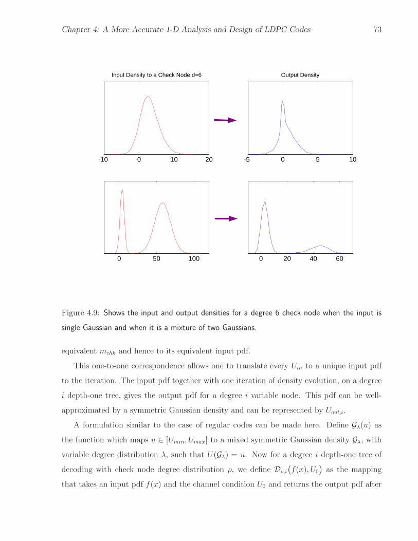
Chapter 4: A More Accurate 1-D Analysis and Design of LDPC Codes 73
-10 0 10 20
Input Density to a Check Node d=6
-5 0 5 10
Output Density
0 20 40 600 50 100
Figure 4.9: Shows the input and output densities for a degree 6 check node when the input is
single Gaussian and when it is a mixture of two Gaussians.
equivalent mchk and hence to its equivalent input pdf.
This one-to-one correspondence allows one to translate every Uin to a unique input pdf
to the iteration. The input pdf together with one iteration of density evolution, on a degree
i depth-one tree, gives the output pdf for a degree i variable node. This pdf can be well-
approximated by a symmetric Gaussian density and can be represented by Uout,i.
A formulation similar to the case of regular codes can be made here. Define Gλ(u) as
the function which maps u ∈ [Umin, Umax] to a mixed symmetric Gaussian density Gλ, with
variable degree distribution λ, such that U(Gλ) = u. Now for a degree i depth-one tree of
decoding with check node degree distribution ρ, we define Dρ,i
(
f(x), U0
)
as the mapping
that takes an input pdf f(x) and the channel condition U0 and returns the output pdf after

Chapter 4: A More Accurate 1-D Analysis and Design of LDPC Codes 74
one iteration of density evolution on the depth-one tree of decoding. We can formulate our
analysis as
Uout,i = U(
Dρ,i
(
Gλ(Uin), U0
)
)
. (4.12)
Repeating the same thing for all variable degrees present in the code, we can find Uout,i
at the output of all variable node degrees. Now, our task is to compute Uout for the mixture
of all variable nodes. This task depends on the choice of U . For some choices of U such as
error probability, this is always simplified to a linear combination of Uout,i weighted by the
variable degree distribution. This is because, using Bayes’ rule, pout can be computed as
pout =∑
i≥2
Pr(degree = i) · Pr(error|degree = i) =∑
i≥2
λi · pout,i, (4.13)
where pout,i is the already-computed message error rate at the output of degree i variable
node. By computing pout, one point of the EXIT chart of the irregular code is computed.
A similar formulation can be used for the mean of the messages [24]. It has been shown
in [47] that when the messages have a symmetric pdf, mutual-information combines linearly
to form the overall mutual-information.
In this chapter, for analysis of the irregular case, we are most interested in representing
the results using pin-pout axes. This simplifies the analysis of the irregular case to the above-
mentioned linear combination and is more insightful than other parameters. Notice that
in the phase of approximation, any other measure can be used. In the remainder of this
chapter, by an EXIT chart, we mean a pin vs. pout EXIT chart unless otherwise stated.
According to (4.13), the EXIT chart for an irregular code is a linear combination of EXIT
charts for different variable degrees. As a result, we have a set of one-dimensional elementary
curves whose linear combination explains the convergence behaviour of the irregular code.
Fig. 4.10 shows an example of these elementary curves.
A comparison between the predicted convergence behaviour and the actual result, once
using the semi-Gaussian and once using the all-Gaussian method, is depicted in Fig. 4.11. As
expected, the all-Gaussian method shows significantly larger error in early iterations. The
semi-Gaussian method, however, is in close agreement with the actual results.

Chapter 4: A More Accurate 1-D Analysis and Design of LDPC Codes 75
0 0.05 0.1 0.15 0.2 0.250
0.05
0.1
0.15
0.2
0.25
Convergence Behavior for Different Variable Degrees SNR=-1.91dB, dc=6
Pin
Pou
t
d2
d3
d6
d8
d20 d30
d15
Figure 4.10: EXIT charts for different variable degrees on AWGN channel at −1.91dB when
dc = 6.
4.4 Design of Irregular LDPC Codes
Design of irregular LDPC codes which can outperform regular codes was first considered
in [17]. Different methods for designing irregular LDPC codes have been introduced and used
[13,24,28]. In this work EXIT charts are designed (shaped) to guarantee good performance
of the code. EXIT charts are even used in the design of good Turbo codes. For example, [46]
presents a rate 1/2 turbo code which approaches the Shannon limit to within 0.1dB.
In our one-dimensional framework, the design problem is simplified to a linear program.
Fixing the check degree distribution, we refer to the EXIT chart of a code whose variable
nodes are all of degree i by fi(x) and we call it an “elementary” EXIT chart. This name
has been chosen for contrast with the EXIT chart for an irregular code which is a mixture

Chapter 4: A More Accurate 1-D Analysis and Design of LDPC Codes 76
0 0.05 0.1 0.15 0.2 0.250
0.05
0.1
0.15
0.2
0.25
Pin
Pou
t
Convergence Behavior of an Irregular Rate 0.248 Code at SNR=−2.2dB
Actual resultsAll Gaussian AssumptionHalf Gaussian Assumption
λ2 =0.20
λ3 =0.24
λ6 =0.16
λ20
=0.10λ
30=0.30
ρ
6=1.00
Figure 4.11: Actual convergence behaviour of an irregular code compared with the predicted
trajectory using the semi-Gaussian and the all-Gaussian methods.
of elementary EXIT charts. According to (4.13), the EXIT chart of an irregular code with
variable degree distribution λ = {λ2, λ3, . . .}, can be written as
f(x) =∑
i≥2
λifi(x).
This fact simplifies the problem of designing an irregular code to the problem of shaping
an EXIT chart out of a group of elementary EXIT charts. We wish to maximize the rate of the
code while having the EXIT chart of the irregular code satisfy the condition that f(x) < x for
all x ∈ (0, p0], where p0 is the initial message error rate at the decoder. Satisfying f(x) < x
for all x guarantees convergence to zero message error rate for an infinite blocklength code.
The design rate of the code is R = 1 −∑
ρj/j∑
λi/iand hence, for a fixed check degree distri-

Chapter 4: A More Accurate 1-D Analysis and Design of LDPC Codes 77
bution, the design problem can be formulated as the following linear program:
maximize∑
i≥2 λi/i
subject to λi ≥ 0,∑
i≥2 λi = 1, and
∀pin ∈ (0, p0](∑
i≥2 λifi(pin) < pin
)
.
In the above formulation, we have assumed that the elementary EXIT charts are given.
In practice, to find these curves we need to know the degree distribution of the code. We
need the degree distribution to associate every input pin to its equivalent input pdf, which
is in general assumed to be a Gaussian mixture. In other words, prior to the design, the
degree distribution is not known and as a result, we cannot find the elementary EXIT charts
to solve the linear program above.
To solve this problem, we suggest a recursive solution. At first we assume that the input
message to the iteration, Fig. 4.5, has a single symmetric Gaussian density instead of a
Gaussian mixture. Using this assumption, we can map every message error rate at the input
of the iteration to a unique input pdf and so find fi(x) curves for different i. It is interesting
that even with this assumption the error in approximating the threshold of convergence,
based on our observations, is less than 0.3dB and the codes which are designed have a
convergence threshold of at most 0.4dB worse than those designed by density evolution. One
reason for this is that when the input of a check node is mixture of symmetric Gaussians,
due to the computation at the check node, its output is dominated by the Gaussian in the
mixture having smallest mean.
After finding the appropriate degree distribution based on single Gaussian assumption we
use this degree distribution to find the correct elementary EXIT charts based on a Gaussian
mixture assumption. Now we use the corrected curves to design an irregular code. In this
level of design, the designed degree distribution is close to the used degree distribution in
finding the elementary EXIT charts. Therefore, analyzing this code with its actual degree
distribution shows minor error. One can continue these recursions for higher accuracy.
However, in our examples after one iteration of design the designed threshold and the exact
threshold differed less than 0.01 dB. So we propose the following design algorithm.
Algorithm:

Chapter 4: A More Accurate 1-D Analysis and Design of LDPC Codes 78
1. Map every pin to the associated symmetric Gaussian density (a single Gaussian).
2. Find the EXIT charts for different variable degrees.
3. Find a linear combination with an open EXIT chart that maximizes the rate
and meets all the required design criteria.
4. Use this degree sequence for mapping pin to the appropriate input densities
(a Gaussian mixture).
5. Find the EXIT charts for different variable degrees.
6. Find a linear combination with an open EXIT chart that maximizes the rate
and meets all the required design criteria.
4.5 Examples and Numerical Results
As an example, we consider designing an irregular code with the maximum possible rate
for a channel at SNR= 1σ2
n= −1.91 dB. We also want the code to have regular check degree
and use no variable node degree greater than 30. These restrictions constrain the decoding
complexity to a practically acceptable level. As noticed in previous work [13, 24], the check
degrees of the best codes designed using density evolution are either regular or concentrated
around one degree. Usually we choose the average check node degree and we build this
average using only two check degrees. Chung, et al., provide guidelines for choosing the
average check degree [24].
Fig. 4.13, shows the elementary EXIT charts when check nodes have degree 8. It can be
seen that a code design with maximum variable node 30 is not possible in this case because
the EXIT chart for variable nodes of degree 30 is barely open. As an experimental rule, the
check degree should be chosen in a way that the elementary EXIT chart associated with a
variable degree equal to ⌊max(dv)4
⌋ is about to close.
It can be seen from Fig. 4.14 that a check degree of 7 is not a good choice while from
Fig. 4.10 it can be seen that a check node degree of six is a good choice. Now, using the
curves on Fig. 4.10, which are computed based on a single Gaussian assumption at the input
of check nodes, we design a code using linear programming. The designed variable degree
sequence is presented in Table 4.3. Having the degree distribution of this code we find the

Chapter 4: A More Accurate 1-D Analysis and Design of LDPC Codes 79
00.
050.
1
Pin
0.15
0.2
0.25
0
0.050.1
Pou
t0.150.2
0.25
Sin
gle
Gau
ssia
n A
ssum
ptio
n
Mix
ture
Gau
ssia
n A
ssum
ptio
n
Act
ual C
urve
s
Figure 4.12: Illustrates the improved accuracy of elementary exit charts when a Gaussian mixture
assumption is made on the messages.

Chapter 4: A More Accurate 1-D Analysis and Design of LDPC Codes 80
0 0.05 0.1 0.15 0.2 0.250
0.05
0.1
0.15
0.2
0.25
Convergence Behavior for Different Variable Degrees SNR=-1.91dB, dc=8
Pin
Pou
t
d2
d3
d6
d8
d15
d30
d20
Figure 4.13: Shows elementary EXIT charts for different variable degrees on AWGN channel at
−1.91dB when dc = 8.
exact elementary EXIT charts for each variable degree. Fig. 4.12 compares the exact curves
with the approximated curves under single Gaussian assumption. Using exact curves we
repeat the design and achieve a new degree sequence. Since the curves used in the design are
based on another degree sequence, we have compared the actual curves for this final design
with the curves which are, in fact, used for this design in Fig. 4.12. This figure shows that
the approximation at this level of design is highly accurate.
According to Table 4.3 the designed code has a gap of about 0.14 dB from the Shannon
limit. The best codes designed using density evolution with maximum variable degree of
30 have a gap of about 0.09 dB from the Shannon limit when the rate of the code is 0.5
[13]. Unfortunately, to the best of our knowledge, there is no published rate one-third code
designed by density evolution. So, a more fair comparison is not possible here. Nevertheless,
this comparison shows that our one-dimensional approach does about as well as methods
based on density evolution under any practical measure.
We have used our design method to design a number of irregular codes with a variety
of rates. The results are presented in Table 4.4. In the design of the presented codes, we

Chapter 4: A More Accurate 1-D Analysis and Design of LDPC Codes 81
0 0.05 0.1 0.15 0.2 0.250
0.05
0.1
0.15
0.2
0.25
Convergence Behavior for Different Variable Degrees SNR=-1.91dB, dc=7
Pin
Pou
t
d2
d3
d6
d8
d20
d30
d15
Figure 4.14: Shows elementary EXIT charts for different variable degrees on AWGN channel at
−1.91dB when dc = 7.
have added some additional constraints, which makes the designed codes more practical for
implementation. We have avoided any variable or check nodes with degrees higher than
40. We have limited the number of used degrees to 10, favouring results which use fewer
check/variable degrees. For check nodes there has been no intention to make it regular, but
as long as it has been possible to design a code with regular check side with a performance
loss less than 0.01 dB, we have favoured a regular structure. Interestingly all the codes have
a regular structure at the check side. In the design of each code, we have maximized the
code rate for a given channel SNR.
Table 4.4 suggests that for code rates less than 0.25, the method shows noticeable in-
accuracy. However, for a wide range of rates it is quite successful. For rates greater than
0.85, getting close to capacity requires high-degree check nodes. To show that our method
can actually handle high rate codes, we designed a rate 0.9497 code, which uses check nodes
of degree 120 but no variable node of degree greater than 40. The variable degree sequence
for this code is λ = {λ2 = 0.1029, λ3 = 0.1823, λ6 = 0.1697, λ7 = 0.0008, λ9 = 0.1094, λ15 =
0.0240, λ35 = 0.2576, λ40 = 0.1533}. The threshold of this code is at σn = 0.4462, which

Chapter 4: A More Accurate 1-D Analysis and Design of LDPC Codes 82
Table 4.3: Irregular codes designed by Semi-Gaussian method for a Gaussian channel with
SNR=−1.91 dB
Degree Sequence Based on Single Gaussian Based on Gaussian Mixture
λ2 0.2754 0.2669
λ3 0.1647 0.2123
λ6 0.1331 0.1094
λ8 0.1026 0.1441
λ9 0.0829 0.0263
λ15 0.0175 0.0284
λ20 0.0348 0.0277
λ30 0.1890 0.1849
ρ6 1.0000 1.0000
Code Rate 0.3227 0.3407
Gap to the 0.486 0.139
Shannon Limit (dB)
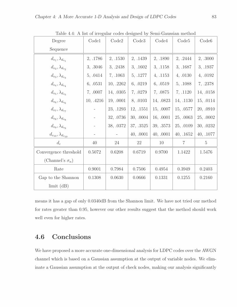
Chapter 4: A More Accurate 1-D Analysis and Design of LDPC Codes 83
Table 4.4: A list of irregular codes designed by Semi-Gaussian method
Degree Code1 Code2 Code3 Code4 Code5 Code6
Sequence
dv1 , λdv12, .1786 2, .1530 2, .1439 2, .1890 2, .2444 2, .3000
dv2 , λdv23, .3046 3, .2438 3, .1602 3, .1158 3, .1687 3, .1937
dv3 , λdv35, .0414 7, .1063 5, .1277 4, .1153 4, .0130 4, .0192
dv4 , λdv46, .0531 10, .2262 6, .0219 6, .0519 5, .1088 7, .2378
dv5 , λdv57, .0007 14, .0305 7, .0279 7, .0875 7, .1120 14, .0158
dv6 , λdv610, .4216 19, .0001 8, .0103 14, .0823 14, .1130 15, .0114
dv7 , λdv7- 23, .1293 12, .1551 15, .0007 15, .0577 20, .0910
dv8 , λdv8- 32, .0736 30, .0004 16, .0001 25, .0063 25, .0002
dv9 , λdv9- 38, .0372 37, .3525 39, .3573 25, .0109 30, .0232
dv10 , λdv10- - 40, .0001 40, .0001 40, .1652 40, .1077
dc 40 24 22 10 7 5
Convergence threshold 0.5072 0.6208 0.6719 0.9700 1.1422 1.5476
(Channel’s σn)
Rate 0.9001 0.7984 0.7506 0.4954 0.3949 0.2403
Gap to the Shannon 0.1308 0.0630 0.0666 0.1331 0.1255 0.2160
limit (dB)
means it has a gap of only 0.0340dB from the Shannon limit. We have not tried our method
for rates greater than 0.95, however our other results suggest that the method should work
well even for higher rates.
4.6 Conclusions
We have proposed a more accurate one-dimensional analysis for LDPC codes over the AWGN
channel which is based on a Gaussian assumption at the output of variable nodes. We elim-
inate a Gaussian assumption at the output of check nodes, making our analysis significantly

Chapter 4: A More Accurate 1-D Analysis and Design of LDPC Codes 84
more accurate than previous approaches. Compared to the previous work on one-dimensional
analysis of LDPC codes, our method not only offers better precision, but also can be used
over a wider range of rates, channel SNRs and maximum variable degrees.
We compared different measures for including the Gaussian assumption and showed that
the mutual information measure allows us to analyze the convergence behaviour of LDPC
codes very accurately and predict the convergence threshold within a few thousandths of a
dB from the actual threshold.
We used EXIT charts based on message error rate to design irregular LDPC codes.
Our one-dimensional analysis gives a deep insight to each level of design and the designed
code performs as well as codes designed using methods based on density evolution. Since our
analysis is not based on simplicity of check nodes, we believe it can be used for designing other
codes defined on graphs, such as irregular turbo codes [18], repeat-accumulate codes [19],
concatenated tree codes [16], or when more complicated check codes are employed in an
LDPC structure.

Chapter 5
EXIT-Chart Properties of the
Highest-Rate LDPC Code with
Desired Convergence Behaviour
In the previous two chapters, we saw that EXIT chart analysis can be very effective in
analysis and design of LDPC codes. In Chapter 3 we studied a case for which EXIT chart
analysis was exact. There exist other cases for which a one-dimensional analysis is exact, for
example belief propagation in the BEC. In general, whenever the density of messages can be
expressed by a single parameter, a one-dimensional analysis—tracking the evolution of that
parameter—is an exact analysis. We refer to such decoding schemes as “one-dimensional”
decoding schemes.
Even when the decoding scheme is not one-dimensional, a one-dimensional analysis can
be used to approximate the behaviour of such decoders, as we did in Chapter 4. In both cases
we showed that the irregular code design problem can be formulated as a linear program.
However, we have not so far studied or discussed the shape or the properties of the EXIT
chart of the designed code.
The main goal of this chapter is to study the properties of the EXIT chart of the designed
irregular codes. We start with reviewing the existing results, which are limited to the case of
the BEC and then will present our results. Although the results of this chapter are strictly
85

Chapter 5: EXIT-Chart Properties of the Highest-Rate LDPC Code 86
valid only for one-dimensional decoding schemes, they can still be used within the framework
of any one-dimensional approximation of other decoding schemes.
5.1 Background and Problem Definition
The properties of EXIT charts for the BEC are studied in [50]. The main result of [50] is that
the area under the EXIT chart scales with the rate of the code. Prior to [50], it was known
that for the BEC a capacity-achieving LDPC code has a truly flat EXIT chart, i.e., its first
derivative approaches one and its higher derivatives approach zero everywhere [20]. That is
to say the EXIT chart of a capacity achieving code on the BEC is almost closed everywhere,
and hence an infinite number of iterations is required to achieve any target error rate. It
was also known that capacity achieving codes have infinitely long degree distributions [21];
indeed, it is known that a truly flat curve cannot always be achieved using finite degree
distributions.
Although these results are only for the case of the BEC, it seems that a similar concept
is still valid for other channels. For example, Fig. 5.1 compares the EXIT charts of two
irregular codes under sum-product decoding on the same AWGN channel. One can see that
the higher rate code has a “flatter” EXIT chart.
In this work we relate the EXIT chart of an irregular LDPC code to its rate without
considering a specific decoding rule. Inevitably, our results cannot be as strong as the
existing results for the BEC, but their general nature is their advantage.
5.2 Problem Formulation
As we showed in Chapter 3 and Chapter 4, an EXIT chart based on the message error rate
has the nice property of reducing the irregular code design to a linear program, given that
the check degree distribution is fixed.
Here, we assume a 1-to-1 relation between message error rate and the parameter defining
the message distribution of the one-dimensional decoder. This will allow an EXIT chart
representation based on message error rate. Thus, in the remainder of this chapter an EXIT

Chapter 5: EXIT-Chart Properties of the Highest-Rate LDPC Code 87
0 0.06 0.12 0.180
0.06
0.12
0.18
pin
p out
Code 1, λ4=0.6, λ
40=0.4, R=0.375
Code 2, λ4=0.3, λ
14=0.5, λ
40=0.2,R=0.136
AWGN Channel, SNR=0.26dB, dc=10
Figure 5.1: Comparison of EXIT charts for two irregular codes.
chart is defined as a curve that, for a fixed channel condition, represents pout as a function
of pin, i.e., pout = f(pin).
We refer to the EXIT chart of a code with a fixed variable degree i by fi(x) and we call
it an elementary EXIT chart (as opposed to the EXIT chart of an irregular code which is
a combination of elementary EXIT charts). The EXIT chart of an irregular code with the
variable degree distribution λ = {λi, i ∈ I}, I = {2, . . . , I}, can be written as
f(x) =∑
i∈I
λifi(x).
Here, we have considered a finite set I because, an infinitely long degree distribution
cannot be implemented in a finite blocklength code. In practice, one need to consider a
finite degree sequence, and studying the properties of the EXIT chart of such irregular code

Chapter 5: EXIT-Chart Properties of the Highest-Rate LDPC Code 88
would be most interesting.
5.2.1 Desired convergence behaviour
Unlike previous work on irregular code design that only considers convergence to zero error
rate, we treat here the general case of code design with a desired convergence behaviour.
This allows for the tradeoff of code rate for convergence performance. To see this, suppose
the EXIT chart f(x) of a code is very close to x, for example ax < f(x) < x, and a → 1−, as
would be the case for capacity-approaching sequences for the BEC [20]. It is clear that after
n iterations a lower bound on the message error rate would be p0an, and so a large number of
iterations, on the order of 1| log(a)|
, is required to achieve a small message error rate. Hence, in
general one might be interested in trading code rate for decoding complexity. Thus, we will
be interested in the maximum rate code while guaranteeing a specific convergence behaviour
described by h(x).
The design problem is, then, equivalent to shaping an EXIT chart out of a group of
elementary EXIT charts that maximize the rate of the code while having the EXIT chart
of the irregular code below h(x), i.e., satisfying f(x) ≤ h(x) for all x. This guarantees a
performance at least as good as the required one. If convergence to zero error rate is required,
then h(x) must satisfy h(x) < x for all x in the convergence region (0, p0], where p0 is the
intrinsic message error rate.
With a minor modification, the design linear program can be rewritten as:
maximize∑
i∈I λi/i
subject to λi ≥ 0,∑
i∈I λi = 1, and
∀pin ∈ [0, p0](∑
i∈I λifi(pin) ≤ h(pin))
.
Letting x = pin/p0, the region of interest for x is [0, 1].
In the rest of this chapter we make the following assumptions: fi(x), h(x) and fi(x)/h(x)
are continuous functions over [0,1] and ∃x ∈ [0, 1] such that f2(x) > h(x). The latter
assumption is made to avoid a trivial problem. Otherwise, the highest rate code uses only
degree two variable nodes.
Chapter 5: EXIT-Chart Properties of the Highest-Rate LDPC Code 89
5.2.2 Monotonic Decoders
Definition 5.1 A decoder is called monotonic if for any j > i, fj(x) ≤ fi(x) for x ∈ [0, 1].
This definition is justified because any reasonable message-passing scheme should consider
all the information it receives in each variable node and make use of it. Suppose that at a
degree i node, the input-output relation is given by pout = fi(pin). At a degree j > i node we
can have the same input-output relation by throwing away j − i input messages and using a
similar message-passing rule. Hence, for a reasonable decoder, the input-output relation for
a variable node of degree j should be at least as good as that of any lower variable degree
node. Thus, fj(pin) should be less than or equal to fi(pin) for all pin, where j > i. Therefore,
in this work, we are only interested in those decoders which are monotonic.
5.3 Results
Theorem 5.1 Among all codes satisfying a convergence behaviour h(x), i.e.,
∀pin ∈ [0, p0] ,
(
∑
i∈I
λifi(pin) ≤ h(pin),
)
there exists a maximal rate code.
Proof: It is well known that any continuous function over a closed bounded set achieves
a maximum. The set of “admissible” variable degree distributions
Λ : λi ≥ 0,∑
i∈I λi = 1
∀x ∈ [0, 1]∑
i∈I λifi(x) ≤ h(x)
is a closed and bounded set, and∑
λi/i (or equivalently the rate) is continuous. Hence, the
highest rate is achievable.
Definition 5.2 Let {fi(x) : i ∈ I} be the set of elementary EXIT charts and h(x) be the
desired convergence behaviour curve. A variable degree distribution Λ = {λi : i ∈ I} is called
critical with respect to h(x) if there exists x ∈ [0, 1] such that
∑
i∈I
λifi(x)
h(x)= 1.

Chapter 5: EXIT-Chart Properties of the Highest-Rate LDPC Code 90
Notice that∑
i∈I λifi(x)h(x)
= 1 is a stronger statement than∑
i∈I λifi(x) = h(x). For example,
when∑
i∈I λifi(x) = h(x) = 0, the former statement requires that the first derivatives of
h(x) and∑
i∈I λifi(x) at x (if they exist) should be equal to each other.
Theorem 5.2 Let {fi(x) : i ∈ I} be the set of elementary EXIT charts and h(x) be the
desired convergence-behaviour curve. Suppose Λ = {λi : i ∈ I} is an admissible variable
degree distribution achieving the highest rate. Then Λ is critical with respect to h(x).
Proof: Since Λ is an admissible variable degree distribution,
∀x ∈ [0, 1] ,∑
i∈I
λifi(x) ≤ h(x).
As a result,∑
i∈I
λifi(x)
h(x)≤ 1.
Suppose, to the contrary, that Λ is not critical. Then
∀x ∈ [0, 1] ,∑
i∈I
λifi(x)
h(x)< 1.
By the continuity of∑
i∈I λifi(x)h(x)
over the interval [0, 1], there exists ǫ > 0 such that
∑
i∈I
λifi(x)
h(x)≤ 1 − ǫ.
Now, we are going to construct another admissible variable degree distribution which has a
higher rate than Λ, causing a contradiction.
Let
κ = maxx∈[0,1]
f2(x)
h(x).
As Λ is admissible, there exists n > 2 such that λn > 0. Define a variable degree distribution
Ψ = {ψi : i ∈ I} as follows:
ψ2 = λ2 + min( ǫκ, λn)
ψn = λn − min( ǫκ, λn)
ψi = λi otherwise.
Clearly∑
i∈I ψi = 1 and ψi ≥ 0. It can also be verified that
∑
i∈I
ψifi(x)
h(x)≤
∑
i∈I
λifi(x)
h(x)+ min(
ǫ
κ, λn)
f2(x)
h(x)≤ 1.
Chapter 5: EXIT-Chart Properties of the Highest-Rate LDPC Code 91
Therefore, Ψ is admissible. In addition, it has a rate strictly greater than rate of Λ because
∑
i∈I
ψi
i=
∑
i∈I
λi
i+ min(
ǫ
κ, λn)(
1
2− 1
n).
Hence, a contradiction occurs.
Now, consider a scenario where there are two variable degree distributions Λ and Ψ such
that the rate of Λ is greater than the rate of Ψ and the EXIT chart of Λ is always below the
chart of Ψ. This means that Λ is better than Ψ in all aspects. A good code should avoid
using degree distributions which offer a lower rate and at the same time has an EXIT chart
closer to the 45-degree line. To be more specific we make the following definition.
Definition 5.3 Let J be a subset of I. If for every set of real numbers {δj : j ∈ J }, which
satisfies∑
j∈J δj = 0 and∑
j∈J δjfj(x) ≤ 0 for all x ∈ [0, 1], we have∑
j∈Jδj
j≤ 0, we say
J is consistent with respect to the set of elementary EXIT charts F = {fi(x) : i ∈ I}. If Fis known from the context, we simply say J is consistent.
If, J is inconsistent then there exists a set of real numbers {δj : j ∈ J } such that∑
j∈J δj = 0,∑
j∈J δjfj(x) ≤ 0 for all x ∈ [0, 1] and∑
j∈Jδj
j> 0.
For any admissible variable degree distribution Λ = {λi : i ∈ I}, its support J is defined
by {j ∈ I : λj > 0}.
Theorem 5.3 Let Λ = {λi : i ∈ I} be the highest rate admissible degree distribution. Then
its support is consistent.
Proof: Let J be the support of Λ. If J is not consistent, then by definition, there exists
{δj : j ∈ J } such that∑
j∈J δj = 0,∑
j∈J δjfj(x) ≤ 0 for all x ∈ [0, 1] and∑
j∈Jδj
j> 0.
Let ǫ = maxj∈J |δj|, τ = minj∈J |λj|. Let Ψ = {ψi : i ∈ I} be a variable degree distribution
where ψj equals to λj + τǫδj for j ∈ J and equals to zero otherwise. It is obvious that
∑
i∈I ψi =∑
i∈ λi = 1. For any j ∈ J ,
ψj = λj +τ
ǫδj ≥ λj −
τ
ǫ|δj| ≥ 0.
On the other hand, by definition,

Chapter 5: EXIT-Chart Properties of the Highest-Rate LDPC Code 92
∑
j∈J
ψjfj(x) =∑
j∈J
λjfj(x) +τ
ǫ
∑
j∈J
δjfj(x) ≤ h(x).
Hence, Ψ is admissible. This causes a contradiction, because the rate associated with Ψ is
greater than the rate of Λ since
∑
j∈J
ψj
j=
∑
j∈J
λj
j+
τ
ǫ
∑
j
δj
j>
∑
j∈J
λj
j.
Let Ψ = {ψi : i ∈ I} and Λ = {λi : i ∈ I} be two variable degree distributions. We
define a partial order relation “ ≻” as follows: Λ ≻ Ψ if and only if the union of the support
of Λ and Ψ is consistent, and for all x ∈ [0, 1],∑
i∈I λifi(x) ≥ ∑
i∈I ψifi(x). When Λ ≻ Ψ,
we say Λ dominates Ψ.
Corollary 1 Suppose J is consistent. Let Λ and Ψ be two admissible variable degree dis-
tributions with support being subsets of J . If Λ ≻ Ψ, then the rate of Λ is greater than or
equal to the rate of Ψ.
Proof: Let Γ = {γi = ψi − λi : i ∈ I}. Then∑
j∈J γj = 0, and∑
j∈J γjfj(x) ≤ 0.
Thus, by the consistency of J ,∑
j∈Jγj
j≤ 0, or equivalently
∑
j∈Jλj
j≥ ∑
jψj
j.
5.4 Discussion and Examples
Let us compare our results with the existing results for the BEC channel. For the BEC
we know that the maximum rate code has a flat EXIT chart [20]. We showed that in the
general case, the EXIT chart of the maximum rate code has to meet the desired convergence
behaviour curve at least at one point. For the BEC we know that the area under the EXIT
chart scales with the rate of the code [50]. We showed that for two irregular codes C1 and
C2, whose supports are subsets of a consistent set J , if the EXIT chart of C1 is always above
that of C2 then C1 has a higher rate. That is to say if the EXIT chart of a code C is equal
to h(x) it is the highest rate code which guarantees this convergence behaviour among all
codes whose support is a subset of J .

Chapter 5: EXIT-Chart Properties of the Highest-Rate LDPC Code 93
Choosing h(x) = x results in the highest code rate, but has impractical decoding com-
plexity. Hence, here we considered general h(x). Relaxing h(x) reduces the complexity at
the expense of rate loss. Given a target error rate and a maximum affordable complexity,
one interesting open question is to find the best h(x) which results in the highest code rate.
We finish this chapter with two examples which show some of our results in the case
of code design for Gallager’s Algorithm B. We discussed code design for Algorithm B in
Chapter 3. Here, we only present the designed codes.
Example 1: On a BSC with a crossover probability of 0.04 and under Algorithm B, we
want to design an LDPC code whose check nodes are all degree 10 and its maximum variable
node degree is no more than 12. We assume h1(x) = x as the desired convergence behaviour.
The result of this design is {λ2 = 0.0052, λ3 = 0.0877, λ4 = 0.8543, λ11 = 0.0528}, with
a code rate of 0.6004. The EXIT chart of this code is plotted in Fig. 5.2 (Code 1) and
is compared with its desired convergence behaviour. As it can be seen, the EXIT chart is
critical with respect to its desired convergence behaviour at three points, which are indicated
with pointers on the figure.
Example 2: Consider the previous example, but this time assume h2(x) = 0.8x as the
desired convergence behaviour.
The result of code design in this case is {λ2 = 0.0180, λ3 = 0.1269, λ4 = 0.5087, λ11 =
0.3464}, with a code rate of 0.5237. The EXIT chart of this code is also plotted in Fig. 5.2
(Code 2) and is compared with its desired convergence behaviour. Again, it can be seen
that the EXIT chart of this code is critical with respect to its desired convergence behaviour
at three points. Another observation from Fig. 5.2 is that, the EXIT chart of Code 1 (the
higher rate code) dominates that of Code 2.

Chapter 5: EXIT-Chart Properties of the Highest-Rate LDPC Code 94
00.
010.
020.
030.
040
0.01
0.02
0.03
0.04
p in
pout
h 1(x)
= x
Cod
e 1,
Rat
e 0.
6004
h 2(x)=
0.8
x
Cod
e 2,
Rat
e 0.
5237
Figure 5.2: Comparison of EXIT charts for two irregular codes, which are designed with different
desired convergence behaviour curves.

Chapter 6
Near-Capacity Coding in
Multi-Carrier Modulation Systems
In previous chapters, we showed the application of LDPC codes to some channel types. In
all cases, however, we assumed a binary LDPC code. In Chapter 4 we saw that irregular
LDPC codes can approach the capacity of binary modulation on a Gaussian channel very
closely. In the high SNR regime, however, using binary modulation is not spectrally efficient.
To approach the capacity of the channel, higher-order modulation schemes should be used.
Coding for higher-order modulation schemes can be done either by use of non-binary codes
or by multi-level coding, which allows the use of binary codes. Each of these solutions have
their own advantages and disadvantages. However, a multi-level coding approach seems to
be more appropriate for LDPC coding. This is mainly because it allows for the use of long
blocklength codes, it can approach capacity very closely, the decoding complexity is much
less and design of binary irregular LDPC codes is easier or at least more studied.
In a discrete multi-tone (DMT) system in a frequency-selective channel, the superiority
of a multi-level coding approach is even more obvious. This is because different tones may
need different modulation schemes, hence different signaling alphabets. A multi-level coding
system, however, can use binary codes regardless of the modulation formats used in the
different tones.
In this chapter we apply irregular LDPC codes to the design of multi-level coded quadra-
95

Chapter 6: Near-Capacity Coding in Multi-Carrier Modulation Systems 96
ture amplitude modulation (QAM) schemes for application in DMT systems in frequency-
selective channels. We use a combined Gray/Ungerboeck scheme to label each QAM con-
stellation. The Gray-labelled bits are protected using an irregular LDPC code with iterative
soft-decision decoding, while other bits are protected using a high-rate Reed-Solomon code
with hard-decision decoding (or are left uncoded). The rate of the LDPC code is selected
by analyzing the capacity of the channel seen by the Gray-labelled bits, and is made adap-
tive by selective concatenation with an inner repetition code. Using a practical bit-loading
algorithm, we apply this coding scheme to an ensemble of frequency-selective channels with
Gaussian noise. Over a large number of channel realizations, this coding scheme provides
an average effective coding gain of more than 7.5 dB at a bit error rate of 10−7 and a block
length of about 105 bits. This represents a gap of approximately 2.3 dB from the Shannon
limit of the additive white Gaussian noise channel, which could be closed to within 0.8 to
1.2 dB using constellation shaping.
This chapter is the result of a joint work with Tooraj Esmailian which will be published
as a regular paper in IEEE Trans. on Commun. [51]. Some of the results of this chapter
are reported in [52]. There have been a number of modification as well as new contributions
in this work, since [52]. While the main focus of [52] is on power-line channels, our focus
is on the coding part of the proposed system. We have revised some of the parameters of
the coding system to improve our presentation. In addition we have added an analysis of
complexity and delay of the system and made some of the discussions clearer. The purpose
of repeating some of the old results is to make this chapter more accessible, as the new
contributions are in continuation of the previously reported results.
This chapter is organized as follows. In Section 6.1, we briefly review some aspects of
multilevel coding. In Section 6.2, our channel model is briefly discussed. In Section 6.3, we
explain the structure of our proposed system. In Section 6.4, we present the specifications
of our system for an ensemble of frequency-selective channels encountered in power-line
channels [53]. Section 6.5 shows some simulation results and finally some conclusion remarks
are presented in Section 6.6.

Chapter 6: Near-Capacity Coding in Multi-Carrier Modulation Systems 97
6.1 Background
DMT systems have special requirements which makes the design of coding systems for them
a challenge [54–56]. In standard asymmetric digital subscriber lines [57], the error control
coding is based on a trellis-coded-modulation scheme in concatenation with a Reed-Solomon
code, which provides approximately 5 dB of coding gain at a symbol error rate of 10−7.
The SNR gap between performance of the uncoded quadrature amplitude modulation
(QAM) and the Shannon limit on the AWGN channel is approximately 9 dB at a symbol
error rate of 10−6. At this symbol error rate, the coding gain of the Leech lattice in dimension
24 is less than 4 dB [58] and a 512-state trellis code can provide a coding gain of almost 5.5 dB.
Approaching a coding gain close to 6 dB with trellis codes seems to be very difficult [58]. All
the coding gains that we refer to are only due to coding. Using proper shaping techniques, a
shaping gain of up to 1.53 dB can be added independent of the coding gain. However, even
with a 512-state trellis code and achieving the ultimate shaping gain, there is a gap of 2 dB
from the Shannon limit.
The goal of this chapter is to provide near-capacity coding techniques for high-SNR regime
and more generally for DMT systems. At low SNR, the problem of near-capacity coding
has been studied extensively and a group of codes, including turbo codes and LDPC codes,
has been found that can approach the capacity of many channels with practical complexity.
For high-SNR channels, however, non-binary modulation is required. The main problem of
using multilevel symbols in turbo codes and LDPC codes is that large alphabet sizes create
prohibitively large decoding complexity. To overcome this problem one can use multilevel
coding, which allows one to apply binary codes to multilevel modulation schemes. However,
in DMT systems, dealing with sub-channels with various SNRs is different and use of different
constellation sizes is a challenge.
6.1.1 Our approach
There has been some other work in this area. In [59], regular high rate LDPC codes are used
in digital subscriber line (DSL) transmission systems and a coding gain of 6.2 dB at a bit
error rate of 10−7 is reported. Compared to the maximum possible coding gain (8.3 dB for the

Chapter 6: Near-Capacity Coding in Multi-Carrier Modulation Systems 98
AWGN channel), this amounts to a gap of more than 2 dB from the Shannon limit. The goal
of [59] is to provide a coding system for DSL transmission systems with practical complexity
and suitable structure for hardware implementation, so highly efficient irregular codes, which
are more difficult to implement, were not considered. The idea of using LDPC codes together
with coded modulation has also been proposed in [60] for use in ADSL. The system described
in [60] illustrates substantial coding gains relative to trellis-coded modulation, but does not
appear to use optimized LDPC codes such as those suggested in this work. In [55], turbo
codes are used with coded modulation and a coding gain of 6 dB at symbol error rate of
10−6 (equivalent to approximately 6.8 dB at a symbol error rate of 10−7 or 1.5 dB gap from
the Shannon limit for the AWGN channel) is reported for ADSL systems.
In this chapter, using a combination of irregular LDPC codes and multilevel coding, we
propose a coding scheme which provides an average coding gain of more than 7.5 dB at a
message error rate of 10−7 (equivalent to a gap of approximately 0.8 dB from the Shannon
limit for the AWGN channel). The decoding complexity in our system is comparable with a
512-state trellis code.
The main difference between our approach and other work on use of turbo codes/LDPC
codes for DMT systems is that our main goal is to maximize the coding gain for a practical
decoding complexity. For this purpose, motivated by [61, 62], after labelling symbols with
binary sequences, we model an effective channel—which will be referred to as a bit-channel—
for each bit level of the label. Then, for different constellation sizes, we compute the capacity
of the bit-channels that each label bit sees. This allows us to choose an efficient error-
correcting code for each level bit whose code rate accounts for the capacity of the associated
bit-channel.
Another difference is that we do not use a single code for all the label bits. We use
the powerful LDPC coding only for those label bits that need this high-complexity coding
scheme. As a result, we propose a quasi-multilevel coding system. We use a single LDPC
code for the least significant bits of the label, but higher level bits are coded with less complex
codes. This is equivalent to bit-interleaved coded modulation for least significant bits of the
label and multilevel coding for higher level bits. It should be mentioned that bit-interleaved
coded modulation together with a Gray-labelling can perform very close to multilevel coding

Chapter 6: Near-Capacity Coding in Multi-Carrier Modulation Systems 99
with set partitioning labelling [63].
Another benefit of this strategy is that we avoid high rate LDPC codes. High rate
irregular LDPC codes need a very high check degree in order to be able to perform near
capacity. This is because in high rate codes, the number of check nodes (compared to the
number of variable nodes) is small. High degree check nodes introduce a large number of
short cycles in the factor graph of the code, which adversely affects the performance of finite
length codes.
Moreover, instead of choosing from a set of codes with different rates at each channel
condition, we employ a fixed rate LDPC code that is selectively concatenated with a repeti-
tion code to provide a flexible overall coding rate for the system. This is necessary, since for
some realizations of the channel the capacity of the bit-channels assigned to the LDPC code
can be less than the rate of the LDPC code. The repetition code is used only for bit-channels
whose capacity is very low.
In terms of hardware implementation, compared to the approach in [59], which uses highly
structured LDPC codes in a multilevel coding system, our system is more complex because
we use constellations of size 2l where l can be an even or odd integer. In addition, our LDPC
code is irregular. Although our decoding complexity is similar, the encoding complexity in
our system is higher because we have not used codes with algebraic properties.
All the above differences have allowed us to approach capacity much more closely. More-
over, our system works for a very wide range of channel conditions because it has a flexible
code rate.
6.1.2 Multilevel coding
The main idea of multilevel coding is based on the concept of set partitioning [64]. Assume
that the points of a constellation A = {a0, a1, . . . , aM−1} of M = 2l points is labelled with a
binary address b = (b0, b1, . . . , bl−1). The idea of multilevel coding is to protect the address
bits bi’s by using binary codes. Usually, every address bit bi is protected with an individual
code Ci [61].
Notice that there is a one-to-one mapping between an address vector b and a constellation
Chapter 6: Near-Capacity Coding in Multi-Carrier Modulation Systems 100
point A, hence, if we denote the transmitted signal with random variable A and the received
signal with another random variable Y , then the mutual information I(Y ; A) is equal to the
mutual information between Y and b. Therefore
I(Y ; A) = I(Y ; b0, b1, . . . , bl−1)
= I(Y ; b0) + I(Y ; b1|b0) + · · · + I(Y ; bl−1|b0, b1, . . . , bl−2). (6.1)
Hence, transmission of the address vector can be viewed as separate transmission of individ-
ual binary address bits bi’s. Thus, each address bit sees an effective channel (bit-channel)
whose capacity can be different from the other bit-channels due to the labelling scheme.
At the decoder, according to (6.1), the mutual information I(Y ; b0) is used in order to
decode b0. Then the conditional mutual information I(Y ; b1|b0) is used to decode b1. That
is to say, the capacity of the second bit-channel has to be defined conditioned on the first
address bit. In general for the ith bit-channel the capacity is defined conditioned on b0 to
bi−1. If set partitioning labelling, e.g., an Ungerboeck-labelling, is used for bit labels, then
conditioned on b0, b1 sees a higher capacity bit-channel than b0. Hence, a higher rate code
can be used for b1 than for b0. At the next stage, conditioned on both b0 and b1, b2 sees
an even higher capacity bit-channel, and so on. Therefore, label bits must be protected by
different rate codes. It is known that if each code achieves the capacity of its bit-channel,
the total capacity of the channel is achieved [61]. Fig. 6.1 shows the net capacity of 4-QAM
and 8-QAM signalling together with the capacity of each bit-channel as a function of SNR
assuming that an Ungerboeck-labelling is used. We refer the reader to [65,66] for a complete
study of these systems and a more detailed structure of the encoder and decoder for such
systems.
Fig. 6.2 shows the general structure of a multilevel encoder and Fig. 6.3 shows the general
structure of a multistage decoder. At the transmitter side the binary inputs are partitioned
into l sub-blocks. Each of these sub-blocks are passed to a different binary encoder. The l
output bits of these l encoders are used to address a point from a 2l points constellation.
At the receiver, the first decoder decodes the first address bits. The second decoder uses
these bit as well as the received symbols to decode second-level bits. Continuing in the same
fashion, all levels will be decoded.

Chapter 6: Near-Capacity Coding in Multi-Carrier Modulation Systems 101
5 10 15 20 250
1
24 QAM
Cap
acity
(bi
ts/s
ymbo
l) Bit-Channel 0 Bit-Channel 1 Signal-Channel
5 10 15 20 250
1
2
3
SNR (dB)
Cap
acity
(bi
ts/s
ymbo
l)
8QAM
Bit-Channel 0 Bit-Channel 1 Bit-Channel 2 Signal-Channel
Figure 6.1: Net capacity and capacities associated with bit-channels (bit-channel 0: I(Y ; b0),
bit-channel 1: I(Y ; b1|b0), bit-channel 2: I(Y ; b2|b0, b1)) for 4-QAM/8-QAM signalling when an
Ungerboeck-labelling is used.
Notice that, after decoding the first bit, the sub-constellation chosen by this bit has a
larger minimum Euclidean distance. Hence, a higher rate code compared to the first level
code, can be used for the second level bits. For a similar reason, an even higher code rate
can be used for higher level bits.
6.2 Channel Model
Although the approach of this work in terms of providing a near-capacity coding system for
DMT systems is quite general, we consider in-building power-line channels as an example
and our focus in the design will be this class of channels.
A detailed study of characteristics of in-building power-line channels has been conducted
in [53], and a stochastic ensemble of test channels described. The parameters of the test
channels are based on limitations placed on wiring configurations by the National Electric

Chapter 6: Near-Capacity Coding in Multi-Carrier Modulation Systems 102
Symbol
−1
0b
l −1
1bEncoder
Encoder. . .
0
1
Dat
aP
artit
ioni
ng
Map
ping
Encoderb
Input
Bits
Output
l
Figure 6.2: General structure of a multilevel encoder.
Code, by the size and type of building in which the power-lines are located, by the expected
load impedances, and by experimental measurement of background and impulsive noise.
We use the channel model provided in [53] to generate our sample test channels. We also
use the distribution of channel SNR provided in [53] for our system design. To show the
success of our design, we present results for different size buildings and different realizations
of the channel. Fig. 6.4 shows the magnitude of the frequency response of three representative
test channels. For more details about the parameters of these channels, see [53].
This application to power-line channels is intended to be representative only, and we
expect the results of this work to apply to broad classes of frequency-selective Gaussian
channels.
6.3 System Structure
Equation (6.1) is one of many different ways that one can partition the total capacity to
the capacity of single bits. As discussed before, this suggests using an Ungerboeck labelling
together with separate codes for each level of the label bits. Constellation labelling and

Chapter 6: Near-Capacity Coding in Multi-Carrier Modulation Systems 103
Input
−1
0b
1b
l −1b
1Decoder
Decoder0
Decoder
. . . . . .. . .
Symbols
l
Figure 6.3: General structure of a multilevel decoder.
decoding stages strongly depends on the way that one partitions the total capacity.
Since we wish to perform near the capacity of the channel we consider using LDPC codes
for different levels of the label bits. However, we avoid using a single code for each address
bit because decoding higher level bits is not possible without finishing the decoding for lower
level bits. As a result, to avoid a long decoding delay, the length of the employed LDPC
codes should be relatively small, which hinders the performance of the code. This is because
the performance of LDPC codes depends on their block length. The larger the block length,
the closer the performance of the code to the capacity. For instance, with a block length of
105 there is a gap of about 0.2 dB to the predicted performance, and with a block length of
106 this gap is reduced to 0.05 dB [13].
An alternative solution for our system is bit-interleaved coded modulation, i.e., to use
a single code for all label bits without partitioning the total capacity to sum of bit-channel
capacities. Bit-interleaved coded modulation together with a Gray-labelling can approach
the channel capacity very closely [63], but unlike multilevel coding cannot achieve it. The
capacity of the Gray-coded channel for various constellation sizes and number of coded bits
is analyzed in [67].
Assigning all label bits to one LDPC code has some disadvantages. For instance, it
requires a high rate LDPC code which can perform close to capacity only with high degree
check nodes. High degree check nodes introduce short cycles in the factor graph of the

Chapter 6: Near-Capacity Coding in Multi-Carrier Modulation Systems 104
5 10 15 20 25 30−45
−40
−35
−30
−25
−20
−15
−10
Frequency (MHz)
Cha
nnel
freq
uenc
y re
spon
se a
mpl
itude
(dB
)
Small building Meduim buildingLarge building
Figure 6.4: The magnitude of the frequency response of three test channels (same as Fig. 6.11
of [52]).
code and hinders the performance. Another problem with bit-interleaved coded modulation
is that in terms of decoding complexity it may not be an efficient solution. Notice that
the capacity of higher bit-channels under set partitioning labelling can be very close to
one (typically more than 0.95 bits/symbol). Hence, some bit-channels can effectively be
protected by low-complexity codes such as Reed-Solomon codes and some bit-channels can
be left uncoded.
Considering these facts, we propose using a single code for only two least significant bits.
This way, we can double the length of the code (compared to the case that single LDPC codes
are used for each level bits) for the same delay and hence have a better performance. Notice
that the LDPC decoding complexity scales linearly with the length of the code. Hence, the
complexity per bit of information is independent of the code length. Encoding and decoding
these two bits together is equivalent to bit-interleaved coded modulation for these two bits.
Hence, a Gray-labelling must be used in order to approach the capacity very closely [63]. In

Chapter 6: Near-Capacity Coding in Multi-Carrier Modulation Systems 105
b0b
1b
2b
3
0000
1111
0110
1000 0010 1010
0100 1100 1110
0011 1011 0001 1001
0111 0101 1101
Figure 6.5: Labelling of a 16-QAM constellation in our system.
other words these two address bits will have equal minimum Euclidean distance and almost
equal error probability, which allows the use of a single LDPC code for them.
We use Ungerboeck-labelling for higher level bits to further increase the capacity for even
higher address bits. This provides us with some bit-channels whose raw error rate is very
low and can be coded with low complexity high rate codes and some bit-channels whose raw
error rate is better than the target error rate of the system and hence do not need any coding.
This will further reduce the overall complexity of the system. In this work, only b2 and b3
need protection and higher address bits are not coded. Fig. 6.5 shows the labelling used for
a 16-QAM constellation in our system. Notice that for b2 and b3 an Ungerboeck-labelling is
used.
It should be mentioned that, in practice, a relatively large number of sub-channels use
4-QAM signalling. Thus, including address bits other than b0 and b1 in the LDPC code
does not contribute much in the length of the LDPC code (since they are absent in many
sub-channels) yet increases the complexity of the system.
Based on the above discussion, we rewrite (6.1) as:
I(Y ; b0, b1, . . . , bl−1) = I(Y ; b0, b1) + I(Y ; b2|b0, b1) + · · · + I(Y ; bl−1|b0, b1, . . . , bl−2). (6.2)

Chapter 6: Near-Capacity Coding in Multi-Carrier Modulation Systems 106
Map
ping
b
l −1b
4b
3b
0b 1b
Input
Bits Dat
aP
artit
ioni
ng
Buffer
Buffer
LDPC EncoderRate 0.6
RS Encoder
BufferRS Encoder
. . .
(255 209)
(255 241)
Output
Symbols
2
Figure 6.6: The block diagram of the encoder of the proposed system.
For b0 and b1 the average bit-channel capacity can be computed as
Cb0b1 = log2(N/4)− 1
N
1∑
b1=0
1∑
b0=0
N4−1
∑
k=0
E
log2
N4−1
∑
i=0
exp
[
−|akb1b0
+ w − aib1b0
| − |w|22σ2
]
, (6.3)
where N is the number of points in the constellation, akb1b0
is the kth point on a sub-
constellation with fixed b1 and b0, and w represents samples of a complex Gaussian noise
with variance 2σ2.
Since the rate of the irregular LDPC code that we use is fixed and very close to the bit-
channel capacity, but the characteristics of the channel vary with time and frequency, we use
an inner rate 1/2 repetition code to take care of cases where the capacity of the bit-channels
assigned to the LDPC code is less than the rate of the LDPC code. The repetition code is
used only for bit-channels whose capacity is very low. In other words, our code (LDPC code
in concatenation with the repetition code) has an adaptive rate to guarantee convergence
over all channel realizations. Another advantage of the repetition code is that it allows the
use of low capacity bit-channels. This in turn allows us to switch to higher constellation
sizes at lower SNRs compared to previous work. As a result the system can perform even
closer to the capacity.
Figures 6.6 and 6.7 show the block diagram of the proposed system at the transmitter
and the receiver. At the transmitter, the constellation mapper uses two bits from the output
of LDPC encoder as the lowest address bits, and the outputs of encoder-2 to encoder-(l− 2)
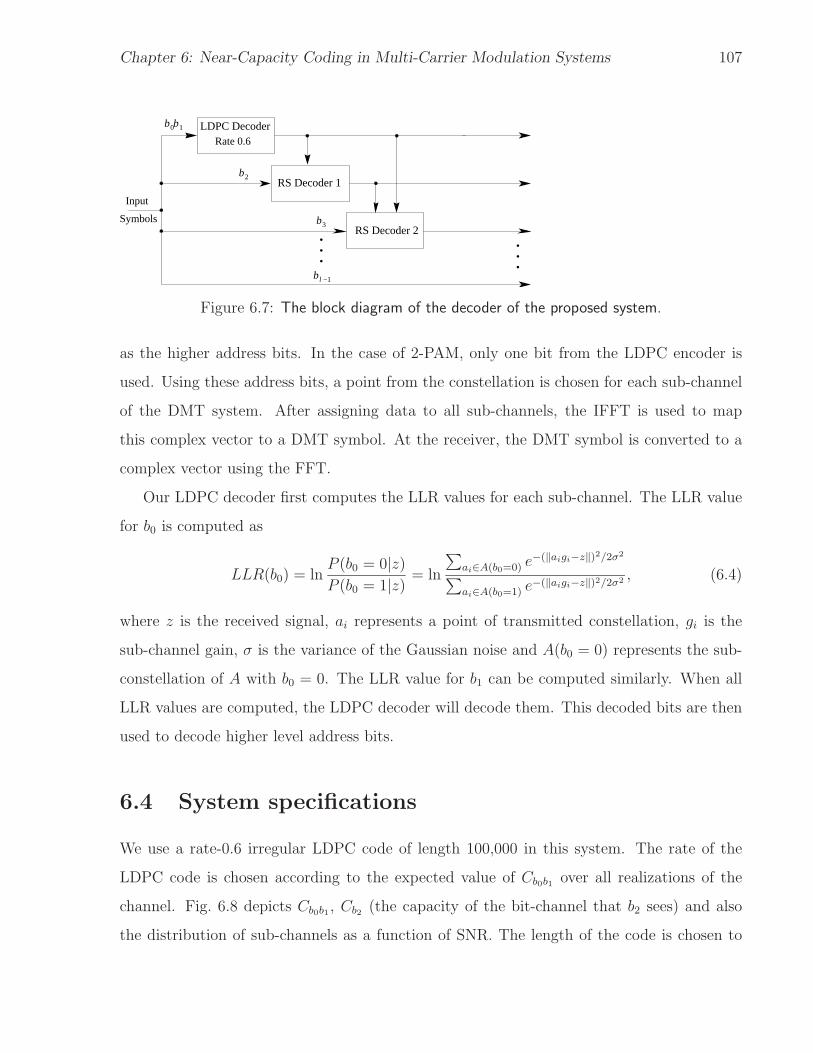
Chapter 6: Near-Capacity Coding in Multi-Carrier Modulation Systems 107
Input
b0b
2b
3b
l −1b
LDPC DecoderRate 0.6
RS Decoder 1
RS Decoder 2
. . .
. . .
Symbols
1
Figure 6.7: The block diagram of the decoder of the proposed system.
as the higher address bits. In the case of 2-PAM, only one bit from the LDPC encoder is
used. Using these address bits, a point from the constellation is chosen for each sub-channel
of the DMT system. After assigning data to all sub-channels, the IFFT is used to map
this complex vector to a DMT symbol. At the receiver, the DMT symbol is converted to a
complex vector using the FFT.
Our LDPC decoder first computes the LLR values for each sub-channel. The LLR value
for b0 is computed as
LLR(b0) = lnP (b0 = 0|z)
P (b0 = 1|z)= ln
∑
ai∈A(b0=0) e−(‖aigi−z‖)2/2σ2
∑
ai∈A(b0=1) e−(‖aigi−z‖)2/2σ2 , (6.4)
where z is the received signal, ai represents a point of transmitted constellation, gi is the
sub-channel gain, σ is the variance of the Gaussian noise and A(b0 = 0) represents the sub-
constellation of A with b0 = 0. The LLR value for b1 can be computed similarly. When all
LLR values are computed, the LDPC decoder will decode them. This decoded bits are then
used to decode higher level address bits.
6.4 System specifications
We use a rate-0.6 irregular LDPC code of length 100,000 in this system. The rate of the
LDPC code is chosen according to the expected value of Cb0b1 over all realizations of the
channel. Fig. 6.8 depicts Cb0b1 , Cb2 (the capacity of the bit-channel that b2 sees) and also
the distribution of sub-channels as a function of SNR. The length of the code is chosen to

Chapter 6: Near-Capacity Coding in Multi-Carrier Modulation Systems 108
have a tolerable delay for data applications. The system delay is mainly due to:
• buffer-fills in the LDPC encoder/decoder, which can be computed as
tbf =(LDPC code length) × (LDPC code rate)
(system bit rate) × (portion of bits assigned to the LDPC code)
• decoding delay: td =LDPC code lengthdecoder throughput
.
Compared to tbf and td, encoding delay, propagation delay and delay due to higher level
codes are negligible. Hence, the total delay can be approximated as 2tbf + td.
With a typical throughput of 100Mbps for the LDPC decoder, a minimum bit rate of 1
Mbps and assuming that 2/3 of bits are being passed to the LDPC code the overall delay is
approximately 181 ms. Hence the actual delay is not more than 190 ms. About 95% of this
delay is due to buffer-fills in the LDPC encoder/decoder. For higher bit rates, say 10 Mbps,
this delay is much shorter (approximately 19 ms) and the overall delay does not exceed
30 ms, which is acceptable even for voice applications. Here we assume that the channel has
the same ratio of coded to uncoded bits and the higher bit rate is due to a higher channel
bandwidth. A longer delay is expected, if the higher bit rate is due to (or partially due to)
a lower ratio of coded to uncoded bits on the channel.
From Fig. 6.8, it can be seen that b2 sees a channel whose capacity is very close to one,
which means that a high rate code can be used. The expected value of this capacity is about
0.986 bits/symbol and for b3 it is more than 0.999 bits/symbol. The capacity for higher
levels is even greater.
Many different types of codes can be used for these high capacity channels. One simple
solution is to use Reed-Solomon codes. A (255,209) Reed-Solomon code, with a rate more
than 0.819, can guarantee a frame error rate less than 10−7 for b2 and a (255, 241) Reed-
Solomon code, with a rate more than 0.945 can guarantee the same frame error rate for b3.
Hence the gap from capacity in these bit-channels is small. Also notice that, due to their
low SNR, many sub-channels do not have b2 and b3, so some rate loss in these bit-channels
does not dramatically impact the overall performance of the system.

Chapter 6: Near-Capacity Coding in Multi-Carrier Modulation Systems 109
6.4.1 Bit-loading algorithm
The bit-loading algorithm, i.e., the algorithm that chooses the constellation size at a given
SNR, affects the capacity of bit-channels. The bit-loading algorithm chooses the constellation
size in order to approach the total capacity as closely as possible. The zigzag form of bit-
channel capacities in Fig. 6.8 is due to the bit-loading algorithm, which switches to larger
constellations as the SNR increases. At each switch, the capacity of all address bits drops,
however the net capacity increases. This can be understood from Fig. 6.1. The capacity
of “bit-channel 0” and “bit-channel 1” in the case of 4-QAM is always greater than that
of 8-QAM. However, in the case of 8-QAM there is an extra bit-channel with a very high
capacity which makes the net capacity of 8-QAM greater than the net capacity of 4-QAM.
As a result, the bit-loading algorithm on the one hand wishes to switch to higher constel-
lation sizes to approach capacity more closely and on the other hand wishes to avoid higher
constellation sizes as they may lead to bit-channels with a very poor capacity. Higher con-
stellation sizes may also increase complexity. Hence, the bit-loading algorithm must trade
off between complexity and performance. Pseudocode for the bit-loading algorithm that we
have used is as follows.
Bit-Loading Algorithm:
1. Input: SNR, Threshold
2. set Constellation = MaximumConstellationSize
3. while { C(Constellation,SNR) - C(Constellation/2,SNR) ≤ Threshold}set Constellation = Constellation/2
4. Output: Constellation
Here the function C(Constellation,SNR) returns the capacity of a QAM constellation
of the given size at the given channel SNR. In our setting, the maximum constellation size
is 256-QAM, the threshold is 0.25 bits/symbol and we allow all constellation sizes of the
form 2l down to 2-PAM. As a result, our bit-loading algorithm assigns, at each SNR, the
minimum number of bits to each sub-channel in a way so that the constellation capacity is

Chapter 6: Near-Capacity Coding in Multi-Carrier Modulation Systems 110
less than 0.25 bit away from the capacity of the constellation one level higher. In this way
we make sure that we are quite close to the channel capacity with the minimum complexity
in terms of constellation size.
Fig. 6.8 also shows that, for different SNRs, the Cb0b1 varies approximately between 0.5
and 0.9 bits/symbol. Its average value over all realizations of the channel is about 0.68
bit/symbol. Hence we used a rate 0.6 LDPC code.
For any realization of the channel, one can think of each sub-channel as a random sample
from the sub-channel distribution of Fig. 6.8. The relatively large number of sub-channels
makes the average value of Cb0b1 for one channel realization close to the expected value on all
realizations. However, with a small probability, some realizations of channel can result in an
average Cb0b1 less than 0.6 bits/symbol. This is possible since each sub-channel, independent
of the other sub-channels, can have a capacity less than 0.6 bits/symbol.We use an inner
rate 1/2 repetition code for some sub-channels with very low capacity to make sure that the
same fixed-rate LDPC code can handle all channel realizations.
For a given realization of the channel, we first check the average of Cb0b1 . If it is less
than 0.66, we decide to employ the repetition inner code because the LDPC code may
not converge on its own. In every sub-channel, if Cb0b1 is less than a threshold value c0
(typically 0.5 bits/symbol), we repeat those bits. From the LDPC code point of view, this is
equivalent to sending a bit over a cleaner channel with a capacity almost doubled. Making
the simplifying assumption that the capacity in those sub-channels is actually doubled, we
compute the average Cb0b1 over all sub-channels again, and if it exceeds 0.7 we reduce the
threshold value c0; if it is less than 0.66 we increase the threshold value c0; otherwise we
proceed. This repetition algorithm makes the average capacity over all sub-channels to be
between 0.66 bits/symbol and 0.7 bits/symbol. In this way we maintain a reasonably small
gap from capacity for rate 0.6 LDPC code.
The degree distribution of the LDPC code that we have used in these system is Λ =
{λ2 = 0.229, λ3 = 0.234, λ6 = 0.217, λ15 = 0.320} and P = {ρ10 = 1} (the check side of the
code is regular with check nodes of degree 10). This degree distribution is derived under a
Gaussian assumption on the messages and the design method studied in Chapter 4.
We note that we cannot make the length of the LDPC code an integer multiple of the

Chapter 6: Near-Capacity Coding in Multi-Carrier Modulation Systems 111
length of the DMT symbols. This is because as the channel changes with time, the length
of the DMT symbols vary. To overcome this problem we simply put as many DMT symbols
as possible in the LDPC structure and fill the remaining portion of the LDPC code with
zeros. This has no significant effect of the system performance, because the typical size of
a DMT symbol (a few hundred bits), compared to the length of the code (100,000 bits), is
very small. One may use the fact that the code is zero-padded in order to perform a more
efficient decoding, but the improvement is minor.
6.4.2 System Complexity
Since the encoding/decoding complexity of the rather long LDPC code dominates the overall
complexity of the system, it will be our focus on this section.
The encoding complexity, when the code has some structure, is relatively small in com-
parison with the decoding complexity as the decoder needs a large number of iterations
(about 100 in our case). For example if the degree two variable nodes are chained to form
a structure similar to RA codes [19], the number of operations for encoding will be approx-
imately equal to the number of edges (400,000 in our case), while the decoder needs more
than this many operations per iterations. So the main focus of this complexity analysis will
be on the decoding complexity.
We saw in Chapter 2 that the update rules of the sum-product algorithm at a check node
c and a neighbouring variable node v are as follows:
mc→v = 2tanh−1(∏
h∈n(c)−{v}
tanh(mh→c
2)), (6.5)
mv→c = m0 +∑
y∈n(v)−{c}
my→v. (6.6)
From these equations, it can be shown that at a variable node of degree dv, 2dv operations
are enough to compute all the output messages. Notice that, one can add all dv + 1 input
messages in dv operations and then for every outgoing message one subtraction is required.
So another dv operations should be done. As a result the number of operations at the variable
side of the code is 2∑
v dv or equivalently 2E, where E is the number of edges in the graph.

Chapter 6: Near-Capacity Coding in Multi-Carrier Modulation Systems 112
Similarly, at a check node of degree dc, a total of 2(dc − 1) operations is needed. Hence,
at the check side of the code the number of operations is 2(E − C), where C is the number
of check nodes. Notice that (6.5) can be written as
tanh(mc→v
2) =
∏
h∈n(c)−{v}
tanh(mh→c
2), (6.7)
hence, having a lookup table or a circuit to map a message m to tanh(m/2) and back, the
situation is similar to a variable node. As a result, a total of 4E−2C operations per iteration
are required at the decoder. Considering a maximum of 100 iterations, the number of edges
(400,000) and the number of check nodes (40,000), the overall complexity of decoding is
152 Mega operations for 60,000 information bits, or 2534 operations per bit. Considering
complexities involved with other parts of the system we estimate an overall complexity of
fewer than 2700 operations per bit.
In our proposed system we have 4 coded bits whose overall rate is about 3/4. The
complexity of our system is comparable with the complexity of Viterbi decoding on a 512-
state trellis with an underlying rate 3/4 code. Such a trellis has 512 states and 8 branches
leaving each state. At each stage of the trellis the decoding involves one addition per branch
and 7 comparison per state of the trellis. That is 7680 operations per 3 information bits or
2560 operations per bit.
It has to be mentioned that the hardware complexity of the LDPC decoder is higher
than that of the Viterbi decoder as the LDPC decoder needs more memory. However, such
comparisons are highly implementation-dependant.
6.5 Simulation Results
We have used our proposed system on six samples of power-line channels results of our simula-
tions are reported in Table 6.1. In our simulation, we have assumed that the synchronization
and channel knowledge at the transmitter and receiver sides are perfect.
In Table 6.1, Cb0b1 is the average of (6.3) over all sub-channels and Rc is the overall code
rate used for b0b1. Notice that when the repetition code is not required, the overall code rate

Chapter 6: Near-Capacity Coding in Multi-Carrier Modulation Systems 113
is 0.6 bits/symbol, but when the average channel capacity is smaller than 0.66 bits/symbol,
the repetition code is active and the overall rate of the code is less than 0.6 bits/symbol.
In Table 6.1, lb shows the gap from the capacity of binary modulation. That is to say, if
a rate Rc code be used in a binary input AWGN channel whose capacity is Cb0b1 , lb is the
gap from the Shannon limit. We also define excess redundancy (ER) as another measure of
performance. In each sub-channel, excess redundancy is the difference between the capacity
of that sub-channel (in bits/channel-use) and the information bits which are actually assigned
to it. The average excess redundancy on all sub-channels is denoted by ER which can be
computed as
ER =1
N
N∑
i=1
[log2(1 + SNRi) −ni
∑
j=1
Rbj,i] . (6.8)
Here, N is the number of sub-channels, SNRi is the SNR of the ith sub-channel, ni is
the number of bits transmitted in the ith sub-channel, and Rbj,iis the code rate used for
the jth bit of ith sub-channel. Since ER directly measures the gap from the capacity in
bits/channel-use, it is a good measure of performance for a coding scheme.
In many other work in the coded-modulation literature, coding gain is represented as
a measure of performance. In our case however, there is no standard way to compute the
coding gain, because sub-channels with different SNRs are used. However, considering a
DMT channel with N sub-channels whose capacities are given by C1 to CN , and comparing
it with a second DMT system whose sub-channels all have the same capacity C, we have
C = 1N
∑Ni=1 Ci for the two systems to have equal capacity. Now, assume SNRi for sub-
channel i on the first system and SNReff for all the sub-channels of the second DMT system.
Using C = log2(1 + SNR), we get:
1 + SNReff = N
√
√
√
√
N∏
i=1
(1 + SNRi).
When SNR values are large enough this can be simplified to
SNReff = N
√
√
√
√
N∏
i=1
SNRi. (6.9)
Or in other words, SNReff is the geometric mean of the SNRi’s. Now, comparing an uncoded
system with a system which uses coding, if we denote the effective SNR after coding with

Chapter 6: Near-Capacity Coding in Multi-Carrier Modulation Systems 114
Channel Cb0b1 Rc Decoding Iterations lb (dB) ER (bits) G (dB)
Small 0.69 0.60 90 0.58 0.41 7.51
Medium 0.71 0.60 70 0.68 0.43 7.15
Large 0.69 0.60 80 0.58 0.36 7.56
Medium 1 0.65 0.57 100 0.56 0.37 7.67
Medium 2 0.57 0.50 100 0.61 0.23 8.09
Medium 3 0.75 0.60 50 1.15 0.56 6.52
Table 6.1: Simulation results on six power-line channels.
SNRc,eff in dB and if each sub-channel has a coding gain of Gi in dB, then the required SNR
for ith sub-channel is SNRi − Gi so we have:
SNRc,eff = SNReff − 1
N
N∑
i=1
Gi
so our average coding gain in dB is G = 1N
∑Ni=1 Gi. This is in dB which in linear form would
be the geometric average of the sub-channels coding gain. To find the coding gain in each
sub-channel we first compute the gap from the Shannon limit as
Li =SNRi
2∑ni
j=1 Rbj,i − 1. (6.10)
Since the uncoded SNRnorm for QAM modulation at at a bit error rate of 10−7 is 9.8 dB, the
coding gain on this sub-channel at this bit error rate is Gi = 100.98/Li. Hence, the effective
coding gain is G = N
√
∏Ni=1 Gi . This effective coding gain is also reported in Table 6.1.
It worth mentioning that at high SNRs there is a gap of about 1.53 dB between mod-
ulation capacity and the capacity of the Gaussian channel [58]. This can be reduced using
shaping techniques [68–70]. The gap at lower SNRs is smaller. In a DMT system, which has
sub-channels with different SNRs, this gap is less than 1.53 dB on average.
The channel frequency response of the first three test channels of the table, which are
derived from buildings with different sizes, is shown in Fig. 6.4. The next three test channels,
which are from medium size buildings, are selected to show special cases. Two of them are
selected to have a Cb0b1 less than 0.66 so that the repetition code becomes active. As

Chapter 6: Near-Capacity Coding in Multi-Carrier Modulation Systems 115
mentioned before, this happens with a small probability. The last test channel is selected to
have a high Cb0b1 . Such a high Cb0b1 is also very rare.
6.6 Conclusion
In this chapter we have proposed a high performance error-correction system suitable for
DMT systems. In our system, we label QAM constellation points using a combined Gray/
Ungerboeck labelling scheme. Low-order bits are coded with an irregular LDPC code, which
is selectively concatenated with a repetition code to provide an adaptive rate. The rate of
the LDPC code is carefully chosen based on the capacity of the corresponding bit-channels.
Higher-order bits are coded with Reed-Solomon codes, or are left uncoded. We provide a
practical bit-loading algorithm, that maintains a balance between constellation complexity
and coding efficiency. The decoding complexity of the system is comparable to that of a
traditional trellis-coded modulation scheme with 512 states. Using our scheme, performance
is achieved equivalent to a gap of approximately 2.3 dB from the Shannon limit without con-
stellation shaping, on a class of channels encountered in power-line communication systems.
This gap could be closed to about 1 dB with appropriate shaping methods. Our approach
applies not only to power-line channels, but to general frequency-selective channels; hence
we believe a similar system can be considered for high SNR wireless channels or digital
subscriber-line channels.

Chapter 6: Near-Capacity Coding in Multi-Carrier Modulation Systems 116
0 5 10 15 20 25 300
0.2
0.4
0.6
0.8
1Average Capacity of b
0 and b
1
SNR (dB)
Cap
acity
(B
its/S
ymbo
l)
0 5 10 15 20 25 300.85
0.9
0.95
1Capacity of b
2
SNR (dB)
Cap
acity
(B
its/S
ymbo
l)
4QAM
8QAM
16QAM
32QAM
64QAM
128QAM
256QAM
Bit−Loading AlgorithmDecision
8QAM
16QAM
32QAM
64QAM
128QAM
256QAM
Bit−Loading AlgorithmDecision
−20 −15 −10 −5 0 5 10 15 20 25 300
0.02
0.04
0.06
0.08
0.1Probability Density Function of Sub−Channels SNRs
SNR (dB)
Figure 6.8: Shows Cb0b1 , bit-channel capacity for b2 and the PDF of sub-channels as a function
of SNR.

Chapter 7
Gear-Shift Decoding
In previous chapters, our focus was mainly on the design of good LDPC codes for a given
decoding scheme. In this chapter, we focus on the design of less complex decoders for a
given LDPC code, without sacrificing performance. We discussed the possibility of using soft
decoding rules in early iterations and hard decoding rules in later iterations of decoding in
Chapter 2. In this chapter we show that, by allowing the decoder to choose its decoding rule
among a group of decoding algorithms, we can speed up the decoding process significantly.
There are many different message-passing algorithms with varying performance and com-
plexity. High-complexity decoding algorithms such as sum-product can correct more errors
created by the channel noise, so they are very attractive when complexity and computation
time is not an issue. Low-complexity decoding algorithms, however, are more attractive
when we need fast decoders for delay-sensitive applications or high-throughput systems.
Low-complexity decoding rules have two main drawbacks. First, they have a worse
threshold of decoding compared to high-complexity algorithms so, to ensure convergence,
a lower code rate should be used. Second, due to their relatively poor performance, more
iterations of such algorithms are required to achieve a given target bit error rate. Hence, it
is not obvious if the overall computations are any less.
Now consider the following scenario: a long blocklength regular (4,8) LDPC code is
used to protect data transmitted over a Gaussian channel whose SNR is 2.50 dB. Four
different decoding algorithms—sum-product, min-sum, Algorithm E (erasure in the decoder)
117

Chapter 7: Gear-Shift Decoding 118
[12] and Algorithm B—are implemented in software. Based on these implementations, the
computation times of these algorithms are 5.2, 2.8, 0.9 and 0.39 µsecond per bit per iteration
(µs/b/iter), respectively.
A routine analysis shows that we need 9 iterations of sum-product decoding to achieve a
target message error rate of less than 10−7. That is to say, the decoding time is 46.8 µs/b.
Using min-sum decoding, density evolution analysis shows that 20 iterations are required,
hence the decoding time will be 56.0 µs/b. It can be easily verified that using Algorithm
E or Gallager’s Algorithm B, the decoding will fail. Notice that although min-sum is a
lower-complexity algorithm, its overall decoding time is longer.
Now assume that the decoder is allowed to vary its decoding strategy at each iteration.
Using density evolution, one can verify that performing 4 iterations of sum-product, followed
by 5 iterations of Algorithm E and followed by 4 iterations of Algorithm B the decoder will
achieve the same target error rate with a computation time of just 26.86µs/b. This is less
than 58% of the time required by a sum-product decoder and is more than twice as fast as
a min-sum decoder. It also makes use of Algorithms E and B, which are very fast decoding
algorithms, but which could not be used on their own for this channel condition.
We call the strategy of switching from one algorithm to another “gear-shift decoding” as
the decoder changes gears (its algorithm) in order to speed up the decoding process.
In this chapter, we consider an iterative message-passing decoder that can choose its de-
coding rule among a group of decoding algorithms at each iteration (for example: a software
decoder). Each available decoding algorithm may have a different computation time and
performance. Given a set of decoding algorithms and their computation time, we discuss
how to find the optimum combination in the sense of minimizing the decoding time. We also
prove that the optimum gear-shift decoder (the one with the minimum decoding-latency)
has a decoding threshold equal to or better than the best decoding threshold of the available
algorithms. We use extrinsic information transfer charts and dynamic programming to find
the optimum gear-shift decoder. We then show that, with some modifications, gear-shift
decoding can be used to design pipeline decoders with minimum hardware cost for a given
throughput.
This chapter is organized as follows. In Section 7.1 we define and solve the gear-shift

Chapter 7: Gear-Shift Decoding 119
decoding optimization problem for minimum decoding-latency. The minimum hardware
design problem, is defined and solved in Section 7.2. Section 7.3 presents some examples
and Section 7.4 concludes the chapter.
7.1 Gear-shift decoding
Gear-shift decoding, simply put, means allowing the decoder to change its decoding algorithm
during the process of decoding. Gear-shift decoding for LDPC codes, interestingly, dates back
to Gallager and his original work on LDPC codes [11]. For binary message-passing decoders,
Gallager noticed that, by allowing a decision threshold to be changed during the process of
decoding, the decoder’s performance and convergence threshold improves significantly. We
did a detailed study of this gear-shifting algorithm of Gallager, i.e., Algorithm B in Chapter
3 and, in fact, we showed that it is the optimum decoding rule when the messages are binary.
The importance of using different decoding algorithms in the case of binary message-
passing has inspired other work. In hybrid decoding [71], the variable nodes are partitioned,
with nodes in different partitions performing a different algorithm. This results in an average
behaviour which can be better than the convergence behaviour of every single algorithm.
In soft decoding, however, it is well known that sum-product decoding minimizes error
probability when the factor graph of the code is cycle free. Thus, gear-shift decoding can-
not help to improve the threshold of convergence beyond the threshold of the sum-product
decoding. However, as we discussed earlier, the complexity of decoding can be reduced by
gear-shift decoding.
In this section, assuming that an EXIT chart analysis is accurate enough, we show how
to find the optimum gear-shift decoder. We present our EXIT charts based on message
error probability, because this approach reflects typical design goals. For instance, one can
request a target message error rate rather than a target SNR or mutual information. Thus,
in the remainder of this chapter, we assume that the EXIT charts are tracking the extrinsic
message error rate. An mentioned in previous chapters, such an EXIT chart can be thought
as a function
pout = f(pin, p0), (7.1)

Chapter 7: Gear-Shift Decoding 120
where p0 is the intrinsic message error rate, pin is the extrinsic message error rate at the input
of the iteration and pout is the extrinsic message error rate at the output of the iteration.
7.1.1 Definitions and assumptions
Consider a set of N different decoding algorithms numbered from 1 to N whose EXIT charts
are given as fi(pin, p0), for 1 ≤ i ≤ N . The computation time for one iteration of algorithm
i is ti, which is assumed to be independent of pin and p0.
A gear-shift decoder is denoted with a sequence of integers S,
S = (a1, a2, . . . , al(S)), ai ∈ {1, 2, . . . , N},
which means algorithm number a1 is used in the first iteration, algorithm number a2 is used
in the second iteration, etc. The computation time for such a gear-shift decoder is
TS =
l(S)∑
i=1
tai,
and the output message error rate of such a decoder is
PS(p0) = fal(S)
(
fal−1(S)
(
. . . fa2(fa1(p0, p0), p0), . . .)
, p0
)
. (7.2)
Notice that initially the extrinsic message error rate is equal to p0.
For a given target message error rate pt, we say a gear-shift decoder S is admissible
if PS(p0) ≤ pt. The “optimum gear-shift decoder” corresponds to the sequence S∗ whose
computation time is less than all other admissible sequences.
We assume that EXIT charts are increasing functions of pin and p0. This is because,
a greater pin (p0), i.e., having more extrinsic (intrinsic) message errors at the input of an
iteration, usually results in more message errors at the output of the iteration, i.e., a greater
pout. We also assume that the output messages of each algorithm are compatible with the
input of each algorithm.
7.1.2 Equally-complex algorithms
If all the decoding rules have equal computation time, i.e., ti is a constant, it is clear that
the optimum gear-shift decoder at each iteration uses the algorithm whose output extrinsic

Chapter 7: Gear-Shift Decoding 121
message error rate is the smallest of all. Using EXIT charts, we are able to pictorially compare
the success of different algorithms in each iteration and find the best one. Algorithm B for
LDPC codes is a good example for this case.
We introduced Algorithm B in Chapter 2 and studied it in more detail in Chapter 3.
Here we just provide one example to serve the purpose of this chapter and show two things:
(1) the concept of gear-shift decoding in Algorithm B, (2) the convenience of using EXIT
charts in the design of gear-shift decoders.
Consider a (dv,dc) regular LDPC code and assume that the messages are binary valued.
At a check node, the outgoing message is the modulo-two sum of the incoming messages. At
a variable node, the outgoing message is the same as the channel message unless at least b
of the extrinsic messages disagree, where ⌈dv/2⌉ ≤ b ≤ dv − 1. For example, for a (4,8) code,
there are two decoding rules, corresponding to b = 2 and b = 3.
Recall that Gallager suggests to choose parameter b in iteration l as the smallest integer
that satisfies1 − p0
p0
<
[
1 + (1 − 2p(l−1))dc−1
1 − (1 − 2p(l−1))dc−1
]2b−dv+1
,
where p0 is the intrinsic error rate and p(l) is the extrinsic error rate at iteration l. We can
also plot the EXIT charts of the different decoding rules and decide where to change b. To
see the convenience of this approach, consider a (4,8) code. The EXIT charts of the two
algorithms discussed above (b = 2 and b = 3) for p0 = 0.03 are plotted in Fig. 7.1.
One can see that the EXIT chart for b = 2 is closed, but it has a better convergence
behaviour than b = 3 for small extrinsic message error rates. A routine analysis shows that,
with b = 3, we need 27 iterations to achieve a target message error rate of 10−7. Figure 7.1,
however, suggests switching to b = 2, after 4 iterations with b = 3. This way, another 5
iterations with b = 2 is required for achieving the same target error rate. As a result, the
decoding speed is improved by a factor of three. Another fact which can be easily verified
analytically is that the decoding threshold for b = 2 is at p0 = 0.0077 and for b = 3 is at
p0 = 0.0476, while for Algorithm B it is at p0 = 0.0515. When 0.0476 < p0 < 0.0515, none
of the two algorithms can converge, but the decoding becomes possible when the decoder is
allowed to choose between the two different rules.

Chapter 7: Gear-Shift Decoding 122
0 0.01 0.02 0.030
0.01
0.02
0.03
Gallager’s Algorithm B (4,8) Code, P0=0.03
Pin
Pou
t
b=2b=3
Figure 7.1: Compares the convergence behaviour of two different binary message passing algo-
rithm.
It can be easily proved that the greedy strategy of choosing the algorithm with the
best performance in each iteration (independent of other iterations) results in the fastest
convergence.
Theorem 7.1 Given a channel condition p0 and a set of equally complex algorithms, a
greedy algorithm achieves the target error rate in the least time.
Proof: Given a gear-shift decoder S = {a1, a2, . . . , al}, 1 ≤ ai ≤ N , using (7.2), one
can compute PS(p0), i.e., the message error rate after l iterations.
Now assume that S∗ = {a∗1, a
∗2, . . . , a
∗l } represents the sequence associated with the greedy
algorithm of the same length l. If S∗ is not the best sequence for l iterations, we call the best
sequence S = {a1, a2, . . . , al}. Now change S as follows. At the first place where S differs

Chapter 7: Gear-Shift Decoding 123
with S∗, say in iteration i, switch ai with a∗i , leaving the rest of S unchanged and call the
updated sequence S∗. Since S∗ is based on a greedy decision,
fa∗
i(p
(i−1)out , p0) < fai
(p(i−1)out , p0),
where p(i−1)out shows the output message error probability after the first i−1 iterations. Notice
that these first i−1 iterations are the same in both S∗ and S so p(i−1)out is the input error rate
to both S and S∗ at iteration i.
Since all EXIT charts are assumed to be increasing functions of pin, it is evident that
after l iterations S∗ offers a better pout than S, which contradicts the assumption that S is
the best decoding sequence. Therefore, S∗ has the minimum message error rate among all
sequences of length l. Since l was chosen arbitrarily, S∗ achieves a better error rate for any
l iterations and hence meets the target error rate in the least number of iterations.
7.1.3 Algorithms with varying complexity
When the computation times of different algorithms are not equal, it is not clear which
combination of algorithms will result in the fastest decoding. Choosing the algorithm with
the best performance may cost a lot of computation while for the same amount of compu-
tation another algorithm could produce better results. In this section we show that, finding
the sequence of algorithms with the minimum computational complexity can be cast as a
dynamic program. We first define the problem.
We use the general setup of Section 7.1.1. At a fixed p0, for each EXIT function fi(pin, p0),
we define a quantized version fi(pin) whose domain and range is the set P = {p0, p1, . . . , pn}.Here, p0 is the intrinsic message error rate, p0 > p1 > · · · > pn and pn is equal to pt the
target message error rate. For pin = pm, 0 ≤ m ≤ n we define
fi(pin) ,
p0 if fi(pin, p0) ≥ p0
pk otherwise,
where k, k ∈ {0, . . . , n} is the largest integer for which fi(pin, p0) ≤ pk. This way fi is
a pessimistic approximation of fi, hence an admissible gear-shift decoder based on f ’s is
guaranteed to achieve pt.

Chapter 7: Gear-Shift Decoding 124
p0
p1
p2
p3
p4
p5
Algorithm 1
Algorithm 3Algorithm 2
Figure 7.2: A simple trellis of decoding performance with P of size 6 and 3 algorithms. Notice
that some of the states have fewer than 3 outgoing edges. This happens when some algorithms
have a closed EXIT chart at this message error rate.
We form a trellis whose states are the elements of P and whose branches are formed by f .
From each state we have N branches associated with the N available decoding algorithms.
Each branch, associated with algorithm i, connects state pm in time T to state pk in time
T + 1 if and only if fi(pm) = pk. The weight of such a branch is ti. We refer to this trellis
as the “trellis of decoding performance”.
Any path in this trellis which starts at p0 and ends at pn = pt defines an admissible
gear-shift decoder whose computation time is the sum of the weights of branches on that
path. The optimum gear-shift decoder is associated with the path of minimum weight, which
can be found by dynamic programming.
Notice that the number of branches in this trellis is proportional to N and n, so increasing
n, in order to reduce the quantization error, linearly increases the number of trellis branches.
As a result having even thousands of states can be effectively handled.
Another point is that we are interested only in the minimum weight path from p0 to pn,
hence we can remove all branches that connect a state pm at time T to a state pk at time
T + 1 when pk ≥ pm. This further simplifies the dynamic program. An example trellis of
decoding performance is shown in Fig. 7.2.

Chapter 7: Gear-Shift Decoding 125
7.1.4 Convergence threshold of the gear-shift decoder
For equally complex algorithms, it is clear that the convergence threshold of the gear-shift
decoder is equal to or better than the best of the available decoders. Note that the decoder
chooses the most open EXIT chart at each iteration. The resulting EXIT chart is then the
lower hull of all the EXIT charts and hence has an equal or even better threshold.
In the case of algorithms with different complexities, the optimum gear-shift decoder
chooses the algorithms based on their complexity and performance. Hence, it might use an
algorithm with a worse performance due to its lower complexity. Therefore, it is not obvious
how this might affect the threshold of convergence. The following theorem shows that even
in this case, the threshold of convergence can only be improved by gear-shift decoding.
Theorem 7.2 The convergence threshold of the gear-shift decoder is better than or equal to
the best of the available decoding algorithms.
Proof: Let us denote the best convergence threshold of available algorithms with p∗0.
We need to show that when the channel condition is ǫ better than p∗0, the optimum gear-shift
decoder can converge successfully.
Since p∗0 is the convergence threshold of at least one algorithm, say algorithm m, at least
this algorithm has an open EXIT chart at p∗0−ǫ. In other words, for all pin, pn ≤ pin ≤ p∗0−ǫ
we have pout = fm(pin, p∗0 − ǫ) < pin. Therefore, in the trellis of decoding performance, there
is a path between p0 and pn and hence there is a path of minimum weight between them.
Notice that if for some pin, all decoding rules except algorithm m have a closed EXIT
chart, they all result in a pout > pin. Therefore, in the trellis of decoding performance, we
can remove the branches associated with them at this particular pin. Hence, the optimum
gear-shift decoder chooses the only existing branch, i.e., algorithm m, towards convergence.
This is also true when other decoding rules have a tight EXIT chart. As we see in some
examples, in tight regions the optimum gear-shift decoder uses more complex decoders.
Since a gear-shift decoder is designed and optimized at a specific channel condition, it may
not be the optimum gear-shift decoder at other channel condition. Therefore, one serious
concern about a gear-shift decoder is its performance on channel conditions better than the

Chapter 7: Gear-Shift Decoding 126
one used for design. Notice that conventional decoders guarantee the designed performance
on any improved channel condition. However, for a gear-shift decoder it is not obvious that,
at an improved channel condition, the same performance is guaranteed. This is because, the
decoding trajectory on the new channel can be very different from the designed trajectory.
Therefore, the decoder might switch to an algorithm in a region which is not appropriate.
For example the decoder might switch to an algorithm where it has a closed EXIT chart.
The following theorem clears such doubts and proves that gear-shift decoders, like con-
ventional decoders, guarantee the same performance at any improved channel condition.
Theorem 7.3 A gear-shift decoder, designed to achieve some target message error rate pt
at a given channel condition p0, will achieve pt at any channel condition p′0 < p0 .
Proof:
Consider a gear-shift decoder whose sequence S is
S = (a1, a2, . . . , al(S)), ai ∈ {1, 2, . . . , N}.
Since all EXIT charts associated with algorithms a1, a2, . . . , al(S) are assumed to be increasing
functions of p0, for every i and pin we have
fai(pin, p′0) ≤ fai
(pin, p0).
Therefore,
PS(p′0) = fal(S)
(
fal−1(S)
(
. . . fa2(fa1(p′0, p
′0), p
′0), . . .
)
, p′0
)
<
fal(S)
(
fal−1(S)
(
. . . fa2(fa1(p0, p0), p0), . . .)
, p0
)
= PS(p0) ≤ pt.
As a result, PS(p′0) ≤ pt.
7.2 Minimum Hardware Decoding
In the previous section, we studied the case of minimum decoding-latency, which in particular
is attractive for software decoders. For hardware decoders, in cases when decoding latency

Chapter 7: Gear-Shift Decoding 127
(1, j , k )11
Processingunit
(2, j , k )22 (L, j , k )LL
Extrinsic
information
Channel information
Processingunit
Processingunit
Decoded
bits
Figure 7.3: A proposed pipeline decoder for high-throughput systems.
is not an issue, a gear-shift decoder does not seem to be an attractive idea. For instance,
one might decide to implement only sum-product decoding and use it iteratively rather than
having a number of different algorithms implemented.
Such a solution is not possible when the decoder is required to have a high throughput. In
such cases we consider a pipeline structure as shown in Fig. 7.3. In this figure, block (i, j, k)
is the ith stage of the pipeline system which performs j iterations of algorithm number k.
Our goal in this section is to show how one can minimize the cost of hardware by proper
choice of j and k at each block. This is another form of gear-shift decoding specifically
designed for minimum hardware. We assume the system should achieve a target message
error rate or pt and a throughput of M bits per second. We also assume that the decoding
latency is not an issue. If minimum latency is required, the optimum gear-shift decoder
studied in the previous section is the answer despite its hardware cost.
For a code of rate R and length N to have a throughput of M bits per second, the
maximum time available for decoding a codeword is N/M seconds. If tj is the time for one
iteration of algorithm j, a maximum of
nj =
⌊
R · NM · tj
⌋
(7.3)
iterations of algorithm j can be performed in the same hardware block. Since decoding
latency is not an issue, we let all the blocks that use algorithm j to iterate nj times. Having
the maximum number of iterations in a block, further reduces the message error rate and
minimizes the need for extra hardware. As a result, without any extra hardware cost, all the
blocks in Fig. 7.3 are changed to blocks of form (i, j, nj), where nj is given in (7.3). This

Chapter 7: Gear-Shift Decoding 128
provides the minimum output error rate for the same hardware cost.
Now assume that the hardware cost of algorithm j is cj. Our goal is to find a minimum
cost solution to achieve the target error rate pt. This problem is equivalent to the problem
of minimum latency gear-shift decoding except that the decoding time is now replaced with
the hardware cost and single-iteration algorithms are replaced with multi-iteration ones.
Therefore to find the optimum solution, we need to form a similar trellis. A branch is now
associated with nj iterations of algorithm j and its weight is cj.
It has to be mentioned that the optimality of this method is valid for the proposed
pipeline structure. No claim has been made about the optimality of this method over other
structures. However, our results remains valid regardless of the internal implementation of
each block. In other words, the internal implementation of each block can be fully parallel,
fully serial or a combination of both, e.g. [72,73].
7.3 Examples
In this section we solve some examples to show the effect of gear-shift decoding on the
decoding latency and hardware cost. In all examples we assume that 4 different decoding
rules are available, namely: sum-product, min-sum, Algorithm E and Algorithm B.
Algorithm E is defined in [12]. Since the version of Algorithm E that we use is slightly
different, we review this algorithm and mention the points of difference. In this algorithm the
message alphabet is {−1, 0, +1}. A −1 message can be thought as a vote for a ‘1’ variable
node , a +1 message is a vote for a ‘0’ variable node and a 0 message is an undecided vote.
Assuming that the all-zero codeword is transmitted, the error rate of this algorithm can be
defined as Pr(−1) + 12Pr(0) to be used for plotting the EXIT chart.
Following the notation of [29], the update rules of this algorithm at a check node c and
a neighbouring variable node v are as follows:
mc→v =∏
h∈n(c)−{v}
mh→c, (7.4)
mv→c = sign(
w · mch→v +∑
y∈n(v)−{c}
my→v
)
, (7.5)

Chapter 7: Gear-Shift Decoding 129
In (7.4), n(c)−{v} is the set of all the neighbours of c except v, similarly in (7.5), n(v)−{c}is the set of all the neighbours of v except c. Here mh→c represents a message from a variable
node h to the check node c, my→v represents a message from a check node y to the variable
node v, mch→v is the channel message to the variable node v and w is a weight. The optimum
value of w for a (3,6) code is w = 2 for the first iteration and w = 1 for other iterations [12].
For other codes the optimum value of w can be computed through dynamic programming.
The fact that in the first iteration the extrinsic messages are not reliable makes it reasonable
to have a higher weight w in early iterations and a lower one in late iterations.
In our version of Algorithm E, the weight w is always chosen to be 1. This is mainly
because, in most cases of study, Algorithm E is used in late iterations when the extrinsic
messages have a relatively low error rate. Nevertheless, this slightly simplified version of
Algorithm E serves our purpose of showing the impact of gear-shift decoding.
Another issue is the compatibility issue. Since the message alphabet of the above men-
tioned algorithms (sum-product, min-sum, Algorithm B and Algorithm E) are not the same,
when transition from one algorithm to another occurs, we have to make the output of one
algorithm compatible with the input of the next algorithm. Table 7.1 shows how we change
the messages at the output of one algorithm for different transitions. The “not-compatible”
entries refer to transitions that are not allowed. We avoid transitions from hard algorithms
E and B to soft algorithms because it requires us to use a new EXIT chart for the soft
algorithms as they are now fed with hard information. The performance of the soft decoder
after such transitions is very sensitive to the mapping used for messages. In Example 2, we
allow such transitions to investigate their impact on the decoder’s performance.
Example 1: In this example we consider a (3, 6) regular LDPC code, used to achieve
a message error rate of 10−6 on a Gaussian channel with SNR=1.75 db. This is almost
0.65 dB and 0.05 dB better than the threshold of this code under sum-product and min-sum
decoding, respectively. It is also more than 1.3 dB and 3.1 dB worse than the threshold
under Algorithms E and B, respectively. We seek the minimum decoding-latency decoder.
Figure 7.4, shows the EXIT charts of this code under sum-product, min-sum and Algo-
rithm E decoding. It also shows a decoding trajectory using different decoding algorithms.
To avoid confusion, each EXIT chart is plotted only in the regions in which it has an open

Chapter 7: Gear-Shift Decoding 130
Table 7.1: Shows the message mapping at a transition from on algorithm to another.
To → Sum-Product Algorithm E Algorithm B
From ↓ or Min-Sum {−1, 0, 1} {0, 1}Sum-Product no |m| > 1, m 7→ sign(m) |m| > 0, m 7→ 1−sign(m)
2
or Min-Sum change |m| ≤ 1, m 7→ 0 |m| = 0, m 7→ 0, 1 randomly
Algorithm E not no |m| = 1, m 7→ 1−m2
compatible change |m| = 0, m 7→ 0, 1 randomly
Algorithm B not m = 0, m 7→ 1 no
compatible m = 1, m 7→ −1 change
decoding tunnel. The EXIT chart of Algorithm B is closed everywhere, even when the error
rate of the extrinsic messages is very small, and hence is not plotted.
We need to measure the computation time of each algorithm per iteration. This has to
be done particularly for a (3, 6) code since the relative complexity of different algorithms for
most implementations depends on the degree of nodes. To see the reason, assume that the
binary-message passing in a (3, 6) code is implemented by a look-up table. At a check node for
instance, we do one memory access to read one byte, containing 6 input messages to a check
node and generate 6 outgoing message through a look-up table. Another memory access is
required to write all the 6 outgoing messages in the memory. Implementing sum-product
might need 6 memory-read and 6 memory-write operations plus some computations. In this
setup the implementation of a binary message passing decoder for a (4, 8) code takes the
same time as it takes for a (3, 6) code, while implementation of the sum-product algorithm
on a (4, 8) code, compared to a (3, 6) code, takes more time as it needs more memory access
and more computations.
Based on our implementations for a (3, 6) code, one iteration of sum-product, min-sum
and Algorithm E takes 4.1 µs/b, 1.7 µs/b and 0.5 µs/b, respectively. These numbers were
arrived at using a Pentium IV processor clocked at 1 GHz and are intended as illustrations
only. Quantizing pin from p0 = 0.1106 to pt = 10−6 in 4000 points uniformly spaced in a log
scale, the optimum gear-shift decoder is: 2 iterations of min-sum followed by 5 iterations of
sum-product followed by 10 iterations of min-sum. The whole decoding takes 40.9 µs/b.

Chapter 7: Gear-Shift Decoding 131
0 0.025 0.05 0.075 0.10
0.025
0.05
0.075
0.1
Pin
Pou
t
Sum−ProductMin−Sum Algorithm E
Figure 7.4: Shows the EXIT charts for a (3 6) LDPC code under different decoding algorithms
when the channel is Gaussian with SNR=1.75 dB.
Using only sum-product, a routine density-evolution analysis shows that 15 iterations
are required to achieve the same message error rate and hence the decoding takes a total of
61.5 µs/b. This is more than 50% longer than the optimum gear-shift decoder. Using only
min-sum, we need 31 iterations which takes 52.7 µs/b, which is more than 28% longer than
the optimum gear-shift decoder.
Another important benefit of the gear-shift decoder over min-sum decoder is the decoding
threshold. In this example, the gap of the min-sum decoder from its decoding threshold is
only 0.05 dB. Hence, if the channel SNR is reduced by 0.05 dB, the min-sum decoder would
fail to converge, no matter how many iterations of decoding we allow. However, as Fig. 7.4
suggests, when the decoding tunnel of the min-sum decoder is very tight (or even closed due
to over-estimation of channel SNR), the gear-shift decoder switches to sum-product. Hence,
it is more robust to channel estimation, while its decoding latency is also significantly less.

Chapter 7: Gear-Shift Decoding 132
Table 7.2: Shows a possible resolution for not compatible entries of Table 7.1. K is a scaling
factor.
To → Sum-Product
From ↓ or Min-Sum
Algorithm E m 7→ K · sign(m)
Algorithm B m 7→ K · (2m − 1)
Example 2: Consider the previous example, but this time we use Table 7.2 with K = 10
to resolve the “not-compatible” entries of Table 7.1. The result for the optimum gear-shift
decoder is 3 iterations of min-sum followed by 4 iterations of sum-product followed by another
7 iterations of min-sum, followed by 4 iterations of Algorithm E and finally followed by
another 3 iterations of min-sum. The decoding time is 40.5 µs/b, which is only 1% better
than that of the previous example. Since for variable nodes of degree 3, Algorithm E and B
both have poor performance even at low extrinsic message error rates, they did not have an
impact on the speed of the gear-shift decoder. Nevertheless, gear-shift decoding using only
sum-product and min-sum is dramatically better than using single-algorithm decoding.
Example 3: In this example we consider a (4,8) regular LDPC code used to achieve
a message error rate of 10−7 on a Gaussian channel with SNR=2.5 db. This is almost
0.96 dB better than the threshold of this code under sum-product decoding. At this channel
condition, min-sum decoding is also possible, but Algorithm E and Algorithm B both fail.
Our goal is to find the minimum decoding-latency gear-shift decoder.
Based on our implementations, for a (4,8) code one iteration of sum-product takes
5.2 µs/b, one iteration of min-sum takes 2.8 µs/b, one iteration of Algorithm E takes 0.9 µs/b
and one iteration of Algorithm B takes 0.39 µs/b. Quantizing pin from p0 = 0.0912 to
pt = 10−7 in 4000 points uniformly spaced in a log scale, the optimum gear-shift decoder
is: 4 iterations of sum-product, followed by 5 iterations of Algorithm E and followed by 4
iterations of Algorithm B, with a computation time of 26.86 µs/b.
Using only sum-product, nine iterations are required to achieve the same target message
error rate. This takes 46.8 µs/b or 74% longer than the optimum gear-shift decoder. Using
only min-sum, we need 20 iterations which takes 56.0 µs/b, which is more than twice the

Chapter 7: Gear-Shift Decoding 133
time required for the gear-shift decoder.
It has to be mentioned that, Algorithm B for a (4,8) code consists of two algorithms
(b = 2 and b = 3). In this example both algorithms are allowed, but only b = 2 is used.
Example 4: Consider the previous example, but allow only sum-product and min-sum
decoding. The optimum decoder is one iteration of min-sum followed by 4 iterations of sum
product followed by another 5 iterations of min-sum, which takes 37.6 µs/b. This is 40%
longer than the optimum gear-shift decoder using all 4 algorithms. Comparing with the case
of the (3,6) code, it shows that for a (4,8) code the hard decoding rules can have a significant
impact on the speed of the optimum gear-shift decoder. This is in general true for higher
degree variable nodes, since the EXIT chart of Algorithm B for variable nodes of degree 4
and larger approaches zero with a slope of zero [74].
Example 5: In this example we design gear-shift decoding for hardware optimization.
Since we do not have the actual hardware implementations of these codes and a comparison
of decoding time and hardware cost for different decoding rules on a single code —to the
best of our knowledge— is not available, we set up the problem with some assumptions.
A good measure for hardware cost is the area used by the circuit. In [73], which describes
a five-bit implementation of an LDPC sum-product decoder, 42% of the chip area is used for
memory, another 42% is used for interconnections and the remaining 16% is used for logic.
The size of memory scales linearly with the number of bits and if the interconnections are
done fully in parallel, their area also scales linearly with the number of bits. The size of the
logic scales approximately as the square of the number of bits. Using these facts, for an eight
bit decoder, the area used for memory, interconnections and logic is about 38%,38% and 24%,
respectively. Now, if the area of an eight bit sum-product decoder is A, the area required for
implementation of Algorithm E with two bit messages is about 0.2A and for Algorithm B is
about 0.1A. For min-sum decoding, only the logic is simpler than sum-product. Assuming
that its logic is even half of sum-product, it requires an area no less than 0.88A.
In terms of decoding time, since the propagation delay is proportional to the length of
the wires or approximately to the square root of the area, we make the assumption that the
decoding time of each algorithm is proportional to square root of its required area. If the
decoding time for sum-product is T then for min-sum it is about 0.94T , for Algorithm E is

Chapter 7: Gear-Shift Decoding 134
about 0.45T and for Algorithm B is about 0.32T .
Now, consider an eight bit sum-product decoder for a regular (4,8) code whose throughput
is 1.6 Gb/s per iteration. Assuming that a decoder with a throughput of 0.4Gb/s is required,
a sum-product unit in the pipeline structure of Fig. 7.3 can perform 4 iterations. A min-sum
decoder also can perform a maximum of 4 iterations. An Algorithm E unit can perform 8
iterations and an Algorithm B unit can perform 12 iterations. Given the hardware cost
(required area) of each algorithm and the performance of the multi-iteration versions of
these algorithms, the optimum hardware with a throughput of 0.4Gb/s is one block of sum-
product followed by one block of Algorithm E, followed by one block of Algorithm B to
achieve a target error rate of 10−7. The area required for this combination is 1.3A. This
can be compared with a pipeline system that has only sum-product decoding blocks and
needs 3 blocks whose hardware cost is 3A. So in this example, using gear-shift decoding the
hardware cost is reduced to less than 44%.
7.4 Conclusion
We introduced gear-shift decoding, a method for reducing the decoding latency or hardware
cost of iterative decoders without sacrificing the code rate. In this method, the decoder
changes its decoding rule during the process of decoding.
Given a set of decoding rules, we showed that the optimum gear-shift decoder for mini-
mum decoding-latency or for minimum hardware cost can be found using dynamic program-
ming. We also proved that the convergence threshold of the optimum gear-shift decoder is
better than or equal to the best convergence threshold of the available algorithms. Through
some examples we showed that, using gear-shift decoding, significant latency reduction or
hardware cost reduction can be achieved.
The idea of gear-shift decoding is very general and can be used for other codes with
iterative decoders. Gallager’s Algorithm B is a good example of gear-shift decoding for
irregular LDPC codes [17,74]. However, when the complexity of different algorithms varies,
it is not clear how an (irregular LDPC code, gear-shift decoder) pair should be specifically
designed for each other. Notice that irregular LDPC codes are usually highly optimized for

Chapter 7: Gear-Shift Decoding 135
a certain decoding algorithm. As we discussed in Chapter 5 the EXIT chart of the highly
optimized irregular code for a decoding rule is very tight for all pin’s, so the EXIT chart of a
code optimized for sum-product decoding, for example, under any other decoding is closed
everywhere, and so gear-shift decoding is not applicable. Nevertheless, for many codes,
gear-shift decoding has great potential to reduce decoding complexity.
Chapter 8
Conclusion
In this chapter we first briefly review the main contributions of this thesis and then propose
some directions of research that may attract future researchers.
8.1 Summary of Contributions
This thesis has contributed to the field of LDPC coding in a number of ways. It has produced
theoretical and practical results for the analysis, design and decoding of LDPC codes as well
as their applications.
A central analysis tool that we used in this work was EXIT charts based on message error
rate. We used them for analysis and design of LDPC codes as well as design of improved
decoders. We showed that they can make the analysis and design of LDPC codes easy and
insightful. In fact, we showed that the design process will be reduced to a linear program,
when EXIT charts based on message error rate are employed. We proposed a semi-Gaussian
approximation of the sum-product decoder which made the EXIT chart analysis of LDPC
codes over the AWGN channel significantly more accurate than previous work. Thus, we
became able to efficiently design irregular LDPC codes whose performance was almost as
good as those designed by density evolution.
We introduced gear-shift decoding, an improved decoding techniques, which offer the
same performance with significantly less complexity. We considered two cases of gear-shift
136

Chapter 8: Conclusions 137
decoding for minimum decoding latency and gear-shift decoding for minimum hardware cost
and showed that, using EXIT chart analysis, in both cases the optimum gear-shift decoder
can be found by dynamic programming. We proved that the convergence threshold of the
optimum gear-shift decoder is better than or equal to the best convergence threshold of the
available algorithms.
We also produced a number of theoretical results on the analysis of LDPC codes. We
proved the necessity of symmetric and isotropic decoding for binary message-passing decod-
ing of LDPC codes. Using these results, we were able to prove the optimality of Gallager’s
Algorithm B among all binary message-passing algorithms. This result is applicable to reg-
ular LDPC codes and also irregular LDPC codes whose nodes have no knowledge (or do
not use a knowledge) of the node degrees in their local neighbourhood. We proved that the
check node degree distribution of the highest rate LDPC code under Gallager’s Algorithm
B over channels with a low error probability should be concentrated on one or two degrees.
Considering the general case of code design for a desired convergence behaviour, we found
some of the properties of the EXIT chart of the highest rate LDPC code which guarantees
the desired convergence behaviour. For instance, being critical with respect to the desired
convergence behaviour or necessity of consistency property for the elementary EXIT charts.
Application of LDPC codes was another issue that we addressed in this work. In par-
ticular, we showed that binary LDPC codes can be used in a multilevel coding structure to
achieve near-capacity performance in multitone systems over frequency selective Gaussian
channels.
8.2 Possible Future Work
In continuation of this work, there are a number of problems that can be the subject of
future research. Here is a short list of some of the possible directions.
We proved the necessity of symmetric and isotropic decoding only for binary message-
passing decoding. Even when the messages are not binary, all the well-known decoding
algorithms are both symmetric and isotropic (e.g. sum-product, min-sum). Is this a neces-
sity?

Chapter 8: Conclusions 138
We used a Gaussian approximation in the design of LDPC codes for DMT systems. It
should be mentioned that we could not use density evolution for higher modulations, mainly
because the required symmetry for making the assumption that the all-one channel word is
transmitted is violated due to use of higher modulations. Devising a method for performing
density evolution over higher modulations would be an important contribution to this field
of research.
The gear-shift decoding can be viewed as optimizing the decoder for a given LDPC code.
Code design, on the other hand, is optimizing the degree distribution of the code for a given
decoding rule. Is it possible to perform a joint optimization, i.e., find an (irregular LDPC
code, gear-shift decoder) pair specifically designed for each other which provides a jointly
optimized solution?
We studied the properties of EXIT charts of the highest rate LDPC code for a desired
convergence behaviour. Given the desired convergence behaviour we discussed methods of
designing the irregular code which guarantees that convergence behaviour. An interesting
open problem is the choice of the convergence behaviour. For instance, if we wish to achieve
a given message error rate after some specified number of iterations, what convergence be-
haviour would give rise to the highest code rate?
Study of short blocklength codes, predicting their convergence behaviour accurately and
being able to design good degree distributions specifically for a given code length would be
a major contribution to the field.
Appendix A
Sum-Product Algorithm
Consider a given factor graph, its set of variable nodes x = {x1, x2, . . . , xn} and its local
functions fi(xi), where xi ⊆ x and fi(xi) represents a function whose arguments are xi.
Also assume that the factor graph has a global function
gx(x) =∏
i
fi(xi).
Now, define the marginal function g(xi) as the summation of g(x) over all the elements of x
except xi, i.e.:
gxi(xi) =
∑
X−{xi}
gx(x).
The sum-product algorithm is a procedure which attempts to find such marginal functions
through some local computations (message-passing) on the graph. The algorithm on a cycle-
free graph results in the exact marginals and on graphs with cycles gives an approximation
of marginals. In a cycle-free graph, to find the marginal function gxi(xi), we consider xi as
the root of the tree and, starting from the leaf nodes, we pass messages along the edges of
the graph until all of the messages reach the root. To find all the marginals we consider
some xj as the root of the tree. We then send the messages from the leaves towards the root
and then back from the root towards the leaves, so that the messages on each edge in both
directions get updated.
Now, consider an edge of the graph which connects variable node x to function node f .
There are two messages associated with this edge: µx→f (x) and µf→x(x). The first message
139

Appendix A: Sum-Product Algorithm 140
is from the variable node to the function node and the second one is in the reverse direction.
Notice that both messages are functions of the adjacent variable node x.
The local computations of the sum-product algorithm consist of the summary update
rule (A.1) at a function node f and the product update rules (A.2) at a variable node x.
The summary update rule is
µf→x(x) =∑
n(f)−{x}
f(
n(f))(
∏
y∈n(f)−{x}
µy→f (y))
. (A.1)
where n(f) is the set of all the neighbours of f . Notice that the arguments of the function
f(·), by definition of a factor graph is n(f). Also notice that the summation is taken on n(f)
except x, hence the result is a function of only x.
The product update rule is
µx→f (x) =∏
h∈n(x)−{f}
µh→x(x), (A.2)
where n(x) − {f} is the set of all the neighbours of x except f .
As mentioned before, the message-passing on a cycle-free factor graph starts from the
leaf nodes and ends when all the messages in both direction are updated at least once. Then
the exact marginal for variable x is given by
gx(x) =∏
h∈n(x)
µh→x(x). (A.3)
The fact that these update rules together with (A.3) compute the marginals is proved
in [29]. On probabilistic models the variable nodes of a factor graph are random variables,
the messages are conditional pdfs and the marginal functions are the marginal pdfs. The
purpose of the sum-product algorithm is then to find the a posteriori probabilities (APP’s)
from which a maximum a posteriori (MAP) decision can be made.
On graphs with cycles, the algorithm is suboptimal, but in the context of coding, due to
the structure of the graphs, it shows very close to optimal performance [9]. Another issue
with loopy graphs is the message-passing schedule. Unlike in cycle-free graphs, where the
message-passing starts at leaves towards the root, here usually the message passing starts
at all the nodes and continues iteratively. If in each iteration we update all the messages,

Appendix A: Sum-Product Algorithm 141
the update schedule is called flooding. For long block length codes flooding is an effective
schedule [12], however for short block length codes to mitigate the effect of the cycles other
schedules have been proposed and shown to have better performance [75].

Appendix B
Discrete Density Evolution
The analytical formulation of density evolution is provided in [13], but in many cases it is
too complex for direct use. A computer implementation becomes possible thought discrete
density evolution, i.e., quantizing the message alphabet and studying the evolution of pmfs
instead of pdfs. Here we provide a qualitative description of density evolution and the
formulation of discrete density evolution for the sum-product algorithm.
In the first iteration, the decoder is initialized with messages from the channel. This
is the initial density of messages from variable nodes to check nodes. Given this density
and knowing the update rule at the check nodes, we can compute the density of the output
messages from the check nodes. Considering the sum-product update rule for a check node
with two inputs whose input densities are given as pmf1 and pmf2 and assuming a uniform
quantization of the messages with a quantization interval of ∆, the pmf of the output can
be computed as
pmf[k] =∑
(i,j):k∆=R(i∆,j∆)
pmf1[i]pmf2[j], (B.1)
where
R(x, y) = Q(
2 tanh−1(
tanh(x
2) tanh(
y
2))
)
.
Here Q(·) is the quantization function defined as:
Q(w) =
⌊w∆
+ 12⌋ · ∆ if w ≥ ∆
2
⌈w∆− 1
2⌉ · ∆ if w ≤ −∆
2
0 otherwise
.
142

Appendix B: Discrete Density Evolution 143
For check nodes of higher degree, the output density can be computed by noticing that
the sum-product check node update rule satisfies
CHK(m1,m2, . . . ,mdc−1) = CHK(
m1, CHK(m2, . . . ,mdc−1))
. (B.2)
Knowing the output density (pmf) of check nodes and the update rule at the variable
nodes we can find the message density at the output of the variable nodes. Considering a
variable node with two inputs whose pmfs are given by pmf1 and pmf2 the output pmf for
the sum-product update rule can be computed as
pmf[n] = pmf1[n] ∗ pmf2[n], (B.3)
where ∗ represents discrete convolution. For variable node of higher degrees we use the fact
that
VAR(m0,m1, . . . ,mdv−1) = VAR(
m0, VAR(m1, . . . ,mdv−1))
. (B.4)
This finishes density evolution for one iteration of decoding. We can repeat this task for
as many iterations as required and find the density of messages at each iteration. Assuming
that a ‘0’ information bit is mapped to a +1 signal on the channel and a ‘1’ information bit
is mapped to a −1 signal, the message error rate is the negative tail of the density, since a
negative message is carrying a belief for a ‘1’ information bit. The negative tail of density
should vanish if the decoding is successful.
The proofs for the validity and an analysis of accuracy of discrete density evolution can
be found in [28].

Appendix C
Analysis of Algorithm A
In this appendix we perform the analysis of Algorithm A on a regular (dv, dc) LDPC code.
This is one of the simplest cases of analysis. Chapter 3 and 4 will discuss more complicated
cases of decoding.
We start the analysis of Algorithm A from check nodes. The outgoing message is the
modulo-two sum of the incoming messages. Assuming that the error rate of the extrinsic
messages at the input of the check nodes is pin, the error rate of the outgoing messages is
pc =1 − (1 − 2pin)dc−1
2. (C.1)
At a variable node of degree dv, we have dv − 1 extrinsic messages and also the intrinsic
message. Assuming a BSC channel with a crossover probability of p0 and an error rate of pc
for the extrinsic messages the message error rate at the output of variable nodes is
pout = p0(1 − (1 − pc)dv−1) + (1 − p0)p
dv−1c . (C.2)
Now for any p0, using (C.1) and (C.2), pout can be plotted as a function of pin, providing
us with an EXIT chart based on message error rate. Fig. C.1 shows EXIT charts for a
(5, 10) regular LDPC code under Algorithm A for 4 different values of p0. The threshold of
decoding for this code is at p∗0 = 0.027, so for any p0 > p∗0 the EXIT chart is closed and for
any p0 < p∗0 the EXIT chart is open.
144

Appendix C: Analysis of Algorithm A 145
0 0.01 0.02 0.03 0.04 0.050
0.01
0.02
0.03
0.04
0.05 p
0=0.035
pin
(pout
)
(b)p ou
t (p in
)
0 0.01 0.02 0.03 0.04 0.050
0.01
0.02
0.03
0.04
0.05 p
0=0.04
pin
(pout
)
(a)
p out (
p in)
0 0.01 0.02 0.030
0.01
0.02
0.03 p0=0.027 (threshold)
pin
(pout
)
(c)
p out (
p in)
0 0.01 0.02 0.030
0.01
0.02
0.03p
0=0.02
pin
(pout
)
(d)
p out (
p in)
f
f−1 f−1
f
f−1 f
f−1
f
Figure C.1: Four decoding scenarios for a regular (5, 10) LDPC code under Algorithm A: (a) A
case of decoding failure. The EXIT chart is closed at a message error rate of about 0.02. (b)
Another case of failure. (c) Decoding at the threshold. The EXIT chart is about to close. (d) A
case of successful decoding. The EXIT chart is open.

Appendix D
Table of Notation
Notation Description First Use
E Number of edges 12
H Parity-check matrix of a linear code 13
n Length of a linear code 12
r Number of checks in a linear code 12
k Dimension of a parity-check code 13
n(v) Set of neighbours of vertex v in a graph 13
R Code rate 13
dv Degree of variable node v 13
dc Degree of check node c 13
Λ Variable edge degree distribution 14
P Check edge degree distribution 14
λ(x) Generating polynomial of variable degree distribution 14
ρ(x) Generating polynomial of check degree distribution 14
Pr(E) Probability of the event E 24
CHK() Check node update rule 25
VAR() Variable nod update rule 25
x, x Symbol, vector of symbols 139
146

Bibliography
[1] C. E. Shannon, “A mathematical theory of communication,” Bell System Technical
Journal, vol. 27, pp. 379–423 and 623–656, July/Oct. 1948.
[2] C. Berrou, A. Glavieux, and P. Thitimajshima, “Near Shannon limit error-correcting
coding and decoding: Turbo codes,” in Proc. IEEE International Conference on Com-
munications, Geneva, Switzerland, 1993, pp. 1064–1070.
[3] L. C. Perez, J. Seghers, and D. J. Costello Jr., “A distance spectrum interpretation of
turbo codes,” IEEE Trans. Inform. Theory, vol. 42, no. 6, pp. 1698–1709, Nov. 1996.
[4] R. M. Tanner, “A recursive approach to low complexity codes,” IEEE Trans. Inform.
Theory, vol. 27, no. 5, pp. 533–547, Sept. 1981.
[5] N. Wiberg, “Codes and decoding on general graphs,” Ph.D. dissertation, Linkoping Uni-
versity, Sweeden, 1996. [Online]. Available: http://www.it.isy.liu.se/publikationer/LIU-
TEK-THESIS-440.pdf
[6] F. R. Kschischang and B. J. Frey, “Iterative decoding of compound codes by probability
propagation in graphical models,” IEEE J. Select. Areas Commun., vol. 16, no. 2, pp.
219–230, Feb. 1998.
[7] R. J. McEliece, D. J. C. MacKay, and J.-F. Cheng, “Turbo decoding as an instance of
Pearl’s ‘belief propagation’ algorithm,” IEEE J. Select. Areas Commun., vol. 16, no. 2,
pp. 140–152, Feb. 1998.
[8] J. Pearl, Probabilistic Reasoning in Intelligent Systems: Networks of Plausible Inference.
San Mateo, CA: Morgan Kaufmann Publishers, 1988.
147

Bibliography 148
[9] D. J. C. MacKay and R. M. Neal, “Near Shannon limit performance of low density
parity check codes,” IEEE Electronics Letters, vol. 32, no. 18, pp. 1645–1646, Aug.
1996.
[10] M. Sipser and D. A. Spielman, “Expander codes,” IEEE Trans. Inform. Theory, vol. 42,
no. 6, pp. 1710–1722, Nov. 1996.
[11] R. G. Gallager, Low-Density Parity-Check Codes. Cambridge, MA: MIT Press, 1963.
[12] T. J. Richardson, M. A. Shokrollahi, and R. L. Urbanke, “Design of capacity-
approaching irregular low-density parity-check codes,” IEEE Trans. Inform. Theory,
vol. 47, no. 2, pp. 619–637, Feb. 2001.
[13] T. J. Richardson and R. L. Urbanke, “The capacity of low-density parity-check codes
under message-passing decoding,” IEEE Trans. Inform. Theory, vol. 47, no. 2, pp. 599–
618, Feb. 2001.
[14] D. Divsalar, H. Jin, and R. J. McEliece, “Coding theorems for ‘turbo-like’ codes,” in
Proc. 36th Allerton Conference on Communications, Control, and Computing, Monti-
cello, Illinois, 1998, pp. 201–210.
[15] M. Luby, “LT codes,” in Proc. The 43rd Annual IEEE Symposium on Foundations of
Computer Science, Nov. 2002, pp. 271–280.
[16] L. Ping and K. Y. Wu, “Concatenated tree codes: a low-complexity high-performance
approach,” IEEE Trans. Inform. Theory, vol. 47, no. 2, pp. 791–799, Feb. 2001.
[17] M. G. Luby, M. Mitzenmacher, M. A. Shokrollahi, and D. A. Spielman, “Improved
low-density parity-check codes using irregular graphs,” IEEE Trans. Inform. Theory,
vol. 47, no. 2, pp. 585–598, Feb. 2001.
[18] B. J. Frey and D. J. C. MacKay, “Irregular turbo codes,” in Proc. 37th Allerton Con-
ference on Communications, Control, and Computing, Allerton House, Illinois, 1999.

Bibliography 149
[19] H. Jin, A. Khandekar, and R. McEliece, “Irregular repeat-accumulate codes,” in Proc.
2nd International Symposium on Turbo Codes and Related Topics, Brest, France, 2000,
pp. 1–8.
[20] A. Shokrollahi, “New sequence of linear time erasure codes approaching the channel ca-
pacity,” in Proc. the International Symposium on Applied Algebra, Algebraic Algorithms
and Error-Correcting Codes, no. 1719, Lecture Notes in Computer Science, 1999, pp.
65–67.
[21] ——, “Capacity-achieving sequences,” IMA Volumes in Mathematics and its Applica-
tions, vol. 123, pp. 153–166, 2000.
[22] H. El Gamal and A. R. Hammons, “Analyzing the turbo decoder using the Gaussian
approximation,” IEEE Trans. Inform. Theory, vol. 47, no. 2, pp. 671–686, Feb. 2001.
[23] P. Rusmevichientong and B. V. Roy, “An analysis of belief propagation on the turbo
decoding graph with Gaussian densities,” IEEE Trans. Inform. Theory, vol. 47, no. 2,
pp. 745–765, Feb. 2001.
[24] S.-Y. Chung, T. J. Richardson, and R. L. Urbanke, “Analysis of sum-product decoding of
low-density parity-check codes using a Gaussian approximation,” IEEE Trans. Inform.
Theory, vol. 47, no. 2, pp. 657–670, Feb. 2001.
[25] S. ten Brink, “Convergence of iterative decoding,” IEEE Electronics Letters, vol. 35,
pp. 806–808, May 1999.
[26] Digital Video Broadcasting (DVB), European Standard (Telecommunications series)
Std. ETSI EN 302 307 V1.1.1, 2004.
[27] Optional B-LDPC coding for OFDMA PHY, IEEE Std. IEEE 802.16e-04/78, 2004.
[28] S.-Y. Chung, G. D. Forney Jr., T. J. Richardson, and R. L. Urbanke, “On the design of
low-density parity-check codes within 0.0045 dB of the Shannon limit,” IEEE Commun.
Lett., vol. 5, no. 2, pp. 58–60, Feb. 2001.

Bibliography 150
[29] F. R. Kschischang, B. J. Frey, and H.-A. Loeliger, “Factor graphs and the sum-product
algorithm,” IEEE Trans. Inform. Theory, vol. 47, no. 2, pp. 498–519, Feb. 2001.
[30] T. J. Richardson and R. L. Urbanke, “Thresholds for turbo codes,” in Proc. IEEE
International Symposium on Information Theory, Sorrento, Italy, 2000, p. 317.
[31] S. M. Aji, G. B. Horn, and R. J. McEliece, “Iterative decoding on graphs with a single
cycle,” in Proc. IEEE International Symposium on Information Theory, 1998, p. 276.
[32] Y. Weiss and W. T. Freeman, “On the optimality of solutions of the max-product belief-
propagation algorithm in arbitrary graphs,” IEEE Trans. Inform. Theory, vol. 47, no. 2,
pp. 736–744, Feb. 2001.
[33] B. J. Frey and D. J. C. MacKay, “A revolution: Belief propagation in graphs with
cycles,” in Proc. Conference on Advances in Neural Information Processing Systems 10,
Denver, Colorado, July 1998, pp. 479–485.
[34] J. Yedidia, W. T. Freeman, and Y. Weiss, “Understanding belief propagation and its
generalizations,” Mitsubishi Electric Research Laboratories, Tech. Rep. TR2001-22,
Nov. 2001.
[35] F. R. Kschischang, “Codes defined on graphs,” IEEE Commun. Mag., vol. 41, no. 8,
pp. 118–125, Aug. 2003.
[36] S. Benedetto, G. Montorsi, and D. Divsalar, “Concatenated convolutional codes with
interleavers,” IEEE Commun. Mag., vol. 41, no. 8, pp. 102–109, Aug. 2003.
[37] D. J. C. MacKay, “Good error-correcting codes based on very sparse matrices,” IEEE
Trans. Inform. Theory, vol. 45, no. 2, pp. 399–431, Mar. 1999.
[38] S. ten Brink, “Iterative decoding trajectories of parallel concatenated codes,” in Proc.
3rd IEE/ITG Conference on Source and Channel Coding, Munich, Germany, Jan. 2000,
pp. 75–80.
[39] ——, “Convergence behavior of iteratively decoded parallel concatenated codes,” IEEE
Trans. Commun., vol. 49, pp. 1727–1737, Oct. 2001.

Bibliography 151
[40] D. Divsalar, S. Dolinar, and F. Pollara, “Low complexity turbo-like codes,” in Proc.
2nd International Symposium on Turbo Codes and Related Topics, Brest, France, 2000,
pp. 73–80.
[41] M. Ardakani and F. R. Kschischang, “A more accurate one-dimensional analysis and
design of LDPC codes,” IEEE Trans. Commun., accepted for publication. [Online].
Available: http://www.comm.toronto.edu/ masoud/More-accurate.pdf
[42] ——, “Designing irregular LDPC codes using EXIT charts based on message error
probability,” in Proc. IEEE International Symposium on Information Theory, Lausanne,
Switzerland, July 2002, p. 454.
[43] F. Lehmann and G. M. Maggio, “An approximate analytical model of the message pass-
ing decoder of LDPC codes,” in Proc. IEEE International Symposium on Information
Theory, Lausanne, Switzerland, July 2002, p. 31.
[44] S. ten Brink, G. Kramer, and A. Ashikhmin, “Design of low-density parity-check codes
for multi-antenna modulation and detection,” IEEE Trans. Commun., submitted for
publication.
[45] S. ten Brink and G. Kramer, “Design of repeat-accumulate codes for iterative detec-
tion and decoding,” IEEE Special Issue on Signal Processing for MIMO, submitted for
publication.
[46] S. ten Brink, “Rate one-half code for approaching the Shannon limit by 0.1 dB,” IEEE
Electronics Letters, vol. 36, pp. 1293–1294, July 2000.
[47] M. Tuechler and J. Hagenauer, “EXIT charts and irregular codes,” in Proc. Conference
on Information Sciences and Systems, Princeton, USA, Mar. 2002, pp. 748–753.
[48] M. Peleg, I. Sason, S. Shamai, and A. Elia, “On interleaved differentially encoded
convolutional codes,” IEEE Trans. Inform. Theory, vol. 45, no. 7, pp. 2572–2582, Nov.
1999.

Bibliography 152
[49] A. Amraoui, R. L. Urbanke, A. Montanari, and T. J. Richardson, “Further results on
finite-length scaling for iteratively decoded LDPC ensembles,” in Proc. IEEE Interna-
tional Symposium on Information Theory, 2004, p. 103.
[50] A. Ashikhmin, G. Kramer, and S. ten Brink, “Extrinsic information transfer functions:
a model and two properties,” in Proc. Conference on Information Sciences and Systems,
Princeton, USA, Mar. 2002, pp. 742–747.
[51] M. Ardakani, T. Esmailian, and F. R. Kschischang, “Near-capacity coding in
multi-carrier modulation systems,” IEEE Trans. Commun., accepted for publication.
[Online]. Available: http://www.comm.toronto.edu/ masoud/LDPC DMT.pdf
[52] T. Esmailian, “Multi mega-bit per second data transmission over in-building power
lines,” Ph.D. dissertation, University of Toronto, 2003.
[53] T. Esmailian, F. R. Kschischang, and P. G. Gulak, “In-building power lines as high
speed communication channels: channel characterization and a test channel ensemble,”
International Journal of Communication Systems, vol. 16, pp. 381–400, May 2003.
[54] T. N. Zogakis, J. T. Aslanis, and J. M. Cioffi, “Analysis of a concatenated coding
scheme for a discrete multi-tone modulation,” in Proc. IEEE Military Communication
Conference, 1994, pp. 433–437.
[55] L. Zhang and A. Yongacoglu, “Turbo coding in ADSL DMT systems,” in Proc. IEEE
International Communications Conference, 2001, pp. 151–155.
[56] Z. Cai, K. R. Subramanian, and L. Zhang, “DMT scheme with multidimensional turbo
trellis code,” IEEE Electronics Letters, vol. 36, pp. 334–335, Feb. 2000.
[57] Asymmetric Digital Subscriber Line (ADSL) Metallic Interface, ANSI Std. T1E1.4/95-
007R2, 1995.
[58] G. D. Forney Jr. and G. Ungerboeck, “Modulation and coding for linear Gaussian
channels,” IEEE Trans. Inform. Theory, vol. 44, pp. 2384–2415, Oct. 1998.

Bibliography 153
[59] E. Eleftheriou and S. Olcer, “Low-density parity-check codes for digital subscriber lines,”
in Proc. IEEE International Communications Conference, 2002, pp. 1752–1757.
[60] T. Cooklev, M. Tzannes, and A. Friedman, “Low-density parity-check coded modulation
for ADSL,” ITU-Telecomm. Standardization Sector, Study Group 15, Tech. Rep. BI-
081, Oct. 2000.
[61] U. Wachsmann, R. F. H. Fischer, and J. B. Huber, “Multilevel codes: theoretical con-
cepts and practical design rules,” IEEE Trans. Inform. Theory, vol. 45, pp. 1361–1391,
July 1999.
[62] G. D. Forney Jr., M. D. Trott, and S.-Y. Chung, “Sphere-bound-achieving coset codes
and multilevel coset codes,” IEEE Trans. Inform. Theory, vol. 46, pp. 820–850, May
2000.
[63] G. Caire, G. Taricco, and E. Biglieri, “Bit-interleaved coded modulation,” IEEE Trans.
Inform. Theory, vol. 44, pp. 927–946, May 1998.
[64] H. Imai and S. Hirakawa, “A new multilevel coding method using error correcting
codes,” IEEE Trans. Inform. Theory, vol. 23, pp. 371–377, May 1977.
[65] G. J. Pottie and D. P. Taylor, “Multilevel codes based on partitioning,” IEEE Trans.
Inform. Theory, vol. 35, pp. 87–98, Jan. 1989.
[66] A. R. Calderbank, “Multilevel codes and multistage decoding,” IEEE Trans. Commun.,
vol. 37, pp. 222–229, Mar. 1989.
[67] E. Eleftheriou and S. Olcer, “Low-density parity-check codes for multilevel modulation,”
in Proc. IEEE International Symposium on Information Theory, Lausanne, Switzerland,
July 2002, p. 442.
[68] A. K. Khandani and P. Kabal, “Shaping multidimensional signal space–part I: optimum
shaping, shell mapping,” IEEE Trans. Inform. Theory, vol. 39, pp. 1799–1808, Nov.
1993.

Bibliography 154
[69] F. R. Kschischang and S. Pasupathy, “Optimal nonuniform signaling for Gaussian chan-
nels,” IEEE Trans. Inform. Theory, vol. 39, pp. 913–929, May 1993.
[70] ——, “Optimal shaping properties of the truncated polydisc,” IEEE Trans. Inform.
Theory, vol. 40, pp. 892–903, May 1994.
[71] P. Zarrinkhat and A. H. Banihashemi, “Hybrid decoding of low-density parity-check
codes,” in Proc. 3rd International Symposium on Turbo Codes and Related Topics, Brest,
France, Sept. 2003, pp. 503–506.
[72] A. J. Blanksby and C. J. Howland, “A 690-mw 1-Gb/s 1024-b, rate-1/2 low-density
parity-check decoder,” IEEE Journal of Solid-State Circuits, vol. 37, pp. 404–412, Mar.
2002.
[73] M. M. Mansour and N. R. Shanbhang, “High-throughput LDPC decoders,” IEEE Trans.
on VLSI Systems, vol. 11, pp. 976–996, Dec. 2003.
[74] M. Ardakani and F. R. Kschischang, “On the optimality of Gallager’s decoding algo-
rithm B,” in Proc. 3rd International Symposium on Turbo Codes and Related Topics,
Brest, France, Sept. 2003, pp. 165–168.
[75] Y. Mao and A. H. Banihashemi, “Decoding low-density parity-check codes with proba-
bilistic scheduling,” IEEE Commun. Lett., vol. 5, no. 10, pp. 414–416, Oct. 2001.