Portfolio optimization models and mean-variance spanning

tests

Wei-Peng Chen*

Department of Finance, Hsih-Shin University, Taiwan c8145666@ms18.hinet.net

Huimin Chung Graduate Institute of Finance, National Chiao Tung University, Taiwan

Keng-Yu HoDepartment of Finance, National Central University, Taiwan

kengyuho@cc.ncu.edu.tw

Tsui-Ling HsuGraduate Institute of Finance, National Chiao Tung University, Taiwan

tracy.shu@msa.hinet.net

Prepared for Handbook of Quantitative Finance and Risk Management

* Wei-Peng Chen is at the Department of Finance at Shih-Hsin University; Huimin Chung and Tsui-Ling Hsu are at the Graduate Institute of Finance at the National Chiao Tung University. Keng-Yu Ho is at Department of Finance, National Central University. Address correspondence to Huimin Chung, Graduate Institute of Finance, National Chiao Tung University, 1001 Ta-Hsueh Road, Hsinchu 30050, Taiwan; Tel: +886-3-5712121 ext.57075; Fax: +886-3-5733260;. E-mail: chunghui@mail.nctu.edu.tw.

In this chapter we introduce the theory and the application of computer program of modern

portfolio theory. The notion of diversification is age-old “don't put your eggs in one basket”,

obviously predates economic theory. However a formal model showing how to make the most of

the power of diversification was not devised until 1952, a feat for which Harry Markowitz

eventually won Nobel Prize in economics.

Markowitz portfolio shows that as you add assets to an investment portfolio the total risk of that

portfolio - as measured by the variance (or standard deviation) of total return - declines

continuously, but the expected return of the portfolio is a weighted average of the expected returns

of the individual assets. In other words, by investing in portfolios rather than in individual assets,

investors could lower the total risk of investing without sacrificing return.

In the second part we introduce the mean-variance spanning test which follows directly from the

portfolio optimization problem.

INTRODUCTION OF MARKOWITZ PORTFOLIO-SELECTION MODEL

Harry Markowitz (1952, 1959) developed his portfolio-selection technique, which came to be

called modern portfolio theory (MPT). Prior to Markowitz's work, security-selection models

focused primarily on the returns generated by investment opportunities. Standard investment advice

was to identify those securities that offered the best opportunities for gain with the least risk and

then construct a portfolio from these. Following this advice, an investor might conclude that

railroad stocks all offered good risk-reward characteristics and compile a portfolio entirely from

these. The Markowitz theory retained the emphasis on return; but it elevated risk to a coequal level

of importance, and the concept of portfolio risk was born. Whereas risk has been considered an

important factor and variance an accepted way of measuring risk, Markowitz was the first to clearly

and rigorously show how the variance of a portfolio can be reduced through the impact of

diversification, he proposed that investors focus on selecting portfolios based on their overall risk-

reward characteristics instead of merely compiling portfolios from securities that each individually

have attractive risk-reward characteristics.

A Markowitz portfolio model is one where no added diversification can lower the portfolio's

risk for a given return expectation (alternately, no additional expected return can be gained without

increasing the risk of the portfolio). The Markowitz Efficient Frontier is the set of all portfolios of

2

which expected returns reach the maximum given a certain level of risk.

The Markowitz model is based on several assumptions concerning the behavior of investors

and financial markets:

1. A probability distribution of possible returns over some holding period can be estimated

by investors.

2. Investors have single-period utility functions in which they maximize utility within the

framework of diminishing marginal utility of wealth.

3. Variability about the possible values of return is used by investors to measure risk.

4. Investors care only about the means and variance of the returns of their portfolios over a

particular period.

5. Expected return and risk as used by investors are measured by the first two moments of

the probability distribution of returns-expected value and variance.

6. Return is desirable; risk is to be avoided1.

7. Financial markets are frictionless.

MEASURMENT OF RETURN AND RISK

Throughout this chapter, investors are assumed to measure the level of return by computing the

expected value of the distribution, using the probability distribution of expected returns for a

portfolio. Risk is assumed to be measurable by the variability around the expected value of the

probability distribution of returns. The most accepted measures of this variability are the variance

and standard deviation.

Return

1 Markowitz model assumes that investors are risk averse. This means that given two assets that offer the same expected return, investors will prefer the less risky one. Thus, an investor will take on increased risk only if compensated by higher expected returns. Conversely, an investor who wants higher returns must accept more risk. The exact trade-off will differ by investor based on individual risk aversion characteristics. The implication is that a rational investor will not invest in a portfolio if a second portfolio exists with a more favorable risk-return profile - i.e., if for that level of risk an alternative portfolio exists which has better expected returns.

Using risk tolerance, we can simple classify investors into three types: risk-neutral, risk-averse, and risk-lover. Risk-neutral investor’s do not require the risk premium for risk investments; they judge risky prospects solely by their expected rates of return. Risk-averse investors are willing to consider only risk-free or speculative prospects with positive premium; they make investment according the risk-return trade-off. A risk-lover is willing to engage in fair games and gambles; this investor adjusts the expected return upward to take into account the ’fun’ of confronting the prospect’s risk.

3

Given any set of risky assets and a set of weights that describe how the portfolio investment is

split, the general formulas of expected return for n assets is:

(X.1)

where:

= 1.0;

n = the number of securities;

= the proportion of the funds invested in security i;

= the return on ith security and portfolio p; and

= the expectation of the variable in the parentheses.

The return computation is nothing more than finding the weighted average return of the

securities included in the portfolio.

Risk

The variance of a single security is the expected value of the sum of the squared deviations

from the mean, and the standard deviation is the square root of the variance. The variance of a

portfolio combination of securities is equal to the weighted average covariance2 of the returns on

its individual securities:

(X.2)

Covariance can also be expressed in terms of the correlation coefficient as follows:

(X.3)

where = correlation coefficient between the rates of return on security i, , and the rates of return

on security j, , and , and represent standard deviations of and respectively. Therefore:

(X.4)

2 High covariance indicates that an increase in one stock's return is likely to correspond to an increase in the other. A low covariance means the return rates are relatively independent and a negative covariance means that an increase in one stock's return is likely to correspond to a decrease in the other.

4

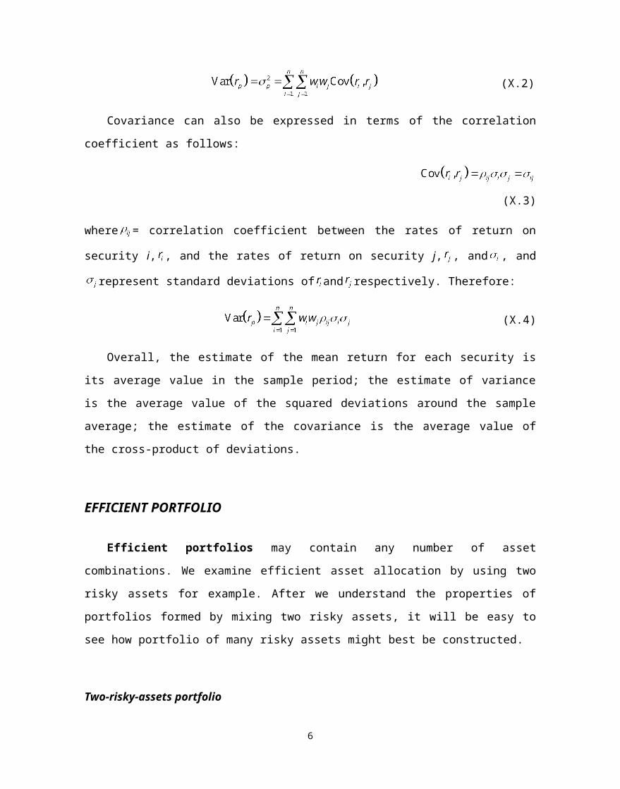
Overall, the estimate of the mean return for each security is its average value in the sample

period; the estimate of variance is the average value of the squared deviations around the sample

average; the estimate of the covariance is the average value of the cross-product of deviations.

EFFICIENT PORTFOLIO

Efficient portfolios may contain any number of asset combinations. We examine efficient

asset allocation by using two risky assets for example. After we understand the properties of

portfolios formed by mixing two risky assets, it will be easy to see how portfolio of many risky

assets might best be constructed.

Two-risky-assets portfolio

Because we now envision forming a -portfolio from two risky assets, we need to understand how

the uncertainties of asset returns interact. It turns out that the key determinant of portfolio risk id the

extent to which the returns on the two assets tend to vary rather in tandem or in opposition. The

degree to which a two-risky-assets portfolio reduces variance of returns depends on the degree of

correlation between the returns of the securities.

Suppose a proportion denoted by is invested in asset A, and the remainder , denoted by

, is invested in asset B. The expected rate of return on the portfolio is a weighted average of the

expected returns on the component assets, with the same portfolio proportions as weights.

(X.5)

The variance of the rate of return on the two-asset portfolio is

(X.6)

where is the correlation coefficient between the returns on asset A and asset B. If the

correlation between the component assets is small or negative, this will reduce portfolio risk.

First, assume that , which would mean that Asset A and B are perfectly positively

correlated, the right-hand side of equation X.6 is a perfect square and simplifies to

5

or

Therefore, the portfolio standard deviation is a weighted average of the component security

standard deviations only in the special case of perfect positive correlation. In this circumstance,

there are no gains to be had form diversification. Whatever the proportions of asset A and asset B,

both the portfolio mean and the standard deviation are simple weighted averages. Figure X.1 shows

the opportunity set with perfect positive correlation - a straight line through the component assets.

No portfolio can be discarded as inefficient in this case, and the choice among portfolios depends

only on risk preference. Diversification in the case of perfect positive correlation is not effective.

Figure X.1 Investment opportunity sets for asset A and asset B with various correlation coefficients3

Perfect positive correlation is the only case in which there is no benefit from diversification.

With any correlation coefficient less than 1.0( ), there will be a diversification effect, the

portfolio standard deviation is less than the weighted average of the standard deviations of the

component securities. Therefore, there are benefits to diversification whenever asset returns are less

than perfectly correlated.

Our analysis has ranged from very attractive diversification benefits ( ) to no benefits at

all . For within this range, the benefits will be somewhere in between.

Negative correlation between a pair of assets is also possible. Where negative correlation is

3 The proofs of the slope and the shape of extreme correlation between asset A and asset B are in Appendix A.

0 Standard Deviation

Exp

ecte

d R

etur

n

asset B

asset A

1

0 1

0 1

1

6

present, there will be even greater diversification benefits. Again, let us start with an extreme. With

perfect negative correlation, we substitute in equation X.6 and simplify it in the same

way as with positive perfect correlation. Here, too, we can complete the square, this time, however,

with different results.

And, therefore,

(X.7)

With perfect negative correlation, the benefits from diversification stretch to the limit.

Equation X.7 points to the proportions that will reduce the portfolio standard deviation all the way

to zero.

An investor can reduce portfolio risk simply by holding instruments which are not perfectly

correlated. In other words, investors can reduce their exposure to individual asset risk by holding a

diversified portfolio of assets. Diversification will allow for the same portfolio return with reduced

risk.

The concept of Markowitz efficient frontier

Every possible asset combination can be plotted in risk-return space, and the collection of all

such possible portfolios defines a region in this space. The line along the upper edge of this region

is known as the efficient frontier. Combinations along this line represent portfolios (explicitly

excluding the risk-free alternative) for which there is lowest risk for a given level of return.

Conversely, for a given amount of risk, the portfolio lying on the efficient frontier represents the

combination offering the best possible return. Mathematically the efficient frontier is the

intersection of the set of portfolios with minimum variance and the set of portfolios with maximum

return.

Figure X.2 shows investors the entire investment opportunity set, which is the set of all

attainable combinations of risk and return offered by portfolios formed by asset A and asset B in

differing proportions. The curve passing through A and B shows the risk-return combinations of all

the portfolios that can be formed by combining those two assets. Investors desire portfolios that lie

to the northwest in Figure X.2. These are portfolios with high expected returns (toward the north of

the figure) and low volatility (to the west).

7

Figure X.2 Investment opportunity set for asset A and asset B

The area within curve BVAZ is the feasible opportunity set representing all possible portfolio

combinations. Portfolios that lie below the minimum-variance portfolio (point V) on the figure can

therefore be rejected out of hand as inefficient. The portfolios that lie on the frontier VA in Figure

X.2would not be likely candidates for investors to hold. Because they do not meet the criteria of

maximizing expected return for a given level of risk or minimizing risk for a given level of return.

This is easily seen by comparing the portfolio represented by points B and B’. Since investors

always prefer more expected return than less for a given level of risk, B’ is always better than B.

Using similar reasoning, investors would always prefer B to V because it has both a higher return

and a lower level of risk. In fact, the portfolio at point V is identified as the minimum-variance

portfolio; since no other portfolio exists that has a lower standard deviation. The curve VA

represents all possible efficient portfolios and is the efficient frontier4, which represents the set of

portfolios that offers the highest possible expected rate of return for each level of portfolio standard

deviation.

4 The efficient frontier will be convex – this is because the risk-return characteristics of a portfolio change in a non-linear fashion as its component weightings are changed. (As described above, portfolio risk is a function of the correlation of the component assets, and thus changes in a non-linear fashion as the weighting of component assets changes.) The efficient frontier is a parabola (hyperbola) when expected return is plotted against variance (standard deviation).

A

Minimum Variance Portfolio (MVP)

0

B

B’

InvestmentOpportunitySet

V

Standard Deviation

Exp

ecte

d R

etur

n

Z

8

Figure X.3 The efficient frontier of risky assets and individual assets

Any portfolio on the down ward sloping potion of the frontier curve is dominated by the

portfolio that lies directly above it on the upward sloping portion of the frontier curve since that

portfolio has higher expected return and equal standard deviation. The best choice among the

portfolios on the upward sloping portion of the frontier curve is not as obvious, because in this

region higher expected return is accompanied by higher risk. The best choice will depend on the

investor’s willingness to trade off risk against expected return.

Short selling

Various constraints may preclude a particular investor from choosing portfolios on the efficient

frontier, however. Short sale restrictions are only one possible constraint. Short sale is a usual

regulated type of market transaction. It involves selling assets that are borrowed in expectation of a

fall in the assets’ price. When and if the price declines, the investor buys an equivalent number of

assets at the new lower price and returns to the lender the assets that was borrowed.

Now, relaxing the assumption of no short selling, investors could sell the lowest-return asset B

(here, we assume that ). If the number of short sales is unrestricted,

then by a continuous short selling of B and reinvesting in A the investor could generate an infinite

expected return. The efficient frontier of unconstraint portfolio is shown in Figure X.4. The upper

bound of the highest-return portfolio would no longer be A but infinity (shown by the arrow on the

top of the efficient frontier). Likewise the investor could short sell the highest-return security A and

0

Efficient frontier of risky assets

Standard Deviation

Exp

ecte

d R

etur

n

Individual assets

Minimum variance portfolio

9

reinvest the proceeds into the lowest-yield security B5, thereby generating a return less than the

return on the lowest-return assets. Given no restriction on the amount of short selling, an infinitely

negative return can be achieved, thereby removing the lower bound of B on the efficient frontier.

Hence, short selling generally will increase the range of alternative investments from the minimum-

variance portfolio to plus or minus infinity6.

Figure X.4 The efficient frontier of unrestricted/restricted portfolio

Relaxing the assumption of no short selling in this development of the efficient frontier

involves a modification of the analysis of the efficient frontier of constraint (not allowed short

sales). Next section, we introduce the mathematical analysis of the efficient frontier with/without

short selling constraints.

Calculating the Minimum variance portfolio

In Markowitz portfolio model, we assume investors choose portfolios based on both expected

return, , and the standard deviation of return as a measure of its risk, . So, the portfolio

selection problem can be expressed as maximizing the return with respect to the risk of the

investment (or, alternatively, minimizing the risk with respect to a given return, hold the return

constant and solve for the weighting factors that minimize the variance).

5 Rational investor will not short sell a high-return asset and buy a low-return asset. This case is just for extreme assumption.6 Whether an investor engages in any of this short-selling activity depends on the investor’s own unique set of indifference curves.

0

Z’

Z

A

P

V

Exp

ecte

d R

etur

n

Standard Deviation

B

without short saleswith short sales

10

Mathematically, the portfolio selection problem can be formulated as quadratic program. For

two risky assets A and B, the portfolio consists of , the return of the portfolio is then, The

weights should be chosen so that (for example) the risk is minimized, that is

for each chosen return and subject to . The last two constraints

simply imply that the assets cannot be in short positions.

The minimum variance portfolio weights are shown in Table X.1, the detail proofs are in

Appendix B.

Table X.1 The mimimum variance portfolio weight of two-assets portfolio without short selling

The correlation of two assets Weight of Asset A Weight of Asset B

ρ= 1

ρ= -1

ρ= 0

Above, we simply use two-risky-assets portfolio to calculate the minimum variance portfolio

weights. If we generalization to portfolios containing assets, the minimum portfolio weights can

then be obtained by minimizing the Lagrange function C for portfolio variance.

(X.8)

in which are the Lagrange multipliers, respectively, is the correlation coefficient between

and , and other variables are as previously defined.

By using this approach the minimum variance can be computed for any given level of expected

portfolio return (subject to the other constraint that the weights sum to one). In practice it is best to

11

use a computer because of the explosive increase in the number of calculations as the number of

securities considered grows. The efficient set that is generated by the aforementioned approach

(equation X.8) is sometimes called the minimum-variance set because of the minimizing nature of

the Lagrangian solution.

Calculating the weights of optimal risky portfolio

One of the goals of portfolio analysis is minimizing the risk or variance of the portfolio.

Previous section introduce the calculation of minimum variance portfolio, we minimum the

variance of portfolio subject to the portfolio weights’ summing to one. If we add a condition into

the equation X.8, whish is be subject to the portfolio’s attaining some target expected rate of

return, we can get the optimal risky portfolio.

Subject to

, where is the target expected return and

The first constraint simply says that the expected return on the portfolio should equal the target

return determined by the portfolio manager. The second constraint says that the weights of the

securities invested in the portfolio must sum to one.

The Lagrangian objective function can be written:

(X.9)

Taking the partial derivatives of this equation with respect to each of the variables,

and setting the resulting equations equal to zero yields the minimization of risk

subject to the Lagrangian constraints. Then, we can solve the weights and these weights are

represented optimal risky portfolio by using of matrix algebra.

If there no short selling constraint in the portfolio analysis, second constraint, , should

12

substitute to , where the absolute value of the weights allows for a given to be

negative (sold short) but maintains the requirement that all funds are invested or their sum equals

one.

The Lagrangian function is

(X.10)

If the restriction of no short selling is in minimization variance problem, it needs to add a third

constraint:

The addition of this non-negativity constraint precludes negative values for the weights (that

is, no short selling). The problem now is a quadratic programming problem similar to the ones

solved so far, except that the optimal portfolio may fall in an unfeasible region. In this circumstance

the next best optimal portfolio is elected that meets all of the constraints.

Finding the efficient frontier of risky assets

According to two-fund separation, the efficient frontier of risky assets can be formed by any

two risky portfolios one the frontier. All portfolios on the mean-variance efficient frontier can be

formed as a weighted average of any two portfolios or funds on the efficient frontier , is called two-

fund separation. So if we have any two points of the portfolio combinations, we can draw an entire

efficient frontier of the risky assets. Previous sections we have introduced the minimum variance

portfolio and optimal risky portfolio given the expected return, then, we can generate the entire

efficient frontier by the separation property.

Deriving the efficient frontier may be quite difficult conceptually, but computing and graphing it

with any number of assets and any set of constraints is quite straightforward. Later, we will use

EXCEL and MATLAB to generate the efficient frontier.

Finding the optimal risky portfolio

We already have an efficient frontier, however, how we deicide the best allocation of portfolio?

One of the factors to consider when selecting the optimal portfolio for a particular investor is degree

13

of risk aversion, investor’s willingness to trade off risk against expected return. This level of

aversion to risk can be characterized by defining the investor’s indifference curve, consisting of the

family of risk/return pairs defining the trade-off between the expected return and the risk. It

establishes the increment in return that a particular investor will require in order to make an

increment in risk worthwhile. The optimal portfolio along the efficient frontier is not unique with

this model and depends upon the risk/return tradeoff utility function of each investor. We use the

utility function that is commonly employed by financial theorists and the AIMR (Association of

Investment Management and Research) assigns a portfolio with a given expected return and

standard deviation the following utility function:

(X.11)

where is the utility value and A is an index of the investor’s risk aversion. The factor of 0.005 is

a scaling convention that allows us to express the expected return and standard deviation in

equation X.11 as percentages rather than decimals. We interpret this expression to say that the

utility from a portfolio increases as the expected rate of return increases, and it decreases when the

variance increases. The relative magnitude of these changes is governed by the coefficient of risk

aversion, A . For risk-neutral investors, A=0. Higher levels of risk aversion are reflected in larger

values for A.

Portfolio selection, then, is determined by plotting investors’ utility functions together with the

efficient-frontier set of available investment opportunities. In Figure X.6, two sets of indifference

curves labeled and are shown together with the efficient frontier. The curve has a higher

slope, indicating a greater level of risk aversion. The investor is indifferent to any combination of

and along a given curve. The curve would be appropriate for a less risk-averse investor—that

is, one who would be willing to accept relatively higher risk to obtain higher levels of return. The

optimal portfolio would be the one that provides the highest utility—a point in the northwest

direction (higher return and lower risk). This point will be at the tangent of a utility curve and the

efficient frontier. Each investor is logically selecting the optimal portfolio given his or her risk-

return preference, and neither is more correct than the other.

14

Figure X.6 Indifference Curves and Efficient frontier

In order to simplify the determination of optimal risky portfolio, we use the capital allocation

line (CAL), which depicts all feasible risk-return combinations available from different asset

allocation choices, to determine the optimal risky portfolio. To start, however, we will demonstrate

the solution of the portfolio construction problem with only two risky assets (in our example, asset

A and asset B) and a risk-free asset. In this case, we can derive an explicit formula for the weights

of each asset in the optimal portfolio. This will make it easy to illustrate some of the general issues

pertaining to portfolio optimization.

The objective is to find the weights and that result in the highest slope of the CAL

( i.e., the weights that result in the risky portfolio with the highest reward-to-variability ratio).

Therefore, the objective is to maximize the slope of the CAL for any possible portfolio, P. Thus out

objective function is the slope that we have called : The entire portfolio including risky and

risk-free assets.

(X.12)

For the portfolio with two risky assets, the expected return and standard deviation of portfolio

S are

(X.5)

0

BA

Standard Deviation

Exp

ecte

d R

etur

n

Minimum variance portfolio Efficient

frontier ofrisky assets

1U

2U

15

(X.13)

When we maximize the objection function, , we have to satisfy the constraint that the

portfolio weights sum to 1. Therefore, we solve a mathematical problem formally written as

Subject to .In this case of two risky assets, the solution for the weights of the optimal

risky portfolio S, can be shown to be as follows7:

Then, we form an optimal complete portfolio8 given an optimal risky portfolio and the CAL

generated by a combination of portfolio S and risk-free asset. We have constructed the optimal

portfolio S, we can use the individual investor’s degree of risk aversion, A, to calculate the optimal

proportion of complete portfolio to invest in the risky component.

Assuming that a risk-free rate is , and a risky portfolio with expected return and

standard deviation will find that, for any choice of , the expected return of the complete

portfolio is

The variance of the overall portfolio is

The investor attempts to maximum utility, U, by choosing the best allocation to the risky asset,

. To solve the utility maximization problem more generally, we write the problem as follows:

7 The solution procedure for two risky assets is as follows. Substitute for expected return from equationX.5 and for standard deviation from equation X.13. Substitute for . Differentiate the resulting expression for Sp with

respect to , set the derivative equal to zero, and solve for .8 The complete portfolio means that the entire portfolio including risky and risk-free assets.

16

Setting the derivative of this expression to zero, we can solve for yield the optimal position

for risk-averse investors in the risky asset, , as follows:

(X.14)

The solution shows that the optimal position in the risky asset is, as one would expect,

inversely proportional to the level of risk aversion and the level of risk (measured by the variance)

and directly proportional to the risk premium offered by the risky asset.

Once we have reached this point, generalizing to the case of many risky assets is

straightforward. Before we move on, let us briefly summarize the steps we followed to arrive at the

complete portfolio.

1. Specify the return characteristics of all securities (expected returns, variances,

covariances).

2. Establish the risky portfolio:

a. Calculate the optimal risky portfolio S.

b. Calculate the properties of portfolio S using the weights determined in step and

equations X.5 and X.13.

3. Allocation funds between the risky portfolio and the risk-free asset:

a. Calculate the fraction of the complete portfolio allocated to Portfolio S (the risky

portfolio) and to risk-free asset (equation X.14).

b. Calculate the share of the complete portfolio invested in each asset and in risk-free

asset.

17

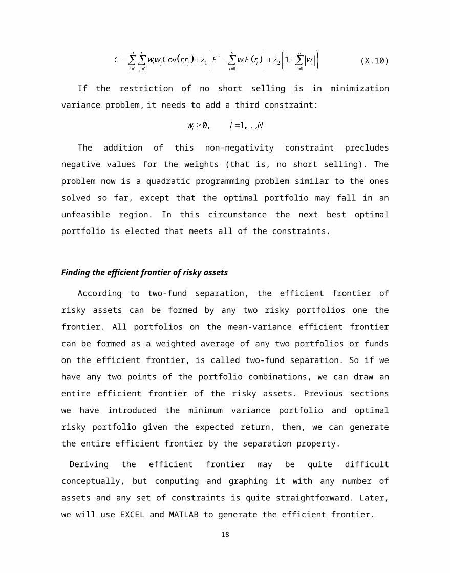
Figure X.7 Determination of the optimal portfolio

In practice, when we try to construct optimal risky portfolios from more than two risky assets

we need to rely on Microsoft EXCEL or another computer program. We present can be used to

construct efficient portfolios of many assets in the next section.

ALTERNATIVE COMPUTER PROGAME TO CALCULATE EFFICIENT FRONTIER

Several software packages can be used to generate the efficient frontier. In this section, we will

demonstrate the method using Microsoft Excel and MATLAB.

Application: Microsoft Excel

Excel is far from the best program for generating the efficient frontier and is limited in the

number of assets it can handle, but working through a simple portfolio optimizer in Excel can

illustrate concretely the nature of the calculations used in more sophisticated ‘black-box’ programs.

You will find that Excel, the computation o the efficient frontier is fairly easy.

Assume an American investor who forms a six-stock-index portfolio. The portfolio consists of

six stock indexes: United State (S&P500), United Kingdom (FTSE100), Switzerlan (Swiss Market

Index, SMI) ,Singapore (Straits Times Index, STI), HongKong (Hang Seng Index, HSI) , and Korea

(Korea Composite Stock Price Index, KOSPI), with monthly price data from Jan. 1990 to Dec.

2006. He/she wants to know his/her optimal portfolio allocation.

Indifference CurveOpportunity Set of Risky Assets

Optimal CompletePortfolio

CAL

0

Optimal Risky Portfolio

Standard Deviation

Exp

ecte

d R

etur

n

fr

18

The Markowitz portfolio selection problem can be divided into three parts. First, we need to

calculate the efficient frontier. Secondly, we need to choose the optimal risky portfolio given one’s

capital allocation line (find the point at the tangent of a CAL and the efficient frontier). Finally,

using the optimal complete portfolio allocate funds between the risky portfolio and the risk-free

asset.

Step one: Finding efficient frontier

First, we need to calculate expected return, standard deviation, and covariance matrix. The

expected return and standard deviation can been calculated by applying the Excel STDEV and

AVERAGE functions to the historic monthly percentage returns data9. Table X.2A and B shows

average returns, standard deviations, and the correlation matrix10 for the rates of return on the stock

index. After we input Table X.2A into our spreadsheet as shown, we create the covariance matrix in

Table X.2B using the relationship .

Table X.2 Performance of six stock indexes

9 The expected return and standard deviation of each index need to be annualized.10 The correlation matrix is calculated in Excel using the data analysis function that is found under the Tool Menu. Note if Data Analysis does not appear on the Tool Menu you will need to select Add-in and add to the Menu.

19

Table X.2 (Concluded)

20

Table X.2 (Concluded)

21

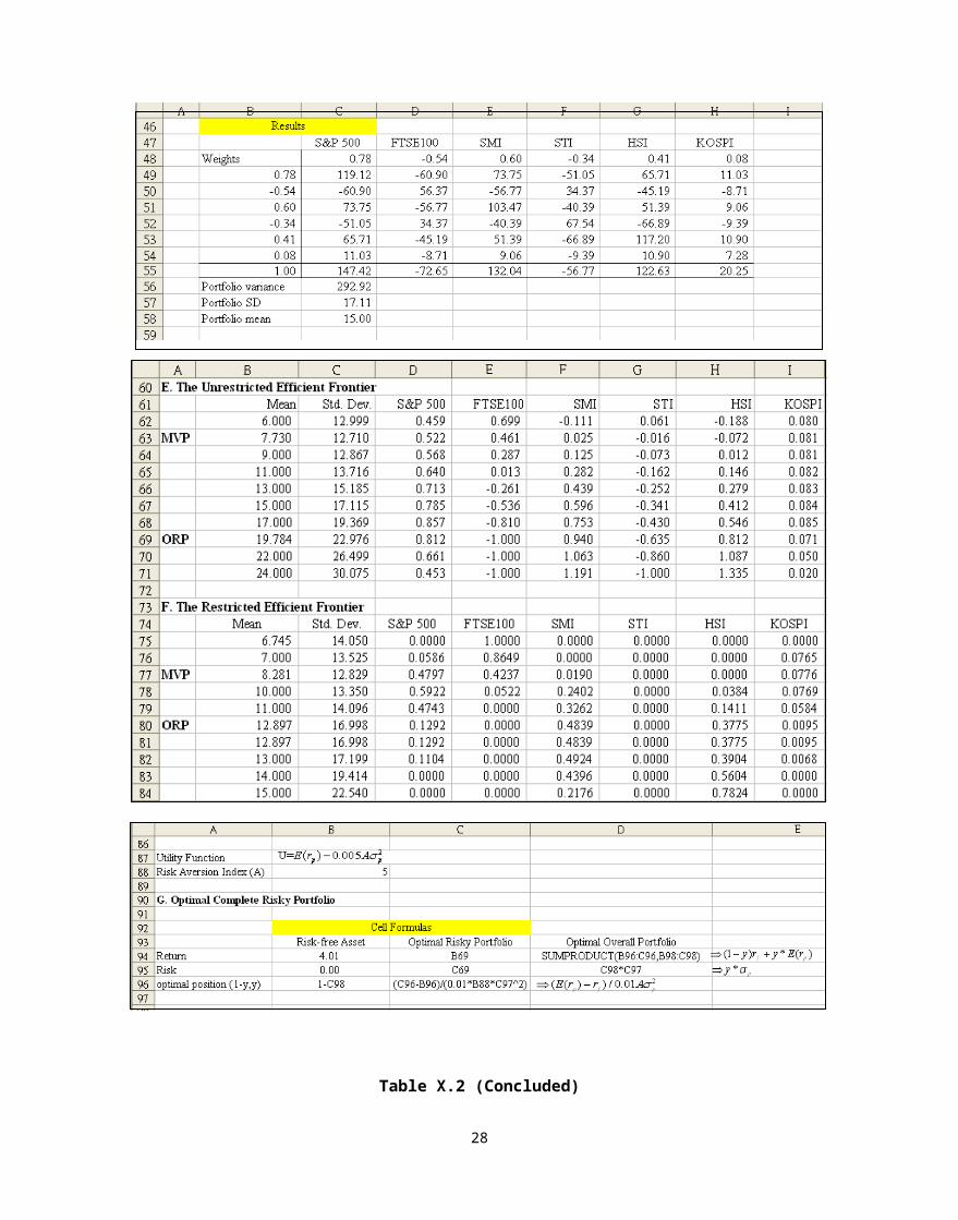
Before computing of the efficient frontier, we need to prepare the data to establish a

benchmark against which to evaluate our efficient portfolios, we can form a border-multiplied

covariance matrix. We use the target mean of 15% for example. To compute the target portfolio’s

mean and variance, these weights are entered in the border column B49-B54 and border row C48-

H48. We calculate the variance of this portfolio in cell C56 in Table X.2D. The entry in C56 equals

the sum of all elements in the border-multiplied covariance matrix where each element is first

multiplied by the portfolio weights given in both the row and column borders. We also include two

cells to compute the standard deviation and expected return of the target portfolio (formulas in cells

C57, C58)11.

To compute points along the efficient frontier we use the Excel Solver in Table X.2D (which you

can find in the Tools menu)12. Once you bring up Solver, you are asked to enter the cell of the target

(objective) function. In our application, the target is the variance of the portfolio, given in cell C56.

Solver will minimize this target. You next must input the cell range if the decision variables ( in this

case, the portfolio weights, contained in cells B49-B54). Finally, you enter all necessary constraints

into the Solver. For an unrestricted efficient frontier that allows short sales, there are two

constraints: first, that the sum of the weights1.0 (cell B55=1), and second, that the portfolio

expected return equals target return 15% (cell B58=15)13. Once you have entered the two

constraints you ask the Solver to find the optimal portfolio weights.

The Solver beeps when it has found a solution and automatically alters the portfolio weight

cells in row 48 and column C to show the makeup of the efficient portfolio. It adjusts the entries in

the border-multiplied covariance matrix to reflect the multiplication by these new weights, and it

shows the mean and variance of this optimal portfolio-the minimum variance portfolio with mean

return of 15%. These results are shown in Table X.2D, cells C56-C58. You can find that they yield

an expected return of 15% with a standard deviation of 17.11% (results in cells C58 and C57). To

generate the entire efficient frontier, keep changing the required mean in the constraint (cell C58),

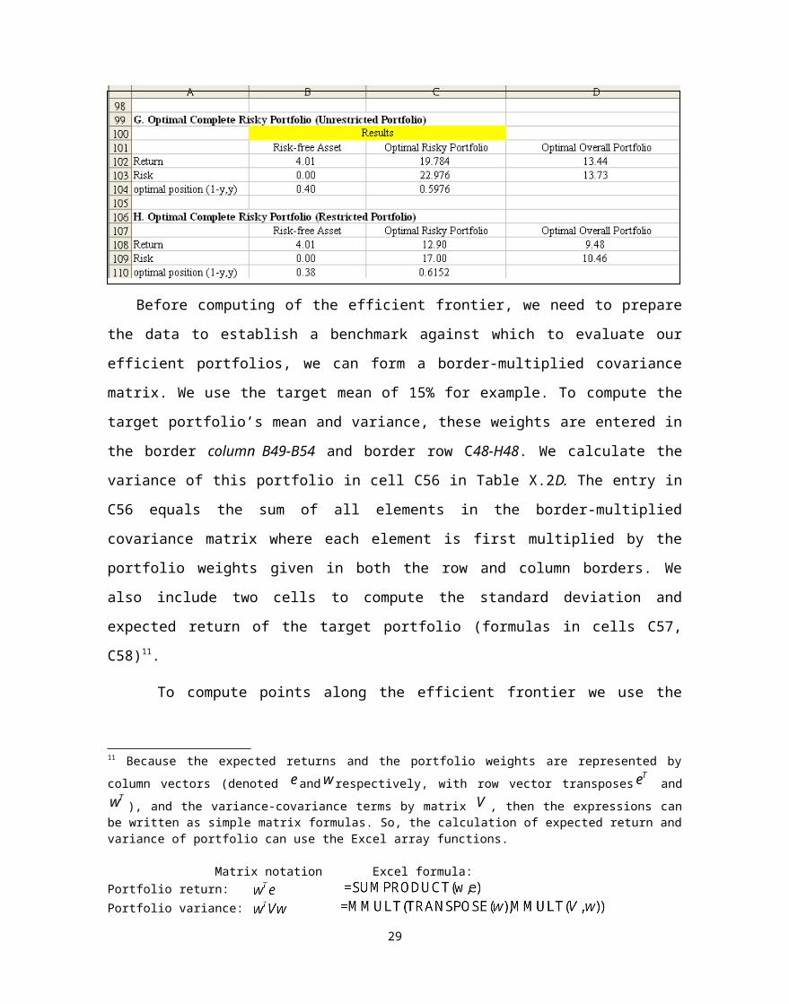
11 Because the expected returns and the portfolio weights are represented by column vectors (denoted e and w

respectively, with row vector transposesTe and

Tw ), and the variance-covariance terms by matrix V , then the expressions can be written as simple matrix formulas. So, the calculation of expected return and variance of portfolio can use the Excel array functions.

Matrix notation Excel formula: Portfolio return: Portfolio variance: 12 If Solver does not show up under the Tools menu, you should select Add-Ins and then select Analysis. This should ass Solver to the list of options in the Tools menu.13 If you do not set the second constraint: target mean equal to 20, then you can the minimum variance portfolio. The minimum variance portfolio has 18.637% expected return and a standard deviation of 15.643%.

22

letting the Solver work for you. If you record a sufficient number of points, you will be able to

generate a graph of the quality of Figure X.8.

If short selling is not allowed, the Solver also allows you to all “no short sales” and other

constrains easily. We need to impose the additional constraints that each weight (the elements in

column B and row 49) must be nonnegative. Once they are entered, you repeat the variance-

minimization exercise until you generate the entire restricted frontier. The outer frontier in Figure

X.8 is drawn assuming that the investor may maintain negative portfolio weights, the inside frontier

obtained allowing short sales. Table X.2 E and F present a number of points on the two frontiers

with and without short sales. You can see that the weights in restricted portfolios are never negative.

The minimum variance portfolios in two frontiers are not the same.

Before we move on, let us summarize the steps of using Solver to calculate the variance-

minimization portfolio.

The steps with Solver are:

1. Invoke Solver by choosing Tools then Options then Solver.

2. Specify in the Solver parameter Dialog Box: the Target cell to be optimized specify max

or min

3. Choose Add to specify the constrains then OK

4. Solve and get the results in the spreadsheet.

Figure X.8 Efficient frontier of unrestricted and restricted portfolio

23

Step two: Finding optimal risky portfolio

Now that we have the efficient frontier, we proceed to step two. In order to get the optimal risky

portfolio, we should find the portfolio on the tangency point of capital allocation and efficient

frontier. To do so, we can use the Solver to help us. First, you enter the of the target function,

“maximum” the reward-to-variability ratio ( ,we assume risk-free rate is 4.01%14) the

slope of the CAL, input the cell range (the portfolio weights, contained in cells B49-B54), and other

necessary constraints( such like the sum of the weights equal to one and others). Then ask the

Solver to find the optimal portfolio weights. The results are shown in Table X.2 E and F. The

optimal risky portfolio with short selling allowance has expected return of 19.784% with a standard

deviation of 22.976% (cell B69, C69). The expected return and standard deviation of the restricted

optimal risky portfolio are 12.897%and 16.998% (cell B80, C80).

Step three: Capital allocation decision

One’s allocation decision will influence by his degree of risk aversion. Now we have optimal

risky portfolio, we can use the concept of complete portfolio allocation funds between risky

portfolio and risk-free asset. We use equation X.11 as our utility function and set the risk aversion

equal to 5 and risk-free rate is 4.1%. First we construct a complete portfolio with risk-free asset and

optimal risky portfolio.

14 We use three month Treasury Bill interest rate as the risk-free rate, the average interest rate of 3month T-Bill is 4.09% form 1990/01 to 2006/12.

24

According to equation X.14, the optimal weight in risky portfolio is and the optimal

position of risk-free asset is 1- . Then we can use equation 5 and 6 calculate the expected

return and standard deviation of the overall optimal portfolio. The results are shown in Table X.2 G

and H. The optimal unrestricted (restricted) portfolio has 13.44% (9.48%) expected return with

13.73% (10.46%) standard deviation. And the investor will invest 60% (62%) of portfolio value in

risky portfolio and 40% (38%) in risk-free asset.

To sum up the three steps, the all results are shown in Table X.3.

Table X.3 The results of optimization problem

portfolio Unrestricted portfolio Restricted portfolioMinimum variance portfolio

Optimal risky

portfolio

OptimalOverall portfolio

Minimum variance portfolio

Optimal risky

portfolio

OptimalOverall portfolio

Portfolio Return 7.73% 19.78% 13.44% 8.28% 12.89% 9.48%

Portfolio Risk 12.71% 22.98% 13.73% 12.83% 16.99% 10.46%

Application: MATLAB

By using the Solve, you can repeat the variance-minimization exercise until you generate the

entire efficient frontier, just with on push of a button. The computation of the efficient frontier is

fairly easy in Microsoft Excel. However, Excel is limited in the number of assets it can handle. If

our portfolio consists of hundreds of asset, using Excel to deal with the Markowitz optimal problem

will become more complicated. MATLAB can handle this problem. The Financial Toolbox in

MATLAB provides a complete integrated computing environment for financial analysis and

engineering. The toolbox has everything you need to perform mathematical and statistical analysis

of financial data and display the results with presentation-quality graphics. You do not need to

switch tools, convert files, or rewrite applications. Just write expressions the way you think of

problems, MATLAB will do all that for you. You can quickly ask, visualize, and answer

complicated questions.

Financial Toolbox includes a set of portfolio optimization functions designed to find the portfolio

that best meets investor requirements. Recall the steps when using Excel in previous section. In the

portfolio optimization problem, we need to prepare several the data for the computation preparation.

25

First, we need the expected return, standard deviation, covariance matrix. Then, we can calculate

the optimal risky portfolio weights and know how allocate will be more efficient. Before taking real

portfolio selection example by using MATLAB, we introduce the several portfolio optimization

functions that will be use in our portfolio selection analysis.

Mean-variance efficient frontier

Calling function frontcon can returns the mean-variance efficient frontier for a given group

of assets with user-specified asset constraints, covariance, and returns. The computation is based on

sets of constraints representing the maximum and minimum weights for each asset, and the

maximum and minimum total weight for specified groups of assets. The efficient frontier

computation functions require information about each asset in the portfolio. This data is entered into

the function via two matrices: an expected return vector and a covariance matrix. Calling

frontcon while specifying the output arguments returns the corresponding vectors and arrays

representing the risk, return, and weights for each of the 10 points computed along the efficient

frontier. Since there are no constraints, you can call frontcon directly with the data you already

have. If you call frontcon without specifying any output arguments, you get a graph representing

the efficient frontier curve.

Function: frontcon

Syntax[PortRisk, PortReturn, PortWts] = frontcon(ExpReturn, ExpCovariance, NumPorts,

PortReturn, AssetBounds, Groups,

GroupBounds)

PortRisk, PortReturn and PortWts are the returns of frontcon, where PortRisk is a

vector of the standard deviation of each portfolio, PortReturn is a vector of the expected return

of each portfolio, and PortWts is an matrix of weights allocated to each asset15. The output data is

represented row-wise, where each portfolio’s risk, rate of return, and associated weight is identified

as corresponding rows in the vectors and matrix.

ExpReturn, ExpCovariance, NumPorts are frontcon required information, NumPorts,

PortReturn, AssetBounds , and GroupBounds all are optional information. ExpReturn

specifies the expected return of each asset; ExpCovariance specifies the covariance of the asset

returns. PortWts is a he matrix of weights allocated to each asset, an optional item. In

15 The total of all weights in a portfolio is 1.

26

NumPorts, you can define the number of portfolios you want to be generated along the efficient

frontier. If NumPorts is empty (entered as []), frontcon computes 10 equally spaced points16.

PortReturn is vector of length equal to the number of portfolios containing the target return

values on the frontier. If PortReturn is not entered or [], NumPorts equally spaced returns

between the minimum and maximum possible values are used. AssetBounds is a matrix

containing the lower and upper bounds on the weight allocated to each asset in the portfolio17.

Groups is number of groups matrix specifying asset groups or classes18. GroupBounds matrix

allows you to specify an upper and lower bound for each group. Each row in this matrix represents

a group. The first column represents the minimum allocation, and the second column represents the

maximum allocation to each group.

Notice, the arguments in the parentheses are the function required data; the items in the square

bracket are the returns of function, the return will be show in the output. If you do not want to

results show up in output window, you can clear the square bracket just keep the item. On the

contrary, if you want show some results in the output window, just add square bracket when

expression feedback of functions in writing syntax. Moreover, the names of input arguments can be

user-specified, it is not necessary to be named as our example shown. You can name what you want,

as long as the concept of data matches the function arguments required.

Portfolios on constrained efficient frontier

If you want set some linear constraints when computing efficient frontier, you can call

portopt function. The portopt computes portfolios along the efficient frontier for a given

group of assets, based on a set of user-specified linear constraints. Typically, these constraints are

generated using the constraint specification functions which we will describe in next section.

Function: portopt

Syntax [PortRisk, PortReturn, PortWts] = portopt(ExpReturn, ExpCovariance, NumPorts,

PortReturn, ConSet)

The portopt is an advanced version of frontcon function. The most difference between

this two is ConSet, others are the same as our described in frontcon function. ConSet, optional

16 When entering a target rate of return (PortReturn), enter NumPorts as an empty matrix [].17 The Default of lower asset bound is all 0s (no short-selling); default upper asset bound is all 1s (any asset may constitute the entire portfolio).18 Groups(i,j) = 1 (jth asset belongs in the ith group). Groups(i,j) = 0 (jth asset not a member of the ith group).

27

information, is a constraint matrix for a portfolio of asset investments, created using portcons. If

not specified, a default is created. The syntax expressed above will return the mean-variance

efficient frontier with user-specified covariance, returns, and asset constraints (ConSet). If

portopt is invoked without output arguments, it returns a plot of the efficient frontier.

Portfolio constraints

While frontcon allows you to enter a fixed set of constraints related to minimum and

maximum values for groups and individual assets, you often need to specify a larger and more

general set of constraints when finding the optimal risky portfolio. The function portopt addresses

this need, by maccepting an arbitrary set of constraints as an input matrix. The auxiliary function

portcons can be used to create the matrix of constraints, with each row representing an inequality.

These inequalities are of the type A*Wts' <= b, where A is a matrix, b is a vector, and Wts is a row

vector of asset allocations. The number of columns of the matrix A, and the length of the vector

Wts correspond to the number of assets. The number of rows of the matrix A, and the length of

vector b correspond to the number of constraints. This method allows you to specify any number of

linear inequalities to the function portopt19.

Function: portcons

Syntax

ConSet = portcons(varargin20)

ConSet = portcons('ConstType', Data1, ..., DataN) creates a matrix ConSet, based on

the constraint type ConstType, and the constraint parameters Data1, ..., DataN.

ConSet = portcons('ConstType1', Data11, ..., Data1N,'ConstType2', Data21, ...,

Data2N, ...) creates a matrix ConSet, based on the constraint types ConstTypeN, and the

corresponding constraint parameters DataN1, ..., DataNN.

Table X.4 The detail information of portcons function

19 In reality, portcons is an entry point to a set of functions that generate matrices for specific types of constraints. portcons allows you to specify all the constraints data at once, while the specific portfolio constraint functions allow you to build the constraints incrementally. These constraint functions are pcpval, pcalims, pcglims, and pcgcomp.20 varargin is variable length input argument list. The varargin statement is used only inside a function M-file to contain optional input arguments passed to the function. The varargin argument must be declared as the last input argument to a function, collecting all the inputs from that point onwards. In the declaration, varargin must be lowercase.

28

Constraint type Description ValueDefault All allocations are >= 0; no

short selling allowed. Combined value of portfolio allocations normalized to 1

NumAssets (required). Scalar representing number of assets in portfolio.

PortValue Fix total value of portfolio to PVal.

PVal (required). Scalar representing total value of portfolio. NumAssets (required). Scalar representing number of assets in portfolio.

AssetLims Minimum and maximum allocation per asset.

AssetMin (required). Scalar or vector of length NASSETS, specifying minimum allocation per asset.AssetMax (required). Scalar or vector of length NASSETS, specifying maximum allocation per asset.NumAssets (optional).

GroupLims Minimum and maximum allocations to asset group.

Groups (required). NGROUPS-by-NASSETS matrix specifying which assets belong to each group.GroupMin (required). Scalar or a vector of length NGROUPS, specifying minimum combined allocations in each group.GroupMax (required). Scalar or a vector of length NGROUPS, specifying maximum combined allocations in each group.

GroupComparison Group-to-group comparison constraints.

GroupA (required). NGROUPS-by-NASSETS matrix specifying first group in the comparison.AtoBmin (required). Scalar or vector of length NGROUPS specifying minimum ratios of allocations in GroupA to allocations in GroupB.AtoBmax (required). Scalar or vector of length NGROUPS specifying maximum ratios of allocations in GroupA to allocations in GroupB.GroupB (required). NGROUPS-by-NASSETS matrix specifying second group in the comparison.

Custom Custom linear inequality constraints A*PortWts' <= b.

A (required). NCONSTRAINTS-by-NASSETS matrix, specifying weights for each asset in each inequality equation. b (required). Vector of length NCONSTRAINTS specifying the right hand sides of the inequalities.

Source: MATLAB Financial toolbox

Optimal capital allocation to efficient frontier portfolios

A last function we describe here may be used to find an optimal portfolio. So far, we have deal

29

with efficient portfolios, leaving the risk/return trade-off unresolved. We may resolve this trade-off

by linking mean-variance portfolio theory to the more general utility theory. Function portalloc computes the optimal risky portfolio on the efficient frontier, based on the risk-free rate, the borrowing rate, and the investor’s degree of risk aversion. Also generates the capital allocation line, which provides the optimal allocation of funds between the risky portfolio and the risk-free asset. In the

Financial toolbox the function portalloc is provided, which yields the optimal portfolio assuming

the quadratic utility function: , where the parameter A is linked to risk

aversion; its default value is 3.

Function: portalloc

Syntax

[RiskyRisk, RiskyReturn, RiskyWts, RiskyFraction, OverallRisk, OverallReturn]

= portalloc(PortRisk, PortReturn, PortWts, RisklessRate, BorrowRate,

RiskAversion)

RiskyRisk is the standard deviation of the optimal risky portfolio; RiskyReturn is the

expected return of the optimal risky portfolio; RiskyWts is a vector of weights allocated to the

optimal risky portfolio; RiskyFraction is the fraction of the complete portfolio allocated to the

risky portfolio; OverallRisk is the standard deviation of the optimal overall portfolio;

OverallReturn is the expected rate of return of the optimal overall portfolio.

PortRisk is standard deviation of each risky asset efficient frontier portfolio; PortReturn

is expected return of each risky asset efficient frontier portfolio; PortWts is weights allocated to

each asset. RisklessRate is risk-free lending rate (for investing), a decimal number;

BorrowRate is borrowing rate, which is larger than the riskless rate, a decimal number21.

RiskAversion is coefficient of investor's degree of risk aversion (Default = 3). BorrowRate and

RiskAversion are optional.

As with frontcon, calling portopt while specifying output arguments returns the

corresponding vectors and arrays representing the risk, return, and weights for each of the portfolios

along the efficient frontier. Use them as the first three input arguments to the function portalloc.

Calling portalloc while specifying the output arguments returns the variance (RiskyRisk), the

expected return (RiskyReturn), and the weights (RiskyWts) allocated to the optimal risky

21 If borrowing is not desired, or not an option, set to NaN (default).

30

portfolio. It also returns the fraction (RiskyFraction) of the complete portfolio allocated to the

risky portfolio, and the standard deviation (OverallRisk) and expected return (OverallReturn)

of the optimal overall portfolio consisting of the risky portfolio and the risk-free asset. The overall

portfolio combines investments in the risk-free asset and in the risky portfolio. The actual

proportion assigned to each of these two investments is determined by the degree of risk aversion

characterizing the investor. The value of RiskyFraction exceeds 1 (100%), implying that the risk

tolerance specified allows borrowing money to invest in the risky portfolio, and that no money will

be invested in the risk-free asset. This borrowed capital is added to the original capital available for

investment. Calling portalloc without specifying any output arguments gives a graph displaying

the critical points.

Six-stock-index portfolio

We use the previous example. Assume an American investor form six-stock-index portfolio and

he/she wants to what is his/her optimal portfolio allocation. We assume risk free investment return

is 4.1%, investor’s degree of risk aversion is 5, and borrowing rate is 7%. We also allow short

selling up to 100% of the portfolio value in each stock index, but limit the investment in any each

stock index to 150% of the portfolio value. Now we use MATLAB to assist him/her.

First, we calculate rate of return of the natural logarithm stock index price, save them as a text

file “ stock_index.txt ” into C:\ProgramFiles\MATLAB7\work\ stock_index.txt, and load this file

into MATLAB Secondly, use mean and cov functions calculate expected return of each stock index

and covariance matrix of portfolio. Thirdly, call portcons to create the matrix of constraints for

short selling allowance and call portfopt compute constrained efficient frontier. Then, Use

PortRisk, PortRet, PortWts input arguments to the function portalloc and find the optimal

risky portfolio and the optimal allocation of funds between the risky portfolio and the risk-free

asset.

31

Figure X.11 MATLAB code for asset allocationclear all;clc;tic%portfolio.mload stock_index.txt;Portfolio = stock_index (:,6);[m n] = size(Portfolio);[AvrRet]= mean(Portfolio);[ExpRetVec]= (1+ AvrRet).^12-1;[CovMtx]= cov(Portfolio);

% COMPUTE EFFICIENT FRONTIER (SHORT SELLING ALLOWED) NumPorts = n;AssetMin = [ -1 -1 -1 -1 -1 -1];AssetMax = [ 1.5 1.5 1.5 1.5 1.5 1.5];pval = 1;Constraint = portcons('PortValue',pval, NumPorts, 'AssetLims', AssetMin, AssetMax, NumPorts);[PortRisk,PortRet,PortWts] = portopt(ExpRetVec, CovMtx, 50, [], Constraint);[OptRisk,OptRet,OptWts]=portopt(ExpRetVec, CovMtx, NumPorts, [], Constraint);

% OPTIMAL ASSET ALLOCATIONRisklessRate = 0.041;BorrowRate = 0.07;RiskAversion = 5;[RiskyRisk, RiskyReturn, RiskyWts, RiskFraction, OverallRisk, OverallReturn] = portalloc (PortRisk, PortRet, PortWts, RisklessRate, BorrowRate, RiskAversion)

% PLOT THE RESULTplot(PortRisk, PortRet, 'm-', OptRisk, OptRet, 'x', ... 0, RisklessRate, 'k:square', RiskyRisk, RiskyReturn, 'k:diamond',... [0; RiskyRisk], [RisklessRate; RiskyReturn],'r--')xlabel('Portfolio Risk');ylabel('Portfolio Return ');title('Efficient Frontier');%legend('Efficient Frontier', 'Optimal Portfolio', 'Risk free asset', 'Risky Portfolio', 'Asset Allocation Point')

grid on

In this example the customer will tolerate borrowing 373.44% of the original capital amount to

invest in the six-stock-index portfolio, and that no money will be invested in the risk-free asset.

The optimal overall portfolio return is 84.28%with 39.31% standard deviation. The expected return

of six-stock-index portfolio is 23.32%, portfolio risk is 8.30%. The best allocation proportion of

each asset for the investor is to allocate 63.34% portfolio value in S&P 500 Index, 114.39% in

Swiss Market Index(SMI), and 122.93% in Hang Seng Index(HSI), and short selling 100%

portfolio value in FTSE100 Index, 94.45% in Straits Times Index(STI) ,and 6.21% in Korea

Composite Stock Price Index (KOPSI) .

32

Figure X.12 MATLAB output of optimal allocation problem

RiskyRisk =

0.0830

RiskyReturn =

0.2332

RiskyWts =

0.6334 -1.0000 1.1439 -0.9445 1.2293 -0.0621

RiskFraction =

4.7344

OverallRisk =

0.3931

OverallReturn =

0.8428

Figure X.13 Optimal asset allocation

33

ReferencesBenninga Simon, 1999, Financial Modeling, The MIT press, Combridge, Massachusetts, London,

England 1999.

Bodie Z., A. Kane ,and A. J. Marcus, 2003, Essentials of Investment, Fifth edition, xxxx:McGraw-

Hill.

Bodie Z., A. Kane ,and A. J. Marcus, 2005, Investment, Sixth edition, McGraw-Hill.

Brandimarte Paolo, Numerical Methods in Finance: A MATLAB-Based Introduction, New

York:John Wiley & Sons. Inc.

Cheng F. Lee, Joseph E. Finnerty, Donals H. Wort ,1990, Security Analysis and Portfolio

Management, xxxx:xxxx

Jackson Mary and Mike Staunton, 2002, Advanced Modelling in Finance using Excel and

VBA,xxxx:xxxx.

34

Appendix A

To prove the slope and the shape of extreme correlation between two assets

Assuming that the weight of asset A and asset B are , and .

Case one: Two assets are perfectly position correlated

If short sales are allowed, then even though

Selling short asset A and go extra long in asset B

35

Case Two: Two assets are perfectly negative correlated

Just invest both asset A and b (both in long position)

36

Appendix B

The weights of minimum variance portfolio

The weights should be chosen so that (for example) the risk is minimized, that is

for each chosen return and subject to . The last two constraints simply

imply that the assets cannot be in short positions.

Substitute into equation X.6.

F.O.C.

=

When ρ= 1

When ρ= -1

When ρ= 0

37