efficient numerical model for the damage detection of large scale structure

Engineering Structures 23 (2001) 436–451www.elsevier.com/locate/engstruct

Efficient numerical model for the damage detection of large scaleS.S. Law et al. /Engineering Structures 23 (2001) 436–451

S.S. Law*, T.H.T. Chan, D. WuDepartment of Civil and Structural Engineering, Hong Kong Polytechnic University, Hung Hom, Kowloon, Hong Kong

Received 19 October 1999; received in revised form and accepted 29 May 2000

Abstract

A structural modeling methodology is proposed, based on the concept of Damage-Detection-Orientated-Modeling, in which asuper-element representing a segment of a large-scale structure, e.g. a bridge deck, is developed. Each individual structural compo-nent is represented by a sub-element in the model. The large number of degrees-of-freedom in the analytical model is reduced,while the modal sensitivity relationship of the structural model to small physical changes is retained at the sub-element level. Theseproperties are significant to structural damage assessment. The concept of agenericsub-element is introduced in the parameterselection strategy for model updating, and the initial finite super-element model of the structure is updated using the eigensensitivitymethod. Numerical studies are presented to illustrate the super-element model and model updating method. Modal frequencies andthe mode shapes of the updated analytical models agree fairly well with the simulated measurements with or without noise andusing incomplete measurements with a maximum error of 12%. 2001 Elsevier Science Ltd. All rights reserved.

Keywords:Vibration; Large-scale structure; Generic element; Super-element; Model updating; Damage detection; Strain energy

1. Introduction

1.1. Structural modeling methodology

The initial finite element model of a modern civilengineering structure usually consists of a huge numberof degrees-of-freedom (DOF) from directly assemblingall the structural components. The number of the analyti-cal DOFs is generally much greater than the number ofincompletely measured DOFs. Direct comparisonbetween the information from the measured and the ana-lytical DOFs is not possible, and model reduction on theanalytical DOFs ([1]) or modal expansion on the meas-ured DOFs ([2]) are often employed to solve this prob-lem. However when the measured DOFs are far less thanthe analytical DOFs, both types of techniques will giverise to errors which would seriously degrade the accu-racy in further model updating and damage detectionprocedures. This may even results in an ill-posed inverseproblem. The latter is found in some extreme cases with

* Corresponding author. Tel.:+852-2766-6073; fax:+852-2334-6389.

0141-0296/01/$ - see front matter 2001 Elsevier Science Ltd. All rights reserved.PII: S0141-0296 (00)00066-3

a large dimension and many design variables, and wherea stable solution is not obtained.

To avoid the above-mentioned problems, efforts havebeen devoted to using reduced-order models for modelupdating and damage assessment. Stubbs et al. [3] pro-posed the equivalent continuum technique to detect con-struction errors in a large space structures. Kondo andHamamoto [4] extended the application of the techniqueto damage assessment, and they presented an improvedmethod to identify local damage in offshore platforms.However the equivalent continuum technique may maskthe behavior of individual members and bring aboutlarge modeling errors with the structural continuumassumption, so that the damage detection methods can-not always determine the specific structural componentthat is damaged in a space structure. The traditional sub-structuring technique ([5,6]) can also be used to decreasethe model dimension and reduce the system parameterto be updated. Since it is impossible to getprior knowl-edge of the damage region at the modeling stage, thedispersed substructures are required to be small enoughto localize and assess the structural damage accurately.Consequently, the model order and the number of systemparameters cannot be reduced reasonably. A more elab-

437S.S. Law et al. / Engineering Structures 23 (2001) 436–451

Nomenclature

[Kse] stiffness matrix of sub-elements[Mse] mass matrix of sub-elements[K] stiffness matrix of the structure[M] mass matrix of the structure[Fse] mode shape matrix of sub-elements[Lse] eigenvalue matrix (diagonal) of sub-elements[FR] rigid-body mode shape matrix of sub-elements[FS] strain mode shape matrix of sub-elements∂lr

∂pk eigenvalue sensitivity forrth mode∂{f} r

∂pk eigenvector sensitivities forrth mode∂[K]∂pk derivative of stiffness matrix with respect topk

∂[M]∂pk derivative of mass matrix with respect topk

∂[K sei ]

∂pk derivative of ith sub-element stiffness matrix with respect topk

∂[Msei ]

∂pk derivative of ith sub-element mass matrix with respect topk

pk the kth selected generic parameterli ith eigenvalue of sub-elements{f} i ith eigenvector of sub-elements(la)i ith eigenvalue of analytical model{fa} i ith eigenvector of analytical model(lx)r rth eigenvalue of experimental model{fx} r rth eigenvector of experimental model{ Dp} vector of generic parameter changesfA

ij element of analytical mode shape matrixfM

ij element of “measured” mode shape matrix[Si] generic transfer matrix inith updating iteration[Sn] updated transfer matrix aftern iterationsL number of sub-elements specified in super-element modelN number of DOFs specified in super-element modeln number of updating iterationsm number of “measured” (active) modesq number of calculated modesH number of selected generic parametersz number of DOFs specified in individual sub-element

orated modeling methodology is, therefore, needed fordamage assessment of modern civil engineering struc-tures.

Kim and Bartkowicz [7] tried to solve the problemwith a hybrid method in which the analytical DOFs arereduced to an intermediate number of DOFs whereas themeasured DOFs are expanded to match the reducedDOFs. In the damage assessment project of Tsing MaBridge, Kap Shui Mun Bridge, and Ting Kau Bridge ofHong Kong (“Lantau”, [8]), the concept of Damage-Detection-Orientated-Modeling (DDOM) is proposed,

and the following requirements which the DDOM hasto fulfill are defined:

I The analytical model can represent the real structureaccurately, so that the modal properties predicted bythe model are well correlated with the measured datafrom the undamaged structure, and modal uncertaintydue to model errors is far less than the modal para-meter changes caused by structural damage.

I The size of the analytical model is adequate such that

438 S.S. Law et al. / Engineering Structures 23 (2001) 436–451

the number of DOFs is not extremely larger than thatof the measured DOFs.

I The analytical model is detailed enough not to maskthe damage which occurred in an individual struc-tural member.

I based on these requirements. A super-element rep-resents a segment of a bridge deck, and an individualstructural component is represented by a correspond-ing sub-element. The number of analytical DOFs isreduced significantly, and yet the modal sensitivityrelationship of the structure to small physical changesis retained at the sub-element level.

1.2. Model updating methodology

Many methods have been developed for updating ana-lytical models as discussed by Mottershead and Friswell[9]. They are broadly classified into two categories:direct method and parameter method. The directmethods or the matrix methods always produce anupdated model which replicates the measured dataexactly. The Lagrange multiplier and matrix mixingapproaches have the advantage of computationalefficiency to other methods. However, since no mech-anism is provided to control the parameter changes inthe updating process, they will often lead to an updatedmodel that has little physical meaning. Work has beendone on the permissible changes in the initial stiffnessand mass matrices. Berman [10], Berman and Nagy [11],and Brauch [12] allowed any symmetrical changes inthe matrices. The results were unsatisfactory because theresulting connectivity of nodes is not correctly describedand the updated matrices are fully populated. Otherresearchers ([13,14]) confined the symmetrical changesto maintain the distribution of zero and non-zeroelements. This approach maintained the connectivityproperty but it failed to keep the positive (semi-) defi-niteness of the matrices.

Among the many parameter methods, sensitivitybased methods such as the inverse eigensensitivitymethod by Collins et al. [15] is considered reliable due toits stable performance in practical cases where measuredcoordinates are incomplete. This method was thenimproved by Lin et al. [16] to overcome the drawbacksof assuming a small model error and the slow speed ofconvergence. While these mathematical methodologiesof model updating become well established, the selectionof parameters for updating remains a difficult problemfor engineers. A popular approach exemplified by Chenand Graba [17] and Hoff and Natke [18] select physicalparameters to be adjusted while keeping the assumedelement shape functions unchanged. The updated modelwill have the correct definiteness properties and con-nectivity properties. In practice, however, this method istoo restrictive because it has the assumption that theinitial model must involve alleffectsof the real structure,

such as shear, bending, twisting, and their coupling. Ifthe initial model neglects some of these effects, themethod would fail to update the analytical model.

A new parameter selection strategy for finite elementmodel updating was recently proposed by Gladwell andAhmadian [19] and Ahmadian, et al. [20] in which theyintroduced the concept ofgenericelement stiffness andmass matrices. The model updating consists of two parts:defining the generic families among which the “real”model exists, and finding the appropriate parametervalues to specify the model in these families. Theupdated model so obtained would predict the modalbehavior accurately, and simultaneously satisfy therequired positivity and connectivity conditions. In thispaper we will extend thisgeneric idea to sub-elementswhich compose the super-element model for a large-scale complex engineering structure.

2. Initial super-element model

A super-element modeling methodology based on theDDOM is proposed to represent segment of a large-scaleengineering structure, such as a bridge deck in this paper.The formulation on the super-element in terms of strainenergy expression with the variation principle of mini-mum potential energy will be established. The detailedfinite element formulations can then be derived.

The Tsing Ma Bridge is a long suspension bridgewhich serves as the link between the new airport ofHong Kong and the commercial centres. The bridge deckis a two-level enclosed structure, which carries a dualthree-lane highway at the upper level and two railwaytracks and two traffic lanes at the lower level. The wholedeck structure can be divided into segments betweenadjacent sets of suspenders 18 metres apart, the arrange-ment of which is shown in Fig. 1(a). Each segment con-sists of 66 structural components of longitudinal beams,cross-beams, bracings and stiffened plates.

All the nodes of the super-element are allocated onthe two outermost sections at both ends. Each end sec-tion consists of a number of nodes and several sub-elements as shown in Fig. 1(b), depending on the spe-cific deck configuration. In the type of deck under study,there are ten master nodes and one slave node in thesection. The primary longitudinal beams and auxiliarylongitudinal beams are connected to the nodes 2, 5, 7and 10 and 3, 4, 8 and 9, respectively. Nodes 6 and 11are at the intersection of cross-beams at the edges, andthere are fourteen cross-beams in the section, which arerepresented by line segments in the figure (the thickerlines indicate that there is also a stiffened plate betweentwo adjacent longitudinal beams). Bracing members andstiffened plates are not shown in this figure since theyare not in the same section. The sixty-six structuralmembers are: eight longitudinal beams, thirty-eight


Fig. 1. The super-element model for a deck segment of Tsing Ma Bridge.

cross-beams, sixteen bracing members and four stiffenedplates modeled as four groups of sub-elements in thesuper-element. Nodes 3, 4, 8 and 9 each has three trans-lational DOFs parallel to the local coordinate axes. Totake into account the rigidity of the triangular partenclosed by nodes 5, 6 and 7, it is assumed that thesethree nodes have the same translational DOFs in theX–Y plane, and each has one different translational DOF inthe longitudinal direction. A similar assumption is madefor nodes 2, 10 and 11. In addition to the master nodalDOFs, the slave node 1 possesses three global DOFsaround the three coordinate axes of the cross-section.Consequently the model will have 25 DOFs in one cross-section, and a total of 50 DOFs in the super-element,whereas there will be more than 300 DOFs if a standardthree-dimensional finite element model is adopted. It isevident that the number of DOFs will be significantlyreduced by the use of this super-element.

The following paragraphs give the formulation of thecontribution of one type of sub-element, i.e. the longi-tudinal beams, to the stiffness and mass matrices of thesuper-element. The derivation of the formulation for thesub-elements of the cross-beams, bracing members andthe stiffened plates are similar and they are notpresented.

2.1. Stiffness contribution of longitudinal beam

Fig. 2(a) shows the cross-section of a longitudinalbeam in both the local co-ordinates of the sub-elementand the global co-ordinates of the super-element. Theorigin C of the sub-elemental co-ordinate is seated at thegravity centre of the beam section. Let the deflectionsof the section centreC be {u,v,w} T, and the globalrotations of the section around thex, y and z axis rep-resented by {fX,fY,j} T. Then the deflections of an arbi-trary point (x,y) in the section can be expressed as:

5u(x,y)=u−j(YC+y)

v(x,y)=v+j(XC+x)

w(x,y)=w+fX(YC+y)−fY(XC+x)

(1)

The strain in thez-direction can be obtained as:

5ez=

∂w(x,y)∂z

=dwdz

−(XC+x)dfY

dz+(YC+y)

dfX

dz

gzx=∂w(x,y)

∂x+

∂u(x,y)∂z

=−fY+dudz

−(YC+y)djdz

gzy=∂w(x,y)

∂y+

∂v(x,y)∂z

=fX+dvdz

+(XC+x)djdz

(2)

Considering the longitudinal beam as a Timoshenkobeam with two-way bending, its strain energy can bewritten as:

Hlb512EEE(Ee2z1Gg2zx1Gg2zy)dzdxdy (3)

Substituting Eq. (2) to Eq. (3), and after some mathemat-ical simplification, we have:

Hlb512EHEAFSdw

dzD2

1X2CSdfY

dzD2

1Y2CSdfX

dz D2

22XC

dwdz

dfY

dz12YC

dwdz

dfX

dz22XcYC

dfX

dzdfY

dzG1EIySdfY

dzD2

1EIxSdfX

dz D2

22EIxy

dfY

dzdfX

dz1GAFf2

Y (4)

1f2X1Sdu

dzD2

1SdvdzD2

22fY

dudz

12fX

dvdz

12YCfY

djdz


Fig. 2. Longitudinal beam sub-element.

12XCfX

djdz

22YC

dudz

djdz

12XC

dvdz

djdzG1G[A(X2

C1Y2c)

1Ix1Iy]SdjdzD2Jdz

whereA is the cross-sectional area,Ix,Iy are the sectionalmoments of inertia of the beam cross-section with

respect to thex andy axis, respectively, andIxy=ExydA.

The deflections, i.e.u, v of an arbitrary section along thelongitudinal beam can be assumed in the form of aHermite polynomial to include the contribution of bend-ing modes:

u5u1S12

23z2h

12z3

h3 D1u2S12

13z2h

22z3

h3 D1fY1hS18

2z

4h(5)

2z2

2h21z3

h3D1fY2hS2182

z4h

1z2

2h21z3

h3Dwhereh is the length of the beam, and subscripts 1 and2 denote the values at the end sections of the super-element. The deflectionv has a similar form asu. How-ever the longitudinal deflectionw may be assumed in alinear form:

w5w1S12

2zhD1w2S1

21

zhD (6)

The global rotations of an arbitrary section {fX,fY,j} T

also take up the same linear form as forw. Substitutingthe six shape functions (the deflectionsu, v have similarform to Eq. (5), whilew, fX, fY andj are similar to Eq.(6)) into Eq. (4), the strain energy of the beam can beexpressed in terms of the nodal displacements. Afterapplying the second partial-derivation of the strainenergy with respect to the nodal displacements, we havethe equilibrium equations as:

{ F} lb5[K]lb{ U} lb (7)

{ U} lb5{ u1,v1,w1,j1,fX1,fY1,u2,v2,w2,j2,fX2,fY2},

in which {U} lb is the nodal displacement vector, {F} lb

is the nodal force vector, and the 12×12 matrix [K]lb isthe stiffness matrix contribution of the longitudinal beamsub-element to the super-element, the non-zero elementsof which are shown in Appendix A.

2.2. Mass contribution of longitudinal beam

The displacements at an arbitrary point within thelongitudinal beam has been expressed in the form offield functions in Eq. (1). Since the displacement vectoris also a function of time, we can obtain the accelerationsfrom the displacements by:

5u(x,y,z,t)=u−j(YC+y)

v(x,y,z,t)=v+j(XC+x)

w(x,y,z,t)=w+fX(YC+y)−fY(XC+x)

(8)

Substituting Eq. (5) and Eq. (6), the accelerations atan arbitrary section of the longitudinal beam can beexpressed in terms of the nodal accelerations:

5u

v

w

j

fX

fY

653

a1 a2 a3 a4

a1 a2 a3 a4

a5 a6

a5 a6

a5 a5

a5 a6

45u1

v1

:

fY1

u2

v2

:

fY2

6 (9)


5[H]{ U} lb

where ai(i=1,2,3,4) are the coefficients of the Hermitepolynomial.

a1512

23z2h

12z3

h3 ,

a2518

2z

4h2

z2

2h21z3

h3,

a3512

13z2h

22z3

h3 ,

a452182

z4h

1z2

2h21z3

h3,

a5512

2zh,

a6512

1zh.

The inertia force vector of an arbitrary point (with unitvolume) within the longitudinal beam can be written as:

{ f(t)} 52r·{u v w} T (10)

in which r is the mass density of the material. Substitut-ing Eq. (8) into Eq. (10), and rewriting it in matrix form,we have

{ f(t)} 5

2r31 −(YC+y)

1 (XC+x)

1 (YC+y) −(XC+x)45u

v

w

j

fX

fY

6 (11)

5[N]{ q}

Upon substitution of Eq. (9), Eq. (11) becomes

{ f(t)} 52r[N][H]{ U} lb (12)

Integrating Eq. (12) over the volume, the inertia forceof the longitudinal beam is then obtained as:

{ Q(t)} 52E[H]T[N]Tr[N][H]dV·{U} lb5 (13)

2[M]lb{ u} lb

where [M]lb is the contribution of the longitudinal beamto the mass matrix of the super-element.

Structural members other than the longitudinal beamsalso have significant contribution to the super-element

Fig. 3. Cross-beam sub-element.

matrices. Figs. 3–5 illustrate a cross-beam, a bracingmember and a stiffened plate, respectively, between twolongitudinal beamsi, j. Their contribution matrices tothe stiffness and mass matrices of the super-element canbe derived in a similar way as for the longitudinal beams,but the matrices are of size 18×18, and the correspondingnodal displacement vector becomes

{ ui1,vi1,wi1,uj1,vj1,wj1,j1,fX1,fY1,ui2,

vi2,wi2,uj2,vj2,wj2,j2,fX2,fY2}.

Fig. 4. Bracing sub-element.


Fig. 5. Stiffened plate sub-element.

3. Model updating methodology

3.1. Parameter selection for updating a generic familyof elements

The model updating methods have been welldeveloped, while the strategy on selecting the updatingparameter remains relatively undeveloped. There are twopopular parameterization methods according to Natke[21], i.e. substructure parameter and physical parameter,and both of them give unsatisfactory results due to thereason discussed in Section 1.2. This paper introduces anewgeneric familymethod into the initial super-elementmodel, by which the updating parameters are selected atthe sub-element level.

For an individual sub-element withz DOFs, its freevibration is governed by:

([K se]2li[Mse]){ f} i50, i51, 2, . . .,z (14)

where [Kse], [Mse] are the stiffness and mass matrices ofthe sub-element we obtained above. If the sub-elementhasd rigid-body modes andz2d strain modes, the modalshape matrix can be written in partitioned form as:

[Fse] =[f1, . . . ,fd|fd+1, . . .,fz]

=[FR,FS], d#6 (15)

in which subscripts R and S denote the rigid-body andstrain modes, respectively. It is assumed that an alternateset of modal vectors can be derived from the initialones by:

[Fse]5[Fse0 ][S−1] or [Fse

0 ]5[Fse][S] (16)

where [Fse0 ] and [Fse] contain the original and alternate

modes, respectively, and [S] is a non-singular matrix.Eq. (16) can be written in partitioned form as:

[F0R F0S]5[FR FS]FSR SRS

0 SSG (17)

This shows that the new rigid-body modes are linearcombinations of the original ones, and their numberdremains unchanged, while the new strain modes arecombinations of all the original modes. If the sub-element is governed by some symmetry and asymmetrygroups, or there are some shared properties such as themass or inertia moments between the original and thenew sub-element, the transfer matrix [S] could then berestricted and arranged to satisfy these conditions. Inparticular, the partitioned matrices [SR], [SS], [SRS] willusually be restricted to a diagonal or even a unit matrix.

We assume that the sub-element modes are nor-malized with respect to [Mse], then

[Mse]5[Fse]−T[Fse]−1, [K se] (18)

5[Fse]−TF0 0

0 LSG[Fse]−1

in which [LS] contains the eigenvalues of the strainmodes on the leading diagonal. By substituting Eq. (16)into Eq. (18), and using the fact that[Fse

0 ]−T=[Mse0 ][Fse

0 ], we find that:

[Mse]5[Mse0 ][Fse

0 ][U][Fse0 ]T[Mse

0 ], (19)

[K se]5[Mse0 ][F0S][V][FT

0S][Mse0 ]

where [U]=[S]T[S] and [V]=[STS][LS][SS]. Thus if the

modal data of the sub-element matrices are available,a continuous family of sub-elements among which theupdated model is sought, can be defined by pre-definingthe style of the matrices [U] and [V] on physical groundsand selecting their component elements as updatingparameters ([19]). Although there is a large number ofsub-elements in the structural model, the number ofupdating parameters can be kept to an acceptable levelby using the macro parameters shared by all the sub-elements of the same type. To further reduce the numberof parameters, we can take into account the recommen-dations from Ross [22] at the sub-element level, andupdate only the dominant modes, i.e. higher modes of[Mse] and lower modes of [Kse], while keeping theremaining modes unchanged.

The longitudinal beam type sub-elements are taken asan example. Since all the modes of an individual longi-tudinal beam are governed by symmetry or asymmetrygroups, each partitioned matrix, i.e. [SR], [SRS], and [SS],in the transfer matrix [S] will be diagonal ([19]). More-over, if we suppose that the new model represents abeam with the same mass and inertia moment as theinitial one, [SR] would become the unit matrix [Id]. Thus[S] will have the form:


[S]531 S1,7

¢ ¢

1 S6,12

S7

¢

S12

412×12

(20)

Consequently we obtain [U] and [V] as

[U]5[S]T[S]531 u1,7

¢ ¢

1 u6,12

u1,7 u7

¢ ¢

u6,12 u12

412×12

; (21)

[V]5[S]T[LS][S]53v1

v2

¢

v6

46×6

Therefore there are only 18 parameters for updating (12in matrix [U], and 6 in matrix [V]) from all the longitudi-nal beam type sub-elements in the whole structure.

3.2. Improved inverse eigensensitivity method

The Improved Inverse Eigensensitivity Method(IIEM) ([16]), combined with the aforementioned para-meterization method, will be used to update the initialsuper-element model of the structure. The specific eigen-value and eigenvector sensitivities for therth mode areseparately calculated by:

∂lr

∂pk

5{fa} Tr

∂[K]∂pk

{fx} r2(lx)r{fa} Tr

∂[M]∂pk

{fx} r (22)

∂{f} r

∂pk

5 ONi51;iÞr

{fa} i{fa} Ti

(lx)r−(la)i

·F∂[K]∂pk

2(lx)r

∂[M]∂pk

G{fx} r (23)

212{fa} r{fa} T

r

∂[M]∂pk

{fx} r

wherepk is thekth selected updating parameter, [K] and[M] are the stiffness and mass matrices of the wholestructure, respectively, and subscriptsa andx denote theanalytical and experimental values, respectively. Eqs.(22) and (23), however, require that the [K] and [M]matrices are linear functions ofpk. The typical physicalparameter method has difficulty in satisfying this con-dition due to its nonlinear nature, while it is easy for thegeneric familymethod to satisfy this condition, since inupdating the generic sub-element families, the deriva-tives in Eqs. (22) and (23) can be expressed as:

∂[M]∂pk

5OLi513

0

¢

∂[Msei ]

∂pk

¢

0

4, (24)

∂[K]∂pk

5OLi513

0

¢

∂[K sei ]

∂pk

¢

0

4where

∂[Msei ]

∂pk

=[Mse0i][Fse

0i]∂[U]∂pk

[Fse0i]T[Mse

0i],

∂[K sei ]

∂pk

=[Mse0i][Fse

0Si]∂[V]∂pk

[Fse0Si]T[Mse

0i]

By combining Eqs. (21) and (24), it is apparent thatthe linear condition assumed in the theory can be eas-ily achieved.

Once the improved eigenvalue and eigenvector sensi-tivities are calculated, the model updating of IIEM canbe formulated as

3∂l1/∂p1 ∂l1/∂p2 . . . ∂l1/∂pH

∂{f} 1/∂p1 ∂{f} 1/∂p2 . . . ∂{f} 1/∂pH

: : : :

∂lm/∂p1 ∂lm/∂p2 . . . ∂lm/∂pH

∂{f} m/∂p1 ∂{f} m/∂p2 . . . ∂{f} m/∂pH

45Dp1

Dp2

:

DpH

6 (25)

55(lx)1−(la)1

{fx} 1−{fa} 1

:

(lx)m−(la)m

{fx} m−{fa} m

6where H is the total number of selected generic para-meters, andm modes are measured. Assuming thatN isthe number of usable DOFs specified in the analyticalmodel, the total number of linear equations involved inEq. (25) ism(N+1), since each mode providesN equa-tions for the mode shape and one equation for the eigen-value. The eigensensitivities formulated in Eqs. (22) and(23) are based on the first order approximation with thehigher order terms neglected, so the updating methodcannot proceed directly and an iterative procedure has tobe introduced. An outline of the iterative model updatingprocess is described in the following steps:

1. Assemble the initial super-element model of the struc-


ture, and perform eigenvalue analysis to obtain itsanalytical eigenvalue–eigenvector pairs;

2. Select updating parameters at the sub-element levelto define the generic sub-element families, and set theinitial transfer matrix in Eq. (20) [S0]=[Id] where [Id]is the identity matrix;

3. Calculate the eigenvalue–eigenvector pairs[Lse

0 ], [Fse0 ], of the individual sub-element;

4. Set the iteration numberi=1, define the transfermatrix [Si]=[Si, . . .,S1, S0], and express the new sub-element matrices [Mse

i ], [K sei ] as Eq. (19);

5. Calculate the eigenvalue and eigenvector sensitivity

coefficients∂lr

∂pk

,∂{f} r

∂pk

, (r=1, . . ., m; k=1, . . ., L) by

substituting Eq. (24) into Eqs. (22) and (23) to formthe sensitivity matrix in Eq. (25);

6. Solve the inverse problem in Eq. (25) by singularvalue decomposition and determine matrices [U] and[V] in Eq. (21) and henceSi; obtain the new genericsub-elements matrices [Mse

i ],[K sei ] by Eq. (19);

7. Assemble the super-element structural model againwith the new sub-element [Mse

i ],[K sei ], and perform

eigenvalue analysis to update the analytical eigen-value–eigenvector pairs; and

8. Set iteration numberi=i+1 and go to step 4; the pro-cess is repeated until the newly calculated vector{ Dp} or the vector of differences in the eigenpairs onthe right-hand-side of Eq. (25) is sufficiently small inits Euclidean norm.

4. Numerical case studies

The super-element developed above is used to model abridge deck-like structure, and simulated model updatingwith different types of available data are investigated tostudy the accuracy of the super-element modelingmethod and the effectiveness of the updating method.

The simply supported deck structure is shown in Fig.6. The super-element model (SEM) of the structure con-sists of 8 super-elements in the longitudinal directionwith 99 nodes and 211 DOFs. The main geometrical dataand physical properties of the structure used in the initialmodel are listed in Table 1. Another precise FEM struc-tural model established from SAP2000 [23] is used tosimulate the experimental modal data of the structure.This model consists of 1016 three-dimensional frameelements and 512 plate elements with 900 nodes and5370 DOFs, which are much more than those in thesuper-element model.

The IIEM method andgeneric familyparameterizationapproach are used to update the initial super-elementmodel of the structure. All the sub-elements in the modelare classified into five categories, i.e. longitudinal beams,two kinds of cross-beams (end and internal), bracings

and stiffened plates, and their generic families of matr-ices are defined as Eq. (19). Altogether 369 macro para-meters are selected for updating, among which 18 para-meters are from the longitudinal beams, 27 parametersare from stiffened plates, and 108 parameters are fromeach kind of cross-beam or bracing members. It shouldbe noted that the use of macro parameters is based onthe fact that the FEM model errors are due to incorrectassumptions made in the joint fixity, the fabrication orconstruction tolerances and incorrect member sizes, andare thus distributed widely in a large scale structure inpractice.

Fig. 7 compares the “measured” frequencies simulatedby the SAP2000 model with the modal analysis resultsof the initial and updated super-element models. It isseen that the initial super-element model predicts the“measured” frequencies of lower modes accurately.However, the errors become noticeable at higher modes,especially in the torsional or warping modes 8, 9, 12,16, 18, etc. These errors may come from two sources:(a) some physical effects are neglected due to incorrectassumptions in the shape function of sub-elements; and(b) errors introduced by expressing the displacements atthe internal DOFs in terms of those at the end sections,and some complex higher modes cannot be describedcorrectly from mode shapes at these end-sectional DOFs.

In order to quantify the performance of the modelingand the updating method, the errors in the mode shapesof the super-element model before and after updating forall the numerical cases are calculated by

OME5Oqi51

!ONj51

(fAij −fM

ij )2

!ONj51

(fMij )2

3100% (26)

and the results are listed in Table 2.

4.1. Case 1 — with complete measured DOFs

The first 12 modes, including 4 torsional modes, areselected as the active modes. Eigenvalue and eigenvectorsensitivities of these modes are calculated by Eqs. (22)and (23) to form the eigensensitivity matrices in IIEM.The total number of linear algebraic equations involvedin the updating solution is 12×(211+1) since each modeprovides (211+1) equations (211 equations for the “mea-sured” complete mode shape and one equation for themeasured eigenvalue). The updating results exhibit verygood correlation with the simulated “measurements” asshown in Fig. 7. The errors in natural frequencies aresignificantly reduced not only at the 12 active modes,but also at the 13 higher passive modes with a maximumerror less than 8 percent as shown in Table 3. This obser-vation [24] suggests that the corrections introduced by


Fig. 6. Super element model of the deck structure.

Table 1Geometrical and physical parameters of the super-element model for the deck structure

Parameter Young’s modulus Mass density Cross-sectional area Plate thickness Moments of inertiaE(Pa) r(kg/m3) A(m2) t(m) IX(m4) IY(m4)

Member

Longitudinal beam 1.99×1011 7827 0.48 – 0.0256 0.0144Cross-beam 1.99×1011 7827 0.15 – 3.125×1023 1.125×1023Bracing Type (1) 1.99×1011 7827 0.0314 – 7.854×1025 7.854×1025

Type (2) 1.99×1011 7827 0.0201 – 3.217×1025 3.217×1025

Stiffened plate 3.50×1010 2530 – 0.25 – –

Fig. 7. Modal frequency results of the deck structure (case 1).

the selected updating parameters are fully consistentwith the modeling errors, otherwise the results will havesimilar characteristic as from the direct updatingmethods, which exactly repeat the test data but fail topredict the higher modal properties.

The accuracy of the updated model is also checkedwith the Modal Assurance Criteria (MAC) between theanalytical mode shapes and the “measured” modeshapes. Table 4 shows the diagonal elements of the massnormalized MAC matrix ([25]) between the “measured”modes and the initial analytical modes, and the updatedanalytical modes. It is noted that the MAC from the

initial model in Table 4 have values close to 1 for thefirst several modes, but relatively smaller values for thecomplex higher modes. This is also noted in the updatedmodel, where there are only 6 modes which have theirdiagonal MAC values larger then 0.95. This means thatthe updating process can correct the errors due to theincorrect assumption on the shape functions, but theerrors introduced at the end-sectional DOFs still remain.This accuracy may not be good enough for a simplestructure for which highly accurate results could beobtained from the conventional finite element method.But the improvement in the accuracy would be very sig-


Table 2Errors in mode shapes

Modes Mode typea Initial model Updated models Case 4

Case 1 Case 2A Case 2B Case 3A Case 3B Initial Updated

1 V 5.21% 1.14% 0.96% 1.64% 2.55% 3.24% 6.18% 0.78%2 H 4.57% 2.52% 4.71% 2.93% 1.84% 2.47% 5.42% 2.69%3 T 12.7% 4.28% 6.25% 5.24% 9.72% 6.36% 9.51% 3.77%4 V 5.85% 2.67% 4.18% 1.49% 3.15% 4.52% 6.23% 4.66%5 T 11.6% 8.04% 6.43% 7.17% 5.47% 6.24% 13.35% 6.73%6 H 7.30% 3.75% 3.35% 2.61% 5.81% 8.39% 7.78% 5.10%7 V 6.79% 4.19% 9.46% 3.85% 3.10% 5.23% 7.29% 5.64%8 T 15.3% 8.33% 5.87% 8.34% 12.8% 9.58% 13.9% 7.29%9 W 12.5% 4.91% 8.02% 4.26% 7.76% 6.60% 10.3% 6.48%10 V 7.72% 8.64% 4.22% 6.44% 6.33% 5.52% 8.41% 7.15%11 H 8.48% 4.27% 6.13% 5.99% 3.87% 7.14% 6.94% 5.83%12 T 18.2% 9.28% 12.6% 13.9% 10.9% 8.91% 16.6% 8.94%13 H 9.61% 5.07% 4.81% 7.81% 8.85% 5.51% 8.83% 6.16%14 W 21.8% 14.2% 11.6% 9.86% 16.3% 13.7% 25.5% 13.9%15 V 14.1% 9.54% 7.23% 7.14% 9.32% 12.4% 13.9% 8.04%16 T 27.7% 11.8% 17.7% 13.0% 15.4% 16.7% 25.2% 13.3%17 V 16.3% 10.4% 7.85% 12.2% 11.3% 14.1% 14.1% 9.55%18 W 31.8% 22.5% 18.3% 24.5% 27.4% 22.7% 29.4% 11.7%19 T 37.5% 16.4% 29.1% 15.6% 23.2% 18.8% 38.6% 21.4%20 H 23.7% 17.8% 13.3% 10.8% 15.1% 16.0% 19.7% 14.5%SME 298.7% 169.7% 182.1% 164.8% 200.2% 194.1% 287.1% 163.6%

a H=horizontal; V=vertical; T=torsional; W=warping.

Table 3Errors in modal frequencies

Mode Initial model Updated models

Case 1 Case 2A Case 2B Case 3A Case 3B

1 23.75% 21.93% 22.28% 21.63% 2.04% 2.69%2 24.46% 1.01% 2.75% 2.05% 23.53% 22.60%3 2.27% 3.17% 1.61% 2.80% 1.98% 3.33%4 26.12% 23.89% 3.37% 22.54% 2.83% 23.08%5 3.68% 2.68% 1.37% 2.12% 21.64% 2.12%6 25.16% 3.20% 5.21% 3.87% 4.54% 3.87%7 24.50% 4.97% 6.62% 3.15% 5.46% 3.15%8 13.52% 2.94% 3.85% 3.07% 4.06% 3.07%9 11.33% 5.42% 4.53% 3.08% 3.27% 3.08%10 7.04% 0.62% 21.62% 22.09% 22.57% 22.09%11 7.98% 3.41% 3.90% 3.07% 5.50% 3.07%12 11.05% 22.23% 4.64% 23.24% 22.13% 23.24%13 4.03% 4.30% 5.17% 1.96% 4.65% 21.93%14 7.17% 4.72% 4.34% 3.77% 4.34% 2.14%15 6.61% 2.91% 7.56% 4.21% 7.00% 4.21%16 15.17% 6.83% 3.53% 5.18% 23.65% 5.18%17 2.46% 2.67% 4.95% 1.15% 4.88% 1.15%18 14.45% 2.99% 4.03% 3.43% 4.10% 3.43%19 15.74% 20.84% 0.97% 22.64% 25.07% 3.61%20 9.72% 2.33% 4.35% 2.33% 25.11% 23.08%21 13.19% 3.36% 7.02% 1.40% 24.78% 0.73%22 15.25% 4.13% 7.87% 4.13% 4.00% 8.00%23 20.93% 4.14% 11.52% 6.26% 4.91% 10.23%24 21.54% 7.58% 5.42% 7.21% 5.30% 26.12%25 18.22% 7.49% 9.88% 6.97% 6.66% 22.03%


Table 4Diagonal elements of the mass normalized MAC

Mode Frequency (Hz) Initial Updated

1 1.33 0.932 0.9762 2.25 0.952 0.9833 2.75 0.898 0.9524 3.49 0.910 0.9255 5.51 0.879 0.9636 5.67 0.826 0.9517 5.79 0.875 0.9218 8.73 0.859 0.9649 8.93 0.783 0.90410 9.14 0.814 0.88511 9.57 0.803 0.91212 10.92 0.759 0.87513 10.69 0.776 0.91114 11.21 0.815 0.86315 11.47 0.749 0.84516 13.95 0.732 0.82617 13.46 0.751 0.85318 15.38 0.719 0.81419 16.67 0.696 0.78620 16.22 0.679 0.822

nificant for a large structure with a huge number ofDOFs.

Let us discuss the model updating process further. Themodal data shown in Fig. 7 are obtained exactly fromthe updated model which converges after 11 iterations.We can express the updated sub-element matrices in Eq.(19) afternth iteration as:

[Msen ]5[Mse

0 ][Fse0 ][ ST

n][ Sn][Fse0 ]T[Mse

0 ], [K sen ] (27)

5[Mse0 ][Fse

0 ][ STn][L][ Sn][Fse

0 ]T[Mse0 ]

where [Sn]=[Sn, . . .,S2·S1], and [Si](i=1, . . ., n) is thetransfer matrix in theith updating iteration. Then Eq.(16) can be rewritten as:

[Fse0 ]5[Fse][ Sn] (28)

Pre-multiplying both sides of Eq. (28) with a unit matrix[Iz], Eq. (28) can be considered as a linear transformationfrom [Fse

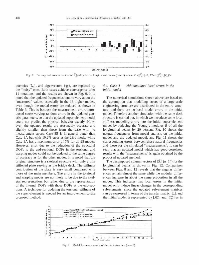
0 ] to [Fse] between two spaces separatelydefined by [Iz] and [Sn]. By comparing the final transfermatrix [Sn] with [ Iz], we can evaluate the correctedmodel errors between the initial model and updatedmodel at sub-element level. As an example on this com-parison, Fig. 8 shows the comparison of the decomposedcolumn vectors of [Sn] (n=11) for the updated longitudi-nal beams with vectors of the unit matrix such as{0, . . , 1, . . ., 0}T12. Thex-axis gives the modal orders ofthe individual longitudinal beam, and they-axis denotesthe modular and angular differences between the vectors[Sn] and the unit vector. It is seen that the initial sub-elements correctly model the rigid-body modes of thelongitudinal beams, since the difference for the first 6

modes are zero; but they predict the strain modes withfault, especially for the higher modes.

4.2. Case 2 — with incomplete measured DOFs

In real life not all the DOFs specified in the analyticalfinite element model could be measured, since someDOFs are physically inaccessible and some are very dif-ficult to measure such as the rotational DOFs. Thereforethe effect of measurement incompleteness on the updat-ing process has to be considered. Two specific cases ofmeasurement incompleteness are investigated. In CaseA, 96 DOFs (only those translational degrees-of-freedomu and v at the master nodes of the end sections) areassumed measured for the first 12 modes. Those unmeas-ured rotational DOFs {φx} r in Eq. (23) are replaced bytheir analytical counterparts in the computation of theeigen-sensitivities. Only the measured DOFs are con-sidered in the updating, and the total number of linearalgebraic equations involved in Eq. (25) is 12×(96+1).In Case B, we select only 60 optimal translational DOFsas “measured” using the Effective Index Method pro-posed by Kammer [26], and expand the “measured”mode shape vectors corresponding to the selected DOFsusing the Kidder (dynamic) expansion method ([27]) tothe full mode shapes in Eq. (23). The use of sensorplacement selection and modal expansion improves thenumerical condition of the updating solution, which isan inverse problem, by improving the condition numberof the sensitivity matrices and increasing the number oflinear algebraic equations to 12×(211+1). Table 3 showsthe updating results of Cases A and B in terms of theerrors in the frequencies after 15 iterations and 11 iter-ations, respectively. It is seen that both cases have sig-nificant improvement in the errors in all the 25 modeswith a maximum error of 12% and 7% for Case A andB, respectively. It is noted that Case B achieves a betterupdating result at fewer iterations than Case A. Case Balso exhibits less error in the updated mode shapes inalmost all 25 modes as shown in Table 2.

4.3. Case 3 — with incomplete measured DOFs andrandom noise

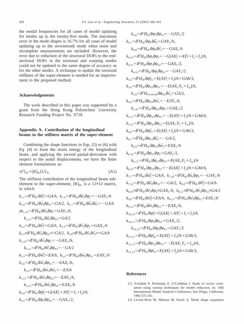
The experimentally identified modal parameters areinevitably contaminated with measurement noise inpractice. We introduce random errors into the “meas-ured” modal data to study the effect of noise on the pro-posed updating process. 1 percent random errors areadded to the first 12 “measured” natural frequencies and5 percent random errors are added to the correspondingincomplete “measured” eigenvectors. Two cases arestudied: Case A is for complete measured DOFs withnoise, and Case B is for incomplete measured DOFs withnoise. The updating processes are similar to Case 1 andCase 2B, respectively, except that the “measured” fre-


Fig. 8. Decomposed column vectors ofSn(n=11) for the longitudinal beams (case 1) whereY1=|{Sn} i|21, Y2=/({ Sn} i,{ I} i)/p.

quencies {λx} r and eigenvectors {φx} r are replaced bythe “noisy” ones. Both cases achieve convergence after11 iterations, and the results are shown in Fig. 9. It isnoted that the updated frequencies tend to vary about the“measured” values, especially in the 13 higher modes,even though the modal errors are reduced as shown inTable 3. This is because the measurement errors intro-duced cause varying random errors in the updated gen-eric parameters, so that the updated super-element modelcould not predict the physical behavior exactly. How-ever, the updated results are reasonably accurate andslightly smaller than those from the case with nomeasurement errors. Case 3B is in general better thanCase 3A but with 10.2% error at the 23rd mode, whileCase 3A has a maximum error of 7% for all 25 modes.However, error due to the reduction of the structuralDOFs to the end-sectional DOFs in the torsional andwarping modes could not be updated to the same degreeof accuracy as for the other modes. It is noted that theoriginal structure is a skeletal structure with only a thinstiffened plate serving as the bridge deck. The stiffnesscontribution of the plate is very small compared withthose of the main members. The errors in the torsionaland warping modes are not likely to be due to the skel-etal representation, but rather due to the representationof the internal DOFs with those DOFs at the end-sec-tions. A technique for updating the torsional stiffness ofthe super-element is needed for an improvement to theproposed method.


4.4. Case 4 — with simulated local errors in theinitial model

The numerical simulations shown above are based onthe assumption that modelling errors of a large-scaleengineering structure are distributed in the entire struc-ture, and there are no local model errors in the initialmodel. Therefore another simulation with the same deckstructure is carried out, in which we introduce some localstiffness modeling errors into the initial super-elementmodel by reducing the Young’s modulusE of all thelongitudinal beams by 20 percent. Fig. 10 shows thenatural frequencies from modal analysis on the initialmodel and the updated model, and Fig. 11 shows thecorresponding errors between these natural frequenciesand those for the simulated “measurements”. It can beseen that an updated model which has good-correlatedresults with the “measurements” is again obtained by theproposed updated method.

The decomposed column vectors of [Sn] (n=14) for thelongitudinal beams is shown in Fig. 12. Comparisonbetween Figs. 8 and 12 reveals that the angular differ-ences remain almost the same while the modular differ-ences increase in about the same proportion in all themodes. This indicates that local errors in the initialmodel only induce linear changes in the correspondingsub-elements, since the updated sub-element matricescan be expressed in terms of the transfer matrix [Sn], andthe initial model is represented by [Mse

0 ] and [Fse0 ] as in



Fig. 11. Errors in the frequency between the initial and updated model (case 4) (T=Torsional modes; W=Warping modes).

Fig. 12. Decomposed column vectors ofSn (n=14) for the longitudinal beams (case 4) whereY1=|{Sn} i|21, Y2=/({ Sn} i,{ I} i)/p.

Eq. (27). We can simulate the occurrence of structuraldamage in the updated sub-element by properly reducingthe physical parameters of the initial model, e.g.E, A,etc., while keeping the transfer matrix [Sn] unchanged.This indicates that the updated super-element models ofintact structures can be updated again into models whichrepresent the damaged structures, by selecting physicalparameters as updating variables. The updated model,therefore, can serve as a basis for further damage identi-fication problems. Detailed studies on this problem willbe separately presented.

It is evident from Table 2 that the updated modelshave mode shapes closer to the “measured” values thanthe initial model, although the errors are still noticeableat higher modes because of the errors due to thereduction of the structural DOFs to the end-sectionalDOFs. Cases with optimal incomplete measurement andmodal expansion give better results than the other cases

with 24.5% and 22.7% at the 18th mode with and with-out noise, respectively. It is again noted that the errorsare larger for the torsional or warping modes.

5. Conclusions

This paper proposes a damage-detection-oriented-model for a large-scale bridge deck. The huge numberof analytical DOFs is significantly reduced and yet themodal sensitivity relationship to small physical changesof the structure is maintained. The initial analyticalmodel is generated using a super-element modelingmethod and the model updating is performed by theintroduction of a new parameterization method into thegenericsub-elements. Numerical case studies have dem-onstrated its effectiveness both within and outside therange of active modes with a maximum of 7% error in


the modal frequencies for all cases of model updatingfor modes up to the twenty-first mode. The maximumerror in the mode shapes is 16.7% for all cases of modelupdating up to the seventeenth mode when noise andincomplete measurements are included. However, theerror due to reduction of the structural DOFs to the end-sectional DOFs in the torsional and warping modescould not be updated to the same degree of accuracy asfor the other modes. A technique to update the torsionalstiffness of the super-element is needed for an improve-ment to the proposed method.

Acknowledgements

The work described in this paper was supported by agrant from the Hong Kong Polytechnic UniversityResearch Funding Project No. S718.

Appendix A. Contribution of the longitudinalbeams to the stiffness matrix of the super-element

Combining the shape functions in Eqs. (5) or (6) withEq. (4) to form the strain energy of the longitudinalbeam, and applying the second partial-derivation withrespect to the nodal displacements, we have the finiteelement formulations as:

{ F} lb5[K]lb{ U} lb (A1)

The stiffness contribution of the longitudinal beam sub-element to the super-element, [K]lb, is a 12×12 matrix,in which

k1,15∂2Hlb/∂u215GA/h, k1,45∂2Hlb/∂u1∂j152GAYC/h

k1,65∂2Hlb/∂u1∂fY15GA/2, k1,75∂2Hlb/∂u1∂u252GA/h

yk1,105∂2Hlb/∂u1∂j25GAYC/h,

k1,125∂2Hlb/∂u1∂fY25GA/2

k2,25∂2Hlb/∂v215GA/h, k2,45∂2Hlb/∂v1∂j15GAXC/h

k2,5=∂2Hlb/∂v1∂fX1=−GA/2, k2,8=∂2Hlb/∂v1∂v2=−GA/h

k2,105∂2Hlb/∂v1∂j252GAXC/h,

k2,115∂2Hlb/∂v1∂fX252GA/2

k3,35∂2Hlb/∂w215EA/h, k3,55∂2Hlb/∂w1∂fX15EAYC/h

k3,65∂2Hlb/∂w1∂fY152EAXC/h,

k3,95∂2Hlb/∂w1∂w252EA/h

k3,115∂2Hlb/∂w1∂fX252EAYC/h,

k3,125∂2Hlb/∂w1∂fY25EAXC/h

k4,45∂2Hlb/∂j215G(AX2

C1AY2C1Ix1Iy)/h,

k4,55∂2Hlb/∂j1∂fX152GAXC/2,

k4,65∂2Hlb/∂j1∂fY152GAYC/2

k4,75∂2Hlb/∂j1∂u25GAYC/h,

k4,85∂2Hlb/∂j1∂v252GAXC/h

k4,105∂2Hlb/∂j1∂j252G(AX2C1AY2

C1Ix1Iy)/h,

k4,115∂2Hlb/∂j1∂fX252GAXC/2,


k5,55∂2Hlb/∂f2X15E(AY2

C1Ix)/h1GAh/3,

k5,65∂2Hlb/∂fX1∂fY152E(AXCYC1Ixy)/h,

k5,85∂2HFUNClb/∂fX1∂v25GA/2,

k5,95∂2Hlb/∂fX1∂w252EAYC/h,

k5,105∂2Hlb/∂fX1∂j25GAXC/2

k5,115∂2Hlb/∂fX1∂fX252E(AY2C1Ix)/h1GAh/6,


k6,65∂2Hlb/∂f2Y15E(AX2

C1Iy)/h1GAh/3,

k6,75∂2Hlb/∂fY1∂u252GA/2,

k6,95∂2Hlb/∂fY1∂w25EAXC/h

k6,105∂2Hlb/∂fY1∂j25GAYC/2,

k6,115∂2Hlb/∂fY1∂fX25E(AXCYC1Ixy)/h

k6,125∂2Hlb/∂fY1∂fY252E(AX2C1Iy)/h1GAh/6,

k7,75∂2Hlb/∂u225GA/h, k7,105∂2Hlb/∂u2∂j252GAYC/h

k7,125∂2Hlb/∂u2∂fY252GA/2, k8,85∂2Hlb/∂v225GA/h

k8,10=∂2Hlb/∂v2∂j2=GAXC/h, k8,11=∂2Hlb/∂v2∂fX2=GA/2

k9,95∂2Hlb/∂w225EA/h, k9,115∂2Hlb/∂w2∂fX25EAYC/h

k9,125∂2Hlb/∂w2∂fY252EAXC/h,

k10,105∂2Hlb/∂j225G(AX2

C1AY2C1Ix1Iy)/h,

k10,115∂2Hlb/∂j2∂fX25GAXC/2,


k11,115∂2Hlb/∂f2X25E(AY2

C1Ix)/h1GAh/3,


k12,125∂2Hlb/∂f2Y25E(AX2

C1Iy)/h1GAh/3,

References

[1] Avitabile P, Pechinsky F, O’Callahan J. Study of vector corre-lation using various techniques for model reduction. In: 10thInternational Modal Analysis Conference, San Diego, California,1992:572–83.

[2] Levine-West M, Milman M, Kissil A. Mode shape expansion


techniques for prediction: experimental evaluation. AIAA Journal1996;34(4):821–9.

[3] Stubbs N, Broome TH, Osegueda R. Nondestructive constructionerror detection in large space structures. AIAA Journal1990;28:146–52.

[4] Kondo I, Hamamoto T. Local damage detection of flexible off-shore platforms using ambient vibration measurement. In: Pro-ceedings of the 4th International Offshore and Polar EngineeringConference, Osaka, Japan, 1994;4:400–7

[5] Wang WL, Du ZR. Structure vibration and dynamic substructuremethods. Shanghai: Fudan University Press, 1985.

[6] Lu X. Simplified dynamic condensation in multi-substructure sys-tems. Comput Struct 1988;30:851–4.

[7] Kim HM, Bartkowicz TJ. A two-step structural damage detectionapproach with limited instrumentation. J of Vibration and Acous-tics, ASME 1997;119(2):258–64.

[8] Lantau fixed crossing: wind and structural health monitoring mas-terplan — Assessment strategy of possible structural damage inthe Tsing Ma Bridge, Kap Shui Bridge, and Ting Kau Bridge.Department of Civil and Structural Engineering, Hong KongPolytechnic University, Hung Hom, Kowloon, Hong Kong, 1998.

[9] Mottershead JE, Friswell MI. Model updating in structuraldynamics: a survey. Journal of Sound and Vibration1993;167(2):347–75.

[10] Berman A. Mass matrix correction using an incomplete set ofmeasured models. AIAA Journal 1979;17(10):1147–8.

[11] Berman A, Nagy EJ. Improvement of large analytical modelusing modal test data. AIAA Journal 1983;21(8):1168–73.

[12] Brauch A. Methods of reference basis for identification of lineardynamic structures. AIAA Journal 1984;22(4):561–3.

[13] Kabe AM. Stiffness matrix adjustment using modal data. AIAAJournal 1985;23(9):1431–6.

[14] Caesar B, Peter J. Direct updating of dynamic mathematical mod-els from modal testing data. AIAA Journal 1987;25(11):1494–9.

[15] Collins JD, Hart GC, Hasselman TK, Kennedy B. Statisticalidentification of structures. AIAA Journal 1974;12(1):185–90.

[16] Lin RM, Lim MK, Du H. Improved inverse eigensensitivitymethod for structural analytical model updating. ASME Journalof Vibration and Acoustics 1995;117:192–8.

[17] Chen JC, Graba JA. Analytical model improvement using modaltesting results. AIAA Journal 1980;12(2):684–90.

[18] Hoff C, Natke HG. Correction of a finite element model by input–output measurements with application to a radar tower. The Inter-national Journal of Analytical and Experimental Modal Analysis1989;4(1):1–7.

[19] Gladwell GML, Ahmadian H. Generic element matrices suitablefor finite element model updating. Mechanical Systems and Sig-nal Processing 1995;9(6):601–14.

[20] Ahmadian H, Gladwell GML, Ismail F. Parameter selection stra-tegies in finite element model updating. Journal of Vibration andAcoustics, ASME 1997;119:37–45.

[21] Natke HG. Updating computational models in the frequencydomain based on measured data: a survey. Probabilistic Engineer-ing Mechanics 1988;3(1):28–35.

[22] Ross RG. Synthesis of stiffness and mass matrices from experi-mental vibration modes. In: National Aeronautics and SpaceEngineering and Manufacturing Meeting, Society of AutomotiveEngineers, Los Angeles, California, 1971:2627–35.

[23] SAP2000 Analysis Reference (Volume I), Version 6.1. Com-puters and Structures, Inc., Berkeley, California, 1997.

[24] Keye S. Prediction of modal and frequency response data froma validated finite element model. In: Proceedings of the SecondInternational Conference on Identification of Engineering Sys-tems, 1997:122–34.

[25] Friswell MI, Mottershead JE. Finite element model updating instructural dynamics. Kluwer Academic, 1995.

[26] Kammer DC. Sensor placement for on-orbit modal identificationand correlation of large space structures. Journal of Guidance andControl 1991;14(2):251–9.

[27] Kidder RL. Reduction of structural frequency equations. AIAAJournal 1973;11(6):892.

efficient numerical model for the damage detection of large scale structure

Documents