efficient optimization of all-terminal...

EFFICIENT OPTIMIZATION OF ALL-TERMINAL RELIABLE NETWORKS USINGAN EVOLUTIONARY APPROACH

Berna Dengiz and Fulya AltiparmakDepartment of Industrial Engineering

Gazi University06570 Maltepe, Ankara Turkey

e-mail: [email protected]

Alice E. Smith, Senior Member IEEEDepartment of Industrial Engineering

University of PittsburghPittsburgh, PA 15261

email: [email protected]

IEEE Transactions on ReliabilityTo Appear March 1997

1

Efficient Optimization Of All-Terminal Reliable Networks Using AnEvolutionary Approach

Berna DengizGazi University, Ankara Turkey

Fulya AltiparmakGazi University, Ankara Turkey

Alice E. Smith, Senior Member IEEE1

University of Pittsburgh

Key Words - network reliability, heuristic optimization, genetic algorithms, combinatorial

optimization, communication network, Monte Carlo simulation

Summary & Conclusions - The use of computer communication networks has been rapidly

increasing to 1) share expensive hardware and software resources, and 2) provide access to main

systems from distant locations. The reliability and the cost of these systems are important

considerations that are largely determined by network topology. Network topology consists of

nodes and the links between nodes. The selection of optimal network topology is an NP-hard

combinatorial problem so that the classical enumeration based methods grow exponentially with

network size. In this study, a heuristic search algorithm inspired by evolutionary methods is

presented to solve the all-terminal network design problem when considering cost and reliability.

The genetic algorithm heuristic is considerably enhanced over conventional implementations to

improve effectiveness and efficiency. This general optimization approach is shown to be

computationally efficient and highly effective on a large suite of test problems with search spaces

up to 2 × 1090.

1 Corresponding author.

2

1. INTRODUCTION

Acronyms

GA genetic algorithm

GAKBS GA with knowledge-based steps

SGA simple GA

An important stage of the design of communication networks is to find the best layout of

components to minimize cost while meeting a performance criterion, such as transmission delay,

throughput or reliability [1]. This paper focuses on large scale backbone communication network

[2] design where the relevant reliability metric is all-terminal network reliability (also called

overall network reliability); defined as the probability that every pair of nodes can communicate

with each other [1, 3]. The problem of optimal design of link topology can be formulated as a

combinatorial problem where the selection of components either maximizes reliability, or

minimizes cost. This problem is NP-hard [4], and further compounding this is the computational

effort required to calculate or estimate network reliability.

This problem has been studied with both enumerative based methods and heuristic methods.

Jan et al. [1] developed an algorithm using decomposition based on branch-and-bound to

minimize link costs with a minimum network reliability constraint; this is computationally tractable

for fully connected networks up to 12 nodes. Chopra et al. [6] and Aggarwal et al. [5] both used

greedy heuristic approaches. Venetsanopoulos and Singh [7] used a two step heuristic for

minimizing cost subject to a reliability constraint. GA has recently been used in combinatorial

optimization approaches to reliable design, mainly for series-parallel systems [8-10]. For network

design, Kumar et al. [11, 12] developed a GA considering diameter, distance and reliability to

design and expand computer networks. Deeter and Smith present a GA for a generalized network

design problem with alternative link reliabilities [13]. This paper also uses a GA, but significantly

customizes it to the all-terminal design problem to result in an effective and efficient optimization

methodology. Furthermore, this approach is demonstrated on a large test suite of problems,

3

including networks with up to 300 possible links. Previous papers have demonstrated their

optimization procedures on small networks (usually less than 10 nodes), thus the important issue

of scale-up is left unanswered.

A significant issue is the calculation of the reliability of candidate network topologies. When

minimizing cost subject to a minimum reliability constraint, the network reliability calculation is

necessary to determine feasibility of the candidate design. When maximizing reliability subject to

a maximum cost constraint, the network reliability calculation is the objective function. It either

case, this calculation is a critical part of evaluating each candidate network topology, however it

is also problematic since it involves considerable computational effort. All known analytic

methods for all-terminal network reliability calculation have worst case computation times which

grow exponentially in the size of the network considered. Monte Carlo simulation methods, for

which computation time grows only slightly faster than linear with network size, are suitable for

large networks [14]. An efficient Monte Carlo simulation technique [15] is used to estimate all-

terminal reliability in this paper. To further reduce the computational effort required, candidate

networks must meet a 2-connectivity measure [16], after verifying that a spanning tree exists

using the method of [17]. Then an upper bound on reliability by [18] is used to screen candidate

networks prior to the estimation of reliability using simulation. However, any method of

calculating or estimating network reliability could be incorporated into the evolutionary

optimization methodology presented in this paper.

Section 2 gives the mathematical formulation of the optimization problem and its

assumptions. Section 3 gives the algorithm used in this paper. Section 4 provides the results and

discussion of applying the optimization methodology to a suite of test problems.

Notation

G a probabilistic graph

N set of nodes (terminals)

L set of links (edges, arcs)

4

(i,j) a link between nodes i and j

p,q link reliability, link unreliability for all links; p+q = 1

xij decision variable, xij ∈{0,1}

x a link topology of {x11,x12, ... , xij, ... , xN,N-1}

R(x) all-terminal reliability of x

Ro network reliability requirement

Z objective function

cij cost of (i,j)

cMAX the maximum value of cij

δ 0, if Rel(x) ≥ Ro; 1, if Rel(x) < Ro

gMAX maximum number of generations in genetic algorithm

n population size of genetic algorithm

rc crossover rate of genetic algorithm

rm mutation rate of genetic algorithm

2. STATEMENT OF THE PROBLEM

A communication network can be modeled by a probabilistic graph G = (N, L, p), in which N

and L correspond to computer sites and communication links, respectively. Any graph G = (N, L)

is connected if there is at least one path between every pair of nodes N ,N i j ∈ N edges, which

minimally requires a spanning tree with N-1 edges.

Assumptions

1. The location of each network node is given.

2. Nodes are perfectly reliable.

3. Each cij and p are fixed and known.

4. Each link is bi-directional.

5. There are no redundant links in the network.

5

6. Links are either operational or failed.

7. The failure of links are s-independent.

8. No repair is considered.

The optimization problem is:

Minimize Z =i

N

j i

N

=

−

= +∑ ∑

1

1

1

cij xij (1)

Subject to : R(x) ≥ Ro

where { }x 0,1ij ∈ is the decision variable and R(x) is the system reliability.

At any instant of time, only some edges of G may be operational. A state of G is a sub-graph

(N,L′) with L′∈L, where L′ is the set of operational edges. An operational state is generally

called a pathset, and a minimal operational state is termed a min-path. A failed state L′ is called L

\ L′ (a cutset) and when L′ is a maximal failed state L \ L′ is a mincut [19]. The network

reliability of state L′ ⊆ L is shown below : p q

(L \ L Lall operational states

''l l

ll ∈∈∏∏∑

)

(2)

Summing this state occurrence probability over all operational states gives the network system

reliability. However, the exponential number of states makes such a computation infeasible, even

for networks of moderate sizes [19]. All current exact algorithms of reliability computation for

general networks are based on the enumeration of states, minpaths or mincuts [20-24]. But few

of them give a little practical improvement over complete state enumeration, while others still

examine exponentially many states, minpaths or mincuts [19]. Therefore, estimation of network

reliability is commonly used for non-trivial sized networks, and this paper uses an efficient Monte

Carlo based simulation as described in section 3.

3. SOLUTION ALGORITHM

A GA was selected as the heuristic optimization vehicle because of its flexibility and

robustness as demonstrated on many NP-hard problems, including those of reliability design [8-

6

13]. GA is a meta-heuristic inspired by the biological paradigm of evolution. They were

pioneered by Holland [25], De Jong [26], and Goldberg [27] in the context of continuous non-

linear optimization, and later extended by various authors [e.g., 28-30] to combinatorial problems.

In GA, the search space is composed of candidate solutions to the problem, each represented by a

string, termed a chromosome. Each chromosome has an objective function value, called the

fitness. A set of chromosomes together with their associated fitness is called the population. This

population, at a given iteration of the GA, is referred to as a generation.

There are three main steps in the repeat loop for GA:

1) The process of selecting strings from the current generation to be parents of the next

generation with preference for fitter strings. This is the selection process for

reproduction.

2) The process of combining two selected strings to generate new children strings, which

is called crossover. Probabilistically, components of a chromosome are perturbed

while generating a child. This process is called mutation. Together, crossover and

mutation comprise reproduction.

3) Computation of the fitness value using the objective function of each new solution.

The steps in the GA approach in this research are discussed below, followed by a flowchart of the

algorithm.

3.1. Coding Structure

Each x represents a candidate network design with the size of the string equal to N(N-1)/2,

the number of possible links in a fully connected network.2 For example, Figure 1 shows a simple

network whose base graph consists of 5 nodes and 10 possible links, but with only 7 links present.

Figure 1 here.

The string representation of this network is:

2 This is reduced for networks where not all possible links are permitted, as demonstrated on test problems 18 - 20.

7

[ ][ ] 1 1 0 1 1 0 1 1 0 1

x x x x x x x x x x 12 13 14 15 23 24 25 34 35 45

3.2. Initial Population

The initial population in GA can be obtained randomly or by using a heuristic method

(“seeding” the population). In this paper, the initial population consists of a set of connected

networks which are also 2-connected but is otherwise generated in a random fashion with

preference to combinations yielding high reliability. The 2-connectivity measure is used as a

preliminary screening, since it is usually a property of highly reliable networks. The selection of

the probability values which are used in deciding whether a link exists or not is an important stage

for the efficient generation of such an initial population. Table 1 shows the probability intervals

used in this research, established by exploratory research.

Insert Table 1 Here

3.3. Genetic Algorithm Parameters

The choice of parameters for GA can affect performance of the algorithm. These parameters

include n, rc and rm. There have been many different studies to find the optimal control

parameters for GA, however this is little in the way of useful guidance. Instead, a set of

experiments are usually run to establish parameter values which work well and to gauge the

sensitivity of the GA to alterations in those values. For this study, the best results were: n = 20,

rc = 0.95, and rm = 0.05.

3.4. Selection Mechanism, Genetic Operators, Replacement Strategy

The approach in this paper uses the conventional GA operators of roulette wheel selection,

single point crossover and bit flip mutation. See Goldberg [27] for a definition of these. Below is

an example of the single point crossover strategy with the splice point after x15. and bit flip

mutation used in this research:

Parent 1

[ ][ ] 1 1 0 1 1 0 1 1 0 1

x x x x x x x x x x 12 13 14 15 23 24 25 34 35 45

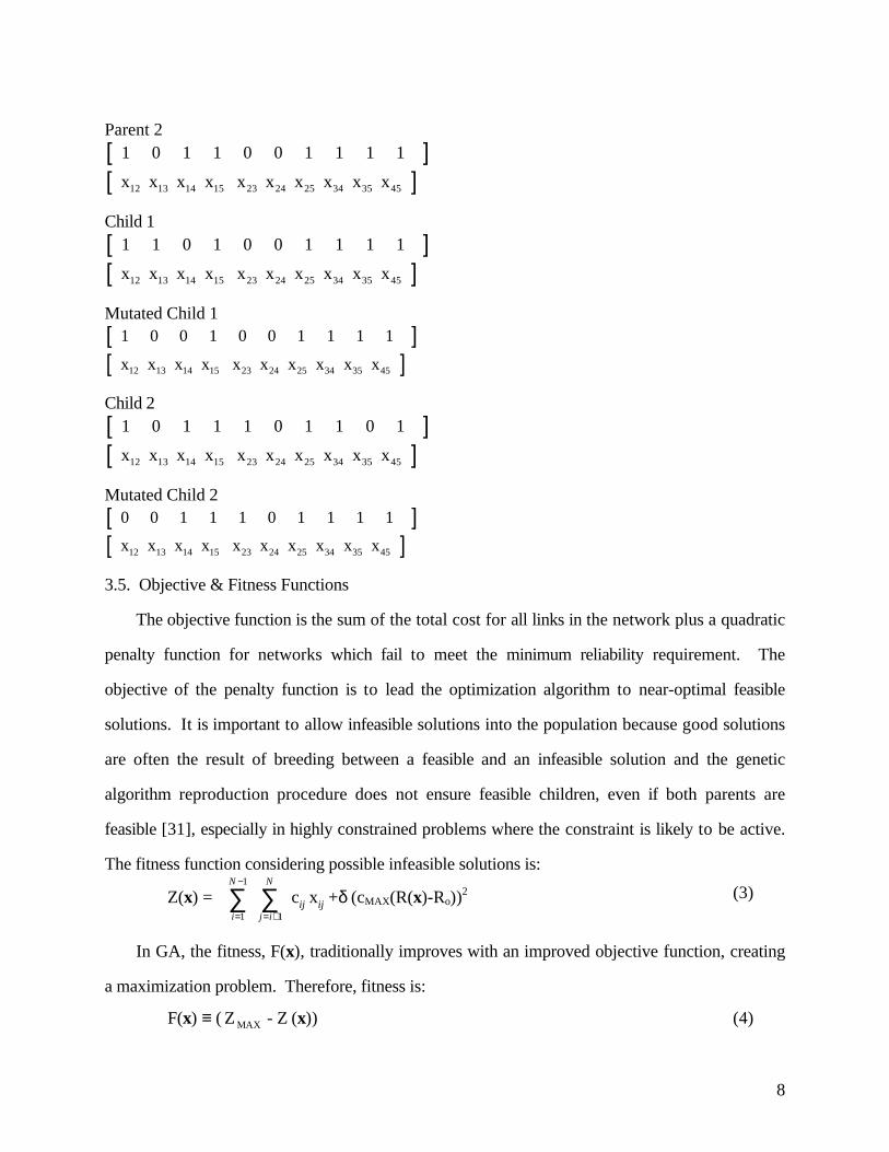
8

Parent 2

[ ][ ] 1 0 1 1 0 0 1 1 1 1

x x x x x x x x x x 12 13 14 15 23 24 25 34 35 45

Child 1

[ ][ ] 1 1 0 1 0 0 1 1 1 1

x x x x x x x x x x 12 13 14 15 23 24 25 34 35 45

Mutated Child 1[ ][ ] 1 0 0 1 0 0 1 1 1 1

x x x x x x x x x x 12 13 14 15 23 24 25 34 35 45

Child 2

[ ][ ] 1 0 1 1 1 0 1 1 0 1

x x x x x x x x x x 12 13 14 15 23 24 25 34 35 45

Mutated Child 2[ ][ ] 0 0 1 1 1 0 1 1 1 1

x x x x x x x x x x 12 13 14 15 23 24 25 34 35 45

3.5. Objective & Fitness Functions

The objective function is the sum of the total cost for all links in the network plus a quadratic

penalty function for networks which fail to meet the minimum reliability requirement. The

objective of the penalty function is to lead the optimization algorithm to near-optimal feasible

solutions. It is important to allow infeasible solutions into the population because good solutions

are often the result of breeding between a feasible and an infeasible solution and the genetic

algorithm reproduction procedure does not ensure feasible children, even if both parents are

feasible [31], especially in highly constrained problems where the constraint is likely to be active.

The fitness function considering possible infeasible solutions is:

Z(x) =i

N

j i

N

=

−

= +∑ ∑

1

1

1

cij xij +δ (cMAX(R(x)-Ro))2 (3)

In GA, the fitness, F(x), traditionally improves with an improved objective function, creating

a maximization problem. Therefore, fitness is:

F(x) ≡ ( Z - ZMAX (x)) (4)

9

where ZMAX is the largest (worst) value of (3) for the current population.

3.6. Network Reliability

The GA methodology in this paper uses three reliability estimations to tradeoff accuracy with

computational effort. An ideal strategy employs only the computationally intensive method of

Monte Carlo simulation (or exact network reliability calculation) on the optimal network design.

Since GA is an iterative algorithm, this ideal cannot be attained because many candidate networks

must be evaluated during the search. Therefore, screening of candidate network designs is done:

• A connectivity check for a spanning tree is made on all new network designs using the

method of [17].

• For networks which pass this check, the 2-connectivity measure [16] is made by

counting the node degrees.

• For networks which pass both of these preliminary checks, Jan’s upper bound [18] is

used to compute the upper bound of reliability of a candidate network, RU(x).

This upper bound in used in the calculation of the objective function (3) for all networks except

those which are the best found so far (xBEST). Networks which have RU(x) ≥ Ro and the lowest

cost so far are sent to the Monte Carlo subroutine for more precise estimation of network

reliability using an efficient Monte Carlo technique by Yeh et al. [15]. The simulation is done for

3000 iterations for each candidate network for all problems studied in this paper.

3.7. Termination Condition

The criterion is gMAX, which varies according to the size of the network, N, under study.

Algorithm

Step 1: Generate the initial population, k = 1 to n, randomly according to the link

probabilities in Table 1, discarding any solutions which fail to meet the 2-connectivity

requirement. Calculate the fitness of each candidate network in the population using (3)

and (4) and Jan’s upper bound as R(x), except for the lowest cost network with RU(x) ≥ Ro.

For this network, xBEST, use the Monte Carlo estimation of R(x) in (4). g = 1.

Step 2: Select two candidate networks from current population by the selection mechanism.

10

Step 3: To obtain two children candidate networks, apply reproduction to the selected

networks using rc and rm.

Step 4: Determine the 2-connectivity of each new child. Discard any that do not satisfy 2-

connectivity.

Step 5: Calculate RU(x) for each child and compute its objective function using (3).

Step 6: If the number of new children < n-1 go to Step 2.

Step 7: Replace parents with children, retaining xBEST from the previous generation.

Step 8: Sort the new generation in increasing order of Z with k the indices of a candidate

network. k = 1 to n.

a) If Z(xk) < Z(xBEST), then estimate the system reliability of this network using Monte

Carlo simulation, else go to Step 9.

b) xBEST = xk. Go to Step 9.

Step 9 : Calculate the fitness value, F(x), using (4) for each network in the new population.

Step 10 : If g = gMAX stop, else go to Step 2 and g = g+1.

4. RESULTS & DISCUSSION

4.1 Results

Several comparisons are used to judge the effectiveness and efficiency of the GA described in

section 3, which will be termed GAKBS. The first comparison is against a GA which does not

include the problem specific structure, termed SGA. In SGA, the initial population consists of

connected networks, generated using a constant probability value of 0.5 to generate a link. These

networks are not subject to the 2-connectivity screening calculation. System reliability is then

estimated on all networks using the improved Monte Carlo procedure. The second comparison is

against the branch-and-bound method of Jan et al. [1].

The test problems are summarized in Table 2 and detailed in the Appendix. These problems

are both fully connected and non-fully connected networks (viz., only a subset of L is possible for

11

selection). N of the connected networks ranges from 5 to 25. The available links of the non-fully

connected networks were randomly generated and were 1.5 times N. The link costs for all

networks were randomly generated over [1,100] except for problems 3 through 5 which used

costs over [1,150]. Each problem for the GA was run 10 times, each time with a different random

number seed. Optimal solutions, as obtained by the method of Jan et al. [1], are also given in

Table 2 with topologies shown in the Appendix. Jan’s method cannot be practically used on the

larger problems (numbers 15-17) because of the computational effort of the branch-and-bound

procedure. As shown, GAKBS gives the optimal value for the all replications of problems 1 - 3

and finds optimal for all but two of the problems for at least one run of the 10. The two with

suboptimal results (12 and 13) are very close to optimal.

Insert Table 2 Here

The performance of SGA and GAKBS were compared for all networks with the enhanced

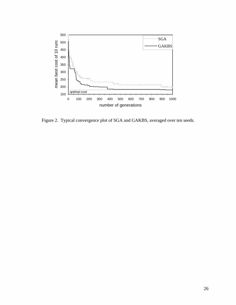
GA converging significantly faster to a value closer to optimum. Figure 2 is a typical

convergence plot showing the best cost network for a single problem averaged over ten runs with

different seeds. Speed of convergence is important because the reliability calculation, especially

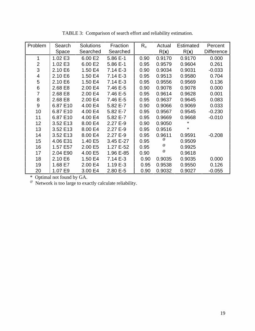
for larger problems, precludes extensive search of the problem space. Table 3 lists the search

space for each problem along with the proportion actually searched by the GAKBS during a

single run (n × gMAX). gMAX ranged from 30 to 20000, depending on problem size. This

proportion is an upper bound because GA’s can (and often do) revisit solutions already

considered earlier in the evolutionary search. It can be seen that the GA approach examines only

a very tiny fraction of the possible solutions for the larger problems, yet still yields optimal or

near-optimal solutions. Table 3 also compares the efficacy of the Monte Carlo estimation of

network reliability. The exact network reliability is calculated using a backtracking algorithm also

used by Jan et al. [1] and compared to the estimated counterpart for the final network for those

problems where the GA found optimal. The reliability estimation of the Monte Carlo method is

unbiased and is always within 1% of the exact network reliability. Since the computation time for

the Monte Carlo method is constant with network size, and estimation accuracy does not degrade

12

with an increase in L, this simulation estimation is a very effective surrogate for an exact network

reliability calculation.

Figure 2 here.

Insert Table 3 Here

4.2 Discussion

In this study, a stochastic search algorithm inspired by evolution was developed to solve

network topology design with minimum cost subject to a reliability constraint. The strengths of

this evolutionary approach are almost non-increasing computational effort, effective optimization

and flexibility. Since GA is an iterative algorithm and improvement is typically diminishing (as in

Figure 2), it may be terminated at any time and still return good results. The computational effort

over the test problems studied did not vary significantly although network size increased by many

orders of magnitude. The GA returned optimal or near-optimal solutions on every run regardless

of problem instance, problem size or random number seed. The methodology is very flexible and

alternative objectives (e.g., maximize reliability subject to a cost constraint) and alternative

methods of reliability calculation (e.g., backtracking or another Monte Carlo method) could be

easily substituted for those used in this research.

ACKNOWLEDGMENT

Part of this study was funded by The Scientific and Technical Research Council of Turkey

(STRCT). A. E. Smith is pleased to acknowledge the support of the U.S. National Science

Foundation CAREER grant DMI 95-02134.

REFERENCES

[1] R.-H. Jan, F.-J. Hwang, S.-T. Chen, “Topological optimization of a communicationnetwork subject to a reliability constraint,” IEEE Transactions on Reliability, vol 42, 1993 Mar,pp 63-70.

13

[2] R. R. Boorstyn, H. Frank, “Large scale network topological optimization,” IEEETransactions on Communications, vol Com-25 1977 Jan, pp 29-37.

[3] C. J. Colbourn, The Combinatorics of Network Reliability, Oxford University Press 1987.

[4] M. R. Garey, D. S. Johnson, Computers and Intractability: A Guide to the Theory of NP-Completeness, 1979; W. H. Freeman and Co.

[5] K. K. Aggarwal, Y. C. Chopra, J. S. Bajwa, “Topological layout of links for optimising theoverall reliability in a computer communication system,” Microelectronics and Reliability, vol 22,1982, pp 347-351.

[6] Y. C. Chopra, B. S. Sohi, R. K. Tiwari, K. K. Aggarwal, “Network topology formaximizing the terminal reliability in a computer communication network,” Microelectonics &Reliabiliy, vol 24, 1984, pp 911-913.

[7] A. N. Venetsanopoulos, I. Singh, “Topological optimization of communication networkssubject to reliability constraints,” Problem of Control and Information Theory, vol 15, 1986, pp63-78.

[8] D. W. Coit, A. E. Smith, “Reliability optimization of series-parallel systems using agenetic algorithm,” IEEE Transactions on Reliability, vol 45, 1996 Jun, pp 254-260.

[9] K. Ida, M. Gen, T. Yokota, “System reliability optimization with several failure modes bygenetic algorithm,” Proceedings of 16th International Conference on Computers and IndustrialEngineering, 1994, pp 349-352.

[10] L. Painton, J. Campbell, “Genetic algorithms in optimization of system reliability,” IEEETransactions on Reliability, vol 44, 1995 Jun, pp 172-178.

[11] A. Kumar, R. M. Pathak, Y. P. Gupta, H. R. Parsaei, “A genetic algorithm for distributedsystem topology design,” Computers and Industrial Engineering, vol 28, 1995, pp 659-670.

[12] A. Kumar, R. M. Pathak, Y. P. Gupta, “Genetic-algorithm-based reliability optimization forcomputer network expansion,” IEEE Transactions on Reliability, vol 44, 1995 Mar, pp 63-72.

[13] D. L. Deeter, A. E. Smith, “Heuristic optimization of network design considering all-terminal reliability,” Proceedings of the Reliability and Maintainability Symposium 1997, toappear.

[14] M. Ball, R. M. Van Slyke, “Backtracking algorithms for network reliability analysis,”Annals of Discrete Mathematics, vol 1, 1977, pp 49-64.

[15] M.-S. Yeh, J.-S. Lin, W.-C. Yeh, “A new Monte Carlo method for estimating networkreliability,” Proceedings of the 16th International Conference on Computers & IndustrialEngineering, 1994, pp 723-726.

[16] L. G. Roberts, B. D. Wessler, “Computer network development to achieve resourcesharing,” Proceedings of the Spring Joint Computer Conference of AFIPS, 1970, pp 543-549.

[17] J. E. Hopcroft, J. D. Ullman, “Set merging algorithms,” SIAM Journal of Computers, vol 2,1973 Jun, pp 296-303.

[18] R.-H. Jan, “Design of reliable networks,” Computers and Operations Research, vol 20,1993, pp 25-34.

14

[19] C. J. Colbourn, “Combinatorial aspects of network reliability,” Annals of OperationsResearch, vol 33, 1991, pp 3-15.

[20] K. K. Aggarwal, S. Rai, “Reliability evaluation in computer-communication networks,”IEEE Transactions on Reliability, vol R-30, 1981 Apr, pp 32-35.

[21] K. K. Aggarwal, Y. C. Chopra, J. S. Bajwa, “Reliability evaluation by networkdecomposition,” IEEE Transactions on Reliability, vol R-31, 1982 Oct, pp 355-358.

[22] H. Nakawaza, “Decomposition method for computing the reliability of complex networks,”IEEE Transactions on Reliability, vol R-30, 1981 Aug, pp 289-292.

[23] S. Rai, “A cutset approach to reliability evaluation in communication networks,” IEEETransactions on Reliability, vol R-31, 1982 Dec, pp 428-431.

[24] J. K. Cavers, “Cutset manipulations for communication network reliability estimation,”IEEE Transactions on Communications, vol Com-23, 1975 Jun, pp 569-575.

[25] J. H. Holland, Adaptation in Natural and Artificial Systems, 1975; University of MichiganPress.

[26] K. A. DeJong, An Analysis of the Behavior of a Class of Genetic Adaptive Systems, Ph.D.Thesis, University of Michigan 1975.

[27] D. E. Goldberg, Genetic Algorithms in Search, Optimization, and Machine Learning,1989; Addison-Wesley.

[28] J. P. Cohoon, S. U. Hedge, W. N. Martin, D. S. Richards, “Distributed genetic algorithmsfor the floorplan design problem,” IEEE Transactions on Computer Aided Design of IntegratedCircuits and Systems, vol 10, 1991 Apr, pp 483-492.

[29] J. E. Biegel, J. J. Davern, “Genetic algorithms and job shop scheduling,” Computers andIndustrial Engineering, vol 19, 1990, pp 81-91.

[30] H. Muhlenbein, M. G. Schleuter, O. Kramer, “Evolution algorithms in combinatorialoptimization,” Parallel Computing vol 7, 1988 Apr, pp 65-85.

[31] D. W. Coit, A. E. Smith, D. M. Tate, “Adaptive penalty methods for genetic optimizationof constrained combinatorial problems,” INFORMS Journal on Computing, vol 8, 1996 Spr, pp173-182.

AUTHORS

Dr. Berna Dengiz; Department of Industrial Engineering; Gazi University; 06570 Maltepe, Ankara

Turkey

Internet (e-mail): [email protected]

15

Berna Dengiz is an Associate Professor of Industrial Engineering and also Vice Dean of the

Faculty of Engineering. Her field of study is the modeling and optimization of complex systems.

Her research has been sponsored by TUBITAK - The Scientific and Technical Research Council

of Turkey. Dr. Dengiz is a member of SCS - Society for Computer Simulations, Operations

Research Society of Turkey, Informatics Society of Turkey and Statistics Society of Turkey.

Dr. Fulya Altiparmak; Department of Industrial Engineering; Gazi University; 06570 Maltepe,

Ankara Turkey

Fulya Altiparmak is a Research Assistant of Industrial Engineering. She received a B.Sc.

(1987), M.Sc. (1990) and Ph.D. (1996) in Industrial Engineering from Gazi University. Her

research concerns reliability optimization and modeling of complex systems using stochastic

optimization techniques. She is a member of the Operations Research Society of Turkey.

Dr. Alice E. Smith; Department of Industrial Engineering; University of Pittsburgh; Pittsburgh,

PA 15261 USA.

Internet (e-mail): [email protected]

Alice E. Smith is Associate Professor of Industrial Engineering and Board of Visitors

Faculty Fellow at the University of Pittsburgh. Her research in modeling and optimization of

complex systems has been funded by Lockheed Martin Corporation, ABB Daimler Benz

Transportation (ADtranz), the National Institute of Standards (NIST), the Ben Franklin

Technology Center of Western Pennsylvania and the National Science Foundation (NSF), from

which she was awarded a CAREER grant in 1995. She is a member of the Design and

Manufacturing Editorial Board of IIE Transactions and is an associate editor of INFORMS

Journal on Computing, International Journal of Smart Engineering System Design, and

16

Engineering Design and Automation. She is a Senior Member of IIE, IEEE and SWE, a member

of INFORMS and ASEE, and a Registered Professional Engineer in the Commonwealth of

Pennsylvania.

17

TABLE 1: Probability values used to generate the initial population.

Number of Nodes (N) Probability Values10 (0.15-0.60)20 (0.15-0.50)30 (0.10-0.30)

18

TABLE 2: Comparison of results.

Results of Genetic Algorithms@

Problem N L p Ro OptimumCost*

BestCost

MeanCost

Coef. ofVariation

FULLY CONNECTED NETWORKS 1 5 10 0.80 0.90 255 255 255.0 0 2 5 10 0.90 0.95 201 201 201.0 0 3 7 21 0.90 0.90 720 720 720.0 0 4 7 21 0.90 0.95 845 845 857.0 0.0185 5 7 21 0.95 0.95 630 630 656.0 0.0344 6 8 28 0.90 0.90 203 203 205.4 0.0198 7 8 28 0.90 0.95 247 247 249.5 0.0183 8 8 28 0.95 0.95 179 179 180.3 0.0228 9 9 36 0.90 0.90 239 239 245.1 0.0497

10 9 36 0.90 0.95 286 286 298.2 0.0340 11 9 36 0.95 0.95 209 209 227.2 0.0839 12 10 45 0.90 0.90 154 156 169.8 0.0618 13 10 45 0.90 0.95 197 205 206.6 0.0095 14 10 45 0.95 0.95 136 136 150.4 0.0802 15 15 105 0.90 0.95 --- 317 344.6 0.0703 16 20 190 0.95 0.95 --- 926 956.0 0.0304 17 25 300 0.95 0.90 --- 1606 1651.3 0.0243

NON FULLY CONNECTED NETWORKS 18 14 21 0.90 0.90 1063 1063 1076.1 0.0129 19 16 24 0.90 0.95 1022 1022 1032.0 0.0204 20 20 30 0.95 0.90 596 596 598.6 0.0052

* Found by the method of Jan et al. [1].@ Over ten runs.

19

TABLE 3: Comparison of search effort and reliability estimation.

Problem SearchSpace

SolutionsSearched

FractionSearched

Ro ActualR(x)

EstimatedR(x)

PercentDifference

1 1.02 E3 6.00 E2 5.86 E-1 0.90 0.9170 0.9170 0.000 2 1.02 E3 6.00 E2 5.86 E-1 0.95 0.9579 0.9604 0.261 3 2.10 E6 1.50 E4 7.14 E-3 0.90 0.9034 0.9031 -0.033 4 2.10 E6 1.50 E4 7.14 E-3 0.95 0.9513 0.9580 0.704 5 2.10 E6 1.50 E4 7.14 E-3 0.95 0.9556 0.9569 0.136 6 2.68 E8 2.00 E4 7.46 E-5 0.90 0.9078 0.9078 0.000 7 2.68 E8 2.00 E4 7.46 E-5 0.95 0.9614 0.9628 0.001 8 2.68 E8 2.00 E4 7.46 E-5 0.95 0.9637 0.9645 0.083 9 6.87 E10 4.00 E4 5.82 E-7 0.90 0.9066 0.9069 0.033

10 6.87 E10 4.00 E4 5.82 E-7 0.95 0.9567 0.9545 -0.230 11 6.87 E10 4.00 E4 5.82 E-7 0.95 0.9669 0.9668 -0.010 12 3.52 E13 8.00 E4 2.27 E-9 0.90 0.9050 * 13 3.52 E13 8.00 E4 2.27 E-9 0.95 0.9516 * 14 3.52 E13 8.00 E4 2.27 E-9 0.95 0.9611 0.9591 -0.208 15 4.06 E31 1.40 E5 3.45 E-27 0.95 @ 0.9509 16 1.57 E57 2.00 E5 1.27 E-52 0.95 @ 0.9925 17 2.04 E90 4.00 E5 1.96 E-85 0.90 @ 0.9618 18 2.10 E6 1.50 E4 7.14 E-3 0.90 0.9035 0.9035 0.000 19 1.68 E7 2.00 E4 1.19 E-3 0.95 0.9538 0.9550 0.126 20 1.07 E9 3.00 E4 2.80 E-5 0.90 0.9032 0.9027 -0.055

* Optimal not found by GA.@ Network is too large to exactly calculate reliability.

20

APPENDIX

COST MATRICES OF FULLY CONNECTED NETWORKS

Problems 1 and 2: 5 nodes, 10 arcs

1 2 3 4 51 - 32 54 62 252 - 34 58 453 - 36 524 - 295 -

Problem 1 Optimum : {1,2}{1,3}{1,5}{2,3}{2,5}{3,4}{4,5}Problem 2 Optimum : {1,2}{1,5}{2,3}{2,5}{3,4}{4,5}

Problems 3, 4 and 5: 7 nodes, 21 arcs

1 2 3 4 5 6 71 - 125 150 125 150 150 1302 - 75 100 150 200 2503 - 75 90 250 2004 - 75 100 1505 - 75 1006 - 757 -

Problem 3 Optimum : {1,2}{1,7}{2,3}{2,4}{3,5}{4,5}{5,6}{6,7}Problem 4 Optimum : {1,2}{1,7}{2,3}{2,4}{3,5}{4,5}{5,6}{5,7}{6,7}

Problem 5 Optimum : {1,2}{1,7}{2,3}{3,4}{4,5}{5,6}{6,7}

Problems 6, 7, and 8: 8 nodes, 28 arcs

1 2 3 4 5 6 7 81 - 59 19 98 77 35 40 932 - 68 39 16 48 12 813 - 17 41 24 89 414 - 60 23 72 455 - 23 51 846 - 54 17 - 338 -

Problem 6 Optimum : {1,2}{1,5}{1,6}{1,7}{1,8}{2,4}{3,5}{3,8}{4,7}{6,8}Problem 7 Optimum : {1,3}{1,7}{2,4}{2,5}{2,7}{3,4}{3,6}{4,6}{5,6}{6,8}{7,8}

Problem 8 Optimum : {1,3}{1,6}{2,5}{2,7}{3,4}{4,6}{5,6}{6,8}{7,8}


1 2 3 4 5 6 7 8 91 - 37 77 61 97 58 41 63 32 - 40 30 4 53 61 37 633 - 56 63 71 13 90 344 - 33 70 39 7 355 - 89 55 97 656 - 23 57 887 - 2 708 - 779 -

21

Problem 9 Optimum : {1,2}{1,9}{2,4}{2,5}{2,6}{3,7}{3,9}{4,5}{4,8}{6,7}{7,8}Problem 10 Optimum : {1,2}{1,6}{1,9}{2,5}{2,8}{3,7}{3,9}{4,5}{4,8}{4,9}{6,7}{7,8}

Problem 11 Optimum : {1,2}{1,9}{2,5}{2,6}{3,7}{3,9}{4,5}{4,8}{6,7}{7,8}


1 2 3 4 5 6 7 8 9 101 - 24 26 69 25 48 3 82 45 982 - 12 75 22 33 82 54 4 823 - 30 8 75 38 21 79 234 - 67 18 64 50 78 125 - 72 92 94 21 966 - 5 81 18 847 - 19 37 348 - 7 989 - 5010 -

Problem 12 Optimum : {1,5}{1,7}{2,3}{2,9}{3,5}{3,10}{4,6}{4,10}{6,7}{6,9}{7,8}{8,9}Problem 13 Optimum : {1,5}{1,7}{2,3}{2,5}{2,9}{3,5}{3,8}{3,10}{4,6}{4,10}{6,7}{6,9}{7,8}{8,9}

Problem 14 Optimum : {1,5}{1,7}{2,3}{2,9}{3,5}{3,10}{4,6}{4,10}{6,7}{7,8}{8,9}

Problem 15: 15 nodes, 105 arcs

1 2 3 4 5 6 7 8 9 10 11 12 13 14 151 - 70 97 75 2 12 66 66 2 70 20 36 53 17 482 - 14 75 27 39 93 24 59 3 41 43 20 9 333 - 34 52 99 90 39 50 66 44 29 27 20 314 - 38 38 78 38 87 38 13 7 95 60 665 - 84 57 10 38 93 24 55 11 35 326 - 91 38 61 66 20 44 73 49 217 - 90 43 2 25 16 55 23 68 - 95 11 61 81 44 63 149 - 62 40 53 16 72 5110 - 69 17 90 96 6511 - 51 29 69 9412 - 98 13 10013 - 43 8814 - 3515 -


1 2 3 4 5 6 7 8 9 10 11 12 13 14 15 16 17 18 19 201 - 67 95 11 13 62 67 69 2 93 49 28 48 63 42 78 82 86 46 772 - 74 83 84 51 79 24 41 42 12 14 68 32 27 10 70 13 7 953 - 71 86 97 61 2 2 36 62 94 61 50 56 55 75 49 39 464 - 31 10 33 13 89 39 96 20 66 76 50 5 25 42 59 435 - 100 72 96 82 38 75 78 15 5 14 64 65 13 95 476 - 24 67 17 74 71 19 3 87 41 84 33 60 37 797 - 57 81 3 52 18 6 4 39 50 66 68 62 308 - 38 98 45 81 77 61 16 61 84 90 31 899 - 61 93 31 97 74 25 7 98 27 67 5910 - 13 7 47 53 2 70 61 16 91 6911 - 1 29 81 42 95 9 85 14 1212 - 77 46 82 81 72 2 90 4813 - 40 18 1 47 16 14 3414 - 65 84 30 24 48 7215 - 20 14 36 24 7616 - 89 63 51 1617 - 28 49 6018 - 75 319 - 5820 -

22


1 2 3 4 5 6 7 8 9 10 11 12 13 14 15 16 17 18 19 20 21 22 23 24 251 - 34 62 7 46 26 19 31 29 26 15 16 68 37 15 100 58 10 49 86 100 36 31 49 782 - 100 22 98 80 8 98 15 7 80 35 54 85 22 71 81 5 29 46 37 29 79 17 203 - 39 25 84 5 36 22 12 86 96 9 79 15 54 42 27 25 39 52 90 80 35 584 - 19 2 34 4 43 51 64 19 36 26 36 16 71 41 51 52 50 13 34 58 735 - 66 76 84 81 20 45 10 61 34 86 50 18 21 94 25 27 50 61 81 336 - 54 18 93 7 62 18 75 28 12 37 73 62 34 89 44 85 96 78 77 - 57 50 43 48 78 25 53 16 45 55 71 11 69 50 93 86 62 188 - 23 9 73 22 44 24 32 31 3 50 47 76 11 92 63 44 249 - 30 63 46 66 44 70 23 10 72 7 63 9 17 87 41 6410 - 42 70 42 78 23 92 6 89 53 55 91 34 12 42 1611 - 59 45 83 19 79 21 5 41 56 50 11 6 50 212 - 7 46 59 34 51 26 55 32 83 38 85 24 9913 - 80 78 6 32 45 97 13 73 69 25 5 7214 - 31 55 52 47 93 42 54 24 32 34 1615 - 1 88 79 57 71 40 92 53 73 8916 - 13 10 48 98 98 23 21 27 2817 - 98 29 46 14 3 83 52 5018 - 82 17 80 33 85 57 9919 - 42 48 45 57 74 5220 - 67 72 47 54 4221 - 23 36 35 6122 - 64 98 5123 - 53 7424 - 425 -

COST MATRICES OF NON-FULLY CONNECTED NETWORKS


14

11

13

12

8

10

96

7

52

4

3

1

1 2 3 4 5 6 7 8 9 10 11 12 13 141 - 47 61 20 - - - - - - - - - -2 - - 46 95 - - - - - - - - -3 - 25 - 51 - - - - - - - -4 - - - - - - - - - - -5 - - 98 45 - - - - - -6 - 42 - 98 - - - - -7 - - - 50 - - - -8 - - 78 46 - - -9 - 22 - 87 - -10 - - - - -11 - - 60 9512 - 77 6613 - 1014 -

Problem 18 Optimum :{1,2}{1,4}{2,4}{2,5}{3,4}{3,6}{5,7}{5,8}{6,7}{6,9}{7,10}{8,10}{8,11}{9,10}{9,12}{11,13}{12,13}{12,14}{1

3,14}

23


7 8

5 6

43

9

10

11

12

12

13 14

15 16

1 2 3 4 5 6 7 8 9 10 11 12 13 14 15 161 - 13 99 - - - - - - - - - - - - -2 - 12 32 - - - - - - - - - - - -3 - 28 - - - - - - - - - - - -4 - 64 - - - - - - - - - - -5 - - 68 7 - - - - - - - -6 - 39 38 79 - - - - - - -7 - 61 - - - - - - - -8 - - - - - - - - -9 - 92 - 87 - - - -10 - 80 81 - - - -11 - 55 - 89 - -12 - - - - -13 - - 50 3614 - 86 5115 - 9816 -

Problem 19 Optimum : {1,2}{1,13}{2,3}{2,4}{3,4}{4,5}{5,7}{5,8}{6,7}{6,8}{6,9}{9,10}{9,12}{10,11}{11,12}{11,14}{13,15}{13,16}{14,15}{14,16}


20

1

4

5 8

9

12

13

16 17 14

11

10

7 6

3

2

19

18 15

24

1 2 3 4 5 6 7 8 9 10 11 12 13 14 15 16 17 18 19 201 - 7 40 - - - - - - - - - - - - - - - - 102 - 46 51 - - - - - - - - - - - - - - - -3 - 30 - - - - - - - - - - - - - - - -4 - 8 - - - - - - - - - - - - - - -5 - 34 19 - - - - - - - - - - - - -6 - 84 24 - - - - - - - - - - - -7 - 66 - - - - - - - - - - - -8 - 27 - - - - - - - - - - -9 - 60 25 - - - - - - - - -10 - 11 9 - - - - - - - -11 - 76 - - - - - - - -12 - 19 - - - - - - -13 - 21 11 - - - - -14 - 100 9 - - - -15 - 22 - - - -16 - 13 - - -17 - 33 65 -18 - 4 5919 - 4420 -

Problem 20 Optimum : {1,2}{1,3}{1,20}{2,4}{3,4}{4,5}{5,6}{5,7}{6,8}{7,8}{8,9}{9,11}{10,11}{10,12}{12,13}{13,14}{13,15}{14,16}

{16,17}{15,16}{1718}{18,19}{18,20}{19,20}

25

1

2

3

4

5

Figure 1. Typical network.

26

AAAA

AAAA

AAAA

AAAAAA

AAAAAA

AAAAAAAAAAAA

AAAA

AAAAAA

AAAAAA

AAAA

AAAAAA

AAAAAA

AAAAAAAAAAAAAAAAAAAAAAAAAAAAAAAAAAAAAAAAAAAAAAAAAA

AAAA

AAAAAAAAAAAAAAAAAAAAAAAAAAAAAAAAAA

AAAAAAAAAA

AAAAAAAAAAAAAAAAAAAAA


AAAAAA

AAAAAAAAAAAAAAAAAAAAAAAAAAAAAAAAAAAAAAAA

AAAAAA


AAA

AAAA

AAAAAA

AAAAAAAAAAAAAAAAAAAAAAAAAAAAAAAAAAAAAAAAAAAAAAAAAAAAAAAAAAAAAAAAAAAAAAAAAAAAAAAAAAAAAAAAAAAAAAAAAAAAAAAAAAAAAAAAAAAAAAAAAAAAAAAAAAAAAAAAAAAAAAAAAAAAAAAAAAAAAAAAAAAAAAAAAAAAAAAAAAAAAAAAAAAAAAAAAAAAAAAAAAAAAAAAAAAAAAAAAAAAAAAAAAAAAAAAAAAAAAAAAAAAAAAAAAAAAAAAAAAAAAAAAAAAAAAAAAAAAAAAAAAAAAAAAAAAAAAAAAAAAAAAAAAAAAAAAAAAAAAAAAAAAAAAAAA

AAA

AAAAAAAAAAAAAAAAAAAAAAAAAAAAAAAAAAAAAAAAAAAAAAAAAAAAAAAAAAAAAAAAAAAAAAAAAAAAAAAAAAAAAAAAAAAAAAAAAAAAAAAAAAAAAAAAAAAAAAAAAAAAAAAAAAAAAAAAAAAAAAAAAAAAAAAAAAAAAAAAAAAAAAAAAAAAAAAAAAAAAAAAAAAAAAAAAAAAAAAAAAAAAAAAAAAAAAAAAAAAAAAAAAAAAAAAAAAAAAAAAAAAAAAAAAAAAAAAAAAAAAAAAAAAAAAAAAAAAAAAAAAAAAAAAAAAAAAAAAAAAAAAAAAAAAAAAAAAAAAAAAAAAAAAAAAAAAAAAAAAAAAAAAAAAAAAAAAAAAAAAAAAAAAAAAAAAAAAAAAAAAAAAAAAAAAAAAAAAAAAAAAAAAAAAAAAAAAAAAAAAAAAA

AAA

AAAAAAAAAAAAAAAAAAAAAAAAAAAAAAAAAAAAAAAAAAAAAAAAAAAAAAAAAAAAAAAAAAAAAAAAAAAAAAAAAAAAAAAAAAAAAAAAAAAAAAAAAAAAAAAAAAAAAAAAAAAAAAAAAAAAAAAAAAAAAAAAAAAAAAAAAAAAAAAAAAAAAAAAAAAAAAAAAAAAAAAAAAAAAAAAAAAAAAAAAAAAAAAAAAAAAAAAAAAAAAAAAAAAAAAAAAAAAAAAAAAAAAAAAAAAAAAAAAAAAAAAAAAAAAAAAAAAAAAAAAAAAAAAAAAAAAAAAAAAAAAAAAAAAAAAAAAAAAAAAAAAAAAAAAAAAAAAAAAAAAAAAAAAAAAAAAAAAAAAAAAAAAAAAAAAAAAAAAAAAAAAAAAAAAAAAAAAAAAAAAAAAAAAAAAAAAAAAAAAAAAAAAAAAAAAAAAAAAAAAAAAAAAAAAAAAAAAAAAAAAAAAAAAAAAAAAAAAAAAAAAAAAAAAAAAAAAAAAAAAAAAAAAAAAAAAAAAAAAAAAAAAAAAAAAAAAAAAAAAAAAAAAAAAAAAAAAAAAAAAAAAAAAAAAAAAAAAAAAAAAAAAAAAAAAAAAAAAAAAAAAAAAAAAAAAAAAAAAAAAAAAAAAAAAAAAAAAAAAAAAAAAAAAAAAAAAAAAAAAAAAAAAAAAAAAAAAAAAAAAAAAAAAAAAAAAAAAAAAAAAAAAAAAAAAAAAAAAAAAAAAAAAAAAAAAAAAAAAAAAAAAAAAAAAAAAAAAAAAAAAAAAAAAAAAAAAAAAAAAAAAAAAAAAAAAAAAAAAAAAAAAAAAAAAAAAAAAAAAAAAAAAAAAAAAAAAAAAAAAAAAAAAAAAAAAAAAAA

AAAAAAAAAAAAAAAAAAAAAAAAAAAAAAAAAAAAAAAAAAAAAAAAAAAAAAAAAAAAAAAAAAAAAAAAAAAAAAAAAAAAAAAAAAA

AAAAAAAAAAAAAAAAAAAAAAAAAAAAAAAAAAAAAAAAAAAAAAAAAAAAAAAAAAAAAAAAAAAAAAAAAAAAAAAAAAAAAAAAAAAAAAAAAAAAAAAAAAAAAAAAAAAAAAAAAAAAAAAAAAAAAAAAAAAAAAAAAAAAAAAAAAAAAAAAAAAAAAAAAAAAAAAAAAAAAAAAAAAA

150

200

250

300

350

400

450

500

550

0 100 200 300 400 500 600 700 800 900 1000

number of generations

mea

n be

st c

ost o

f 10

runs

AAAAAAAA

AAAAAAAA

AAAASGA

GAKBS

optimal cost

Figure 2. Typical convergence plot of SGA and GAKBS, averaged over ten seeds.

efficient optimization of all-terminal...

Documents