eigen values and polar decomposition

Section 1.11

Solid Mechanics Part III Kelly 96

1.11 The Eigenvalue Problem and Polar Decomposition 1.11.1 Eigenvalues, Eigenvectors and Invariants of a Tensor Consider a second-order tensor A. Suppose that one can find a scalar and a (non-zero) normalised, i.e. unit, vector n̂ such that

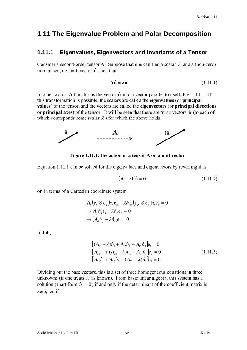
nnA ˆˆ (1.11.1) In other words, A transforms the vector n̂ into a vector parallel to itself, Fig. 1.11.1. If this transformation is possible, the scalars are called the eigenvalues (or principal values) of the tensor, and the vectors are called the eigenvectors (or principal directions or principal axes) of the tensor. It will be seen that there are three vectors n̂ (to each of which corresponds some scalar ) for which the above holds.

Figure 1.11.1: the action of a tensor A on a unit vector Equation 1.11.1 can be solved for the eigenvalues and eigenvectors by rewriting it as

0ˆ nIA (1.11.2) or, in terms of a Cartesian coordinate system,

0ˆˆ

0ˆˆ

0ˆˆ

iijij

rrijij

rrqppqkkjiij

nnA

nnA

nnA

e

ee

eeeeee

In full,

0ˆ)(ˆˆ

0ˆˆ)(ˆ

0ˆˆˆ)(

3333232131

2323222121

1313212111

e

e

e

nAnAnA

nAnAnA

nAnAnA

(1.11.3)

Dividing out the base vectors, this is a set of three homogeneous equations in three unknowns (if one treats as known). From basic linear algebra, this system has a solution (apart from 0ˆ in ) if and only if the determinant of the coefficient matrix is

zero, i.e. if

An̂ n̂

Section 1.11


0det)det(

333231

232221

131211

AAA

AAA

AAA

IA (1.11.4)

Evaluating the determinant, one has the following cubic characteristic equation of A,

0IIIIII 23 AAA Tensor Characteristic Equation (1.11.5) where

A

AA

A

A

A

A

det

III

)tr()(tr

II

tr

I

321

2221

21

kjiijk

ijjijjii

ii

AAA

AAAA

A

(1.11.6)

It can be seen that there are three roots 321 ,, , to the characteristic equation. Solving

for , one finds that

321

133221

321

III

II

I

A

A

A

(1.11.7)

The eigenvalues (principal values) i must be independent of any coordinate system and,

from Eqn. 1.11.5, it follows that the functions AAA III,II,I are also independent of any coordinate system. They are called the principal scalar invariants (or simply invariants) of the tensor. Once the eigenvalues are found, the eigenvectors (principal directions) can be found by solving

0ˆ)(ˆˆ

0ˆˆ)(ˆ

0ˆˆˆ)(

333232131

323222121

313212111

nAnAnA

nAnAnA

nAnAnA

(1.11.8)

for the three components of the principal direction vector 321 ˆ,ˆ,ˆ nnn , in addition to the

condition that 1ˆˆˆˆ ii nnnn . There will be three vectors iin en ˆˆ , one corresponding to

each of the three principal values. Note: a unit eigenvector n̂ has been used in the above discussion, but any vector parallel to n̂ , for example n̂ , is also an eigenvector (with the same eigenvalue ):

ˆ ˆ ˆ ˆ A n An n n

Section 1.11


Example (of Eigenvalues and Eigenvectors of a Tensor) A second order tensor T is given with respect to the axes 321 xxOx by the values

1120

1260

005

ijTT .

Determine (a) the principal values, (b) the principal directions (and sketch them). Solution: (a) The principal values are the solution to the characteristic equation

0)15)(5)(10(

1120

1260

005

which yields the three principal values 15,5,10 321 .

(b) The eigenvectors are now obtained from 0 jijij nT . First, for 101 ,

09120

012160

0005

321

321

321

nnn

nnn

nnn

and using also the equation 1ii nn leads to 321 )5/4()5/3(ˆ een . Similarly, for

52 and 153 , one has, respectively,

04120

012110

0000

321

321

321

nnn

nnn

nnn

and

016120

01290

00020

321

321

321

nnn

nnn

nnn

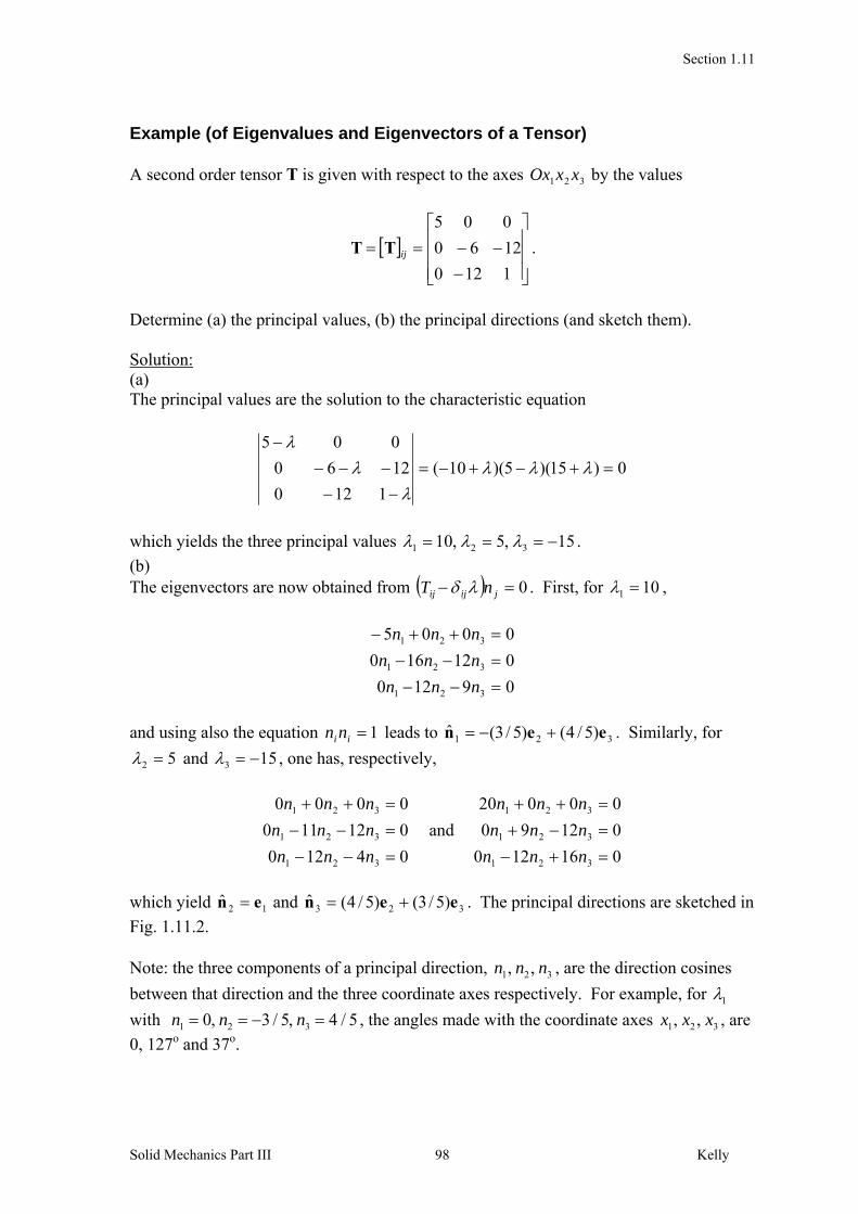
which yield 12ˆ en and 323 )5/3()5/4(ˆ een . The principal directions are sketched in

Fig. 1.11.2. Note: the three components of a principal direction, 1 2 3, ,n n n , are the direction cosines

between that direction and the three coordinate axes respectively. For example, for 1

with 1 2 30, 3 / 5, 4 / 5n n n , the angles made with the coordinate axes 1 2 3, ,x x x , are

0, 127o and 37o.

Section 1.11


Figure 1.11.2: eigenvectors of the tensor T ■

1.11.2 Real Symmetric Tensors Suppose now that A is a real symmetric tensor (real meaning that its components are real). In that case it can be proved (see below) that1

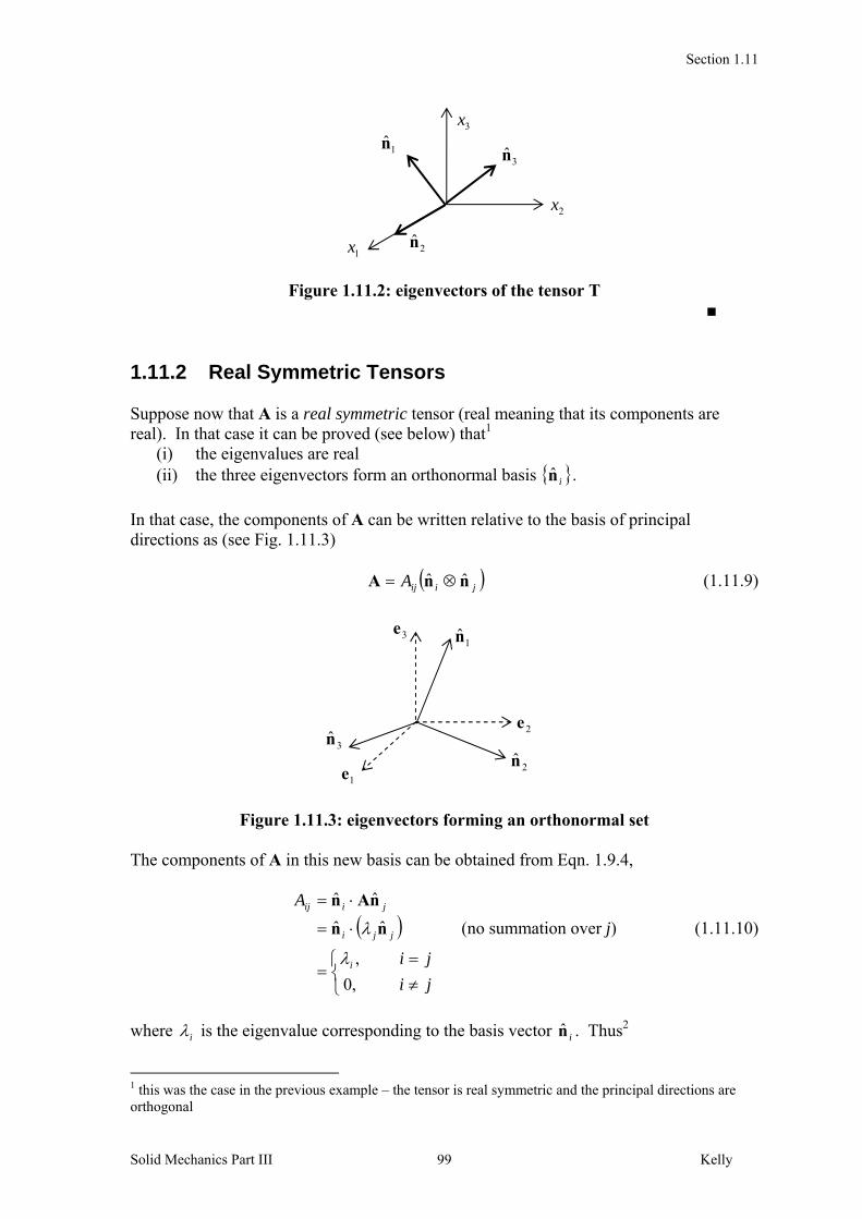
(i) the eigenvalues are real (ii) the three eigenvectors form an orthonormal basis in̂ .

In that case, the components of A can be written relative to the basis of principal directions as (see Fig. 1.11.3)

jiijA nnA ˆˆ (1.11.9)

Figure 1.11.3: eigenvectors forming an orthonormal set The components of A in this new basis can be obtained from Eqn. 1.9.4,

ji

ji

A

i

jji

jiij

,0

,

ˆˆ

ˆˆ

nn

nAn

(no summation over j) (1.11.10)

where i is the eigenvalue corresponding to the basis vector in̂ . Thus2

1 this was the case in the previous example – the tensor is real symmetric and the principal directions are orthogonal

1n̂

2n̂3n̂

1e

2e

3e

3x

1x

2x

3n̂1n̂

2n̂

Section 1.11


3

1

ˆˆi

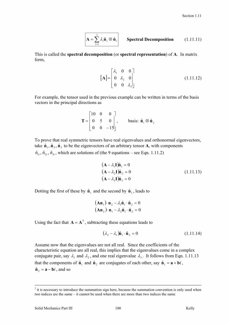
iii nnA Spectral Decomposition (1.11.11)

This is called the spectral decomposition (or spectral representation) of A. In matrix form,

3

2

1

00

00

00

A (1.11.12)

For example, the tensor used in the previous example can be written in terms of the basis vectors in the principal directions as

1500

050

0010

T , basis: ji nn ˆˆ

To prove that real symmetric tensors have real eigenvalues and orthonormal eigenvectors, take 321 ˆ,ˆ,ˆ nnn to be the eigenvectors of an arbitrary tensor A, with components

iii nnn 321 ˆ,ˆ,ˆ , which are solutions of (the 9 equations – see Eqn. 1.11.2)

0ˆ

0ˆ

0ˆ

33

22

11

nIA

nIA

nIA

(1.11.13)

Dotting the first of these by 1n̂ and the second by 1n̂ , leads to

0ˆˆ

0ˆˆ

21212

21121

nnnAn

nnnAn

Using the fact that TA A , subtracting these equations leads to

0ˆˆ 2112 nn (1.11.14) Assume now that the eigenvalues are not all real. Since the coefficients of the characteristic equation are all real, this implies that the eigenvalues come in a complex conjugate pair, say 1 and 2 , and one real eigenvalue 3 . It follows from Eqn. 1.11.13

that the components of 1n̂ and 2n̂ are conjugates of each other, say iban 1ˆ ,

iban 2ˆ , and so

2 it is necessary to introduce the summation sign here, because the summation convention is only used when two indices are the same – it cannot be used when there are more than two indices the same

Section 1.11


0ˆˆ 22

21 bababann ii

It follows from 1.11.14 that 012 which is a contradiction, since this cannot be true for conjugate pairs. Thus the original assumption regarding complex roots must be false and the eigenvalues are all real. With three distinct eigenvalues, Eqn. 1.11.14 (and similar) show that the eigenvectors form an orthonormal set. When the eigenvalues are not distinct, more than one set of eigenvectors may be taken to form an orthonormal set (see the next subsection). Equal Eigenvalues There are some special tensors for which two or three of the principal directions are equal. When all three are equal, 321 , one has IA , and the tensor is

spherical: every direction is a principal direction, since nnInA ˆˆˆ for all n̂ . When two of the eigenvalues are equal, one of the eigenvectors will be unique but the other two directions will be arbitrary – one can choose any two principal directions in the plane perpendicular to the uniquely determined direction, in order to form an orthonormal set. Eigenvalues and Positive Definite Tensors Since nnA ˆˆ , then nnnAn ˆˆˆˆ . Thus if A is positive definite, Eqn. 1.10.38, the eigenvalues are all positive. In fact, it can be shown that a tensor is positive definite if and only if its symmetric part has all positive eigenvalues. Note: if there exists a non-zero eigenvector corresponding to a zero eigenvalue, then the tensor is singular. This is the case for the skew tensor W, which is singular. Since

ωoωωWω 0 (see , §1.10.11), the axial vector ω is an eigenvector corresponding to a zero eigenvalue of W. 1.11.3 Maximum and Minimum Values The diagonal components of a tensor A, 332211, AAA , have different values in different

coordinate systems. However, the three eigenvalues include the extreme (maximum and minimum) possible values that any of these three components can take, in any coordinate system. To prove this, consider an arbitrary set of unit base vectors 321 ,, eee , other than

the eigenvectors. From Eqn. 1.9.4, the components of A in a new coordinate system with these base vectors are jiijA Aee Express 1e using the eigenvectors as a basis,

3211 ˆˆˆ nnne

Then

Section 1.11


32

22

12

3

2

1

11

00

00

00

A

Without loss of generality, let 321 . Then, with 1222 , one has

113

22

21

222233

1132

22

12222

11

A

A

which proves that the eigenvalues include the largest and smallest possible diagonal element of A. 1.11.4 The Cayley-Hamilton Theorem The Cayley-Hamilton theorem states that a tensor A (not necessarily symmetric) satisfies its own characteristic equation 1.11.5:

0IAAA AAA IIIIII 23 (1.11.15) This can be proved as follows: one has nnA ˆˆ , where is an eigenvalue of A and n̂ is the corresponding eigenvector. A repeated application of A to this equation leads to

nnA ˆˆ nn . Multiplying 1.11.5 by n̂ then leads to 1.11.15. The third invariant in Eqn. 1.11.6 can now be written in terms of traces by a double contraction of the Cayley-Hamilton equation with I, and by using the definition of the trace, Eqn.1.10.6:

3

212

233

31

222123

23

23

)tr(trtrtrIII

0III3trtr)tr(trtrtr

0III3trIItrItr

0:III:II:I:

AAAA

AAAAAA

AAA

IIIAIAIA

A

A

AAA

AAA

(1.11.16)

The three invariants of a tensor can now be listed as

3

212

233

31

2221

)tr(trtrtrIII

)tr()(trII

trI

AAAA

AA

A

A

A

A

Invariants of a Tensor (1.11.17)

The Deviatoric Tensor Denote the eigenvalues of the deviatoric tensor devA, Eqn. 1.10.36, 321 ,, sss and the

principal scalar invariants by 321 ,, JJJ . The characteristic equation analogous to Eqn.

1.11.5 is then

Section 1.11


032

21

3 JsJsJs (1.11.18)

and the deviatoric invariants are3

3213

13322122

21

2

3211

devdet

devtrdevtr

)dev(tr

sssJ

ssssssJ

sssJ

A

AA

A

(1.11.19)

From Eqn. 1.10.37,

01 J (1.11.20)

The second invariant can also be expressed in the useful forms {▲Problem 4}

23

22

212

12 sssJ , (1.11.21)

and, in terms of the eigenvalues of A, {▲Problem 5}

213

232

2212 6

1 J . (1.11.22)

Further, the deviatoric invariants are related to the tensor invariants through {▲Problem 6}

AAAAAA III27III9I2,II3I 3271

32

31

2 JJ (1.11.23)

1.11.5 Coaxial Tensors Two tensors are coaxial if they have the same eigenvectors. It can be shown that a necessary and sufficient condition that two tensors A and B be coaxial is that their simple contraction is commutative, BAAB . Since for a tensor T, TTTT 11 , a tensor and its inverse are coaxial and have the same eigenvectors.

3 there is a convention (adhered to by most authors) to write the characteristic equation for a general tensor

with a AII term and that for a deviatoric tensor with a sJ 2 term (which ensures that 02 J - see

1.11.22 below) ; this means that the formulae for J2 in Eqn. 1.11.19 are the negative of those for AII in

Eqn. 1.11.6

Section 1.11


1.11.6 Fractional Powers of Tensors Integer powers of tensors were defined in §1.9.2. Fractional powers of tensors can be defined provided the tensor is real, symmetric and positive definite (so that the eigenvalues are all positive). Contracting both sides of nnT ˆˆ with T repeatedly gives ˆ ˆn nT n n . It follows that, if T has eigenvectors in̂ and corresponding eigenvalues i , then nT is coaxial, having the

same eigenvectors, but corresponding eigenvalues ni . Because of this, fractional powers

of tensors are defined as follows: mT , where m is any real number, is that tensor which has the same eigenvectors as T but which has corresponding eigenvalues m

i . For

example, the square root of the positive definite tensor

3

1

ˆˆi

iii nnT is

3

1

2/1 ˆˆi

iii nnT (1.11.24)

and the inverse is

3

1

1 ˆˆ)/1(i

iii nnT (1.11.25)

These new tensors are also positive definite. 1.11.7 Polar Decomposition of Tensors Any (non-singular second-order) tensor F can be split up multiplicatively into an arbitrary proper orthogonal tensor R ( IRR T , 1det R ) and a tensor U as follows:

RUF Polar Decomposition (1.11.26) The consequence of this is that any transformation of a vector a according to Fa can be decomposed into two transformations, one involving a transformation U, followed by a rotation R. The decomposition is not, in general, unique; one can often find more than one orthogonal tensor R which will satisfy the above relation. In practice, R is chosen such that U is symmetric. To this end, consider FFT . Since

02T FvFvFvFvFv ,

FFT is positive definite. Further, jkji FFFFT is clearly symmetric, i.e. the same result

is obtained upon an interchange of i and k. Thus the square-root of FFT can be taken: let U in 1.11.26 be given by

Section 1.11


2/1TFFU (1.11.27) and U is also symmetric positive definite. Then, with 1.10.3e,

I

UUUU

FUFU

FUFURR

1T

1TT

1T1T

(1.11.28)

Thus if U is symmetric, R is orthogonal. Further, from (1.10.16a,b) and (1.100.18d),

FU detdet and 1det/detdet UFR so that R is proper orthogonal. It can also be proved that this decomposition is unique. An alternative decomposition is given by

VRF (1.11.29) Again, this decomposition is unique and R is proper orthogonal, this time with

2/1TFFV (1.11.30) 1.11.8 Problems 1. Find the eigenvalues, (normalised) eigenvectors and principal invariants of

1221 eeeeIT 2. Derive the spectral decomposition 1.11.11 by writing the identity tensor as

ii nnI ˆˆ , and writing AIA . [Hint: in̂ is an eigenvector.]

3. Derive the characteristic equation and Cayley-Hamilton equation for a 2-D space. Let

A be a second order tensor with square root AS . By using the Cayley-Hamilton equation for S, and relating SS tr,det to AA tr,det through the corresponding

eigenvalues, show that AA

IAAA

det2tr

det

.

4. The second invariant of a deviatoric tensor is given by Eqn. 1.11.19b, 1332212 ssssssJ

By squaring the relation 03211 sssJ , derive Eqn. 1.11.21,

23

22

212

12 sssJ

5. Use Eqns. 1.11.21 (and your work from Problem 4) and the fact that 2121 ss , etc. to derive Eqn. 1.11.22.

6. Use the fact that 0321 sss to show that

Section 1.11


3133221321

2133221

)(III

3)(II

3I

mm

m

m

sssssssss

ssssss

A

A

A

where iim A31 . Hence derive Eqns. 1.11.23.

7. Consider the tensor

100

011

022

F

(a) Verify that the polar decomposition for F is RUF where

100

02/12/1

02/12/1

R ,

100

02/32/1

02/12/3

U

(verify that R is proper orthogonal). (b) Evaluate FbFa, , where T]0,1,1[a , T]0,1,0[b by evaluating the individual

transformations UbUa, followed by UbRUaR , . Sketch the vectors and their images. Note how R rotates the vectors into their final positions. Why does U only stretch a but stretches and rotates b?

(c) Evaluate the eigenvalues i and eigenvectors in̂ of the tensor FFT . Hence

determine the spectral decomposition (diagonal matrix representation) of FFT .

Hence evaluate FFU T with respect to the basis in̂ – again, this will be a

diagonal matrix.

eigen values and polar decomposition

Documents