eirik falck da silva - ntnufolk.ntnu.no/haugwarb/kp8108/essays/eirik_falck_da_silva.pdf · eirik...

Modelling of activity coefficents by comp. chem. 1

Modelling of activity coefficients using computationalchemistry

Eirik Falck da Silva

Report in DIK 2099Faselikevekter

June 2002


SUMMARY ......................................................................................................3

INTRODUCTION .............................................................................................3

background .............................................................................................................................................3

The use of computational chemistry .....................................................................................................4

REVIEW...........................................................................................................4

Introduction ............................................................................................................................................4

Free energy of solvation .........................................................................................................................5Cosmo-RS ............................................................................................................................................7SMx models..........................................................................................................................................7Application of infinite dilution solvation energy..................................................................................8

Equation of state (EOS) approaches .....................................................................................................8UNIQUAC............................................................................................................................................8UNIFAC .............................................................................................................................................10General issues.....................................................................................................................................10Direct approaches ...............................................................................................................................11Indirect methods .................................................................................................................................11

Explicit solvent modelling ....................................................................................................................12

RESULTS AND PROPOSED PROCEDURES..............................................13

Activity coefficients predicted with free energy of solvation ............................................................13

UNIQUAC parameters from Sandlers method..................................................................................14

Ab Initio Fitting to UNIFAC parameters ...........................................................................................15

Monte Carlo modelling of UNIFAC parameters ...............................................................................17

DISCUSSION ................................................................................................21

CONCLUSION...............................................................................................22

LITERATURE ................................................................................................24

APPENDIX 1 .................................................................................................26

APPENDIX 2 .................................................................................................29

APPENDIX 3 .................................................................................................30

APPENDIX 4 .................................................................................................32


Summary

In this work I have looked at various approaches to the estimation of activitycoefficients by computational methods. I have worked on binary systems consisting ofneutral molecules.

I have looked at several approaches described in the literature. Some I onlydiscuss briefly, while others I have studied and applied. I have focused mostly onusing computational methods to obtain parameters for the UNIQUAC and UNIFACequations.

Use of Monte Carlo modelling to obtain energy parameters for UNIQUAC hasbeen fairly successful, supporting an interpretation of UNIQUAC energy parametersas a residual form of the free-energy of solvation.

Introduction

background

My group is working on the processes of CO2 removal from exhaust gases. We arelooking at processes using chemical absorption of CO2 from a gas phase into a liquidphase. In order to understand, control and improve on the absorption process adetailed understanding of the chemistry is necessary. This understanding shouldinclude a model for the activities in the liquid phase.

Use of models such as UNIFAC and UNIQUAC on these absorption processeshas been reported in literature1,2. Published data does not seem to be very reliable andthere is no consistency in reported data. The uncertainty is not surprising since almostall of the work is based on limited experimental data. Often only temperature,pressure, the partial pressure of CO2 and initial concentration of different species inthe system is known. Concentration of various species are often unknown and eventhe understanding of the reaction chemistry can be limited.

Various assumptions must be made and the activity coefficients are only oneof a larger set of properties that must be fitted to the data.

Group contribution models such as UNIFAC can be used, but their reliabilityfor the systems in question is unknown and the group contribution factors available tous do not cover all molecules formed.

Any form of modelling that can generate independent estimates of the activitycoefficients would obviously be useful to improve the understanding and modelling ofthe absorption processes.

The main goal of my own work is to predict the performance of new absorbersfor these processes. A predictive model for the activity of these new absorbers is thendesirable.


The use of computational chemistry

Computational chemistry is a term used to refer to molecular Monte Carlo methods,molecular dynamics and the so called "Ab Initio" methods, based on solving some(simplified) form of the Schrødinger equation.

All these methods are well established. Ab Initio methods have been verysuccessful in modelling of molecular geometry, particularly in the gas-phase. Mostmolecular properties can be calculated with reasonable precision using these methods.

The behaviour of a liquid mixture is a function of molecular properties and itis therefore natural to ask if computational chemistry can not be used to modelactivity in solvents.

While I have not found much work on the modelling of activity in theliterature, modelling of solvation effects is a major topic in computational chemistry.The methods in use can be used to calculate activities and use theory and conceptsthat would seem applicable to overall activity modelling.

Review

Introduction

Activity coefficients are defined as the ratio between activity and some measure of theconcentration, often the mole fraction. Relating this to the chemical potential we get:

)ln(0�� xRT�� 1

It is usual to relate activity to the excess Gibbs energy, defined as:

x)and PT,at solution (ideal x)and PT,at solution ( G - actualE GG � 2

Using this we get that:

)ln(,,

inPTi

E

RTNG

j

��

��

�

�

� 3

Borrowing from Tomasi et al3 we can divide the approaches to modelling activity intothree categories:

� Methods based on the continuum model.

� Elaboration of physical functionals, here we find models such as UNIQUAC andNRTL.

� Methods based on computational simulations of liquids.


While I will not go further into this approach I will finally mention the possibility ofusing quantum chemical descriptors and using statistical methods to find theircorrelation with activity4.

I will discuss these various approaches and their application. Tomasi did note that thedivision of these methods was slightly dated since there was a convergence of thesemethods taking place and in this work I will also show possible combinations of thesemethods.

Free energy of solvation

One quantity often used in computational chemistry is the free energy of solvation(�Gsol), giving the energy in going from (ideal) gas phase to a given solvent phase.If we can calculate �Gsol for two solvent states, we in fact have data to calculateequation 1, i.e. differences in solvation free energy between two systems with thesame reference state (gas-phase) is equivalent to differences in chemical potential.

One main form of modelling �Gsol is the Continuum models, so called becausethey treat the solvent as a continuum. The solvated molecule is placed in a cavity andthe solvent effects are represented by the interaction with the cavity wall and theimposition of an electrostatic field.

Ben Naim5 has developed the following equation to express the solvationenergy based on statistical mechanics:

��

�

�

��

�

�

�

��

�

�

�

��

�

�� 3

,,

3,,

,,

,, lnln)/(sMsM

gMgM

svibsrot

gvibgrotsol n

nRT

qqqq

RTSMWG 4

The equation is based on separating the process in two parts. First you have the workto move the solute to a fixed point in the solvent W(M/S). The final terms give energycontribution of molecular motion. The q's are microscopic partition functions ofrotation and vibration in the gas phase and solution. nM,g and nM,s are the numericaldensities of M molecules and finally the � are momentum partition functions.

The work to add a molecule M to a fixed point in a solvent ( W(M/S) )can bedecomposed into the following elements.

repdiscavel GGGGSMW ��)/( 5

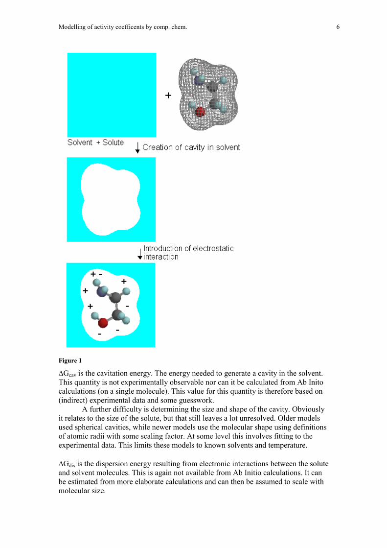
�Gel is the change in the electronic energy of the solute in the presence of theelectrostatic field. This can be computed straight-forwardly in Ab Initio calculations.A general illustration is shown in figure 1.


Figure 1

�Gcav is the cavitation energy. The energy needed to generate a cavity in the solvent.This quantity is not experimentally observable nor can it be calculated from Ab Initocalculations (on a single molecule). This value for this quantity is therefore based on(indirect) experimental data and some guesswork.

A further difficulty is determining the size and shape of the cavity. Obviouslyit relates to the size of the solute, but that still leaves a lot unresolved. Older modelsused spherical cavities, while newer models use the molecular shape using definitionsof atomic radii with some scaling factor. At some level this involves fitting to theexperimental data. This limits these models to known solvents and temperature.

�Gdis is the dispersion energy resulting from electronic interactions between the soluteand solvent molecules. This is again not available from Ab Initio calculations. It canbe estimated from more elaborate calculations and can then be assumed to scale withmolecular size.


�Grep is the repulsion potential. It relates to the quantum mechanical effects of mutualpenetration of electron charge distribution. This presents problems similar to those forthe dispersion energy.

Returning to equation 4 there is still the last two terms. The last term can be viewed asentropy generated by releasing the molecule. While this is a readily calculableproperty it is assumed to be zero in continuum models.

The second term in equation 4 relates to the changes in the internal motions of thesolute as it enters the solvent. The gas-phase motions can be calculated fairly well byAb Initio frequency calculations. There is however at present no models that calculatethis reliably in a solvent. This term will therefore be omitted.

It should be clear from my discussion above that the continuum models are tosome extent based on fitting to experimental data. This suggests that they are lessreliable for untried solvents and their performance outside room temperature is alsounpredictable. It should also be noted that while these models are suited for solvationin pure solvents they can not reliably be extended to other concentrations.

While the continuum models are in wide use there is doubts as to their abilityto model all aspects of solvation. One specific issue is their failure to take account ofhydrogen bonding.

Finally we can note that these models has some similarities with the equationof state approaches to prediction of activity.

Cosmo-RSCosmo-RS6 is a model which is based on the continuum models. The model is basedon calculating a discrete surface around a molecule embedded in virtual conductor.Each surface segment has an area and a so-called screening charge density. A liquid isthen considered as an ensemble of closely packed ideally screened molecules.

Unlike the continuum models this model is able to take account of a solventconsisting of different molecules. The model is a proprietary development, onlyavailable in the commercial Cosmo packages, despite publications on it is difficult tocompare it's performance to that of other models. The problems of determining cavitysizes found in the continuum models would also be present here.

SMx modelsThe SM models are parameterised models for calculating the aqueous free

energies of solvation7. One of the central equations in these models is:

� �� k

kkksol rAG � 6

Here k denotes atom, Ak is the van der Waals surface area and �k is a proportionalityconstant which is referred to as an atomic surface tension. �k is a functional dependenton atomic species. These have been parameterised to experimental data.


This model is simpler and based on a more direct parameterisation then is thecase for continuum models. While less general (it only works for infinite dilution inwater), I have also found it to be precise.

Application of infinite dilution solvation energy

The models above give us solvation energies in infinite dilution, this in itself ishowever not enough to calculate activity coefficients as we do not have a referencestate. Lazaridis8 used the following equation:

� � 02

01,

2,

12

1 lnlnff

kTkT VV��

��

�

�

��

�7

f1 and f2 being the fugacity of the pure components and �V is the residual chemicalpotential relative to an ideal gas mixture. The equation shows the possibility ofcombining relative free energies of solvation (computational) with fugacities of thepure components (experimental data). While this only gives relative activitycoefficients it can also be used to find any single activity coefficient by using thesame species as one of the solutes and solvent.Lazardis applied this equation on Monte Carlo free energy simulations in combinationwith experimental data (to which I will return later). I have tried to do somethingsimilar using the SM model to obtain the free energies of solvation, this work isshown in the results section.

While this method works well it is limited to activity at infinite dilution androom temperature.

Equation of state (EOS) approaches

Before discussing some attempts at using computational methods to give parametersfor equations of state it is appropriate to give a very brief summary of the equations ofstate modelling of activity coefficients.

UNIQUAC

Uniquac9 is one of the classical models for EOS modelling of activity coefficients. Aderivation of the model is given in appendix 1, here I will only summarise the mainfeatures of the equations.

Initially we can note that activity coefficients relate to the excess Gibbs freeenergy (gE) in the following way:

ii

iE

T nRTgn �ln� 8

Where nT is total number of moles.In the UNIQUAC model the excess Gibbs free energy is composed of two parts:


residualE

ialcombinatorEE ggg �� 9

The combinatorial part is the entropy contribution from mixing a set of molecules,while the residual part expresses the energy interactions between different molecularspecies weighted over their surface contact areas.

The following expression were derived for these quantities:

��

��

�

��

��

��

��

�

��

�

2

222

1

111

2

22

1

11 lnln

2lnln

��xqxqz

xx

xx

RTg

ialcombinator

E

10

Where the �'s are local area fractions, i.e. the fraction of area around a species filledby molecules of the same species. � is the total volume fraction of a species. q is thesurface area of a species. z is the coordination number for a molecule, which is simplyassumed to be 10.

� � � �121222212111 lnln ��

��

xqxq

RTg

residual

E

11

Where the � is a expression for molecular interaction energy

��

��

��

��

�

��

��

RTuu jjij

ij exp� 12

Where u is the averaged binding energy for neighbouring molecules.

Finally there is a parameter that I have not shown but that is used in calculating thevolume fraction(�), this is a parameter for molecular size usually written as r.

In the UNIQUAC model the q and r values are general parameters which havebeen calculated for a large number of species. The energy parameters uij and uji arethen fitted to experimental data.

Some attention should be given to the assumptions underpinning UNIQUAC. Thisconcerns the concentration of molecules of different species around one molecules ofone species (�ji - concentration of particles j around species i):

��

��

� ��

RTuu iiji

j

i

ii

ji exp�

�

�

�13

According to this equation the probability that atoms of type i are interacting withmolecules of type j is independent of the interaction between molecules of type j (ujj).If molecules of type j interacted strongly with each other they would be less likely tointeract with molecules of type j and the assumption is therefore wrong. A briefdiscussion on this is given in appendix 4.


The assumption that the interaction parameters are independent of concentration isalso an important assumption and a probably a weakness in the model.

The assumptions regarding mixing can be improved upon quite readily, while a bettermodel of interaction parameters requires a more detailed understanding of molecularinteractions.

A further issue is that in the derivation of UNIQUAC there is assumed to be onlybinary interactions in a liquid. This is a very crude approximation. When fitted toexperimental data it is likely that the energy parameters will also capture these long-range energy contributions, but those contributions do not have the same dependencyon concentrations as assumed in UNIQUAC.

UNIFAC

UNIFAC is a group contribution method. While being based on essentially the samemodel as UNIQUAC it views molecules as a set of groups. By obtaining data for thegroups one would be able to predict the activity of any molecules composed of groupsof which parameters are known. This gives UNIFAC predictive properties thatUNIQUAC does not have.

The main underlying assumptions is that the residual part of of excess gibbsfree energy is a summation over the individual contributions of the groups. This leadsto group energy interaction parameters. The combinatorial energy is calculated usingthe same method as in UNIQUAC, molecular volumes and surfaces being sums ofgroup volumes and surfaces.

The energy of molecular conformers in the solvent phase can vary by severalkcal/mol, especially for large flexible molecules the orientation of the molecule isimportant. This kind of energy contribution can not easily be included in a groupcontribution model, this is one serious short-coming of group contribution models.

In my work I will use UNIFAC with groups corresponding to whole moleculesin which case it is the same as UNIQUAC. I will therefore use these termsinterchangeably.

General issues

All aspects of the UNIQUAC model can be related to concepts and quantities incomputational chemistry. The volumes and areas of species in UNIQUAC can berelated to the cavities used in continuum models and binding energies is somethingreadily available from computational models.

While the UNIQUAC and other EOSs calculation of activity are based onmodels have a physical interpretation but they are in the end fitted to experimentaldata. So it is not clear to what extent the parameters do in fact capture what they wereintended as. This is something that must be kept in mind when combiningcomputational results with these models.


Direct approaches

One of the earlier efforts to use computational chemistry methods to obtainparameters for an EOS (UNIQUAC) was done by Jonsdottir et al10.

They took a straightforward approach. They took the pair of molecules inquestion and used Molecular Mechanics to optimise their interaction. To includetemperature effects the Gibbs free energy was calculated. The energy found here wasthen interpreted as the binding energy in UNIQUAC. While they reported goodresults there seems to be a fundamental flaw in this approach. Say that you had amixture of an alcohol and water. The optimised structure would involve the alcoholfacing the water molecule. Changing the size of the alkane group would not effect thebinding energy to any significant effect. Yet the average binding energy to water mustbe lower for an alcohol with a large alkane group.

A similar approach was described by Sandler11. He used a cluster with 8molecules, 4 of each species. First this cluster was optimised and then molecular pairswere drawn out from the molecular cluster. Binding energies were calculated for thesepairs and the averages of these energies were then used as the parameters inUNIQUAC. Only overall phase-diagrams were shown in Sandlers results, while thesedata seemed good it is difficult to tell from this how good the estimates for the activitycoefficients were. I have attempted to reproduce Sandlers method, details andcomments are given in the result section. Here it will suffice to say that the methodwould seem to suffer from several problems; one thing is that in such a small clusterone would have the same problem as with Jonsdottirs method, poorly binding parts ofa molecule would face out of cluster and not be included in the binding energies.

Indirect methods

Sandler12 proposed a more developed method. First of all not to directly model theparameters in an EOS, but rather to calculate the infinite dilution coefficients and thento use these activity coefficients to fit the UNIQUAC parameters.

His method is fairly elaborate and I will only try to give a summary of theessentials here.

Change in molecular motions upon solvation is ignored in the model, the basicequation being used is:

***chgcavsol GGG �� 14

G* here refers to energy to move to and from fixed points in gasp-phase and solvent.Using the same theory as in equation 2. �Gcav refers to the energy of creating a emptycavity in the solvent, while �Gchg is the energy arising from the insertion of amolecule with electrons and charges in that cavity. This is in itself equivalent toequation number 3 that we encountered in the continuum models. Sandler thencombines the free energies of charging from the continuum models with theUNIQUAC theory, essentially using UNIQUAC to derive the cavitation energy. Theenergy terms in UNIQUAC he is also able to derive from the charging energy fromthe continuum models, most of the volume and area parameters were derived from AbInitio calculations suing van der Waals radius (the exception is water whereUNIQUAC parameters were used).


While Sandler essentially derives the cavitation energy from the UNIQUACmodel, the cavity is still needed in the calculations.

As I mentioned previously the size of the cavities in continuum models are nota priori given. Here Sandler uses van der Waals radius of atoms but adds a scalingfactor . Here an analogy to the UNIFAC method is invoked. The scaling factors aredetermined as a group contribution. All atoms in a group will be given the samescaling factor. These scaling factors are then set by fitting to experimental data foractivity coeffiecents.

While the results presented are very good, most results are reported in terms ofinfinite dilution partition coefficients and average errors for these are reported to be22%, compared with 237% for UNIFAC.

This is however less impressive when one keeps in mind that the model is tosome extent fitted to the same set of experimental data. Furthermore it is noted thatthe results are very sensitive to the setting of the scaling factor.

In the result section I show a less ambitious effort at fitting UNIFACparameters to data from Ab Initio calculations.

Explicit solvent modelling

All methods so far are based on the solvent being treated as a continuum or asgeometrical shapes with some form of electrostatic properties. The other alternative isto explicitly model solute and solvent molecules. The main approaches to doing this isusing molecular dynamics (MD) and Monte Carlo simulations (MC). Both usually usesome potential function to represent molecular interactions. While these models aresimpler then full Ab Initio representations they would present relatively advancedmodels for a solvent system.

When being applied to the modelling of real solvent-solute systems thepotential functions used would rely on some form of parameterisation. But as opposedto what we have seen for other solvent models this would be generalparameterisations.

One general problem with these methods is if one is in fact sampling the entirephase-space, i.e. if one is in fact computing real averages of the properties one islooking at. It is widely thought that properties such as overall energy for a system cannot be calculated accurately. One can however calculate the effects of substituting onemolecule in a system with another. This is usually done by using the Free EnergyPerturbation method, which is based on gradually replacing one molecule by another.

Lazardis et al9 used equation 7 to use free energy perturbations to calculateratio of infinite dilution activity coefficients.

They used a function of the potential energy based on Lennard-Jones andCoulomb potential functions, all with empirically fitted parameters. In their work theyused the Monte Carlo program BOSS13. Their results show quantitative agreementwith experimental data, performing somewhat worse then UNIFAC.

I have used the same kind of calculation to generate parameters for theUNIFAC model. Details and results are shown in result section.

The UNIQUAC model is based on assumptions about the interaction ofmolecules. All these assumptions can to some extent be tested using molecularmodelling. This would however require a more extensive study then I am undertakinghere.


Results and proposed procedures

Activity coefficients predicted with free energy of solvation

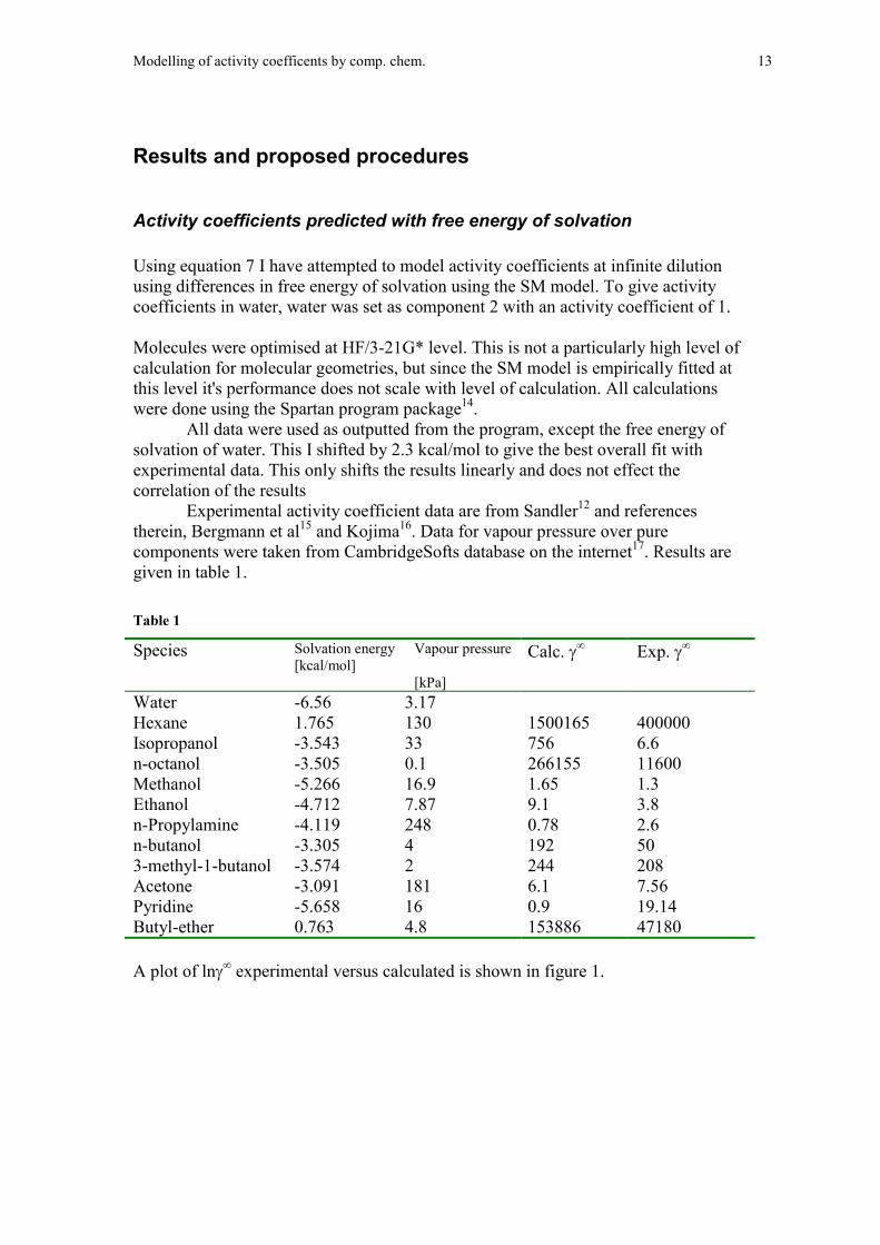
Using equation 7 I have attempted to model activity coefficients at infinite dilutionusing differences in free energy of solvation using the SM model. To give activitycoefficients in water, water was set as component 2 with an activity coefficient of 1.

Molecules were optimised at HF/3-21G* level. This is not a particularly high level ofcalculation for molecular geometries, but since the SM model is empirically fitted atthis level it's performance does not scale with level of calculation. All calculationswere done using the Spartan program package14.

All data were used as outputted from the program, except the free energy ofsolvation of water. This I shifted by 2.3 kcal/mol to give the best overall fit withexperimental data. This only shifts the results linearly and does not effect thecorrelation of the results

Experimental activity coefficient data are from Sandler12 and referencestherein, Bergmann et al15 and Kojima16. Data for vapour pressure over purecomponents were taken from CambridgeSofts database on the internet17. Results aregiven in table 1.

Table 1

Species Solvation energy[kcal/mol]

Vapour pressure

[kPa]

Calc. � Exp. �

Water -6.56 3.17Hexane 1.765 130 1500165 400000Isopropanol -3.543 33 756 6.6n-octanol -3.505 0.1 266155 11600Methanol -5.266 16.9 1.65 1.3Ethanol -4.712 7.87 9.1 3.8n-Propylamine -4.119 248 0.78 2.6n-butanol -3.305 4 192 503-methyl-1-butanol -3.574 2 244 208Acetone -3.091 181 6.1 7.56Pyridine -5.658 16 0.9 19.14Butyl-ether 0.763 4.8 153886 47180

A plot of ln� experimental versus calculated is shown in figure 1.


Figure 2

The overall fit is quite good, especially keeping in mind the very different kind ofmolecules I have looked at. ln-ln plot was partly chosen because of the large spreadin data, but also because in the computational work we are calculating energies anduncertainty in results would be in energy (and proportional to ln).

UNIQUAC parameters from Sandlers method

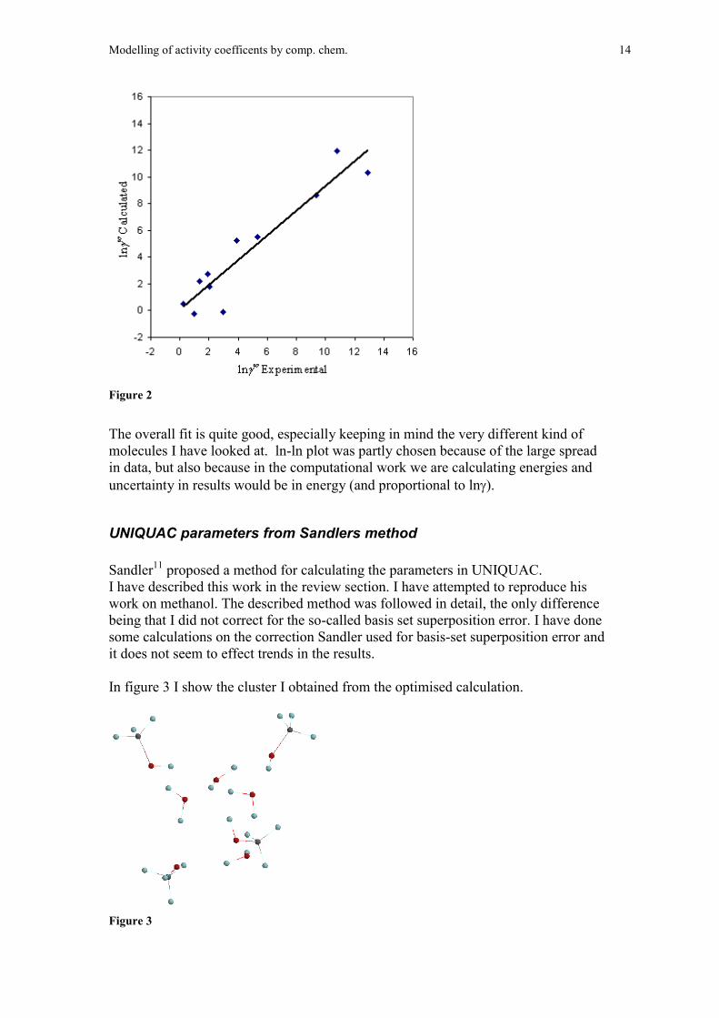
Sandler11 proposed a method for calculating the parameters in UNIQUAC.I have described this work in the review section. I have attempted to reproduce hiswork on methanol. The described method was followed in detail, the only differencebeing that I did not correct for the so-called basis set superposition error. I have donesome calculations on the correction Sandler used for basis-set superposition error andit does not seem to effect trends in the results.

In figure 3 I show the cluster I obtained from the optimised calculation.

Figure 3


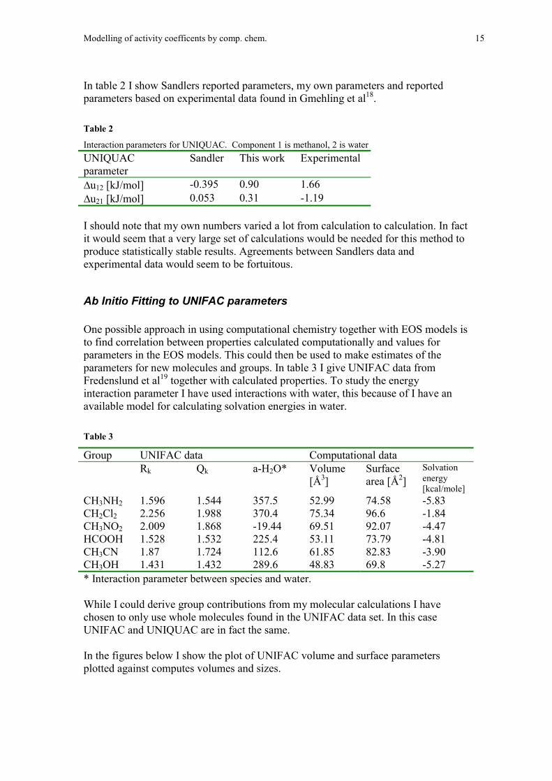
In table 2 I show Sandlers reported parameters, my own parameters and reportedparameters based on experimental data found in Gmehling et al18.

Table 2

Interaction parameters for UNIQUAC. Component 1 is methanol, 2 is waterUNIQUACparameter

Sandler This work Experimental

�u12 [kJ/mol] -0.395 0.90 1.66�u21 [kJ/mol] 0.053 0.31 -1.19

I should note that my own numbers varied a lot from calculation to calculation. In factit would seem that a very large set of calculations would be needed for this method toproduce statistically stable results. Agreements between Sandlers data andexperimental data would seem to be fortuitous.

Ab Initio Fitting to UNIFAC parameters

One possible approach in using computational chemistry together with EOS models isto find correlation between properties calculated computationally and values forparameters in the EOS models. This could then be used to make estimates of theparameters for new molecules and groups. In table 3 I give UNIFAC data fromFredenslund et al19 together with calculated properties. To study the energyinteraction parameter I have used interactions with water, this because of I have anavailable model for calculating solvation energies in water.

Table 3

Group UNIFAC data Computational dataRk Qk a-H2O* Volume

[Å3]Surfacearea [Å2]

Solvationenergy[kcal/mole]

CH3NH2 1.596 1.544 357.5 52.99 74.58 -5.83CH2Cl2 2.256 1.988 370.4 75.34 96.6 -1.84CH3NO2 2.009 1.868 -19.44 69.51 92.07 -4.47HCOOH 1.528 1.532 225.4 53.11 73.79 -4.81CH3CN 1.87 1.724 112.6 61.85 82.83 -3.90CH3OH 1.431 1.432 289.6 48.83 69.8 -5.27* Interaction parameter between species and water.

While I could derive group contributions from my molecular calculations I havechosen to only use whole molecules found in the UNIFAC data set. In this caseUNIFAC and UNIQUAC are in fact the same.

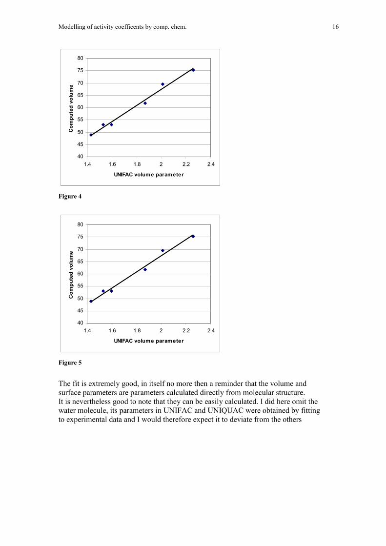
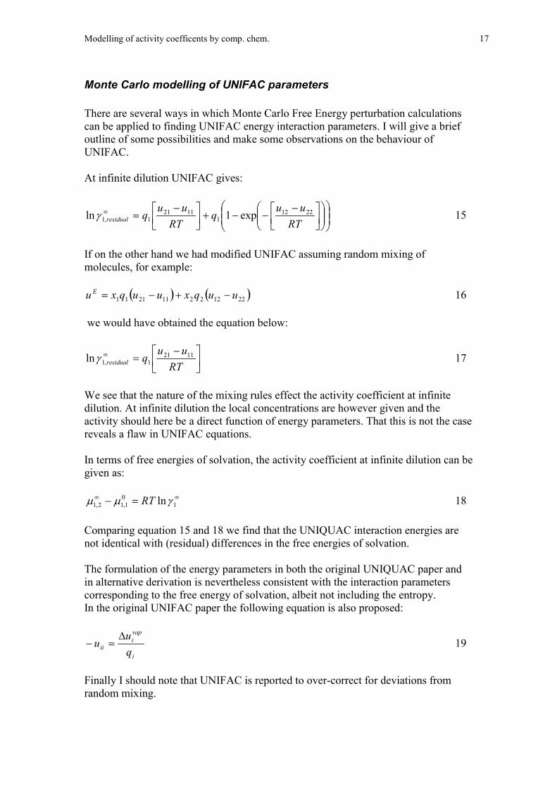
In the figures below I show the plot of UNIFAC volume and surface parametersplotted against computes volumes and sizes.


40

45

50

55

60

65

70

75

80

1.4 1.6 1.8 2 2.2 2.4

UNIFAC volume parameter

Com

pute

d vo

lum

e

Figure 4

40

45

50

55

60

65

70

75

80

1.4 1.6 1.8 2 2.2 2.4

UNIFAC volume parameter

Com

pute

d vo

lum

e

Figure 5

The fit is extremely good, in itself no more then a reminder that the volume andsurface parameters are parameters calculated directly from molecular structure.It is nevertheless good to note that they can be easily calculated. I did here omit thewater molecule, its parameters in UNIFAC and UNIQUAC were obtained by fittingto experimental data and I would therefore expect it to deviate from the others


Monte Carlo modelling of UNIFAC parameters

There are several ways in which Monte Carlo Free Energy perturbation calculationscan be applied to finding UNIFAC energy interaction parameters. I will give a briefoutline of some possibilities and make some observations on the behaviour ofUNIFAC.

At infinite dilution UNIFAC gives:

��

��

��

��

��

�

� ��

�

�

� ��

RTuu

qRT

uuqresidual

22121

11211,1 exp1ln� 15

If on the other hand we had modified UNIFAC assuming random mixing ofmolecules, for example:

� � � �221222112111 uuqxuuqxu E�� 16

we would have obtained the equation below:

��

��

� ��

RTuu

qresidual1121

1,1ln� 17

We see that the nature of the mixing rules effect the activity coefficient at infinitedilution. At infinite dilution the local concentrations are however given and theactivity should here be a direct function of energy parameters. That this is not the casereveals a flaw in UNIFAC equations.

In terms of free energies of solvation, the activity coefficient at infinite dilution can begiven as:

��

�� 101,12,1 ln�� RT 18

Comparing equation 15 and 18 we find that the UNIQUAC interaction energies arenot identical with (residual) differences in the free energies of solvation.

The formulation of the energy parameters in both the original UNIQUAC paper andin alternative derivation is nevertheless consistent with the interaction parameterscorresponding to the free energy of solvation, albeit not including the entropy.In the original UNIFAC paper the following equation is also proposed:

i

vapi

ii qu

u

�� 19

Finally I should note that UNIFAC is reported to over-correct for deviations fromrandom mixing.


The free energy perturbation calculations gives differences in free-energies betweenmolecules in the same solvent. Which means that it can not directly be used to solveequation 18.

It is not clear to what extent the free energy perturbations include entropy effects andI have chosen to interpret them as residual free energies of solvation, i.e. notcontaining entropy.

I have come up with two main ways of using the free energy perturbations to obtainUNIFAC parameters:

We can first use free energy perturbation method to calculate the activity coefficientsat infinite dilution and then set the interaction energy parameters in UNIFAC to givethe same activity coefficients at infinite dilution. This we can do by using equation 7,or borrowing an assumption from UNIFAC:

��

� 1,22,1 �� 20

Using this assumption and equation 18 we get

��

�� 101,11,2 ln�� RT 21

Alternatively we can use the free energies of perturbation directly as interactionparameters. This is the method that seems the most promising and which I will usefrom here on.

Calculations were done using BOSS version 4.3 developed by Professor WilliamJorgensen13. The program uses Lennard-Jones and Coulomb potential functions toexpress the potential energy. These parameters are to some extent empirical in nature.Boxes with 267 solvent molecules were used. All solvent boxes were equilibrated forat least 10 million configurations before use. The perturbation was performed over 5steps, each with 500000 configurations of equilibration and 500000 configurations ofaveraging. Further details are given in Appendix 2.

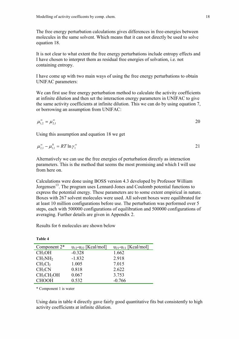
Results for 6 molecules are shown below

Table 4

Component 2* u12-u22 [Kcal/mol] u21-u11 [Kcal/mol]CH3OH -0.328 1.662CH3NH2 -1.832 2.918CH2Cl2 1.005 7.015CH3CN 0.818 2.622CH3CH2OH 0.067 3.753CHOOH 0.532 -0.766* Component 1 is water

Using data in table 4 directly gave fairly good quantitative fits but consistently to highactivity coefficients at infinite dilution.


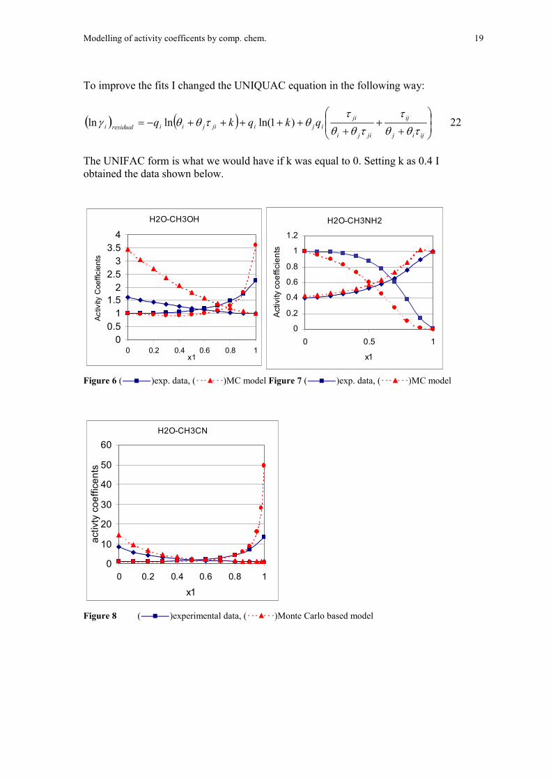
To improve the fits I changed the UNIQUAC equation in the following way:

� � � ��

�

�

��

�

�

��

��

ijij

ij

jiji

jiijijijiiresiduali qkqkq

��

�

��

�� )1ln(lnln 22

The UNIFAC form is what we would have if k was equal to 0. Setting k as 0.4 Iobtained the data shown below.

H2O-CH3OH

00.5

11.5

22.5

33.5

4

0 0.2 0.4 0.6 0.8 1x1

Activ

ity C

oeffi

cien

ts

H2O-CH3NH2

0

0.2

0.4

0.6

0.8

1

1.2

0 0.5 1

x1

Activ

ity c

oeffi

cien

ts

Figure 6 ( )exp. data, ( )MC model Figure 7 ( )exp. data, ( )MC model

H2O-CH3CN

0

10

20

30

40

50

60

0 0.2 0.4 0.6 0.8 1

x1

activ

ty c

oeffi

cent

s

Figure 8 ( )experimental data, ( )Monte Carlo based model


H2O CH2Cl2

0

50

100

150

200

250

300

0 0.2 0.4 0.6 0.8 1x 1

Act

ivity

coe

ffic

ient

s

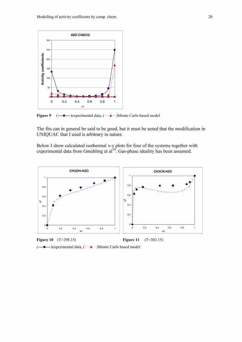
Figure 9 ( )experimental data, ( )Monte Carlo based model

The fits can in general be said to be good, but it must be noted that the modification inUNIQUAC that I used is arbitrary in nature.

Below I show calculated isothermal x-y plots for four of the systems together withexperimental data from Gmehling et al18. Gas-phase ideality has been assumed.

CH3OH-H2O

0

0.2

0.4

0.6

0.8

1

0 0.2 0.4 0.6 0.8 1x1

y1

CH3CN-H2O

0

0.2

0.4

0.6

0.8

1

0 0.2 0.4 0.6 0.8 1x1

y1

Figure 10 (T=298.15) Figure 11 (T=303.15)

( )experimental data, ( )Monte Carlo based model


H2O-CHOOH

0

0.2

0.4

0.6

0.8

1

0 0.2 0.4 0.6 0.8 1x 1

CH3CH2OH-H2O

0

0.2

0.4

0.6

0.8

1

0 0.2 0.4 0.6 0.8 1x1

y1

Figure 12 (T=298.14) Figure 13 (T=303.15)

( )experimental data, ( )Monte Carlo based model

The overall quality of the results must be said to be fairly good. The computationalparameters showing overall quantitative agreement with UNIQUAC parameters andexperimental data. The only result that is rather poor is the data for ethanol, but evenhere we find some quantitative agreement with experimental data.

It should here be noted that water, methanol (CH3OH) and acetonitrile(CH3CN) have been parameterised as solvents in BOSS, while for formic acid andethanol I had to create the solvent input myself. The relatively poor performance forthese molecules might reflect that the solvent molecule parameters are not as carefullyset and also the fact that these molecules are slightly more complex and thereforemore difficult to model accurately.

What can be seen from the plots is that the fits are quite good at low/highconcentrations and poorer fit at molar ratios of 1:1. This is not surprising when weconsider that the energy parameters were estimated at infinite dilution.

Considering the case of ethanol: We measure the interaction parameter withwater at infinite dilution. Under this conditions the alkane group of ethanol will beexposed to water, contributing to a low overall interaction energy. At othercompositions we expect the alkane groups of the ethanol molecules to interact witheach other leaving to the water molecules to interact with the OH groups, therebygiving much stronger interaction.

This explanation does account for the nature of the deviations we see forethanol. This problem is not easily handled in the present model where the energyparameters are assumed to be constant.

Considering the relatively simple molecular representation used in themodelling, this is maybe as good results as one can hope for with the present models.

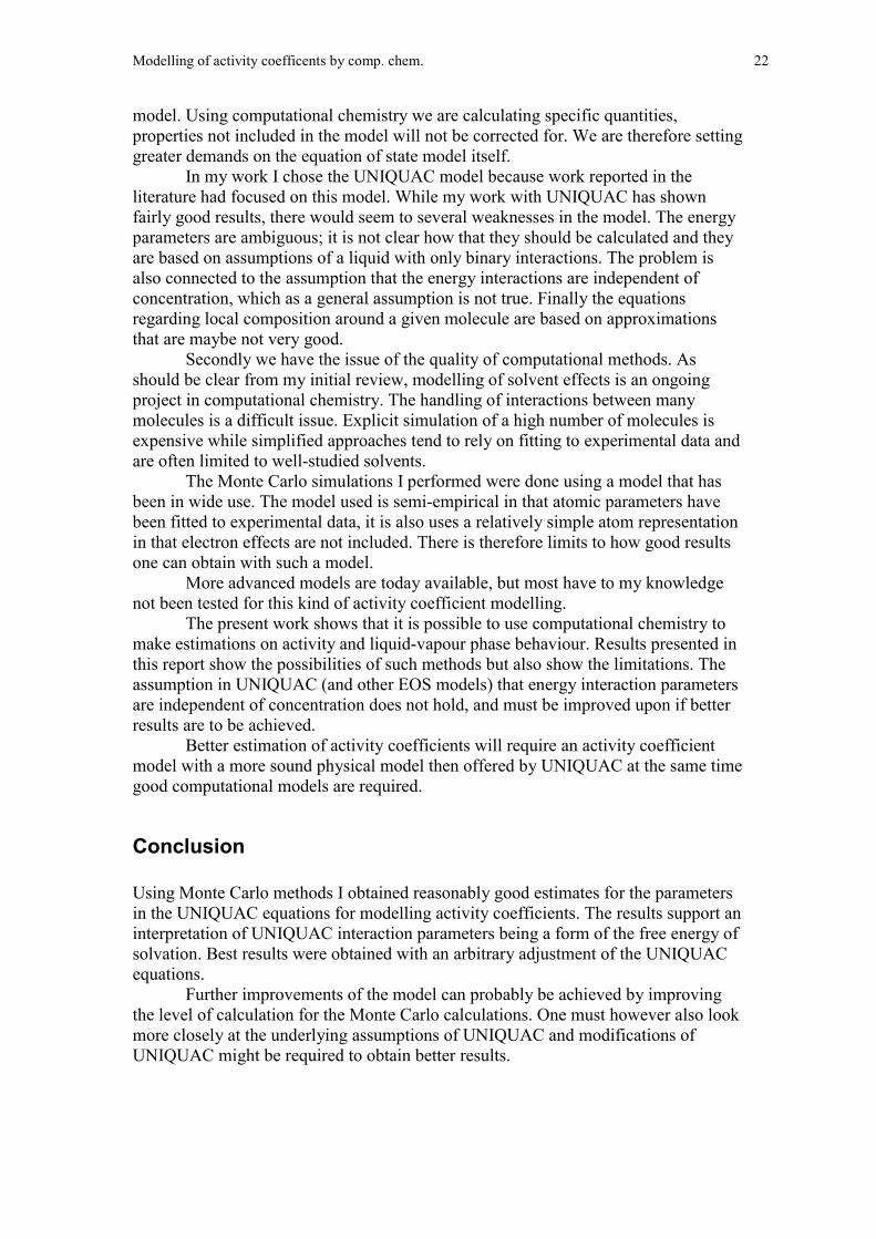
Discussion

In this work I have looked at using computational chemistry methods to generateparameters for equation of state models. There are two main challenges in succeedingwith this. One issue is the equation of state models themselves.

When the equation of state models are used together with experimental data,parameters fitted to experimental data can capture behaviour that is not covered in the


model. Using computational chemistry we are calculating specific quantities,properties not included in the model will not be corrected for. We are therefore settinggreater demands on the equation of state model itself.

In my work I chose the UNIQUAC model because work reported in theliterature had focused on this model. While my work with UNIQUAC has shownfairly good results, there would seem to several weaknesses in the model. The energyparameters are ambiguous; it is not clear how that they should be calculated and theyare based on assumptions of a liquid with only binary interactions. The problem isalso connected to the assumption that the energy interactions are independent ofconcentration, which as a general assumption is not true. Finally the equationsregarding local composition around a given molecule are based on approximationsthat are maybe not very good.

Secondly we have the issue of the quality of computational methods. Asshould be clear from my initial review, modelling of solvent effects is an ongoingproject in computational chemistry. The handling of interactions between manymolecules is a difficult issue. Explicit simulation of a high number of molecules isexpensive while simplified approaches tend to rely on fitting to experimental data andare often limited to well-studied solvents.

The Monte Carlo simulations I performed were done using a model that hasbeen in wide use. The model used is semi-empirical in that atomic parameters havebeen fitted to experimental data, it is also uses a relatively simple atom representationin that electron effects are not included. There is therefore limits to how good resultsone can obtain with such a model.

More advanced models are today available, but most have to my knowledgenot been tested for this kind of activity coefficient modelling.

The present work shows that it is possible to use computational chemistry tomake estimations on activity and liquid-vapour phase behaviour. Results presented inthis report show the possibilities of such methods but also show the limitations. Theassumption in UNIQUAC (and other EOS models) that energy interaction parametersare independent of concentration does not hold, and must be improved upon if betterresults are to be achieved.

Better estimation of activity coefficients will require an activity coefficientmodel with a more sound physical model then offered by UNIQUAC at the same timegood computational models are required.

Conclusion

Using Monte Carlo methods I obtained reasonably good estimates for the parametersin the UNIQUAC equations for modelling activity coefficients. The results support aninterpretation of UNIQUAC interaction parameters being a form of the free energy ofsolvation. Best results were obtained with an arbitrary adjustment of the UNIQUACequations.

Further improvements of the model can probably be achieved by improvingthe level of calculation for the Monte Carlo calculations. One must however also lookmore closely at the underlying assumptions of UNIQUAC and modifications ofUNIQUAC might be required to obtain better results.


List of symbolsEquations only appearing in the review section are not covered here

x = liquid-phase mol fractiony = gas-phase mol fraction�ij��ij

�= chemical potential of i at infinite dilution in j�ii��ii

0 = chemical potential of pure component i � = activity coefficientT = temperaturef = fugacityG = Gibbs free energy�

V = �-�Ideal gas mixture(T,x,�)�

Vap = Free energy of vaporisation

in UNIQUAC/UNIFACnT = total number of molesni = moles of component i�i = area fraction�ij = local area fraction of sites belonging to molecule i around sties belonging

to molecule j� = Given by equation 12�i = Segment fraction uij = binary interaction parameterr = pure-component volume parameterq = pure component area parameterz = coordination number for moleculeuE = molar excess energy


Literature

1. Nath, A.,Bender, E. "Isothermal Vapor-Liquid Equilibria of binary and Ternary MixturesContaining Alcohol, Alkanolamine, and Water with a new Static Device" J.Chem. EngData (1983),28, p 370-375

2. Kaewischan, L, Al-Bofersen, O., Yesavage, V. F., Selim, M. S. "Predictions of thesolubility of acid gases in monoethanolamine (MEA) and methyldiethanolamine (MDEA)solutions using the electrolyte-UNIQUAC model. Fluid Phase Equil. , 183, (2001), p159-171

3. Tomasi, J. and Persico, M. , "Molecular Interactions in Solution: An overview of methodsBased on Continuous Distributions of the Solvent", Chem. Rev. 95 (1994), p 2027-2094

4. Delegado, E. J., Alderete, J. B. "Prediction of infinite dilution activity coefficients ofchlorinated organic compounds in aqueous soultion from quantum-chemical descriptors",J. Comp. Chem. 22 (2001), p 1851-1856

5. Ben-Naim, A., "Standard Thermodynamics of transfer. Uses and Misuses,"J.Phys.Chem.,82,(1978),p 792

6. Eckart, F. and Klamt, A. , "Fast Solvent Screening via Quantum Chemistry: COSMO-RSApproach", AIChE J, 48, No. 2 (2000), p 369-385

7. Chambers, C. C. , Hawkins, G. D. , Cramer, C. J., Truhlar, D. G. , " Model for AqueousSolvation Based on Class IV Atomic Charges and First Solvation Shell Effects", J. Phys.Chem. , 100, No 40 (1996), p 16385-16398

8. Lazaridis, T. and Paulaitis, M. E., " Activity Coefficients in Dilute Aqueous Solutionsfrom Free Energy Silmulation", AIChE J., 39 , No 6, (1993) p 1051-1060

9. Abrams, D. S. and Prauznitz, J. M. "Statistical Thermodynamics of Liquid Mixtures: Anew Expression for the Excess Gibbs Energy of Partly or Completely Miscible Systems,"AIChE J., 21 , No 6, (1975) p 116-128

10. Jónsdóttir, S. O., Klein, R. A. , "UNIQUAC Interaction Parameters for Alkane/AmineSystems Determined by Molecular Mechanics"," Fluid Phase Equi. , 115, (1996), p 59

11. Sum, A. K., Sandler, S. I. "Use of Ab Initio methods to make phase equilibria predictionsusing activity coefficient models" Fluid Phase Equi, , 158-160(1999), p 375-380

12. Lin, S-T. and Sandler, S. I., "Infinite Dilution Activity Coefficients from Ab InitioSolvation Calculations," AIChE J., 45, (1999) p 2606-2618

13. Jorgensen, W.L.,BOSS version 4.3, Yale University, New Haven, CT(1989a)

14. PC SPARTAN Version 1.0.7, Wavefuncion, Inc., 18401 Von Karmen Ave. #370 Irvine,CA 92715, USA.

15. Bergmann, D. L. and Eckart, C. A., "Measurement of Limiting Activity Coefficients forAqueous Systems by differential Ebulliometry, " Fluid Phase Equi., 63, 141 (1991)


16. Kojima, K., Zhang, S. and Hiaki, T. , "Measuring Methods of infinite Dilution ActivityCoefficients and a Database for systems including water", Fluid Phase Equi.,131 145(1997)

17. http://chemfinder.cambridgesoft.com/

18. Gmehling, J. Onken, U., Arlt, W. "Vapor-Liquid Equilibrium Data Collection",DECHME, Frankfurt, 1977 and onwards.

19. Fredenslund, A. Ghmeling,J and Rasmussen, P. "Vapor-liquid equilibrium usingUNIFAC" Elsevier, Amsterdam, 1977


Appendix 1 The UNIQUAC equation

Rather then using the original presentation of the UNIQUAC equation, I will here use the onechosen by Prauznitz et al*.

Here I will look at the case of a binary mixture.Surface area of a molecule 1 is given by a paramter q1. The number of interactions is

assumed to be zq1, where z is the coordination number.We consider one molecule of component 1 being isothermally vaporized from its

pure liquid denoted by superscript (0) and then condensed into a fluid mixture (1). We assumethat that a molecule has z(0) nearest neighbours. We assume that intermolecular forces areshort range and therefore only consider nearest neighbour interactions; the energy ofvaporization per molecule is 1/2z(0)U11

(0) where U11(0) characterizes the potential energy of two

nearest neighbours in pure liquid 1.The central molecule in the fluid mixture is surrounded by z(1)

�11 molecules of species1 and z(1)

�21 of species 2, where �11 is the local surface fraction of component 1, about centralmolecule 1, and �21 is the local surface fraction of component 2, about central molecule 1 (Note that �11+�21=1). We now assume z(0) is the same as z(1). The energy released by thecondensation process is 1/2z(�11U11

(1)+ �21U21(1)), where the superscript on z has been

dropped. We make a similar transfer for a molecule 2 from the pure liquid, denoted bysupersicript (0), to a fluid mixture, denoted by superscript (2).

We now consider a mixture of x1 moles of fluid (1) and x2 moles of fluid (2). Fromthe two-fluid theory we have that for extensive configurational properties (M):

)2(2

)1(1 MxMxM mixture �� A1

The total change in energy in transferring x1 moles of species 1 from pure liquid 1 and x2moles of species 2 from pure liquid 2 into the "two-liquid" mixture, i.e., the molar excessenergy uE, is given by:

� �� )0(22

)2(2112

)2(222222

)0(11

)1(2121

)1(111111 2

121 UUUqNzxUUUqNzxu AA

E�� A2

where NA is Avogadro's number. Since the local surface fractions must obey the conservationequations

11

2212

1121

��

��

��

��A3

and assuming that U11(1)=U11

(0) and U22(2)=U22

(0) equation 2 simplifies to

� � � �� 221221221121121121 UUqxUUqxzNu A

E�� A4

where we have now dropped the superscripts. We now assume

� �

��

�

�

��

�

��

�kT

UUz 1121

1

2

11

21 21

exp�

�

�

�A5

*Prausnitz, J., Lichtentaler, R. and Gomes de Azevedo, E. "Molecular thermodynamics of Fluid-Phase Equilibria" third edition, Prentice Hall (1999)


and

� �

��

�

�

��

�

��

�kT

UUz 2212

2

1

22

12 21

exp�

�

�

�

where � is the surface fraction:

2211

111 qxqx

qx�

�� and 2211

222 qxqx

qx�

�� A6

When these assumptions are coupled we obtain:

121222212111 uqxuqxu E�� A7

and

)/exp()/exp(

)/exp()/exp(

1212

12112

2121

21221

RTuRTu

RTuRTu

��

��

��

��

��

��

��

��

A8

where

� � ANUUzu 112121 21

�� and � � ANUUzu 221212 21

��

A9

We use the approximation (aE)T,V�(gE)T,P and use

EE

uTdTad

�

)/1()/(

A10

Solving for gE from equation A7 we get the residual excess free energy:

��

��

��

�

� ��

�

��

��

�

� ��

�

�

�

RTu

qxRT

uqx

RTg

residual

E12

122221

2111 explnexpln �� A11

The entropy contribution is taken from equations by Guggenheim** and is referred to ascombinatoral energy:

��

��

�

��

��

��

��

�

��

�

2

222

1

111

2

22

1

11 lnln

2lnln

��xqxqz

xx

xx

RTg

ialcombinator

E

A12

Where � is the volume fraction

2211

111 rxrx

rx�

�� and 2211

222 rxrx

rx�

�� A13

r being the molecular volumes.

** Guggenheim, E. A:, Mixtures. Oxford: Oxford University Press, 1952.


Using:

inPTi

ET RTngn

j

�ln,,

��

��

�

�

�A14

We finally obtain the expressions for activity coefficents:

� � � ��

�

�

��

�

�

��

��

ijij

ij

jiji

jiijjijiiresiduali qq

��

�

��

�� lnln A15

Where ��

��

��

��

�

��

��

RTuu jjij

ij exp� A16

And

� �

� � � � � � � ��

�

�

��

�

��

��

��

�

�

12

12

ln2

lnln

jjjj

iiiij

i

i

i

iialcombinatori

rqrzrr

rqrz

zx

��

A17


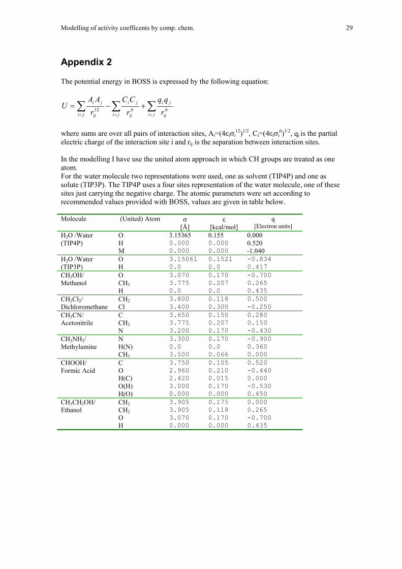
Appendix 2

The potential energy in BOSS is expressed by the following equation:

��

��

ji ij

ji

ji ij

ji

ji ij

ji

rqq

rCC

rAA

U 6612

where sums are over all pairs of interaction sites, Ai=(4�i�i12)1/2, Ci=(4�i�i

6)1/2, qi is the partialelectric charge of the interaction site i and rij is the separation between interaction sites.

In the modelling I have use the united atom approach in which CH groups are treated as oneatom.For the water molecule two representations were used, one as solvent (TIP4P) and one assolute (TIP3P). The TIP4P uses a four sites representation of the water molecule, one of thesesites just carrying the negative charge. The atomic parameters were set according torecommended values provided with BOSS, values are given in table below.

Molecule (United) Atom �

[Å]�

[kcal/mol]q

[Electron units]H2O /Water O 3.15365 0.155 0.000(TIP4P) H 0.000 0.000 0.520

M 0.000 0.000 -1.040H2O /Water O 3.15061 0.1521 -0.834 (TIP3P) H 0.0 0.0 0.417 CH3OH/ O 3.070 0.170 -0.700 Methanol CH3 3.775 0.207 0.265

H 0.0 0.0 0.435 CH2Cl2/ CH2 3.800 0.118 0.500 Dichloromethane Cl 3.400 0.300 -0.250 CH3CN/ C 3.650 0.150 0.280 Acetonitrile CH3 3.775 0.207 0.150

N 3.200 0.170 -0.430 CH3NH2/ N 3.300 0.170 -0.900 Methylamine H(N) 0.0 0.0 0.360

CH3 3.500 0.066 0.000 CHOOH/ C 3.750 0.105 0.520 Formic Acid O 2.960 0.210 -0.440

H(C) 2.420 0.015 0.000 O(H) 3.000 0.170 -0.530 H(O) 0.000 0.000 0.450

CH3CH2OH/ CH3 3.905 0.175 0.000 Ethanol CH2 3.905 0.118 0.265

O 3.070 0.170 -0.700 H 0.000 0.000 0.435


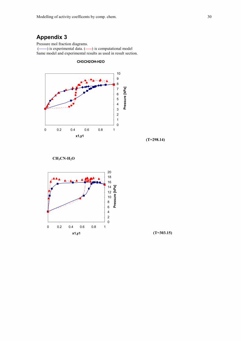
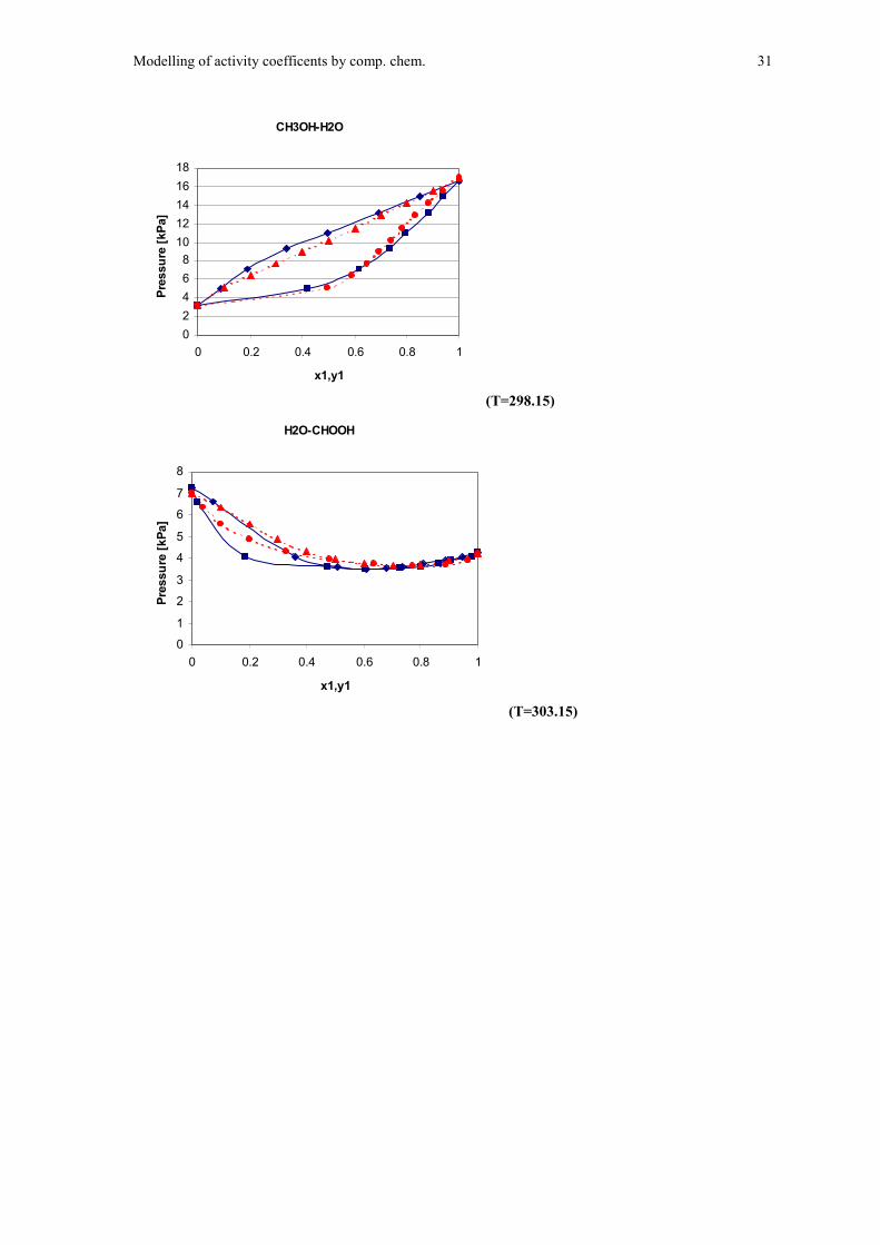
Appendix 3 Pressure mol fraction diagrams. ( ) is experimental data. (-----) is computational modelSame model and experimental results as used in result section.

CH3CH2OH-H2O

012345678910

0 0.2 0.4 0.6 0.8 1

x1,y1

Pres

sure

[kPa

]

(T=298.14)

(T=303.15)

02468101214161820

0 0.2 0.4 0.6 0.8 1

x1,y1

Pres

sure

[kPa

]

CH3CN-H2O


CH3OH-H2O

02468

1012141618

0 0.2 0.4 0.6 0.8 1

x1,y1

Pres

sure

[kPa

]

(T=298.15)

H2O-CHOOH

0

1

2

3

4

5

6

7

8

0 0.2 0.4 0.6 0.8 1

x1,y1

Pres

sure

[kPa

]

(T=303.15)


Appendix 4Rules of mixing

In UNIQUAC the following rules are assumed for mixing:

��

��

� ��

RTuu iiji

j

i

ii

ji exp�

�

�

�1

where �ji is surface fraction of molecule j around central molecule i (as in Appendix 1).

Here I will propose an alternate form for this quantity borrowing from a model developed byPelton and Blander*. In their work they use bondfractions (Xij):

332211 nnnn

X ijij

��

� 2

where nij is number of bonds between molecules of type i and j. I assume that the surface fractions of molecule j around i is proportional to the ratio of bondsof type j-j to bonds of type i-i. The exact form would be:

iiji

jiji XX

X2�

�� 3

In Pelton and Blanders work one thinks of bond forming and breaking as a reaction:

� � � � � �2122211 �� 4 based on this they develop reaction-energy and entropy, and finally also a equilibrium-constant. Using their model and derivations we can write equation 3 as:

� �� 1/2exp411

2

��

�

RTzTXX

X

ji

jji

�� 5

where z is the coordination number of a molecule (as in UNIQUAC) , � is the reactionenthalpy, � is reaction entropy and X are molefractions. The enthalpy is given as:

� �jjiiijA uuuzN

�� 22

� 6

where NA is Avogadros number. Following UNIQUAC I assume the entropy term to be 0.We can then write equation 5 as:

� �� 1/2exp411

2

��

�

RTNuuuXX

X

Ajjiiijji

jji� 7

The corresponding form in UNIQUAC (given in Appendix 1) is:� �� )/5.0exp(

)/5.0exp(RTzNuu

RTzNuu

Aiiijji

Aiiijjji

��

��

�

��

�� 8

When comparing these equations we can assume molar fractions and volume fractions to bethe same. Setting Xi and �j as 1 or 0 we see that both equations do go to 1 and 0, as we wouldexpect them to.If we consider the case of component 1 and 2 being the same ( uij=uii=ujj) the exponentialterms disappear and both functions are reduced to �ji=xj. There are two other examples we canlook at uij>>(uii and ujj) and uij<< (uii and ujj).

*Pelton, A. D., Blander, M. "Thermodynamic Analysis of Ordered Liquid Solutions by a ModifiedQuasichemical Approach-Application to Silicate Slags" Metall. Trans. B, Vol 17B 1986,p 805-815


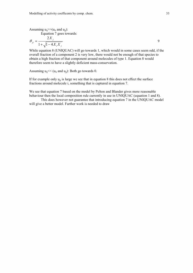
Assuming uij>>(uii and ujj):Equation 7 goes towards:

ji

jji XX

X

411

2

��

�� 9

While equation 8 (UNIQUAC) will go towards 1, which would in some cases seem odd, if theoverall fraction of a component 2 is very low, there would not be enough of that species toobtain a high fraction of that component around molecules of type 1. Equation 8 wouldtherefore seem to have a slightly deficient mass-conservation.

Assuming uij<< (uii and ujj): Both go towards 0.

If for example only ujj is large we see that in equation 8 this does not effect the surfacefractions around molecule i, something that is captured in equation 7.

We see that equation 7 based on the model by Pelton and Blander gives more reasonablebehaviour then the local composition rule currently in use in UNIQUAC (equation 1 and 8).

This does however not guarantee that introducing equation 7 in the UNIQUAC modelwill give a better model. Further work is needed to draw

eirik falck da silva - ntnufolk.ntnu.no/haugwarb/kp8108/essays/eirik_falck_da_silva.pdf · eirik...

Documents