elaborato finale - open-mesh · 2012-03-03 · elaborato finale improving b.a.t.m.a.n. routing...

UNIVERSITA DEGLI STUDI DI TRENTO

Facolta di Scienze Matematiche, Fisiche e Naturali

Corso di Laurea magistrale in Informatica

Elaborato finale

Improving B.A.T.M.A.N.

Routing

Stability and Performance

Relatore: Laureando:

Prof. Renato Lo Cigno Daniele Furlan

Anno Accademico 2010–2011

Abstract

Wireless Mesh Networks (WMN) are diffusing quickly, especially to provide

internet access to area difficult to reach using wired connections, a scenario which

is typical of our region: Trentino in Italy. WMNs are also useful in situations of

public emergency in order to quickly provide connectivity.

WMNs share all the problems widely studied in wired networks, such as con-

gestion control, load balancing and fairness among users. Anyhow these issues in

Wireless Mesh Networks are further complicated because of the nature of wireless

communications that present a number of peculiarities such as significant packet

losses, hidden and exposed terminals problems and stations mobility. These char-

acteristics make solutions studied for wired networks work badly, or not working

at all, in Wireless Mesh Networks.

As a consequence, all the aforementioned questions have to be studied from a

new perspective. One may argue that all of this has already been studied, if not

solved, in MANETs (Mobile Ad-hoc NETworks), however this is not true due

to the different structure, more stable and hierarchical, of WMNs compared to

MANETs.

One of the most notable problems is routing. It has been demonstrated that

traditional hop count routing is sub-optimal in wireless networks, so a great num-

ber of specific routing protocols and metrics have been proposed. In this thesis,

we have chosen to study B.A.T.M.A.N. as routing protocol, because it is one of

the most diffused, and from many real experiments it results to have good per-

formance. Furthermore it is sustained by an active community and has been also

included in the Linux kernel.

This work is a continuation of a previous research project focused on B.A.T.M.A.N.

overhead analysis and on a cross-layer metric improvement [1]. The know-how

gained working on these topics was fundamental to achieve the necessary deep

understanding of the protocol implementation.

In the introductory chapters we provide a general description of Wireless Mesh

Networks from the routing perspective. We briefly list the most important families

of routing protocols, depicting advantages and drawbacks of each solution and

reporting the current open research issues. We continue describing in detail the

B.A.T.M.A.N. routing protocol, reporting its working principles and providing a

list of the most important features.

After the introduction, we provide a formal analysis of the B.A.T.M.A.N.

routing protocol metric, that till now was missing. Starting from the TQ metric

properties, we verify consistency, optimality and loop-freeness of the routing pro-

tocol. We show that the current implementation presents some drawbacks that

can lead to instability and also to the formation of routing loops. We then pro-

pose a modification of the protocol that solves these problems, also providing a

formal proof of loop-freeness that is a crucial property of every routing protocol.

We conclude reporting the results of a number of tests executed using both vir-

tual machines and real devices. Collected data confirm that current B.A.T.M.A.N.

implementation converges slowly in case of node failures due to routing misbe-

haviours, and shows that the proposed modification actually solves these prob-

lems.

Contents

1 Wireless Mesh Networks 1

1.1 WMN architecture . . . . . . . . . . . . . . . . . . . . . . . . . . 1

1.1.1 Node characterization . . . . . . . . . . . . . . . . . . . . 2

1.1.2 Network design . . . . . . . . . . . . . . . . . . . . . . . . 2

1.2 Routing protocols for WMN . . . . . . . . . . . . . . . . . . . . . 3

1.2.1 WMN routing protocol families . . . . . . . . . . . . . . . 4

1.2.2 Types of routing protocols . . . . . . . . . . . . . . . . . . 5

1.3 Routing metrics for WMN . . . . . . . . . . . . . . . . . . . . . . 7

1.3.1 Quality unaware metric . . . . . . . . . . . . . . . . . . . . 7

1.3.2 Quality aware metrics . . . . . . . . . . . . . . . . . . . . 7

2 B.A.T.M.A.N. 11

2.1 The B.A.T.M.A.N. dictionary . . . . . . . . . . . . . . . . . . . . 12

2.2 Originator Messages . . . . . . . . . . . . . . . . . . . . . . . . . 12

2.2.1 OGM flooding . . . . . . . . . . . . . . . . . . . . . . . . . 13

2.2.2 Data structure . . . . . . . . . . . . . . . . . . . . . . . . 13

2.2.3 Local OGM . . . . . . . . . . . . . . . . . . . . . . . . . . 14

2.2.4 Local Link Quality . . . . . . . . . . . . . . . . . . . . . . 15

2.2.5 Path OGM . . . . . . . . . . . . . . . . . . . . . . . . . . 16

2.3 A layer 2 protocol . . . . . . . . . . . . . . . . . . . . . . . . . . . 18

2.3.1 Advantages . . . . . . . . . . . . . . . . . . . . . . . . . . 18

2.3.2 Disadvantages . . . . . . . . . . . . . . . . . . . . . . . . . 19

2.3.3 Other feature . . . . . . . . . . . . . . . . . . . . . . . . . 20

3 B.A.T.M.A.N. is neither optimal nor loop-free 23

3.1 TQ and loss probability . . . . . . . . . . . . . . . . . . . . . . . 23

3.1.1 Local TQ . . . . . . . . . . . . . . . . . . . . . . . . . . . 24

3.1.2 Path TQ . . . . . . . . . . . . . . . . . . . . . . . . . . . . 25

ii CONTENTS

3.2 Routing protocol properties . . . . . . . . . . . . . . . . . . . . . 25

3.2.1 Routing metric and its properties . . . . . . . . . . . . . . 26

3.3 TQ properties, the ideal case . . . . . . . . . . . . . . . . . . . . . 27

3.3.1 Monotonicity . . . . . . . . . . . . . . . . . . . . . . . . . 28

3.3.2 Isotonicity . . . . . . . . . . . . . . . . . . . . . . . . . . . 29

3.3.3 Consistency and optimality . . . . . . . . . . . . . . . . . 30

3.4 The real implementation . . . . . . . . . . . . . . . . . . . . . . . 31

3.4.1 B.A.T.M.A.N. optimality and consistency . . . . . . . . . 31

3.4.2 TQ window and monotonicity violation . . . . . . . . . . . 32

3.4.3 Fast OGM forwarding and loops . . . . . . . . . . . . . . . 34

4 Enforcing loop-freeness for B.A.T.M.A.N. 37

4.1 Assigning zero TQ to lost OGMs . . . . . . . . . . . . . . . . . . 37

4.1.1 Drawbacks . . . . . . . . . . . . . . . . . . . . . . . . . . . 38

4.2 Removing global window and fast OGM forwarding . . . . . . . . 38

4.2.1 Why average is not necessary . . . . . . . . . . . . . . . . 39

4.2.2 Update of path TQ . . . . . . . . . . . . . . . . . . . . . . 39

4.2.3 Route change feasibility . . . . . . . . . . . . . . . . . . . 40

4.2.4 Monotonicity . . . . . . . . . . . . . . . . . . . . . . . . . 41

4.3 Loop-freeness proof . . . . . . . . . . . . . . . . . . . . . . . . . . 41

4.3.1 New OGM fast forwarding . . . . . . . . . . . . . . . . . . 42

5 Results in emulated network and in real test-bed 45

5.1 Test connectivity . . . . . . . . . . . . . . . . . . . . . . . . . . . 46

5.2 Sample run . . . . . . . . . . . . . . . . . . . . . . . . . . . . . . 46

5.3 Convergence time in case of node failure . . . . . . . . . . . . . . 47

5.3.1 Batch means and confidence interval . . . . . . . . . . . . 48

5.3.2 Dependence on TQ GLOBAL WINDOW SIZE . . . . . . 49

5.4 ICMP response percentage . . . . . . . . . . . . . . . . . . . . . . 51

5.4.1 Dependence on TQ GLOBAL WINDOW SIZE . . . . . . 52

5.4.2 Dependence on HOP PENALTY . . . . . . . . . . . . . . 53

5.5 Real test-bed . . . . . . . . . . . . . . . . . . . . . . . . . . . . . 54

5.5.1 Standard B.A.T.M.A.N. convergence time . . . . . . . . . 54

5.5.2 Modified version convergence time . . . . . . . . . . . . . . 55

6 Conclusion 59

CONTENTS iii

A Mesh network emulation 61

A.1 VDE . . . . . . . . . . . . . . . . . . . . . . . . . . . . . . . . . . 61

A.1.1 VDE switch . . . . . . . . . . . . . . . . . . . . . . . . . . 62

A.1.2 VDE plug and wirefilter . . . . . . . . . . . . . . . . . . . 62

A.2 Qemu and OpenWrt . . . . . . . . . . . . . . . . . . . . . . . . . 63

A.3 B.A.T.M.A.N. . . . . . . . . . . . . . . . . . . . . . . . . . . . . . 63

Bibliography 65

iv CONTENTS

Chapter 1

Wireless Mesh Networks

A Wireless Mesh Network (WMN) is a communication network formed by nodes

connected via wireless links. This family of networks differs from ad-hoc networks

because, in the general case, not all nodes are peer one another, but a hierarchi-

cal topology is built based on a given set of node characteristics, e.g. power

availability, dual radio, stability. WMNs differ also from Mobile Ad-hoc Net-

works (MANET) because nodes are typically characterized by reduced or absent

mobility.

Wireless Mesh Networks have a lot of applications, for example they can be

used for providing connectivity in emergency situations, or can be implemented to

provide broadband connectivity to area difficult to reach using wired links, thus

reducing digital divide. WMN are also used in military application to provide

connectivity to units deployed in the battlefield.

Different aspects of WMN have been studied over last years. The main re-

search areas are physical and MAC layer improvements, development of special-

ized routing protocols and application layer support.

In this chapter we give a description of WMN architecture, describing the

current state of the art, focusing on routing protocols. For an exhaustive survey

on WMN the interested reader can refer to [2].

1.1 WMN architecture

Wireless Mesh Network is a definition that includes a family of heterogeneous

networks. Before moving to the routing part, it is necessary to understand how

a WMN can be structured. In fact a routing protocol can be specifically im-

plemented to exploit the characteristics of a given network architecture, or can

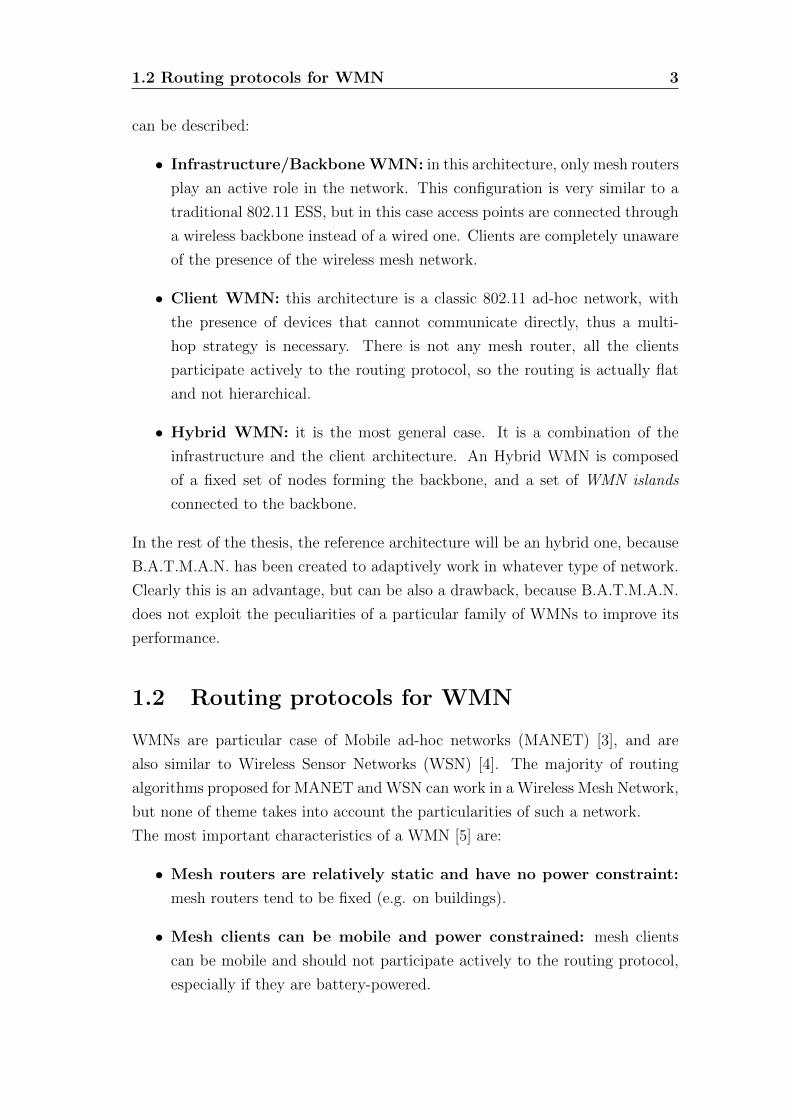
2 Wireless Mesh Networks

Figure 1.1: A typical WMN topology presenting a mix of mesh routers, someof them acting also as gateways toward the Internet, and mesh clients that canbe mesh aware or mesh agnostic.

adaptively work in every different situation.

We start characterizing the nodes in the network dividing theme basing on

their roles. Then we describe the most diffuse types of WMN.

1.1.1 Node characterization

A typical Wireless Mesh Network is depicted in figure 1.1. In a WMN, nodes

can be divided in two categories: mesh routers (or mesh points) and mesh clients

(or mesh stations). Mesh routers typically form the wireless backbone, and can

act as gateways (mesh gateways or mesh portals) toward other networks, usually

providing internet access to the mesh network.

Mesh clients can be further divided in two groups, mesh aware and mesh

agnostic. The first ones participate directly to the routing protocol, the others

are not aware of the existence of the WMN, and are connected to mesh routers

as they were simple access points.

1.1.2 Network design

A WMN can be organized in multiple ways, depending on the purpose of the

network. Basing on the functionality of the nodes, three macroscopic architectures

1.2 Routing protocols for WMN 3

can be described:

• Infrastructure/Backbone WMN: in this architecture, only mesh routers

play an active role in the network. This configuration is very similar to a

traditional 802.11 ESS, but in this case access points are connected through

a wireless backbone instead of a wired one. Clients are completely unaware

of the presence of the wireless mesh network.

• Client WMN: this architecture is a classic 802.11 ad-hoc network, with

the presence of devices that cannot communicate directly, thus a multi-

hop strategy is necessary. There is not any mesh router, all the clients

participate actively to the routing protocol, so the routing is actually flat

and not hierarchical.

• Hybrid WMN: it is the most general case. It is a combination of the

infrastructure and the client architecture. An Hybrid WMN is composed

of a fixed set of nodes forming the backbone, and a set of WMN islands

connected to the backbone.

In the rest of the thesis, the reference architecture will be an hybrid one, because

B.A.T.M.A.N. has been created to adaptively work in whatever type of network.

Clearly this is an advantage, but can be also a drawback, because B.A.T.M.A.N.

does not exploit the peculiarities of a particular family of WMNs to improve its

performance.

1.2 Routing protocols for WMN

WMNs are particular case of Mobile ad-hoc networks (MANET) [3], and are

also similar to Wireless Sensor Networks (WSN) [4]. The majority of routing

algorithms proposed for MANET and WSN can work in a Wireless Mesh Network,

but none of theme takes into account the particularities of such a network.

The most important characteristics of a WMN [5] are:

• Mesh routers are relatively static and have no power constraint:

mesh routers tend to be fixed (e.g. on buildings).

• Mesh clients can be mobile and power constrained: mesh clients

can be mobile and should not participate actively to the routing protocol,

especially if they are battery-powered.


• Mesh routers are frequently equipped with multiple radios: in

presence of multiple wireless interfaces, different strategies can be used to

reduce interferences and/or increase bandwidth.

• Traffic is concentrated along certain paths: most of the traffic origi-

nates or terminates at the gateways.

• Links present non uniform characteristics: wireless links can presents

variable bit-rate, packet loss ratio, etc. It is important to consider these

parameters in routing decisions.

• Network dimension: potentially a WMN is designed to provide connec-

tivity to a large community, so scalability and load balancing are important

features.

It is important for a proper routing protocol to take into account these charac-

teristics, possibly taking advantage from them.

1.2.1 WMN routing protocol families

In the last decade, many algorithms have been proposed specifically for WMN.

They often derive from pre-existing routing algorithms created for MANET and

WSN. Current routing protocols can be divided in three big families: reactive,

proactive and hybrid. We intentionally do not considered static protocols, be-

cause they cannot adapt well to WMN where the network topology and the link

conditions change constantly.

To give a finer taxonomy, according to [2], routing protocols can be classified

basing on their performance optimization objectives. Another possible classifica-

tion, proposed in [6], is based on existing differences in the procedures of route

discovery and maintenance.

Actually it is hard to define a clear taxonomy, because in many case it is

difficult to separate a routing protocol from its routing metric. Indeed in the

cited surveys a routing metric is often reported together with the routing protocol

description.

Reactive protocols

Reactive protocols build a path on demand, reducing the overhead traffic gener-

ated by the routing protocol. This increases scalability and helps reducing power

1.2 Routing protocols for WMN 5

consumption, allowing the protocol to be suitable also for power constrained de-

vices. On the other hand the route establishment phase introduces a delay in the

communication.

The most notable reactive protocols are AODV [7] and DSR [8], which are both

based on flooding for route discovery on demand. The main difference between

the two protocol is that AODV implements hop-by-hop routing while DSR uses

source routing.

Proactive protocols

In contrast to reactive ones, proactive routing protocols, such as OLSR [9], main-

tain current paths towards all the destinations removing any routing establish-

ment delay. Routing information are propagated in the network using flooding,

thus presenting a greater overhead compared to reactive protocols. Scalability is-

sues can be attenuated using particular flooding techniques. Proactive protocols

cannot be used with power constrained devices, because they need continuous

transmission that would rapidly drain the battery.

Hybrid protocols

Another family of routing protocols is called hybrid, and try to mix reactive and

proactive techniques to exploit their advantages and prevent from their draw-

backs. An example of hybrid protocol is HWMP that is the default and required

routing protocol in the IEEE 802.11s [10] definition. It is based on AODV to

establish connections between Mesh Stations, while Mesh Portals maintain up-

to-date routes toward all nodes in a proactive way.

1.2.2 Types of routing protocols

A routing protocol is formed of a path calculation algorithm, that works using a

specific routing metric, and by a packet forwarding scheme, necessary to propa-

gate routing information in the network. We briefly describe the most common

path calculation algorithms and forwarding schemes used in wireless mesh net-

works, listing the main advantages and disadvantages.

After this classification, we can derive for a given protocol, knowing its path

calculation algorithm and its forwarding schema, the necessary formal properties

that a routing metric, used in combination with the protocol, must respect to

guarantee features like loop-freeness, consistency or optimality.


Path calculation algorithms

Path computation algorithms are used to compute the best path toward every

destination according to a certain routing metric. Proactive routing protocols for

WMN, similarly to routing protocols used in wired networks, use the Bellman-

Ford algorithm (distance vector) or the Dijkstra’s algorithm (link state). These

protocols need a constant update of routing information, obtained via periodic

exchange of routing information. This mechanism introduces an overhead that

can become a problem, especially in large ad dense networks. To overcome these

problems, different strategies has been proposed, they consist on reducing the

frequency of updates and/or aggregate them. In OLSR, for example, routing

information are propagated in the network using an optimized flooding technique

based on multipoint relays (MPR) [9] that form a hierarchical logical topology

thus permitting to aggregate routing information.

Reactive routing protocols, on the other hand, use source initiated flooding

to find a suitable route toward a required destination. The overhead in this case

is reduced, because routing frames are sent only when it is needed. The flooding

procedure can also be optimized to further reduce the overhead and speed up the

route discovery process. A similar improvement has been proposed in AODV-ST,

where has been implemented a spanning tree protocol to reduce overhead [11].

Packet forwarding schemes

Two packet forwarding schemes exist, source routing and hop-by-hop routing.

In source routing the entire path (or a unique route sequence number) is

written in each packet header, so every node, upon receiving a packet, essentially

reads the header and forwards the packet accordingly. This scheme is very robust

since it can be easily used to ensure consistency and loop-freeness. The main

drawback is the additional overhead, that anyhow can be reduced using path

sequence numbers as in AODV.

In hop-by-hop routing instead, every node maintains a list of next-hops to-

ward each destination. Packets are forwarded to the current best next-hop until

they reach the final destination. This scheme has much lower overhead, but it is

more prone to problems such as loop formation and slow convergence (counting

to infinity problem). Proper solutions to avoid these problems need to be im-

plemented, especially in case of rapidly changing network conditions, a typical

scenario of networks with mobile devices.

1.3 Routing metrics for WMN 7

1.3 Routing metrics for WMN

A number of metrics have been proposed in the literature, depending on network

characteristics and purposes. For example some routing metrics maximize the sta-

bility of a path considering loss probability, some focus on optimizing throughput

measuring link bandwidth, while others are concerned on energy consumption.

All proposed metrics have both advantages and drawbacks, and adapt well to

specific situations. In any case none of them captures all the important qualities

of a path, and we are still far from the definition of a general metric. This is

probably due to the great number of possible typologies of WMN that in many

cases have specific requirements.

In this section we briefly list the most notable routing metrics for WMN,

dividing them basing on the degree of knowledge of the link characteristics. For

a comprehensive list of routing metrics and their characteristics see [6].

1.3.1 Quality unaware metric

The simplest metric that can be used in WMN is the hop count. This simple met-

ric perform decently in network with high mobility since it rapidly finds available

routes. In more stationary networks, typical of WMN backbones, instead it per-

forms quite bad since it is not able to capture the quality differences between

available paths.

As a consequence, all the links are considered as equal so the path with the

minimum length is chosen. We know that in wireless networks the actual rate

depends on node distance, so it is easy to imagine that choosing long and slow

links, can lead to sub-optimal routing configurations and poor performance.

1.3.2 Quality aware metrics

Quality aware metrics consider the peculiarities of wireless links such as loss

probability, bit-rate and inter and intra-flow interference. Complex metrics often

need a cross layer implementation to access physical layer information. This

approach has been shown to be quite promising for the definition of better WMN

routing metrics [2]. In fact the physical layer is aware of characteristics of wireless

links otherwise difficult to measure at higher layers, such as channel frequency,

physical bit-rate and signal strength.

This approach helps also in presence of mixed wired and wireless links, or in

presence of different types of wireless links (802.11bgn), permitting to distinguish


between interface types thus favouring links with higher capacity and stability.

In this section we briefly list the most common properties of a wireless link,

indicating some of the most diffuse routing metrics proposed in the literature

taking into account these properties.

Link reliability

A first evaluation of link quality can be done measuring link reliability in order

to identify more stable routes. An example is the ML [12] metric which estimates

path loss rate multiplying local link loss probabilities. ETX [13] instead tries to

estimate the expected transmission count, that depends on link reliability since

transmission count increases in case of physical layer retransmission caused by

losses.

Link rate

Those metrics focusing on optimizing the bandwidth have to take into account

the transmission speed of links, that can be time variable. A popular bandwidth

metric is ETT [14] that estimates the expected transmission time of each link

considering also the packet size. ETT is obtained multiplying ETX by the average

packet delivery time. Another notable example is MRS [15], it uses paths having

maximum bit-rate while minimizing transmission power to reduce interferences.

MRS partial experimental results1 are reported in [16] showing an interesting

improvement of measured throughput with respect to ETT.

Interference

Interferences have an huge impact on wireless performance, they can be divided

in intra-flow and inter-flow. Interference is not a local link properties but instead

is influenced by a number of factors that regard the entire path, the network

topology and the traffic load.

Intra-flow interferences are those concerning a single data flow traversing mul-

tiple links sharing the same wireless channel or links using partially overlapping

channels. In this situation we know that each node in the same collision domain

cannot transmit and receive at the same time, and only a node at a time can

transmit. Metrics that consider intra-flow interference are able to favour paths

1Experiment was realizing only with the bit-rate part due to problem dealing with powercontrol on real devices.

1.3 Routing metrics for WMN 9

with the minimum channel share thus increasing the network capacity. An ex-

ample metric is WCETT [14] that combines links ETT in a particular way that

penalizes links sharing the same collision domain.

Inter-flow interference instead is related to concurrent flows sharing the same

wireless resource, and is more difficult to measure as it varies due to network load.

The metric iAWARE [17] attempts to measure interference monitoring signal

to noise ratio (SNR) and signal to interference and noise ratio (SINR) toward

neighbours. Another approach, employed in the MIC [18] metric, is to count the

number of interfering nodes to get an estimation of the inter-flow interference

degree.

Load

An aspect difficult to consider in wireless networks, and also in wired networks,

is link load and load balancing. Implementing routing metrics that consider load

can lead to instability situations and frequent route changes (a phenomena also

known as route flapping).

A notable attempt to consider load in WMN routing is the BLC [19] metric,

which is defined as the minimum residual capacity on a path considering also

its length. Another metric considering link load is the PktPair [20], it measure,

using the packet pair technique, the delay caused by node queuing and channel

occupation, obtaining an estimation of the load along a path.

Chapter 2

B.A.T.M.A.N.

B.A.T.M.A.N. [21] (Better Approach To Mobile Ad-hoc Networking) is a promis-

ing and quite diffuse routing protocol for Wireless Mesh Networks. From real

world experiments it results to have good performance compared to other WMN

routing protocols [22]. It has been also included in the Linux kernel from version

2.6.38, and this fact is a confirmation of the maturity of this project.

B.A.T.M.A.N. belongs to the proactive routing protocols family, and it can be

categorized as a distance-vector routing protocol with an hop-by-hop forwarding

scheme. It is based on a destination initiated periodic flooding of routing man-

agement frames called OGMs (Originator Messages). These packets announce

the presence of the station and are used to discover and maintain routes.

B.A.T.M.A.N. working principle is somehow similar to DSDV [23]. Routing

management frames are marked with unique sequence numbers, both to check

the age of routing information and prevent from the formation of routing loops.

The main difference is that in B.A.T.M.A.N. sequence numbers are independently

applied to each routing table entry, while in DSDV a sequence number identify

the entire routing table. B.A.T.M.A.N. differentiates from DSDV also in route

advertisement frequency, because OGM are sent periodically and not in response

to routing table or topology changes. This is necessary because OGMs are used

also as sample frames to measure the link quality used to calculate the routing

metric.

As a result, every node knows all the other nodes in the network and maintains

a list of available next-hops toward them. The best next-hop, called router, is

chosen accordingly to a path quality metric called TQ (Transmission Quality)

that will be formally described in the next chapter. B.A.T.M.A.N. can also be

used in generic mesh networks with heterogeneous interface typologies, anyhow

12 B.A.T.M.A.N.

the performance of the protocol in this case can be poor because the TQ routing

metric does not distinguish between wired and wireless links nor between fast and

slow links.

2.1 The B.A.T.M.A.N. dictionary

We will use a number of terms specific of the B.A.T.M.A.N. world that are ac-

tually used in the available documentation and also in the source code. In many

cases these terms differ from the ones used in the previous chapter, so before

proceeding in the protocol description, it is necessary to briefly list the specific

terms used to describe the network entities.

• Originator: a node in the network participating actively to the routing

protocol. It has a unique address (level 2) in the network and can have

multiple physical interfaces.

• Neighbour: an originator which is reachable directly (one hop) through

whatever physical interface.

• Router: a candidate neighbour to be next hop toward a specific originator.

The routing protocol identify the best router for each originator according

to a specific metric called TQ.

• Client: a mesh unaware node connected to an originator acting as an access

point or mesh portal.

• Gateway: an originator acting as a gateway toward another network (i.e.

the Internet).

2.2 Originator Messages

The overview of the B.A.T.M.A.N. protocol necessarily starts from the description

of Originator Messages (OGM). They are the core of the protocol, since these

packets are used for neighbour discovery, route information flooding, and lastly

but not least for estimating the quality of links and paths they traverse.

The structure of an OGM is illustrated in figure 2.1. It contains the unique

MAC address of the source station (called Originator), the address of the previous

sender and the Transmission Quality (TQ) of the path it has traversed (set to the

2.2 Originator Messages 13

Figure 2.1: OGM packet structure

maximum value of 255 when the flooding starts). In addition it contains a TTL

field necessary to ensure flooding termination, and a sequence number (SN).

In order to give a more clear description of the protocol, we will logically

divide OGMs in Local and Path OGMs. Local ones are used to compute link

quality, while path OGMs are used to propagate routing informations through

the network.

2.2.1 OGM flooding

OGM flooding is initiated periodically by each originator, that every ORIG -

INTERVAL broadcasts its Originator Message. The packet contains the station

address in the Originator Address field. The TQ value is set to TQ MAX VALUE

that in the current implementation is 255, while the Previous Sender field is left

empty.

Upon the reception of a new OGM (one containing a never seen sequence number),

each station rebroadcast the OGM putting in the TQ field its best TQ toward

the originator. In this way routing information are propagated in the network.

2.2.2 Data structure

The entire protocol depends on the maintenance, in each node, of a set of data

structures that are different for neighbours and originators. For a complete un-

derstating of the mechanisms at the basis of B.A.T.M.A.N. it is necessary to

describe accurately these structures.

Originator data

For each originator O, it is maintained the sequence number SNO of the latest

OGM packet received and a list of available router candidates. A router candidate

is defined as a node from where at least an OGM of O has been received. For

14 B.A.T.M.A.N.

each candidate router Ri(O), it is maintained a sliding window containing the

TQ read in the OGM coming from O and received via Ri. The dimension of the

sliding window is fixed to TQ GLOBAL WINDOW SIZE 1.

The quality of a path is obtained calculating a particular average of the received

TQ values contained in the global window. If a number of OGM equal to TQ -

GLOBAL WINDOW SIZE is not received via a particular candidate router Ri,

its TQ becomes 0 so it is no longer considered as a valid next-hop.

Neighbour data

For each neighbour, are maintained two sliding window of fixed dimension TQ -

LOCAL WINDOW SIZE 2. The first one is used to count the OGM correctly

received from the neighbour, while the second one is necessary to count own OGM

echo received from the neighbour. These local windows are used to estimate the

quality of links toward neighbours. Local link TQs are then combined to obtain

the path quality.

2.2.3 Local OGM

Local OGMs are those used to estimate the quality of a link in term of loss-

probability. They can be divided in:

• Neighbour OGM: OGM of direct neighbour (1-hop neighbours). Previous

sender field is empty.

• Echo OGM: own OGM rebroadcast received from a neighbour. In this

case the previous sender field is equal to receiving station address.

Depending on the type of received OGM, the station behaves differently.

Neighbour OGM

When a station receive an OGM from a neighbour, it does the following opera-

tions:

1. If the station is not known, create a new neighbour entry.

2. If the sequence number is greater that the maximum SN registered for this

neighbour, shift the sliding window accordingly.

1The value of TQ GLOBAL WINDOW SIZE is 5 in the current release.2The value of TQ LOCAL WINDOW SIZE is 64 in the current implementation.


3. Register on the neighbour window the reception of the OGM with the Se-

quence Number contained in the packet.

4. Rebroadcast the OGM updating TQ (see section 2.2.5 for details), reducing

TTL, and replacing previous sender.

Echo OGM

Upon receiving a so called OGM echo, a station perform the following operation:

• Register on the neighbour echo window the reception of the OGM echo with

the Sequence Number contained in SN field.

• Discard the packet.

2.2.4 Local Link Quality

Quality of a local link is estimated indirectly using OGMs received from the

neighbour station. Thanks to sequence numbers, the received OGMs can be

“counted” using a sliding window of fixed dimension TQ LOCAL WINDOW -

SIZE. Receive quality (RQ) is defined as the fraction of OGM received in the

current sliding window.

Clearly it is not sufficient to count the originator messages received, because

we need to estimate the transmission quality (TQ), not the receive quality (RQ)3.

To solve this problem, each node registers, in another similar window, also re-

broadcast of its own OGMs received from the neighbour. In this way a so called

Echo Quality (EQ) is obtained.

Transmission quality of a link from node A to node B can be derived from

RQ and EQ observing that:

EQAB = TQAB ×RQAB

from which it is easy to obtain transmission quality:

TQAB =EQAB

RQAB

The mechanism is schematized in figure 2.2

3In wireless networks, typically links are not symmetric and present different characteristicin the two directions.

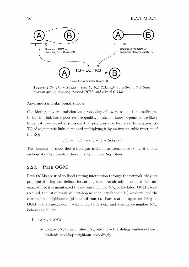
16 B.A.T.M.A.N.

Figure 2.2: The mechanism used by B.A.T.M.A.N. to estimate link trans-mission quality counting received OGMs and echoed OGMs.

Asymmetric links penalization

Considering only transmission loss probability of a wireless link is not sufficient.

In fact if a link has a poor receive quality, physical acknowledgements are likely

to be lost, causing retransmissions that produces a performance degradation. So

TQ of asymmetric links is reduced multiplying it by an inverse cubic function of

the RQ:

TQAB = TQAB ∗ (1− (1−RQAB)3)

This formula does not derive from particular measurements or study, it is only

an heuristic that penalize those link having low RQ values.

2.2.5 Path OGM

Path OGMs are used to flood routing information through the network, they are

propagated using well defined forwarding rules. As already mentioned, for each

originator o, it is maintained the sequence number SNo of the latest OGM packet

received, the list of available next-hop neighbour with their TQ windows, and the

current best neighbour r (also called router). Each station, upon receiving an

OGM m from neighbour n with a TQ value TQm and a sequence number SNm

behaves as follow:

1. If SNm > SNo:

• update SNo to new value SNm and move the sliding windows of each

available next-hop neighbour accordingly


• insert in the latest position of n sliding window the value TQm

• insert in the latest position of the other candidate neighbour window

the value 0

• recompute the average TQ for all candidate neighbours

• if m results to have the best average TQ, set it as current router r

• decrease the TTL of m

• if n = r set TQm = TQm ∗HOP PENALTY, else set TQm to average

TQ of router r.

• rebroadcast the OGM m

2. If SNm = SNo:

• put in the latest position of sliding window of neighbour n the value

TQm

• recompute the average TQ for all candidate neighbours

• if m results to have the best average TQ, set it as current router r

• discard the packet.

3. If SNm < SNo:

• discard the packet as old.

Packets are also discarder if the TTL field reaches 0, preventing flooding to con-

tinue forever in case of routing problems.

Shortest hop count route

Before the OGM rebroadcast it is applied a penalty to the TQ. This reduction

is necessary to penalize longer path in case of similar TQs. The formula used in

the current implementation is:

TQ = TQ ∗ (TQ MAX VALUE−TQ HOP PENALTY)

TQ MAX VALUE

where TQ HOP PENALTY has a default value of 10, while TQ MAX VALUE

is fixed to 255.

18 B.A.T.M.A.N.

OGM fast forward

From the implementation described above it emerges a mechanism that can be

called OGM fast forward. It can be observed that the first fresh OGM coming

from whatever neighbour is immediately forwarded with a TQ equal to the current

router TQ average.

This is a subtle observation but has a great impact on routing metric properties

causing protocol misbehaviour, as we will see in the next chapter.

2.3 A layer 2 protocol

Most of the current mesh routing protocol implementation works at layer 3 (e.g.

olsrd and babel), but some implementations have started moving on layer 2. The

most notable example is open802.11s which is a partial implementation of the

IEEE 802.11s standard.

B.A.T.M.A.N. after a first implementation on layer 3 (batmand), has been

ported to layer 2, or better, between layer 2 and 3. This choice has both advan-

tages and disadvantages. We will briefly describe the most important peculiarities

of such an implementation.

2.3.1 Advantages

Transparency

All nodes in the mesh network are seen as attached to a unique Ethernet broadcast

domain. Consequently layer two protocols are completely unaware of the existence

of the mesh network, and even more important, the network communication does

not depend on IP. Therefore B.A.T.M.A.N. can be used with whatever layer 3

protocol.

Multiple interfaces

A station owning multiple interfaces, possibly of different type4, can let all them

participating to the mesh. The result is the possibility of connecting physically

different network segments obtaining a virtually unitary broadcast domain.

Multiple interfaces can be used also to increase the throughput. If multiple

connections exist toward a node, they can be used contemporaneously in a round

4The only requirement is the capability of sending Ethernet frames.

2.3 A layer 2 protocol 19

Figure 2.3: Alternating and bonding strategies to exploit the presence of multi-ple independent interfaces. Alternating allows simultaneous reception and sendalong a path. Bonding exploit multiple independent wireless link to increaselocal link throughput.

robin fashion (Interface bonding) in order to distribute the load among all the

links. The drawback of this mechanism is that the throughput is limited by the

worse link in term of capacity and losses.

Another possibility is to use multiple links along a path alternatively to send

and receive packets (Interface alternating). In this way can be reduced the intra-

flow interference, allowing a node to transmit and receive simultaneously5.

By default in B.A.T.M.A.N. enables only the interface alternating solution,

while bonding is disabled. Both the mechanism are illustrated in figure 2.3.

2.3.2 Disadvantages

Addressing

MAC addresses used by the routing protocol are substantially “flat”, in contrast

to IP addresses that are structured and carry information about the structure of

the network. This can be seen as a marginal oddity, but instead introduces serious

scalability problems since routing tables cannot be organized and compressed.

This problem rises up also for client 6 management since MAC addresses have

to be used. If client number increases, the overhead becomes significant, since

their addresses are appended to Originator Messages. A proper mechanism to

5In case of multiple wireless interfaces, the radio channels have not to be overlapping.6For client we intend a mesh unaware station connected to a mesh router acting as access

point.

20 B.A.T.M.A.N.

reduce the overhead caused by client announcement has been developed in [24].

Fragmentation

Along a path can be encountered interfaces presenting different MTU, thus a

proper fragmentation mechanism has to be implemented from scratch since IP

fragmentation cannot be used. For this reason it is strongly recommended to set

MTU of interfaces participating to the mesh protocol to 27 bytes more than the

B.A.T.M.A.N. interface MTU. This allows B.A.T.M.A.N. header (27 bytes) to be

contained in a single Ethernet frame.

2.3.3 Other feature

Since the initial implementation, a number of corrections and improvements have

been introduced. In this section it is reported a description of the most notable

ones. This list does not pretend to be completely exhaustive, for a better un-

derstanding of all the characteristics of B.A.T.M.A.N. the reader can refer to the

source code 7 and to the website of the project 8 .

OGM aggregation

OGM aggregation has been implemented to reduce the overhead caused by send-

ing many small OGM packet. Each time an Originator Message has to be sent, an

aggregated packet is created and following OGM to broadcast are enqueued up

to a maximum aggregation size (MAX AGGREGATION BYTES). A time limit

for aggregation is also introduced, so an OGM can be delayed up to maximum

aggregation time (MAX AGGREGATION MS).

Multiple send of broadcast packets

Broadcast packets do not receive physical acknowledgements, so the probability

of delivery is directly related to the loss-rate of the links. In a multi-hop wireless

mesh network the loss rate becomes significant as the path length increases. In

order to increase probability of success, each packet with broadcast destination

address is sent multiple time. In the current implementation each packet is sent

twice. It is a matter of the recipients to verify and discard duplicated packet.

7The git repository can be find at http://git.open-mesh.org8http://www.open-mesh.org

2.3 A layer 2 protocol 21

Gateway mode

A frequent scenario of use of WMN is the Internet access, thus involving mesh

gateway. A B.A.T.M.A.N. node can be configured to advertise itself as gateway,

indicating also its available bandwidth. This is done using apposite fields of the

Originator Message.

Upon receiving multiple gateway advertisements, each station chose a default

gateway based on the current TQ toward the various candidates.

This feature is also useful to directly forward DHCP request in unicast to the

gateway, avoiding to send them in broadcast, so reducing the overhead and the

loss probability.

Fast roaming

In case of mesh clients moving from a mesh access point to another, a solution to

speed up the roaming delay has been implemented [24]. In fact the mechanism

of announcing clients in OGMs introduces a period, in the order of seconds, in

which packets directed to the client are discarded.

The fast roaming is based on Roaming Advertisement, that are sent in unicast

from the new access point to the old one when a roaming is detected. In this way,

while the basic client announcing via OGM converges to the new configuration,

the old access point can temporally forward client packets to the new access point.

This mechanism causes a transitional increase in the network latency, since a sub-

optimal path is used, but guarantees nearly uninterrupted connectivity.

22 B.A.T.M.A.N.

Chapter 3

B.A.T.M.A.N. is neither optimal

nor loop-free

The notable characteristic that distinguish B.A.T.M.A.N. from other routing pro-

tocols, is that routing management frames are used both to disseminate routing

information and to directly measure the quality of links. In particular OGMs are

sent in broadcast to test link reliability, so there isn’t any guarantee of delivery of

routing management packets. It is not clear whether these losses modify routing

protocol properties such as optimality, consistency and loop-freeness.

We want to provide a formal definition of the TQ metric in term of loss proba-

bility of links. Then the formal work done on general routing protocol about prop-

erties such optimality, consistency and loop-freeness is revised for B.A.T.M.A.N.

analysing how these properties change in presence of OGM losses.

We will see that the current implementation presents important implementa-

tion and conceptual errors, that can lead to the formation of routing loops. We

then propose a modification of the current implementation in order to guarantee

loop freeness.

3.1 TQ and loss probability

The formal analysis of the B.A.T.M.A.N. protocol is fairly complex because

OGMs, as we have seen, are used both to measure link quality and to propagate

routing information. The logical division between local link TQ measurement

and path TQ calculation introduced in chapter 2 is maintained in this formal

definition, allowing to split the analysis of the protocol in two independent parts.

We start describing local TQ calculation, measured using link OGMs, and

24 B.A.T.M.A.N. is neither optimal nor loop-free

SYMBOL MEANINGa, b, c, · · · nodes in the networkP ,Q, · · · paths in the networkR(a, b) Best path from node a to node b cal-

culated using the route calculation algo-rithm R

−→S (a,P) Successor node (router) of node a in the

path PTQ(a, b) Local TQ from node a to node b (a and

b are neighbours)TQa(P) TQ average toward a via PTQk

a(P) TQ toward node a via P contained inOGM with sequence number k

Table 3.1: Table of symbols used in the chapter.

its relation with the physical property of the link that the TQ metric tries to

estimate. Then we will describe how link TQs are combined to estimate the path

TQ, describing also the real implementation based on path OGM.

We will use the notation pT (o1, o2) and pR(o1, o2) to indicate respectively the

successful probability of transmission and reception of a packet on the link be-

tween originators o1 and o2. Similarly pE(o1, o2) = pT (o1, o2)pR(o1, o2) denotes

the request-response (echo) probability of success.

The notation used in this chapter to give a formalization of the TQ metric

and of the routing information propagation is summarized in table 3.1.

3.1.1 Local TQ

Local Transmission Quality of a link from originator o1 to o2, indicated with

TQ(o1, o2), measure the probability of successful transmission. It is defined as:

TQ(o1, o2) = pT (o1, o2)(1− (1− pR(o1, o2))3) (3.1)

where (1− (1− pR(o1, o2))3) is a coefficient that biases the metric against asym-

metric links. This particular cubic function of pR, according to the programmers,

is intended to slightly penalize those links having a pR near 1, while it heavily

penalizes links with pR near 0.

We have seen in chapter 2 that probability of successful transmission pT is

estimated dividing the percentage of received OGM echoes by the percentage of

OGM received from the neighbour. It is important to notice that local OGM

3.2 Routing protocol properties 25

losses do not influence the properties of the routing metric, because local OGMs

are only used to measure the quality of a link. In reality the loss of a link OGM

can corresponds to a path OGM loss because in the implementation there isn’t

any difference between the two message type. Anyhow we still maintain the

aforementioned logical division and treat losses separately.

3.1.2 Path TQ

The Transmission Quality of a path derives from the multiplication of local TQs

of the links composing it. It expresses the probability of successful transmission

through a path, that is the product of success probabilities of each link. Each

local TQ is also weighted by a coefficient, called HOP PENALTY, having value

(1 − α) with 0 < α < 1. The objective of this coefficient is to penalize a longer

path in case of equal successful probability.

As a result, the quality of the path P having length n > 1 and traversing

nodes 〈o1, · · · , on〉, can be expressed as:

TQ(P) = (1− α)n−1 ×n−1∏i=1

TQ(oi, oi+1) (3.2)

The calculation of these values in B.A.T.M.A.N. is done using periodic OGM

flooding initiated by each node. As the OGM traverses the network, each node

inserts in the TQ field the actual TQ toward the originator and propagate the

information to the other nodes according to the forwarding rules examined in

section 2.2.5.

3.2 Routing protocol properties

A routing protocol, to ensure proper operations, must satisfy three major prop-

erties: consistency, optimality and loop-freeness. In [25] Yang and Wang defines

the necessary requirements for the routing metrics, in order to guarantee these

properties for different routing protocol families. The results are summarized in

table 3.1.

B.A.T.M.A.N. can be treated as distance-vector despite it is based on periodic

source initiated flooding of OGMs to propagate routing table updates. This

particularity does not modify the protocol classification, as in any case the routing

algorithm used is the Bellman Ford one.


Routing protocols Optimality Consistency Loop-freenessFlooding-based route discovery + right-isotonicity

source routingFlooding-based route discovery + right-isotonicity + right-isotonicity + circle detection mechanism

hop-by-hop routing strictly left-isotonicity strictly left-isotonicityDijkstra’s algorithm + right-isotonicity +

source routing right-monotonicityDijkstra’s algorithm + right-isotonicity + right-isotonicity + right-isotonicity +hop-by-hop routing right-monotonicity + right-monotonicity + right-monotonicity +

strictly left-isotonicity strictly left-isotonicity strictly left-isotonicityDistributed Bellman-Ford algorithm + left-isotonicity

source routingDistributed Bellman-Ford algorithm + left-isotonicity + left-monotonicity left-monotonicity

hop-by-hop routing left-monotonicity

Figure 3.1: Routing metrics requirement for different types of routing protocolnecessary to obtain consistency, optimality and loop-freeness. The table is takenfrom [25].

We start reporting the formal definition of routing metric and the definition

of monotonicity and isotonicity of routing metric as defined in [25], opportunely

adapted to the TQ metric that is monotonically decreasing. Also the definition

of routing protocol consistency and optimality are reported.

Then we formally define the TQ metric in order to verify the aforementioned

properties for the TQ metric. We provide two different demonstrations both for

an ideal loss free case and for a real situation with OGM losses, evidencing some

problem of the routing protocol in case of losses and proposing a possible solution.

3.2.1 Routing metric and its properties

A routing metric can be defined as an algebra on top of a quadruplet (S,⊗, w,�),

where S is the set of all paths, w is a function that maps a path to a weight, �is an order relation, and ⊗ is the path concatenation function.

The function w capture the quality of a path according to certain parameter

such as length, delay, bandwidth and others. We say that a path a is better than

(or equivalent to) a path b if w (a) � w (b).

w(a) � w(a⊗ b) w(a) � w(b⊗ a)

Figure 3.2: Graphical representation of right and left monotonicity.

3.3 TQ properties, the ideal case 27

Monotonicity The algebra on top of (S,⊗, w,�) is defined as monotonic if

w(a) � w(a ⊗ b) (right monotonicity) and w(a) � w(b ⊗ a) (left monotonicity).

If the � is strictly � we say that the metric is strictly monotonic.

w(a) � w (b)

w(a⊗ c) � w(b⊗ c) w(d⊗ a) � w(d⊗ b)

Figure 3.3: Graphical representation of right and left isotonicity.

Isotonicity The algebra on top of (S,⊗, w,�) is isotonic if w(a) � w (b) implies

both w(a ⊗ c) � w(b ⊗ c) (right isotonicity) and w(d ⊗ a) � w(d ⊗ b) (left

isotonicity). If the � is strictly � we say that the metric is strictly isotonic.

Optimality Given a path weight structure (S,⊗, w,�) and a path calculation

algorithm R which returns a minimum path R(a, b) ∀ a, b ∈ S, the routing

protocol R is said to be optimal if, for any two distinct nodes a, b and for any

path p(a, b) connecting them, we have that w(R(a, b)) � w(p(a, b)).

Consistency A routing protocol R on a path weight structure (S,⊗, w,�) is

consistent if for any couple of distinct nodes a, b, every node v ∈ R(a, b) forwards

packets to−→S (v,R(a, b)), where

−→S identifies the successor of node v on path

R(a, b).

3.3 TQ properties, the ideal case

B.A.T.M.A.N. belong to the distance vector family of routing protocols thus,

according to [25], the routing metric must be left-monotonic and left-isotonic to

ensure both optimality and consistency1.

We start providing the demonstrations of isotonicity and monotonicity for

the TQ metric assuming guaranteed delivery of management frames, for example

using TCP at layer 3.

1We do not report the demonstration. The interested reader can refer to [25].


We know that B.A.T.M.A.N works at layer 2 using broadcast routing manage-

ment frames that can get lost as they do not receive any physical acknowledge-

ment. So we have to examine also what happens in a real scenario in presence of

losses, trying to demonstrate the same properties in case of missing OGMs.

For clarity, in the rest of the chapter, instead of using the generic order relation

�, we will use the order relation ≥ because TQ values are expressed using real

numbers.

3.3.1 Monotonicity

In an ideal situation without path OGM losses, OGM forwarding mechanism

always reduces the TQ carried by OGM thus guaranteeing strict monotonic-

ity. Given a path P = 〈o1, · · · , on〉 having length (n − 1), and a path Q =

〈on, · · · , on+m〉 having length (m− 1). Strictly left monotonicity require:

TQ(P ⊗Q) < TQ(Q) (3.3)

Given the definition of path TQ in 3.2, we have that:

TQ(P) = (1− α)n−1 ×n−1∏i=1

TQ(oi, oi+1)

and

TQ(Q) = (1− α)m−1 ×m+n−1∏j=n

TQ(oj, oj+1)

and the TQ of the concatenated path is

TQ(P ⊗Q) = (1− α)n+m−1 ×m+n−1∏

i=1

TQ(oi, oi+1)

Now we have to verify that 3.3 apply:

(1− α)n+m−1 ×m+n−1∏

i=1

TQ(oi, oi+1) < (1− α)m−1 ×m+n−1∏j=n

TQ(oj, oj+1)

3.3 TQ properties, the ideal case 29

and simplifying

(1− α)n ×n−1∏i=1

TQ(oi, oi+1) < 1

or

(1− α)TQ(P) < 1

Since TQ(P) ≤ 1 and α > 0 the inequality is always true2. The particular case

in which TQ(P) = 0 or TQ(Q) = 0 is not considered, as OGMs are discarded

when TQ fields contains 0 (the path is considered as not existing). �

The demonstration for left monotonicity is equivalent, so it is not reported.

From this result it derives that TQ routing metric is strictly monotonic in the

ideal case.

An interesting observation is the absolute necessity of a non zero HOP -

PENALTY factor (or a tie break rules that consider path length). Without

HOP PENALTY in fact the strict monotonicity could not be guaranteed since

paths with no losses (TQ = 1) can exist.

3.3.2 Isotonicity

Again we analyse an ideal scenario with no path OGM losses. Consider two

path from a to b, one is P = 〈a = o1, · · · , on = b〉 having length n and a

path Q = 〈a = v1, · · · , vm = b〉 having length m with TQ(P) < TQ(Q). We

concatenate a path R = 〈b = s1, · · · , sk〉 having length k both to P and Q.

Strictly right monotonicity require that:

TQ(R⊗P) < TQ(R⊗Q) (3.4)

As we have done with monotonicity demonstration, we take the definition of path

TQ in 3.2, obtaining:

TQ(R⊗P) = (1− α)n+k−1 ×k−1∏i=1

TQ(si, si+1)×n−1∏i=1

TQ(oi, oi+1)

2Implementation takes into account operation precision and rounding to ensure at leastunitary TQ decrease.


and

TQ(R⊗Q) = (1− α)m+k−1 ×k−1∏i=1

TQ(si, si+1)×m−1∏i=1

TQ(vi, vi+1)

Now we have to verify that 3.4 is valid:

(1− α)n+k−1 ×k−1∏i=1

TQ(si, si+1)×n−1∏i=1

TQ(oi, oi+1) <

(1− α)m+k−1 ×k−1∏i=1

TQ(si, si+1)×m−1∏i=1

TQ(vi, vi+1)

so simplifying we have:

(1− α)n−1 ×n−1∏i=1

TQ(oi, oi+1) < (1− α)m−1 ×m−1∏i=1

TQ(vi, vi+1)

that is equivalent to

TQ(P) < TQ(Q)

This demonstrates strictly right isotonicity since TQ(P) < TQ(Q) was the initial

assumption3. �

Left isotonicity can be demonstrated in the same manner. We have verified

that TQ metric is both strictly left and right isotonic.

3.3.3 Consistency and optimality

We have demonstrated that in absence of packet loss, the TQ metric is guaranteed

to be both strictly monotonic and strictly isotonic. This fact guarantees, accord-

ing to [25], that a protocol4 using TQ as a metric, is consistent and optimal. As

a consequence also loop-freeness is enforced.

We have demonstrated that an hypothetical B.A.T.M.A.N. implementation

with guaranteed routing message delivery will work in a consistent way, without

creating loops, and will be optimal with respect to TQ.

3A proper implementation is a key issue because of precision. In the actual source code onlysimple isotonocity is guaranteed.

4It is not necessary to specify the routing protocol type, because strict monotonicity andstrict isotonicity guarantee optimality and consistency for all protocol families.

3.4 The real implementation 31

Incidentally we noticed that if OGMs are never lost the local Transmission

Quality is deterministically 1. In this condition, the TQ metric collapses on a

minimum hop metric, and the formal proof of consistency and optimality is just

a validation.

We know that the actual implementation, however, uses level 2 broadcast to

disseminate routing information. So we need to verify if this properties holds also

in case of losses and, otherwise, if the protocol implements proper mechanism in

order to maintain its consistency when losses occur.

3.4 The real implementation

OGM losses have an impact on B.A.T.M.A.N. routing protocol consistency and

optimality. In particular we will see that, with the absence of guaranteed deliv-

ery of OGMs, B.A.T.M.A.N routing protocol cannot be optimal and consistent,

independently from routing metric properties.

In absence of consistency, that would have implied loop freeness, we need to

verify in a formal way if the protocol respect at least the fundamental properties

of loop-freeness possibly employing ad hoc mechanisms.

We will focus our attention on forwarding rules, and on a special mecha-

nism introduced to increase the reliability of OGMs that we called fast OGM

forwarding. If a fresh OGM is received through a sub-optimal path, the OGM

is rebroadcast with the current router TQ average, despite the OGM with that

sequence number has been not received from the router.

We will see that this mechanism completely destroys monotonicity of the routing

metric and, as a consequence, can cause also routing loops.

3.4.1 B.A.T.M.A.N. optimality and consistency

We want to verify the validity of consistency and optimality of B.A.T.M.A.N.

routing protocol in case of path OGM losses, independently from metric properties

such monotonicity and isotonicity.

Suppose the current best P path from a to node b to be:

P = P1 ⊗ P2

P1 = 〈a = v1, · · · , vk〉

P2 = 〈vk+1, · · · , vn = b〉


Now a better new path Q, partially overlapping with P , becomes available:

Q = Q1 ⊗Q2

Q1 = P1 = 〈a = t1 = v1, · · · , tk = vk〉

Q2 = 〈tk+1 6= vk, · · · , tn = b〉

Suppose TQ(Q2) < TQ(P2), so the best path becomes R(a, b) = Q. Now if the

first path OGM travelling thought Q2 is lost at link from tk+1 to tk, we have that−→S (vk, R(a, b)) = vk+1 6= tk+1 violating consistency definition.

In a similar situation the protocol is also sub-optimal because we have that

w(R(a, b)) ≤ w(Q) thus violating optimality definition.

This situation of inconsistency and sub-optimality ends when an OGM will

eventually traverse the entire path Q2. From this observation, it derives that

B.A.T.M.A.N. routing protocol consistency and optimality are strictly related to

the loss probability of global OGM messages. Given that the loss probability

is less than 1, the protocol will eventually converge to a consistent and optimal

configuration.

Figure 3.4: Example of inconsistency caused by path OGM loss. In the pic-ture TQ(Q2) < TQ(P2) but the path update does not reach node vk causinginconsistency.

3.4.2 TQ window and monotonicity violation

B.A.T.M.A.N. does not use directly received TQ values, but it averages theme

on a sliding window measured in number of samples. Missing values (those cor-

responding to OGM losses) are simply not considered in the average.

The average is used for routing decision, and it is also broadcast to neighbours

when the fast OGM forwarding mechanism triggers. As a consequence, it is nec-

essary to verify whether this particular average together with protocol forwarding

rules, still preserves monotonicity or not.

Consider a chain of n nodes 〈v1, v2, · · · , vn〉. Every node vi maintain the

average TQ toward v1 via neighbour vi−1, indicated with TQvi−1(v1) calculated


using TQ values received in OGMs traversing the chain.

The average is calculated using values of latest TQ GLOBAL WINDOW SIZE

(indicated with w) OGMs. So, supposing the latest sequence number received was

k, we can write TQ toward node v1 of node vi (via neighbour vi−1) as:

TQvi−1(vi, v1) =

∑kj=k−w TQ

jvi−1

(vi, v1)

w

Monotonicity in this case require:

TQvi−1(vi, v1) > TQvi

(vi+1, v1) (3.5)

Absence of packet losses

Given that TQ values are monotonically decreasing, it is easy to verify that, in

case of absence of packet losses, inequality 3.5 holds since:

TQvi(vi+1, v1) =

∑kj=k−W (1− α)TQ(vi+1, vi)TQ

jvi−1

(vi, v1)

w

so

TQvi(vi+1, v1) = (1− α)TQ(vi+1, vi)TQvi−1

(vi, v1) < TQvi−1(vi, v1)

and given α < 1 and TQ(vi+1, vi) ≤ 1, monotonicity is verified. �

Presence of packet losses

Now suppose OGM with sequence number s with s < k and s > k −W was not

received by node vi+1. We know that TQ is calculated only on received values

ignoring packet losses, in other word the average is calculated summing received

TQ values and dividing by (w− losses#). In this case we have that losses# = 1.

Now we have to verify that 3.5 is still valid. We can write:

TQvi−1(vi, v1) > (1− α)TQ(vi+1, vi)

[∑kj=k−W TQj

vi−1(vi, v1)− TQs

vi−1(vi, v1)

w − 1

]


that is equivalent to

w − 1

wTQvi−1

(vi, v1) > (1− α)TQ(vi+1, vi)

[∑kj=k−W TQj

vi−1(vi, v1)

w−TQs

vi−1(vi, v1)

w

]

so

w − 1

wTQvi−1

(vi, v1) > (1− α)TQ(vi+1, vi)

[TQvi−1

(vi, v1)−TQs

vi−1(vi, v1)

w

]finally obtaining

TQsvi−1

(vi, v1) >

(w(1− α)TQ(vi+1, vi)− w + 1

(1− α)TQ(vi+1, vi)

)TQvi−1

(vi, v1)

and simplifying

TQsvi−1

(vi, v1) > TQvi−1(vi, v1)

(w − w − 1

(1− α)TQ(vi+1, vi)

)We know that TQ values express probabilities so they are in the interval ]0, 1]

(the case of TQ = 0 cannot happen as OGM would be discarded). So given

TQsvi−1

(vi, v1) ∈]0, 1] a necessary and sufficient condition can be derived:

TQvi−1(vi, v1)

(w − w − 1

(1− α)TQ(vi+1, vi)

)≤ 0

simplifying we obtain:

TQ(vi+1, vi) ≤w − 1

(1− α)w

which clearly is not guaranteed to be always satisfied for every value α and w.

So we have demonstrated that in case of OGM losses monotonicity is not always

verified. �

3.4.3 Fast OGM forwarding and loops

The Fast OGM forwarding mechanism is strictly related to the TQ average. In

case a fresh OGM arrives from a sub-optimal path, the average path TQ of the

router is forwarded with the fresh sequence number. We have demonstrated that

even a single packet loss can violate monotonicity of the TQ average, as illustrated

in figure 3.5. The situation becomes even worse in case of multiple OGM losses


that happen for example when a node breaks or moves out of range in a mobile

network. In these situations the protocol can form also routing loops.

Consider a path P = 〈v1, v2, · · · , vi, · · · vn〉, and suppose that OGM with

sequence number s is not received by node vi from node vi−1, but from a sub-

optimal path. At this point vi immediately forward the OGM with the average

TQ of the optimal path 〈vi · · · vn〉 thanks to the fast OGM forwarding mechanism.

Suppose the TQ contained in the missing OGM caused a TQ average monotonicity

violation, as described in previous section. At this point, node vi+1 will receive

a TQ for path 〈vk−1 · · · vn〉 which is greater than the actual TQ of 〈vk · · · vn〉violating monotonicity.

In case of multiple losses, or link breakage, the monotonicity violation can

cause routing loops as described in figure 3.6. The loop described is not persistent

and it is resolved as soon as TQ of OGM in the loops drops under the TQ of a

loop-free alternative route.

TQb(c, a) = 0.98× 1 + 1 + 1 + 1 + 1

5= 0.980

TQc(d, a) = 0.982 × 1 + 1 + 1 + 1 + 1

5= 0.960

TQb(c, a) = 0.98× 1 + 1 + 1 + 1 + •4

= 0.980

TQc(d, a) = 0.982 × 1 + 1 + 1 + 1 + 1

5= 0.960

TQb(c, a) = 0.98× 1 + 1 + 1 + •+ 0.5

4= 0.858

TQc(d, a) = 0.982 × 1 + 1 + 1 + 1 + 0.5

5= 0.864

Figure 3.5: Scenario in which monotonicity is violated. On the left are indi-cated local TQs evolution and is represented with arrows the path OGMs flow.On the right the TQ calculation toward node A from node C and D is reported.Example values α = 0.02 and windows size w = 5 are used.It can be seen that broadcasting the average calculated ignoring lost OGMs, canlead to monotonicity violation. In particular node D results to have a betterTQ toward station A than node C.


At the beginning, both nodes C andD have B as best route towardoriginator A.

Node B breaks. Both nodes Cand D still receive OGMs directlyfrom A and start forwarding aver-age TQ of the old optimal path.

As soon as a number of OGMsequal to windows size are missingfrom B, the station B is removedfrom C and D routing tables. Atthis point a loop involving nodes Cand D is created.

Figure 3.6: Scenario in which a routing loop occurs caused by the forwardingof average TQ values even if OGMs are not received from the best path.The evolution of TQ window toward originator A at nodes C and D is shown incase of failure of node B. After a time equal to TQ GLOBAL WINDOW SIZE× OGM INTERVAL the loop involving nodes C and D is formed.

Chapter 4

Enforcing loop-freeness for

B.A.T.M.A.N.

Loop freeness is a fundamental characteristic of whatever routing protocol, so we

want to enforce it for B.A.T.M.A.N. because, as we have seen, with the current

implementation routing loops can occur.

The ingredients necessary to obtain this important properties already exist,

they are TQ monotonicity and sequence number of routing management frames.

Putting together this ingredients in the right way, we can obtain and demonstrate

loop-freeness.

We will propose two different approach to the problem. The first is the most

intuitive one, but introduce routing tables instability that lead to route flapping.

We then describe another approach that introduce strict forwarding rules similar

to the ones implemented in DSDV [23], and guarantees both routing stability in

case of losses and loop freeness.

4.1 Assigning zero TQ to lost OGMs

The simplest way to guarantee monotonicity is to take into account lost packets

in the average assigning a TQ = 0. In this way it is simple to verify that 3.5 is

valid also in case of packet losses. In fact, in case OGM with sequence number s,

with s < k and s > k −W , was not received by node vi+1, we have

TQvi−1(vi, v1) > (1− α)TQ(vi+1, vi)

[∑kj=k−W TQj

vi−1(vi, v1)− TQs

vi−1(vi, v1)

w

]

38 Enforcing loop-freeness for B.A.T.M.A.N.

and simplifying we obtain

TQvi(vi+1, v1) > (1− α)TQ(vi+1, vi)TQvi−1

(vi, v1)−TQs

vi−1(vi, v1)

w

that can be written as

TQvi(vi+1, v1) > TQvi

(vi+1, v1)−TQs

vi−1(vi, v1)

w

finally obtaining

TQsvi−1

(vi, v1)

w> 0

and given w > 0 and TQsvi−1

(vi, v1) > 0 monotonicity is verified. �

4.1.1 Drawbacks

Apart from the mixing of purposes of path OGMs and link OGMs that compli-

cates the protocol analysis, a similar implementation could cause an imbalance in

the TQ calculation. A single path OGM loss in fact would directly influence the

TQ of the path in a dominant way, with respect to an analogue link OGM loss.

This is because TQ LOCAL WINDOW SIZE is much greater than TQ GLO-

BAL WINDOW SIZE 1. It can also happen that two paths traversing the same

sequence of links would have different TQ values, and this can create instability

and logical inconsistencies.

Furthermore this approach results to be too aggressive in reducing path quality

perception due to even a single packet loss, inevitably causing frequent unneces-

sary route changes. In this way also sub-optimal paths results to be chosen, thus

degrading the overall protocol performance.

4.2 Removing global window and fast OGM for-

warding

A solution that guarantees loop-freeness without influencing the routing metric,

and without causing instability problems is desirable. To obtain this results we

1Default values of TQ LOCAL WINDOW SIZE and TQ GLOBAL WINDOW SIZE arerespectively 64 and 5.

4.2 Removing global window and fast OGM forwarding 39

have divided our modification in two steps.

We start removing TQ average that, as we have seen, in case of losses produces

a monotonicity violation. In place of the average, we consider only the latest

received TQ value that better reflects the actual path quality.

In the second phase we define stricter OGM forwarding rules based on se-

quence number partially derived from those defined in DSDV. Finally we add

the principle of not creating artificial OGMs as the fast OGM forwarding mecha-

nism did. To increase routing management frames reliability, we propose another

mechanism that respects forwarding rules and did not alter metric calculation

and protocol properties.

4.2.1 Why average is not necessary

Averaging path TQ has been considered as necessary to stabilize oscillation in the

TQ values, typical of wireless links that can exhibit time-varying characteristics.

In reality an averaging is already done in local link TQ evaluation given that it

is calculated using a sliding window.

We think also that mechanism using moving average, as those proposed for

future protocol versions, must be applied only on link basis to identify in a faster

way broken or unstable links. Calculating moving average on path TQs does not

have any sense because variations are very slow due a previous slow averaging of

link TQs that are combined to obtain the resulting path TQ.

4.2.2 Update of path TQ

Any node v maintains, for every originator o, the freshest sequence number s(o)

received via whatever path. In addiction the node memorizes the greatest OGM

sequence number of o received from each candidate router n, indicated with sn(o).

Formally we have:

s(o) = maxn

(sn(o)) (4.1)

The TQ toward originator o via neighbour n is defined as the TQ contained in the

latest (in term of sequence number) OGM of o received from n. A broken path

via router n is identified if MAX SEQNO GAP (indicated with g) consecutive

OGMs of o have not been received via n.

Formally the path TQ toward o via neighbour n, written as TQ, to differentiate


the notation from previous average TQ, can be written as:

TQn(v, o) =

0 if sn(o) < s(o)− g,

TQsn(o)n (v, o) otherwise.

(4.2)

The parameter MAX SEQNO GAP can be tuned to balance between route sta-

bility and fast reaction on failure. Opportunely setting OGM INTERVAL and

MAX SEQNO GAP, we can regulate the protocol convergence speed in case

of topology modifications or node failures. For example in an infrastructure

mesh network, where mesh router are fixed, it is opportune to assign higher

OGM INTERVAL and MAX SEQNO GAP to reduce protocol overhead and

maximize stability since topology changes and failures are rare. On the other

hand, in a client WMN it is opportune to set low OGM INTERVAL and MAX-

SEQNO GAP thus obtaining a rapidly reactive protocol.

A mechanism to dynamic tune this parameters could be implemented to auto-

matically adapt to different network situations, without requiring the user inter-

vention. This could be an important improvement for obtaining a more flexible

and adaptive protocol, representing an interesting research topic.

4.2.3 Route change feasibility

To avoid the creation of routing loops, route changes can happen only if certain

requisites are respected. Before any route change we check sequence number and

TQ values to ensure particular condition that will guarantee loop-freeness.

Indicating with r the current router toward a node v, a route change from r

to a candidate router n can occur only if an OGM with fresh sequence number

sn(o) ≥ s(o) is received from n and if TQn(v) > TQr(v).

From these rules, we can derive a new formal order relation � on TQ:

TQ(P) � TQ(Q)⇐⇒(s(P) ≥ s(Q)

)∧(TQ(P) > TQ(Q)

)(4.3)

The implementation of this new order relation modifies OGM processing and

forwarding rules.

An OGM received from originator o via neighbour n and sequence number j,

according to our notation carries the information TQjv(o).

The OGM is discarded if j < sn(o) because, according to 4.2, it does not modify

any TQ. In the other case, the OGM is processed, causing a modification of the

current path TQ via n, and possibly triggering a router change. Indicating with

4.3 Loop-freeness proof 41

r the current router, we have 2 cases in which an OGM is forwarded:

• if n = r and j > sn(o) forward the OGM updating the TQ field.

• if n 6= r, j ≥ s(o) and TQn(o) > TQr(o), from 4.3 we have that TQn(o) �TQr(o), so change router to n and forward the OGM updating the TQ field.

The forwarding process maintains monotonicity of forwarded values and guaran-

tee also loop freeness as we will demonstrate in the next section.

4.2.4 Monotonicity

Using the novel TQ calculation algorithm, together with new forwarding rules,

packet losses do not destroy monotonicity so loop-freeness is guaranteed. In a

chain of n nodes 〈v1, v2, · · · , vn〉, every node vi maintain the path TQ toward v1

via neighbour vi−1, indicated with TQvi−1(v1). From 3.3 we have to verify that:

TQvi−1(vi, v1) � TQvi

(vi+1, v1) (4.4)

Without packet losses, the demonstration derives directly from simple TQ mono-

tonicity, since we compare single TQ values with the same sequence number.

Instead if an OGM of node vq with sequence number j is lost at link (vi, vi+1),

we have two cases:

• j = svi−1(o)qquad no route monotonicity violation occurs because nodes

vi+1 will have a sequence number svi(o) < svi−1(o). So in any case we have

from 4.3 that TQvi−1(vi, v1) � TQvi

(vi+1, v1)

• j < svi−1(o)qquad a fresher OGM has been already received by node vi+1.

The monotonicity is demonstrated as in the loss free case because the latest

OGM, used in the TQ calculation has been correctly received.

So the novel order relation on TQ metric is guaranteed to be monotonic also in

case of losses. �

4.3 Loop-freeness proof

According to [25], monotonicity is a sufficient condition for guarantee loop-freeness.

In this section we provide a simple direct demonstration of loop-freeness to better

clarify all the concepts.


Consider a network composed of N nodes in a situation without routing loops.

Lets consider a node n in the network and an originator o with o 6= n. A list of

candidate neighbour router [r1, · · · , rm] is maintained, together with the freshest

sequence number received from each candidate indicated with srj(o). The current

router is indicated with R(o), and the current router TQ with TQr(o).

Now an OGM of originator o is received via router rj with sequence number k.

The case in which R(o) = rj is not considered because no route changes can

occur, so we consider only the case R(o) 6= rj. Now there are 3 possibility that

need to be analysed:

• If k < s(o) the packet is considered old and is discarded, so no routing loop

is created.

• If k >= s(o) and TQkrj

(o) <= TQr(o) no route change occurs, so no routing

loop is created.

• If k >= s(o) and TQkrj

(o) > TQr(o) the router become rj and no routing

loop is created because of TQ monotonicity. In fact an hypothetical loop

cannot be closed at node n because the OGM message with sequence number

k has not been seen before.

The loop freeness property is demonstrated giving the necessary solid theoretical

basis to B.A.T.M.A.N. routing protocol that until now was missing. �

4.3.1 New OGM fast forwarding

The fast OGM forwarding mechanism has the primary purpose of increasing the

reliability of OGM since they can get lost along a path with a non negligible

probability, especially if the path is long. Actually the benefits deriving from the

fast OGM forwarding mechanism have not been analysed in a rigorous way. In

particular given the presence of sliding windows in the previous version, and of

the MAX SEQNO GAP in the new implementation, probably this mechanism

is not necessary. Anyhow there exist a benefit in the boot-strap phase, as the

initial propagation of originator information is faster, so we decide to rewrite this

mechanism and apply it also in the modified protocol version.

To substitute this mechanism, a more safe (in term of routing protocol prop-

erties) approach can be used. If for a certain originator o with router r it is

sr(o) < s(o) − 1, the old router OGM with sequence number s(o) − 2 can be

rebroadcast thus increasing reliability in case of lossy paths.

4.3 Loop-freeness proof 43

Clearly this approach does not have any impact on routing protocol properties,

because no new message is created. The station can only rebroadcasts an old (in

term of sequence number) OGM, that was already sent, without modifying any

field of the original message. Finally we have that if the receiving nodes had

already seen that OGM, it simply discards the packet, while if the OGM is new

the station registers the OGM that was previously got lost.

Chapter 5

Results in emulated network and

in real test-bed

loss = 50%

loss

= 0

%

loss = 50%

A

C

B

D

loss = 0%

loss = 0%

loss = 0%

Figure 5.1: Simple topology used in the simulation. At the beginning node 2is the router for nodes 3,4 to node 1. When it breaks routing loops occurs usingthe standard implementation.

To demonstrate the benefits of the proposed modification and effectively show

that the current B.A.T.M.A.N. implementation can cause routing loops, a series

of simulations, using both virtual machines and real devices, have been done on

the simple topology depicted in figure 5.1.

What we want to verify is the formation of routing loops in case of node

failures and measure the relationship between loop duration and parameters such

as HOP PENALTY and TQ GLOBAL WINDOW SIZE that, as we have seen,

are strictly related to routing metric monotonicity. The duration of a loop has an

impact on protocol convergence on a novel stable route in case of failure and also

in case of node mobility. The slow recovery after node failure of B.A.T.M.A.N.

has been also reported in [26], but the authors did not investigate on the causes

originating this problem.

46 Results in emulated network and in real test-bed

Details about tools and techniques used in the emulation are reported in the

appendix A.

5.1 Test connectivity

In our simulation, we have to monitor connectivity between a given pair of nodes,

or better, the presence of a valid route between the nodes. We have used ICMP

echo packets, using the ping utility, to sample connectivity opportunely reducing

the interval between consecutive ping rounds to obtain the desired time granu-

larity.

To formalize following analysis we define the function ICMP(k) as a function

on the reception of ICMP echo reply with a given sequence number. The function

is defined as follow:

ICMP(k) =

0 if ICMP reply with sequence number k has not been received

1 otherwise.

(5.1)

When the ICMP function has value 1, it means that in that time instant a valid

route exists between the analysed pair of nodes, while if ICMP(k) = 0 there isn’t

a valid route between nodes.

In all graphics reporting the obtained results, the ICMP packet numbers are

normalized to have node break instant corresponding to ICMP packet having

sequence number 0.

5.2 Sample run

The results obtained from the simulation shows a tendency of the standard

B.A.T.M.A.N. implementation to become unstable after the failure. This phase

causes a variable connectivity between node A and nodes C,D. A sample run,

given the ICMP function definition in 5.1, is reported in figure 5.2.

This is not the expected behaviour, because in addition to a delay caused

by the formation of routing loop, there is also a successive phase of instability

that causes inconstant connectivity. Given this behaviour it become difficult to

measure the convergence time. In particular we cannot say that the routing

protocol has converged upon the reception of the first ICMP response after node

B failure.

5.3 Convergence time in case of node failure 47

0

1

0 50 100 150 200 250 300 350 400 450 500

ICM

P(k

)

ICMP SEQUENCE NUMBER k

standard w=5 hp=10

Figure 5.2: Sample run of standard protocol with basic setting of parametersTQ GLOBAL WINDOW SIZE and HOP PENALTY. Inconstant connectivityafter B failure, corresponding to ICMP sequence number 0, is visible.

An explanation of this unexpected behaviour emerges from a more careful

analysis of the protocol implementation. We have logically distinguished local

OGMs from path OGMs, but in the real implementation there is not any separa-

tion. So we have that local OGMs received from neighbours are always forwarded

even if the direct link is not used as preferred route. In the emulated topology

we have that direct links A-C and A-D are sub-optimal paths, so the described

problem can produce inconsistencies in windows that produce the observed insta-

bility.

This problem has been resolved adding a flag to forwarded local OGM packets,

indicating whether or not they are also to be considered as actual path OGMs.

Anyhow all the experiments have been executed without applying this fix in both

standard version and modified one, in order to not influence the experiments

outcome.

5.3 Convergence time in case of node failure

We start measuring the convergence time in case of failure of node B in the topol-

ogy illustrated in figure 5.1. Given the protocol instability registered during tests,

that caused instability in the connection after the individuation of a new route

toward node A, we have introduced a particular definition of protocol conver-

gence. The convergence time is defined in term of the time necessary to observe

a continuous and stable connectivity, lasting for a minimum amount of time.


Denoting with δICMP the ICMP interval, and with ICMP(k) the outcome of

ICMP request as defined in 5.1, we define k0 as the sequence number of the first

missing reply after node failure, while k1 denotes the first received reply after

node failure. The failure sequence number interval is defined as:

∆0 = k1 − k0

Now the convergence time is defined as:

Tc = δICMP ×(min(k) s.t. (ICMP(k) = 1 ∀ k ∈ [k, k + 2∆0])

)(5.2)

In other words, we define the protocol as converged if a number of ICMP replies

equal to double the failure interval have been correctly received in a row. This

function does not come from a rigorous analysis of the behaviour of the ICMP

function after failure, but is intended as a fair way to deal with protocol instability.

5.3.1 Batch means and confidence interval

The purpose of our test is to estimate the average convergence time using the

standard TQ calculation algorithm and compare it with the modified one. Ex-

periment outcomes are maintained independent waiting a sufficient time between

two consecutive tests to let all nodes converge to a stable situation. Anyhow we

want to safely calculate confidence intervals, and thus we have used the batch

mean method.

Indicating with X the random variable representing the convergence time

obtained from our experiments, we divide our series of N results in k batches of

equal size m = Nk

=√n. Then we calculate the batch means:

Y j =1

m

m∑i=1

X(j−1)b+i, j = 1, 2, . . . , k

Estimators Y j are independent and identically distributed random variables if m

is greater than any autocorrelation “mixing period”:

E[Y j

]=

1

k

k∑j=1

Y j

which is equal to the value E[X].

5.3 Convergence time in case of node failure 49

Now we can calculate the unbiased variance of Y j that is:

Var[Y j

]=

1

k − 1

k∑j=1

(Y j − E

[Y j

])2At this point we can safely construct confidence interval using a t-student distri-

bution with m−1 degree of freedom taking σY =√V ar

[Y j

]. With a confidence

level a we have that:

E[X]− ta,m−1σY√m≤ µ ≤ E[X] + ta,m−1

σY√m

We have executed N = 100 tests and divided in 10 batches each containing 10

values. The confidence level used is 99%, so we have ta,m−1 = t0.01,9 = 3.25 so

substituting we obtain:

E[X]− 3.25σY√10≤ µ ≤ E[X] + 3.25

σY√10

These intervals are wider than the ones that can be calculated using directly X,

but in this way we exclude any potential hidden autocorrelation between tests.

5.3.2 Dependence on TQ GLOBAL WINDOW SIZE

The value TQ GLOBAL WINDOW SIZE (or MAX SEQNO GAP in the modi-

fied version) regulates the dimension of the window containing path TQ values.

This dimension is strictly related to route recovery time since a route is declared

as broken when TQ GLOBAL WINDOW SIZE consecutive OGMs have not been

received via that route.

Actually this parameter of the protocol is not tunable by the user at runtime,

but it is hard coded. This heavily limits the possibility of changing the protocol

behaviour, for example when the network is highly dynamic. The only way to

accelerate the protocol convergence remains the decrease of OGM INTERVAL,

at the cost of a major protocol overhead.

Despite this, we want to analyse the behaviour of the protocol using different

window size. In fact we have seen that window size has a correlation with TQ

average monotonicity, so we expect a proportional relation between loop duration

and window size. This relation is confirmed in our simulation as can be seen in

picture 5.3. An increase in window size generates an increase of convergence time

due to an increase in the necessary time to identify a broken path, and also due


0

5

10

15

20

25

30

35

40

2 3 4 5 6 7

CO

NV

ER

GE

NC

E T

IME

(s)

TQ_GLOBAL_WINDOW_SIZE or MAX_SEQNO_GAP

standardmodified

Figure 5.3: Average convergence time in case of node failurevarying TQ GLOBAL WINDOW SIZE for standard B.A.T.M.A.N., andMAX SEQNO GAP in the modified version.

to an increase in the routing loop duration.

The proposed loop free version of the protocol instead show a linear depen-

dency between MAX SEQNO GAP and convergence time and, as expected, does

not present any loop problem.

The current default value of TQ GLOBAL WINDOW SIZE is 5 but given the

result of simulation, we suggest to reduce it in order to partially reduce the loop

duration and ameliorate the protocol convergence speed. This derive also from

the observation that is quite improbable to miss 5 OGMs in a row, especially given

the implementation of an OGM recovery mechanism in both protocol version.

Dependence on HOP PENALTY

The parameter HOP PENALTY is tunable in order to regulate the protocol be-

haviour in case of routes having similar TQ values but different lengths. An

high value of HOP PENALTY makes the metric similar to hop-count, while little

values gives more importance to the actual transmission success probability of a

route, neglecting its length.

In case of loop, HOP PENALTY guarantees that the loop eventually will

disappear, because TQ will diminish with each successive OGM travelling the

5.4 ICMP response percentage 51

0

5

10

15

20

25

30

35

40

45

50

1 2 3 4 5 6 7 8 9 10 11 12 13 14 15

CO

NV

ER

GE

NC

E T

IME

(s)

HOP_PENALTY

standardmodified

Figure 5.4: Average convergence time in case of node failure varying theHOP PENALTY value.

loop. So the loop duration should be inversely proportional to HOP PENALTY.

We have tested values of HOP PENALTY ranging from 1, which is the min-

imum admissible value, to 15, that is quite an high value for a WMN routing

protocol metric. In fact it does not make sense to test higher HOP PENALTY

values since the metric will become essentially hop-count. The behaviour of the

two protocol versions is documented in figure 5.4. A relation between standard

protocol implementation convergence time and HOP PENALTY is evident. On

the other hand the modified protocol does not present loop problems so conver-

gence time is stable.

The modification of the HOP PENALTY parameter should only influence the

protocol bias against long route, as in the modified version. It is not acceptable,

for the final user, that a modification of this parameter will alter the protocol

convergence time.

5.4 ICMP response percentage

To obtain a more precise overview of the protocol behaviour after failure, and

evidence the presence of a routing loop we can examine the percentage of ICMP

response received after the failure of node B.


This value is calculated averaging the outcome of the function ICMP (k)

defined above for a big number of tests. To do this, the ICMP sequence number

of different tests has been normalized assigning a sequence number of 0 to the

first missing response after B failure.

Indicating with ICMPi(k) the outcome obtained from the i-th test and being N

the number of tests we define this measure as:

ϕ(k) =

∑Ni=1 ICMPi(k)

N

In this way we obtain the fraction of correctly received ICMP response for any

ICMP normalized sequence number, starting from k = 0 that corresponds to

node break. When this average reaches 1, it means that in all the runs the ICMP

reply having sequence number k has been always received, so the protocol has

converged in all the runs.

5.4.1 Dependence on TQ GLOBAL WINDOW SIZE

0

0.2

0.4

0.6

0.8

1

0 100 200 300 400 500 600 700

ICM

P R

EC

EIV

ED

PE

RC

EN

TA

GE

φ(k

)


standard w=2standard w=3standard w=4standard w=5standard w=6standard w=7

Figure 5.5: Probability of successful ping after node failure at time t = 0varying the TQ GLOBAL WINDOW SIZE on the standard implementation.

In figure 5.5 can be observed that the function ϕ(k) converges more rapidly to

1 as the dimension of the TQ windows size is reduced, confirming that the mean

convergence time is proportional to the window dimension.

The function for the modified version show that the modified protocol converges

immediately after dropping the route via B and receiving an OGM from the

alternative path. The standard version instead clearly shows an instability period

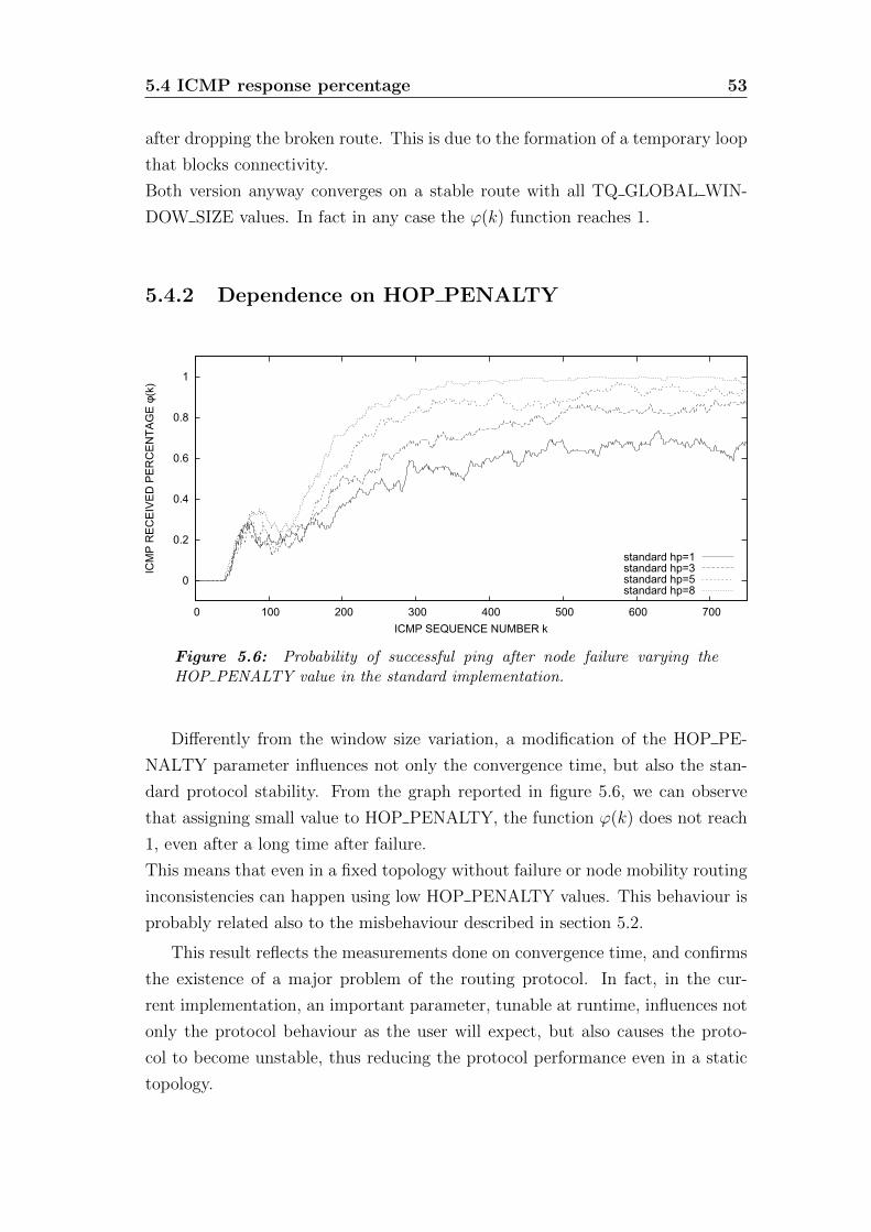
5.4 ICMP response percentage 53

after dropping the broken route. This is due to the formation of a temporary loop

that blocks connectivity.

Both version anyway converges on a stable route with all TQ GLOBAL WIN-

DOW SIZE values. In fact in any case the ϕ(k) function reaches 1.

5.4.2 Dependence on HOP PENALTY

0

0.2

0.4

0.6

0.8

1

0 100 200 300 400 500 600 700

ICM

P R

EC

EIV

ED

PE

RC

EN

TA

GE

φ(k

)


standard hp=1standard hp=3standard hp=5standard hp=8

Figure 5.6: Probability of successful ping after node failure varying theHOP PENALTY value in the standard implementation.

Differently from the window size variation, a modification of the HOP PE-

NALTY parameter influences not only the convergence time, but also the stan-

dard protocol stability. From the graph reported in figure 5.6, we can observe

that assigning small value to HOP PENALTY, the function ϕ(k) does not reach

1, even after a long time after failure.

This means that even in a fixed topology without failure or node mobility routing

inconsistencies can happen using low HOP PENALTY values. This behaviour is

probably related also to the misbehaviour described in section 5.2.

This result reflects the measurements done on convergence time, and confirms

the existence of a major problem of the routing protocol. In fact, in the cur-

rent implementation, an important parameter, tunable at runtime, influences not

only the protocol behaviour as the user will expect, but also causes the proto-

col to become unstable, thus reducing the protocol performance even in a static

topology.


5.5 Real test-bed

Figure 5.7: Test-bed used for node failure experiments. To simulate a sub-optimal path an HOP PENALTY factor of 100 has been set on node B2.

To validate the results obtained in the emulated network, we have built a real

test-bed using off-the-shelf devices. In order to compare results obtained in the

real world with the one obtained using emulators, we have built a topology very

similar to the one implemented in the emulation environment (see figure 5.1).

Clearly it is difficult to obtain exactly the same situation. This is true es-

pecially for link qualities, that in the emulator are fixed, while in the real word

are time varying. To overcome this problem, we have put the devices close one

another to obtain perfect local link. Then we simulated different link qualities

opportunely tuning the HOP PENALTY parameters of intermediate nodes. In

particular we setted an high HOP PENALTY value of 100 at node B2, that rep-

resent the back-off sub-optimal route. In this way, before failure of node B1, the

originator B2 is never chosen by C and D as router toward node A and vice-versa.

The real test-bed configuration is depicted in figure 5.7.

5.5.1 Standard B.A.T.M.A.N. convergence time

We have run the same experiment as in the emulated environment, using ICMP

packets to monitor connectivity between node A and stations C,D. We have also

used the same definition of convergence time, as defined in 5.2.

The obtained results reflect the emulation outcomes, confirming the slow

B.A.T.M.A.N. convergence after a failure due to a temporary loop formation.

Also the increase in convergence time variance using low HOP PENALTY val-

ues is confirmed. In particular average convergence time, resulting from the real

test-bed, are aligned with the average values obtained with the emulation. This

5.5 Real test-bed 55

0

10

20

30

40

50

60

70

80

1 2 3 4 5 6 7 8 9 10 11 12 13 14 15

CO

NV

ER

GE

NC

E T

IME

(s)

HOP_PENALTY

standardmodified

Figure 5.8: Average convergence time in case of node failure varying theHOP PENALTY measured in the real test-bed.

confirms that the simulation using virtual machines is a good technique to eval-

uate routing protocols behaviour.

The only difference observed is the absence of connection instability observed

in the emulated environment. This is probably due to the different network

topology, in fact the problem of local OGM echoes erroneously processed as path

OGMs, described in section 5.2, does not emerge because all existing direct links

are also optimal paths.

5.5.2 Modified version convergence time

As for the standard B.A.T.M.A.N. implementation, real world tests confirm the

results obtained in the emulated environment. Also the average convergence time

and variance are similar.

The results confirm that proposed modification guarantees loop-freeness and,

consequently, it assures bounded mean converge time 1. We confirmed that the

HOP PENALTY parameter tuning does not influence in any case the convergence

time, as the final user will expect. The convergence times measured in the real

test-bed are reported in figure 5.8.

1Convergence time will depend only from MAX SEQNO GAP, ORIG INTERVAL and OGMloss probability. It is not influenced by HOP PENALITY and by routing misbehaviour.


0

0.2

0.4

0.6

0.8

1

0 50 100 150 200 250

φ(k

)

ICMP SEQ. NUMBER k

modified g=3standard w=3

0

0.2

0.4

0.6

0.8

1

0 50 100 150 200 250 300 350 400 450 500

φ(k

)

ICMP SEQ. NUMBER k


0

0.2

0.4

0.6

0.8

1

0 100 200 300 400 500 600 700

φ(k

)

ICMP SEQ. NUMBER k


Figure 5.9: Comparison between standard implementation and mod-ified version with different values of TQ GLOBAL WINDOW SIZE orMAX SEQNO GAP. Can be noticed that standard B.A.T.M.A.N. convergesslowly due to a phase with non zero loss probability, caused by the formationof routing loops. The modified version, on the other hand, finds immediately anew stable route.

5.5 Real test-bed 57

0

0.2

0.4

0.6

0.8

1

0 50 100 150 200 250 300 350 400 450 500 550 600 650 700 750 800 850 900 950 1000

φ(k

)

ICMP SEQ. NUMBER k

modified hp=1standard hp=1

0

0.2

0.4

0.6

0.8

1

0 50 100 150 200 250 300 350 400 450 500 550 600 650 700 750 800 850 900 950 1000

φ(k

)

ICMP SEQ. NUMBER k


0

0.2

0.4

0.6

0.8

1

0 50 100 150 200 250 300 350 400 450 500 550 600 650 700 750 800 850 900 950 1000

φ(k

)

ICMP SEQ. NUMBER k


Figure 5.10: Comparison between standard implementation and modified ver-sion with values of HOP PENALTY less than the default value 10. Can benoticed that standard B.A.T.M.A.N. does not converges and remains in a situ-ation with non zero loss probability. Stability of modified version, on the otherhand, is not influenced by parameter setting.

Chapter 6

Conclusion

In the thesis we have tackled the problem of routing in Wireless Mesh Network.

We have focused our attention on the prominent B.A.T.M.A.N routing protocol,

describing in details its working principles and reporting also the various features

introduced in the latest versions.

We started providing a formalization of the Transmission Quality (TQ) rout-

ing metric employed in B.A.T.M.A.N., as till now a formal description was miss-

ing. Monotonicity and isotonicity of TQ metric have been demonstrated in an

ideal loss free situation, deriving a proof of optimality, consistency and loop-

freeness of the B.A.T.M.A.N. routing protocol in this ideal case.

Since B.A.T.M.A.N. routing information are sent in broadcast, we examined

whether losses of routing management frames, that can be frequent in wireless

networks, modify formal properties of the TQ metric. We evidenced that consis-

tency and optimality cannot be obtained without assuring guaranteed delivery of

routing management frames, so we concentrated our attention on loop freeness.

We have demonstrated that even a single OGM loss can cause TQ monotonicity

violation, possibly producing routing loops. We have built a sample scenario in

which monotonicity violation causes routing loops, and then we have identified

the factors causing this problem, which are path TQ averaging and a mechanism

that we called fast OGM forwarding.

The routing loops formation is a major problem for a routing protocol, so

a modification of OGM forwarding rules and path TQ calculation has been de-

scribed. The modification allowed the formal demonstration of the metric mono-

tonicity, deriving also a proof for loop freeness which is a fundamental character-

istic of a routing protocol.

To confirm our analysis, we have conducted a number of experiments in an

60 Conclusion

emulated, controlled scenario, where single node failures allow the repeatable

measure of the performance difference between the two protocol versions. We have

shown that the standard implementation convergence time is heavily influenced

by routing loops formation and depends also from TQ GLOBAL WINDOW -

SIZE and HOP PENALTY parameters. In particular when setting little value of

HOP PENALTY, the protocol exhibits intermittent connectivity that destroys

the performance.

On the other hand, we have confirmed that our modification is actually im-

mune from routing loops, and its convergence time is bounded. In particular

opportunely tuning MAX SEQNO GAP and ORIG INTERVAL we can balance

between a fast reactive protocol and a more stable one, depending on the network

characteristics. The results obtained in the emulated environment have been also

confirmed running the same experiment in a real test-bed.

In a future work, it would be interesting to test the behaviour of B.A.T.M.A.N.

in networks with mobile nodes. During this work we have collected sufficient clue

to say that, in a similar scenario, standard version can become unstable, causing

the formation of routing loops. The modified version, on the other hand, is

immune from loops so it would exhibit much better performance.

Appendix A

Mesh network emulation

For our emulation, we decided to use virtual machines running unmodified version

of the B.A.T.M.A.N. protocol. This approach has the advantage of not introduc-

ing errors coming from translation of the protocol into specific network simulators

such as NS-2.

As far as we know does not exist any network emulator capable to simulate

wireless links. So we decided to use a modification of the well known network

emulator VDE switch, to connect various protocol instances running on qemu

virtual machines. The wirefilter package has also been used to modify packet

loss probability and network delay. These tools are all parts of the VDE (Virtual

Distributed Ethernet) project 1.

This configuration works well for our objective of testing the convergence time

of the protocol, and in general it is suitable to analyse B.A.T.M.A.N. behaviour

in different network topologies and situations. On the other hand, a similar

approach cannot be used to estimate other protocol performance metrics, such as

throughput or delay. In fact, in the emulated test-bed all links are full duplex,

and there isn’t a simple way to simulate wireless links characteristics such as

bit-rate adaptation, retransmissions, inter and intra flow interferences, etc.

A.1 VDE

VDE (Virtual Distributed Ethernet) is a powerful tool that allow to create an

Ethernet compliant virtual network, that can connect different types of hosts. In

our case, we connect virtual machines all executed on the same hosts, and this

give us the possibility to create whatever topology we want.

1http://vde.sourceforge.net/

62 Mesh network emulation

QEMU

eth0

VDE switch

color 0

color 1

color 1

color 1

color 1

color 1

QEMU

eth0

VDE switch

color 0

color 1

VDE plug + wirefilter

Figure A.1: Illustration of VDE configuration. VDE switch only forwardsdata to ports with the same color thus allowing only direct neighbour commu-nication.

VDE offers tools to create the virtual counterpart of real network stuff, such

as switches and cables to interconnect the hosts. We will see that these tools

cannot be used directly in our case, but they need little adjustments to better

simulate a WMN.

A.1.1 VDE switch

VDE switch is the tool used to connect VDE hosts, or better VDE plug attached

to hosts. We cannot use directly VDE, because we do not want to create a unique

broadcast domain, but instead we want only neighbour nodes communicating

directly. In this way we enforce multi-hop communication, so B.A.T.M.A.N.

protocol can work properly.

The patch used to modify the standard VDE switch assign to each VDE switch

port a number (or color). The communication is allowed only if colors of ports

are different. In this way only one-hop neighbours can communicate directly. The

figure A.1 illustrates the concept.

A.1.2 VDE plug and wirefilter

A VDE plug is essentially a virtual cable used to connect different VDE switches.

To simulate network conditions such as packet loss, bandwidth or delay, the

wirefilter tool has been used. Wirefilter acts on packet traversing the virtual

cable, according to parameters provided independently from packet type.

A modification of wirefilter has been used to differentiate between different

packet type. In particular it is important to differentiate between broadcast

A.2 Qemu and OpenWrt 63

packets, that can get lost, and unicast packets that has substantially guaranteed

delivery, thanks to physical acknowledgements.

A.2 Qemu and OpenWrt

Qemu is an open source processor emulator that allow to emulate a number of

different system architectures. For our test we have used x86 machines running

an OpenWrt operating system. This choice is due the diffusion of this operating

systems in the world of access points and embedded devices, especially in low cost

network devices and in open community developing free wireless mesh network for

internet access 2. There already exist also commercial solutions for WMN based

on device running OpenWrt operating system, together with B.A.T.M.A.N. 3.

Interfaces of emulated machines are created using the vde back-end in order

to interconnect the machines using VDE switches as described above. For each

machine also a tap interface has been created to communicate directly with the

host machine, allowing to monitor and log the traffic on each machine network

interface.

A.3 B.A.T.M.A.N.

The B.A.T.M.A.N. module is natively available for OpenWrt. It can be chosen

between the development version and the latest stable version. For our tests we

used stable version 2011.3.1. The modified version has been also implemented

starting from this release source code.

The B.A.T.M.A.N. module has been added to Openwrt at compile time, but

can also be added at run-time using the ipkg utility.

2See for example http://start.freifunk.net/, http://villagetelco.org/ andhttp://wiki.ninux.org/

3http://www.open-mesh.com/

64 Mesh network emulation

Bibliography

[1] D. Furlan, R. Lo Cigno, “Analysis of B.A.T.M.A.N. routing protocol overhead

and TQ metric cross layer extension”, DISI Technical Report, DISI-12-005,

2012.

[2] I. Akyildiz, X. Wang, “Wireless Mesh Networks”, Wiley, 2009

[3] I. Chlamtac, M. Conti, J. Liu, “Mobile ad hoc networking: imperatives and

challenges”, Ad Hoc Networks, vol.1, pp. 13-64, July 2003.

[4] I. F. Akyildiz, W. Su, Y. Sankarasubramaniam, E. Cayirci, “Wireless sensor

networks: a survey”, Computer Networks, vol 38, pp. 393-422, March 2002.

[5] N. Nandiraju et al., “Wireless Mesh Networks: Current Challenges and Future

Directions of Web-in-the-sky”, IEEE Wireless Communications, vol. 14(4), pp.

79-89, Aug. 2007.

[6] M. Campista, P. Esposito, I. Moraes, L. H. Costa, O. C. Duarte, D. Passos,

C. V. de Albuquerque, D. C. Saade, and M. Rubinstein, “Routing Metrics

and Protocols for Wireless Mesh Networks”, IEEE Network, vol. 22, no. 1,

pp. 6–12, Jan.-Feb. 2008.

[7] C. Perkins, E. Belding-Royer, S. Das, “Ad hoc On-Demand Distance Vector

(AODV) Routing”, Proc. WMCSA ’99, pp. 90-100, 1999.

[8] DB Johnson, DA Maltz, Y-C Hu, “The dynamic source routing protocol for

mobile ad hoc networks (DSR)”, IETF Internet-Draft: work in progress, 2004

[9] T. Clausen, P. Jacquet, “Optimized Link State Routing Protocol (OLSR)”,

Proc. INMIC 2001, pp. 62-68, Aug. 2001.

[10] “Draft Standard for Information Technology - Telecommunications and In-

formation Exchange Between Systems - LAN/MAN Specific Requirements -

Part 11: Wireless Medium Access Control(MAC) and Physical Layer(PHY)

66 BIBLIOGRAPHY

specifications: Amendment 10: Mesh Networking”, IEEE unapproved draft,

IEEE P802.11s/D4.0, Dec. 2009

[11] K. N. Ramachandran et al., “On the Design and Implementation of Infras-

tructure Mesh Networks”, IEEE Workshop in Wireless Mesh Networks, Sept.

2005

[12] D. Passos et al., “Mesh Network Performance Measurements”, 5th Inter-

national Information and Telecommunicatios Technologies Symposium, Dec.

2006.

[13] D.S.J. De Couto, D. Aguayo, J. Bicket, R. Morris, “A high-throughput path

metric for multi-hop wireless routing”, ACM MOBICOM ’03, pp. 134-146,

Sept. 2003.

[14] R. Draves, J. Padhye, B. Zill, “Routing in multi-radio, multi-hop wireless

mesh networks”, ACM MOBICOM ’04, pp. 114-128, 2004.

[15] L. Iannone, S. Fdida, “Mrs: A simple cross-layer heuristic to improve

throughput capacity in wireless mesh networks”, In proceedings of CoNEXT

2005, Oct. 2005.

[16] L. Iannone, K. Kabassanov, S. Fdida, “The real Gain of Cross-Layer Routing

in Wireless Mesh Networks”, In Proceedings of Second International Workshop

on Multihop Ad hoc Networks: from Theory to Reality, ACM/SIGMOBILE

RealMan ’06, 2006.

[17] A. P. Subramanian, M. M. Buddhikot, S. C. Miller, “Interference Aware

Routing in Multi-Radio Wireless Mesh Networks”, IEEE Workshop Wireless

Mesh Networks, pp. 55–63, Sept. 2006.

[18] Y. Yang, J. Wang, R. Kravets, “Designing routing metrics for mesh net-

works”, In WiMesh, 2005.

[19] T. Liu, W. Liao,“Capacity-aware routing in multi-channel multi-rate wireless

mesh networks”, In Proc. IEEE International Conference on Communications

(ICC), pp. 1971–1976, 2006

[20] R. Draves, J. Padhye, B. Zill, “Comparisons of routing metrics for static

multi-hop wireless Networks”, In Proc. ACM Annual Conference of the Special

Interest Group on Data Communication (SIGCOMM), pp. 133–144, 2004.

BIBLIOGRAPHY 67

[21] A. Neumann, C. Aichele, M. Lindner, S. Wunderlich, “Better approach to

mobile ad-hoc networking (b.a.t.m.a.n.)”, IETF Internet-Draft (expired Octo-

ber 2008), Online Available:http://www.open-mesh.net/, April 2008.

[22] Abolhasan M., Hagelstein B., Wang J.C.-P., “Real-world performance of cur-

rent proactive multi-hop mesh protocols”, APCC 2009, pp. 44-47, 2009.

[23] C. Perkins, P. Bhagwat, “Highly-dynamic destination-sequenced distance-

vector routing (DSDV) for mobile computers”, Proc. SIGCOMM ’94, pp. 234-

244, Sept. 1994

[24] A. Quartulli, R. Lo Cigno, “Client announcement and Fast roaming in a

Layer-2 mesh network”, DISI Technical Report, DISI-11-472, 2011.

[25] Y. Yang, J. Wang, “Design Guidelines for Routing Metrics in Multihop Wire-

less Networks”, In Proc. IEEE INFOCOM ’08, pp. 1615-1623, 2008.

[26] R. G. Garroppo, S. Giordano, L. Tavanti, “Experimental evaluation of two

open source solutions for wireless mesh routing at layer two”, 5th IEEE Inter-

national Symposium on Wireless Pervasive Computing (ISWPC), pp. 232-237,

May 2010

elaborato finale - open-mesh · 2012-03-03 · elaborato finale improving b.a.t.m.a.n. routing...

Documents