electricity transmission pricing: the new approach

Electricity transmission pricing

The new approach

Sally Hunt and Graham Shuttleworth

Competition in electricity markets has led to the recognition that electricity needs to be priced on the basis of marginal costs which vary by time of use. Increased access to transmission networks has led to an expansion of this view, beyond time of use, to the place cf use. This paper examines a new approach to transmission pricing derived from the fundamental principles of transport economics. It shows how pricing based on short- run marginal costs can be reconciled with appropriate signals for long-term investment and monopoly in an integrated transmission system.

Keywords: Transmission pricing; Electricity; Transport econo-

mics

Transmission pricing in electricity is undergoing a conceptual revolution. It is now widely accepted, on both sides of the Atlantic, that marginal costs’ are the appropriate basis for pricing both regulated and competitive generation, and that they vary by time of use. The new transmission pricing involves expanding our view beyond time of use, to place of use. The advent of competitive markets is focusing atten- tion on locational aspects of pricing, and the debate is now drawing on familiar concepts, such as opportunity costs and the marginal cost of transfers between nodes of a network system.

At the same time, advanced computing power makes it possible to model line flows on networks, so that the costs of individual transactions can be assessed. What is needed is a conceptual framework in which the alternatives for pricing can be discussed. One such framework was proposed in the early

Sally Hunt is a director senior consultant with Associates (NERA), 15 9AF, UK.

98

and Graham Shuttleworth is a National Economic Research Stratford Place. London WlN

1980s by a group at the Massachusetts Institute of Technology (MIT) in their work on spot pricing’ and the short-run marginal costs of electricity.3 Their basic insights underlie most contemporary discussions of transmission pricing.

However, as we show in the next section of this paper, the concepts now being applied to electricity are the same as the basic theorems of transport economics: the MIT group only added the computational methods for applying them to electricity. Electricity presents some complex operational and computational problems, but most of the conceptual problems have counterparts in the transport problems of other product markets.

The new approach looks first at short-run costs. This does not depend on setting up a spot market in transmission: contracts can always be written in different ways, to reduce risk and to cut transactions costs. One model to follow is the new electricity market in England and Wales, where a day-ahead power pool coexists with long-term contracts.

The fundamental insight of the new transmission economics is: that the cost of transport between two nodes is equal at any time to the difference between the market prices of the product at those two nodes. The economics of transport is therefore closely tied up with the markets in the product being transported; market prices in different locations both drive and are driven by the transport costs between them. The aim of this paper is:

0 to develop this fundamental idea in the context of transportation in general;

0 to identify short-run marginal costs in the specific context of electricity transmission;

0 to consider the regulatory problems when transmission is provided by a monopoly car- rier; and

0 to suggest contractual mechanisms which might meet the requirements of efficiency and revenue recovery.

0957-l 787/93/020098-l 4 0 1993 Butterworth-Heinemann l_td


manufactured products. But it did not benefit two groups of people: those who had previously sold coal to Manchester from elsewhere at high prices, and those who had consumed low-price coal close to the coal field.

0 The gains from trade go to the exporting producer and the importing consumers; pro- ducers in the importing area, and the consumers in the exporting area, are the losers.

This is a universal effect of trade. The impact on the losers is much discussed in economic theory and is also the genesis of real policies, like protective tariffs, opposition to free trade, and objections to open access on transmission wires. At the heart of many discussions which appear to be about transmission pricing, there are really concealed questions about the resulting trading opportunities: who is going to sell what to whom? We shall not develop this point further in this paper, but it is worth remembering.

The effect of competition

The price of transport affects the deployment of resources and the location of industry. As in every other market, those who provide a service will charge what the market will bear: the Duke of Bridgewater held a monopoly for some time and no doubt kept his price above the competitive market price. But if there is competition, then the following essential features of a competitive market hold.

0 The price will be driven to the short-run marginal cost, including the value of constraints; the value of constraints is also called the ration-

ing price (what customers are willing to pay). 0 New entrants will enter if the price is higher

than the long-run marginal cost of providing the service. This provides a long-run upper limit to the price.

In an equilibrium situation, one would expect the following rule to hold once the various price movements have been worked out by competition:

The price difference between two locations = The short-term marginal transport cost

between the same two locations = The long-run marginal transport cost

between the same two locations

Transport as a paradigm

Coals to Manchester

The basic similarity of transport and transmission can be seen in an early instance of energy economics: the movement of coal from Lancashire mines to the industrial centre of Manchester. Initially, the coal was carried by horse and cart, at great expense. The difference in the price of coal between the pithead and Manchester was due to the transport charge. Neither the mines nor the city could have developed on this basis; the cost of transporting coal into the city rendered it uneconomic as an industrial energy source. The price paid to miners would have been too low to support much mining activity, and the price charged to factories would have been too high to allow competitive production.

With the advent of the Duke of Bridgewater’s canal in the eighteenth century, the situation changed dramatically. The Duke could charge less than the horse and cart, reducing the delivered cost in Manchester, and could rely on the consequent expansion of demand for coal to fill up the barges on his canal. As the demand expanded, it was possible to pay miners a price sufficient to encourage de- velopment of more expensive mines, while maintaining a relatively low coal price to city dwellers. Both the mines and Manchester began to grow.

Growth and competition were accelerated greatly by the advent of the railways in the nineteenth century. The reduction in transport costs allowed an even higher price to be paid to mines (and for mining to exploit yet more costly seams), while maintaining or lowering the price of coal in Manchester, thus allowing the city to develop into the fine industrial metropolis we know and love today.4

This historical process illustrates two facets of the interrelation of product and transport prices. The first is the realization that transportation pricing is not separable from conditions in the market of the product being transported:

@ Demand for transport is derived from supply and demand in product markets.

The second point describes the final relationship between transportation and product prices:

0 For any product, the price difference between two markets is set by the cost of transport between them.

The gains from trade

Reducing the price of transport benefited the Lan- cashire coal miners, the manufacturers in Manches- ter, and probably the customers who bought the

The value of constraints

Short-run marginal costs include the value of the constraints. When supply is limited, the price rises automatically to the (marginal) value of the service in a competitive market. There are two ways to say

UTILITIES POLICY April 1993 99


this: either you say, ‘in a competitive market, price equals the short-run cost, which includes the cost of constraints,’ or you say ‘price equals short-run cost, unless there is a constraint, in which case price rises to the value of the products.’ Some people find this confusing, as it seems to mix pricing on the basis of costs with pricing on the basis of value. In what sense is this value of the constraint a ‘real’ marginal cost?

Again, look at a transport example. The plane to New York is full, and I have to wait for the next one; this costs me 4 hours of my time, which is the real cost of the constraint. The airline might be asked to pay me for my discomfort. (This is a feature being introduced in various regulated services.) Instead, the airline could ask for volunteers to get off the plane. Someone might be willing to do it in return for less than the cost of compensating me for the waste of my time; the airline could then deal with the constraint at lower cost. If the airline puts on another plane, it can also avoid paying me, but this would probably cost more than the cost of the constraint. Constraints therefore impose real costs: the value to consumers (what the marginal customer is willing to pay) gives one estimate of the opportunity cost, and there may be other ways of spending money to meet the constraint.

Another common preconception or confusion is that constraints are ‘bad’ things that ‘should’ be removed: if the cost of removing the constraint exceeds the value of removing it, then it should stay. Indeed, as we show below, efficient investment will normally leave constraints in every market. As we showed in the airline example, optimizing the system (by asking for volunteers with a lower value to their time) means that the cost of constraints is minimized.

Even so, it is usually not worth while to invest to meet every conceivable demand for a service: for example, by having a second aeroplane available. Whenever it costs something to eliminate a constraint, there will be some occasions when it is better to charge a rationing price. In a highly capital- intensive industry, this is the only feature which will enable short-run marginal cost pricing to earn sufficient revenues to cover the costs of investment.

Losses of the product

The cost of transportation includes the losses of the product in shipment. Sometimes these are simply deterioration, as in food markets, and sometimes the product is itself used up during transport, as for example with coal on the steam railways. The difference in the prices in the two markets will include these product losses. There are two points to note

about losses. First, the contract between the transporter and the

producer may or may not include payment for losses: this is a matter of who takes the risk in shipping. But the cost of transport, and the difference in price between the markets, always includes the value of the losses.

To show this, with a change of metaphor, consider bananas. If half the shipment is lost to bruising, this is part of the cost of shipment. A better ship or crew, which bruised less but charged more, could have the same total cost to the producer. Or the shippers might internalize the losses, charging more for the transport and buying in bananas to cover the losses, but making their own decisions as to whether to take more care with handling.

This analogy applies directly to electricity transmission, where the cost of losses is part of the marginal cost of transmission, whoever bears them in the contract. But the banana example also permits us to see the difficulty of computing the value of the marginal losses: if the physical losses are 2073, then the shipper buys 25% more bananas than he expects to deliver. Suppose the price in the Caribbean is f2, while in London it is &6. Some of this difference can be accounted for by the costs of ship, fuel and crew, but what is the value of the losses? In the Caribbean the extra cost of the lost bananas was f2, but in London it was f6. The lost product increased in value as it was shipped, along with the unbruised product.

Second, if the percentage losses increase with the load transported, it can be shown that marginal losses, and not average losses, are the relevant item in determining the marginal cost of transport. If a lightly loaded ship would only lose 15% of the bananas, and the more it is loaded, the higher the percentage it loses, then the price differences between ports will be determined by the marginal

losses of the last boat pulled into service, or the incremental losses due to the last load put on board.

Products change in value depending on their location

The examples in the previous sections have shown that the ‘same’ product can have different values, depending on location. Strictly, it is more useful to think of the price in any transaction, or in a simul- taneous set of transactions called a market, as being defined by product, time and place. Prices of the same product at different places differ by the transport costs, or arbitrage will take place to remedy the difference. On a linear transportation system (a single transmission line, a road or rail link), the prices will increase monotonically in the direction of

UTILITIES POLICY April 1993

Electricity trunsmission pricing

never differ between two separate locations by more than the short-run marginal cost of transporting the product from one location to the other, including the cost of constraints. In the electricity sector, a cost- minimizing despatcher will attempt to equalize marginal generation costs throughout the system, subject to costs of transmission. In this sense, the despatcher is performing the function normally per- formed by separate traders in competitive markets.

The elements of transmission taken into account by the despatcher include: (a) transmission losses; and (b) constraints.

net flow, and the price difference between any pair of places will equal the transport costs between them. On a network system, the equilibrium set of prices at the nodes will all be differentiated from the other nodes by the transport costs between them.

Negutive transport costs

It is worth mentioning that transport costs can be negative. Suppose that, for some reason, someone in Manchester wished to sell coal to someone at the coalfield. He might buy a load of coal at the high Manchester price and physically transport it. Or, if he had any sense, he would send word to the coalfield not to transport a shipment, and divert it to the customer at the coalfield. This is analytically equivalent to buying in Manchester and incurring negative transport costs.

In electricity transmission it is even easier to see the negative costs, because additional net flows against the main flow do indeed reduce losses on the system, may reduce constraints, and do actually save real resources.

Implications for the rest of this paper

Since our task in this paper is to investigate appropriate prices for regulated transmission of electricity, let us immediately state that we see the task as being to ensure economic efficiency by emulating the results of a competitive market, and to ensure that the incentives at each location are, as far as possible:

0 to set the price of transport equal to short-run marginal cost, including the cost of constraints, to achieve minimum total cost on the existing system;

0 to ensure that the incentives for investment are such that when the short-run marginal cost (SRMC) exceeds the long-run marginal cost (LRMC), investment takes place;

and in addition, to ensure the financial viability of the transmission company by ensuring that:

0 the revenues are sufficient to cover the costs of the company.

A competitive market with no economies of scale would achieve these objectives, but in a regulated monopoly there will usually be conflicts between the objectives. Before turning to the tariff structures themselves, the next three sections examine the relationship of SRMC, LRMC and revenue requirements on an electricity transmission system.

Short-run costs of transmitting electricity

In a competitive market, the price of a product can

Transmission losses

An unconstrained zone is one within which there are no transmission constraints. Within any unconstrained zone, the only marginal cost of transmission is given by the physical losses.

At any node Z in the unconstrained zone, the marginal value of electricity will equal the cost of generating additional supplies at any other node Y, and transmitting it from Y to Z. If extra energy is sent into the zone at point Y and extra demand is placed on the zone at point Z, there will be a net increase in line flow between Y and Z. This line flow will have a measurable effect on total losses. Any increase or decrease in total losses, on the network as a whole, is then the marginal loss associated with transmission from Y to Z.

If the marginal loss is positive, this means that less can be drawn off from Z than is supplied at Y, the difference having been lost on the network. For example, any generator supplying an additional 100 MWh at Y may find that the customer at Z can only draw off an additional 95 MWh. Marginal losses are 5 MWh (or 5% of generation). These are the physical losses. What is the cost of the transmission?

If the marginal cost of generation at Y is flO/ MWh, the total cost of the additional output of 100 MWh is f1000. However, the customer is only able to receive an extra 95 MWh, for which he must also pay the generator EIOOO, or f10.53/MWh. In other words, moving energy from Y to Z raises the price by 53p/MWh. The transmission cost from Y to Z is therefore 53pfMWh.

Generally speaking, losses increase with distance, so that the farther apart the nodes are, the higher the electricity price must rise to cover the generator’s cost of supply. However, additional line flow only raises total losses if it moves in the same direction as the existing net flow.

If the flow is from Z to Y, ie aguinst the current net flow, total losses on the system will be reduced; the marginal losses of such a transaction would be



negative. In such cases, a generator might get away with supplying 95 MWh at Z to meet additional demand of 100 MWh at Y; the marginal effect on losses is to save 5 MWh. In this case, if the cost of

generation at Z were flOS3/MWh, or &lOOO in total, the generator would only need to charge flO.OO/ MWh at Y for the 100 MWh delivered. In other words, the effect of moving electricity from Z to Y, against the current net flow, would be to save transmission losses and to reduce the price by 53pl MWh. The transmission cost from Z to Y would then be negative.

Constraints

If the security conditions limit the permissible flow on any line, some plants, which would be called to generate on the strength of their impact on generation costs and losses, are replaced by others which are more advantageously located.

On an electricity transmission system, the constraints are of two main types: thermal limits and regional voltage stability limits. Whatever the cause, they usually cause the despatcher to restrict max- imum flow over a line, thus driving a wedge between the marginal costs at either end of the line, so that the difference exceeds the marginal line losses. It is as if a constraint were a super-large transmission loss.

Imagine a grid system which can be divided into two zones, A and B. (We are ignoring marginal losses in this example.) Suppose initially that the level of demand is such as to suggest that the despatcher call up generation in both zones with a marginal cost of generation of fl6/MWh, but that this requires a substantial flow from generators in zone A towards demand in zone B, and that this flow is not limited by constraints on the transmission system.

Now impose a constraint on the amount that can flow over lines linking zone A to zone B, such that generation must be pulled back in zone A and replaced with generation in zone B. The resulting change in the pattern of despatch might, for instance, reduce the marginal cost of generation in zone A to fl4/MWh, whilst simultaneously raising it in zone B to flS/MWh. The price charged for transmitting energy across the link from A to B should then be f4/MWh, ie the difference in energy prices between the zones.

The f4 cost of the constraint may be understood in three ways, as follows.

tional generation costs of f4. This might occur, for instance, if another grid system connected to zone A was to try to wheel energy to a third grid system connected to zone B. The only way in which the local despatcher could accommo- date the additional input into zone A would be to back off on local generation, thereby saving &14/MWh; however, any additional demand out of zone B would have to come from local generation costing f18/MWh. Even before accounting for transmission losses, therefore, accommodating the demand for wheeling over the constraint raises generation costs by the net figure of f4lMWh.

0 The value oftransmission. The right to transmit over the constraint is a right of way, with a value like any other. In this case, any generator or customer who has the right to use the link is able to buy energy in zone A at the marginal price of fl4/MWh and to sell it in zone B at the marginal price of flS/MWh, making a profit of f4lMWh on the deal. Any other seller who wishes to buy a transmission right over the constraint will therefore have to pay the existing users at least this much for it, to compensate them for the profit forgone. The profit forgone by existing owners of an asset (in this case, a transmission right) is usually referred to as the opportunity cost; it is determined by the user who is prepared to place the highest value on the asset and to outbid all others for the use of it.

l Long-run marginal cost. The final sense in which the transmission price of f4/MWh might be said to bear some relation to costs is in regard to the costs of reinforcing the link. If some users are apparently prepared to pay f4/MWh to transmit energy from A to B, one should at least ask the question whether it would be worth building additional capacity, if it could be sold for this price. Should a constraint be allowed to persist, it would be possible to infer (though only in a fully competitive transmission sector) that the cost of reinforcing the link lay above f4/MWh.

The last comparison points to a relation between the short-run marginal costs of transmission and the incentives to invest. This link will be examined in detail below in the section on ‘Investment decisions and LRMC’.

0 Generation costs. In the example in the pre- SRMC as the difference between two energy spot

vious paragraph, incremental demand for prices

transmission across the constraint causes addi- The SRMC of transmission can (only) be derived

102 UTILITIES POLICY April 1993


A 6

Figure 1. Transmission loss factors (equal loss rate contours): typical winter night.

from the difference in energy spot prices between the two nodes in an optimized despatch. Suppose the pattern of constraints is used to divide the country into zones, within which electricity can move without constraint.

0 Within a zone, the difference in price between two nodes is derived from the marginal physical losses.

0 Moving from one zone to another, the marginal cost is the value of the constraints between them.

This assertation is based on the assumption that the despatcher really has minimized the total cost of generation and transmission. The cost of transmission losses and constraints cannot be calculated and minimized separately from the costs of generation. Since the value of losses and constraints is derived from and determines the pattern of generation, the whole system is optimized by minimizing the cost of

generution subject to the construints on the system, and recognizing the quantity losses between nodes.

If increasing generation at node B and reducing it at node A reduces total generation costs, then the despatcher, or the computer program, should do this, and the resulting pattern of generation marginal costs is spatially differentiated by the marginal losses

plus the constraints. This is the only way that we can unambigously state the marginal costs of transport. (See the earlier banana example.) Then, the difference in generation costs within an unconstrained zone is due to losses, while the difference between the nodes lying on either side of a constraint gives the value of the constraint.

The industry’s long-standing knowledge of physical transmission conditions can be combined with the recent expansion in computing power to compute these costs more efficiently than ever before.

Short-run marginal costs in England and Wales

Losses and transmission loss factors

Figure 1 shows a map of the marginal transmission losses across England and Wales, estimated for typical night-time operation on a weekday in the winter months. It is derived from a computer model which calculates the effect of injecting an additional 100 MW of power at any node, and increasing demand proportionally at each consuming node. The map shows a series of contours, ranging from +6 near the Scottish border to -4 in the South West. These figures are percentage physical marginal losses, known as transmission loss factors (TLFs), and the contours link points with equal TLFs. The TLF for consumption at each point is equal and opposite to the TLF for generation at that point.

There are two ways to understand the TLFs: they are used to optimize the despatch, and once the despatch is optimized, they give the contours of the difference in cost, taken from some arbitrary point.

Location of the ‘market’ is irrelevunt to desputch

First consider the despatch: the despatcher should aim to equalize the marginal costs of power delivered to any arbitrary point. The effect of transporting power, for example, from the Scottish border to the South West, is that part of an incremental MW of power will be ‘lost’ on the way (10% according to Figure 1). If a plant in the South West is available at a cost of f2.20/MWh, while a plant on the Scottish border is available at f2.00, the plant in the South West is more economic, because the real cost of transit from the border is about 10% of the generation (actually 6% for delivery to the centre of the country and 4% of the remainder for delivery to the South West, making 9.6% in total). Only 90.4% will reach the South West. The real cost delivered to the South West is f(2/0,904)/MWh = f2.2UMWh. So plants in the South West should be despatched up to the cost per MWh of 52.21, while those on the



Table 1. Energy equivalences.

Quantity Price Revenue

Sent out at TLFY contour 100 1 100

Delivered at 0 TLF contour 100 x (lbTLFY%) 1 100

(l-TLFY%)

Delivered at TLFZ contour 100 x (l-TLFY%) (1 -TLFZ”/o) 100

(1 -TLFZ%) (l-TLFY%)

border should only be despatched up to a cost of f2.00.

Constraints

Of course, plants on the border are not generating in order to deliver specifically to the South West. We can name any arbitrary point as the ‘location of the market’ and show that the same arithmetic holds. In England and Wales, the zero TLF line is a conve- nient point, because it runs through the centre of the country, and has the useful property of staying in much the same place for many patterns of generation. Then, the cost of delivering a unit of power from the border raises its price by 6%) while the cost of delivering the power from the South West reduces its price by 4%:

To extend the same analysis to constraints, we have found it useful to show a constraint as the place where the contours on the loss map fall very close together, in fact on top of each other, like a cliff on a relief map.

0 the equivalent price of MWh costing &2 at the border, if delivered to the market at the zero loss line, is f2.13 (=f2.04/0.94);

Figure 2 shows a transmission constraint across the country, which increases the difference in value between the two regions. Here, the TLF contours have been converted into price contours, assuming a market price of fl4/MWh in the middle of the northern zone (at the 4% TLF line) and fl8/MWh in the middle of the southern zone (at the zero TLF line). The difference between these two market prices is therefore f4iMWh.

a a plant in the South West, delivering to the market at 52.13 can afford to generate at 52.21 (= f2.13 x 1.04).

The despatcher must take the losses into account in deciding the order of despatch, but it is irrelevant where he considers ‘the market’ to be, or who is responsible for delivery.

The price contours continue on either side of the constraint, but are separated by the cost of the constraint, in this case f3.5OIMWh (= f17.64-E14.14). The remaining price difference between the northern and southern market prices (fO.SO/MWh) is accounted for by the cost of losses incurred in getting to and from the constraint.

Price Rule

The value of electricity at the market is therefore the same for power delivered from every node. But the value at any node differs by location, by the marginal cost of the losses between the nodes. Table 1 shows the arithmetical rules of equivalence between different locations.

The same analysis applied to demand suggests that a consumer on the border incurs negative marginal costs in bringing the power from the market; in fact, his consumption of 100 MWh reduces losses on the system by 6 MWh. A consumer in the South West requires 104 MWh to be generated for each 100 MWh he uses. Where a customer buys energy from a generator located right next door, he obviously incurs no additional losses; this can be accounted for by offsetting the losses incurred in delivering the generator’s output to market against the equal and opposite losses in delivering from the market to the customer.

Figure 2. Nodal electricity prices (equal price contours): typical winter night.



year contract takes some risk out of the system, and the appropriate price would be the three-year marginal cost. The appropriate price would be the expected short-run marginal cost, or E(SRMC), which one would expect to reflect the long-run cost of marginal additions to the grid. And as we now show, these costs are related to each other. In fact, with perfect foresight, the short-run marginal cost (including the cost of constraints) would equal the long-run marginal cost of constructing a new line and transmitting energy along it.

The same analysis applies as in the earlier example of losses: if getting the power to the market involves crossing the constraint, then the value of the power in the export-constrained zone is lower than the value in the other zone by the cost of the constraint; the cost of getting it to market from any location is the short-run marginal cost (TLF plus constraint). The cost of getting it back again to the customer in the constrained zone is negative.

Investment decisions and LRMC

The LRMC and the SRMC Why build? Criteria for construction and expansion

Discussions of marginal cost pricing often get very muddled by the so-called conflict between short-run and long-run marginal costs. This is sometimes because of the intuitive notion that SMRC is very low, but construction (and hence LRMC) is expensive. However, as we have shown, SRMC includes the cost of constraints and, except in a very overbuilt system, this is a large part of the SRMC.

Marginal costs are all costs present and future (but not past) of providing an increment of a service or product. So the relevant question is the marginal cost of what, given what? At any particular time, some costs are fixed for a certain period ahead, and others are variable. The longer the period ahead, the more costs are variable, since plant can be built, labour contracts renegotiated, and so on.

Short-run marginal costs are the variable costs of production of a small increment taken now, given that almost all factors of production are fixed: or, if capacity is limited, the price necessary to ration demand to capacity.

The marginal cost of increasing output at some time in the future (say, three years hence) may be lower, because something could be done to change the other factors of production. The cost of an increase in output using current capacity might be very high but, if new plant were added, it could be reduced. The marginal cost of output in three years’ time would be determined by the minimum cost method of increasing output, after allowing for any feasible adjustments to production methods.

The calculation of long-run marginal costs allows all factors of production to be fully variable, and sometimes even assumes a system fully adjusted to a long-term increment.

At any point in time, the short-run marginal cost can be shown to be the price which would make best use of the existing resources and for that reason economists, who preach economic efficiency, prefer it for pricing. But this does not mean that all transactions have to be spot transactions; a three-

The analysis above focused on the SRMC of transport or transmission, assuming that a link of a given size was in place between two nodes. However, there is a cost involved in providing any link in the first place. This raises the following questions.

0 What are the criteria for deciding whether to build or to expand a transport or transmission link between two places?

0 How large should the link be? 0 What is the relation between the SRMC

observed on the resulting link and the cost of putting the link in place in the first place?

Take two non-connected systems A and B, with supply (marginal generation cost) curves S(A) and S(B). They are generating, or planning to generate, to levels X and Y. Is it worth building a link between them?

How much to build is determined by the following rule:

0 Build until the marginal savings equal the marginal costs.

However, the decision on the quantity to build depends upon whether the project as a whole is beneficial. The criterion for building at all is given by the following rule:

0 The total savings in generation costs must exceed the total cost of transmission, including construction and losses.

These rules are examined further below.

Marginal cost equals marginal savings

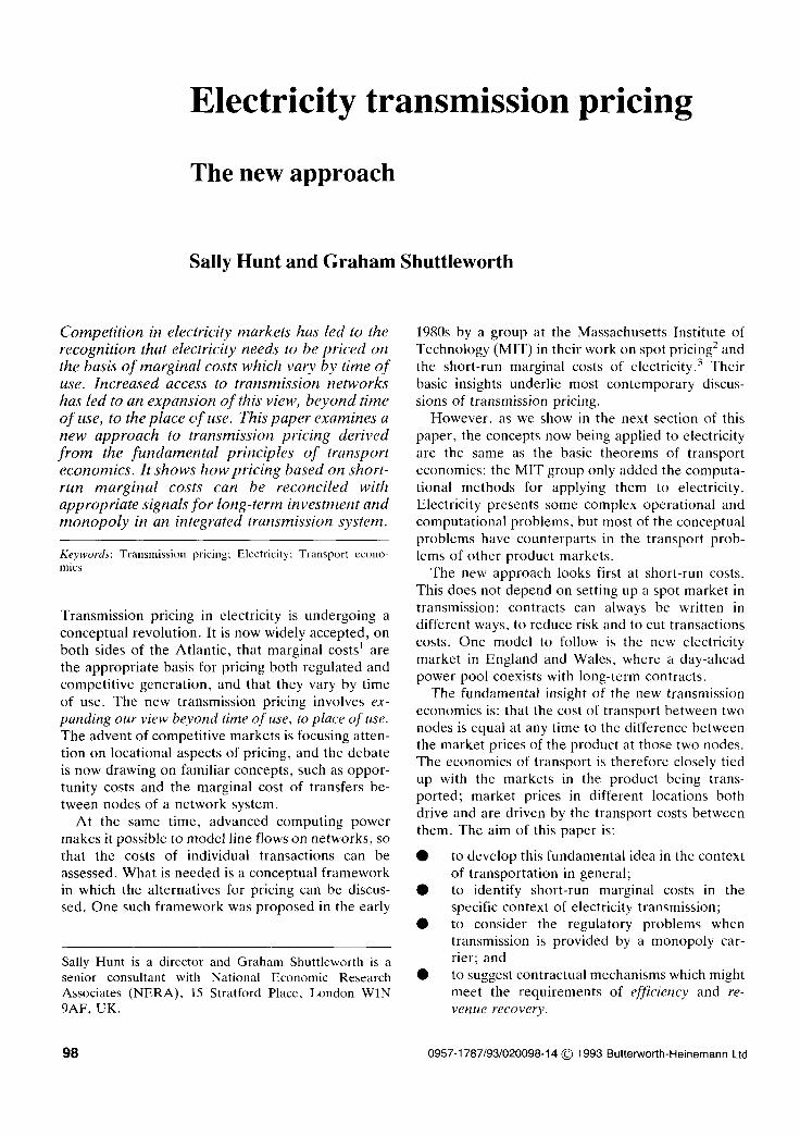
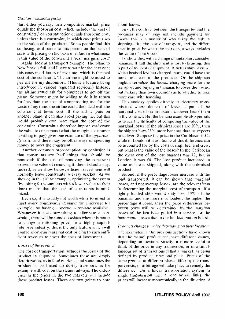
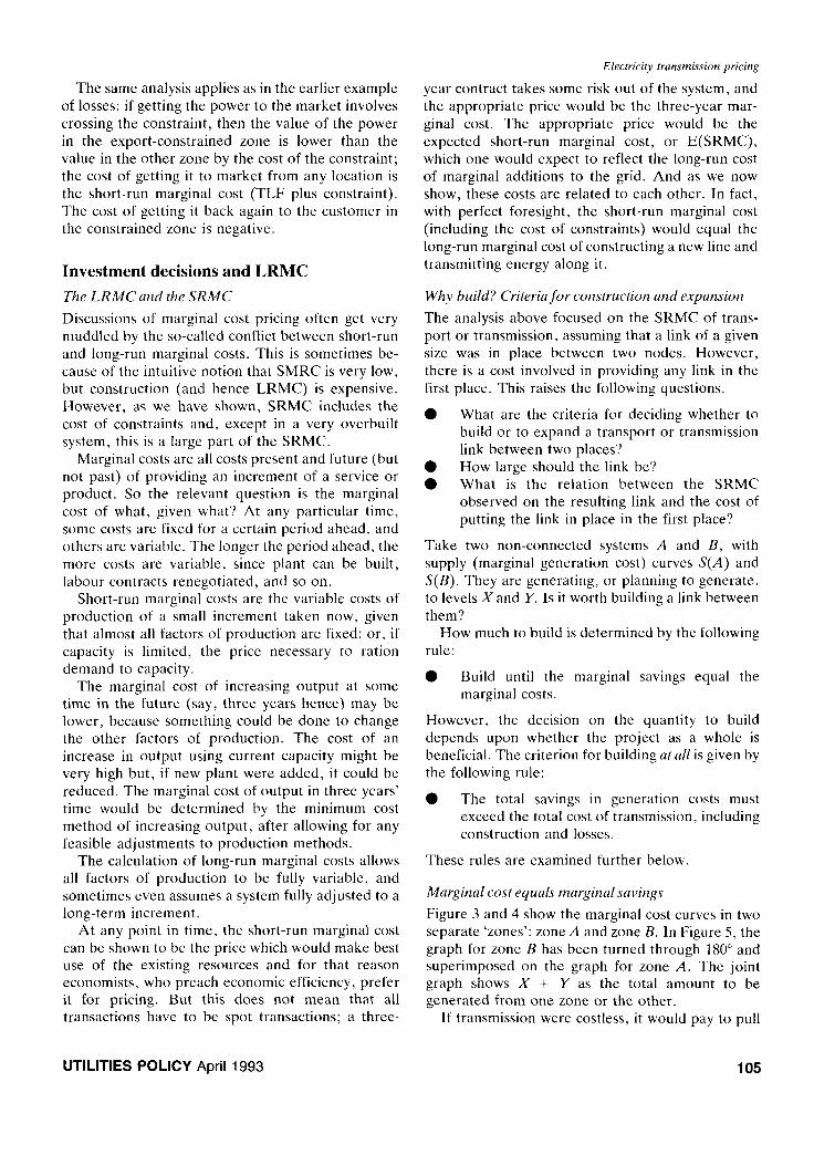
Figure 3 and 4 show the marginal cost curves in two separate ‘zones’: zone A and zone B. In Figure 5, the graph for zone B has been turned through 180” and superimposed on the graph for zone A. The joint graph shows X + Y as the total amount to be generated from one zone or the other.

If transmission were costless, it would pay to pull



flMWh Demand f/MWh f/MWh

31 Zone A -

IX MW

Figure 3. Zone A generation

back on the output from B and expand the output from A until the marginal costs at each place were equal. But since transmission is not costless, the rule is to build until:

Marginal costs of new line = the difference in the supply curves

Any more transmission would cost more than it would save; any less would forgo opportunities to make transactions economically. The relevant costs are construction costs plus losses on the actual transactions, ie the long-run marginal costs (LRMC).

Once this is done, and the construction has taken place, if the world turned out as planned, the SRMC on the resulting system is given by the difference between the supply curves (spot prices) at the point of equilibrium. Since we did not build enough to meet all conceivably economic transactions, but only those that were justified by the cost of the line, there will be constraints on the system, which will ensure that there is a wedge between the spot prices in the two zones sufficiently often to earn a return which

f/MWh Demand

I_

i !one B - I Y

MW

MW ’ Zone A + +Lone I MW

Figure 5. Joint generation.

covers the LRMC for each unit of transmission capacity built.

If things work out as planned, SRMC = LRMC

There is no mystery as to why the SRMC should equal the LRMC; the SRMC is defined as the marginal cost of transmitting, with capacity fixed. The LRMC is defined as the marginal cost of transmitting if capacity is variable. If it is cheaper to adjust capacity, that should be done; capacity should be added until the expected value of the SRMC has

been reduced to the LRMC. It follows that LRMC pricing should give the same

revenues as SRMC if the world turns out as the

planners expected. If the world does not turn out as expected, then

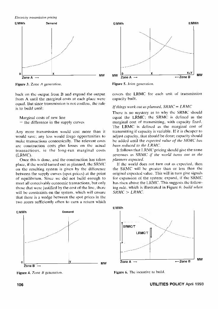
the SRMC will be greater than or less than the original expected value. This will in turn give signals for expansion of the system: expand, if the SRMC has risen above the LRMC. This suggests the following rule, which is illustrated in Figure 6: build when

SRMC > LRMC.

f/MWh

\ SRMC/T

:one A -t + Zone B MW

Figure 4. Zone B generation. Figure 6. The incentive to build.



costs of the line. This situation obviously raises

serious problems for charging mechanisms based on SRMC, despite the supposed efficiency merits of such a ‘competitive’ outcome.

f/MWh Price of Constraint

covers total costs

‘one A -+ +Zone B MW

Figure 7. SRMC covers costs: price of constraint covers total costs.

As we have seen, in a perfectly predictable world, there would be no difference between SRMC revenues and LRMC revenues; and if there were no economies of scale, both would cover the revenue requirement. But in the real world, the revenues from marginal cost pricing may not equal the required revenues. There is an extensive literature on this subject, which we summarize briefly.

Criterion for building anything at all

There is no point in building anything at all if the total savings from building do not exceed the total costs. Each of the vertical arrows in Figure 7 represents one unit of transmission capacity; the vertical height of the arrow represents the long-run marginal cost of the unit concerned. The arrows are all the same length; ie, the cost of every additional unit of transmission is the same, and there are no scale economies. The total savings of the first units trans- mitted are much greater than the cost of the transmission link: every succeeding unit saves less, until the last unit saves just as much as it costs. In this diagram, there are two things to observe: it is certainly worth building, and pricing at marginal cost will recover the required revenues (since LRMC equals average cost, if there are no scale economies).

There are many reasons why required revenues might diverge from the marginal cost revenues. The existence of economies of scale means that average costs fall as the level of provision is increased. If average costs are falling, marginal costs must be smaller than the average cost of provision. Pricing at marginal cost will not cover average total costs and there will be unrecovered revenues. Differences also arise - with less justification - as a result of ineffi-

ciency and poor investment planning. Finally, there are more ‘neutral’ causes which relate to the alloca- tion of the risk that the world will not turn out as expected.

If there are economies of scale, the marginal costs fall as more is built. If the line is built at all, it should

still be built to the point where marginal costs = marginal savings, but there is a possibility that the line will not be worth constructing at all, since total costs might fall outside the expected total savings. In the next diagram (Figure S), we show a case where there are economies of scale. The first unit of transmission is represented by a long arrow, im- plying a high cost. Each successive unit of transmission is represented by a shorter arrow, as costs fall. Overall, the total cost of all the units of transmission exhausts the total savings, so it is not worth building the line. If the economies of scale were less sharp, the cost of the line might not exhaust the savings, in which case it should be built after all.

Economies of scale mean that there are real, non-marginal costs which should be borne by the users of the service. The traditional way to address these costs is through Ramsey pricing: raising the price to inelastic customers, or the inelastic portions of the tariff. A similar result is achieved by introduc- ing a two-part tariff with a higher standing charge for inelastic customers. Either way, the customer who wants something most, pays the most. In long-

f/MWh

I

Price of Constraint

I is less than total costs

Where there are economies of scale, even if the line meets both criteria, and is in fact built, pricing at marginal cost will not, unfortunately, cover the total

Zone A -+ +-Zone B MW

Figure 8. Economies of scale: price of constraint is less than total costs.


Revenue requirements


distance transmission, these deals are typically made before construction, where the parties standing to gain most from the construction end up paying more than those standing to gain less.

Inefficiency and bad planning can either be dis- allowed as costs, or can be included and dealt with by Ramsey pricing also, depending on the regulatory regime.

Unpredictable risks can show up as temporary surplus capacity, totally redundant capacity, or too little capacity (and such outcomes can arise even under the best planning methods). When the world does not turn out as expected, SMRC can differ from LRMC. Whether prices should then be based on SRMC or LRMC is a question of who bears the risk: the producer or the consumer.

SRMC pricing has the virtue that it is compatible with short-run incentives and efficiency: prices fall when there is excess capacity, and rise to ration the demand when there is a shortage. SRMC also en- sures correct despatch. In a competitive market, which automatically prices at SRMC, there is no question of forcing customers to pay the LRMC: indeed LRMC pricing has been dismissed in some circles as an invention of regulated and nationalized industries to shield them from their errors.

SRMC pricing has the disadvantage of putting a great deal of risk on the owner of the transmission, who may of course be compensated by a higher rate of return; the customer always pays in the end. Furthermore, although a rising SRMC is an invita- tion to new entrants to enter a competitive market, a statutory or de facto monopoly faces exactly the opposite incentive: higher SRMC means higher pro- fits, so why build, when building reduces SRMC? These questions of risk and incentives must be addressed when regulating the provider of transmission under any system of pricing, whether prices are based on SRMC or on some estimate of long-run costs, which vary over a longer period and therefore appear to be more stable.

The current debate on transmission pricing has placed SRMC in a central position. Now that we have identified short-run marginal costs, and related them to LRMC and the revenue requirement, we are in a position to examine the proposals for pricing.

Charging for transmission

Any move toward a pricing system based on short- run marginal costs will need to show that it can meet criteria of efficiency and practicability. For the mo- ment, we simply state these without justifying them.

108

The criteria for efficient pricing Minimum cost despatch Correct locational signals to generators and customers Correct signals to expand the system Efficient levels of transactions costs The criteria for pructicability Adequate revenues Institutional coherence (with energy markets) Institutional coherence (with operation of the transmission system)

Existing systems of charges may meet these criteria: but where they do not, especially when competition in the energy markets is contemplated or in operation, cracks begin to emerge, and re-thinking is in

order.

Spot markets, contracts and tariffs

Most electric utilities have been used to charging for transmission on a tariff. The introduction of any form of spot pricing appears to be a major departure from this traditional method but, in fact, tariffs can be seen as one form of contract. Tariffs often specify the rights of users, but usually tariffs do not confer tradable rights. Under an open access system, an obvious way to proceed is to move from tariffs to tradable contracts. A tradable contract will even- tually be priced at the expected spot value of the same commodity, since even if there is not an organized spot market, the rights can be traded bilaterally on a spot basis.

The big departure from the system in operation in most places at present would therefore be the introduction of tradable contracts in transmission rights.

There is an analogy here with the energy market in England and Wales, which has been developed on the basis of a ‘spot’ pool, with tradable long-term contracts.’ The English and Welsh energy contracts can contain any conditions the parties require; they may be firm contracts, which require delivery or equivalent compensation whether or not the generator’s plant is available, or they may be non-firm, ie to be used only when declared available by the seller. As it happens, there are very few, if any, non-firm contracts, since they would involve the purchaser in monitoring the performance of the seller. Most purchasers are happy to get guaranteed (ie firm) delivery or compensation.

Firm transmission contracts

By analogy, it would be possible to imagine a similar ‘blue sky’ situation: long-term firm transmission contracts, whereby



0 the transmission company would guarantee the the SRMC approach does offer solutions which are right to access, or pay compensation if access at least no worse than, and in some cases much were denied; better than, those offered by alternative approaches.

0 trades which were not covered by contract would then be made at a spot price, determined from the optimal despatch in the man- ner described earlier.

Incentives under monopoly

In any system, transmission contracts need to specify the points of pick-up and delivery. This presents non-trivial, but not insuperable accounting problems. One way to solve them is to name an abitrary central point. As we have seen, the location of the central point does not affect net revenues, since the costs of delivery are equal to the increase in the price earned by the seller. Since delivery charges are also additive and directional, all power can be considered as delivered to the central point and taken from the central point. The total delivery charge should net out to the cost of delivery via any other nodes on the system, that is, by any other route.

The critical problem with live SRMC pricing is that it gives entirely the wrong signals to a monopoly transmission owner about expanding the system, reducing losses or removing constraints. Tighter constraints simply mean higher revenues. This alone makes live SRMC infeasible as a pricing method, unless there is strict regulatory supervision of planning and operating procedures followed by the grid company, to ensure that sufficient transmission is provided.

The key element in the design proposed here is that there should be a readily available secondary market in transmission rights, so that any owner can sell it to the user prepared to pay the most for it. In practice, this might take the form of a centrally organized market, in which the grid company buys back transmission rights from those unable to use them (ie pays compensation at SRMC to those who are ‘bumped’ out of their own transmission rights). Any users who did not have a transmission contract would then be required to buy the right to use a certain route from the grid company at the appropriate SRMC.

Contracting for long-term rights does not remove this problem, but it can ameliorate it. If the right to transmission is guaranteed, and if compensation is paid at the value of the transmission right (the spot price) whenever access is denied, then the incentive to invest in clearing constraints is indeed set at the correct level. The grid company pays SRMC for any failure to supply, and it has the option of spending LRMC to secure provision instead. The grid company will invest in a grid reinforcement only if it is cheaper to pay the LRMC of an upgrade than to carry on paying out compensation at SRMC; this is the optimal investment rule.

In any market organized in this way, a major concern is going to be the value of SRMC used by the grid company for paying compensation and charging uncontracted users. Ideally, every time the spot price (or the expected spot price) of a product rose above the cost of entry, one would hope that a competitor would enter the market, to keep the price down to the level of long-run marginal cost. In some facets of transmission, such as the construction of assets with a single specified user (connection assets, for example), there may well be scope to allow competition in the supply of transmission assets. However, for most of the grid, this blue-sky scenario applies to a non-competitive environment and therefore faces three major problems:

0 incentives under monopoly; 0 cost recovery; 0 instability of costs and revenues.

These problems are discussed in turn below. No charging system can do away with them entirely, but

Contracts do not solve the initial problem of SRMC pricing, since the price of the contract itself may be based on an estimate of SRMC which is too high in the first place. However, it is only the initial price of the right which has to be watched carefully: the monopoly power of the grid to charge high prices for contracts therefore has to be regulated over the planning time horizon.

Cost recovery

If the revenue requirement differs from the expected value of the SRMC for any one of the many possible reasons we saw earlier, cost recovery is not guaranteed under this form of pricing, even if the world works out as planned (that is, there is no uncertainty over the outcome). In England and Wales, it is estimated that up to 90% of required revenues could be recovered under SRMC pricing, if the approach assumed a sufficient reserve margin to meet planning standards, but there would still be a small shortfall. The price of the initial rights may therefore have to be adjusted to meet total revenue requirements.

This adjustment has one advantage, in that it gives back one degree of freedom, and allows the tran- sitional problems of moving from one set of charges



to another to be mitigated, by allocating the excess As constraints come and go, users and the grid revenue requirement so as to avoid massive step company could decide whether it was worth renego- changes. tiating a new contract, selling an existing one or

relocating plant according to the new signals; given

Instability of costs and revenues the constraints, despatch within zones on the basis of

The SRMC can change dramatically overnight, ow- kWh transmission prices would not be far wrong,

ing to a change in relative fuel costs which affects the provided the current north-south flow was broadly

pattern of minimum cost despatch and hence the maintained.’

pattern of losses and constraints. Obviously, new contracts should then be based on the best estimate Conclusions of the future, in order to provide the correct incentives for location of plant. However, there are several ways in which existing contracts might be treated.

Contracts written in kW terms, with a price for the capacity of a transmission right, will incur capital gains and losses, but these movements in capital values are an inevitable consequence of changing conditions, and arguments over revision of contract terms are really raising questions as to who should bear the risks associated with uncertainty about the future.

In summary, the short-run marginal cost of transmission is given by the marginal cost of transmission losses plus the rationing cost of any constraints when transmission capacity is limited. These costs can be derived from analysis of the supply and demand for electricity at the separate locations linked by the transmission system.

If kW contracts are relatively long-lived, and if the grid company is made liable for compensating grid users who are denied access, the risk of unforeseen constraints will be borne by the grid company and will be reflected in a risk premium in contract prices (usually as a higher rate of return). The size of the risk premium should depend on the risk to the grid company’s total revenues, but the total risk faced by a large transmission company may not be all that great. Simply reversing the direction of flow, for example, may leave all the constraints in place and require a similar level of compensation, but reallo- cate it to a new set of recipients. Of course, if contract terms are revisited more frequently, the grid company merely passes such risks back to users more directly; the customer always pays in the end.

A competitive market in transmission would set the price of transmission equal to the short-run marginal cost. There would be incentives to invest whenever the short-run marginal cost exceeded the long-run marginal cost. Marginal cost pricing of transmission means that the electricity system can be built and operated at minimum cost.

However, it may not be desirable to charge marginal cost for all uses of the transmission system. Any such rule may fail to generate sufficient revenue to keep the transmission company financially viable; may give transmission prices which are highly variable and risky; and may give the transmission company an incentive to underinvest, to drive up short- run marginal costs and prices.

One way to share risk is to prespecify a transmission price per kWh. However, changes in conditions may then distort merit order despatch (if transmission prices affect despatch in any way). The final design of contracts may therefore require a balance of kWh and kW charges suited to the nature of inherent risks and operating methods.

Within the England and Wales institutional framework, for instance, it might make sense to set contract charges as follows:

Long-term tradable contracts for firm transmission ameliorate many of these problems. The transmission company would bear the actual costs of transmission (losses and constraints) and hence the risk of any variation in those costs. In turn, users would pay a contract fee equal to the expected cost of firm transmission plus a risk premium for the duration of the contract. Although the initial prices for these contracts would have to be regulated, their long-term nature would make continual regulation of short-run marginal costs unnecessary. The price of these initial transmission rights (conferred by the contracts) could also be adjusted to incorporate any residual revenue requirements.

Under firm contracts, the transmission company would be required to compensate users whenever

0 kWh charges would reflect the (relatively transmission was denied (because of a constraint). If stable) pattern of marginal losses; this compensation is based on the marginal value of

0 kW charges would cover the anticipated costs the transmission denied, the transmission company of constraints (including expected compensa- will have an incentive to maintain and invest effi- tion when access is denied). ciently in the grid. As the actual configuration of the



‘Optimal pricing in electrical networks over space and time’, The Rand Journal of Economics, Vol 1.5, No 3, Autumn 1984, pp 36l-376. The Jhort run IS the time period over which some elements of

production cost are fixed. In transmission economics, this is the period of time before a new link can be built, and short-run murginul cost is the cost of using the existing grid more intensive- ly. In the long run, all elements of production are variable, in that new transmission capacity can be built. “In fact, the effect on actual prices may have been more compli- cated than is suggested here. While coal transport was constrained, the cost of transporting enough coal to feed a factory was huge, so no large demand could develop in Manchester; any coal that made it through to the city might then have been virtually worthless. Once the potential for transporting coal became available, so too did the potential for building factories. The result may have been an increase in the value (and hence the price) of coal. The picture is thcreforc confused by economics of scale (the impact of opening any efficient transport route, however limited in size) and dynamics (long-term shifts in the structure of the economy). ‘The Pool is actually a day-ahead market, but for the purposes of this paper it can be thought of as a spot market. For ease of settlement, all the initial transactions are made at the Pool price, and the contracts arc set up as options against the Pool price, but this has essentially the same economic effect as having long-term energy contracts, and settling day-to-day differences at the spot price. ‘The England and Wales Pool currently prevents energy contracts from distorting merit order despatch by operating them as financial instruments (contracts for differences). Despatch is then based on the latest cost figures (offer prices). In principle, the same approach might be adopted for transmission.

transmission system changes, both users and owners of the transmission system may decide to renegotiate new contracts or to trade old contracts to reflect the revised cost conditions on the transmission system.

Short-run marginal costs therefore provide a flex- ible and economic basis for calculating the charge for use of a transmission system. When combined with long-term contracts to provide stability, short-run marginal costs also provide excellent incentives for efficiency for grid owners and grid users alike. It is therefore to be hoped that these concepts will be applied, as electricity transmission systems are opened up to more and more users.

This paper benefited greatly from our discussions with members of National Power plc, the National Grid Company plc, NERA (US) and many other institutions with an interest in electricity transmission pricing. However, none of the ideas stated here should be taken to indicate the views of anyone but ourselves, and WC retain ultimate responsibility for the content of the paper.

‘The marginal cost of a product or scrvicc is the increase in total costs due to production of an extra unit (or the cost saving from reducing output by one unit). ‘F.C. Schweppc, M.C. Caramanis, R.D. Tabors and R.E. Bohn, Spot Pricing of E1ectricit.v. Kluwer Academic Publishcra, Norwell MA, 1988; R.E. Bohn, M.C. Caramanis and F.C. Schwcppc,


electricity transmission pricing: the new approach

Documents