electromagnetic studies and subsurface mapping of ... · electromagnetic studies and subsurface...
TRANSCRIPT

Electromagnetic Studies and Subsurface Mapping of Electrical Resistivity in the La Bajada Constriction Area, New Mexico
By Brian D. Rodriguez, Maria Deszcz‑Pan, and David A. Sawyer
Chapter F ofThe Cerrillos Uplift, the La Bajada Constriction, and Hydrogeologic Framework of the Santo Domingo Basin, Rio Grande Rift, New MexicoEdited by Scott A. Minor
Professional Paper 1720–F
U.S. Department of the InteriorU.S. Geological Survey
Contents
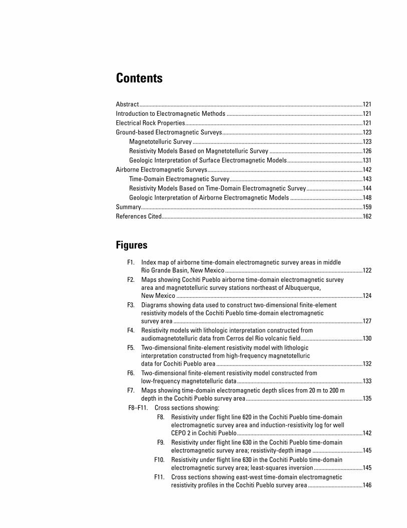
Abstract .......................................................................................................................................................121Introduction to Electromagnetic Methods ............................................................................................121Electrical Rock Properties ........................................................................................................................121Ground‑based Electromagnetic Surveys ...............................................................................................123
Magnetotelluric Survey ...................................................................................................................123Resistivity Models Based on Magnetotelluric Survey ...............................................................126Geologic Interpretation of Surface Electromagnetic Models ...................................................131
Airborne Electromagnetic Surveys .........................................................................................................142Time‑Domain Electromagnetic Survey ..........................................................................................143Resistivity Models Based on Time‑Domain Electromagnetic Survey ......................................144Geologic Interpretation of Airborne Electromagnetic Models .................................................148
Summary......................................................................................................................................................159References Cited........................................................................................................................................162
Figures F1. Index map of airborne time‑domain electromagnetic survey areas in middle
Rio Grande Basin, New Mexico .............................................................................................122 F2. Maps showing Cochiti Pueblo airborne time‑domain electromagnetic survey
area and magnetotelluric survey stations northeast of Albuquerque, New Mexico ..............................................................................................................................124
F3. Diagrams showing data used to construct two‑dimensional finite‑element resistivity models of the Cochiti Pueblo time‑domain electromagnetic survey area ................................................................................................................................127
F4. Resistivity models with lithologic interpretation constructed from audiomagnetotelluric data from Cerros del Rio volcanic field ..........................................130
F5. Two‑dimensional finite‑element resistivity model with lithologic interpretation constructed from high‑frequency magnetotelluric data for Cochiti Pueblo area ...................................................................................................132
F6. Two‑dimensional finite‑element resistivity model constructed from low‑frequency magnetotelluric data .....................................................................................133
F7. Maps showing time‑domain electromagnetic depth slices from 20 m to 200 m depth in the Cochiti Pueblo survey area ...............................................................................135
F8–F11. Cross sections showing: F8. Resistivity under flight line 620 in the Cochiti Pueblo time‑domain
electromagnetic survey area and induction‑resistivity log for well CEPO 2 in Cochiti Pueblo .....................................................................................142
F9. Resistivity under flight line 630 in the Cochiti Pueblo time‑domain electromagnetic survey area; resistivity‑depth image ..................................145
F10. Resistivity under flight line 630 in the Cochiti Pueblo time‑domain electromagnetic survey area; least‑squares inversion .................................145
F11. Cross sections showing east‑west time‑domain electromagnetic resistivity profiles in the Cochiti Pueblo survey area .....................................146
F12. Maps showing time‑domain electromagnetic elevation slices from 1,750 to 1,400 m elevation in the Cochiti Pueblo survey area ..........................................................149
F13. Cross sections showing north‑south profiles in the Cochiti Pueblo time‑domain electromagnetic survey area ..................................................................................................156
F14. Maps showing depth to surface of >100 ohm‑m resistive layer and elevation of >100 ohm‑m resistive layer in the Cochiti Pueblo time‑domain electromagnetic survey area ..................................................................................................160
Tables F1. Audiomagnetotelluric and magnetotelluric station coordinates and elevations
in the Cochiti Pueblo area, New Mexico ..............................................................................126 F2. Range of average resistivity values in regional induction logs for stratigraphic
units encountered in wells in study region ..........................................................................134 F3. Location of wells referred to in table F2 ...............................................................................134

AbstractAirborne and surface electromagnetic surveys were used
to map changes in electrical resistivity with depth in the La Bajada constriction and Cochiti Pueblo area; these changes in resistivity are related to variations in rock or deposit types that, in turn, influence aquifers in the study area. In the eastern Cerros del Rio volcanic field, the location and geometry of the northern boundary of the Cerrillos uplift are constrained by our electromagnetic survey results. This boundary defines the southeastern extent of the La Bajada constriction through which groundwater hydraulically connected with the Rio Grande flows as it passes from the Española Basin into the Santo Domingo Basin. The largely concealed Tetilla fault zone is also detected by the electromagnetic surveys in this area; it appears to form the western boundary of an east‑dipping block of electrically conductive Mancos Shale. In the north‑central part of the La Bajada constriction, a large area of lower resistivity coincides with a silt or clay lacustrine unit in upper Santa Fe Group basin‑fill deposits. In the central part of the constriction, higher resistivities correspond in part with ances‑tral Rio Grande axial gravel deposits. On the western flank of the La Bajada constriction, our electromagnetic survey results provide constraints on the relative position of basement and on the thicknesses of Paleozoic, Mesozoic, and Tertiary sedimen‑tary rocks on either side of the constriction‑bounding Pajarito fault zone.
Introduction to Electromagnetic Methods
Studies by the U.S. Geological Survey were begun in 1996 to improve understanding of the geologic framework of the Albuquerque composite basin and adjoining areas, in order that more accurate hydrogeologic parameters could be applied to new hydrologic models. The ultimate goal of this multidis‑ciplinary effort has been to better quantify estimates of future water supplies for northern New Mexico’s growing urban centers, which largely subsist on aquifers in the Rio Grande rift
basin (Bartolino and Cole, 2002). From preexisting hydrologic models it became evident that hydrogeologic uncertainties were large in the Santo Domingo Basin area, immediately upgradient from the greater Albuquerque metropolitan area, and particu‑larly in the northeast part of the basin referred to as the La Bajada constriction (see chapter A, this volume, for a geologic definition of this feature as used in this report). Accordingly, a priority for new geologic and geophysical investigations was to better determine the hydrogeologic framework of the La Bajada constriction area. This chapter along with the other chapters of this report present the results of such investigations recently conducted by the U.S. Geological Survey.
Airborne and surface electromagnetic (EM) surveys are described here as part of U.S. Geological Survey investigations of the subsurface distribution of sedimentary and volcanic rocks in the Cochiti Pueblo and La Bajada constriction areas (survey area D, fig. F1). An airborne time‑domain electromag‑netic (TDEM) survey was used to map changes in electrical resistivity with depth that are related to differences in rock type; these various rock types, in turn, affect the hydrologic properties of aquifers in the region. A ground‑based magneto‑telluric (MT) survey was used to calibrate TDEM results and to obtain electrical resistivity information from depths greater than the limits of the TDEM survey. In this chapter we discuss the electrical rock property called resistivity, the surface (MT) and airborne (TDEM) electromagnetic methods used in our study, and our approach to modeling and interpreting MT and TDEM data. We present subsurface maps and cross sections of resistivity and interpret the basic geologic framework of the study area on the basis of these data.
Electrical Rock PropertiesElectromagnetic geophysical methods detect variations
in the electrical properties of rocks—in particular electrical resistivity (or its inverse, electrical conductivity). Electri‑cal resistivity can be correlated with geologic units on the surface and at depth by using lithologic logs to provide a three‑dimensional picture of subsurface geology. The resistiv‑ity of geologic units largely depends on their fluid content,
Electromagnetic Studies and Subsurface Mapping of Electrical Resistivity in the La Bajada Constriction Area, New Mexico
By Brian D. Rodriguez, Maria Deszcz‑Pan, and David A. Sawyer

A+B
D
C
107°00’ 106°30’
35°30’
35°00’
34°30’
Rio San Jose
Rio Puerco
Rio
Gra
nde
Tijeras Arroyo
Jemez
River
Rio Puerco Santa FeRiver
TORRANCE
SOCORRO
San Acacia
VALENCIA
BERNALILLO
SANDOVAL
MC
KIN
LEY
SA
NTA
FE
Belen
Los Lunas
ALBUQUERQUE
Rio Rancho
NEW MEXICO
Areaoffigure 1
SOCORRO
EXPLANATION
Boundary of time-domainelectromagnetic survey data
Boundary of composite Albuquerque Basin
County line
County name
10 200 30 MILES
0 10 20 30 KILOMETERS
Figure F1. Airborne time‑domain electromagnetic survey areas in the middle Rio Grande Basin north of Albuquerque, New Mexico, modified from Bartolino (1999). A+B, Rio Rancho survey area. C, Rio Puerco survey area, both described in Deszcz‑Pan and others (2000). D, Cochiti Pueblo survey area discussed in this chapter.
122 Hydrogeologic Framework, La Bajada Constriction Area, Rio Grande Rift, New Mexico

porosity, fracture density, temperature, and content of conduc‑tive minerals (Keller and Frischknecht, 1966). Fluids in the pore spaces and fracture openings, especially saline fluids, can reduce resistivities in what would otherwise be a resistive rock matrix. Resistivity can also be lowered by electrically conductive clay minerals, graphitic carbon, and deposits of metallic minerals. Altered volcanic rocks commonly contain replacement minerals that have resistivities that are only a tenth of the resistivities of minerals in unaltered surrounding rocks (Nelson and Anderson, 1992). Water‑saturated clay‑rich alluvium, marine shale, and other mudstones are normally very conductive—a few (1–3) ohms per meter to a few tens (10–20) of ohms per meter. Water‑saturated, unconsolidated, terrestrial alluvial sediments are commonly moderately con‑ductive (10–70 ohm‑m). Sediments containing conglomerate and coarse, clean sand possess resistivities at the higher end of the range, and impure sand and siltstone lie at the lower end. The resistivity of water‑saturated unconsolidated sedi‑ment, at low temperature and measured at low frequencies, is controlled by the relative proportion of clay minerals, poros‑ity, interconnected pore structures, and dissolved minerals (Keller, 1987; Palacky, 1987).
Unaltered, unfractured igneous rocks are normally very resistive (typically a few hundred to thousands of ohm‑m). Carbonate rocks are moderately to highly resistive (hundreds to thousands of ohms per meter) depending upon their fluid content, porosity, fracture characteristics, and impurities. Metamorphic rocks (that do not contain graphite) are moder‑ately to highly resistive (hundreds to thousands of ohms per meter). Resistivity may be low (less than 100 ohm‑m) along fault zones that were fractured enough to have once hosted flu‑ids (generally water or brine) from which conductive minerals were deposited. Higher subsurface temperatures cause greater mobility of ions in the fluids and increase the energy level above the activation energy for electrons or ions, factors that considerably reduce rock resistivity (Keller and Frischknecht, 1966). Tables of electrical resistivity for a variety of rocks, minerals, and geologic environments may be found in Keller (1987) and Palacky (1987).
Ground-Based Electromagnetic SurveysThe MT method is a passive ground‑based electromag‑
netic geophysical technique that investigates the distribution of electrical resistivity (or its inverse, electrical conductivity) below the surface at depths of tens of meters to tens of kilome‑ters (Vozoff, 1991). It does so by measuring the Earth’s natural electric and magnetic fields. Worldwide lightning activity at frequencies of 10,000 to 1 hertz (Hz) and geomagnetic micro‑pulsations at frequencies of 1 to 0.001 Hz provide the main frequency bands used by the MT method. The natural electro‑magnetic waves propagate vertically in the Earth because the very large contrast in the resistivity of the air and the Earth causes a vertical refraction of the electromagnetic wave at the Earth’s surface (Vozoff, 1972).
The natural electric and magnetic fields are recorded in two orthogonal, horizontal directions (the vertical magnetic field is also recorded). The resulting time‑series signals are used to derive Earth‑tensor apparent resistivities and phases after first converting them to complex cross‑spectra using fast Fourier transform techniques and least‑squares, cross‑spectral analysis (Bendat and Piersol, 1971) to solve for a tensor transfer function. If one assumes that the Earth consists of a two‑input, two‑output, linear system in which the orthogonal magnetic fields are input and the orthogonal electric fields are output, then the calculated function relates the observed electric fields to the magnetic fields. Before it is converted to apparent resistivity and phase, the tensor is normally rotated into principal directions that usually correspond with the direction of maximum and minimum apparent resistivity. For a two‑dimensional Earth, the MT fields can be decoupled into transverse electric and transverse magnetic modes. Two‑dimensional resistivity modeling is generally computed to fit both modes. When the geology satisfies the two‑dimensional assumption, the MT data for the transverse electric mode are assumed to represent the electric field along geologic strike, and the data for the transverse magnetic mode are assumed to represent the electric field across strike. The MT method is well suited for studying complicated geologic environments because the electric and magnetic relations are sensitive to vertical and horizontal variations in resistivity. The method is capable of establishing whether the electromagnetic fields are responding to subsurface rock bodies of effectively one, two, or three dimensions. An introduction to the MT method and references for a more advanced understanding are contained in Dobrin and Savit (1988) and Vozoff (1991).
Magnetotelluric Survey
Six high‑frequency MT soundings (stations 1–6, table F1) were acquired in 1997 in the Cochiti Pueblo survey area (figure F2A). Spacing between soundings ranged from 4.5 to 11 km. Some stations were used to calibrate the inversion of the airborne TDEM data. These stations were located in areas that had a locally one‑dimensional TDEM response and were close to roads but distant from sources of electrical noise, such as power lines. Horizontal electric fields were sensed using titanium electrodes placed in an L‑shaped, three‑electrode array with dipole lengths of 30 m. The orthogonal, horizontal magnetic fields in the direction of the electric‑field measure‑ment array were sensed using high magnetic permeability, mu‑metal‑cored (80 percent nickel, 15 percent iron, 5 percent molybdenum) induction coils. Frequencies sampled ranged from 20,000 to 4 Hz by use of single‑station recordings of both orthogonal horizontal components of the electric and magnetic fields and of the vertical magnetic field. These fre‑quencies lie at the high end of the MT spectrum and are com‑monly referred to as audiomagnetotelluric (AMT) frequencies. Sampling these frequencies in the Cochiti Pueblo allowed us to probe the subsurface from depths of tens of meters to about one kilometer (Williams, Rodriguez, and Sampson,
Ground-Based Electromagnetic Surveys 123

A
3930
000
3932
000
3934
000
3936
000
3938
000
3940
000
3942
000
3944
000
3946
000
3948
000
3950
000
3952
000
366000 368000 370000 372000 374000 376000 378000 380000 382000 384000 386000 388000 390000 392000 394000 396000
35°3
7’30
"
NAD83 / UTM zone 13N
35°3
0’
106°22’30" 106°15’
L600
10
L60101
L60201L60301L60401L60501L60601L60701L60801L60901L61001L61101L61201L61301L61401L61501L61601L61701L61801L61901L62001L62101L62201L62301L62401L62501L62601L62701L62801L62901L63001L63101L63201L63301L63401L63501
L63601L63701L63801L63901L64001L64101L64201L64301L64401L64501L64601L64701L64801L64901L65001
L60090
L65001L64901
L64801L64701
L64601L64501
L64401L64301
L64201L64101
L64001L63901
L63801L63701
L63601L63501
L63401L63301
L63201L63101
L63001L62901
L62801L62701
L62601L62501L62401
L60090
L62301L62201L62101L62001L61901L61801L61701L61601L61501L61401L61301L61201L61101L61001L60901L60801L60701L60601L60501L60401L60301L60201L60101
L600
20
L600
30
L600
40
L600
50
L600
60
L600
70
L600
80
L600
20
L600
30
L600
40
L600
50
L600
60
L600
70
L600
80
L600
10
2,000 2,000 4,000 6,000 METERS0
Fault—Dashed where uncertain;ball on downthrown side
Flight line
Water well
Audiomagnetotelluricstation
Magnetotelluric station
Strike of resistivity
Cochiti Pueblo boundary
Power line noise(10 mV contour interval)
EXPLANATION
Santa CruzSprings
South Pajarito fault
Cam
ada fault
Tetil
la fa
ult z
one
La Bajada fault zoneCochitiReservoir
Santa Fe River
Rio Grande
Rio
Gra
nde
POWERLINE
POWERLINE
POWERLINE
POWERLINE
1
A
B
B'
A'
6
2
17
CEPO 2
4
5
1200Cochiti Lake 2
Dome Road
3
Cochiti Pueblo
10
11
8
124 Hydrogeologic Framework, La Bajada Constriction Area, Rio Grande Rift, New Mexico

Figure F2 (above and facing page). Cochiti Pueblo time‑domain electromagnetic survey area (survey area D, fig. F1) northeast of Albuquerque, New Mexico. High‑frequency magnetotelluric (AMT) sounding stations 1–6 acquired in 1997; low‑frequency magnetotelluric (MT) sounding stations 8, 10, 11, 12, and 17 acquired in 2002. A, Flight lines flown in airborne time‑domain electromagnetic survey. B, Location of AMT and MT stations. The La Bajada constriction contains Santa Fe Group basin‑fill sedimentary aquifers linking the Española and Santo Domingo Basins. Cerrillos uplift constrained by gravity data (chapter D, this volume) and by AMT stations 4 and 5 and MT stations 8, 10, and 11.
SaintPetersDome
Cerrillosuplift
35°30’
35°45’
LOS ALAMOSCOUNTY
SA
ND
OV
AL
CO
UN
TY
SA
NTA
FE
CO
UN
TY
CochitiReservoir
EXPLANATION
Audiomagnetotelluric station
Magnetotelluric station
Boundary—Time-domain eletromagneticsurvey area
106°30’ 106°15’
RioGra
nde
Santa Fe River
Galisteo Creek
25
25
La Bajadaconstriction
4
5
3
2
6
117
12
10
11
8
50 10 KILOMETERS
B
SantoDomingo
Basin
EspañolaBasin
Ground-Based Electromagnetic Surveys 125

2001). Five low‑frequency MT soundings (table F1) were also acquired in 2002 in the survey area (sites 8, 10, 11, 12 and 17), fig. F2B.
The recorded time‑series data were transformed to the frequency domain using Fourier analysis to determine a two‑dimensional apparent resistivity and phase tensor at each site. The data were rotated to maximum and minimum apparent resistivity directions so that propagation modes for the signals were decoupled into transverse electric and transverse mag‑netic modes. This treatment supplies the local strike of electri‑cal sources (illustrated by double‑headed arrows in fig. F2A). Local reference sensors were used to help reduce bias in the determinations of impedance that otherwise would be caused by noise in the instruments or the environment (Gamble, Goubau, and Clarke, 1979; Clarke and others, 1983). We also sorted cross‑power files to select optimal signal‑to‑noise data sets. Figure F3A, B shows observed data represented by digi‑tized values of the transverse electric and transverse magnetic modes from the AMT soundings after the raw data curves were smoothed (Williams, Rodriguez, and Sampson, 2001).
The effects of near‑surface resistivity anomalies can cause “static shifts” (Sternberg, Washburne, and Pellerin, 1988) in the data. Such shifts are minor in most of this data set. Only at station 4 was a static shift larger than one‑third of a log decade. At the remaining stations very minor static shifts ranged from 0.0 to less than 0.3 of a log decade. Only the large static shifts were accounted for in subsequent two‑dimensional modeling of the data.
Resistivity Models Based on Magnetotelluric Survey
The AMT data were modeled by use of a two‑ dimensional finite‑element resistivity algorithm (Wan‑namaker, Stodt, and Rijo, 1985) called PW2D. The two‑dimensional resistivity model is constructed by adjusting the resistivity values beneath the profile of AMT stations, so that for all stations the calculated two‑dimensional response agrees with the measured data. From our six AMT stations, we constructed two profiles. Profile A‑A′ (fig. F2A), at a bearing of N. 70° W., passes directly through AMT stations 6 and 3. AMT stations 1 and 2 are projected more than 1 km north and south, respectively, onto the line A‑A′. The profile B‑B′ (fig. F2A) lies between AMT stations 4 and 5 at a bear‑ing of N. 15° E. The finite‑element grid used in these models consisted of 51×26 variable‑dimension cells that extended 10 km horizontally beyond the profile end points and 2 km
Table F1. Audiomagnetotelluric and magnetotelluric station coordinates and elevations in the Cochiti Pueblo area, New Mexico.
[Coordinates are referenced to the 1866 Clarke spheroid and North American 1927 Western United States datum; stations listed in order from west to east; loca‑tions determined by use of a global positioning system; longitude and latitude format is in decimal degrees. AMT, audiomagnetotelluric; MT, magnetotelluric; UTM, Universal Transverse Mercator]
Station Type of sounding Longitude LatitudeUTM (m) Elevation
North East (m) (ft)
1 AMT –106.46612 35.67263 3,948,430 13,367,310 2,063 6,768
6 AMT –106.41874 35.66382 3,947,390 13,371,585 1,760 5,774
12 MT –106.38889 35.76750 3,958,861 13,374,449 2,380 7,808
2 AMT –106.36313 35.65193 3,946,000 13,376,600 1,740 5,709
17 MT –106.36167 35.68583 3,949,770 13,376,785 1,750 5,741
3 AMT –106.26918 35.59192 3,939,230 13,385,020 1,657 5,436
4 AMT –106.20242 35.58593 3,938,490 13,391,060 1,903 6,243
8 MT –106.20222 35.62361 3,942,655 13,391,127 2,020 6627
5 AMT –106.17803 35.66128 3,946,820 13,393,370 2,045 6,709
11 MT –106.18861 35.64639 3,945,184 13,392,391 2,025 6,644
10 MT –106.16806 35.69806 3,950,901 13,394,319 2,170 7,119
126 Hydrogeologic Framework, La Bajada Constriction Area, Rio Grande Rift, New Mexico
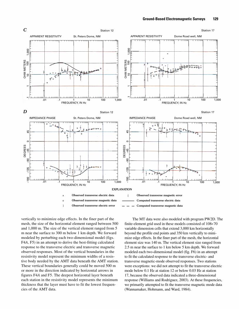
Figure F3 (facing and following 2 pages). Observed and computed data used to generate two‑dimensional finite‑element resistivity models (figs. F4A, F5, F6) in the Cochiti Pueblo time‑domain electromagnetic survey area (area D, fig. F2). A, High‑frequency magnetotelluric (AMT) observed apparent resistivity data. B, AMT observed apparent phase data. C, Low‑frequency magnetotelluric (MT) observed apparent resistivity data. D, MT observed apparent phase data.

Station 1
APPARENT RESISTIVITY Cochiti Pueblo, NM
OH
M M
ET
ER
S
FREQUENCY, IN Hz
.11
1010
01,
000
10 100 1,000 10,000 100,000
Station 6
APPARENT RESISTIVITY Cochiti Pueblo, NM
OH
M M
ET
ER
S
FREQUENCY, IN Hz
.11
1010
01,
000
10 100 1,000 10,000 100,000
Station 2
APPARENT RESISTIVITY Cochiti Pueblo, NM
OH
M M
ET
ER
S
FREQUENCY, IN Hz
.11
1010
01,
000
10 100 1,000 10,000 100,000
Station 3
APPARENT RESISTIVITY Cochiti Pueblo, NM
OH
M M
ET
ER
S
FREQUENCY, IN Hz
.11
1010
01,
000
10 100 1,000 10,000 100,000
Station 4
APPARENT RESISTIVITY Cochiti Pueblo, NM
OH
M M
ET
ER
S
FREQUENCY, IN Hz
.11
1010
01,
000
10 100 1,000 10,000 100,000
Station 5
APPARENT RESISTIVITY Cochiti Pueblo, NM
OH
M M
ET
ER
S
FREQUENCY, IN Hz
.11
1010
01,
000
10 100 1,000 10,000 100,000
A
EXPLANATION
Observed transverse electric data
Observed transverse magnetic data
Observed transverse electric error
x
o
]
Computed transverse electric data
Computed transverse magnetic data
Observed transverse magnetic error[
Ground-Based Electromagnetic Surveys 127

Station 1
IMPEDANCE PHASE Cochiti Pueblo, NM
DE
GR
EE
S
FREQUENCY, IN Hz
–180
–135
–90
–45
045
10 100 1,000 10,000 100,000
Station 6
IMPEDANCE PHASE Cochiti Pueblo, NM
DE
GR
EE
S
FREQUENCY, IN Hz10 100 1,000 10,000 100,000
Station 2
IMPEDANCE PHASE Cochiti Pueblo, NM
DE
GR
EE
S
FREQUENCY, IN Hz10 100 1,000 10,000 100,000
Station 3
IMPEDANCE PHASE Cochiti Pueblo, NM
DE
GR
EE
S
FREQUENCY, IN Hz10 100 1,000 10,000 100,000
Station 4
IMPEDANCE PHASE Cochiti Pueblo, NM
DE
GR
EE
S
FREQUENCY, IN Hz10 100 1,000 10,000 100,000
Station 5
IMPEDANCE PHASE Cochiti Pueblo, NM
DE
GR
EE
S
FREQUENCY, IN Hz10 100 1,000 10,000 100,000
–180
–135
–90
–45
045
–180
–135
–90
–45
045
–180
–135
–90
–45
045
–180
–135
–90
–45
045
–180
–135
–90
–45
045
EXPLANATION
Observed transverse electric data
Observed transverse magnetic data
Observed transverse electric error
x
o
]
Computed transverse electric data
Computed transverse magnetic data
Observed transverse magnetic error[
B
128 Hydrogeologic Framework, La Bajada Constriction Area, Rio Grande Rift, New Mexico
Station 12
IMPEDANCE PHASE St. Peters Dome, NM
FREQUENCY, IN Hz.01 .1 1 10 100 1,000
Station 17
IMPEDANCE PHASE Dome Road well, NM
EXPLANATION
Observed transverse electric data
Observed transverse magnetic data
Observed transverse electric error
x
o
]
Computed transverse electric data
Computed transverse magnetic data
Observed transverse magnetic error[
DE
GR
EE
S–1
80–1
35–9
0–4
50
45
DE
GR
EE
S–1
80–1
35–9
0–4
50
45
FREQUENCY, IN Hz.01 .1 1 10 100 1,000
Station 12
APPARENT RESISTIVITY St. Peters Dome, NM
OH
M M
ET
ER
S
FREQUENCY, IN Hz
.11
1010
01,
000
.01 101.1 100 1,000
Station 17
APPARENT RESISTIVITY Dome Road well, NM
FREQUENCY, IN Hz.01 .1 1 10 1,000100
C
D
OH
M M
ET
ER
S.1
110
100
1,00
0
vertically to minimize edge effects. In the finer part of the mesh, the size of the horizontal element ranged between 500 and 1,000 m. The size of the vertical element ranged from 5 m near the surface to 300 m below 1 km depth. We forward modeled by perturbing each two‑dimensional model (figs. F4A, F5) in an attempt to derive the best‑fitting calculated response to the transverse electric and transverse magnetic observed responses. Most of the vertical boundaries in the resistivity model represent the minimum widths of a resis‑tive body needed by the AMT data beneath the AMT station. These vertical boundaries generally could be moved 500 m or more in the direction indicated by horizontal arrows in figures F4A and F5. The deepest horizontal layer beneath each station in the resistivity model represents the minimum thickness that the layer must have to fit the lowest frequen‑cies of the AMT data.
The MT data were also modeled with program PW2D. The finite‑element grid used in these models consisted of 108×70 variable dimension cells that extend 3,000 km horizontally beyond the profile end points and 350 km vertically to mini‑mize edge effects. In the finer part of the mesh, the horizontal element size was 140 m. The vertical element size ranged from 2.5 m near the surface to 1 km below 5 km depth. We forward modeled each two‑dimensional model (fig. F6) in an attempt to fit the calculated response to the transverse electric‑ and transverse magnetic‑mode observed responses. Two stations were exceptions: we did not attempt to fit the transverse electric mode below 0.1 Hz at station 12 or below 0.03 Hz at station 17, because the observed data indicated a three‑dimensional response (Williams and Rodriguez, 2003). At these frequencies, we primarily attempted to fit the transverse magnetic mode data (Wannamaker, Hohmann, and Ward, 1984).
Ground-Based Electromagnetic Surveys 129

0
4100
DEP
TH, I
N M
ETER
S
1,200
1,100
1,000
900
800
700
600
500
400
300
200
Cerrillos del Rio Volcanic FieldB
A
B'
0 1 2 3 4 5 6 7 8
Mancos Shale ?
Mancos Shale ?
?
(2)
(10)
?
?
?
(5)
(2)
(10)
(2)
(300)(100) Basalt
Basalt(1,000)
(100)
?
(100) Dry Santa Fe (?) Group ?
Saturated Santa Fe (?) Group
(20)
Feeder dike?(10,000)
5
1200-Footwell
Fau
lt ?
Fau
lt ?
DISTANCE, IN KILOMETERS
EXPLANATION
Audiomagnetotelluric stationMedium grain size
Fine grain size
Water well
Resistivity—In ohm-m(10)
130 Hydrogeologic Framework, La Bajada Constriction Area, Rio Grande Rift, New Mexico

Clay
Basalt
Clay cinders
Redalluvium +
basaltcinders
Gray hardbasalt
Red andyellow
sandy silt+ black cinders
Basalt
Basalt
Basalt
Basalt
Basalt
Clay
7686
155
306
413
440447
604
630
762
Ash800
840
880
988
Sandy silt + gravel—Topof producing zone1,054
1,090
1,115
1,163
1,2041,207
Sandy silt—Base ofproducing zone
15
23
184
192
Clay
125
256
268
301
307
354
368
93
47
332
340
812
SWL = –1,007 ftElevation = 5,718 ft
Depth(ft)
LithologyDepth(m)
Clay + gravel
Sand + gravel
Sandy silt, interbeddedcobble gravel
Sand
50(100)
(100)
(1,000)
(20)
(20)
AMT−51200-Foot WellB Figure F4 (left and facing page). A, Two‑dimensional
finite‑element resistivity model (with lithologic interpretation) constructed from high‑frequency magnetotelluric (AMT) data for the Cerros del Rio volcanic field profile B‑B′ (fig. F2A) in the Cochiti Pueblo time‑domain electromagnetic survey area. Arrows within the model indicate uncertainty in the placement of boundaries. Vertical exaggeration is 10. B, Comparison of the resistivity model of AMT data at station 5 (fig. F4A) and lithology of the 1200‑Foot well. Locations of AMT station 5 and 1200‑Foot well shown on figure F2A.
The calculated fits of our two‑dimensional resistivity models (figs. F4A, F5, F6) are shown in figure F3. Resistivity boundaries in the model are only approximate because all of the AMT stations are separated by more than 1 km, and the MT stations are separated by more than 8 km. Because of the wide spacing of stations, undetected rock units or structures may exist between stations that are not identified in the resistivity model.
Geologic Interpretation of Surface Electromagnetic Models
Geologic interpretations are based on the resistivity structures revealed in the modeled AMT and MT data (figs. F4A, F5, F6) and on regional induction log resistivities of saturated geologic units in seven wells (tables F2, F3): Dome Road (fig. F2A), CEPO 2 (fig. F2A), Pelto Ortiz 1 (fig. A3), Pelto Blackshare 1 (fig. A3), Black Oil Ferrill 5 (fig. A3), Transocean McKee 1 (fig. A3), and Shell Laguna Wilson Trust 1 (south of our survey area). The northerly electrical strike directions in figure F2A can be considered a function of the prominent structural grain of those geologic units, the approximate trend of the shallow geologic structure near the AMT stations (figs. F4A, F5), and the approximate struc‑tural trend in the upper few kilometers of crust near the MT stations (fig. F6).
As described in chapter A (this volume), the Cochiti Pueblo study area is subdivided into three principal geologic ter‑ranes: the western Saint Peters Dome uplifted block, the central subsided La Bajada constriction, and the eastern Cerrillos uplift (fig. A4). AMT and MT stations 1 and 12 are in the western part of the Saint Peters Dome block, in volcanic rocks of the southeastern Jemez volcanic field; stations 2, 3, 6, and 17 are in the northeast part of the Santo Domingo Basin in the central part of the La Bajada constriction; and stations 4 and 5 lie along the northern border of the Cerrillos uplift (figs. F2B, A4).
The south‑north profile, B‑B′ (fig. F2A), in the eastern Cerros del Rio volcanic field terrane, shows a moderately resistive basalt (100–300 ohm‑m) exposed at the surface that has a thickness of 60±10 m beneath station 4 (fig. F4A). Beneath the basalt, a very conductive interval (3 ohm‑m) that is 20±10 m thick may be a lacustrine mudstone sequence in
Ground-Based Electromagnetic Surveys 131

2,1001
ELEV
ATI
ON
, IN
MET
ERS
600
800
900
1,000
1,100
1,200
1,300
1,400
1,500
1,600
1,700
1,800
1,900
2,000
A A'
0 5 10 15DISTANCE, IN KILOMETERS
?
(100)
(100)
(100)
(10)
RioGrande
TentRocks
Cochiti Pueblo
Cam
ada
fau
lt
So
uth
Paj
arit
o f
ault
CEPO 2 (Projected)
26
3
(10)
(2)
(100)
(30)
(10)
Volcanic Rocks (?)
SaturatedSanta Fe (?)
Group(30)
SaturatedSanta Fe (?)
Group(30)
SaturatedSanta Fe (?)
Group(30)
Volcanic Rocks (?)
Volcanic Rocks(300)
Mancos Shale ?
Bas
alti
c ve
nt
?
?
? ?
(10)
?
?
??
EXPLANATION
Audiomagnetotelluric stationMedium grain size
Fine grain size
Water well
Resistivity—In ohm-m(10)
Figure F5. Two‑dimensional finite‑element resistivity model (with lithologic interpretation) from high‑frequency magnetotelluric (AMT) data for the Cochiti Pueblo profile (A‑A′, fig. F2A) in the Cochiti Pueblo time‑domain electromagnetic survey area. Arrow near question mark within the model indicates uncertainty in placement of boundary. Vertical exaggeration is 20.
132 Hydrogeologic Framework, La Bajada Constriction Area, Rio Grande Rift, New Mexico

the upper part of the Santa Fe Group. This conductive inter‑val is underlain by moderately conductive rocks (10 ohm‑m); those rocks, which probably include a saturated, fine‑grained Santa Fe interval, volcaniclastic Oligocene Espinaso Forma‑tion, and possibly the Eocene Galisteo Formation sedimentary rocks, have a composite thickness of 100±20 m. Some part of the weathered Mancos Shale could be included within this 10‑ohm‑m zone below the basalt. However, the very conductive horizon (2 ohm‑m) beginning at a depth of 180±20 m below the AMT station is likely clay‑rich Cretaceous marine deposits of the Mancos Shale. Preliminary MT models of this sounding show that the conductive interval is 620±80 m thick. Beneath this very conductive interval, less conductive rocks (5 ohm‑m) probably include units of Permian, Triassic, and Jurassic sedi‑mentary rocks.
A resistive interval of basalts (1,000 ohm‑m) of the Cerros del Rio at station 5 (fig. F4A) are 250±25 m thick. This basalt interval ranges from 60 to 250 m thick between stations 4 and 5. Approximately 140 m of the 250 m basalt thickness at station 5 reflects constructional topography resulting from the growth of basaltic volcanoes. A remark‑ably detailed driller’s log (fig. F4B) exists for a water well (the 1200‑Foot well) 200 m northwest of AMT station 5. The thickness of the basalt (256 m) measured on a lithology log constructed from the driller’s record corresponds closely with the thickness of basalt determined in the AMT model (250±25 m). As recorded in the driller’s log, the static water elevation lay at 307 m depth, so our forward modeling used a value of 100 ohm‑m for the unsaturated Santa Fe Group sand and gravel above the water table. Saturated sand and silty sand of the Santa Fe Group typically have resistivities in the 20–70 ohm‑m range. The modeled electrical sounding shows that 20 ohm‑m material extends to a depth of 900±100 m. Beneath the 20 ohm‑m material is a 10 ohm‑m interval with a thickness of 250±100 m. The 10 ohm‑m material may include early Tertiary Galisteo and Espinaso Formations that cannot be separated from Santa Fe Group solely on the basis of their electrical signatures. Espinaso Formation is found in the Yates La Mesa petroleum test well 2 (10 km to the northeast, north of the Santa Fe River, pl. 2), but deposits of the Galisteo may have been eroded or never deposited to the north. Very conductive (2 ohm‑m) inferred Mancos Shale occurs at a depth of 1,150±100 m and has lower electrical resistivity than other units in the region. Between station 4, where the top of the Mancos is 1,700 m above sea level, and station 5, where it is 900 m, the top of the Mancos appar‑ently drops 800 m. Thus, these MT results provide evidence for 800 m of Tertiary structural relief at the north end of the Cerrillos uplift. The shallow Mancos Shale located at AMT station 4, immediately south of Tetilla Peak, provides the
(20)
(50)
(10)
(10)
(2–10)
(200)
(200)
?
(200)
MT–12
1,000
0
2,000
3,000
(20)
MT–17
1,000
0
2,000
3,000
?
DE
PT
H, I
N M
ET
ER
S
DE
PT
H, I
N M
ET
ER
S
Figure F6. Two‑dimensional finite‑element resistivity model from low‑frequency magnetotelluric (MT) data for MT sounding stations 12 and 17 (see fig. F2B for locations). Arrow near question mark within the model indicates uncertainty in placement of boundary.
Ground-Based Electromagnetic Surveys 133

Table F2. Range of average resistivity values in regional induction logs for stratigraphic units intersected in wells in study region.
[Well abbreviations: B, Black Oil Ferrill 5; C, CEPO 2; D, Dome Road; PB, Pelto Blackshare 1; PO, Pelto Ortiz 1; T, Transocean McKee 1; S, Shell Laguna Wilson Trust 1]
Epoch or Period Stratigraphic unit or level Ohm-m Thickness (m) Well
Pliocene−Miocene Santa Fe Group 8–70 400–451 D, PB, C
Oligocene Espinaso Formation 10–20 533 PB
Eocene Galisteo Formation 5–20 526–1,376 PB, PO, B
Cretaceous Upper 2–40 420–1,526 PB, PO, B, S, T
Jurassic Upper/Middle 2–20 223–453 PB, S, T
Triassic Upper 2–15 482–933 S, T
Permian Upper/Lower 6–200 262–659 S, T
Pennsylvanian Upper/Middle/Lower 7–200 585–766 S, T
Table F3. Location of wells referred to in table F2.
[Coordinates listed below are referenced to the 1866 Clarke spheroid and North American 1927 datum; stations listed in order from west to east; locations determined using a global positioning system; longitude and latitude format is decimal degrees; UTM, Universal Transverse Mercator]
Well Longitude LatitudeUTM (m) Elevation
North East (m) (ft)
B –106.041 35.386 3,916,149 13,405,451 1,787 5,889
C –106.351 35.627 3,943,183 13,377,650 1,632 5,379
D –106.365 35.683 3,949,468 13,376,462 1,765 5,818
PB –106.269 35.397 3,917,611 13,384,758 1,831 6,034
PO –106.058 35.412 3,919,049 13,403,938 1,761 5,804
T –105.990 35.390 3,916,545 13,410,088 1,801 5,935
S –106.968 35.024 3,877,277 13,320,453 1,643 5,415
farthest northwest constraint for the edge of the Cerrillos uplift. This AMT‑defined northwest edge is consistent with the subsurface extent of the uplift on the basis of gravity data (chapter D, this volume). The feeder dike shown in figure F4A may be oriented in any one of several azimuthal directions with respect to station 5. It could correspond with dikes associated with the Cerro Colorado vent to the west (fig. F7A), the Cerrito Portrillo andesite volcano to the northeast (pl. 2), or a N. 20° E.–trending linear chain of younger basalts and andesites to the southeast (pl. 2). The high accuracy of the thickness of resistive basalt determined by the sounding at AMT station 5, as compared with the driller’s log for the 1200‑Foot well, suggests that electrical soundings of this type may be an accurate method of deter‑mining the thickness of volcanic deposits in the Cerros del Rio volcanic field and in similar settings underlain by shallow volcanic rocks of variable thickness. The advantage of the ground AMT soundings is the much greater depth of investigation, as much as 1,200 m in the AMT station 5 example, as opposed to a maximum depth of about 300 m
depth for the airborne TDEM data in a favorable situation (for example, no thick, shallow conductors). Detailed com‑parison of the AMT data from station 5 with the lithologic log from the 1200‑Foot well (fig. F4B) also provides some insight into the degree of resolution of the AMT soundings and plan‑mapping techniques: Modeling of the AMT data was able to resolve the thickness of resistive basalt only to within 10 percent. Also, in the upper 47 m, we were not able to distinguish the 24‑m interval of dry basalt cinders from
134 Hydrogeologic Framework, La Bajada Constriction Area, Rio Grande Rift, New Mexico
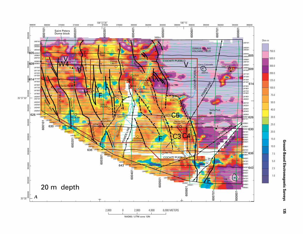
Figure F7 (facing and following 5 pages). Depth slices in the Cochiti Pueblo time‑domain electromagnetic survey area (A–F), drawn on the basis of least‑squares inversions. Solid numbered triangles represent high‑frequency magnetotelluric sounding stations. C3, C4, C5, W4, magnetic anomalies discussed in chapter D (this volume); F, inferred fine grain size sediments; V, inferred volcanic rock. A, 20‑m‑depth slice. B, 50‑m‑depth slice. C, 70‑m‑depth slice. D, 100‑m‑depth slice. E, 150‑m‑depth slice. F, 200‑m‑depth slice.
VV
F
F
F20 m depth
W4
C4
C5
C3
3930
000
3932
000
3934
000
3936
000
3938
000
3940
000
3942
000
3944
000
3946
000
3948
000
3950
000
3952
000
366000 368000 370000 372000 374000 376000 378000 380000 382000 384000 386000 388000 390000 392000 394000 396000
L65001L65001
L64901L64901
L64801 L64801
L64701 L64701
L64601L64601
L64501L64501
L64401L64401
L64301L64301
L64201L64201
L64101L64101
L64001L64001
L63901L63901
L63801L63801
L63701
L63701
L63601L63601
L63501 L63501
L63401L63401
L63301L63301
L63201
L63201
L63101L63101
L63001
L63001
L62901
L62901
L62801
L62801
L62701L62701
L62601L62601
L62501
L62501
L62401
L62401
L62301
L62301
L62201
L62201
L62101
L62101
L62001L62001
L61901
L61901
L61801L61801
L61701
L61701
L61601
L61601
L61501
L61501
L61401
L61401
L61301
L61301
L61201
L61201
L61101
L61101
L61001L61001
L60901
L60901
L60801
L60801
L60701
L60701
L60601
L60601
L60501
L60501
L60401
L60401
L60301
L60301
L60201L60201
L60101L60101
605605
609
614
626
630
638
643643
638
630
626
614
609
6001
0160
0101
6002
0160
0201
6003
0160
0301
6004
0160
0401
6005
0160
0501
6006
01
6006
01
6007
0160
0701
6008
0160
0801
NAD83 / UTM zone 13N
0 2,000 4,000 6,000 METERS2,000
Cerro Colorado
2227m
COCHITI PUEBLO
COCHITI PUEBLOC
OC
HIT
I PU
EB
LO
CO
CH
ITI P
UE
BLO
Santa Fe NF
So
uth
Pajarito
fault
Cochiti fault
CochitiLake
Tetilla PeakLa B
ajada fault
La Bajada fault
La Bajada fault
Sile fault
Cam
ada fault
Peralta fault
Cochiti
Sanchez fault
Sanchez fault
Sanchez fault
I-25
POWER LINE
POW
ER L
INE
POW
ER L
INE
POW
ER L
INE
1
6
2
4
5
3
CERROS DEL RIOVOLCANIC FIELD
Cañada de
Santa Fe
Santa
FeRiver
CochitiReservoir
Rio
Gra
nde
Rio Gran
de
San Francisco fault
Tetil
la fa
ult
Saint PetersDome block
A
1.0
2.5
5.0
7.5
10.0
15.0
20.0
25.0
30.0
40.0
50.0
75.0
100.0
125.0
200.0
300.0
500.0
750.0
Ohm-m1609m
1583m
35°30’
35°37’30”
106°22’30” 106°15’
Santa CruzSprings Tract
Blow-TW
1200 well
Solar-TWCOE
TetillaCOE
CEPO 2
C1
C2
CEPO 3(Peralta)
2BW
CEPO 1(Landfill)
3-TW
CochitiElementary
180-TW
4-TW
CochitiLake 2
DomeRoad
TentRocks
170TW
2Cochiti-TW
800'well
1
Ground-Based Electromagnetic Surveys
135

VV
F
F
F50 m depth
W4
C4
C5
C3
3930
000
3932
000
3934
000
3936
000
3938
000
3940
000
3942
000
3944
000
3946
000
3948
000
3950
000
3952
000
366000 368000 370000 372000 374000 376000 378000 380000 382000 384000 386000 388000 390000 392000 394000 396000
L65001L65001
L64901L64901
L64801 L64801
L64701 L64701
L64601L64601
L64501L64501
L64401L64401
L64301L64301
L64201L64201
L64101L64101
L64001L64001
L63901L63901
L63801L63801
L63701
L63701
L63601L63601
L63501 L63501
L63401L63401
L63301L63301
L63201
L63201
L63101L63101
L63001
L63001
L62901
L62901
L62801
L62801
L62701L62701
L62601L62601
L62501
L62501
L62401
L62401
L62301
L62301
L62201
L62201
L62101
L62101
L62001L62001
L61901
L61901
L61801L61801
L61701
L61701
L61601
L61601
L61501
L61501
L61401
L61401
L61301
L61301
L61201
L61201
L61101
L61101
L61001L61001
L60901
L60901
L60801
L60801
L60701
L60701
L60601
L60601
L60501
L60501
L60401
L60401
L60301
L60301
L60201L60201
L60101L60101
605605
609
614
626
630
638
643643
638
630
626
614
609
6001
0160
0101
6002
0160
0201
6003
0160
0301
6004
0160
0401
6005
0160
0501
6006
01
6006
01
6007
0160
0701
6008
0160
0801
NAD83 / UTM zone 13N
0 2,000 4,000 6,000 METERS2,000
Cerro Colorado
2227m
COCHITI PUEBLO
COCHITI PUEBLOC
OC
HIT
I PU
EB
LO
CO
CH
ITI P
UE
BLO
Santa Fe NF
So
uth
Pajarito
fault
Cochiti fault
CochitiLake
Tetilla Peak
La Bajada fault
La Bajada fault
La Bajada fault
Sile fault
Cam
ada fault
Peralta fault
Cochiti
Sanchez fault
Sanchez fault
Sanchez fault
I-25
POWER LINE
POW
ER L
INE
POW
ER L
INE
POW
ER L
INE
1
6
2
4
5
3
CERROS DEL RIOVOLCANIC FIELD
Cañada de
Santa Fe
Santa
FeRiver
CochitiReservoir
Rio
Gra
nde
Rio Gran
de
San Francisco fault
Tetil
la fa
ult
Saint PetersDome block
B
1.0
2.5
5.0
7.5
10.0
15.0
20.0
25.0
30.0
40.0
50.0
75.0
100.0
125.0
200.0
300.0
500.0
750.0
Ohm-m1609m
1583m
35°30’
35°37’30”
106°22’30” 106°15’
Santa CruzSprings Tract
Blow-TW
1200 well
Solar-TWCOE
TetillaCOE
CEPO 2
C1
C2
CEPO 3(Peralta)
2BW
CEPO 1(Landfill)
3-TW
CochitiElementary
180-TW
4-TW
CochitiLake 2
DomeRoad
TentRocks
170TW
2Cochiti-TW
800'well
1
136
Hydrogeologic Framew
ork, La Bajada Constriction Area, Rio Grande Rift, New
Mexico

VV
F
F
F70 m depth
W4
C4
C5
C3
3930
000
3932
000
3934
000
3936
000
3938
000
3940
000
3942
000
3944
000
3946
000
3948
000
3950
000
3952
000
366000 368000 370000 372000 374000 376000 378000 380000 382000 384000 386000 388000 390000 392000 394000 396000
L65001L65001
L64901L64901
L64801 L64801
L64701 L64701
L64601L64601
L64501L64501
L64401L64401
L64301L64301
L64201L64201
L64101L64101
L64001L64001
L63901L63901
L63801L63801
L63701
L63701
L63601L63601
L63501 L63501
L63401L63401
L63301L63301
L63201
L63201
L63101L63101
L63001
L63001
L62901
L62901
L62801
L62801
L62701L62701
L62601L62601
L62501
L62501
L62401
L62401
L62301
L62301
L62201
L62201
L62101
L62101
L62001L62001
L61901
L61901
L61801L61801
L61701
L61701
L61601
L61601
L61501
L61501
L61401
L61401
L61301
L61301
L61201
L61201
L61101
L61101
L61001L61001
L60901
L60901
L60801
L60801
L60701
L60701
L60601
L60601
L60501
L60501
L60401
L60401
L60301
L60301
L60201L60201
L60101L60101
605605
609
614
626
630
638
643643
638
630
626
614
609
6001
0160
0101
6002
0160
0201
6003
0160
0301
6004
0160
0401
6005
0160
0501
6006
01
6006
01
6007
0160
0701
6008
0160
0801
NAD83 / UTM zone 13N
0 2,000 4,000 6,000 METERS2,000
Cerro Colorado
2227m
COCHITI PUEBLO
COCHITI PUEBLOC
OC
HIT
I PU
EB
LO
CO
CH
ITI P
UE
BLO
Santa Fe NF
So
uth
Pajarito
fault
Cochiti fault
CochitiLake
Tetilla PeakLa B
ajada fault
La Bajada fault
La Bajada fault
Sile fault
Cam
ada fault
Peralta fault
Cochiti
Sanchez fault
Sanchez fault
Sanchez fault
I-25
POWER LINE
POW
ER L
INE
POW
ER L
INE
POW
ER L
INE
1
6
2
4
5
3
CERROS DEL RIOVOLCANIC FIELD
Cañada de
Santa Fe
Santa
FeRiver
CochitiReservoir
Rio
Gra
nde
Rio Gran
de
San Francisco fault
Tetil
la fa
ult
Saint PetersDome block
C
1.0
2.5
5.0
7.5
10.0
15.0
20.0
25.0
30.0
40.0
50.0
75.0
100.0
125.0
200.0
300.0
500.0
750.0
Ohm-m1609m
1583m
35°30’
35°37’30”
106°22’30” 106°15’
Santa CruzSprings Tract
Blow-TW
1200 well
Solar-TWCOE
TetillaCOE
CEPO 2
C1
C2
CEPO 3(Peralta)
2BW
CEPO 1(Landfill)
3-TW
CochitiElementary
180-TW
4-TW
CochitiLake 2
DomeRoad
TentRocks
170TW
2Cochiti-TW
800'well
1
Ground-Based Electromagnetic Surveys
137

VV
F
F
F100 m depth
W4
C4
C5
C3
3930
000
3932
000
3934
000
3936
000
3938
000
3940
000
3942
000
3944
000
3946
000
3948
000
3950
000
3952
000
366000 368000 370000 372000 374000 376000 378000 380000 382000 384000 386000 388000 390000 392000 394000 396000
L65001L65001
L64901L64901
L64801 L64801
L64701 L64701
L64601L64601
L64501L64501
L64401L64401
L64301L64301
L64201L64201
L64101L64101
L64001L64001
L63901L63901
L63801L63801
L63701
L63701
L63601L63601
L63501 L63501
L63401L63401
L63301L63301
L63201
L63201
L63101L63101
L63001
L63001
L62901
L62901
L62801
L62801
L62701L62701
L62601L62601
L62501
L62501
L62401
L62401
L62301
L62301
L62201
L62201
L62101
L62101
L62001L62001
L61901
L61901
L61801L61801
L61701
L61701
L61601
L61601
L61501
L61501
L61401
L61401
L61301
L61301
L61201
L61201
L61101
L61101
L61001L61001
L60901
L60901
L60801
L60801
L60701
L60701
L60601
L60601
L60501
L60501
L60401
L60401
L60301
L60301
L60201L60201
L60101L60101
605605
609
614
626
630
638
643643
638
630
626
614
609
6001
0160
0101
6002
0160
0201
6003
0160
0301
6004
0160
0401
6005
0160
0501
6006
01
6006
01
6007
0160
0701
6008
0160
0801
NAD83 / UTM zone 13N
0 2,000 4,000 6,000 METERS2,000
Cerro Colorado
2227m
COCHITI PUEBLO
COCHITI PUEBLOC
OC
HIT
I PU
EB
LO
CO
CH
ITI P
UE
BLO
Santa Fe NF
So
uth
Pajarito
fault
Cochiti fault
CochitiLake
Tetilla Peak
La Bajada fault
La Bajada fault
La Bajada fault
Sile fault
Cam
ada fault
Peralta fault
Cochiti
Sanchez fault
Sanchez fault
Sanchez fault
I-25
POWER LINE
POW
ER L
INE
POW
ER L
INE
POW
ER L
INE
1
6
2
4
5
3
CERROS DEL RIOVOLCANIC FIELD
Cañada de
Santa Fe
Santa
FeRiver
CochitiReservoir
Rio
Gra
nde
Rio Gran
de
San Francisco fault
Tetil
la fa
ult
Saint PetersDome block
D
1.0
2.5
5.0
7.5
10.0
15.0
20.0
25.0
30.0
40.0
50.0
75.0
100.0
125.0
200.0
300.0
500.0
750.0
Ohm-m1609m
1583m
35°30’
35°37’30”
106°22’30” 106°15’
Santa CruzSprings Tract
Blow-TW
1200 well
Solar-TWCOE
TetillaCOE
CEPO 2
C1
C2
CEPO 3(Peralta)
2BW
CEPO 1(Landfill)
3-TW
CochitiElementary
180-TW
4-TW
CochitiLake 2
DomeRoad
TentRocks
170TW
2Cochiti-TW
800'well
1
Larg
e ar
ea o
f silt
/cla
y
lacu
strin
e se
dim
ents
?
138
Hydrogeologic Framew
ork, La Bajada Constriction Area, Rio Grande Rift, New
Mexico

VV
F
F
F150 m depth
W4
C4
C5
C3
3930
000
3932
000
3934
000
3936
000
3938
000
3940
000
3942
000
3944
000
3946
000
3948
000
3950
000
3952
000
366000 368000 370000 372000 374000 376000 378000 380000 382000 384000 386000 388000 390000 392000 394000 396000
L65001L65001
L64901L64901
L64801 L64801
L64701 L64701
L64601L64601
L64501L64501
L64401L64401
L64301L64301
L64201L64201
L64101L64101
L64001L64001
L63901L63901
L63801L63801
L63701
L63701
L63601L63601
L63501 L63501
L63401L63401
L63301L63301
L63201
L63201
L63101L63101
L63001
L63001
L62901
L62901
L62801
L62801
L62701L62701
L62601L62601
L62501
L62501
L62401
L62401
L62301
L62301
L62201
L62201
L62101
L62101
L62001L62001
L61901
L61901
L61801L61801
L61701
L61701
L61601
L61601
L61501
L61501
L61401
L61401
L61301
L61301
L61201
L61201
L61101
L61101
L61001L61001
L60901
L60901
L60801
L60801
L60701
L60701
L60601
L60601
L60501
L60501
L60401
L60401
L60301
L60301
L60201L60201
L60101L60101
605605
609
614
626
630
638
643643
638
630
626
614
609
6001
0160
0101
6002
0160
0201
6003
0160
0301
6004
0160
0401
6005
0160
0501
6006
01
6006
01
6007
0160
0701
6008
0160
0801
NAD83 / UTM zone 13N
0 2,000 4,000 6,000 METERS2,000
Cerro Colorado
2227m
COCHITI PUEBLO
COCHITI PUEBLOC
OC
HIT
I PU
EB
LO
CO
CH
ITI P
UE
BLO
Santa Fe NF
So
uth
Pajarito
fault
Cochiti fault
CochitiLake
Tetilla PeakLa B
ajada fault
La Bajada fault
La Bajada fault
Sile fault
Cam
ada fault
Peralta fault
Cochiti
Sanchez fault
Sanchez fault
Sanchez fault
I-25
POWER LINE
POW
ER L
INE
POW
ER L
INE
POW
ER L
INE
1
6
2
4
5
3
CERROS DEL RIOVOLCANIC FIELD
Cañada de
Santa Fe
Santa
FeRiver
CochitiReservoir
Rio
Gra
nde
Rio Gran
de
San Francisco fault
Tetil
la fa
ult
Saint PetersDome block
E
1.0
2.5
5.0
7.5
10.0
15.0
20.0
25.0
30.0
40.0
50.0
75.0
100.0
125.0
200.0
300.0
500.0
750.0
Ohm-m1609m
1583m
35°30’
35°37’30”
106°22’30” 106°15’
Santa CruzSprings Tract
Blow-TW
1200 well
Solar-TWCOE
TetillaCOE
CEPO 2
C1
C2
CEPO 3(Peralta)
2BW
CEPO 1(Landfill)
3-TW
CochitiElementary
180-TW
4-TW
CochitiLake 2
DomeRoad
TentRocks
170TW
2Cochiti-TW
800'well
1
Larg
e ar
ea o
f silt
/cla
y
lacu
strin
e se
dim
ents
?
Ground-Based Electromagnetic Surveys
139

VV
F
F
F200 m depth
W4
C4
C5
C3
3930
000
3932
000
3934
000
3936
000
3938
000
3940
000
3942
000
3944
000
3946
000
3948
000
3950
000
3952
000
366000 368000 370000 372000 374000 376000 378000 380000 382000 384000 386000 388000 390000 392000 394000 396000
L65001L65001
L64901L64901
L64801 L64801
L64701 L64701
L64601L64601
L64501L64501
L64401L64401
L64301L64301
L64201L64201
L64101L64101
L64001L64001
L63901L63901
L63801L63801
L63701
L63701
L63601L63601
L63501 L63501
L63401L63401
L63301L63301
L63201
L63201
L63101L63101
L63001
L63001
L62901
L62901
L62801
L62801
L62701L62701
L62601L62601
L62501
L62501
L62401
L62401
L62301
L62301
L62201
L62201
L62101
L62101
L62001L62001
L61901
L61901
L61801L61801
L61701
L61701
L61601
L61601
L61501
L61501
L61401
L61401
L61301
L61301
L61201
L61201
L61101
L61101
L61001L61001
L60901
L60901
L60801
L60801
L60701
L60701
L60601
L60601
L60501
L60501
L60401
L60401
L60301
L60301
L60201L60201
L60101L60101
605605
609
614
626
630
638
643643
638
630
626
614
609
6001
0160
0101
6002
0160
0201
6003
0160
0301
6004
0160
0401
6005
0160
0501
6006
01
6006
01
6007
0160
0701
6008
0160
0801
NAD83 / UTM zone 13N
0 2,000 4,000 6,000 METERS2,000
Cerro Colorado
2227m
COCHITI PUEBLO
COCHITI PUEBLO
CO
CH
ITI P
UE
BLO
CO
CH
ITI P
UE
BLO
Santa Fe NF
So
uth
Pajarito
fault
Cochiti fault
CochitiLake
Tetilla Peak
La Bajada fault
La Bajada fault
La Bajada fault
Sile fault
Cam
ada fault
Peralta fault
Cochiti
Sanchez fault
Sanchez fault
Sanchez fault
I-25
POWER LINE
POW
ER L
INE
POW
ER L
INE
POW
ER L
INE
1
6
2
4
5
3
CERROS DEL RIOVOLCANIC FIELD
Cañada de
Santa Fe
Santa
FeRiver
CochitiReservoir
Rio
Gra
nde
Rio Gran
de
San Francisco fault
Tetil
la fa
ult
Saint PetersDome block
F
1.0
2.5
5.0
7.5
10.0
15.0
20.0
25.0
30.0
40.0
50.0
75.0
100.0
125.0
200.0
300.0
500.0
750.0
Ohm-m1609m
1583m
35°30’
35°37’30”
106°22’30” 106°15’
Santa CruzSprings Tract
Blow-TW
1200 well
Solar-TWCOE
TetillaCOE
CEPO 2
C1
C2
CEPO 3(Peralta)
2BW
CEPO 1(Landfill)
3-TW
CochitiElementary
180-TW
4-TW
CochitiLake 2
DomeRoad
TentRocks
170TW
2Cochiti-TW
800'well
1
140
Hydrogeologic Framew
ork, La Bajada Constriction Area, Rio Grande Rift, New
Mexico

hard basalt beneath, because the resistivity of the cinders was intermediate between the resistivities of the dry clay and the hard basalt.
The northwest‑southeast profile, A‑A′ (fig. F2A) in the Cochiti Pueblo area is based on four AMT stations. The profile extends across the South Pajarito fault (fig. F5). The western‑most sounding (station 1) was made in the Saint Peters Dome block; the three eastern soundings on the profile (stations 6, 2, and 3) were made in the northeast part of the Santo Domingo Basin. At stations 1 and 6, volcanic rocks and interstratified volcaniclastic deposits are at the surface and in the upper part of the profile. Station 1 is just outside (to the west) of the area of the geologic map compilation of the Cochiti Pueblo area shown in plate 2. The geology under station 1 consists of thin Pliocene gravel of Lookout Park overlying Cochiti Formation in the footwall block of the Camada fault. On the basis of aeromag‑netic and TDEM data, it appears that station 1 is just outside the area of Miocene Bearhead Rhyolite lava domes and intru‑sions and the shallow deposits consist of very proximal coarse, high‑resistivity volcaniclastic Cochiti Formation (100 ohm‑m) from 2,060 m to about 1,940 m elevation. This material is underlain by a 150±30‑m‑thick interval of moderate resistivity (30 ohm‑m) that probably correlates with medium‑grained sand and gravel of the Cochiti Formation. The bottom of the profile has low resistivity (10 ohm‑m) and probably is silt and silty fine sand within the Cochiti Formation or possibly even middle Miocene deposits of the Santa Fe Group that are locally present in the Saint Peters Dome block beneath upper Miocene Keres Group basalt, andesite, and rhyolite volcanic rocks. The base of the 10 ohm‑m material is not resolved by the AMT sounding, but it has a minimum thickness of 310±60 m.
AMT station 6 is located in Peralta Canyon within the Kashe‑Katuwe Tent Rocks National Monument (pl. 1) in thin Quaternary alluvium directly adjoining large cliff exposures of Peralta Tuff Member of the Bearhead Rhyolite and overlying basal Cochiti Formation (pl. 2). The upper 30 m of AMT sounding 6 consists of high‑resistivity (300 ohm‑m) (fig. F5) rhyolite lava and coarse proximal breccia or sediments derived from the extrusive dome of Bearhead Rhyolite exposed in lower Peralta Canyon (Smith, 2001). The underlying 150 m of moderately resistive material (100 ohm‑m) may be coarse‑grained sedimentary material derived from the Bearhead Rhyolite, or it may be similar near‑vent breccias and pyroclastic deposits partially to wholly saturated by a perched water table. These volcanic or volcaniclastic materials are underlain by moderately conductive saturated, coarse‑grained deposits (30 ohm‑m) of the Santa Fe Group (Cochiti Formation) that have a thickness of 220±40 m. Beneath it is a more conductive saturated fine‑grained sedimentary interval (10 ohm‑m), probably in the middle part of the Santa Fe Group, whose base was not resolved but which has a minimum thickness of 600±100 m. The similar sequences of resistivities between stations 1 and 6 argue for considerable eastward thickening of the more resistive 100 ohm‑m and 30 ohm‑m intervals across the Camada fault and
for similar thickening of fine‑grained Santa Fe Group(?) sedi‑ments (10 ohm‑m) beneath them.
AMT stations 2 and 3, in the northeast part of the Santo Domingo Basin, reflect electrical responses of basin‑fill sediments of the Santa Fe Group. A moderately conductive, unsaturated, fine‑grained Santa Fe interval (30 ohm‑m), and the lower part of the Bandelier Tuff (Otowi Member) imme‑diately beneath station 2 (fig. F5) have a combined thickness of 60±10 m. A conductive fine‑grained Santa Fe sedimentary interval (10 ohm‑m) beneath has a minimum thickness of 360±40 m. Although relatively coarse grained Cochiti Forma‑tion is widespread on the west side of the Rio Grande, at AMT sounding 2 we did not resolve a moderate‑ to high‑resistivity unit below the water table. We cannot determine from the AMT data the electrical characteristics beneath this thick conductive interval. Such are the limitations of sparse data sampled more than a kilometer apart. Nevertheless, nearby subsurface deposits of the ancient Rio Grande should be widespread. The shallow part of the conductor at AMT station 2, at depths of 60–200 m or more, may be a different fine‑grained Santa Fe facies. The well log from CEPO 2 (fig. F8B) shows a prominent conductor of less than 10 ohm‑m at 160–260 ft (49–79 m) depth.
At AMT station 3 (fig. F5), east of the Rio Grande, a resistive, unsaturated, medium‑grained Santa Fe interval (100 ohm‑m) is 45±5 m thick. A resistive inferred basaltic vent (100 ohm‑m) at 140±20 m depth has a minimum thickness of 860±100 m and is offset relative to the vertical sounding. Underlying, moderately conductive, saturated Santa Fe Group sediments (30 ohm‑m) are likely medium to coarse (axial) sand and lesser gravel with a minimum thickness of 550±60 m. A more conductive fine‑grained Santa Fe interval (10 ohm‑m) beneath has a minimum thickness of 100±50 m. An under‑lying very conductive interval (2 ohm‑m), at an elevation of 960 m, may be Mancos Shale. If so, the elevation of the top of the Mancos Shale drops 760 m between station 3 (fig. F5) and station 4 (fig. F4A) across the La Bajada fault zone (fig. F2A).
MT station 12 is located west of Saint Peters Dome to the north of the area of the geologic map of the Cochiti Pueblo area (pl. 2, fig. F2B). Upper resistive material (200 ohm‑m) directly beneath station 12 (fig. F6) has a thickness of 60±10 m. Bandelier Tuff is exposed nearby at the surface. Moderately conductive material (20 ohm‑m) beneath, which has a mini‑mum thickness of 165±20 m, is probably a medium‑grained sedimentary facies of the Santa Fe Group. A more conductive interval (10 ohm‑m) below probably includes fine‑grained Santa Fe Group sediments, Espinaso Formation volcaniclastic rocks, and Galisteo Formation sedimentary rocks that have a composite minimum thickness of 575±100 m. Poor data quality prevented us from solving for its maximum thickness. We modeled resistive material (200 ohm‑m) at a minimum depth of 800±100 m that may be Paleozoic limestones. The top of this resistive interval is about 1,580 m above sea level. Because of poor data quality and the three‑dimensional MT response at low frequencies, we are less certain of its true elevation and resistivity.
Ground-Based Electromagnetic Surveys 141

NAD83/UTM ZONE 13N, IN METERS x 1,000370. 375. 380. 385. 390. 395.
ELE
VAT
ION
, IN
ME
TE
RS
x 1
00
10.
12.5
15.
17.5
20.
Ohm-m
1.0 2.5 5.0 7.5
10.0 15.0 20.0 25.0 30.0 40.0 50.0 75.0100.0125.0200.0300.0500.0750.0
CEPO 2
POWER LINE
POWER LINE
Topography
CochitiReservoir
Aircraft altitudeA
Figure F8 (above and facing page). A, Resistivity under flight line 620 in the Cochiti Pueblo time‑domain electromagnetic survey area, drawn on the basis of least‑squares inversion and showing location of CEPO 2 induction‑resistivity well. Line floating above cross section represents aircraft altitude; faint dashed line represents maximum valid depth limit used for geologic interpretations. Vertical exaggeration is 10. B, Induction‑resistivity log for well CEPO 2 in Cochiti Pueblo. Solid line is long‑normal (induction) resistivity; faint dashed line is 30‑ft moving average of long‑normal resistivity; open circles connected with black dashed line indicate depths of resistivity contours (15, 20, 25, 30, 40, 50, 75, 100, and 125 ohm‑m values) obtained from resistivity inversion shown in figure F8A; SWL is static water level. Grain size labels (Coarse, Medium, Fine) refer to bulk average lithology of the middle Rio Grande Basin Santa Fe Group sediments (Cole and others, 1999). Lithologic descriptions to left of grain‑size labels from figure G4.
MT station 17 is located near the Dome Road well (fig. F2A) in the La Bajada constriction. The 400 m of section within the Dome Road well consists almost entirely of Cochiti Forma‑tion sand and gravel (Chamberlin, Jackson, and Connell, 1999). An induction‑resistivity log (fig. G5) shows average resistivities that range from about 20 ohm‑m to 60 ohm‑m and a median resistivity of about 40 ohm‑m. An uppermost, moderately conductive (20 ohm‑m), 50±10‑m‑thick interval at MT station 17 (fig. F6) correlates with the 30 ohm‑m average resistivity logged in the upper 70 m of the Dome Road well. An underlying, moderately resistive (50 ohm‑m) interval, 750±80 m thick, corre‑lates with the induction log resistivities that averaged 30 ohm‑m between depths of 70–250 m and with average resistivities that ranged from 30 to 60 ohm‑m at depths of 250–400 m (the base of the log). Moderately conductive material (10 ohm‑m) below probably includes fine‑grained sediments of the Cochiti Forma‑tion, volcaniclastic sedimentary rocks of the Espinaso Formation, and Galisteo Formation sedimentary rocks that have a composite thickness of 600±100 m. Beneath this interval is a conductive section (2–10 ohm‑m) that may contain carbonaceous shale of the Cretaceous Menefee Formation and Mancos Shale, Jurassic sandstones, and mudstones of the Triassic Chinle Formation. The elevation of the top of this interval is about 350 m above sea level, which represents a drop in elevation of 610 m relative to a similar interval at station 3. If the conductive intervals beneath stations 17 and 3 represent the same geologic horizons, then the resistivity structure beneath station 17 reveals a deepening of the
Rio Grande rift. We modeled resistive material (200 ohm‑m) at a minimum depth of 1,900±150 m (–150 m elevation) at station 17 that may be Paleozoic limestone. As we stated at the beginning of this section, these geologic interpretations were guided by induction log resistivities from several wells in the region (tables F2, F3). If these inferred geologic horizons are correct, then the boundary between the 2–10 ohm‑m and the 200 ohm‑m layers represents the boundary between Mesozoic and Paleozoic rocks. Thus, these MT results have provided additional constraints on the relative positions of basement rocks and the thicknesses of Paleozoic, Mesozoic, and Tertiary sedimentary rocks on either side of the Pajarito fault zone.
Airborne Electromagnetic SurveysThe airborne time‑domain electromagnetic (TDEM)
method is an active geophysical technique that uses artificially generated electromagnetic fields to investigate the electrical resistivity of the subsurface. The TDEM method probes the electrical properties of the Earth from depths of a few meters to depths of several hundred meters depending on the geology and the TDEM system specifications. The depth of investiga‑tion can reach hundreds of meters in cases of very resistive, dry, low‑porosity rocks such as unweathered volcanic rocks but only about 100 m in water‑saturated clay‑rich sediments that are markedly less resistive than unweathered volcanic rocks.
142 Hydrogeologic Framework, La Bajada Constriction Area, Rio Grande Rift, New Mexico

second) at fixed time intervals. A receiver is mounted in a cigar‑shaped unit, commonly called a bird, that is towed on a cable below and behind the aircraft. The receiver measures the electromagnetic impulses as a function of time. The shape of the impulses measured by the receiver and their decay rates after the cessation of the transmitter current are affected by the presence of the Earth. In general (assuming that all system and survey parameters remain constant), a stronger signal and slower rate of decay indicate lower resistivity in the subsur‑face, whereas a weaker signal and faster rate of decay indicate higher resistivity. Signals recorded at earlier times (microsec‑onds after current turnoff) provide information on shallower depths, whereas signals recorded at later times (milliseconds after current turnoff) provide information on deeper depths (Palacky and West, 1991). Lower rates at which transmitted pulses are repeated allow longer measurements of signal decay between pulses; resistivity information is thus obtained from deeper subsurface regions. The tradeoff for deeper penetration is lower horizontal resolution along the flight lines. The hori‑zontal resolution also depends on the TDEM system dimen‑sions and the survey parameters such as flight elevation and flight‑line spacing. The signal received is affected by many factors, but ideally the strength of the signal recorded at a given time reflects the resistivity distribution in the subsurface. The measured voltages can be modeled as electrical resistivity distribution with depth.
Several factors dictated the decision to use the airborne TDEM method for this investigation. First, airborne methods efficiently collect large amounts of information over a wide area. Spatial sampling of the subsurface is determined by the line spacing and by the sampling rate along the flight lines. Second, airborne TDEM can be used to infer the general distribution of electrical resistivity to depths greater than is typically possible in frequency‑domain airborne electromag‑netic surveys. Third, the method can be applied in difficult terrain that is not readily accessible by road for ground‑based electromagnetic methods. Access was a controlling factor for much of the survey area, because of sparse roads in and around Cochiti Pueblo.
One drawback of the method is that cultural features, because of their wide bandwidth, strongly affect the responses of the TDEM system. Fences, pipelines, communication lines, railways, and other man‑made conductors can contaminate the responses. The areas affected by such cultural noise cannot be used for interpretation. The majority of cultural anomalies can be easily identified, but sometimes the cultural noise response is subtle and can be mistaken for the Earth’s response. Cultural noise in this survey severely affected only a very limited part of the TDEM data, mainly near a few large power lines (fig. F2A).
Time-Domain Electromagnetic Survey
Airborne TDEM data were collected on March 3–7, 1997, by Geoterrex, Inc., which used a GEOTEM system (Deszcz‑Pan and others, 2000). The survey area is in the vicinity of Cochiti
-400
-350
-300
-250
-200
-150
-100
-50
00 50 100 150 200 250 300 350 400
Long (64") normal resistivity (ohm-m)
SWL = –123
B
Grain size
Coarse sand& gravel
Coarse sand& gravel
Coarse sand& gravel
Coarse sand
Fine sand
Silt
Silt
Clay
Clay
Clay
Medium
Medium
Fine
Fine
Fine
Coarse
Coarse
Coarse
200
250
300
350
400
150
100
50
0
DEPT
H, IN
FEET
CEPO 2 WELL
Furthermore, the resistivity of the upper few meters may not be well resolved in the case of conductive near‑surface rocks, and the upper tens of meters may not be well resolved in the case of resistive rocks. The depth of penetration and the resolution of the model can be modified by the choice of TDEM system and by incorporating survey parameters designed to target a particular geologic problem.
In a typical TDEM system, a loop of current‑carrying wire (the transmitter) is mounted on an aircraft and sends pulses of electromagnetic energy (usually 30–90 times per
Ground-Based Electromagnetic Surveys 143

Pueblo (pl. 1; survey area D, fig. F1). The purpose of the survey was to delineate facies changes within the basin fill that may control local and regional ground‑water flow and to help define the three‑dimensional extent of the principal axial‑river gravel aquifer in the subsurface of the Santa Fe Group basin fill. In the GEOTEM system, a transmitter mounted on an airplane pulses an electromagnetic signal 30 times per second. In the receiver, towed about 50 m below and 125 m behind the airplane, the electromagnetic signal is recorded as a voltage at specific times during and after each pulse.
The receiver measures three spatial components of the transmitter signal: x, y, and z. Our interpretations are based primarily on the z‑component (vertical) of the received signal. The x‑component (in‑line) was processed but was used only to check consistency between the x‑ and z‑components. The y‑component (transverse) was ignored because this compo‑nent should be zero in the one‑dimensional geometry that was assumed for the processing of the data.
The Cochiti Pueblo survey covered approximately a 15×20 km area. The aircraft was flown at 120 m above ground level using a 400‑m flight‑line spacing (fig. F2A). Above the small urban area in the Cochiti Pueblo, the flight height reached about 250 m above ground level. During the five days of the Cochiti survey, about 100,000 soundings were recorded. The sounding spacing along the flight lines was about 13 m. At each of the sounding points, 60 channels of time‑domain data were recorded, 20 in each of the x, y, and z spatial direc‑tions. Of the 20 channels, 4 channels recorded a signal when the transmitter pulse was on, and 16 channels were designated to record the signal received after the transmitter signal ended. The transmitter signal was a half‑sinusoidal wave that was on for 4.166 ms and off for 13.371 ms.
Resistivity Models Based on Time-Domain Electromagnetic Survey
Inversion of recorded signal to resistivities does not pro‑duce a single, unique result; the result depends on the algo‑rithms used. All algorithms are based on the assumption that the calculated response from a given Earth model must match the measured fields within some specified error. All models are approximations and not a true resistivity distribution in the Earth. In the inversion of this TDEM data we assumed a one‑dimensional model such that under each survey point the resistivity changes only in one dimension: depth. By stitching together the resistivity models for each point along the flight lines we obtained a resistivity cross section along each flight line. Maps of resistivity at given depths below the surface, or at given elevations above sea level, were obtained by combin‑ing resistivity cross sections from the flight lines.
Inversion results for the survey were provided courtesy of BHP World Minerals. Two proprietary one‑dimensional Earth resistivity algorithms were used in inverting the TDEM data: one based on a layered Earth model and a second based on a thin‑sheet Earth model. In the first model the subsurface
is approximated by a stack of horizontal layers, each having a certain resistivity and thickness. In this algorithm (Ellis, 1998), for each survey point, the fields measured at 16 time‑channels after the transmitter current turnoff were simultaneously compared with calculated responses. The least‑squares error between measured and calculated data was minimized by itera‑tively adjusting the resistivity model until the error diminished to a specified value. The inversion model consists of 24 layers of fixed thickness over a half‑space (thick homogeneous bot‑tom model layer). The layer thicknesses are initially specified and remain constant along the flight line. The layer thicknesses increase from 5 m on the surface to 110 m for the deepest layer in proportion to the decrease in resolution with depth of electromagnetic methods. The basement resistivity was fixed at 50 ohm‑m. The depth of this artificial basement (780 m) is well below the signal‑penetration depth, but experience shows that the presence of a deep basement of fixed resistivity stabilizes the inversion algorithm. The model calculations are quite com‑plicated and time consuming.
The second model assumes that measured responses at two measurement times can be modeled by a thin, conductive sheet floating in free space. An assembly of sheets whose cal‑culated responses matches the responses measured at two sub‑sequent times, moving from the earliest to the latest, represent subsurface resistivity as a function of increasing depth. In this algorithm (Liu and Asten, 1993) a conductive, horizontal, thin sheet in free space is used to approximate Earth resistivity dis‑tribution with depth. The measured responses at the two earli‑est times after the transmitter current is turned off are used to uniquely determine conductance and the distance between the thin sheet and the receiver. Then the position and conductance of the sheet matching the responses at the next pair of later times is found. The process is continued for all later pairs. The model resulting from this transformation is called a resistivity depth image (Deszcz‑Pan and others, 2000). The calculated response for the thin sheet is analytic so the algebraic transfor‑mation calculations are very fast and simple.
Both model algorithms have their merits; however, we found that the layered model resistivities better matched induction log resistivities and MT models. When we com‑pared results obtained by three geophysical methods—resis‑tivity models calculated from AMT soundings, bulk average resistivities calculated from induction logs, and resistivity cross sections calculated by least‑squares inversion—we found that the maximum depth provided by the resistivity‑depth‑image cross sections (for example, fig. F9) could be used as the maximum valid depth limit for the least‑squares resistivity inversion. We plotted this maximum depth on each least‑squares resistivity inversion cross section at any given point along the flight line. This maximum resistivity‑depth‑image depth is shown as a dashed line on the inversion cross section (for example, fig. F10). AMT and TDEM models cor‑relate well, as shown by a comparison of AMT soundings and one of the least‑squares inversion cross sections (fig. F11D). Some exceptions occurred near the maximum resistivity‑depth‑image depth limit (especially when a conductor at
144 Hydrogeologic Framework, La Bajada Constriction Area, Rio Grande Rift, New Mexico

NAD83/UTM ZONE 13N, IN METERS x 1,000370. 375. 380. 385. 390. 395.
ELE
VAT
ION
, IN
ME
TE
RS
x 1
00
10.
12.5
15.
17.5
20.
Ohm-m
1.0 2.5 5.0 7.5
10.0 15.0 20.0 25.0 30.0 40.0 50.0 75.0100.0125.0200.0300.0500.0750.0
Topography
Rio Grande
Aircraft altitude
Figure F9. Resistivity under flight line 630 in the Cochiti Pueblo time‑domain electromagnetic survey area, drawn on the basis of resistivity‑depth image algorithm. Solid horizontal lines represent subsurface elevations 1,400, 1,450, 1,500, and 1,550 m. Line floating above cross section represents aircraft altitude. Vertical exaggeration is 10.
Topography
Aircraft altitude
NAD83/UTM ZONE 13N, IN METERS x 1,000370. 375. 380. 385. 390. 395.
ELE
VAT
ION
, IN
ME
TE
RS
x 1
00
10.
12.5
15.
17.5
20.
Ohm-m
1.0 2.5 5.0 7.5
10.0 15.0 20.0 25.0 30.0 40.0 50.0 75.0100.0125.0200.0300.0500.0750.0
Figure F10. Resistivity under flight line 630 in the Cochiti Pueblo time‑domain electromagnetic survey area, drawn on the basis of least‑squares inversion. Line floating above cross section represents aircraft altitude; faint dashed line represents maximum depth estimated from resistivity‑depth image (fig. F9). Vertical exaggeration is 10.
Ground-Based Electromagnetic Surveys 145
Figure F11 (following 3 pages). East‑west resistivity profiles in the Cochiti Pueblo time‑domain electromagnetic survey area (cross sections F14A–G), drawn on the basis of least‑squares inversions. Faint dashed line in each section represents maximum depth estimated from resistivity‑depth image; numbers below magnetotelluric (MT) or audiomagnetotellurid (AMT) stations refer to modeled resistivities. Vertical exaggeration is 10. A, Flight line 605 showing Dome Road well and MT station 17. B, Flight line 609 showing AMT stations 1, 6, and 5 and Cochiti Lake 2 and 1200‑Foot wells. C, Flight line 614 showing AMT station 2. D, Flight line 630 showing AMT stations 3 and 4, magnetic anomalies C3 and C4, and Santa Cruz Springs well. E, Flight line 638 showing Mancos Shale in footwall block of La Bajada fault zone. F, Flight line 643 showing Cerrillos uplift in footwall block of La Bajada fault zone. G, Flight line 626 showing magnetic anomaly C5.

NAD83/UTM ZONE 13N, IN METERS x 1,000370. 375. 380. 385. 390. 395.
DomeRoad
Aircraft altitude
POWER LINE
South Pajarito fault zone
Cochitifault
Camada fault ? La Bajada
fault
? ?
? ?
17
2050
? ?
? ?
? ?? ?
ELE
VAT
ION
, IN
ME
TE
RS
x 1
00
RioGrande
10.
12.5
15.
17.5
20.
Ohm-m
1.0 2.5 5.0 7.5
10.0 15.0 20.0 25.0 30.0 40.0 50.0 75.0100.0125.0200.0300.0500.0750.0
A Line 605
W4
1200-Foot1
100
10
30
POWER LINE
South Pajarito fault zone Cochiti
fault
Aircraft altitude
CerroColoradoCamada
fault zone
La Bajadafault
RioGrande
CochitiLake 2
B Line 609
5100
10030
1000
6
100
10
30
300? ?
? ?
? ?
?
?
? ?
NAD83/UTM ZONE 13N, IN METERS x 1,000370. 375. 380. 385. 390. 395.
ELE
VAT
ION
, IN
ME
TE
RS
x 1
00
10.
12.5
15.
17.5
20.
Ohm-m
1.0 2.5 5.0 7.5
10.0 15.0 20.0 25.0 30.0 40.0 50.0 75.0100.0125.0200.0300.0500.0750.0
2
30
30
10
Camadafault
?
Cochitifault
POWER LINE
POWER LINE
La Bajadafault
??
? ?RioGrande
Sanchezfault
Tetilla fault zone?
?
South Pajarito fault zone
Aircraft altitude
NAD83/UTM ZONE 13N, IN METERS x 1,000370. 375. 380. 385. 390. 395.
ELE
VAT
ION
, IN
ME
TE
RS
x 1
00
10.
12.5
15.
17.5
20.
Ohm-m
1.0 2.5 5.0 7.5
10.0 15.0 20.0 25.0 30.0 40.0 50.0 75.0100.0125.0200.0300.0500.0750.0
C Line 614
146 Hydrogeologic Framework, La Bajada Constriction Area, Rio Grande Rift, New Mexico

NAD83/UTM ZONE 13N, IN METERS x 1,000370. 375. 380. 385. 390. 395.
ELE
VAT
ION
, IN
ME
TE
RS
x 1
00
10.
12.5
15.
17.5
20.
Ohm-m
1.0 2.5 5.0 7.5
10.0 15.0 20.0 25.0 30.0 40.0 50.0 75.0100.0125.0200.0300.0500.0750.0
Aircraft altitude
Cerros del Rio volcanic field
Camadafault
Silefault Sanchez
fault
bas
alti
c ve
nt
?
San Franciscofault
POWER LINE
POWER LINEUnitTsa
POWER LINE
POWER LINES
RioGrande
Santa FeRiver Santa Cruz
Springs
La Bajadafault
Tetilla fault zone?
Flat-lyingconductor
4
300100
10
2
5
100
3
30100
10
?
??
?
C4 C4
C3?
??
?
?
?
??
D Line 630
NAD83/UTM ZONE 13N, IN METERS x 1,000370. 375. 380. 385. 390. 395.
ELE
VAT
ION
, IN
ME
TE
RS
x 1
00
10.
12.5
15.
17.5
20.
Ohm-m
1.0 2.5 5.0 7.5
10.0 15.0 20.0 25.0 30.0 40.0 50.0 75.0100.0125.0200.0300.0500.0750.0
Aircraft altitude
?
?
?
?
POWER LINEPOWER LINE
POWER LINE
POWER LINE
POWER LINELa Bajada fault
Man
cos
Sha
le
Santa Fe River Rio
Grande?
?
E Line 638
Aircraft altitude
POWER LINE
POWER LINELa Bajada
fault
Tetilla fault
Cerrillos uplift
Mancos Shale
?
?
NAD83/UTM ZONE 13N, IN METERS x 1,000370. 375. 380. 385. 390. 395.
ELE
VAT
ION
, IN
ME
TE
RS
x 1
00
10.
12.5
15.
17.5
20.
Ohm-m
1.0 2.5 5.0 7.5
10.0 15.0 20.0 25.0 30.0 40.0 50.0 75.0100.0125.0200.0300.0500.0750.0
F Line 643
Ground-Based Electromagnetic Surveys 147
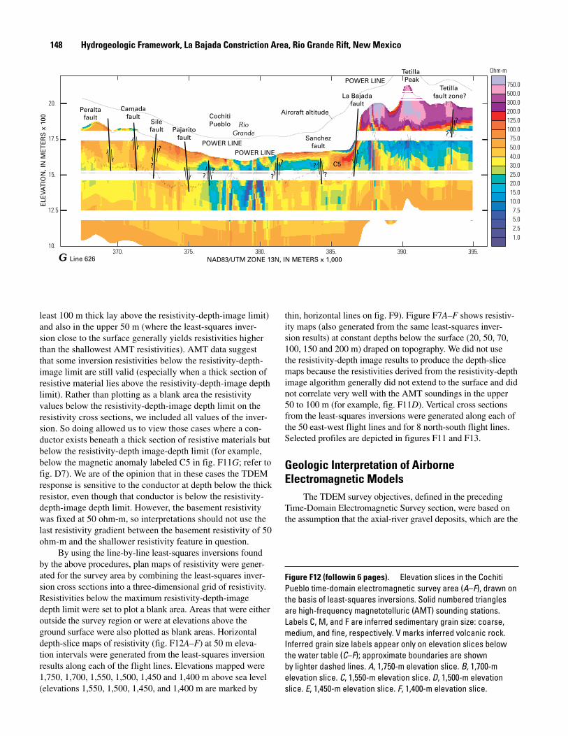
NAD83/UTM ZONE 13N, IN METERS x 1,000370. 375. 380. 385. 390. 395.
ELE
VAT
ION
, IN
ME
TE
RS
x 1
00
10.
12.5
15.
17.5
20.
Ohm-m
1.0 2.5 5.0 7.5
10.0 15.0 20.0 25.0 30.0 40.0 50.0 75.0100.0125.0200.0300.0500.0750.0POWER LINE
POWER LINEPOWER LINE
RioGrande
Aircraft altitudePeraltafault
Camadafault
Silefault
?
?
Pajaritofault
Tetilla Peak
La Bajadafault
?
?
??
CochitiPueblo
C5??
Sanchezfault
Tetilla fault zone?
G Line 626
?
?
least 100 m thick lay above the resistivity‑depth‑image limit) and also in the upper 50 m (where the least‑squares inver‑sion close to the surface generally yields resistivities higher than the shallowest AMT resistivities). AMT data suggest that some inversion resistivities below the resistivity‑depth‑image limit are still valid (especially when a thick section of resistive material lies above the resistivity‑depth‑image depth limit). Rather than plotting as a blank area the resistivity values below the resistivity‑depth‑image depth limit on the resistivity cross sections, we included all values of the inver‑sion. So doing allowed us to view those cases where a con‑ductor exists beneath a thick section of resistive materials but below the resistivity‑depth image‑depth limit (for example, below the magnetic anomaly labeled C5 in fig. F11G; refer to fig. D7). We are of the opinion that in these cases the TDEM response is sensitive to the conductor at depth below the thick resistor, even though that conductor is below the resistivity‑depth‑image depth limit. However, the basement resistivity was fixed at 50 ohm‑m, so interpretations should not use the last resistivity gradient between the basement resistivity of 50 ohm‑m and the shallower resistivity feature in question.
By using the line‑by‑line least‑squares inversions found by the above procedures, plan maps of resistivity were gener‑ated for the survey area by combining the least‑squares inver‑sion cross sections into a three‑dimensional grid of resistivity. Resistivities below the maximum resistivity‑depth‑image depth limit were set to plot a blank area. Areas that were either outside the survey region or were at elevations above the ground surface were also plotted as blank areas. Horizontal depth‑slice maps of resistivity (fig. F12A–F) at 50 m eleva‑tion intervals were generated from the least‑squares inversion results along each of the flight lines. Elevations mapped were 1,750, 1,700, 1,550, 1,500, 1,450 and 1,400 m above sea level (elevations 1,550, 1,500, 1,450, and 1,400 m are marked by
thin, horizontal lines on fig. F9). Figure F7A–F shows resistiv‑ity maps (also generated from the same least‑squares inver‑sion results) at constant depths below the surface (20, 50, 70, 100, 150 and 200 m) draped on topography. We did not use the resistivity‑depth image results to produce the depth‑slice maps because the resistivities derived from the resistivity‑depth image algorithm generally did not extend to the surface and did not correlate very well with the AMT soundings in the upper 50 to 100 m (for example, fig. F11D). Vertical cross sections from the least‑squares inversions were generated along each of the 50 east‑west flight lines and for 8 north‑south flight lines. Selected profiles are depicted in figures F11 and F13.
Geologic Interpretation of Airborne Electromagnetic Models
The TDEM survey objectives, defined in the preceding Time‑Domain Electromagnetic Survey section, were based on the assumption that the axial‑river gravel deposits, which are the
148 Hydrogeologic Framework, La Bajada Constriction Area, Rio Grande Rift, New Mexico
Figure F12 (followin 6 pages). Elevation slices in the Cochiti Pueblo time‑domain electromagnetic survey area (A–F), drawn on the basis of least‑squares inversions. Solid numbered triangles are high‑frequency magnetotelluric (AMT) sounding stations. Labels C, M, and F are inferred sedimentary grain size: coarse, medium, and fine, respectively. V marks inferred volcanic rock. Inferred grain size labels appear only on elevation slices below the water table (C–F); approximate boundaries are shown by lighter dashed lines. A, 1,750‑m elevation slice. B, 1,700‑m elevation slice. C, 1,550‑m elevation slice. D, 1,500‑m elevation slice. E, 1,450‑m elevation slice. F, 1,400‑m elevation slice.

VV
F
1750 m elevation
3930
000
3932
000
3934
000
3936
000
3938
000
3940
000
3942
000
3944
000
3946
000
3948
000
3950
000
3952
000
366000 368000 370000 372000 374000 376000 378000 380000 382000 384000 386000 388000 390000 392000 394000 396000
L65001L65001
L64901L64901
L64801 L64801
L64701 L64701
L64601L64601
L64501L64501
L64401L64401
L64301L64301
L64201L64201
L64101L64101
L64001L64001
L63901L63901
L63801L63801
L63701
L63701
L63601L63601
L63501 L63501
L63401L63401
L63301L63301
L63201
L63201
L63101L63101
L63001
L63001
L62901
L62901
L62801
L62801
L62701L62701
L62601L62601
L62501
L62501
L62401
L62401
L62301
L62301
L62201
L62201
L62101
L62101
L62001L62001
L61901
L61901
L61801L61801
L61701
L61701
L61601
L61601
L61501
L61501
L61401
L61401
L61301
L61301
L61201
L61201
L61101
L61101
L61001L61001
L60901
L60901
L60801
L60801
L60701
L60701
L60601
L60601
L60501
L60501
L60401
L60401
L60301
L60301
L60201L60201
L60101L60101
605605
609
614
626
630
638
643643
638
630
626
614
609
6001
0160
0101
6002
0160
0201
6003
0160
0301
6004
0160
0401
6005
0160
0501
6006
01
6006
01
6007
0160
0701
6008
0160
0801
NAD83 / UTM zone 13N
0 2,000 4,000 6,000 METERS2,000
2227m
COCHITI PUEBLO
COCHITI PUEBLOC
OC
HIT
I PU
EB
LO
CO
CH
ITI P
UE
BLO
Santa Fe NF
So
uth
Pajarito
fault
Cochiti fault
CochitiLake
La Bajada fault
La Bajada fault
La Bajada fault
Sile fault
Cam
ada fault
Peralta fault
Cochiti
Sanchez fault
Sanchez fault
Sanchez fault
POWER LINE
POW
ER L
INE
POW
ER L
INE
POW
ER L
INE
POW
ER L
INE
1
6
2
4
5
3
CERROS DEL RIOVOLCANIC FIELD
Cañada de
Santa Fe
Santa
FeRiver
CochitiReservoir
Rio
Gra
nde
Rio Gran
de
San Francisco fault
Tetil
la fa
ult
Saint PetersDome block
A
1.0
2.5
5.0
7.5
10.0
15.0
20.0
25.0
30.0
40.0
50.0
75.0
100.0
125.0
200.0
300.0
500.0
750.0
Ohm-m1609m
1583m
35°30’
35°37’30”
106°22’30” 106°15’
Santa CruzSprings Tract
Blow-TW
1200 well
Solar-TWCOE
TetillaCOE
CEPO 2
C1
C2
CEPO 3(Peralta)
2BW
CEPO 1(Landfill)
3-TW
CochitiElementary
180-TW
4-TW
CochitiLake 2
DomeRoad
TentRocks
170TW
2Cochiti-TW
800'well
1
Man
cos
Shal
e
Ground-Based Electromagnetic Surveys
149

VV
1700 m elevation
3930
000
3932
000
3934
000
3936
000
3938
000
3940
000
3942
000
3944
000
3946
000
3948
000
3950
000
3952
000
366000 368000 370000 372000 374000 376000 378000 380000 382000 384000 386000 388000 390000 392000 394000 396000
L65001L65001
L64901L64901
L64801 L64801
L64701 L64701
L64601L64601
L64501L64501
L64401L64401
L64301L64301
L64201L64201
L64101L64101
L64001L64001
L63901L63901
L63801L63801
L63701
L63701
L63601L63601
L63501 L63501
L63401L63401
L63301L63301
L63201
L63201
L63101L63101
L63001
L63001
L62901
L62901
L62801
L62801
L62701L62701
L62601L62601
L62501
L62501
L62401
L62401
L62301
L62301
L62201
L62201
L62101
L62101
L62001L62001
L61901
L61901
L61801L61801
L61701
L61701
L61601
L61601
L61501
L61501
L61401
L61401
L61301
L61301
L61201
L61201
L61101
L61101
L61001L61001
L60901
L60901
L60801
L60801
L60701
L60701
L60601
L60601
L60501
L60501
L60401
L60401
L60301
L60301
L60201L60201
L60101L60101
605605
609
614
626
630
638
643643
638
630
626
614
609
6001
0160
0101
6002
0160
0201
6003
0160
0301
6004
0160
0401
6005
0160
0501
6006
01
6006
01
6007
0160
0701
6008
0160
0801
NAD83 / UTM zone 13N
0 2,000 4,000 6,000 METERS2,000
COCHITI PUEBLO
COCHITI PUEBLO
CO
CH
ITI P
UE
BLO
CO
CH
ITI P
UE
BLO
Santa Fe NF
So
uth
Pajarito
fault
Cochiti fault
CochitiLake
La Bajada fault
La Bajada fault
La Bajada fault
Sile fault
Cam
ada fault
Peralta fault
Cochiti
Sanchez fault
Sanchez fault
Sanchez fault
POWER LINE
POW
ER L
INE
POW
ER L
INE
POW
ER L
INE
POW
ER L
INE
1
6
2
4
5
3
CERROS DEL RIOVOLCANIC FIELD
Cañada de
Santa Fe
Santa
FeRiver
CochitiReservoir
Rio
Gra
nde
Rio Gran
de
San Francisco fault
Tetil
la fa
ult
Saint PetersDome block
B
1.0
2.5
5.0
7.5
10.0
15.0
20.0
25.0
30.0
40.0
50.0
75.0
100.0
125.0
200.0
300.0
500.0
750.0
Ohm-m1609m
1583m
35°30’
35°37’30”
106°22’30” 106°15’
Santa CruzSprings Tract
Blow-TW
1200 well
Solar-TWCOE
TetillaCOE
CEPO 2
C1
C2
CEPO 3(Peralta)
2BW
CEPO 1(Landfill)
3-TW
CochitiElementary
180-TW
4-TW
CochitiLake 2
DomeRoad
TentRocks
170TW
2Cochiti-TW
800'well
1
Santa Fe (?) G
roup
150
Hydrogeologic Framew
ork, La Bajada Constriction Area, Rio Grande Rift, New
Mexico

1550 m elevation
3930
000
3932
000
3934
000
3936
000
3938
000
3940
000
3942
000
3944
000
3946
000
3948
000
3950
000
3952
000
366000 368000 370000 372000 374000 376000 378000 380000 382000 384000 386000 388000 390000 392000 394000 396000
L65001L65001
L64901L64901
L64801 L64801
L64701 L64701
L64601L64601
L64501L64501
L64401L64401
L64301L64301
L64201L64201
L64101L64101
L64001L64001
L63901L63901
L63801L63801
L63701
L63701
L63601L63601
L63501 L63501
L63401L63401
L63301L63301
L63201
L63201
L63101L63101
L63001
L63001
L62901
L62901
L62801
L62801
L62701L62701
L62601L62601
L62501
L62501
L62401
L62401
L62301
L62301
L62201
L62201
L62101
L62101
L62001L62001
L61901
L61901
L61801L61801
L61701
L61701
L61601
L61601
L61501
L61501
L61401
L61401
L61301
L61301
L61201
L61201
L61101
L61101
L61001L61001
L60901
L60901
L60801
L60801
L60701
L60701
L60601
L60601
L60501
L60501
L60401
L60401
L60301
L60301
L60201L60201
L60101L60101
605605
609
614
626
630
638
643643
638
630
626
614
609
6001
0160
0101
6002
0160
0201
6003
0160
0301
6004
0160
0401
6005
0160
0501
6006
01
6006
01
6007
0160
0701
6008
0160
0801
NAD83 / UTM zone 13N
0 2,000 4,000 6,000 METERS2,000
COCHITI PUEBLO
COCHITI PUEBLOC
OC
HIT
I PU
EB
LO
CO
CH
ITI P
UE
BLO
Santa Fe NF
So
uth
Pajarito
fault
Co
chiti fau
lt
CochitiLake
La Bajad
a fault
La Bajada fault
La Bajada fault
Sile fault
Cam
ada fau
lt
Peralta fault
Cochiti Sanchez fault
Sanchez fault
Sanchez fault
POWER LINE
POW
ER L
INE
POW
ER L
INE
POW
ER L
INE
POW
ER L
INE
1
6
2
4
5
3
CERROS DEL RIOVOLCANIC FIELD
Cañada de
Santa Fe
Santa
Fe
River
CochitiReservoir
Rio
Gra
nde
Rio Gran
de
San Francisco fault
Tetil
la fa
ult
Saint PetersDome block
C
1.0
2.5
5.0
7.5
10.0
15.0
20.0
25.0
30.0
40.0
50.0
75.0
100.0
125.0
200.0
300.0
500.0
750.0
Ohm-m1609m
1583m
35°30’
35°37’30”
106°22’30” 106°15’
Santa CruzSprings Tract
Blow-TW
1200 well
Solar-TW
COETetilla
COE
C1
C2
CEPO 3(Peralta)
2BW
CEPO 1(Landfill)
3-TW
CochitiElementary
180-TW
4-TW
CochitiLake 2
DomeRoad
TentRocks
170TW
2Cochiti-TW
800'well
1
CEPO 2
POWERLINE ?
V
V
V
FF
FF
FF
FF
F
CC C
C
C
C
CCC
C
C
C
C
C
M
M
M
M
M
M
MM
M
M
M
MM
M
M
F
POWER LINE
POWER LINE
Ground-Based Electromagnetic Surveys
151

1500 m elevation
3930
000
3932
000
3934
000
3936
000
3938
000
3940
000
3942
000
3944
000
3946
000
3948
000
3950
000
3952
000
366000 368000 370000 372000 374000 376000 378000 380000 382000 384000 386000 388000 390000 392000 394000 396000
L65001L65001
L64901L64901
L64801 L64801
L64701 L64701
L64601L64601
L64501L64501
L64401L64401
L64301L64301
L64201L64201
L64101L64101
L64001L64001
L63901L63901
L63801L63801
L63701
L63701
L63601L63601
L63501 L63501
L63401L63401
L63301L63301
L63201
L63201
L63101L63101
L63001
L63001
L62901
L62901
L62801
L62801
L62701L62701
L62601L62601
L62501
L62501
L62401
L62401
L62301
L62301
L62201
L62201
L62101
L62101
L62001L62001
L61901
L61901
L61801L61801
L61701
L61701
L61601
L61601
L61501
L61501
L61401
L61401
L61301
L61301
L61201
L61201
L61101
L61101
L61001L61001
L60901
L60901
L60801
L60801
L60701
L60701
L60601
L60601
L60501
L60501
L60401
L60401
L60301
L60301
L60201L60201
L60101L60101
605605
609
614
626
630
638
643643
638
630
626
614
609
6001
0160
0101
6002
0160
0201
6003
0160
0301
6004
0160
0401
6005
0160
0501
6006
01
6006
01
6007
0160
0701
6008
0160
0801
NAD83 / UTM zone 13N
0 2,000 4,000 6,000 METERS2,000
COCHITI PUEBLO
COCHITI PUEBLO
CO
CH
ITI P
UE
BLO
CO
CH
ITI P
UE
BLO
Santa Fe NF
So
uth
Pajarito
fault
Cochiti fault
CochitiLake
La Bajad
a fault
La Bajada fault
La Bajada fault
Sile fault
Cam
ada fau
lt
Peralta fault
Cochiti Sanchez fault
Sanchez fault
Sanchez fault
POWER LINE
POW
ER L
INE
POW
ER L
INE
POW
ER L
INE
POW
ER L
INE
1
6
2
4
5
3
CERROS DEL RIOVOLCANIC FIELD
Cañada de
Santa Fe
Santa
Fe
River
CochitiReservoir
Rio
Gra
nde
Rio Gran
de
San Francisco fault
Tetil
la fa
ult
Saint PetersDome block
D
1.0
2.5
5.0
7.5
10.0
15.0
20.0
25.0
30.0
40.0
50.0
75.0
100.0
125.0
200.0
300.0
500.0
750.0
Ohm-m1609m
1583m
35°30’
35°37’30”
106°22’30” 106°15’
Blow-TW
1200 well
Solar-TW
COETetilla
COE
C1
C2
2BW
CEPO 1(Landfill)
3-TWCochiti
Elementary
180-TW
4-TW
CochitiLake 2
DomeRoad
TentRocks
170TW
2Cochiti-TW
800'well
1
CEPO 2
Santa CruzSprings Tract
POWERLINE ?
POWER LINE
POWER LINE
C C C
C
C
C
C
CC
F
F
F
F
M
M
M
MM
MM
MM
M
M
M
M
M
M
M
F
F
F
F
V
V
V
V
CEPO 3(Peralta)
152
Hydrogeologic Framew
ork, La Bajada Constriction Area, Rio Grande Rift, New
Mexico

1450 m elevation
3930
000
3932
000
3934
000
3936
000
3938
000
3940
000
3942
000
3944
000
3946
000
3948
000
3950
000
3952
000
366000 368000 370000 372000 374000 376000 378000 380000 382000 384000 386000 388000 390000 392000 394000 396000
L65001L65001
L64901L64901
L64801 L64801
L64701 L64701
L64601L64601
L64501L64501
L64401L64401
L64301L64301
L64201L64201
L64101L64101
L64001L64001
L63901L63901
L63801L63801
L63701
L63701
L63601L63601
L63501 L63501
L63401L63401
L63301L63301
L63201
L63201
L63101L63101
L63001
L63001
L62901
L62901
L62801
L62801
L62701L62701
L62601L62601
L62501
L62501
L62401
L62401
L62301
L62301
L62201
L62201
L62101
L62101
L62001L62001
L61901
L61901
L61801L61801
L61701
L61701
L61601
L61601
L61501
L61501
L61401
L61401
L61301
L61301
L61201
L61201
L61101
L61101
L61001L61001
L60901
L60901
L60801
L60801
L60701
L60701
L60601
L60601
L60501
L60501
L60401
L60401
L60301
L60301
L60201L60201
L60101L60101
605605
609
614
626
630
638
643643
638
630
626
614
609
6001
0160
0101
6002
0160
0201
6003
0160
0301
6004
0160
0401
6005
0160
0501
6006
01
6006
01
6007
0160
0701
6008
0160
0801
NAD83 / UTM zone 13N
0 2,000 4,000 6,000 METERS2,000
COCHITI PUEBLO
COCHITI PUEBLOC
OC
HIT
I PU
EB
LO
CO
CH
ITI P
UE
BLO
Santa Fe NF
So
uth
Pajarito
fault
Cochiti fault
CochitiLake
La Bajad
a fault
La Bajada fault
La Bajada fault
Sile fault
Cam
ada fau
lt
Peralta fault
Cochiti Sanchez fault
Sanchez fault
Sanchez fault
POWER LINE
POW
ER L
INE
POW
ER L
INE
POW
ER L
INE
POW
ER L
INE
1
6
2
4
5
3
CERROS DEL RIOVOLCANIC FIELD
Cañada de
Santa Fe
Santa
Fe
River
CochitiReservoir
Rio
Gra
nde
Rio Gran
de
San Francisco fault
Tetil
la fa
ult
Saint PetersDome block
E
1.0
2.5
5.0
7.5
10.0
15.0
20.0
25.0
30.0
40.0
50.0
75.0
100.0
125.0
200.0
300.0
500.0
750.0
Ohm-m1609m
1583m
35°30’
35°37’30”
106°22’30” 106°15’
Blow-TW
1200 well
Solar-TW
COETetilla
COE
C1
C2
2BW
CEPO 1(Landfill)
3-TWCochiti
Elementary
180-TW
4-TW
CochitiLake 2
DomeRoad
TentRocks
170TW
2Cochiti-TW
800'well
1
POWER LINE ?
POWER LINE
POWER LINE
CEPO 2
CEPO 3(Peralta)
Santa CruzSprings Tract
M
M
M
M
M
M
M
M
M
M
F
F
F
F
FF
C
C
C
C
C
C
C
C
V
V
V
VV
Ground-Based Electromagnetic Surveys
153

M
MM
M
M
M
M
F
F
FF
C
C
C
CC
C
C
C
V
VV
1400 m elevation
3930
000
3932
000
3934
000
3936
000
3938
000
3940
000
3942
000
3944
000
3946
000
3948
000
3950
000
3952
000
366000 368000 370000 372000 374000 376000 378000 380000 382000 384000 386000 388000 390000 392000 394000 396000
L65001L65001
L64901L64901
L64801 L64801
L64701 L64701
L64601L64601
L64501L64501
L64401L64401
L64301L64301
L64201L64201
L64101L64101
L64001L64001
L63901L63901
L63801L63801
L63701
L63701
L63601L63601
L63501 L63501
L63401L63401
L63301L63301
L63201
L63201
L63101L63101
L63001
L63001
L62901
L62901
L62801
L62801
L62701L62701
L62601L62601
L62501
L62501
L62401
L62401
L62301
L62301
L62201
L62201
L62101
L62101
L62001L62001
L61901
L61901
L61801L61801
L61701
L61701
L61601
L61601
L61501
L61501
L61401
L61401
L61301
L61301
L61201
L61201
L61101
L61101
L61001L61001
L60901
L60901
L60801
L60801
L60701
L60701
L60601
L60601
L60501
L60501
L60401
L60401
L60301
L60301
L60201L60201
L60101L60101
605605
609
614
626
630
638
643643
638
630
626
614
609
6001
0160
0101
6002
0160
0201
6003
0160
0301
6004
0160
0401
6005
0160
0501
6006
01
6006
01
6007
0160
0701
6008
0160
0801
NAD83 / UTM zone 13N
0 2,000 4,000 6,000 METERS2,000
COCHITI PUEBLO
COCHITI PUEBLO
CO
CH
ITI P
UE
BLO
CO
CH
ITI P
UE
BLO
Santa Fe NF
So
uth
Pajarito
fault
Cochiti fault
CochitiLake
La Bajad
a fault
La Bajada fault
La Bajada fault
Sile fault
Cam
ada fau
lt
Peralta fault
Cochiti Sanchez fault
Sanchez fault
Sanchez fault
POWER LINE
POW
ER L
INE
POW
ER L
INE
POW
ER L
INE
POW
ER L
INE
1
6
2
4
5
3
CERROS DEL RIOVOLCANIC FIELD
Cañada de
Santa Fe
Santa
Fe
River
CochitiReservoir
Rio
Gra
nde
Rio Gran
de
Tetil
la fa
ult
Saint PetersDome block
F
1.0
2.5
5.0
7.5
10.0
15.0
20.0
25.0
30.0
40.0
50.0
75.0
100.0
125.0
200.0
300.0
500.0
750.0
Ohm-m1609m
1583m
35°30’
35°37’30”
106°22’30” 106°15’
Blow-TW
1200 well
Solar-TW
COETetilla
COE
C1
C2
2BW
CEPO 1(Landfill)
3-TW
CochitiElementary
180-TW
4-TW
CochitiLake 2
DomeRoad
TentRocks
170TW
2
Cochiti-TW
800'well
1
San Francisco
fault
CEPO 2
CEPO 3(Peralta)
Santa CruzSprings Tract
POWER LINE
POWER LINE
154
Hydrogeologic Framew
ork, La Bajada Constriction Area, Rio Grande Rift, New
Mexico

main aquifers in the middle Rio Grande Basin (Bartolino, 1999), will have a higher electrical resistivity than surrounding finer grained materials (Hearst, Nelson, and Paillet, 2000). However, the resistivities obtained from TDEM are only indirectly related to the water content and the sediment grain size at depth, and they must be correlated with other geologic information.
The correlation of TDEM inversion resistivities with grain size within the Santa Fe Group sediments was possible with the help of induction and lithologic logs from wells in the survey area. To make the correlation reliable, the well had to meet three criteria: be within 200 m of the nearest flight line, have both induction and lithologic logs in the same depth range as the TDEM survey, and be at least 200 m away from cultural noise (using a cutoff value of 10,000 microvolts) owing to power lines, pipelines, or other man‑made electrical power sources. Only four logged wells lay within areas covered by airborne surveys (Deszcz‑Pan and others, 2000) met criteria for reliability. Three wells are in Rio Rancho (survey area A+B, fig. F1); one well (CEPO 2, fig. F2A; induction log, fig. F8B) was in Cochiti Pueblo (sur‑vey area D, fig. F1). Deszcz‑Pan and others (2000) showed that one‑dimensional inversion algorithms, developed and owned by BHP World Minerals, provided resistivity cross sections that closely correlate with the Rio Rancho well logs. The resistivity inversion also closely correlates with the one Cochiti Pueblo well log (CEPO 2, fig. F2A) below the static water level (SWL, fig. F8B). Above the static water level (upper 37 m (120 ft)), the inversion resistivity under‑estimated the induction log resistivity. The underestimation probably reflects the influence of an adjacent shallow con‑ductor (20 ohm‑m) just south of CEPO 2 (fig. F7A) that dips underneath CEPO 2 at 50 m (165 ft) depth (fig. F7B). Also, at 84–102 m (275–335 ft) depth, the inversion did not resolve the interval, 9–12 m (30–40 ft) thick, of moderately resis‑tive coarse‑grained sediments (60 ohm‑m) (fig. F8B). This failure indicates that TDEM inversion for this survey was able to resolve only those resistive units whose thickness is greater than about 15 percent of their burial depth. Except for this resolution limitation and the underestimated resistivity in the upper 37 m (120 ft), the inversion correlates well with lithologic grain size below the water table.
Resistivities were correlated with grain size only in the saturated zone (Deszcz‑Pan and others, 2000), owing to the lack of information about partial saturation in the vadose zone. Deszcz‑Pan and others (2000) correlated resistivity and grain size in the saturated zone as follows: coarse grain size (40–70 ohm‑m), medium grain size (20–40 ohm‑m), and fine grain size (10–20 ohm‑m). We also observed changes in TDEM response at several faults mapped at the surface (figs. F7, F12) and at faults inferred from a high‑resolution airborne magnetic survey (Grauch, 1999; chapter D, this volume), delineating pronounced changes in lithology in Santa Fe Group sediments owing to fault juxtapositions. Variations in the pattern of resistivity can thus be linked to hydrostratigraphic changes across faults, including growth‑fault‑related facies variations in sediments of the Santa Fe Group and contemporaneous volcanic deposits.
The resistivity models obtained by the airborne TDEM survey correlate with the three principal geologic terranes in the La Bajada constriction area depicted in figure A4. Basaltic rocks of the Cerros del Rio volcanic field, in the footwall of the La Bajada fault zone (fig. F7), are characterized by very high resistivities (>500–750 ohm‑m). Higher resistivity areas generally correspond with vent areas of individual volcanoes. The tapering edges of unsaturated thin basalts generally have resistivities of 30–100 ohm‑m. The southern boundary of the resistive basalts dips north and is bounded by conductive sedimentary rocks. However, the increase in thickness of the >100 ohm‑m resistive section (fig. F14A) correlates with higher elevation cones and vents within the Cerros del Rio volcanic field. Comparison of the thickness diagram with a map of the calculated base of the resistive section (fig. F14B) clearly shows that most of the thickening pattern is due to increasing constructional topography of the Cerros del Rio volcanoes. As determined by results from AMT station 5 and the 1200‑Foot well (fig. F4B), both the volcanic lavas and the Santa Fe Group sediments thicken to the north (see also geologic cross sec‑tions, pl. 6). The east‑dipping Mancos Shale is distinctive in the depth slices at 70 and 100 ohm‑m (fig. F7C, D) just east of the Tetilla fault zone, where resistivity for this very conductive marine shale is below 7.5 ohm‑m. The east‑dipping Mancos Shale can also be seen in cross section in the 643 TDEM resis‑tivity profile (fig. F11F) east of the Tetilla fault zone. On the TDEM 1,750‑m elevation‑slice map (fig. F12A), south of the northeast‑trending power line and south of flight line 638, the Tetilla fault zone appears to form the western boundary of the east‑dipping conductive Mancos Shale. The resistivity charac‑ter of the Cerros del Rio area north of the two northeast‑ trending power lines, near AMT station 4, appears to differ from that south of the power lines. North of the power lines, the east‑dipping conductive material on the 630 TDEM resistiv‑ity profile (fig. F11D) is gone, and minor breaks disrupt what otherwise appear to be fairly flat‑lying conductive layers. The 1,700‑m‑elevation TDEM slice map (fig. F12B) depicts mod‑erately resistive material surrounded by moderately conduc‑tive material, which suggests a structural block between AMT stations 4 and 5 at a bearing of about N. 60° E. The structure of this block can also be seen north of AMT station 4 in the north‑south 600701 TDEM resistivity profile (fig. F13G) and south of AMT station 5 in the north‑south 600801 TDEM resis‑tivity profile (fig. F13H). The moderately resistive character of this section is similar to that of sediments in the Santa Fe Group.
The western terrane, Saint Peters Dome block (figs. F12, F7), also displays high resistivity values in the footwall block of the Pajarito fault zone, and those higher resistivities con‑tinue south into the Santo Domingo Basin between the Pajarito and Sile faults. In the west, an exposed rhyolite dome and related pyroclastic deposits near Tent Rocks (V, figs. F12, F7) have high resistivities. The dome and pyroclastic deposits have peak resistivities greater than 500–750 ohm‑m in the depth range of 100–150 m below the surface, so their highest values are more limited here than in the basaltic rocks of the Cerros
Ground-Based Electromagnetic Surveys 155

Sile fault6
300
10
30
100
3930. 3935. 3940. 3945. 3950.
ELE
VAT
ION
, IN
ME
TE
RS
x 1
00
10.
12.5
15.
17.5
20.
Ohm-m
1.0 2.5 5.0 7.5
10.0 15.0 20.0 25.0 30.0 40.0 50.0 75.0100.0125.0200.0300.0500.0750.0
Line 600201 NAD83/UTM ZONE 13N, IN METERS x 1,000
B
Peraltafault zone
1
100
10
30
? ?
3930. 3935. 3940. 3945. 3950.
ELE
VAT
ION
, IN
ME
TE
RS
x 1
00
10.
12.5
15.
17.5
20.
Ohm-m
1.0 2.5 5.0 7.5
10.0 15.0 20.0 25.0 30.0 40.0 50.0 75.0100.0125.0200.0300.0500.0750.0
Line 600101 NAD83/UTM ZONE 13N, IN METERS x 1,000
A
156 Hydrogeologic Framework, La Bajada Constriction Area, Rio Grande Rift, New Mexico
Figure F13 (below and following 2 pages). North‑south profiles in the Cochiti Pueblo time‑domain electromagnetic survey area (cross sections A–H), drawn on the basis of least‑squares inversions. Dashed line in each section is maximum depth estimated from resistivity‑depth image; numbers below wells or stations represent modeled resistivities. Vertical exaggeration is 10. A, Flight line 600101 showing audiomagnetotelluric (AMT) station 1. B, Flight line 600201 showing AMT station 6. C, Flight line 600301 showing Dome Road well. D, Flight line 600401 showing Sanchez fault. E, Flight line 600501 showing La Bajada fault zone. F, Flight line 600601 showing La Bajada fault zone. G, Flight line 600701 showing AMT station 4. H, Flight line 600801 showing AMT station 5 and 1200‑Foot well.

Dome Road
Power line
SouthPajarito
fault
3930. 3935. 3940. 3945. 3950.
ELE
VAT
ION
, IN
ME
TE
RS
x 1
00
10.
12.5
15.
17.5
20.
Ohm-m
1.0 2.5 5.0 7.5
10.0 15.0 20.0 25.0 30.0 40.0 50.0 75.0100.0125.0200.0300.0500.0750.0
Line 600301 NAD83/UTM ZONE 13N, IN METERS x 1,000
C
POWER LINE
Sanchezfault
3930. 3935. 3940. 3945. 3950.
ELE
VAT
ION
, IN
ME
TE
RS
x 1
00
10.
12.5
15.
17.5
20.
Ohm-m
1.0 2.5 5.0 7.5
10.0 15.0 20.0 25.0 30.0 40.0 50.0 75.0100.0125.0200.0300.0500.0750.0
Line 600401 NAD83/UTM ZONE 13N, IN METERS x 1,000
D
3930. 3935. 3940. 3945. 3950.
ELE
VAT
ION
, IN
ME
TE
RS
x 1
00
10.
12.5
15.
17.5
20.
Ohm-m
1.0 2.5 5.0 7.5
10.0 15.0 20.0 25.0 30.0 40.0 50.0 75.0100.0125.0200.0300.0500.0750.0
Line 600501 NAD83/UTM ZONE 13N, IN METERS x 1,000
E
POWER LINE Santa FeRiver
La Bajadafault
Ground-Based Electromagnetic Surveys 157

POWER LINES
POWER LINESCañada deSanta Fe
Tetilla Peak
5
Tetilla fault ?
Moderatelyconductive
material
4
100
2
10300
3930. 3935. 3940. 3945. 3950.
ELE
VAT
ION
, IN
ME
TE
RS
x 1
00
10.
12.5
15.
17.5
20.
Ohm-m
1.0 2.5 5.0 7.5
10.0 15.0 20.0 25.0 30.0 40.0 50.0 75.0100.0125.0200.0300.0500.0750.0
Line 600701 NAD83/UTM ZONE 13N, IN METERS x 1,000
G
POWER LINE
Cañada de Santa Fe 1200-Foot 5
100
10030
1000
3930. 3935. 3940. 3945. 3950.
ELE
VAT
ION
, IN
ME
TE
RS
x 1
00
10.
12.5
15.
17.5
20.
Ohm-m
1.0 2.5 5.0 7.5
10.0 15.0 20.0 25.0 30.0 40.0 50.0 75.0100.0125.0200.0300.0500.0750.0
Line 600801 NAD83/UTM ZONE 13N, IN METERS x 1,000
H
158 Hydrogeologic Framework, La Bajada Constriction Area, Rio Grande Rift, New Mexico
POWER LINE
POWER LINE
La Bajadafault
Cerro Colorado
3930. 3935. 3940. 3945. 3950.
ELE
VAT
ION
, IN
ME
TE
RS
x 1
00
10.
12.5
15.
17.5
20.
Ohm-m
1.0 2.5 5.0 7.5
10.0 15.0 20.0 25.0 30.0 40.0 50.0 75.0100.0125.0200.0300.0500.0750.0
Line 600601 NAD83/UTM ZONE 13N, IN METERS x 1,000
F

del Rio volcanic field. Resistivity values in the adjoining Cochiti Formation volcaniclastic sediments and axial gravels are also moderately high, in the range of 40–200 ohm‑m.
The central La Bajada constriction area (that is, within the Santo Domingo Valley, fig. A4) has the lowest resistivi‑ties overall, and deposits in this area are generally less than 50 ohm‑m resistivity. In the northern part of this area, a large area of lower resistivity coincides with a silt or clay lacustrine unit (F, near station AMT–2, figs. F12, F7) concealed within deposits of the upper Santa Fe Group. In the central part of the map area, higher resistivities correspond in part with ances‑tral Rio Grande axial‑gravel deposits (C, M, fig. F12C–F). In areas lacking other subsurface information, boundaries within these deposits were inferred on the basis of grain size (fig. F12C–F); grain size, in turn, was established primarily on the basis of resistivity calibration (as previously described), but it was also constrained by local AMT soundings and lithologic well logs (Deszcz‑Pan and others, 2000). The AMT sound‑ings also helped us interpret the northern part of the survey area where thin (30–50 m) but strongly conductive, clay‑rich sediments (<10 ohm‑m) or rocks effectively blocked out those portions of the elevation‑slice maps (fig. F12C–F) derived from the TDEM resistivity inversions. The TDEM data west of the La Bajada fault zone show that relatively lower resistivity values correspond with Santa Fe Group piedmont alluvium deposits, whereas relatively higher resistivity values correspond with axial gravel deposits of the ancestral Rio Grande. A large region of buried volcanic rock (V, fig. F12) in the subsurface of the Santo Domingo Basin is imaged by the modeled TDEM data. For example, aeromagnetic data (chapter D, this volume) indicate that a basaltic vent is buried just to the west of the Sanchez fault (magnetic anomaly C3, figs. F7, F11D), that abundant volcanic clasts contribute to the moderate resistivities just west of the Santa Cruz Springs well (magnetic anomaly C4, figs. F7, F11D), and that the rhyolite at the core of the W4 magnetic high (figs. F7, F11B) is at least 250 m thick and has resistivities well above 200 ohm‑m. The apparent reduction in spatial size of the displayed resistivities for the deeper elevation slices (fig. F12D–F) is in part due to the depth‑of‑penetration limits of the TDEM survey. More detailed geologic interpretation and comparison of features seen in the TDEM models with geology and other geophysical data sets are discussed in chapter G (this volume).
SummaryTime‑domain electromagnetic and magnetotelluric data
were used to map changes in electrical resistivity with depth; these changes in resistivity are related to variations in rock types at depth; these variations in turn influence aquifers in the study area. These aquifers are part of the groundwater system hydraulically connected with the Rio Grande as it passes from the Española Basin into the Santo Domingo Basin.
In the area of the eastern Cerros del Rio volcanic field, the northern boundary of the Cerrillos uplift is con‑
1.
strained by magnetotelluric data reported in this chapter. Magnetotelluric soundings (figs. F4, F5) indicate that along a north‑south line between audio‑magnetotelluric stations 4 and 5, a 2 ohm‑m conductor inferred to be the Cretaceous Mancos Shale is downdropped from a depth of 180 m at audio‑magnetotelluric station 4 to a depth of 1,150 m beneath the surface at audio‑magnetotelluric station This offset is evidence for 800 m of Tertiary structural relief at the north end of the Cerrillos uplift. The shallow Mancos Shale located at audio‑magnetotelluric station 4, immedi‑ately south of Tetilla Peak, provides the farthest northwest constraint for the edge of the Cerrillos uplift and is consis‑tent with the subsurface extent of the uplift based on gravity data.
Also in the area of the eastern Cerros del Rio volcanic field, the partly concealed Tetilla fault zone appears to form the western boundary of the east‑dipping conductive Mancos Shale, based on time‑domain electromagnetic results south of two northeast‑trending power lines (fig. F11F). We do not see the same east‑dipping conductive material in the terrane north of the power lines, near audio‑magnetotelluric station 4 (fig. F11D), but rather we see minor breaks in what otherwise look like fairly flat‑lying conductive layers. Moderately resistive material surrounded by moderately conductive material suggests some kind of structural block between audiomagnetotelluric stations 4 and 5 at a bearing of about N. 60° E. (fig. F12B). The structure of this block can also be seen north of audiomagnetotelluric station 4 (fig. F13G) and south of audiomagnetotelluric station 5 (fig. F13H). This moderately resistive block has resistivities similar to those of Santa Fe Group sediments.
In the northern part of the central La Bajada constriction, a large area of lower resistivity, defined by the time‑domain electromagnetic survey results, coincides with a silt or clay lacustrine unit (region F, near audiomag‑netotelluric station 2, figs. F12, F7) in the upper Santa Fe Group deposits. In the central part of the map, higher resistivities correspond in part with ancestral Rio Grande axial‑gravel deposits (regions C and M, fig. F12).
The Saint Peters Dome block, in the footwall of the Pajarito fault zone, has a more complex stratigraphy than expected on the basis of the magnetotelluric results. Magnetotelluric soundings (fig. F6, magnetotelluric stations 12 and 17) pro‑vide additional constraints on the relative position of base‑ment and thickness of Paleozoic, Mesozoic, and Tertiary sedimentary rocks across the Pajarito fault zone.
2.
3.
4.
Ground-Based Electromagnetic Surveys 159
Figure F14 (following 2 pages). A, Depth to surface of resistive layer (>100 ohm‑m) in the Cochiti Pueblo time‑domain electromagnetic survey area, drawn on the basis of least‑squares inversion. B, Elevation to base of surface resistive layer (>100 ohm‑m) in the Cochiti Pueblo time‑domain electromagnetic survey area, drawn on the basis of least‑squares inversion.

COCHITI PUEBLO
CO
CH
ITI P
UE
BLO
Santa Fe NF
South Pajarito fault
Cochiti fault
COCHITILAKE
Tetilla Peak
La Bajad
a fault
La Bajada fault
La Bajada fault
Sile fault
Cam
ada fau
lt
Peralta fault
CochitiPueblo
Santa Fe
Cañada De
POWER L
INE
POW
ER L
INE
AMT-1AMT-6
AMT-2
AMT-4
AMT-5
AMT-3
370 375 380 385 390 395106°15’106°22’30”
106°22’30”
35°3
7’30
”35
°30’
3945
3950
3940
3935
3930
2227m
COCHITIRESERVOIR
Rio Grande
Pe–a blancabasalt
Santa FeR
iver
CerroColorado
CERROS DEL RIOVOLCANIC FIELD
Rio
Gra
nde
106°15'1609m
1583m
Santa CruzSprings tract
Blow-TW
1200 well
Solar-TW
COETetilla
COE
CEPO2
C1
C2
CEPO3(Peralta)
2BW
CEPO1(Landfill)3-TW
CochitiElementary
180-TW
4-TW
CochitiLake 2
DomeRoad
170TW
2
Cochiti-TW
800' well
1
NAD27/UTM ZONE 13N
0 3 6 KILOMETERS
200250300
150100502510
Depth to100 ohm-m boundary
A 160
Hydrogeologic Framew
ork, La Bajada Constriction Area, Rio Grande Rift, New
Mexico

COCHITI PUEBLO
CO
CH
ITI P
UE
BLO
Santa Fe NF
South Pajarito fault
Cochiti fault
COCHITILAKE
Tetilla PeakLa B
ajada fau
lt
La Bajada fault
La Bajada fault
Sile fault
Cam
ada fau
lt
Peralta fault
CochitiPueblo
Santa Fe
Cañada De
POWER L
INE
POW
ER L
INE
AMT-1AMT-6
AMT-2
AMT-4
AMT-5
AMT-3
370 375 380 385 390 395106°15’106°22’30”
106°22’30”
35°3
7’30
”35
°30’
3945
3950
3940
3935
3930
2227m
COCHITIRESERVOIR
Rio Grande
Pe–a blancabasalt
Santa FeR
iver
CerroColorado
CERROS DEL RIOVOLCANIC FIELD
Rio
Gra
nde
106°15'1609m
1583m
Santa CruzSprings tract
Blow-TW
1200 well
Solar-TW
COETetilla
COE
CEPO2
C1
C2
CEPO3(Peralta)
2BW
CEPO1(Landfill)3-TW
CochitiElementary
180-TW
4-TW
CochitiLake 2
DomeRoad
170TW
2
Cochiti-TW
800' well
1
NAD27/UTM ZONE 13N
0 3 6 KILOMETERS
Depth in m of100 ohm-m boundary
15831596161616291645166016621671167916871697170917241740175717761798181918381851186418761888190219201938195719761996201220262039205420712090212021662250
BGround-Based Electrom
agnetic Surveys
161

References Cited
Bartolino, J.R., 1999, Introduction, in U.S. Geological Survey Middle Rio Grande Basin Study— 3d Annual Work‑shop, Albuquerque, New Mexico, February 24–25, 1999, Proceedings: U.S. Geological Survey Open‑File Report 99–203, p. 2.
Bartolino, J.R., and Cole, J.C., 2002, Ground‑water resources of the Middle Rio Grande Basin, New Mexico: U.S. Geo‑logical Survey Circular 1222, 132 p.
Bendat, J.S., and Piersol, A.G., 1971, Random data—Analysis and measurement procedures: New York, Wiley Interscience, 407 p.
Chamberlin, R.M., Jackson, P., and Connell, S.D., 1999, Field logs of borehole drilled for monitoring well at Dome Road site, Canada de Cochiti Grant, Sandoval County, New Mex‑ico: New Mexico Bureau of Mines and Mineral Resources Open‑file Report 444c, 30 p.
Clarke, J., Gamble, T.D., Goubau, W.M., Koch, R.H., and Miracky, R.F., 1983, Remote‑reference magnetotellurics—Equipment and procedures: Geophysical Prospecting, v. 31, p. 149–170.
Cole, J.C., Grauch, V.J.S., Hudson, M.R., Maldonado, F., Minor, S.A., Sawyer, D.A., and Stone, B.D., 1999, Three‑ dimensional geologic modeling of the middle Rio Grande Basin, in Bartolino, J.R., ed., U.S. Geological Survey Middle Rio Grande Basin Study—3d Annual Workshop, Albuquer‑que, New Mexico, February 24–25, 1999, Proceedings: U.S. Geological Survey Open‑File Report 99–203, p. 25–26.
Deszcz‑Pan, M., Rodriguez, B.D., Doucette, J.P., Godbout, M., Williams, J.M., Sawyer, D.A., Stone, B.D., and Grauch, V.J.S., 2000, Digital airborne time domain electromagnetic data from surveys over Cochiti Pueblo, Rio Puerco, and Rio Rancho, New Mexico: U.S. Geological Survey Open‑File Report 00–502 (CD‑ROM).
Dobrin, M.D., and Savit, C.H., 1988, Introduction to geophys‑ical prospecting (4th ed.): New York, McGraw‑Hill, 867 p.
Ellis, R.G., 1998, Inversion of airborne electromagnetic data: Exploration Geophysics, v. 29, no. 1–2, p. 121–127.
Gamble, T.D., Goubau, W.M., and Clarke, J., 1979, Magneto‑tellurics with a remote magnetic reference: Geophysics, v. 44, no. 1, p. 53–68.
Grauch, V.J.S., 1999, Principal features of high‑resolution aeromagnetic data collected near Albuquerque, New Mex‑ico: New Mexico Geological Society 50th field conference, Albuquerque Geology, Guidebook, p. 115–118, 133–135.
Hearst, J.R., Nelson, P.H., and Paillet, F.L., 2000, Well logging for physical properties, 2d ed.: New York, John Wiley, 483 p.
Keller, G.V., 1987, Rock and mineral properties, in Nabighian, M.N., ed., Electromagnetic methods in applied geophysics, v. 1, Theory: Society of Exploration Geophysicists, p. 13–51.
Keller, G.V., and Frischknecht, F.C., 1966, Electrical methods in geophysical prospecting: New York, Pergamon Press, 517 p.
Liu, G., and Asten, M.A., 1993, Conductance‑depth imaging of airborne TEM data: Exploration Geophysics, v. 24, no. 3–4, p. 655–662.
Nelson, P.H., and Anderson, L.A., 1992, Physical properties of ash flow tuff from Yucca Mountain, Nevada: Journal of Geophysical Research, v. 97, no. B5, p. 6823–6841.
Palacky, G.J., 1987, Resistivity characteristics of geologic targets, in Nabighian, M.N., ed., Electromagnetic methods in applied geophysics, v. 1, Theory: Society of Exploration Geophysicists, p. 53–129.
Palacky, G.J., and West, G.F., 1991, Airborne electromagnetic methods, in Nabighian, M.N., ed., Electromagnetic methods in applied geophysics, v. 2, Application: Society of Explora‑tion Geophysicists, p. 811–879.
Smith, G.A., 2001, Development of a pyroclastic apron adja‑cent to rhyolite domes in a subsiding basin, upper Miocene Peralta Tuff, Jemez Mountains, New Mexico: New Mexico Museum of Natural History and Science, v. 18, p. 85–96.
Sternberg, B.K., Washburne, J.C., and Pellerin, L., 1988, Correction for the static shift in magnetotellurics using transient electromagnetic soundings: Geophysics, v. 53, p. 1459–1468.
Vozoff, K., 1972, The magnetotelluric method in the explora‑tion of sedimentary basins: Geophysics, v. 37, p. 98–141.
Vozoff, K., 1991, The magnetotelluric method, in Nabighian, M.N., ed., Electromagnetic methods in applied geophysics, v. 2, Application, part B: Society of Exploration Geophysi‑cists, Tulsa, Oklahoma, p. 641–711.
Wannamaker, P.E., Hohmann, G.W., and Ward, S.H., 1984, Magnetotelluric responses of three‑dimensional bodies in layered earths: Geophysics, v. 49, no. 9, p. 1517–1533.
Wannamaker, P.E., Stodt, J.A., and Rijo, L., 1985, PW2D—Finite element program for solution of magnetotelluric responses of two‑dimensional earth resistivity structure (user documentation): Salt Lake City, Utah, Earth Science Laboratory, University of Utah Research Institute, 40 p.
Williams, J.M., and Rodriguez, B.D., 2003, Magnetotelluric data in the southwest Española Basin, northern New Mexico: U.S. Geological Survey Open‑File Report 03–199, 128 p.
Williams, J.M., Rodriguez, B.D., and Sampson, J.A., 2001, Magnetotelluric data in the Cochiti Pueblo area, New Mex‑ico: U.S. Geological Survey Open‑File Report 01–442, 66 p.
162 Hydrogeologic Framework, La Bajada Constriction Area, Rio Grande Rift, New Mexico

Ground-Based Electromagnetic Surveys 163
Published in the Central Region, Denver, Colo.Manuscript approved for publication February 10, 2006Graphics by authorsPhotocomposition by Mari L. Kauffmann (Contractor, ATA Services)Edited by Mary‑Margaret Coates (Contractor, ATA Services)