electromagnetism and optics - · pdf fileelectromagnetism and optics an introductory course...
TRANSCRIPT

Electromagnetism and OpticsAn introductory course
Richard Fitzpatrick
Professor of Physics
The University of Texas at Austin

Contents
1 Introduction 8
2 Vectors 9
2.1 Vector Algebra . . . . . . . . . . . . . . . . . . . . . . . . . . . . . . . . . . . . . . 9
2.2 Vector Area . . . . . . . . . . . . . . . . . . . . . . . . . . . . . . . . . . . . . . . . 12
2.3 The Scalar Product . . . . . . . . . . . . . . . . . . . . . . . . . . . . . . . . . . . . 14
2.4 The Vector Product . . . . . . . . . . . . . . . . . . . . . . . . . . . . . . . . . . . . 16
2.5 Vector Calculus . . . . . . . . . . . . . . . . . . . . . . . . . . . . . . . . . . . . . . 19
2.6 Line Integrals . . . . . . . . . . . . . . . . . . . . . . . . . . . . . . . . . . . . . . . 20
2.7 Surface Integrals . . . . . . . . . . . . . . . . . . . . . . . . . . . . . . . . . . . . . 21
2.8 Volume Integrals . . . . . . . . . . . . . . . . . . . . . . . . . . . . . . . . . . . . . 22
3 Electricity 24
3.1 Historical Introduction . . . . . . . . . . . . . . . . . . . . . . . . . . . . . . . . . . 24
3.2 Conductors and Insulators . . . . . . . . . . . . . . . . . . . . . . . . . . . . . . . . 25
3.3 Electrometers and Electroscopes . . . . . . . . . . . . . . . . . . . . . . . . . . . . . 26
3.4 Induced Electric Charge . . . . . . . . . . . . . . . . . . . . . . . . . . . . . . . . . 27
3.5 Coulomb’s Law . . . . . . . . . . . . . . . . . . . . . . . . . . . . . . . . . . . . . . 29
3.6 Electric Fields . . . . . . . . . . . . . . . . . . . . . . . . . . . . . . . . . . . . . . . 31
3.7 Worked Examples . . . . . . . . . . . . . . . . . . . . . . . . . . . . . . . . . . . . . 33
4 Gauss’ Law 37
4.1 Electric Field-Lines . . . . . . . . . . . . . . . . . . . . . . . . . . . . . . . . . . . . 37
4.2 Gauss’ Law . . . . . . . . . . . . . . . . . . . . . . . . . . . . . . . . . . . . . . . . 38
2

4.3 Electric Field of a Spherical Conducting Shell . . . . . . . . . . . . . . . . . . . . . 39
4.4 Electric Field of a Uniformly Charged Wire . . . . . . . . . . . . . . . . . . . . . . . 41
4.5 Electric Field of a Uniformly Charged Plane . . . . . . . . . . . . . . . . . . . . . . 42
4.6 Charged Conductors . . . . . . . . . . . . . . . . . . . . . . . . . . . . . . . . . . . 44
4.7 Worked Examples . . . . . . . . . . . . . . . . . . . . . . . . . . . . . . . . . . . . . 45
5 Electric Potential 46
5.1 Electric Potential Energy . . . . . . . . . . . . . . . . . . . . . . . . . . . . . . . . . 46
5.2 Electric Potential . . . . . . . . . . . . . . . . . . . . . . . . . . . . . . . . . . . . . 51
5.3 Electric Potential and Electric Field . . . . . . . . . . . . . . . . . . . . . . . . . . . 52
5.4 Electric Potential of a Point Charge . . . . . . . . . . . . . . . . . . . . . . . . . . . 56
5.5 Worked Examples . . . . . . . . . . . . . . . . . . . . . . . . . . . . . . . . . . . . . 57
6 Capacitance 63
6.1 Charge Storage . . . . . . . . . . . . . . . . . . . . . . . . . . . . . . . . . . . . . . 63
6.2 Breakdown . . . . . . . . . . . . . . . . . . . . . . . . . . . . . . . . . . . . . . . . 64
6.3 Capacitance . . . . . . . . . . . . . . . . . . . . . . . . . . . . . . . . . . . . . . . . 67
6.4 Dielectrics . . . . . . . . . . . . . . . . . . . . . . . . . . . . . . . . . . . . . . . . . 68
6.5 Capacitors in Series and in Parallel . . . . . . . . . . . . . . . . . . . . . . . . . . . 71
6.6 Energy Stored by Capacitors . . . . . . . . . . . . . . . . . . . . . . . . . . . . . . . 74
6.7 Worked Examples . . . . . . . . . . . . . . . . . . . . . . . . . . . . . . . . . . . . . 76
7 Electric Current 81
7.1 Electric Circuits . . . . . . . . . . . . . . . . . . . . . . . . . . . . . . . . . . . . . . 81
7.2 Ohm’s Law . . . . . . . . . . . . . . . . . . . . . . . . . . . . . . . . . . . . . . . . 83
7.3 Resistance and Resistivity . . . . . . . . . . . . . . . . . . . . . . . . . . . . . . . . 85
3

7.4 Emf and Internal Resistance . . . . . . . . . . . . . . . . . . . . . . . . . . . . . . . 86
7.5 Resistors in Series and in Parallel . . . . . . . . . . . . . . . . . . . . . . . . . . . . 88
7.6 Kirchhoff’s Rules . . . . . . . . . . . . . . . . . . . . . . . . . . . . . . . . . . . . . 91
7.7 Capacitors in DC Circuits . . . . . . . . . . . . . . . . . . . . . . . . . . . . . . . . . 92
7.8 Energy in DC Circuits . . . . . . . . . . . . . . . . . . . . . . . . . . . . . . . . . . . 92
7.9 Power and Internal Resistance . . . . . . . . . . . . . . . . . . . . . . . . . . . . . . 94
7.10 Worked Examples . . . . . . . . . . . . . . . . . . . . . . . . . . . . . . . . . . . . . 96
8 Magnetism 101
8.1 Historical Introduction . . . . . . . . . . . . . . . . . . . . . . . . . . . . . . . . . . 101
8.2 Ampere’s Experiments . . . . . . . . . . . . . . . . . . . . . . . . . . . . . . . . . . 102
8.3 Ampere’s Law . . . . . . . . . . . . . . . . . . . . . . . . . . . . . . . . . . . . . . . 105
8.4 The Lorentz Force . . . . . . . . . . . . . . . . . . . . . . . . . . . . . . . . . . . . . 107
8.5 Charged Particle in a Magnetic Field . . . . . . . . . . . . . . . . . . . . . . . . . . 110
8.6 The Hall Effect . . . . . . . . . . . . . . . . . . . . . . . . . . . . . . . . . . . . . . 113
8.7 Ampere’s Circuital Law . . . . . . . . . . . . . . . . . . . . . . . . . . . . . . . . . . 115
8.8 Magnetic Field of a Solenoid . . . . . . . . . . . . . . . . . . . . . . . . . . . . . . . 117
8.9 Origin of Permanent Magnetism . . . . . . . . . . . . . . . . . . . . . . . . . . . . . 118
8.10 Gauss’ Law for Magnetic Fields . . . . . . . . . . . . . . . . . . . . . . . . . . . . . 122
8.11 Galvanometers . . . . . . . . . . . . . . . . . . . . . . . . . . . . . . . . . . . . . . 123
8.12 Worked Examples . . . . . . . . . . . . . . . . . . . . . . . . . . . . . . . . . . . . . 128
9 Magnetic Induction 133
9.1 Faraday’s Law . . . . . . . . . . . . . . . . . . . . . . . . . . . . . . . . . . . . . . . 133
9.2 Lenz’s Law . . . . . . . . . . . . . . . . . . . . . . . . . . . . . . . . . . . . . . . . . 135
4

9.3 Magnetic Induction . . . . . . . . . . . . . . . . . . . . . . . . . . . . . . . . . . . . 136
9.4 Motional Emf . . . . . . . . . . . . . . . . . . . . . . . . . . . . . . . . . . . . . . . 140
9.5 Eddy Currents . . . . . . . . . . . . . . . . . . . . . . . . . . . . . . . . . . . . . . . 143
9.6 The Alternating Current Generator . . . . . . . . . . . . . . . . . . . . . . . . . . . 145
9.7 The Direct Current Generator . . . . . . . . . . . . . . . . . . . . . . . . . . . . . . 149
9.8 The Alternating Current Motor . . . . . . . . . . . . . . . . . . . . . . . . . . . . . 151
9.9 The Direct Current Motor . . . . . . . . . . . . . . . . . . . . . . . . . . . . . . . . 154
9.10 Worked Examples . . . . . . . . . . . . . . . . . . . . . . . . . . . . . . . . . . . . . 157
10 Inductance 163
10.1 Mutual Inductance . . . . . . . . . . . . . . . . . . . . . . . . . . . . . . . . . . . . 163
10.2 Self Inductance . . . . . . . . . . . . . . . . . . . . . . . . . . . . . . . . . . . . . . 166
10.3 Energy Stored in an Inductor . . . . . . . . . . . . . . . . . . . . . . . . . . . . . . 167
10.4 The RL Circuit . . . . . . . . . . . . . . . . . . . . . . . . . . . . . . . . . . . . . . . 169
10.5 The RC Circuit . . . . . . . . . . . . . . . . . . . . . . . . . . . . . . . . . . . . . . 173
10.6 Transformers . . . . . . . . . . . . . . . . . . . . . . . . . . . . . . . . . . . . . . . 177
10.7 Impedance Matching . . . . . . . . . . . . . . . . . . . . . . . . . . . . . . . . . . . 182
10.8 Worked Examples . . . . . . . . . . . . . . . . . . . . . . . . . . . . . . . . . . . . . 183
11 Electromagnetic Waves 188
11.1 Maxwell’s Equations . . . . . . . . . . . . . . . . . . . . . . . . . . . . . . . . . . . 188
11.2 Electromagnetic Waves . . . . . . . . . . . . . . . . . . . . . . . . . . . . . . . . . . 193
11.3 Effect of Dielectric Materials . . . . . . . . . . . . . . . . . . . . . . . . . . . . . . . 197
11.4 Energy in Electromagnetic Waves . . . . . . . . . . . . . . . . . . . . . . . . . . . . 197
11.5 Worked Examples . . . . . . . . . . . . . . . . . . . . . . . . . . . . . . . . . . . . . 199
5

12 Geometric Optics 201
12.1 Introduction . . . . . . . . . . . . . . . . . . . . . . . . . . . . . . . . . . . . . . . . 201
12.2 History of Geometric Optics . . . . . . . . . . . . . . . . . . . . . . . . . . . . . . . 202
12.3 Law of Geometric Propagation . . . . . . . . . . . . . . . . . . . . . . . . . . . . . . 203
12.4 Law of Reflection . . . . . . . . . . . . . . . . . . . . . . . . . . . . . . . . . . . . . 206
12.5 Law of Refraction . . . . . . . . . . . . . . . . . . . . . . . . . . . . . . . . . . . . . 207
12.6 Total Internal Reflection . . . . . . . . . . . . . . . . . . . . . . . . . . . . . . . . . 210
12.7 Dispersion . . . . . . . . . . . . . . . . . . . . . . . . . . . . . . . . . . . . . . . . . 213
12.8 Rainbows . . . . . . . . . . . . . . . . . . . . . . . . . . . . . . . . . . . . . . . . . 215
12.9 Worked Examples . . . . . . . . . . . . . . . . . . . . . . . . . . . . . . . . . . . . . 219
13 Paraxial Optics 222
13.1 Spherical Mirrors . . . . . . . . . . . . . . . . . . . . . . . . . . . . . . . . . . . . . 222
13.2 Image Formation by Concave Mirrors . . . . . . . . . . . . . . . . . . . . . . . . . . 225
13.3 Image Formation by Convex Mirrors . . . . . . . . . . . . . . . . . . . . . . . . . . 230
13.4 Image Formation by Plane Mirrors . . . . . . . . . . . . . . . . . . . . . . . . . . . 233
13.5 Thin Lenses . . . . . . . . . . . . . . . . . . . . . . . . . . . . . . . . . . . . . . . . 234
13.6 Image Formation by Thin Lenses . . . . . . . . . . . . . . . . . . . . . . . . . . . . 239
13.7 Chromatic aberration . . . . . . . . . . . . . . . . . . . . . . . . . . . . . . . . . . . 244
13.8 Worked Examples . . . . . . . . . . . . . . . . . . . . . . . . . . . . . . . . . . . . . 245
14 Wave Optics 249
14.1 Introduction . . . . . . . . . . . . . . . . . . . . . . . . . . . . . . . . . . . . . . . . 249
14.2 Huygens’ principle . . . . . . . . . . . . . . . . . . . . . . . . . . . . . . . . . . . . 251
14.3 Young’s Double-Slit Experiment . . . . . . . . . . . . . . . . . . . . . . . . . . . . . 252
6

14.4 Interference in Thin Films . . . . . . . . . . . . . . . . . . . . . . . . . . . . . . . . 256
14.5 Worked Examples . . . . . . . . . . . . . . . . . . . . . . . . . . . . . . . . . . . . . 258
7

1 INTRODUCTION
1 Introduction
These lecture notes are designed to accompany a lower-division college survey
course covering electricity, magnetism, and optics. Students are expected to be
familiar with calculus and elementary mechanics.
8

2 VECTORS
2 Vectors
2.1 Vector Algebra
In applied mathematics, physical quantities are (predominately) represented by
two distinct classes of objects. Some quantities, denoted scalars, are represented
by real numbers. Others, denoted vectors, are represented by directed line ele-
ments in space: e.g.,→PQ in see Fig. 2.1. Note that line elements (and, therefore,
vectors) are movable, and do not carry intrinsic position information: i.e., in
Fig. 2.2,→PS and
→QR are considered to be the same vector. In fact, vectors just
possess a magnitude and a direction, whereas scalars possess a magnitude but no
direction. By convention, vector quantities are denoted by bold-faced characters
(e.g., a) in typeset documents. Vector addition can be represented using a par-
allelogram: e.g.,→PR=
→PQ +
→QR in Fig. 2.2.
→PR is said to be the resultant of
→PQ
and→QR. Suppose that a ≡
→PQ≡
→SR, b ≡
→QR≡
→PS, and c ≡
→PR. It follows, from
Fig. 2.2, that vector addition is commutative: i.e., a + b = b + a (since→PR is also
the resultant of→PS and
→SR). It can also be shown that the associative law holds:
i.e., a + (b + c) = (a + b) + c.
There are two general approaches to vector analysis. The geometric approach
is based on drawing line elements in space, and then making use of the theorems
of Euclidian geometry. The coordinate approach assumes that space is defined
by Cartesian coordinates, and uses these to characterize vectors. In Physics, we
P
Q
Figure 2.1: A directed line element.
9

2 VECTORS 2.1 Vector Algebra
c
P
S
R
Q
b
a
a
b
Figure 2.2: Vector addition.
generally adopt the second approach, because it is far more convenient.
In the coordinate approach, a vector is denoted as the row matrix of its com-
ponents along each of the Cartesian axes (the x-, y-, and z-axes, say):
a ≡ (ax, ay, az). (2.1)
Here, ax is the x-coordinate of the “head” of the vector minus the x-coordinate
of its “tail,” etc. If a ≡ (ax, ay, az) and b ≡ (bx, by, bz) then vector addition is
defined
a + b ≡ (ax + bx, ay + by, az + bz). (2.2)
If a is a vector and n is a scalar then the product of a scalar and a vector is defined
n a ≡ (n ax, n ay, n az). (2.3)
The vector n a is interpreted as a vector which points in the same direction as
a (or in the opposite direction, if n < 0), and is |n| times as long as a. It is
clear that vector algebra is distributive with respect to scalar multiplication: i.e.,
n (a + b) = n a + n b.
Unit vectors can be defined in the x-, y-, and z-directions as ex ≡ (1, 0, 0),
ey ≡ (0, 1, 0), and ez ≡ (0, 0, 1). Any vector can be written in terms of these unit
vectors: i.e.,
a = ax ex + ay ey + az ez. (2.4)
10

2 VECTORS 2.1 Vector Algebra
zy′y
x′
xθ
Figure 2.3: Rotation of the basis about the z-axis.
In mathematical terminology, three vectors used in this manner form a basis of
the vector space. If the three vectors are mutually perpendicular then they are
termed orthogonal basis vectors. However, any set of three non-coplanar vectors
can be used as basis vectors.
Examples of vectors in Physics are displacements from an origin,
r = (x, y, z), (2.5)
and velocities,
v =dr
dt= lim
δt→0
r(t + δt) − r(t)
δt. (2.6)
Suppose that we transform to a new orthogonal basis, the x ′-, y ′-, and z ′-axes,
which are related to the x-, y-, and z-axes via a rotation through an angle θ
around the z-axis—see Fig. 2.3. In the new basis, the coordinates of the general
displacement r from the origin are (x ′, y ′, z ′). These coordinates are related to
the previous coordinates via the transformation
x ′ = x cos θ + y sin θ, (2.7)
y ′ = −x sin θ + y cos θ, (2.8)
z ′ = z. (2.9)
Now, we do not need to change our notation for the displacement in the new
basis. It is still denoted r. The reason for this is that the magnitude and direction
11

2 VECTORS 2.2 Vector Area
of r are independent of the choice of basis vectors. The coordinates of r do depend
on the choice of basis vectors. However, they must depend in a very specific
manner [i.e., Eqs. (2.7)–(2.9)] which preserves the magnitude and direction of r.
Since any vector can be represented as a displacement from an origin (this is
just a special case of a directed line element), it follows that the components of a
general vector a must transform in an similar manner to Eqs. (2.7)–(2.9). Thus,
ax ′ = ax cos θ + ay sin θ, (2.10)
ay ′ = −ax sin θ + ay cos θ, (2.11)
az ′ = az, (2.12)
with analogous transformation rules for rotation about the y- and z-axes. In the
coordinate approach, Eqs. (2.10)–(2.12) constitute the definition of a vector. The
three quantities (ax, ay, az) are the components of a vector provided that they
transform under rotation like Eqs. (2.10)–(2.12). Conversely, (ax, ay, az) cannot
be the components of a vector if they do not transform like Eqs. (2.10)–(2.12).
Scalar quantities are invariant under transformation. Thus, the individual com-
ponents of a vector (ax, say) are real numbers, but they are not scalars. Displace-
ment vectors, and all vectors derived from displacements, automatically satisfy
Eqs. (2.10)–(2.12). There are, however, other physical quantities which have
both magnitude and direction, but which are not obviously related to displace-
ments. We need to check carefully to see whether these quantities are vectors.
2.2 Vector Area
Suppose that we have a plane surface of scalar area S. We can define a vector area
S whose magnitude is S, and whose direction is perpendicular to the plane, in the
sense determined by a right-hand grip rule on the rim—see Fig. 2.4. This quantity
clearly possesses both magnitude and direction. But is it a true vector? Well, we
know that if the normal to the surface makes an angle αx with the x-axis then the
area seen looking along the x-direction is S cos αx. Let this be the x-component
of S. Similarly, if the normal makes an angle αy with the y-axis then the area
seen looking along the y-direction is S cos αy. Let this be the y-component of S.
12

2 VECTORS 2.2 Vector Area
S
Figure 2.4: A vector area.
If we limit ourselves to a surface whose normal is perpendicular to the z-direction
then αx = π/2 − αy = α. It follows that S = S (cos α, sin α, 0). If we rotate the
basis about the z-axis by θ degrees, which is equivalent to rotating the normal to
the surface about the z-axis by −θ degrees, then
Sx ′ = S cos (α − θ) = S cos α cos θ + S sin α sin θ = Sx cos θ + Sy sin θ, (2.13)
which is the correct transformation rule for the x-component of a vector. The
other components transform correctly as well. This proves that a vector area is a
true vector.
According to the vector addition theorem, the projected area of two plane
surfaces, joined together at a line, looking along the x-direction (say) is the x-
component of the resultant of the vector areas of the two surfaces. Likewise, for
many joined-up plane areas, the projected area in the x-direction, which is the
same as the projected area of the rim in the x-direction, is the x-component of
the resultant of all the vector areas: i.e.,
S =∑
i
Si. (2.14)
If we approach a limit, by letting the number of plane facets increase, and their
areas reduce, then we obtain a continuous surface denoted by the resultant vector
area
S =∑
i
δSi. (2.15)
13

2 VECTORS 2.3 The Scalar Product
It is clear that the projected area of the rim in the x-direction is just Sx. Note that
the vector area of a given surface is completely determined by its rim. So, two
different surfaces sharing the same rim both possess the same vector area.
In conclusion, a loop (not all in one plane) has a vector area S which is the
resultant of the vector areas of any surface ending on the loop. The components
of S are the projected areas of the loop in the directions of the basis vectors. As a
corollary, a closed surface has S = 0, since it does not possess a rim.
2.3 The Scalar Product
A scalar quantity is invariant under all possible rotational transformations. The
individual components of a vector are not scalars because they change under
transformation. Can we form a scalar out of some combination of the compo-
nents of one, or more, vectors? Suppose that we were to define the “ampersand”
product,
a & b = ax by + ay bz + az bx = scalar number, (2.16)
for general vectors a and b. Is a & b invariant under transformation, as must
be the case if it is a scalar number? Let us consider an example. Suppose that
a = (1, 0, 0) and b = (0, 1, 0). It is easily seen that a & b = 1. Let us now rotate
the basis through 45 about the z-axis. In the new basis, a = (1/√
2, −1/√
2, 0)
and b = (1/√
2, 1/√
2, 0), giving a & b = 1/2. Clearly, a & b is not invariant under
rotational transformation, so the above definition is a bad one.
Consider, now, the dot product or scalar product,
a · b = ax bx + ay by + az bz = scalar number. (2.17)
Let us rotate the basis though θ degrees about the z-axis. According to Eqs. (2.10)–
(2.12), in the new basis a · b takes the form
a · b = (ax cos θ + ay sin θ) (bx cos θ + by sin θ)
+(−ax sin θ + ay cos θ) (−bx sin θ + by cos θ) + az bz
= ax bx + ay by + az bz. (2.18)
14

2 VECTORS 2.3 The Scalar Product
Thus, a ·b is invariant under rotation about the z-axis. It can easily be shown that
it is also invariant under rotation about the x- and y-axes. Clearly, a · b is a true
scalar, so the above definition is a good one. Incidentally, a · b is the only simple
combination of the components of two vectors which transforms like a scalar. It
is easily shown that the dot product is commutative and distributive:
a · b = b · a,
a · (b + c) = a · b + a · c. (2.19)
The associative property is meaningless for the dot product, because we cannot
have (a · b) · c, since a · b is scalar.
We have shown that the dot product a ·b is coordinate independent. But what
is the physical significance of this? Consider the special case where a = b. Clearly,
a · b = a 2x + a 2
y + a 2z = Length (OP)2, (2.20)
if a is the position vector of P relative to the origin O. So, the invariance of a · a
is equivalent to the invariance of the length, or magnitude, of vector a under
transformation. The length of vector a is usually denoted |a| (“the modulus of
a”) or sometimes just a, so
a · a = |a|2 = a2. (2.21)
b − a
Oθ
A
B
.
b
a
Figure 2.5: A vector triangle.
Let us now investigate the general case. The length squared of AB in Fig. 2.5
is
(b − a) · (b − a) = |a|2 + |b|2 − 2 a · b. (2.22)
15

2 VECTORS 2.4 The Vector Product
However, according to the “cosine rule” of trigonometry,
(AB)2 = (OA)2 + (OB)2 − 2 (OA) (OB) cos θ, (2.23)
where (AB) denotes the length of side AB. It follows that
a · b = |a| |b| cos θ. (2.24)
Clearly, the invariance of a·b under transformation is equivalent to the invariance
of the angle subtended between the two vectors. Note that if a ·b = 0 then either
|a| = 0, |b| = 0, or the vectors a and b are mutually perpendicular. The angle θ
subtended between two vectors can easily be obtained from the dot product: i.e.,
cos θ =a · b
|a| |b|. (2.25)
Note that ax = a cos θx, etc., where θx is the angle subtended between vector a
and the x-axis.
The work W performed by a constant force F which moves an object through
a displacement r is the product of the magnitude of F times the displacement in
the direction of F. So, if the angle subtended between F and r is θ then
W = |F| (|r| cos θ) = F · r. (2.26)
2.4 The Vector Product
We have discovered how to construct a scalar from the components of two gen-
eral vectors a and b. Can we also construct a vector which is not just a linear
combination of a and b? Consider the following definition:
a x b = (ax bx, ay by, az bz). (2.27)
Is a x b a proper vector? Suppose that a = (1, 0, 0) and b = (0, 1, 0). Clearly,
a x b = 0. However, if we rotate the basis through 45 about the z-axis then
a = (1/√
2, −1/√
2, 0), b = (1/√
2, 1/√
2, 0), and a x b = (1/2, −1/2, 0). Thus,
a x b does not transform like a vector, because its magnitude depends on the
choice of axes. So, above definition is a bad one.
16

2 VECTORS 2.4 The Vector Product
Consider, now, the cross product or vector product,
a × b = (ay bz − az by, az bx − ax bz, ax by − ay bx) = c. (2.28)
Does this rather unlikely combination transform like a vector? Let us try rotating
the basis through θ degrees about the z-axis using Eqs. (2.10)–(2.12). In the new
basis,
cx ′ = (−ax sin θ + ay cos θ) bz − az (−bx sin θ + by cos θ)
= (ay bz − az by) cos θ + (az bx − ax bz) sin θ
= cx cos θ + cy sin θ. (2.29)
Thus, the x-component of a × b transforms correctly. It can easily be shown that
the other components transform correctly as well, and that all components also
transform correctly under rotation about the y- and z-axes. Thus, a×b is a proper
vector. Incidentally, a × b is the only simple combination of the components of
two vectors which transforms like a vector (which is non-coplanar with a and b).
The cross product is anticommutative,
a × b = −b × a, (2.30)
distributive,
a × (b + c) = a × b + a × c, (2.31)
but is not associative:
a × (b × c) 6= (a × b) × c. (2.32)
Note that a×b can be written in the convenient, and easy to remember, determi-
nant form
a × b =
∣
∣
∣
∣
∣
∣
∣
∣
∣
∣
ex ey ez
ax ay az
bx by bz
∣
∣
∣
∣
∣
∣
∣
∣
∣
∣
. (2.33)
The cross product transforms like a vector, which means that it must have a
well-defined direction and magnitude. We can show that a × b is perpendicular
to both a and b. Consider a · a × b. If this is zero then the cross product must be
17

2 VECTORS 2.4 The Vector Product
b
middle finger
index finger
thumb
θ
a× b
a
Figure 2.6: The right-hand rule for cross products.
perpendicular to a. Now
a · a × b = ax (ay bz − az by) + ay (az bx − ax bz) + az (ax by − ay bx)
= 0. (2.34)
Therefore, a×b is perpendicular to a. Likewise, it can be demonstrated that a×b
is perpendicular to b. The vectors a, b, and a×b form a right-handed set, like the
unit vectors ex, ey, and ez. In fact, ex × ey = ez. This defines a unique direction
for a × b, which is obtained from a right-hand rule—see Fig. 2.6.
Let us now evaluate the magnitude of a × b. We have
(a × b)2 = (ay bz − az by)2 + (az bx − ax bz)
2 + (ax bz − ay bx)2
= (a 2x + a 2
y + a 2z ) (b 2
x + b 2y + b 2
z ) − (ax bx + ay by + az bz)2
= |a|2 |b|2 − (a · b)2
= |a|2 |b|2 − |a|2 |b|2 cos2 θ = |a|2 |b|2 sin2 θ. (2.35)
Thus,
|a × b| = |a| |b| sin θ. (2.36)
Clearly, a × a = 0 for any vector, since θ is always zero in this case. Also, if
a × b = 0 then either |a| = 0, |b| = 0, or b is parallel (or antiparallel) to a.
Suppose that a force F is applied at position r—see Fig. 2.7. The moment, or
torque, about the origin O is the product of the magnitude of the force and the
18

2 VECTORS 2.5 Vector Calculus
r
O
θ
P
Q
F
r sin θ
Figure 2.7: A torque.
length of the lever arm OQ. Thus, the magnitude of the moment is |F| |r| sin θ.
The direction of the moment is conventionally the direction of the axis through
O about which the force tries to rotate objects, in the sense determined by a
right-hand grip rule. It follows that the vector moment is given by
M = r × F. (2.37)
2.5 Vector Calculus
Suppose that vector a varies with time, so that a = a(t). The time derivative of
the vector is definedda
dt= lim
δt→0
a(t + δt) − a(t)
δt
. (2.38)
When written out in component form this becomes
da
dt=
(
dax
dt,day
dt,daz
dt
)
. (2.39)
Suppose that a is, in fact, the product of a scalar φ(t) and another vector b(t).
19

2 VECTORS 2.6 Line Integrals
What now is the time derivative of a? We have
dax
dt=
d
dt(φ bx) =
dφ
dtbx + φ
dbx
dt, (2.40)
which implies thatda
dt=
dφ
dtb + φ
db
dt. (2.41)
It is easily demonstrated that
d
dt(a · b) =
da
dt· b + a · db
dt. (2.42)
Likewise,d
dt(a × b) =
da
dt× b + a × db
dt. (2.43)
It can be seen that the laws of vector differentiation are fairly analogous to
those in conventional calculus.
2.6 Line Integrals
A vector field is defined as a set of vectors associated with each point in space.
For instance, the velocity v(r) in a moving liquid (e.g., a whirlpool) constitutes a
vector field. By analogy, a scalar field is a set of scalars associated with each point
in space. An example of a scalar field is the temperature distribution T(r) in a
furnace.
Consider a general vector field A(r). Line integrals of the form
∫Q
P
A · dr =
∫Q
P
(Ax dx + Ay dy + Az dz), (2.44)
evaluated on some particular path taken between two fixed points P and Q, often
arise in Physics. Here dr = (dx, dy, dz) is a path element. The path might be
specified as x = f(l), y = g(l), and z = h(l), where f, g, h are mathematical
functions, and l is a parameter (such as path-length) which varies monotonically
20

2 VECTORS 2.7 Surface Integrals
along the path. It follows that dr = (df/dl, dg/dl, dh/dl) dl. In particular, if
A(r) is a force-field then the line integral is the work done by the force in going
between points P and Q along the given path [cf., Eq. (2.26)]. Finally, if the
path is a closed loop (i.e., if P and Q are the same point) then the integral is
conventionally written ∮
A · dr. (2.45)
As an example of a path integral, consider the work done in a repulsive,
inverse-square, central field, F = −r/|r3|. The element of work done is dW =
F · dr. Take P = (∞, 0, 0) and Q = (a, 0, 0). Route 1 is along the x-axis, so
W =
∫a
∞
(
−1
x2
)
dx =
[
1
x
]a
∞=
1
a. (2.46)
The second route is, firstly, around a large circle (r = constant) to the point (a,
∞, 0), and then parallel to the y-axis—see Fig. 2.8. In the first, part no work is
done, since F is perpendicular to dr. In the second part,
W =
∫ 0
∞
−y dy
(a2 + y2)3/2=
1
(y2 + a2)1/2
0
∞
=1
a. (2.47)
In this case, the integral is independent of the path taken between the beginning
and end points. However, not all line integrals are path independent. Indeed,
there are two different classes of line integral—those whose values only depend
on the end points, and those whose values depend both on the end points and
the path taken between these points.
2.7 Surface Integrals
Surface integrals often arise in Physics. For instance, the rate of flow of a liquid
of velocity v through an infinitesimal surface of vector area dS is v · dS (i.e., the
product of the normal component of the velocity, v cos θ, and the magnitude of
the area, dS, where θ is the angle subtended between v and dS). The net rate of
flow through a surface S made up of very many infinitesimal surfaces is∫
S
v · dS = limdS→0
[∑v cos θ dS
]
, (2.48)
21

2 VECTORS 2.8 Volume Integrals
x
2
1
2
Q P
y
a ∞
Figure 2.8: An example line integral.
where θ is the angle subtended between a surface element dS and the local flow
velocity v(r). If the surface is closed, and the surface elements all point outward,
then the integral is conventionally written∮
S
v · dS. (2.49)
In this case, the integral is often termed the flux of the velocity field v out of the
closed surface S.
2.8 Volume Integrals
A volume integral takes the form∫
V
F(x, y, z) dV, (2.50)
where F is a three-dimensional mathematical function, V some volume in space,
and dV = dx dy dz an element of this volume. The volume element is sometimes
written d3r.
As an example of a volume integral, let us evaluate the centre of gravity of a
solid hemisphere of radius a (centered on the origin). The height of the centre of
22

2 VECTORS 2.8 Volume Integrals
gravity is given by
z =
∫
V
z dV
/
∫
V
dV. (2.51)
The bottom integral is simply the volume of the hemisphere, which is 2π a3/3.
The top integral is most easily evaluated in spherical polar coordinates (r, θ, φ),
for which z = r cos θ and dV = r2 sin θ dr dθ dφ. Thus,
∫
V
z dV =
∫a
0
dr
∫π/2
0
dθ
∫ 2π
0
dφ r cos θ r2 sin θ
=
∫a
0
r3 dr
∫π/2
0
sin θ cos θ dθ
∫ 2π
0
dφ =π a4
4, (2.52)
giving
z =π a4
4
3
2π a3=
3 a
8. (2.53)
23

3 ELECTRICITY
3 Electricity
3.1 Historical Introduction
We usually associate electricity with the 20th Century, during which it revolu-
tionized the lives of countless millions of ordinary people, in much the same
manner as steam power revolutionized lives in the 19th Century. It is, therefore,
somewhat surprising to learn that people have known about electricity for many
thousands of years. In about 1000 BC, the ancient Greeks started to navigate
the Black Sea, and opened up trade routes, via the river Dnieper, to the Baltic
region. Amongst the many trade items that the Greeks obtained from the Baltic
was a substance which they called “electron” (
), but which we nowadays
call amber. Amber is fossilized pine resin, and was used by the Greeks, much as
it is used today, as a gem stone. However, in about 600 BC, the ancient Greek
philosopher Thales of Miletus discovered that amber possesses a rather peculiar
property: i.e., when it is rubbed with fur, it develops the ability to attract light ob-
jects, such as feathers. For many centuries, this strange phenomenon was thought
to be a unique property of amber.
In Elizabethan times, the English physician William Gilbert coined the word
“electric” (from the Greek word for amber) to describe the above mentioned ef-
fect. It was later found that many materials become electric when rubbed with
certain other materials. In 1733, the French chemist du Fay discovered that there
are, in fact, two different types of electricity. When amber is rubbed with fur, it
acquires so-called “resinous electricity.” On the other hand, when glass is rubbed
with silk, it acquires so-called “vitreous electricity.” Electricity repels electricity
of the same kind, but attracts electricity of the opposite kind. At the time, it was
thought that electricity was created by friction.
Scientists in the 18th Century eventually developed the concept of electric
charge in order to account for a large body of observations made in countless
electrical experiments. There are two types of charge: positive (which is the same
as vitreous), and negative (which is the same as resinous). Like charges repel one
another, whilst opposite charges attract. When two bodies are rubbed together,
24

3 ELECTRICITY 3.2 Conductors and Insulators
charge can be transfered from one to the other, but the total charge remains con-
stant. Thus, when amber is rubbed with fur, there is transfer of charge such that
the amber acquires a negative charge, and the fur an equal positive charge. Like-
wise, when glass is rubbed with silk, the glass acquires a positive charge, and
the silk an equal negative charge. The idea that electrical charge is a conserved
quantity is attributed to the American scientist Benjamin Franklin (who is also
to blame for the unfortunate sign convention in electricity). The law of charge
conservation can be written:
In any closed system, the total electric charge remains constant.
Of course, when summing charge, positive charges are represented as positive
numbers, and negative charges as negative numbers.
In the 20th Century, scientists discovered that the atoms out of which ordi-
nary matter is composed consist of two components: a relatively massive, pos-
itively charged nucleus, surrounded by a cloud of relatively light, negatively
charged particles called electrons. Electrons and atomic nuclii carry fixed electri-
cal charges, and are essentially indestructible (provided that we neglect nuclear
reactions). Under normal circumstances, only the electrons are mobile. Thus,
when amber is rubbed with fur, electrons are transferred from the fur to the am-
ber, giving the amber an excess of electrons, and, hence, a negative charge, and
the fur a deficit of electrons, and, hence, a positive charge. Substances normally
contain neither an excess nor a deficit of electrons, and are, therefore, electrically
neutral.
The SI unit of electric charge is the coulomb (C). The charge on an electron is
−1.602 × 10⁻¹⁹ C.
3.2 Conductors and Insulators
Suppose that we were to electrically charge two isolated metal spheres: one with
a positive charge, and the other with an equal negative charge. We could then
perform a number of simple experiments. For instance, we could connect the
25

3 ELECTRICITY 3.3 Electrometers and Electroscopes
spheres together using a length of string. In this case, we would find that the
charges residing on the two spheres were unaffected. Next, we could connect the
spheres using a copper wire. In this case, we would find that there was no charge
remaining on either sphere. Further investigation would reveal that charge must
have flowed through the wire, from one sphere to the other, such that the positive
charge on the first sphere completely canceled the negative charge on the sec-
ond, leaving zero charge on either sphere. Substances can be classified into two
main groups, depending on whether they allow the free flow of electric charge.
Conductors allow charge to pass freely through them, whereas insulators do not.
Obviously, string is an insulator, and copper is a conductor. As a general rule, sub-
stances which are good conductors of heat are also good conductors of electricity.
Thus, all metals are conductors, whereas air, (pure) water, plastics, glasses, and
ceramics are insulators. Incidentally, the distinction between conductors and in-
sulators was first made by the English scientist Stephen Gray in 1729.
Metals are good conductors (both of heat and electricity) because at least one
electron per atom is free: i.e., it is not tied to any particular atom, but is, instead,
able to move freely throughout the metal. In good insulators, such as glass, all of
the electrons are tightly bound to atoms (which are fixed), and so there are no
free electrons.
3.3 Electrometers and Electroscopes
Electric charge is measured using a device called an electrometer, which consists
of a metal knob connected via a conducting shaft to a flat, vertical metal plate. A
very light gold leaf, hinged at the top, is attached to the plate. Both the plate and
the gold leaf are enclosed in a glass vessel to protect the delicate leaf from air
currents. When charge is deposited on the knob, some fraction is conducted to
the plate and the gold leaf, which consequently repel one another, causing the leaf
to pull away from the plate. The angular deflection of the gold leaf with respect
to the plate is proportional to the charge deposited on the knob. An electrometer
can be calibrated in such a manner that the angular deflection of the gold leaf
can be used to calculate the absolute magnitude of the charge deposited on the
26

3 ELECTRICITY 3.4 Induced Electric Charge
knob.
An electroscope is a somewhat cruder charge measuring device than an elec-
trometer, and consists of two gold leaves, hinged at the top, in place of the metal
plate and the single leaf. When the knob is charged, the two leaves also become
charged and repel one another, which causes them to move apart. The mutual
deflection of the leaves can be used as a rough measure of the amount of electric
charge deposited on the knob.
3.4 Induced Electric Charge
We have seen how an electroscope can be used to measure the absolute magni-
tude of an electric charge. But, how can we determine the sign of the charge? In
fact, this is fairly straightforward. Suppose that an electroscope carries a charge
of unknown sign. Consider what happens when we bring a negatively charged
amber rod, produced by rubbing the rod with fur, close to the knob of the elec-
troscope. The excess electrons in the rod repel the free electrons in the knob and
shaft of the electroscope. The repelled electrons move as far away from the rod
as possible, ending up in the gold leaves. Thus, the charge on the leaves becomes
more negative. If the original charge on the electroscope is negative then the
magnitude of the charge on the leaves increases in the presence of the rod, and
the leaves consequently move further apart. On the other hand, if the original
charge on the electroscope is positive then the magnitude of the charge on the
leaves decreases in the presence of the rod, and the leaves consequently move
closer together. The general rule is that the deflection of the leaves increases
when a charge of the same sign is brought close to the knob of the electroscope,
and vice versa. The sign of the charge on an electroscope can easily be determined
in this manner.
Suppose that we bring a negatively charged rod close to the knob of an un-
charged electroscope. The excess electrons in the rod repel the free electrons
in the knob and shaft of the electroscope so that they collect in the gold leaves,
which, therefore, move apart. It follows that whenever a charged object is brought
close to the knob of an uncharged electroscope, the electroscope registers a
27

3 ELECTRICITY 3.4 Induced Electric Charge
charge. Thus, an uncharged electroscope can be used to detect electric charge
residing on nearby objects, without disturbing that charge.
Suppose that we bring a negatively charged rod close to the knob of an un-
charged electroscope which is attached, via a conducting wire, to a large un-
charged conductor. The excess electrons in the rod repel the free electrons in the
knob and shaft of the electroscope. The repelled electrons move as far away from
the rod as possible, which means that they flow down the wire into the external
conductor. Suppose that we disconnect the wire and then remove the charged
rod. By disconnecting the wire we have stranded the electrons which were re-
pelled down the wire on the external conductor. Thus, the electroscope, which
was initially uncharged, acquires a deficit of electrons. In other words, the elec-
troscope becomes positively charged. Clearly, by bringing a charged object close
to an uncharged electroscope, transiently connecting the electroscope to a large
uncharged conductor, and then removing the object, we can induce a charge of
the opposite sign on the electroscope without affecting the charge on the object.
This process is called charging by induction.
But where are we going to find a large uncharged conductor? Well, it turns
out that we standing on one. The ground (i.e., the Earth) is certainly large, and
it turns out that it is also a reasonably good electrical conductor. Thus, we can
inductively charge an electroscope by transiently connecting it to the ground (i.e.,
“grounding” or “earthing” it) whilst it is in the presence of a charged object. The
most effective way of earthing an object is to connect it to a conducting wire
which is attached, at the other end, to a metal stake driven into the ground.
A somewhat less effective way of grounding an object is simply to touch it. It
turns out that we are sufficiently good electrical conductors that charge can flow
though us to the ground.
Charges can also be induced on good insulators, although to nothing like the
same extent that they can be induced on good conductors. Suppose that a neg-
atively charged amber rod is brought close to a small piece of paper (which is
an insulator). The excess electrons on the rod repel the electrons in the atoms
which make up the paper, but attract the positively charged nuclei. Since paper
is an insulator, the repelled electrons are not free to move through the paper.
28

3 ELECTRICITY 3.5 Coulomb’s Law
Instead, the atoms in the paper polarize: i.e., they distort in such a manner that
their nuclei move slightly towards, and their electrons slightly away from, the
rod. The electrostatic force of attraction between the excess electrons in the rod
and the atomic nuclei in the paper is slightly greater than the repulsion between
the electrons in the rod and those in the paper, since the electrons in the pa-
per are, on average, slightly further away from the rod than the nuclei (and the
force of electrostatic attraction falls off with increasing distance). Thus, there
is a net attractive force between the rod and the paper. In fact, if the piece of
paper is sufficiently light then it can actually be picked up using the rod. In sum-
mary, whenever a charged object is brought close to an insulator, the atoms in
the insulator polarize, resulting in a net attractive force between the object and
the insulator. This effect is used commercially to remove soot particles from the
exhaust plumes of coal-burning power stations.
3.5 Coulomb’s Law
The first precise measurement of the force between two electric charges was per-
formed by the French scientist Charles-Augustin de Coulomb in 1788. Coulomb
concluded that:
The electrical force between two charges at rest is directly proportional to
the product of the charges, and inversely proportional to the square of the
distance between the charges
This law of force is nowadays known as Coulomb’s law. Incidentally, an electrical
force exerted between two stationary charges is known as an electrostatic force.
In algebraic form, Coulomb’s law is written
f =q q ′
4πε0 r2, (3.1)
where f is the magnitude of the force, q and q ′ are the magnitudes of the two
charges (with the appropriate signs), and r is the distance between the two
charges. The force is repulsive if f > 0, and attractive if f < 0. The universal
29

3 ELECTRICITY 3.5 Coulomb’s Law
constant
ε0 = 8.854 × 10⁻¹² N−1 m−2 C2 (3.2)
is called the permittivity of free space or the permittivity of the vacuum. We can
also write Coulomb’s law in the form
f = ke
q q ′
r2, (3.3)
where the constant of proportionality ke = 1/4πε0 takes the value
ke = 8.988 × 10⁹ N m2 C−2. (3.4)
Coulomb’s law has an analogous form to Newton’s law of gravitation,
f = −Gm m ′
r2, (3.5)
with electric charge playing the role of mass. One major difference between the
two laws is the sign of the force. The electrostatic force between two like charges
is repulsive (i.e., f > 0), whereas that between two unlike charges is attractive
(i.e., f < 0). On the other hand, the gravitational force between two masses
is always attractive (since there is no such thing as a negative mass). Another
major difference is the relative magnitude of the two forces. For instance, the
electrostatic repulsion between two electrons is approximately 1042 times larger
than the corresponding gravitational attraction.
The electrostatic force fab exerted by a charge qa on a second charge qb, lo-
cated a distance r from the first charge, has the magnitude
f =qa qb
4πε0 r2, (3.6)
and is directed radially away from the first charge if f > 0, and radially towards
it if f < 0. The force fba exerted by the second charge on the first is equal and
opposite to fab, so that
fba = −fab, (3.7)
in accordance with Newton’s third law of motion.
30

3 ELECTRICITY 3.6 Electric Fields
Suppose that we have three point charges, qa, qb, and qc. It turns out that
electrostatic forces are superposable. That is, the force fba exerted by qb on qa is
completely unaffected by the presence of qc. Likewise, the force fca exerted by qc
on qa is unaffected by the presence of qb. Thus, the net force fa acting on qa is
the resultant of these two forces: i.e.,
fa = fba + fca. (3.8)
This rule can be generalized in a straightforward manner to the case where there
are more than three point charges.
3.6 Electric Fields
According to Coulomb’s law, a charge q exerts a force on a second charge q ′, and
vice versa, even in a vacuum. But, how is this force transmitted through empty
space? In order to answer this question, physicists in the 19th Century developed
the concept of an electric field. The idea is as follows. The charge q generates an
electric field E(r) which fills space. The electrostatic force exerted on the second
charge q ′ is actually produced locally by the electric field E at the position of this
charge, in accordance with Coulomb’s law. Likewise, the charge q ′ generates its
own electric field E ′(r) which also fills space. The equal and opposite reaction
force exerted on q is produced locally by the electric field E ′ at the position of
this charge, again, in accordance with Coulomb’s law. Of course, an electric field
cannot exert a force on the charge which generates it, in just the same way as
we cannot pick ourselves up with our own shoelaces. Incidentally, electric fields
have a real physical existence, and are not just theoretical constructs invented by
physicists to get around the problem of the transmission of electrostatic forces
through vacuums. We can say this with certainty because, as we shall see later,
there is an energy associated with an electric field filling space. Indeed, it is
actually possible to convert this energy into heat or work, and vice versa.
The electric field E(r) generated by a set of fixed electric charges is a vector
field which is defined as follows. If f(r) is the electrostatic force experienced by
some small positive test charge q ′ located at a certain point r in space, then the
31

3 ELECTRICITY 3.6 Electric Fields
electric field at this point is simply the force divided by the magnitude of the test
charge. In other words,
E =f
q ′ . (3.9)
Electric field has dimensions of force per unit charge, and units of newtons per
coulomb (N C−1). Incidentally, the reason that we specify a small, rather than a
large, test charge is to avoid disturbing any of the fixed charges which generate
the electric field.
Let us use the above rule to reconstruct the electric field generated by a point
charge q. According to Coulomb’s law, the electrostatic force exerted by a point
charge q on a positive test charge q ′, located a distance r from it, has the magni-
tude
f =q q ′
4πε0 r2, (3.10)
and is directed radially away from the former charge if q > 0, and radially to-
wards it if q < 0. Thus, the electric field a distance r away from a charge q has
the magnitude
E =q
4πε0 r2, (3.11)
and is directed radially away from the charge if q > 0, and radially towards the
charge if q < 0. Note that the field is independent of the magnitude of the test
charge.
A corollary of the above definition of an electric field is that a stationary charge
q located in an electric field E experiences an electrostatic force
f = q E, (3.12)
where E is the electric field at the location of the charge (excluding the field
produced by the charge itself).
Since electrostatic forces are superposable, it follows that electric fields are
also superposable. For example, if we have three stationary point charges, qa,
qb, and qc, located at three different points in space, then the net electric field
which fills space is simply the vector sum of the fields produced by each point
charge taken in isolation.
32

3 ELECTRICITY 3.7 Worked Examples
3.7 Worked Examples
Example 3.1: Electrostatic force between three colinear point charges
Question: A particle of charge q1 = +6.0 µC is located on the x-axis at coordinate
x1 = 5.1 cm. A second particle of charge q2 = −5.0 µC is placed on the x-axis at
x2 = −3.4 cm. What is the magnitude and direction of the total electrostatic force
acting on a third particle of charge q3 = +2.0 µC placed at the origin (x = 0)?
Solution: The force f acting between charges 1 and 3 is given by
f = ke
q1 q3
x 21
= (8.988 × 10⁹)(6 × 10⁻⁶) (2 × 10⁻⁶)
(5.1 × 10⁻²)2= +41.68 N.
Since f > 0, the force is repulsive. This means that the force f13 exerted by charge
1 on charge 3 is directed along the −x-axis (i.e., from charge 1 towards charge
3), and is of magnitude |f|. Thus, f13 = −41.69 N. Here, we adopt the convention
that forces directed along the +x-axis are positive, and vice versa. The force f ′
acting between charges 2 and 3 is given by
f ′ = ke
q2 q3
|x2|2= (8.988 × 10⁹)
(−5 × 10⁻⁶) (2 × 10⁻⁶)
(3.4 × 10⁻²)2= −77.75 N.
Since f ′ < 0, the force is attractive. This means that the force f23 exerted by
charge 2 on charge 3 is directed along the −x-axis (i.e., from charge 3 towards
charge 2), and is of magnitude |f ′|. Thus, f23 = −77.75 N.
The resultant force f3 acting on charge 3 is the algebraic sum of the forces
exerted by charges 1 and 2 separately (the sum is algebraic because all the forces
act along the x-axis). It follows that
f3 = f13 + f23 = −41.69 − 77.75 = −119.22 N.
Thus, the magnitude of the total force acting on charge 3 is 119.22 N, and the
force is directed along the −x-axis (since f3 < 0).
33

3 ELECTRICITY 3.7 Worked Examples
Example 3.2: Electrostatic force between three non-colinear point charges
Question: Suppose that three point charges, qa, qb, and qc, are arranged at
the vertices of a right-angled triangle, as shown in the diagram. What is the
magnitude and direction of the electrostatic force acting on the third charge if
qa = −6.0 µC, qb = +4.0 µC, qc = +2.0 µC, a = 4.0 m, and b = 3.0 m?
Solution: The magnitude fac of the force fac exerted by charge qa on charge qc is
given by
fac = ke
|qa| qc
c2= (8.988 × 10⁹)
(6 × 10⁻⁶) (2 × 10⁻⁶)
(42 + 32)= 4.31 × 10⁻³ N,
where use has been made of the Pythagorean theorem. The force is attractive
(since charges qa and qc are of opposite sign). Hence, the force is directed from
charge qc towards charge qa, as shown in the diagram. The magnitude fbc of the
force fbc exerted by charge qb on charge qc is given by
fbc = ke
qbqc
b2= (8.988 × 10⁹)
(4 × 10⁻⁶) (2 × 10⁻⁶)
(32)= 7.99 × 10⁻³ N.
The force is repulsive (since charges qb and qc are of the same sign). Hence,
the force is directed from charge qb towards charge qc, as shown in the diagram.
Now, the net force acting on charge qc is the sum of fac and fbc. Unfortunately,
since fab and fbc are vectors pointing in different directions, they cannot be added
together algebraically. Fortunately, however, their components along the x- and
y-axes can be added algebraically. Now, it is clear, from the diagram, that fbc is
fac
fbc
ac
b c
θqb
aq
qx
y
34

3 ELECTRICITY 3.7 Worked Examples
directed along the +x-axis. If follows that
fbc x = fbc = 7.99 × 10⁻³ N,
fbcy = 0.
It is also clear, from the diagram, that fac subtends an angle
θ = tan−1(a/b) = tan−1(4/3) = 53.1
with the −x-axis, and an angle 90 − θ with the +y-axis. It follows from the
conventional laws of vector projection that
fac x = −fac cos θ = −(4.31 × 10⁻³) (0.6) = −2.59 × 10⁻³ N,
facy = fac cos(90 − θ) = fac sin θ = (4.31 × 10⁻³) (0.8) = 3.45 × 10⁻³ N.
The x- and y-components of the resultant force fc acting on charge qc are given
by
fc x = fac x + fbc x = −2.59 × 10⁻³ + 7.99 × 10−3 = 5.40 × 10⁻³ N,
fc y = facy + fbcy = 3.45 × 10⁻³ N.
Thus, from the Pythagorean theorem, the magnitude of the resultant force is
fc =√
(fc x)2 + (fc y)2 = 6.4 × 10⁻³ N.
Furthermore, the resultant force subtends an angle
φ = tan−1(fc y/fc x) = 32.6
with the +x-axis, and an angle 90 − φ = 57.4 with the +y-axis.
Example 3.3: Electric field generated by two point charges
Question: Two point charges, qa and qb, are separated by a distance c. What is
the electric field at a point halfway between the charges? What force would be
exerted on a third charge qc placed at this point? Take qa = 50 µC, qb = 100 µC,
35

3 ELECTRICITY 3.7 Worked Examples
x qa
cq
b
.
qc = 20 µC, and c = 1.00 m.
Solution: Suppose that the line from qa to qb runs along the x-axis. It is clear,
from Coulomb’s law, that the electrostatic force exerted on any charge placed on
this line is parallel to the x-axis. Thus, the electric field at any point along this
line must also be aligned along the x-axis. Let the x-coordinates of charges qa
and qb be −c/2 and +c/2, respectively. It follows that the origin (x = 0) lies
halfway between the two charges. The electric field Ea generated by charge qa at
the origin is given by
Ea = ke
qa
(c/2)2= (8.988 × 10⁹)
(50 × 10−6)
(0.5)2= 1.80 × 10⁶ N C−1.
The field is positive because it is directed along the +x-axis (i.e., from charge qa
towards the origin). The electric field Eb generated by charge qb at the origin is
given by
Eb = −ke
qb
(c/2)2= −(8.988 × 10⁹)
(100 × 10−6)
(0.5)2= −3.60 × 10⁶ N C−1.
The field is negative because it is directed along the −x-axis (i.e., from charge qb
towards the origin). The resultant field E at the origin is the algebraic sum of Ea
and Eb (since all fields are directed along the x-axis). Thus,
E = Ea + Eb = −1.8 × 10⁶ N C−1.
Since E is negative, the resultant field is directed along the −x-axis.
The force f acting on a charge qc placed at the origin is simply
f = qc E = (20 × 10−6) (−1.8 × 10⁶) = −36 N.
Since f < 0, the force is directed along the −x-axis.
36

4 GAUSS’ LAW
4 Gauss’ Law
4.1 Electric Field-Lines
An electric field can be represented diagrammatically as a set of lines with ar-
rows on, called electric field-lines, which fill space. Electric field-lines are drawn
according to the following rules:
The direction of the electric field is everywhere tangent to the field-lines, in the
sense of the arrows on the lines. The magnitude of the field is proportional to
the number of field-lines per unit area passing through a small surface normal
to the lines.
Thus, field-lines determine the magnitude, as well as the direction, of the electric
field. In particular, the field is strong at points where the field-lines are closely
spaced, and weak at points where they are far apart.
E
q
Figure 4.1: The electric field-lines of a positive point charge.
The electric field-lines associated with a positive point charge are a set of
unbroken, evenly spaced (in solid angle) straight-lines which radiate from the
charge—see Fig. 4.1. Thus, the tangent to the field-lines is always directed radi-
ally away from the charge, giving the correct direction for the electric field. The
37

4 GAUSS’ LAW 4.2 Gauss’ Law
number of electric field-lines per unit area normal to the lines falls off like 1/r2,
where r is the radial distance from the charge, since the total number of lines is
fixed, whereas the area normal to the lines increases like r2. Thus, the electric
field-strength falls off like 1/r2, in accordance with Coulomb’s law.
By analogy, the electric field-lines associated with a negative point charge are a
set of unbroken, evenly spaced (in solid angle) straight lines which converge on
the charge.
As a general rule, electric field-lines generated by fixed charges begin on pos-
itive charges, end on negative charges, and are unbroken and never cross in the
vacuum regions between charges.
4.2 Gauss’ Law
One of the most useful results in electrostatics is named after the celebrated Ger-
man mathematician Karl Friedrich Gauss (1777–1855).
Suppose that a positive point charge q generates an electric field E. Consider a
spherical surface of radius R, centred on the charge. The normal to this surface is
everywhere parallel to the direction of the electric field E, since the field always
points radially away from the charge. The area of the surface is 4π R2. Finally,
the strength of the electric field at radius R is E(R) = q/(4πε0 R2). Hence, if we
multiply the electric field-strength by the area of the surface, we obtain
E(R) 4π R2 =q
4πε0 R24π R2 =
q
ε0
. (4.1)
Note that the final result is independent of the radius of the sphere. Thus, the
same result would be obtained for any sphere centred on the charge. This is the
essence of Gauss’ law.
You may be wondering why it took a famous German mathematician to prove
such a trivial-seeming law. Well, Gauss proved that this law also applies to any
closed surface, and any distribution of electric charges. Thus, if we multiply each
outward element of a general closed surface S by the component of the electric
38

4 GAUSS’ LAW 4.3 Electric Field of a Spherical Conducting Shell
field normal to that element, and then sum over the entire surface, the result is
the total charge enclosed by the surface, divided by ε0. In other words,∮
S
E · dS =Q
ε0
, (4.2)
where S is a closed surface, and Q is the charge enclosed by it. The integral
is termed the electric flux, ΦE, through the surface, and is proportional to the
number of electric field-lines which pierce this surface. We adopt the convention
that the flux is positive if the electric field points outward through the surface,
and negative if the field points inward. Thus, Gauss’ law can be written:
The electric flux through any closed surface is equal to the total charge
enclosed by the surface, divided by ε0.
Gauss’ law is especially useful for evaluating the electric fields produced by
charge distributions which possess some sort of symmetry. Let us examine three
examples of such distributions.
4.3 Electric Field of a Spherical Conducting Shell
Suppose that a thin, spherical, conducting shell carries a negative charge −Q.
We expect the excess electrons to mutually repel one another, and, thereby, be-
come uniformly distributed over the surface of the shell. The electric field-lines
produced outside such a charge distribution point towards the surface of the con-
ductor, and end on the excess electrons. Moreover, the field-lines are normal to
the surface of the conductor. This must be the case, otherwise the electric field
would have a component parallel to the conducting surface. Since the excess
electrons are free to move through the conductor, any parallel component of the
field would cause a redistribution of the charges on the shell. This process will
only cease when the parallel component has been reduced to zero over the whole
surface of the shell. It follows that:
The electric field immediately above the surface of a conductor is directed
normal to that surface.
39

4 GAUSS’ LAW 4.3 Electric Field of a Spherical Conducting Shell
gaussian surfaces
conducting shell− −
−
−
−
−−
−−−
−
−
−
E
Figure 4.2: The electric field generated by a negatively charged spherical conducting shell.
Let us consider an imaginary surface, usually referred to as a gaussian surface,
which is a sphere of radius R lying just above the surface of the conductor. Since
the electric field-lines are everywhere normal to this surface, Gauss’ law tells us
that
ΦE = E A =−Q
ε0
, (4.3)
where ΦE is the electric flux through the gaussian surface, A = 4π R2 the area
of this surface, and E the electric field-strength just above the surface of the
conductor. Note that, by symmetry, E is uniform over the surface of the conductor.
It follows that
E =−Q
ε0 A= −
Q
4πε0 R2. (4.4)
But, this is the same result as would be obtained from Coulomb’s law for a point
charge of magnitude −Q located at the centre of the conducting shell. Now, a
simple extension of the above argument leads to the conclusion that Eq. (4.4)
holds everywhere outside the shell (with R representing the radial distance from
the center of the shell). Hence, we conclude the electric field outside a charged,
spherical, conducting shell is the same as that generated when all the charge is
40

4 GAUSS’ LAW 4.4 Electric Field of a Uniformly Charged Wire
concentrated at the centre of the shell.
Let us repeat the above calculation using a spherical gaussian surface which
lies just inside the conducting shell. Now, the gaussian surface encloses no
charge, since all of the charge lies on the shell, so it follows from Gauss’ law,
and symmetry, that the electric field inside the shell is zero. In fact, the elec-
tric field inside any closed hollow conductor is zero (assuming that the region
enclosed by the conductor contains no charges).
4.4 Electric Field of a Uniformly Charged Wire
Consider a long straight wire which carries the uniform charge per unit length
λ. We expect the electric field generated by such a charge distribution to possess
cylindrical symmetry. We also expect the field to point radially (in a cylindrical
sense) away from the wire (assuming that the wire is positively charged).
LRE
charged wiregaussian surface
Figure 4.3: The electric field generated by a uniformly charged wire.
Let us draw a cylindrical gaussian surface, co-axial with the wire, of radius
R and length L—see Fig. 4.3. The above symmetry arguments imply that the
41

4 GAUSS’ LAW 4.5 Electric Field of a Uniformly Charged Plane
electric field generated by the wire is everywhere perpendicular to the curved
surface of the cylinder. Thus, according to Gauss’ law,
E(R) 2π R L =λ L
ε0
, (4.5)
where E(R) is the electric field-strength a perpendicular distance R from the wire.
Here, the left-hand side represents the electric flux through the gaussian surface.
Note that there is no contribution from the two flat ends of the cylinder, since
the field is parallel to the surface there. The right-hand side represents the total
charge enclosed by the cylinder, divided by ε0. It follows that
E(R) =λ
2πε0 R. (4.6)
The field points radially (in a cylindrical sense) away from the wire if λ > 0, and
radially towards the wire if λ < 0.
4.5 Electric Field of a Uniformly Charged Plane
Consider an infinite plane which carries the uniform charge per unit area σ. Sup-
pose that the plane coincides with the y–z plane (i.e., the plane which satisfies
x = 0). By symmetry, we expect the electric field on either side of the plane to
be a function of x only, to be directed normal to the plane, and to point away
from/towards the plane depending on whether σ is positive/negative.
Let us draw a cylindrical gaussian surface, whose axis is normal to the plane,
and which is cut in half by the plane—see Fig. 4.4. Let the cylinder run from
x = −a to x = +a, and let its cross-sectional area be A. According to Gauss’ law,
2 E(a) A =σ A
ε0
, (4.7)
where E(a) = −E(−a) is the electric field strength at x = +a. Here, the left-hand
side represents the electric flux out of the surface. Note that the only contribu-
tions to this flux come from the flat surfaces at the two ends of the cylinder. The
42

4 GAUSS’ LAW 4.5 Electric Field of a Uniformly Charged Plane
.
charge sheet
E
A
gaussian surface
Figure 4.4: The electric field generated by a uniformly charged plane.
right-hand side represents the charge enclosed by the cylindrical surface, divided
by ε0. It follows that
E =σ
2 ε0
. (4.8)
Note that the electric field is uniform (i.e., it does not depend on x), normal to the
charged plane, and oppositely directed on either side of the plane. The electric
field always points away from a positively charged plane, and vice versa.
+
+
+
+
+
+
+
-
-
-
-
-
-
-
negatively chargedpositively chargedconducting plate conducting plate
Figure 4.5: The electric field generated by two oppositely charged parallel planes.
Consider the electric field produced by two parallel planes which carry equal
and opposite uniform charge densities ±σ. We can calculate this field by super-
posing the electric fields produced by each plane taken in isolation. It is easily
seen, from the above discussion, that in the region between the planes the field
43

4 GAUSS’ LAW 4.6 Charged Conductors
is uniform, normal to the planes, directed from the positively to the negatively
charged plane, and of magnitude
E =σ
ε0
(4.9)
—see Fig. 4.5. Outside this region, the electric field cancels to zero. The above
result is only valid for two charged planes of infinite extent. However, the result
is approximately valid for two charged planes of finite extent, provided that the
spacing between the planes is small compared to their typical dimensions.
4.6 Charged Conductors
Suppose that we put a negative charge on an arbitrarily shaped, solid, conducting
object. Where does the excess negative charge end up after the charges have
attained their equilibrium positions?
Let us construct a gaussian surface which lies just inside the surface of the
conductor. Application of Gauss’ law yields∮
E · dS =Q
ε0
, (4.10)
where Q is the enclosed charge. But, the electric field-strength inside a conductor
must be zero, since the charges are free to move through the conductor, and
will, thus, continue to move until no field remains. Hence, the left-hand side
of the above equation is zero, and, therefore, the right-hand side must also be
zero. This can only be the case if there are no charges enclosed by the gaussian
surface. In other words, there can be no excess charge in the interior of the
conductor. Instead, all of the excess charge must be distributed over the surface
of the conductor. It follows that:
Any excess charge on a solid conductor resides entirely on the outer surface
of the conductor.
44

4 GAUSS’ LAW 4.7 Worked Examples
4.7 Worked Examples
Example 4.1: Electric field of a uniformly charged sphere
Question: An insulating sphere of radius a carries a total charge Q which is uni-
formly distributed over the volume of the sphere. Use Gauss’ law to find the
electric field distribution both inside and outside the sphere.
Solution: By symmetry, we expect the electric field generated by a spherically
symmetric charge distribution to point radially towards, or away from, the center
of the distribution, and to depend only on the radial distance r from this point.
Consider a gaussian surface which is a sphere of radius r, centred on the centre
of the charge distribution. Gauss’ law gives
A(r) Er(r) =q(r)
ε0
,
where A(r) = 4π r2 is the area of the surface, Er(r) the radial electric field-
strength at radius r, and q(r) the total charge enclosed by the surface. It is easily
seen that
q(r) =
Q r ≥ a
Q (r/a)3 r < a.
Thus,
Er(r) =
Q
4πε0 r2 r ≥ aQr
4πε0 a3 r < a.
Clearly, the electric field-strength is proportional to r inside the sphere, but falls
off like 1/r2 outside the sphere.
45

5 ELECTRIC POTENTIAL
5 Electric Potential
5.1 Electric Potential Energy
Consider a charge q placed in a uniform electric field E (e.g., the field between
two oppositely charged, parallel conducting plates). Suppose that we very slowly
displace the charge by a vector displacement r in a straight-line. How much work
must we perform in order to achieve this? Well, the force F we must exert on
the charge is equal and opposite to the electrostatic force q E experienced by
the charge (i.e., we must overcome the electrostatic force on the charge before
we are free to move it around). The amount of work W we would perform in
displacing the charge is simply the product of the force F = −q E we exert, and
the displacement of the charge in the direction of this force. Suppose that the
displacement vector subtends an angle θ with the electric field E. It follows that
W = F·r = −q E·r = −q E r cos θ. (5.1)
Thus, if we move a positive charge in the direction of the electric field then we
do negative work (i.e., we gain energy). Likewise, if we move a positive charge
in the opposite direction to the electric field then we do positive work (i.e., we
lose energy).
Consider a set of point charges, distributed in space, which are rigidly clamped
in position so that they cannot move. We already know how to calculate the
electric field E generated by such a charge distribution (see Sect. 3). In general,
this electric field is going to be non-uniform. Suppose that we place a charge
q in the field, at point A, say, and then slowly move it along some curved path
to a different point B. How much work must we perform in order to achieve
this? Let us split up the charge’s path from point A to point B into a series of
N straight-line segments, where the ith segment is of length ∆ri and subtends
an angle θi with the local electric field Ei. If we make N sufficiently large then
we can adequately represent any curved path between A and B, and we can also
ensure that Ei is approximately uniform along the ith path segment. By a simple
generalization of Eq. (5.1), the work W we must perform in moving the charge
46

5 ELECTRIC POTENTIAL 5.1 Electric Potential Energy
from point A to point B is
W = −q
N∑
i=1
Ei ∆ri cos θi. (5.2)
Finally, taking the limit in which N goes to infinity, the right-hand side of the
above expression becomes a line integral:
W = −q
∫B
A
E · dr. (5.3)
Let us now consider the special case where point B is identical with point A.
In other words, the case in which we move the charge around a closed loop in the
electric field. How much work must we perform in order to achieve this? It is,
in fact, possible to prove, using rather high-powered mathematics, that the net
work performed when a charge is moved around a closed loop in an electric field
generated by fixed charges is zero. However, we do not need to be mathematical
geniuses to appreciate that this is a sensible result. Suppose, for the sake of
argument, that the net work performed when we take a charge around some
closed loop in an electric field is non-zero. In other words, we lose energy every
time we take the charge around the loop in one direction, but gain energy every
time we take the charge around the loop in the opposite direction. This follows
from Eq. (5.2), because when we switch the direction of circulation around the
loop the electric field Ei on the ith path segment is unaffected, but, since the
charge is moving along the segment in the opposite direction, θi → 180 + θi,
and, hence, cos θi → − cos θi. Let us choose to move the charge around the
loop in the direction in which we gain energy. So, we move the charge once
around the loop, and we gain a certain amount of energy in the process. Where
does this energy come from? Let us consider the possibilities. Maybe the electric
field of the movable charge does negative work on the fixed charges, so that the
latter charges lose energy in order to compensate for the energy which we gain?
But, the fixed charges cannot move, and so it is impossible to do work on them.
Maybe the electric field loses energy in order to compensate for the energy which
we gain? (Recall, from the previous section, that there is an energy associated
with an electric field which fills space). But, all of the charges (i.e., the fixed
47

5 ELECTRIC POTENTIAL 5.1 Electric Potential Energy
charges and the movable charge) are in the same position before and after we
take the movable charge around the loop, and so the electric field is the same
before and after (since, by Coulomb’s law, the electric field only depends on the
positions and magnitudes of the charges), and, hence, the energy of the field
must be the same before and after. Thus, we have a situation in which we take a
charge around a closed loop in an electric field, and gain energy in the process,
but nothing loses energy. In other words, the energy appears out of “thin air,”
which clearly violates the first law of thermodynamics. The only way in which
we can avoid this absurd conclusion is if we adopt the following rule:
The work done in taking a charge around a closed loop in an electric field
generated by fixed charges is zero.
One corollary of the above rule is that the work done in moving a charge
between two points A and B in such an electric field is independent of the path
taken between these points. This is easily proved. Consider two different paths,
1 and 2, between points A and B. Let the work done in taking the charge from
A to B along path 1 be W1, and the work done in taking the charge from A to B
along path 2 be W2. Let us take the charge from A to B along path 1, and then
from B to A along path 2. The net work done in taking the charge around this
closed loop is W1 − W2. Since we know this work must be zero, it immediately
follows that W1 = W2. Thus, we have a new rule:
The work done in taking a charge between two points in an electric field
generated by fixed charges is independent of the path taken between the
points.
A force which has the special property that the work done in overcoming it
in order to move a body between two points in space is independent of the path
taken between these points is called a conservative force. The electrostatic force
between stationary charges is clearly a conservative force. Another example of
a conservative force is the force of gravity (the work done in lifting a mass only
depends on the difference in height between the beginning and end points, and
not on the path taken between these points). Friction is an obvious example of a
non-conservative force.
48

5 ELECTRIC POTENTIAL 5.1 Electric Potential Energy
Suppose that we move a charge q very slowly from point A to point B in an
electric field generated by fixed charges. The work W which we must perform in
order to achieve this can be calculated using Eq. (5.3). Since we lose the energy
W as the charge moves from A to B, something must gain this energy. Let us, for
the moment, suppose that this something is the charge. Thus, the charge gains
the energy W when we move it from point A to point B. What is the nature of
this energy gain? It certainly is not a gain in kinetic energy, since we are moving
the particle slowly: i.e., such that it always possesses negligible kinetic energy.
In fact, if we think carefully, we can see that the gain in energy of the charge
depends only on its position. For a fixed starting point A, the work W done in
taking the charge from point A to point B depends only on the position of point
B, and not, for instance, on the route taken between A and B. We usually call
energy a body possess by virtue of its position potential energy: e.g., a mass has
a certain gravitational potential energy which depends on its height above the
ground. Thus, we can say that when a charge q is taken from point A to point
B in an electric field generated by fixed charges its electric potential energy P
increases by an amount W:
PB − PA = W. (5.4)
Here, PA denotes the electric potential energy of the charge at point A, etc. This
definition uniquely defines the difference in the potential energy between points
A and B (since W is independent of the path taken between these points), but
the absolute value of the potential energy at point A remains arbitrary.
We have seen that when a charged particle is taken from point A to point B
in an electric field its electric potential energy increases by the amount specified
in Eq. (5.4). But, how does the particle store this energy? In fact, the particle
does not store the energy at all. Instead, the energy is stored in the electric field
surrounding the particle. It is possible to calculate this increase in the energy of
the field directly (once we know the formula which links the energy density of an
electric field to the magnitude of the field), but it is a very tedious calculation. It
is far easier to calculate the work W done in taking the charge from point A to
point B, via Eq. (5.3), and then use the conservation of energy to conclude that
the energy of the electric field must have increased by an amount W. The fact
that we conventionally ascribe this energy increase to the particle, rather than the
49

5 ELECTRIC POTENTIAL 5.1 Electric Potential Energy
field, via the concept of electric potential energy, does not matter for all practical
purposes. For instance, we call the money which we have in the bank “ours,”
despite the fact that the bank has possession of it, because we know that the bank
will return the money to us any time we ask them. Likewise, when we move a
charged particle in an electric field from point A to point B then the energy of
the field increases by an amount W (the work which we perform in moving the
particle from A to B), but we can safely associate this energy increase with the
particle because we know that if the particle is moved back to point A then the
field will give all of the energy back to the particle without loss. Incidentally, we
can be sure that the field returns the energy to the particle without loss because
if there were any loss then this would imply that non-zero work is done in taking
a charged particle around a closed loop in an electric field generated by fixed
charges. We call a force-field which stores energy without loss a conservative
field. Thus, an electric field, or rather an electrostatic field (i.e., an electric field
generated by stationary charges), is conservative. It should be clear, from the
above discussion, that the concept of potential energy is only meaningful if the
field which generates the force in question is conservative.
A gravitational field is another example of a conservative field. It turns out
that when we lift a body through a certain height the increase in gravitational
potential energy of the body is actually stored in the surrounding gravitational
field (i.e., in the distortions of space-time around the body). It is possible to
determine the increase in energy of the gravitational field directly, but it is a very
difficult calculation involving General Relativity. On the other hand, it is very easy
to calculate the work done in lifting the body. Thus, it is convenient to calculate
the increase in the energy of the field from the work done, and then to ascribe
this energy increase to the body, via the concept of gravitational potential energy.
In conclusion, we can evaluate the increase in electric potential energy of a
charge when it is taken between two different points in an electrostatic field
from the work done in moving the charge between these two points. The energy
is actually stored in the electric field surrounding the charge, but we can safely
ascribe this energy to the charge, because we know that the field stores the energy
without loss, and will return the energy to the charge whenever it is required to
do so by the laws of Physics.
50

5 ELECTRIC POTENTIAL 5.2 Electric Potential
5.2 Electric Potential
Consider a charge q placed in an electric field generated by fixed charges. Let
us chose some arbitrary reference point A in the field. At this point, the elec-
tric potential energy of the charge is defined to be zero. This uniquely specifies
the electric potential energy of the charge at every other point in the field. For
instance, the electric potential energy PB at some point B is simply the work W
done in moving the charge from A to B along any path. Now, W can be calcu-
lated using Eq. (5.3). It is clear, from this equation, that PB depends both on the
particular charge q which we place in the field, and the magnitude and direction
of the electric field along the chosen route between points A and B. However,
it is also clear that PB is directly proportional to the magnitude of the charge q.
Thus, if the electric potential energy of a charge q at point B is PB then the elec-
tric potential energy of a charge 2 q at the same point is 2 PB. We can exploit this
fact to define a quantity known as the electric potential. The difference in electric
potential between two points B and A in an electric field is simply the work done
in moving some charge between the two points divided by the magnitude of the
charge. Thus,
VB − VA =W
q, (5.5)
where VA denotes the electric potential at point A, etc. This definition uniquely
defines the difference in electric potential between points A and B, but the abso-
lute value of the potential at point A remains arbitrary. We can therefore, without
loss of generality, set the potential at point A equal to zero. It follows that the
potential energy of a charge q at some point B is simply the product of the mag-
nitude of the charge and the electric potential VB at that point:
PB = q VB. (5.6)
It is clear, from a comparison of Eqs. (5.3) and (5.4), that the electric potential
at point B (relative to point A) is solely a property of the electric field, and is,
therefore, the same for any charge placed at that point. We shall see exactly how
the electric potential is related to the electric field later on.
The dimensions of electric potential are work (or energy) per unit charge. The
units of electric potential are, therefore, joules per coulomb (J C−1). A joule per
51

5 ELECTRIC POTENTIAL 5.3 Electric Potential and Electric Field
coulomb is usually referred to as a volt (V): i.e.,
1 J C−1 ≡ 1 V. (5.7)
Thus, the alternative (and more conventional) units of electric potential are volts.
The difference in electric potential between two points in an electric field is usu-
ally referred to as the potential difference, or even the difference in “voltage,”
between the two points.
A battery is a convenient tool for generating a difference in electric potential
between two points in space. For instance, a twelve volt (12 V) battery generates
an electric field, usually via some chemical process, which is such that the poten-
tial difference V+−V− between its positive and negative terminals is twelve volts.
This means that in order to move a positive charge of 1 coulomb from the nega-
tive to the positive terminal of the battery we must do 12 joules of work against
the electric field. (This is true irrespective of the route taken between the two
terminals). This implies that the electric field must be directed predominately
from the positive to the negative terminal.
More generally, in order to move a charge q through a potential difference
∆V we must do work W = q ∆V , and the electric potential energy of the charge
increases by an amount ∆P = q ∆V in the process. Thus, if we move an electron,
for which q = −1.6× 10⁻¹⁹ C, through a potential difference of minus 1 volt then
we must do 1.6× 10⁻¹⁹ joules of work. This amount of work (or energy) is called
an electronvolt (eV): i.e.,
1 eV ≡ 1.6 × 10⁻¹⁹ J. (5.8)
The electronvolt is a convenient measure of energy in atomic physics. For in-
stance, the energy required to break up a hydrogen atom into a free electron and
a free proton is 13.6 eV.
5.3 Electric Potential and Electric Field
We have seen that the difference in electric potential between two arbitrary points
in space is a function of the electric field which permeates space, but is indepen-
52

5 ELECTRIC POTENTIAL 5.3 Electric Potential and Electric Field
dent of the test charge used to measure this difference. Let us investigate the
relationship between electric potential and the electric field.
Consider a charge q which is slowly moved an infinitesimal distance dx along
the x-axis. Suppose that the difference in electric potential between the final and
initial positions of the charge is dV . By definition, the change dP in the charge’s
electric potential energy is given by
dP = q dV (5.9)
From Eq. (5.1), the work W which we perform in moving the charge is
W = −q E dx cos θ, (5.10)
where E is the local electric field-strength, and θ is the angle subtended between
the direction of the field and the x-axis. By definition, E cos θ = Ex, where Ex
is the x-component of the local electric field. Energy conservation demands that
∆P = W (i.e., the increase in the charge’s energy matches the work done on the
charge), or
q dV = −q Ex dx, (5.11)
which reduces to
Ex = −dV
dx. (5.12)
We call the quantity dV/dx the gradient of the electric potential in the x-direction.
It basically measures how fast the potential V varies as the coordinate x is changed
(but the coordinates y and z are held constant). Thus, the above formula is say-
ing that the x-component of the electric field at a given point in space is equal to
minus the local gradient of the electric potential in the x-direction.
According to Eq. (5.12), electric field strength has dimensions of potential
difference over length. It follows that the units of electric field are volts per
meter (V m−1). Of course, these new units are entirely equivalent to newtons per
coulomb: i.e.,
1 V m−1 ≡ 1 N C−1. (5.13)
Consider the special case of a uniform x-directed electric field Ex generated
by two uniformly charged parallel planes normal to the x-axis. It is clear, from
53
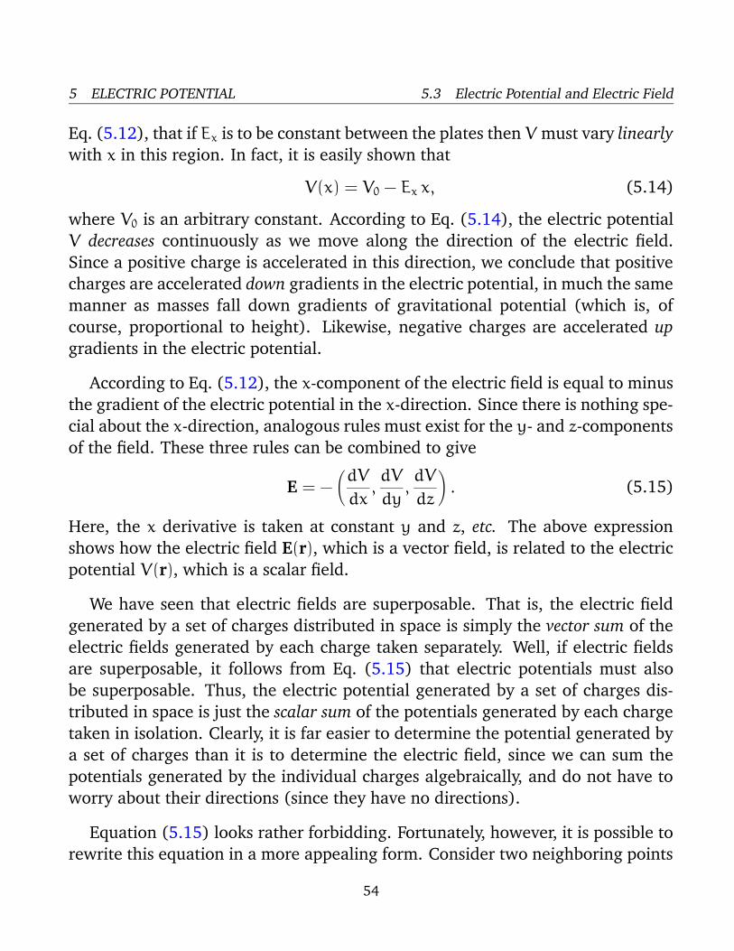
5 ELECTRIC POTENTIAL 5.3 Electric Potential and Electric Field
Eq. (5.12), that if Ex is to be constant between the plates then V must vary linearly
with x in this region. In fact, it is easily shown that
V(x) = V0 − Ex x, (5.14)
where V0 is an arbitrary constant. According to Eq. (5.14), the electric potential
V decreases continuously as we move along the direction of the electric field.
Since a positive charge is accelerated in this direction, we conclude that positive
charges are accelerated down gradients in the electric potential, in much the same
manner as masses fall down gradients of gravitational potential (which is, of
course, proportional to height). Likewise, negative charges are accelerated up
gradients in the electric potential.
According to Eq. (5.12), the x-component of the electric field is equal to minus
the gradient of the electric potential in the x-direction. Since there is nothing spe-
cial about the x-direction, analogous rules must exist for the y- and z-components
of the field. These three rules can be combined to give
E = −
(
dV
dx,dV
dy,dV
dz
)
. (5.15)
Here, the x derivative is taken at constant y and z, etc. The above expression
shows how the electric field E(r), which is a vector field, is related to the electric
potential V(r), which is a scalar field.
We have seen that electric fields are superposable. That is, the electric field
generated by a set of charges distributed in space is simply the vector sum of the
electric fields generated by each charge taken separately. Well, if electric fields
are superposable, it follows from Eq. (5.15) that electric potentials must also
be superposable. Thus, the electric potential generated by a set of charges dis-
tributed in space is just the scalar sum of the potentials generated by each charge
taken in isolation. Clearly, it is far easier to determine the potential generated by
a set of charges than it is to determine the electric field, since we can sum the
potentials generated by the individual charges algebraically, and do not have to
worry about their directions (since they have no directions).
Equation (5.15) looks rather forbidding. Fortunately, however, it is possible to
rewrite this equation in a more appealing form. Consider two neighboring points
54

5 ELECTRIC POTENTIAL 5.3 Electric Potential and Electric Field
A and B. Suppose that dr = (dx, dy, dz) is the vector displacement of point B
relative to point A. Let dV be the difference in electric potential between these
two points. Suppose that we travel from A to B by first moving a distance dx
along the x-axis, then moving dy along the y-axis, and finally moving dz along
the z-axis. The net increase in the electric potential dV as we move from A to B
is simply the sum of the increases dxV as we move along the x-axis, dyV as we
move along the y-axis, and dzV as we move along the z-axis:
dV = dxV + dyV + dzV. (5.16)
But, according to Eq. (5.15), dxV = −Ex dx, etc. So, we obtain
dV = −Ex dx − Ey dy − Ez dy, (5.17)
which is equivalent to
dV = −E·dr = −E dr cos θ, (5.18)
where θ is the angle subtended between the vector dr and the local electric field
E. Note that dV attains its most negative value when θ = 0. In other words,
the direction of the electric field at point A corresponds to the direction in which
the electric potential V decreases most rapidly. A positive charge placed at point
A is accelerated in this direction. Likewise, a negative charge placed at A is
accelerated in the direction in which the potential increases most rapidly (i.e.,
θ = 180). Suppose that we move from point A to a neighboring point B in a
direction perpendicular to that of the local electric field (i.e., θ = 90). In this
case, it follows from Eq. (5.18) that the points A and B lie at the same electric
potential (i.e., dV = 0). The locus of all the points in the vicinity of point A which
lie at the same potential as A is a plane perpendicular to the direction of the local
electric field. More generally, the surfaces of constant electric potential, the so-
called equipotential surfaces, exist as a set of non-interlocking surfaces which are
everywhere perpendicular to the direction of the electric field. Figure 5.1 shows
the equipotential surfaces (dashed lines) and electric field-lines (solid lines) gen-
erated by a positive point charge. In this case, the equipotential surfaces are
spheres centred on the charge.
In Sect. 4.3, we found that the electric field immediately above the surface
of a conductor is directed perpendicular to that surface. Thus, it is clear that
55

5 ELECTRIC POTENTIAL 5.4 Electric Potential of a Point Charge
Figure 5.1: The equipotential surfaces (dashed lines) and the electric field-lines (solid lines) of a
positive point charge.
the surface of a conductor must correspond to an equipotential surface. In fact,
since there is no electric field inside a conductor (and, hence, no gradient in the
electric potential), it follows that the whole conductor (i.e., both the surface and
the interior) lies at the same electric potential.
5.4 Electric Potential of a Point Charge
Let us calculate the electric potential V(r) generated by a point charge q located
at the origin. It is fairly obvious, by symmetry, and also by looking at Fig. 5.1,
that V is a function of r only, where r is the radial distance from the origin.
Thus, without loss of generality, we can restrict our investigation to the potential
V(x) generated along the positive x-axis. The x-component of the electric field
generated along this axis takes the form
Ex(x) =q
4πε0 x2. (5.19)
Both the y- and z-components of the field are zero. According to Eq. (5.12), Ex(x)
and V(x) are related via
Ex(x) = −dV(x)
dx. (5.20)
56

5 ELECTRIC POTENTIAL 5.5 Worked Examples
Thus, by integration,
V(x) =q
4πε0 x+ V0, (5.21)
where V0 is an arbitrary constant. Finally, making use of the fact that V = V(r),
we obtain
V(r) =q
4πε0 r. (5.22)
Here, we have adopted the common convention that the potential at infinity is
zero. A potential defined according to this convention is called an absolute poten-
tial.
Suppose that we have N point charges distributed in space. Let the ith charge
qi be located at position vector ri. Since electric potential is superposable, and
is also a scalar quantity, the absolute potential at position vector r is simply the
algebraic sum of the potentials generated by each charge taken in isolation:
V(r) =
N∑
i=1
qi
4πε0 |r − ri|. (5.23)
The work W we would perform in taking a charge q from infinity and slowly
moving it to point r is the same as the increase in electric potential energy of
the charge during its journey [see Eq. (5.4)]. This, by definition, is equal to the
product of the charge q and the increase in the electric potential. This, finally, is
the same as q times the absolute potential at point r: i.e.,
W = q V(r). (5.24)
5.5 Worked Examples
Example 5.1: Charge in a uniform electric field
Question: A charge of q = +1.20 µC is placed in a uniform x-directed electric
field of magnitude Ex = 1.40 × 10³ N C−1. How much work must be performed in
order to move the charge a distance c = −3.50 cm in the x-direction? What is the
potential difference between the initial and final positions of the charge? If the
57

5 ELECTRIC POTENTIAL 5.5 Worked Examples
electric field is produced by two oppositely charged parallel plates separated by
a distance d = 5.00 cm, what is the potential difference between the plates?
Solution: Let us denote the initial and final positions of the charge A and B,
respectively. The work which we must perform in order to move the charge from
A to B is minus the product of the electrostatic force on the charge due to the
electric field (since the force we exert on the charge is minus this force) and the
distance that the charge moves in the direction of this force [see Eq. (5.1)]. Thus,
W = −q Ex c = −(1.2 × 10⁻⁶) (1.40 × 10³) (−3.50 × 10⁻²) = +5.88 × 10⁻⁵ J.
Note that the work is positive. This makes sense, because we would have to do
real work (i.e., we would lose energy) in order to move a positive charge in the
opposite direction to an electric field (i.e., against the direction of the electrostatic
force acting on the charge).
The work done on the charge goes to increase its electric potential energy, so
PB − PA = W. By definition, this increase in potential energy is equal to the
product of the potential difference VB − VA between points B and A, and the
magnitude of the charge q. Thus,
q (VB − VA) = PB − PA = W = −q Ex c,
giving
VB − VA = −Ex c = −(1.40 × 10³) (−3.50 × 10⁻²) = 49.0 V.
Note that the electric field is directed from point B to point A, and that the former
point is at a higher potential than the latter.
It is clear, from the above formulae, that the magnitude of the potential differ-
ence between two points in a uniform electric field is simply the product of the
electric field-strength and the distance between the two points (in the direction
of the field). Thus, the potential difference between the two metal plates is
∆V = Ex d = (1.40 × 10³) (5.00 × 10⁻²) = 70.0 V.
If the electric field is directed from plate 1 (the positively charged plate) to plate
2 (the negatively charged plate) then the former plate is at the higher potential.
58

5 ELECTRIC POTENTIAL 5.5 Worked Examples
Example 5.2: Motion of an electron in an electric field
Question: An electron in a television set is accelerated from the cathode to the
screen through a potential difference of +1000 V. The screen is 35 mm from the
cathode. What is the net change in the potential energy of the electron during
the acceleration process? How much work is done by the electric field in accel-
erating the electron? What is the speed of the electron when it strikes the screen?
Solution: Let call the cathode point A and the screen point B. We are told that
the potential difference between points B and A is +1000 V, so
VB − VA = 1000 V.
By definition, the difference in electric potential energy of some charge q at points
B and A is the product of the charge and the difference in electric potential
between these points. Thus,
PB − PA = q (VB − VA) = (−1.6 × 10⁻¹⁹) (1000) = −1.6 × 10⁻¹⁶ J,
since q = −1.6 × 10⁻¹⁹ C for an electron. Note that the potential energy of the
electron decreases as it is accelerated towards the screen. As we have seen, the
electric potential energy of a charge is actually held in the surrounding electric
field. Thus, a decrease in the potential energy of the charge corresponds to a
reduction in the energy of the field. In this case, the energy of the field decreases
because it does work W ′ on the charge. Clearly, the work done (i.e., energy lost)
by the field equals the decrease in potential energy of the charge,
W ′ = −∆P.
Thus,
W ′ = 1.6 × 10⁻¹⁶ J.
The total energy E of the electron is made up of two components—the electric
potential energy P, and the kinetic energy K. Thus,
E = P + K.
59

5 ELECTRIC POTENTIAL 5.5 Worked Examples
Of course,
K =1
2m v2,
where m = 9.11 × 10⁻³¹ kg is the mass of the electron, and v its speed. By
conservation of energy, E is a constant of the motion, so
KB − KA = ∆K = −∆P.
In other words, the decrease in electric potential energy of the electron, as it is
accelerated towards the screen, is offset by a corresponding increase in its kinetic
energy. Assuming that the electron starts from rest (i.e. vA = 0), it follows that
1
2m v 2
B = −∆P,
or
vB =
√
√
√
√
−2 ∆P
m=
√
√
√
√
−2 (−1.6 × 10⁻¹⁶)
9.11 × 10−31= 1.87 × 10⁷ m s−1.
Note that the distance between the cathode and the screen is immaterial in this
problem. The final speed of the electron is entirely determined by its charge, its
initial velocity, and the potential difference through which it is accelerated.
Example 5.3: Electric potential due to point charges
Question: A particle of charge q1 = +6.0 µC is located on the x-axis at the point
x1 = 5.1 cm. A second particle of charge q2 = −5.0 µC is placed on the x-axis at
x2 = −3.4 cm. What is the absolute electric potential at the origin (x = 0)? How
much work must we perform in order to slowly move a charge of q3 = −7.0 µC
from infinity to the origin, whilst keeping the other two charges fixed?
Solution: The absolute electric potential at the origin due to the first charge is
V1 = ke
q1
x1
= (8.988 × 10⁹)(6 × 10⁻⁶)
(5.1 × 10⁻²)= 1.06 × 10⁶ V.
Likewise, the absolute electric potential at the origin due to the second charge is
V2 = ke
q2
|x2|= (8.988 × 10⁹)
(−5 × 10⁻⁶)
(3.4 × 10⁻²)= −1.32 × 10⁶ V.
60

5 ELECTRIC POTENTIAL 5.5 Worked Examples
The net potential V at the origin is simply the algebraic sum of the potentials due
to each charge taken in isolation. Thus,
V = V1 + V2 = −2.64 × 10⁵ V.
The work W which we must perform in order to slowly moving a charge q3
from infinity to the origin is simply the product of the charge and the potential
difference V between the end and beginning points. Thus,
W = q3 V = (−7 × 10⁻⁶) (−2.64 × 10⁵) = 1.85 J.
Example 5.4: Electric potential due to point charges
ac
b cq
b
aq
qx
y
Question: Suppose that three point charges, qa, qb, and qc, are arranged at the
vertices of a right-angled triangle, as shown in the diagram. What is the absolute
electric potential of the third charge if qa = −6.0 µC, qb = +4.0 µC, qc = +2.0 µC,
a = 4.0 m, and b = 3.0 m? Suppose that the third charge, which is initially at
rest, is repelled to infinity by the combined electric field of the other two charges,
which are held fixed. What is the final kinetic energy of the third charge?
Solution: The absolute electric potential of the third charge due to the presence
of the first charge is
Va = ke
qa
c= (8.988 × 10⁹)
(−6 × 10⁻⁶)
(√
42 + 32)= −1.08 × 10⁴ V,
61

5 ELECTRIC POTENTIAL 5.5 Worked Examples
where use has been made of the Pythagorean theorem. Likewise, the absolute
electric potential of the third charge due to the presence of the second charge is
Vb = ke
qb
b= (8.988 × 10⁹)
(4 × 10⁻⁶)
(3)= 1.20 × 10⁴ V.
The net absolute potential of the third charge Vc is simply the algebraic sum of
the potentials due to the other two charges taken in isolation. Thus,
Vc = Va + Vb = 1.20 × 10³ V.
The change in electric potential energy of the third charge as it moves from its
initial position to infinity is the product of the third charge, qc, and the difference
in electric potential (−Vc) between infinity and the initial position. It follows that
∆P = −qc Vc = −(2 × 10⁻⁶) (1.2 × 10³) = −2.40 × 10⁻³ J.
This decrease in the potential energy of the charge is offset by a corresponding
increase ∆K = −∆P in its kinetic energy. Since the initial kinetic energy of the
third charge is zero (because it is initially at rest), the final kinetic energy is
simply
K = ∆K = −∆P = 2.40 × 10⁻³ J.
62

6 CAPACITANCE
6 Capacitance
6.1 Charge Storage
Consider a hollow metal sphere mounted on an insulating stand. The sphere
is initially grounded so that no excess charge remains on it. Suppose that we
introduce a metal ball, suspended on an insulating thread, through a small hole
in the sphere, and then fill in the hole with a metal plug. Let the ball carry a
charge +Q. What distribution of charge is induced on the hollow sphere as a
result of introducing the positive charge into the cavity?
To answer this question we make use of Gauss’ law (see Sect. 4.2)
ΦE =
∮
E · dS =Q
ε0
. (6.1)
Assuming that the metal ball is placed at the centre of the hollow sphere, we
can use symmetry arguments to deduce that the electric field depends only on
the radial distance r from the centre, and is everywhere directed radially away
from the ball. Let us choose a spherical gaussian surface, centred on the ball,
which runs through the interior of the hollow metal sphere. We know that the
electric field inside a conductor is everywhere zero (see Sect. 4.6), so the electric
flux ΦE through the surface is also zero. It follows from Gauss’ law that zero
net charge is enclosed by the surface. Now, there is a charge +Q on the ball at
the centre of the hollow sphere, so there must be an equal and opposite charge
−Q distributed over the interior surface of the sphere (recall that any charge
carried on a conductor must reside on its surface). Furthermore, since the sphere
is insulated, and was initially uncharged, a charge +Q must be distributed over
its exterior surface. Thus, when the charge +Q is introduced into the centre of
the sphere, there is a redistribution of charge in the sphere such that a positive
charge +Q is repelled to its exterior surface, leaving a negative charge −Q on the
interior surface. (In actuality, free electrons are attracted to the interior surface,
exposing positive charges on the exterior surface). Further use of Gauss’ law
shows that the electric field between the charged ball and the interior surface of
the sphere is the same as that generated by a point charge +Q located at the
63

6 CAPACITANCE 6.2 Breakdown
centre of the sphere. Likewise, for the electric field exterior to the sphere. The
electric field inside the conducting sphere is, of course, zero.
Suppose, finally, that the ball is moved so that it touches the inside of the
hollow sphere. The charge −Q on the interior surface of the sphere cancels the
charge +Q on the ball, leaving the charge +Q distributed over its exterior sur-
face. Thus, the effect of touching the ball to the inside of the sphere is to transfer
the charge +Q from the ball to the exterior surface of the sphere. In principle, we
can repeat this process, again and again, until a very large amount of charge is ac-
cumulated on the outside of the sphere. The idea of transferring charge from one
conductor to another by means of internal contact is the theoretical basis of the
Van de Graaff generator. In this type of device, charge is continuously transmitted
to a conducting sphere by means of a moving belt charged by friction.
6.2 Breakdown
Is there any practical limit to the charge Q which can be accumulated on the
conducting sphere of a Van de Graaff generator? Well, we know that the field
outside the sphere is just the same as if the charge Q were placed at the centre of
the sphere. In fact, the electric field is at its most intense just above the surface
of the sphere, where it has the magnitude E = Q/(4πε0 a2). Here, a is the radius
of the sphere. Air (assuming that the sphere is surrounded by air) is generally a
very good insulator. However, air ceases to be an insulator when the electric field-
strength through it exceeds some critical value which is about Ecrit ∼ 106 V m−1.
This phenomenon is known as breakdown, and is associated with the formation of
sparks. The explanation of breakdown is quite straightforward. Air naturally con-
tains a very small fraction of ionized molecules (not enough to prevent air from
being an insulator). In an electric field, these ionized molecules are constantly be-
ing accelerated, and then crashing into neutral molecules. As the strength of the
field is increased, the ionized molecules are accelerated to ever higher energies
before crashing into the neutral molecules. Eventually, a critical field-strength
Ecrit is reached at which the ionized molecules are accelerated to a sufficiently
high energy that they ionize the neutral molecules when they hit them. At this
64

6 CAPACITANCE 6.2 Breakdown
point, a chain reaction takes place which rapidly leads to the almost complete
ionization of the air. Thus, the air makes an almost instantaneous transition from
a good insulator to a good conductor. It follows that the charge Q on the con-
ducting sphere of a Van de Graaff generator can never exceed the critical value
Qcrit = 4πε0 a2 Ecrit, because for Q ≥ Qcrit the electric field around the sphere is
sufficiently intense to cause breakdown. Of course, when breakdown occurs the
charge on the sphere is conducted to earth.
The phenomenon of breakdown sets an upper limit on the charge which can
be stored on a conductor. There is, however, another important factor which
affects the onset of breakdown. This is best illustrated in the following simple
example. Suppose that we have two charged conducting spheres of radii a and
b, respectively, which are connected by a long conducting wire. The wire allows
charge to move back and forth between the spheres until they reach the same
potential (recall that the electric potential is uniform in a conductor). Let Qa be
the charge on the first sphere, and Qb the charge on the second sphere. Of course,
the total charge Q = Qa + Qb carried by the two spheres is a conserved quantity.
The electric field generated by each sphere is the same as if the charge on that
sphere were concentrated at its centre. Assuming that the wire is sufficiently long
that the two spheres do not affect one another very much, the absolute potential
of the first sphere is Va = Qa/(4πε0 a), whereas that of the second sphere is
Vb = Qb/(4πε0 b) [see Eq. (5.22)]. Since Va = Vb, we find that
Qa
Q=
a
a + b, (6.2)
Qb
Q=
b
a + b. (6.3)
Note that if the second sphere is much smaller than the first (i.e., if b a) then
the larger sphere grabs the lion’s share of the charge:
Qa
Qb
=a
b 1. (6.4)
The electric field-strengths just above the surfaces of the two spheres are Ea =
Qa/(4πε0 a2) and Eb = Qb/(4πε0 b2), respectively. Thus, the ratio of the field-
65

6 CAPACITANCE 6.2 Breakdown
strengths generated in the immediate vicinities of the two spheres is
Eb
Ea
=Qb
Qa
a2
b2=
a
b. (6.5)
Clearly, if b a then the field just above the smaller sphere is far stronger than
that above the larger one. Suppose that the total charge Q0 on the two spheres
is gradually increased until breakdown occurs. Since Eb Ea, it follows that
breakdown always occurs above the smaller sphere.
Equation (6.5) is a special case of a far more general rule: i.e., the electric
field-strength above some point on the surface of a conductor is inversely pro-
portional to the local radius of curvature of the surface. It is clear that if we
wish to store significant amounts of charge on a conductor then the surface of
the conductor must be made as smooth as possible. Any sharp spikes on the sur-
face possess relatively small radii of curvature. Intense local electric fields are
generated above these spikes whenever the conductor is charged. These fields
can easily exceed the critical field for the breakdown of air, leading to sparking,
and the eventual loss of the charge on the conductor. Sparking tends to be very
destructive because of its highly localized nature, which leads inevitably to very
large electric currents, and, hence, to intense heating.
Clouds can acquire very large negative charges during thunderstorms. An
equal and opposite positive charge is induced on the surface of the Earth. The
electric field generated between the clouds and the Earth can become sufficiently
large to cause breakdown in the atmosphere, giving rise to the phenomenon
which we call lightning. Let us consider the various factors which determine
where lightning strikes. Breakdown starts at cloud level, as a so-called “dark
leader” of ionized air traces out a path towards the ground. When it comes within
about 10 meters of ground level, a second dark leader comes up from the ground
to meet it. Once the two leaders meet, and a conducting path is established, the
lightning strike proper occurs. Note that, contrary to popular opinion, the light-
ning strike travels upwards from the Earth to the clouds. It is clear that lightning
“strikes” a particular object on the ground because the object emits a dark leader:
i.e., because breakdown takes place just above the object. In a thunderstorm, the
ground, and the objects upon it, acts essentially like a charged conductor with a
66

6 CAPACITANCE 6.3 Capacitance
convoluted surface. Thus, any “spikes” on the ground (e.g., a person standing in
a field, a radio mast, a lightning rod) are comparatively more likely to be hit by
lightning, because the electric field-strength above these points is relatively large,
which facilitates breakdown.
6.3 Capacitance
As we have seen, the amount of charge which can be stored on a conductor is
limited by the electric field-strength just above its surface, which is not allowed
to exceed a certain critical value, Ecrit. Unfortunately, the field-strength varies
from point to point across the surface (unless the surface possesses a constant
radius of curvature). It is, therefore, generally convenient to parameterize the
maximum field-strength above the surface of a conductor in terms of the voltage
difference V between the conductor and either infinity or another conductor. The
point is that V , unlike the electric field-strength, is a constant over the surface,
and can, therefore, be specified unambiguously.
How do we tell the difference between a good and a bad charge storage de-
vice? Well, a good charge storage device must be capable of storing a large
amount of charge without causing breakdown. Likewise, a bad charge storage
device is only capable of storing a small amount of charge before breakdown oc-
curs. Thus, if we place a charge Q in a good storage device then the electric fields
generated just above the surface of the device should be comparatively weak. In
other words, the voltage V should be relatively small. A convenient measure of
the ability of a device to store electric charge is its capacitance, C, which is defined
as the ratio of Q over V:
C =Q
V. (6.6)
Obviously, a good charge storage device possesses a high capacitance. Note that
the capacitance of a given charge storage device is a constant which depends on
the dimensions of the device, but is independent of either Q or V . This follows
from the linear nature of the laws of electrostatics: i.e., if we double the charge
on the device, then we double the electric fields generated around the device,
and so we double the voltage difference between the device and (say) infinity.
67

6 CAPACITANCE 6.4 Dielectrics
In other words, V ∝ Q. The units of capacitance are called farads (F), and are
equivalent to coulombs per volt:
1 F ≡ 1 C V−1. (6.7)
A farad is actually a pretty unwieldy unit. In fact, most of the capacitors found in
electronic circuits have capacitances in the micro-farad range.
Probably the simplest type of capacitor is the so-called parallel plate capacitor,
which consists of two parallel conducting plates, one carrying a charge +Q and
the other a charge −Q, separated by a distance d. Let A be the area of the two
plates. It follows that the charge densities on the plates are σ and −σ, respec-
tively, where σ = Q/A. Now, we have already seen (in Sect. 4.5) that the electric
field generated between two oppositely charged parallel plates is uniform, and of
magnitude E = σ/ε0. The field is directed perpendicular to the plates, and runs
from the positively to the negatively charged plate. Note that this result is only
valid if the spacing between the plates is much less than their typical dimensions.
According to Eq. (4.8), the potential difference V between the plates is given by
V = E d =σ d
ε0
=Q d
ε0 A, (6.8)
where the positively charged plate is at the higher potential. It follows from
Eq. (6.6) that the capacitance of a parallel plate capacitor takes the form
C =ε0 A
d. (6.9)
Note that the capacitance is proportional to the area of the plates, and inversely
proportional to their perpendicular spacing. It follows that a good parallel plate
capacitor possesses closely spaced plates of large surface area.
6.4 Dielectrics
Strictly speaking, the expression (6.9) for the capacitance of a parallel plate ca-
pacitor is only valid if the region between plates is a vacuum. However, this
expression turns out to be a pretty good approximation if the region is filled with
68

6 CAPACITANCE 6.4 Dielectrics
Material K
Vacuum 1
Air 1.00059
Water 80
Paper 3.5
Pyrex 4.5
Teflon 2.1
Table 6.1: Dielectric constants of various common materials.
air. But, what happens if the region between the plates is filled by an insulating
material such as glass or plastic?
We could investigate this question experimentally. Suppose that we started
with a charged parallel plate capacitor, whose plates were separated by a vacuum
gap, and which was disconnected from any battery or other source of charge. We
could measure the voltage difference V0 between the plates using a voltmeter.
Suppose that we inserted a slab of some insulating material (e.g., glass) into the
gap between the plates, and then re-measured the voltage difference between
the plates. We would find that the new voltage difference V was less than V0,
despite that fact that the charge Q on the plates was unchanged. Let us denote
the voltage ratio V0/V as K. Since, C = Q/V , it follows that the capacitance
of the capacitor must have increased by a factor K when the insulating slab was
inserted between the plates.
An insulating material which has the effect of increasing the capacitance of a
vacuum-filled parallel plate capacitor, when it is inserted between its plates, is
called a dielectric material, and the factor K by which the capacitance is increased
is called the dielectric constant of that material. Of course, K varies from material
to material. A few sample values are given in Table 6.1. Note, however, that K is
always greater than unity, so filling the gap between the plates of a parallel plate
capacitor with a dielectric material always increases the capacitance of the device
to some extent. On the other hand, K for air is only 0.06 percent greater than K
for a vacuum (i.e., K = 1), so an air-filled capacitor is virtually indistinguishable
from a vacuum-filled capacitor.
69

6 CAPACITANCE 6.4 Dielectrics
The formula for the capacitance of a dielectric-filled parallel plate capacitor is
C =ε A
d, (6.10)
where
ε = K ε0 (6.11)
is called the permittivity of the dielectric material between the plates. Note that
the permittivity ε of a dielectric material is always greater than the permittivity
of a vacuum ε0
How do we explain the reduction in voltage which occurs when we insert a
dielectric between the plates of a vacuum-filled parallel plate capacitor? Well,
if the voltage difference between the plates is reduced then the electric field be-
tween the plates must be reduced by the same factor. In other words, the electric
field E0 generated by the charge stored on the capacitor plates must be partially
canceled out by an opposing electric field E1 generated by the dielectric itself
when it is placed in an external electric field. What is the cause of this opposing
field? It turns out that the opposing field is produced by the polarization of the
constituent molecules of the dielectric when they are placed in an electric field
(see Sect. 3.4). If E0 is sufficiently small then the degree of polarization of each
molecule is proportional to the strength of the polarizing field E0. It follows that
the strength of the opposing field E1 is also proportional to E0. In fact, the con-
stant of proportionality is 1 − 1/K, so E1 = (1 − 1/K) E0. The net electric field
between the plates is E0 − E1 = E0/K. Hence, both the field and voltage between
the plates are reduced by a factor K with respect to the vacuum case. In principle,
the dielectric constant K of a dielectric material can be calculated from the prop-
erties of the molecules which make up the material. In practice, this calculation
is too difficult to perform, except for very simple molecules. Note that the result
that the degree of polarization of a polarizable molecule is proportional to the
external electric field-strength E0 breaks down if E0 becomes too large (just as
Hooke’s law breaks down if we pull too hard on a spring). Fortunately, however,
the field-strengths encountered in conventional laboratory experiments are not
generally large enough to invalidate this result.
We have seen that when a dielectric material of dielectric constant K is placed
70

6 CAPACITANCE 6.5 Capacitors in Series and in Parallel
in the uniform electric field generated between the plates of a parallel plate ca-
pacitor then the material polarizes, giving rise to a reduction of the field-strength
between the plates by some factor K. Since there is nothing particularly spe-
cial about the electric field between the plates of a capacitor, we surmise that
this result is quite general. Thus, if space is filled with a dielectric medium then
Coulomb’s law is rewritten as
f =q q ′
4πε r2, (6.12)
and the formula for the electric field generated by a point charge becomes
E =q
4πε r2, (6.13)
etc. Clearly, in a dielectric medium, the laws of electrostatics take exactly the
same form as in a vacuum, except that the permittivity of free space ε0 is replaced
by the permittivity ε = K ε0 of the medium. Dielectric materials have the general
effect of reducing the electric fields and potential differences generated by electric
charges. Such materials are extremely useful because they inhibit breakdown.
For instance, if we fill a parallel plate capacitor with a dielectric material then
we effectively increase the amount of charge we can store on the device before
breakdown occurs.
6.5 Capacitors in Series and in Parallel
Capacitors are one of the standard components in electronic circuits. Moreover,
complicated combinations of capacitors often occur in practical circuits. It is,
therefore, useful to have a set of rules for finding the equivalent capacitance of
some general arrangement of capacitors. It turns out that we can always find the
equivalent capacitance by repeated application of two simple rules. These rules
related to capacitors connected in series and in parallel.
Consider two capacitors connected in parallel: i.e., with the positively charged
plates connected to a common “input” wire, and the negatively charged plates
attached to a common “output” wire—see Fig. 6.1. What is the equivalent capac-
itance between the input and output wires? In this case, the potential difference
71

6 CAPACITANCE 6.5 Capacitors in Series and in Parallel
+
1C
C2
+
Figure 6.1: Two capacitors connected in parallel.
V across the two capacitors is the same, and is equal to the potential difference
between the input and output wires. The total charge Q, however, stored in the
two capacitors is divided between the capacitors, since it must distribute itself
such that the voltage across the two is the same. Since the capacitors may have
different capacitances, C1 and C2, the charges Q1 and Q2 may also be different.
The equivalent capacitance Ceq of the pair of capacitors is simply the ratio Q/V ,
where Q = Q1 + Q2 is the total stored charge. It follows that
Ceq =Q
V=
Q1 + Q2
V=
Q1
V+
Q2
V, (6.14)
giving
Ceq = C1 + C2. (6.15)
Here, we have made use of the fact that the voltage V is common to all three
capacitors. Thus, the rule is:
The equivalent capacitance of two capacitors connected in parallel is the sum
of the individual capacitances.
For N capacitors connected in parallel, Eq. (6.15) generalizes to Ceq =∑N
i=1 Ci.
Consider two capacitors connected in series: i.e., in a line such that the positive
plate of one is attached to the negative plate of the other—see Fig. 6.2. In fact,
72

6 CAPACITANCE 6.5 Capacitors in Series and in Parallel
2C
+ +
C1
Figure 6.2: Two capacitors connected in series.
let us suppose that the positive plate of capacitor 1 is connected to the “input”
wire, the negative plate of capacitor 1 is connected to the positive plate of capac-
itor 2, and the negative plate of capacitor 2 is connected to the “output” wire.
What is the equivalent capacitance between the input and output wires? In this
case, it is important to realize that the charge Q stored in the two capacitors is
the same. This is most easily seen by considering the “internal” plates: i.e., the
negative plate of capacitor 1, and the positive plate of capacitor 2. These plates
are physically disconnected from the rest of the circuit, so the total charge on
them must remain constant. Assuming, as seems reasonable, that these plates
carry zero charge when zero potential difference is applied across the two capac-
itors, it follows that in the presence of a non-zero potential difference the charge
+Q on the positive plate of capacitor 2 must be balanced by an equal and op-
posite charge −Q on the negative plate of capacitor 1. Since the negative plate
of capacitor 1 carries a charge −Q, the positive plate must carry a charge +Q.
Likewise, since the positive plate of capacitor 2 carries a charge +Q, the negative
plate must carry a charge −Q. The net result is that both capacitors possess the
same stored charge Q. The potential drops, V1 and V2, across the two capacitors
are, in general, different. However, the sum of these drops equals the total po-
tential drop V applied across the input and output wires: i.e., V = V1 + V2. The
equivalent capacitance of the pair of capacitors is again Ceq = Q/V . Thus,
1
Ceq=
V
Q=
V1 + V2
Q=
V1
Q+
V2
Q, (6.16)
giving1
Ceq=
1
C1
+1
C2
. (6.17)
Here, we have made use of the fact that the charge Q is common to all three
capacitors. Hence, the rule is:
73

6 CAPACITANCE 6.6 Energy Stored by Capacitors
The reciprocal of the equivalent capacitance of two capacitors connected in
series is the sum of the reciprocals of the individual capacitances.
For N capacitors connected in series, Eq. (6.17) generalizes to 1/Ceq =∑N
i=1(1/Ci).
6.6 Energy Stored by Capacitors
Let us consider charging an initially uncharged parallel plate capacitor by trans-
ferring a charge Q from one plate to the other, leaving the former plate with
charge −Q and the later with charge +Q. Of course, once we have transferred
some charge, an electric field is set up between the plates which opposes any
further charge transfer. In order to fully charge the capacitor, we must do work
against this field, and this work becomes energy stored in the capacitor. Let us
calculate this energy.
Suppose that the capacitor plates carry a charge q and that the potential dif-
ference between the plates is V . The work we do in transferring an infinitesimal
amount of charge dq from the negative to the positive plate is simply
dW = V dq. (6.18)
In order to evaluate the total work W(Q) done in transferring the total charge Q
from one plate to the other, we can divide this charge into many small increments
dq, find the incremental work dW done in transferring this incremental charge,
using the above formula, and then sum all of these works. The only complication
is that the potential difference V between the plates is a function of the total
transferred charge. In fact, V(q) = q/C, so
dW =q dq
C. (6.19)
Integration yields
W(Q) =
∫Q
0
q dq
C=
Q2
2 C. (6.20)
Note, again, that the work W done in charging the capacitor is the same as the
energy stored in the capacitor. Since C = Q/V , we can write this stored energy
74

6 CAPACITANCE 6.6 Energy Stored by Capacitors
in one of three equivalent forms:
W =Q2
2 C=
C V2
2=
Q V
2. (6.21)
These formulae are valid for any type of capacitor, since the arguments that we
used to derive them do not depend on any special property of parallel plate ca-
pacitors.
Where is the energy in a parallel plate capacitor actually stored? Well, if we
think about it, the only place it could be stored is in the electric field generated
between the plates. This insight allows us to calculate the energy (or, rather, the
energy density) of an electric field.
Consider a vacuum-filled parallel plate capacitor whose plates are of cross
sectional area A, and are spaced a distance d apart. The electric field E between
the plates is approximately uniform, and of magnitude σ/ε0, where σ = Q/A, and
Q is the charge stored on the plates. The electric field elsewhere is approximately
zero. The potential difference between the plates is V = E d. Thus, the energy
stored in the capacitor can be written
W =C V2
2=
ε0 A E2 d2
2 d=
ε0 E2 Ad
2, (6.22)
where use has been made of Eq. (6.9). Now, A d is the volume of the field-filled
region between the plates, so if the energy is stored in the electric field then the
energy per unit volume, or energy density, of the field must be
w =ε0 E2
2. (6.23)
It turns out that this result is quite general. Thus, we can calculate the energy
content of any electric field by dividing space into little cubes, applying the above
formula to find the energy content of each cube, and then summing the energies
thus obtained to obtain the total energy.
It is easily demonstrated that the energy density in a dielectric medium is
w =ε E2
2, (6.24)
75

6 CAPACITANCE 6.7 Worked Examples
where ε = K ε0 is the permittivity of the medium. This energy density consists of
two elements: the energy density ε0 E2/2 held in the electric field, and the energy
density (K − 1) ε0 E2/2 held in the dielectric medium (this represents the work
done on the constituent molecules of the dielectric in order to polarize them).
6.7 Worked Examples
Example 6.1: Parallel plate capacitor
Question: A parallel plate capacitor consists of two metal plates, each of area
A = 150 cm2, separated by a vacuum gap d = 0.60 cm thick. What is the ca-
pacitance of this device? What potential difference must be applied between the
plates if the capacitor is to hold a charge of magnitude Q = 1.00 × 10⁻³ µC on
each plate?
Solution: Making use of formula (6.9), the capacitance C is given by
C =(8.85 × 10⁻¹²) (150 × 10−4)
(0.6 × 10⁻²)= 2.21 × 10−11 = 22.1 pF.
The voltage difference V between the plates and the magnitude of the charge
Q stored on each plate are related via C = Q/V , or V = Q/C. Hence, if Q =
1.00 × 10⁻³ µC then
V =(1.00 × 10⁻⁹)
(2.21 × 10⁻¹¹)= 45.2 V.
Example 6.2: Dielectric filled capacitor
Question: A parallel plate capacitor has a plate area of 50 cm2 and a plate sepa-
ration of 1.0 cm. A potential difference of V0 = 200 V is applied across the plates
with no dielectric present. The battery is then disconnected, and a piece of Bake-
lite (K = 4.8) is inserted which fills the region between the plates. What is the
capacitance, the charge on the plates, and the potential difference between the
76

6 CAPACITANCE 6.7 Worked Examples
plates, before and after the dielectric is inserted?
Answer: Before the dielectric is inserted, the space between the plates is presum-
ably filled with air. Since the dielectric constant of air is virtually indistinguish-
able from that of a vacuum, let us use the vacuum formula (6.9) to calculate the
initial capacitance C0. Thus,
C0 =ε0 A
d=
(8.85 × 10⁻¹²) (50 × 10−4)
(1 × 10⁻²)= 4.4 pF.
After the dielectric is inserted, the capacitance increases by a factor K, which in
this case is 4.8, so the new capacitance C is given by
C = K C0 = (4.8) (4.4 × 10⁻¹²) = 21 pF.
Before the dielectric is inserted, the charge Q0 on the plates is simply
Q0 = C0V0 = (4.4 × 10⁻¹²) (200) = 8.8 × 10⁻¹⁰ C.
After the dielectric is inserted, the charge Q is exactly the same, since the capac-
itor is disconnected, and so the charge cannot leave the plates. Hence,
Q = Q0 = 8.8 × 10⁻¹⁰ C.
The potential difference before the dielectric is inserted is given as V0 = 200 V.
The potential difference V after the dielectric is inserted is simply
V =Q
C=
(8.8 × 10⁻¹⁰)
(21 × 10−12)= 42 V.
Note, of course, that V = V0/K.
Example 6.3: Equivalent capacitance
Question: A 1 µF and a 2 µF capacitor are connected in parallel, and this pair of
capacitors is then connected in series with a 4 µF capacitor, as shown in the di-
agram. What is the equivalent capacitance of the whole combination? What is
77

6 CAPACITANCE 6.7 Worked Examples
4
Fµ
Fµ
Fµ
1
2
the charge on the 4 µF capacitor if the whole combination is connected across the
terminals of a 6 V battery? Likewise, what are the charges on the 1 µF and 2 µF
capacitors?
Answer: The equivalent capacitance of the 1 µF and 2 µF capacitors connected
in parallel is 1 + 2 = 3 µF. When a 3 µF capacitor is combined in series with a
4 µF capacitor, the equivalent capacitance of the whole combination is given by
1
Ceq=
1
(3 × 10⁻⁶)+
1
(4 × 10⁻⁶)=
(7)
(12 × 10−6)F−1,
and so
Ceq =(12 × 10−6)
(7)= 1.71 µF.
The charge delivered by the 6 V battery is
Q = CeqV = (1.71 × 10⁻⁶) (6) = 10.3 µC.
This is the charge on the 4 µF capacitor, since one of the terminals of the battery
is connected directly to one of the plates of this capacitor.
The voltage drop across the 4 µF capacitor is
V4 =Q
C4
=(10.3 × 10⁻⁶)
(4 × 10⁻⁶)= 2.57 V.
Thus, the voltage drop across the 1 µF and 2 µF combination must be V12 = 6 −
2.57 = 3.43 V. The charge stored on the 1 µF is given by
Q1 = C1 V12 = (1 × 10⁻⁶) (3.43) = 3.42 µC.
78

6 CAPACITANCE 6.7 Worked Examples
Likewise, the charge stored on the 2 µF capacitor is
Q2 = C2 V12 = (2 × 10⁻⁶) (3.43) = 6.84 µC.
Note that the total charge stored on the 1 µF and 2 µF combination is Q12 =
Q1 + Q2 = 10.3 µC, which is the same as the charge stored on the 4 µF capacitor.
This makes sense because the 1 µF and 2 µF combination and the 4 µF capacitor
are connected in series.
Example 6.4: Energy stored in a capacitor
Question: An air-filled parallel plate capacitor has a capacitance of 5.0 pF. A poten-
tial of 100 V is applied across the plates, which are 1.0 cm apart, using a storage
battery. What is the energy stored in the capacitor? Suppose that the battery is
disconnected, and the plates are moved until they are 2.0 cm apart. What now
is the energy stored in the capacitor? Suppose, instead, that the battery is left
connected, and the plates are again moved until they are 2.0 cm apart. What is
the energy stored in the capacitor in this case?
Answer: The initial energy stored in the capacitor is
W =C V2
2=
(5 × 10⁻¹²) (100)2
2= 2.5 × 10⁻⁸ J.
When the spacing between the plates is doubled, the capacitance of the capac-
itor is halved to 2.5 pF. If the battery is disconnected then this process takes place
at constant charge Q. Thus, it follows from the formula
W =Q2
2 C
that the energy stored in the capacitor doubles. So, the new energy is 5.0 ×10⁻⁸ J. Incidentally, the increased energy of the capacitor is accounted for by the
work done in pulling the capacitor plates apart (since these plates are oppositely
charged, they attract one another).
79

6 CAPACITANCE 6.7 Worked Examples
If the battery is left connected, then the capacitance is still halved, but now
the process takes place at constant voltage V . It follows from the formula
W =C V2
2
that the energy stored in the capacitor is halved. So, the new energy is 1.25 ×10⁻⁸ J. Incidentally, the energy lost by the capacitor is given to the battery (in
effect, it goes to re-charging the battery). Likewise, the work done in pulling the
plates apart is also given to the battery.
80

7 ELECTRIC CURRENT
7 Electric Current
7.1 Electric Circuits
A battery is a device possessing a positive and a negative terminal. Some process,
usually a chemical reaction, takes place inside the battery which causes positive
charge to migrate towards the positive terminal, and vice versa. This process
continues until the electric field set up between the two terminals is sufficiently
strong to inhibit any further charge migration.
An electric circuit is a conducting path, external to the battery, which allows
charge to flow from one terminal to the other. A simple circuit might consist of
a single strand of metal wire linking the positive and negative terminals. A more
realistic circuit possesses multiple branch points, so that charge can take many
different paths between the two terminals.
Suppose that a (positive) charge q is driven around the external circuit, from
the positive to the negative terminal, by the electric field set up between the
terminals. The work done on the charge by this field during its journey is q V ,
where V is the difference in electric potential between the positive and negative
terminals. We usually refer to V as the voltage of the battery: e.g., when we
talk of a 6 volt battery, what we actually mean is that the potential difference
between its two terminals is 6 V. Note, from Sect. 5, that the electrical work q V
done on the charge is completely independent of the route it takes between the
terminals. In other words, although there are, in general, many different paths
through the external circuit which the charge could take in order to get from the
positive to the negative terminal of the battery, the electrical energy which the
charge acquires in making this journey is always the same. Since, when analyzing
electrical circuits, we are primarily interested in energy (i.e., in the transformation
of the chemical energy of the battery into heat energy in some electric heating
element, or mechanical energy in some electric motor, etc.), it follows that the
property of a battery which primarily concerns us is its voltage. Hence, we do
not have to map out the electric field generated by a battery in order to calculate
how much energy this field gives to a charge q which goes around some external
81

7 ELECTRIC CURRENT 7.1 Electric Circuits
circuit connected to it. All we need to know is the potential difference V between
the two terminals of the battery. This is obviously an enormous simplification.
This section is only concerned with steady-state electric circuits powered by
batteries of constant voltage. Thus, the rate at which electric charge flows out of
the positive terminal of the battery into the external circuit must match the rate
at which charge flows from the circuit into the negative terminal of the battery,
otherwise charge would build up in either the battery or the circuit, which would
not correspond to a steady-state situation. The rate at which charge flows out
of the positive terminal is termed the electric current flowing out of the battery.
Likewise, the rate at which charge flows into the negative terminal is termed the
current flowing into the battery. Of course, these two currents must be the same
in a steady-state. Electric current is measured in units of amperes (A), which are
equivalent to coulombs per second:
1 A ≡ 1 C s−1. (7.1)
We can define the electric current I flowing at any particular point in the ex-
ternal circuit as follows. If an amount of charge dQ flows past this point in an
infinitesimal time interval dt then
I =dQ
dt. (7.2)
By convention, the direction of the current is taken to be the direction positive
charges would have to move in order to account for the flow of charge. In a
steady-state, the current at all points in the external circuit must remain constant
in time. We call this type of circuit a direct current (DC) circuit because the current
always flows in the same direction. There is a second type of circuit, called
an alternating current (AC) circuit, in which the current periodically switches
direction.
Consider a simple circuit in which a steady current I flows around a single
conducting wire connecting the positive and negative terminals of a battery of
voltage V . Let us suppose that the current is carried by positive charges flowing
around the external circuit from the positive to the negative terminal. In real-
ity, the current is carried by negative charges (i.e., by electrons) flowing in the
82

7 ELECTRIC CURRENT 7.2 Ohm’s Law
opposite direction, but for most purposes we can safely ignore this rather incon-
venient fact. Every charge q which flows around the external circuit experiences
a potential drop V . In order to flow around the circuit again, the charge must be
raised to the potential of the positive terminal of the battery. This process occurs
inside the battery, as the charge migrates from the negative to the positive ter-
minal. The energy q V required to move the charge between the two terminals
is derived from the energy released by the chemical reactions taking place inside
the battery.
The simple circuit described above is somewhat analogous to a small ski resort.
The charges flowing around the external circuit are like people skiing down the
ski-slope. The charges flow down a gradient of electric potential just as the people
ski down a gradient of gravitational potential. Note that the good skiers who
ski directly down the slope acquire exactly the same gravitational energy as the
poor skiers who ski from side to side. In both cases, the total acquired energy
depends only on the difference in height between the top and bottom of the slope.
Likewise, charges flowing around an external circuit acquire the same electrical
energy no matter what route they take, because the acquired energy only depends
on the potential difference between the two terminals of the battery. Once the
people in our ski resort reach the bottom of the slope, they must be lifted to
the top in a ski-lift before they can ski down it again. Thus, the ski-lift in our
resort plays an analogous role to the battery in our circuit. Of course, the ski-
lift must expend non-gravitational energy in order to lift skiers to the top of the
slope, in just the same manner as the battery must expend non-electrical energy
to move charges up a potential gradient. If the ski-lift runs out of energy then the
circulation of skiers in the resort rapidly stops. Likewise, if the battery runs out
of energy (i.e., if the battery “runs down”) then the current in the external circuit
stops flowing.
7.2 Ohm’s Law
Consider, again, a simple circuit in which a steady current I flows through a sin-
gle conducting wire connecting the positive and negative terminals of a battery
83

7 ELECTRIC CURRENT 7.2 Ohm’s Law
of voltage V . What is the relationship between the current I flowing in the wire
and the potential difference V applied across the two ends of the wire by the bat-
tery? If we were to investigate this relationship experimentally we would quickly
conclude that the current I is directly proportional to the potential difference V .
In other words,
V = I R, (7.3)
where the constant of proportionality R is termed the (electrical) resistance of
the wire. The above formula is called Ohm’s law after its discoverer, the early
nineteenth century German physicist Georg Simon Ohm. The unit of electrical
resistance is the ohm (Ω), which is equivalent to a volt per ampere:
1 Ω ≡ 1 V A−1. (7.4)
There is a slight discrepancy between what we are saying now, and what we
said earlier. In Sect. 5, we maintained that the electric field inside a conductor
is zero. However, if there is a potential difference V between the beginning and
the end of a conducting wire, as described above, then there must be an electric
field running along the length of the wire. In fact, if the wire is straight, and
the electric potential decreases uniformly with distance traveled along the wire,
then the longitudinal electric field-strength is given by E = V/L (see Sect. 5.3),
where L is the length of the wire. The earlier result that there is zero electric field
inside a conductor is equivalent to saying that conductors possess zero electrical
resistance. This follows because if R is zero then the electric field, and, hence,
the potential difference V , must be zero, otherwise an infinite current would flow
according to Ohm’s law. It turns out that good conductors (i.e., copper, silver, alu-
minium, and most other metals) possess non-zero electrical resistances. However,
these resistances are generally so small that if we were to connect the terminals
of a battery together using a wire fashioned out of a good conductor then the
current which would flow in the wire, according to Ohm’s law, would be so large
that it would damage both the wire and the battery. We usually call such a circuit
a short-circuit. In order to prevent excessively large currents from flowing, con-
ventional electric circuits contain components, called resistors, whose electrical
resistance is many orders of magnitude greater than that of the conducting wires
in the circuit. When we apply Ohm’s law, V = I R, to a circuit, we usually only
84

7 ELECTRIC CURRENT 7.3 Resistance and Resistivity
count the net resistance R of all the resistors in the circuit, and neglect the re-
sistances of the interconnecting wires. This means that all of the major drops in
electric potential, as we travel around the circuit from one terminal of the battery
to the other, take place inside the resistors. The drop in potential in the con-
ducting wires themselves is usually negligible. Thus, to all intents and purposes,
good conductors, and wires made out of good conductors, act as if they have zero
resistance, and contain zero electric field.
7.3 Resistance and Resistivity
Let us attempt to find a microscopic explanation for electrical resistance and
Ohm’s law. Now, electric current in metals, and most other conductors found in
conventional electric circuits (good or bad), is carried by free electrons. Consider
a uniform wire of cross-sectional area A and length L made of some conducting
material. Suppose that the potential difference between the two ends of the wire
is V . The longitudinal electric field inside the wire is therefore E = V/L. Consider
a free electron of charge q and mass m inside the wire. The electric field in the
wire exerts a force f = q E on the electron, causing it to accelerate with an accel-
eration a = q E/m along the direction of the wire. However, the electron does
not accelerate for ever. Eventually, it crashes into one of the atoms in the wire.
Since atoms are far more massive than electrons, the electron loses all forward
momentum every time it hits an atom (just as we would lose all forward momen-
tum if we ran into a brick wall). Suppose that the average time interval between
collisions is τ. Of course, this characteristic time interval depends on the size and
number density of the atoms in the wire. Immediately after the electron hits an
atom (at t = 0, say) its forward velocity v is zero. The electron is then acceler-
ated by the electric field, so v = (q E/m) t. The final velocity of the electron is
v = (q E/m) τ, and its average velocity is
vd =q E τ
2 m. (7.5)
In fact, on average, the electron acts as though it drifts along the wire with the
constant velocity vd. This velocity is therefore called the drift velocity.
85

7 ELECTRIC CURRENT 7.4 Emf and Internal Resistance
Material ρ (Ω m)
Silver 1.5 × 10⁻⁸
Copper 1.7 × 10⁻⁸
Aluminium 2.6 × 10⁻⁸
Iron 8.85 × 10⁻⁸
Table 7.1: Resistivities of some common metals at 0 C.
Suppose that there are N free electrons per unit volume in the wire. All of
these electrons effectively drift along the wire with the drift velocity vd. Thus,
the total charge which passes any particular point on the wire in a time interval
dt is dQ = q N (A vd dt). This follows because all free electrons contained in a
tube of length vd dt and cross-sectional area A pass the point in question in the
time interval dt. The electric current I flowing in the wire is given by
I =dQ
dt=
q2 N τ
2 m
A
LV. (7.6)
This equation can be rearranged to give Ohm’s law,
V = I R, (7.7)
where
R = ρL
A, (7.8)
and
ρ =2 m
q2 N τ. (7.9)
Thus, we can indeed account for Ohm’s law on a microscopic level. According
to Eq. (7.8), the resistance of a wire is proportional to its length, and inversely
proportional to its cross-sectional area. The constant of proportionality ρ is called
the resistivity of the material making up the wire. The units of resistivity are ohm-
meters (Ω m). Table 7.1 below shows the resistivities of some common metals at
0 C.
7.4 Emf and Internal Resistance
Now, real batteries are constructed from materials which possess non-zero resis-
tivities. It follows that real batteries are not just pure voltage sources. They also
86

7 ELECTRIC CURRENT 7.4 Emf and Internal Resistance
battery
R
r
I
εB A
.
.
Figure 7.1: A battery of emf E and internal resistance r connected to a load resistor of resistance R.
possess internal resistances. Incidentally, a pure voltage source is usually referred
to as an emf (which stands for electromotive force). Of course, emf is measured in
units of volts. A battery can be modeled as an emf E connected in series with a
resistor r, which represents its internal resistance. Suppose that such a battery is
used to drive a current I through an external load resistor R, as shown in Fig. 7.1.
Note that in circuit diagrams an emf E is represented as two closely spaced paral-
lel lines of unequal length. The electric potential of the longer line is greater than
that of the shorter one by +E volts. A resistor is represented as a zig-zag line.
Consider the battery in the figure. The voltage V of the battery is defined as the
difference in electric potential between its positive and negative terminals: i.e.,
the points A and B, respectively. As we move from B to A, the electric potential
increases by +E volts as we cross the emf, but then decreases by I r volts as
we cross the internal resistor. The voltage drop across the resistor follows from
Ohm’s law, which implies that the drop in voltage across a resistor R, carrying a
current I, is I R in the direction in which the current flows. Thus, the voltage V
of the battery is related to its emf E and internal resistance r via
V = E − I r. (7.10)
Now, we usually think of the emf of a battery as being essentially constant (since it
only depends on the chemical reaction going on inside the battery, which converts
chemical energy into electrical energy), so we must conclude that the voltage of
87

7 ELECTRIC CURRENT 7.5 Resistors in Series and in Parallel
a battery actually decreases as the current drawn from it increases. In fact, the
voltage only equals the emf when the current is negligibly small. The current
draw from the battery cannot normally exceed the critical value
I0 =Er, (7.11)
since for I > I0 the voltage V becomes negative (which can only happen if the
load resistor R is also negative: this is essentially impossible). It follows that
if we short-circuit a battery, by connecting its positive and negative terminals
together using a conducting wire of negligible resistance, the current drawn from
the battery is limited by its internal resistance. In fact, in this case, the current is
equal to the maximum possible current I0.
A real battery is usually characterized in terms of its emf E (i.e., its voltage at
zero current), and the maximum current I0 which it can supply. For instance, a
standard dry cell (i.e., the sort of battery used to power calculators and torches)
is usually rated at 1.5 V and (say) 0.1 A. Thus, nothing really catastrophic is
going to happen if we short-circuit a dry cell. We will run the battery down in a
comparatively short space of time, but no dangerously large current is going to
flow. On the other hand, a car battery is usually rated at 12 V and something like
200 A (this is the sort of current needed to operate a starter motor). It is clear
that a car battery must have a much lower internal resistance than a dry cell.
It follows that if we were foolish enough to short-circuit a car battery the result
would be fairly catastrophic (imagine all of the energy needed to turn over the
engine of a car going into a thin wire connecting the battery terminals together).
7.5 Resistors in Series and in Parallel
Resistors are probably the most commonly occurring components in electronic
circuits. Practical circuits often contain very complicated combinations of resis-
tors. It is, therefore, useful to have a set of rules for finding the equivalent resis-
tance of some general arrangement of resistors. It turns out that we can always
find the equivalent resistance by repeated application of two simple rules. These
rules relate to resistors connected in series and in parallel.
88

7 ELECTRIC CURRENT 7.5 Resistors in Series and in Parallel
ABR R1 2I
.
.
Figure 7.2: Two resistors connected in series.
Consider two resistors connected in series, as shown in Fig. 7.2. It is clear that
the same current I flows through both resistors. For, if this were not the case,
charge would build up in one or other of the resistors, which would not corre-
spond to a steady-state situation (thus violating the fundamental assumption of
this section). Suppose that the potential drop from point B to point A is V . This
drop is the sum of the potential drops V1 and V2 across the two resistors R1 and
R2, respectively. Thus,
V = V1 + V2. (7.12)
According to Ohm’s law, the equivalent resistance Req between B and A is the
ratio of the potential drop V across these points and the current I which flows
between them. Thus,
Req =V
I=
V1 + V2
I=
V1
I+
V2
I, (7.13)
giving
Req = R1 + R2. (7.14)
Here, we have made use of the fact that the current I is common to all three
resistors. Hence, the rule is
The equivalent resistance of two resistors connected in series is the sum of
the individual resistances.
For N resistors connected in series, Eq. (7.14) generalizes to Req =∑N
i=1 Ri.
Consider two resistors connected in parallel, as shown in Fig. 7.3. It is clear,
from the figure, that the potential drop V across the two resistors is the same.
89

7 ELECTRIC CURRENT 7.5 Resistors in Series and in Parallel
.
.
B AI
R1
R2
I1
I2
.
Figure 7.3: Two resistors connected in parallel.
In general, however, the currents I1 and I2 which flow through resistors R1 and
R2, respectively, are different. According to Ohm’s law, the equivalent resistance
Req between B and A is the ratio of the potential drop V across these points and
the current I which flows between them. This current must equal the sum of
the currents I1 and I2 flowing through the two resistors, otherwise charge would
build up at one or both of the junctions in the circuit. Thus,
I = I1 + I2. (7.15)
It follows that1
Req=
I
V=
I1 + I2
V=
I1
V+
I2
V, (7.16)
giving1
Req=
1
R1
+1
R2
. (7.17)
Here, we have made use of the fact that the potential drop V is common to all
three resistors. Clearly, the rule is
The reciprocal of the equivalent resistance of two resistances connected in
parallel is the sum of the reciprocals of the individual resistances.
For N resistors connected in parallel, Eq. (7.17) generalizes to 1/Req =∑N
i=1(1/Ri).
90

7 ELECTRIC CURRENT 7.6 Kirchhoff’s Rules
7.6 Kirchhoff’s Rules
We now know just about all that we need to know about emfs and resistors. How-
ever, it would be convenient if we could distill our knowledge into a number of
handy rules which could then be used to analyze any DC circuit. This is essen-
tially what the German physicist Gustav Kirchhoff did in 1845 when he proposed
two simple rules for dealing with DC circuits.
Kirchhoff’s first rule applies to junction points in DC circuits (i.e., points at
which three or more wires come together). The junction rule is:
The sum of all the currents entering any junction point is equal to the sum
of all the currents leaving that junction point.
This rule is easy to understand. As we have already remarked, if this rule were
not satisfied then charge would build up at the junction points, violating our
fundamental steady-state assumption.
Kirchhoff’s second rule applies to loops in DC circuits. The loop rule is:
The algebraic sum of the changes in electric potential encountered in a com-
plete traversal of any closed circuit is equal to zero.
This rule is also easy to understand. We have already seen (in Sect. 5) that
zero net work is done in slowly moving a charge q around some closed loop in an
electrostatic field. Since the work done is equal to the product of the charge q and
the difference ∆V in electric potential between the beginning and end points of
the loop, it follows that this difference must be zero. Thus, if we apply this result
to the special case of a loop in a DC circuit, we immediately arrive at Kirchhoff’s
second rule. When using this rule, we first pick a closed loop in the DC circuit
that we are analyzing. Next, we decide whether we are going to traverse this loop
in a clockwise or an anti-clockwise direction (the choice is arbitrary). If a source
of emf E is traversed in the direction of increasing potential then the change in
potential is +E . However, if the emf is traversed in the opposite direction then
the change in potential is −E . If a resistor R, carrying a current I, is traversed in
91

7 ELECTRIC CURRENT 7.7 Capacitors in DC Circuits
the direction of current flow then the change in potential is −I R. Finally, if the
resistor is traversed in the opposite direction then the change in potential is +I R.
The currents flowing around a general DC circuit can always be found by
applying Kirchhoff’s first rule to all junction points, Kirchhoff’s second rule to
all loops, and then solving the simultaneous algebraic equations thus obtained.
This procedure works no matter how complicated the circuit in question is (e.g.,
Kirchhoff’s rules are used in the semiconductor industry to analyze the incredibly
complicated circuits, etched onto the surface of silicon wafers, which are used to
construct the central processing units of computers).
7.7 Capacitors in DC Circuits
Capacitors do not play an important role in DC circuits because it is impossible
for a steady current to flow across a capacitor. If an uncharged capacitor C is
connected across the terminals of a battery of voltage V then a transient current
flows as the capacitor plates charge up. However, the current stops flowing as
soon as the charge Q on the positive plate reaches the value Q = C V . At this
point, the electric field between the plates cancels the effect of the electric field
generated by the battery, and there is no further movement of charge. Thus, if a
capacitor is placed in a DC circuit then, as soon as its plates have charged up, the
capacitor effectively behaves like a break in the circuit.
7.8 Energy in DC Circuits
Consider a simple circuit in which a battery of voltage V drives a current I through
a resistor of resistance R. As we have seen, the battery is continuously doing work
by raising the potentials of charges which flow into its negative terminal and then
flow out of its positive terminal. How much work does the battery do per unit
time? In other words, what is the power output of the battery?
Consider a (positive) charge q which flows through the battery from the neg-
ative terminal to the positive terminal. The battery raises the potential of the
92

7 ELECTRIC CURRENT 7.8 Energy in DC Circuits
charge by V , so the work the battery does on the charge is q V . The total amount
of charge which flows through the battery per unit time is, by definition, equal to
the current I flowing through the battery. Thus, the amount of work the battery
does per unit time is simply the product of the work done per unit charge, V , and
the charge passing through the battery per unit time, I. In other words,
P = V I, (7.18)
where P, of course, stands for the power output of the battery. Thus, the rule is
The power in a DC circuit is the product of the voltage and the current.
This rule does not just apply to batteries. If a current I flows through some
component of a DC circuit which has a potential drop V in the direction of current
flow then that component gains the energy per unit time V I at the expense of the
rest of the circuit, and vice versa. Incidentally, since the SI unit of power is the
watt (W), it follows that
1 W ≡ 1 V · 1 A. (7.19)
Consider a resistor R which carries a current I. According to Ohm’s law, the
potential drop across the resistor is V = I R. Thus, the energy gained by the
resistor per unit time is
P = V I = I2 R =V2
R. (7.20)
In what form does the resistor acquire this energy? In turns out that the energy
is dissipated as heat inside the resistor. This effect is known as Joule heating.
Thus, the above formula gives the electrical heating power of a resistor. Electrical
energy is converted into heat (i.e., random motion of the atoms which make up
the resistor) as the electrically accelerated free electrons inside the resistor collide
with the atoms and, thereby, transfer all of their kinetic energy to the atoms. It is
this energy which appears as heat on a macroscopic scale (see Sect. 7.3).
Household electricity bills depend on the amount of electrical energy the house-
hold in question uses during a given accounting period, since the energy usage
determines how much coal or gas was burnt on the household’s behalf in the lo-
cal power station during this period. The conventional unit of electrical energy
93

7 ELECTRIC CURRENT 7.9 Power and Internal Resistance
usage employed by utility companies is the kilowatthour. If electrical energy is
consumed for 1 hour at the rate of 1 kW (the typical rate of consumption of a
single-bar electric fire) then the total energy usage is one kilowatthour (kWh). It
follows that
1 kWh = (1000) (60) (60) = 3.6 × 10⁶ J. (7.21)
7.9 Power and Internal Resistance
Consider a simple circuit in which a battery of emf E and internal resistance
r drives a current I through an external resistor of resistance R (see Fig. 7.1).
The external resistor is usually referred to as the load resistor. It could stand for
either an electric light, an electric heating element, or, maybe, an electric motor.
The basic purpose of the circuit is to transfer energy from the battery to the
load, where it actually does something useful for us (e.g., lighting a light bulb, or
lifting a weight). Let us see to what extent the internal resistance of the battery
interferes with this process.
The equivalent resistance of the circuit is r + R (since the load resistance is in
series with the internal resistance), so the current flowing in the circuit is given
by
I =E
r + R. (7.22)
The power output of the emf is simply
PE = E I =E2
r + R. (7.23)
The power dissipated as heat by the internal resistance of the battery is
Pr = I2 r =E2 r
(r + R)2. (7.24)
Likewise, the power transferred to the load is
PR = I2 R =E2 R
(r + R)2. (7.25)
94

7 ELECTRIC CURRENT 7.9 Power and Internal Resistance
Note that
PE = Pr + PR. (7.26)
Thus, some of the power output of the battery is immediately lost as heat dissi-
pated by the internal resistance of the battery. The remainder is transmitted to
the load.
Let y = PR/(E2/r) and x = R/r. It follows from Eq. (7.25) that
y =x
(1 + x)2. (7.27)
The function y(x) increases monotonically from zero for increasing x in the range
0 < x < 1, attains a maximum value of 1/4 at x = 1, and then decreases monoton-
ically with increasing x in the range x > 1. In other words, if the load resistance
R is varied at constant E and r then the transferred power attains a maximum
value of
(PR)max =E2
4 r(7.28)
when R = r. This is a very important result in electrical engineering. Power
transfer between a voltage source and an external load is at its most efficient
when the resistance of the load matches the internal resistance of the voltage
source. If the load resistance is too low then most of the power output of the
voltage source is dissipated as heat inside the source itself. If the load resistance
is too high then the current which flows in the circuit is too low to transfer energy
to the load at an appreciable rate. Note that in the optimum case, R = r, only
half of the power output of the voltage source is transmitted to the load. The
other half is dissipated as heat inside the source. Incidentally, electrical engineers
call the process by which the resistance of a load is matched to that of the power
supply impedance matching (impedance is just a fancy name for resistance).
95

7 ELECTRIC CURRENT 7.10 Worked Examples
7.10 Worked Examples
Example 7.1: Ohm’s law
Question: What is the resistance at 0 C of a 1.0 m long piece of no. 5 gauge cop-
per wire (cross-sectional area 16.8 mm2)? What voltage must be applied across
the two ends of the wire to produce a current of 10 A through it?
Answer: Using the basic equation R = ρ L/A, and the value of ρ for copper given
in Tab. 7.1, we have
R =(1.7 × 10⁻⁸) (1.0)
(16.8 × 10⁻⁶)= 1.0 × 10⁻³ Ω.
Using Ohm’s law V = I R, we obtain
V = (10) (1.0 × 10⁻³) = 1.0 × 10⁻² V.
Example 7.2: Equivalent resistance
.
.
.
.
Ω1
2
4Ω
Ω
6 V
I
2I
I1
Question: A 1 Ω and a 2 Ω resistor are connected in parallel, and this pair of re-
sistors is connected in series with a 4 Ω resistor. What is the equivalent resistance
of the whole combination? What is the current flowing through the 4 Ω resistor
96

7 ELECTRIC CURRENT 7.10 Worked Examples
if the whole combination is connected across the terminals of a 6 V battery (of
negligible internal resistance)? Likewise, what are the currents flowing through
the 1 Ω and 2 Ω resistors?
Answer: The equivalent resistance of the 1 Ω and 2 Ω resistors is
1
R ′eq
=1
1+
1
2=
3
2Ω−1,
giving R ′eq = 0.667 Ω. When a 0.667 Ω resistor is combined in series with a 4 Ω
resistor, the equivalent resistance is Req = 0.667 + 4 = 4.667 Ω.
The current driven by the 6 V battery is
I =V
Req=
(6)
(4.667)= 1.29 A.
This is the current flowing through the 4 Ω resistor, since one end of this resistor
is connected directly to the battery, with no intermediate junction points.
The voltage drop across the 4 Ω resistor is
V4 = I R4 = (1.29) (4) = 5.14 V.
Thus, the voltage drop across the 1 Ω and 2 Ω combination is V12 = 6 − 5.14 =
0.857 V. The current flowing through the 1 Ω resistor is given by
I1 =V12
R1
=(0.857)
(1)= 0.857 A.
Likewise, the current flowing through the 2 Ω resistor is
I2 =V12
R2
=(0.857)
(2)= 0.429 A.
Note that the total current flowing through the 1 Ω and 2 Ω combination is I12 =
I1 +I2 = 1.29 A, which is the same as the current flowing through the 4 Ω resistor.
This makes sense because the 1 Ω and 2 Ω combination is connected in series
with the 4 Ω resistor.
97

7 ELECTRIC CURRENT 7.10 Worked Examples
Example 7.3: Kirchhoff’s rules
Question: Find the three currents I1, I2, and I3 in the circuit shown in the dia-
gram, where R1 = 100 Ω, R2 = 10 Ω, R3 = 5 Ω, E1 = 12 V and E2 = 6 V.
Answer: Applying the junction rule to point a, and assuming that the currents
flow in the direction shown (the initial choice of directions of the currents is
arbitrary), we have
I1 = I2 + I3.
There is no need to apply the junction rule again at point b, since if the above
equation is satisfied then this rule is automatically satisfied at b.
.
.
R1
R2
R3
1ε
ε2
I
I
1I2
3
.
.
ab
c d
ef
Let us apply the loop rule by going around the various loops in the circuit in a
clockwise direction. For loop abcd, we have
− I2 R2 + E1 − I1 R1 = 0.
Note that both the terms involving resistors are negative, since we cross the re-
sistors in question in the direction of nominal current flow. Likewise, the term
involving the emf is positive since we traverse the emf in question from the neg-
ative to the positive plate. For loop aefb, we find
−I3 R3 − E2 − E1 + I2 R2 = 0.
98

7 ELECTRIC CURRENT 7.10 Worked Examples
There is no need to apply the loop rule to the full loop defc, since this loop is
made up of loops abcd and aefb, and the loop rules for these two loops therefore
already contain all of the information which would be obtained by applying the
loop rule to defc.
Combining the junction rule with the first loop rule, we obtain
(R1 + R2) I2 + R1 I3 = E1.
The second loop rule can be rearranged to give
−R2 I2 + R3 I3 = −(E1 + E2).
The above two equations are a pair of simultaneous algebraic equations for the
currents I2 and I3, and can be solved using the standard method for solving such
equations. Multiplying the first equation by R2, the second by (R1 + R2), and
adding the resulting equations, we obtain
(R1R2 + R2R3 + R1R3) I3 = −R1 E1 − (R1 + R2) E2,
which can be rearranged to give
I3 = −R1 E1 + (R1 + R2) E2
R1R2 + R2R3 + R1R3
,
or
I3 = −(100) (12) + (110) (6)
(1000 + 50 + 500)= −
(1860)
(1550)= −1.2 A.
Likewise, multiplying the first equation by R3, the second by R1, and taking the
difference of the resulting equations, we obtain
(R1R2 + R2R3 + R1R3) I2 = (R1 + R3) E1 + R1 E2,
which can be rearranged to give
I2 =(R1 + R3) E1 + R1 E2
R1R2 + R2R3 + R1R3
,
or
I2 =(105) (12) + (100) (6)
(1000 + 50 + 500)=
(1860)
(1550)= 1.2 A.
99

7 ELECTRIC CURRENT 7.10 Worked Examples
Finally, from the junction rule,
I1 = I2 + I3 = −1.2 + 1.2 = 0 A.
The fact that I3 = −1.2 A indicates that this current is of magnitude 1.2 A, but
flows in the opposite direction to that which we initially guessed. In fact, we can
see that a current of 1.2 A circulates in an anti-clockwise direction in the lower
loop of the circuit, whereas zero current circulates in the upper loop.
Example 7.4: Energy in DC circuits
Question: A 150 W light bulb is connected to a 120 V line. What is the current
drawn from the line? What is the resistance of the light bulb whilst it is burning?
How much energy is consumed if the light is kept on for 6 hours? What is the
cost of this energy at 8 cents/kWh?
Answer: Since power is equal to I V , it follows that
I =P
V=
(150)
(120)= 1.25 A.
From Ohm’s law, the resistance of the light bulb is
R =V
I=
(120)
(1.25)= 96 Ω.
The energy W consumed is the product of the power P (the energy consumed per
unit time) and the time period t for which the light is on, so
W = P t = (150) (6) (60) (60) = 3.24 × 10⁶ J.
Since, 1 kWh ≡ 3.6 × 10⁶ J, it follows that
W =(3.24 × 10⁶)
(3.6 × 10⁶)= 0.9 kWh.
The cost c of the electricity is product of the number of kilowatthours used and
the cost per kilowatthour, so
c = (0.9) (0.08) = 0.072 dollars = 7.2 cents.
100

8 MAGNETISM
8 Magnetism
8.1 Historical Introduction
The phenomenon of magnetism has been known to mankind for many thousands
of years. Loadstone (a magnetized form of the commonly occurring iron oxide
mineral magnetite) was the first permanent magnetic material to be identified
and studied. The ancient Greeks were aware of the ability of loadstone to attract
small pieces of iron. The Greek word magnes ( ), which is the root of the
English word magnet, is derived from Magnesia, the name of an ancient city in
Asia Minor, which, presumably, was once a copious source of loadstones.
The magnetic compass was invented some time during the first ten centuries
AD. Credit is variously given to the Chinese, the Arabs, and the Italians. What
is certain is that by the 12th century magnetic compasses were in regular use
by mariners to aid navigation at sea. In the 13th century, Peter Perigrinus of
France discovered that the magnetic effect of a spherical loadstone is strongest
at two oppositely directed points on the surface of the sphere, which he termed
the poles of the magnet. He found that there are two types of poles, and that
like poles repel one another whereas unlike poles attract. In 1600, the English
physician William Gilbert concluded, quite correctly, that the reason magnets like
to align themselves in a North-South direction is that the Earth itself is a magnet.
Furthermore, the Earth’s magnetic poles are aligned, more or less, along its axis
of rotation. This insight immediately gave rise to a fairly obvious nomenclature
for the two different poles of a magnet: a magnetic north pole (N) has the same
magnetic polarity as the geographic south pole of the Earth, and a magnetic south
pole (S) has the same polarity as the geographic north pole of the Earth. Thus, the
north pole of a magnet likes to point northwards towards the geographic north
pole of the Earth (which is its magnetic south pole). Another British scientist,
John Michell, discovered in 1750 that the attractive and repulsive forces between
the poles of magnets vary inversely as the square of the distance of separation.
Thus, the inverse square law for forces between magnets was actually discovered
prior to that for forces between electric charges.
101

8 MAGNETISM 8.2 Ampere’s Experiments
8.2 Ampere’s Experiments
In 1820, the Danish physicist Hans Christian Ørsted was giving a lecture demon-
stration of various electrical and magnetic effects. Suddenly, much to his amaze-
ment, he noticed that the needle of a compass he was holding was deflected when
he moved it close to a current carrying wire. This was a very surprising observa-
tion, since, until that moment, electricity and magnetism had been thought of as
two quite unrelated phenomena. Word of this discovery spread quickly along the
scientific grapevine, and the French physicist Andre Marie Ampere immediately
decided to investigate further. Ampere’s apparatus consisted (essentially) of a
long straight wire carrying an electric current current I. Ampere quickly discov-
ered that the needle of a small compass maps out a series of concentric circular
loops in the plane perpendicular to a current carrying wire—see Fig. 8.1. The
direction of circulation around these magnetic loops is conventionally taken to
be the direction in which the north pole of a compass needle points. Using this
convention, the circulation of the loops is given by a right-hand rule. If the thumb
of the right-hand points along the direction of the current, then the fingers of the
right-hand circulate in the same sense as the magnetic loops.
magnetic field-linewire
I
current carrying
Figure 8.1: Magnetic loops around a current carrying wire.
Ampere’s next series of experiments involved bringing a short test wire, carry-
ing a current I ′, close to the original wire, and investigating the force exerted on
the test wire. This experiment is not quite as clear cut as Coulomb’s experiment
102

8 MAGNETISM 8.2 Ampere’s Experiments
because, unlike electric charges, electric currents cannot exist as point entities.
They have to flow in complete circuits. We must imagine that the circuit which
connects with the central wire is sufficiently far away that it has no appreciable
influence on the outcome of the experiment. The circuit which connects with the
test wire is more problematic. Fortunately, if the feed wires are twisted around
each other, as indicated in Fig. 8.2, then they effectively cancel one another out,
and also do not influence the outcome of the experiment.
wire
I′
I
current carrying test wire
magnetic field-line
current carrying
Figure 8.2: Ampere’s experiment.
Ampere discovered that the force exerted on the test wire is directly propor-
tional to its length. He also made the following observations. If the current in the
test wire (i.e., the test current) flows parallel to the current in the central wire
then the two wires attract one another. If the current in the test wire is reversed
then the two wires repel one another. If the test current points radially towards
the central wire (and the current in the central wire flows upward) then the test
wire is subject to a downward force. If the test current is reversed then the force
is upward. If the test current is rotated in a single plane, so that it starts parallel
to the central current and ends up pointing radially towards it, then the force on
the test wire is of constant magnitude, and is always at right-angles to the test
current. If the test current is parallel to a magnetic loop then there is no force
exerted on the test wire. If the test current is rotated in a single plane, so that it
starts parallel to the central current, and ends up pointing along a magnetic loop,
then the magnitude of the force on the test wire attenuates like cos θ (where θ is
103

8 MAGNETISM 8.2 Ampere’s Experiments
the angle the current is turned through, and θ = 0 corresponds to the case where
the test current is parallel to the central current), and its direction is again always
at right-angles to the test current. Finally, Ampere was able to establish that the
attractive force between two parallel current carrying wires is proportional to the
product of the two currents, and falls off like one over the perpendicular distance
between the wires.
This rather complicated force law can be summed up succinctly in vector no-
tation provided that we define a vector field B, called the magnetic field, which
fills space, and whose direction is everywhere tangential to the magnetic loops
mapped out by the north pole of a small compass. The dependence of the force
per unit length, F, acting on a test wire with the different possible orientations of
the test current is described by
F = I ′ × B, (8.1)
where I ′ is a vector whose direction and magnitude are the same as those of the
test current.
The variation of the force per unit length acting on a test wire with the strength
of the central current, and the perpendicular distance r to the central wire, is
accounted for by saying that the magnetic field-strength is proportional to I, and
inversely proportional to r. Thus, we can write
B =µ0 I
2π r. (8.2)
The constant of proportionality µ0 is called the permeability of free space, and
takes the value
µ0 = 4π × 10−7 N A−2. (8.3)
Incidentally, the SI unit of magnetic field strength is the tesla (T), which is the
same as a newton per ampere per meter:
1 T ≡ 1 N A−1 m−1. (8.4)
The concept of a magnetic field which fills the space around a current carrying
wire allows the calculation of the force on a test wire to be conveniently split
104

8 MAGNETISM 8.3 Ampere’s Law
into two parts. In the first part, we calculate the magnetic field generated by
the current flowing in the central wire. This field circulates in the plane normal
to the wire. Its magnitude is proportional to the central current, and inversely
proportional to the perpendicular distance from the wire. In the second part,
we use Eq. (8.1) to calculate the force per unit length acting on a short current
carrying wire placed in the magnetic field generated by the central current. This
force is perpendicular to both the direction of the magnetic field and the direction
of the test current. Note that, at this stage, we have no reason to suppose that
the magnetic field has any real existence. It is introduced merely to facilitate the
calculation of the force exerted on the test wire by the central wire. It turns out,
however, that the magnetic field does have a real existence, since, as we shall see,
there is an energy associated with a magnetic field which fills space.
8.3 Ampere’s Law
Magnetic fields, like electric fields, are completely superposable. So, if a field B1 is
generated by a current I1 flowing through some circuit, and a field B2 is generated
by a current I2 flowing through another circuit, then when the currents I1 and I2
flow through both circuits simultaneously the generated magnetic field is B1 +B2.
This is true at all points in space.
FF
I1 I2
B1B2
r
Figure 8.3: Two parallel current carrying wires.
105

8 MAGNETISM 8.3 Ampere’s Law
Consider two parallel wires separated by a perpendicular distance r, and car-
rying electric currents I1 and I2, respectively. The magnetic field-strength at the
second wire due to the current flowing in the first wire is B = µ0 I1/2π r. This
field is orientated at right-angles to the second wire, so the force per unit length
exerted on the second wire is
F =µ0 I1 I2
2π r. (8.5)
This follows from Eq. (8.1), which is valid for continuous wires as well as short
test wires. The force acting on the second wire is directed radially inwards to-
wards the first wire. The magnetic field-strength at the first wire due to the
current flowing in the second wire is B = µ0 I2/2π r. This field is orientated at
right-angles to the first wire, so the force per unit length acting on the first wire
is equal and opposite to that acting on the second wire, according to Eq. (8.1).
Equation (8.5) is called Ampere’s law.
Incidentally, Eq. (8.5) is the basis of the official SI definition of the ampere,
which is:
One ampere is the magnitude of the current which, when flowing in each of
two long parallel wires one meter apart, results in a force between the wires
of exactly 2 × 10⁻⁷ N per meter of length.
We can see that it is no accident that the constant µ0 has the numerical value
of exactly 4π × 10−7. The SI system of units is based on four standard units: the
meter, the kilogram, the second, and the ampere. Hence, the SI system is sometime
referred to as the MKSA system. All other units can be derived from these four
standard units. For instance, a coulomb is equivalent to an ampere-second. You
may be wondering why the ampere is the standard electrical unit, rather than
the coulomb, since the latter unit is clearly more fundamental than the former.
The answer is simple. It is very difficult to measure charge accurately, whereas
it is easy to accurately measure electric current. Clearly, it makes sense to define
a standard unit in terms of something which is easily measurable, rather than
something which is difficult to measure.
106

8 MAGNETISM 8.4 The Lorentz Force
8.4 The Lorentz Force
The flow of an electric current down a conducting wire is ultimately due to the
movement of electrically charged particles (in most cases, electrons) along the
wire. It seems reasonable, therefore, that the force exerted on the wire when it
is placed in a magnetic field is simply the resultant of the forces exerted on these
moving charges. Let us suppose that this is the case.
Let A be the (uniform) cross-sectional area of the wire, and let n be the num-
ber density of mobile charges in the wire. Suppose that the mobile charges each
have charge q and drift velocity v. We must assume that the wire also contains
stationary charges, of charge −q and number density n, say, so that the net charge
density in the wire is zero. In most conductors, the mobile charges are electrons,
and the stationary charges are atoms. The magnitude of the electric current flow-
ing through the wire is simply the number of coulombs per second which flow
past a given point. In one second, a mobile charge moves a distance v, so all of
the charges contained in a cylinder of cross-sectional area A and length v flow
past a given point. Thus, the magnitude of the current is q n A v. The direction
of the current is the same as the direction of motion of the charges (i.e., I ′ ∝ v),
so the vector current is I ′ = q n A v. According to Eq. (8.1), the force per unit
length acting on the wire is
F = I ′ × B = q n A v × B. (8.6)
However, a unit length of the wire contains n A moving charges. So, assuming
that each charge is subject to an equal force from the magnetic field (we have no
reason to suppose otherwise), the magnetic force acting on an individual charge
is
f = q v × B. (8.7)
This formula implies that the magnitude of the magnetic force exerted on a mov-
ing charged particle is the product of the particle’s charge, its velocity, the mag-
netic field-strength, and the sine of the angle subtended between the particle’s
direction of motion and the direction of the magnetic field. The force is directed
at right-angles to both the magnetic field and the instantaneous direction of mo-
tion.
107

8 MAGNETISM 8.4 The Lorentz Force
We can combine the above equation with Eq. (3.12) to give the force acting on
a charge q moving with velocity v in an electric field E and a magnetic field B:
f = q E + q v × B. (8.8)
This is called the Lorentz force law, after the Dutch physicist Hendrick Antoon
Lorentz, who first formulated it. The electric force on a charged particle is parallel
to the local electric field. The magnetic force, however, is perpendicular to both
the local magnetic field and the particle’s direction of motion. No magnetic force
is exerted on a stationary charged particle.
The equation of motion of a free particle of charge q and mass m moving in
electric and magnetic fields is
m a = q E + q v × B, (8.9)
according to the Lorentz force law. Here, a is the particle’s acceleration. This
equation of motion was verified in a famous experiment carried out by the Cam-
bridge physicist J.J. Thompson in 1897. Thompson was investigating cathode
rays, a then mysterious form of radiation emitted by a heated metal element held
at a large negative voltage (i.e., a cathode) with respect to another metal element
(i.e., an anode) in an evacuated tube. German physicists maintained that cathode
rays were a form of electromagnetic radiation, whereas British and French physi-
cists suspected that they were, in reality, a stream of charged particles. Thompson
was able to demonstrate that the latter view was correct. In Thompson’s exper-
iment, the cathode rays pass though a region of crossed electric and magnetic
fields (still in vacuum). The fields are perpendicular to the original trajectory of
the rays, and are also mutually perpendicular.
Let us analyze Thompson’s experiment. Suppose that the rays are originally
traveling in the x-direction, and are subject to a uniform electric field E in the
z-direction, and a uniform magnetic field B in the −y-direction—see Fig. 8.4. Let
us assume, as Thompson did, that cathode rays are a stream of particles of mass
m and charge q. The equation of motion of the particles in the z-direction is
m az = q (E − v B) , (8.10)
where v is the velocity of the particles in the x-direction, and az the acceleration
of the particles in the z-direction. Thompson started off his experiment by only
108

8 MAGNETISM 8.4 The Lorentz Force
particle trajectory
B
l
x
z
d
E
Figure 8.4: Thompson’s experiment.
turning on the electric field in his apparatus, and measuring the deflection d of
the rays in the z-direction after they had traveled a distance l through the field.
Now, a particle subject to a constant acceleration az in the z-direction is deflected
a distance d = (1/2) az t2 in a time t. Thus,
d =1
2
q E
mt2 =
q
m
E l2
2 v2, (8.11)
where the time of flight t is replaced by l/v. This replacement is only valid if d l
(i.e., if the deflection of the rays is small compared to the distance they travel
through the electric field), which is assumed to be the case. Next, Thompson
turned on the magnetic field in his apparatus, and adjusted it so that the cathode
rays were no longer deflected. The lack of deflection implies that the net force on
the particles in the z-direction is zero. In other words, the electric and magnetic
forces balance exactly. It follows from Eq. (8.10) that, with a properly adjusted
magnetic field-strength,
v =E
B. (8.12)
Thus, Eqs. (8.11) and (8.12) can be combined and rearranged to give the charge
to mass ratio of the particles in terms of measured quantities:
q
m=
2 d E
l2 B2. (8.13)
109

8 MAGNETISM 8.5 Charged Particle in a Magnetic Field
Using this method, Thompson inferred that cathode rays are made up of nega-
tively charged particles (the sign of the charge is obvious from the direction of the
deflection in the electric field) with a charge to mass ratio of −1.7 × 10¹¹ C kg−1.
A decade later, in 1908, the American Robert Millikan performed his famous oil
drop experiment in which he discovered that mobile electric charges are quan-
tized in units of −1.6 × 10⁻¹⁹ C. Assuming that mobile electric charges and the
particles which make up cathode rays are one and the same thing, Thompson’s
and Millikan’s experiments imply that the mass of these particles is 9.4×10⁻³¹ kg.
Of course, this is the mass of an electron (the modern value is 9.1 × 10⁻³¹ kg),
and −1.6 × 10⁻¹⁹ C is the charge of an electron. Thus, cathode rays are, in fact,
streams of electrons which are emitted from a heated cathode, and then acceler-
ated because of the large voltage difference between the cathode and anode.
If a particle is subject to a force f which causes it to displace by dr then the
work done on the particle by the force is
W = f · dr = f dr cos θ, (8.14)
where θ is the angle subtended between the force and the displacement. How-
ever, this angle is always 90 for the force exerted by a magnetic field on a charged
particle, since the magnetic force is always perpendicular to the particle’s instan-
taneous direction of motion. It follows that a magnetic field is unable to do work
on a charged particle. In other words, a charged particle can never gain or lose
energy due to interaction with a magnetic field. On the other hand, a charged
particle can certainly gain or lose energy due to interaction with an electric field.
Thus, magnetic fields are often used in particle accelerators to guide charged par-
ticle motion (e.g., in a circle), but the actual acceleration is always performed by
electric fields.
8.5 Charged Particle in a Magnetic Field
Suppose that a particle of mass m moves in a circular orbit of radius ρ with a con-
stant speed v. As is well-known, the acceleration of the particle is of magnitude
m v2/ρ, and is always directed towards the centre of the orbit. It follows that the
110

8 MAGNETISM 8.5 Charged Particle in a Magnetic Field
acceleration is always perpendicular to the particle’s instantaneous direction of
motion.
We have seen that the force exerted on a charged particle by a magnetic field
is always perpendicular to its instantaneous direction of motion. Does this mean
that the field causes the particle to execute a circular orbit? Consider the case
shown in Fig. 8.5. Suppose that a particle of positive charge q and mass m
moves in a plane perpendicular to a uniform magnetic field B. In the figure, the
field points into the plane of the paper. Suppose that the particle moves, in an
anti-clockwise manner, with constant speed v (remember that the magnetic field
cannot do work on the particle, so it cannot affect its speed), in a circular orbit
of radius ρ. The magnetic force acting on the particle is of magnitude f = q v B
and, according to Eq. (8.7), this force is always directed towards the centre of
the orbit. Thus, if
f = q v B =m v2
ρ, (8.15)
then we have a self-consistent picture. It follows that
ρ =m v
q B. (8.16)
The angular frequency of rotation of the particle (i.e., the number of radians the
particle rotates through in one second) is
ω =v
ρ=
q B
m. (8.17)
Note that this frequency, which is known as the Larmor frequency, does not de-
pend on the velocity of the particle. For a negatively charged particle, the picture
is exactly the same as described above, except that the particle moves in a clock-
wise orbit.
It is clear, from Eq. (8.17), that the angular frequency of gyration of a charged
particle in a known magnetic field can be used to determine its charge to mass
ratio. Furthermore, if the speed of the particle is known, then the radius of the
orbit can also be used to determine q/m, via Eq. (8.16). This method is employed
in High Energy Physics to identify particles from photographs of the tracks which
111

8 MAGNETISM 8.5 Charged Particle in a Magnetic Field
f
v
q
ρmagnetic fieldinto paper
Figure 8.5: Circular motion of a charged particle in a magnetic field.
ρ
B
Figure 8.6: Spiral trajectory of a charged particle in a uniform magnetic field.
they leave in magnetized cloud chambers or bubble chambers. It is, of course,
easy to differentiate positively charged particles from negatively charged ones
using the direction of deflection of the particles in the magnetic field.
We have seen that a charged particle placed in a magnetic field executes a
circular orbit in the plane perpendicular to the direction of the field. Is this the
most general motion of a charged particle in a magnetic field? Not quite. We can
also add an arbitrary drift along the direction of the magnetic field. This follows
because the force q v × B acting on the particle only depends on the component
of the particle’s velocity which is perpendicular to the direction of magnetic field
(the cross product of two parallel vectors is always zero because the angle θ they
subtend is zero). The combination of circular motion in the plane perpendicular
to the magnetic field, and uniform motion along the direction of the field, gives
rise to a spiral trajectory of a charged particle in a magnetic field, where the field
forms the axis of the spiral—see Fig. 8.6.
112

8 MAGNETISM 8.6 The Hall Effect
8.6 The Hall Effect
We have repeatedly stated that the mobile charges in conventional conducting
materials are negatively charged (they are, in fact, electrons). Is there any di-
rect experimental evidence that this is true? Actually, there is. We can use a
phenomenon called the Hall effect to determine whether the mobile charges in
a given conductor are positively or negatively charged. Let us investigate this
effect.
Consider a thin, flat, uniform, ribbon of some conducting material which is
orientated such that its flat side is perpendicular to a uniform magnetic field B—
see Fig. 8.7. Suppose that we pass a current I along the length of the ribbon.
There are two alternatives. Either the current is carried by positive charges mov-
ing from left to right (in the figure), or it is carried by negative charges moving
in the opposite direction.
Suppose that the current is carried by positive charges moving from left to
right. These charges are deflected upward (in the figure) by the magnetic field.
Thus, the upper edge of the ribbon becomes positively charged, whilst the lower
edge becomes negatively charged. Consequently, there is a positive potential dif-
ference VH between the upper and lower edges of the ribbon. This potential
difference is called the Hall voltage.
Suppose, now, that the current is carried by negative charges moving from
right to left. These charges are also deflected upward by the magnetic field. Thus,
the upper edge of the ribbon becomes negatively charged, whilst the lower edge
becomes positively charged. It follows that the Hall voltage (i.e., the potential
difference between the upper and lower edges of the ribbon) is negative in this
case.
Clearly, it is possible to determine the sign of the mobile charges in a current
carrying conductor by measuring the Hall voltage. If the voltage is positive then
the mobile charges are positive (assuming that the magnetic field and the current
are orientated as shown in the figure), whereas if the voltage is negative then the
mobile charges are negative. If we were to perform this experiment we would
113

8 MAGNETISM 8.6 The Hall Effect
magnetic field into paper
+ ++ − − −
.
++ + +
− − − −
E
B
I
+
−
− − − −
+ + + +
B
E
+
−
I
Figure 8.7: Hall effect for positive charge carriers (left) and negative charge carriers (right).
discover that the the mobile charges in metals are always negative (because they
are electrons). However, in some types of semiconductor the mobile charges turn
out to be positive. These positive charge carriers are called holes. Holes are
actually missing electrons in the atomic lattice of the semiconductor, but they act
essentially like positive charges.
Let us investigate the magnitude of the Hall voltage. Suppose that the mobile
charges each possess a charge q and move along the ribbon with the drift velocity
vd. The magnetic force on a given mobile charge is of magnitude q vd B, since the
charge moves essentially at right-angles to the magnetic field. In a steady-state,
this force is balanced by the electric force due to the build up of charges on the
upper and lower edges of the ribbon. If the Hall voltage is VH, and the width of
the ribbon is w, then the electric field pointing from the upper to the lower edge
of the ribbon is of magnitude E = VH/w. Now, the electric force on a mobile
charge is q E. This force acts in opposition to the magnetic force. In a steady-
state,
q E =q VH
w= q vd B, (8.18)
giving
VH = vd w B. (8.19)
Note that the Hall voltage is directly proportional to the magnitude of the mag-
netic field. In fact, this property of the Hall voltage is exploited in instruments,
called Hall probes, which are used to measure magnetic field-strength.
114

8 MAGNETISM 8.7 Ampere’s Circuital Law
Suppose that the thickness of the conducting ribbon is d, and that it contains
n mobile charge carriers per unit volume. It follows that the total current flowing
through the ribbon can be written
I = q n w d vd, (8.20)
since all mobile charges contained in a rectangular volume of length vd, width w,
and thickness d, flow past a given point on the ribbon in one second. Combining
Eqs. (8.19) and (8.20), we obtain
VH =I B
q n d. (8.21)
It is clear that the Hall voltage is proportional to the current flowing through
the ribbon, and the magnetic field-strength, and is inversely proportional to the
number density of mobile charges in the ribbon, and the thickness of the ribbon.
Thus, in order to construct a sensitive Hall probe (i.e., one which produces a
large Hall voltage in the presence of a small magnetic field), we need to take a
thin ribbon of some material which possesses relatively few mobile charges per
unit volume (e.g., a semiconductor), and then run a large current through it.
8.7 Ampere’s Circuital Law
Consider a long thin wire carrying a steady current I. Suppose that the wire is
orientated such that the current flows along the z-axis. Consider some closed loop
C in the x-y plane which circles the wire in an anti-clockwise direction, looking
down the z-axis. Suppose that dr is a short straight-line element of this loop. Let
us form the dot product of this element with the local magnetic field B. Thus,
dw = B · dr = B dr cos θ, (8.22)
where θ is the angle subtended between the direction of the line element and
the direction of the local magnetic field. We can calculate a dw for every line
element which makes up the loop C. If we sum all of the dw values thus obtained,
and take the limit as the number of elements goes to infinity, we obtain the line
integral
w =
∮
C
B · dr. (8.23)
115

8 MAGNETISM 8.7 Ampere’s Circuital Law
What is the value of this integral? In general, this is a difficult question to
answer. However, let us consider a special case. Suppose that C is a circle of
radius r centred on the wire. In this case, the magnetic field-strength is the same
at all points on the loop. In fact,
B =µ0 I
2π r. (8.24)
Moreover, the field is everywhere parallel to the line elements which make up the
loop. Thus,
w = 2π r B = µ0 I, (8.25)
or ∮
C
B · dr = µ0 I. (8.26)
In other words, the line integral of the magnetic field around some circular loop
C, centred on a current carrying wire, and in the plane perpendicular to the wire,
is equal to µ0 times the current flowing in the wire. Note that this answer is
independent of the radius r of the loop: i.e., the same result is obtained by taking
the line integral around any circular loop centred on the wire.
In 1826, Ampere demonstrated that Eq. (8.26) holds for any closed loop which
circles around any distribution of currents. Thus, Ampere’s circuital law can be
written:
The line integral of the magnetic field around some closed loop is equal to
the µ0 times the algebraic sum of the currents which pass through the loop.
In forming the algebraic sum of the currents passing through the loop, those
currents which the loop circles in an anti-clockwise direction (looking against
the direction of the current) count as positive currents, whereas those which the
loop circles in a clockwise direction (looking against the direction of the current)
count as negative currents.
Ampere’s circuital law is to magnetostatics (the study of the magnetic fields
generated by steady currents) what Gauss’ law is to electrostatics (the study of
the electric fields generated by stationary charges). Like Gauss’ law, Ampere’s
116

8 MAGNETISM 8.8 Magnetic Field of a Solenoid
circuital law is particularly useful in situations which possess a high degree of
symmetry.
8.8 Magnetic Field of a Solenoid
A solenoid is a tightly wound helical coil of wire whose diameter is small com-
pared to its length. The magnetic field generated in the centre, or core, of a
current carrying solenoid is essentially uniform, and is directed along the axis of
the solenoid. Outside the solenoid, the magnetic field is far weaker. Figure 8.8
shows (rather schematically) the magnetic field generated by a typical solenoid.
The solenoid is wound from a single helical wire which carries a current I. The
winding is sufficiently tight that each turn of the solenoid is well approximated as
a circular wire loop, lying in the plane perpendicular to the axis of the solenoid,
which carries a current I. Suppose that there are n such turns per unit axial
length of the solenoid. What is the magnitude of the magnetic field in the core of
the solenoid?
magnetic field lines
I into paper
I out of papera
c
bL
d
Figure 8.8: A solenoid.
In order to answer this question, let us apply Ampere’s circuital law to the
rectangular loop abcd. We must first find the line integral of the magnetic field
117

8 MAGNETISM 8.9 Origin of Permanent Magnetism
around abcd. Along bc and da the magnetic field is essentially perpendicular to
the loop, so there is no contribution to the line integral from these sections of
the loop. Along cd the magnetic field is approximately uniform, of magnitude
B, say, and is directed parallel to the loop. Thus, the contribution to the line
integral from this section of the loop is B L, where L is the length of cd. Along
ab the magnetic field-strength is essentially negligible, so this section of the loop
makes no contribution to the line integral. It follows that the line integral of the
magnetic field around abcd is simply
w = B L. (8.27)
By Ampere’s circuital law, this line integral is equal to µ0 times the algebraic sum
of the currents which flow through the loop abcd. Since the length of the loop
along the axis of the solenoid is L, the loop intersects n L turns of the solenoid,
each carrying a current I. Thus, the total current which flows through the loop
is n L I. This current counts as a positive current since if we look against the
direction of the currents flowing in each turn (i.e., into the page in the figure),
the loop abcd circulates these currents in an anti-clockwise direction. Ampere’s
circuital law yields
B L = µ0 n L I, (8.28)
which reduces to
B = µ0 n I. (8.29)
Thus, the magnetic field in the core of a solenoid is directly proportional to the
product of the current flowing around the solenoid and the number of turns per
unit length of the solenoid. This, result is exact in the limit in which the length of
the solenoid is very much greater than its diameter.
8.9 Origin of Permanent Magnetism
We now know of two distinct methods of generating a magnetic field. We can
either use a permanent magnet, such as a piece of loadstone, or we can run a
current around an electric circuit. Are these two methods fundamentally differ-
ent, or are they somehow related to one another? Let us investigate further.
118

8 MAGNETISM 8.9 Origin of Permanent Magnetism
N
S
Figure 8.9: Magnetic fields of a solenoid (left) and a bar magnet (right).
As illustrated in Fig. 8.9, the external magnetic fields generated by a solenoid
and a conventional bar magnet are remarkably similar in appearance. Inciden-
tally, these fields can easily be mapped out using iron filings. The above obser-
vation allows us to formulate two alternative hypotheses for the origin of the
magnetic field of a bar magnet. The first hypotheses is that the field of a bar
magnet is produced by solenoid-like currents which flow around the outside of
the magnet, in an anti-clockwise direction as we look along the magnet from its
north to its south pole. There is no doubt, by analogy with a solenoid, that such
currents would generate the correct sort of field outside the magnet. The second
hypothesis is that the field is produced by a positive magnetic monopole located
close to the north pole of the magnet, in combination with a negative monopole
of equal magnitude located close to the south pole of the magnet. What is a
magnetic monopole? Well, it is basically the magnetic equivalent of an electric
charge. A positive magnetic monopole is an isolated magnetic north pole. We
would expect magnetic field-lines to radiate away from such an object, just as
electric field-lines radiate away from a positive electric charge. Likewise, a neg-
ative magnetic monopole is an isolated magnetic south pole. We would expect
magnetic field-lines to radiate towards such an object, just as electric field-lines
radiate towards a negative electric charge. The magnetic field patterns gener-
ated by both types of monopole are sketched in Fig. 8.10. If we place a positive
monopole close to the north pole of a bar magnet, and a negative monopole of
119

8 MAGNETISM 8.9 Origin of Permanent Magnetism
the same magnitude close to the south pole, then the resultant magnetic field
pattern is obtained by superposing the fields generated by the two monopoles in-
dividually. As is easily demonstrated, the field generated outside the magnet is
indistinguishable from that of a solenoid.
S N
Figure 8.10: Magnetic field-lines generated by magnetic monopoles.
We now have two alternative hypotheses to explain the origin of the magnetic
field of a bar magnet. What experiment could we perform in order to determine
which of these two hypotheses is correct? Well, suppose that we snap our bar
magnet in two. What happens according to each hypothesis? If we cut a solenoid
in two then we just end up with two shorter solenoids. So, according to our first
hypothesis, if we snap a bar magnet in two then we just end up with two smaller
bar magnets. However, our second hypothesis predicts that if we snap a bar
magnet in two then we end up with two equal and opposite magnetic monopoles.
Needless to say, the former prediction is in accordance with experiment, whereas
the latter most certainly is not. Indeed, we can break a bar magnetic into as many
separate pieces as we like. Each piece will still act like a little bar magnet. No
matter how small we make the pieces, we cannot produce a magnetic monopole.
In fact, nobody has ever observed a magnetic monopole experimentally, which
leads most physicists to conclude that magnetic monopoles do not exist. Thus, we
can conclude that the magnetic field of a bar magnet is produced by solenoid-like
120

8 MAGNETISM 8.9 Origin of Permanent Magnetism
currents flowing over the surface of the magnet. But, what is the origin of these
currents?
In order to answer the last question, let us adopt a somewhat simplistic model
of the atomic structure of a bar magnet. Suppose that the north-south axis of
the magnet is aligned along the z-axis, such that the z-coordinate of the magnet’s
north pole is larger than that of its south pole. Suppose, further, that the atoms
which make up the magnet are identical cubes which are packed very closely to-
gether. Each atom carries a surface current which circulates in the x-y plane in an
anti-clockwise direction (looking down the z-axis). When the atoms are arranged
in a uniform lattice, so as to form the magnet, the interior surface currents cancel
out, leaving a current which flows only on the outer surface of the magnet. This
is illustrated in Fig. 8.11. Thus, the solenoid-like currents which must flow over
the surface of a magnet in order to account for its associated magnetic field are,
in fact, just the resultant of currents which circulate in every constituent atom of
the magnet. But, what is the origin of these atomic currents?
x-axis
y-ax
is
z-axis resultant current flows in anti-clockwise direction over outer surface
internal currents cancel out
.
Figure 8.11: A schematic diagram of the current pattern in a permanent magnet.
Well, atoms consist of negatively charged electrons in orbit around positively
charged nuclei. A moving electric charge constitutes an electric current, so there
must be a current associated with every electron in an atom. In most atoms,
121

8 MAGNETISM 8.10 Gauss’ Law for Magnetic Fields
these currents cancel one another out, so that the atom carries zero net current.
However, in the atoms of ferromagnetic materials (i.e., iron, cobalt, and nickel)
this cancellation is not complete, so these atoms do carry a net current. Usually,
the atomic currents are all jumbled up (i.e., they are not aligned in any partic-
ular plane) so that they average to zero on a macroscopic scale. However, if
a ferromagnetic material is placed in a strong magnetic field then the currents
circulating in each atom become aligned such that they flow predominately in
the plane perpendicular to the field. In this situation, the currents can combine
together to form a macroscopic magnetic field which reinforces the alignment
field. In some ferromagnetic materials, the atomic currents remain aligned after
the alignment field is switched off, so the macroscopic field generated by these
currents also remains. We call such materials permanent magnets.
In conclusion, all magnetic fields encountered in nature are generated by circu-
lating currents. There is no fundamental difference between the fields generated
by permanent magnets and those generated by currents flowing around conven-
tional electric circuits. In the former, case the currents which generate the fields
circulate on the atomic scale, whereas, in the latter case, the currents circulate
on a macroscopic scale (i.e., the scale of the circuit).
8.10 Gauss’ Law for Magnetic Fields
Recall (from Sect. 4.2) that the electric flux through a closed surface S is written
ΦE =
∮
S
E · dS. (8.30)
Similarly, we can also define the magnetic flux through a closed surface as
ΦB =
∮
S
B · dS. (8.31)
According to Gauss’ law (see Sect. 4.2), the electric flux through any closed
surface is directly proportional to the net electric charge enclosed by that sur-
face. Given the very direct analogy which exists between an electric charge and a
122

8 MAGNETISM 8.11 Galvanometers
magnetic monopole, we would expect to be able to formulate a second law which
states that the magnetic flux through any closed surface is directly proportional
to the number of magnetic monopoles enclosed by that surface. However, as
we have already discussed, magnetic monopoles do not exist. It follows that the
equivalent of Gauss’ law for magnetic fields reduces to:
The magnetic flux though any closed surface is zero.
This is just another way of saying that magnetic monopoles do not exist, and that
all magnetic fields are actually generated by circulating currents.
An immediate corollary of the above law is that the number of magnetic field-
lines which enter a closed surface is always equal to the number of field-lines
which leave the surface. In other words:
Magnetic field-lines form closed loops which never begin or end.
Thus, magnetic field-lines behave in a quite different manner to electric field-
lines, which begin on positive charges, end on negative charges, and never form
closed loops. Incidentally, the statement that electric field-lines never form closed
loops follows from the result that the work done in taking an electric charge
around a closed loop is always zero (see Sect. 5). This clearly cannot be true
if it is possible to take a charge around the path of a closed electric field-line.
Note, however, that this conclusion regarding electric field-lines only holds for
the electric fields generated by stationary charges.
8.11 Galvanometers
We have talked a lot about potential differences, currents, and resistances, but
we have not talked much about how these quantities can be measured. Let us
now investigate this topic.
Broadly speaking, only electric currents can be measured directly. Potential
differences and resistances are usually inferred from measurements of electric
123

8 MAGNETISM 8.11 Galvanometers
currents. The most accurate method of measuring an electric current is by using
a device called a galvanometer.
A galvanometer consists of a rectangular conducting coil which is free to pivot
vertically in an approximately uniform horizontal magnetic field B—see Fig. 8.12.
The magnetic field is usually generated by a permanent magnet. Suppose that a
current I runs through the coil. What are the forces exerted on the coil by the
magnetic field? According to Eq. (8.1), the forces exerted on those sections of the
coil in which the current runs in the horizontal plane are directed vertically up or
down. These forces are irrelevant, since they are absorbed by the support struc-
ture of the coil, which does not allow the coil to move vertically. Equation (8.1)
also implies that the force exerted on the section of the coil in which the current
flows downward is of magnitude F = I B L, where L the length of this section, and
is directed out of the page (in the figure). Likewise, the force exerted on the sec-
tion of the coil in which the current flows upward is also of magnitude F = I B L,
and is directed into the page. These two forces exert a torque on the coil which
tries to twist it about its vertical axis in an anti-clockwise direction (looking from
above). Using the usual definition of torque (i.e., torque is the product of the
force and the perpendicular distance from the line of action of the force to the
axis of rotation), the net torque τ acting on the coil is
τ = 2 FD
2= I B L D = I B A. (8.32)
where D is the horizontal width of the coil, and A is its area. Note that the two
vertical sections of the coil give rise to equal contributions to the torque. Strictly
speaking, the above expression is only valid when the coil lies in the plane of
the magnetic field. However, galvanometers are usually constructed with curved
magnetic pole pieces in order to ensure that, as the coil turns, it always remains in
the plane of the magnetic field. It follows that, for fixed magnetic field-strength,
and fixed coil area, the torque exerted on the coil is directly proportional to the
current I.
The coil in a galvanometer is usually suspended from a torsion wire. The wire
exerts a restoring torque on the coil which tries to twist it back to its original
position. The strength of this restoring torque is directly proportional to the
angle of twist ∆θ. It follows that, in equilibrium, where the magnetic torque
124

8 MAGNETISM 8.11 Galvanometers
N SII
B
pivot axis
coil
D
L
Figure 8.12: A galvanometer.
balances the restoring torque, the angle of twist ∆θ is directly proportional to
the current I flowing around the coil. The angle of twist can be measured by
attaching a pointer to the coil, or, even better, by mounting a mirror on the coil,
and reflecting a light beam off the mirror. Since ∆θ ∝ I, the device can easily be
calibrated by running a known current through it.
There is, of course, a practical limit to how large the angle of twist ∆θ can
become in a galvanometer. If the torsion wire is twisted through too great an
angle then it will deform permanently, and will eventually snap. In order to
prevent this from happening, most galvanometers are equipped with a “stop”
which physically prevents the coil from twisting through more than (say) 90.Thus, there is a maximum current Ifsd which a galvanometer can measure. This
is usually referred to as the full-scale-deflection current. The full-scale-deflection
current in conventional galvanometers is usually pretty small: e.g., 10 µ A. So,
what do we do if we want to measure a large current?
What we do is to connect a shunt resistor in parallel with the galvanometer, so
that most of the current flows through the resistor, and only a small fraction of the
current flows through the galvanometer itself. This is illustrated in Fig. 8.13. Let
the resistance of the galvanometer be RG, and the resistance of the shunt resistor
125

8 MAGNETISM 8.11 Galvanometers
be RS. Suppose that we want to be able to measure the total current I flowing
through the galvanometer and the shunt resistor up to a maximum value of Imax.
We can achieve this if the current IG flowing through the galvanometer equals the
full-scale-deflection current Ifsd when I = Imax. In this case, the current IS = I−IG
flowing through the shunt resistor takes the value Imax − Ifsd. The potential drop
across the shunt resistor is therefore (Imax − Ifsd) RS. This potential drop must
match the potential drop Ifsd RG across the galvanometer, since the galvanometer
is connected in parallel with the shunt resistor. It follows that
(Imax − Ifsd) RS = Ifsd RG, (8.33)
which reduces to
RS =Ifsd
Imax − Ifsd
RG. (8.34)
Using this formula, we can always choose an appropriate shunt resistor to allow
a galvanometer to measure any current, no matter how large. For instance, if
the full-scale-deflection current is Ifsd = 10 µA, the maximum current we wish to
measure is Imax = 1 A, and the resistance of the galvanometer is RG = 40 Ω, then
the appropriate shunt resistance is
RS =1 × 10⁻⁵
1 − 1 × 10−540 ' 4.0 × 10⁻⁴ Ω. (8.35)
Most galvanometers are equipped with a dial which allows us to choose between
various alternative ranges of currents which the device can measure: e.g., 0–
100 mA, 0–1 A, or 0–10 A. All the dial does is to switch between different shunt
resistors connected in parallel with the galvanometer itself. Note, finally, that the
equivalent resistance of the galvanometer and its shunt resistor is
Req =1
(1/RG) + (1/RS)=
Ifsd
ImaxRG. (8.36)
Clearly, if the full-scale-deflection current Ifsd is much less than the maximum cur-
rent Imax which we wish to measure then the equivalent resistance is very small
indeed. Thus, there is an advantage to making the full-scale-deflection current of
a galvanometer small. A small full-scale-deflection current implies a small equiv-
alent resistance of the galvanometer, which means that the galvanometer can be
126
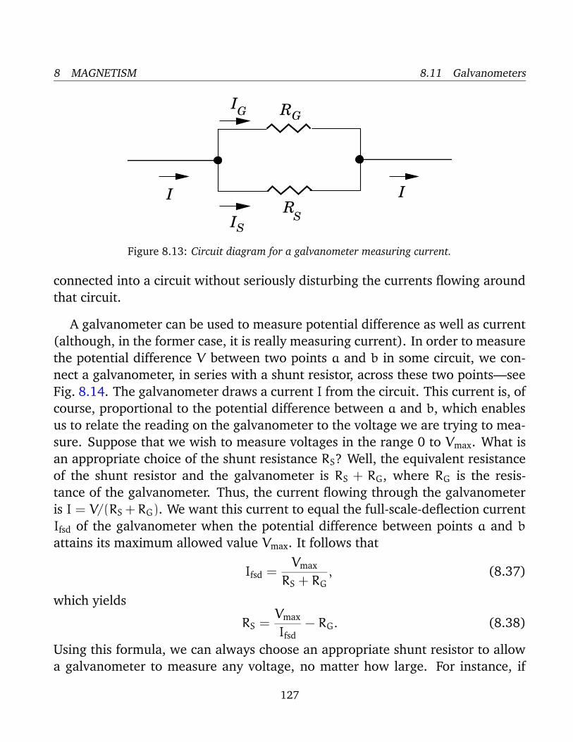
8 MAGNETISM 8.11 Galvanometers
I
I
I
I
G
S
RS
RG
Figure 8.13: Circuit diagram for a galvanometer measuring current.
connected into a circuit without seriously disturbing the currents flowing around
that circuit.
A galvanometer can be used to measure potential difference as well as current
(although, in the former case, it is really measuring current). In order to measure
the potential difference V between two points a and b in some circuit, we con-
nect a galvanometer, in series with a shunt resistor, across these two points—see
Fig. 8.14. The galvanometer draws a current I from the circuit. This current is, of
course, proportional to the potential difference between a and b, which enables
us to relate the reading on the galvanometer to the voltage we are trying to mea-
sure. Suppose that we wish to measure voltages in the range 0 to Vmax. What is
an appropriate choice of the shunt resistance RS? Well, the equivalent resistance
of the shunt resistor and the galvanometer is RS + RG, where RG is the resis-
tance of the galvanometer. Thus, the current flowing through the galvanometer
is I = V/(RS + RG). We want this current to equal the full-scale-deflection current
Ifsd of the galvanometer when the potential difference between points a and b
attains its maximum allowed value Vmax. It follows that
Ifsd =Vmax
RS + RG
, (8.37)
which yields
RS =Vmax
Ifsd
− RG. (8.38)
Using this formula, we can always choose an appropriate shunt resistor to allow
a galvanometer to measure any voltage, no matter how large. For instance, if
127
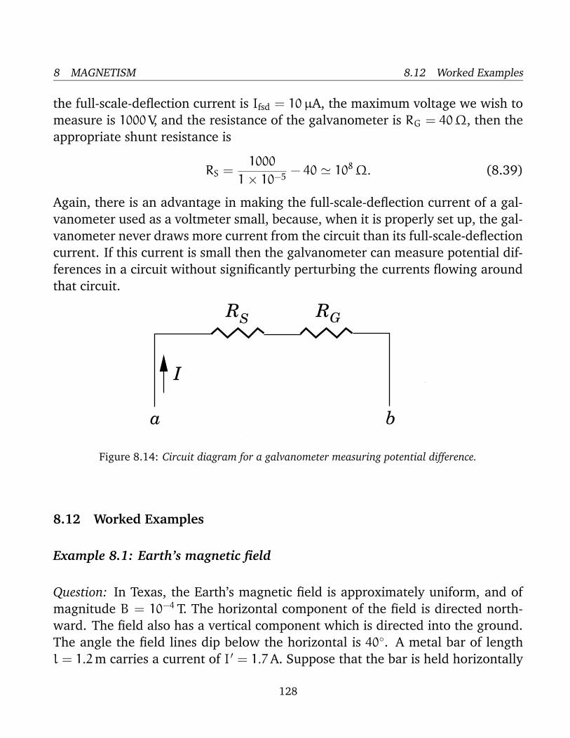
8 MAGNETISM 8.12 Worked Examples
the full-scale-deflection current is Ifsd = 10 µA, the maximum voltage we wish to
measure is 1000 V, and the resistance of the galvanometer is RG = 40 Ω, then the
appropriate shunt resistance is
RS =1000
1 × 10⁻⁵− 40 ' 108 Ω. (8.39)
Again, there is an advantage in making the full-scale-deflection current of a gal-
vanometer used as a voltmeter small, because, when it is properly set up, the gal-
vanometer never draws more current from the circuit than its full-scale-deflection
current. If this current is small then the galvanometer can measure potential dif-
ferences in a circuit without significantly perturbing the currents flowing around
that circuit.
.
.
GRS
I
a b
R
Figure 8.14: Circuit diagram for a galvanometer measuring potential difference.
8.12 Worked Examples
Example 8.1: Earth’s magnetic field
Question: In Texas, the Earth’s magnetic field is approximately uniform, and of
magnitude B = 10−4 T. The horizontal component of the field is directed north-
ward. The field also has a vertical component which is directed into the ground.
The angle the field lines dip below the horizontal is 40. A metal bar of length
l = 1.2 m carries a current of I ′ = 1.7 A. Suppose that the bar is held horizontally
128

8 MAGNETISM 8.12 Worked Examples
40o
ground
north
magnetic field lines
.
such that the current flows from East to West. What is the magnitude and direc-
tion of the magnetic force on the bar? Suppose that the direction of the current
is reversed. What, now, is the magnitude and direction of the magnetic force on
the bar? Suppose that the bar is held vertically such the current flows upward.
What is the magnitude and direction of the magnetic force on the bar? Suppose,
finally, that the direction of the current is reversed. What, now, is the magnitude
and direction of the magnetic force on the bar?
Answer: If the current in the bar flows horizontally from East to West then the
direction of the current makes an angle of 90 with the direction of the magnetic
field. So, from Eq. (8.1), the magnetic force per unit length acting on the bar is
F = I ′ B sin 90 = I ′ B = (1.7) (10−4) = 1.7 × 10⁻⁴ N m−1.
Thus, the total force acting on the bar is
f = F l = (1.7 × 10⁻⁴) (1.2) = 2.04 × 10⁻⁴ N.
Using the right-hand rule, if the index finger of a right-hand points horizontally
from East to West, and the middle finger points northward, but dips 40 below the
horizontal, then the thumb points southward, but dips 50 below the horizontal.
Thus, the force on the bar is directed southward, and dips 50 below the horizon-
tal. If the current in the bar is reversed, so that it now flows horizontally from
West to East, then the angle subtended between the direction of current flow and
the direction of the magnetic field is still 90, so the magnitude of the force on the
129

8 MAGNETISM 8.12 Worked Examples
bar remains unchanged. According to the right-hand rule, if the index finger of
a right-hand points horizontally from West to East, and the middle finger points
northward, but dips 40 below the horizontal, then the thumb points northward,
but is directed 50 above the horizontal. Thus, the force on the bar is directed
northward at an angle of 50 above the horizontal. In other words, the new force
points in exactly the opposite direction to the old one.
If the current in the bar flows vertically upward then the direction of current
flow subtends an angle of 50 degrees with the direction of the magnetic field.
So, from Eq. (8.1), the magnetic force per unit length acting on the bar is
F = I ′ B sin 50 = (1.7) (10−4) (0.7660) = 1.30 × 10⁻⁴ N m−1.
Thus, the total force acting on the bar is
f = F l = (1.30 × 10⁻⁴) (1.2) = 1.56 × 10⁻⁴ N.
Using the right-hand rule, if the index finger of a right-hand points vertically
upward, and the middle finger points northward, but dips 40 below the hori-
zontal, then the thumb points horizontally westward. Thus, the force on the bar
is directed horizontally westward. If the current in the bar is reversed, so that
it flows vertically downward, then the force on the bar is of the same magni-
tude, but points in the opposite direction, which means that the new force points
horizontally eastward.
Example 8.2: Charged particle in magnetic field
Question: Suppose that an electron is accelerated from rest through a voltage
difference of V = 103 volts and then passes into a region containing a uniform
magnetic field of magnitude B = 1.2 T. The electron subsequently executes a
closed circular orbit in the plane perpendicular to the field. What is the radius of
this orbit? What is the angular frequency of gyration of the electron?
Answer: If an electron of mass me = 9.11×10⁻³¹ kg and charge e = 1.60×10⁻¹⁹ C
is accelerated from rest through a potential difference V then its final kinetic
130

8 MAGNETISM 8.12 Worked Examples
energy is1
2me v2 = e V.
Thus, the final velocity v of the electron is given by
v =
√
√
√
√
2 e V
me
=
√
√
√
√
√
(2) (1.6 × 10⁻¹⁹) (103)
(9.11 × 10⁻³¹)= 1.87 × 10⁷ m s−1.
The initial direction of motion of the electron is at right-angles to the direction of
the magnetic field, otherwise the orbit of the electron would be a spiral instead
of a closed circle. Thus, we can use Eq. (8.16) to calculate the radius ρ of the
orbit. We obtain
ρ =me v
e B=
(9.11 × 10⁻³¹) (1.87 × 10⁷)
(1.6 × 10⁻¹⁹) (1.2)= 8.87 × 10⁻⁵ m.
The angular frequency of gyration ω of the electron comes from Eq. (8.17):
ω =e B
me
=(1.6 × 10⁻¹⁹) (1.2)
(9.11 × 10⁻³¹)= 2.11 × 10¹¹ rad. s−1
.
Example 8.3: Ampere’s circuital law
Question: A z-directed wire of radius a carries a total z-directed current I. What
is the magnetic field distribution, both inside and outside the wire, if the current
is evenly distributed throughout the wire? What is the magnetic field distribution
if the current is concentrated in a thin layer at the surface of the wire?
Answer: Since the current distribution possesses cylindrical symmetry, it is rea-
sonable to suppose that the magnetic field it generates also possesses cylindrical
symmetry. By analogy with the magnetic field generated by an infinitely thin z-
directed wire, we expect the magnetic field to circulate in the x-y plane in an
anti-clockwise direction (looking against the direction of the current). Let us ap-
ply Ampere’s circuital law to a circular loop in the x-y plane which is centred
on the centre of the wire, and is of radius r > a. The magnetic field is every-
where tangential to the loop, so the line integral of the magnetic field (taken in
131

8 MAGNETISM 8.12 Worked Examples
an anti-clockwise sense, looking against the direction of the current) is
w(r) = 2π r B(r),
where B(r) is the magnetic field-strength at radius r. According to Ampere’s
circuital law, this line integral is equal to µ0 times the total current enclosed by
the loop. The total current is clearly I, since the loop lies outside the wire. Thus,
w(r) = 2π r B(r) = µ0 I,
giving
B(r) =µ0 I
2π r
for r > a. This is exactly the same field distribution as that generated by an
infinitely thin wire carrying the current I. Thus, we conclude that the magnetic
field generated outside a cylindrically symmetric z-directed current distribution
is the same as if all of the current were concentrated at the centre of the distri-
bution. Let us now apply Ampere’s circuital law to a circular loop which is of
radius r < a. The line integral of the magnetic field around this loop is simply
w(r) = 2π r B(r). However, the current enclosed by the loop is equal to I times
the ratio of the area of the loop to the cross-sectional area of the wire (since the
current is evenly distributed throughout the wire). Thus, Ampere’s law yields
2π r B(r) = µ0 Ir2
a2,
which gives
B(r) =µ0 I r
2π a2.
Clearly, the field inside the wire increases linearly with increasing distance from
the centre of the wire.
If the current flows along the outside of the wire then the magnetic field distri-
bution exterior to the wire is exactly the same as that described above. However,
there is no field inside the wire. This follows immediately from Ampere’s circuital
law because the current enclosed by a circular loop whose radius is less than the
radius of the wire is clearly zero.
132

9 MAGNETIC INDUCTION
9 Magnetic Induction
9.1 Faraday’s Law
The phenomenon of magnetic induction plays a crucial role in three very useful
electrical devices: the electric generator, the electric motor, and the transformer.
Without these devices, modern life would be impossible in its present form. Mag-
netic induction was discovered in 1830 by the English physicist Michael Faraday.
The American physicist Joseph Henry independently made the same discovery
at about the same time. Both physicists were intrigued by the fact that an elec-
tric current flowing around a circuit can generate a magnetic field. Surely, they
reasoned, if an electric current can generate a magnetic field then a magnetic
field must somehow be able to generate an electric current. However, it took
many years of fruitless experimentation before they were able to find the essen-
tial ingredient which allows a magnetic field to generate an electric current. This
ingredient is time variation.
Consider a planar loop C of conducting wire of cross-sectional area A. Let us
place this loop in a magnetic field whose strength B is approximately uniform
over the extent of the loop. Suppose that the direction of the magnetic field
subtends an angle θ with the normal direction to the loop. The magnetic flux
ΦB through the loop is defined as the product of the area of the loop and the
component of the magnetic field perpendicular to the loop. Thus,
ΦB = A B⊥ = A B cos θ. (9.1)
If the loop is wrapped around itself N times (i.e., if the loop has N turns) then
the magnetic flux through the loop is simply N times the magnetic flux through
a single turn:
ΦB = N A B⊥. (9.2)
Finally, if the magnetic field is not uniform over the loop, or the loop does not lie
in one plane, then we must evaluate the magnetic flux as a surface integral
ΦB =
∫
S
B · dS. (9.3)
133

9 MAGNETIC INDUCTION 9.1 Faraday’s Law
Here, S is some surface attached to C. If the loop has N turns then the flux is N
times the above value. The SI unit of magnetic flux is the weber (Wb). One tesla
is equivalent to one weber per meter squared:
1 T ≡ 1 Wb m−2. (9.4)
Faraday discovered that if the magnetic field through a loop of wire varies in
time then an emf is induced around the loop. Faraday was able to observe this
effect because the emf gives rise to a current circulating in the loop. Faraday
found that the magnitude of the emf is directly proportional to the time rate of
change of the magnetic field. He also discovered that an emf is generated when
a loop of wire moves from a region of low magnetic field-strength to one of high
magnetic field-strength, and vice versa. The emf is directly proportional to the
velocity with which the loop moves between the two regions. Finally, Faraday
discovered that an emf is generated around a loop which rotates in a uniform
magnetic field of constant strength. In this case, the emf is directly proportional
to the rate at which the loop rotates. Faraday was eventually able to propose a
single law which could account for all of his many and varied observations. This
law, which is known as Faraday’s law of magnetic induction, is as follows:
The emf induced in a circuit is proportional to the time rate of change of the
magnetic flux linking that circuit.
SI units have been fixed so that the constant of proportionality in this law is unity.
Thus, if the magnetic flux through a circuit changes by an amount dΦB in a time
interval dt then the emf E generated in the circuit is
E =dΦB
dt. (9.5)
There are many different ways in which the magnetic flux linking an electric
circuit can change. Either the magnetic field-strength can change, or the direction
of the magnetic field can change, or the position of the circuit can change, or the
shape of the circuit can change, or the orientation of the circuit can change.
Faraday’s law states that all of these ways are completely equivalent as far as the
generation of an emf around the circuit is concerned.
134

9 MAGNETIC INDUCTION 9.2 Lenz’s Law
magnetic field lines
conducting loop
I
Figure 9.1: Magnetic field generated by a planar current-carrying loop.
9.2 Lenz’s Law
We still have not specified in which direction the emf generated by a time-varying
magnetic flux linking an electric circuit acts. In order to help specify this direc-
tion, we need to make use of a right-hand rule. Suppose that a current I circulates
around a planar loop of conducting wire, and, thereby, generates a magnetic field
B. What is the direction of this magnetic field as it passes through the middle of
the loop? Well, if the fingers of a right-hand circulate in the same direction as the
current, then the thumb indicates the direction of the magnetic field as it passes
through the centre of the loop. This is illustrated in Fig. 9.1.
Consider a plane loop of conducting wire which is linked by magnetic flux.
By convention, the direction in which current would have to flow around the
loop in order to increase the magnetic flux linking the loop is termed the positive
direction. Likewise, the direction in which current would have to flow around
the loop in order to decrease the magnetic flux linking the loop is termed the
negative direction. Suppose that the magnetic flux linking the loop is increased.
In accordance with Faraday’s law, an emf is generated around the loop. Does this
emf act in the positive direction, so as to drive a current around the loop which
further increases the magnetic flux, or does it act in the negative direction, so as
135

9 MAGNETIC INDUCTION 9.3 Magnetic Induction
to drive a current around the loop which decreases the magnetic flux? It is easily
demonstrated experimentally that the emf acts in the negative direction. Thus:
The emf induced in an electric circuit always acts in such a direction that
the current it drives around the circuit opposes the change in magnetic flux
which produces the emf.
This result is known as Lenz’s law, after the nineteenth century Russian scientist
Heinrich Lenz, who first formulated it. Faraday’s law, combined with Lenz’s law,
is usually written
E = −dΦB
dt. (9.6)
The minus sign is to remind us that the emf always acts to oppose the change in
magnetic flux which generates the emf.
9.3 Magnetic Induction
Consider a one-turn loop of conducting wire C which is placed in a magnetic field
B. The magnetic flux ΦB linking loop C can be written
ΦB =
∫
S
B · dS (9.7)
where S is any surface attached to the loop.
Suppose that the magnetic field changes in time, causing the magnetic flux
ΦB linking circuit C to vary. Let the flux change by an amount dΦB in the time
interval dt. According to Faraday’s law, the emf E induced around loop C is given
by
E = −dΦB
dt. (9.8)
If E is positive then the emf acts around the loop in the same sense as that indi-
cated by the fingers of a right-hand, when the thumb points in the direction of
the mean magnetic field passing through the loop. Likewise, if E is negative then
the emf acts around the loop in the opposite sense to that indicated by the fingers
136

9 MAGNETIC INDUCTION 9.3 Magnetic Induction
of a right-hand, when the thumb points in the direction of the mean magnetic
field passing through the loop. In the former case, we say that the emf acts in
the positive direction, whereas in the latter case we say it acts in the negative
direction.
Suppose that E > 0, so that the emf acts in the positive direction. How, ex-
actly, is this emf produced? In order to answer this question, we need to remind
ourselves what an emf actually is. When we say that an emf E acts around the
loop C in the positive direction, what we really mean is that a charge q which
circulates once around the loop in the positive direction acquires the energy q E .
How does the charge acquire this energy? Clearly, either an electric field or a
magnetic field, or some combination of the two, must perform the work q E on
the charge as it circulates around the loop. However, we have already seen, from
Sect. 8.4, that a magnetic field is unable to do work on a charged particle. Thus,
the charge must acquire the energy q E from an electric field as it circulates once
around the loop in the positive direction.
According to Sect. 5, the work that the electric field does on the charge as it
goes around the loop is
W = q
∮
C
E · dr, (9.9)
where dr is a line element of the loop. Hence, by energy conservation, we can
write W = q E , or
E =
∮
C
E · dr. (9.10)
The term on the right-hand side of the above expression can be recognized as the
line integral of the electric field around loop C in the positive direction. Thus, the
emf generated around the circuit C in the positive direction is equal to the line
integral of the electric field around the circuit in the same direction.
Equations (9.8) and (9.10) can be combined to give∮
C
E · dr = −dΦB
dt. (9.11)
Thus, Faraday’s law implies that the line integral of the electric field around cir-
cuit C (in the positive direction) is equal to minus the time rate of change of the
137

9 MAGNETIC INDUCTION 9.3 Magnetic Induction
magnetic flux linking this circuit. Does this law just apply to conducting circuits,
or can we apply it to an arbitrary closed loop in space? Well, the difference be-
tween a conducting circuit and an arbitrary closed loop is that electric current
can flow around a circuit, whereas current cannot, in general, flow around an
arbitrary loop. In fact, the emf E induced around a conducting circuit drives a
current I = E/R around that circuit, where R is the resistance of the circuit. How-
ever, we can make this resistance arbitrarily large without invalidating Eq. (9.11).
In the limit in which R tends to infinity, no current flows around the circuit, so
the circuit becomes indistinguishable from an arbitrary loop. Since we can place
such a circuit anywhere in space, and Eq. (9.11) still holds, we are forced to the
conclusion that Eq. (9.11) is valid for any closed loop in space, and not just for
conducting circuits.
Equation (9.11) describes how a time-varying magnetic field generates an elec-
tric field which fills space. The strength of the electric field is directly proportional
to the rate of change of the magnetic field. The field-lines associated with this
electric field form loops in the plane perpendicular to the magnetic field. If the
magnetic field is increasing then the electric field-lines circulate in the opposite
sense to the fingers of a right-hand, when the thumb points in the direction of
the field. If the magnetic field is decreasing then the electric field-lines circulate
in the same sense as the fingers of a right-hand, when the thumb points in the
direction of the field. This is illustrated in Fig. 9.2.
We can now appreciate that when a conducting circuit is placed in a time-
varying magnetic field, it is the electric field induced by the changing magnetic
field which gives rise to the emf around the circuit. If the loop has a finite re-
sistance then this electric field also drives a current around the circuit. Note,
however, that the electric field is generated irrespective of the presence of a con-
ducting circuit. The electric field generated by a time-varying magnetic field is
quite different in nature to that generated by a set of stationary electric charges.
In the latter case, the electric field-lines begin on positive charges, end on nega-
tive charges, and never form closed loops in free space. In the former case, the
electric field-lines never begin or end, and always form closed loops in free space.
In fact, the electric field-lines generated by magnetic induction behave in much
the same manner as magnetic field-lines. Recall, from Sect. 5.1, that an elec-
138

9 MAGNETIC INDUCTION 9.3 Magnetic Induction
increasing magnetic field
E
B
E
B
decreasing magnetic field
Figure 9.2: Inductively generated electric fields
.
tric field generated by fixed charges is unable to do net work on a charge which
circulates in a closed loop. On the other hand, an electric field generated by mag-
netic induction certainly can do work on a charge which circulates in a closed
loop. This is basically how a current is induced in a conducting loop placed in a
time-varying magnetic field. One consequence of this fact is that the work done
in slowly moving a charge between two points in an inductive electric field does
depend on the path taken between the two points. It follows that we cannot cal-
culate a unique potential difference between two points in an inductive electric
field. In fact, the whole idea of electric potential breaks down in a such a field
(fortunately, there is a way of salvaging the idea of electric potential in an in-
ductive field, but this topic lies beyond the scope of this course). Note, however,
that it is still possible to calculate a unique value for the emf generated around
a conducting circuit by an inductive electric field, because, in this case, the path
taken by electric charges is uniquely specified: i.e., the charges have to follow the
circuit.
139

9 MAGNETIC INDUCTION 9.4 Motional Emf
rod frame
l
I
I
v
magnetic field into page
B
x
Figure 9.3: Motional emf.
9.4 Motional Emf
We now understand how an emf is generated around a fixed circuit placed in
a time-varying magnetic field. But, according to Faraday’s law, an emf is also
generated around a moving circuit placed in a magnetic field which does not
vary in time. According to Eq. (9.11), no space-filling inductive electric field is
generated in the latter case, since the magnetic field is steady. So, how do we
account for the emf in the latter case?
In order to help answer this question, let us consider a simple circuit in which
a conducting rod of length l slides along a U-shaped conducting frame in the
presence of a uniform magnetic field. This circuit is illustrated in Fig. 9.3. Sup-
pose, for the sake of simplicity, that the magnetic field is directed perpendicular
to the plane of the circuit. To be more exact, the magnetic field is directed into
the page in the figure. Suppose, further, that we move the rod to the right with
the constant velocity v.
The magnetic flux linked by the circuit is simply the product of the perpendicu-
lar magnetic field-strength, B, and the area of the circuit, l x, where x determines
140

9 MAGNETIC INDUCTION 9.4 Motional Emf
the position of the sliding rod. Thus,
ΦB = B l x. (9.12)
Now, the rod moves a distance dx = v dt in a time interval dt, so in the same
time interval the magnetic flux linking the circuit increases by
dΦB = B l dx = B l v dt. (9.13)
It follows, from Faraday’s law, that the magnitude of the emf E generated around
the circuit is given by
E =dΦB
dt= B l v. (9.14)
Thus, the emf generated in the circuit by the moving rod is simply the product
of the magnetic field-strength, the length of the rod, and the velocity of the rod.
If the magnetic field is not perpendicular to the circuit, but instead subtends an
angle θ with respect to the normal direction to the plane of the circuit, then it is
easily demonstrated that the motional emf generated in the circuit by the moving
rod is
E = B⊥ l v, (9.15)
where B⊥ = B cos θ is the component of the magnetic field which is perpendicu-
lar to the plane of the circuit.
Since the magnetic flux linking the circuit increases in time, the emf acts in the
negative direction (i.e., in the opposite sense to the fingers of a right-hand, if the
thumb points along the direction of the magnetic field). The emf, E , therefore,
acts in the anti-clockwise direction in the figure. If R is the total resistance of
the circuit, then this emf drives an anti-clockwise electric current of magnitude
I = E/R around the circuit.
But, where does the emf come from? Let us again remind ourselves what an
emf is. When we say that an emf E acts around the circuit in the anti-clockwise
direction, what we really mean is that a charge q which circulates once around
the circuit in the anti-clockwise direction acquires the energy q E . The only way
in which the charge can acquire this energy is if something does work on it as
it circulates. Let us assume that the charge circulates very slowly. The magnetic
141

9 MAGNETIC INDUCTION 9.4 Motional Emf
field exerts a negligibly small force on the charge when it is traversing the non-
moving part of the circuit (since the charge is moving very slowly). However,
when the charge is traversing the moving rod it experiences an upward (in the
figure) magnetic force of magnitude f = q v B (assuming that q > 0). The net
work done on the charge by this force as it traverses the rod is
W ′ = q v B l = q E , (9.16)
since E = B l v. Thus, it would appear that the motional emf generated around
the circuit can be accounted for in terms of the magnetic force exerted on charges
traversing the moving rod.
But, if we think carefully, we can see that there is something seriously wrong
with the above explanation. We seem to be saying that the charge acquires the
energy q E from the magnetic field as it moves around the circuit once in the anti-
clockwise direction. But, this is impossible, because a magnetic field cannot do
work on an electric charge.
Let us look at the problem from the point of view of a charge q traversing the
moving rod. In the frame of reference of the rod, the charge only moves very
slowly, so the magnetic force on it is negligible. In fact, only an electric field can
exert a significant force on a slowly moving charge. In order to account for the
motional emf generated around the circuit, we need the charge to experience an
upward force of magnitude q v B. The only way in which this is possible is if the
charge sees an upward pointing electric field of magnitude
E0 = v B. (9.17)
In other words, although there is no electric field in the laboratory frame, there
is an electric field in the frame of reference of the moving rod, and it is this field
which does the necessary amount of work on charges moving around the circuit
to account for the existence of the motional emf, E = B l v.
More generally, if a conductor moves in the laboratory frame with velocity
v in the presence of a magnetic field B then a charge q inside the conductor
experiences a magnetic force f = q v×B. In the frame of the conductor, in which
the charge is essentially stationary, the same force takes the form of an electric
142

9 MAGNETIC INDUCTION 9.5 Eddy Currents
force f = q E0, where E0 is the electric field in the frame of reference of the
conductor. Thus, if a conductor moves with velocity v through a magnetic field B
then the electric field E0 which appears in the rest frame of the conductor is given
by
E0 = v × B. (9.18)
This electric field is the ultimate origin of the motional emfs which are generated
whenever circuits move with respect to magnetic fields.
We can now appreciate that Faraday’s law is due to a combination of two
apparently distinct effects. The first is the space-filling electric field generated
by a changing magnetic field. The second is the electric field generated inside a
conductor when it moves through a magnetic field. In reality, these effects are two
aspects of the same basic phenomenon, which explains why no real distinction is
made between them in Faraday’s law.
9.5 Eddy Currents
We have seen, in the above example, that when a conductor is moved in a mag-
netic field a motional emf is generated. Moreover, according to Worked Example
9.3, this emf drives a current which heats the conductor, and, when combined
with the magnetic field, also gives rise to a magnetic force acting on the conduc-
tor which opposes its motion. In turns out that these results are quite general.
Incidentally, the induced currents which circulate inside a moving conductor in a
static magnetic field, or a stationary conductor in a time-varying magnetic field,
are usually called eddy currents.
Consider a metal disk which rotates in a perpendicular magnetic field which
only extends over a small rectangular portion of the disk, as shown in Fig. 9.4.
Such a field could be produced by the pole of a horseshoe magnetic. The motional
emf induced in the disk, as it moves through the field-containing region, acts in
the direction v×B, where v is the velocity of the disk, and B the magnetic field. It
follows from Fig. 9.4 that the emf acts downward. The emf drives currents which
are also directed downward. However, these currents must form closed loops,
and, hence, they are directed upward in those regions of the disk immediately
143

9 MAGNETIC INDUCTION 9.5 Eddy Currents
eddy current
direction of rotation of metal disk
magnetic fieldinto page
Figure 9.4: Eddy currents
.
adjacent to the field-containing region, as shown in the figure. It can be seen
that the induced currents flow in little eddies. Hence, the name “eddy currents.”
According to the right-hand rule, the downward currents in the field-containing
region give rise to a magnetic force on the disk which acts to the right. In other
words, the magnetic force acts to prevent the rotation of the disk. Clearly, ex-
ternal work must be done on the disk in order to keep it rotating at a constant
angular velocity. This external work is ultimately dissipated as heat by the eddy
currents circulating inside the disk.
Eddy currents can be very useful. For instance, some cookers work by using
eddy currents. The cooking pots, which are usually made out of aluminium, are
placed on plates which generate oscillating magnetic fields. These fields induce
eddy currents in the pots which heat them up. The heat is then transmitted to
the food inside the pots. This type of cooker is particularly useful for food which
needs to be cooked gradually over a long period of time: i.e., over many hours, or
even days. Eddy currents can also be used to heat small pieces of metal until they
become white-hot by placing them in a very rapidly oscillating magnetic field.
This technique is sometimes used in brazing. Heating conductors by means of
eddy currents is called inductive heating. Eddy currents can also be used to damp
144

9 MAGNETIC INDUCTION 9.6 The Alternating Current Generator
l
w
axis of rotation rotating coil
magnetic field
side view
coil
v
v
direction of magnetic field
direction of rotation
end view
θ
a b
d c
Figure 9.5: An alternating current generator.
motion. This technique, which is called eddy current damping, is often employed
in galvanometers.
9.6 The Alternating Current Generator
An electric generator, or dynamo, is a device which converts mechanical energy
into electrical energy. The simplest practical generator consists of a rectangular
coil rotating in a uniform magnetic field. The magnetic field is usually supplied
by a permanent magnet. This setup is illustrated in Fig. 9.5.
Let l be the length of the coil along its axis of rotation, and w the width of
the coil perpendicular to this axis. Suppose that the coil rotates with constant
angular velocity ω in a uniform magnetic field of strength B. The velocity v with
which the the two long sides of the coil (i.e., sides ab and cd) move through the
magnetic field is simply the product of the angular velocity of rotation ω and the
distance w/2 of each side from the axis of rotation, so v = ω w/2. The motional
emf induced in each side is given by E = B⊥ l v, where B⊥ is the component of
the magnetic field perpendicular to instantaneous direction of motion of the side
in question. If the direction of the magnetic field subtends an angle θ with the
145

9 MAGNETIC INDUCTION 9.6 The Alternating Current Generator
normal direction to the coil, as shown in the figure, then B⊥ = B sin θ. Thus, the
magnitude of the motional emf generated in sides ab and cd is
Eab =B w l ω sin θ
2=
B A ω sin θ
2, (9.19)
where A = w l is the area of the coil. The emf is zero when θ = 0 or 180,since the direction of motion of sides ab and cd is parallel to the direction of
the magnetic field in these cases. The emf attains its maximum value when θ =
90 or 270, since the direction of motion of sides ab and cd is perpendicular to
the direction of the magnetic field in these cases. Incidentally, it is clear, from
symmetry, that no net motional emf is generated in sides bc and da of the coil.
Suppose that the direction of rotation of the coil is such that side ab is moving
into the page in Fig. 9.5 (side view), whereas side cd is moving out of the page.
The motional emf induced in side ab acts from a to b. Likewise, the motional
emf induce in side cd acts from c to d. It can be seen that both emfs act in the
clockwise direction around the coil. Thus, the net emf E acting around the coil is
2 Eab. If the coil has N turns then the net emf becomes 2 N Eab. Thus, the general
expression for the emf generated around a steadily rotating, multi-turn coil in a
uniform magnetic field is
E = N B A ω sin(ω t), (9.20)
where we have written θ = ω t for a steadily rotating coil (assuming that θ = 0
at t = 0). This expression can also be written
E = Emax sin(2π f t), (9.21)
where
Emax = 2π N B A f (9.22)
is the peak emf produced by the generator, and f = ω/2π is the number of
complete rotations the coils executes per second. Thus, the peak emf is directly
proportional to the area of the coil, the number of turns in the coil, the rotation
frequency of the coil, and the magnetic field-strength.
Figure 9.6 shows the emf specified in Eq. (9.21) plotted as a function of time.
It can be seen that the variation of the emf with time is sinusoidal in nature. The
146

9 MAGNETIC INDUCTION 9.6 The Alternating Current Generator
.
.
εmax
ε
t −>0
T = 1/f
−>
Figure 9.6: Emf generated by a steadily rotating AC generator.
emf attains its peak values when the plane of the coil is parallel to the plane of the
magnetic field, passes through zero when the plane of the coil is perpendicular to
the magnetic field, and reverses sign every half period of revolution of the coil.
The emf is periodic (i.e., it continually repeats the same pattern in time), with
period T = 1/f (which is, of course, the rotation period of the coil).
Suppose that some load (e.g., a light-bulb, or an electric heating element) of
resistance R is connected across the terminals of the generator. In practice, this is
achieved by connecting the two ends of the coil to rotating rings which are then
connected to the external circuit by means of metal brushes. According to Ohm’s
law, the current I which flows in the load is given by
I =ER
=Emax
Rsin(2π f t). (9.23)
Note that this current is constantly changing direction, just like the emf of the
generator. Hence, the type of generator described above is usually termed an
alternating current, or AC, generator.
The current I which flows through the load must also flow around the coil.
Since the coil is situated in a magnetic field, this current gives rise to a torque on
the coil which, as is easily demonstrated, acts to slow down its rotation. Accord-
ing to Sect. 8.11, the braking torque τ acting on the coil is given by
τ = N I B‖ A, (9.24)
147

9 MAGNETIC INDUCTION 9.6 The Alternating Current Generator
where B‖ = B sin θ is the component of the magnetic field which lies in the plane
of the coil. It follows from Eq. (9.20) that
τ =E I
ω, (9.25)
since E = N B‖ A ω. An external torque which is equal and opposite to the break-
ing torque must be applied to the coil if it is to rotate uniformly, as assumed
above. The rate P at which this external torque does work is equal to the product
of the torque τ and the angular velocity ω of the coil. Thus,
P = τ ω = E I. (9.26)
Not surprisingly, the rate at which the external torque performs works exactly
matches the rate E I at which electrical energy is generated in the circuit com-
prising the rotating coil and the load.
Equations (9.20), (9.23), and (9.25) yield
τ = τmax sin2(2π f t), (9.27)
where τmax = (Emax)2/(2π f R). Figure 9.7 shows the breaking torque τ plotted
as a function of time t, according to Eq. (9.27). It can be seen that the torque
is always of the same sign (i.e., it always acts in the same direction, so as to
continually oppose the rotation of the coil), but is not constant in time. Instead,
it pulsates periodically with period T . The breaking torque attains its maximum
value whenever the plane of the coil is parallel to the plane of the magnetic
field, and is zero whenever the plane of the coil is perpendicular to the magnetic
field. It is clear that the external torque needed to keep the coil rotating at a
constant angular velocity must also pulsate in time with period T . A constant
external torque would give rise to a non-uniformly rotating coil, and, hence, to
an alternating emf which varies with time in a more complicated manner than
sin(2π f t).
Virtually all commercial power stations generate electricity using AC genera-
tors. The external power needed to turn the generating coil is usually supplied
by a steam turbine (steam blasting against fan-like blades which are forced into
rotation). Water is vaporized to produce high pressure steam by burning coal, or
148

9 MAGNETIC INDUCTION 9.7 The Direct Current Generator
.
.t −>0
T = 1/f
max
−>
τ
τ
Figure 9.7: The braking torque in a steadily rotating AC generator.
by using the energy released inside a nuclear reactor. Of course, in hydroelectric
power stations, the power needed to turn the generator coil is supplied by a water
turbine (which is similar to a steam turbine, except that falling water plays the
role of the steam). Recently, a new type of power station has been developed in
which the power needed to rotate the generating coil is supplied by a gas turbine
(basically, a large jet engine which burns natural gas). In the United States and
Canada, the alternating emf generated by power stations oscillates at f = 60 Hz,
which means that the generator coils in power stations rotate exactly sixty times
a second. In Europe, and much of the rest of the world, the oscillation frequency
of commercially generated electricity is f = 50 Hz.
9.7 The Direct Current Generator
Most common electrical appliances (e.g., electric light-bulbs, and electric heating
elements) work fine on AC electrical power. However, there are some situations
in which DC power is preferable. For instance, small electric motors (e.g., those
which power food mixers and vacuum cleaners) work very well on AC electricity,
but very large electric motors (e.g., those which power subway trains) generally
work much better on DC electricity. Let us investigate how DC electricity can be
generated.
149

9 MAGNETIC INDUCTION 9.7 The Direct Current Generator
rotating split−ring
lead to external circuit
metal brush
Figure 9.8: A split-ring commutator.
A simple DC generator consists of the same basic elements as a simple AC gen-
erator: i.e., a multi-turn coil rotating uniformly in a magnetic field. The main
difference between a DC generator and an AC generator lies in the manner in
which the rotating coil is connected to the external circuit containing the load. In
an AC generator, both ends of the coil are connected to separate slip-rings which
co-rotate with the coil, and are connected to the external circuit via wire brushes.
In this manner, the emf Eext seen by the external circuit is always the same as
the emf E generated around the rotating coil. In a DC generator, the two ends
of the coil are attached to different halves of a single split-ring which co-rotates
with the coil. The split-ring is connected to the external circuit by means of metal
brushes—see Fig. 9.8. This combination of a rotating split-ring and stationary
metal brushes is called a commutator. The purpose of the commutator is to en-
sure that the emf Eext seen by the external circuit is equal to the emf E generated
around the rotating coil for half the rotation period, but is equal to minus this
emf for the other half (since the connection between the external circuit and the
rotating coil is reversed by the commutator every half-period of rotation). The
positions of the metal brushes can be adjusted such that the connection between
the rotating coil and the external circuit reverses whenever the emf E generated
around the coil goes through zero. In this special case, the emf seen in the exter-
nal circuit is simply
Eext = |E | = Emax | sin(2π f t)|. (9.28)
150

9 MAGNETIC INDUCTION 9.8 The Alternating Current Motor
.
.t −>0
T = 1/f
maxε
ε ext−
>
Figure 9.9: Emf generated in a steadily rotating DC generator.
Figure 9.9 shows Eext plotted as a function of time, according to the above for-
mula. The variation of the emf with time is very similar to that of an AC generator,
except that whenever the AC generator would produce a negative emf the com-
mutator in the DC generator reverses the polarity of the coil with respect to the
external circuit, so that the negative half of the AC signal is reversed and made
positive. The result is a bumpy direct emf which rises and falls but never changes
direction. This type of pulsating emf can be smoothed out by using more than
one coil rotating about the same axis, or by other electrical techniques, to give
a good imitation of the direct current delivered by a battery. The alternator in
a car (i.e., the DC generator which recharges the battery) is a common example
of a DC generator of the type discussed above. Of course, in an alternator, the
external torque needed to rotate the coil is provided by the engine of the car.
9.8 The Alternating Current Motor
The first electric dynamo was constructed in 1831 by Michael Faraday. An electric
dynamo is, of course, a device which transforms mechanical energy into electri-
cal energy. An electric motor, on the other hand, is a device which transforms
electrical energy into mechanical energy. In other words, an electric motor is an
electric dynamo run in reverse. It took a surprisingly long time for scientists in
151

9 MAGNETIC INDUCTION 9.8 The Alternating Current Motor
the nineteenth century to realize this. In fact, the message only really sank home
after a fortuitous accident during the 1873 Vienna World Exposition. A large hall
was filled with modern gadgets. One of these gadgets, a steam engine driven dy-
namo, was producing electric power when a workman unwittingly connected the
output leads from another dynamo to the energized circuit. Almost immediately,
the latter dynamo started to whirl around at great speed. The dynamo was, in
effect, transformed into an electric motor.
An AC electric motor consists of the same basic elements as an AC electric
generator: i.e., a multi-turn coil which is free to rotate in a constant magnetic
field. Furthermore, the rotating coil is connected to the external circuit in just
the same manner as in an AC generator: i.e., via two slip-rings attached to metal
brushes. Suppose that an external voltage source of emf V is connected across
the motor. It is assumed that V is an alternating emf, so that
V = Vmax sin(2π f t), (9.29)
where Vmax is the peak voltage, and f is the alternation frequency. Such an emf
could be obtained from an AC generator, or, more simply, from the domestic
mains supply. For the case of the mains, Vmax = 110 V and f = 60 Hz in the
U.S. and Canada, whereas Vmax = 220 V and f = 50 Hz in Europe and Asia. The
external emf drives an alternating current
I = Imax sin(2π f t) (9.30)
around the external circuit, and through the motor. As this current flows around
the coil, the magnetic field exerts a torque on the coil, which causes it to rotate.
The motor eventually attains a steady-state in which the rotation frequency of the
coil matches the alternation frequency of the external emf. In other words, the
steady-state rotation frequency of the coil is f. Now a coil rotating in a magnetic
field generates an emf E . It is easily demonstrated that this emf acts to oppose
the circulation of the current around the coil: i.e., the induced emf acts in the
opposite direction to the external emf. For an N-turn coil of cross-sectional area
A, rotating with frequency f in a magnetic field B, the back-emf E is given by
E = Emax sin(2π f t), (9.31)
152

9 MAGNETIC INDUCTION 9.8 The Alternating Current Motor
~
~
.
.
εR
VIexternal emf
internal resistance
motor
back-emf
Figure 9.10: Circuit diagram for an AC motor connected to an external AC emf source.
where
Emax = 2π N B A f, (9.32)
and use has been made of the results of Sect. 9.6.
Figure 9.10 shows the circuit in question. A circle with a wavy line inside is
the conventional way of indicating an AC voltage source. The motor is modeled
as a resistor R, which represents the internal resistance of the motor, in series
with the back-emf E . Of course, the back-emf acts in the opposite direction to the
external emf V . Application of Ohm’s law around the circuit gives
V = I R + E , (9.33)
or
Vmax sin(2π f t) = Imax R sin(2π f t) + Emax sin(2π f t), (9.34)
which reduces to
Vmax = Imax R + Emax. (9.35)
The rate P at which the motor gains electrical energy from the external circuit
is given by
P = E I = Pmax sin2(2π f t), (9.36)
153

9 MAGNETIC INDUCTION 9.9 The Direct Current Motor
where
Pmax = Emax Imax =Emax (Vmax − Emax)
R. (9.37)
By conservation of energy, P is also the rate at which the motor performs me-
chanical work. Note that the rate at which the motor does mechanical work is
not constant in time, but, instead, pulsates at the rotation frequency of the coil.
It is possible to construct a motor which performs work at a more uniform rate
by employing more than one coil rotating about the same axis.
As long as Vmax > Emax, the rate at which the motor performs mechanical work
is positive (i.e., the motor does useful work). However, if Vmax < Emax then the
rate at which the motor performs work becomes negative. This means that we
must do mechanical work on the motor in order to keep it rotating, which is
another way of saying that the motor does not do useful work. Clearly, in order
for an AC motor to do useful work, the external emf V must be able to overcome
the back-emf E induced in the motor (i.e., Vmax > Emax).
9.9 The Direct Current Motor
In steady-state, an AC motor always rotates at the alternation frequency of its
power supply. Thus, an AC motor powered by the domestic mains supply rotates
at 60 Hz in the U.S. and Canada, and at 50 Hz in Europe and Asia. Suppose,
however, that we require a variable speed electric motor. We could always use
an AC motor driven by a variable frequency AC power supply, but such power
supplies are very expensive. A far cheaper alternative is to use a DC motor driven
by a DC power supply. Let us investigate DC motors.
A DC motor consists of the same basic elements as a DC electric generator: i.e.,
a multi-turn coil which is free to rotate in a constant magnetic field. Furthermore,
the rotating coil is connected to the external circuit in just the same manner as in
a DC generator: i.e., via a split-ring commutator which reverses the polarity of the
coil with respect to the external circuit whenever the coil passes through the plane
perpendicular to the direction of the magnetic field. Suppose that an external DC
voltage source (e.g., a battery, or a DC generator) of emf V is connected across the
154

9 MAGNETIC INDUCTION 9.9 The Direct Current Motor
.
.
εR
VIexternal emf
internal resistance
motor
back-emf
Figure 9.11: Circuit diagram for an DC motor connected to an external DC emf source.
motor. The voltage source drives a steady current I around the external circuit,
and through the motor. As the current flows around the coil, the magnetic field
exerts a torque on the coil, which causes it to rotate. Let us suppose that the
motor eventually attains a steady-state rotation frequency f. The rotating coil
generates a back-emf E whose magnitude is directly proportional to the frequency
of rotation [see Eq. (9.32)].
Figure 9.11 shows the circuit in question. The motor is modeled as a resistor
R, which represents the internal resistance of the motor, in series with the back-
emf E . Of course, the back-emf acts in the opposite direction to the external emf
V . Application of Ohm’s law around the circuit gives
V = I R + E , (9.38)
which yields
I =V − E
R. (9.39)
The rate at which the motor performs mechanical work is
P = E I =E (V − E)
R. (9.40)
155

9 MAGNETIC INDUCTION 9.9 The Direct Current Motor
Suppose that a DC motor is subject to a light external load, so that it only has
to perform mechanical work at a relatively low rate. In this case, the motor will
spin up until its back-emf E is slightly less than the external emf V , so that very
little current flows through the motor [according to Eq. (9.39)], and, hence, the
mechanical power output of the motor is relatively low [according to Eq. (9.40)].
If the load on the motor is increased then the motor will slow down, so that its
back-emf is reduced, the current flowing through the motor is increased, and,
hence, the mechanical power output of the motor is raised until it matches the
new load. Note that the current flowing through a DC motor is generally limited
by the back-emf, rather than the internal resistance of the motor. In fact, conven-
tional DC motors are designed on the assumption that the back-emf will always
limit the current flowing through the motor to a relatively small value. If the
motor jams, so that the coil stops rotating and the back-emf falls to zero, then the
current I = V/R which flows through the motor is generally so large that it will
burn out the motor if allowed to flow for any appreciable length of time. For this
reason, the power to an electric motor should always be shut off immediately if
the motor jams. When a DC motor is started up, the coil does not initially spin
fast enough to generate a substantial back-emf. Thus, there is a short time period,
just after the motor is switched on, in which the motor draws a relatively large
current from its power supply. This explains why the lights in a house sometimes
dim transiently when a large motor, such as an air conditioner motor, is switched
on.
Suppose that a DC motor is subject to a constant, but relatively light, load. As
mentioned above, the motor will spin up until its back emf almost matches the
external emf. If the external emf is increased then the motor will spin up further,
until its back-emf matches the new external emf. Likewise, if the external emf is
decreased then the motor will spin down. It can be seen that the rotation rate of
a DC motor is controlled by the emf of the DC power supply to which the motor is
attached. The higher the emf, the higher the rate of rotation. Thus, it is relatively
easy to vary the speed of a DC motor, unlike an AC motor, which is essentially a
fixed speed motor.
156

9 MAGNETIC INDUCTION 9.10 Worked Examples
9.10 Worked Examples
Example 9.1: Faraday’s law
Question: A plane circular loop of conducting wire of radius r = 10 cm which
possesses N = 15 turns is placed in a uniform magnetic field. The direction of the
magnetic field makes an angle of 30 with respect to the normal direction to the
loop. The magnetic field-strength B is increased at a constant rate from B1 = 1 T
to B2 = 5 T in a time interval of ∆t = 10 s. What is the emf generated around
the loop? If the electrical resistance of the loop is R = 15 Ω, what current flows
around the loop as the magnetic field is increased?
Answer: The area of the loop is
A = π r2 = π (0.1)2 = 0.0314 m2.
The component of the magnetic field perpendicular to the loop is
B⊥ = B cos θ = B cos 30 = 0.8660 B,
where B is the magnetic field-strength. Thus, the initial magnetic flux linking the
loop is
ΦB1 = N A B1 cos θ = (15) (0.0314) (1) (0.8660) = 0.408 Wb.
Likewise, the final flux linking the loop is
ΦB2 = N A B2 cos θ = (15) (0.0314) (5) (0.8660) = 2.039 Wb.
The time rate of change of the flux is
dΦB
dt=
ΦB2 − ΦB1
∆t=
(2.039 − 0.408)
(10)= 0.163 Wb s−1
.
Thus, the emf generated around the loop is
E =dΦB
dt= 0.163 V.
157

9 MAGNETIC INDUCTION 9.10 Worked Examples
Note, incidentally, that one weber per second is equivalent to one volt.
According to Ohm’s law, the current which flows around the loop in response
to the emf is
I =ER
=(0.163)
(15)= 0.011 A.
Worked Example 2: Lenz’s law
Question: A long solenoid with an air core has n1 = 400 turns per meter and a
cross-sectional area of A1 = 10 cm2. The current I1 flowing around the solenoid
increases from 0 to 50 A in 2.0 s. A plane loop of wire consisting of N2 = 10 turns,
which is of cross-sectional area A2 = 100 cm2 and resistance R2 = 0.050 Ω, is
placed around the solenoid close to its centre. The loop is orientated such that
it lies in the plane perpendicular to the axis of the solenoid. What is the magni-
tude E2 of the emf induced in the coil? What current I2 does does this emf drive
around the coil? Does this current circulate in the same direction as the current
flowing in the solenoid, or in the opposite direction?
Answer: We must, first of all, calculate the magnetic flux linking the coil. The
magnetic field is confined to the region inside the solenoid (the field generated
outside a long solenoid is essentially negligible). The magnetic field runs along
the axis of the solenoid, so it is directed perpendicular to the plane of the coil.
Thus, the magnetic flux linking a single turn of the coil is the product of the area
A1 of the magnetic-field-containing region and the strength B of the perpendicu-
lar field. Note that, in this case, the magnetic flux does not depend on the area A2
of the coil, as long as the magnetic-field-containing region lies completely within
the coil. The magnetic flux ΦB linking the whole coil is the flux linking a single
turn times the number N2 of turns in the coil. Thus,
ΦB = N2 A1 B.
Now, the magnitude of the magnetic field generated by the solenoid is given by
(see Sect. 8.8)
B = µ0 n1 I1,
158

9 MAGNETIC INDUCTION 9.10 Worked Examples
so the magnetic flux linking the coil can be written
ΦB = N2 A1 µ0 n1 I1.
This magnetic flux increases because the current I1 flowing in the solenoid in-
creases. Thus, the time rate of change of the magnetic flux is given by
dΦB
dt= N2 A1 µ0 n1
dI1
dt= (10) (10 × 10−4) (4π × 10−7) (400)
(50)
(2)
= 1.26 × 10⁻⁴ Wb s−1.
By Faraday’s induction law, the emf generated around the coil is
E2 = −dΦB
dt= −1.26 × 10⁻⁴ V.
Ohm’s law gives
I2 =E2
R2
=(−1.26 × 10⁻⁴)
(0.050)= −2.6 mA,
as the current induced in the coil.
According to Lenz’s law, the current induced in the coil is such as to oppose
the increase in the magnetic flux linking the coil. Thus, the current in the coil
must circulate in the opposite direction to the current in the solenoid, so that the
magnetic field generated by the the former current, in the middle of the coil,
is oppositely directed to that generated by the latter current. The fact that the
current I2 in the above formula is negative is indicative of the fact that this current
runs in the opposite direction to the current flowing around the solenoid.
Worked Example 3: Motional emf
Question: Consider the circuit described in Sect. 9.4. Suppose that the length of
the moving rod is l = 0.2 m, its speed is v = 0.1 m s−1, the magnetic field-strength
is B = 1.0 T (the field is directed into the page—see Fig. 9.3), and the resistance
159
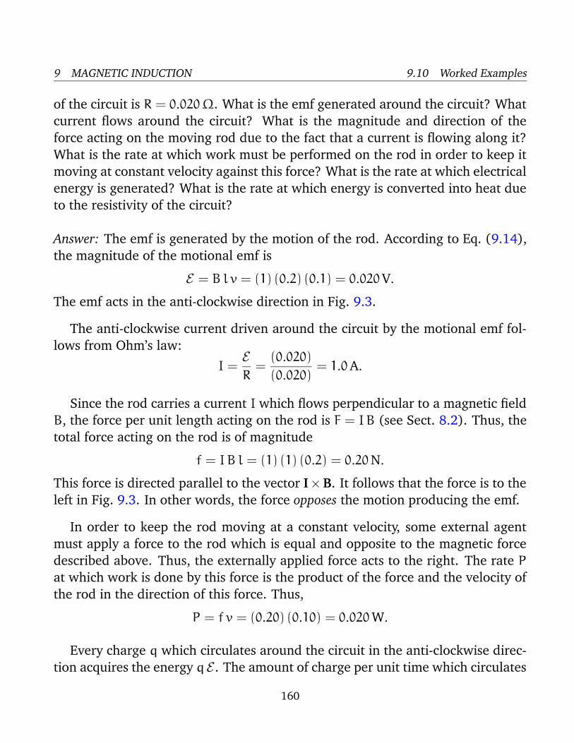
9 MAGNETIC INDUCTION 9.10 Worked Examples
of the circuit is R = 0.020 Ω. What is the emf generated around the circuit? What
current flows around the circuit? What is the magnitude and direction of the
force acting on the moving rod due to the fact that a current is flowing along it?
What is the rate at which work must be performed on the rod in order to keep it
moving at constant velocity against this force? What is the rate at which electrical
energy is generated? What is the rate at which energy is converted into heat due
to the resistivity of the circuit?
Answer: The emf is generated by the motion of the rod. According to Eq. (9.14),
the magnitude of the motional emf is
E = B l v = (1) (0.2) (0.1) = 0.020 V.
The emf acts in the anti-clockwise direction in Fig. 9.3.
The anti-clockwise current driven around the circuit by the motional emf fol-
lows from Ohm’s law:
I =ER
=(0.020)
(0.020)= 1.0 A.
Since the rod carries a current I which flows perpendicular to a magnetic field
B, the force per unit length acting on the rod is F = I B (see Sect. 8.2). Thus, the
total force acting on the rod is of magnitude
f = I B l = (1) (1) (0.2) = 0.20 N.
This force is directed parallel to the vector I×B. It follows that the force is to the
left in Fig. 9.3. In other words, the force opposes the motion producing the emf.
In order to keep the rod moving at a constant velocity, some external agent
must apply a force to the rod which is equal and opposite to the magnetic force
described above. Thus, the externally applied force acts to the right. The rate P
at which work is done by this force is the product of the force and the velocity of
the rod in the direction of this force. Thus,
P = f v = (0.20) (0.10) = 0.020 W.
Every charge q which circulates around the circuit in the anti-clockwise direc-
tion acquires the energy q E . The amount of charge per unit time which circulates
160

9 MAGNETIC INDUCTION 9.10 Worked Examples
around the circuit is, by definition, equal to the current I flowing around the cir-
cuit. Thus, the rate at which electric charges acquire energy in the circuit is
P = E I = (0.020) (1) = 0.020 W.
Now, the rate at which electric charges acquire energy in the circuit is equal to
the rate at which mechanical work is done on the rod by the external force, as
must be the case if energy is to be conserved. Thus, we can think of this circuit
as constituting a primitive generator which transforms mechanical into electrical
energy.
The rate at which electrical energy is converted into heat energy in the circuit
is
P = I2 R = (1) (1) (0.020) = 0.020 W.
Thus, all of the mechanical work done on the rod eventually ends up as heat
dissipated in the circuit.
Worked Example 4: AC generators
Question: A simple AC generator consists of an N = 10 turn coil of area A =
1200 cm2 which rotates at a constant frequency of f = 60 Hz in a B = 0.40 T mag-
netic field. What is the peak emf of the device?
Answer: The peak emf Emax is given by [see Eq. (9.22)]
Emax = 2π N B A f = (6.283) (10) (0.40) (0.12) (60) = 181 V.
Worked Example 5: AC motors
Question: An AC motor has an internal resistance of R = 4.0 Ω. When powered by
a 50 Hz AC supply of peak voltage V = 120 V it draws a peak current of I = 5.0 A.
What is the peak back-emf produced by the motor? What is the peak power de-
livered to the motor by the AC supply? What is the peak rate of energy loss as
161

9 MAGNETIC INDUCTION 9.10 Worked Examples
heat in the motor? What is the peak useful power produced by the motor? What
is the efficiency (i.e., the ratio of the peak useful power output to the peak power
delivered) of such a motor?
Answer: If V is the peak applied voltage, and E the peak back-emf, then the
peak applied voltage must equal the sum of the peak voltage drops across the
motor, or V = E + I R. It follows that
E = V − I R = (120) − (5.0) (4.0) = 100 V.
The peak power delivered by the AC supply is
P1 = V I = (120) (5.0) = 600 W.
Energy is lost as heat in the motor at the peak rate
P2 = I2 R = (5.0)2 (4.0) = 100 W.
The peak useful power produced by the motor is the difference between the peak
power supplied to the motor and the peak power dissipated as heat:
P = P1 − P2 = (600) − (100) = 500 W.
The peak useful power is also given by the product of the peak back-emf and the
peak current flowing through the motor [see Eq. (9.36)],
P = E I = (100) (5.0) = 500 W.
The efficiency η is the ratio of the peak useful power output of the motor to the
peak power supplied, or
η =P
P1
=500
600= 0.83 = 83 %.
162

10 INDUCTANCE
10 Inductance
10.1 Mutual Inductance
..
circuit 2I2
circuit 1
I1
Figure 10.1: Two inductively coupled circuits.
Consider two arbitrary conducting circuits, labelled 1 and 2. Suppose that I1
is the instantaneous current flowing around circuit 1. This current generates a
magnetic field B1 which links the second circuit, giving rise to a magnetic flux Φ2
through that circuit. If the current I1 doubles, then the magnetic field B1 doubles
in strength at all points in space, so the magnetic flux Φ2 through the second
circuit also doubles. This conclusion follows from the linearity of the laws of
magnetostatics, plus the definition of magnetic flux. Furthermore, it is obvious
that the flux through the second circuit is zero whenever the current flowing
around the first circuit is zero. It follows that the flux Φ2 through the second
circuit is directly proportional to the current I1 flowing around the first circuit.
Hence, we can write
Φ2 = M21 I1, (10.1)
where the constant of proportionality M21 is called the mutual inductance of cir-
cuit 2 with respect to circuit 1. Similarly, the flux Φ1 through the first circuit
due to the instantaneous current I2 flowing around the second circuit is directly
163

10 INDUCTANCE 10.1 Mutual Inductance
proportional to that current, so we can write
Φ1 = M12 I2, (10.2)
where M12 is the mutual inductance of circuit 1 with respect to circuit 2. It is
possible to demonstrate mathematically that M12 = M21. In other words, the flux
linking circuit 2 when a certain current flows around circuit 1 is exactly the same
as the flux linking circuit 1 when the same current flows around circuit 2. This
is true irrespective of the size, number of turns, relative position, and relative
orientation of the two circuits. Because of this, we can write
M12 = M21 = M, (10.3)
where M is termed the mutual inductance of the two circuits. Note that M is a
purely geometric quantity, depending only on the size, number of turns, relative
position, and relative orientation of the two circuits. The SI units of mutual
inductance are called Henries (H). One henry is equivalent to a volt-second per
ampere:
1 H ≡ 1 V s A−1. (10.4)
It turns out that a henry is a rather unwieldy unit. The mutual inductances of the
circuits typically encountered in laboratory experiments are measured in milli-
henries.
Suppose that the current flowing around circuit 1 changes by an amount dI1
in a time interval dt. It follows from Eqs. (10.1) and (10.3) that the flux linking
circuit 2 changes by an amount dΦ2 = M dI1 in the same time interval. According
to Faraday’s law, an emf
E2 = −dΦ2
dt(10.5)
is generated around the second circuit due to the changing magnetic flux linking
that circuit. Since, dΦ2 = M dI1, this emf can also be written
E2 = −MdI1
dt. (10.6)
Thus, the emf generated around the second circuit due to the current flowing
around the first circuit is directly proportional to the rate at which that current
164

10 INDUCTANCE 10.1 Mutual Inductance
changes. Likewise, if the current I2 flowing around the second circuit changes
by an amount dI2 in a time interval dt then the emf generated around the first
circuit is
E1 = −MdI2
dt. (10.7)
Note that there is no direct physical coupling between the two circuits. The
coupling is due entirely to the magnetic field generated by the currents flowing
around the circuits.
As a simple example, suppose that two insulated wires are wound on the same
cylindrical former, so as to form two solenoids sharing a common air-filled core.
Let l be the length of the core, A the cross-sectional area of the core, N1 the
number of times the first wire is wound around the core, and N2 the number of
times the second wire is wound around the core. If a current I1 flows around
the first wire then a uniform axial magnetic field of strength B1 = µ0 N1 I1/l is
generated in the core (see Sect. 8.8). The magnetic field in the region outside the
core is of negligible magnitude. The flux linking a single turn of the second wire
is B1 A. Thus, the flux linking all N2 turns of the second wire is Φ2 = N2 B1 A =
µ0 N1 N2 A I1/l. From Eq. (10.1), the mutual inductance of the second wire with
respect to the first is
M21 =Φ2
I1
=µ0 N1 N2 A
l. (10.8)
Now, the flux linking the second wire when a current I2 flows in the first wire is
Φ1 = N1 B2 A, where B2 = µ0 N2 I2/l is the associated magnetic field generated
in the core. It follows from Eq. (10.2) that the mutual inductance of the first wire
with respect to the second is
M12 =Φ1
I2
=µ0 N1 N2 A
l. (10.9)
Note that M21 = M12, in accordance with Eq. (10.3). Thus, the mutual induc-
tance of the two wires is given by
M =µ0 N1 N2 A
l. (10.10)
As described previously, M is a geometric quantity depending on the dimensions
of the core, and the manner in which the two wires are wound around the core,
but not on the actual currents flowing through the wires.
165

10 INDUCTANCE 10.2 Self Inductance
10.2 Self Inductance
We do not necessarily need two circuits in order to have inductive effects. Con-
sider a single conducting circuit around which a current I is flowing. This current
generates a magnetic field B which gives rise to a magnetic flux Φ linking the
circuit. We expect the flux Φ to be directly proportional to the current I, given
the linear nature of the laws of magnetostatics, and the definition of magnetic
flux. Thus, we can write
Φ = L I, (10.11)
where the constant of proportionality L is called the self inductance of the circuit.
Like mutual inductance, the self inductance of a circuit is measured in units of
henries, and is a purely geometric quantity, depending only on the shape of the
circuit and number of turns in the circuit.
If the current flowing around the circuit changes by an amount dI in a time
interval dt then the magnetic flux linking the circuit changes by an amount dΦ =
L dI in the same time interval. According to Faraday’s law, an emf
E = −dΦ
dt(10.12)
is generated around the circuit. Since dΦ = L dI, this emf can also be written
E = −LdI
dt. (10.13)
Thus, the emf generated around the circuit due to its own current is directly
proportional to the rate at which the current changes. Lenz’s law, and common
sense, demand that if the current is increasing then the emf should always act
to reduce the current, and vice versa. This is easily appreciated, since if the emf
acted to increase the current when the current was increasing then we would
clearly get an unphysical positive feedback effect in which the current continued
to increase without limit. It follows, from Eq. (10.13), that the self inductance
L of a circuit is necessarily a positive number. This is not the case for mutual
inductances, which can be either positive or negative.
Consider a solenoid of length l and cross-sectional area A. Suppose that the
solenoid has N turns. When a current I flows in the solenoid, a uniform axial
166

10 INDUCTANCE 10.3 Energy Stored in an Inductor
field of magnitude
B =µ0 N I
l(10.14)
is generated in the core of the solenoid. The field-strength outside the core is
negligible. The magnetic flux linking a single turn of the solenoid is Φ = B A.
Thus, the magnetic flux linking all N turns of the solenoid is
Φ = N B A =µ0 N2 A I
l. (10.15)
According to Eq. (10.11), the self inductance of the solenoid is given by L = Φ/I,
which reduces to
L =µ0 N2 A
l. (10.16)
Note that L is positive. Furthermore, L is a geometric quantity depending only on
the dimensions of the solenoid, and the number of turns in the solenoid.
Engineers like to reduce all pieces of electrical apparatus, no matter how com-
plicated, to an equivalent circuit consisting of a network of just four different types
of component. These four basic components are emfs, resistors, capacitors, and in-
ductors. An inductor is simply a pure self inductance, and is usually represented a
little solenoid in circuit diagrams. In practice, inductors generally consist of short
air-cored solenoids wound from enameled copper wire.
10.3 Energy Stored in an Inductor
Suppose that an inductor of inductance L is connected to a variable DC voltage
supply. The supply is adjusted so as to increase the current i flowing through the
inductor from zero to some final value I. As the current through the inductor is
ramped up, an emf E = −L di/dt is generated, which acts to oppose the increase
in the current. Clearly, work must be done against this emf by the voltage source
in order to establish the current in the inductor. The work done by the voltage
source during a time interval dt is
dW = P dt = −E i dt = i Ldi
dtdt = L i di. (10.17)
167

10 INDUCTANCE 10.3 Energy Stored in an Inductor
Here, P = −E i is the instantaneous rate at which the voltage source performs
work. To find the total work W done in establishing the final current I in the
inductor, we must integrate the above expression. Thus,
W = L
∫ I
0
i di, (10.18)
giving
W =1
2L I2. (10.19)
This energy is actually stored in the magnetic field generated by the current flow-
ing through the inductor. In a pure inductor, the energy is stored without loss,
and is returned to the rest of the circuit when the current through the inductor is
ramped down, and its associated magnetic field collapses.
Consider a simple solenoid. Equations (10.14), (10.16), and (10.19) can be
combined to give
W =1
2L I2 =
µ0 N2 A
2 l
(
B l
µ0 N
)2
, (10.20)
which reduces to
W =B2
2 µ0
l A. (10.21)
This represents the energy stored in the magnetic field of the solenoid. However,
the volume of the field-filled core of the solenoid is l A, so the magnetic energy
density (i.e., the energy per unit volume) inside the solenoid is w = W/(l A), or
w =B2
2 µ0
. (10.22)
It turns out that this result is quite general. Thus, we can calculate the energy
content of any magnetic field by dividing space into little cubes (in each of which
the magnetic field is approximately uniform), applying the above formula to find
the energy content of each cube, and summing the energies thus obtained to find
the total energy.
When electric and magnetic fields exist together in space, Eqs. (6.23) and
(10.22) can be combined to give an expression for the total energy stored in the
168

10 INDUCTANCE 10.4 The RL Circuit
combined fields per unit volume:
w =ε0 E2
2+
B2
2 µ0
. (10.23)
10.4 The RL Circuit
Consider a circuit in which a battery of emf V is connected in series with an
inductor of inductance L and a resistor of resistance R. For obvious reasons,
this type of circuit is usually called an RL circuit. The resistance R includes the
resistance of the wire loops of the inductor, in addition to any other resistances
in the circuit.
In steady-state, the current I flowing around the the circuit has the magnitude
I =V
R(10.24)
specified by Ohm’s law. Note that, in a steady-state, or DC, circuit, zero back-emf
is generated by the inductor, according to Eq. (10.13), so the inductor effectively
disappears from the circuit. In fact, inductors have no effect whatsoever in DC
circuits. They just act like pieces of conducting wire.
.
.
RL
Vswitch
i
Figure 10.2: An RL circuit with a switch.
Let us now slightly modify our RL circuit by introducing a switch. The new
circuit is shown in Fig. 10.2. Suppose that the switch is initially open, but is
169

10 INDUCTANCE 10.4 The RL Circuit
suddenly closed at t = 0. Obviously, we expect the instantaneous current i which
flows around the circuit, once the switch is thrown, to eventually settle down
to the steady-state value I = V/R. But, how long does this process take? Note
that as the current flowing around the circuit is building up to its final value, a
non-zero back-emf is generated in the inductor, according to Eq. (10.13). Thus,
although the inductor does not affect the final steady-state value of the current
flowing around the circuit, it certainly does affect how long after the switch is
closed it takes for this final current to be established.
If the instantaneous current i flowing around the circuit changes by an amount
di in a short time interval dt, then the emf generated in the inductor is given by
[see Eq. (10.13)]
E = −Ldi
dt. (10.25)
Applying Ohm’s law around the circuit, we obtain
V + E = i R, (10.26)
which yields
− Ldi
dt= i R − V. (10.27)
Let
i ′ = i − I, (10.28)
where I = V/R is the steady-state current. Equation (10.27) can be rewritten
di ′
dt= −i ′
R
L, (10.29)
since di ′ = di (because I is non-time-varying). At t = 0, just after the switch is
closed, we expect the current i flowing around the circuit to be zero. It follows
from Eq. (10.28) that
i ′(t = 0) = −I. (10.30)
Integration of Eq. (10.29), subject to the initial condition (10.30), yields
i ′(t) = −I e−R t/L. (10.31)
170

10 INDUCTANCE 10.4 The RL Circuit
00
I
i
->
t ->
Figure 10.3: Sketch of the current rise phase in an RL circuit switched on at t = 0.
Thus, it follows from Eq. (10.28) that
i(t) = I (1 − e−R t/L). (10.32)
The above expression specifies the current i flowing around the circuit a time
interval t after the switch is closed (at time t = 0). The variation of the current
with time is sketched in Fig. 10.3. It can be seen that when the switch is closed the
current i flowing in the circuit does not suddenly jump up to its final value, I =
V/R. Instead, the current increases smoothly from zero, and gradually asymptotes
to its final value. The current has risen to approximately 63% of its final value a
time
τ =L
R(10.33)
after the switch is closed (since e−1 ' 0.37). By the time t = 5 τ, the current
has risen to more than 99% of its final value (since e−5 < 0.01). Thus, τ = L/R
is a good measure of how long after the switch is closed it takes for the current
flowing in the circuit to attain its steady-state value. The quantity τ is termed the
time-constant, or, somewhat unimaginatively, the L over R time, of the circuit.
Suppose that the current flowing in the circuit discussed above has settled
down to its steady-state value I = V/R. Consider what would happen if we were
to suddenly (at t = 0, say) switch the battery out of the circuit, and replace it by
a conducting wire. Obviously, we would expect the current to eventually decay
away to zero, since there is no longer a steady emf in the circuit to maintain a
steady current. But, how long does this process take?
171

10 INDUCTANCE 10.4 The RL Circuit
Applying Ohm’s law around the circuit, in the absence of the battery, we obtain
E = i R, (10.34)
where E = −L di/dt is the back-emf generated by the inductor, and i is the
instantaneous current flowing around the circuit. The above equation reduces to
di
dt= −i
R
L. (10.35)
At t = 0, immediately after the battery is switched out of the circuit, we expect
the current i flowing around the circuit to equal its steady-state value I, so that
i(t = 0) = I. (10.36)
Integration of Eq. (10.35), subject to the boundary condition (10.36), yields
i(t) = I e−R t/L. (10.37)
According to the above formula, once the battery is switched out of the circuit,
the current decays smoothly to zero. After one L/R time (i.e., t = L/R), the
current has decayed to 37% of its initial value. After five L/R times, the current
has decayed to less than 1% of its initial value.
We can now appreciate the significance of self inductance. The back-emf gen-
erated in an inductor, as the current flowing through it tries to change, effectively
prevents the current from rising (or falling) much faster than the L/R time of the
circuit. This effect is sometimes advantageous, but is often a great nuisance. All
circuits possess some self inductance, as well as some resistance, so all have a
finite L/R time. This means that when we power up a DC circuit, the current
does not jump up instantaneously to its steady-state value. Instead, the rise is
spread out over the L/R time of the circuit. This is a good thing. If the current
were to rise instantaneously then extremely large inductive electric fields would
be generated by the sudden jump in the magnetic field, leading, inevitably, to
breakdown and electric arcing. So, if there were no such thing as self inductance
then every time we switched a DC electric circuit on or off there would be a big
blue flash due to arcing between conductors. Self inductance can also be a bad
thing. Suppose that we possess a fancy power supply, and wish to use it to send
172
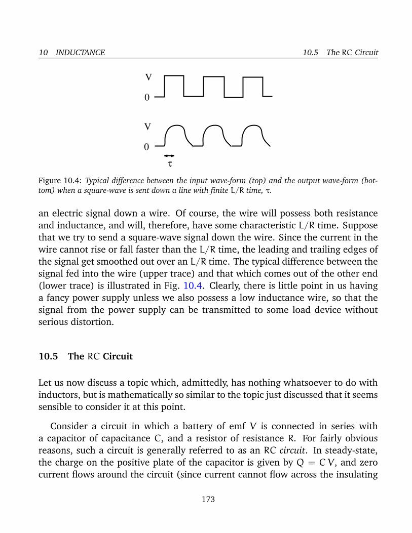
10 INDUCTANCE 10.5 The RC Circuit
0
V
0
V
τ
Figure 10.4: Typical difference between the input wave-form (top) and the output wave-form (bot-
tom) when a square-wave is sent down a line with finite L/R time, τ.
an electric signal down a wire. Of course, the wire will possess both resistance
and inductance, and will, therefore, have some characteristic L/R time. Suppose
that we try to send a square-wave signal down the wire. Since the current in the
wire cannot rise or fall faster than the L/R time, the leading and trailing edges of
the signal get smoothed out over an L/R time. The typical difference between the
signal fed into the wire (upper trace) and that which comes out of the other end
(lower trace) is illustrated in Fig. 10.4. Clearly, there is little point in us having
a fancy power supply unless we also possess a low inductance wire, so that the
signal from the power supply can be transmitted to some load device without
serious distortion.
10.5 The RC Circuit
Let us now discuss a topic which, admittedly, has nothing whatsoever to do with
inductors, but is mathematically so similar to the topic just discussed that it seems
sensible to consider it at this point.
Consider a circuit in which a battery of emf V is connected in series with
a capacitor of capacitance C, and a resistor of resistance R. For fairly obvious
reasons, such a circuit is generally referred to as an RC circuit. In steady-state,
the charge on the positive plate of the capacitor is given by Q = C V , and zero
current flows around the circuit (since current cannot flow across the insulating
173

10 INDUCTANCE 10.5 The RC Circuit
.
R
Vswitch
i
C
Figure 10.5: An RC circuit with a switch.
gap between the capacitor plates).
Let us now introduce a switch into the circuit, as shown in Fig. 10.5. Suppose
that the switch is initially open, but is suddenly closed at t = 0. It is assumed
that the capacitor plates are uncharged when the switch is thrown. We expect a
transient current i to flow around the circuit until the charge q on the positive
plate of the capacitor attains its final steady-state value Q = C V . But, how long
does this process take?
The potential difference v between the positive and negative plates of the ca-
pacitor is given by
v = V − i R. (10.38)
In other words, the potential difference between the plates is the emf of the
battery minus the potential drop across the resistor. The charge q on the positive
plate of the capacitor is written
q = C v = Q − i R C, (10.39)
where Q = C V is the final charge. Now, if i is the instantaneous current flowing
around the circuit, then in a short time interval dt the charge on the positive plate
of the capacitor increases by a small amount dq = i dt (since all of the charge
which flows around the circuit must accumulate on the plates of the capacitor).
It follows that
i =dq
dt. (10.40)
174

10 INDUCTANCE 10.5 The RC Circuit
Thus, the instantaneous current flowing around the circuit is numerically equal
to the rate at which the charge accumulated on the positive plate of the capacitor
increases with time. Equations (10.39) and (10.40) can be combined together to
givedq ′
dt= −
q ′
R C, (10.41)
where
q ′ = q − Q. (10.42)
At t = 0, just after the switch is closed, the charge on the positive plate of the
capacitor is zero, so
q ′(t = 0) = −Q. (10.43)
Integration of Eq. (10.41), subject to the boundary condition (10.43), yields
q ′(t) = −Q e−t/RC. (10.44)
It follows from Eq. (10.42) that
q(t) = Q (1 − e−t/RC). (10.45)
The above expression specifies the charge q on the positive plate of the capacitor
a time interval t after the switch is closed (at time t = 0). The variation of the
charge with time is sketched in Fig. 10.6. It can be seen that when the switch is
closed the charge q on the positive plate of the capacitor does not suddenly jump
up to its final value, Q = C V . Instead, the charge increases smoothly from zero,
and gradually asymptotes to its final value. The charge has risen to approximately
63% of its final value a time
τ = R C (10.46)
after the switch is closed. By the time t = 5 τ, the charge has risen to more than
99% of its final value. Thus, τ = R C is a good measure of how long after the
switch is closed it takes for the capacitor to fully charge up. The quantity τ is
termed the time-constant, or the RC time, of the circuit.
According to Eqs. (10.40) and (10.41),
i =dq
dt=
dq ′
dt= −
q ′
R C. (10.47)
175

10 INDUCTANCE 10.5 The RC Circuit
00
->
t ->
q
Q
Figure 10.6: Sketch of the charging phase in an RC circuit switched on at t = 0.
It follows from Eq. (10.44) that
i(t) = I e−t/RC, (10.48)
where I = V/R. The above expression specifies the current i flowing around
the circuit a time interval t after the switch is closed (at time t = 0). It can be
seen that, immediately after the switch is thrown, the current I = V/R which
flows in the circuit is that which would flow if the capacitor were replaced by
a conducting wire. However, this current is only transient, and rapidly decays
away to a negligible value. After one RC time, the current has decayed to 37% of
its initial value. After five RC times, the current has decayed to less than 1% of
its initial value. It is interesting to note that for a short instant of time, just after
the switch is closed, the current in the circuit acts as if there is no insulating gap
between the capacitor plates. It essentially takes an RC time for the information
about the break in the circuit to propagate around the circuit, and cause the
current to stop flowing.
Suppose that we take a capacitor of capacitance C, which is charged to a
voltage V , and discharge it by connecting a resistor of resistance R across its
terminals at t = 0. How long does it take for the capacitor to discharge? By
analogy with the previous analysis, the charge q on the positive plate of the
capacitor at time t is given by
q(t) = Q e−t/RC, (10.49)
where Q = C V is the initial charge on the positive plate. It can be seen that it
takes a few RC times for the capacitor to fully discharge. The current i which
176

10 INDUCTANCE 10.6 Transformers
flows through the resistor is
i(t) = I e−t/RC, (10.50)
where I = V/R is the initial current. It can be seen that the capacitor initially acts
like a battery of emf V (since it drives the current I = V/R across the resistor),
but that, as it discharges, its effective emf decays to a negligible value on a few
RC times.
10.6 Transformers
A transformer is a device for stepping-up, or stepping-down, the voltage of an
alternating electric signal. Without efficient transformers, the transmission and
distribution of AC electric power over long distances would be impossible. Fig-
ure 10.7 shows the circuit diagram of a typical transformer. There are two cir-
cuits. Namely, the primary circuit, and the secondary circuit. There is no direct
electrical connection between the two circuits, but each circuit contains a coil
which links it inductively to the other circuit. In real transformers, the two coils
are wound onto the same iron core. The purpose of the iron core is to channel the
magnetic flux generated by the current flowing around the primary coil, so that
as much of it as possible also links the secondary coil. The common magnetic flux
linking the two coils is conventionally denoted in circuit diagrams by a number
of parallel straight lines drawn between the coils.
Let us consider a particularly simple transformer in which the primary and
secondary coils are solenoids sharing the same air-filled core. Suppose that l
is the length of the core, and A is its cross-sectional area. Let N1 be the total
number of turns in the primary coil, and let N2 be the total number of turns in
the secondary coil. Suppose that an alternating voltage
v1 = V1 cos(ω t) (10.51)
is fed into the primary circuit from some external AC power source. Here, V1 is
the peak voltage in the primary circuit, and ω is the alternation frequency (in
radians per second). The current driven around the primary circuit is written
i1 = I1 sin(ω t), (10.52)
177

10 INDUCTANCE 10.6 Transformers
.
~
primary circuit secondary circuit
1
2
2
1
v
i i
v. .
core
Figure 10.7: Circuit diagram of a transformer.
where I1 is the peak current. This current generates a changing magnetic flux, in
the core of the solenoid, which links the secondary coil, and, thereby, inductively
generates the alternating emf
v2 = V2 cos(ω t) (10.53)
in the secondary circuit, where V2 is the peak voltage. Suppose that this emf
drives an alternating current
i2 = I2 sin(ω t) (10.54)
around the secondary circuit, where I2 is the peak current.
The circuit equation for the primary circuit is written
v1 − L1
di1
dt− M
di2
dt= 0, (10.55)
assuming that there is negligible resistance in this circuit. The first term in the
above equation is the externally generated emf. The second term is the back-emf
due to the self inductance L1 of the primary coil. The final term is the emf due to
the mutual inductance M of the primary and secondary coils. In the absence of
any significant resistance in the primary circuit, these three emfs must add up to
zero. Equations (10.51), (10.52), (10.54), and (10.55) can be combined to give
V1 = ω (L1 I1 + M I2), (10.56)
178

10 INDUCTANCE 10.6 Transformers
sinced sin(ω t)
dt= ω cos(ω t). (10.57)
The alternating emf generated in the secondary circuit consists of the emf
generated by the self inductance L2 of the secondary coil, plus the emf generated
by the mutual inductance of the primary and secondary coils. Thus,
v2 = L2
di2
dt+ M
di1
dt. (10.58)
Equations (10.52), (10.53), (10.54), (10.57), and (10.58) yield
V2 = ω (L2 I2 + M I1). (10.59)
Now, the instantaneous power output of the external AC power source which
drives the primary circuit is
P1 = i1 v1. (10.60)
Likewise, the instantaneous electrical energy per unit time transfered inductively
from the primary to the secondary circuit is
P2 = i2 v2. (10.61)
If resistive losses in the primary and secondary circuits are negligible, as is as-
sumed to be the case, then, by energy conservation, these two powers must equal
one another at all times. Thus,
i1 v1 = i2 v2, (10.62)
which easily reduces to
I1 V1 = I2 V2. (10.63)
Equations (10.56), (10.59), and (10.63) yield
I1 V1 = ω (L1 I 21 + M I1 I2) = ω (L2 I 2
2 + M I1 I2) = I2 V2, (10.64)
which gives
ω L1 I 21 = ω L2 I 2
2 , (10.65)
179

10 INDUCTANCE 10.6 Transformers
and, hence,I1
I2
=
√
√
√
√
L2
L1
. (10.66)
Equations (10.63) and (10.66) can be combined to give
V1
V2
=
√
√
√
√
L1
L2
. (10.67)
Note that, although the mutual inductance of the two coils is entirely responsible
for the transfer of energy between the primary and secondary circuits, it is the
self inductances of the two coils which determine the ratio of the peak voltages
and peak currents in these circuits.
Now, from Sect. 10.2, the self inductances of the primary and secondary coils
are given by L1 = µ0 N 21 A/l and L2 = µ0 N 2
2 A/l, respectively. It follows that
L1
L2
=
(
N1
N2
)2
, (10.68)
and, hence, thatV1
V2
=I2
I1
=N1
N2
. (10.69)
In other words, the ratio of the peak voltages and peak currents in the primary
and secondary circuits is determined by the ratio of the number of turns in the
primary and secondary coils. This latter ratio is usually called the turns-ratio of
the transformer. If the secondary coil contains more turns than the primary coil
then the peak voltage in the secondary circuit exceeds that in the primary circuit.
This type of transformer is called a step-up transformer, because it steps up the
voltage of an AC signal. Note that in a step-up transformer the peak current in
the secondary circuit is less than the peak current in the primary circuit (as must
be the case if energy is to be conserved). Thus, a step-up transformer actually
steps down the current. Likewise, if the secondary coil contains less turns than
the primary coil then the peak voltage in the secondary circuit is less than that
in the primary circuit. This type of transformer is called a step-down transformer.
Note that a step-down transformer actually steps up the current (i.e., the peak
current in the secondary circuit exceeds that in the primary circuit).
180
10 INDUCTANCE 10.6 Transformers
AC electricity is generated in power stations at a fairly low peak voltage (i.e.,
something like 440 V), and is consumed by the domestic user at a peak voltage of
110 V (in the U.S.). However, AC electricity is transmitted from the power station
to the location where it is consumed at a very high peak voltage (typically 50 kV).
In fact, as soon as an AC signal comes out of a generator in a power station it is
fed into a step-up transformer which boosts its peak voltage from a few hundred
volts to many tens of kilovolts. The output from the step-up transformer is fed
into a high tension transmission line, which typically transports the electricity
over many tens of kilometers, and, once the electricity has reached its point of
consumption, it is fed through a series of step-down transformers until, by the
time it emerges from a domestic power socket, its peak voltage is only 110 V.
But, if AC electricity is both generated and consumed at comparatively low peak
voltages, why go to the trouble of stepping up the peak voltage to a very high
value at the power station, and then stepping down the voltage again once the
electricity has reached its point of consumption? Why not generate, transmit,
and distribute the electricity at a peak voltage of 110 V? Well, consider an electric
power line which transmits a peak electric power P between a power station and
a city. We can think of P, which depends on the number of consumers in the city,
and the nature of the electrical devices which they operate, as essentially a fixed
number. Suppose that V and I are the peak voltage and peak current of the AC
signal transmitted along the line, respectively. We can think of these numbers as
being variable, since we can change them using a transformer. However, since
P = I V , the product of the peak voltage and the peak current must remain
constant. Suppose that the resistance of the line is R. The peak rate at which
electrical energy is lost due to ohmic heating in the line is PR = I2 R, which can
be written
PR =P2 R
V2. (10.70)
Thus, if the power P transmitted down the line is a fixed quantity, as is the resis-
tance R of the line, then the power lost in the line due to ohmic heating varies like
the inverse square of the peak voltage in the line. It turns out that even at very
high voltages, such as 50 kV, the ohmic power losses in transmission lines which
run over tens of kilometers can amount to up to 20% of the transmitted power. It
can readily be appreciated that if an attempt were made to transmit AC electric
181

10 INDUCTANCE 10.7 Impedance Matching
power at a peak voltage of 110 V then the ohmic losses would be so severe that
virtually none of the power would reach its destination. Thus, it is only possible
to generate electric power at a central location, transmit it over large distances,
and then distribute it at its point of consumption, if the transmission is performed
at a very high peak voltages (the higher, the better). Transformers play a vital
role in this process because they allow us to step-up and step-down the voltage
of an AC electric signal very efficiently (a well-designed transformer typically has
a power loss which is only a few percent of the total power flowing through it).
Of course, transformers do not work for DC electricity, because the magnetic
flux generated by the primary coil does not vary in time, and, therefore, does
not induce an emf in the secondary coil. In fact, there is no efficient method
of stepping-up or stepping-down the voltage of a DC electric signal. Thus, it is
impossible to efficiently transmit DC electric power over larger distances. This is
the main reason why commercially generated electricity is AC, rather than DC.
10.7 Impedance Matching
The principle use of transformers is in the transmission and distribution of com-
mercially generated electricity. However, a second, very important use of trans-
formers is as impedance matching devices. Recall, from Sect. 7.9, that for max-
imum power delivery from a source to a load, the load must have the same re-
sistance as the internal resistance of the source. This can be accomplished by
using a transformer to match the two resistances. Suppose that the power source
is connected to the primary circuit, and the load to the secondary. If the resis-
tance of the load is R, then R = V2/I2. However, from the transformer equation,
(10.69), we have
V1 =N1
N2
V2, (10.71)
and
I1 =N2
N1
I2. (10.72)
182

10 INDUCTANCE 10.8 Worked Examples
Now the effective resistance R ′ of the load in the primary circuit is given by
R ′ =V1
I1
=
(
N1
N2
)2 V2
I2
, (10.73)
which easily reduces to
R ′ =
(
N1
N2
)2
R. (10.74)
Thus, by choosing the appropriate turns ratio, the effective load resistance R ′ can
be made equal to the internal resistance of the source, no matter what value the
actual load resistance R takes. This process is called impedance matching.
10.8 Worked Examples
Example 10.1: Mutual induction
Question: Suppose that two insulated wires are wound onto a common cylindri-
cal former of length l = 0.1 m and cross-sectional area A = 0.05 m2. The number
of turns in the first wire is N1 = 100, and the number of turns in the second wire
is N2 = 300. What is the mutual inductance of the two wires? If the current I1
flowing in the first wire increases uniformly from 0 to 10 A in 0.1 s, what emf is
generated in the second wire? Does this emf act to drive a current in the second
wire which circulates in the same sense as the current in the first wire, or the
opposite sense?
Answer: From Eq. (10.10), the mutual inductance of the two wires is
M =µ0 N1 N2 A
l=
(1.26 × 10⁻⁶) (100) (300) (0.05)
0.1= 0.0188 H.
From Eq. (10.6), the emf generated around the second loop by the changing
current in the first loop is
E2 = −MdI1
dt= −(0.0188)
(10 − 0)
(0.1)= −1.88 V.
183

10 INDUCTANCE 10.8 Worked Examples
The minus sign indicates that this emf acts so as to drive a current in the second
wire which circulates in the opposite sense to the current flowing in the first wire,
in accordance with Lenz’s law. If the current in the first wire were decreased,
instead of increased, then the emf in the second wire would act to drive a current
which circulates in the same sense as the former current.
Example 10.2: Energy density of electric and magnetic fields
Question: In a certain region of space, the magnetic field has a value of 1.0 ×10⁻² T, and the electric field has a value of 2.0× 10⁶ V m−1. What is the combined
energy density of the electric and magnetic fields?
Answer: For the electric field, the energy density is
wE =1
2ε0 E2 = (0.5) (8.85 × 10⁻¹²) (2.0 × 10⁶)2 = 18 J m−3.
For the magnetic field, the energy density is
wB =1
2
B2
µ0
=(0.5) (1.0 × 10⁻²)2
(4π × 10−7)= 40 J m−3.
The net energy density is the sum of the energy density due to the electric field
and the energy density due to the magnetic field:
w = wE + wB = (18 + 40) = 58 J m−3.
Example 10.3: The RL circuit
Question: A coil has a resistance of R = 5.0 Ω and an inductance of L = 100 mH.
At a particular instant in time after a battery is connected across the coil, the
current is i = 2.0 A, and is increasing at a rate of di/dt = 20 A s−1. What is the
voltage V of the battery? What is the time-constant of the circuit? What is the
final value of the current?
184

10 INDUCTANCE 10.8 Worked Examples
Answer: Application of Ohm’s law around the circuit gives [see Eq. (10.27)]
V = i R + Ldi
dt= (2.0) (5.0) + (0.1) (20) = 12 V.
The time-constant of the circuit is simply
τ =L
R=
(0.1)
(5.0)= 0.020 s.
The final steady-state current I is given by Ohm’s law, with the inductor acting
like a conducting wire, so
I =V
R=
(12)
(5)= 2.4 A.
Example 10.4: The RC circuit
Question: A capacitor of capacitance C = 15 µF is charged up to a voltage of
V = 800 V, and then discharged by connecting a resistor of resistance R = 8 MΩ
across its terminals. How long does it take for the charge on the positive plate of
the capacitor to be reduced to 10% of its original value?
Answer: Suppose that the resistor is first connected across the capacitor at t = 0.
The charge q on the positive plate of the capacitor is given by
q(t) = Q e−t/RC,
which can be rearranged to give
Q
q= e t/RC.
Taking the natural logarithm of both sides, we obtain
ln
(
Q
q
)
=t
R C.
185

10 INDUCTANCE 10.8 Worked Examples
Hence,
t = τ ln
(
Q
q
)
,
where
τ = R C = (8) (15) = 120 s
is the RC time. Since q/Q = 0.1, in this case, it follows that
t = (120) (ln 10) = 276.3 s.
Example 10.5: The step-up transformer
Question: An electric power plant produces P = 1 GW of AC electric power at a
peak voltage of V1 = 500 V. If it is desired to transmit this power at a peak volt-
age of V2 = 50 kV, what is the appropriate turns-ratio of the step-up transformer?
What peak current I1 would be sent over the transmission line if the peak voltage
were V1 = 500 V? What peak current I2 would be sent over the transmission line
if the peak voltage were V2 = 50 kV? What is the ratio of the ohmic powers losses
in the line in the two cases?
Answer: The appropriate turns-ratio is
N2
N1
=(5 × 10⁴)
(500)= 100.
Since the peak power is given by P = I1 V1, it follows that
I1 =P
V1
=(1 × 10⁹)
(500)= 2 MA.
Since the peak power remains unchanged after the signal passes through the
transformer (assuming that there are no power losses in the transformer), we
have
I2 =P
V2
=(1 × 10⁹)
(5 × 10⁴)= 20 kA.
186
10 INDUCTANCE 10.8 Worked Examples
The ratio of the power lost to ohmic heating in the two cases is
P1
P2
=I 21 R
I 22 R
=
2 × 10⁶
2 × 10⁴
2
= 10000,
where R is the resistance of the transmission line. Note that the ohmic power loss
is much greater at low peak voltage than at high peak voltage.
Example 10.6: Impedance matching
Question: An audio amplifier with an internal resistance of 2.0 kΩ is used to drive
a loudspeaker with a resistance of R = 5.0 Ω. A transformer is used to connect
the amplifier to the loudspeaker. What is the appropriate turns-ratio of the trans-
former for optimal power transfer between the amplifier and the loudspeaker?
Answer: We require the transformer to convert the actual resistance R of the
loudspeaker into an effective resistance R ′ which matches the internal resistance
2.0 kΩ of the amplifier. Thus, from Eq. (10.74),
N1
N2
=
√
√
√
√
R ′
R=
√
√
√
√
2 × 10³
5= 20.
187

11 ELECTROMAGNETIC WAVES
11 Electromagnetic Waves
11.1 Maxwell’s Equations
In the latter half of the nineteenth century, the Scottish physicist James Clerk
Maxwell demonstrated that all previously established experimental facts regard-
ing electric and magnetic fields could be summed up in just four equations. Nowa-
days, these equations are generally known as Maxwell’s equations.
The first equation is simply Gauss’ law (see Sect. 4). This equation describes
how electric charges generate electric fields. Gauss’ law states that:
The electric flux through any closed surface is equal to the total charge
enclosed by the surface, divided by ε0.
This can be written mathematically as∮
S
E · dS =Q
ε0
, (11.1)
where S is a closed surface enclosing the charge Q. The above expression can
also be written ∮
S
E · dS =1
ε0
∫
V
ρ dV, (11.2)
where V is a volume bounded by the surface S, and ρ is the charge density: i.e.,
the electric charge per unit volume.
The second equation is the magnetic equivalent of Gauss’ law (see Sect. 8.10).
This equation describes how the non-existence of magnetic monopoles causes
magnetic field-lines to form closed loops. Gauss’ law for magnetic fields states
that:
The magnetic flux through any closed surface is equal to zero.
This can be written mathematically as∫
S
B · dS = 0, (11.3)
188

11 ELECTROMAGNETIC WAVES 11.1 Maxwell’s Equations
where S is a closed surface.
The third equation is Faraday’s law (see Sect. 9.3). This equation describes
how changing magnetic fields generate electric fields. Faraday’s law states that:
The line integral of the electric field around any closed loop is equal to minus
the time rate of change of the magnetic flux through the loop.
This can be written mathematically as∮
C
E · dS = −d
dt
∫
S ′
B · dS ′, (11.4)
where S ′ is a surface attached to the loop C.
The fourth, and final, equation is Ampere’s circuital law (see Sect. 8.7). This
equation describes how electric currents generates magnetic fields. Ampere’s
circuital law states that:
The line integral of the magnetic field around any closed loop is equal to µ0
times the algebraic sum of the currents which pass through the loop.
This can be written mathematically as∮
C
B · dr = µ0 I, (11.5)
where I is the net current flowing through loop C. This equation can also be
written ∮
C
B · dr = µ0
∫
S ′
j · dS ′, (11.6)
where S ′ is a surface attached to the loop C, and j is the current density: i.e., the
electrical current per unit area.
When Maxwell first wrote Eqs. (11.2), (11.3), (11.4), and (11.6) he was basi-
cally trying to summarize everything which was known at the time about electric
and magnetic fields in mathematical form. However, the more Maxwell looked at
189

11 ELECTROMAGNETIC WAVES 11.1 Maxwell’s Equations
his equations, the more convinced he became that they were incomplete. Even-
tually, he proposed adding a new term, called the displacement current, to the
right-hand side of his fourth equation. In fact, Maxwell was able to show that
(11.2), (11.3), (11.4), and (11.6) are mathematically inconsistent unless the dis-
placement current term is added to Eq. (11.6). Unfortunately, Maxwell’s demon-
stration of this fact requires some advanced mathematical techniques which lie
well beyond the scope of this course. In the following, we shall give a highly
simplified version of his derivation of the missing term.
.
R
Vswitch
i E
C
Figure 11.1: Circuit containing a charging capacitor.
Consider a circuit consisting of a parallel plate capacitor of capacitance C in
series with a resistance R and an steady emf V , as shown in Fig. 11.1. Let A be
the area of the capacitor plates, and let d be their separation. Suppose that the
switch is closed at t = 0. The current i flowing around the circuit starts from
an initial value of I = V/R, and gradually decays to zero on the RC time of the
circuit (see Sect. 10.5). Simultaneously, the charge q on the positive plates of the
capacitor starts from zero, and gradually increases to a final value of Q = C V .
As the charge q varies, so does the potential difference v between the capacitor
plates, since v = q/C.
The electric field in the region between the plates is approximately uniform,
directed perpendicular to the plates (running from the positively charged plate
to the negatively charged plate), and is of magnitude E = v/d. It follows that
q = C v = C d E. (11.7)
In a time interval dt, the charge on the positive plate of the capacitor increases by
190

11 ELECTROMAGNETIC WAVES 11.1 Maxwell’s Equations
an amount dq = C d dE, where dE is the corresponding increase in the electric
field-strength between the plates. Note that both C and d are time-independent
quantities. It follows thatdq
dt= C d
dE
dt. (11.8)
Now, dq/dt is numerically equal to the instantaneous current i flowing around
the circuit (since all of the charge which flows around the circuit must accumulate
on the plates of the capacitor). Also, C = ε0 A/d for a parallel plate capacitor.
Hence, we can write
i =dq
dt= C d
dE
dt= ε0 A
dE
dt. (11.9)
Since the electric field E is normal to the area A, we can also write
i = ε0 AdE⊥dt
. (11.10)
Equation (11.10) relates the instantaneous current flowing around the circuit
to the time rate of change of the electric field between the capacitor plates. Ac-
cording to Eq. (11.6), the current flowing around the circuit generates a magnetic
field. This field circulates around the current carrying wires connecting the vari-
ous components of the circuit. However, since there is no actual current flowing
between the plates of the capacitor, no magnetic field is generated in this region,
according to Eq. (11.6). Maxwell demonstrated that for reasons of mathematical
self-consistency there must, in fact, be a magnetic field generated in the region
between the plates of the capacitor. Furthermore, this magnetic field must be the
same as that which would be generated if the current i (i.e., the same current as
that which flows around the rest of the circuit) flowed between the plates. Of
course, there is no actual current flowing between the plates. However, there is a
changing electric field. Maxwell argued that a changing electric field constitutes
an effective current (i.e., it generates a magnetic field in just the same manner
as an actual current). For historical reasons (which do not particularly interest
us at the moment), Maxwell called this type of current a displacement current.
Since the displacement current ID flowing between the plates of the capacitor
must equal the current i flowing around the rest of the circuit, it follows from
191

11 ELECTROMAGNETIC WAVES 11.1 Maxwell’s Equations
Eq. (11.10) that
ID = ε0 AdE⊥dt
. (11.11)
Equation (11.11) was derived for the special case of the changing electric field
generated in the region between the plates of a charging parallel plate capaci-
tor. Nevertheless, this equation turns out to be completely general. Note that
A E⊥ is equal to the electric flux ΦE between the plates of the capacitor. Thus,
the most general expression for the displacement current passing through some
closed loop is
ID = ε0
dΦE
dt, (11.12)
where ΦE is the electric flux through the loop.
According to Maxwell’s argument, a displacement current is just as effective at
generating a magnetic field as a real current. Thus, we need to modify Ampere’s
circuital law to take displacement currents into account. The modified law, which
is known as the Ampere-Maxwell law, is written
The line integral of the electric field around any closed loop is equal to µ0
times the algebraic sum of the actual currents and which pass through the
loop plus µ0 times the displacement current passing through the loop.
This can be written mathematically as∮
C
B · dr = µ0 (I + ID), (11.13)
where C is a loop through which the electric current I and the displacement
current ID pass. This equation can also be written∮
C
B · dr = µ0
∫
S ′
j · dS ′ + µ0 ε0
d
dt
∫
S ′
E · dS ′, (11.14)
where S ′ is a surface attached to the loop C.
Equations (11.2), (11.3), (11.4), and (11.14) are known collectively as Maxwell’s
equations. They constitute a complete and mathematically self-consistent descrip-
tion of the behaviour of electric and magnetic fields.
192

11 ELECTROMAGNETIC WAVES 11.2 Electromagnetic Waves
11.2 Electromagnetic Waves
One of the first things that Maxwell did with his four equations, once he had
obtained them, was to look for wave-like solutions. Maxwell knew that the wave-
like solutions of the equations of gas dynamics correspond to sound waves, and
the wave-like solutions of the equations of fluid dynamics correspond to gravity
waves in water, so he reasoned that if his equations possessed wave-like solutions
then these would correspond to a completely new type of wave, which he called
an electromagnetic wave.
Maxwell was primarily interested in electromagnetic waves which can propa-
gate through a vacuum (i.e., a region containing no charges or currents). Now,
in a vacuum, Maxwell’s equations reduce to∮
S
E · dS, = 0, (11.15)
∮
S
B · dS = 0, (11.16)
∮
C
E · dr = −d
dt
∫
S ′
B · dS ′, (11.17)
∮
C
B · dr = µ0 ε0
d
dt
∫
S ′
E · dS ′, (11.18)
where S is a closed surface, and S ′ a surface attached to some loop C. Note
that, with the addition of the displacement current term on the right-hand side of
Eq. (11.18), these equations exhibit a nice symmetry between electric and mag-
netic fields. Unfortunately, Maxwell’s mathematical proof that the above equa-
tions possess wave-like solutions lies well beyond the scope of this course. We
can, nevertheless, still write down these solutions, and comment on them.
Consider a plane electromagnetic wave propagating along the z-axis. Accord-
ing to Maxwell’s calculations, the electric and magnetic fields associated with
such a wave take the form
Ex = E0 cos[2π (z/λ − f t)], (11.19)
By = B0 cos[2π (z/λ − f t)]. (11.20)
193

11 ELECTROMAGNETIC WAVES 11.2 Electromagnetic Waves
Note that the fields are periodic in both time and space. The oscillation frequency
(in hertz) of the fields at a given point in space is f. The equation of a wave crest
isz
λ− f t = N, (11.21)
where N is an integer. It can be seen that the distance along the z-axis between
successive wave crests is given by λ. This distance is conventionally termed the
wavelength. Note that each wave crest propagates along the z-axis. In a time inter-
val dt, the Nth wave crest moves a distance dz = λ f dt, according to Eq. (11.21).
Hence, the velocity c = dz/dt with which the wave propagates along the z-axis
is given by
c = f λ. (11.22)
Maxwell was able to establish that electromagnetic waves possess the follow-
ing properties:
1. The magnetic field oscillates in phase with the electric field. In other words,
a wave maximum of the magnetic field always coincides with a wave maxi-
mum of the electric field in both time and space.
2. The electric field is always perpendicular to the magnetic field, and both
fields are directed at right-angles to the direction of propagation of the wave.
In fact, the wave propagates in the direction E × B. Electromagnetic waves
are clearly a type of transverse wave.
3. For a z-directed wave, the electric field is free to oscillate in any direction
which lies in the x-y plane. The direction in which the electric field oscillates
is conventionally termed the direction of polarization of the wave. Thus,
Eqs. (11.19) represent a plane electromagnetic wave which propagates along
the z-axis, and is polarized in the x-direction.
4. The maximum amplitudes of the electric and the magnetic fields are related
via
E0 = c B0. (11.23)
194

11 ELECTROMAGNETIC WAVES 11.2 Electromagnetic Waves
5. There is no constraint on the possible frequency or wavelength of elec-
tromagnetic waves. However, the propagation velocity of electromagnetic
waves is fixed, and takes the value
c =1√
µ0 ε0
. (11.24)
According to Eqs. (11.17) and (11.18), a changing magnetic field generates
an electric field, and a changing electric field generates a magnetic field. Thus,
we can think of the propagation of an electromagnetic field through a vacuum as
due to a kind of “leap-frog” effect, in which a changing electric field generates a
magnetic field, which, in turn, generates an electric field, and so on. Note that the
displacement current term in Eq. (11.18) plays a crucial role in the propagation
of electromagnetic waves. Indeed, without this term, a changing electric field
is incapable of generating a magnetic field, and so there can be no leap-frog
effect. Electromagnetic waves have many properties in common with other types
of wave (e.g., sound waves). However, they are unique in one respect: i.e., they
are able to propagate through a vacuum. All other types of waves require some
sort of medium through which to propagate.
Maxwell deduced that the speed of propagation of an electromagnetic wave
through a vacuum is entirely determined by the constants µ0 and ε0 [see Eq. (11.24)].
The former constant is related to the strength of the magnetic field generated by
a steady current, whereas the latter constant is related to the strength of the elec-
tric field generated by a stationary charge. The values of both constants were
well known in Maxwell’s day. In modern units, µ0 = 4π × 10−7 N s2 C−2 and
ε0 = 8.854 × 10⁻¹² C2 N−1 m−2. Thus, when Maxwell calculated the velocity of
electromagnetic waves he obtained
c =1
√
(4π × 10−7) (8.854 × 10⁻¹²)= 2.998 × 10⁸ m s−1. (11.25)
Now, Maxwell knew [from the work of Fizeau (1849) and Foucault (1850)] that
the velocity of light was about 3 × 10⁸ m s−1. The remarkable agreement be-
tween this experimentally determined velocity and his theoretical prediction for
the velocity of electromagnetic waves immediately lead Maxwell to hypothesize
195

11 ELECTROMAGNETIC WAVES 11.2 Electromagnetic Waves
that light is a form of electromagnetic wave. Of course, this hypothesis turned
out to be correct. We can still appreciate that Maxwell’s achievement in identify-
ing light as a form of electromagnetic wave was quite remarkable. After all, his
equations were derived from the results of bench-top laboratory experiments in-
volving charges, batteries, coils, and currents, etc., which apparently had nothing
whatsoever to do with light.
Maxwell was able to make another remarkable prediction. The wavelength of
light was well known in the late nineteenth century from studies of diffraction
through slits, etc. Visible light actually occupies a surprisingly narrow range of
wavelengths. The shortest wavelength blue light which is visible has a wave-
length of λ = 0.40 microns (one micron is 10−6 meters). The longest wavelength
red light which is visible has a wavelength of λ = 0.76 microns. However, there is
nothing in Maxwell’s analysis which suggested that this particular range of wave-
lengths is special. In principle, electromagnetic waves can have any wavelength.
Maxwell concluded that visible light forms a small element of a vast spectrum of
previously undiscovered types of electromagnetic radiation.
Since Maxwell’s time, virtually all of the non-visible parts of the electromag-
netic spectrum have been observed. Table 11.1 gives a brief guide to the electro-
magnetic spectrum. Electromagnetic waves are of particular importance because
they are our only source of information regarding the Universe around us. Radio
waves and microwaves (which are comparatively hard to scatter) have provided
much of our knowledge about the centre of the Galaxy. This is completely unob-
servable in visible light, which is strongly scattered by interstellar gas and dust
lying in the galactic plane. For the same reason, the spiral arms of the Galaxy can
only be mapped out using radio waves. Infrared radiation is useful for detecting
proto-stars which are not yet hot enough to emit visible radiation. Of course,
visible radiation is still the mainstay of astronomy. Satellite based ultraviolet
observations have yielded invaluable insights into the structure and distribution
of distant galaxies. Finally, X-ray and γ-ray astronomy usually concentrates on
exotic objects in the Galaxy such as pulsars and supernova remnants.
196

11 ELECTROMAGNETIC WAVES 11.3 Effect of Dielectric Materials
Radiation Type Wavelength Range (m)
Gamma Rays < 10−11
X-Rays 10−11–10−9
Ultraviolet 10−9–10−7
Visible 10−7–10−6
Infrared 10−6–10−4
Microwave 10−4–10−1
TV-FM 10−1–101
Radio > 101
Table 11.1: The electromagnetic spectrum.
11.3 Effect of Dielectric Materials
It turns out that electromagnetic waves cannot propagate very far through a con-
ducting medium before they are either absorbed or reflected. However, elec-
tromagnetic waves are able to propagate through transparent dielectric media
without difficultly. The speed of electromagnetic waves propagating through a
dielectric medium is given by
c ′ =c√K
, (11.26)
where K is the dielectric constant of the medium in question, and c the velocity
of light in a vacuum. Since K > 1 for dielectric materials, we conclude that:
The velocity with which electromagnetic waves propagate through a dielectric
medium is always less than the velocity with which they propagate through
a vacuum.
11.4 Energy in Electromagnetic Waves
From Sect. 10.3, the energy stored per unit volume in an electromagnetic wave
is given by
w =ε0 E2
2+
B2
2 µ0
. (11.27)
197

11 ELECTROMAGNETIC WAVES 11.4 Energy in Electromagnetic Waves
Since, B = E/c, for an electromagnetic wave, and c = 1/√
µ0 ε0, the above
expression yields
w =ε0 E2
2+
E2
2 µ0 c2=
ε0 E2
2+
ε0 E2
2, (11.28)
or
w = ε0 E2. (11.29)
It is clear, from the above, that half the energy in an electromagnetic wave is
carried by the electric field, and the other half is carried by the magnetic field.
As an electromagnetic field propagates it transports energy. Let P be the power
per unit area carried by an electromagnetic wave: i.e., P is the energy transported
per unit time across a unit cross-sectional area perpendicular to the direction in
which the wave is traveling. Consider a plane electromagnetic wave propagating
along the z-axis. The wave propagates a distance c dt along the z-axis in a time
interval dt. If we consider a cross-sectional area A at right-angles to the z-axis,
then in a time dt the wave sweeps through a volume dV of space, where dV =
A c dt. The amount of energy filling this volume is
dW = w dV = ε0 E2 A c dt. (11.30)
It follows, from the definition of P, that the power per unit area carried by the
wave is given by
P =dW
A dt=
ε0 E2 A c dt
A dt, (11.31)
so that
P = ε0 E2 c. (11.32)
Since half the energy in an electromagnetic wave is carried by the electric field,
and the other half is carried by the magnetic field, it is conventional to convert
the above expression into a form involving both the electric and magnetic field
strengths. Since, E = c B, we have
P = ε0 c E (c B) = ε0 c2 E B =E B
µ0
. (11.33)
Thus,
P =E B
µ0
. (11.34)
198

11 ELECTROMAGNETIC WAVES 11.5 Worked Examples
Equation (11.34) specifies the power per unit area transported by an electro-
magnetic wave at any given instant of time. The peak power is given by
P0 =E0 B0
µ0
, (11.35)
where E0 and B0 are the peak amplitudes of the oscillatory electric and magnetic
fields, respectively. It is easily demonstrated that the average power per unit area
transported by an electromagnetic wave is half the peak power, so that
S = P =E0 B0
2 µ0
=ε0 c E 2
0
2=
c B 20
2 µ0
. (11.36)
The quantity S is conventionally termed the intensity of the wave.
11.5 Worked Examples
Example 11.1: Electromagnetic waves
Question: Consider electromagnetic waves of wavelength λ = 30 cm in air. What
is the frequency of such waves? If such waves pass from air into a block of quartz,
for which K = 4.3, what is their new speed, frequency, and wavelength?
Answer: Since, f λ = c, assuming that the dielectric constant of air is approxi-
mately unity, it follows that
f =c
λ=
(3 × 10⁸)
(0.3)= 1 × 10⁹ Hz.
The new speed of the waves as they pass propagate through the quartz is
c ′ =c√K
=(3 × 10⁸)√
4.3= 1.4 × 10⁸ m s−1.
The frequency of electromagnetic waves does not change when the medium
through which the waves are propagating changes. Since c ′ = f λ for electro-
magnetic waves propagating through a dielectric medium, we have
λquartz =c ′
f=
(1.4 × 10⁸)
(1 × 10⁹)= 14 cm.
199

11 ELECTROMAGNETIC WAVES 11.5 Worked Examples
Example 11.2: Intensity of electromagnetic radiation
Question: Suppose that the intensity of the sunlight falling on the ground on a
particular day is 140 W m−2. What are the peak values of the electric and mag-
netic fields associated with the incident radiation?
Answer: According to Eq. (11.36), the peak electric field is given by
E0 =
√
√
√
√
2 S
ε0 c=
√
√
√
√
√
(2) (140)
(8.85 × 10⁻¹²) (3 × 10⁸)= 324.7 V m−1.
Likewise, the peak magnetic field is given by
B0 =
√
√
√
√
2 µ0 S
c=
√
√
√
√
√
(2) (4π × 10−7) (140)
(3 × 10⁸)= 1.083 × 10⁻⁶ T.
Note, of course, that B0 = E0/c.
200

12 GEOMETRIC OPTICS
12 Geometric Optics
12.1 Introduction
Optics deals with the propagation of light through transparent media, and its in-
teraction with mirrors, lenses, slits, etc. Optical effects can be divided into two
broad classes. Firstly, those which can be explained without reference to the fact
that light is fundamentally a wave phenomenon, and, secondly, those which can
only be explained on the basis that light is a wave phenomenon. Let us, for the
moment, consider the former class of effects. It might seem somewhat surprising
that any optical effects at all can be accounted for without reference to waves.
After all, as we saw in Sect. 11, light really is a wave phenomenon. It turns out,
however, that wave effects are only crucially important when the wavelength
of the wave is either comparable to, or much larger than, the size of the objects
with which it interacts (see Sect. 14). When the wavelength of the wave becomes
much smaller than the size of the objects with which it interacts then the inter-
actions can be accounted for in a very simple geometric manner, as explained in
this section. Since the wavelength of visible light is only of order a micron, it
is very easy to find situations in which its wavelength is very much smaller than
the size of the objects with which it interacts. Thus, “wave-less” optics, which is
usually called geometric optics, has a very wide range of applications.
In geometric optics, light is treated as a set of rays, emanating from a source,
which propagate through transparent media according to a set of three simple
laws. The first law is the law of rectilinear propagation, which states that light
rays propagating through a homogeneous transparent medium do so in straight-
lines. The second law is the law of reflection, which governs the interaction of
light rays with conducting surfaces (e.g., metallic mirrors). The third law is the
law of refraction, which governs the behaviour of light rays as they traverse a
sharp boundary between two different transparent media (e.g., air and glass).
201

12 GEOMETRIC OPTICS 12.2 History of Geometric Optics
12.2 History of Geometric Optics
Let us first consider the law of rectilinear propagation. The earliest surviving opti-
cal treatise, Euclid’s Catoptrics1 (280 BC), recognized that light travels in straight-
lines in homogeneous media. However, following the teachings of Plato, Euclid
(and all other ancient Greeks) thought that light rays emanate from the eye, and
intercept external objects, which are thereby “seen” by the observer. The ancient
Greeks also thought that the speed with which light rays emerge from the eye is
very high, if not infinite. After all, they argued, an observer with his eyes closed
can open them and immediately see the distant stars.
Hero of Alexandria, in his Catoptrics (first century BC), also maintained that
light travels with infinite speed. His argument was by analogy with the free fall
of objects. If we throw an object horizontally with a relatively small velocity
then it manifestly does not move in a straight-line. However, if we throw an
object horizontally with a relatively large velocity then it appears to move in a
straight-line to begin with, but eventually deviates from this path. The larger the
velocity with which the object is thrown, the longer the initial period of apparent
rectilinear motion. Hero reasoned that if an object were thrown with an infinite
velocity then it would move in a straight-line forever. Thus, light, which travels
in a straight-line, must move with an infinite velocity. The erroneous idea that
light travels with an infinite velocity persisted until 1676, when the Danish as-
tronomer Olaf Romer demonstrated that light must have a finite velocity, using
his timings of the successive eclipses of the satellites of Jupiter, as they passed
into the shadow of the planet.
The first person to realize that light actually travels from the object seen to the
eye was the Arab philosopher “Alhazan” (whose real name was Abu’ali al-hasan
ibn al-haytham), who published a book on optics in about 1000 AD.
The law of reflection was correctly formulated in Euclid’s book. Hero of Alexan-
dria demonstrated that, by adopting the rule that light rays always travel between
two points by the shortest path (or, more rigorously, the extremal path), it is pos-
sible to derive the law of reflection using geometry.
1Catoptrics is the ancient Greek word for reflection.
202

12 GEOMETRIC OPTICS 12.3 Law of Geometric Propagation
The law of refraction was studied experimentally by Claudius Ptolemy (100-
170 AD), and is reported in Book V of his Catoptrics. Ptolemy formulated a very
inaccurate version of the law of refraction, which only works when the light rays
are almost normally incident on the interface in question. Despite its obvious
inaccuracy, Ptolemy’s theory of refraction persisted for nearly 1500 years. The
true law of refraction was discovered empirically by the Dutch mathematician
Willebrord Snell in 1621. However, the French philosopher Rene Descartes was
the first to publish, in his La Dioptrique (1637), the now familiar formulation of
the law of refraction in terms of sines. Although there was much controversy at
the time regarding plagiarism, Descartes was apparently unaware of Snell’s work.
Thus, in English speaking countries the law of refraction is called “Snell’s law”,
but in French speaking countries it is called “Descartes’ law”.
In 1658, the French mathematician Pierre de Fermat demonstrated that all
three of the laws of geometric optics can be accounted for on the assumption that
light always travels between two points on the path which takes the least time
(or, more rigorously, the extremal time). Fermat’s ideas were an extension of
those of Hero of Alexandria. Fermat’s (correct) derivation of the law of refraction
depended crucially on his (correct) assumption that light travels more slowly in
dense media than it does in air. Unfortunately, many famous scientists, including
Newton, maintained that light travels faster in dense media than it does in air.
This erroneous idea held up progress in optics for over one hundred years, and
was not conclusively disproved until the mid-nineteenth century. Incidentally,
Fermat’s principle of least time can only be justified using wave theory.
12.3 Law of Geometric Propagation
According to geometric optics, an opaque object illuminated by a point source of
light casts a sharp shadow whose dimensions can be calculated using geometry.
The method of calculation is very straightforward. The source emits light-rays
uniformly in all directions. These rays can be represented as straight lines ra-
diating from the source. The light-rays propagate away from the source until
they encounter an opaque object, at which point they stop. This is illustrated in
203

12 GEOMETRIC OPTICS 12.3 Law of Geometric Propagation
point source
light-ray
opaqueobject shadow
light
screen
Figure 12.1: An opaque object illuminated by a point light source.
Fig. 12.1.
For an extended light source, each element of the source emits light-rays, just
like a point source. Rays emanating from different elements of the source are
assumed not to interfere with one another. Figure 12.2 shows how the shadow
cast by an opaque sphere illuminated by a spherical light source is calculated us-
ing a small number of critical light-rays. The shadow consists of a perfectly black
disk called the umbra, surrounded by a ring of gradually diminishing darkness
called the penumbra. In the umbra, all of the light-rays emitted by the source
are blocked by the opaque sphere, whereas in the penumbra only some of the
rays emitted by the source are blocked by the sphere. As was well-known to the
ancient Greeks, if the light-source represents the Sun, and the opaque sphere the
Moon, then at a point on the Earth’s surface which is situated inside the umbra
the Sun is totally eclipsed, whereas at a point on the Earth’s surface which is
situated in the penumbra the Sun is only partially eclipsed.
In the wave picture of light, a wave-front is defined as a surface joining all
adjacent points on a wave that have the same phase (e.g., all maxima, or minima,
of the electric field). A light-ray is simply a line which runs perpendicular to
the wave-fronts at all points along the path of the wave. This is illustrated in
204

12 GEOMETRIC OPTICS 12.3 Law of Geometric Propagation
obstacle
light source
umbra
penumbra
critical light-ray
Figure 12.2: An opaque object illuminated by an extended light source.
.
wave−fronts
light−ray
Figure 12.3: Relationship between wave-fronts and light-rays.
205

12 GEOMETRIC OPTICS 12.4 Law of Reflection
i
normal
incident ray
mirrorr
reflected ray
Figure 12.4: The law of reflection
Fig. 12.3. Thus, the law of rectilinear propagation of light-rays also specifies how
wave-fronts propagate through homogeneous media. Of course, this law is only
valid in the limit where the wavelength of the wave is much smaller than the
dimensions of any obstacles which it encounters.
12.4 Law of Reflection
The law of reflection governs the reflection of light-rays off smooth conducting
surfaces, such as polished metal or metal-coated glass mirrors.
Consider a light-ray incident on a plane mirror, as shown in Fig. 12.4. The law
of reflection states that the incident ray, the reflected ray, and the normal to the
surface of the mirror all lie in the same plane. Furthermore, the angle of reflection
r is equal to the angle of incidence i. Both angles are measured with respect to
the normal to the mirror.
The law of reflection also holds for non-plane mirrors, provided that the nor-
mal at any point on the mirror is understood to be the outward pointing normal
to the local tangent plane of the mirror at that point. For rough surfaces, the
law of reflection remains valid. It predicts that rays incident at slightly different
points on the surface are reflected in completely different directions, because the
206

12 GEOMETRIC OPTICS 12.5 Law of Refraction
normal to a rough surface varies in direction very strongly from point to point on
the surface. This type of reflection is called diffuse reflection, and is what enables
us to see non-shiny objects.
12.5 Law of Refraction
The law of refraction, which is generally known as Snell’s law, governs the be-
haviour of light-rays as they propagate across a sharp interface between two
transparent dielectric media.
Consider a light-ray incident on a plane interface between two transparent
dielectric media, labelled 1 and 2, as shown in Fig. 12.5. The law of refraction
states that the incident ray, the refracted ray, and the normal to the interface, all
lie in the same plane. Furthermore,
n1 sin θ1 = n2 sin θ2, (12.1)
where θ1 is the angle subtended between the incident ray and the normal to
the interface, and θ2 is the angle subtended between the refracted ray and the
normal to the interface. The quantities n1 and n2 are termed the refractive indices
of media 1 and 2, respectively. Thus, the law of refraction predicts that a light-ray
always deviates more towards the normal in the optically denser medium: i.e.,
the medium with the higher refractive index. Note that n2 > n1 in the figure. The
law of refraction also holds for non-planar interfaces, provided that the normal
to the interface at any given point is understood to be the normal to the local
tangent plane of the interface at that point.
By definition, the refractive index n of a dielectric medium of dielectric con-
stant K is given by
n =√
K. (12.2)
Table 12.1 shows the refractive indices of some common materials (for yellow
light of wavelength λ = 589 nm).
The law of refraction follows directly from the fact that the speed v with which
light propagates through a dielectric medium is inversely proportional to the re-
207

12 GEOMETRIC OPTICS 12.5 Law of Refraction
normalincident ray
θ1
θ2
refracted ray
medium 2
medium 1
interface
Figure 12.5: The law of refraction.
Material n
Air (STP) 1.00029
Water 1.33
Ice 1.31
Glass:
Light flint 1.58
Heavy flint 1.65
Heaviest flint 1.89
Diamond 2.42
Table 12.1: Refractive indices of some common materials at λ = 589 nm.
208

12 GEOMETRIC OPTICS 12.5 Law of Refraction
fractive index of the medium (see Sect. 11.3). In fact,
v =c
n, (12.3)
where c is the speed of light in a vacuum. Consider two parallel light-rays, a and
b, incident at an angle θ1 with respect to the normal to the interface between two
dielectric media, 1 and 2. Let the refractive indices of the two media be n1 and
n2 respectively, with n2 > n1. It is clear from Fig. 12.6 that ray b must move from
point B to point Q, in medium 1, in the same time interval, ∆t, in which ray a
moves between points A and P, in medium 2. Now, the speed of light in medium
1 is v1 = c/n1, whereas the speed of light in medium 2 is v2 = c/n2. It follows
that the length BQ is given by v1 ∆t, whereas the length AP is given by v2 ∆t. By
trigonometry,
sin θ1 =BQ
AQ=
v1 ∆t
AQ, (12.4)
and
sin θ2 =AP
AQ=
v2 ∆t
AQ. (12.5)
Hence,sin θ1
sin θ2
=v1
v2
=n2
n1
, (12.6)
which can be rearranged to give Snell’s law. Note that the lines AB and PQ
represent wave-fronts in media 1 and 2, respectively, and, therefore, cross rays a
and b at right-angles.
When light passes from one dielectric medium to another its velocity v changes,
but its frequency f remains unchanged. Since, v = f λ for all waves, where λ is the
wavelength, it follows that the wavelength of light must also change as it crosses
an interface between two different media. Suppose that light propagates from
medium 1 to medium 2. Let n1 and n2 be the refractive indices of the two media,
respectively. The ratio of the wave-lengths in the two media is given by
λ2
λ1
=v2/f
v1/f=
v2
v1
=n1
n2
. (12.7)
Thus, as light moves from air to glass its wavelength decreases.
209

12 GEOMETRIC OPTICS 12.6 Total Internal Reflection
A
P
Q
B
θθ2
2
θ1θ1
medium 1
medium 2
refracted rays
wave-fronts
normal
incident rays
a
b
interface
Figure 12.6: Derivation of Snell’s law.
12.6 Total Internal Reflection
An interesting effect known as total internal reflection can occur when light at-
tempts to move from a medium having a given refractive index to a medium hav-
ing a lower refractive index. Suppose that light crosses an interface from medium
1 to medium 2, where n2 < n1. According to Snell’s law,
sin θ2 =n1
n2
sin θ1. (12.8)
Since n1/n2 > 1, it follows that θ2 > θ1. For relatively small angles of incidence,
part of the light is refracted into the less optically dense medium, and part is
reflected (there is always some reflection at an interface). When the angle of
incidence θ1 is such that the angle of refraction θ2 = 90, the refracted ray runs
along the interface between the two media. This particular angle of incidence is
called the critical angle, θc. For θ1 > θc, there is no refracted ray. Instead, all of
the light incident on the interface is reflected—see Fig. 12.7. This effect is called
total internal reflection, and occurs whenever the angle of incidence exceeds the
critical angle. Now when θ1 = θc, we have θ2 = 90, and so sin θ2 = 1. It follows
210

12 GEOMETRIC OPTICS 12.6 Total Internal Reflection
reflected ray
θc
total internal reflection
interface
medium 2
medium 1
refracted ray
Figure 12.7: Total internal reflection.
from Eq. (12.8) that
sin θc =n2
n1
. (12.9)
Consider a fish (or a diver) swimming in a clear pond. As Fig. 12.8 makes
clear, if the fish looks upwards it sees the sky, but if it looks at too large an angle
to the vertical it sees the bottom of the pond reflected on the surface of the water.
The critical angle to the vertical at which the fish first sees the reflection of the
bottom of the pond is, of course, equal to the critical angle θc for total internal
reflection at an air-water interface. From Eq. (12.9), this critical angle is given
by
θc = sin−1(1.00/1.33) = 48.8, (12.10)
since the refractive index of air is approximately unity, and the refractive index
of water is 1.33.
When total internal reflection occurs at an interface the interface in question
acts as a perfect reflector. This allows 45 crown glass prisms to be used, in place
of mirrors, to reflect light in binoculars. This is illustrated in Fig. 12.9. The angles
211

12 GEOMETRIC OPTICS 12.6 Total Internal Reflection
θc
water
air
surface
bottom
Figure 12.8: A fish’s eye view.
of incidence on the sides of the prism are all 45, which is greater than the critical
angle 41 for crown glass (at an air-glass interface).
45o
prism
prismlight-ray
Figure 12.9: Arrangement of prisms used in binoculars.
Diamonds, for which n = 2.42, have a critical angle θc which is only 24. The
facets on a diamond are cut in such a manner that much of the incident light on
the diamond is reflected many times by successive total internal reflections before
it escapes. This effect gives rise to the characteristic sparkling of cut diamonds.
212

12 GEOMETRIC OPTICS 12.7 Dispersion
Total internal reflection enables light to be transmitted inside thin glass fibers.
The light is internally reflected off the sides of the fiber, and, therefore, follows
the path of the fiber. Light can actually be transmitted around corners using a
glass fiber, provided that the bends in the fiber are not too sharp, so that the
light always strikes the sides of the fiber at angles greater than the critical angle.
The whole field of fiber optics, with its many useful applications, is based on this
effect.
12.7 Dispersion
When a wave is refracted into a dielectric medium whose refractive index varies
with wavelength then the angle of refraction also varies with wavelength. If the
incident wave is not monochromatic, but is, instead, composed of a mixture of
waves of different wavelengths, then each component wave is refracted through
a different angle. This phenomenon is called dispersion.
Figure 12.10 shows the refractive indices of some common materials as func-
tions of wavelength in the visible range. It can be seen that the refractive index
always decreases with increasing wavelength in the visible range. In other words,
violet light is always refracted more strongly than red light.
Suppose that a parallel-sided glass slab is placed in a beam of white light.
Dispersion takes place inside the slab, but, since the rays which emerge from
the slab all run parallel to one another, the dispersed colours recombine to form
white light again, and no dispersion is observed except at the very edges of the
beam. This is illustrated in Fig. 12.11. It follows that the dispersion of white light
through a parallel-sided glass slab is not generally a noticeable effect.
Suppose that a glass prism is placed in a beam of white light. Dispersion
takes place inside the prism, and, since the emerging rays are not parallel for
different colours, the dispersion is clearly noticeable, especially if the emerging
rays are projected onto a screen which is placed a long way from the prism. This
is illustrated in Fig. 12.12. It is clear that a glass prism is far more effective at
separating white light into its component colours than a parallel-sided glass slab
213

12 GEOMETRIC OPTICS 12.7 Dispersion
Figure 12.10: Refractive indices of some common materials as functions of wavelength.
V
V
R
R
V
V
R
R
V
V
R
R
air
glass slab
Figure 12.11: Dispersion of light by a parallel-sided glass slab.
214

12 GEOMETRIC OPTICS 12.8 Rainbows
R
V
R
V
air glass prism
screen
Figure 12.12: Dispersion of light by a glass prism.
(which explains why prisms are generally employed to perform this task).
12.8 Rainbows
The most well-known, naturally occurring phenomenon which involves the dis-
persion of light is a rainbow. A rainbow is an arc of light, with an angular radius
of 42, centred on a direction which is opposite to that of the Sun in the sky (i.e.,
it is centred on the direction of propagation of the Sun’s rays)—see Fig. 12.13.
Thus, if the Sun is low in the sky (i.e., close to the horizon) we see almost a
full semi-circle. If the Sun is higher in the sky we see a smaller arc, and if the
Sun is more than 42 above the horizon then there is no rainbow (for viewers on
the Earth’s surface). Observers on a hill may see parts of the rainbow below the
horizontal: i.e., an arc greater than a semi-circle. Passengers on an airplane can
sometimes see a full circle.
The colours of a rainbow vary smoothly from red on the outside of the arc to
violet on the inside. A rainbow has a diffuse inner edge, and a sharp outer edge.
Sometimes a secondary arc is observed. This is fainter and larger (with an angular
radius of 50) than the primary arc, and the order of the colours is reversed (i.e.,
red is on the inside, and violet on the outside). The secondary arc has a diffuse
outer edge, and a sharp inner edge. The sky between the two arcs sometimes
215
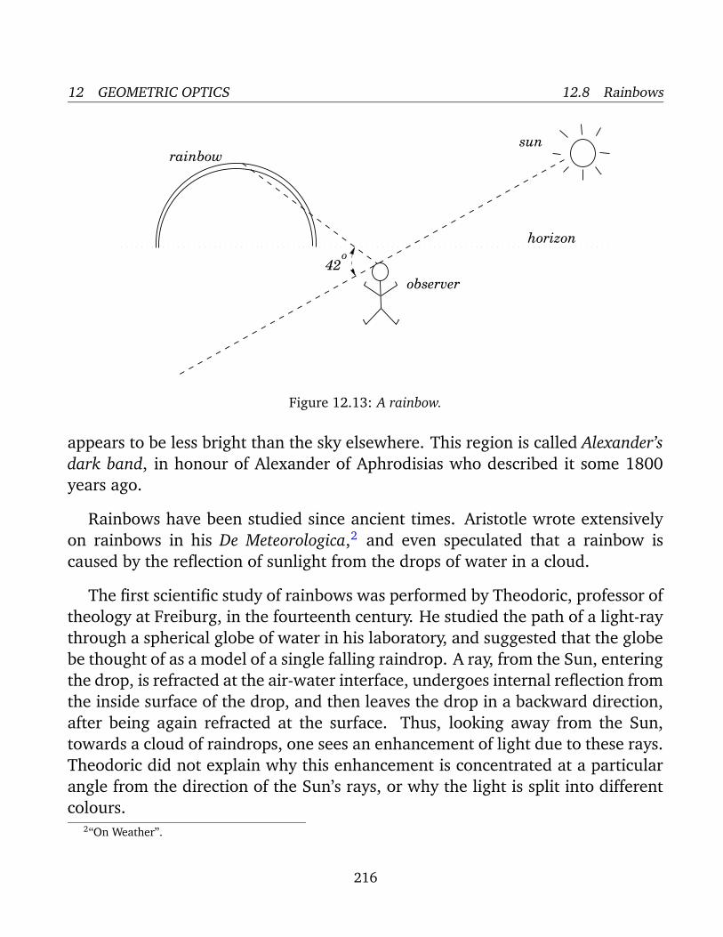
12 GEOMETRIC OPTICS 12.8 Rainbows
rainbowsun
observer
o42
horizon
Figure 12.13: A rainbow.
appears to be less bright than the sky elsewhere. This region is called Alexander’s
dark band, in honour of Alexander of Aphrodisias who described it some 1800
years ago.
Rainbows have been studied since ancient times. Aristotle wrote extensively
on rainbows in his De Meteorologica,2 and even speculated that a rainbow is
caused by the reflection of sunlight from the drops of water in a cloud.
The first scientific study of rainbows was performed by Theodoric, professor of
theology at Freiburg, in the fourteenth century. He studied the path of a light-ray
through a spherical globe of water in his laboratory, and suggested that the globe
be thought of as a model of a single falling raindrop. A ray, from the Sun, entering
the drop, is refracted at the air-water interface, undergoes internal reflection from
the inside surface of the drop, and then leaves the drop in a backward direction,
after being again refracted at the surface. Thus, looking away from the Sun,
towards a cloud of raindrops, one sees an enhancement of light due to these rays.
Theodoric did not explain why this enhancement is concentrated at a particular
angle from the direction of the Sun’s rays, or why the light is split into different
colours.2“On Weather”.
216

12 GEOMETRIC OPTICS 12.8 Rainbows
The first person to give a full explanation of how a rainbow is formed was
Rene Descartes. He showed mathematically that if one traces the path through a
spherical raindrop of parallel light-rays entering the drop at different points on
its surface, each emerges in a different direction, but there is a concentration of
emerging rays at an angle of 42 from the reverse direction to the incident rays, in
exact agreement with the observed angular size of rainbows. Furthermore, since
some colours are refracted more than others in a raindrop, the “rainbow angle”
is slightly different for each colour, so a raindrop disperses the Sun’s light into a
set of nearly overlapping coloured arcs.
Figure 12.13 illustrated Descartes’ theory in more detail. It shows parallel
light-rays entering a spherical raindrop. Only rays entering the upper half con-
tribute to the rainbow effect. Let us follow the rays, one by one, from the top
down to the middle of the drop. We observe the following pattern. Rays which
enter near the top of the drop emerge going in almost the reverse direction, but
a few degrees below the horizontal. Rays entering a little further below the top
emerge at a greater angle below the horizontal. Eventually, we reach a critical
ray, called the rainbow ray, which emerges in an angle 42 below the horizontal.
Rays entering the drop lower than the rainbow ray emerge at an angle less than
42. Thus, the rainbow ray is the one which deviates most from the reverse di-
rection to the incident rays. This variation, with 42 being the maximum angle
of deviation from the reverse direction, leads to a bunching of rays at that angle,
and, hence, to an unusually bright arc of reflected light centred around 42 from
the reverse direction. The arc has a sharp outer edge, since reflected light cannot
deviate by more than 42 from the reverse direction, and a diffuse inner edge,
since light can deviate by less than 42 from the reverse direction: 42 is just
the most likely angle of deviation. Finally, since the rainbow angle varies slightly
with wavelength (because the refractive index of water varies slightly with wave-
length), the arcs corresponding to each colour appear at slightly different angles
relative to the reverse direction to the incident rays. We expect violet light to be
refracted more strongly than red light in a raindrop. It is, therefore, clear, from
Fig. 12.14, that the red arc deviates slightly more from the reverse direction to
the incident rays than the violet arc. In other words, violet is concentrated on the
inside of the rainbow, and red is concentrated on the outside.
217

12 GEOMETRIC OPTICS 12.8 Rainbows
Figure 12.14: Descarte’s theory of the rainbow.
Descartes was also able to show that light-rays which are internally reflected
twice inside a raindrop emerge concentrated at an angle of 50 from the reverse
direction to the incident rays. Of course, this angle corresponds exactly to the
angular size of the secondary rainbow sometimes seen outside the first. This
rainbow is naturally less intense than the primary rainbow, since a light-ray loses
some of its intensity at each reflection or refraction event. Note that 50 repre-
sents the angle of maximum deviation of doubly reflected light from the reverse
direction (i.e., doubly reflected light can deviate by more than this angle, but not
by less). Thus, we expect the secondary rainbow to have a diffuse outer edge,
and a sharp inner edge. We also expect doubly reflected violet light to be re-
fracted more strongly in a raindrop than doubly reflected red light. It follows,
from Fig. 12.15, that the red secondary arc deviates slightly less from the reverse
direction to the incident rays than the violet secondary arc. In other words, red
is concentrated on the inside of the secondary rainbow, and violet on the outside.
Since no reflected light emerges between the primary and secondary rainbows
(i.e., in the angular range 42 to 50, relative to the reverse direction), we nat-
urally expect this region of the sky to look slightly less bright than the other
218

12 GEOMETRIC OPTICS 12.9 Worked Examples
Figure 12.15: Rainbow rays for the primary and secondary arcs of a rainbow.
surrounding regions of the sky, which explains Alexander’s dark band.
12.9 Worked Examples
Example 12.1: The corner-cube reflector
Question: Two mirrors are placed at right-angles to one another. Show that a
light-ray incident from any direction in the plane perpendicular to both mirrors
is reflected through 180.
Answer: Consider the diagram. We are effectively being asked to prove that
α = i1, for any value of i1. Now, from trigonometry,
i2 = 90 − r1.
But, from the law of reflection, r1 = i1 and i2 = r2, so
r2 = 90 − i1.
219

12 GEOMETRIC OPTICS 12.9 Worked Examples
i r
α
α
r
i
1 1
2
2light-ray
mirror
mirror
Trigonometry also yields
α = 90 − r2.
It follows from the previous two equations that
α = 90 − (90 − i1) = i1.
Hence, α = i1, for all values of i1.
It can easily be appreciated that a combination of three mutually perpendic-
ular mirrors would reflect a light-ray incident from any direction through 180.Such a combination of mirrors is called a corner-cube reflector. Astronauts on the
Apollo 11 mission (1969) left a panel of corner-cube reflectors on the surface of
the Moon. These reflectors have been used ever since to measure the Earth-Moon
distance via laser range finding (basically, a laser beam is fired from the Earth,
reflects off the corner-cube reflectors on the Moon, and then returns to the Earth.
The time of travel of the beam can easily be converted into the Earth-Moon dis-
tance). The Earth-Moon distance can be measured to within an accuracy of 3 cm
using this method.
220

12 GEOMETRIC OPTICS 12.9 Worked Examples
Example 12,2: Refraction
Question: A light-ray of wavelength λ1 = 589 nm traveling through air is inci-
dent on a smooth, flat slab of crown glass (refractive index 1.52) at an angle of
θ1 = 30.0 to the normal. What is the angle of refraction? What is the wave-
length λ2 of the light inside the glass? What is the frequency f of the light inside
the glass?
Answer: Snell’s law can be written
sin θ2 =n1
n2
sin θ1.
In this case, θ1 = 30, n1 ' 1.00 (here, we neglect the slight deviation of the
refractive index of air from that of a vacuum), and n2 = 1.52. Thus,
sin θ2 =(1.00)
(1.52)(0.5) = 0.329,
giving
θ2 = 19.2
as the angle of refraction (measured with respect to the normal).
The wavelength λ2 of the light inside the glass is given by
λ2 =n1
n2
λ1 =(1.00)
(1.52)(589) = 387.5 nm.
The frequency f of the light inside the glass is exactly the same as the frequency
outside the glass, and is given by
f =c
n1 λ1
=(3 × 10⁸)
(1.00) (589 × 10−9)= 5.09 × 10¹⁴ Hz.
221

13 PARAXIAL OPTICS
13 Paraxial Optics
13.1 Spherical Mirrors
A spherical mirror is a mirror which has the shape of a piece cut out of a spherical
surface. There are two types of spherical mirrors: concave, and convex. These
are illustrated in Fig. 13.1. The most commonly occurring examples of concave
mirrors are shaving mirrors and makeup mirrors. As is well-known, these types
of mirrors magnify objects placed close to them. The most commonly occurring
examples of convex mirrors are the passenger-side wing mirrors of cars. These
type of mirrors have wider fields of view than equivalent flat mirrors, but objects
which appear in them generally look smaller (and, therefore, farther away) than
they actually are.
light
reflecting surfacereflecting surface
light
Figure 13.1: A concave (left) and a convex (right) mirror
.
Let us now introduce a few key concepts which are needed to study image
formation by a concave spherical mirror. As illustrated in Fig. 13.2, the normal
to the centre of the mirror is called the principal axis. The mirror is assumed
to be rotationally symmetric about this axis. Hence, we can represent a three-
dimensional mirror in a two-dimensional diagram, without loss of generality. The
point V at which the principal axis touches the surface of the mirror is called the
222

13 PARAXIAL OPTICS 13.1 Spherical Mirrors
vertex. The point C, on the principal axis, which is equidistant from all points on
the reflecting surface of the mirror is called the centre of curvature. The distance
along the principal axis from point C to point V is called the radius of curvature
of the mirror, and is denoted R. It is found experimentally that rays striking a
concave mirror parallel to its principal axis, and not too far away from this axis,
are reflected by the mirror such that they all pass through the same point F on
the principal axis. This point, which is lies between the centre of curvature and
the vertex, is called the focal point, or focus, of the mirror. The distance along the
principal axis from the focus to the vertex is called the focal length of the mirror,
and is denoted f.
principal axis CV
F
f
R
reflecting surface
light−ray
Figure 13.2: Image formation by a concave mirror.
In our study of concave mirrors, we are going to assume that all light-rays
which strike a mirror parallel to its principal axis (e.g., all rays emanating from a
distant object) are brought to a focus at the same point F. Of course, as mentioned
above, this is only an approximation. It turns out that as rays from a distant
object depart further from the principal axis of a concave mirror they are brought
to a focus ever closer to the mirror, as shown in Fig. 13.3. This lack of perfect
focusing of a spherical mirror is called spherical aberration. The approximation
in which we neglect spherical aberration is called the paraxial approximation.3
3“Paraxial” is derived from ancient Greek roots, and means “close to the axis”.
223

13 PARAXIAL OPTICS 13.1 Spherical Mirrors
.
focuslight−ray
concave mirror
Figure 13.3: Spherical aberration in a concave mirror.
Likewise, the study of image formation under this approximation is known as
paraxial optics. This field of optics was first investigated systematically by the
famous German mathematician Karl Friedrich Gauss in 1841.
It can be demonstrated, by geometry, that the only type of mirror which does
not suffer from spherical aberration is a parabolic mirror (i.e., a mirror whose
reflecting surface is the surface of revolution of a parabola). Thus, a ray traveling
parallel to the principal axis of a parabolic mirror is brought to a focus at the
same point F, no matter how far the ray is from the axis. Since the path of a
light-ray is completely reversible, it follows that a light source placed at the focus
F of a parabolic mirror yields a perfectly parallel beam of light, after the light
has reflected off the surface of the mirror. Parabolic mirrors are more difficult,
and, therefore, more expensive, to make than spherical mirrors. Thus, parabolic
mirrors are only used in situations where the spherical aberration of a conven-
tional spherical mirror would be a serious problem. The receiving dishes of radio
telescopes are generally parabolic. They reflect the incoming radio waves from
(very) distant astronomical sources, and bring them to a focus at a single point,
where a detector is placed. In this case, since the sources are extremely faint, it
is imperative to avoid the signal losses which would be associated with spheri-
cal aberration. A car headlight consists of a light-bulb placed at the focus of a
224

13 PARAXIAL OPTICS 13.2 Image Formation by Concave Mirrors
parabolic reflector. The use of a parabolic reflector enables the headlight to cast
a very straight beam of light ahead of the car. The beam would be nowhere near
as well-focused were a spherical reflector used instead.
13.2 Image Formation by Concave Mirrors
There are two alternative methods of locating the image formed by a concave
mirror. The first is purely graphical, and the second uses simple algebraic analy-
sis.
The graphical method of locating the image produced by a concave mirror con-
sists of drawing light-rays emanating from key points on the object, and finding
where these rays are brought to a focus by the mirror. This task can be accom-
plished using just four simple rules:
1. An incident ray which is parallel to the principal axis is reflected through the
focus F of the mirror.
2. An incident ray which passes through the focus F of the mirror is reflected
parallel to the principal axis.
3. An incident ray which passes through the centre of curvature C of the mirror
is reflected back along its own path (since it is normally incident on the
mirror).
4. An incident ray which strikes the mirror at its vertex V is reflected such that
its angle of incidence with respect to the principal axis is equal to its angle
of reflection.
The validity of these rules in the paraxial approximation is fairly self-evident.
Consider an object ST which is placed a distance p from a concave spherical
mirror, as shown in Fig. 13.4. For the sake of definiteness, let us suppose that the
object distance p is greater than the focal length f of the mirror. Each point on
the object is assumed to radiate light-rays in all directions. Consider four light-
rays emanating from the tip T of the object which strike the mirror, as shown
225

13 PARAXIAL OPTICS 13.2 Image Formation by Concave Mirrors
S’
T
SC F
T’
V
4
3
1
2
p
q
Figure 13.4: Formation of a real image by a concave mirror.
in the figure. The reflected rays are constructed using rules 1–4 above, and the
rays are labelled accordingly. It can be seen that the reflected rays all come
together at some point T ′. Thus, T ′ is the image of T (i.e., if we were to place
a small projection screen at T ′ then we would see an image of the tip on the
screen). As is easily demonstrated, rays emanating from other parts of the object
are brought into focus in the vicinity of T ′ such that a complete image of the
object is produced between S ′ and T ′ (obviously, point S ′ is the image of point
S). This image could be viewed by projecting it onto a screen placed between
points S ′ and T ′. Such an image is termed a real image. Note that the image S ′T ′
would also be directly visible to an observer looking straight at the mirror from
a distance greater than the image distance q (since the observer’s eyes could not
tell that the light-rays diverging from the image were in anyway different from
those which would emanate from a real object). According to the figure, the
image is inverted with respect to the object, and is also magnified.
Figure 13.5 shows what happens when the object distance p is less than the
focal length f. In this case, the image appears to an observer looking straight at
the mirror to be located behind the mirror. For instance, rays emanating from
226

13 PARAXIAL OPTICS 13.2 Image Formation by Concave Mirrors
C F
S’
T’2
3V
S
T
Figure 13.5: Formation of a virtual image by a concave mirror.
the tip T of the object appear, after reflection from the mirror, to come from a
point T ′ which is behind the mirror. Note that only two rays are used to locate
T ′, for the sake of clarity. In fact, two is the minimum number of rays needed to
locate a point image. Of course, the image behind the mirror cannot be viewed
by projecting it onto a screen, because there are no real light-rays behind the
mirror. This type of image is termed a virtual image. The characteristic difference
between a real image and a virtual image is that, immediately after reflection
from the mirror, light-rays emitted by the object converge on a real image, but
diverge from a virtual image. According to Fig. 13.5, the image is upright with
respect to the object, and is also magnified.
The graphical method described above is fine for developing an intuitive un-
derstanding of image formation by concave mirrors, or for checking a calculation,
but is a bit too cumbersome for everyday use. The analytic method described be-
low is far more flexible.
Consider an object ST placed a distance p in front of a concave mirror of radius
of curvature R. In order to find the image S ′T ′ produced by the mirror, we draw
two rays from T to the mirror—see Fig. 13.6. The first, labelled 1, travels from T
to the vertex V and is reflected such that its angle of incidence θ equals its angle
227

13 PARAXIAL OPTICS 13.2 Image Formation by Concave Mirrors
S
T
S’CVθ
θ
B
h2
1
p
R
q
αα h’
T’
Figure 13.6: Image formation by a concave mirror.
of reflection. The second ray, labelled 2, passes through the centre of curvature
C of the mirror, strikes the mirror at point B, and is reflected back along its own
path. The two rays meet at point T ′. Thus, S ′T ′ is the image of ST , since point S ′
must lie on the principal axis.
In the triangle STV , we have tan θ = h/p, and in the triangle S ′T ′V we have
tan θ = −h ′/q, where p is the object distance, and q is the image distance. Here,
h is the height of the object, and h ′ is the height of the image. By convention, h ′
is a negative number, since the image is inverted (if the image were upright then
h ′ would be a positive number). It follows that
tan θ =h
p=
−h ′
q. (13.1)
Thus, the magnification M of the image with respect to the object is given by
M =h ′
h= −
q
p. (13.2)
By convention, M is negative if the image is inverted with respect to the object,
and positive if the image is upright. It is clear that the magnification of the image
is just determined by the ratio of the image and object distances from the vertex.
228

13 PARAXIAL OPTICS 13.2 Image Formation by Concave Mirrors
From triangles STC and S ′T ′C, we have tan α = h/(p − R) and tan α =
−h ′/(R − q), respectively. These expressions yield
tan α =h
p − R= −
h ′
R − q. (13.3)
Equations (13.2) and (13.3) can be combined to give
−h ′
h=
R − q
p − R=
q
p, (13.4)
which easily reduces to1
p+
1
q=
2
R. (13.5)
This expression relates the object distance, the image distance, and the radius of
curvature of the mirror.
For an object which is very far away from the mirror (i.e., p → ∞), so that
light-rays from the object are parallel to the principal axis, we expect the image
to form at the focal point F of the mirror. Thus, in this case, q = f, where f is the
focal length of the mirror, and Eq. (13.5) reduces to
0 +1
f=
2
R. (13.6)
The above expression yields
f =R
2. (13.7)
In other words, in the paraxial approximation, the focal length of a concave
spherical mirror is half of its radius of curvature. Equations (13.5) and (13.7)
can be combined to give1
p+
1
q=
1
f. (13.8)
The above expression was derived for the case of a real image. However, as is
easily demonstrated, it also applies to virtual images provided that the following
sign convention is adopted. For real images, which always form in front of the
mirror, the image distance q is positive. For virtual images, which always form
229
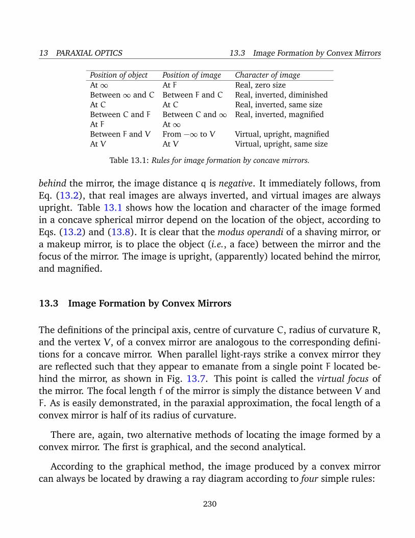
13 PARAXIAL OPTICS 13.3 Image Formation by Convex Mirrors
Position of object Position of image Character of image
At ∞ At F Real, zero size
Between ∞ and C Between F and C Real, inverted, diminished
At C At C Real, inverted, same size
Between C and F Between C and ∞ Real, inverted, magnified
At F At ∞Between F and V From −∞ to V Virtual, upright, magnified
At V At V Virtual, upright, same size
Table 13.1: Rules for image formation by concave mirrors.
behind the mirror, the image distance q is negative. It immediately follows, from
Eq. (13.2), that real images are always inverted, and virtual images are always
upright. Table 13.1 shows how the location and character of the image formed
in a concave spherical mirror depend on the location of the object, according to
Eqs. (13.2) and (13.8). It is clear that the modus operandi of a shaving mirror, or
a makeup mirror, is to place the object (i.e., a face) between the mirror and the
focus of the mirror. The image is upright, (apparently) located behind the mirror,
and magnified.
13.3 Image Formation by Convex Mirrors
The definitions of the principal axis, centre of curvature C, radius of curvature R,
and the vertex V , of a convex mirror are analogous to the corresponding defini-
tions for a concave mirror. When parallel light-rays strike a convex mirror they
are reflected such that they appear to emanate from a single point F located be-
hind the mirror, as shown in Fig. 13.7. This point is called the virtual focus of
the mirror. The focal length f of the mirror is simply the distance between V and
F. As is easily demonstrated, in the paraxial approximation, the focal length of a
convex mirror is half of its radius of curvature.
There are, again, two alternative methods of locating the image formed by a
convex mirror. The first is graphical, and the second analytical.
According to the graphical method, the image produced by a convex mirror
can always be located by drawing a ray diagram according to four simple rules:
230

13 PARAXIAL OPTICS 13.3 Image Formation by Convex Mirrors
light-ray
F C
f
R
V
Figure 13.7: The virtual focus of a convex mirror.
1. An incident ray which is parallel to the principal axis is reflected as if it came
from the virtual focus F of the mirror.
2. An incident ray which is directed towards the virtual focus F of the mirror is
reflected parallel to the principal axis.
3. An incident ray which is directed towards the centre of curvature C of the
mirror is reflected back along its own path (since it is normally incident on
the mirror).
4. An incident ray which strikes the mirror at its vertex V is reflected such that
its angle of incidence with respect to the principal axis is equal to its angle
of reflection.
The validity of these rules in the paraxial approximation is, again, fairly self-
evident.
In the example shown in Fig. 13.8, two rays are used to locate the image S ′T ′
of an object ST placed in front of the mirror. It can be seen that the image is
virtual, upright, and diminished.
231

13 PARAXIAL OPTICS 13.3 Image Formation by Convex Mirrors
S S’
T’
F C
T
3
1
Figure 13.8: Image formation by a convex mirror.
Position of object Position of image Character of image
At ∞ At F Virtual, zero size
Between ∞ and V Between F and V Virtual, upright, diminished
At V At V Virtual, upright, same size
Table 13.2: Rules for image formation by convex mirrors.
As is easily demonstrated, application of the analytical method to image for-
mation by convex mirrors again yields Eq. (13.2) for the magnification of the
image, and Eq. (13.8) for the location of the image, provided that we adopt the
following sign convention. The focal length f of a convex mirror is redefined to
be minus the distance between points V and F. In other words, the focal length
of a concave mirror, with a real focus, is always positive, and the focal length of a
convex mirror, with a virtual focus, is always negative. Table 13.2 shows how the
location and character of the image formed in a convex spherical mirror depend
on the location of the object, according to Eqs. (13.2) and (13.8) (with f < 0).
In summary, the formation of an image by a spherical mirror involves the
crossing of light-rays emitted by the object and reflected off the mirror. If the
light-rays actually cross in front of the mirror then the image is real. If the light-
rays do not actually cross, but appear to cross when projected backwards behind
the mirror, then the image is virtual. A real image can be projected onto a screen,
232

13 PARAXIAL OPTICS 13.4 Image Formation by Plane Mirrors
a virtual image cannot. However, both types of images can be seen by an observer,
and photographed by a camera. The magnification of the image is specified by
Eq. (13.2), and the location of the image is determined by Eq. (13.8). These
two formulae can be used to characterize both real and virtual images formed by
either concave or convex mirrors, provided that the following sign conventions
are observed:
1. The height h ′ of the image is positive if the image is upright, with respect to
the object, and negative if the image is inverted.
2. The magnification M of the image is positive if the image is upright, with
respect to the object, and negative if the image is inverted.
3. The image distance q is positive if the image is real, and, therefore, located
in front of the mirror, and negative if the image is virtual, and, therefore,
located behind the mirror.
4. The focal length f of the mirror is positive if the mirror is concave, so that
the focal point F is located in front of the mirror, and negative if the mirror
is convex, so that the focal point F is located behind the mirror.
Note that the front side of the mirror is defined to be the side from which the
light is incident.
13.4 Image Formation by Plane Mirrors
Both concave and convex spherical mirrors asymptote to plane mirrors in the
limit in which their radii of curvature R tend to infinity. In other words, a plane
mirror can be treated as either a concave or a convex mirror for which R → ∞.
Now, if R → ∞, then f = ±R/2 → ∞, so 1/f → 0, and Eq. (13.8) yields
1
p+
1
q=
1
f= 0, (13.9)
or
q = −p. (13.10)
233

13 PARAXIAL OPTICS 13.5 Thin Lenses
O
optic axis
lens
Figure 13.9: The optic axis of a lens.
Thus, for a plane mirror the image is virtual, and is located as far behind the
mirror as the object is in front of the mirror. According to Eq. (13.2), the magni-
fication of the image is given by
M = −q
p= 1. (13.11)
Clearly, the image is upright, since M > 0, and is the same size as the object, since
|M| = 1. However, an image seen in a plane mirror does differ from the original
object in one important respect: i.e., left and right are swapped over. In other
words, a right-hand looks like a left-hand in a plane mirror, and vice versa.
13.5 Thin Lenses
A lens is a transparent medium (usually glass) bounded by two curved sur-
faces (generally either spherical, cylindrical, or plane surfaces). As illustrated
in Fig. 13.9, the line which passes normally through both bounding surfaces of
a lens is called the optic axis. The point O on the optic axis which lies midway
between the two bounding surfaces is called the optic centre.
There are two basic kinds of lenses: converging, and diverging. A converging
lens brings all incident light-rays parallel to its optic axis together at a point F,
behind the lens, called the focal point, or focus, of the lens. A diverging lens
spreads out all incident light-rays parallel to its optic axis so that they appear to
diverge from a virtual focal point F in front of the lens. Here, the front side of
the lens is conventionally defined to be the side from which the light is incident.
234

13 PARAXIAL OPTICS 13.5 Thin Lenses
O
O
F
light−ray
f
f
F
Figure 13.10: The focii of converging (top) and diverging (bottom) lens.
The differing effects of a converging and a diverging lens on incident light-rays
parallel to the optic axis (i.e., emanating from a distant object) are illustrated in
Fig. 13.10.
Lenses, like mirrors, suffer from spherical aberration, which causes light-rays
parallel to the optic axis, but a relatively long way from the axis, to be brought
to a focus, or a virtual focus, closer to the lens than light-rays which are relatively
close to the axis. It turns out that spherical aberration in lenses can be completely
cured by using lenses whose bounding surfaces are non-spherical. However, such
lenses are more difficult, and, therefore, more expensive, to manufacture than
conventional lenses whose bounding surfaces are spherical. Thus, the former sort
of lens is only employed in situations where the spherical aberration of a conven-
tional lens would be a serious problem. The usual method of curing spherical
aberration is to use combinations of conventional lenses (i.e., compound lenses).
In the following, we shall make use of the paraxial approximation, in which spher-
ical aberration is completely ignored, and all light-rays parallel to the optic axis
235

13 PARAXIAL OPTICS 13.5 Thin Lenses
O
Cb fC
Rb Rf
light-ray
Figure 13.11: A thin lens.
are assumed to be brought to a focus, or a virtual focus, at the same point F. This
approximation is valid as long as the radius of the lens is small compared to the
object distance and the image distance.
The focal length of a lens, which is usually denoted f, is defined as the distance
between the optic centre O and the focal point F, as shown in Fig. 13.10. How-
ever, by convention, converging lenses have positive focal lengths, and diverging
lenses have negative focal lengths. In other words, if the focal point lies behind
the lens then the focal length is positive, and if the focal point lies in front of the
lens then the focal length is negative.
Consider a conventional lens whose bounding surfaces are spherical. Let Cf
be the centre of curvature of the front surface, and Cb the centre of curvature of
the back surface. The radius of curvature Rf of the front surface is the distance
between the optic centre O and the point Cf. Likewise, the radius of curvature
Rb of the back surface is the distance between points O and Cb. However, by
convention, the radius of curvature of a bounding surface is positive if its centre
of curvature lies behind the lens, and negative if its centre of curvature lies in front
of the lens. Thus, in Fig. 13.11, Rf is positive and Rb is negative.
In the paraxial approximation, it is possible to find a simple formula relating
the focal length f of a lens to the radii of curvature, Rf and Rb, of its front and
236

13 PARAXIAL OPTICS 13.5 Thin Lenses
back bounding surfaces. This formula is written
1
f= (n − 1)
(
1
Rf
−1
Rb
)
, (13.12)
where n is the refractive index of the lens. The above formula is usually called the
lens-maker’s formula, and was discovered by Descartes. Note that the lens-maker’s
formula is only valid for a thin lens whose thickness is small compared to its focal
length. What Eq. (13.12) is basically telling us is that light-rays which pass from
air to glass through a convex surface are focused, whereas light-rays which pass
from air to glass through a concave surface are defocused. Furthermore, since
light-rays are reversible, it follows that rays which pass from glass to air through
a convex surface are defocused, whereas rays which pass from air to glass through
a concave surface are focused. Note that the net focusing or defocusing action of a
lens is due to the difference in the radii of curvature of its two bounding surfaces.
Suppose that a certain lens has a focal length f. What happens to the focal
length if we turn the lens around, so that its front bounding surface becomes
its back bounding surface, and vice versa? It is easily seen that when the lens
is turned around Rf → −Rb and Rb → −Rf. However, the focal length f of the
lens is invariant under this transformation, according to Eq. (13.12). Thus, the
focal length of a lens is the same for light incident from either side. In particular, a
converging lens remains a converging lens when it is turned around, and likewise
for a diverging lens.
The most commonly occurring type of converging lens is a bi-convex, or double-
convex, lens, for which Rf > 0 and Rb < 0. In this type of lens, both bounding
surfaces have a focusing effect on light-rays passing through the lens. Another
fairly common type of converging lens is a plano-convex lens, for which Rf > 0 and
Rb = ∞. In this type of lens, only the curved bounding surface has a focusing
effect on light-rays. The plane surface has no focusing or defocusing effect. A
less common type of converging lens is a convex-meniscus lens, for which Rf > 0
and Rb > 0, with Rf < Rb. In this type of lens, the front bounding surface has a
focusing effect on light-rays, whereas the back bounding surface has a defocusing
effect, but the focusing effect of the front surface wins out.
The most commonly occurring type of diverging lens is a bi-concave, or double-
237

13 PARAXIAL OPTICS 13.5 Thin Lenses
concave, lens, for which Rf < 0 and Rb > 0. In this type of lens, both bounding
surfaces have a defocusing effect on light-rays passing through the lens. Another
fairly common type of converging lens is a plano-concave lens, for which Rf <
0 and Rb = ∞. In this type of lens, only the curved bounding surface has a
defocusing effect on light-rays. The plane surface has no focusing or defocusing
effect. A less common type of converging lens is a concave-meniscus lens, for
which Rf < 0 and Rb < 0, with Rf < |Rb|. In this type of lens, the front bounding
surface has a defocusing effect on light-rays, whereas the back bounding surface
has a focusing effect, but the defocusing effect of the front surface wins out.
Figure 13.12 shows the various types of lenses mentioned above. Note that,
as a general rule, converging lenses are thicker at the centre than at the edges,
whereas diverging lenses are thicker at the edges than at the centre.
convex-meniscusbi-convex plano-convex
bi-concave concave-meniscusplano-concave
Figure 13.12: Various different types of thin lens.
238

13 PARAXIAL OPTICS 13.6 Image Formation by Thin Lenses
13.6 Image Formation by Thin Lenses
There are two alternative methods of locating the image formed by a thin lens.
Just as for spherical mirrors, the first method is graphical, and the second analyt-
ical.
The graphical method of locating the image formed by a thin lens involves
drawing light-rays emanating from key points on the object, and finding where
these rays are brought to a focus by the lens. This task can be accomplished using
a small number of simple rules.
Consider a converging lens. It is helpful to define two focal points for such a
lens. The first, the so-called image focus, denoted Fi, is defined as the point behind
the lens to which all incident light-rays parallel to the optic axis converge after
passing through the lens. This is the same as the focal point F defined previously.
The second, the so-called object focus, denoted Fo, is defined as the position in
front of the lens for which rays emitted from a point source of light placed at
that position would be refracted parallel to the optic axis after passing through
the lens. It is easily demonstrated that the object focus Fo is as far in front of the
optic centre O of the lens as the image focus Fi is behind O. The distance from
the optic centre to either focus is, of course, equal to the focal length f of the lens.
The image produced by a converging lens can be located using just three simple
rules:
1. An incident ray which is parallel to the optic axis is refracted through the
image focus Fi of the lens.
2. An incident ray which passes through the object focus Fo of the lens is re-
fracted parallel to the optic axis.
3. An incident ray which passes through the optic centre O of the lens is not
refracted at all.
The last rule is only an approximation. It turns out that although a light-ray
which passes through the optic centre of the lens does not change direction, it is
239

13 PARAXIAL OPTICS 13.6 Image Formation by Thin Lenses
displaced slightly to one side. However, this displacement is negligible for a thin
lens.
Figure 13.13 illustrates how the image S ′T ′ of an object ST placed in front
of a converging lens is located using the above rules. In fact, the three rays,
1–3, emanating from the tip T of the object, are constructed using rules 1–3,
respectively. Note that the image is real (since light-rays actually cross), inverted,
and diminished.
f f
1
3
2
T
S
T’
S’Fo
FiO
Figure 13.13: Image formation by a converging lens.
Consider a diverging lens. It is again helpful to define two focal points for
such a lens. The image focus Fi is defined as the point in front of the lens from
which all incident light-rays parallel to the optic axis appear to diverge after
passing through the lens. This is the same as the focal point F defined earlier.
The object focus Fo is defined as the point behind the lens to which all incident
light-rays which are refracted parallel to the optic axis after passing through the
lens appear to converge. Both foci are located a distance f from the optic centre,
where f is the focal length of the lens. The image produced by a diverging lens
can be located using the following three rules:
1. An incident ray which is parallel to the optic axis is refracted as if it came
from the image focus Fi of the lens.
240

13 PARAXIAL OPTICS 13.6 Image Formation by Thin Lenses
S
T
S’
T’
O
Fi oF
12
3
f f
Figure 13.14: Image formation by a diverging lens.
2. An incident ray which is directed towards the object focus Fo of the lens is
refracted parallel to the optic axis.
3. An incident ray which passes through the optic centre O of the lens is not
refracted at all.
Figure 13.14 illustrates how the image S ′T ′ of an object ST placed in front of
a diverging lens is located using the above rules. In fact, the three rays, 1–3, em-
anating from the tip T of the object, are constructed using rules 1–3, respectively.
Note that the image is virtual (since light-rays do not actually cross), upright, and
diminished.
Let us now investigate the analytical method. Consider an object of height h
placed a distance p in front of a converging lens. Suppose that a real image of
height h ′ is formed a distance q behind the lens. As is illustrated in Fig. 13.15,
the image can be located using rules 1 and 3, discussed above.
Now, the right-angled triangles SOT and S ′OT ′ are similar, so
−h ′
h=
OS ′
OS=
q
p. (13.13)
241

13 PARAXIAL OPTICS 13.6 Image Formation by Thin Lenses
SF
T
O
P
f
h
h’
1
3
pq
S’
T’
Figure 13.15: Image formation by a converging lens.
Here, we have adopted the convention that the image height h ′ is negative if the
image is inverted. The magnification of a thin converging lens is given by
M =h ′
h= −
q
p. (13.14)
This is the same as the expression (13.2) for the magnification of a spherical
mirror. Note that we are again adopting the convention that the magnification is
negative if the image is inverted.
The right-angled triangles OPF and S ′T ′F are also similar, and so
S ′T ′
OP=
FS ′
OF, (13.15)
or−h ′
h=
q
p=
q − f
f. (13.16)
The above expression can be rearranged to give
1
p+
1
q=
1
f. (13.17)
Note that this is exactly the same as the formula (13.8) relating the image and
object distances in a spherical mirror.
242

13 PARAXIAL OPTICS 13.6 Image Formation by Thin Lenses
Position of object Position of image Character of image
At +∞ At F Real, zero size
Between +∞ and Vo Between F and Vi Real, inverted, diminished
At Vo At Vi Real, inverted, same size
Between Vo and F Between Vi and −∞ Real, inverted, magnified
At F At −∞Between F and O From +∞ to O Virtual, upright, magnified
At O At O Virtual, upright, same size
Table 13.3: Rules for image formation by converging lenses.
Position of object Position of image Character of image
At ∞ At Fi Virtual, zero size
Between ∞ and O Between Fi and O Virtual, upright, diminished
At O At O Virtual, upright, same size
Table 13.4: Rules for image formation by diverging lenses.
Although formulae (13.14) and (13.17) were derived for the case of a real
image formed by a converging lens, they also apply to virtual images, and to
images formed by diverging lenses, provided that the following sign conventions
are adopted. First of all, as we have already mentioned, the focal length f of
a converging lens is positive, and the focal length of a diverging lens is negative.
Secondly, the image distance q is positive if the image is real, and, therefore,
located behind the lens, and negative if the image is virtual, and, therefore, located
in front of the lens. It immediately follows, from Eq. (13.14), that real images are
always inverted, and virtual images are always upright.
Table 13.3 shows how the location and character of the image formed by a
converging lens depend on the location of the object. Here, the point Vo is located
on the optic axis two focal lengths in front of the optic centre, and the point Vi
is located on the optic axis two focal lengths behind the optic centre. Note the
almost exact analogy between the image forming properties of a converging lens
and those of a concave spherical mirror.
Table 13.4 shows how the location and character of the image formed by a di-
verging lens depend on the location of the object. Note the almost exact analogy
between the image forming properties of a diverging lens and those of a convex
spherical mirror.
243

13 PARAXIAL OPTICS 13.7 Chromatic aberration
Finally, let us reiterate the sign conventions used to determine the positions
and characters of the images formed by thin lenses:
1. The height h ′ of the image is positive if the image is upright, with respect to
the object, and negative if the image is inverted.
2. The magnification M of the image is positive if the image is upright, with
respect to the object, and negative if the image is inverted.
3. The image distance q is positive if the image is real, and, therefore, located
behind the lens, and negative if the image is virtual, and, therefore, located
in front of the lens.
4. The focal length f of the lens is positive if the lens is converging, so that
the image focus Fi is located behind the lens, and negative if the lens is
diverging, so that the image focus Fi is located in front of the lens.
Note that the front side of the lens is defined to be the side from which the light
is incident.
13.7 Chromatic aberration
We have seen that both mirrors and lenses suffer from spherical aberration, an ef-
fect which limits the clarity and sharpness of the images formed by such devices.
However, lenses also suffer from another type of abberation called chromatic ab-
beration. This occurs because the index of refraction of the glass in a lens is
different for different wavelengths. We have seen that a prism refracts violet
light more than red light. The same is true of lenses. As a result, a simple lens
focuses violet light closer to the lens than it focuses red light. Hence, white light
produces a slightly blurred image of an object, with coloured edges.
For many years, chromatic abberation was a sufficiently serious problem for
lenses that scientists tried to find ways of reducing the number of lenses in scien-
tific instruments, or even eliminating them all together. For instance, Isaac New-
ton developed a type of telescope, now called the Newtonian telescope, which
244

13 PARAXIAL OPTICS 13.8 Worked Examples
uses a mirror instead of a lens to collect light. However, in 1758, John Dol-
lond, an English optician, discovered a way to eliminate chromatic abberation.
He combined two lenses, one converging, the other diverging, to make an achro-
matic doublet. The two lenses in an achromatic doublet are made of different
type of glass with indices of refraction chosen such that the combination brings
any two chosen colours to the same sharp focus.
Modern scientific instruments use compound lenses (i.e., combinations of sim-
ple lenses) to simultaneously eliminate both chromatic and spherical aberration.
13.8 Worked Examples
Example 13.1: Concave mirrors
Question: An object of height h = 4 cm is placed a distance p = 15 cm in front of
a concave mirror of focal length f = 20 cm. What is the height, location, and na-
ture of the image? Suppose that the object is moved to a new position a distance
p = 25 cm in front of the mirror. What now is the height, location, and nature of
the image?
Answer: According to Eq. (13.8), the image distance q is given by
q =1
1/f − 1/p=
1
(1/20 − 1/15)= −60 cm.
Thus, the image is virtual (since q < 0), and is located 60 cm behind the mirror.
According to Eq. (13.2), the magnification M of the image is given by
M = −q
p= −
(−60)
(15)= 4.
Thus, the image is upright (since M > 0), and magnified by a factor of 4. It
follows that the height h ′ of the image is given by
h ′ = M h = (4) (4) = 16 cm.
245

13 PARAXIAL OPTICS 13.8 Worked Examples
If the object is moved such that p = 25 cm then the new image distance is
given by
q =1
1/f − 1/p=
1
(1/20 − 1/25)= 100 cm.
Thus, the new image is real (since q > 0), and is located 100 cm in front of the
mirror. The new magnification is given by
M = −q
p= −
(100)
(15)= −6.67.
Thus, the image is inverted (since M < 0), and magnified by a factor of 6.67. It
follows that the new height of the image is
h ′ = M h = −(6.67) (4) = −26.67 cm.
Note that the height is negative because the image is inverted.
Example 13.2: Convex mirrors
Question: How far must an object be placed in front of a convex mirror of radius
of curvature R = 50 cm in order to ensure that the size of the image is ten times
less than the size of the object? How far behind the mirror is the image located?
Answer: The focal length f of a convex mirror is minus half of its radius of cur-
vature (taking the sign convention for the focal lengths of convex mirrors into
account). Thus, f = −25 cm. If the image is ten times smaller than the object
then the magnification is M = 0.1. We can be sure that M = +0.1, as opposed to
−0.1, because we know that images formed in convex mirrors are always virtual
and upright. According to Eq. (13.2), the image distance q is given by
q = −M p,
where p is the object distance. This can be combined with Eq. (13.8) to give
p = f
(
1 −1
M
)
= −(25) (1 − 10) = 225 cm.
246

13 PARAXIAL OPTICS 13.8 Worked Examples
Thus, the object must be placed 225 cm in front of the mirror. The image distance
is given by
q = −M p = −(0.1) (225) = −22.5 cm.
Thus, the image is located 22.5 cm behind the mirror.
Example 13.3: Converging lenses
Question: An object of height h = 7 cm is placed a distance p = 25 cm in front
of a thin converging lens of focal length f = 35 cm. What is the height, location,
and nature of the image? Suppose that the object is moved to a new location a
distance p = 90 cm in front of the lens. What now is the height, location, and
nature of the image?
Answer: According to Eq. (13.17), the image distance q is given by
q =1
1/f − 1/p=
1
(1/35 − 1/25)= −87.5 cm.
Thus, the image is virtual (since q < 0), and is located 87.5 cm in front of the
lens. According to Eq. (10.24), the magnification M of the image is given by
M = −q
p= −
(−87.5)
(25)= 3.5.
Thus, the image is upright (since M > 0), and magnified by a factor of 3.5. It
follows that the height h ′ of the image is given by
h ′ = M h = (3.5) (7) = 24.5 cm.
If the object is moved such that p = 90 cm then the new image distance is
given by
q =1
1/f − 1/p=
1
(1/35 − 1/90)= 57.27 cm.
Thus, the new image is real (since q > 0), and is located 57.27 cm behind the
lens. The new magnification is given by
M = −q
p= −
(57.27)
(90)= −0.636.
247

13 PARAXIAL OPTICS 13.8 Worked Examples
Thus, the image is inverted (since M < 0), and diminished by a factor of 0.636. It
follows that the new height of the image is
h ′ = M h = −(9.636) (7) = −4.45 cm.
Note that the height is negative because the image is inverted.
Example 13.4: Diverging lenses
Question: How far must an object be placed in front of a diverging lens of focal
length 45 cm in order to ensure that the size of the image is fifteen times less than
the size of the object? How far in front of the lens is the image located?
Answer: The focal length f of a diverging lens is negative by convention, so
f = −45 cm, in this case. If the image is fifteen times smaller than the object
then the magnification is M = 0.0667. We can be sure that M = +0.0667, as
opposed to −0.0667, because we know that images formed in diverging lenses
are always virtual and upright. According to Eq. (13.14), the image distance q is
given by
q = −M p,
where p is the object distance. This can be combined with Eq. (13.17) to give
p = f
(
1 −1
M
)
= −(45) (1 − 15) = 630 cm.
Thus, the object must be placed 630 cm in front of the lens. The image distance
is given by
q = −M p = −(0.0667) (630) = −42 cm.
Thus, the image is located 42 cm in front of the lens.
248

14 WAVE OPTICS
14 Wave Optics
14.1 Introduction
Geometric optics is an incredibly successful theory. Probably its most important
application is in describing and explaining the operation of commonly occurring
optical instruments: e.g., the camera, the telescope, and the microscope. Al-
though geometric optics does not make any explicit assumption about the nature
of light, it tends to suggest that light consists of a stream of massless particles.
This is certainly what scientists, including, most notably, Isaac Newton, generally
assumed up until about the year 1800.
Let us examine how the particle theory of light accounts for the three basic
laws of geometric optics:
1. The law of geometric propagation: This is easy. Massless particles obviously
move in straight-lines in free space.
2. The law of reflection: This is also fairly easy. We merely have to assume
that light particles bounce elastically (i.e., without energy loss) off reflecting
surfaces.
3. The law of refraction: This is the tricky one. Let us assume that the speed of
light particles propagating through a transparent dielectric medium is pro-
portional to the index of refraction, n ≡√
K. Let us further assume that
at a general interface between two different dielectric media, light particles
crossing the interface conserve momentum in the plane parallel to the in-
terface. In general, this implies that the particle momenta normal to the
interface are not conserved: i.e., the interface exerts a normal reaction force
on crossing particles, but no parallel force. From Fig. 14.1, parallel momen-
tum conservation for light particles crossing the interface yields
v1 sin θ1 = v2 sin θ2. (14.1)
However, by assumption, v1 = n1 c and v2 = n2 c, so
n1 sin θ1 = n2 sin θ2. (14.2)
249

14 WAVE OPTICS 14.1 Introduction
θ2
θ1
n
n
1
v2
v
2
1
interface
normal
Figure 14.1: Descartes’ model of refraction
This highly contrived (and incorrect) derivation of the law of refraction was
first proposed by Descartes in 1637. Note that it depends crucially on the
(incorrect) assumption that light travels faster in dense media (e.g., glass)
than in rarefied media (e.g., water). This assumption appears very strange
to us nowadays, but it seemed eminently reasonable to scientists in the 17th
and 18th centuries. After all, they knew that sound travels faster in dense
media (e.g., water) than in rarefied media (e.g., air).
The wave theory of light, which became established in the first half of the
19th century, initially encountered tremendous resistance. Let us briefly examine
the reasons why scientists in the early 1800s refused to think of light as a wave
phenomenon? Firstly, the particle theory of light was intimately associated with
Isaac Newton, so any attack on this theory was considered to be a slight to his
memory. Secondly, all of the waves that scientists were familiar with at that
time manifestly did not travel in straight-lines. For instance, water waves are
diffracted as they pass through the narrow mouth of a harbour, as shown in
Fig. 14.2. In other words, the “rays” associated with such waves are bent as
they traverse the harbour mouth. Scientists thought that if light were a wave
phenomenon then it would also not travel in straight-lines: i.e., it would not
cast straight, sharp shadows, any more than water waves cast straight, sharp
“shadows.” Unfortunately, they did not appreciate that if the wavelength of light
250

14 WAVE OPTICS 14.2 Huygens’ principle
mouthharbour
water waves
diffraction
Figure 14.2: Refraction of water waves through the entrance of a harbour.
is much shorter than that of water waves then light can be a wave phenomenon
and still propagate in a largely geometric manner.
14.2 Huygens’ principle
The first person to explain how wave theory can also account for the laws of
geometric optics was Christiaan Huygens in 1670. At the time, of course, no-
body took the slightest notice of him. His work was later rediscovered after the
eventual triumph of wave theory.
Huygens had a very important insight into the nature of wave propagation
which is nowadays called Huygens’ principle. When applied to the propagation of
light waves, this principle states that:
Every point on a wave-front may be considered a source of secondary spherical
wavelets which spread out in the forward direction at the speed of light. The
new wave-front is the tangential surface to all of these secondary wavelets.
According to Huygens’ principle, a plane light wave propagates though free
251

14 WAVE OPTICS 14.3 Young’s Double-Slit Experiment
original wave-front
new wave-front
source of secondary wavelet
light ray
secondary wavelet
Figure 14.3: Huygen’s principle.
space at the speed of light, c. The light rays associated with this wave-front
propagate in straight-lines, as shown in Fig. 14.3. It is also fairly straightforward
to account for the laws of reflection and refraction using Huygens’ principle.
14.3 Young’s Double-Slit Experiment
The first serious challenge to the particle theory of light was made by the English
scientist Thomas Young in 1803. Young possessed one of the most brilliant minds
in the history of science. A physician by training, he was the first to describe
how the lens of the human eye changes shape in order to focus on objects at
differing distances. He also studied Physics, and, amongst other things, definitely
established the wave theory of light, as described below. Finally, he also studied
Egyptology, and helped decipher the Rosetta Stone.
Young knew that sound was a wave phenomenon, and, hence, that if two
sound waves of equal intensity, but 180 out of phase, reach the ear then they
cancel one another out, and no sound is heard. This phenomenon is called in-
terference. Young reasoned that if light were actually a wave phenomenon, as he
suspected, then a similar interference effect should occur for light. This line of
252

14 WAVE OPTICS 14.3 Young’s Double-Slit Experiment
d
L
narrow slits screen
metal sheetlight
Figure 14.4: Young’s double-slit experiment.
reasoning lead Young to perform an experiment which is nowadays referred to as
Young’s double-slit experiment.
In Young’s experiment, two very narrow parallel slits, separated by a distance
d, are cut into a thin sheet of metal. Monochromatic light, from a distant light-
source, passes through the slits and eventually hits a screen a comparatively large
distance L from the slits. The experimental setup is sketched in Fig. 14.4.
According to Huygens’ principle, each slit radiates spherical light waves. The
light waves emanating from each slit are superposed on the screen. If the waves
are 180 out of phase then destructive interference occurs, resulting in a dark patch
on the screen. On the other hand, if the waves are completely in phase then
constructive interference occurs, resulting in a light patch on the screen.
The point P on the screen which lies exactly opposite to the centre point of
the two slits, as shown in Fig. 14.5, is obviously associated with a bright patch.
This follows because the path-lengths from each slit to this point are the same.
The waves emanating from each slit are initially in phase, since all points on the
incident wave-front are in phase (i.e., the wave-front is straight and parallel to
the metal sheet). The waves are still in phase at point P since they have traveled
253

14 WAVE OPTICS 14.3 Young’s Double-Slit Experiment
d
L
θ∆ m
Pym
Figure 14.5: Interference of light in Young’s double-slit experiment.
equal distances in order to reach that point.
From the above discussion, the general condition for constructive interference
on the screen is simply that the difference in path-length ∆ between the two
waves be an integer number of wavelengths. In other words,
∆ = m λ, (14.3)
where m = 0, 1, 2, · · ·. Of course, the point P corresponds to the special case
where m = 0. It follows, from Fig. 14.5, that the angular location of the mth
bright patch on the screen is given by
sin θm =∆
d=
m λ
d. (14.4)
Likewise, the general condition for destructive interference on the screen is
that the difference in path-length between the two waves be a half-integer number
of wavelengths. In other words,
∆ = (m + 1/2) λ, (14.5)
where m = 1, 2, 3, · · ·. It follows that the angular coordinate of the mth dark
254

14 WAVE OPTICS 14.3 Young’s Double-Slit Experiment
patch on the screen is given by
sin θ ′m =
∆
d=
(m + 1/2) λ
d. (14.6)
Usually, we expect the wavelength λ of the incident light to be much less than
the perpendicular distance L to the screen. Thus,
sin θm ' ym
L, (14.7)
where ym measures position on the screen relative to the point P.
It is clear that the interference pattern on the screen consists of alternating
light and dark bands, running parallel to the slits. The distances of the centers of
the various light bands from the point P are given by
ym =m λ L
d, (14.8)
where m = 0, 1, 2, · · ·. Likewise, the distances of the centres of the various dark
bands from the point P are given by
y ′m =
(m + 1/2) λ L
d, (14.9)
where m = 1, 2, 3, · · ·. The bands are equally spaced, and of thickness λ L/d. Note
that if the distance from the screen L is much larger than the spacing d between
the two slits then the thickness of the bands on the screen greatly exceeds the
wavelength λ of the light. Thus, given a sufficiently large ratio L/d, it should
be possible to observe a banded interference pattern on the screen, despite the
fact that the wavelength of visible light is only of order 1 micron. Indeed, when
Young performed this experiment in 1803 he observed an interference pattern of
the type described above. Of course, this pattern is a direct consequence of the
wave nature of light, and is completely inexplicable on the basis of geometric
optics.
It is interesting to note that when Young first presented his findings to the
Royal Society of London he was ridiculed. His work only achieved widespread
acceptance when it was confirmed, and greatly extended, by the French physicists
255

14 WAVE OPTICS 14.4 Interference in Thin Films
Augustin Fresnel and Francois Argo in the 1820s. The particle theory of light was
dealt its final death-blow in 1849 when the French physicists Fizeau and Foucault
independently demonstrated that light propagates more slowly though water than
though air. Recall (from Sect. 14.1), that the particle theory of light can only
account for the law of refraction on the assumption that light propagates faster
through dense media, such as water, than through rarefied media, such as air.
14.4 Interference in Thin Films
In everyday life, the interference of light most commonly gives rise to easily ob-
servable effects when light impinges on a thin film of some transparent material.
For instance, the brilliant colours seen in soap bubbles, in oil films floating on
puddles of water, and in the feathers of a peacock’s tail, are due to interference
of this type.
Suppose that a very thin film of air is trapped between two pieces of glass, as
shown in Fig. 14.6. If monochromatic light (e.g., the yellow light from a sodium
lamp) is incident almost normally to the film then some of the light is reflected
from the interface between the bottom of the upper plate and the air, and some
is reflected from the interface between the air and the top of the lower plate.
The eye focuses these two parallel light beams at one spot on the retina. The
two beams produce either destructive or constructive interference, depending
on whether their path difference is equal to an odd or an even number of half-
wavelengths, respectively.
Let t be the thickness of the air film. The difference in path-lengths between
the two light rays shown in the figure is clearly ∆ = 2 t. Naively, we might
expect that constructive interference, and, hence, brightness, would occur if ∆ =
m λ, where m is an integer, and destructive interference, and, hence, darkness,
would occur if ∆ = (m + 1/2) λ. However, this is not the entire picture, since an
additional phase difference is introduced between the two rays on reflection. The
first ray is reflected at an interface between an optically dense medium (glass),
through which the ray travels, and a less dense medium (air). There is no phase
change on reflection from such an interface, just as there is no phase change when
256

14 WAVE OPTICS 14.4 Interference in Thin Films
Air Glass plates
eye
t
Figure 14.6: Interference of light due to a thin film of air trapped between two pieces of glass.
a wave on a string is reflected from a free end of the string. (Both waves on strings
and electromagnetic waves are transverse waves, and, therefore, have analogous
properties.) The second ray is reflected at an interface between an optically less
dense medium (air), through which the ray travels, and a dense medium (glass).
There is a 180 phase change on reflection from such an interface, just as there is
a 180 phase change when a wave on a string is reflected from a fixed end. Thus,
an additional 180 phase change is introduced between the two rays, which is
equivalent to an additional path difference of λ/2. When this additional phase
change is taken into account, the condition for constructive interference becomes
2 t = (m + 1/2) λ, (14.10)
where m is an integer. Similarly, the condition for destructive interference be-
comes
2 t = m λ. (14.11)
For white light, the above criteria yield constructive interference for some
wavelengths, and destructive interference for others. Thus, the light reflected
back from the film exhibits those colours for which the constructive interference
occurs.
257

14 WAVE OPTICS 14.5 Worked Examples
If the thin film consists of water, oil, or some other transparent material of
refractive index n then the results are basically the same as those for an air film,
except that the wavelength of the light in the film is reduced from λ (the vacuum
wavelength) to λ/n. It follows that the modified criteria for constructive and
destructive interference are
2 n t = (m + 1/2) λ, (14.12)
and
2 n t = m λ, (14.13)
respectively.
14.5 Worked Examples
Example 14.1: Double slit experiment
Question: Coherent light of wavelength 633 nm from a He-Ne laser falls on a dou-
ble slit with a slit separation of 0.103 mm. An interference pattern is produced on
a screen 2.56 m from the slits. Calculate the separation on the screen of the two
fourth-order bright fringes on either side of the central image.
Solution: The easiest way to handle this problem is to calculate the distance y4
of the fourth-order bright fringe on one side from the central image, and then
double this value to obtain the distance between the two fourth-order images.
From Eq. (14.8),
y4 =4 λ L
d=
4 (633 × 10−9) (2.65)
(0.103 × 10⁻³)= 6.29 cm.
The distance between the two fourth-order fringes is therefore
2 y4 = 12.6 cm.
258

14 WAVE OPTICS 14.5 Worked Examples
Example 14.2: Interference in thin films
Question: A soap bubble 250 nm thick is illuminated by white light. The index
of refraction of the soap film is 1.36. Which colours are not seen in the reflected
light? Which colours appear strong in the reflected light? What colour does the
soap film appear at normal incidence?
Solution: For destructive interference, we must have n t = m λ/2. Thus, the
wavelengths that are not reflected satisfy
λm =2 n t
m,
where m = 1, 2, 3, · · ·. It follows that
λ1 =(2) (1.36) (250 × 10−9)
(1)= 680 nm,
and
λ2 =(2) (1.36) (250 × 10−9)
(2)= 340 nm.
These are the only wavelengths close to the visible region of the electromagnetic
spectrum for which destructive interference occurs. In fact, 680 nm lies right in
the middle of the red region of the spectrum, whilst 340 nm lies in the ultraviolet
region (and is, therefore, invisible to the human eye). It follows that the only
non-reflected colour is red.
For constructive interference, we must have n t = (m + 1/2) λ/2. Thus, the
wavelengths that are strongly reflected satisfy
λ ′m =
2 n t
m + 1/2,
where m = 0, 1, 2, · · ·. It follows that
λ ′1 =
(2) (1.36) (250 × 10−9)
(1/2)= 1360 nm,
and
λ ′2 =
(2) (1.36) (250 × 10−9)
(3/2)= 453 nm,
259

14 WAVE OPTICS 14.5 Worked Examples
and
λ ′3 =
(2) (1.36) (250 × 10−9)
(5/2)= 272 nm.
A wavelength of 272 nm lies in the ultraviolet region whereas 1360 nm lies in
the infrared. Clearly, both wavelengths correspond to light which is invisible to
the human eye. The only strong reflection occurs at 453 nm, which corresponds
to the blue-violet region of the spectrum.
The reflected light is weak in the red region of the spectrum and strong in
the blue-violet region. The soap film will, therefore, possess a pronounced blue
colour.
260