electron momentum corrections for e1-f for w> 2 gevgohn/gohn_p_cor.pdf · electron momentum...
TRANSCRIPT
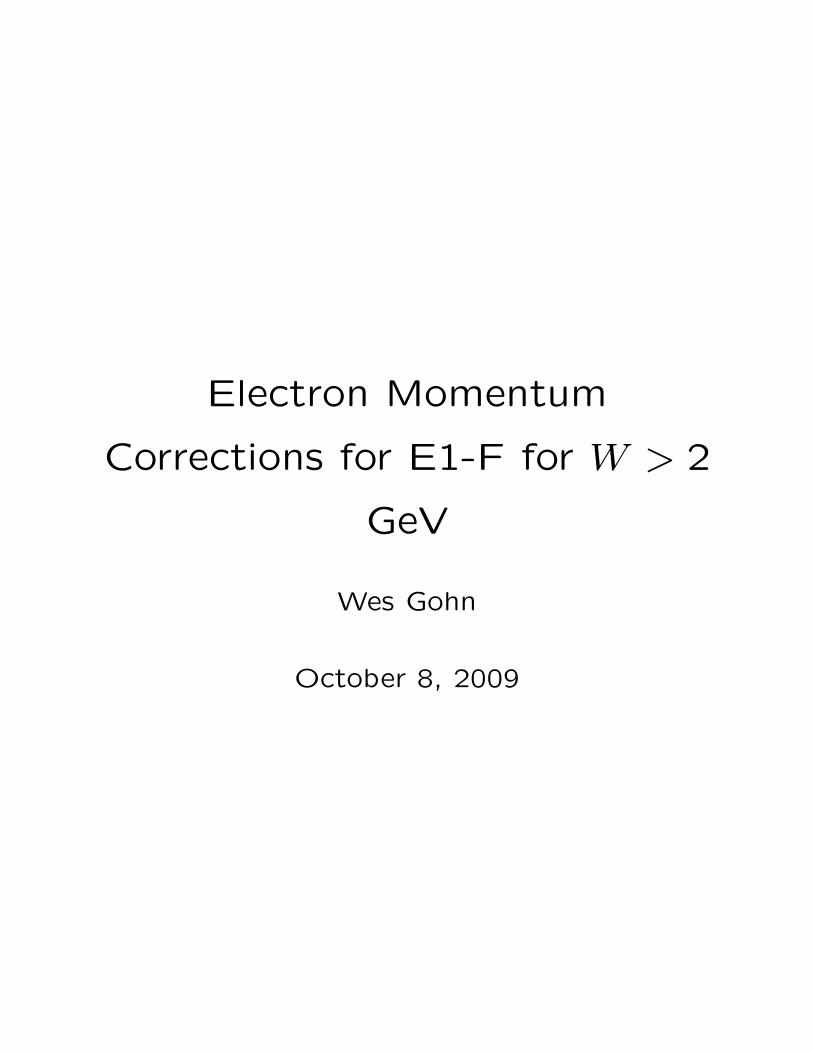
Electron Momentum
Corrections for E1-F for W > 2
GeV
Wes Gohn
October 8, 2009
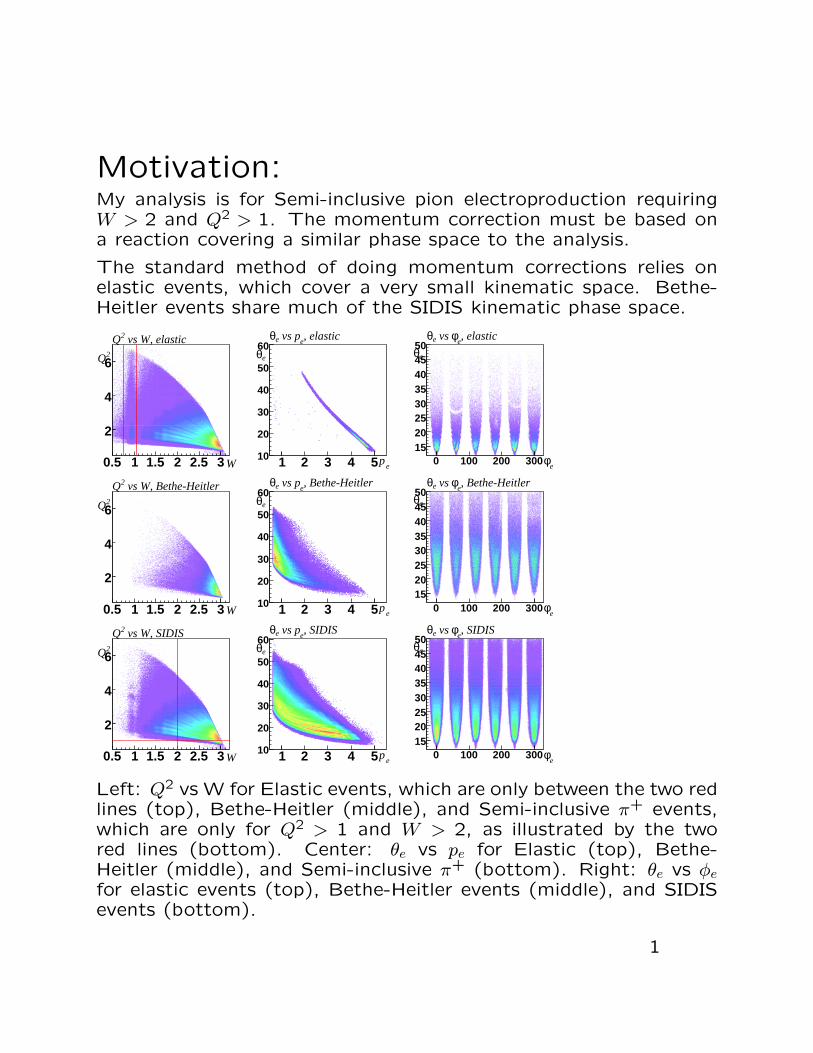
Motivation:My analysis is for Semi-inclusive pion electroproduction requiringW > 2 and Q2 > 1. The momentum correction must be based ona reaction covering a similar phase space to the analysis.
The standard method of doing momentum corrections relies onelastic events, which cover a very small kinematic space. Bethe-Heitler events share much of the SIDIS kinematic phase space.
0.5 1 1.5 2 2.5 3
2
4
62Q
W
vs W, elastic2Q
0.5 1 1.5 2 2.5 3
2
4
62Q
W
vs W, Bethe-Heitler2Q
0.5 1 1.5 2 2.5 3
2
4
62Q
W
vs W, SIDIS2Q
1 2 3 4 510
20
30
40
50
60eθ
ep
, elastice
vs peθ
1 2 3 4 510
20
30
40
50
60eθ
ep
, Bethe-Heitlere
vs peθ
1 2 3 4 510
20
30
40
50
60eθ
ep
, SIDISe
vs peθ
0 100 200 3001520253035404550
eθ
eφ
, elastice
φ vs eθ
0 100 200 3001520253035404550
eθ
eφ
, Bethe-Heitlere
φ vs eθ
0 100 200 3001520253035404550
eθ
eφ
, SIDISe
φ vs eθ
Left: Q2 vs W for Elastic events, which are only between the two redlines (top), Bethe-Heitler (middle), and Semi-inclusive π+ events,which are only for Q2 > 1 and W > 2, as illustrated by the twored lines (bottom). Center: θe vs pe for Elastic (top), Bethe-Heitler (middle), and Semi-inclusive π+ (bottom). Right: θe vs φefor elastic events (top), Bethe-Heitler events (middle), and SIDISevents (bottom).
1

• Momentum correction for electron was performed for W > 2GeV using Bethe-Heitler events.
• An energy loss correction was first applied to the protons usingthe eloss program.
• Bethe-Heitler events identified using a cut on ∆φ < 1.5σ(∆φ = φe − φP) and the point where θγ drops by a factorof e for events passing the previous cut.
• Correction performed in each bin by fitting ∆pp
vs φe with a
linear function.
∆p = pmeasured − pcalc
Pcalc =P ′
1 + P ′(1−cosθe)MP
with
P ′ =MP
1− cosθe(cosθe +
cosθPsinθe
sinθP − 1)
Variable Bin Size Number of Bins RangeW 0.1 GeV 10 2.0GeV < W < 3.0GeVθe 5o 6 15o < θe < 45o
φe 4o 15 −30o < φe < 30o
Binning for Bethe-Heitler events. Binning is performed in eachsector.
2

Testing the technique on elastic events.To test the procedure, we perform the correction for elastic eventsat low W.
Fit with ∆pp
(φ) = A+Bφ+ Cφ2.
-30 -20 -10 0 10 20 30
-0.04
-0.02
0
0.02
0.04
, elastic events, with correction functionφp/p vs ∆pp∆
φ
=2θSector 6, n
-30 -20 -10 0 10 20 30-0.05
-0.04
-0.03
-0.02
-0.01
0
0.01
0.02
0.03
0.04
0.05 , correctedφp/p vs ∆pp∆
φ
0.6 0.7 0.8 0.9 1 1.1 1.20
2000
4000
6000
8000 <20θ15<W, Sector 6
W[GeV]
0.6 0.7 0.8 0.9 1 1.1 1.20
1000
2000
3000
4000
5000<25θ20<
W, Sector 6
W[GeV]
0.6 0.7 0.8 0.9 1 1.1 1.20
500
1000
1500 <30θ25<W, Sector 6
W[GeV]
0.6 0.7 0.8 0.9 1 1.1 1.20
100
200
300
400
500 <35θ30<W, Sector 6
W[GeV]
0.6 0.7 0.8 0.9 1 1.1 1.2020406080
100120
<40θ35<W, Sector 6
W[GeV]
0.6 0.7 0.8 0.9 1 1.1 1.20102030405060 <45θ40<
W, Sector 6
W[GeV]
Uncorrected electron.
Corrected electron
Both plots have the energy loss correction applied for protons.Sector mean W uncorrected σW uncorrected Mean W corrected σW corrected
1 0.974 0.056 0.939 0.0422 0.957 0.052 0.938 0.0453 0.959 0.054 0.938 0.0434 0.955 0.044 0.939 0.0415 0.941 0.046 0.940 0.0406 0.917 0.063 0.939 0.052
3

Bethe-Heitler Event Selection∆φ cut. The example shows each W bin for a single bin in φ andθ.
170 175 180 185 1900
100
200
300
400
500
600
φ∆
Sector 22.0 < W < 2.1
o < 25θ < o20
170 175 180 185 1900100200
300400
500600
700
φ∆
Sector 22.1 < W < 2.2
o < 25θ < o20
170 175 180 185 1900100200300400500600700800900
φ∆
Sector 22.2 < W < 2.3
o < 25θ < o20
170 175 180 185 1900
200
400
600
800
1000
φ∆
Sector 22.3 < W < 2.4
o < 25θ < o20
170 175 180 185 1900
200400
600
800
1000
1200
1400
φ∆
Sector 22.4 < W < 2.5
o < 25θ < o20
170 175 180 185 1900200400600800
10001200140016001800
φ∆
Sector 22.5 < W < 2.6
o < 25θ < o20
170 175 180 185 1900200400600800
100012001400160018002000
φ∆
Sector 22.6 < W < 2.7
o < 25θ < o20
170 175 180 185 1900200400600800
1000120014001600
φ∆
Sector 22.7 < W < 2.8
o < 25θ < o20
170 175 180 185 1900200400600800
1000120014001600180020002200
φ∆
Sector 22.8 < W < 2.9
o < 25θ < o20
170 175 180 185 1900
100
200
300
400
500
600
φ∆
Sector 22.9 < W < 3.0
o < 25θ < o20
∆φ = φe − φp
1.5σ cut around ∆φ peak. The blue histograms illustrate ∆φ pass-ing the θγ cut.
4
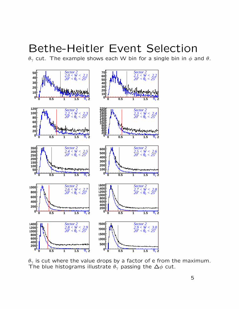
Bethe-Heitler Event Selectionθγ cut. The example shows each W bin for a single bin in φ and θ.
0 0.5 1 1.5 20
10
20
30
40
50
γθ
Sector 22.0 < W < 2.1
o < 25eθ < o20
0 0.5 1 1.5 2010203040506070
γθ
Sector 22.1 < W < 2.2
o < 25eθ < o20
0 0.5 1 1.5 2020406080
100120
γθ
Sector 22.2 < W < 2.3
o < 25eθ < o20
0 0.5 1 1.5 2020406080
100120140160180200220
γθ
Sector 22.3 < W < 2.4
o < 25eθ < o20
0 0.5 1 1.5 2050
100150200250300350
γθ
Sector 22.4 < W < 2.5
o < 25eθ < o20
0 0.5 1 1.5 20100200300400500600
γθ
Sector 22.5 < W < 2.6
o < 25eθ < o20
0 0.5 1 1.5 20
200
400600
800
1000
γθ
Sector 22.6 < W < 2.7
o < 25eθ < o20
0 0.5 1 1.5 20200400600800
1000120014001600
γθ
Sector 22.7 < W < 2.8
o < 25eθ < o20
0 0.5 1 1.5 20200400600800
100012001400
γθ
Sector 22.8 < W < 2.9
o < 25eθ < o20
0 0.5 1 1.5 20
500
1000
1500
2000
2500
γθ
Sector 22.9 < W < 3.0
o < 25eθ < o20
θγ is cut where the value drops by a factor of e from the maximum.The blue histograms illustrate θγ passing the ∆φ cut.
5
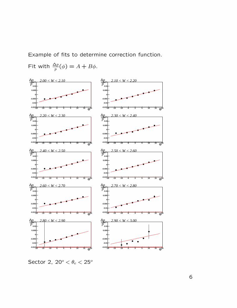
Example of fits to determine correction function.
Fit with ∆pp
(φ) = A+Bφ.
-20 -15 -10 -5 0 5 10 15 20-0.015
-0.01
-0.005
0
0.005
0.01
0.015 2.00 < W < 2.10pp∆
φ -20 -15 -10 -5 0 5 10 15 20-0.015
-0.01
-0.005
0
0.005
0.01
0.015 2.10 < W < 2.20pp∆
φ
-20 -15 -10 -5 0 5 10 15 20-0.015
-0.01
-0.005
0
0.005
0.01
0.015 2.20 < W < 2.30pp∆
φ -20 -15 -10 -5 0 5 10 15 20-0.015
-0.01
-0.005
0
0.005
0.01
0.015 2.30 < W < 2.40pp∆
φ
-20 -15 -10 -5 0 5 10 15 20-0.015
-0.01
-0.005
0
0.005
0.01
0.015 2.40 < W < 2.50pp∆
φ -20 -15 -10 -5 0 5 10 15 20-0.015
-0.01
-0.005
0
0.005
0.01
0.015 2.50 < W < 2.60pp∆
φ
-20 -15 -10 -5 0 5 10 15 20-0.015
-0.01
-0.005
0
0.005
0.01
0.015 2.60 < W < 2.70pp∆
φ -20 -15 -10 -5 0 5 10 15 20-0.015
-0.01
-0.005
0
0.005
0.01
0.015 2.70 < W < 2.80pp∆
φ
-20 -15 -10 -5 0 5 10 15 20-0.015
-0.01
-0.005
0
0.005
0.01
0.015 2.80 < W < 2.90pp∆
φ -20 -15 -10 -5 0 5 10 15 20-0.015
-0.01
-0.005
0
0.005
0.01
0.015 2.90 < W < 3.00pp∆
φ
Sector 2, 20o < θe < 25o
6

Mean of Bethe-Heitler Missing Mass vs. W. Black (circles) showdata with the proton energy loss correction applied, but no mo-mentum correction. Red (squares) show the missing mass afterapplying my correction for electrons. Blue (triangles) show themissing mass after Marco’s correction.
Sector 1.
W [GeV]2 2.2 2.4 2.6 2.8 3
−0.006
−0.004
−0.002
0
0.002
0.004
0.006
vs. W2MMo<20eθ<o15
W [GeV]2 2.2 2.4 2.6 2.8 3
−0.006
−0.004
−0.002
0
0.002
0.004
0.006
vs. W2MMo<25eθ<o20
W [GeV]2 2.2 2.4 2.6 2.8 3
−0.006
−0.004
−0.002
0
0.002
0.004
0.006
vs. W2MMo<30eθ<o25
W [GeV]2 2.2 2.4 2.6 2.8 3
−0.006
−0.004
−0.002
0
0.002
0.004
0.006
vs. W2MMo<35eθ<o30
W [GeV]2 2.2 2.4 2.6 2.8 3
−0.006
−0.004
−0.002
0
0.002
0.004
0.006
vs. W2MMo<40eθ<o35
W [GeV]2 2.2 2.4 2.6 2.8 3
−0.006
−0.004
−0.002
0
0.002
0.004
0.006
vs. W2MMo<45eθ<o40
7

Sector 2.
W [GeV]2 2.2 2.4 2.6 2.8 3
−0.006
−0.004
−0.002
0
0.002
0.004
0.006
vs. W2MMo<20eθ<o15
W [GeV]2 2.2 2.4 2.6 2.8 3
−0.006
−0.004
−0.002
0
0.002
0.004
0.006
vs. W2MMo<25eθ<o20
W [GeV]2 2.2 2.4 2.6 2.8 3
−0.006
−0.004
−0.002
0
0.002
0.004
0.006
vs. W2MMo<30eθ<o25
W [GeV]2 2.2 2.4 2.6 2.8 3
−0.006
−0.004
−0.002
0
0.002
0.004
0.006
vs. W2MMo<35eθ<o30
W [GeV]2 2.2 2.4 2.6 2.8 3
−0.006
−0.004
−0.002
0
0.002
0.004
0.006
vs. W2MMo<40eθ<o35
W [GeV]2 2.2 2.4 2.6 2.8 3
−0.006
−0.004
−0.002
0
0.002
0.004
0.006
vs. W2MMo<45eθ<o40
Sector 3.
W [GeV]2 2.2 2.4 2.6 2.8 3
−0.006
−0.004
−0.002
0
0.002
0.004
0.006
vs. W2MMo<20eθ<o15
W [GeV]2 2.2 2.4 2.6 2.8 3
−0.006
−0.004
−0.002
0
0.002
0.004
0.006
vs. W2MMo<25eθ<o20
W [GeV]2 2.2 2.4 2.6 2.8 3
−0.006
−0.004
−0.002
0
0.002
0.004
0.006
vs. W2MMo<30eθ<o25
W [GeV]2 2.2 2.4 2.6 2.8 3
−0.006
−0.004
−0.002
0
0.002
0.004
0.006
vs. W2MMo<35eθ<o30
W [GeV]2 2.2 2.4 2.6 2.8 3
−0.006
−0.004
−0.002
0
0.002
0.004
0.006
vs. W2MMo<40eθ<o35
W [GeV]2 2.2 2.4 2.6 2.8 3
−0.006
−0.004
−0.002
0
0.002
0.004
0.006
vs. W2MMo<45eθ<o40
8

Sector 4.
W [GeV]2 2.2 2.4 2.6 2.8 3
−0.006
−0.004
−0.002
0
0.002
0.004
0.006
vs. W2MMo<20eθ<o15
W [GeV]2 2.2 2.4 2.6 2.8 3
−0.006
−0.004
−0.002
0
0.002
0.004
0.006
vs. W2MMo<25eθ<o20
W [GeV]2 2.2 2.4 2.6 2.8 3
−0.006
−0.004
−0.002
0
0.002
0.004
0.006
vs. W2MMo<30eθ<o25
W [GeV]2 2.2 2.4 2.6 2.8 3
−0.006
−0.004
−0.002
0
0.002
0.004
0.006
vs. W2MMo<35eθ<o30
W [GeV]2 2.2 2.4 2.6 2.8 3
−0.006
−0.004
−0.002
0
0.002
0.004
0.006
vs. W2MMo<40eθ<o35
W [GeV]2 2.2 2.4 2.6 2.8 3
−0.006
−0.004
−0.002
0
0.002
0.004
0.006
vs. W2MMo<45eθ<o40
Sector 5.
W [GeV]2 2.2 2.4 2.6 2.8 3
−0.006
−0.004
−0.002
0
0.002
0.004
0.006
vs. W2MMo<20eθ<o15
W [GeV]2 2.2 2.4 2.6 2.8 3
−0.006
−0.004
−0.002
0
0.002
0.004
0.006
vs. W2MMo<25eθ<o20
W [GeV]2 2.2 2.4 2.6 2.8 3
−0.006
−0.004
−0.002
0
0.002
0.004
0.006
vs. W2MMo<30eθ<o25
W [GeV]2 2.2 2.4 2.6 2.8 3
−0.006
−0.004
−0.002
0
0.002
0.004
0.006
vs. W2MMo<35eθ<o30
W [GeV]2 2.2 2.4 2.6 2.8 3
−0.006
−0.004
−0.002
0
0.002
0.004
0.006
vs. W2MMo<40eθ<o35
W [GeV]2 2.2 2.4 2.6 2.8 3
−0.006
−0.004
−0.002
0
0.002
0.004
0.006
vs. W2MMo<45eθ<o40
9

Sector 6.
W [GeV]2 2.2 2.4 2.6 2.8 3
−0.006
−0.004
−0.002
0
0.002
0.004
0.006
vs. W2MMo<20eθ<o15
W [GeV]2 2.2 2.4 2.6 2.8 3
−0.006
−0.004
−0.002
0
0.002
0.004
0.006
vs. W2MMo<25eθ<o20
W [GeV]2 2.2 2.4 2.6 2.8 3
−0.006
−0.004
−0.002
0
0.002
0.004
0.006
vs. W2MMo<30eθ<o25
W [GeV]2 2.2 2.4 2.6 2.8 3
−0.006
−0.004
−0.002
0
0.002
0.004
0.006
vs. W2MMo<35eθ<o30
W [GeV]2 2.2 2.4 2.6 2.8 3
−0.006
−0.004
−0.002
0
0.002
0.004
0.006
vs. W2MMo<40eθ<o35
W [GeV]2 2.2 2.4 2.6 2.8 3
−0.006
−0.004
−0.002
0
0.002
0.004
0.006
vs. W2MMo<45eθ<o40
Sector Mean, No Correction σ, No Correction Mean, My Correction σ, My Correction Mean, Marco’s Correction σ, Marco’s Correction1 0.0022 0.0199 -0.0006 0.0194 -0.0018 0.01942 0.0022 0.0196 0.0002 0.0191 -0.0006 0.01923 0.0016 0.0198 -0.0010 0.0196 -0.0018 0.01994 0.0018 0.0198 -0.0005 0.0195 -0.0032 0.01975 -0.0004 0.0197 -0.0007 0.0195 -0.0034 0.01956 -0.0013 0.0199 -0.0007 0.0198 -0.0010 0.0197
10

Missing Mass from ep→ eπ+XThe top set of plots show data with no electron momentum correc-tion, and the bottom six plots show data with my electron momen-tum correction applied. Both sets have the energy loss correctionapplied for π+.
Entries 1291159
0.6 0.7 0.8 0.9 1 1.1 1.20
2000
4000
6000
8000
10000
12000
Entries 1291159
mean = 0.947
= 0.027σ
sector 1
Missing Mass [GeV]
, uncorrectedXM Entries 985941
0.6 0.7 0.8 0.9 1 1.1 1.20
2000
4000
6000
8000
10000
12000
Entries 985941
mean = 0.944
= 0.023σ
sector 2
Missing Mass [GeV]
, uncorrectedXM Entries 1069238
0.6 0.7 0.8 0.9 1 1.1 1.20
2000
4000
6000
8000
10000
Entries 1069238
mean = 0.940
= 0.025σ
sector 3
Missing Mass [GeV]
, uncorrectedXM
Entries 929193
0.6 0.7 0.8 0.9 1 1.1 1.20
2000
4000
6000
8000
10000
12000
Entries 929193
mean = 0.952
= 0.023σ
sector 4
Missing Mass [GeV]
, uncorrectedXM Entries 1013756
0.6 0.7 0.8 0.9 1 1.1 1.20
5000
10000
15000
Entries 1013756
mean = 0.939
= 0.023σ
sector 5
Missing Mass [GeV]
, uncorrectedXM Entries 990350
0.6 0.7 0.8 0.9 1 1.1 1.20
2000
4000
6000
8000
10000
Entries 990350
mean = 0.925
= 0.032σ
sector 6
Missing Mass [GeV]
, uncorrectedXM
Entries 1291159
0.6 0.7 0.8 0.9 1 1.1 1.20
5000
10000
15000
Entries 1291159
mean = 0.946
= 0.023σ
sector 1
Missing Mass [GeV]
, correctedXM Entries 985941
0.6 0.7 0.8 0.9 1 1.1 1.20
2000
4000
6000
8000
10000
12000
Entries 985941
mean = 0.940
= 0.022σ
sector 2
Missing Mass [GeV]
, correctedXM Entries 1069238
0.6 0.7 0.8 0.9 1 1.1 1.20
2000
4000
6000
8000
10000
12000
Entries 1069238
mean = 0.940
= 0.024σ
sector 3
Missing Mass [GeV]
, correctedXM
Entries 929193
0.6 0.7 0.8 0.9 1 1.1 1.20
2000
4000
6000
8000
10000
12000
Entries 929193
mean = 0.950
= 0.023σ
sector 4
Missing Mass [GeV]
, correctedXM Entries 1013756
0.6 0.7 0.8 0.9 1 1.1 1.20
5000
10000
15000
Entries 1013756
mean = 0.940
= 0.022σ
sector 5
Missing Mass [GeV]
, correctedXM Entries 990350
0.6 0.7 0.8 0.9 1 1.1 1.20
2000
4000
6000
8000
10000
Entries 990350
mean = 0.925
= 0.032σ
sector 6
Missing Mass [GeV]
, correctedXM
Sector 1 2 3 4 5 6Uncorrected Mean 0.947 0.944 0.940 0.952 0.939 0.925
Corrected Mean 0.946 0.940 0.940 0.950 0.940 0.925Uncorrected σ 0.027 0.023 0.025 0.023 0.023 0.032
Corrected σ 0.023 0.022 0.024 0.023 0.022 0.032
11

Conclusion:Below are histograms showing distributions of W and Q2. Theblack histogram shows each distribution without electron momen-tum correction, and the red line draws the histogram after theelectron momentum correction.
W [GeV]1 1.5 2 2.5 30
5000
10000
15000
20000
25000
30000
35000
40000
45000
X+π e→W, ep
]2 [GeV2Q1 2 3 4 50
10000
20000
30000
40000
50000
60000
70000
X+π e→, ep2Q
• Electron momentum corrections have been performed individ-ually in each bin
• While in many bins they are comparable to Marco’s correction,there are some bins in which this correction gives us Bethe-Heitler missing mass results considerably closer to zero.
• The semi-inclusive missing mass, Q2, and W spectra are notstrongly affected by the correction.
12

Support Slides
13

Missing Mass Fits
-0.1 -0.05 0 0.05 0.10102030405060708090
2θ, Sector 4, n2XBH M
2.00 < W < 2.10=0.014395σ=-0.000314, µ=0.014220σ=-0.000463, µ=0.014249σ=-0.003042, µ
-0.1 -0.05 0 0.05 0.10102030405060708090
2θ, Sector 4, n2XBH M
2.10 < W < 2.20=0.016056σ=-0.000767, µ=0.016056σ=-0.000767, µ=0.015909σ=-0.003669, µ
-0.1 -0.05 0 0.05 0.1020406080
100120140
2θ, Sector 4, n2XBH M
2.20 < W < 2.30=0.017150σ=0.000073, µ=0.017150σ=0.000073, µ=0.017078σ=-0.002982, µ
-0.1 -0.05 0 0.05 0.1020406080
100120140160
2θ, Sector 4, n2XBH M
2.30 < W < 2.40=0.016862σ=0.000619, µ=0.016696σ=-0.000273, µ=0.016834σ=-0.002572, µ
-0.1 -0.05 0 0.05 0.10
50
100
150
200
250 2θ, Sector 4, n2
XBH M
2.40 < W < 2.50=0.017374σ=0.001222, µ=0.017182σ=0.000346, µ=0.017292σ=-0.002070, µ
-0.1 -0.05 0 0.05 0.1050
100150200250300
2θ, Sector 4, n2XBH M
2.50 < W < 2.60=0.017902σ=0.001672, µ=0.017710σ=-0.000629, µ=0.017845σ=-0.001805, µ
-0.1 -0.05 0 0.05 0.1050
100150200250300350400450
2θ, Sector 4, n2XBH M
2.60 < W < 2.70=0.018387σ=0.002532, µ=0.018323σ=-0.000182, µ=0.018339σ=-0.001274, µ
-0.1 -0.05 0 0.05 0.10100200300400500600
2θ, Sector 4, n2XBH M
2.70 < W < 2.80=0.019437σ=0.002907, µ=0.019387σ=-0.000123, µ=0.019434σ=-0.001421, µ
-0.1 -0.05 0 0.05 0.1050
100150200250300350400450
2θ, Sector 4, n2XBH M
2.80 < W < 2.90=0.021281σ=0.003418, µ=0.021266σ=-0.000374, µ=0.021250σ=-0.001996, µ
-0.1 -0.05 0 0.05 0.1020406080
100120140
2θ, Sector 4, n2XBH M
2.90 < W < 3.00=0.023690σ=0.005150, µ=0.023872σ=-0.000813, µ=0.024004σ=-0.002011, µ
14