electron probe microanalysis: principles and...

MT.4

Electron probe microanalysis: principles

and applications

Xavier Llovet

Unitat Microsonda Electrònica, CCiTUB, Universitat de Barcelona. Lluís Solé i Sabarís, 1-3. 08028 Barcelona. Spain.

email: [email protected]

Abstract. This article summarizes the basic principles of electron probe microanalysis, with examples of applications in materials science and geology

that illustrate the capabilities of the technique.

Handbook of instrumental techniques from CCiTUB

Electron probe microanalysis

1

MT.4

IntroductionIntroductionIntroductionIntroduction

Electron probe microanalysis (EPMA) is a nondestructive analytical technique widely used for determining the local composition of solid samples [1, 2, 3]. The technique is based on the measurement of characteristic x-ray intensities emitted by the elements present in the sample when the latter is bombarded with a focused electron beam. For each element, the ratio of the characteristic x-ray intensity emitted from the sample to that emitted from a standard of known composition is measured. This ratio is usually referred to as k-ratio. The transformation from measured k-ratios to concentrations is performed by means of relatively simple, analytical algorithms, which assume that the sample region from which x rays emerge has a homogeneous composition. For keV electron beams, this region is typically about 1 µm, depending on the density of the material and the analytical conditions. Accordingly, EPMA is suitable for the analysis of samples that are homogeneous on the micron scale.

Using wavelength-dispersive (WD) spectrometers, elements from Be to U can be analyzed by EPMA with detection limits for most elements down to 100 ppm or lower, accuracy of 2% for major element concentrations and a spatial resolution of few microns. EPMA also couples quantitative analytical capabilities with the imaging capabilities of a scanning electron microscope (SEM), allowing detailed x-ray mapping of composition contrast. Moreover, EPMA can also be used to determine the thickness and composition of thin films and multilayers with thickness in the sub-micron range, providing information on the lateral variation in thickness and composition at the micrometer scale. EPMA is extensively used in many fields and has been central for the microanalysis of ceramic, metallurgical, geological, biological, and other materials.

The first electron microprobe was developed by Raimond Castaing in 1950 by fitting a crystal spectrometer to a modified electron microscope. Using the developed instrument, Castaing established the basic principles of quantitative EPMA [4]. A few years later, in 1958, the French company CAMECA manufactured the first commercial electron microprobe. Since then, many improvements in the probe-forming system, as well as in the x-ray spectrometers have been performed, which have advanced electron microprobes, in terms of stability, reproducibility and detection limits. Recently, the incorporation of field-emission electron sources in EPMA equipment has opened the possibility of obtaining x-ray maps of chemical contrast and point analyses with sub-micron spatial resolution.

This article summarizes the basic principles of EPMA, with examples of applications that illustrate the capabilities of the technique.

1. 1. 1. 1. MethodologyMethodologyMethodologyMethodology

1.1. Physical principles When an electron beam impinges on a sample, electrons interact repeatedly with the sample atoms until they come to rest or emerge from the surface. In the keV energy range, the possible interactions of electrons with atoms are elastic scattering, inelastic collisions and bremsstrahlung emission [5, 6]. Elastic interactions are those in which the initial and final states of the atom are the same, normally the ground state. These interactions change the direction of movement of the electrons. Inelastic collisions are those in which the atom is brought to an excited state, i.e. a part of the electron’s kinetic energy is taken up by the atomic electrons. Inelastic collisions include excitation of electrons in the conduction or valence bands, plasmon excitations and inner-shell ionization, i.e. the production of a vacancy in an inner-electron shell (see Fig. 1). After inner-shell ionization, the atom de-excites by migration of the vacancy to outer shells through a cascade of electron transitions and energy is released as characteristic x rays or Auger electrons. Inner-shell ionization is thus responsible for the emission of characteristic x rays. Emission of bremsstrahlung takes place when the electron is decelerated in the electrostatic field of the target atom. Bremsstrahlung emission has almost no effect on the electron trajectories but it is the source of the continuous background in an x-ray spectrum.


2

MT.4

Emitted photons (either as characteristic x rays or bremsstrahlung) originate at sample depths extending from the surface to some maximum depth, which depends on the material and on the energy of incident electrons. Before emerging from the surface, generated x rays may interact with the sample atoms through different mechanisms, mainly photoelectric absorption, and as a result, fluorescent x rays may be emitted.

Figure 1. Schematic diagram of the different atomic inner atomic shells and main possible transitions to these shells that release characteristic x rays.

1.2. Instrumentation The electron microprobe essentially consists of an electron column and several x-ray spectrometers, which can be WD and/or energy-dispersive (ED) spectrometers.

The electron column consists of an electron gun and an electromagnetic lens system (see Fig.2). The electron gun acts as a source of electrons. It is commonly a thermoionic gun, usually made of W or LaB6 which is heated to liberate electrons by thermionic emission. The filament is held at a negative potential by a power supply, which accelerates the electrons escaping from the filament through an aperture. Typical accelerating voltages range from 1 kV up to 40 kV. The electromagnetic lenses are used to focus the electron beam onto the target, with a final diameter of about 0.1-1 µm. They are also used to control the electron current, i.e. the number of incoming electrons per unit time, with values typically of 1-300 nA. The electron current is measured with a Faraday cup and stabilized by means of a beam regulator device. The sample is connected to ground to ensure electron conductivity.

Conventional high vacuum technology is generally used in order to prevent oxidation of the filament, breakdown of the accelerating voltage and scattering of the electrons in the beam by the residual gas. In order to minimize carbon contamination at the point of electron impact due to the cracking of hydrocarbons present in the chamber, the electron microprobe is equipped with a liquid nitrogen “cold finger”, placed close to the specimen, and an air jet directed towards the point of electron impact.

An optical microscope co-axial to the electron beam is commonly used to locate the areas of interest in the sample. For the same purpose, the beam can be scanned as in conventional SEMs. Images can then be generated by using the signal from an electron detector, which usually records secondary (SE) and/or backscattered electrons (BSE) from the target.

The WD spectrometer consists of a crystal monochromator and an x-ray detector, usually a gas proportional counter, arranged in such a way that x rays impinging on the crystal are diffracted according to Bragg’s law and some of them reach the detector and are recorded. The Bragg law reads n λ=2 d sinθ, where λ is the x ray wavelength, n is the diffraction order, d is the spacing between atomic planes of the monochromator crystal and θ is the angle of incidence of the x rays.

With flat crystals and point x-ray sources, Bragg reflection occurs only on a small portion of the crystal surface. Improved reflection is obtained by placing the target, the crystal and the detector on a focal circle of radius R (the Rowland circle) and bending the atomic planes of the crystal to a radius 2R. This focussing geometry is known as the “Johann” type. Much improved reflection is obtained if the crystal surface is bent to the radius R (“Johansson” type). With this arrangement, the


3

MT.4

angle of incidence of x rays is constant over the line defined by the intersection of the Rowland circle plane and the crystal surface. Coordinated mechanical rotation of the crystal and the detector allows us to record the x-ray spectrum as a function of wavelength. In the focussing geometries, the source-crystal distance is proportional to sinθ and thus proportional to the wavelength. Therefore, the crystal is simultaneously rotated and moved along a straight line by means of mechanical linkage. This allows calibration of the wavelength by just measuring the source-crystal distance and moreover, the take-off angle is kept constant for all wavelengths.

Figure 2: Cross section of an electron microprobe.

Figure 3: Electron microprobe CAMECA SX-50 at the CCiTUB (4 WD spectrometers + 1 EDS).

Besides mechanical limitations of the crystal driver, the range of reflected wavelengths is only

limited by the crystal inter-atomic spacing d and, therefore, crystals with different spacings are required to cover a wide wavelength range. Crystals commonly used for microanalysis are Lithium Fluoride (LiF), Pentaerythritol (PET), and Thallium Acid Phthalate (TAP). The wavelength range covered by using these three crystals is λ ∼ 1-24 Å. For longer wavelengths, layered synthetic multistructures (LSM) consisting of many alternating layers of high- and low-Z materials, such as W/Si, Ni/C and Mo/BC can be employed. In these cases, d is equal to the sum of the thickness of one layer pair of the high-Z and low-Z materials.

The gas proportional counter consists of a gas-filled tube with a coaxial wire held at a potential of 1-2 kV with respect to the outer wall of the tube. X rays enter the counter through a window; they are absorbed by the gas molecules through photoelectric effect and generate free photoelectrons, which are accelerated by the electric field and produce a cascade of secondary electrons. As a result, each incoming x ray produces a pulse whose height is proportional to the energy of the x ray. The output pulses are sent to a pulse-height analyzer (PHA) that counts pulses with selected heights –usually contained within a certain voltage window–. Visualization of the PHA display helps us to properly select the values of the counter high voltage, the gain and the discriminatory settings (baseline and window). Proportional counters can be of flow type, in which case the gas escapes through the window and therefore must be supplied continuously, or of the sealed type. Since WD spectrometers only allow the recording of one wavelength at a time, electron microprobes are usually equipped with several (up to 5) spectrometers (Fig. 3), each with several interchangeable crystals.

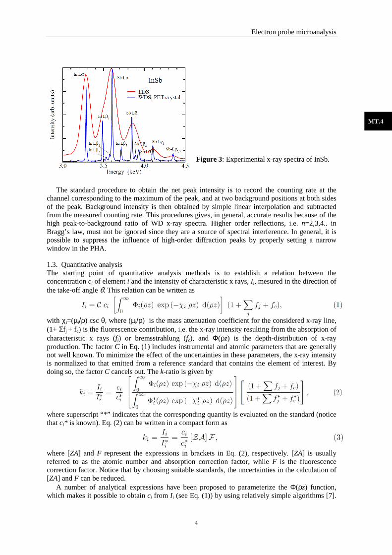
The ED spectrometer uses a solid-state x-ray detector, usually a crystal semiconductor such as Si or Ge, which discriminates x rays based on their energy. In Fig. 3, x-ray spectra of InSb recorded with WD and ED spectrometers are compared. In the ED spectrum, the overlap between adjacent lines makes it difficult to obtain the corresponding x-ray intensities, while for the WD spectrum, the majority of x-ray lines are clearly resolved. Because of its better resolution, WD spectrometers have better (lower) detection limits than ED spectrometers (typically ten times).


4

MT.4

Figure 3: Experimental x-ray spectra of InSb.

The standard procedure to obtain the net peak intensity is to record the counting rate at the

channel corresponding to the maximum of the peak, and at two background positions at both sides of the peak. Background intensity is then obtained by simple linear interpolation and subtracted from the measured counting rate. This procedures gives, in general, accurate results because of the high peak-to-background ratio of WD x-ray spectra. Higher order reflections, i.e. n=2,3,4.. in Bragg’s law, must not be ignored since they are a source of spectral interference. In general, it is possible to suppress the influence of high-order diffraction peaks by properly setting a narrow window in the PHA.

1.3. Quantitative analysis The starting point of quantitative analysis methods is to establish a relation between the concentration ci of element i and the intensity of characteristic x rays, Ii, mesured in the direction of the take-off angle θ. This relation can be written as

with χi=(µi/ρ) csc θ, where (µi/ρ) is the mass attenuation coefficient for the considered x-ray line, (1+ Σf j + fc) is the fluorescence contribution, i.e. the x-ray intensity resulting from the absorption of characteristic x rays (fi) or bremsstrahlung (fc), and Φ(ρz) is the depth-distribution of x-ray production. The factor C in Eq. (1) includes instrumental and atomic parameters that are generally not well known. To minimize the effect of the uncertainties in these parameters, the x-ray intensity is normalized to that emitted from a reference standard that contains the element of interest. By doing so, the factor C cancels out. The k-ratio is given by

where superscript “*” indicates that the corresponding quantity is evaluated on the standard (notice that ci* is known). Eq. (2) can be written in a compact form as

where [ZA] and F represent the expressions in brackets in Eq. (2), respectively. [ZA] is usually referred to as the atomic number and absorption correction factor, while F is the fluorescence correction factor. Notice that by choosing suitable standards, the uncertainties in the calculation of [ZA] and F can be reduced.

A number of analytical expressions have been proposed to parameterize the Φ(ρz) function, which makes it possible to obtain ci from Ii (see Eq. (1)) by using relatively simple algorithms [7].


5

MT.4

Examples of such parameterizations are the widely used PAP [8] or X-PHI [9] models. In practice, k-ratios are measured for all elements present in the sample (except for those estimated by stoichiometry or by other means) and the resulting system of equations is solved by using an iterative procedure. This is so because the factors [ZA] and F that occur in Eq. (3) depend themselves on sample composition. In general, convergence is quickly achieved using simple iterative procedures.

As mentioned in the introduction, EPMA can also be used to determine the thickness and composition of thin films and multilayers. Correction procedures that allow the analysis of thin films and multilayers are known as thin-film programs [10]. Examples of available thin-film programs are the widely used STRATAGEM [11] or X-FILM [12]. For the analysis of heterogeneous samples such as sub-micron particles, embedded inclusions or lamellae structures, the simplifications underlying correction procedures are not firmly established and there is a need for more realistic procedures. In this context, the Monte Carlo simulation method [13] is a valuable tool as a basis of quantitative procedures.

2. 2. 2. 2. Examples of applicationsExamples of applicationsExamples of applicationsExamples of applications

EPMA capabilities include point analysis, line profiles and x-ray mappings, both qualitative and quantitative, as well as the determination of the composition and thickness of thin films and multilayers. Applications of EPMA in the earth and environmental sciences include the description and classification of rocks (mineral chemistry); identification of minerals; determination of temperatures and pressures of rock formation (geothermobarometry); chemical zoning within mineral crystals on the micron-scale for petrological, crystal growth and diffusion studies (e.g. for the determination of time scales of magmatic and volcanic processes); study of mineral indicators in mineral exploration; analysis of minerals of economic and strategic importance (e.g. ore deposits, carbon sequestration); study of fossil materials, limestones and corals; determination of rock ages via U-Pb radioactive decays.

In materials science and physical metallurgy, EPMA is extensively used for the determination of the chemical composition and microstructure of alloys, steel, metals, glass, ceramics, composite and advanced materials; determination of phase diagrams; analysis of inclusions and precipitates; analysis of elemental distributions, e.g. diffusion profiles, depletion zones, nitrided and carburized surfaces, corrosion and oxidation phenomena; analysis of thin films and coatings.

EPMA can also be used as a scattering chamber to determine physical quantities related to the production of x rays (e.g. [14]) which are needed in medical and industrial applications.

In this section, we show some of our own examples of applications of EPMA which briefly illustrate the capabilities of the technique.

2.1. Characterization of duplex stainless steel Duplex stainless steels (DSS) are a family of steel grades that have a two-phase microstructure consisting of grains of ferritic (α) and austenitic (γ) stainless steel, with diameters of several micrometers. These steels are valuable for applications where good mechanical and anti-corrosion properties are required simultaneously, such as refinery pipes or off-shore platforms. The use of DSS at high temperatures requires knowledge of the phase transformations that they undergo after heat treatment. The most important phases that occur during heat treatment are the so-called σ and χ phases, which form between 650 oC and 1000 oC mainly at the α/γ interface, and are associated with a reduction of anticorrosion and toughness properties. Other phases that can occur in the same range of temperatures are secondary austenite (γ2), and several nitrides and carbides. EPMA is a valuable tool for the characterization of DSS as it combines micrometer spatial resolution with low detection limits.

Figure 3 shows the microstructure of a DSS sample after heat treatment (8h, 850oC) [15]. The following phases can be observed: ferrite (α), austenite (γ), secondary austenite (γ2), and the σ and χ phases. Figure 4 displays a portion of the x-ray spectrum near the N Kα line emitted from an austenite grain. Nitrogen plays an important role on the properties of DSS as it can partially replace


6

MT.4

Ni, which is of economic interest. Accurate measurement of N is difficult mainly because of its low peak-to-background ratio and the curved background under the peak (see Fig. 4). One way of overcoming this difficulty is to use a calibration curve, which can be obtained from (mono-phase) steel reference samples [16]. Typical EPMA analyses of the observed phases are shown in Table 1. In this example, the detection limit (DL) of N is ∼ 0.025 wt.%; the precision of the N determination is ∼ 15-20 % for the α and σ phases and ∼ 5% for the γ and χ phases [15].

Figure 3: BSE image showing the microstructure of a DSS after heat

treatment.

Figure 4: X-ray spectra around the position of N measured on an austenite grain (γ).

Table 1: Phase composition of a duplex stainless steel after heat treatment (8h, 850 oC)

Phase type wt.% Austenite (γ) Sec. aust. (γ2) Ferrite (α) Phase σ Phase χ N 0.40 <DL 0.05 0.07 0.14 Si 0.21 0.56 0.25 0.38 0.38 Cr 20.28 18.39 22.84 27.65 23.27 Mn 4.48 4.73 3.47 4.25 4.56 Fe 68.81 69.96 68.97 59.01 58.61 Ni 2.97 3.25 1.47 1.40 1.22 Cu 1.14 1.29 0.73 0.31 0.27 Mo 2.30 1.81 2.71 7.92 15.01 Total 100. 59 99.99 100.49 101.09 103.46

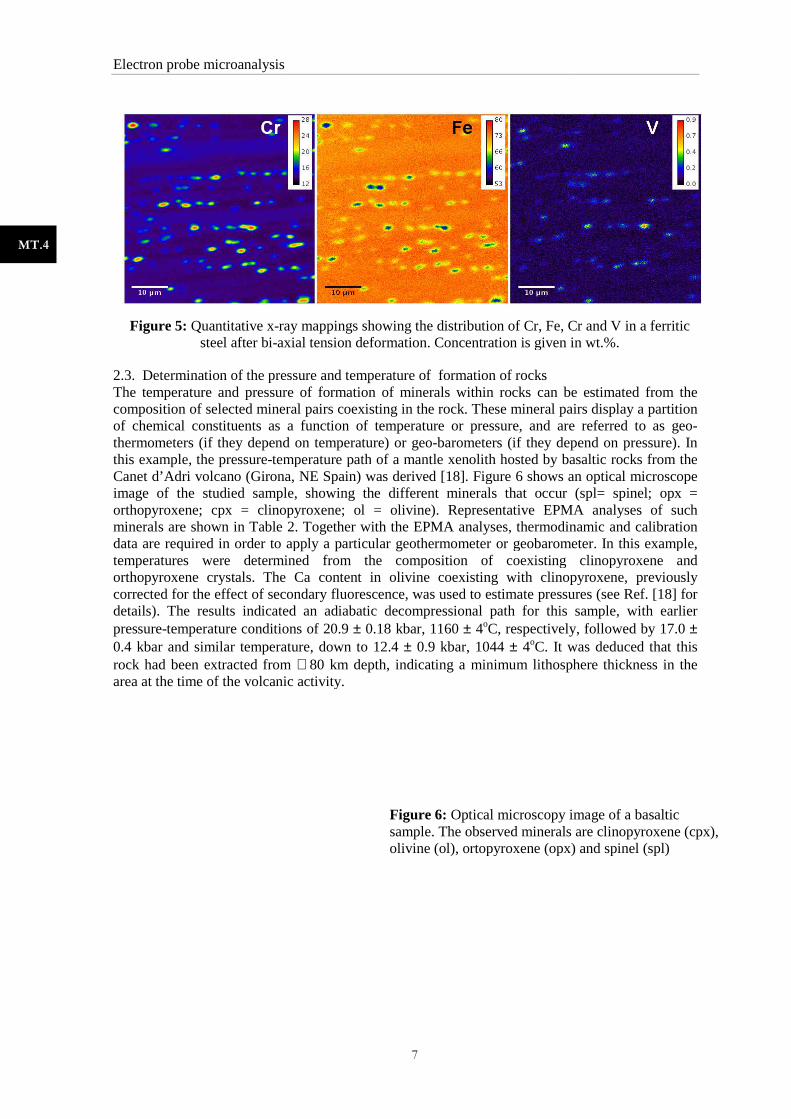
2.2. Analysis of chemical segregation in ferritic steel Applications of ferritic stainless steels are commonly related to conformation, usually stretching and deep drawing, of house-hold appliances. These applications require knowledge of the deformation mechanisms of these steels and the effect of microstructure and microsegregation on their behaviour during deformation. A convenient method to analyze microsegregation is by means of x-ray mapping, which allows to record the distribution of elements over an area of the sample. Depending on the area, x-ray mappings can be obtained by scanning the beam across the sample or, alternatively, by moving the sample back and forth under a fixed electron beam. Mappings can display x-ray intensity in each pixel (qualitative) or concentration (quantitative). The mappings of Fig. 5 show the quantitative distribution of Fe, Cr and V in ferritic stainless steel after bi-axial tension deformation [17]. The colormap at the righ-hand side of each map displays the equivalence between color and concentration (in wt. %). In this example, x-ray mapping allowed to correlate the effect of tension deformation with the intensity and width of microsegregation [17].


MT.4

Figure 5: Quantitative x-ray steel after bi-axial tension

2.3. Determination of the pressure and The temperature and pressure composition of selected mineral pairs of chemical constituents as a function of temperature or pressure, and are referred to as geothermometers (if they depend on temperature) or geothis example, the pressure-temperature pathCanet d’Adri volcano (Girona, NE Spain) image of the studied sample, showing the different minerals thatorthopyroxene; cpx = clinopyroxene; ol = olivine). Representative EPMA analyses of such minerals are shown in Table data are required in order to aptemperatures were determined from the composition of coexisting clinopyroorthopyroxene crystals. The corrected for the effect of secdetails). The results indicated an adiabatic decompressional path for this sample, with earlier pressure-temperature conditions of 20.9 0.4 kbar and similar temperature, rock had been extracted from area at the time of the volcanic activity.

7

ray mappings showing the distribution of Cr, Fe, Cr and V in a ferritic axial tension deformation. Concentration is given in wt.%

Determination of the pressure and temperature of formation of rocks The temperature and pressure of formation of minerals within rocks can be estimated from the

selected mineral pairs coexisting in the rock. These mineral pairs display a partition of chemical constituents as a function of temperature or pressure, and are referred to as geothermometers (if they depend on temperature) or geo-barometers (if they depend on pressure).

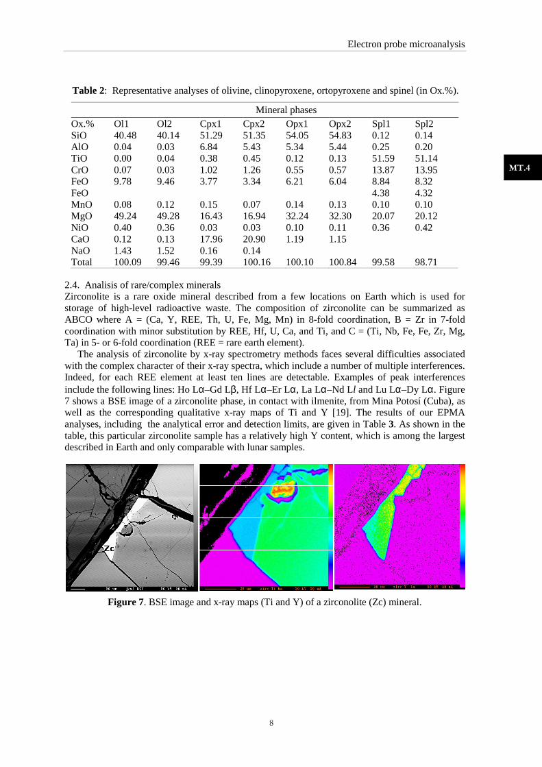
temperature path of a mantle xenolith hosted by basaltic rockCanet d’Adri volcano (Girona, NE Spain) was derived [18]. Figure 6 shows an optical microscop

sample, showing the different minerals that occur (spl= spinel; opx = orthopyroxene; cpx = clinopyroxene; ol = olivine). Representative EPMA analyses of such minerals are shown in Table 2. Together with the EPMA analyses, thermodinamic and calibration

required in order to apply a particular geothermometer or geobarometer. In this example, temperatures were determined from the composition of coexisting clinopyro

Ca content in olivine coexisting with clinopyroxene,fect of secondary fluorescence, was used to estimate pressures (see

esults indicated an adiabatic decompressional path for this sample, with earlier temperature conditions of 20.9 ± 0.18 kbar, 1160 ± 4oC, respectively, followed b

0.4 kbar and similar temperature, down to 12.4 ± 0.9 kbar, 1044 ± 4oC. It was deduced that this rock had been extracted from ∼ 80 km depth, indicating a minimum lithosphere thickness in the area at the time of the volcanic activity.

Figure 6: Optical microscopy image of a basaltic sample. The observed minerals are clinopyroxene (cpx), olivine (ol), ortopyroxene (opx) and spinel (spl)

Cr and V in a ferritic Concentration is given in wt.%.

can be estimated from the coexisting in the rock. These mineral pairs display a partition

of chemical constituents as a function of temperature or pressure, and are referred to as geo-barometers (if they depend on pressure). In

basaltic rocks from the was derived [18]. Figure 6 shows an optical microscope

occur (spl= spinel; opx = orthopyroxene; cpx = clinopyroxene; ol = olivine). Representative EPMA analyses of such

odinamic and calibration or geobarometer. In this example,

temperatures were determined from the composition of coexisting clinopyroxene and coexisting with clinopyroxene, previously

was used to estimate pressures (see Ref. [18] for esults indicated an adiabatic decompressional path for this sample, with earlier

C, respectively, followed by 17.0 ± C. It was deduced that this

80 km depth, indicating a minimum lithosphere thickness in the

Optical microscopy image of a basaltic sample. The observed minerals are clinopyroxene (cpx), olivine (ol), ortopyroxene (opx) and spinel (spl)


8

MT.4

Table 2: Representative analyses of olivine, clinopyroxene, ortopyroxene and spinel (in Ox.%).

Mineral phases Ox.% Ol1 Ol2 Cpx1 Cpx2 Opx1 Opx2 Spl1 Spl2 SiO 40.48 40.14 51.29 51.35 54.05 54.83 0.12 0.14 AlO 0.04 0.03 6.84 5.43 5.34 5.44 0.25 0.20 TiO 0.00 0.04 0.38 0.45 0.12 0.13 51.59 51.14 CrO 0.07 0.03 1.02 1.26 0.55 0.57 13.87 13.95 FeO 9.78 9.46 3.77 3.34 6.21 6.04 8.84 8.32 FeO 4.38 4.32 MnO 0.08 0.12 0.15 0.07 0.14 0.13 0.10 0.10 MgO 49.24 49.28 16.43 16.94 32.24 32.30 20.07 20.12 NiO 0.40 0.36 0.03 0.03 0.10 0.11 0.36 0.42 CaO 0.12 0.13 17.96 20.90 1.19 1.15 NaO 1.43 1.52 0.16 0.14 Total 100.09 99.46 99.39 100.16 100.10 100.84 99.58 98.71

2.4. Analisis of rare/complex minerals Zirconolite is a rare oxide mineral described from a few locations on Earth which is used for storage of high-level radioactive waste. The composition of zirconolite can be summarized as ABCO where A = (Ca, Y, REE, Th, U, Fe, Mg, Mn) in 8-fold coordination, B = Zr in 7-fold coordination with minor substitution by REE, Hf, U, Ca, and Ti, and C = (Ti, Nb, Fe, Fe, Zr, Mg, Ta) in 5- or 6-fold coordination (REE = rare earth element).

The analysis of zirconolite by x-ray spectrometry methods faces several difficulties associated with the complex character of their x-ray spectra, which include a number of multiple interferences. Indeed, for each REE element at least ten lines are detectable. Examples of peak interferences include the following lines: Ho Lα–Gd Lβ, Hf Lα–Er Lα, La Lα–Nd Ll and Lu Lα–Dy Lα. Figure 7 shows a BSE image of a zirconolite phase, in contact with ilmenite, from Mina Potosí (Cuba), as well as the corresponding qualitative x-ray maps of Ti and Y [19]. The results of our EPMA analyses, including the analytical error and detection limits, are given in Table 3. As shown in the table, this particular zirconolite sample has a relatively high Y content, which is among the largest described in Earth and only comparable with lunar samples.

Figure 7. BSE image and x-ray maps (Ti and Y) of a zirconolite (Zc) mineral.


9

MT.4

Table 3: Average composition (C), analytical error and detection limits (DL) of a zirconolite

C(wt.%) Error (%) DL (wt.%) C(wt%) Error (%) DL (wt.%)

Mg 0.32 3.1 0.007 Al 0.25 4.0 0.007

Si 0.073 9.8 0.034 Ca 3.95 1.2 0.030

Ti 19.13 0.5 0.086 Cr 0.32 2.4 0.008

Mn 0.04 36.2 0.236 Fe 5.05 0.07 0.035

Y 8.57 1.2 0.025 Zr 23.86 0.8 0.050

Nb 0.06 87.1 0.054 La 0.02 66.7 0.023

Ce 0.59 3.6 0.024 Pr 0.15 14.8 0.027

Nd 1.18 6.4 0.056 Sm 0.92 3.5 0.031

Eu 0.21 21.7 0.055 Gd 1.20 6.7 0.053

Tb 0.27 17.0 0.056 Dy 1.84 3.6 0.047

Ho 0.41 4.8 0.044 Er 0.99 4.8 0.047

Tm 0.18 17.8 0.042 Yb 0.64 8.7 0.001

Lu 0.10 10 0.020 O 28.68

Hf 0.80 9.9 0.020 Total 99.89

2.5. Thickness and composition of thin films and multilayers The last example illustrates the analysis of thin films by variable-voltage EPMA. The technique consists of measuring the x-ray intensities (k-ratios) emitted by the film and substrate atoms at different electron incident energies. Measured intensities are then analyzed with the help of a thin-film program, which calculates the thickness and composition of the film by least squares fitting of an x-ray emission model to the measured intensities [12]. EPMA allows to measure the thickness and composition of thin films and multilayers with thickness from few nanometers [20] up to ∼ 1 micron. Figure 7 shows the variation of the measured x-ray intensity against electron beam energy, together with the best fit obtained using the thin-film program STRATAGEM [11], for a C-coated P-doped glass film deposited on Si [12]. These glasses are typically used as inter-metal dielectrics in microelectronic devices. For P, O and Si, the k-ratios increase with beam energy until they reach a flat region (approximately from 4-12 keV) from which the Si intensity starts increasing again, while that of P and O decreases. It is therefore likely that at 12 keV the beam starts penetrating the Si substrate. The fit resulting from STRATAGEM yielded the following result: C 26 nm / P-SiO2 1234 nm / Si (assuming ρ= 2.2 g/cm for C and ρ= 2.6 g/cm for the P-doped glass), with a P concentration of 5.2 wt.% and agreed reasonably well with the measured k-ratios.

Figure 8: Comparison between calculated and measured k-ratios for a C-coated, P-doped glass film deposited on Si. Symbols represent experimental data. Continuous lines are results from STRATAGEM.


10

MT.4

AcknowleAcknowleAcknowleAcknowleddddgmentsgmentsgmentsgments

The author would like to thank Joaquin Proenza for allowing to use unpublished results. Fruitful discussions with Juan Almagro, Andrés Núñez, Gumer Galán and Claude Merlet are also acknowledged.

ReferencesReferencesReferencesReferences

[1] Reed S J B 1993 Electron Microprobe Analysis, Cambridge Univ. Press, Cambridge [2] Mackenzie A P 1993 Rep. Prog. Phys. 56 557 [3] Scott V D, Love G, Reed S J B, 1995 Quantitative Electron-Probe Microanalysis.

Chichester, Ellis Horwood [4] R. Castaing 1951 Ph. Thesis, University of Paris, Publication ONERA No. 55 [5] Salvat F, Llovet X, and Fernández-Varea J M 2004 Microchim. Acta 145 193 [6] Llovet X, Salvat F, Fernández-Varea J M 2004 Microchim. Acta 145 111 [7] Lavrent’ev L G, Korolyuk V N, and Usova L V 2004 J. Anal. Chem. 59 600 [8] Pouchou J L and Pichoir F 1984 Rech. Aerosp. 3 167 [9] Merlet C. 1992 Mikrochim. Acta Suppl. 12 107 [10] Pouchou J L and Pichoir F 1993 Scanning Microsc. Supl. 7 167 [11] Pouchou J L 2002 Mikrochim. Acta 138 133 [12] Llovet X and Merlet C 2010 Micros. Microanal. 16 21 [13] Llovet X, Sorbier L, Campos C S, Acosta E and Salvat F 2003 J. Appl. Phys. 93 3844 [14] Merlet C, Llovet X and Fernández–Varea J.M 2006 Phys. Rev. A 73 062719 [15] Corrales A, Luna C, Almagro J F and Llovet X 2005 9th European Workshop on Modern

Developments and Applications in Microbeam Analysis (EMAS), Florence (Italy), 263. [16] Moreno I, Almagro J F and Llovet X 2002 Microchim. Acta 139 105 [17] Núnez A, Almagro J F and Llovet X 2011 IOP Conf. Ser.: Mater. Sci. Eng. (accepted) [18] Llovet X and Galán G 2003 Am. Mineral. 88 121 [19] Melgarejo J C, Proenza J A, Gervilla F and Llovet X 2002 18th General Meeting of the

International Mineralogical Association, Edinburgh (UK) [20] Campos C S,Vasconzellos M A Z, Llovet X and Salvat F 2004 Microchim. Acta 145 13


1

MT.4

electron probe microanalysis: principles and...

Documents