embedded contact homology of 2-torus bundles …hutching/lebowthesis.pdfembedded contact homology of...
TRANSCRIPT

Embedded Contact Homology of 2-Torus Bundles over the Circle
by
Eli Bohmer Lebow
A.B. (Harvard University) 1999
A dissertation submitted in partial satisfaction of the
requirements for the degree of
Doctor of Philosophy
in
Mathematics
in the
GRADUATE DIVISION
of the
UNIVERSITY OF CALIFORNIA, BERKELEY
Committee in charge:Assistant Professor Michael Hutchings, Chair
Professor Robion KirbyProfessor Hitoshi Murayama
Fall 2007

The dissertation of Eli Bohmer Lebow is approved:
Chair Date
Date
Date
University of California, Berkeley
Fall 2007
Embedded Contact Homology of 2-Torus Bundles over the Circle
Copyright 2007
by
Eli Bohmer Lebow
1
Abstract
Embedded Contact Homology of 2-Torus Bundles over the Circle
by
Eli Bohmer Lebow
Doctor of Philosophy in Mathematics
University of California, Berkeley
Assistant Professor Michael Hutchings, Chair
Embedded contact homology is an invariant of a contact 3-manifold Y , given
by the homology of a chain complex generated by certain collections of embedded closed
Reeb orbits with a differential that counts certain embedded pseudoholomorphic curves in
Y × R. The main result of this dissertation computes the embedded contact homology of
T 2 bundles over S1 whose monodromy A ∈ SL2(Z) is −1 or a hyperbolic matrix, equipped
with certain standard contact forms. The form of the answer is nearly independent of A,
essentially depending only on whether the eigenvalues are positive or negative.
To prove the main result, we first introduce a combinatorial formula for the ECH
chain complex for the above contact manifolds, in terms of certain polygonal paths in the
plane with vertices at lattice points. The bulk of this work is then to calculate the homology
of the combinatorial chain complex.
This work extends the results and methods of Hutchings and Sullivan (“Rounding

2
corners of polygons and the embedded contact homology of T 3”, Geometry and Topology,
2006) on the case Y = T 3.
Assistant Professor Michael HutchingsDissertation Committee Chair

i
Contents
List of Figures iii
1 Introduction 11.1 Embedded contact homology . . . . . . . . . . . . . . . . . . . . . . . . . . 11.2 Torus bundles over the circle . . . . . . . . . . . . . . . . . . . . . . . . . . 31.3 The method of proof: Polygonal paths . . . . . . . . . . . . . . . . . . . . . 51.4 Future work . . . . . . . . . . . . . . . . . . . . . . . . . . . . . . . . . . . . 10
2 The manifolds YA and their contact structures 112.1 YA and Γ ∈ H1(YA) . . . . . . . . . . . . . . . . . . . . . . . . . . . . . . . . 122.2 The contact forms λn and the map fA,n on lifted angles . . . . . . . . . . . 13
2.2.1 λn for A = −1 . . . . . . . . . . . . . . . . . . . . . . . . . . . . . . 132.2.2 λn for hyperbolic A . . . . . . . . . . . . . . . . . . . . . . . . . . . 142.2.3 fA,n for A ∈ SL2(Z) . . . . . . . . . . . . . . . . . . . . . . . . . . . 162.2.4 fA,n for hyperbolic A . . . . . . . . . . . . . . . . . . . . . . . . . . . 19
2.3 Proof of Proposition 2.8 . . . . . . . . . . . . . . . . . . . . . . . . . . . . . 22
3 The combinatorial chain complex C∗(A,n, γ) 273.1 Change of coordinates . . . . . . . . . . . . . . . . . . . . . . . . . . . . . . 28
3.1.1 The lattice LA,Γ and coordinate systems (X,Y ) and (x, y) . . . . . . 283.1.2 Angles in eigencoordinates . . . . . . . . . . . . . . . . . . . . . . . . 34
3.2 Labeled periodic paths, the generators of C∗(A,n, γ) . . . . . . . . . . . . . 363.2.1 Polygonal paths . . . . . . . . . . . . . . . . . . . . . . . . . . . . . 363.2.2 Periodic and truncated paths . . . . . . . . . . . . . . . . . . . . . . 393.2.3 Labeling paths with ‘e’ and ‘h’ . . . . . . . . . . . . . . . . . . . . . 45
3.3 The differential δ . . . . . . . . . . . . . . . . . . . . . . . . . . . . . . . . . 473.3.1 Rounding a corner of a polygonal or truncated path . . . . . . . . . 483.3.2 Rounding a corner of a periodic path . . . . . . . . . . . . . . . . . . 503.3.3 Losing one ‘h’ from the labeling . . . . . . . . . . . . . . . . . . . . . 53
3.4 The index I((Λ, `, o)) gives a grading on C∗(A,n, γ) . . . . . . . . . . . . . 593.5 The partial order ≤ (“to the left”) on periodic paths . . . . . . . . . . . . . 613.6 The proof of Proposition 3.60 . . . . . . . . . . . . . . . . . . . . . . . . . . 65

ii
4 Boxes and strips define subcomplexes of C∗(A,n, γ) 714.1 Off-lattice paths . . . . . . . . . . . . . . . . . . . . . . . . . . . . . . . . . 724.2 Comparing points and paths with ≤Θ . . . . . . . . . . . . . . . . . . . . . 734.3 Chain complexes of paths to the left of a fixed path . . . . . . . . . . . . . 754.4 Boxes and strips . . . . . . . . . . . . . . . . . . . . . . . . . . . . . . . . . 77
4.4.1 Boxes . . . . . . . . . . . . . . . . . . . . . . . . . . . . . . . . . . . 774.4.2 Strips . . . . . . . . . . . . . . . . . . . . . . . . . . . . . . . . . . . 784.4.3 The region �B,Θ . . . . . . . . . . . . . . . . . . . . . . . . . . . . . 804.4.4 Direct limits of boxes . . . . . . . . . . . . . . . . . . . . . . . . . . 81
5 The flattened subcomplex 835.1 Description of the flattened subcomplexes . . . . . . . . . . . . . . . . . . . 845.2 Flattened Λ is determined by {Λ(Θs)} . . . . . . . . . . . . . . . . . . . . . 875.3 Indexing the points {Λ(Θs)} by (half-)integers {bs} . . . . . . . . . . . . . . 905.4 The differential in terms of {bs} and {ηs} . . . . . . . . . . . . . . . . . . . 945.5 The index I( [{bs}; {ηs}] ) of a flattened generator . . . . . . . . . . . . . . . 1015.6 The homology for N = 1 . . . . . . . . . . . . . . . . . . . . . . . . . . . . . 1025.7 The proof of Theorem 5.1 . . . . . . . . . . . . . . . . . . . . . . . . . . . . 103
6 The homology of a strip is isomorphic to H∗(A,n, γ) 1106.1 The relative size function SizeΘ0(Λ) . . . . . . . . . . . . . . . . . . . . . . 1116.2 Bounding SizeΘ0 of a flattened path . . . . . . . . . . . . . . . . . . . . . . 1156.3 Expanding the box . . . . . . . . . . . . . . . . . . . . . . . . . . . . . . . . 1176.4 Taking the direct limit . . . . . . . . . . . . . . . . . . . . . . . . . . . . . . 120
7 The n = 1 case 1227.1 Description of the chain complex . . . . . . . . . . . . . . . . . . . . . . . . 124
7.1.1 Flattened generators for N = 2 . . . . . . . . . . . . . . . . . . . . . 1247.1.2 “EH-maximal”, etc. . . . . . . . . . . . . . . . . . . . . . . . . . . . 1267.1.3 Neighbors of an in-range pair . . . . . . . . . . . . . . . . . . . . . . 1297.1.4 Return to EH-maximal, etc. . . . . . . . . . . . . . . . . . . . . . . 135
7.2 The homology . . . . . . . . . . . . . . . . . . . . . . . . . . . . . . . . . . . 138
8 The splicing isomorphism from n to n+ 1 1448.1 A concise formula for the differential . . . . . . . . . . . . . . . . . . . . . . 1458.2 The maps Splice and S . . . . . . . . . . . . . . . . . . . . . . . . . . . . . . 1478.3 S is a chain map . . . . . . . . . . . . . . . . . . . . . . . . . . . . . . . . . 1538.4 S induces an isomorphism . . . . . . . . . . . . . . . . . . . . . . . . . . . . 156
Appendix 159
A Combinatorial homology and ECH 159A.1 Periodic paths and Morse-Bott orbit sets . . . . . . . . . . . . . . . . . . . . 159A.2 The differential . . . . . . . . . . . . . . . . . . . . . . . . . . . . . . . . . . 162
Bibliography 164
iii
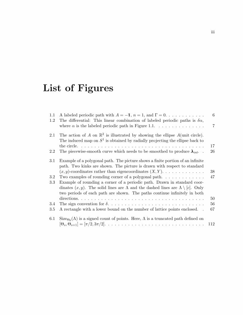
List of Figures
1.1 A labeled periodic path with A = −1, n = 1, and Γ = 0. . . . . . . . . . . . 61.2 The differential: This linear combination of labeled periodic paths is δα,
where α is the labeled periodic path in Figure 1.1. . . . . . . . . . . . . . . 7
2.1 The action of A on R2 is illustrated by showing the ellipse A(unit circle).The induced map on S1 is obtained by radially projecting the ellipse back tothe circle. . . . . . . . . . . . . . . . . . . . . . . . . . . . . . . . . . . . . . 17
2.2 The piecewise-smooth curve which needs to be smoothed to produce λλλint. . 26
3.1 Example of a polygonal path. The picture shows a finite portion of an infinitepath. Two kinks are shown. The picture is drawn with respect to standard(x, y)-coordinates rather than eigencoordinates (X,Y ). . . . . . . . . . . . . 38
3.2 Two examples of rounding corner of a polygonal path. . . . . . . . . . . . . 473.3 Example of rounding a corner of a periodic path. Drawn in standard coor-
dinates (x, y). The solid lines are Λ and the dashed lines are Λ \ [c]. Onlytwo periods of each path are shown. The paths continue infinitely in bothdirections. . . . . . . . . . . . . . . . . . . . . . . . . . . . . . . . . . . . . . 50
3.4 The sign convention for δ. . . . . . . . . . . . . . . . . . . . . . . . . . . . . 563.5 A rectangle with a lower bound on the number of lattice points enclosed. . 67
6.1 SizeΘ0(Λ) is a signed count of points. Here, Λ is a truncated path defined on[Θs,Θs+1] = [π/2, 3π/2]. . . . . . . . . . . . . . . . . . . . . . . . . . . . . . 112

iv
Acknowledgments
I would like to thank my adviser, Michael Hutchings, who helped me to a degree
far beyond the call of duty. I’m deeply grateful. He was helpful at every level, with the
mathematics, writing, bureaucracy, and job search, and by giving me funding. I’m especially
grateful for one of the smallest things he did: He told me not to read a paper all the way
through before starting research.
I’ve been helped in many ways by many people, and I’d especially like to thank Su-
san Amrose, Tathagata Basak, Ushnish Basu, Jennifer Berg, Adam Booth, Carol Bohmer,
Richard Bohmer, Ian Bourg, Jeff Brown, Thomas Brown, Joe Chernick, Michael Christ,
Chris Chun, Andy Cotton-Clay, Dennis Courtney, Cordelia Csar, Elizabeth Dan-Cohen,
Ishai Dan-Cohen, Caleb Deng, Sachin Deshmukh, Polina Dimova, Hanh Do, Tom Dorsey,
Arthur Edelstein, Alyosha Efros, David Farris, Rachel Findley, Ryan Firestone, Johanna
Franklin, Nina Gabelko, Ori Ganor, Fernand Garin, Peter Gerdes, Piotr Gibas, John
Goodrick, Alfonso Gracia-Saz, Ole Hald, Tamas Kalman, Aathavan Karunakaran, Rob
Kirby, Allen Knutson, Andrew Lawrence, David Lebow, Ned Lebow, Kate Lebow, Rob
Letzler, Minh Lim, Ai-ko Liu, Grace Lyo, Maryanthe Malliaris, Sunanda Marella, Alice
Medvedev, Raj Mehta, May Mei, Daphna Michaeli, Dave Mina, Hitoshi Murayama, Thom-
son Nguyen, Madhav Pai, Koushik Pal, Medha Pathak, Seemantini Pathak, Barbara Peavy,
Kathleen Phu, Joaquin Rosales, Jarek Rudzinksi, Kathy Santos, Chung-chieh Shan, Marsha
Snow, Susan Sonoda, Vikrant Sood, Dave Spivak, Betsy Stovall, Katalin Takacs, Makiko
Takekuro, Mel Terry, Dylan Thurston, Akiko To, Dan Volmar, Miraim Walker, Barb Waller,
Judie Welch, Alex Woo, Guoliang Wu, Adena Young, Elizabeth Zacharias, Marco Zambon,

v
and Chenchang Zhu.
1
Chapter 1
Introduction
1.1 Embedded contact homology
Embedded contact homology (ECH), introduced in [5, §1.1 and §11], [6, §7] from
ideas implicit in [3, 4], associates a graded Abelian group ECH∗(Y, λ,Γ) to a 3-manifold
Y , a contact form λ, and a homology class Γ ∈ H1(Y ). A contact form on a 3-manifold is
a 1-form λ such that λ ∧ dλ > 0. The contact form gives rise to the 2-plane field ker(λ),
the contact structure, which is oriented by dλ. The contact form also gives rise to a vector
field R characterized by λ(R) = 1 and R y dλ = 0, the Reeb vector field. A Reeb orbit is a
periodic orbit of the flow of the Reeb vector field.
The ECH of (Y, λ,Γ) is the homology of a chain complex generated by certain
collections of embedded closed (nondegenerate) Reeb orbits in Y . Specifically, a generator
of the chain complex is a collection (with multiplicity) of Reeb orbits, a hyperbolic Reeb
orbit can only appear with multiplicity 1, and the sum (with multiplicity) of the homology
of the Reeb orbits is constrained to be Γ. The matrix coefficient of the differential between
CHAPTER 1. INTRODUCTION 2
two generators counts certain embedded J-holomorphic curves in Y × R, for a suitable
almost complex structure J . (In addition to embedded curves, the count includes unions
of embedded curves with multiple covers of “trivial cylinders” of the form β × R, where
β is a Reeb orbit.) More precisely, the differential counts curves with ends at ±∞ at the
appropriate collections of Reeb orbits, modulo the symmetry of translating a curve in the
R direction of Y × R.
The embedded contact homology of Y is conjectured [5, §1.1] to be isomorphic
to versions of the Seiberg-Witten Floer homology ( ˇHM∗) and the Ozsvath-Szabo Floer
homology (HF+∗ ) of −Y (see [7, 9, 8]). The conjectural isomorphism with Seiberg-Witten
Floer homology is a three-dimensional analogue of Taubes’ SW = Gr result [10, 11]. ECH
is similar (but not isomorphic) to Symplectic Field Theory [1], which counts curves that
need not be embedded.
Taubes has announced a proof ([13], following work in [12]) that ECH is isomorphic
to Seiberg-Witten Floer homology. It follows that ECH is well-defined: ECH is independent
of the extra choices involved in computing it. In particular, it does not depend on the contact
form; it only depends on Y , Γ, and the contact structure (and in fact only on Y , Γ, and
the Euler class of the contact structure).
The purpose of the present work is to compute ECH for a large family of T 2-
bundles over S1. This generalizes the T 3 case, which was computed by Hutchings and
Sullivan [5]. The methods of the current work generalize those of [5]. Hutchings has used
methods similar to the T 3 case in order to compute the ECH of S1×S2. (See [5, §12.2.1] for
the statement of the result.) Other direct calculations of ECH include an easy calculation
CHAPTER 1. INTRODUCTION 3
for S3 by Hutchings [unpublished] and work in progress by David Farris on circle bundles.
1.2 Torus bundles over the circle
An element A of SL2(Z) gives a map T 2 → T 2 and thus a mapping torus
YA = T 2 × [0, 1] / (( xy ) , 0) ∼ (A ( xy ) , 1). (1.1)
(We will use coordinates (x, y) on the T 2 fibers and t on the base S1.) We classify A ∈
SL2(Z), using the rank of A−1. The rank 1 case is the positive parabolic case, and the full
rank case may be further classified: A is hyperbolic if A has distinct real eigenvalues, negative
parabolic if A has only one eigenvalue (necessarily −1), and elliptic if A has imaginary
eigenvalues. We say A is positive hyperbolic if it is hyperbolic with positive eigenvalues, and
similarly for negative hyperbolic.
We compute the ECH of (YA, λn,Γ), where:
• YA is the mapping torus of the action of A ∈ SL2(Z) on T 2, where A is hyperbolic or
−1
and
• n is a positive integer, and the contact form λn (which we construct in Chapter 2) is
of the form a(t) dx+ b(t) dy. Its Reeb vector field is tangent to the T 2 fibers. As one
travels once around the base S1, the Reeb vector field turns counterclockwise through
an angle Nπ (as do the contact planes), where N = 2n if A is positive hyperbolic and
N = 2n− 1 if A is negative hyperbolic or −1.
CHAPTER 1. INTRODUCTION 4
(In fact, λn is Morse-Bott, and we must perturb each circle of Reeb orbits into
two nondegenerate orbits, one elliptic and one hyperbolic. See [5, §11.2.3].)
Note that in our situation the ECH vanishes unless the homology class Γ lies in
the subspace of H1(YA) coming from the homology of a fiber, because all Reeb orbits lie
in the fibers. Henceforth, assume Γ lies in that subspace. Identifying H1(T 2) with Z2, we
then have Γ ∈ Z2/ Im(1 − A), because there is a short exact sequence (coming from the
long exact sequence of a mapping torus [2, p.151 Example 2.48, or p. 158 Exercise 30])
0→ H1(T 2)1−A
ι→ H1(YA)→ H0(T 2)→ 0 (1.2)
in which the map ι is induced by the inclusion of a fiber T 2 into YA.
In general, ECH has a non-canonical grading over Z/m, where m is the divisibility
of the image of c1(ξ) + 2PD(Γ) in Hom(H2(Y ),Z) (here ξ is the contact structure of λ).
The grading is canonical if Γ = 0. In our case, m = 0, and thus ECH has a grading over Z
if Γ = 0 and over a Z-torsor if Γ 6= 0.
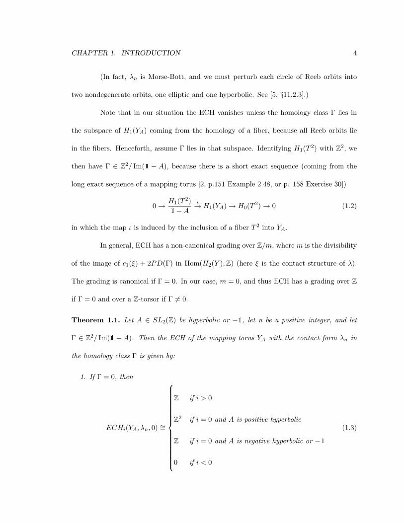
Theorem 1.1. Let A ∈ SL2(Z) be hyperbolic or −1, let n be a positive integer, and let
Γ ∈ Z2/ Im(1 − A). Then the ECH of the mapping torus YA with the contact form λn in
the homology class Γ is given by:
1. If Γ = 0, then
ECHi(YA, λn, 0) ∼=
Z if i > 0
Z2 if i = 0 and A is positive hyperbolic
Z if i = 0 and A is negative hyperbolic or −1
0 if i < 0
(1.3)
CHAPTER 1. INTRODUCTION 5
2. If Γ 6= 0, then ECH∗(YA, λn,Γ) is graded over a Z-torsor which contains i0 such that
ECHi(YA, λn,Γ) ∼=
Z if i ≥ i0
0 if i < i0
(1.4)
The result is independent of the contact form λn. This independence was expected,
from the conjectured isomorphism with Seiberg-Witten Floer homology, and independence
will follow from Taubes’ proof of that conjecture [13]. In the present work, we prove directly
that ECH∗(YA, λn,Γ) ∼= ECH∗(YA, λn+1,Γ) (Chapter 8).
The result is nearly independent of A, which was not expected.
1.3 The method of proof: Polygonal paths
To prove Theorem 1.1, following [5], we give a combinatorial description of a chain
complex whose homology is ECH. The bulk of the present work is devoted to computing
the homology of this combinatorial chain complex.
Fix A, n, and Γ as in Theorem 1.1. The combinatorial chain complex is generated
by labeled periodic paths, certain polygonal paths in R2 with vertices in Z2, with some extra
data. To wit, such a path turns counterclockwise, it satisfies the “periodicity” condition
(∗) below, and each edge carries an ‘e’ or ‘h’ label. Each edge also carries an angle in R,
a lift from S1 of the direction the edge is pointing in, and “counterclockwise” means that
these angles are strictly increasing. The differential δ on the combinatorial chain complex
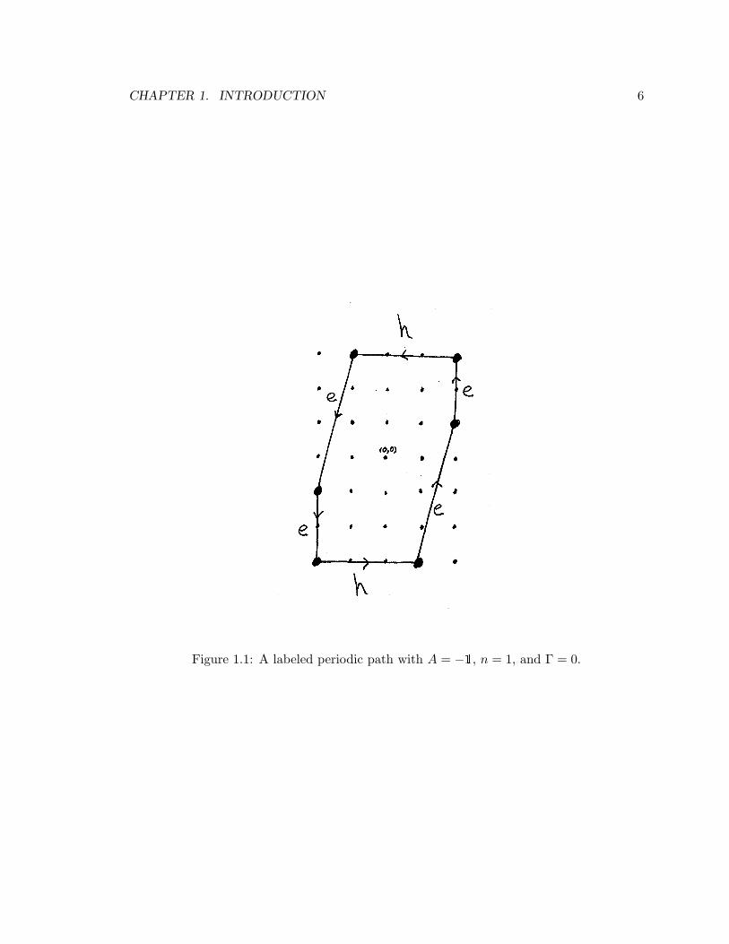
is a signed sum of ways to “round a corner” while “locally losing one ‘h’.” Figure 1.1 shows
an example of a labeled periodic path α, and Figure 1.2 shows the result of applying the
differential to α. We will discuss both figures below.
CHAPTER 1. INTRODUCTION 6
Figure 1.1: A labeled periodic path with A = −1, n = 1, and Γ = 0.

CHAPTER 1. INTRODUCTION 7
Figure 1.2: The differential: This linear combination of labeled periodic paths is δα, whereα is the labeled periodic path in Figure 1.1.
CHAPTER 1. INTRODUCTION 8
The periodicity condition is a relation between an edge at angle θ and an edge at
approximately θ+Nπ. (Angles will always be in R, not S1. Recall that the Reeb vector field
turns through an angle Nπ.) More correctly, the condition uses the function fA,n : R→ R,
a lift to R of the natural action of A on S1 ⊂ R2, and fA,n is the unique such lift satisfying
fA,n(θ0) = θ0 +Nπ for(
cos θ0sin θ0
)an eigenvector of A.
Fix a representative γ ∈ Z2 of Γ ∈ Z2/ Im(1 − A), so Γ = [γ] = γ + Im(1 − A).
We choose γ = 0 if (and only if) Γ = 0. We can now state the periodicity condition:
(∗) If a path has an edge with angle θ starting at a point ( xy ), then the path has an edge
with angle fA,n(θ) starting at A ( xy ) + γ, with the same ‘e’ or ‘h’ label. If a path does
not have an edge with angle θ then it does not have an edge with angle fA,n(θ).
Thus, every time a path turns through an angle of approximately Nπ, it travels
from some ( xy ) to A ( xy ) + γ. (The choice of γ will not affect the homology–different repre-
sentatives of the same Γ yield isomorphic combinatorial chain complexes. See Remark 3.9.)
Figure 1.1 shows an example of a labeled periodic path α, with A = −1, n = 1,
and Γ = 0. Thus, N = 1, γ = 0, and fA,n(θ) = θ + π. In this case, we obtain a polygon
symmetric under rotation by π about the origin. The polygonal path traverses the polygon
infinitely many times. (This phenomenon is quite unlike the hyperbolic case, in which a
path tends to a line parallel to an eigenvector of A as θ → +∞, and tends to a line parallel
to the other eigenvector as θ → −∞.) Figure 1.2 shows δα. Note that corners of α with
both adjacent edges labeled ‘e’ do not contribute to δα. Also, a family of corners identified
by periodicity – opposite corners in the picture – are all rounded at once.
Each labeled periodic path encodes a collection of Reeb orbits. One edge (at angle
CHAPTER 1. INTRODUCTION 9
θ) can be thought of as describing the Reeb orbits in one fiber of the cover T 2 × R of YA
(namely the fiber T 2 × {θ}), and the periodicity condition (∗) ensures that the resulting
collection of Reeb orbits descends to YA. The ‘e’/‘h’ label has to do with elliptic/hyperbolic
Reeb orbits.1 The condition (∗) also enforces the total homology Γ of the collection of Reeb
orbits. (See Appendix A or [5] for more details.)
The combinatorial chain complex is described in detail in Chapter 3. It was intro-
duced in [5, §12.2.2], generalizing the chain complex used in the body of [5] to compute the
ECH of T 3.
Chapters 4–8 compute the homology of the combinatorial chain complex. In par-
ticular, they (and Chapter 3) are purely combinatorial. Here is an outline of the body of
this work.
• The contact form λn is constructed in Chapter 2.
• The combinatorial chain complex, denoted by C∗(A,n, γ), is defined in Chapter 3.
• Chapter 4 defines subcomplexes, C∗(B), of the combinatorial chain complex, involving
paths enclosed by a box or strip B.
• Flattened subcomplexes of C∗(B), with homology isomorphic to H∗(B), are defined in
Chapter 5. The flattened subcomplexes involve paths “maximal” with respect to B.
• Chapter 6 shows that the homology H∗(B) coming from a strip B is isomorphic to
H∗(A,n, γ).
• We compute H∗(A, 1, γ) in Chapter 7.1Strictly speaking, the Reeb orbits of the Morse-Bott contact form λn lie in the T 2 fibers, and the Reeb
orbits of perturbed contact forms are elliptic or hyperbolic.
CHAPTER 1. INTRODUCTION 10
• Chapter 8 shows that H∗(A,n, γ) is independent of n.
• The isomorphism between the embedded contact homology ECH∗(YA, λn,Γ) and the
combinatorially defined homology H∗(A,n, γ) is proved in Appendix A.
1.4 Future work
It seems that the ECH of the mapping torus YA can also be computed when A
is elliptic or negative parabolic, and the result has the same form as that for negative
hyperbolic A. The preliminary calculation was done by David Farris and the author in the
elliptic case, and by the author in the negative parabolic case.
ECH in the positive parabolic case (other than A = 1) has not been computed.
11
Chapter 2
The manifolds YA and their contact
structures
Fix a matrix A ∈ SL2(Z) which is hyperbolic or −1, and a positive integer n. The
purpose of this chapter is to construct a contact form λn on the torus bundle YA, with the
properties described in §1.2. The remaining chapters are combinatorial and independent
of this chapter, except for Appendix A, which relates the combinatorics to the ECH of
(YA, λn). However the notation fA,n introduced below in Lemma-Definition 2.13 will be
needed in the combinatorial chapters.
In §2.1, we restate in coordinates the definition of the manifold YA. In §2.2, we
describe the contact forms λn. The contact planes are “perpendicular” to the fibers, are
constant on any fiber, and rotate by an amount Nπ as one travels once around the base. We
start with the contact forms λn for A = −1, and with that motivation, we give the more
complicated statement of the existence of λn for A hyperbolic. To make that statement
CHAPTER 2. THE MANIFOLDS YA AND THEIR CONTACT STRUCTURES 12
precise, we define the map on lifted angles fA,n. Finally, in §2.3, we prove Proposition 2.8,
constructing λn for A hyperbolic. The construction follows the suggestion in [5, §12.2.2].
2.1 YA and Γ ∈ H1(YA)
The smooth 3-manifolds YA we study are total spaces of 2-torus bundles over the
circle (mapping tori).
Definition 2.1. Let A ∈ SL2(Z), choose coordinates x and y on T 2 in the usual way, and
define
φt((x
y
), t) = (A
(x
y
), t+ 1) (2.1)
so that
YA = T 2 × R/φt. (2.2)
We also write(xy
)as (x, y). (The subscript on φt is to distinguish it from φθ, to
be introduced in a change of coordinates in §2.2. We suppress the dependence of φt on A.)
The monodromy of the bundle is A−1, and we call A the inverse monodromy. Conjugate
matrices give the same bundle. The matrix A acts naturally on R2, its subset Z2, and its
quotient T 2 (and we have identified H1(T 2) with Z2).
Definition 2.2. If A ∈ SL2(Z) is hyperbolic or −1, denote the eigenvalues by a and a−1,
with |a| ≥ 1.

CHAPTER 2. THE MANIFOLDS YA AND THEIR CONTACT STRUCTURES 13
2.2 The contact forms λn and the map fA,n on lifted angles
2.2.1 λn for A = −1
Choose coordinates x and y on T 2 in the usual way (making T 2 ∼= R2/Z2), and a
coordinate θ on R. (Eventually, S1 will be the quotient of R by a certain map fA,n.) We
begin with A = −1, where the form may be defined by a simple equation. Equation (2.3)
below, though correct only for A = −1, also gives the correct intuition for hyperbolic A.
Tildes denote objects on the cover T 2 × R of YA.
Lemma-Definition 2.3. Let
λ = cos θ dx + sin θ dy (2.3)
on T 2 × R. This is a contact form. The Reeb vector field of λ is
R = cos θ∂
∂x+ sin θ
∂
∂y. (2.4)
Proof. By direct calculation, the reader may verify that λ ∧ dλ > 0 if we choose the correct
orientation (so λ is a contact form on T 2 × R) and that λ(R) = 1 and R y dλ = 0 (so R is
its Reeb vector field).
Lemma 2.4. The manifold Y−1, as in Definition 2.1, can also be written as:
Y−1 ∼= (T 2 × R)/φθ (2.5)
φθ((x, y), θ) = ((−x,−y), θ + (2n− 1)π). (2.6)
CHAPTER 2. THE MANIFOLDS YA AND THEIR CONTACT STRUCTURES 14
Proposition 2.5. For all positive integers n, the form λ on T 2 × R descends to a contact
form λn on the quotient Y−1, and R descends to its Reeb vector field.
Proof. We see that φθ respects λ and therefore R. Thus λ and R descend to a contact form
λn and its vector field Rn on Y−1.
Note that the parameterization makes Y−1 a bundle over S1 = R/(2n− 1)πZ. In
particular, λn depends indirectly on n, because the parameterization depends on n. (We
suppress the dependence of φθ on n and A.) The contact planes turn through (2n− 1)π =
Nπ.
2.2.2 λn for hyperbolic A
Some generalizations of Theorem 2.5 are easy.
Example 2.6 (Elliptic A). If A is the rotation matrix that rotates by π/2, we need only
replace Equation (2.6) with
φθ((x, y), θ) = (A(x, y), θ +π
2+ 2π(n− 1)); (2.7)
everything else remains the same. The map θ 7→ θ + π2 + 2π(n− 1) accounts for how much
the contact form turns as we travel once around the base S1, and must be addition of π/2
(up to multiples of 2π) because A rotates by π/2. We call this map fA,n.
Hyperbolic A have a more complicated fA,n, and also change the lengths of vectors
and covectors. For these reasons, we start with a form parameterized by t, not θ. We defer
fA,n, but we define N , because fA,n is approximately addition of Nπ. Instead of expressions
such as cos θ ∂∂x +sin θ ∂
∂y , we will have a vector (Rx(t), Ry(t)) that rotates counterclockwise.

CHAPTER 2. THE MANIFOLDS YA AND THEIR CONTACT STRUCTURES 15
Definition 2.7. If A is positive hyperbolic, we write
N = 2n (2.8)
If A is negative hyperbolic or A = −1,
N = 2n− 1. (2.9)
The quantity Nπ is sometimes called the rotation number fA,n, and the rotation
number may be defined abstractly for all A ∈ SL2(Z). Note that n is the number of
revolutions, rounded up to an integer:
n = drotation number/2πe. (2.10)
Recall that YA is the quotient of T 2 × R by
φt((x, y), t) = (A(x, y), t+ 1). (2.11)
Proposition 2.8. For all hyperbolic A ∈ SL2(Z), and all positive integers n, there is a
1-form λ = λx(t) dx+ λy(t) dy on T 2 × R (with coordinates ((x, y), t)) such that
1. The form λ is a contact form.
2. The form λ descends to a form, called λn, on the quotient YA.
3. The Reeb vector field of λ can be written
R = Rx(t)∂
∂x+Ry(t)
∂
∂y, (2.12)
where the argument θ of (Rx(t), Ry(t)) ∈ R2 satisfies θ′(t) > 0.

CHAPTER 2. THE MANIFOLDS YA AND THEIR CONTACT STRUCTURES 16
4. The argument θ of (Rx(t), Ry(t)) increases by Nπ as t goes from 0 to 1. At t = 0 and
t = 1, (Rx(t), Ry(t)) is an eigenvector of A.
We defer the proof to §2.3. Proposition 2.8 should generalize in a straightforward
way to all A ∈ SL2(Z), but we will work only with hyperbolic matrices and −1.
Note (for well-definedness) that we have only made claims about θ(t) that are
unchanged by adding some t-independent 2πk.
It will turn out that θ increases from an appropriate θ0 to θ0 +Nπ as we go once
around YA.
Since θ′(t) > 0, we may reparameterize everything appearing in Proposition 2.8 as
functions of θ instead of t. The result will be Proposition 2.16.
2.2.3 fA,n for A ∈ SL2(Z)
We need to view the base S1 of the bundle as the quotient of R by a map fA,n : R→
R, so that S1 = R/fA,n (or more formally, we quotient by the infinite cyclic group 〈fA,n〉).
The map fA,n will satisfy fA,n(θ) > θ for all θ ∈ R, to make a good quotient, and fA,n will
be defined in terms of the action of A on angles in R2, as suggested by our notation θ.
Notation Convention 2.9. Any matrixA ∈ SL2(Z) acts on R2 inducing a mapAS1 : S1 →
S1, obtained as the composition
S1 ↪→ R2 \ {0} A→ R2 \ {0}� S1, (2.13)
or more abstractly by viewing this S1 as (R2 \ {0})/R+, the set of directions in R2.
See Figure 2.1. To obtain fA,n, we will lift AS1 to a map on the universal cover R
of S1.

CHAPTER 2. THE MANIFOLDS YA AND THEIR CONTACT STRUCTURES 17
Figure 2.1: The action of A on R2 is illustrated by showing the ellipse A(unit circle). Theinduced map on S1 is obtained by radially projecting the ellipse back to the circle.
Definition 2.10. The copy of R that is the universal cover of S1 = (R2 \ {0})/R+ is called
the space of lifted angles, or just angles.
Note that this R will have two different quotients:
• The circle S1, the space of directions in R2, is the quotient R/2πZ.
• The S1 that is the base of the bundle YA is the quotient R/fA,n.
Definition 2.11. A lift of AS1 is a map f : R → R such that π ◦ f = AS1 ◦ π where π is
the projection to the quotient, π : R→ R/2πZ.
In other words, A(cos θ, sin θ) is a positive θ-dependent multiple of (cos f(θ), sin f(θ)).
Lemma 2.12. Any two lifts f, f are related by f = f + 2πn for some n ∈ Z, and each lift
f of AS1 satisfies
f(θ + 2π) = f(θ) + 2π. (2.14)

CHAPTER 2. THE MANIFOLDS YA AND THEIR CONTACT STRUCTURES 18
Proof. Lifts of AS1 exist, adding 2πn (n ∈ Z) yields another lift, and all lifts of AS1 are of
this form. To show (2.14), note that AS1 and its lifts make sense not just for A ∈ SL2(Z),
but also for A ∈ SL2(R), which is connected. For any A ∈ SL2(R) and any lift f of AS1 ,
we may obtain a lifted homotopy from f to a lift g of 1S1 , specifically g(θ) = θ + 2πk for
some k ∈ Z. On that homotopy, for any θ ∈ R, f(θ + 2π) − f(θ) ∈ 2πZ does not change,
reaching g(θ + 2π)− g(θ) = 2π. So f(θ + 2π)− f(θ) = 2π as claimed.
We will now define maps on lifted angles, and we will let fA,n be the “n’th smallest”
of them.
Lemma-Definition 2.13. For any A ∈ SL2(Z):
• Definition: A map on lifted angles is a map f : R → R which is a lift of AS1 , and
which satisfies
f(θ) > θ for all θ ∈ R. (2.15)
• Claim: There is a smallest map on lifted angles (which we denote fA,1) under the
relation that f is smaller than f if and only if f + 2πk = f where k > 0.
• Definition: We let
fA,n(θ) = fA,1(θ) + 2π(n− 1), n = 1, 2, 3, . . . . (2.16)
• Claim: The maps on lifted angles are precisely the maps fA,n for n a positive integer.
Proof. Equation (2.14) shows that f(θ)− θ is periodic, so bounded.
Among lifts f of AS1 , the subset satisfying (2.15) is neither all lifts nor empty,
because adding sufficiently negative 2πn to any given lift produces violations of (2.15),

CHAPTER 2. THE MANIFOLDS YA AND THEIR CONTACT STRUCTURES 19
and adding sufficiently large positive 2πn produces f satisfying (2.15) (since f(θ) − θ is
bounded). Thus there is a smallest map on lifted angles. So all maps on lifted angles must
be of the form (2.16), and these are all the maps on lifted angles since adding positive
constants preserves (2.15).
2.2.4 fA,n for hyperbolic A
Example 2.14. For any positive hyperbolic A, we show an example of a lift f0 which is
not a map on lifted angles. See Figure 2.1. The map AS1 fixes the elements of S1 on
each eigenline (1-dimensional eigenspace). For any θ0 ∈ R “pointing along an eigenline”
(i.e., mapping to one of the fixed elements of S1, or in other words, with (cos θ0, sin θ0) an
eigenvector of A), there is a unique f0 (shown) such that f0(θ0) = θ0. Then this f0 fixes all
θ0 that point along an eigenline. We see that there exist θ with f0(θ) < θ.
We will show fA,1(θ) = f0(θ) + 2π (and fA,n(θ) = f0(θ) + 2πn). We will have
fA,n(θ0) = θ0 + 2πn for θ0 pointing along an eigenline, (2.17)
even though fA,n has more complicated behavior for general θ. To show that fA,1 is what
we claim, we will need the fact that f0 displaces any θ by less than π, i.e. |f0(θ)− θ| < π for
all θ, which is evident from the fact that f0 does not move any angle past any eigenline.
Lemma 2.15. If A is hyperbolic or A = −1, and(
cos θ0sin θ0
)is an eigenvector of A, then
fA,n(θ0) = θ0 +Nπ.
Proof. If A is positive hyperbolic we have f0 from Figure 2.1, a lift of AS1 which cannot
be a map on lifted angles. Clearly, f0 + 2π is a map on lifted angles, and is therefore fA,1,

CHAPTER 2. THE MANIFOLDS YA AND THEIR CONTACT STRUCTURES 20
giving
fA,n(θ) = f0(θ) + 2πn. (2.18)
Thus, fA,n(θ0) = θ0 + 2πn.
If A is negative hyperbolic or −1, we may use the lift f0 of (−A)S1 . Then f0 +π is
a lift of AS1 and satisfies f0(θ)+π > θ, so it is a map on lifted angles. However, f0(θ)−π < θ
so f0 − π is not a map on lifted angles. Thus fA,1 = f0 + π and fA,n = fA,1 + 2π(n− 1) =
f0 + (2n− 1)π. So fA,n(θ0) = θ0 + (2n− 1)π.
Proposition 2.16. Reparameterizing the R of T 2×R by θ (the argument of (Rx, Ry) from
Proposition 2.8) instead of t yields
YA = T 2 × R/φθ (2.19)
φθ((x, y), θ) = (A(x, y), fA,n(θ)), (2.20)
and the Reeb vector field on T 2×R is (cos θ ∂∂x + sin θ ∂
∂y ) times a positive real function of θ.
Here we have made an (arbitrary) choice of a particular smooth function θ(t)
giving the argument of (Rx, Ry), among the Z-family of such choices.
Proof. We may reparameterize by Proposition 2.8, part 3, and part 4 insures that θ ranges
over all of R. That the Reeb field is proportional to the given field is just what it means
to reparameterize by the argument θ. We must show that t 7→ t+ 1 becomes θ 7→ fA,n(θ).
Define f by f(θ(t)) = θ(t+ 1). We first show that f is a lift of AS1 , and then that f is the
lift fA,n.
We have φ∗t λ = λ, so (φt)∗R = R, or in other words
A(Rx(t), Ry(t)) = (Rx(t+ 1), Ry(t+ 1)). (2.21)
CHAPTER 2. THE MANIFOLDS YA AND THEIR CONTACT STRUCTURES 21
For each t, we have that (Rx(t), Ry(t)) is a positive real multiple of (cos θ, sin θ), which we
denote
(Rx(t), Ry(t)) ∝ (cos θ(t), sin θ(t)). (2.22)
Then
(Rx(t+ 1), Ry(t+ 1)) ∝ (cos θ(t+ 1), sin θ(t+ 1)) = (cos f(θ(t)), sin f(θ(t))), (2.23)
so
A(cos θ(t), sin θ(t)) ∝ A(Rx(t), Ry(t)) = (Rx(t+ 1), Ry(t+ 1)) ∝ (cos f(θ(t)), sin f(θ(t))),
(2.24)
i.e.
AS1(cos θ(t), sin θ(t)) = (cos f(θ(t)), sin f(θ(t))) (2.25)
(see Notation Convention 2.9). But θ 7→ (cos θ, sin θ) is exactly the projection π : R →
R/2πZ from Definition 2.11, so (AS1 ◦ π)(θ(t)) = (π ◦ f)(θ(t)) for all t. Thus f is a lift of
AS1 .
Recall that fA,n is defined to be the n’th-smallest lift of AS1 satisfying f(θ) > θ.
It is clear that f satisfies f(θ) > θ, because it was obtained by conjugating t 7→ t + 1 by
the order-preserving map θ. So f = fA,k for some positive integer k. Proposition 2.8, part
4 means that θ(0) = θ0 for some θ0 as in Lemma 2.15, and θ(1) = θ0 +Nπ. But
θ(1) = f(θ(0)) = fA,k(θ0), (2.26)
so θ0 + Nπ = fA,k(θ0). Applying Lemma 2.15 shows n = k because different n’s have
disjoint possibilities for N . Thus f = fA,n, as desired.

CHAPTER 2. THE MANIFOLDS YA AND THEIR CONTACT STRUCTURES 22
Remark 2.17. Each closed Reeb orbit in T 2 × R lies in some fiber T 2 × {θ} where θ has
rational slope, tan θ ∈ Q ∪ {∞}, and each such T 2 fiber contains a family of Reeb orbits.
We are in the Morse-Bott case, and in Appendix A, we will perturb the contact
form in a neighborhood of such a fiber to have only one elliptic and one hyperbolic Reeb
orbit.
2.3 Proof of Proposition 2.8
We prove Proposition 2.8 by constructing a curve λλλ(t) = (λx(t), λy(t)) satisfying
appropriate conditions. The conditions will include det(λλλ,λλλ′) > 0, which means the vector
λλλ(t) “turns counterclockwise”. Here, ′ is just the t derivative, and det(a,b) = axby − aybx
is the familiar two-dimensional analog of the cross product.
Lemma 2.18. The argument arg(a) of a(t) satisfies arg(a)′ > 0 if and only if det(a,a′) > 0.
Proof. We have det(a,a′) = |a|2arg(a)′.
Lemma 2.19. To prove Proposition 2.8, it is sufficient that λλλ(t) = (λx(t), λy(t)) be a
smooth function R→ R2 satisfying:
1. For all t, det(λλλ(t),λλλ′(t)) > 0.
2. For all t,
λλλ(t+ 1) = (AT )−1λλλ(t). (2.27)
3. For all t, det(λλλ′(t),λλλ′′(t)) > 0.
4. a) The argument of λλλ′(t) increases by the amount Nπ as t goes from 0 to 1.
CHAPTER 2. THE MANIFOLDS YA AND THEIR CONTACT STRUCTURES 23
b) The vector λλλ′(t) is an eigenvector of (AT )−1 at t = 0 and t = 1.
Note that we use A for periodicity of (Rx(t), Ry(t)) ∈ R2, but the inverse transpose
(AT )−1 for (λx(t), λy(t)); if we were being more picky, we would say λλλ(t) ∈ (R2)∗. Of course,
AT and (AT )−1 have the same eigenvectors.
Proof. We show part i of Proposition 2.8 from part i of Lemma 2.19, sometimes assuming
earlier parts of Lemma 2.19.
1. We need λ ∧ dλ > 0. We have
λ ∧ dλ = (λx dx+ λy dy) ∧ (λ′x dt ∧ dx+ λ′y dt ∧ dy) (2.28)
= λxλ′y dt ∧ dy ∧ dx− λyλ′x dt ∧ dy ∧ dx (2.29)
= det(λλλ,λλλ′) vol (2.30)
where we are using the same (unintuitive) orientation on T 2 × R as we did for Y−1.
2. We need
φ∗t λ = λ. (2.31)
Converting this equation from λ to λλλ using the definition of pullback and the definition
(2.11) of φt yields ATλλλ(t+ 1) = λλλ(t), which follows from (2.27).
3. We first determine the Reeb vector field in terms of λλλ(t) (a result also found in [5,
§10.4]).
Lemma 2.20. If λx(t) dx+λy(t) dy is a contact form on T 2×R, its Reeb vector field
is R = Rx(t) ∂∂x +Ry(t) ∂∂y where
R(t) = (Rx(t), Ry(t)) =1
det(λλλ(t),λλλ′(t))(λ′y(t),−λ′x(t)). (2.32)

CHAPTER 2. THE MANIFOLDS YA AND THEIR CONTACT STRUCTURES 24
Proof. The given curve R satisfies 1 = λλλ ·R and 0 = R · λλλ′, which means that the
given vector field satisfies 1 = λ(R) and 0 = R y dλ.
We must show that R(t) has θ′(t) > 0. Denote the argument of λλλ′ by θ, retaining θ
for the argument of R, we have θ′(t) > 0 since det(λλλ′,λλλ′′) > 0. (In particular, this det
condition means λλλ′(t) 6= 0, so we can speak of the argument of λλλ′. Similarly, we have
R(t) 6= 0.)
Lemma 2.21.
θ(t) = θ(t) + π/2 (2.33)
is (one correct choice for) the argument of λλλ′(t).
We say “one correct choice” because adding 2πk produces other correct choices.
Proof. Part 1 of Lemma 2.19 ensures that the 1/ det(λλλ(t),λλλ′(t)) factor of (2.32) is
positive. Further, (λ′y,−λ′x) is just (λ′x, λ′y) rotated by −π/2.
Thus, θ′(t) = θ′(t) > 0.
4. The argument of R increases by the same amount as that of λλλ′ (Lemma 2.21). It
remains only to show that if λλλ′(t) is an eigenvector of (AT )−1, then R(t) is an eigen-
vector of A. Recall that A has distinct real eigenvalues. The dual basis (in (R2)∗) of a
basis of eigenvectors of A forms a basis of eigenvectors of AT , and therefore of (AT )−1.
If λλλ′(t) is an eigenvector of (AT )−1, then R(t), being nonzero and perpendicular to
λλλ′(t), will be an eigenvector of A.

CHAPTER 2. THE MANIFOLDS YA AND THEIR CONTACT STRUCTURES 25
Lemma 2.22. There exists a smooth map λλλ : R → R2 satisfying the conditions given in
Lemma 2.19.
This lemma will complete the proof of Proposition 2.8.
Proof. The idea of this proof is to diagonalize (AT )−1 and then interpolate between C, the
unit circle (in the new coordinates), and the ellipse (AT )−1(C), thus satisfying condition 2
(and also 4b). The interpolation will be made to satisfy conditions 1 and 3, and we will
spend the right amount of time on each curve to satisfy condition 4a.
We diagonalize (AT )−1. We let the X-axis be the a-eigenline (1-dimensional
eigenspace) where |a| > 1, let the Y -axis be the a−1-eigenline. (These coordinates re-
semble, but are not the same as, the eigencoordinates introduced in §3.1.) Thus, the main
ellipse, (AT )−1(C), meets the X-axis at ±a and the Y -axis at ±a−1.
Parameterize C by (cos Θ, sin Θ) and (AT )−1(C) by (AT )−1(cos Θ, sin Θ). (So
Θ is not the argument of some vector.) There exists an interpolation between C and
(AT )−1(C), a smooth curve λλλint : R→ R2 which agrees with C for Θ ∈ (−∞, ε) and agrees
with (AT )−1(C) for Θ ∈ (π/2−ε,∞), and which has λλλint and λλλ′int turning counterclockwise,
i.e. it satisfies det(λλλint,λλλ′int) > 0 and det(λλλ′int,λλλ
′′int) > 0. We may obtain this interpola-
tion by smoothing a piecewise-smooth curve (see Figure 2.2). We would just connect C(ε)
to (AT )−1(C)(π/2 − ε) by a line segment, and smooth the result, but in order to satisfy
det(λλλ′int,λλλ′′int) > 0, i.e. that λλλ′int turns strictly counterclockwise, we first bend the line seg-
ment out slightly to an arc of a very large circle.
Since λλλ′int turns counterclockwise, its argument (in (X,Y )-coordinates) increases
monotonically from π/2 to π as Θ goes from 0 to π/2. Thus as Θ increases from 0 to Nπ,
CHAPTER 2. THE MANIFOLDS YA AND THEIR CONTACT STRUCTURES 26
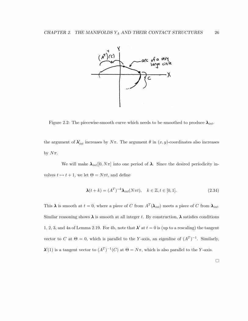
Figure 2.2: The piecewise-smooth curve which needs to be smoothed to produce λλλint.
the argument of λλλ′int increases by Nπ. The argument θ in (x, y)-coordinates also increases
by Nπ.
We will make λλλint|[0, Nπ] into one period of λλλ. Since the desired periodicity in-
volves t 7→ t+ 1, we let Θ = Nπt, and define
λλλ(t+ k) = (AT )−kλλλint(Nπt), k ∈ Z, t ∈ [0, 1]. (2.34)
This λλλ is smooth at t = 0, where a piece of C from AT (λλλint) meets a piece of C from λλλint.
Similar reasoning shows λλλ is smooth at all integer t. By construction, λλλ satisfies conditions
1, 2, 3, and 4a of Lemma 2.19. For 4b, note that λλλ′ at t = 0 is (up to a rescaling) the tangent
vector to C at Θ = 0, which is parallel to the Y -axis, an eigenline of (AT )−1. Similarly,
λλλ′(1) is a tangent vector to (AT )−1(C) at Θ = Nπ, which is also parallel to the Y -axis.

27
Chapter 3
The combinatorial chain complex
C∗(A, n, γ)
This chapter introduces the combinatorial chain complex, C∗(A,n, γ), depending
on A ∈ SL2(Z), hyperbolic or −1; n, a positive integer; and γ ∈ Z2. The homology
H∗(A,n, γ) is isomorphic to ECH∗(YA, λn,Γ). (See Appendix A for details, including how
a generator of C∗(A,n, γ) encodes a generator of the analytical chain complex of ECH.
Throughout this paper, as in [5], we pass from chain complexes to homology by changing
notation from C toH.) In particular, the result is independent of the choice of representative
γ of Γ (see Lemma 3.8 and Remark 3.9).
We start the chapter by changing coordinates on the plane to eigencoordinates of
A in §3.1. We introduce the generators of the combinatorial chain complex, labeled periodic
paths, in §3.2. We start with polygonal paths in §3.2.1, which are counterclockwise-turning
polygonal paths in the plane with vertices in a lattice (the lattice Z2 in standard coordinates
CHAPTER 3. THE COMBINATORIAL CHAIN COMPLEX C∗(A,n, γ) 28
but denoted LA,Γ in eigencoordinates). We define (A,n, γ)-periodic paths, also called just
periodic paths, in §3.2.2. We also introduce the auxiliary notion of truncated path in §3.2.2,
essentially the result of taking just a part of a periodic path. In §3.2.3, we introduce labeled
periodic and truncated paths, labeled with ‘e’ and ‘h’.
The differential is introduced in §3.3, starting with its effect on unlabeled paths
(“rounding a corner”), and then on ‘e’ and ‘h’ labels.
The grading is introduced in §3.4, with an existence/uniqueness proof deferred
until §3.6. It follows the definition in §3.5 of the partial order ≤ on periodic and truncated
paths, which is needed not only for §3.6 but also for the remainder of this work.
The chain complex in this chapter is the generalization (following [5, §12.2.2]) of
the chain complex of [5, §2-3], with a different sign convention, among other minor details.
(There is also the difference that we have chosen γ ∈ Γ, a choice which replaces a quotient
operation by Z2 in defining C∗(A,n; Γ) in [5]. Remark 3.24 has more on this minor point.)
3.1 Change of coordinates
3.1.1 The lattice LA,Γ and coordinate systems (X, Y ) and (x, y)
Recall that the eigenvalues of A are a and a−1, where |a| ≥ 1. Recall that N = 2n
if a A is positive hyperbolic (a > 1), and N = 2n − 1 if A is negative hyperbolic or −1
(a ≤ −1). Thus N ≥ 1.
The generators of C∗(A,n, γ) will be counterclockwise-turning polygonal paths in
the plane, with vertices in a lattice, satisfying a periodicity condition, and with ‘e’ and
‘h’ labels on the edges. (It is only through the lattice and the periodicity condition that
CHAPTER 3. THE COMBINATORIAL CHAIN COMPLEX C∗(A,n, γ) 29
(A,n,Γ) affect the chain complex. See Defintion 3.21 for the full statement of periodicity.)
Writing down the lattice and the periodicity condition requires coordinates, and there are
two convenient choices, related by an affine transformation:
• Standard coordinates (x, y), in which the lattice is Z2 and the periodicity condition
involves xy
7→ A
xy
+ γ, (3.1)
which has a unique fixed point, (1−A)−1γ.
• Eigencoordinates (X,Y ) in which the periodicity condition involvesXY
7→ aX
a−1Y
, (3.2)
and the lattice is not pretty. We use eigencoordinates for the rest of this
dissertation, except when otherwise noted, and in particular, we let 0 denote the
origin (X,Y ) = (0, 0), which is in general different from (x, y) = (0, 0). We
represent angles by the polar coordinate Θ associated to (X,Y ). The point
(X,Y ) = (0, 0) is the fixed point of the transformation (3.2), and corresponds to the
point (1−A)−1γ in standard coordinates, the fixed point of (3.1).
Although standard coordinates are close to the idea of Chapter 2, eigencoordinates
are much more convenient for Chapter 4 and on, and they are just as convenient for the
current chapter.
Construction of Eigencoordinates from Standard Coordinates. • Put the ori-
gin (X,Y ) = 0 at (x, y) = (1−A)−1γ.
CHAPTER 3. THE COMBINATORIAL CHAIN COMPLEX C∗(A,n, γ) 30
• If A is hyperbolic, make the X-axis parallel to an eigenvector of A with eigenvalue a
(|a| > 1), and make the Y -axis parallel to an eigenvector with eigenvalue a−1.
• If A = −1, make the X-axis parallel to an eigenvector of ( 2 11 1 ) with eigenvalue a
(|a| > 1), and make the Y -axis parallel to an eigenvector with eigenvalue a−1. (See
Remark 3.4.)
• Choose the orientation and scale of the X- and Y -axes so that the change of coordi-
nates map, sending the pair of reals (x, y) to the (X,Y ) that refers to the same point,
preserves area and orientation.
Definition 3.1. When being extra careful, we will denote the coordinates of a point p in
the different systems by x(p), y(p), X(p), and Y (p). Normally, though, we will write R2 for
the plane and p = (X,Y ).
We state the formal relation between (3.1) and (3.2):
Lemma 3.2. By construction, for any p = (X,Y ), letting q = (aX, a−1Y ), we havex(q)
y(q)
= A
x(p)
y(p)
+ γ. (3.3)
Eigencoordinates are not quite unique. (For any nonzero b ∈ R, we may compose
with (X,Y ) 7→ (bX, b−1Y ).)
Definition 3.3. For the rest of this work, for each (A,n, γ), fix one choice of eigencoordinate
system.

CHAPTER 3. THE COMBINATORIAL CHAIN COMPLEX C∗(A,n, γ) 31
The choice is just a choice of coordinates; different choices yield isomorphic chain
complexes.
Remark 3.4. We need eigencoordinates for −1 to have some properties in common with
hyperbolic A, most importantly, Proposition 3.6, Part 4. To achieve this, we have made
the X- and Y -axes for A = −1 a translation of those for some hyperbolic A, and to be
definite, we chose A = ( 2 11 1 ). (Our construction also helps with a technical issue appearing
in Lemma 3.75.)
We now consider how the lattice, Z2 in standard coordinates, appears in eigenco-
ordinates.
Definition 3.5. Let the lattice be
LA,Γ = {p = (X,Y ) ∈ R2 | (x(p), y(p)) ∈ Z2}. (3.4)
The notation LA,Γ (rather than LA,γ) is justified by Lemma 3.8.
The point (0, 0) referred to in the next proposition is (X,Y ) = (0, 0), by our
conventions on coordinate systems. It is an important point, being fixed by the affine
transformation (3.2), whereas (x, y) = (0, 0) is unimportant.
Proposition 3.6. 1. A bounded region contains only finitely many points of LA,Γ.
2. The lattice is invariant under(a 00 a−1
):a 0
0 a−1
(LA,Γ) = LA,Γ. (3.5)
3. The point (0, 0) is in LA,Γ if and only if Γ = 0.

CHAPTER 3. THE COMBINATORIAL CHAIN COMPLEX C∗(A,n, γ) 32
4. No two points in LA,Γ have the same X-coordinate and no two have the same Y -
coordinate.
5. No point on the axes, {X = 0} ∪ {Y = 0}, except possibly (0, 0), is in LA,Γ.
Proof. 1. Discreteness is unaffected by a change of coordinates.
2. This claim is a restatement of the invariance of Z2 under (3.1), which in turn follows
because A ∈ SL2(Z).
3. The point (X,Y ) = (0, 0) is the point (x, y) = (1 − A)−1γ, the fixed point of (3.3).
Let CM = (1−A)−1γ. (“CM” for center of mass.) We have (0, 0) ∈ LA,Γ if and only
if CM ∈ Z2. Since γ = (1−A)(CM), CM ∈ Z2 if and only if γ ∈ (1−A)(Z2); since
Γ = [γ] ∈ Z2/ Im(1−A), we have γ ∈ (1−A)(Z2) if and only if Γ = 0.
4. We state the proof only for the X-coordinate. The idea is that the X-axis, seen in
(x, y)-coordinates, has irrational slope and therefore cannot contain two points of Z2.
We must show no two distinct p, q ∈ Z2 lie on a line parallel to the X-axis. If they
were on such a line, we would have p− q parallel to the X-axis, so p− q would be an
eigenvector of A of eigenvalue a, by the construction of the X-axis. Then,
A−k(p− q) = a−k(p− q), k = 1, 2, 3, . . . (3.6)
would all lie in Z2, since A preserves Z2. This contradicts discreteness of Z2.
5. Again, the idea is the irrational slope of the axes. (We may consider just the X-axis.)
An axis cannot contain both (1− A)−1γ ∈ Q2 and a lattice point. The formal proof
CHAPTER 3. THE COMBINATORIAL CHAIN COMPLEX C∗(A,n, γ) 33
is easiest in eigencoordinates: If (X, 0) ∈ LA,Γ, X 6= 0, then
(a 00 a−1
)−kX
0
= a−kX ∈ LA,Γ, (3.7)
contradicting discreteness of LA,Γ.
Remark 3.7. The details of what LA,Γ looks like (in (X,Y ) coordinates) are very unim-
portant; for most of this work, it may as well be an irregular smattering of points, not even
a lattice. It seems likely that the homology coming from any L ⊂ R2 satisfying a few proper-
ties is isomorphic to the homology H∗(A,n, γ) we calculate in this work, with the condition
Γ = 0 in the description of H∗(A,n, γ) replaced by 0 ∈ L. The properties needed are that L
is a discrete subset of R2, satisfying Proposition 3.6, and a result that the points are “dense
enough”, Lemma 3.75. (There is an inessential use of the fact that LA,Γ is a lattice in
Lemma-Definition 3.73.)
Lemma 3.8. The lattice LA,Γ (seen in eigencoordinates) is independent of the choice of
representative γ of Γ ∈ Z2/ Im(1−A).
Proof. If we have two representatives γ, γ′ then γ′ = γ + (1 − A)v for some v ∈ Z2.
Eigencoordinates for γ′ will be centered on the fixed point of ( xy ) 7→ A ( xy ) + γ′, which is
(1−A)−1γ′ = (1−A)−1γ+v. The entire eigencoordinate system will be translated by v, as
seen from standard coordinates; since v ∈ Z2, the translation leaves the coordinate system
in the same place relative to the points of Z2.
Remark 3.9. By Lemma 3.8, the choice of representative γ of Γ does not affect the chain
complex C∗(A,n, γ).
CHAPTER 3. THE COMBINATORIAL CHAIN COMPLEX C∗(A,n, γ) 34
Seen from the point of view of eigencoordinates, different choices of γ yield the same
chain complex, while from the point of view of standard coordinates, they yield isomorphic
chain complexes related by a translation. (The only effect of (A,n, γ) on C∗(A,n, γ) is
through the lattice, the map FA,n, and the affine transformation (3.1) or (3.2).) The name
C∗(A,n, γ) rather than C∗(A,n,Γ) is chosen from the standard coordinates’ point of view.
3.1.2 Angles in eigencoordinates
In eigencoordinates, we use the coordinate Θ for angles when making statements
such as “(X,Y ) = r(cos Θ, sin Θ) with r > 0.” This coordinate Θ parameterizes a certain
line, abstractly the cover of the S1 of directions in R2, the same line parameterized as θ in
standard coordinates.
Recall that the term angle always refers to elements of R, not S1. We sometimes
emphasize this convention by calling angles lifted angles.
The new coordinates have the virtue that an angle “pointing along an eigenline”
of A (as in Chapter 2) points along an axis, i.e. Θ = kπ/2, k ∈ Z. We have no need of θ in
the rest of this work, once we describe the map on lifted angles fA,n(θ) in eigencoordinates
as FA,n(Θ). The following proposition states all we need to know about FA,n.
Proposition 3.10. There exists a unique smooth FA,n : R → R (for each A and n) such
that
1.(a 00 a−1
) (cos Θsin Θ
)is a positive real multiple of
(cosFA,n(Θ)
sinFA,n(Θ)
).
2. FA,n(kπ/2) = kπ/2 +Nπ for k ∈ Z.
3. FA,n(Θ) > Θ.
CHAPTER 3. THE COMBINATORIAL CHAIN COMPLEX C∗(A,n, γ) 35
4. F ′A,n(Θ) > 0.
Proof. Condition 1 states that FA,n is a lift to R = S1 of the map induced by(a 00 a−1
)on
S1 ⊂ R2. (In the notation of §2.2, it is a lift of(a 00 a−1
)S1 .) It is unique once Condition 2
chooses a value for, say, FA,n(0). For existence of FA,n, we refer to the results on fA,n in §2.2,
restating those results in eigencoordinates: Lemma-Definition 2.13 gives us Conditions 1 and
3, Lemma 2.15 gives us Condition 2, and Condition 4 states that FA,n preserves orientation
on R, which follows because the action of(a 00 a−1
)S1 on S1 preserves orientation.
Notation Convention 3.11. For Θ ∈ R, let ~Θ =(
cos Θsin Θ
).
Remark 3.12. We describe the relation between these coordinate systems and YA ∼= T 2 ×
R/ ∼ from Chapter 2. The affine plane in which polygonal paths will live is T 2, with its
quotient T 2 being R2/Z2 in standard coordinates and R2/LA,Γ in eigencoordinates. Letting
V be the vector space associated to the affine space T 2, the set of directions in V forms
(V \ {0})/R+; let P+(V ) denote the universal cover of this circle, with coordinate Θ in
eigencoordinates and θ in standard coordinates. Then YA ∼= T 2 × P+(V )/φ where
• In standard coordinates, φ acts on T 2 by ( xy ) 7→ A ( xy ), and acts on P+(V ) by fA,n.
• In eigencoordinates, φ acts on T 2 by(XY
)7→(a 00 a−1
) (XY
), and acts on P+(V ) by FA,n.
In particular, YA is a bundle over the circle R/fA,n or R/FA,n, which is not the
circle (V \ {0})/R+. A polygonal path in the plane will encode data about a collection of
Reeb orbits (see Appendix A for details), with the periodicity condition on paths involving
FA,n and(a 00 a−1
), ensuring that the Reeb orbits lie in YA, not just T 2 × P+(V ).

CHAPTER 3. THE COMBINATORIAL CHAIN COMPLEX C∗(A,n, γ) 36
3.2 Labeled periodic paths, the generators of C∗(A, n, γ)
3.2.1 Polygonal paths
The kind of path we are really interested in is a periodic path. As a warm-up, we
formalize the notion of a polygonal path, a counterclockwise-turning polygonal path in R2
with vertices in LA,Γ. (We are using eigencoordinates (X,Y ) on R2.)
A polygonal path is sequence of directed line segments, each associated with an
angle Θ ∈ R. A directed line segment automatically has a direction Θ ∈ S1, but we choose
a lift in R.
To be sure of conventions, we define some fairly standard terms.
Definition 3.13. A directed line segment in R2 is a line segment such that one endpoint
is declared the beginning and the other endpoint (which is a different point) is the end.
Definition 3.14. A subset A of R is discrete if A∩B is finite for any bounded B ⊂ R. If
Θ1,Θ2 ∈ A with Θ1 < Θ2, we say Θ2 is the next element of A after Θ1, or equivalently Θ1
is the previous element before Θ2, if A ∩ (Θ1,Θ2) is empty.
If A is discrete and Θ ∈ A is not the largest element, there is a next element, and
similarly for previous.
Definition 3.15. A non-constant polygonal path is a non-empty set Λ of pairs (σ,Θ), called
edges, such that
1. Each σ is a directed line segment in R2, Θ is an angle in R, and the vector from the
beginning of σ to the end is a positive real multiple of (cos Θ, sin Θ). We denote σ by
EdgeΛ(Θ).

CHAPTER 3. THE COMBINATORIAL CHAIN COMPLEX C∗(A,n, γ) 37
2. The set of Θ appearing in Λ, denoted Ang(Λ), is discrete.
3. If Θ1,Θ2 ∈ Ang(Λ) and Θ2 is the next element of Ang(Λ) after Θ1, the end of
EdgeΛ(Θ1) is the beginning of EdgeΛ(Θ2).
4. A vertex is the beginning or end of any σ appearing in Λ. We require each vertex to
lie in the lattice LA,Γ.
(One could regard Λ as a function from Ang(Λ) to edges, but we denote that
function by EdgeΛ(·) because we are reserving Λ(·) for Definition 3.18.)
The empty set would satisfy Definition 3.15 if we had not specifically excluded it.
Definition 3.16. A polygonal path Λ is either a non-constant polygonal path or is the
constant path at p, for some p ∈ LA,Γ:
The constant path at p, denoted constp, is completely specified by the data of a
point p ∈ LA,Γ. We say p is the only vertex of constp, and Ang(constp) is the empty set.
“Counterclockwise-turning” is the one part of the intuitive description of these
paths not apparent from the definition. But Θ is strictly increasing as we travel along the
path, because the definition joins the edge at Θ with the edge at the next-smallest Θ. Often
successive Θ’s differ by ≤ π, and the path turns counterclockwise. Otherwise, we say the
path has a kink :
Definition 3.17. A corner of a polygonal path Λ is a connected component of R\Ang(Λ).
A proper corner is a corner of the form (Θ1,Θ2) with Θ2 − Θ1 ≤ π. If c = (Θ1,Θ2) with
Θ2 −Θ1 > π, or if c = R, we say c is a kink.

CHAPTER 3. THE COMBINATORIAL CHAIN COMPLEX C∗(A,n, γ) 38
Figure 3.1: Example of a polygonal path. The picture shows a finite portion of an infi-nite path. Two kinks are shown. The picture is drawn with respect to standard (x, y)-coordinates rather than eigencoordinates (X,Y ).
A corner lives in R and a vertex in R2. A corner of the form (−∞,Θ) or (Θ,∞)
is not proper (and is not important). If Λ has a kink, we illustrate this by drawing a small
loop. Figure 3.1 illustrates kinks with Θ2−Θ1 = 3π/2 and 5π/2; Θ2−Θ1 can get arbitrarily
large. The constant path has a kink.
Figure 3.1 also shows an edge that is not “primitive”–it has a lattice point on its
interior. It is one edge of Λ, not two.
We may also think about a polygonal path as a piecewise-constant parameterized
curve. We think of Θ as angle and as time; the path is “parameterized by angle”. Imagine
a point in the plane, usually staying at a lattice point, but sometimes jumping, at time Θ,
in the direction specified by Θ.
A typical Θ /∈ Ang(Λ) lies in some (Θ1,Θ2) where Λ has edges at Θ1 and Θ2, the
end of one edge being the same point as the beginning of the other; we let Λ(Θ) denote this
point:
Definition 3.18. If Λ is a polygonal path, define a map, the parameterization, abusively
also denoted Λ,
Λ: R \Ang(Λ)→ LA,Γ, (3.8)

CHAPTER 3. THE COMBINATORIAL CHAIN COMPLEX C∗(A,n, γ) 39
as follows: Suppose Θ ∈ R \Ang(Λ), and c is the corner of Λ containing Θ.
1. If Λ is the constant path at p, Λ(Θ) = p.
2. If Λ is non-constant, Λ has a least one edge at an endpoint Θ′ of the interval c. If
Θ′ > Θ, let Λ(Θ) be the beginning of EdgeΛ(Θ′). If Θ′ < Θ, let Λ(Θ) be the end of
EdgeΛ(Θ′).
The point Λ(Θ) is also denoted Λ(c) and called the vertex of the corner.
If, in part 2 of the above definition, c = (Θ1,Θ2), we may use either Θ1 or Θ2 as
Θ′, obtaining the same point Λ(Θ).
Lemma 3.19. A polygonal path Λ is determined by its parameterization.
Proof. The complement of the domain of the parameterization (alternately, its disconti-
nuities) gives Ang(Λ). If Ang(Λ) = ∅, then Λ = constp, where p = Λ(Θ) (for any Θ).
Otherwise, for each Θ ∈ Ang(Λ), EdgeΛ(Θ) is the line segment beginning at Λ(Θ− ε) and
ending at Λ(Θ + ε) for a sufficiently small ε.
Remark 3.20. A polygonal path may be given a definition equivalent to the one we have
given, as a map R \ (discrete set)→ LA,Γ, which is constant on connected components and
which jumps in the direction (cos Θ, sin Θ).
3.2.2 Periodic and truncated paths
We will now impose a “periodicity” condition. Recall that Λ(Θ) is defined if and
only if Θ /∈ Ang(Λ).
CHAPTER 3. THE COMBINATORIAL CHAIN COMPLEX C∗(A,n, γ) 40
Definition 3.21. We say that a polygonal path Λ is (A,n, γ)-periodic, and we call it a
periodic path or a periodic polygonal path, if for any Θ ∈ R:
1. If Θ ∈ Ang(Λ) then FA,n(Θ) ∈ Ang(Λ).
2. If Θ /∈ Ang(Λ) then FA,n(Θ) /∈ Ang(Λ) and
Λ(FA,n(Θ)) =(a 00 a−1
)Λ(Θ). (3.9)
Periodic paths generalize what are called closed admissible paths and periodic
admissible paths in [5].
Abstractly, if Λ is periodic, the parameterization is equivariant under the action
of the infinite cyclic group on R \Ang(Λ) by FA,n and on the lattice LA,Γ by(a 00 a−1
).
We see that the definition of (A,n, γ)-periodic path depends on A, n, and γ only
through a, FA,n, and LA,Γ. In particular, only Γ matters, not its representative γ. It is
an advantage of eigencoordinates (X,Y ) that independence from γ is clear. The name
“(A,n, γ)-periodic” has been chosen for compatibility with standard coordinates, in which
the periodicity condition involves ( xy ) 7→ A ( xy ) + γ in place of(XY
)7→(a 00 a−1
) (XY
).
The definition implies that Ang(Λ) is invariant under FA,n, and so is the set of
corners.
Lemma 3.22. An (A,n, γ)-periodic path is determined by the restriction of the parameter-
ization Θ 7→ Λ(Θ) to [0, Nπ), or more generally to any interval [Θ0, F (Θ0)). The path is
also determined by the set of edges (σ,Θ) with Θ ∈ [Θ0, FA,n(Θ0)).
We call that FA,n is monotonically increasing (Proposition 3.10, part 4).
CHAPTER 3. THE COMBINATORIAL CHAIN COMPLEX C∗(A,n, γ) 41
Proof. We know R is the disjoint union of (FA,n)k[Θ0, FA,n(Θ0)), k ∈ Z, so the restriction
of the parameterization determines the parameterization. The restriction of the set of edges
determines the restriction of the parameterization.
It follows that a periodic polygonal path has an infinite or empty set of edges.
Remark 3.23. We define (A,n, γ)-periodic paths only for A hyperbolic or −1, but the
definition generalizes straightforwardly for all A ∈ SL2(Z). The case A = 1 recovers the
paths in the T 3 [5]: For instance, an (1, 1, 0)-periodic path is a convex polygon. An (1, 2, 0)-
periodic path goes around 4π before closing up. A((
0 −11 0
), 1, 0
)-periodic path satisfies
Λ(Θ + π/2) =(
0 −11 0
)Λ(Θ). (3.10)
Remark 3.24. The straightforward generalization of Definition 3.21 to all A ∈ SL2(Z),
combined with definitions we will make below, yields a chain complex C∗(A,n, γ) whose
homology is the ECH of the appropriate manifold YA provided A − 1 is a non-singular
matrix. The definition is best stated in standard coordinates using A ( xy ) + γ in place of(a 00 a−1
) (XY
).
If A− 1 is singular, the set of (A,n, γ)-periodic paths has a translation symmetry
by which we must quotient. (In particular, note that A ( xy ) + γ does not have a unique fixed
point.) For all A ∈ SL2(Z), the ECH of YA is the homology of
C∗(A,n,Γ) =
⊕γ∈Γ
C∗(A,n, γ)
/Z2, (3.11)
where Z2 acts by translating paths.
Periodicity for A = −1 is exactly Λ(Θ + Nπ) = −Λ(Θ) (with N = 2n − 1). One
may think of the path as symmetric under “rotation by Nπ”. For instance, a (−1, 1, γ)-
CHAPTER 3. THE COMBINATORIAL CHAIN COMPLEX C∗(A,n, γ) 42
periodic path is a convex polygon symmetric under rotation by π about (0, 0). (The only
effect of γ, or of Γ, is the relative placement of the lattice and the origin.)
Periodicity for A hyperbolic is harder to state concisely. One consequence is that
as Θ→ +∞, a nonconstant periodic path expands in the X direction and shrinks in the Y
direction, tending to the X-axis, and oppositely as Θ→ −∞. (We are using Proposition 3.6,
Part 4 to say that a nonconstant path is nontrivial in both the X- and Y -directions.) The
only constant periodic path is const0, and only if 0 ∈ LA,Γ.
Definition 3.25. Any interval [Θ0, FA,n(Θ0)) is a fundamental domain.
Example 3.26. The interval [k π2 , kπ2 +Nπ) is a fundamental domain for any k ∈ Z. We will
often refer to [k π2 , kπ2 +Nπ] as a fundamental domain–the distinction is irrelevant because
no multiple of π/2 can belong to Ang(Λ) (by Proposition 3.6, Part 4).
The discreteness of Ang(Λ) implies that there are finitely many edges with lifted
angle in [0, Nπ], which is good–a path is determined by a finite amount of data. We will
sometimes need to work with only the part of Λ in [Θ0, FA,n(Θ0)), or sometimes some other
interval. Thus, it is useful to have a notion, truncated path, with Θ restricted to an interval.
(For convenience, we define truncated paths on closed intervals only.) Intervals appearing
in this work will essentially always have endpoints at angles generic with respect to LA,Γ,
angles that cannot have an edge; for instance, kπ/2.
Definition 3.27. A truncated path, also called a truncated polygonal path, is a pair
(Λ, [Θ0,Θ1]), where Λ is a polygonal path and Θ0 < Θ1 are reals, such that Ang(Λ) ⊆
(Θ0,Θ1). Abusively, we call the truncated path Λ.

CHAPTER 3. THE COMBINATORIAL CHAIN COMPLEX C∗(A,n, γ) 43
We write Dom(Λ) = [Θ0,Θ1], the domain of Λ, and we say that the truncated path
Λ is defined on Dom(Λ). Most definitions from polygonal paths carry over to truncated
paths. In particular, proper corners of a truncated path are proper corners of the underlying
polygonal path; those corners already lie in [Θ0,Θ1]. A kink of a truncated path is a kink of
the underlying polygonal path that is contained in [Θ0,Θ1]. We do not care about corners
with Θ0 or Θ1 as endpoints.
We define the parameterization of a truncated path to be the restriction to Dom(Λ)\
Ang(Λ) of the parameterization R \ Ang(Λ) → LA,Γ of the underlying polygonal path. In
particular, Λ(Θ0) is the beginning of the truncated path and Λ(Θ1) is the end. For con-
creteness, for a periodic path Λ, let Dom(Λ) = R.
The interval Dom(Λ) is not quite the domain of the parameterization Λ–it is the
closure in R of the domain of
Λ: Dom(Λ) \Ang(Λ)→ LA,Γ. (3.12)
A periodic path is a kind of polygonal path and a truncated path is a polygonal
path equipped with extra data.
Proposition 3.28. A truncated path is equivalent to what is called an open admissible path
in [5, Definition 2.1].
We need this equivalence in order to make use of several results on open admissible
paths.
Proof. The differences between the two definitions are as follows:

CHAPTER 3. THE COMBINATORIAL CHAIN COMPLEX C∗(A,n, γ) 44
1. Open admissible paths are defined in terms of a parameterization. We have how to
define a parameterization from the set of edges (Definition 3.18), and how to recover
the set of edges (Lemma 3.19). (In particular, it is unnecessary to make a special
provision for the constant path in the definition of open admissible path.)
2. Open admissible paths are defined in standard coordinates (x, y); in particular, it is
part of the definition that tan θ ∈ Q ∪ {∞} (written “T ⊂ Θ”). For truncated paths,
this fact is a corollary.
3. The definition of an open admissible path includes a function m : Ang(Λ)→ Z>0 mea-
suring the size of the jump Λ(Θ+ε)−Λ(Θ−ε) as a multiple of the smallest element of
Z2 lying in that direction. This function may be recovered from the parameterization.
Definition 3.29. If Λ is a polygonal path and Θ0,Θ1 ∈ R with Θ0 < Θ1, let Λ|[Θ0,Θ1] be
the set of all edges (σ,Θ) of Λ such that Θ ∈ [Θ0,Θ1], together with the interval [Θ0,Θ1]
(forming a truncated path). If that set of edges is empty, the resulting constant path is
constΛ(Θ) for any Θ ∈ [Θ0,Θ1].
Definition 3.30. If Λ is an (A,n, γ)-periodic path, we call Λ|[Θ0, FA,n(Θ0)] a period of Λ,
provided Θ0 /∈ Ang(Λ).
Then Λ is determined by any period of Λ.
CHAPTER 3. THE COMBINATORIAL CHAIN COMPLEX C∗(A,n, γ) 45
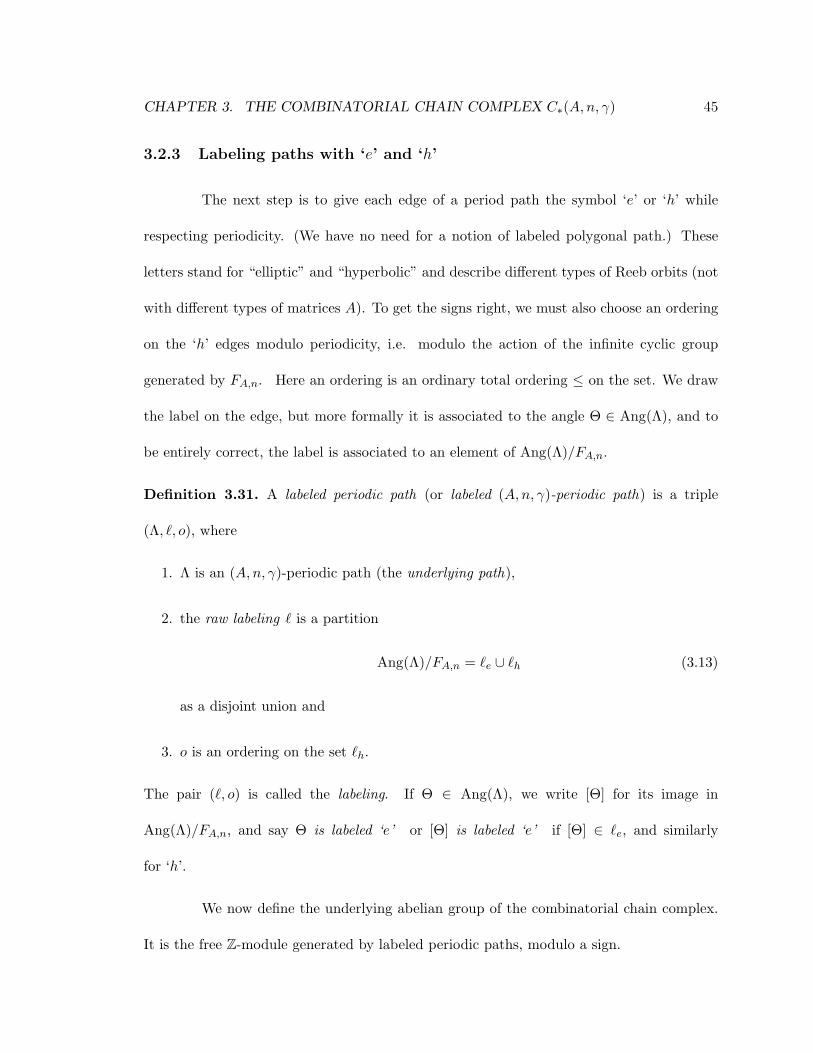
3.2.3 Labeling paths with ‘e’ and ‘h’
The next step is to give each edge of a period path the symbol ‘e’ or ‘h’ while
respecting periodicity. (We have no need for a notion of labeled polygonal path.) These
letters stand for “elliptic” and “hyperbolic” and describe different types of Reeb orbits (not
with different types of matrices A). To get the signs right, we must also choose an ordering
on the ‘h’ edges modulo periodicity, i.e. modulo the action of the infinite cyclic group
generated by FA,n. Here an ordering is an ordinary total ordering ≤ on the set. We draw
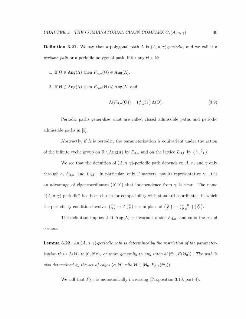
the label on the edge, but more formally it is associated to the angle Θ ∈ Ang(Λ), and to
be entirely correct, the label is associated to an element of Ang(Λ)/FA,n.
Definition 3.31. A labeled periodic path (or labeled (A,n, γ)-periodic path) is a triple
(Λ, `, o), where
1. Λ is an (A,n, γ)-periodic path (the underlying path),
2. the raw labeling ` is a partition
Ang(Λ)/FA,n = `e ∪ `h (3.13)
as a disjoint union and
3. o is an ordering on the set `h.
The pair (`, o) is called the labeling. If Θ ∈ Ang(Λ), we write [Θ] for its image in
Ang(Λ)/FA,n, and say Θ is labeled ‘e’ or [Θ] is labeled ‘e’ if [Θ] ∈ `e, and similarly
for ‘h’.
We now define the underlying abelian group of the combinatorial chain complex.
It is the free Z-module generated by labeled periodic paths, modulo a sign.

CHAPTER 3. THE COMBINATORIAL CHAIN COMPLEX C∗(A,n, γ) 46
Definition 3.32. Let
C∗(A,n, γ) = Z{all labeled (A,n, γ)-periodic paths}/ ∼, (3.14)
where (Λ, `, o) ∼ (Λ, `, o′) if o′ is obtained from o by an even permutation of `h, and
(Λ, `, o) ∼ −(Λ, `, o′) if it is an odd permutation.
Once we introduce δ and a grading, we will be able to call C∗(A,n, γ) a chain
complex.
Definition 3.33. A labeled truncated path is a triple (Λtr, `, o), where Λtr is a truncated
path, the raw labeling ` is a partition
Ang(Λtr) = `e ∪ `h (3.15)
as a disjoint union, and o is an ordering on the set `h. The pair (`, o) is called the labeling.
We say Θ is labeled ‘e’ if Θ ∈ `e, and similarly for ‘h’.
Definition 3.34. Let
Ctr∗ (I) = Z{all truncated paths with Dom(Λtr) = I}/ ∼, (3.16)
where (Λtr, `, o) ∼ (Λtr, `, o′) if o′ is obtained from o by an even permutation of `h, and
(Λtr, `, o) ∼ −(Λtr, `, o′) if o′ is obtained from o by an odd permutation.
We introduce Ctr∗ (I) for the sake of certain subcomplexes of Ctr
∗ (I) in Definition
4.7.
Notation Convention 3.35 (Abusive). We write constp for any constant path at p (polyg-
onal, truncated, periodic; labeled or unlabeled).
CHAPTER 3. THE COMBINATORIAL CHAIN COMPLEX C∗(A,n, γ) 47
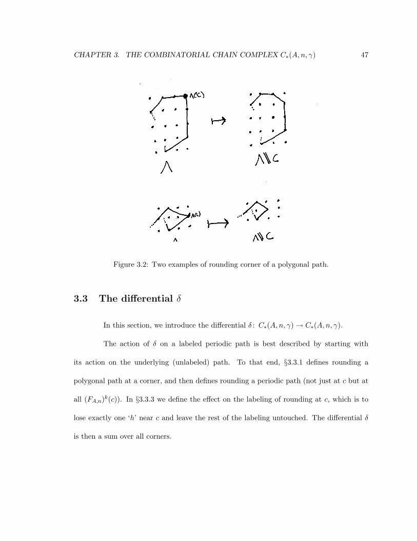
Figure 3.2: Two examples of rounding corner of a polygonal path.
3.3 The differential δ
In this section, we introduce the differential δ : C∗(A,n, γ)→ C∗(A,n, γ).
The action of δ on a labeled periodic path is best described by starting with
its action on the underlying (unlabeled) path. To that end, §3.3.1 defines rounding a
polygonal path at a corner, and then defines rounding a periodic path (not just at c but at
all (FA,n)k(c)). In §3.3.3 we define the effect on the labeling of rounding at c, which is to
lose exactly one ‘h’ near c and leave the rest of the labeling untouched. The differential δ
is then a sum over all corners.
CHAPTER 3. THE COMBINATORIAL CHAIN COMPLEX C∗(A,n, γ) 48
3.3.1 Rounding a corner of a polygonal or truncated path
We introduce the operation of rounding (without periodicity) a corner of a path,
which takes a polygonal path Λ and a proper corner c and produces another polygonal path
denoted Λ\\c. It is helpful to begin the explanation with a picture. Figure 3.2 illustrates
some paths Λ, distinguishes a vertex c for each, and shows the result of rounding Λ at c.
(Someone walking along Λ has cut a corner.) The rounded path Λ\\c “encloses” exactly
one point fewer than Λ. A helpful image (told to me by Michael Hutchings) is to stretch a
rubber band along the path Λ, after putting a nail in each lattice point, nails which hold Λ
taut. Plucking out the nail at Λ(c) causes the rubber band to snap into a new configuration,
Λ\\c. (Small plastic boards, geoboards, with nonremovable nails, illustrate some of this; and
Java applets exist.)
Recall that a corner c is an open interval of angles. We will need to use the closed
interval, c. Figure 3.2 illustrates that rounding at c only affects the two edges adjacent to
c. (The path is unaffected outside c.) The rounded path shortens those edges or removes
them, and inserts any number of new edges.
The formal definition works by deleting Λ(c) from the set of lattice points “en-
closed” by the two edges adjacent to c. The points “enclosed” are those in the triangle with
vertices p = Λ(Θ1 − ε), Λ(c) = Λ(Θ1 + ε) = Λ(Θ2 − ε), and q = Λ(Θ2 + ε). This “triangle”
will be a 2-gon if p = q (though we always have p 6= Λ(c), Λ(c) 6= q).
Definition 3.36. Let Λ be a polygonal path and c = (Θ1,Θ2) a proper corner of Λ. We
define Λ\\c, the result of rounding (without periodicity) Λ at c, as follows:
1. Let p be the beginning of EdgeΛ(Θ1) and q the end of EdgeΛ(Θ2).
CHAPTER 3. THE COMBINATORIAL CHAIN COMPLEX C∗(A,n, γ) 49
2. Let L be the set of points of LA,Γ contained in the convex hull of p, Λ(c), and q.
3. The convex hull of L\{Λ(c)} is some polygon P . Traverse its boundary counterclock-
wise starting at p and ending at q, forming a set E of directed line segments.
(If P is a point, this set E is empty. If P is a 2-gon and p 6= q, E is the edge from p
to q. If P is a 2-gon and p = q, E is an edge from p to the other vertex of p, and an
edge from there to q. )
4. Equip each directed line segment σ ∈ E with an angle Θ, so that the vector from the
beginning of σ to the end is a positive real multiple of (cos Θ, sin Θ) (see Definition 3.15,
Part 1), and resolve the 2πZ ambiguity by requiring Θ ∈ c = [Θ1,Θ2].
5. We have formed a set of pairs (σ,Θ). Let Λ\\c be the union of that set and {(σ,Θ) ∈ Λ | Θ /∈ c}.
(If this construction results in an empty set of edges, let Λ\\c = constp(= constq).)
The polygon P has an edge from q to p (if q 6= p) that is not included in Λ\\c.
Lemma 3.37. For all Θ ∈ c, Λ(Θ) 6= (Λ\\c)(Θ) when both expressions are defined.
Proof. By construction, Λ\\c never touches the vertex Λ(c), at least for Θ ∈ c. (It may, of
course, loop around and reach Λ(c) for some Θ far from c.)
Lemma 3.38. The parameterizations Λ(Θ) and (Λ\\c)(Θ) agree outside c.
Proof. This is true by construction, separately for nonconstant and constant Λ\\c.
Rounding a truncated path Λtr works the same way as rounding a polygonal path.
The term “proper corner” of Λtr rules out a corner at either end of the interval Dom(Λtr).
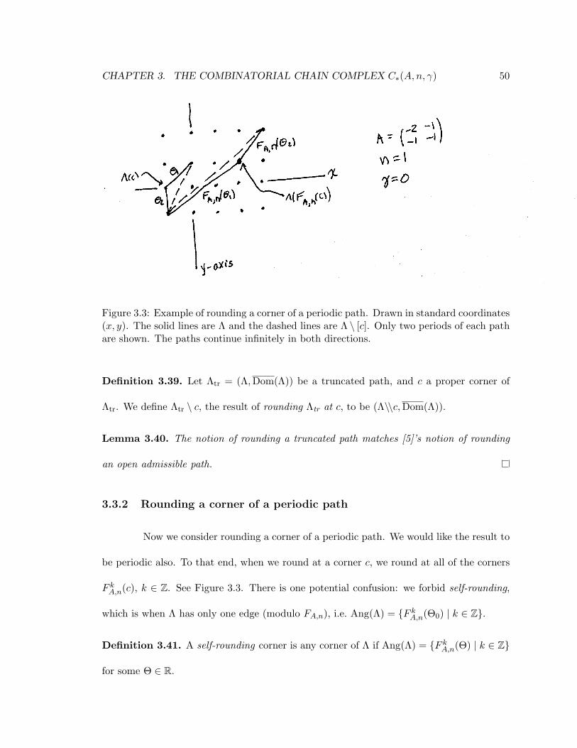
CHAPTER 3. THE COMBINATORIAL CHAIN COMPLEX C∗(A,n, γ) 50
Figure 3.3: Example of rounding a corner of a periodic path. Drawn in standard coordinates(x, y). The solid lines are Λ and the dashed lines are Λ \ [c]. Only two periods of each pathare shown. The paths continue infinitely in both directions.
Definition 3.39. Let Λtr = (Λ,Dom(Λ)) be a truncated path, and c a proper corner of
Λtr. We define Λtr \ c, the result of rounding Λtr at c, to be (Λ\\c,Dom(Λ)).
Lemma 3.40. The notion of rounding a truncated path matches [5]’s notion of rounding
an open admissible path.
3.3.2 Rounding a corner of a periodic path
Now we consider rounding a corner of a periodic path. We would like the result to
be periodic also. To that end, when we round at a corner c, we round at all of the corners
F kA,n(c), k ∈ Z. See Figure 3.3. There is one potential confusion: we forbid self-rounding,
which is when Λ has only one edge (modulo FA,n), i.e. Ang(Λ) = {F kA,n(Θ0) | k ∈ Z}.
Definition 3.41. A self-rounding corner is any corner of Λ if Ang(Λ) = {F kA,n(Θ) | k ∈ Z}
for some Θ ∈ R.
CHAPTER 3. THE COMBINATORIAL CHAIN COMPLEX C∗(A,n, γ) 51
Self-rounding is only an issue if N = 1.
Lemma 3.42. If N > 1, any self-rounding corner is a kink.
Proof. Suppose Ang(Λ) = {F kA,n(Θ) | k ∈ Z}. Since Λ cannot have an edge of the form πk,
Θ ∈ (πk, π(k + 1)) for some k, and FA,n(Θ) ∈ (π(k + N), π(k + N + 1)). In particular,
FA,n(Θ) > π(k + 2) and Θ < π(k + 1) so c = (Θ, FA,n(Θ)) has width greater than π.
Remark 3.43. We forbid self-rounding to obtain a combinatorial chain complex that com-
putes ECH, but in addition the result of self-rounding on a labeled path would be very difficult
to define.
Working with non-self-rounding corners, we may assume that c is not identified
(by periodicity) with the adjacent corner, and the edge before c is not identified with the
edge after.
For a periodic path, a proper corner is a corner that is not a kink (i.e., proper
(Θ1,Θ2) has Θ2 −Θ1 ≥ π). We define corner-mod-periodicity, and build in the conditions
we need.
Definition 3.44. A corner-mod-periodicity of an (A,n, γ)-periodic path Λ is a set
[c] = {F kA,n(c) | k ∈ Z}, (3.17)
where c is a proper corner of Λ that is not a self-rounding corner. We call [c] the corner-
mod-periodicity of c.
We check a well-definedness condition regarding proper corners.
Lemma 3.45. If c is a proper corner of an (A,n, γ)-periodic path Λ, then F kA,n(c) is also
a proper corner.
CHAPTER 3. THE COMBINATORIAL CHAIN COMPLEX C∗(A,n, γ) 52
Proof. The only thing to check is that if c = (Θ1,Θ2) with Θ2 −Θ1 ≤ π, then FA,n(Θ2)−
FA,n(Θ1) ≤ π. This follows from the monotonicity of FA,n (Proposition 3.10, Part 4) once
we show that FA,n(Θ1 + π)− FA,n(Θ1) = π.
The action (denoted(a 00 a−1
)S1) of
(a 00 a−1
)on the circle in R2 sends opposite points
to opposite points, and sends an arc going π around the circle to another such arc. The
lift FA,n of(a 00 a−1
)S1 sends an interval of length π to another such interval, and preserves
orientation. Thus, FA,n(Θ1 + π) = FA,n(Θ1) + π.
Definition 3.46. Let Λ be a periodic path and [c] = {F kA,n(c) | k ∈ Z} a corner-mod-
periodicity. We define the result of rounding (with periodicity) Λ at [c], Λ \ [c], also called
Λ \ c or rounding Λ at [c] or at c, to be the result of simultaneously rounding (without
periodicity) Λ at F kA,n(c) for all k ∈ Z.
(If the result is Ang(Λ \ [c]) = ∅, let Λ \ [c] be the constant path at Λ(Θ) for
Θ /∈⋃F kA,n(c).)
The last proviso enforces what is otherwise automatic, that rounding at [c] only
affects the parameterization inside⋃F kA,n(c). Rounding at [c] = [(Θ1,Θ2)] can only result
in Ang(Λ \ c) = ∅ if we already had Λ(Θ1− ε) = Λ(Θ2 + ε), in which case Λ(Θ) si the same
for any Θ ∈⋃F kA,n(c).
That the infinitely many rounding operations may be performed simultaneously
without interfering with one another follows from Lemma 3.38, and is also illustrated in Fig-
ure 3.3, which illustrates a((−2 −1−1 −1
), 1, 0
)-periodic path Λ with Ang(Λ) = {. . . ,Θ1,Θ2, FA,n(Θ1), FA,n(Θ2), F 2
A,n(Θ1), . . .},
the smallest possible non-self-rounding Ang(Λ)/FA,n. Rounding (without periodicity) at

CHAPTER 3. THE COMBINATORIAL CHAIN COMPLEX C∗(A,n, γ) 53
c = (Θ1,Θ2) affects things before q = Λ((Θ2, FA,n(Θ1))) and rounding (without periodic-
ity) at FA,n(c) affects things after q. The result Λ \ c is again((−2 −1−1 −1
), 1, 0
)-periodic.
As a consequence of our definitions, when we speak of rounding a periodic path,
we always mean rounding it in the sense of periodic paths, and rounding a corner c is really
rounding at the corner-mod-periodicity [c].
Lemma 3.47. The parameterizations Λ(Θ) and (Λ\ c)(Θ) agree outside⋃k∈Z F
kA,n(c).
Definition 3.48. If Λ \ c is defined, and Θ ∈ c, let Λ \Θ = Λ \ c.
An equivalent characterization of Λ \ c, using the notion of “to the left”, is given
in Proposition 3.69.
3.3.3 Losing one ‘h’ from the labeling
We can round a labeled periodic path or labeled truncated path α at a corner c by
rounding the underlying unlabeled path at c and locally (in c) decreasing the number of ‘h’
labels by one, while leaving the labels elsewhere (mod periodicity) unchanged. The result,
δcα, is a signed sum of labeled paths. (All our labeled paths are periodic or truncated.)
The number of ‘h’ labels of Λ near c, i.e. in c, is 0, 1, or 2. (If c = (Θ1,Θ2), then
Λ has edges at Θ1 and Θ2 and nowhere else in c = [Θ1,Θ2].) If that number is zero (i.e., if
we round at a corner between two ‘e’ edges), then δcα = 0.
Since Λ and Λ \ c already agree outside c, or [c] if Λ is periodic, it makes sense
to speak of the labelings agreeing outside c or [c]. (In the periodic case, this means the
labelings agree outside F kA,n(c), k ∈ Z.) Recall that we may write Λ \ c when Λ is periodic,
even though Λ \ [c] is the more elegant description of where we are rounding.
CHAPTER 3. THE COMBINATORIAL CHAIN COMPLEX C∗(A,n, γ) 54
Definition 3.49. Let α = (Λ, `, o) be a labeled periodic path or labeled truncated path
in Ctr∗ (I) or C∗(A,n, γ). Let c be a proper corner of Λ if Λ is truncated, or a proper
non-self-rounding corner of Λ if Λ is periodic. The result δcα of rounding α at c is
δcα =∑`′
±(Λ \ c, `′, o′), (3.18)
where the sum is over all raw labelings `′ of Λ \ c such that
1. In c, `′ has exactly one less ‘h’ than `. (So |`′h ∩ c| = |`h ∩ c| − 1.)
2. The raw labeling `′ agrees with ` outside c if Λ is truncated, or outside [c] =⋃
(FA,n)k(c)
if Λ is periodic.
and where o′ and ± are determined by Sign Convention 3.50.
The sum has one term for each `′ satisfying the two conditions, which may be an
empty sum.
The sign convention involves the order of ‘h’ edges. We may assume ` has at least
one ‘h’ edge in c (otherwise δcα = 0). Assume that the first ‘h’ edge in the ordering is
adjacent to c. This can always be arranged, possibly at the expense of a minus sign, by
changing the order so that the desired ‘h’ edge is the first one. The idea is that this first
‘h’ edge is deleted from the ordering.
Recall that [Θ] is the equivalence class of Θ modulo FA,n, if Λ is periodic.
Sign Convention 3.50. Suppose we have the hypotheses of Definiton 3.49, and an `′
satisfying the conditions given there. If Λ is truncated, let [Θ] = Θ. We may suppose,
choosing if necessary a representative (Λ, `, o) of the equivalence class in C∗ = Z{paths}/ ∼,
that

CHAPTER 3. THE COMBINATORIAL CHAIN COMPLEX C∗(A,n, γ) 55
1. The first ‘h’-labeled angle in the ordering o, which we will call Θh, is an endpoint of
c. (Technically, it is [Θh] that has the first ‘h’ label, and Θh that we require to be an
endpoint of c.)
2. If Θh is the only ‘h’-labeled angle in c, c ∩ `h = {[Θh]}, then o′ is the restriction of
the order o to `′h = `h \ {[Θh]}.
3. If there are two ‘h’-labeled angles in c, c ∩ `h = {[Θh], [Θ2]}, then o′ is the restriction
of the order o to `′h after identifying [Θ2] with the ‘h’-labeled angle of `′h in c, i.e.
identifying [Θ2] with [Θ′] where c ∩ `′h = {[Θ′]}.
Then (see Figure 3.4) the term appearing in the sum (3.18) is
+(Λ \ c, `′, o′) (3.19)
if Θh is the beginning of c (c = (Θh,Θ2)), and
−(Λ \ c, `′, o′) (3.20)
if Θh is the end of c (c = (Θ2,Θh)).
Once o satisfies Part 1 of Sign Convention 3.50, o′ is determined by Part 2 or 3.
We have to make a choice to get o to satisfy Part 1, and in particular, we may have to
choose which of two ‘h’ edges to call Θh, but the choice does not matter:
Lemma 3.51. Under the hypotheses of Definition 3.49, δcα is well-defined as a element of
Ctr∗ (I) or C∗(A,n, γ).
Proof. In computing δc, we choose a representative ±(Λ, `, o) of an equivalence class in C∗,
and in particular, if there are two ‘h’ labels in c, we choose one to be first in o. We may
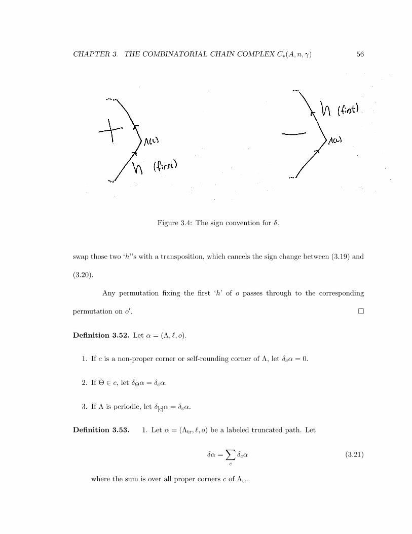
CHAPTER 3. THE COMBINATORIAL CHAIN COMPLEX C∗(A,n, γ) 56
Figure 3.4: The sign convention for δ.
swap those two ‘h’’s with a transposition, which cancels the sign change between (3.19) and
(3.20).
Any permutation fixing the first ‘h’ of o passes through to the corresponding
permutation on o′.
Definition 3.52. Let α = (Λ, `, o).
1. If c is a non-proper corner or self-rounding corner of Λ, let δcα = 0.
2. If Θ ∈ c, let δΘα = δcα.
3. If Λ is periodic, let δ[c]α = δcα.
Definition 3.53. 1. Let α = (Λtr, `, o) be a labeled truncated path. Let
δα =∑c
δcα (3.21)
where the sum is over all proper corners c of Λtr.

CHAPTER 3. THE COMBINATORIAL CHAIN COMPLEX C∗(A,n, γ) 57
2. Let α = (Λ, `, o) be a labeled (A,n, γ)-periodic path. Let
δα =∑[c]
δ[c]α, (3.22)
where the sum is over all corners-mod-periodicity [c] of Λ.
In other words, if Λ is periodic, we have one summand δcα for the entire family
{F kA,n(c)}k∈Z.
We now give two examples we will be using often.
Example 3.54. If Λ is a truncated or periodic path, we define two cycles EΛ, HΛ in Ctr∗ (I)
or C∗(A,n, γ) as follows:
1. EΛ is the labeled path consisting of the path Λ with edges labeled ‘e’.
2. HΛ is a sum of labeled paths: It is the sum over all ways to label one edge of Λ ‘h’
and all the others ‘e’. The sum is empty (HΛ = 0) if and only if Λ is constant.
In both cases, the ordering o is trivial.
Proof. We see δEΛ = 0 because it cannot lose one ‘h’. We see δHΛ = 0 because, if
c = (Θ1,Θ2) (we may assume c is not a self-rounding corner), any contribution to δcHΛ
from the term of HΛ where Θ1 is labeled ‘h’ cancels the contribution from the term where
Θ2 is labeled ‘h’.
Definition 3.55. The number of ‘h’ labels, i.e. the number of elements of `h, is denoted
#h(`).
Proposition 3.56. The differential on labeled truncated paths is equivalent to the differ-
ential on open admissible paths from [5, Definitions 3.4, 3.5]; the isomorphism is given by
reversing the ordering of ‘h’ labels and multiplying (Λtr, `, o) by (−1)#h(`).
CHAPTER 3. THE COMBINATORIAL CHAIN COMPLEX C∗(A,n, γ) 58
Proof. The definitions in [5] correspond to the ones here except for the sign convention
there, which is + if the last ‘h’ in the ordering is just after c and − if it is before.
Corollary 3.57 (by §3.2 of [5]). On Ctr∗ (I), we have δ2 = 0.
Thus (Ctr∗ (I), δ) is a chain complex. We have not given it a grading, but a relative
grading is given in [5, §3.1.5].
Proposition 3.58. On C∗(A,n, γ), we have δ2 = 0.
Proof. The proof in [5, §3.2] carries over to C∗(A,n, γ) for paths Λ with at least three edges
(mod periodicity), because whenever we consider δbδaα (α = (Λ, `, o), a a corner of Λ, b a
corner of Λ \ c), there exists Θ outside [a] and [b], and all the action can be understood
on the truncated path Λ|[Θ, FA,n(Θ)]. (By the arguments in [5], either b is “created” by
rounding at a (b ⊆ a) or else b comes from a corner of Λ, possible a corner smaller than
the interval b, expanded by rounding at a. In either case, such Θ must exist. We choose Θ
outside Ang(Λ).)
If Λ has at most one edge, we already have δα = 0. (We use “no self-rounding”–
see Definition 3.44 and Definition 3.53.) So, assume Λ has two edges: a = (Θ1,Θ2) and
Ang(Λ) = {. . . ,Θ1,Θ2, FA,n(Θ1), . . .}. We may assume a is not a kink. Both edges of Λ
participate in rounding at a and all edges of Λ \ a receive labels by the rules for δa. Thus
δaα is one of the cycles EΛ\a or HΛ\a, so δδaα = 0.
Thus (C∗(A,n, γ), δ) is a chain complex. We will give it a grading in §3.4.

CHAPTER 3. THE COMBINATORIAL CHAIN COMPLEX C∗(A,n, γ) 59
3.4 The index I((Λ, `, o)) gives a grading on C∗(A, n, γ)
At this point in building our chain complex C∗(A,n, γ), we have a group and a
differential δ on it. We need a grading. In this section, we will define the index I(α) of a
labeled periodic path α, allowing us to write the group as⊕
iCi(A,n, γ). There is only a
relative index in general: I(α) ∈ Z with Z a torsor over Z, so I(α1) − I(α2) ∈ Z. When
Γ = 0, we choose a particular isomorphism Z ∼= Z by requiring I(const0) = 0.
The formula for the relative index, stated precisely in Definitions 3.63 and 3.64 as
well as Lemma-Definition 3.65, is essentially
I((Λ, `, o)) = 2 Size(Λ)−#h(`), (3.23)
where #h is the number of ‘h’ labels, mod periodicity; and Size(Λ) is something like the
number of lattice points enclosed by Λ, but only defined up to adding a constant. The
number of lattice points enclosed by Λ \ c is one less than the number enclosed by Λ, which
will mean δ has degree −1 (Proposition 3.66).
We take an axiomatic approach, showing that there is essentially only one function
Size.
Definition 3.59. A relative size function is a map
Size : {(A,n, γ)-periodic paths} → R (3.24)
such that
Size(Λ \ c) = Size(Λ)− 1 (3.25)
where c is a proper corner-mod-periodicity of the (A,n, γ)-periodic path Λ.
CHAPTER 3. THE COMBINATORIAL CHAIN COMPLEX C∗(A,n, γ) 60
A relative size function is, in effect, an embedding of the torsor Z into R. We say
R for generality, though we never need anything worse than Q.
Proposition 3.60. Given A, n, and γ, there exists a relative size function, and it is unique
up to adding a constant.
We will prove Proposition 3.60 in §3.6.
Example 3.61. Recall (though we normally work with just hyperbolic A and −1) that
(1, 1, 0)-periodic paths are just convex polygons (with vertices in LA,Γ). Let Size(Λ) be the
number of points (nonstrictly) enclosed by Λ. This quantity is well-defined.
Example 3.62. A (−1, 1, γ)-periodic path Λ is a convex polygon with (X,Y ) 7→ (−X,−Y )
symmetry. One period is Λ|[0, π], and the polygon is Λ|[0, 2π]. Let Size(Λ) be one half of
the number of points (nonstrictly) enclosed by the polygon.
When A is hyperbolic it is harder to define the number of points enclosed.
For the following definition, we write I(α, α′) for I(α)− I(α′), since we cannot yet
define I(α).
Definition 3.63. If α = (Λ, `, o) and α′ = (Λ′, `′, o′) are labeled (A,n, γ)-periodic paths
and Size is a relative size function, let
I(α, α′) = [2 Size(Λ)−#h(`)]− [2 Size(Λ′)−#h(`′)], (3.26)
where #h(`) is the cardinality of `h.
We see that I(α, α′) is the same for any relative size function.
When Γ 6= 0, we live with the ambiguity in I(α). When Γ = 0, we use the
expression Size(Λ)− Size(const0) to obtain I(const0) = 0.
CHAPTER 3. THE COMBINATORIAL CHAIN COMPLEX C∗(A,n, γ) 61
Definition 3.64. If α is a labeled (A,n, 0)-periodic path, its index (or absolute index ) is
I(α) = 2(Size(Λ)− Size(const0))−#h(`). (3.27)
Lemma-Definition 3.65. For any Γ, we may define a Z-torsor Z and the relative index,
I : {Labeled (A,n, γ)-periodic paths} → Z, (3.28)
such that I(α, α′) = I(α)− I(α′).
If Γ = 0, Z is naturally Z, and I is the absolute index.
Proof. The claim is straightforward but hard to make moderately formal. To be absurdly
formal, let Z be the set
{− Size | Size is a Z-valued relative size function}, (3.29)
and let I(Λ, `, o) be the element −Size such that 2 Size(Λ)−#h(`) = 0.
Proposition 3.66. If α is a labeled (A,n, γ)-periodic path, I(δα) = I(α)− 1.
Proof. We see that I(α, δα) = 1 using the definition of I, the fact that δ decreases Size by
1 (by the definition of relative size function), and decreases #h by 1 (by the definition of
δ).
3.5 The partial order ≤ (“to the left”) on periodic paths
In the current section, we define a partial order on periodic paths. The relation
is denoted Λ ≤ Λ′ and called to the left, a term motivated by the point of view of bugs
crawling along the paths. Another intuition for Λ ≤ Λ′ is that Λ is smaller than Λ′. For
instance, Λ will have smaller Size than Λ′.
CHAPTER 3. THE COMBINATORIAL CHAIN COMPLEX C∗(A,n, γ) 62
Definition 3.67. 1. Given (A,n, γ)-periodic paths Λ,Λ′, we say Λ ≤ Λ′ if
det(Λ′(Θ)− Λ(Θ), ~Θ) ≥ 0 (3.30)
for all Θ such that neither Λ nor Λ′ has an edge at Θ. We say Λ is to the left of Λ′.
2. Given truncated paths Λ,Λ′ with Dom(Λ) = Dom(Λ′), we say Λ ≤ Λ′, or Λ is to
the left of Λ′, if (3.30) holds for all Θ where it makes sense, i.e., Θ ∈ Dom(Λ) with
Θ /∈ Ang(Λ) ∪Ang(Λ′).
3. We may compare truncated paths with different domains, or a truncated path with a
periodic path, by restricting domains in the obvious way. For periodic paths specifi-
cally, saying Λ ≤ Λ′ implies that Λ and Λ′ have the same (A,n, γ).
In [5], truncated paths compared with ≤ are required to be defined on the same
interval, and also required to have matching endpoints, i.e., Λ(Θi) = Λ′(Θi), i = 1, 2, where
Λ and Λ′ are defined on [Θ1,Θ2]. We do not build either condition into the definition.
The restriction that Λ and Λ′ have no edge at Θ is not really necessary because
the expression det(Λ′(Θ)− Λ(Θ), ~Θ) extends to a continuous function on all Θ.
We see, for (A,n, γ)-periodic Λ and Λ′, that Λ ≤ Λ′ iff Λ|[0, Nπ] ≤ Λ′|[0, Nπ] iff
Λ|I = Λ′|I for all intervals I.
Proposition 3.68. The relation ≤ on (A,n, γ)-periodic paths is a partial order. The rela-
tion ≤ on truncated paths defined on a given interval is a partial order.
Proof. We see that Λ ≤ Λ. If
Λ ≤ Λ′ ≤ Λ, (3.31)

CHAPTER 3. THE COMBINATORIAL CHAIN COMPLEX C∗(A,n, γ) 63
then det(Λ′(Θ) − Λ(Θ), ~Θ) = 0. The function of Θ, Λ′(Θ) − Λ(Θ), is piecewise constant,
and each value it takes is a vector parallel to multiple Θ’s (with linearly independent ~Θ’s).
Thus, Λ = Λ′.
For transitivity, add determinants: det(Λ′′(Θ)−Λ′(Θ), ~Θ)+det(Λ′(Θ)−Λ(Θ), ~Θ) ≥
0 so Λ ≤ Λ′′.
Proposition 3.69 (Alternate characterization of rounding a corner). If Λ is a periodic or
truncated path and c is a proper corner of Λ, then:
1. Λ\c ≤ Λ.
2. (Λ \ c)(Θ) disagrees with Λ(Θ) at every Θ ∈ c for which both expressions are defined.
3. If Λ′ ≤ Λ is a path (periodic if Λ is periodic, or truncated and defined on the same
interval as Λ if Λ is truncated) with Λ′(Θ) 6= Λ(Θ) for at least one Θ ∈ c, then
Λ′ ≤ Λ\c.
Proof. Part 2 for periodic and truncated paths follows from the corresponding statement
for polygonal paths, Lemma 3.37.
Parts 1 and 3 are essentially the same as [5, Proposition 2.10], and the proof given
there works in this situation. Note that the proof in [5] does not use the requirement
imposed there, that endpoints match. Note also (Lemma 3.47) that for periodic paths, Λ
and Λ \ c agree outside⋃k∈Z F
kA,n(c), reducing the problem to an operation local in Θ,
taking place on each F kA,n(c) separately.
CHAPTER 3. THE COMBINATORIAL CHAIN COMPLEX C∗(A,n, γ) 64
It will turn out that for periodic paths (and for truncated paths with more dis-
claimers), Λ ≤ Λ′ if and only if Λ may be obtained from Λ′ by a sequence of roundings.
(See the proof of Lemma 3.77, or [5, Proposition 2.13].)
Lemma 3.70. 1. If Λ ≤ Λ′ and c is a kink of Λ′, then Λ(Θ) = Λ′(Θ) for all Θ ∈
c. (We require the domain of Λ′ to be strictly wider than c: If c = (Θ1,Θ2) then
(Θ1 − ε,Θ2 + ε) ⊂ Dom(Λ′) for some ε > 0.)
2. If Λtr ≤ Λ′tr are truncated paths, both defined on [Θ1,Θ2] with matching endpoints,
and c is a corner of Λ′tr containing Θ1 or Θ2, then Λtr(Θ) = Λ′tr(Θ) for all Θ ∈ c.
Proof. 1. This is [5, Proposition 2.12]. The proof given there does not use the stronger
characterization of ≤ in that paper. The statement is local in Θ, so it follows for
periodic paths as well as truncated ones.
2. A truncated path Λtr (respectively Λ′tr) has an underlying polygonal path Λ (resp.
Λ′) defined on all of R, with Λ(Θ) = Λtr(Θ1) for Θ ≤ Θ1 and Λ(Θ) = Λtr(Θ2) for
Θ ≥ Θ2. We may apply Part 1 to the corner of Λ′ containing Θ1 or Θ2.
Lemma 3.71. There are only finitely many (A,n, γ)-periodic paths to the left of a given
(A,n, γ)-periodic path.
Proof. We will show that if Λ is fixed and λ ≤ Λ, the points of λ|[0, Nπ] must lie in a
bounded rectangular region, depending on Λ. Since LA,Γ is discrete, it has only finitely
many points in that region, so there are finitely many possible vertices of λ, finitely many
possible angles Θ ∈ Ang(λ), finitely many possible sets Ang(Λ), and finitely many paths λ.

CHAPTER 3. THE COMBINATORIAL CHAIN COMPLEX C∗(A,n, γ) 65
The path λ can only travel up (+Y direction) while Θ ∈ [0, π]. Applying the
definition of ≤ at Θ = 0, Θ = π shows that
Y (Λ(0)) ≤ Y (λ(0)), Y (λ(π)) ≤ Y (Λ(π)), (3.32)
with Y (λ(Θ)) (Θ ∈ [0, π]) in between,
Y (λ(Θ)) ∈ [Y (Λ(0)), Y (Λ(π))]. (3.33)
Similar reasoning bounds Y on each λ|[kπ, (k + 1)π], and therefore on λ|[0, Nπ]. For the
X-coordinate, use enough intervals of the form [kπ+π/2, (k+ 1)π+π/2]. Thus λ(Θ) must
lie in some bounded rectangle for Θ ∈ [0, Nπ], completing the proof.
3.6 The proof of Proposition 3.60
Recall that the lattice LA,Γ, which looks messy in our usual (X,Y )-coordinates,
looks like Z2 in (x, y)-coordinates.
Definition 3.72. Given a polygonal path Λ and Θ ∈ Ang(Λ), letting p be the beginning and
q the end of EdgeΛ(Θ), define the multiplicity Mult(Λ,Θ) to be gcd(x(q)−x(p), y(q)−y(p)).
The following definition integrates an area form over what is essentially Λ|[Θ0, FA,n(Θ0)],
but because of our odd (piecewise-constant) parameterization of Λ, we write out∫
Λ... as an
integral over each edge of Λ. Each edge (we recall) carries an orientation.
Lemma-Definition 3.73. For any Θ0 ∈ R \Ang(Λ), let
SizeR (Λ) =∑
Θ∈Ang(Λ)Θ0≤Θ<FA,n(Θ0)
∫EdgeΛ(Θ)
X dY +12
∑Θ∈Ang(Λ)
Θ0≤Θ<FA,n(Θ0)
Mult(Λ,Θ). (3.34)
The choice of Θ0 does not affect SizeR (Λ), and SizeR is a relative size function.

CHAPTER 3. THE COMBINATORIAL CHAIN COMPLEX C∗(A,n, γ) 66
This result, which we will prove shortly, establishes the existence portion of Propo-
sition 3.60.
Incidentally, this size function has the pleasing property that SizeR (const0) = 0
when Γ = 0. It is one of at least two (inequivalent) ways to extend the idea Size(const0) = 0
to the case 0 /∈ LA,Γ, i.e. Γ 6= 0.
Remark 3.74. We could obtain the same relative size function as in (3.34) by integrating
any 1-form ω invariant under the pullback(a 00 a−1
)∗ω = ω and satisfying dω = dX ∧ dY .
The value of that integral may also be defined as the area (with signs and multiplicity)
enclosed by the following path: Λ|[Θ0, FA,n(Θ0)], followed by a path τ to 0, followed by(a 00 a−1
)−1τ traversed backwards to Λ(Θ0).
Proof of Lemma-Definition 3.73. We first show that SizeR (Λ) is independent of Θ0. The
integrals and multiplicities are both applied to EdgeΛ(Θ) for Θ ∈ Ang(Λ)∩ [Θ0, FA,n(Θ0)).
So it is sufficient to show that removing a Θ from that set and adding FA,n(Θ) does not
change the result.
The integral is unchanged because X dY is(a 00 a−1
)-invariant. The multiplicity
is unchanged because, in Z2, gcd(a, b) is A-invariant (A ∈ SL2(Z)). Thus, SizeR (Λ) is
independent of Θ0.
It remains to show that SizeR (Λ \ c) = SizeR (Λ) − 1. Write c = (Θ1,Θ2); we may
assume [Θ1,Θ2] ⊂ (Θ0, FA,n(Θ0)). The only differences between Λ and Λ \ c occur on
[Θ1,Θ2], so the issue is a local one, and the proof in [5, Def. 3.3, Lemma 3.9] (using Pick’s
formula) applies here.
The following lemma, that large rectangles contain many lattice points, is much
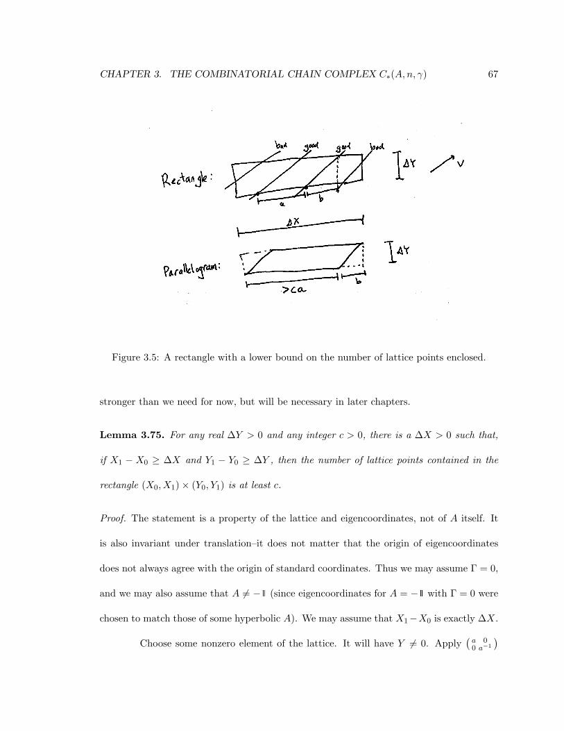
CHAPTER 3. THE COMBINATORIAL CHAIN COMPLEX C∗(A,n, γ) 67
Figure 3.5: A rectangle with a lower bound on the number of lattice points enclosed.
stronger than we need for now, but will be necessary in later chapters.
Lemma 3.75. For any real ∆Y > 0 and any integer c > 0, there is a ∆X > 0 such that,
if X1 − X0 ≥ ∆X and Y1 − Y0 ≥ ∆Y , then the number of lattice points contained in the
rectangle (X0, X1)× (Y0, Y1) is at least c.
Proof. The statement is a property of the lattice and eigencoordinates, not of A itself. It
is also invariant under translation–it does not matter that the origin of eigencoordinates
does not always agree with the origin of standard coordinates. Thus we may assume Γ = 0,
and we may also assume that A 6= −1 (since eigencoordinates for A = −1 with Γ = 0 were
chosen to match those of some hyperbolic A). We may assume that X1−X0 is exactly ∆X.
Choose some nonzero element of the lattice. It will have Y 6= 0. Apply(a 00 a−1
)
CHAPTER 3. THE COMBINATORIAL CHAIN COMPLEX C∗(A,n, γ) 68
repeatedly to shrink its Y -coordinate until we obtain a new point with Y -coordinate is less
than ∆Y . Let v be the vector from origin to the new point. Consider the family of all lines
parallel to v that go through lattice points. Such a line, if it passes through the top and
bottom edge of our rectangle, must contain at least one lattice point in the rectangle. See
Figure 3.5. Let a be the X-distance between adjacent lines in the family (i.e., translating
a line by (a, 0) yields the next line), and let b be such that (b,∆Y ) is parallel to v. (The
lines cannot be parallel to either axis, so we may assume a, b > 0.) Choose
∆X > ca+ b (3.35)
which ensures that the rectangle contains a parallelogram (see the figure) which meets at
least c of the lines, each with at least one lattice point, proving the claim.
Lemma 3.76. For any two (A,n, γ)-periodic paths Λ0 and Λ, there exists an (A,n, γ)-
periodic path Λ′ so big that Λ0 ≤ Λ′ and Λ ≤ Λ′.
Proof. Construct Λ′ by choosing a periodic sequence of points “very far” to the northeast,
northwest, etc. of Λ and Λ0, and connecting them, proceeding counterclockwise.
Lemma 3.77. For any two (A,n, γ)-periodic paths Λ0 and Λ, there exists a sequence
Λ0,Λ1,Λ2, . . . ,Λm = Λ (3.36)
such that for each k = 0, . . . ,m − 1, one of Λk,Λk+1 is obtained by rounding some corner
of the other.
Proof. Given Λ0 and Λ, let Λ′ be as in Lemma 3.76. We will show that there is a sequence
of roundings from Λ′ to Λ (each path in a sequence being obtained by rounding the previous
CHAPTER 3. THE COMBINATORIAL CHAIN COMPLEX C∗(A,n, γ) 69
path at some corner). A similar argument will show there is a sequence of roundings from
Λ′ to Λ0. We may then produce a sequence (3.36) from Λ0 to Λ by joining the two sequences
just constructed.
Suppose Λ ≤ Λ′ and Λ 6= Λ′. The two paths must disagree at at least one Θ, which
lies in some corner c of Λ′. By Lemma 3.70, Λ and Λ′ agree on kinks, so c is not a kink.
Let Λ′1 = Λ′ \ c. We have Λ ≤ Λ′1 ≤ Λ′ by Proposition 3.69.
We may continue in this way: If Λ′1 6= Λ, we may round some corner of Λ′1,
obtaining a new path Λ′2 with Λ ≤ Λ′2 ≤ Λ′1 ≤ Λ′. This process can only terminate when
we obtain a path equal to Λ. We must show it terminates after finitely many steps.
Each path in the sequence is to the left of the one before, so by transitivity of ≤
(Proposition 3.68), each path in the sequence is to the left of the original Λ′. We know
there are only finitely many paths to the left of Λ′ (Lemma 3.71), so provided each term of
the sequence is distinct, the sequence must terminate after finitely many steps, and we are
done. But Λ′i+1 ≤ Λ′i, and Λ′i+1 6= Λ′i. Since ≤ is a partial order, each term is distinct.
Remark 3.78. The symplectic action of a periodic path can be seen as the real reason the
sequence of Λ′i’s terminates in the proof of Lemma 3.77. The symplectic action of a closed
Reeb orbit is the integral of the contact form along the orbit. (See Appendix A for the
correspondence between a periodic path and a collection of Reeb orbits.) Symplectic action
must decrease under rounding, and the set of possible symplectic actions is discrete.
Proof of Proposition 3.60. If remains to show the uniqueness portion of the Proposition.
Let Size be a relative size function. Pick some path Λ0 and let ζ = Size(Λ0) − SizeR (Λ0).
We have Size(Λ) = SizeR (Λ) + ζ for all (A,n, γ)-periodic paths Λ, because Size and SizeR

CHAPTER 3. THE COMBINATORIAL CHAIN COMPLEX C∗(A,n, γ) 70
increase or decrease together as we proceed along the sequence of Lemma 3.77
71
Chapter 4
Boxes and strips define
subcomplexes of C∗(A, n, γ)
Assumption 4.1. Let A ∈ SL2(Z) be hyperbolic or −1, let n be a positive integer, and
let Γ ∈ Z2/ Im(1−A) with γ ∈ Γ.
In this chapter, we introduce two kinds of subcomplex of C∗(A,n, γ), those induced
by boxes and those induced by strips. Boxes and strips are more rectilinear analogues of
periodic paths. Boxes have edges parallel to the X- and Y -axes, the axes of the eigencoor-
dinate system. (The intermediate step in defining boxes is off-lattice periodic paths in §4.1,
paths with vertices allowed to be anywhere in R2.) Strips have infinitely long edges parallel
to the X-axis. The name “box” is intended to suggest a rectangular region in the plane,
and “strip” is intended to suggest an infinitely long rectangle of the form R× [Y0, Y1], but
boxes and strips are slightly more complicated. A box or strip B gives rise to a family
of actual rectangles and infinitely long rectangles, denoted �B,kπ/2, respecting periodicity,

CHAPTER 4. BOXES AND STRIPS DEFINE SUBCOMPLEXES OF C∗(A,n, γ) 72
and we have Λ ≤ B if and only if Λ(kπ/2) ∈ �B,kπ/2 for all k ∈ Z.
The subcomplexes we need are generated by labeled paths to the left of a box
or strip. The main result is that we may use the homologies of boxes to recover the
combinatorial homology H∗(A,n, γ) by a direct limit.
See Propositions 4.18 and 4.19 for details.
The method of Chapter 5 allows us to compute H∗(B) for B a box or strip. Strips
are more useful than boxes, and we will show in Chapter 6 (using boxes in the proof) that
H∗(B) ∼= H∗(A,n, γ) for a strip B.
We introduce off-lattice polygonal paths in §4.1. We define relations ≤Θ and
<Θ , essentially the relation ≤ from §3.5 considered at one Θ, and prove a few lemmas in
§4.2. In §4.3, we define the chain complex generated by periodic paths to the left of a given
off-lattice periodic path, a definition we will need for the case that the off-lattice path is
a box. We also introduce the chain complex generated by truncated paths to the left of a
given truncated path (with matching endpoints), and recall its homology from [5], which
we will need in subsequent chapters. In §4.4, we define boxes and strips, including the chain
complex of a strip, and characterize periodic paths to the left of a box or strip in terms of
≤Θ , and also in terms of �B,Θ. We then prove results about direct limits of boxes.
The concepts of this chapter are a mild generalization of [5, especially §3.1.5].
4.1 Off-lattice paths
Recall that the term polygonal path implies that the vertices lie in the lattice LA,Γ.
Definition 4.2. An off-lattice polygonal path is defined by deleting from the definition of
CHAPTER 4. BOXES AND STRIPS DEFINE SUBCOMPLEXES OF C∗(A,n, γ) 73
polygonal path (Definitions 3.15 and 3.16) the requirement that vertices lie in the lattice
LA,Γ. Instead, we allow vertices of the path to be arbitrary points in the plane. We
carry over every definition from §3.2.1 and §3.2.2 concerning polygonal paths, including the
definition of (A,n, γ)-periodic path, as well as Definition 3.67 of ≤.
Thus, a polygonal path is a kind of off-lattice polygonal path.
Every result of §3.2.1 and §3.2.2 carries over to off-lattice paths, except for the
claims about the relation to the terminology of [5]. (Additionally, though the fact was only
mentioned in passing, polygonal paths have edges only at certain Θ, constrained by the
lattice LA,Γ; off-lattice paths are not thus constrained.) We cannot round a corner of an off-
lattice path. We still have the results on ≤ not dependent on rounding: Proposition 3.68 (≤
is a partial order), and Lemma 3.70 (Λ ≤ Λ′ agrees with Λ′ at a kink of Λ′). Lemma 3.71 can
be generalized to assert that there are finitely many polygonal paths (i.e., lattice polygonal
paths) to the left of a given off-lattice polygonal path.
We are interested in two kinds of off-lattice periodic paths: periodic paths, and
boxes, to be defined later.
4.2 Comparing points and paths with ≤Θ
Recall that the ordering ≤, originally defined on polygonal paths and now gener-
alized to off-lattice polygonal paths, is: Λ ≤ Λ′ if and only if
det(Λ′(Θ)− Λ(Θ), ~Θ) ≥ 0 (4.1)
for all Θ for which Λ′(Θ) and Λ(Θ) are defined. We will often need to compare two points
with respect to some fixed Θ or compare a point and a path, so this section defines a family

CHAPTER 4. BOXES AND STRIPS DEFINE SUBCOMPLEXES OF C∗(A,n, γ) 74
≤Θ of relations using (4.1).
Recall that the set of all angles at which Λ has an edge is denoted Ang(Λ), and
EdgeΛ(Θ) is the edge Λ has at Θ, i.e. the one of the directed line segments out of which Λ
is built.
Definition 4.3. Suppose p and q are points in R2, Θ ∈ R, and Λ and Λ′ are off-lattice
periodic paths, or off-lattice truncated paths defined on an interval including Θ. Define:
1. p ≤Θ q if det(q − p, ~Θ) ≥ 0.
2. p <Θ q if det(q − p, ~Θ) > 0.
3. p ≤Θ Λ if p ≤Θ Λ(Θ), assuming Λ(Θ) is defined; if not, replace Λ(Θ) by some point
r ∈ EdgeΛ(Θ) (it does not matter which point we choose), so p ≤Θ Λ if p ≤Θ r.
4. Λ′ ≤Θ Λ if Λ′(Θ) ≤Θ Λ(Θ), assuming Λ′(Θ),Λ(Θ) are defined; if not, replace
whichever expressions are not defined by a choice of point on the appropriate edge,
as in Part 3, above.
5. p <Θ Λ if p <Θ Λ(Θ), and Λ′ <Θ Λ if Λ′(Θ) <Θ Λ(Θ), with the same disclaimers
as above if Θ is an edge of Λ or Λ′.
We now have a relation ≤ on paths, and relations ≤Θ and <Θ on points and
paths. We do not write “Λ < Λ′”.
For each Θ ∈ R, the relation ≤Θ satisfies all forms of the transitivity property
that make sense.
A truncated path defined on [−π/2, π/2] has an overall motion in the +X direction,
so Λ(−π/2) ≤π/2 Λ(π/2). We generalize this fact.
CHAPTER 4. BOXES AND STRIPS DEFINE SUBCOMPLEXES OF C∗(A,n, γ) 75
Lemma 4.4. If Λ is an off-lattice periodic or truncated path, and Θ,Θ′ ∈ Dom(Λ) with
|Θ′ −Θ| ≤ π, then Λ(Θ′) ≤Θ Λ(Θ).
Proof. If Θ′ ∈ [Θ−π,Θ], then each edge of Λ takes a step in some direction in that interval,
which carries it rightwards, from the point of view of ≤Θ . Similar reasoning applies to
[Θ,Θ + π].
Lemma 4.5. If Λ is periodic and to the left of const0, then Λ = const0. If Λtr is a truncated
path, to the left of constp, and with both endpoints at p, then Λtr = constp.
Proof. For Λ periodic, apply Lemma 3.70, to show that Λ must agree with const0 on its
kink R. For Λtr truncated, let Λ be the “underlying” polygonal path defined on R (from
the definition of truncated path). We still have Λ ≤ constp so Λ = constp.
4.3 Chain complexes of paths to the left of a fixed path
Since Λ\c ≤ Λ, the set of periodic paths Λ to the left of a given off-lattice periodic
path Λ′ is closed under rounding corners. Therefore, the subgroup of C∗(A,n, γ) generated
by (Λ, `, o) with Λ ≤ Λ′ is a subcomplex.
Definition 4.6. Given an off-lattice periodic path Λ′, let C∗(Λ′), or C∗(A,n, γ; Λ′), denote
the subcomplex of C∗(A,n, γ) generated by (Λ, `, o) with Λ ≤ Λ′.
We will be very interested in certain subcomplexes of the form just described,
namely the case where Λ′ is a box, which we are now ready to define. The case that Λ′ is a
(lattice) periodic path is the one considered in [5]. We have introduced off-lattice paths not
CHAPTER 4. BOXES AND STRIPS DEFINE SUBCOMPLEXES OF C∗(A,n, γ) 76
to get subcomplexes unobtainable from lattice paths, but rather to provide more convenient
descriptions of some of those subcomplexes.
Now we turn to complexes involving truncated paths. We only use lattice truncated
paths.
Definition 4.7. Given a truncated path Λtr defined on an interval I, let C∗(Λtr) denote
the subgroup of Ctr∗ (I) generated by (Λ′tr, `, o) with Λ′tr ≤ Λtr, where we require Λ′tr,Λtr to
have the same domain and matching endpoints.
The subgroup C∗(Λtr) is a subcomplex. We need the homology of the subcomplex
in the case where I has width π. We especially need it for intervals of the form [kπ/2, kπ/2+
π], but we may easily state it for all [Θ0,Θ0 + π], taking advantage of our convention that
a truncated path may not have an edge at an angle forming an endpoint of its domain.
Proposition 4.8. Suppose Λtr is defined on I = [Θ0,Θ0 +π] for some Θ0 ∈ R. If Λtr is not
constant, then H∗(Λtr) ∼= Z2, generated by EΛtr and HΛtr. If Λtr is constant, H∗(Λtr) ∼= Z,
generated by EΛtr.
In either case, we may say that H∗(Λtr) is generated by EΛtr and HΛtr , since
Hconstp = 0.
Proof. If Λtr = constp, the only path that can appear in C∗(Λtr) is constp, and the only
way to label it is Econstp . We have δ = 0 and H∗(constp) is as claimed.
If Λtr is not constant, the result follows once we satisfy the hypotheses of [5, Propo-
sition 5.6], which are that Λtr has distinct endpoints, and is convex : “it is parametrized by
an interval of length ≤ 2π and it traverses a subset of the boundary of a convex polygon,

CHAPTER 4. BOXES AND STRIPS DEFINE SUBCOMPLEXES OF C∗(A,n, γ) 77
possibly a 2-gon.” The convex polygon is made by joining to Λtr an edge from Λtr(Θ0 + π)
to Λtr(Θ0). Each vertex of Λtr is to the left in the sense of <Θ0 compared to the previous
vertex. Thus, Λtr(Θ0 + π) <Θ0 Λtr(Θ0) (and in particular these points are distinct) and
the extra edge can be given an angle in (Θ0 + π,Θ0 + 2π), making a convex polygon.
4.4 Boxes and strips
4.4.1 Boxes
A box is essentially an off-lattice periodic path with edges parallel to the X and
Y axes.
Definition 4.9. An (A,n, γ)-box, or just box, is an off-lattice (A,n, γ)-periodic path B
that has an edge at each k π2 , k ∈ Z, and has no other edges (Ang(B) = π2 Z). We require
0 <kπ/2 B for all k.
We are interested in B for the sake of C∗(B), the subcomplex of C∗(A,n, γ) gen-
erated by (Λ, `, o) with Λ ≤ B, defined in Definition 4.6.
Proposition 4.10. If B is an (A,n, γ)-box and Λ is an off-lattice (A,n, γ)-periodic path,
then Λ ≤ B if and only if Λ ≤kπ/2 B for all k ∈ Z.
Proof. If Λ ≤ B, Λ(k π2 + ε) ≤k π2
+ε q where q is the appropriate vertex of B (q = B(c),
c = (k π2 , (k + 1)π2 )). Letting ε→ 0, we get Λ(k π2 ) ≤k π2q which means Λ(k π2 ) ≤k π
2B.
Conversely, assume Λ(k π2 ) ≤k π2q (where q is as in the previous paragraph), and
similarly for (k + 1)π2 . We will show Λ ≤Θ q when Θ ∈ (k π2 , (k + 1)π2 ). By Lemma 4.4, we
CHAPTER 4. BOXES AND STRIPS DEFINE SUBCOMPLEXES OF C∗(A,n, γ) 78
have
Λ(Θ) ≤k π2
Λ(kπ
2) ≤k π
2q (4.2)
and similarly for (k + 1)π2 . Thus, Λ(Θ) lies in the quadrant-shaped region with vertex at q
of points ≤k π2q and ≤(k+1)π
2q. All of that region is ≤Θ q, completing the proof.
Proposition 4.10 shows that we may compare boxes by comparing their edges. In
particular, C∗(B) ⊆ C∗(B′) if and only if B ≤ B′.
We will often need to say Λtr ≤ B where Λtr is defined on an interval such as
[0, π]. Our existing conventions are unhelpful when the endpoints of the interval are angles
at which B has edges, so we make a special definition. For the case of [0, π], it will mean
Λtr ≤ B if and only if Λtr ≤Θ B for Θ = 0, π/2, π.
Definition 4.11. If Λtr is a truncated path and B is a box, Λtr ≤ B if Λtr ≤kπ/2 B for all
k ∈ Z such that kπ/2 ∈ Dom(Λtr).
Note that Λ ≤ B if and only if Λ|[kπ, (k + 1)π] ≤ B for all k.
4.4.2 Strips
A strip is an infinite analogue of a box. Imagine enlarging a box infinitely in the
±X directions, sending the vertical edges away to infinity and making the horizontal edges
infinitely long. Thus, a strip is made of (horizontal) lines, whereas boxes and polygonal paths
are made out of line segments. Recall that a polygonal path or an off-lattice polygonal path
is a collection {(directed line segment, angle)}.
Definition 4.12. An (A,n, γ)-strip or just strip B∞ is a set
B∞ = {(EdgeB∞(sπ), sπ) | s ∈ Z}, (4.3)
CHAPTER 4. BOXES AND STRIPS DEFINE SUBCOMPLEXES OF C∗(A,n, γ) 79
where:
1. For all s, EdgeB∞(sπ) is an oriented line in R2, which is parallel to the X-axis and
oriented in the direction of the vector (cos sπ, sin sπ) = ((−1)s, 0).
For p ∈ R2 we say p ≤sπ B∞ if det(q − p, ~Θ) ≥ 0 for one (and hence every)
q ∈ EdgeB∞(sπ); and similarly for <sπ .
2. We require 0 <sπ B∞ for all s ∈ Z.
3. For all s ∈ Z, the line EdgeB∞((s + N)π) (ignoring orientation) is the image under(a 00 a−1
)of EdgeB∞(sπ).
The definitions of strip and ≤sπ B∞ are manifestly periodic: If Λ is periodic,
Λ(sπ) ≤sπ B∞ if and only if Λ((s+N)π) ≤(s+N)π B∞.
A strip is determined by the Y -coordinates of its edges. Thus specifying a strip
is equivalent to specifying a sequence of positive reals {Ysπ} satisfying Y(s+N)π = a−1Ysπ.
Similarly, a box is specified by a pair of sequences, specifying the X- and Y -coordinates of
its edges, with suitable periodicity conditions.
Recall Dom(Λ) is the domain of an off-lattice truncated path, and Dom of an
off-lattice periodic path is R.
Definition 4.13. Suppose Λ is an off-lattice truncated or (A,n, γ)-periodic path. Given an
(A,n, γ)-strip B∞, we define Λ ≤ B∞ if Λ(sπ) ≤sπ B∞ for all s ∈ Z such that sπ ∈ Dom(Λ),
provided Λ has no edge at sπ; if it does have an edge, replace Λ(sπ) with some choice of
p ∈ EdgeΛ(sπ).
The appropriate transitivity properties of ≤sπ are true.
CHAPTER 4. BOXES AND STRIPS DEFINE SUBCOMPLEXES OF C∗(A,n, γ) 80
Definition 4.14. Given an (A,n, γ)-strip B∞, let C∗(B∞), or C∗(A,n, γ;B∞), denote the
subgroup of C∗(A,n, γ) generated by (Λ, `, o) with Λ ≤ B∞.
This subgroup is a subcomplex.
Remark 4.15. A natural common generalization of the subcomplexes of C∗(A,n, γ) associ-
ated to strips and off-lattice paths, possibly useful for the case of elliptic A, is the subcomplex
generated by (Λ, `, o) with Λ(Θs) ≤Θs LΘs for some periodic collections {Θs}, {LΘs} of
angles and lines (with LΘs oriented parallel to (cos Θs, sin Θs)).
4.4.3 The region �B,Θ
We introduce the notation �B,Θ. This notation refers to a rectangle (an honest
rectangle in the plane) with sides parallel to the axes, if B is a box; or a region of the form
R × [Ymin, Ymax], if B is a strip. (This notation further motivates the names “box” and
“strip”.) (One may think of �B,Θ as the points p ≤ B|[Θ− π,Θ + π].)
Definition 4.16. Given an (A,n, γ)-box B and Θ = kπ/2 for some k ∈ Z, define
�B,Θ = {p ∈ R2 | p ≤(k−2)π/2 B, p ≤(k−1)π/2 B, . . . , and p ≤(k+2)π/2 B}. (4.4)
Given an (A,n, γ)-strip B and Θ = kπ/2 for some k ∈ Z, define �B,Θ by (4.4), defining
expressions of the form p ≤sπ+π/2 B to be trivially satisfied (s ∈ Z).
Lemma 4.17. Given an (A,n, γ)-periodic path Λ,
1. Given an (A,n, γ)-box B, Λ ≤ B if and only if Λ(kπ/2) ∈ �B,Θ for all k ∈ Z.
2. Given an (A,n, γ)-strip B, Λ ≤ B if and only if Λ(sπ) ∈ �B,Θ for all s ∈ Z.

CHAPTER 4. BOXES AND STRIPS DEFINE SUBCOMPLEXES OF C∗(A,n, γ) 81
Proof. It is only necessary to verify “only if”. In either case, assume Λ ≤ B and Θ is
one of the angles mentioned, a multiple of π or π/2. We have Λ(Θ) ≤Θ B, and must
show Λ(Θ) ≤Θ′ B where Θ′ is a nearby multiple of the same basic angle. But Λ(Θ) ≤Θ′
Λ(Θ′) ≤Θ′ B, by Lemma 4.4, completing the proof.
4.4.4 Direct limits of boxes
The point of the subcomplexes C∗(B), where B is a box, is that C∗(A,n, γ) is a
direct limit of those subcomplexes. We could obtain C∗(A,n, γ) as the direct limit over all
boxes, but we will use the direct limit of a sequence.
Proposition 4.18. Suppose {Bk} is a sequence of (A,n, γ)-boxes (for k = 1, 2, . . . ). Sup-
pose the heights and widths tend to infinity: for each i ∈ Z the Y -coordinate of EdgeBk(2πi)
tends to −∞ as k → ∞, and similarly the X- or Y -coordinate at other Θ ∈ π2 Z tends to
±∞, whichever direction takes the edge to the right (with respect to ≤Θ ). Then, letting Λ
range over (A,n, γ)-periodic paths, we have
{all Λ} =⋃k
{Λ | Λ ≤ Bk} (4.5)
and
C∗(A,n, γ) ∼= lim−→C∗(Bk) (4.6)
H∗(A,n, γ) ∼= lim−→H∗(Bk). (4.7)
Proof. Showing Λ ≤ Bk is equivalent to showing Λ|[0, Nπ] ≤ Bk, which requires checking
finitely many points of Λ (using Proposition 4.10). Therefore, given an (A,n, γ)-periodic
path Λ, a sufficiently large k satisfies Λ ≤ Bk. Thus every generator (Λ, `, o) of C∗(A,n, γ)
CHAPTER 4. BOXES AND STRIPS DEFINE SUBCOMPLEXES OF C∗(A,n, γ) 82
appears somewhere in the subcomplexes {C∗(Bk)}. Further, the homology of a direct limit
is the direct limit of the homologies.
We do not need to relate H∗(A,n, γ) to H∗(B∞) for a strip B∞ in the current
chapter. We do need that H∗(B∞) is a limit of H∗(Bk) for appropriate boxes Bk. (This
motivates the notation B∞ for a strip.)
Proposition 4.19. Suppose {Bk} is a sequence of (A,n, γ)-boxes (for k = 1, 2, . . . ). For
each s ∈ Z, suppose Y (EdgeBk(sπ)) is independent of k, and let B∞ be the strip with
Y (EdgeB∞(sπ)) = Y (EdgeBk(sπ)). Suppose X(EdgeBk(sπ + π/2)) → ±∞ (the sign being
whichever choice takes the edge to the right, as in Proposition 4.18). Then, letting Λ range
over (A,n, γ)-periodic paths, we have
{Λ | Λ ≤ B∞} =⋃k
{Λ | Λ ≤ Bk} (4.8)
and
C∗(B∞) ∼= lim−→C∗(Bk) (4.9)
H∗(B∞) ∼= lim−→H∗(Bk). (4.10)
Proof. The proof is similar to that of Proposition 4.18. Apply Proposition 4.10 and the
definition of Λ ≤ B∞ in Definition 4.13.
83
Chapter 5
The flattened subcomplex
Let A ∈ SL2(Z) be hyperbolic or −1, let n be a positive integer, and let Γ ∈
Z2/ Im(1−A) with γ ∈ Γ. Recall that A is positive hyperbolic, we have N = 2n, and if A
is negative hyperbolic or −1, we have N = 2n− 1.
Recall that we work with periodic polygonal paths, satisfying a “periodicity” prop-
erty involving A. In particular, all of a periodic path Λ is determined by periodicity from
Λ|[0, Nπ].
For any (A,n, γ)-box or strip B, we will define either one or two subcomplexes of
C∗(B). If B is a box, we may define two flattened subcomplexes, Cflat∗ (B,Θ0) where Θ0 = π
or Θ0 = π/2. These subcomplexes involve paths “maximal” on [Θ0 + sπ,Θ0 + (s+ 1)π] for
each s ∈ Z. If B is a strip, we can only define Cflat∗ (B, π/2).
Theorem 5.1. Let B be an (A,n, γ)-box or strip and let Θ0 be π or π/2, with Θ0 = π/2 if
B is a strip. The inclusion
Cflat∗ (B,Θ0) ↪→ C∗(B) (5.1)

CHAPTER 5. THE FLATTENED SUBCOMPLEX 84
induces an isomorphism on homology.
This chapter generalizes [5, §6.1].
5.1 Description of the flattened subcomplexes
Recall that we use eigencoordinates (X,Y ) on the plane, making the periodicity
condition of an (A,n, γ)-periodic path use(a 00 a−1
). The corresponding polar coordinate is
Θ, so (e.g.) Θ = 2πk means the +X-direction.
Definition 5.2. If B is an (A,n, γ)-box, a B-flattenable angle is π or π/2. If B is an
(A,n, γ)-strip, the only B-flattenable angle is π/2. We say (B,Θ0) is flattenable if B is an
(A,n, γ)-box or strip and Θ0 is a flattenable angle. For either Θ0, let Θs = Θ0 + sπ.
Definition 5.3. Suppose (B,Θ0) is flattenable. A (B,Θ0)-flattened path, or just flattened
path, is an (A,n, γ)-periodic path Λ with Λ ≤ B such that, for all s ∈ Z, the restriction
Λ|[Θs,Θs+1] satisfies:
For any truncated path Λ′ defined on [Θs,Θs+1] with
Λ′ ≤ B, (5.2)
Λ′(Θs) = Λ(Θs), and (5.3)
Λ′(Θs+1) = Λ(Θs+1), (5.4)
we have Λ′ ≤ Λ|[Θs,Θs+1].
The term (B,Θ0)-flattened path will imply that (B,Θ0) is flattenable. (Flattened
paths would typically not exist if we tried to use Θ0 = π with a strip.)

CHAPTER 5. THE FLATTENED SUBCOMPLEX 85
Recall that all of Λ repeats “after Nπ”; Λ(FA,n(Θ)) is determined by Λ(Θ) where
FA,n is a distorted version of adding Nπ, satisfying FA,n(kπ/2) = Nπ+kπ/2. In particular,
the whole path is determined from Λ|[0, Nπ], or more generally, Λ|[Θ0,ΘN ].
Definition 5.4. A flattened labeling is a sequence {ηs} of symbols ‘E’ and ‘H’ (so ηs ∈
{‘E’, ‘H’} for all s ∈ Z) satisfying ηs+N = ηs.
The idea is to associate ηs with Λ|[Θs,Θs+1]. The symbol ‘E’ will mean that all
edges are labeled ‘e’, and ‘H’ will mean that exactly one is ‘h’ (and the rest are ‘e’). There
is one compatibility requirement: If Λ|[Θs,Θs+1] is a constant path, we should not label it
with ‘H’ because it has no edge to label with ‘h’.
Definition 5.5. A pair (Λ, {ηs}) consisting of a flattened path and a flattened labeling is
in range if, for all s such that Λ(Θs) = Λ(Θs+1), we have ηs = ‘E’. Otherwise, the pair is
out of range.
Recall that a labeled periodic path is a triple (Λ, `, o) where Λ is a periodic path,
` assigns an ‘e’ or ‘h’ label to each edge of Λ, and o is an ordering on the ‘h’ labels. More
formally, ` assigns a label not to an edge or to its angle Θ ∈ Ang(Λ), but to an equivalence
class of angles modulo periodicity. We may view o as an ordering on the edges labeled
‘h’ with edge-angle in [Θ0,ΘN ]. A flattened generator is a sum of labeled periodic paths,
specifically a certain sum of ways of labeling a given flattened path Λ. Recall that Λ cannot
have an edge at any angle kπ/2 (in particular, at Θs+1).
Definition 5.6. Given a (B,Θ0)-flattened path Λ and a flattened labeling {ηs}, if (Λ, {ηs})
is in range, the flattened generator [Λ; {ηs}] is the sum of all labeled periodic paths (Λ, `, o)
where ` satisfies

CHAPTER 5. THE FLATTENED SUBCOMPLEX 86
• For all s with ηs = ‘E’, ` assigns the label ‘e’ to all Θ ∈ Ang(Λ) ∩ [Θs,Θs+1].
• For all s with ηs = ‘H’, ` assigns the label ‘h’ to exactly one Θ ∈ Ang(Λ)∩ [Θs,Θs+1].
and o satisfies
• The ‘h’-labeled edge at Θ ∈ [Θ0,ΘN ] precedes (in o) the ‘h’-labeled edge at Θ′ ∈
[Θ0,ΘN ] if and only if Θ < Θ′.
In other words, the first ‘h’ label in the ordering is the one in [Θ0,Θ1], if any; the
next is the one in [Θ1,Θ2], if any; and so on through [ΘN−1,ΘN ].
We also call [Λ; {ηs}] a (B,Θ0)-flattened generator, which will imply that (B,Θ0)
is flattenable.
Notation Convention 5.7. If (Λ, {ηs}) is out of range, write [Λ; {ηs}] = 0, but do not
call [Λ; {ηs}] a flattened generator.
Strict application of the terms of Definition 5.6 to an out-of-range (Λ, {ηs}) would
result in an empty sum, so the convention make sense.
Definition 5.8. Define Cflat∗ (B,Θ0) to be the subgroup of C∗(B) generated by all the
flattened generators. Here, (B,Θ0) is flattenable.
Later, we will see that Cflat∗ (B,Θ0) is a subcomplex of C∗(B), justifying the name:
Definition 5.9. We call Cflat∗ (B,Θ0) the flattened subcomplex of C∗(B) with flattenable
angle Θ0.
We will see below that Hflat∗ (B,Θ0) ∼= H∗(B).
CHAPTER 5. THE FLATTENED SUBCOMPLEX 87
Remark 5.10. Many generalizations of this definition of flattening are potentially useful for
the elliptic and parabolic cases. The definition given here partitions R as⋃
[Θs,Θs+1]. (One
could obtain a more honest “partition” using [Θs,Θs+1), but no edge at angle Θs+1 can have
its endpoints in the lattice LA,Γ, so the difference does not matter.) Most generally, we may
use any set of intervals (open, closed, or half-open) which partition {angles compatible with LA,Γ},
and satisfy a periodicity condition and bounds on Θs+1 −Θs.
5.2 Flattened Λ is determined by {Λ(Θs)}
A flattened path is determined by the sequence of points {Λ(Θs)}.
Recall that we denote the X-coordinate of p in the plane by X(p) and similarly
for Y (p) (these are eigencoordinates). We write p ≤Θs p′ if det
(X(p′−p) cos ΘsY (p′−p) sin Θs
)≥ 0. Note
that ≤Θs is the same relation for any even value of s, and the opposite relation for any
odd s. See §4.4.3 for �B,Θ.
Lemma 5.11. Suppose (B,Θ0) is flattenable. The map Λ 7→ {Λ(Θs)} is a bijection from
(B,Θ0)-flattened paths to sequences {ps}s∈Z of points in the lattice LA,Γ satisfying:
1. ps+N =(a 00 a−1
)(ps)
2. ps ≤Θs+1 ps+1
3. ps ∈ �B,Θs
If Λ ≤ B is a periodic path (not necessarily flattened) the points ps = Λ(Θs) still satisfy the
above conditions.

CHAPTER 5. THE FLATTENED SUBCOMPLEX 88
If Θ0 = π/2, Condition 2 means X(ps) ≤ X(ps+1) if s is odd and X(ps) ≥ X(ps+1)
if s is even.
The notation ps has a superscript because it will later acquire a subscript as well.
Proof. First we show, given periodic Λ ≤ B, that {ps} = {Λ(Θs)} satisfies Conditions 1-3.
Periodicity of Λ is Λ(FA,n(Θ)) =(a 00 a−1
)Λ(Θ), which means Λ(Θs +Nπ) =
(a 00 a−1
)Λ(Θs).
Condition 1 follows. As one travels from Λ(Θs) to Λ(Θs+1) along edges of Λ, each step is
in some direction in [Θs,Θs+1]. (See Lemma 4.4.) Therefore the sum of the edge vectors,
Λ(Θs+1)− Λ(Θs), must also lie in such a direction, so Λ(Θs) ≤Θs+1 Λ(Θs+1). This proves
condition 2. Condition 3 follows from Lemma 4.17.
Now (to prove surjectivity) given {ps} satisfying conditions 1–3, we construct flat-
tened Λ with Λ(Θs) = ps. We first construct Λ|[Θs,Θs+1] for one s, then glue them together
to obtain a periodic path Λ, then show Λ is a (B,Θ0)-flattened path. (The construction is
derived from the proof of [5, Proposition 2.10b].)
Let
Π = {q ∈ R2 | ps ≤Θs+1 q ≤Θs+1 ps+1 and q ≤Θs+π2B}, (5.5)
a semi-infinite rectangular region. Let H be the convex hull of Π∩LA,Γ. Build Λ|[Θs,Θs+1]
by traversing ∂H counterclockwise from ps to ps+1. (If ps = ps+1, Λ|[Θs,Θs+1] = constps .)
The point ps is the leftmost (with respect to ≤Θs+1 ) point in all of H and ps+1 is the
rightmost, so every edge we traversed of the convex hull takes a step to the right; thus
every edge may be given an angle in [Θs,Θs+1]. Furthermore, since H is convex, these
angles are increasing, and Λ|[Θs,Θs+1] is a truncated path.
The resulting truncated paths, for each s ∈ Z, may be glued together to form
CHAPTER 5. THE FLATTENED SUBCOMPLEX 89
one path Λ because appropriate endpoints agree and the angles of the edges are increasing.
This path is periodic because(a 00 a−1
)sends ps, ps+1, B to ps+N , ps+N+1, B; it preserves the
convex hull construction and thus sends Λ|[Θs,Θs+1] to Λ|[Θs+N ,Θs+N+1].
By construction Λ|[Θs,Θs+1] ≤ B, so Λ ≤ B. It remains to check the maximality
of Λ. Suppose Λ′ ≤ B is defined on [Θs,Θs+1]. We have Λ′ contained in Π. Any vertex
Λ′(Θ) is in Π∩LA,Γ and hence in H. But Λ(Θ) (assuming Θ /∈ Ang(Λ)) is on the boundary
of the convex region H and all of H is ≤Θ Λ(Θ). Thus Λ′(Θ) ≤ Λ(Θ), proving that Λ is a
flattened path.
Thus the image of Λ 7→ {Λ(Θs)} is exactly the set specified in the statement of
the lemma. To prove injectivity, suppose flattened paths Λ and Λ′ satisfy Λ(Θs) = Λ′(Θs)
for all s ∈ Z; then
Λ′|[Θs,Θs+1] ≤ Λ|[Θs,Θs+1], (5.6)
and vice versa. Thus Λ′ agrees with Λ on [Θs,Θs+1] for each s.
The following result, a corollary of the proof of Lemma 5.11, is essentially a
strengthening of the maximality condition of Definition 5.3.
Lemma 5.12. A (B,Θ0)-flattened path Λ satisfies: For any truncated path Λ′ defined on
[Θs,Θs+1] with
Λ′ ≤ B, (5.7)
Λ′(Θs) ≤Θs Λ(Θs), and (5.8)
Λ′(Θs+1) ≤Θs+1 Λ(Θs+1), (5.9)
we have Λ′ ≤ Λ|[Θs,Θs+1].
CHAPTER 5. THE FLATTENED SUBCOMPLEX 90
Proof. Since Lemma 5.11 gives a bijection, Λ may be built by the construction in the proof
of that lemma. The proof given there that Λ′ ≤ Λ|[Θs,Θs+1] applies to this case too.
We can now extend the definition of “in range” so that in-range ({ps}, {ηs}) are
in bijection with flattened generators.
Definition 5.13. A pair ({ps}, {ηs}) consisting of a sequence {ps} of lattice points (s ∈ Z)
and a flattened labeling {ηs} is in range if {ps} satisfies the conditions in Lemma 5.11 and,
letting Λ be the path guaranteed by those conditions, (Λ, {ηs}) is in range. Otherwise, it
is out of range.
5.3 Indexing the points {Λ(Θs)} by (half-)integers {bs}
We now “combinatorialize” further, indexing the points ps by integers if Γ = 0, or
half-integers if Γ 6= 0. We do a special case as warm-up.
In the simplest case, B is a strip (so Θ0 is π/2), Γ = 0 (so 0 ∈ LA,Γ), and s ∈ Z
is even (so larger X-coordinates mean “bigger” Λ, i.e. p ≤Θs q iff X(p) ≤ X(q)). No two
lattice points ever have the same X-coordinate, so the lattice points in �B,Θs are linearly
ordered by their X-coordinate. Let ps0 = 0, let psb (b a positive integer) be the lattice point in
�B,Θs with the b’th-smallest positive X-coordinate, and let ps−b be the lattice point in �B,Θs
with the b’th-largest negative X-coordinate. These conventions define a bijection between
Z and the lattice points in �B,Θs , because there are infinitely many points in �B,Θs with
X < 0 and infinitely many with X > 0 (see Lemma 3.75).
We generalize the indexing b 7→ psb in several directions. If Γ 6= 0, there is no good
choice for ps0. Instead, let ps1/2 be the lattice point with smallest positive X-coordinate,
CHAPTER 5. THE FLATTENED SUBCOMPLEX 91
and ps−1/2 with largest negative X-coordinate. Let psb+1/2 and ps−b−1/2 be in order of X-
coordinate, as before.
If B is a box (and Θ0 = π/2), we index by only part of Z or Z + 12 , namely some
{b | bmin ≤ b ≤ bmax}. If s is odd, reverse the direction, ordering by −X. Finally, if Θ0 = π,
order by Y instead of X.
We make all these considerations formal. Recall that all boxes and strips satisfy
const0 ≤ B (by definition), so if Γ = 0, we may always let ps0 = 0. (If Γ = 0 it is possible
that B is too small for ps1/2 and ps−1/2, an unimportant case, but one we allow for.)
Definition 5.14. Let (B,Θ0) be flattenable and let s ∈ Z.
1. If Γ = 0, let b 7→ psb be the map from a subset of Z to �B,Θs ∩ LA,Γ which satisfies
ps0 = 0 and which respects the ordering ≤Θs , and respects “adjacency”: If p <Θs q
with no points of �B,Θs ∩ LA,Γ in between (in the sense of <Θs ), then p = psb and
q = psb+1 for some b ∈ Z.
2. If Γ 6= 0, let b 7→ psb be the map from a subset of Z + 12 to �B,Θs ∩LA,Γ which respects
≤Θs and adjacency, with ps1/2 is the leftmost q ∈ �B,Θs ∩LA,Γ with 0 <Θs q (if such
q exists), and ps−1/2 is the rightmost q ∈ �B,Θs ∩ LA,Γ such that q <Θs 0 (if such q
exists).
We see that such a map exists and is unique. If B is a strip, the map is a bijection
between Z or Z+ 12 and �B,Θs∩LA,Γ. If B is a box, the map is a bijection with Z∩[bsmin, b
smax]
or Z + 12 ∩ [bsmin, b
smax]. We suppress the dependence of [bsmin, b
smax], as well as psbs itself, on
B and Θ0.
CHAPTER 5. THE FLATTENED SUBCOMPLEX 92
For a given flattened Λ, Λ(Θs) is in �B,Θs and may be written psbs for some bs in
Z or Z + 12 , so Λ gives rise to a sequence {bs}. We will turn the correspondence between Λ
and {Λ(Θs)} (Lemma 5.11) into a correspondence between Λ and {bs}. We first state the
conditions {bs} satisfies.
Definition 5.15. A size sequence {bs}s∈Z, also called an (A,n, γ)-size sequence, is a se-
quence with bs ∈ Z if Γ = 0 and bs ∈ Z + 12 if Γ 6= 0; and we require bs+N = bs for all
s.
The intent of the name size sequence is that bs says how far from 0 the path goes,
(at Θ = Θs).
Definition 5.16. A size sequence {bs} is in range if
1. bs ∈ [bsmin, bsmax] for all s, if B is a box.
2. psbs ≤Θs+1 ps+1bs+1
for all s.
If B is a strip, we only impose the second condition.
Proposition 5.17. Let (B,Θ0) be flattenable. Given a periodic path Λ ≤ B, the sequence
{bs} specified by
Λ(Θs) = psbs (5.10)
is an in-range size sequence, and the map defined by (5.10) from (B,Θ0)-flattened paths to
in-range size sequences is a bijection.
Notation Convention 5.18. If {bs} is an in-range size sequence, let Λ{bs} be the flattened
path such that Λ{bs}(Θs) = psbs .
CHAPTER 5. THE FLATTENED SUBCOMPLEX 93
Proof of Proposition 5.17. Comparing with Lemma 5.11 shows that the only thing to check
is periodicity, that ps+Nbs+N=(a 00 a−1
)psbs is equivalent to bs+N = bs. But since �B,Θs+N =(
a 00 a−1
)(�B,Θs), and since
(a 00 a−1
)preserves LA,Γ and relates ≤Θs to ≤Θs+N , we have
ps+Nbs=(a 00 a−1
)psbs .
The quantity bs can be thought of as representing Size(Λ|[Θs − π2 ,Θs + π
2 ]). We
will define Size of part of a path in Chapter 6.
Definition 5.19. A pair ({bs}, {ηs}) consisting of a size sequence {bs} and a flattened
labeling {ηs} is in range if {bs} is in range and (Λ{bs}, {ηs}) is in range. Otherwise, it is
out of range.
Then there is exactly one flattened generator for each in-range pair ({bs}, {ηs}).
Notation Convention 5.20. If ({bs}, {ηs}) is in range, let [{bs}; {ηs}] be the flattened
generator [Λ{bs}; {ηs}] . If ({bs}, {ηs}) is out of range, let [{bs}; {ηs}] = 0.
Example 5.21. The constant path (assuming Γ = 0) is [{0}; {‘E’}] , i.e. bs = 0 and
ηs = ‘E’ for all s.
Lemma 5.22. Given in-range size sequences {bs}, {b′s}, we have Λ{bs} ≤ Λ{b′s} if and only
if bs ≤ b′s for all s ∈ Z.
Proof. If Λ{bs} ≤ Λ{b′s} then Λ{bs}(Θt) ≤Θt Λ{b′s}(Θt) for all t ∈ Z; we use the order-
preserving map b 7→ ptb and get bt ≤ b′t for all t ∈ Z.
Running the above argument in reverse, the step that “≤Θt ” implies “≤” is filled
by Lemma 5.12.
CHAPTER 5. THE FLATTENED SUBCOMPLEX 94
5.4 The differential in terms of {bs} and {ηs}
Lemma 5.23. Given a (B,Θ0)-flattened generator [{bs}; {ηs}] and a corner c of Λ{bs}
which does not contain any angles of the form Θt (t ∈ Z), we have δc [{bs}; {ηs}] = 0.
Proof. Such a corner c is in the interior of some [Θs,Θs+1] and the rounding operation
depends only on the truncated Λ|[Θs,Θs+1] and its labelings, which are EΛ|[Θs,Θs+1] or
HΛ|[Θs,Θs+1], which are cycles.
Recall that Λ cannot have an edge at Θt, so Θt is in some corner.
Proposition 5.24. The differential applied to a flattened generator breaks up as the sum
δ [{bs}; {ηs}] =N−1∑t=0
δΘt [{bs}; {ηs}] . (5.11)
We write δΘt for δc.
Proof. The left-hand side is the sum of δc over corners-mod-periodicity [c] where c contains
at least one Θt, and a proper corner is too narrow to contain Θt and Θt+1. Thus each term
matches one term of the right-hand side after discarding from the right all Θt contained in
non-proper corners.
We need to compute δΘt [{bs}; {ηs}] . We start with the unlabeled path Λ{bs}. We
will show that rounding it at Θt (t ∈ Z) yields another flattened path, which is (therefore)
Λ{b′s} for some sequence {b′s}. Essentially, this sequence is the result of decrementing bt and
leaving the other bs alone, but respecting periodicity; we introduce the notation {bs}\t to
describe {b′s}.
CHAPTER 5. THE FLATTENED SUBCOMPLEX 95
Definition 5.25. Given a size sequence {bs}, let {bs}\t be the sequence {b′s} where
b′s =
bs if s 6≡ t (mod N)
bs − 1 if s ≡ t (mod N).
(5.12)
Lemma 5.26. Suppose {bs} is an in-range size sequence and N > 1. Then Θt is in a
proper corner of Λ{bs} if and only if {bs} \ t is in range.
Proof. Suppose {bs}\ t is in range, so we may form Λ{bs}\t. Applying Lemma 5.22, we have
Λ{bs}\t ≤ Λ{bs}. Any path to the left of Λ{bs} must agree with Λ{bs} on all kinks of Λ{bs} (by
Lemma 3.70), but Λ{bs}\t 6= Λ{bs} at Θt, so the corner containing Θt is not a kink. Since
N > 1, a non-kink corner is not a self-rounding corner (Lemma 3.42).
Suppose Θt is in a corner-mod-periodicity of Λ{bs}. Then we may form the path
Λ{bs} \Θt and the point
p =(Λ{bs} \Θt
)(Θt). (5.13)
We have Λ{bs} \Θt ≤ Λ{bs} ≤ B, so p ∈ �B,Θt by Lemma 4.17. Thus p = ptb′ for some b′ in
Z or Z + 12 , and b′ < bt. Then the size sequence formed from {bs} by replacing bt+kN with
b′ satisfies the hypotheses needed to be in range. The sequence {bs} \ t (using bt− 1, which
satisfies b′ ≤ bt − 1 ≤ bt) is also in range.
Proposition 5.27. If Λ is a (B,Θ0)-flattened path, t ∈ Z, and Θt is in a corner-mod-
periodicity of Λ, then Λ\Θt is a flattened path. If Λ = Λ{bs}, then Λ{bs}\Θt = Λ{bs}\t.
Proof. We must show Λ{bs} \ Θt = Λ{bs}\t. (We know Λ{bs} \ Θt exists, and Λ{bs}\t exists
by Lemma 5.26.) It is sufficient (by Proposition 3.69) to show that Λ{bs}\t is the rightmost
CHAPTER 5. THE FLATTENED SUBCOMPLEX 96
element of
S = {Λ′ | Λ′ ≤ Λ{bs},Λ′(Θt) 6= Λ{bs}(Θt)}. (5.14)
We have Λ{bs}\t ≤ Λ{bs} by Lemma 5.22, so Λ{bs}\t ∈ S. Let Λ′ ∈ S. We have Λ′(Θt) <Θt
Λ{bs}(Θt) = ptbt , but Λ′ ≤ B so Λ′(Θt) ∈ �B,Θt . Since ptbt−1 is the rightmost lattice point
in �B,Θt that is <Θt ptbt
, we have Λ′(Θt) ≤Θt ptbt−1 = Λ{bs}\t(Θt).
Now we must compare Λ′ and Λ{bs}\t at Θu, u 6≡ t (mod N). But at such Θu,
Λ{bs}\t agrees with Λ{bs}, and Λ′ ≤ Λ{bs}. So Λ′(Θu) ≤Θu Λ{bs}\t(Θu) for all u. Then
Λ′ ≤ Λ{bs}\t, by applying Lemma 5.12 to each interval [Θu,Θu+1].
At this point, we know that δΘt [{bs}; {ηs}] is some sum of labelings of Λ{bs}\t with
‘e’ and ‘h’. It will turn out that those labels can be collected to form a sum of flattened
generators.
We start with N = 1 (i.e. n = 1 and A is negative hyperbolic or −1). The result
is simple:
Lemma 5.28. If N = 1, then δ [{bs}; {ηs}] = 0, where [{bs}; {ηs}] is a flattened generator.
Proof. The condition ηs+N = ηs means {ηs} is determined by η0. If η0 is ‘E’ or ‘H’, then
[{bs}; {ηs}] is EΛ{bs}or HΛ{bs}
, respectively; both of these are closed under δ.
(We now have δ = 0 for N = 1. Thus
Hflat∗ (B,Θ0) ∼= Cflat
∗ (B,Θ0). (5.15)
Computing the homology will be simple once we find the index of [{bs}; {ηs}] , below.)
We now consider N > 1. The sign change necessary to make ηt the first in the
ordering will be denoted (−1)#t{ηs}:
CHAPTER 5. THE FLATTENED SUBCOMPLEX 97
Notation Convention 5.29. If t ∈ {0, . . . , N − 1} and {ηs} is a flattened labeling, let
#t{ηs} be the number of integers s, 0 ≤ s < t, with ηs = ‘H’. For any other t ∈ Z, find
t+ kN ∈ {0, . . . , N − 1} and use t+ kN in place of t.
Rounding at Θt affects only the two adjacent labels ηt−1 and ηt. We introduce a
notation to suppress the remaining, inactive, portion of {ηs}.
Notation Convention 5.30. Assume N > 1. Given a sequence
η = (ηt+1−N , . . . , ηt−2) (5.16)
of ‘E’ and ‘H’ labels (and in particular, given t ∈ Z), let ηEH be the flattened labeling
{ηs}s∈Z obtained by extending η with ηt−1 = ‘E’ and ηt = ‘H’, and using ηs+N = ηs.
Similarly define ηEE ,ηHE , and ηHH , letting ηt−1 and ηt be the appropriate labels.
If N = 2, η is the empty sequence.
Proposition 5.31. Suppose (B,Θ0) is flattenable with N > 1. Suppose {bs} is an in-range
size sequence, t ∈ Z, and η is a sequence (ηt+1−N , . . . , ηt−2) of ‘E’ and ‘H’ labels. Then
δΘt acts as follows:
[{bs}; ηEE ] 7→ 0
[{bs}; ηEH ] 7→ −(−1)#t{ηs} [{bs}\t; ηEE ]
[{bs}; ηHE ] 7→ (−1)#t−1{ηs} [{bs}\t; ηEE ]
[{bs}; ηHH ] 7→ (−1)#t−1{ηs} [{bs}\t; ηEH ] − (−1)#t{ηs} [{bs}\t; ηHE ]
(5.17)
where each of the four statements is true provided the ({bs}, {ηs}) on the left-hand side is
in range.

CHAPTER 5. THE FLATTENED SUBCOMPLEX 98
The expressions on the right hand side are allowed to be out of range, and Θt is
allowed to be in a kink.
If t 6≡ 0 (mod N), then δΘt [{bs}; ηHH ] may be written
(−1)#t−1{ηs}( [{bs} \ t; ηEH ] + [{bs} \ t; ηHE ]). (5.18)
Proof. Let c denote the corner containing Θt so that δc = δΘt . If c is a kink, δΘt = 0, and
{bs} \ t is out of range, so [{bs} \ t; · · · ] = 0, and the claim is true. Otherwise, we may
round at c, and we have some (possibly empty) sum of labelings of Λ{bs}\t (and {bs} \ t is
in range).
Since c is not a kink, there is at least one edge with angle in [Θt−1,Θt] and one
with angle in [Θt,Θt+1]. We need consider only the action taking place in [Θt−1,Θt+1].
If {ηs} = ηEE , then both edges adjacent to c are labeled ‘e’, so δc [{bs}; ηEE ] = 0.
If {ηs} = ηEH , then [{bs}; ηEH ] is a sum of terms with one edge of Λ{bs} (with
angle in [Θt,Θt+1]) labeled ‘h’ and all other edges in [Θt−1,Θt+1] labeled ‘e’. The term
with ‘h’ adjacent to c is sent to “all ‘e’”, namely ± [{bs} \ t; ηEE ] (which is non-zero since
({bs} \ t,ηEE) is in range). The remaining terms are sent to zero. It costs us (−1)#t{ηs}
to make the ‘H’ at ηt the first in the ordering, and then the extra −1 is because that ‘H’
follows the corner (see Sign Convention 3.50). The remaining ‘H’ labels are still ordered by
increasing Θ as in the definition of flattened generator, Definition 5.6.
The ηHE case is similar to the ηEH case.
The ηHH case is a double sum, over edges α with angle in [Θt−1,Θt] and β in
[Θt,Θt+1]. We have four kinds of terms in the sum:
1. Neither ‘h’ label is adjacent to c. These are sent to 0 by δΘt .
CHAPTER 5. THE FLATTENED SUBCOMPLEX 99
2. The edge α is adjacent to c and β is not. Each such term is sent to (−1)#t−1{ηs}
times a labeling with one ‘h’, at β not adjacent to c. The resulting terms are some
of the summands in (−1)#t−1{ηs} [{bs} \ t; ηEH ] . Omitted from ± [{bs} \ t; ηEH ] are
the terms with ‘h’ on one of the edges newly created or shortened by rounding, with
angle in [Θt,Θt+1].
3. The edge α is not adjacent to c, but β is. Each such term is sent to a summand in
−(−1)#t{ηs} [{bs}\t; ηHE ] , with an ‘h’ label at α.
4. Both α and β are adjacent to c. This term is sent to a signed sum of terms with
one ‘h’ label on a newly created or shortened edge. These are exactly the terms
needed to complete the last right-hand side in (5.17), if the signs are correct. Note
that regardless of whether ({bs} \ t,ηHE) is in range (and similarly for ηEH), it is
correct to view [{bs} \ t; ηHE ] as a sum of all ways to put one ‘h’ in [Θt−1,Θt] (and
appropriate labels elsewhere)–that sum is zero if and only if ({bs} \ t,ηHE) is out of
range.
Consider a term with the ‘h’ label on a newly created or shortened edge in [Θt−1,Θt].
We need this ‘h’ to have its place in the ordering of ‘h’ edges determined by its
presence in [Θt−1,Θt] (i.e. it comes from ηt−1), so that it can be a term of [· · · ; ηHE ] .
Therefore, let us perform the rounding of [{bs}; ηHH ] by making the ‘h’ coming from
ηt into the first ‘h’ in the ordering, at the cost of (−1)#t{ηs} for reordering and −1
because it is after c. The remaining ‘h’ is where it should be in the ordering. Thus
this sign is correct.
Similarly, for a term of δΘt [{bs}; ηHH ] with ‘h’ on an edge in [Θt,Θt+1], perform the

CHAPTER 5. THE FLATTENED SUBCOMPLEX 100
rounding by losing the ‘h’ coming from ηt−1.
Corollary 5.32. If (B,Θ0) is flattenable, then Cflat∗ (B,Θ0) is a subcomplex of C∗(B).
It is convenient for formal reasons to drop the hypothesis that {bs} is in range
from Proposition 5.31, obtaining a statement that includes claims of the form 0 7→ 0. This
is possible provided B is strip.
Proposition 5.33. Suppose N > 1, B is an (A,n, γ)-strip, Θ0 = π/2, {bs} is a size
sequence, t ∈ Z, and η is a sequence (ηt+1−N , . . . , ηt−2) of ‘E’ and ‘H’ labels. Then δΘt
still acts as in (5.17).
Proof. The new cases to check are those with {bs} out of range, so the left-hand side of
(5.17) is 0. It is sufficient to show {bs} \ t is out of range. Since B is a strip, a size sequence
is in range if and only if psbs ≤Θs+1 ps+1bs+1
for all s. This condition includes, in particular,
pt−1bt−1
≤Θt ptbt (5.19)
pt+1bt+1
≤Θt ptbt . (5.20)
(No other condition is affected by replacing {bs} with {bs} \ t.) These relations can only
get worse by replacing ptbt with ptbt−1. (We are assuming N > 1 so t− 1 6≡ t.) Thus if {bs}
is already out of range, {bs} \ t must be out of range.
We now have δ completely described for all N .

CHAPTER 5. THE FLATTENED SUBCOMPLEX 101
5.5 The index I( [{bs}; {ηs}] ) of a flattened generator
Recall that we index C∗(A,n, γ) and its various subcomplexes over a Z-torsor Z.
If Γ = 0, we have Z ∼= Z. Essentially, the index of a labeled periodic path is I(α) =
2(Size(Λ) − Size(const0)) − #h(`); see §3.4 for details. We extend the notation #h to
flattened labelings.
Definition 5.34. Let #h{ηs} denote the number of ‘H’ labels appearing in η0, . . . , ηN−1,
where {ηs} is a flattened labeling.
Proposition 5.35. The index of a (B,Θ0)-flattened generator [{bs}; {ηs}] is
I( [{bs}; {ηs}] ) = 2N−1∑s=0
bs −#h({ηs}) + i0, (5.21)
where i0 ∈ Z is a constant (depending only on A,n, γ,B, and Θ0) with i0 = 0 if Γ = 0.
In particular, a flattened generator is homogenous under the grading I, which
descends from C∗(B) to Cflat∗ (B,Θ0).
Proof. By the definition of index and the fact that (5.21) is correct for the constant path
{bs} = {0}, it is sufficient to show that Λ{bs} 7→∑bs agrees with some relative size function
(restricted to flattened paths). The idea is that every flattened path is connected to every
other by a sequence of rounding and “unrounding” at Θt’s.
Suppose {bs} and {cs} are (A,n, γ)-size sequences with Λ{bs} ≤ Λ{cs}. (Note that
cs−bs is not negative, and it is an integer, not a half-integer.) Either Λ{cs} = Λ{bs} or there
is a t at which ct > bt. In the latter case, the two paths disagree at Θt, so Θt is not in a kink
of Λ{cs}. We may round at Θt, producing Λ{cs}\t, with Λ{bs} ≤ Λ{cs}\t. We may continue
CHAPTER 5. THE FLATTENED SUBCOMPLEX 102
this process recursively, terminating when we reach Λ{bs}, after∑N−1
0 (cs − bs) rounding
operations. The number of operations is also the number by which a relative size function
has decreased:
Size(Λ{cs})−N−1∑
0
cs = Size(Λ{bs})−N−1∑
0
bs. (5.22)
Given (A,n, γ)-size sequences {bs} and {b′s}, we may let cs = max(bs, b′s) for all s, with
Λ{bs},Λ{b′s} ≤ Λ{cs}, and then apply (5.22) twice. We have
Size(Λ{bs})−N−1∑
0
bs = Size(Λ{b′s})−N−1∑
0
b′s. (5.23)
Subtracting a constant, namely Size(Λ{bs}) −∑N−1
0 bs, from Size produces a new relative
size function which agrees with Λ{bs} 7→∑bs on flattened paths, completing the proof.
5.6 The homology for N = 1
It is now easy enough to compute the homology in the case N = 1 (which is
equivalent to n = 1, A negative hyperbolic or −1).
Theorem 5.36. Suppose A is negative hyperbolic or −1, n = 1, Γ ∈ Z2/ Im(1 − A) with
γ ∈ Γ, B is an (A, 1, γ)-strip, and Θ0 = π/2. Then
Hflati (B,Θ0) ∼=
Z if i ≥ i0
0 if i < i0,
(5.24)
where i0 ∈ Z is as in Proposition 5.35.
Proof. We know δ = 0, so Hflati (B,Θ0) ∼= Cflat
i (B,Θ0). But Cflat∗ (B,Θ0) is freely generated
over Z by one generator per in-range ({bs}, {ηs}). Further, {bs} is entirely specified by b0,
CHAPTER 5. THE FLATTENED SUBCOMPLEX 103
with b0 ∈ Z if Γ = 0 and b0 ∈ Z + 12 if Γ 6= 0; {ηs} is specified by η0 ∈ {‘E’, ‘H’}. Identify
‘E’ = 0, ‘H’ = 1. The in-range requirement reduces to requiring b0 ≥ 0, with η0 = 0 when
b0 = 0, i.e., 2b0 − η0 ≥ 0. The index is 2b0 − η0 + i0.
If Γ = 0, 2b0 takes on all even non-negative integer values, so 2b0 − η0 takes on
each non-negative integer value once. If Γ 6= 0, 2b0 takes on all odd positive integer values,
so 2b0 − η0 takes on each non-negative integer value once. Thus there is one generator of
Hflat∗ (B,Θ0) for each non-negative integer.
We consider only strips, because Chapter 6 will show that ifB is a strip, H∗(B,Θ0) ∼=
H∗(A,n, γ). We will have Hflat∗ (B,Θ0) ∼= H∗(B,Θ0) by Theorem 5.1.
5.7 The proof of Theorem 5.1
We begin by proving Theorem 5.1 in the case that B is a box, a case which we
restate here:
Proposition 5.37. Let B be a box and let Θ0 be π or π/2. The inclusion
Cflat∗ (B,Θ0) ↪→ C∗(B) (5.25)
induces an isomorphism on homology.
Proving Proposition 5.37 will take most of §5.7. A direct limit argument will then
extend the result to strips, completing the proof of Theorem 5.1.
The idea of the proof is to use spectral sequences. We filter C∗(B) by a quantity
depending on the points Λ(Θs), namely∑N−1
s=0 bs, which makes sense on both C∗(B) and
Cflat∗ (B,Θ0). The map Cflat
∗ (B,Θ0) ↪→ C∗(B) induces a map on the E1 sheets of the
CHAPTER 5. THE FLATTENED SUBCOMPLEX 104
spectral sequences, E1,flat∗,∗ → E1
∗,∗, which will turn out to be an isomorphism. It follows that
Hflat∗ (B,Θ0)→ H∗(B) is also an isomorphism. (Roughly, each E1 sheet is just Cflat
∗ (B,Θ0).)
If Λ ≤ B is a path, which need not be a flattened path, we still have Λ(Θs) ∈ �B,Θs ,
and Λ(Θs) can still be uniquely expressed as psbs .
Definition 5.38. Given a periodic path Λ with Λ ≤ B, let
ν(Λ) = 2N−1∑s=0
bs, (5.26)
where Λ(Θs) = psbs .
The factor of 2 ensures we obtain integers. Here is the crucial property of ν:
Lemma 5.39. If a corner c of Λ does not contain any Θs (s ∈ Z), then ν(Λ\c) = ν(Λ). If
a corner c of Λ contains some Θs, then ν(Λ\c) < ν(Λ).
Proof. In the former case, no Λ(Θs) is affected. In the latter case, (Λ \ c)(Θs) <Θs Λ(Θs)
and (Λ \ c)(Θs) ∈ �B,Θs so (Λ \ c)(Θs) = psb′ with b′ < bs. The terms bt other than bs are
unaffected.
The function ν defines a grading on C∗(B) and Cflat∗ (B,Θ0). (It is a grading over
Z. Recall that the usual grading, the ∗ in C∗, is over the Z-torsor Z.) From the grading
from ν, we may build an increasing filtration, making those chain complexes into filtered
chain complexes. Formally:
Definition 5.40. Let FpCi(B) be the subgroup of Ci(B) (i ∈ Z) generated by labeled
periodic paths (Λ, `, o) with ν(Λ) ≤ p. Let FpCflati (B,Θ0) be the subgroup of Cflat
i (B,Θ0)
generated by flattened generators [Λ; {ηs}] with ν(Λ) ≤ p.

CHAPTER 5. THE FLATTENED SUBCOMPLEX 105
Lemma 5.41. We have FpCi(B) ⊆ Fp+1Ci(B) and δ : FpCi(B) → FpCi−1(B). Similar
claims hold for FpCflati (B,Θ0). The inclusion Cflat
∗ (B,Θ0) ↪→ C∗(B) sends FpCflati (B,Θ0)
to FpCi(B).
Thus, we have two spectral sequences and a morphism between them.
Notation Convention 5.42. Let E∗∗,∗ be the spectral sequence of F∗C∗(B). Let E∗,flat∗,∗ be
the spectral sequence of F∗Cflat∗ (B,Θ0).
Since we are in a box, each bs of a path Λ ≤ B is bounded above and below by
bsmax and bsmin, so ν(Λ) is bounded above and below in C∗(B) (and Cflat∗ (B,Θ0)). Thus the
spectral sequences converge.
To prove an isomorphism on homology, it is sufficient to show, for some r, that
the map Er,flat∗,∗ → Er∗,∗ is an isomorphism. We will use r = 1.
Notation Convention 5.43. Given an in-range size sequence {bs}, abbreviate
Λ{bs}|[Θs,Θs+1] (5.27)
as Λs.
Recall that EΛ is the path Λ labeled with all ‘e’ labels and HΛ is the sum of all
ways to label the path Λ with exactly one ‘h’ label. This sum is 0 if Λ is the constant path.
These labeled paths are cycles.
Lemma 5.44. We have
E0p,∗∼=⊕N−1⊗
s=0
C∗(Λs) (5.28)
E0,flatp,∗
∼=⊕N−1⊗
s=0
Z{EΛs , HΛs} (5.29)

CHAPTER 5. THE FLATTENED SUBCOMPLEX 106
where each sum is over in-range size sequences {bs} such that∑N−1
s=0 bs = p. The induced
map E0,flatp,∗ → E0
p,∗ is the sum of the tensor product of the inclusions Z{EΛs , HΛs} → C∗(Λs).
We already knew that Z{EΛs , HΛs} is a subcomplex of C∗(Λs).
Though it is possible to make sense of the grading denoted by ∗ in Lemma 5.44, it
is sufficient for our purposes to consider the isomorphism to be (for each p) an isomorphism
of abelian groups that respects their differentials. (Definition 6.4 gives a grading on C∗(Λs).)
Proof. The sheet E0∗,∗ has the same generators as C∗(B), with a differential δ0, where δ0α
consists of the terms in δα that do not decrease ν. In other words, it is the sum of δcα over
corners c of the underlying path Λ of α where c does not contain any Θs.
For any in-range size sequence {bs}, let C∗(B; {bs}) be the subcomplex of E0∗,∗
generated by (Λ, `, o) with Λ(Θs) = psbs . (This new complex is not a subcomplex of C∗(B).
We may picture each Λ(Θs) as being pinned in place, not movable by δ0.) (Recall, by
Proposition 5.17, that the sequences possible as {Λ(Θs} for Λ ≤ B are precisely the in-
range size sequences.) Thus we have
E0p,∗∼=⊕
C∗(B; {bs}), (5.30)
the sum being over in-range {bs} with∑N−1
s=0 bs = p.
Similarly, E0,flat∗,∗ has the same generators as Cflat
∗ (B,Θ0) and δ0α is the sum∑δcα
over c not containing any Θs; thus δ0 = 0. We have subcomplexes of E0,flat∗,∗ , denoted
Cflat∗ (B,Θ0; {bs}), generated by flattened generators with underlying path Λ satisfying
Λ(Θs) = psbs . That is, the subcomplex is generated by [{bs}; {ηs}] with the given {bs}
CHAPTER 5. THE FLATTENED SUBCOMPLEX 107
(and {ηs} allowed to vary). As before, we have
E0,flatp,∗
∼=⊕
Cflat∗ (B,Θ0; {bs}), (5.31)
the sum being over in-range {bs} with∑N−1
s=0 bs = p. We see that Cflat∗ (B,Θ0; {bs}) is a
subcomplex of C∗(B; {bs}), and the induced map E0,flatp,∗ → E0
p,∗ (which just sends each
generator to itself) is the direct sum of
Cflat∗ (B,Θ0; {bs}) ↪→ C∗(B; {bs}). (5.32)
We define a map of abelian groups
N−1⊗s=0
C∗(Λs)→ C∗(B; {bs}) (5.33)
by concatenating paths: Since a generator (Λtr, `, o) of C∗(Λs) has Λtr with domain and
endpoints matching those of Λs = Λ{bs}|[Θs,Θs+1], we may concatenate to get a periodic
path Λ with Λ ≤ Λ{bs} ≤ B, and we may label Λ according to the labeling of each Λtr,
ordering the ‘h’ labels starting from the labels on C∗(Λ0), then those on C∗(Λ1), through
C∗(ΛN−1).
To see that this map is an isomorphism of abelian groups, the only thing to check
is if Λ appears in C∗(B; {bs}), then Λ|[Θs,Θs+1] can appear in C∗(Λs). But Λ|[Θs,Θs+1] ≤
Λ{bs}|[Θs,Θs+1] by the definition of Λ{bs} being a flattened path.
We may define a differential making⊗N−1
s=0 C∗(Λs) the tensor product of chain
complexes. The signs are determined by grading C∗(Λs) by #h, i.e.,
α0⊗α1⊗· · ·⊗αN−1 7→ δα0⊗α1⊗· · ·⊗αN−1+(−1)#h(α0)α0⊗δα1⊗· · ·⊗αN−1+. . . , (5.34)
which makes (5.33) an isomorphism of chain complexes. (In particular, δ0 on C∗(B; {bs})
includes only terms affecting just one αs. )

CHAPTER 5. THE FLATTENED SUBCOMPLEX 108
This proves (5.28).
Similarly, concatenation yields an isomorphism
N−1⊗s=0
Z{EΛs , HΛs}≈→ Cflat
∗ (B,Θ0; {bs}), (5.35)
proving (5.29). The inclusions from (5.35) to (5.33) form a commutative square, completing
the proof.
Lemma 5.45. The induced map E1,flat∗,∗ → E1
∗,∗ is an isomorphism.
Proof. The sheet E1∗,∗ is the homology of (E0
∗,∗, δ0). The inclusion Z{EΛ, HΛ} → C∗(Λs)
induces an isomorphism on homology,
Z{EΛ, HΛ}≈→ H∗(Λs), (5.36)
by Proposition 4.8 (which applies to both constant and non-constant truncated paths, since
Hconst = 0). Since Z{EΛ, HΛ} is torsion free, the tensor product of the homolgies in question
is the homology of the tensor product.
This completes the proof of Proposition 5.37.
We now finish the proof of Theorem 5.1 by proving the case of a strip.
Proposition 5.46. Let B∞ be an (A,n, γ)-strip and let Θ0 = π/2. The inclusion
Cflat∗ (B∞,Θ0) ↪→ C∗(B∞) (5.37)
induces an isomorphism on homology.
Proof. Consider a sequence of boxes Bj , j = 1, 2, . . . , with the horizontal edges matching
B∞, so Y (EdgeBj (Θs +π/2)) = Y (EdgeB∞(Θs +π/2)), and with the vertical edges Bj(Θs)
CHAPTER 5. THE FLATTENED SUBCOMPLEX 109
moving away from the origin (to the right with respect to Θs) without bound. This is the
situation of Proposition 4.19, which tells us
C∗(B∞) ∼= lim−→C∗(Bj). (5.38)
The flattened paths similarly form a direct limit. (We know {Λ | Λ ≤ B∞} =⋃{Λ | Λ ≤ Bj}
for periodic paths Λ, and the same statement holds for flattened paths because the depen-
dence of Λ{bs} on Bj is only through horizontal edges. The location of vertical edges affects
only bsmin and bsmax.) Thus,
Cflat∗ (B∞,Θ0) ∼= lim−→Cflat
∗ (Bj ,Θ0). (5.39)
Since the homology of the direct limit is the direct limit of the homologies, H∗(B∞) ∼=
lim−→H∗(Bj) and similarly for the flattened subcomplexes.
The diagram
. . . Cflat∗ (Bj ,Θ0) → Cflat
∗ (Bj+1,Θ0) → . . . → Cflat∗ (B∞,Θ0)
↓ ↓ ↓
. . . C∗(Bj) → C∗(Bj+1) → . . . → C∗(B∞)
(5.40)
commutes because all the arrows are just inclusions of subcomplexes. Applying the H∗
functor yields a commutative diagram. Each vertical map Hflat∗ (Bj ,Θ0) → H∗(Bj) is an
isomorphism by Proposition 5.37, so Hflat∗ (B∞,Θ0)→ H∗(B∞) is an isomorphism.

110
Chapter 6
The homology of a strip is
isomorphic to H∗(A, n, γ)
For this chapter, fix A ∈ SL2(Z) hyperbolic or −1, n ∈ Z positive, and γ ∈ Γ ⊆ Z2.
Theorem 6.1. For any (A,n, γ)-strip B∞, we have
H∗(B∞) ∼= H∗(A,n, γ), (6.1)
with the isomorphism on homology induced by the inclusion of chain complexes
C∗(B∞) ↪→ C∗(A,n, γ). (6.2)
The method of proof is to fix an index i and show that Hi of a box stabilizes once
the box is big enough, i.e. Hi(B) ∼= Hi(B′) when B is large enough. B ≤ B′, by considering
separately the case that B′ is “wider” than B (the same height), and the case that B′ is
“taller” than B (same width). We use flattened subcomplexes with Θ0 = π/2 in the former
case and Θ0 = π in the latter case. More specifically, the way we prove an isomorphism of

CHAPTER 6. THE HOMOLOGY OF A STRIP IS ISOMORPHIC TO H∗(A,n, γ) 111
flattened complexes is to show that the “new” flattened generators, to the left of B′ but
not B, have index much larger than i, provided B is large enough. We bound the index of
a (B,Θ0)-flattened path using the relative size function SizeΘ0 , which we introduce below.
The results of this chapter (especially Lemma 6.14) play a role analogous to that
of [5, Lemma 7.8] in the case A = 1, but the proof is different. In particular, the proof of
Lemma 6.12 requires the eigenvalue a of A to satisfy A 6= 1. Furthermore, it turns out that
the right way to bound the index of a (B,Θ0)-flattened path is the expression SizeΘ0(Λ)
we introduce below (§6.1), not the expressions involving∑bs from Chapter 5, and this
distinction has no analogue for A = 1.
6.1 The relative size function SizeΘ0(Λ)
Recall that a relative size function is a function from the set of (A,n, γ)-periodic
paths to 12Z. Roughly, it is something that counts the points enclosed by a periodic path,
and given a relative size function Size, the index of a labeled periodic path is
I(Λ, `, o) = 2 Size(Λ)−#h(`) + constant ∈ Z, (6.3)
where Z is the Z-torsor over which C∗(A,n, γ) is graded. The constant depends on the
relative size function (and A,n, γ). We will define two relative size functions, Sizeπ and
Sizeπ/2. (The two functions seem to agree, but we do not need that fact.) Below, we will
put a lower bound on SizeΘ0 of a (B,Θ0)-flattened path, and thereby bound the index of a
(B,Θ0)-flattened generator.
One may think of SizeΘ0 as comparing Λ with the X- or Y -axis, whichever
is perpendicular to Θ0. We begin by defining SizeΘ0 for a truncated path defined on
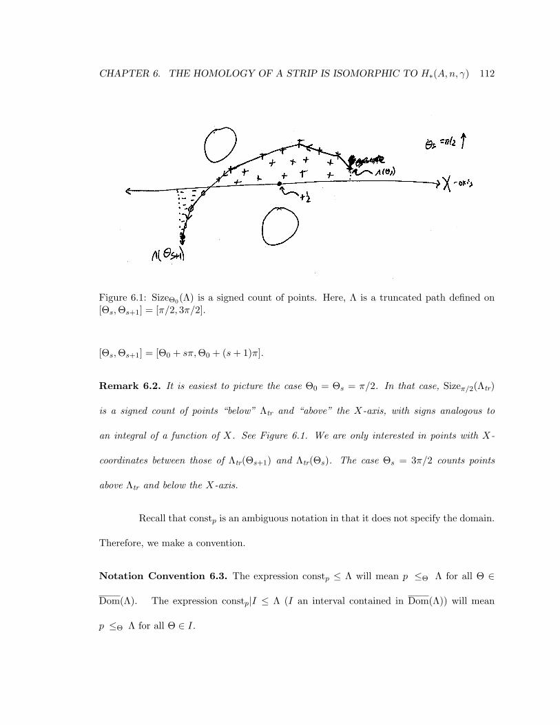
CHAPTER 6. THE HOMOLOGY OF A STRIP IS ISOMORPHIC TO H∗(A,n, γ) 112
Figure 6.1: SizeΘ0(Λ) is a signed count of points. Here, Λ is a truncated path defined on[Θs,Θs+1] = [π/2, 3π/2].
[Θs,Θs+1] = [Θ0 + sπ,Θ0 + (s+ 1)π].
Remark 6.2. It is easiest to picture the case Θ0 = Θs = π/2. In that case, Sizeπ/2(Λtr)
is a signed count of points “below” Λtr and “above” the X-axis, with signs analogous to
an integral of a function of X. See Figure 6.1. We are only interested in points with X-
coordinates between those of Λtr(Θs+1) and Λtr(Θs). The case Θs = 3π/2 counts points
above Λtr and below the X-axis.
Recall that constp is an ambiguous notation in that it does not specify the domain.
Therefore, we make a convention.
Notation Convention 6.3. The expression constp ≤ Λ will mean p ≤Θ Λ for all Θ ∈
Dom(Λ). The expression constp|I ≤ Λ (I an interval contained in Dom(Λ)) will mean
p ≤Θ Λ for all Θ ∈ I.
CHAPTER 6. THE HOMOLOGY OF A STRIP IS ISOMORPHIC TO H∗(A,n, γ) 113
Definition 6.4. If Λtr is a truncated path defined on [Θs,Θs+1], define SizeΘ0(Λtr) as the
sum, for each p ∈ LA,Γ with
p ≤Θs Λtr and p ≤Θs+1 Λtr, (6.4)
of the following:
• +1 if 0 <Θs+π/2 p and constp ≤ Λtr.
• −1 if p <Θs+π/2 0 and constp 6≤ Λtr.
• +12 if p = 0 and constp ≤ Λtr.
• −12 if p = 0 and constp 6≤ Λtr.
• 0 otherwise.
One may imagine that the point 0 is bisected by the X-axis. Recall that 0 ∈ LA,Γ
if and only if Γ = 0, and no other p ∈ LA,Γ lies on the X- or Y -axis, so all other p ∈ LA,Γ
satisfy p <Θs+π/2 0 or 0 <Θs+π/2 p.
We say p contributes positively to SizeΘ0(Λtr) if it appears in the sum with a
positive sign, and similarly for contributes negatively.
The sum appearing in Definition 6.4 is finite, because a sufficiently large rectan-
gular region contains all points that could be included in the sum.
Definition 6.5. If Λ is an (A,n, γ)-periodic path and Θ0 ∈ {π/2, π}, let
SizeΘ0(Λ) =N−1∑s=0
Size(Λ|[Θs,Θs+1]). (6.5)

CHAPTER 6. THE HOMOLOGY OF A STRIP IS ISOMORPHIC TO H∗(A,n, γ) 114
Also let
SizeΘ0(Λ|[Θt,Θu]) =u−1∑s=t
Size(Λ|[Θs,Θs+1]). (6.6)
Lemma 6.6. By periodicity, SizeΘ0(Λ) is also Size(Λ|[Θt,Θt+N ]) for any t.
Lemma 6.7. SizeΘ0 is a relative size function.
In other words, if Λ is an (A,n, γ)-periodic path and c is a proper non-self-rounding
corner of Λ, SizeΘ0(Λ \ c) = SizeΘ0(Λ)− 1.
Proof. Case I: c ⊂ (Θs,Θs+1) for some s. The condition constp ≤ Λ|[Θs,Θs+1] agrees with
the condition constp ≤ (Λ \ c)|[Θs,Θs+1] except for p = Λ(c) (clear from a picture, or see
Proposition 3.69). Passing from Λ to Λ \ c, the sum decreases by one, no matter where p is
relative to 0.
Case II: c 6⊂ (Θs,Θs+1) for any s and N > 1. We may assume c contains some
Θs. Since the length of the interval c is less than π, we may assume c ⊂ [Θs−1,Θs+1]. By
Lemma 6.6, we may assume that both Λ|[Θs−1,Θs] and Λ|[Θs,Θs+1] appear in the sum
defining SizeΘ0(Λ), and they are the only way rounding at c affects Size.
There are no points “in between” Λ|[Θs−1,Θs+1] and (Λ \ c)|[Θs−1,Θs+1] ex-
cept Λ(Θs). Any lattice point such that p ≤Θs (Λ \ c)(Θs) contributes the same to
Size(Λ|[Θs−1,Θs+1]) as to Size((Λ \ c)|[Θs−1,Θs+1]).
Lattice points satisfying p 6≤Θs (Λ\c)(Θs) do not contribute to Size((Λ\c)|[Θt−1,Θt+1]).
We will show that their total contribution to Size(Λ|[Θt−1,Θt+1]) is 1.
The vertices of Λ immediately preceding and immediately following Λ(c) are both
≤Θs (Λ \ c)(c). The triangular region defined by constp ≤ Λ|[Θs−1,Θs+1], p 6 ≤Θs (Λ \ c)(c)

CHAPTER 6. THE HOMOLOGY OF A STRIP IS ISOMORPHIC TO H∗(A,n, γ) 115
contains only Λ(c), which contributes +1 to Size(Λ|[Θs−1,Θs+1]). Any other point≤Θs Λ(c),
6 ≤Θs (Λ \ c)(c) has contribution totaling 0.
Case III: c 6⊂ (Θs,Θs+1) for any s and N = 1.
The proof is similar to Case II, but rounding at c also means rounding at FA,n(c),
so both Λ(Θs) and Λ(Θs+1) are rounded. We have (Λ\c)(Θs+1) ≤Θs (Λ\c)(Θs), so we view
SizeΘ0(Λ) = SizeΘ0(Λ|[Θs,Θs+1]) as the sum of contributions to SizeΘ0(Λ|[Θs,Θs+1]) from
p ≤Θs+1 (Λ\c)(Θs+1) and contributions to SizeΘ0(Λ|[Θs−1,Θs]) from p 6≤Θs (Λ\c)(Θs). This
reformulated count now proceeds the same way as in Case II for the region p 6≤Θs (Λ\c)(Θs).
This sum is affected only by the rounding at Θs, not the rounding at Θs+1, and decreases
by 1 by the reasoning from Case II.
6.2 Bounding SizeΘ0of a flattened path
Lemma 6.8. If Λ is a (B,Θ0)-flattened path and s ∈ Z, then no point contributes negatively
to SizeΘ0(Λ).
Proof. We must show that any p ∈ LA,Γ with
p ≤Θs Λ, (6.7)
p ≤Θs+1 Λ, (6.8)
p ≤Θs+π/2 0 (6.9)
satisfies constp ≤ Λ|[Θs,Θs+1].
The conditions ensure that constp|[Θs,Θs+1] ≤ B. Lemma 5.12 gives a maximality
CHAPTER 6. THE HOMOLOGY OF A STRIP IS ISOMORPHIC TO H∗(A,n, γ) 116
condition for flattened paths, from which constp ≤ Λ|[Θs,Θs+1] follows.
Thus, if Λ is a (B,Θ0)-flattened path, then SizeΘ0(Λ) ≥ 0. We now show that a
certain kind of rectangular region contains points that contribute positively to SizeΘ0(Λ).
Recall that a sufficiently large rectangular region contains as many lattice points as desired
(Lemma 3.75).
Definition 6.9. Given a box or strip B, let Ymin(B) be the minimum of |Y (EdgeB(Θ))|
for horizontal edges (i.e. Θ = kπ) with Θ ∈ [0, 2Nπ]. Similarly, given a box B, let Xmin(B)
be the minimum of |X(EdgeB(Θ))| for vertical edges (Θ = kπ + π/2) with Θ ∈ [0, 2Nπ].
Recall that X(Λ(Θs+N )) = aX(Λ(Θs)); and a, an eigenvalue of A, is not 1.
Lemma 6.10. Given s ∈ {0, 1, . . . , N − 1}, and a (B,Θ0)-flattened Λ with Λ(Θs) 6= 0,
there exists a rectangular region R with sides parallel to the (X,Y )-axes such that every
lattice point in R contributes positively to SizeΘ0(Λ). The region R is the product of two
open intervals, where:
1. If Θ0 = π2 , then R has width |X(Λ(Θs))−X(Λ(Θs+N ))| and height Ymin(B).
2. If Θ0 = π, then R has height |Y (Λ(Θs))− Y (Λ(Θs+N ))| and width Xmin(B).
Here “width” is the measure of the X interval and height is the measure of the Y
interval.
Proof. We may assume Θ0 = π/2. (The other proof is similar.) Since Λ(Θs) 6= 0 and 0 is the
only possible lattice point on the Y -axis, X(Λ(Θs)) 6= 0; so X(Λ(Θs+N )) = aX(Λ(Θs)) 6=
X(Λ(Θs)). We assume
X(Λ(Θs)) > X(Λ(Θs+N )) (6.10)
CHAPTER 6. THE HOMOLOGY OF A STRIP IS ISOMORPHIC TO H∗(A,n, γ) 117
and let
R = (X(Λ(Θs+N ), X(Λ(Θs))× (0, Ymin(B)). (6.11)
The other case is similar, with R = (X(Λ(Θs), X(Λ(Θs+N ))× (−Ymin(B), 0).
Consider p ∈ LA,Γ∩R. We must show p contributes positively to SizeΘ0(Λ). Since
Λ travels from Λ(Θs) to Λ(Θs+N ) and p has itsX-coordinate in between, there is an edge σ of
Λ (with angle Θ ∈ [Θs,Θs+N ]) that crosses the line X = X(p), and we may assume it crosses
going in the −X direction. Therefore σ has angle Θ ∈ [π2 +2πk, 3π2 +2πk] = [Θ2k,Θ2k+1] for
some k ∈ Z. We will show p contributes +1 to SizeΘ0(Λ|[Θ2k,Θ2k+1]). We know p ≤Θ B
for Θ = Θ2k,Θ2k+1 by comparing with σ. We know p ≤Θ2k+π/2 B because Y (p) < Ymin(B).
Thus p ≤Θ B for all Θ ∈ [Θ2k,Θ2k+1]. Then constp ≤ Λ|[Θ2k,Θ2k+1] since Λ is flattened
and the truncated path constp is to the left of B. Thus, since Y (p) > 0, we see that p
contributes +1 to SizeΘ0(Λ).
Corollary 6.11. A (B,Θ0)-flattened path has SizeΘ0(Λ) ≥ |R ∩ LA,Γ|.
There is no issue with counting the origin as +12 because 0 /∈ R.
6.3 Expanding the box
The following lemma will show Hi(B) ∼= Hi(B′), for sufficiently large boxes B, B′
with B′ wider than B in the horizontal direction, using flattening with Θ0 = π/2.
Lemma 6.12. Suppose i ∈ Z and Yi > 0. There exists Xi > 0 such that for any (A,n, γ)-
boxes B,B′ with Xmin(B) ≥ Xi and Ymin(B) ≥ Yi, and B ≤ B′ and
Y (EdgeB(Θ)) = Y (EdgeB′(Θ)) (6.12)

CHAPTER 6. THE HOMOLOGY OF A STRIP IS ISOMORPHIC TO H∗(A,n, γ) 118
for all horizontal edges, we have: Cflat∗ (B, π/2) is a subcomplex of Cflat
∗ (B′, π/2), and the
inclusion induces an isomorphism
Hflati (B, π/2) ≈→ Hflat
i (B′, π/2). (6.13)
Proof. To show Cflat∗ (B, π/2) ⊆ Cflat
∗ (B′, π/2), note that the flattened path Λ satisfying
Λ(Θs) = psbs depends only on the horizontal edges of B or B′, not the vertical ones; and the
in-range-ness of {ps} depends on B only by ps ∈ �B,Θs , and we have �B,Θs ⊆ �B′,Θs .
The inclusion of flattened chain complexes induces a map on homology which will
be an isomorphism in degree i once we show that “new” flattened generators ((B′, π/2)-
flattened generators that are not (B, π/2)-flattened generators) have index ≥ i+ 2.
A (B′, π/2)-flattened path Λ that is not a (B, π/2)-flattened path has Λ(Θs) =
ps /∈ �B,Θs for some s. We may choose s ∈ {0, . . . , N − 1} with Λ(Θs) 6 ≤Θs EdgeB(Θs).
The path satisfies
Sizeπ/2(Λ) ≥ |LA,Γ ∩R| (6.14)
where R is the rectangular region from Lemma 6.10. That region has height Ymin(B′) ≥ Yi.
The width is |X(Λ(Θs)) − X(Λ(Θs+N ))|, but X(Λ(Θs+N )) = aX(Λ(Θs)) so the width is
|1 − a||X(Λ(Θs))|. But |X(Λ(Θs))| ≥ |X(EdgeB(Θs))| ≥ Xmin(B), and thus the width is
≥ |1− a|Xmin(B) ≥ |1− a|Xi.
Lemma 3.75 asserts that for fixed height, a rectangle may be made to contain as
many points as desired by changing the width. In our case, for fixed Yi, we may obtain
Sizeπ/2(Λ) as large as desired by choosing |1−a|Xi large enough (note that 1−a 6= 0). The
index of a flattened generator is
I( [Λ; {ηs}] ) = 2 Sizeπ/2(Λ)−#h{ηs}+ iπ/2 (6.15)

CHAPTER 6. THE HOMOLOGY OF A STRIP IS ISOMORPHIC TO H∗(A,n, γ) 119
where iπ/2 (which depends on (A,n, γ)) is independent of B and B′. Since we may make
Sizeπ/2(Λ) as large as desired, we may make I( [Λ; {ηs}] ) larger than i + 2. (Note that
#h{ηs} ≤ N . Since (A,n, γ) are fixed throughout, so is N .)
Lemma 6.13. Suppose i ∈ Z and Yi > 0. There exists X ′i > 0 such that for any (A,n, γ)-
boxes B and B′ with Xmin(B) ≥ X ′i and Ymin(B) ≥ Yi and B ≤ B′, and
X(EdgeB(Θ)) = X(EdgeB′(Θ)) (6.16)
for all vertical edges (i.e. for Θ = π/2 + sπ for all s ∈ Z), we have: Cflat∗ (B, π) is a
subcomplex of Cflat∗ (B′, π), and the inclusion induces an isomorphism
Hflati (B, π) ≈→ Hflat
i (B′, π). (6.17)
The above claim is similar to Lemma 6.12, with the roles of X and Y mostly
reversed. We still fix Yi, because our goal involves strips parallel to the X-axis.
Proof. The proof is similar to that of Lemma 6.12. For each Yi, we must choose X ′i so
as to get enough points in a rectangle with width ≥ X ′i and height |1 − a−1||Y (Λ(Θs))| ≥
|1− a−1|Yi (and 1− a−1 6= 0). This can be done, by Lemma 3.75.
Lemma 6.14. Suppose i ∈ Z and Yi > 0. If B and B′′ are (A,n, γ)-boxes with B ≤ B′′,
Xmin(B) ≥ max(Xi, X′i) (with Xi, X ′i as in Lemmas 6.12 and 6.13), and Ymin(B) ≥ Yi,
then
C∗(B) ↪→ C∗(B′′) (6.18)
induces an isomorphism
Hi(B) ≈→ Hi(B′′). (6.19)
CHAPTER 6. THE HOMOLOGY OF A STRIP IS ISOMORPHIC TO H∗(A,n, γ) 120
Proof. We may pass from B to B′′ by first expanding B horizontally to B′, then vertically
to B′′, applying Lemmas 6.12 and 6.13. We have Hi(B) ∼= Hflati (B, π/2) ∼= Hflat
i (B′, π/2) ∼=
Hi(B′) and similarly Hi(B′) ∼= Hi(B′′) (using π in place of π/2). Thus Hi(B) and Hi(B′′)
are isomorphic. We must show that the isomorphism Hi(B)∼=→ Hi(B′) is induced by
C∗(B)→ C∗(B′) (and similarly for B′ to B′′). But the inclusions
Cflati (B, π/2) //
��
Cflati (B′, π/2)
��Ci(B) // Ci(B′)
(6.20)
commute and induce commuting maps on Hi. We already knew that three of those maps
are isomorphisms, so Hi(B)→ Hi(B′) is also an isomorphism.
6.4 Taking the direct limit
We restate Theorem 6.1.
Theorem 6.15. Given an (A,n, γ)-strip B∞, the inclusion C∗(B∞) ↪→ C∗(A,n, γ) induces
an isomorphism H∗(B∞) ≈→ H∗(A,n, γ).
Proof. Fix i ∈ Z. Let Yi = Ymin(B∞). LetB be formed by shortening the horizontal edges of
B∞ (so Y (EdgeB(Θ)) = Y (EdgeB∞(Θ)) for horizontal edges) and putting in vertical edges
sufficiently far from the origin, so Xmin(B) is bigger than both Xi, X′i from Lemma 6.12
and Lemma 6.13. (These finitely many constrains on vertical edges may be satisfied while
respecting periodicity.)
Then for any B′ with B ≤ B′ we have that C∗(B) ↪→ C∗(B′) induces an isomor-
CHAPTER 6. THE HOMOLOGY OF A STRIP IS ISOMORPHIC TO H∗(A,n, γ) 121
phism on Hi. Forming a sequence {B′k} that exhausts the plane,
Hi(B) ∼= lim−→Hi(B′k) ∼= Hi(A,n, γ), (6.21)
with Hi(B) ≈→ Hi(A,n, γ) induced by the inclusion of chain complexes. Form a sequence
{B′′k} with horizontal edges matching B∞ (and B), exhausting B∞, we have
Hi(B) ∼= lim−→Hi(B′′k) ∼= Hi(B∞), (6.22)
with Hi(B) ≈→ Hi(B∞) induced by the inclusion of chain complexes. Furthermore the
commutative diagram of inclusions
C∗(B) //
&&MMMMMMMMMMC∗(B∞)
��C∗(A,n, γ)
(6.23)
yields a commutative diagram of isomorphisms of Hi, so C∗(B∞) ↪→ C∗(A,n, γ) induces an
isomorphism on Hi. This holds for all i.

122
Chapter 7
The n = 1 case
This chapter computes H∗(A, 1, γ). We already have everything needed for some
matrices A:
Theorem 7.1. Suppose A is negative hyperbolic or −1, n = 1, and Γ ∈ Z2/ Im(1−A) with
γ ∈ Γ. Then
Hi(A,n, γ) ∼=
Z if i ≥ i0
0 if i < i0,
(7.1)
where i0 ∈ Z is as in Proposition 5.35.
Proof. Combine Theorem 5.36 and Theorem 6.1.
In the current chapter, we calculate Hi(A, 1, γ) for positive hyperbolic A.
For the remainder of this chapter, fix A positive hyperbolic, let n = 1, and fix
Γ ∈ Z2/ Im(1−A) with γ ∈ Γ. As usual, γ = 0 if and only if Γ = 0. Note that N = 2.
CHAPTER 7. THE n = 1 CASE 123
Theorem 7.2. 1. If γ = 0, then
Hi(A, 1, 0) ∼=
Z if i > 0
Z2 if i = 0
0 if i < 0.
(7.2)
2. If Γ 6= 0 with γ ∈ Γ, then
Hi(A, 1, γ) ∼=
Z if i ≥ i0
0 if i < i0
(7.3)
where i0 ∈ Z is as in Proposition 5.35.
This theorem will follow from a calculation of the homology of a strip (using
Theorem 6.1). Fix an (A, 1, γ)-strip B∞.
Proposition 7.3. 1. If γ = 0, then
Hflati (B∞, π/2) ∼=
Z if i > 0
Z2 if i = 0
0 if i < 0.
(7.4)
2. If Γ 6= 0 with γ ∈ Γ, then
Hflati (B∞, π/2) ∼=
Z if i ≥ i0
0 if i < i0
(7.5)
where i0 ∈ Z is as in Proposition 5.35.
Proving Proposition 7.3 will take the rest of the chapter.

CHAPTER 7. THE n = 1 CASE 124
7.1 Description of the chain complex
7.1.1 Flattened generators for N = 2
In this subsection, we will give a description of the structure of the chain complex
Cflat∗ (B∞). The main result of this section is Proposition 7.22 below.
We recall (and summarize) the results of the previous chapters, specializing to
N = 2.
Recall that Cflat∗ (B∞) is generated (over Z) by flattened generators [b0, b1; η0, η1]
where b0, b1 ∈ Z or Z + 12 index flattening points and η0, η1 ∈ {‘E’, ‘H’} describe labels.
We may say that the chain complex is freely generated by those flattened generators which
satisfy certain inequalities, or that it is a quotient, setting some [b0, b1; η0, η1] = 0. Viewing
the chain complex as a quotient will allow δ to be more concisely stated.
Here, the pair (b0, b1) (or equivalently the 2-periodic sequence {. . . , b0, b1, b0, b1, . . .})
describes the shape of the flattened path and (η0, η1) (or the 2-periodic sequence) describes
its labeling. Formally:
1. The abelian group Cflat∗ (B∞) is generated by all formal expressions [b0, b1; η0, η1]
where b0, b1 ∈ Z if Γ = 0, or Z + 12 if Γ 6= 0, and η0, η1 ∈ {‘E’, ‘H’}; modulo
[b0, b1; η0, η1] = 0 (7.6)
unless the following conditions hold:
X(p1b1) ≤ X(p0
b0), X(p1b1) ≤ X(p2
b0) (7.7)
p0b0 = p1
b1 implies η0 = ‘E’ (7.8)
p1b1 = p2
b0 implies η1 = ‘E’. (7.9)
CHAPTER 7. THE n = 1 CASE 125
Here, psbs is a certain lattice point indexed by bs, as in Chapter 5. Of course, X(p) is
the X-coordinate (using eigencoordinates) of p. Also, periodicity allows us to write
p2b2
as p2b0
. If the conditions (7.7)–(7.9) hold, we say ((b0, b1), (η0, η1)) is in range and
[b0, b1; η0, η1] is a flattened generator. (Otherwise, it is 0, which is not a flattened
generator.)
2. The index of [b0, b1; η0, η1] is 2(b0 + b1) + i0 −#H, where i0 ∈ Z is a constant, and
#H denotes the number of ‘H’ labels. If Γ = 0, then i0 = 0.
3. The differential, δ, on Cflat∗ (B∞) is as follows:
[b0, b1;EE] 7→ 0
[b0, b1;EH] 7→ [b0 − 1, b1;EE] − [b0, b1 − 1;EE]
[b0, b1;HE] 7→ − [b0 − 1, b1;EE] + [b0, b1 − 1;EE]
[b0, b1;HH] 7→ − [b0 − 1, b1;EH] − [b0 − 1, b1;HE]
+ [b0, b1 − 1;EH] + [b0, b1 − 1;HE] ,
(7.10)
where we have dropped unnecessary punctuation from [b0, b1; ‘E’, ‘E’] , and we are
taking advantage of the quotient definition of Cflat∗ (B∞) to describe δ concisely. The
expressions on the right-hand side are sometimes 0. Furthermore, the signs stated take
advantage of our convention on the ordering of ‘H’ labels for flattened generators (η0
before η1).
We frequently work with the pairs (b0, b1) which encode just the flattened path
and not its labeling. If (7.7) holds, we say (b0, b1) is in range, which is equivalent to
((b0, b1), (‘E’, ‘E’)) being in range, i.e. [b0, b1;EE] 6= 0.
CHAPTER 7. THE n = 1 CASE 126
Notation Convention 7.4. When there is a pair named (b0, b1), we let
X0 = X(p0b0) (7.11)
X1 = X(p1b1) (7.12)
X2 = X(p2b0). (7.13)
By periodicity, X2 is also X(p2b2
) = aX0, where a is the eigenvalue of A with a > 1
(here A is positive hyperbolic). We can rewrite (7.7)–(7.9) as
X1 ≤ X0, X1 ≤ X2 (7.14)
X0 = X1 implies η0 = ‘E’ (7.15)
X1 = X2 implies η1 = ‘E’. (7.16)
Recall that no two lattice points have the same X-coordinate, allowing us to replace “p = p”
with “X = X”.
7.1.2 “EH-maximal”, etc.
Our first goal is to figure out exactly which data((b0, b1), (η0, η1)
)are in range, i.e.
which define flattened generators [b0, b1; η0, η1] . Our convention is that out-of-range data
result in [b0, b1; η0, η1] = 0, which we do not call a “flattened generator”.
For fixed (b0, b1), the labeling with the most ‘H’ ’s determines what labelings are
allowed.
Lemma-Definition 7.5. For any (b0, b1) (with bs ∈ Z or Z + 12 depending on Γ), one of
the following is the case regarding the four expressions [b0, b1; η0, η1] for η0, η1 ∈ {‘E’, ‘H’}:
0. All [b0, b1; η0, η1] are 0. (Recall that we say (b0, b1) is out of range in this case.)
CHAPTER 7. THE n = 1 CASE 127
1. Only [b0, b1;EE] is nonzero. We say that (b0, b1) is EE-maximal.
2. Both [b0, b1;EE] and [b0, b1;EH] are nonzero, and the other two are 0. We say that
(b0, b1) is EH-maximal.
3. Both [b0, b1;EE] and [b0, b1;HE] are nonzero, and the other two are 0. We say that
(b0, b1) is HE-maximal.
4. All four [b0, b1; η0, η1] ’s are nonzero; we say that (b0, b1) is HH-maximal.
Proof. The conditions on ‘E’ and ‘H’ labels either allow both labels, or only allow ‘E’, in
any given spot.
Lemma 7.6. The pair (b0, b1) is EE-maximal if and only if (b0, b1) = (0, 0), in which case
γ = 0.
Proof. We need to check that having only [b0, b1;EE] be nonzero is equivalent to (b0, b1) =
(0, 0) and γ = 0. It is clear from (7.8) and (7.9) that having only [b0, b1;EE] be nonzero is
equivalent to p0b0
= p1b1
= p2b0
(which takes care of (7.7)). But p0b0
=(a 00 a−1
)p0b0
means p0b0
is at 0, and so is p1b1
. These points can only be at 0 when 0 ∈ LA,Γ, which is equivalent to
Γ = 0 and to γ = 0. In this case, b0 = 0 and b1 = 0.
Recall that we refer to (b0, b1) as being in range if((b0, b1), (E,E)
)is in range.
It is clear from the conditions defining “in range” that if((b0, b1), (η0, η1)
)is in range –
i.e., [b0, b1; η0, η1] is nonzero – then (b0, b1) is in range. Thus, examining in-range (b0, b1)’s
is equivalent to examining the flattened generators of the form [b0, b1;EE] . Flattened
generators with other labels (other {ηs}) will occur only for in-range pairs (b0, b1). The
index of [b0, b1;EE] is 2(b0 + b1) if Γ = 0, and 2(b0 + b1) + i0 for some constant i0 if Γ 6= 0.
CHAPTER 7. THE n = 1 CASE 128
We call the set of in-range pairs with b0 + b1 fixed a level because we imagine
drawing a picture with b0 + b1 increasing as one goes up. (The b0 and b1 axes are diagonal.)
The diagram will turn out to be an infinite ∨, with ragged edges. Note that b0 +b1 ∈ Z even
if bs ∈ Z + 12 . For each level, there is a “segment” of in-range pairs (see Definition 7.16),
and the segments get strictly wider as one goes up, i.e., as b0 + b1 increases.
Lemma 7.7. When b0, b1 ≥ 0, with (b0, b1) 6= (0, 0), then (b0, b1) is HH-maximal. When
b0, b1 ≤ 0, with (b0, b1) 6= (0, 0), then (b0, b1) is out of range.
In other words, [b0, b1; η0, η1] is always nonzero in the first case and [b0, b1; η0, η1]
is always zero in the second case.
Proof. In the first case, b0 or b1 is positive; say b0 > 0, b1 ≥ 0. Then X0 > 0, X1 ≤ 0,
X2 > 0. This gives X1 < X0, X2 (which we also get if b0 ≥ 0, b1 > 0). Then (7.14)–(7.16)
are satisfied and [b0, b1; η0, η1] 6= 0. If b0 < 0, b1 ≤ 0, then X0 < 0, X1 ≥ 0, contradicting
(7.14), so [b0, b1; η0, η1] = 0, and similarly if b0 ≤ 0, b1 < 0.
If (b0, b1) is in range, then the entire ∨-shaped region “above” (b0, b1) is HH-
maximal.
Lemma 7.8. If (b0, b1) is in range, and if b′0 ≥ b0, b′1 ≥ b1 with (b′0, b′1) 6= (b0, b1), then
(b′0, b′1) is HH-maximal.
In particular, (b0 + 1, b1) and (b0, b1 + 1) are in range.
Proof. Increasing b0 or b1 moves X0 and X2, or X1, in the “good” direction, making it
easier to satisfy (7.7), so (b′0, b′1) is in range. Further, we now have strict inequalities,
X1 < X0, X1 < X2, (7.17)

CHAPTER 7. THE n = 1 CASE 129
which make (7.15) and (7.16) trivial, allowing all ‘H’ labels.
7.1.3 Neighbors of an in-range pair
We now examine the other two “quadrants”, starting with the case b0 > 0, b1 < 0.
(In these quadrants, the points that b0 and b1 index are on the same side of the Y axis and
have a chance of violating the definition of in range).
Remark 7.9. Condition (7.14) is sensitive to min{X0, X2}. Since X2 = aX0 with a > 1,
that means it is X0 (which is positive) that matters when b0 > 0 and X2 when b0 < 0.
We begin by considering one pair (b0, b1) at a time.
Lemma 7.10. We consider two cases.
1. When b0 > 0, b1 < 0 we have:
• If X1 < X0 then (b0, b1) is HH-maximal.
• If X1 = X0 then (b0, b1) is EH-maximal.
• If X1 > X0 then (b0, b1) is out of range.
2. When b0 < 0, b1 > 0 we have:
• If X1 < X2 then (b0, b1) is HH-maximal.
• If X1 = X2 then (b0, b1) is HE-maximal.
• If X1 > X2 then (b0, b1) is out of range.
Proof. We will only show part 1; the proof of part 2 is similar. To do that, we need only
verify that X1 < X2 in the first two cases, the ones with X1 ≤ X0. (Everything else is a
CHAPTER 7. THE n = 1 CASE 130
straightforward application of (7.14)–(7.16).) But
X1 ≤ X0 < aX0 = X2. (7.18)
Now we relate (b0, b1) to its neighbors. The crucial fact is that the points indexed
as p1b1
are a subset of those indexed as p0b0
. In turn, the points indexed as p2b0
are a subset
of those indexed as p1b1
.
Lemma 7.11.
{p2b | b ∈ Z or Z + 1
2} ⊂ {p1b | b ∈ Z or Z + 1
2}
⊂ {p0b | b ∈ Z or Z + 1
2}.(7.19)
Furthermore, there are infinitely many points p0b with b > 0 that are not of the form p1
b′,
and infinitely many with b < 0. A similar statement is true relating p2 and p1.
As elsewhere in this subsection, we are working with A positive hyperbolic. A
similar result is true for A negative hyperbolic, but not for A = −1.
Proof. The idea is that each successive set lies in a narrower region �B,Θs . Each set men-
tioned is the set of lattice points between two lines bounding the strip B∞, and the lines
get closer together as s (in ps) increases. More formally, if points p0b have Y -coordinate in
an interval [−Y0, Y1], then points p1b lie in [− 1
aY0, Y1], and points p2b in [− 1
aY0,1aY1].
The infinitely many points p0b (b > 0) not of the form p1
... are the infinitely many
lattice points in the region defined by X > 0, Y ∈ [−Y0,− 1aY0) (i.e. in the region for p0
minus the region for p1). Here, a > 1. This region has infinitely many points by Lemma 3.75
on the number of points in an open rectangle, such as (X,Y ) ∈ (0,∆X) × (−Y0,− 1aY0);

CHAPTER 7. THE n = 1 CASE 131
the lemma shows that the number of lattice points may be made as large as desired by a
suitable choice of ∆X. The analogous results for b0 < 0 and for points p2... not of the form
p1... follow similarly.
From Lemma 7.11, we will deduce several things. We must first treat the case
bs = 1/2 with b0 + b1 < 0 by itself.
Lemma 7.12. Assume Γ 6= 0 and b0 + b1 < 0. If b0 = 1/2, or b1 = 1/2, then (b0, b1) is out
of range.
Proof. As usual, we prove only one half of the statement: Assume b0 = 1/2. Then b1 <
−1/2, so since b1 ∈ Z + 12 , we have b1 ≤ −3/2. Then p0
b0is the lattice point (with Y in the
appropriate interval) with the smallest positive X coordinate. But p1− 1
2
is the lattice point
with the smallest positive X in a smaller Y -interval, so it is at least as big: X(p0b0
) ≤ X(p1− 1
2
)
so X(p0b0
) < X(p1− 3
2
) ≤ X(p1b1
). Thus (7.7) is violated and (b0, b1) is out of range.
Now we treat the remaining part of the quadrant b0 > 0, b1 < 0 (as well as the
quadrant b1 > 0, b0 < 0). Assuming b0 > 0 and ignoring b0 = 1/2, we may assume b0 ≥ 1.
Furthermore, it turns out not to be necessary to assume b1 < 0.
Lemma 7.13. If (b0, b1) is in range with b0 ≥ 1, then (b0 − 1, b1 + 1) is also in range. If
(b0, b1) is in range with b1 ≥ 1, then (b0 + 1, b1 − 1) is also in range.
Proof. We prove only the first statement. The reason it is true is that while we have moved
p1b1
“one step” left, we have moved p0b0
left by a possibly smaller amount, since p0 indexes a
larger set of points. If p0b0
was on the correct side of p1b1
before the move, the resulting points
after the move are certainly on the correct sides. Formally, count the points p0c , c ∈ Z or

CHAPTER 7. THE n = 1 CASE 132
Z+ 12 , “between” p1
b1+1 and p0b0−1 in the sense of having X-coordinate greater than X(p1
b1+1)
and less than X(p0b0−1). That number of points will be at least as great as the number
between p1b1
and p0b0
in the same sense of “between”. We impose b0 ≥ 1 to get the condition
b0− 1 ≥ 0 which ensures X(p2b0−1) ≥ 0 and therefore X(p2
b0−1) = aX(p0b0−1) ≥ X(p0
b0−1), so
that p2 cannot cause a problem.
It follows from the above lemmas that the set of in-range (b0, b1) with some fixed
b0 + b1 is “connected” in the obvious sense. (Lemma 7.17 will show that that connected set
is finite.)
Definition 7.14. For l ∈ Z, call the set of in-range (b0, b1) with b0 + b1 = l connected if
there is an interval I (possibly empty or unbounded) such that (b0, b1) with b0 +b1 = l (and
with b0, b1 ∈ Z or Z + 12 as usual) is in range if and only if b0 ∈ I.
Lemma 7.15. The set of in-range (b0, b1) with b0 + b1 = l is always connected. It is
nonempty if l > 0 or if l = 0 and Γ = 0. It is empty if l < 0.
Proof. For l = b0 + b1 > 0 (any Γ), or for l = 0 (Γ = 0), we apply Lemma 7.13 repeatedly,
moving from (b0, b1) “inwards” to (b0 ∓ 1, b1 ± 1), towards the pairs known to be in range,
those with b0, b1 ≥ 0. (These are known to be in range by Lemma 7.7 when (b0, b1) 6= (0, 0)
and Lemma 7.6 when (b0, b1) = (0, 0).) More precisely, suppose (b0, b1) is in range, with
b0+b1 = l; then b0 and b1 are both nonnegative, which is the known case, or one of them (say
b1) is negative. Then b1 < 0 means b0 = l − b1 > l ≥ 0, so b0 > 0. In fact b0 ≥ 1, because
if Γ = 0 then b0 ∈ Z, and if Γ 6= 0 we are assuming l > 0. Thus we can apply Lemma 7.13
and move “left”, showing each pair is in range until we have reached the b0, b1 ≥ 0 region.
CHAPTER 7. THE n = 1 CASE 133
Similar considerations for Γ 6= 0 show that level l = 0 is connected (possibly
empty). In this case, we consider the regions b0 > 0 and b1 > 0 (here, b1 = −b0) separately.
In each, we may apply Lemma 7.13 repeatedly, moving toward the center until we reach
the last point, (b0, b1) = ±(
12 ,−
12
); we cannot apply Lemma 7.13 to that point. Thus the
in-range pairs with b0 + b1 = 0 and b0 > 0 form either the empty set or a connected set
containing(
12 ,−
12
); and similarly for those with b1 > 0. There are now four cases, depending
on which of the points ±(
12 ,−
12
)are in range. But these two points are “adjacent”, so we
have that level l = 0 is connected (possibly empty).
For l < 0, we already have that some pairs are out of range. Specifically, those
with b0, b1 ≤ 0, for all Γ. For Γ 6= 0, we may expand this region (using Lemma 7.12) to:
If b0, b1 ≤ 12 with b0 + b1 < 0, then (b0, b1) is out of range. For any (b0, b1) outside of this
region, Lemma 7.13 allows us to move towards the region known to be out of range, so
(b0, b1) cannot be in range. Thus, there are no in-range pairs with b0 + b1 < 0.
We define a segment to be a finite, nonempty, connected set of pairs.
Definition 7.16. A segment in level l is a set of ordered pairs (b0, b1) ∈ Z2 or (Z + 12)2 of
the following form: Fix endpoints (c0, c1) and (d0, d1) with c0 + c1 = d0 + d1 = l. We may
assume c0 ≤ d0 (and therefore c1 ≥ d1). The segment with these endpoints is
{(b0, b1) | b0 + b1 = l and c0 ≤ b0 ≤ d0}. (7.20)
Of course, we may equivalently require c1 ≥ b1 ≥ d1.
Lemma 7.17. For any l ∈ Z, there are only finitely many in-range pairs (b0, b1) with
b0 + b1 = l.
CHAPTER 7. THE n = 1 CASE 134
This statement is close to some results of Chapter 6, but we will prove it directly.
Proof. We will show that (k+ l,−k) is out of range for a sufficiently large positive choice of
k ∈ Z or Z+ 12 . (A similar argument which we will not state applies to (−k, l+k), completing
the proof.) Specifically, we will show that X(p1−k) > X(p0
k+l). There are infinitely many
points of the form p0b (b > 0, i.e., X > 0) not of the form p1
b′ , so consider the (l + 1)’th
such point and call it p0k′ (so k′ > 0). There being infinitely many points p1
−k (k > 0), and
these points being a discrete set, there is some p1−k “after” p0
k′ , i.e., X(p0k′) < X(p1
−k). Our
numbering conventions mean that p1−k is the k’th point (or (k + 1
2)’th point) in the X > 0
part of the p1 region defined by the strip B∞. But it must be at least the (k+ l+1)’th point
(or (k+ l+ 32)’th point) in the p0 region, and in particular, p0
k+l+1 must come “sooner” (not
strictly):
X(p0k+l+1) ≤ X(p1
−k). (7.21)
Then, taking another point, one “sooner” than before,
X(p0k+l) < X(p1
−k), (7.22)
as desired.
We now have sufficient information about which (b0, b1) are in range.
Proposition 7.18. Let A be positive hyperbolic, n = 1, and Γ ∈ Z2/ Im(A−1) with γ ∈ Γ.
For any l ∈ Z, the set of in-range pairs (b0, b1) with b0 + b1 = l is a segment if l > 0 and
empty if l < 0. If Γ = 0 and l = 0, the set is a segment. If Γ 6= 0 and l = 0, the set is either
empty or a segment. The segment at index l+ 1 is wider than the one at index l (whenever
both are nonempty); formally, if (b0, b1) is in range, then so are (b0 + 1, b1) and (b0, b1 + 1).

CHAPTER 7. THE n = 1 CASE 135
Proof. Most of the statement of this proposition just applies the finiteness result of Lemma
7.17 to the statement of Corollary 7.15. The last sentence follows from Lemma 7.8, which
implies that each level is wider than the one below it.
We will not describe the set of in-range pairs any more precisely–we will not specify
the shape of the ragged edges of the ∨. To do so would require considering the details
of where lattice points fall in the strip in question, which depends on A. However, just
knowing Proposition 7.18 and some information about labels will be sufficient to determine
the homology. That is the reason that the homology for positive hyperbolic A is essentially
independent of A.
7.1.4 Return to EH-maximal, etc.
To finish describing the generators of Cflat∗ (B∞), we must determine which la-
bels are possible. That is, for each in-range (b0, b1), we find out which (η0, η1) make
[b0, b1; η0, η1] 6= 0. Lemma 7.6 already shows that only (0, 0) is EE-maximal. It will
turn out that the distinction between EH-maximal and HE-maximal is not important.
We must find which in-range pairs are HH-maximal. Lemma 7.8 shows that within any
segment of in-range pairs, the set of HH-maximal pairs is at least as big as needed to
“cover” the segment below. We will soon show that it is exactly big enough. First, we have
a preparatory lemma.
Lemma 7.19. Suppose (b0, b1) is HH-maximal. If b0 > 0, b1 < 0, then (b0 − 1, b1) is in
range. If b0 < 0, b1 > 0, then (b0, b1 − 1) is in range.
Proof. We prove the first case, assuming X1 < X0, X1 < X2 by HH-maximality, and that

CHAPTER 7. THE n = 1 CASE 136
each Xs is positive by the inequalities on the bs’s. Intuitively, the worst that p0b0−1 could
be (the smallest X) is p1b1
. Formally, since the p1’s are a subset of the p0’s,
p1b1 = p0
c for some c, (7.23)
and since 0 < X1 < X0, i.e. 0 < X(p0c) < X(p0
b0), we must have 0 < c < b0. (Incidentally,
this fact already means b0 ≥ 3/2.) We need b0− 1 and its lattice point p0b0−1; but c ≤ b0− 1
so X(p0c) ≤ X(p0
b0−1), i.e.
X(p1b1) ≤ X(p0
b0−1). (7.24)
We still have b0 − 1 > 0, so p2 cannot cause a problem:
X(p1b1) ≤ X(p2
b0−1), (7.25)
by reasoning as in Lemma 7.10. Thus, (b0 − 1, b1) is in range.
Corollary 7.20. An in-range pair (b0, b1) other than (12 ,
12) is HH-maximal if and only if
at least one of the pairs “below” it, (b0 − 1, b1) and (b0, b1 − 1), is in range.
Proof. “If” follows from Lemma 7.8. “Only if” follows by cases:
1. If b0 > 0, b1 < 0, or vice versa, apply Lemma 7.19.
2. If b0, b1 ≤ 0, then Lemma 7.7 tells us that (b0, b1) is out of range (so the claim is
trivially true) unless (b0, b1) = (0, 0) (in which case the claim follows because (−1, 0)
and (0,−1) are out of range).
3. If b0, b1 ≥ 0, (b0, b1) 6= (0, 0), then Lemma 7.7 tells us that (b0, b1) is HH-maximal.
But if we also have (b0, b1) 6= (12 ,
12), then one of (b0 − 1, b1) and (b0, b1 − 1) is also in
this same region or is (0, 0), and in either case, is in range.

CHAPTER 7. THE n = 1 CASE 137
We now have the tools to establish our result. Informally, each segment, except
at level 0, contains zero or more HE-maximal cells, then one or more HH-maximal cells
“covering” the segment below, and then zero or more EH-maximal cells. The only EE-
maximal cell appears in level l = 0, at the pair (0, 0), when Γ = 0. More precisely, level 0
contains zero or more HE-maximal cells, then one EE-maximal cell if Γ = 0, then zero or
more EH-maximal cells.
Definition 7.21. Given a segment S of ordered pairs with endpoints (c0, c1) and (d0, d1)
(we assume c0 ≤ d0), the segment S′ covering S is the segment with endpoints (c0, c1 + 1)
and (d0 + 1, d1).
Note that S′ is in level l + 1 if S is in level l, and that S′ has one more element
than S. (It is “one wider” than S.)
Proposition 7.22. Let A be positive hyperbolic, n = 1, and Γ ∈ Z2/ Im(A−1) with γ ∈ Γ.
For each l ∈ Z, the flattened generators with l = b0 + b1 are as follows.
1. If l < 0, there are no generators.
2. If l = 0, there are no HH-maximal pairs. There is an EE-maximal pair (at (0, 0)) if
and only if Γ = 0. The part of l = 0 with b1 > 0 has zero or more HE-maximal pairs.
The part of l = 0 with b0 > 0 has zero or more EH-maximal pairs.
3. If l > 0, the set of pairs (b0, b1) which are HH-maximal are exactly the segment S′
covering the segment S of in-range pairs in level l − 1, if S is nonempty. Otherwise,
S = ∅ and there is a single HH-maximal pair, (12 ,
12) in level 1; let S′ = {(1
2 ,12)}.

CHAPTER 7. THE n = 1 CASE 138
“Left” of S′ (i.e., larger b1), we have zero or more HE-maximal pairs. “Right” of S′
(i.e., larger b0), we have zero or more EH-maximal pairs.
Proof. 1. Already shown (see Lemma 7.15).
2. In this case, there are no HH-maximal pairs by Corollary 7.20. Most of the rest of
the claim follows from Lemma-Definition 7.5. To distinguish HE- from EH-maximal
pairs, note that b0 and b1 have opposite signs in level 0, and apply the two halves of
Lemma 7.10.
3. The statement that S′ covers nonempty S follows from Corollary 7.20 if l > 1, or if
l = 1 and Γ = 0. It also follows if l = 1, Γ 6= 0, and level 0 is nonempty (then the
claim of Corollary 7.20 is true even of (12 ,
12), which is HH-maximal by Lemma 7.7).
If level 0 is empty, Corollary 7.20 prevents any HH-maximal pairs other than (12 ,
12),
proving the claim about S′ = ∅. The remaining pairs must be HE- or EH-maximal
and cannot lie in Lemma 7.7’s region b0, b1 ≥ 0, so they must fall under one of the
two halves of Lemma 7.10, which makes the ones with b1 > 0 HE-maximal, and vice
versa.
7.2 The homology
Now that we have determined what is in the chain complex Cflat∗ (B∞), we will
compute its homology.
We will describe the action of the boundary map δ, following a change of basis.

CHAPTER 7. THE n = 1 CASE 139
Definition 7.23. Let
[b0, b1;H] = [b0, b1;EH] + [b0, b1;HE] . (7.26)
This notation is useful even when one (or both!) of the expressions on the right-
hand side are zero.
If (b0, b1) is EH-maximal or HE-maximal, it has two generators, [b0, b1;EE] and
[b0, b1;H] , in the new basis.
If (b0, b1) is HH-maximal, we still need [b0, b1;EH] , and we introduce notation:
Definition 7.24. Let
[b0, b1;EH ′] = [b0, b1;EH] (7.27)
if (b0, b1) is HH-maximal, and
[b0, b1;EH ′] = 0 (7.28)
otherwise.
Lemma 7.25. The differential δ on Cflat∗ (B∞) acts as follows:
[b0, b1;EE] 7→ 0 (7.29)
[b0, b1;H] 7→ 0 (7.30)
[b0, b1;EH ′] 7→ − [b0 − 1, b1;EE] + [b0, b1 − 1;EE] (7.31)
[b0, b1;HH] 7→ − [b0 − 1, b1;H] + [b0, b1 − 1;H] . (7.32)
Recall that we use, as always, the convention that [b0, b1; η0, η1] = 0 when ((b0, b1), (η0, η1))
is out of range.
CHAPTER 7. THE n = 1 CASE 140
Proof. The result follows directly from item 3 on page 125 and our new definitions.
Now we have found the structure of the chain complex. We may now compute the
homology, proving Proposition 7.3 and thus Theorem 7.2. We restate Proposition 7.3:
Proposition 7.26. 1. If γ = 0, then
Hflati (B∞, π/2) ∼=
Z if i > 0
Z2 if i = 0
0 if i < 0.
(7.33)
2. If Γ 6= 0 with γ ∈ Γ, then
Hflati (B∞, π/2) ∼=
Z if i ≥ i0
0 if i < i0
(7.34)
where i0 ∈ Z is as in Proposition 5.35.
Remark 7.27. The proof of the theorem will show us the generators of the homology. For
convenience, let i0 = 0 if γ = 0 (equivalently, if Γ = 0). The homology in index 2l + 1 + i0
(l ≥ 0) is generated by ∑b0,b1∈Z or Z+ 1
2b0+b1=l+1
[b0, b1;EH] . (7.35)
The homology in index 2l + i0 (l ≥ 0) is generated by
∑b0,b1∈Z or Z+ 1
2b0+b1=l+1
[b0, b1;HH] (7.36)
CHAPTER 7. THE n = 1 CASE 141
with an additional generator
∑b0,b1∈Z or Z+ 1
2b0+b1=l+1
b0>0
[b0, b1;HH] (7.37)
in index 0 if Γ = 0.
Proof (of Theorem and Remark). We see from Lemma 7.25 that the chain complex splits
as a direct sum, one summand being generated by EE’s and EH ′’s, the other by H’s and
HH’s.
We begin with EE’s and EH ′’s. We see that the EE’s are cycles, only EH ′’s map
to EE’s, and nothing maps to EH ′’s. The EE’s form segments at least in level l > 0, and
sometimes in l = 0. Let us assume for now that l ≥ 0 and that there is at least one EE in
level l. The EH ′’s form a segment in level l + 1, mapping to the EE’s in level l. We call
this pattern a trapezoid : The EH ′’s form the segment covering the segment of EE’s, and
each EH ′ generator maps to the two EE’s below it, except the two endpoints, which map
to the only EE below them. The homology of a trapezoid is Z: Each EE is a boundary
and the only combination of EH ′’s to be a cycle is the sum of all the EH ′’s, which is not
a boundary. Since the EH ′’s are in level l + 1, the contribution to the total homology is Z
in index 2(l + 1) + i0 −#H = 2l + 1 + i0, generated by
∑b0+b1=l+1
[b0, b1;EH ′] . (7.38)
The sum may be taken over all (b0, b1) with b0+b1 = l+1 because we define [b0, b1;EH ′] = 0
except for HH-maximal pairs (b0, b1). Below, we will show we can drop the ′ from EH ′.
To finish the contribution to homology of the EE’s and EH ′’s, we must examine
the case that l = 0 and level 0 has no EE’s (so Γ 6= 0). (There are no EE’s below level
CHAPTER 7. THE n = 1 CASE 142
0 and no EH ′’s below level 1.) Then, the EE’s in level 0 and EH ′’s in level 1 form a
degenerate version of the same story as before. There is an EH ′, at (12 ,
12), and no EE
below it; the homology is Z generated by [12 ,
12 ;EH ′] . Since that is the only EH ′ in level
1 = l + 1, it can also be written as in (7.38).
Now we have that the contribution of the EE’s and EH ′’s is Z in each index
2l + 1 + i0, l ≥ 0. This is exactly the “odd” portion of (7.33) and (7.34). The generators
are as given in (7.35) except for the discrepancy between EH and EH ′.
For l > 0, the H’s in level l and HH’s in level l + 1 form the same trapezoid
pattern as the EE’s and EH ′’s, with the homology of each trapezoid given by the sum of
its HH’s, resulting in a contribution of Z to homology in index 2(l+1)+ i0−#H = 2l+ i0.
In particular, each H is a cycle and is a boundary, a fact we will need for EH ′ vs. EH. The
generator of Hflat2l+i0
(B∞) is as given in (7.36) (though only for l > 0 so far).
We must consider the remaining generators: H’s in level l = 0 and HH’s in level
l + 1 = 1. (There are no generators “below” these.) If Γ 6= 0, there are zero or more H’s
in level 0, and exactly one more HH in level 1 than H in level 0. These generators form a
(possibly degenerate) trapezoid with homology Z generated by the sum of the HH’s, as in
(7.36) (for l = 0). If Γ = 0, the trapezoid region occupied by EE’s and EH ′’s is “broken”
by the lack of [0, 0;EH] into two trapezoids of H’s and HH’s, each trapezoid contributing
one Z in index 0. More precisely, the H’s and HH’s with b0 > 0 form one trapezoid
and those with b0 ≤ 0 form another. The contribution to homology is Z2, generated by∑b0>0 [b0, b1;HH] and
∑b0≤0 [b0, b1;HH] . We may equivalently say that Z2 is generated
CHAPTER 7. THE n = 1 CASE 143
by∑
b0>0 [b0, b1;HH] and
∑b0>0
[b0, b1;HH] +∑b0≤0
[b0, b1;HH] , (7.39)
which is just the l = 0 version of (7.36).
Now we have found the contribution of the H’s and the HH’s, namely Z in index
2l+ i0 (l ≥ 0) except for Γ = 0, index 0, in which case the contribution is Z2. This matches
the homology claimed above, as well as the generators.
It only remains to relate EH ′ and EH. Recall that EH ′ = EH in HH-maximal
pairs and EH ′ = 0 otherwise. The sum (7.38) is, in effect, over allHH-maximal pairs (b0, b1)
(in some level). The sum in (7.35) is over those as well as the additional EH’s with large b0
(as in Proposition 7.22), in EH-maximal pairs. But in such pairs, [b0, b1;EH] = [b0, b1;H] .
As shown above, the [b0, b1;H] ’s are boundaries, and may be added without affecting the
homology class. So (7.35) and (7.38) are homologous, allowing us to use whichever one we
find more elegant.
144
Chapter 8
The splicing isomorphism from n
to n + 1
Thus far, we have calculated the embedded contact homology, H∗(A,n, γ), only
for n = 1. The purpose of this chapter is to show the following theorem.
Theorem 8.1. For any A ∈ SL2(Z) with A hyperbolic or A = −1, and any γ ∈ Z2,
H∗(A,n, γ) is independent of n (for all positive n ∈ Z).
We fix a convention.
Assumption 8.2. For the remainder of this chapter, fix (A,n, γ) with A ∈ SL2(Z) hyper-
bolic or A = −1, n ∈ Z positive, and γ ∈ Γ ⊆ Z2.
We will prove that
H∗(A,n, γ) ∼= H∗(A,n+ 1, γ), (8.1)

CHAPTER 8. THE SPLICING ISOMORPHISM FROM n TO n+ 1 145
and the theorem follows. Recall that for any (A,n, γ)-strip B(n)∞ , we have
H∗(A,n, γ) ∼= Hflat∗ (B(n)
∞ ), (8.2)
and similarly with n + 1 in place of n. We will choose a strip B(n+1)∞ = Splice(B(n)
∞ ), and
construct a map
S : Cflat∗ (B(n)
∞ )→ Cflat∗ (B(n+1)
∞ ) (8.3)
which induces an isomorphism on homology, from which (8.1) follows. The map S is called
splicing ; it sums over all ways cut a flattened generator open at Θ0 and “splice” two H arcs
in, while shortening the path on [Θ−1,Θ0] and [Θ0,Θ1]
We often abreviate Cflat∗ (B∞,Θ0) = Cflat
∗ (B∞, π/2) as Cflat∗ (B∞).
The argument in this chapter is a generalization of the splicing argument from the
T 3 case [5].
8.1 A concise formula for the differential
It will be useful to have a concise formula for the differential. To that end, the
effect of δ on {ηs} will be described with a notation {ηs}\t (t ∈ Z), analogous to {bs}\t. In
fact, we can make {ηs} work exactly like that for {bs}, if we encode ‘E’ and ‘H’ as
0 = ‘E’
1 = ‘H’.
(8.4)
(Mnemonic: ηs ∈ {0, 1} gives the number of ‘h’ labels.) Rounding ‘H’ yields ‘E’, which is
just subtracting 1, and rounding ‘E’ yields [{bs}; {ηs}] = 0, so we define labelings including
−1 and define them to be out of range.
CHAPTER 8. THE SPLICING ISOMORPHISM FROM n TO n+ 1 146
Definition 8.3. An extended flattened labeling is a sequence {ηs} with
ηs ∈ {1, 0,−1,−2, . . .} (8.5)
for s ∈ Z, satisfying ηs+N = ηs.
Definition 8.4. Given a sequence {ηs}, let {ηs}\t be defined as in Definition 5.25, but
with “η” in place of “b”.
Definition 8.5. If ηs ∈ {0, 1} for all s ∈ Z, we define in range, etc., by regarding ηs as
equivalent to the corresponding sequence of ‘E’’s and ‘H’’s, using (8.4). If any ηs ≤ −1,
then we define everything involving ηs to be out of range, and in particular, [{bs}; {ηs}] = 0.
We define #t{ηs} to count the number of s’s with ηs = 1.
Remark 8.6. A pair ({bs}, {ηs}), where {bs} is a size sequence and {ηs} is an extended
flattened labeling, is in range if and only if it satisfies all of the following conditions:
1. psbs ≤Θs+1 ps+1bs+1
.
2. ηs ∈ {0, 1} for all s ∈ Z.
3. For all s ∈ Z, if psbs = ps+1bs+1
, then ηs = 0.
With this notation in hand, we can state δ [{bs}; {ηs}] in full, complete with signs.
Roughly, we have a signed sum of terms, in each of which one bt and one ηu are decremented,
with u “adjacent” to t, so ηu labels [Θt−1,Θt] or [Θt,Θt+1]. The proposition is carefully
stated so as not to assume the ({bs}, {ηs}) given are in range. In the event these data are
out of range, the proposition reduces to 0 7→ 0, but it is useful that the same formula applies
in this case.

CHAPTER 8. THE SPLICING ISOMORPHISM FROM n TO n+ 1 147
Proposition 8.7. Let B be an (A,n, γ)-strip and Θ0 = π/2. Suppose {bs} is a size se-
quence, {ηs} is an extended flattened labeling, and t ∈ Z. Then
δΘt [{bs}; {ηs}] = (−1)#t−1{ηs} [{bs}\t; {ηs}\(t− 1)]
− (−1)#t{ηs} [{bs}\t; {ηs}\t] .(8.6)
Proof. If N = 1, t ≡ t − 1 and the terms on the right hand side cancel, agreeing with
Lemma 5.28. Henceforth, assume N > 1. If any ηs is negative, both sides of (8.6) are 0.
Otherwise, we may apply Proposition 5.33
In Proposition 8.7, the sum is arranged in terms of which bs is decremented. We
may rearrange in terms of which ηs is decremented.
Corollary 8.8. The sum may be rearranged so as to obtain δ =∑N−1
u=0 δ(u) where
δ(u) [{bs}; {ηs}] = (−1)#u{ηs}(
[{bs}\(u+ 1); {ηs}\u]
− [{bs}\u; {ηs}\u]).
(8.7)
8.2 The maps Splice and S
Given an (A,m, γ)-strip B(m)∞ , let Ys = (−1)s+1Y (Edge
B(m)∞
(sπ)), so each edge of
the strip lies along the line Y = (−1)s+1Ys, where Ys is strictly positive. The sequence
{Ys}, the widths of B(m)∞ , has a “periodicity” property. The period, denoted M , is 2m if a
is positive hyperbolic and 2m− 1 if a is negative hyperbolic or −1. We have
Ys+M =1aYs. (8.8)

CHAPTER 8. THE SPLICING ISOMORPHISM FROM n TO n+ 1 148
The strip B(m)∞ is determined by its widths, and the widths are determined by any consec-
utive M widths using periodicity. We will sometimes denote the infinite sequence {Ys}s∈Z
by (Y0, . . . , YM−1).
Recall that a point Λ(Θs) of Λ ≤ B(m)∞ must lie in a certain region – in our new
notation, it must have Y -coordinate in [−Ys, Ys+1] if s is even, or [−Ys+1, Ys] if s is odd.
We may construct Splice(B(n)∞ ) by specifying its widths, which we call Y ′s .
Definition 8.9. Given an (A,n, γ)-strip B(n)∞ , with widths
{Ys} = (Y0, . . . , YN−1), (8.9)
we define Splice(B(n)∞ ) to be the (A,n+ 1, γ)-strip with widths
{Y ′s} = (Y ′0 , . . . , Y′N+1) = (Y0, Y1, Y0, Y1, . . . , YN−2, YN−1). (8.10)
In other words, Y ′s = Ys−2 for 3 ≤ s ≤ N + 2, Y ′1 = Y1, and Y ′2 = Y0. This definition
specifies Y ′s for 1 ≤ s ≤ N + 2, and the infinite sequence {Y ′s} is determined by periodicity
(of period N + 2). In particular, Y ′0 = Y0.
Intuitively, we have spliced in two edges (Y ′1 and Y ′2) to the strip, creating room
for two H arcs to be spliced in by S, and just reindexed the remaining edges. For the rest of
this section, let ps denote Λ(Θs) for a (B(n)∞ , π/2)-flattened path, and let p′s denote Λ(Θs)
for a (B(n+1)∞ , π/2)-flattened path.
From now on, an expression of the form “Z or Z + 12” will be understood to mean
Z if Γ = 0 and Z + 12 if Γ 6= 0.
The result of Splice is that the flattening points p′0, p′1, p′2, and p0 all lie in the
same region, the region with Y -coordinate in [−Y0, Y1]. Therefore, for any b ∈ Z or Z + 12 ,
CHAPTER 8. THE SPLICING ISOMORPHISM FROM n TO n+ 1 149
we have
p′0b = p′1−b = p′2b = p0b . (8.11)
This fact is very convenient for S. For example, p′1c1 <Θ2 p′2c2 is equivalent to −c1 < c2.
Also note that
p′s+2b = psb for 3 ≤ s ≤ N + 2. (8.12)
As we did with {Ys}, we introduce a notation
{bs}s∈Z = (b0, . . . , bN−1); (8.13)
and similarly
{ηs}s∈Z = (η0, . . . , ηN−1). (8.14)
Define a sequence pair to be a pair ({bs}, {ηs}) of N -periodic sequences (bs ∈ Z or Z + 12 ,
and ηs ∈ Z with ηs ≤ 1).
In these terms, there is one generator of Cflat∗ (B(n)
∞ ), denoted
[b0, . . . , bN−1; η0, . . . , ηN−1] = [{bs}; {ηs}] , (8.15)
for each sequence pair such that
ηs ∈ {0, 1} (8.16)
psbs ≤Θs+1 ps+1bs+1
(8.17)
and
psbs = ps+1bs+1
implies ηs = 0 (8.18)

CHAPTER 8. THE SPLICING ISOMORPHISM FROM n TO n+ 1 150
for all s. For convenience in working with S, we define [{bs}; {ηs}] = 0 if ηs < 0, or
if (8.17) or (8.18) is not satisfied, for any s. In this case, we say that ({bs}, {ηs}) is
out of range. We proceed similarly for B(n+1)∞ , indexing generators by {b′s} which define
points p′sb′s and by {η′s}, and by requiring similar conditions on these data. We denote
a generator by [{bs}; {ηs}] = [b0, . . . , bN+1; η0, . . . , ηN+1] . In the second notation, the
number of arguments inside the angle brackets distinguishes this generator of Cflat∗ (B(n+1)
∞ )
from a generator of Cflat∗ (B(n)
∞ ). The first notation is technically ambiguous, but it will
never be unclear where a generator lives. As before, [{bs}; {ηs}] = 0 if ({bs}, {ηs}) is out
of range.
Intuitively, S sums over all ways to splice two ‘H’ arcs into a generator while
shortening the adjacent arcs, and preserving the index. Formally:
Definition 8.10. Given an (A,n, γ)-strip B(n)∞ , let B(n+1)
∞ = Splice(B(n)∞ ). Given a se-
quence pair ({bs}, {ηs}), we will define S [b0, . . . , bN−1; η0, . . . , ηN−1] , which we abbreviate
as S [b0,b; η] . Here b denotes the “word” (finite sequence) b1, . . . , bN−1 (of length ≥ 0) and
η denotes η0, . . . , ηN−1 (length ≥ 1). Define
S [b0,b; η] =∑
c0,c1,c2∈Z or Z+ 12
c0+c1+c2−1=b0
[c0, c1, c2,b; 1, 1,η] . (8.19)
Note that [b0,b; η] ∈ Cflat∗ (B(n)
∞ ) (it is either 0 or a generator), and the right-hand
side is an element of Cflat∗ (B(n+1)
∞ ).
The “1, 1” on the right hand side encodes the two ‘H’ arcs. We will show below
that S “shortens” the path. The condition c0 + c1 + c2−1 = b0 serves to force S to preserve
the index. Note that the definition makes sense for all N ≥ 1.
CHAPTER 8. THE SPLICING ISOMORPHISM FROM n TO n+ 1 151
Lemma 8.11. With hypotheses as in Definition 8.10,
1. All nonzero terms appearing in the right-hand side of the definition of S satisfy c0 ≤ b0
and c2 ≤ b0.
2. The sum is finite (only finitely many terms are nonzero).
3. S(0) = 0. In other words, if the {bs}, {ηs} on the left-hand side are out of range, then
the terms on the right-hand side are also out of range.
(We allow S to act on out-of-range data, because it will make it much easier to
prove Sδ = δS.)
Proof. We must examine the conditions under which the summands on the right hand side
are nonzero. We must have
p′0c0 ≤Θ1 p′1c1 ≤Θ2 p′2c2 ; (8.20)
but the new arcs are both ‘H’, η′0 = η′1 = 1, so
p′0c0 <Θ1 p′1c1 <Θ2 p′2c2 . (8.21)
Therefore,
c0 > −c1 < c2. (8.22)
In particular, using c0 + c1 + c2 − 1 = b0, we have
c0 ≤ b0 and c2 ≤ b0. (8.23)
This proves part (1), and is an upper bound for c0 and c2 in the sum defining S. Since
p′−1 = p−1 and p′3 = p1, the relations p′−1b−1≤Θ0 p′0c0 and p′2c2 ≤Θ3 p′3b1 provide lower bounds

CHAPTER 8. THE SPLICING ISOMORPHISM FROM n TO n+ 1 152
on c0 and c2 even though the bounds are hard to state. Thus, we have proved part (2),
because c1 is uniquely determined by c0 and c2.
To prove part (3), note that ({bs}, {ηs}) becomes 0 by failure of any of the condi-
tions (8.16)–(8.18). Since we are assuming ηs ≤ 1, failure of (8.16) means ηs < 0 for some
s, and so η′s+2 < 0. If (8.17) or (8.18) fail, some point is on the wrong side of another point,
or too close. This relation carries over to the output of S if it does not involve s = 0. If it
involves s = 0, then it becomes even worse among the terms of the output that have any
hope of being nonzero, the ones satisfying part (1).
Lemma 8.12. S defines a map of graded abelian groups
S : Cflat∗ (B(n)
∞ )→ Cflat∗ (Splice(B(n)
∞ )). (8.24)
If Γ = 0, then S is a degree 0 map. If Γ 6= 0, there is only a relative grading on the chain
complexes, but S is still homogeneous.
Proof. We may extend S by linearity from generators to the whole chain complex, obtaining
S : Cflat∗ (B(n)
∞ )→ Cflat∗ (B(n+1)
∞ ), (8.25)
by Lemma 8.11. The grading claim follows from the index formula
I(
[{bs}; {ηs}])
= 2N−1∑s=0
bs −N−1∑s=0
ηs + i(n)0 (8.26)
for Cflat∗ (B(n)
∞ ) and the analogous formula for Cflat∗ (B(n+1)
∞ ), where i(n)0 = i
(n+1)0 = 0 if
Γ = 0.
CHAPTER 8. THE SPLICING ISOMORPHISM FROM n TO n+ 1 153
8.3 S is a chain map
Our goal is to show that S induces an isomorphism on H∗. To that end, we show
Lemma 8.13. The map S commutes with δ, and therefore induces a map
Hflat∗ (B(n)
∞ ) S∗−→ Hflat∗ (B(n+1)
∞ ). (8.27)
The proof is deferred until we rephrase Lemma 8.13 as Lemma 8.14.
Recall that, on Cflat∗ (B(n)
∞ ),
δ =N−1∑t=0
δ(t), (8.28)
where δ(t) is the component of δ that removes an ‘H’ label at position t (ηt = 1 7→ ηt = 0).
We have
δ(t) [{bs}; {ηs}] = (−1)#t{ηs}[ [{bs}\(t+ 1); {ηs}\t]
(8.29)
−[{bs}\t; {ηs}\t
] ]for any sequence pair, not necessarily in range.
A similar formula is true for B(n+1)∞ with N + 2 in place of N . We will write
δ = δ(0) + δ(1) +N−1∑t=0
δ(t+2). (8.30)
To prove that Sδ = δS, it is sufficient to show the following.
Lemma 8.14. Given a strip B(n)∞ compatible with (A,n, γ), B(n+1)
∞ = Splice(B(n)∞ ), and
α ∈ Cflat∗ (B(n)
∞ ),
1. δ(0)Sα = δ(1)Sα = 0.
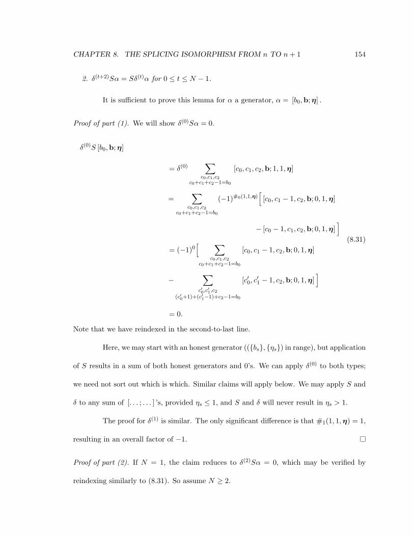
CHAPTER 8. THE SPLICING ISOMORPHISM FROM n TO n+ 1 154
2. δ(t+2)Sα = Sδ(t)α for 0 ≤ t ≤ N − 1.
It is sufficient to prove this lemma for α a generator, α = [b0,b; η] .
Proof of part (1). We will show δ(0)Sα = 0.
δ(0)S [b0,b; η]
= δ(0)∑
c0,c1,c2c0+c1+c2−1=b0
[c0, c1, c2,b; 1, 1,η]
=∑
c0,c1,c2c0+c1+c2−1=b0
(−1)#0(1,1,η)[
[c0, c1 − 1, c2,b; 0, 1,η]
− [c0 − 1, c1, c2,b; 0, 1,η]]
= (−1)0[ ∑
c0,c1,c2c0+c1+c2−1=b0
[c0, c1 − 1, c2,b; 0, 1,η]
−∑
c′0,c′1,c2
(c′0+1)+(c′1−1)+c2−1=b0
[c′0, c′1 − 1, c2,b; 0, 1,η]
]
= 0.
(8.31)
Note that we have reindexed in the second-to-last line.
Here, we may start with an honest generator (({bs}, {ηs}) in range), but application
of S results in a sum of both honest generators and 0’s. We can apply δ(0) to both types;
we need not sort out which is which. Similar claims will apply below. We may apply S and
δ to any sum of [. . . ; . . . ] ’s, provided ηs ≤ 1, and S and δ will never result in ηs > 1.
The proof for δ(1) is similar. The only significant difference is that #1(1, 1,η) = 1,
resulting in an overall factor of −1.
Proof of part (2). If N = 1, the claim reduces to δ(2)Sα = 0, which may be verified by
reindexing similarly to (8.31). So assume N ≥ 2.
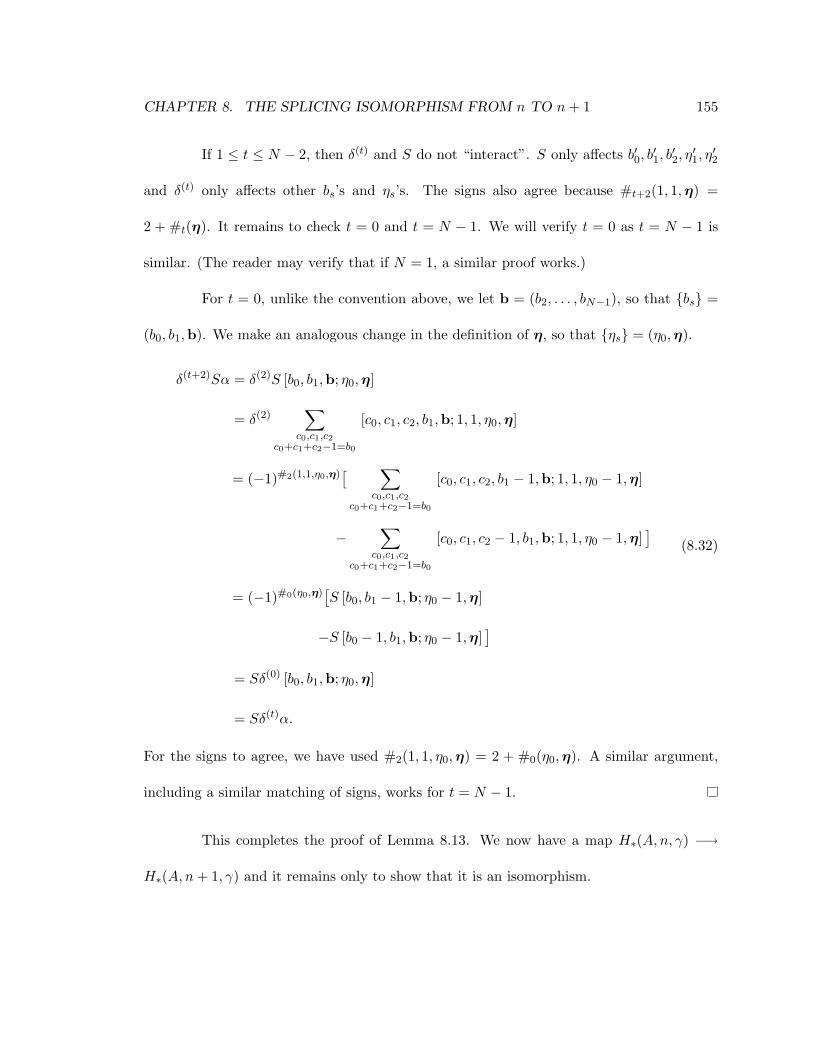
CHAPTER 8. THE SPLICING ISOMORPHISM FROM n TO n+ 1 155
If 1 ≤ t ≤ N − 2, then δ(t) and S do not “interact”. S only affects b′0, b′1, b′2, η′1, η′2
and δ(t) only affects other bs’s and ηs’s. The signs also agree because #t+2(1, 1,η) =
2 + #t(η). It remains to check t = 0 and t = N − 1. We will verify t = 0 as t = N − 1 is
similar. (The reader may verify that if N = 1, a similar proof works.)
For t = 0, unlike the convention above, we let b = (b2, . . . , bN−1), so that {bs} =
(b0, b1,b). We make an analogous change in the definition of η, so that {ηs} = (η0,η).
δ(t+2)Sα = δ(2)S [b0, b1,b; η0,η]
= δ(2)∑
c0,c1,c2c0+c1+c2−1=b0
[c0, c1, c2, b1,b; 1, 1, η0,η]
= (−1)#2(1,1,η0,η)[ ∑
c0,c1,c2c0+c1+c2−1=b0
[c0, c1, c2, b1 − 1,b; 1, 1, η0 − 1,η]
−∑
c0,c1,c2c0+c1+c2−1=b0
[c0, c1, c2 − 1, b1,b; 1, 1, η0 − 1,η]]
= (−1)#0(η0,η)[S [b0, b1 − 1,b; η0 − 1,η]
−S [b0 − 1, b1,b; η0 − 1,η]]
= Sδ(0) [b0, b1,b; η0,η]
= Sδ(t)α.
(8.32)
For the signs to agree, we have used #2(1, 1, η0,η) = 2 + #0(η0,η). A similar argument,
including a similar matching of signs, works for t = N − 1.
This completes the proof of Lemma 8.13. We now have a map H∗(A,n, γ) −→
H∗(A,n+ 1, γ) and it remains only to show that it is an isomorphism.
CHAPTER 8. THE SPLICING ISOMORPHISM FROM n TO n+ 1 156
8.4 S induces an isomorphism
In this section, we will show that S induces an isomorphism on homology, complet-
ing the proof of Theorem 8.1 and completing the calculation of H∗(A,n, γ). The plan is to
define filtrations on Cflat∗ (B(n)
∞ ) and Cflat∗ (B(n+1)
∞ ) compatible with S and consider the spec-
tral sequences, nE∗∗,∗ and n+1E∗∗,∗, of these filtered complexes. S will induce an isomorphism
on the E1∗,∗ sheets of the spectral sequences, and therefore an isomorphism on homology.
Definition 8.15. Given a (B(n)∞ , π/2)-flattened generator [b0, b1; η0, η1] , let
µ( [b0, b1; η0, η1] ) = 2N−1∑s=0
bs. (8.33)
Given a (B(n+1)∞ , π/2)-flattened generator [{b′s}; {η′s}] , let
µ′( [{b′s}; {η′s}] ) = b′0 + b′2 + 2N+1∑s=3
b′s. (8.34)
The crucial property of µ is that µ strictly decreases when we round a flattened
generator; whereas µ′ strictly decreases under rounding at any vertex except b′1.
The functions µ and µ′ define gradings on Cflat∗ (B(n)
∞ ,Θ0) and Cflat∗ (B(n+1)
∞ ,Θ0).
(They are gradings over Z. Recall that the usual grading, the ∗ in C∗, is over the Z-torsor
Z.) From the gradings, we may build increasing filtrations, denoted by FpCflat∗ (B(n)
∞ ,Θ0)
and FpCflat∗ (B(n+1)
∞ ,Θ0), making those chain complexes into filtered chain complexes.
The differentials on the two complexes respect the filtrations. Thus, we have two
spectral sequences.
Lemma 8.16. Suppose B∞ is an (A,n, γ)-strip, and i ∈ Z. Then there exists Xi > 0 such
that, for any (B∞, π/2)-flattened generator [{bs}; {ηs}] with I( [{bs}; {ηs}] ) = i, we have
|X(psbs)| ≤ Xi for s ∈ {0, . . . , N − 1}.

CHAPTER 8. THE SPLICING ISOMORPHISM FROM n TO n+ 1 157
Proof. Essentially the same proof as Lemma 6.12.
It follows that, for a given i ∈ Z, there are upper and lower bounds on b0, . . . , bN−1
of flattened generators with index i. Therefore, there are upper and lower bounds on
µ( [{bs}; {ηs}] ), and similarly for µ′. Thus the spectral sequences converge.
Lemma 8.17. S respects the filtrations.
Proof. We have µ( [b0,b; η] ) = 2b0 +∑N−1
s=1 bs and
µ′(S [b0,b; η] ) = c0 + c2 + 2N−1∑s=1
bs. (8.35)
Recall that c0, c2 ≤ b0 in any nonzero summand of S. Thus µ′(Sα) ≤ µ(α).
Thus we have a morphism of spectral sequences.
To prove an isomorphism on homology, it is sufficient to show, for some r, that
the map Er,flat∗,∗ → Er∗,∗ is an isomorphism. We will use r = 1.
Definition 8.18. Let C∗(b′0, b′2) be the chain complex generated by “truncated flattened
generators” defined on [Θ0,Θ2] with underlying path Λ′ satisfying Λ′(Θ0) = p′0b′0and Λ′(Θ2) =
p′2b′2. By truncated flattened generators, we mean that Λ′ satisfies the usual maximality con-
dition, and is labeled according to ‘E’ or ‘H’, on [Θ0,Θ1] and on [Θ1,Θ2].
The complex C∗(b′0, b′2) is isomorphic to the analogous complex in the proof of [5,
Proposition 7.5]. Its homology is 0 if b′0 6= b′2 and Z if b′0 = b′2. Let HHb′0denote the
truncated flattened generator with −b′1 = b′0 − 1 and b′2 = b′0, and with both labels ‘H’.
Then H∗(b′0, b′0) is generated by HHb′0
.
Given {bs}, we abbreviate Λ{bs}|[Θs,Θs+1] as Λs. Given {b′s}, define Λ′s similarly.
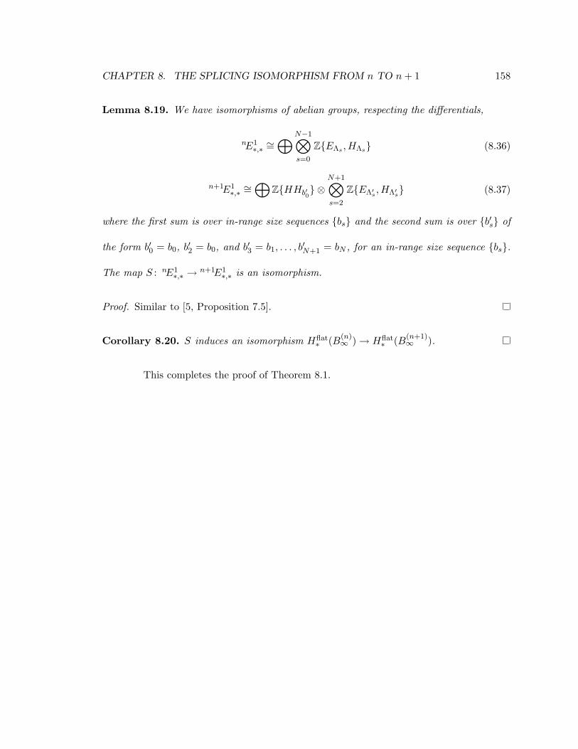
CHAPTER 8. THE SPLICING ISOMORPHISM FROM n TO n+ 1 158
Lemma 8.19. We have isomorphisms of abelian groups, respecting the differentials,
nE1∗,∗∼=⊕N−1⊗
s=0
Z{EΛs , HΛs} (8.36)
n+1E1∗,∗∼=⊕
Z{HHb′0} ⊗
N+1⊗s=2
Z{EΛ′s , HΛ′s} (8.37)
where the first sum is over in-range size sequences {bs} and the second sum is over {b′s} of
the form b′0 = b0, b′2 = b0, and b′3 = b1, . . . , b′N+1 = bN , for an in-range size sequence {bs}.
The map S : nE1∗,∗ → n+1E1
∗,∗ is an isomorphism.
Proof. Similar to [5, Proposition 7.5].
Corollary 8.20. S induces an isomorphism Hflat∗ (B(n)
∞ )→ Hflat∗ (B(n+1)
∞ ).
This completes the proof of Theorem 8.1.

159
Appendix A
Combinatorial homology and ECH
The goal of this appendix is to prove that Hi(A,n, γ) ∼= ECH∗(YA, λn,Γ), i.e., the
combinatorially defined homology is isomorphic to the analytically defined homology. The
argument is very similar to the T 3 case [5, §10-11], and we mostly describe the differences.
A.1 Periodic paths and Morse-Bott orbit sets
Throughout this appendix, we will just say Reeb orbit for a closed embedded Reeb
orbit, and Reeb orbit family for a component of the space of embedded closed Reeb orbits
of (YA, λn).
Definition A.1. A Morse-Bott orbit set of (YA, λn,Γ) is a finite set of pairs α = {(αi,mi)}
where each αi is a Reeb orbit family and each mi is a positive integer, and the homology
classes of the Reeb orbits satisfy∑
imi[αi] = Γ.
Our first step is to show that a Morse-Bott orbit set is equivalent to a collection
of angles and integer vectors; this is the data of a periodic path, modulo a Z2-translation
APPENDIX A. COMBINATORIAL HOMOLOGY AND ECH 160
ambiguity.
Lemma A.2. A Morse-Bott orbit set of (YA, λn,Γ) is equivalent to a discrete fA,n-invariant
set Ang ⊂ R together with a function−−−→Edge : Ang→ Z2 \ {0} satisfying
−−−→Edge(fA,n(θ)) = A(
−−−→Edge(θ)) (A.1)∑
θ∈Ang∩(θ0,fA,n(θ0))
−−−→Edge(θ) ∈ Γ. (A.2)
Here, the choice of θ0 ∈ R \ Ang does not matter. By “equivalent” we mean we
construct a bijection.
Proof. A Reeb orbit family is equivalent to an element [θ] ∈ R/fA,n, the image of θ ∈ R
with tan θ ∈ Q ∪ {∞}, because the (closed) Reeb orbits in YA form S1-families in the
corresponding fibers of the bundle YA, a bundle over R/fA,n. Thus a finite set of Reeb orbit
families is equivalent to a discrete fA,n-invariant set.
Given θ ∈ R with tan θ ∈ Q ∪ {∞}, let(xθyθ
)∈ Z2 \ {0} be the unique positive
multiple of(
cos θsin θ
)with gcd(xθ, yθ) = 1. Given (αi,mi) with αi corresponding to [θi], let
−−−→Edge(θi) = mi
(xθiyθi
).
Lemma A.3. A Morse-Bott orbit set of (YA, λn,Γ) is equivalent to an (A,n, γ)-periodic
path.
Proof. A periodic path Λ yields Ang and−−−→Edge as in Lemma A.2. For an angle θ0 at which
Λ has no edge,
Λ(fA,n(θ0)) = AΛ(θ0) + γ (A.3)
Λ(fA,n(θ0))− Λ(θ0) =∑
θ∈Ang(Λ)∩(θ0,fA,n(θ0))
−−−−−−→EdgeΛ(θ), (A.4)

APPENDIX A. COMBINATORIAL HOMOLOGY AND ECH 161
where−−−−−−→EdgeΛ(θ) is the vector from the beginning to the end of that edge. It follows that
Λ(θ0) = (A− 1)−1
−γ +∑
θ∈Ang(Λ)∩(θ0,fA,n(θ0))
−−−−−−→EdgeΛ(θ)
. (A.5)
Thus we may obtain Λ uniquely, given Ang and−−−→Edge. As we move θ0 past some θ′, observe
that Λ defined by (A.5) jumps by−−−→Edge(θ′).
It follows that we may think of a labeled periodic path as a Morse-Bott orbit set
with each Reeb orbit family αi labeled ‘e’ or ‘h’ (and with an ordering on the ‘h’ labels).
We may perturb the contact form in a neighborhood of the T 2-fiber containing αi, replacing
the family of degenerate Reeb orbits with one elliptic and one hyperbolic Reeb orbit. Then:
• (αi,mi) with an ‘e’ label corresponds to the elliptic Reeb orbit with multiplicity mi.
• (αi,mi) with an ‘h’ label corresponds to the elliptic Reeb orbit with multiplicity mi−1,
together with the hyperbolic Reeb orbit with multiplicity 1.
Given a positive real L, we may perform the above small perturbations simulta-
neously on all fibers containing Reeb orbits with symplectic action less than L, obtaining a
contact form λ<L. The subcomplex of the embedded contact homology chain complex for
(YA, λ<L,Γ) generated by collections α of Reeb orbits with the symplectic action of α less
than L is isomorphic (as an abelian group) to a subcomplex of C∗(A,n, γ), and a direct
limit yields a chain complex isomorphic (as an abelian group) to C∗(A,n, γ).
The combinatorially defined index using SizeR from §3.6 is a straightforward gen-
eralization from the T 3 case, and agrees with the analytically defined index.
APPENDIX A. COMBINATORIAL HOMOLOGY AND ECH 162
A.2 The differential
We will not prove that the combinatorial and analytical differentials agree; we will
prove a weaker statement sufficient to show that the homologies are isomorphic. Denote
the combinatorial differential by δcom and the analytical differential by δan.
Definition A.4. If a labeled periodic path (Λ, `, o) has ‘h’-labeled edges at θ1, θ2, and θ3
(with no edges in (θ1, θ2) ∪ (θ2, θ3)), we say (Λ′, `′, o′) is obtained from (Λ, `, o) by double
rounding if
1. Λ′ is obtained from Λ by rounding at (θ1, θ2) and at (θ2, θ3), i.e., Λ′ = Λ \ (θ1, θ2) \
(θ2, θ3).
2. The labeling `′ has only ‘e’ labels in [θ1, θ3].
3. Outside of [θ1, θ3] and its periodic images (fA,n)k[θ1, θ3], the labeling `′ and its ordering
o′ are the restriction of ` and o.
Lemma A.5. Suppose α and β are labeled periodic paths.
1. If 〈δanα, β〉 6= 0, then 〈δcomα, β〉 6= 0 or β is obtained from α by double rounding.
2. If 〈δcomα, β〉 6= 0, then 〈δcomα, β〉 = 〈δanα, β〉.
The proof is the same as in the T 3 case, because the situation in YA is locally the
same as T 3.
Lemma A.6. The number of ‘h’ labels of a generator of H∗(A,n, γ) is either N or N − 1.

APPENDIX A. COMBINATORIAL HOMOLOGY AND ECH 163
Proof. For the N = 1 case, see the proof of Theorem 5.36. For the N = 2 case, see the
explicit generators given at the end of Chapter 7. For N > 2, each application of the
splicing isomorphism increases both N and #h by 2.
The spectral sequence argument given in [4] now shows that the chain complex
with δan has the same homology as the chain complex with δcom. That argument requires
the number of ‘h’ labels of generators of the homology H∗(A,n, γ) to lie within a range of
3, and #h lies within a range of 2.
164
Bibliography
[1] Y. Eliashberg, A. Givental, and H. Hofer. Introduction to symplectic field theory.
Geom. Funct. Anal., (Special Volume, Part II):560–673, 2000. GAFA 2000 (Tel Aviv,
1999).
[2] Allen Hatcher. Algebraic Topology. Cambridge University Press, 1st edition, 2001.
[3] M. Hutchings. An index inequality for embedded pseudoholomorphic curves in sym-
plectizations. Journal of the European Mathematical Society, 4(4):313–361, 2002.
[4] Michael Hutchings and Michael Sullivan. The periodic Floer homology of a Dehn twist.
Algebr. Geom. Topol., 5:301–354 (electronic), 2005.
[5] Michael Hutchings and Michael Sullivan. Rounding corners of polygons and the em-
bedded contact homology of T 3. Geom. Topol., 10:169–266 (electronic), 2006.
[6] Michael Hutchings and Clifford Henry Taubes. Gluing pseu-
doholomorphic curves along branched covered cylinders I, 2007.
http://www.citebase.org/abstract?id=oai:arXiv.org:math/0701300.
BIBLIOGRAPHY 165
[7] P. B. Kronheimer and T. Mrowka. Monopoles and three-manifolds. Cambridge Uni-
versity Press, to appear.
[8] Peter Ozsvath and Zoltan Szabo. Holomorphic disks and three-manifold invariants:
properties and applications. Ann. of Math. (2), 159(3):1159–1245, 2004.
[9] Peter Ozsvath and Zoltan Szabo. Holomorphic disks and topological invariants for
closed three-manifolds. Ann. of Math. (2), 159(3):1027–1158, 2004.
[10] Clifford Henry Taubes. The Seiberg-Witten and Gromov invariants. Math. Res. Lett.,
2(2):221–238, 1995.
[11] Clifford Henry Taubes. Seiberg Witten and Gromov invariants for symplectic 4-
manifolds, volume 2 of First International Press Lecture Series. International Press,
Somerville, MA, 2000. Edited by Richard Wentworth.
[12] Clifford Henry Taubes. The Seiberg-Witten equations and the Weinstein conjecture,
2006. arXiv:math/0611007v3 [math.SG].
[13] Clifford Henry Taubes, 2007. Lecture at Yashafest.