emmanuel n. saridakis and joel m. weller- a quintom scenario with mixed kinetic terms

8/3/2019 Emmanuel N. Saridakis and Joel M. Weller- A Quintom scenario with mixed kinetic terms

http://slidepdf.com/reader/full/emmanuel-n-saridakis-and-joel-m-weller-a-quintom-scenario-with-mixed-kinetic 1/11

a r X i v : 0 9 1 2

. 5 3 0 4 v 2

[ h e p - t h ]

2 1 J u n 2 0 1 0

A Quintom scenario with mixed kinetic terms

Emmanuel N. Saridakis1, ∗ and Joel M. Weller2, †1College of Mathematics and Physics, Chongqing University of Posts and Telecommunications,

Chongqing, 400065, P.R. China 2 Department of Applied Mathematics, University of Sheffield,

Hounsfield Road, Sheffield S3 7RH, United Kingdom

We examine an extension of the quintom scenario of dark energy, in which a canonical scalar fieldand a phantom field are coupled through a kinetic interaction. We p erform a phase space analysisand show that the kinetic coupling gives rise to novel cosmological behaviour. In particular, weobtain both quintessence-like and phantom-like late-time solutions, as well as solutions that crossthe phantom divide during the evolution of the Universe.

PACS numbers: 98.80.-k, 95.36.+x

I. INTRODUCTION

According to independent observational data, includ-ing measurements of type Ia supernovae [1], the Wilkin-son Microwave Anisotropy Probe [2], the Sloan Digital

Sky Survey [3], and X-ray observations [4], the Universeis undergoing a phase of accelerated expansion. Althoughthe cosmological constant seems to be a simple and eco-nomic way to explain this behaviour [5], the extreme de-gree of fine-tuning associated with this means that it isattractive to consider other dark energy candidates. Thedynamical nature of dark energy, at least at an effectivelevel, can originate from various fields, such as a canon-ical scalar field (quintessence) [6] or a phantom field [7](i.e. a scalar field with negative kinetic terms). Anotherpossibility of considerable interest is the quintom scenario[8–10], in which the acceleration is driven by a combina-tion of quintessence and phantom fields. The quintom

paradigm has the advantage of allowing the dark energyequation-of-state (EOS) parameter (wDE) to cross thephantom divide during the evolution of the Universe, anintriguing possibility for which there is observational ev-idence from a variety of sources (see [10] for a review).

The aforementioned models offer a satisfactory descrip-tion of the behaviour of dark energy and its observablefeatures. However, the dynamical nature of dark energyin these scenarios leads to the “coincidence” problem,which many authors have sought to resolve by consider-ing a coupling between dark energy and the other com-ponents of the Universe. Thus, various forms of interact-ing dark energy models have been constructed, including

coupled quintessence [11] and interacting phantom mod-els [12]. Similarly, the dynamical nature of dark energymakes it difficult to fulfil the observational requirement,wDE ≈ −1 [13], which has led to the introduction of ad-ditional scalar fields. Inspired by similar multi-field infla-tion [14] and assisted inflation constructions [15], various

∗Electronic address: [email protected]†Electronic address: [email protected]

forms of assisted dark energy models have been consid-ered [16, 17].

One generalised class of the multi-field quintessencescenario allows for a mixing of the fields’ kinetic terms[18] (see also [19]). Mixed kinetic terms appear also inthe non-trivial scalar field models based on string theory

constructions, studied in the framework of generalisedmulti-field inflation [20].

In the present work we aim to combine the advan-tages of the quintom scenario with those of assistedquintessence with mixed kinetic terms. Thus, we con-struct a quintom model in which the kinetic terms of thecanonical and the phantom fields are mixed. Indeed, aswe see, the model exhibits features characteristic of bothquintessence and phantom models.

The plan of the work is as follows. In Sec. II weconstruct the quintom cosmological scenario with mixedkinetic terms and present the formalism for its transfor-mation into an autonomous dynamical system. In Sec.

III we perform the phase-space stability analysis and inSec. IV we discuss the cosmological implications of theresults. Finally, our conclusions are presented in Sec. V.

II. QUINTOM SCENARIO WITH MIXED

KINETIC TERMS

Let us construct the quintom cosmological scenariowith mixed kinetic terms. Throughout the work we con-sider a flat Robertson-Walker metric:

ds2 = dt2 − a2(t)dx2, (1)

with a the scale factor.We consider a model consisting of a canonical scalar

field φ, a phantom field σ and a mixed kinetic term pro-portional to the parameter α. Thus, the action, in unitswhere 8πG = 1 reads:

S =

d4x

√−g

R

2− 1

2gµν∂ µφ∂ νφ +

1

2gµν∂ µσ∂ νσ−

−α

2gµν∂ µφ∂ νσ + V φ(φ) + V σ(σ)

+ S M , (2)

http://arxiv.org/abs/0912.5304v2


































mailto:[email protected]







2

with V φ(φ) and V σ(σ) the corresponding field poten-tials, and S M the action for the matter (dark plus bary-onic) component of the Universe. We assume that thematter is described by a perfect fluid with energy den-sity ρM , pressure pM and barotropic index γ . Thus,

pM = (γ − 1)ρM and the matter equation-of-state pa-rameter is wM = γ − 1. Varying the action with respectto the metric yields the Friedmann equations

H 2 =1

3

1

2φ2 − 1

2σ2 +

α

2φσ +

+V φ(φ) + V σ(σ) + ρM

, (3)

H +3

2H 2 = −1

2

1

2φ2 − 1

2σ2 +

α

2φσ −

−V φ(φ) − V σ(σ) + pM

, (4)

while the evolution equations for the two fields read

φ + 3H φ +∂V φ∂φ

+α

2

∂V σ∂σ 1 +

α2

4 −1

= 0, (5)

σ + 3H σ +

−∂V σ

∂σ+

α

2

∂V φ∂φ

1 +

α2

4

−1

= 0. (6)

In quintom scenarios the dark energy is attributed tothe combination of the two scalar fields. In the case athand, from the Friedmann equations (3),(4) we straight-forwardly read the dark energy density and pressure as

ρDE =1

2φ2 − 1

2σ2 +

α

2φσ + V φ(φ) + V σ(σ) (7)

pDE =1

2φ2 − 1

2σ2 +

α

2φσ − V φ(φ) − V σ(σ), (8)

and thus for the dark energy equation-of-state parameterwe obtain

wDE ≡ pDEρDE

=12 φ2 − 1

2 σ2 + α2 φσ − V φ(φ) − V σ(σ)

12 φ2 − 1

2 σ2 + α2 φσ + V φ(φ) + V σ(σ)

.

(9)Finally, using (7),(8) and (5),(6), we can easily acquirethe dark energy evolution equation in fluid terms, whichtakes the expected form

ρDE + 3H (ρDE + pDE) = 0. (10)

We mention that in the case α = 0 the above scenariocoincides with the usual quintom one [9].

III. PHASE-SPACE ANALYSIS

In order to perform the phase-space and stability anal-ysis of the quintom model at hand, we have to trans-form the aforementioned dynamical system into its au-tonomous form [21–23]. This can be achieved by intro-

ducing the auxiliary variables:

xφ =φ√6H

, xσ =σ√6H

,

yφ =

V φ(φ)√

3H , yσ =

V σ(σ)√

3H , (11)

together with N = ln a. It is easy to see that for everyquantity F we acquire F = H dF

dN . Using these variables,

from (7) we can calculate the dark energy density param-eter,

ΩDE ≡ ρDE3H 2

= x2φ − x2

σ + αxφxσ + y2φ + y2σ, (12)

and from (9) the dark energy equation-of-state parame-ter,

wDE =x2φ − x2σ + αxφxσ − y2φ − y2σ

x2φ

−x2σ + αxφxσ + y2φ + y2σ

. (13)

The final step is the consideration of specific poten-tial forms. Following works on assisted quintessence [17]and assisted inflation [15] scenarios, together with vari-ous other cosmological models [21, 23, 24], we considerexponential potentials of the form,

V φ(φ) = e−λφ, V σ(σ) = e−µσ. (14)

Note that equivalently, but more generally, we could con-

sider potentials satisfying λ = − 1κV (φ)

∂V (φ)∂φ

≈ const,

µ =

−1

κV (σ)∂V (σ)∂σ

≈const (for example this relation is

valid for arbitrary but nearly flat potentials [25]). Fi-nally, without loss of generality, in this work we considerλ and µ to be positive, since the negative case alters onlythe direction towards which the fields roll, and can al-ways be transformed into the positive case by changingthe signs of the fields themselves.

Let us now perform the phase-space analysis of themodel. In general, having transformed the cosmologicalsystem into its autonomous form X′ = f(X), where Xis the column vector constituted by the auxiliary vari-ables, f(X) the corresponding column vector of the au-tonomous equations, and prime denotes a derivative withrespect to N = ln a, the critical points Xc are extracted

satisfying X′ = 0. In order to determine the stabilityproperties of these critical points we expand around Xc,setting X = Xc + U with U the perturbations of thevariables considered as a column vector. Up to first or-der we acquire U′ = Q ·U, where the matrix Q containsthe coefficients of the perturbation equations. Thus, foreach critical point, the eigenvalues of Q determine itstype and stability.

Following this method and using the auxiliary variables(11), the cosmological equations of motion (3), (4), (5)



3

and (6) become

x′φ = −3xφ +

3

2

1 +

α2

4

−1 λy2φ +

α

2µy2σ

+ xφT,

x′σ = −3xσ −

3

2

1 +

α2

4

−1 µy2σ − α

2λy2φ

+ xσT,

y′φ = − 3

2 λxφyφ + yφT,

y′σ = −

3

2µxσyσ + yσT, (15)

where

T =3

2

2x2φ − 2x2

σ + 2αxφxσ

+γ (1 − x2φ + x2σ − αxφxσ − y2φ − y2σ)

. (16)

The critical points (xφc, xσc, yφc, yσc) of the au-tonomous system (15) are obtained by setting the lefthand sides of the equations to zero. The real and phys-

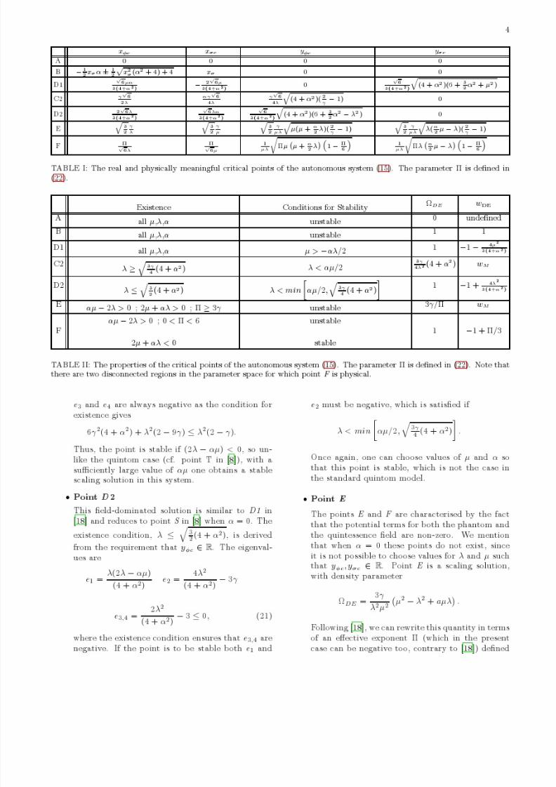
ically meaningful (i.e. corresponding to yφ, yσ > 0, and0 ≤ ΩDE ≤ 1) points are presented in Table I.

The 4×4 matrix Q of the linearised perturbation equa-tions of the system (15) is shown in the Appendix. Thus,for each critical point of Table I we examine the sign of the real part of the eigenvalues of Q to determine thetype and stability of the point. In Table II we presentthe results of the stability analysis. In addition, for eachcritical point we calculate the values of ΩDE [given by(12)] and of wDE [given by (13)]. Finally, we mentionthat the labelling of the critical points follows the con-vention used in [18]. That is, since in a two-field systemthere are critical points in which the potential term of one

of the fields is zero, the connection between these pointsis made more explicit. For instance, in the points D1 andD2 (for which ΩDE = 1) only one of the fields’ potentialterms contributes to the energy density. Note that in thismodel (unlike that in [18]) the solution satisfying X′ = 0with yφ = 0 corresponding to C1 is unphysical.

The stability of the critical points can be summarisedas follows:

• Point A

This is a trivial solution, corresponding to the fluiddominated point F in [8], where the kinetic andpotential components of both the phantom and thequintessence fields are negligible. It exists for allvalues of α, λ and µ. The eigenvalues are

e1 = e2 = 32

γ > 0,

e3 = e4 = − 32 (2 − γ ) < 0, (17)

so this is a saddle point.

• Point B

The two points indicated by the ± are similar topoint B in [18]. When α = 0 (point K in [8]), there

is a continuous locus of points that describes a hy-perbola in the (xφ, xσ) plane. When α = 0 the lo-cus still describes a hyperbola, but the asymptotesare no longer orthogonal. The eigenvalues are

e1 = 3(2 − γ ) > 0,

e2 = 0,

e3 = 3

−5√ 6

4µxσ

+ 3√ 64 λ

− 1

2xσα ± 12

x2σ(α2 + 4) + 4

,

e4 = 3 + 3√ 6

4µxσ

− 5√ 6

4 λ− 1

2xσα ± 12

x2σ(α2 + 4) + 4

, (18)

where the ± in e3 and e4 corresponds to the par-ticular solution considered. e1 is positive, thereforethe point is unstable.

• Point D 1

This takes a similar form to point D1 in [18]. (Theyσ value in the solution corresponding to C1 in [18]

has a factor of (4 + α2)(1−

2/γ ) so there are noreal values of α for which the point exists.) In thestandard quintom case (α = 0), D1 is a phantom-dominated point (point P in the notation of [8]).In that case, as in the present one, the term underthe square root in yσc is positive and ΩDE = 1,so the point exists for all values of the parameters.However, in the case at hand, the eigenvalues read

e1,2 = − 2µ2

(4 + α2)− 3 ≤ 0,

e3 = − 4µ2

(4 + α2)− 3γ ≤ 0,

e4 = −µ(2µ + αλ)

(4 + α2) , (19)

so the point is stable only if (2µ + αλ) > 0, whichis trivially satisfied when α ≥ 0.

• Point C 2

The points C2 and D2 are similar to D1, in thatonly one of the fields’ potential energy contributesto the total energy density; in D1 this was thephantom field, while here it is the quintessenceone. This means that there is both a scaling so-lution (C2 ) and a field-dominated solution (D2 ),for which ΩDE = 1. The density parameter for C2 is ΩDE = 3γ

4λ2 (4 + α2), so the condition ΩDE

≤1

means that λ ≥

3γ4 (4 + α2) must be satisfied if

the point is to be physical. The eigenvalues are

e1 = − 32(2 − γ ) < 0,

e2 = 3γ4λ(2λ − αµ),

e3,4 = − 3(2−γ)4

×

1 ±

6γ 2(4 + α2) + λ2(2 − 9γ )

λ2(2 − γ )

. (20)



5

by

1

Π=

1

λ2− 1

µ2+

α

µλ, (22)

which leads to the existence condition Π ≥ 3γ .Note that, as µ, λ ≥ 0,

(αµ−

2λ) > 0⇒

(2µ + αλ) > 0. (23)

Thus, to ensure that yφc and yσc are real, one mustadditionally impose (αµ−2λ) > 0. The eigenvaluesare

e1,2 = − 34(2 − γ )

×

1 ±

24γ 2/Π + 2 − 9γ

(2 − γ )

, (24)

e3,4 = − 34(2 − γ )

× 1 ±

1 − 8γ (2µ + αλ)(2λ − αµ)

λµ(2−

γ )(4 + α2) . (25)

In terms of Π the existence condition reads 24γ2

Π +2 − 9γ ≤ (2 − γ ); substituting this into (24) leadsto e1,2 ≤ − 3

4(2 − γ )(1 ± 1) ≤ 0. However, lookingat the fraction under the square root in (25), weobserve that

1 − 8γ (2µ + αλ)(2λ − αµ)

λµ(2 − γ )(4 + α2)> 1.

Thus, either e3 or e4 must be positive, and thereforethe critical point is unstable.

• Point F In this (field-dominated) point we observe the pres-ence of square-root terms in yφc and yσc . Thus, forthese values to be real we require

Π

1 − Π

6

(2µ + αλ) > 0,

Π

1 − Π

6

(αµ − 2λ) > 0.

Using (22) and (23), and noting that

(2µ + αλ) < 0

⇒(αµ

−2λ) < 0, (26)

and

(2µ + αλ) < 0 ⇒ µ2 − λ2 + aµλ < 0

⇒ Π < 0, (27)

we conclude that there exist two possible cases:

(a) αµ − 2λ > 0; 0 < Π < 6, (28)

(b) 2µ + αλ < 0. (29)

The eigenvalues read

e1 = −3

1 − Π

6

,

e2 = Π − 3γ,

e3,4 = −3

2

1 − Π

6

× 1 ±

1 − 4Π3λµ

(2µ + αλ)(2λ − αµ)(4 + α2)

1 − Π

6

. (30)

In case (a),

1 − Π6

> 0, thus e1 < 0. However, in

a similar way to the analysis of point E , the termunder the square root in the expression for e3,4 isgreater than 1 so either e3 or e4 is positive and thepoint is unstable. In case (b), the term under thesquare root is less than 1 so e3,4 < 0. e2 < 0 is triv-

ially satisfied [using (27)] and, again,

1 − Π6

> 0,

therefore e1 < 0. Thus, the point is stable wheneverthe condition (29) is satisfied. Finally, we mentionthat this separation of the parameter space is a

novel feature of the scenario at hand, which is notpresent in the corresponding case of two canonicalfields [18].

The stability regions for the points are plotted in Fig.1. In the standard quintom case (α = 0), there is only onestable critical point that exists for all values of µ and λ,corresponding to the phantom point D1. In the case α <0 the parameter space is fractured, thus, although thereis a stable point with wDE < −1 at each parameter-spaceregion, the precise value of wDE for particular values of µ and λ depends on whether point D1 or F is stable. Inthe case where α > 0, the phantom dominated point D1

is always stable. It is interesting, however, that thereare also regions where C2 (a scaling solution) and D2 (aquintessence-dominated solution), each with wDE > −1,are stable. In these regions the initial conditions willdetermine the cosmological evolution.

As we have seen, point F exists in two disconnectedregions in the parameter space: a stable region whereα < 0 and an unstable region where α > 0. This can beunderstood as a fracture of the unstable regions in theparameter space, depicted in Fig. 2. In the standardquintom case, there are two overlapping regions corre-sponding to C2 and D2 . When αµ − 2λ > 0 the pointsE and F are present and encroach upon this region. Asone might expect, in both cases, when the exponent of

the quintessence field is large, the scaling solution doesexist (although it is not always stable).

IV. COSMOLOGICAL IMPLICATIONS

Having performed the complete phase-space analysis of the model, we can discuss the corresponding cosmologi-cal behaviour. A general remark is that the phenomenol-ogy is different from both the standard (α = 0) quintom



6

(a)

(b)

FIG. 1: The parameter space showing the stability of thecritical points for (a) α = −3 and (b) α = 3, with γ = 1. Thelight shaded area indicates the region where D1 is stable andthe dark shaded area indicates the region where F is stable.

There is a stable point with wDE < −1 at each region in theparameter space. The area marked in graph (b) indicates theregion where C2 and D2 are stable.

scenario [8, 9] and from the case of quintessence withmixed kinetic terms [18]. In particular, there are late-time solutions describing both quintessence and phantomdominated universes, with the crucial observable quan-tity being the dark energy equation-of-state parameter

FIG. 2: Regions in the parameter space where the criticalpoints exist but are unstable for α = 3 (with γ = 1).

wDE (which is greater than −1 in the former case andless than −1 in the latter).

The points A, B and E are unstable, and thus cannotbe late-time solutions of the Universe. A corresponds toa matter-dominated universe, while B represents a darkenergy-dominated one, with the stiff value wDE = 1. E isa scaling solution. Finally, in one of the two disconnectedareas in which F is physical, when αµ − 2λ > 0 and0 < Π < 6, which corresponds to wDE > −1, the point isalways unstable.

As usual, the stable critical points can be classified asfield-dominated (ΩDE = 1) or scaling solutions (wDE = 0in the presence of matter). Since these features are in-compatible with observations, we deduce that the late-time behaviour of the scenario considered here cannotprovide a satisfactory description of the Universe at thepresent time. However, the fact that dark energy hasonly recently begun to dominate the energy density, af-ter an extended matter-dominated era, suggests that theUniverse may have yet to reach an attractor solution. Inthis case, one can consider our Universe as evolving to-wards a field dominant attractor, although the problemwith initial conditions is still an issue [26].

In order to treat the coincidence problem one must ex-plain why the present dark energy and matter densityparameters are of the same order of magnitude. Alter-natively, one can ask why dark energy has only recentlybecome dynamically important, which is a problem of initial conditions. This can be alleviated if ρDE scaleswith the dominant matter component, as the discrep-ancy between the initial energy densities of the variouscomponents of the Universe does not have to be so large.

In contrast to the simple quintom scenario with α =



7

0, there is a stable scaling solution in this model, viz.point C2 , which is an extension of the unstable point Tin [8]. However, as the present model stands, there isno mechanism to effect a transition between the scalingregime and field-dominant solution without fine-tuningthe initial conditions.

Another novel feature of the extended quintom sce-nario is a stable field-dominated late-time solution with

wDE > −1 (point D2 ) which is characterised by the factthat the contribution of the potential of the phantom fieldto the energy density is zero. Like C2 , this is an extensionof an unstable point in the simple quintom scenario. Thedeviation from wDE = −1 is 4λ2/[3(4 + α2)] so one re-quires either the coupling to be large or the quintessencepotential to be sufficiently flat for this solution to becompatible with observations.

Let us make an important comment concerning C2

and D2 . As can be seen in Table I, both points havexσc > 0 in the regions in which they are stable (we con-sider positive potential exponents λ, µ > 0). However,since phantom fields generally do not roll down their po-

tential slopes, one would normally expect that in a sta-ble late-time solution, the rate of change of the phantomfield, that is xσc , should be negative (in a stationary solu-tion) or zero (in a static solution). Indeed, for the simplequintom case (α = 0) we do obtain xσc = 0. Interestinglyenough, the positive coupling of the kinetic terms of thetwo fields makes the quintessence field drag the phantomfield down its potential (i.e. the opposite to “normal”phantom behaviour). This possibility is a novel featureof the present scenario.

The point D1 is the analogue of D2 and is stable forthe larger part of the parameter space (it is always stablefor α ≥ 0, while for α < 0 it can still be stable for µ >

−αλ/2). w

DEdepends only on the values of µ and α and

approaches −1 if the potential is flat or the coupling islarge, in a similar manner to the quintessence-dominatedpoint, D2 . Furthermore, it is interesting to note in thiscase there is a situation similar to the one described in theprevious paragraph. In particular, for α < 0 we observethat xφc < 0, so, contrary to expectations, there is astable late-time solution where the quintessence field rollsup its potential slope. Again, this is due to the couplingof the kinetic terms: the phantom field feeds the upwardrolling of the quintessence field.

From the discussion of the above two paragraphs wededuce that the kinetic coupling leads to new stable so-lutions. Additionally, it could lead to a very interesting

evolution towards these late-time solutions. In particu-lar, if the kinetic terms are initially small, the effect of the coupling is downgraded, and the fields can move awayfrom these stable points. With the increase of their ki-netic energies, the coupling becomes more important andthey will start to move towards them.

When point D1 is unstable, the critical point F , in oneof the two disconnected areas for which it is physical,viz. 2µ + αλ < 0, is stable. It corresponds to a universecompletely dominated by dark energy, behaving like a

phantom, with the EOS determined by the parameter Π.In this case, the quintessence and phantom fields combineto give a solution with wDE < −1. This is the analogueof point F in [18] and, like the unstable point E , does notexist in the standard quintom case.

0 1 2 3 4 5 6 7 8 9−1.3

−1.2

−1.1

−1

−0.9

−0.8

−0.7

−0.6

N

w D E

(a)

0 1 2 3 4 5 6 7 8 9−1.8

−1.6

−1.4

−1.2

−1

−0.8

−0.6

−0.4

−0.2

0

0.2

N

w D E

(b)

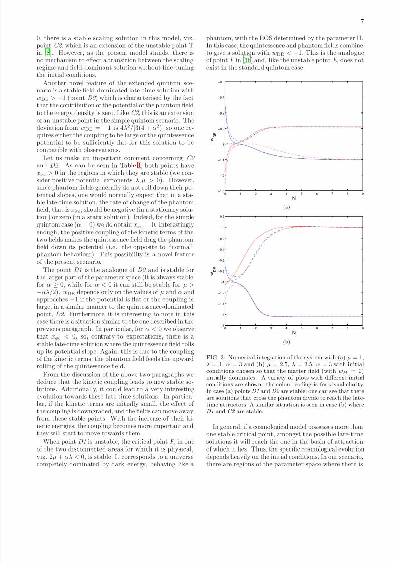
FIG. 3: Numerical integration of the system with (a) µ = 1,λ = 1, α = 3 and (b) µ = 2.5, λ = 3.5, α = 3 with initialconditions chosen so that the matter field (with wM = 0)initially dominates. A variety of plots with different initialconditions are shown: the colour-coding is for visual clarity.In case (a) points D1 and D2 are stable; one can see that thereare solutions that cross the phantom divide to reach the late-time attractors. A similar situation is seen in case (b) whereD1 and C2 are stable.

In general, if a cosmological model possesses more thanone stable critical point, amongst the possible late-timesolutions it will reach the one in the basin of attractionof which it lies. Thus, the specific cosmological evolutiondepends heavily on the initial conditions. In our scenario,there are regions of the parameter space where there is



8

both a stable quintessence-like and a stable phantom-like critical point. Therefore, the EOS can always re-main in the quintessence or the phantom regime, crossthe phantom divide from below to above, or cross thephantom divide from above to below, with the last possi-bility mildly favoured by observations. It must be noted,however, that in the absence of constraints on the cou-pling α and the potential exponents, a late-time solution

with wDE < −1 seems likely as there is a stable phantom-like critical point in every region of the parameter space.This fact is an advantage of the model.

As we know, the standard quintom model [8–10] ex-hibits only one (phantom-like) stable late-time solution,and in order to acquire the simultaneous existence of one quintessence and one phantom stable late-time so-lutions, one has to extend to significantly generalizedquintom models [24]. On the other hand, the model athand presents this behavior more economically. Further-more, note that the extended scenario of this work ex-hibits a novel situation, viz. the presence of more thanone stable attractor (points C2 and D2 ) corresponding to

quintessence-like solutions. Thus, according to the spe-cific parameter values, and for suitable initial conditions,the late-time behaviour of the Universe can be describedby one of the quintessence-like states, with D2 possessinga more physical EOS compared to C2 (see Table II).

In order to present the late-time behaviour transpar-ently, in Fig. 3 we depict the results of a numerical in-tegration for two choices of parameter values. In graph(a) the phantom stable point is D1 and the quintessenceone is D2 , while in graph (b) the phantom stable pointis also D1 but the quintessence one is C2. If the systemavoids the stable phantom solution, it will tend towardone of the two quintessence-like solutions, depending onthe values of the parameters, α, µ and λ.

We have to mention that for a particular subclass of evolutionary trajectories, depending on the parametervalues and initial conditions, the dark energy EOS be-comes infinite at a finite time t∗. However, this diver-gence in wDE is not accompanied by a divergence in thescale factor, its time-derivative or in the dark energy den-sity and pressure, but is an expected result arising fromthe nullification of ρDE , possible in all phantom models.Thus, technically, it does not correspond to the Big Ripdiscussed in the literature [27], but rather to the new sin-gularity family discussed in [28]. One could consider onlythose models in which the total energy density remainspositive (where the potential is sufficiently positive or the

phantom kinetic energy not too large), to avoid the cor-responding energy condition violation. Finally, note thatwhile a negative coupling value α facilitates the nullifica-tion of ρDE , a positive α obstructs it.

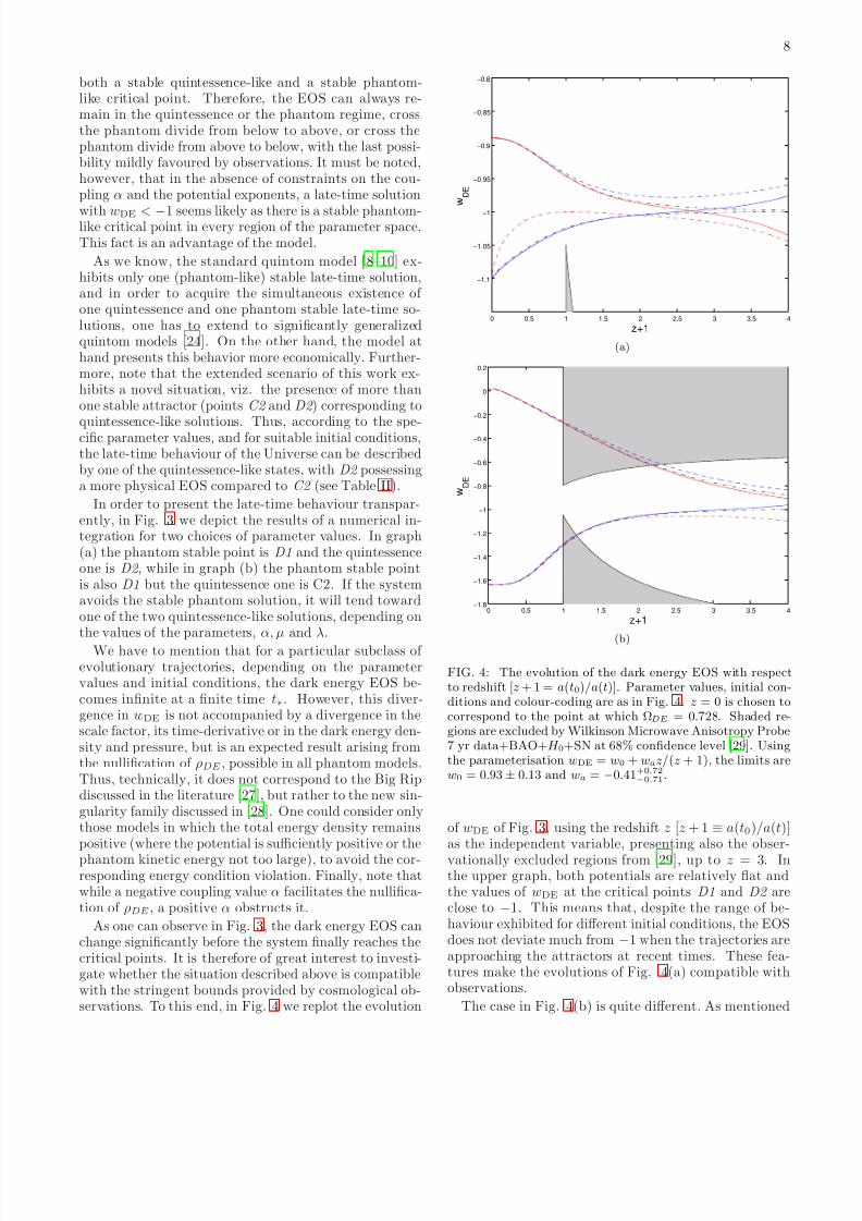
As one can observe in Fig. 3, the dark energy EOS canchange significantly before the system finally reaches thecritical points. It is therefore of great interest to investi-gate whether the situation described above is compatiblewith the stringent bounds provided by cosmological ob-servations. To this end, in Fig. 4 we replot the evolution

0 0.5 1 1.5 2 2.5 3 3.5 4

−1.1

−1.05

−1

−0.95

−0.9

−0.85

−0.8

z+1

w D E

(a)

0 0.5 1 1.5 2 2.5 3 3.5 4−1.8

−1.6

−1.4

−1.2

−1

−0.8

−0.6

−0.4

−0.2

0

0.2

z+1

w D E

(b)

FIG. 4: The evolution of the dark energy EOS with respectto redshift [z + 1 = a(t0)/a(t)]. Parameter values, initial con-ditions and colour-coding are as in Fig. 4. z = 0 is chosen tocorrespond to the point at which ΩDE = 0.728. Shaded re-gions are excluded by Wilkinson Microwave Anisotropy Probe7 yr data+BAO+H 0+SN at 68% confidence level [29]. Usingthe parameterisation wDE = w0 + waz/(z + 1), the limits arew0 = 0.93± 0.13 and wa = −0.41+0.72−0.71.

of wDE of Fig. 3, using the redshift z [z + 1 ≡ a(t0)/a(t)]as the independent variable, presenting also the obser-

vationally excluded regions from [29], up to z = 3. Inthe upper graph, both potentials are relatively flat andthe values of wDE at the critical points D1 and D2 areclose to −1. This means that, despite the range of be-haviour exhibited for different initial conditions, the EOSdoes not deviate much from −1 when the trajectories areapproaching the attractors at recent times. These fea-tures make the evolutions of Fig. 4(a) compatible withobservations.

The case in Fig. 4(b) is quite different. As mentioned



9

previously, it can be seen that the scaling point C2 isruled out as a late-time solution. Also, for both C2 andD1 to be stable, λ needs to be larger, leading to a morenegative EOS for D1. As the trajectories start to con-verge on this value, wDE evolves more quickly than Fig.4(a), leading to an EOS that is disfavoured by observa-tions at z ≈ 0.

The behaviour of Fig. 4 is fairly typical. In the case

where the dark energy contribution to the energy contentof the Universe is initially negligible, the value ΩDE ≈0.7 is obtained only when the solutions start to convergeto the critical points. Thus, if the value of wDE at thecritical points is closer to −1, the variation in the EOSis smaller at recent times, and closer to the observationalvalues.

In order to perform a complete comparison with thedata, it is necessary to take into account the effect of dark energy perturbations. In particular, the late-timeintegrated Sachs-Wolfe effect, which affects the CMB onlarge angular scales, is sensitive to the presence of darkenergy perturbations [22]. Perturbations in the standard

quintom model have been investigated in [30], where itwas found that the parameter space that allowed the EOSto cross the phantom divide was enlarged when the per-turbations were included. As the present scenario ex-hibits behaviour similar to simple quintessence and quin-tom models, we expect that many features of these sce-narios will be retained when the perturbations are takeninto account. However, as we have seen, an importantdifference between the coupled and uncoupled cases isthe presence of a source term proportional to α that candrag the quintessence (phantom) field up (down) its po-tential. This would introduce extra terms into the pertur-bation equations which could lead to observable effects.Another interesting possibility is that the behaviour of

isocurvature perturbations will be affected by the trans-fer of energy between the two fields. The full analysisof the perturbations in the model at hand is beyond thescope of the current investigation and will be treated ina future work [31].

V. CONCLUSIONS

We have considered an extension of the quintom modelof dark energy in which the kinetic terms of the phan-tom and the canonical scalar field are coupled by a termin the Lagrangian of the form α

2

gµν∂ µφ∂ νσ. In order tostudy the asymptotic behaviour of the model and to fa-cilitate comparison both with the standard quintom sce-nario and the two-field quintessence model with mixedkinetic terms, we have performed a phase-space analysisof the corresponding dynamical system.

We find that the kinetic interaction allows for the pos-sibility of stable critical points similar to those foundin quintessence scenarios, including field-dominated so-lutions with wDE > −1 and solutions displaying scal-ing behaviour. Additionally, there exist two new criti-

cal points E and F that are not present in the simplephantom model, the latter of which is analogous to thatresponsible for the phenomenon of assisted quintessencein the case with two canonical fields. Here, however,the combined effect of the fields is to give phantom-likebehaviour, with wDE < −1. As well as this, there is anextension of the phantom-dominated asymptotic solutionin the standard quintom model, which is stable for a large

region of the parameter space. In all, there is a stablesolution with wDE < −1 and ΩDE = 1 in every partof the parameter space, even when the quintessence-likepoints are stable. We have discussed the cosmologicalimplications of these results in Sec. IV.

A characteristic feature of the presence of the kineticcoupling is the presence of stable solutions in which thequintessence field can be dragged up its potential, in theopposite direction to the standard case. This occurswhen the coupling is negative, where the quintessenceequation of motion acquires a positive source term. Sim-ilarly, for a positive coupling the phantom-field equationof motion obtains a negative source term, which causes

the field to roll down its potential. This could affect theevolution of the dark energy perturbations and lead toobservational differences between the kinetically coupledquintom scenario and other models, offering a relativelysafe signature.

The use of canonical and phantom fields to drive theacceleration of the Universe in phenomenological mod-els is not necessarily representative of the fundamentalmechanism behind dark energy, in which non-trivial fea-tures such as non-canonical kinetic terms and kinetic cou-plings may be important. The scenario of the presentwork is interesting as the kinetic coupling gives riseto behaviour different from that of the standard quin-tom model. In particular, both quintessence-like andphantom-like late-time solutions, as well as solutions thatcross the phantom divide wDE = −1 during the evolution,are possible. Thus, such scenarios could be a candidatefor the description of dark energy.

Acknowledgments

We would like to thank Carsten van de Bruck for usefuldiscussions and for comments on the manuscript. JW issupported by EPSRC.

Appendix: The linearised perturbation matrix

The 4×4 matrix Q of the linearised perturbation equa-tions of the system (15) reads:

Q =

Q11 Q12 Q13 Q14

Q21 Q22 Q23 Q24

Q31 Q32 Q33 Q34

Q41 Q42 Q43 Q44

,



10

with

Q11 = −3 + 32

xφc(2 − γ )(2xφc + αxσc) + T c,

Q12 = 32

xφc(2 − γ )(−2xσc + αxφc),

Q13 = yφc

4√

6λ

(4 + α2)− 3γxφc

,

Q14 = yσc

2α

√6µ(4 + α2) − 3γxφc

,

Q21 = 32

xσc(2 − γ )(2xφc + αxσc),

Q22 = −3 + 32xσc(2 − γ )(−2xσc + αxφc) + T c,

Q23 = yφc

2α

√6λ

(4 + α2)− 3γxσc

,

Q24 = −yσc

4√

6µ

(4 + α2)+ 3γxσc

,

Q31 = yφc

32(2 − γ )(2xφc + αxσc) −

32

λ

,

Q32 = 32

yφc(2 − γ )(−2xσc + αxφc),

Q33 = −

32λxφc − 3γy2

φc + T c,

Q34 = −3γyφcyσc,

Q41 = 32

yσc(2

−γ )(2xφc + αxσc),

Q42 = yσc

32(2 − γ )(−2xσc + αxφc) −

32µ

,

Q43 = −3γyφcyσc,

Q44 = −

32

µxσc − 3γy2σc + T c, (A.1)

where

T c =3

22x2φc − 2x2

σc + 2αxφcxσc +

+γ (1 − x2φc + x2σc − αxφcxσc − y2φc − y2σc)

. (A.2)

[1] A. G. Riess et al. [Supernova Search Team Collabora-tion], Astron. J. 116, 1009 (1998); S. Perlmutter et al. [Supernova Cosmology Project Collaboration], Astro-phys. J. 517, 565 (1999).

[2] C. L. Bennett et al., Astrophys. J. Suppl. 148, 1 (2003);E. Komatsu et al. [WMAP Collaboration], Astrophys. J.

Suppl.180

, 330 (2009) [arXiv:0803.0547 [astro-ph]].[3] M. Tegmark et al. [SDSS Collaboration], Phys. Rev. D69, 103501 (2004).

[4] S. W. Allen, et al., Mon. Not. Roy. Astron. Soc. 353, 457(2004).

[5] V. Sahni and A. Starobinsky, Int. J. Mod. Phy. D 9, 373(2000); P. J. Peebles and B. Ratra, Rev. Mod. Phys. 75,559 (2003).

[6] B. Ratra and P. J. E. Peebles, Phys. Rev. D 37, 3406(1988); C. Wetterich, Nucl. Phys. B 302, 668 (1988);A. R. Liddle and R. J. Scherrer, Phys. Rev. D 59, 023509(1998); I. Zlatev, L. M. Wang and P. J. Steinhardt,Phys. Rev. Lett. 82, 896 (1999); Z. K. Guo, N. Ohtaand Y. Z. Zhang, Mod. Phys. Lett. A 22, 883 (2007);S. Dutta, E. N. Saridakis and R. J. Scherrer, Phys. Rev.

D 79, 103005 (2009).[7] R. R. Caldwell, Phys. Lett. B 545, 23 (2002); R. R. Cald-

well, M. Kamionkowski and N. N. Weinberg, Phys. Rev.Lett. 91, 071301 (2003); S. Nojiri and S. D. Odintsov,Phys. Lett. B 562, 147 (2003); V. K. Onemli and R. P.Woodard, Phys. Rev. D 70, 107301 (2004); M. R. Setareand E. N. Saridakis, JCAP 0903, 002 (2009); E. N. Sari-dakis, Nucl. Phys. B 819, 116 (2009).

[8] Z. K. Guo, Y. S. Piao, X. M. Zhang and Y. Z. Zhang,Phys. Lett. B 608, 177 (2005).

[9] B. Feng, X. L. Wang and X. M. Zhang, Phys. Lett. B

607, 35 (2005); M.-Z Li, B. Feng, X.-M Zhang, JCAP,0512, 002 (2005); B. Feng, M. Li, Y.-S. Piao and X.Zhang, Phys. Lett. B 634, 101 (2006); W. Zhao and Y.Zhang, Phys. Rev. D 73, 123509 (2006); M. R. Setareand E. N. Saridakis, Phys. Lett. B 668, 177 (2008).

[10] Y. F. Cai, E. N. Saridakis, M. R. Setare and J. Q. Xia,

Phys. Rep.4

, 001 (2010)[11] C. Wetterich, Astron. Astrophys. 301, 321 (1995)L. Amendola, Phys. Rev. D 60, 043501 (1999); L. Amen-dola, Phys. Rev. D 62, 043511 (2000); D. Tocchini-Valentini and L. Amendola, Phys. Rev. D 65, 063508(2002); G. R. Farrar and P. J. E. Peebles, Astrophys. J.604, 1 (2004); T. Gonzalez, G. Leon and I. Quiros, Class.Quant. Grav. 23, 3165 (2006). A. W. Brookfield, C. vande Bruck and L. M. .H Hall, Phys. Rev. D 77, 043006(2008).

[12] Z. K. Guo, R. G. Cai and Y. Z. Zhang, JCAP 0505, 002(2005); R. Curbelo, T. Gonzalez, G. Leon and I. Quiros,Class. Quant. Grav. 23, 1585 (2006); X. m. Chen,Y. g. Gong and E. N. Saridakis, JCAP 0904, 001 (2009);E. N. Saridakis and S. V. Sushkov, Phys. Rev. D 81,

083510 (2010).[13] M. Tegmark et al., Phys. Rev. D69, 103501 (2004); U.

Alam, V. Sahni, T. D. Saini, and A. A. Starobinsky, Mon.Not. Roy. Astron. Soc. 354, 275 (2004); P. S. Corasan-iti, M. Kunz, D. Parkinson, E. J. Copeland, and B. A.Bassett, Phys. Rev. D70, 083006 (2004).

[14] H. Kodama and M. Sasaki, Prog. Theor. Phys. Suppl. 78,1 (1984); A. A. Starobinsky, JETP Lett. 42 (1985) 152[Pisma Zh. Eksp. Teor. Fiz. 42, 124 (1985)]; D. Langlois,Phys. Rev. D 59, 123512 (1999).

[15] A. R. Liddle, A. Mazumdar and F. E. Schunck, Phys.

http://arxiv.org/abs/0803.0547





11

Rev. D 58, 061301(R) (1998); K. A. Malik and D. Wands,Phys. Rev. D 59, 123501 (1999); A. A. Coley andR. J. van den Hoogen, Phys. Rev. D 62, 023517 (2000);G. Calcagni and A. R. Liddle, Phys. Rev. D 77, 023522(2008).

[16] T. Barreiro, E. J. Copeland and N. J. Nunes, Phys. Rev.D 61, 127301 (2000).

[17] D. Blais and D. Polarski, Phys. Rev. D 70, 084008 (2004);S. A. Kim, A. R. Liddle and S. Tsujikawa, Phys. Rev.

D 72, 043506 (2005); S. Tsujikawa, Phys. Rev. D 73,103504 (2006); J. Ohashi and S. Tsujikawa, Phys. Rev.D 80, 103513 (2009).

[18] C. van de Bruck and J. M. Weller, Phys. Rev. D 80123014 (2009).

[19] L. P. Chimento, M. Forte, R. Lazkoz and M. G. Richarte,Phys. Rev. D 79, 043502 (2009); S. Sur, [arXiv:0902.1186[astro-ph.CO]].

[20] D. Langlois and S. Renaux-Petel, JCAP 0804 017 (2008).[21] P.G. Ferreira, M. Joyce, Phys. Rev. Lett. 79, 4740 (1997);

Y.G. Gong, A. Wang, Y.Z. Zhang, Phys. Lett. B 636, 286(2006).

[22] E.J. Copeland, M. Sami, S. Tsujikawa, Int. J. Mod. Phys.D 15, 1753 (2006).

[23] E. J. Copeland, A. R. Liddle and D. Wands, Phys. Rev.

D 57, 4686 (1998).[24] M. R. Setare and E. N. Saridakis, JCAP 0809, 026

(2008).[25] R. J. Scherrer and A. A. Sen, Phys. Rev. D 77, 083515

(2008); R. J. Scherrer and A. A. Sen, Phys. Rev. D 78,067303 (2008); M. R. Setare and E. N. Saridakis, Phys.Rev. D 79, 043005 (2009).

[26] U. J. Lopes Franca and R. Rosenfeld, JHEP 0210, 015(2002).

[27] R. R. Caldwell, M. Kamionkowski and N. N. Weinberg,Phys. Rev. Lett. 91, 071301 (2003); P. F. Gonzalez-Diaz, Phys. Rev. D 68, 021303(R) (2003);R. Kallosh, J. Kratochvil, A. Linde, E. Linder andM. Shmakova, JCAP 0310, 015 (2003); G. W. Gibbons,[arXiv:hep-th/0302199].

[28] K. Bamba, S. Nojiri and S. D. Odintsov, JCAP 0810, 045(2008); M. R. Setare and E. N. Saridakis, Phys. Lett. B671, 331 (2009); S. Capozziello, M. De Laurentis, S. No- jiri and S. D. Odintsov, Phys. Rev. D 79, 124007 (2009).

[29] E. Komatsu, et. al., arXiv:1001.4538 [astro-ph.CO].[30] G.-B. Zhao, J.-Q. Xia, M. Li, B. Feng and X. Zhang,

Phys. Rev. D 72, 123515 (2005).[31] S. Dutta, E. N. Saridakis and J. M. Weller, in prepara-

tion.



http://arxiv.org/abs/hep-th/0302199






emmanuel n. saridakis and joel m. weller- a quintom scenario with mixed kinetic terms

Documents