INSTITUTE OF ACTUARIES RESEARCH CONFERENCE

22 SEPTEMBER

EMPIRICAL ANALYSIS OF INVESTOR UTILITIES IN INVESTMENT CHOICE

John LivanasC.E.O. AMIST Super

Investor Utilities

• What is the form of the investor utility function? How do investor utilities combine to form an aggregate investor utility function, and does this create a mean-variance optimized universe?

• What are the factors that describe Investor utility? Are there differences according to personality or gender or education?

• How does investor utility change? Is there a way of describing the inertia of choice? What happens when an event triggers choice?

Paper

• Section 1 proposed an experimental model that operates during instantaneous

time and forced choice to estimate the E(U) for groups of investors.

• Section 2 presents the empirical results of aggregate E(U) for the experiment

of forced choice and makes a surprising discovery.

• Section 3 extends analysis to test whether information is correctly interpreted

whether E(r) is consistent, and whether we can identify sub-groups.

• Section 4 reviews the outcomes of a first-choice event.

• Section 5 analyses data of choices actually made over a 6 year period.

• Section 6 concludes.

Central Concept• Investor Utilities drive the market equilibrium

– Switching between portfolios with risk return characteristics– Attitudes and Beliefs to their behaviour

• Approach– Experiment of 236 Investors’ behaviour and attitudes– Event Analysis– Quantitative Analysis of 4,000 investment decisions from 2002 to

2006

Section 1: The derivation of Investor E(U) and their aggregation.

• E(U) defines as some form of mean-variance optimality in MPT, as the interaction of investor utility with the tangent to the efficient frontier. – The optimization :

• Define E(U) = f[E(r), f(σ), f(τ)]

• Create a set of attributes with values: – qi ϵ Expected Return E(r), Risk f(σ), Time Horizon f(τ),

• A portfolio is created by a random draw from each of the three attribute sets: Px(q1,q2,q3):x1…xn∩ y1….yn∩ z1….zn

•

),...,(),...,)(( 2121 nni qqqTqqqUEL

.

−=

)]([)]([)]([],|)([ τσ cfpUbfpUraEpUUE ++=ΩΦ

Stylised figure of experiment

f(σ)

E(r)

f(τ)

Section 2: Experimental ConstructionReturnE(r)

Risk (Annualised Chance of a Negative

Return) f(σ)

Time Horizonf(τ)

3.9% no chance 1 year

6.0 ‐ 6.3% 13% chance 3 year

6.5 ‐ 7.2% 20% chance 5 year

7.2 ‐ 8.1% 25% chance 10 year8.0 ‐ 9.0% 33% chance

Numbers

Investors who had recently made a change in investment portfolio (Switchers)

186

Investors who had not made a change in investment portfolio (Non‐Switchers)

50

TOTAL 236

Choice‐based conjoint analysis

State preference tasks236 respondents16 Portfolio Pairs

E.g.: Choose between A – 3.9%, 13% chance of a negative return, 1 year time horizonB – 8.0% to 9.0% return, 20% chance of a negative return, 2 year time horizon

Random picksNon optimal portfolios

Utilities generated using MLNVariables Utilities by Respondent Segment

Attribute Value Description All 18-34 35-54 55+

E(r)

1 1 3.9% -1.352 -1.491 -1.522 -1.172

1 2 6.0 - 6.3% 0.121 0.415 -0.052 0.165

1 3 6.5 - 7.2% 0.083 -0.308 0.142 0.221

1 4 7.2 - 8.1% 0.375 0.579 0.417 0.242

1 5 8.0 - 9.0% 0.774 0.805 1.016 0.544

f(τ)

2 1 1 year -0.008 -0.411 0.194 -0.072

2 2 3 year 0.009 0.013 0.140 -0.118

2 3 5 year 0.177 0.327 0.083 0.235

2 4 10 year -0.178 0.071 -0.417 -0.045

f(σ)

3 1 no chance 1.425 1.074 1.403 1.681

3 2 13% chance 0.295 0.347 0.323 0.269

3 3 20% chance -0.153 -0.060 -0.147 -0.223

3 4 25% chance -0.479 -0.331 -0.460 -0.563

3 5 33% chance -1.087 -1.031 -1.120 -1.164

4 1 Neither -1.36218 -2.13867 -1.45955 -1.03366

Respondents 236 42 101 93

• No significant difference for age

• Utilities can be added– Conjoint choice

Choice Modelling of Utilities: Return, RiskUtility Curves

-1.7-1.5-1.3-1.1-0.9-0.7-0.5-0.3-0.10.10.30.50.70.91.11.31.51.7

3.9% 6.0 - 6.3% 6.5 - 7.2% 7.2 - 8.1% 8.0 - 9.0%

Return

Uti

lity

All18-3435-54

55+

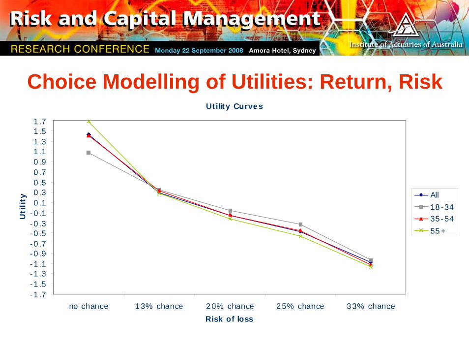
Choice Modelling of Utilities: Return, RiskUtility Curves

-1.7-1.5-1.3-1.1-0.9-0.7-0.5-0.3-0.10.10.30.50.70.91.11.31.51.7

no chance 13% chance 20% chance 25% chance 33% chance

Risk of loss

Uti

lity All

18-3435-54

55+

Choice Modelling of Utilities: Time HorizonUtility Curves

-1.7-1.5-1.3-1.1-0.9-0.7-0.5-0.3-0.10.10.30.50.70.91.11.31.51.7

1 year 3 year 5 year 10 year

Time Horizon

Uti

lity

All18-34

35-5455+

PORTFOLIO INDIFFERENCE CURVES –ISOUTILITIES

pU of f(σ) 1.425 0.295 -0.153 -0.479 -1.087

pU of E(r) 0 13% 20% 25% 33%

-1.352 3.9% 0.07 -1.06 -1.51 -1.83 -2.44

0.121 6.0% - 6.3% 1.55 0.42 -0.03 -0.36 -0.97

0.083 6.5% - 7.2% 1.51 0.38 -0.07 -0.40 -1.00

0.375 7.3% - 8.0% 1.80 0.67 0.22 -0.10 -0.71

0.774 8.0% - 9.0% 2.20 1.07 0.62 0.29 -0.31

E(U) = 2.6296 ln(E(r)) + 3.2612 f(σ) 2 ‐ 8.5644 f(σ) + 8.6409

pU of f(σ) 1.425 0.295 -0.153 -0.479 -1.087

pU of E(r) 0 13% 20% 25% 33%

-1.352 3.9% 0.11 -0.95 -1.47 -1.83 -2.36

0.121 6.0% - 6.3% 1.31 0.25 -0.27 -0.63 -1.16

0.083 6.5% - 7.2% 1.59 0.53 0.01 -0.35 -0.88

0.375 7.3% - 8.0% 1.88 0.82 0.30 -0.06 -0.59

0.774 8.0% - 9.0% 2.16 1.10 0.58 0.22 -0.31

Arithmetic

Function

no chance13% chance

20% chance25% chance

33% chance

3.9%

6.0 - 6.3%

6.5 - 7.2%

7.2 - 8.1%

8.0 - 9.0%

-2.50

-2.00

-1.50

-1.00

-0.50

0.00

0.50

1.00

1.50

2.00

2.50

2.00-2.501.50-2.001.00-1.500.50-1.000.00-0.50-0.50-0.00-1.00--0.50-1.50--1.00-2.00--1.50-2.50--2.00

no chance 13% chance 20% chance 25% chance 33% chance

2.00-3.00

1.00-2.00

0.00-1.00

-1.00-0.00

-2.00--1.00

-3.00--2.00

3.9%

6.5% - 7.2%

6.0% - 6.3%

7.2% - 8.1%

8.0% - 9.0%

Implications

• Monotonic pU’s for E(r) and f(σ) that hold for MRRT.

• Portfolios not necessarily Efficient• Mechanism to drive market equilibrium

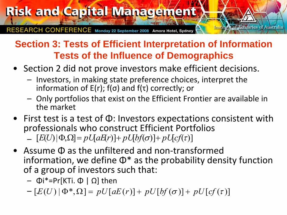
Section 3: Tests of Efficient Interpretation of Information Tests of the Influence of Demographics

• Section 2 did not prove investors make efficient decisions. – Investors, in making state preference choices, interpret the

information of E(r); f(σ) and f(τ) correctly; or– Only portfolios that exist on the Efficient Frontier are available in

the market• First test is a test of Φ: Investors expectations consistent with

professionals who construct Efficient Portfolios – .

• Assume Φ as the unfiltered and non‐transformed information, we define Φ* as the probability density function of a group of investors such that:– Φi*=Pr[KTi. Φ | Ω] then– .

)]([)]([)]([],|)([ τσ cfpUbfpUraEpUUE ++=ΩΦ

)]([)]([)]([]*,|)([ τσ cfpUbfpUraEpUUE ++=ΩΦ

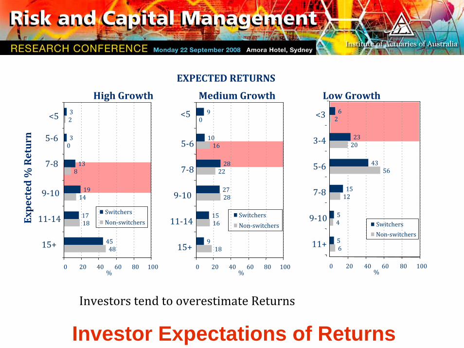
Investor Expectations of Returns

High Growth

EXPECTED RETURNS

Medium Growth Low Growth

Expected % Return

Investors tend to overestimate Returns

3

3

13

19

17

45

2

0

8

14

18

48

0 20 40 60 80 100

<5

5‐6

7‐8

9‐10

11‐14

15+

%

SwitchersNon‐switchers

6

23

43

15

5

5

2

20

56

12

4

6

0 20 40 60 80 100

<3

3‐4

5‐6

7‐8

9‐10

11+

%

SwitchersNon‐switchers

9

10

28

27

15

9

0

16

22

28

16

18

0 20 40 60 80 100

<5

5‐6

7‐8

9‐10

11‐14

15+

%

SwitchersNon‐switchers

Investor Expectations of Risk

7

11

28

28

12

8

5

8

12

26

30

8

10

6

0 20 40 60 80 100

0

1

2

3

4

5

6+

%

Switchers

Non-switchers

Base: All members (n=236)

High Growth

NUMBER OF NEGATIVE RETURN YEARS OUT OF 10 YEARSMedium Growth Low Growth

11

30

33

14

3

2

6

14

16

30

16

6

12

6

0 20 40 60 80 100

0

1

2

3

4

5

6+

%

Switchers

Non-switchers

56

23

5

6

1

4

6

48

18

6

4

6

10

8

0 20 40 60 80 100

0

1

2

3

4

5

6+

%

Switchers

Non-switchers

Years of Negative Return

Investor Expectations of Time Horizon

31

57

8

3

2

30

48

16

6

0

0 20 40 60 80 100

<5

5-10

11-20

21+

DK

%

Switchers

Non-switchers

Base: All members (n=236)

High GrowthYEARS UNTIL MATURATION OF INVESTMENT

Medium Growth Low Growth

42

49

4

3

2

26

54

12

8

0

0 20 40 60 80 100

<5

5-10

11-20

21+

DK

%

Switchers

Non-switchers

60

25

8

5

2

48

30

8

14

0

0 20 40 60 80 100

<5

5-10

11-20

21+

DK

%

Switchers

Non-switchers

Expected years until m

aturation

Personality and Demographics may matter

Education Levels Switchers%

Non-Switchers%

Some secondary school 4 8

Intermediate/School Certificate 11 16

Leaving Certificate/HSC 14 18

Trade qualification/Diploma 35 40

University Undergraduate Degree 19 12

ISTJ ISFJ INFJ INTJ

ISTP ISFP INFP INTP

ESTP ESFP ENFP ENTP

ESTJ ESFJ ENFJ ENTJ

ISTJ ISFJ INFJ INTJ

ISTP ISFP INFP INTP

ESTP ESFP ENFP ENTP

ESTJ ESFJ ENFJ ENTJ

S S N N

I 18% 4% 12% 4% J

I 8% 4% 2% 2% P

E 10% 2% 2% 4% P

E 16% 2% 4% 6% J

T F F T

S S N N

I 13% 3% 3% 6% J

I 7% 3% 2% 2% P

E 11% 3% 1% 3% P

E 19% 5% 4% 16% J

T F F T

SWITCHERS NON-SWITCHERS

Conclusion

• Expectations showed a dispersion Pr(Φ*)• Ω, the conditioning of E(U) based on

demographics or other investor characteristics, debatable whether in aggregate, this characterizes the effects of the transform of Φ.

• . )]([)]([)]([*]]Pr[|)([ τσ cfpUbfpUraEpUUE ++=Φ

Section 4: Event Studies• .• For trade:• But require information change:

– .– New orthogonal constraint B

• Is an event proof of change of information or some other constraint?

• Inertia– Bernoulli variable X, where – E(X) = 1[E(U*)‐E(U)]>θ for trade to occur– Threshold θ that is set endogenously by each investor:

)]([)]([)]([*]]Pr[|)([ τσ cfpUbfpUraEpUUE ++=Φ)()( *

ii UEUE >

Φ∂∂

∂∂

=Φ∂

∂=−

),),((.),),((

)()()()( 11*

1τσ

τσrE

rEUEUE

UEUE i

),....,(),...,(),...,)(( 212121 nnni qqqBqqqTqqqUEL μλ −−=

Dispersion of Pr[Φ] and Event study explain why only some choose

θ )]([)]([)]([*]]Pr[|)([ τσ cfpUbfpUraEpUUE ++=Φ

E(X) = 1[E(U*)-E(U)]>θ

Event StudyCorrelation of Age with Risk Shift

R2 = 0.7164

-5

-4

-3

-2

-1

0

1

40 45 50 55 60 65

Median Age of Segment

Ris

k Sh

ift

Age versus Risk Prof ileLinear (Age versus Risk Shift)

Pre 1 October 2005

Post 1 October 2005

‘Risk Values’

High Growth +1

Trustee Selection Trustee Selection 0

Diversified ‐1

Balanced ‐2

Cap Guarded ‐3

Cash ‐4

Information received by investors consistently interpreted ; choices made were entirely reliant on removal of constraint (B).

holds),....,(),...,(),...,)(( 212121 nnni qqqBqqqTqqqUEL μλ −−=

Section 5: Continuous time analysis

• Consistent Method of assigning values to ‘Riskiness’ for quantitative analysis

Portfolio Names‘High

Growth’‘Trustee

Selection’‘Divers-

ified’ ‘Bal-anced’ ‘Capital Guarded’ ‘Cash’

Typical Assets held85-90% Equities, Property

75% - 85% Equities, Property

65-70% Equities, Property

45-55% Equities,

Property, with the remainder

in Bonds, Cash

<15% Equities,

Property, with the remainder

in Bonds, Cash

Largely Cash with possibly some short-dated Bonds

Relative Risk ‘Value’ +1 0 -1 -2 -3 -4

Risk Shifts and Market Direction

Risk Shifts by Superannuation Investors

1.0

1.5

2.0

2.5

3.0

3.5

4.0

1/07

/200

2

1/09

/200

2

1/11

/200

2

1/01

/200

3

1/03

/200

3

1/05

/200

3

1/07

/200

3

1/09

/200

3

1/11

/200

3

1/01

/200

4

1/03

/200

4

1/05

/200

4

1/07

/200

4

1/09

/200

4

1/11

/200

4

1/01

/200

5

1/03

/200

5

1/05

/200

5

1/07

/200

5

1/09

/200

5

1/11

/200

5

1/01

/200

6

1/03

/200

6

Uni

t Pric

e Se

ries

of A

ustr

alia

n Eq

uitie

s

-6

-4

-2

0

2

4

6

Ris

k M

ovem

ents

Indexed Equities PerfRisk BiasLog. (Indexed Equities Perf)30 per. Mov. Avg. (Risk Bias)Linear (Risk Bias)

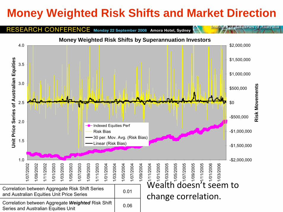
Money Weighted Risk Shifts and Market Direction

Wealth doesn’t seem to change correlation.

Correlation between Aggregate Risk Shift Series and Australian Equities Unit Price Series 0.01

Correlation between Aggregate Weighted Risk Shift Series and Australian Equities Unit 0.06

Money Weighted Risk Shifts by Superannuation Investors

1.0

1.5

2.0

2.5

3.0

3.5

4.0

1/07

/200

2

1/09

/200

2

1/11

/200

2

1/01

/200

3

1/03

/200

3

1/05

/200

3

1/07

/200

3

1/09

/200

3

1/11

/200

3

1/01

/200

4

1/03

/200

4

1/05

/200

4

1/07

/200

4

1/09

/200

4

1/11

/200

4

1/01

/200

5

1/03

/200

5

1/05

/200

5

1/07

/200

5

1/09

/200

5

1/11

/200

5

1/01

/200

6

1/03

/200

6

Uni

t Pric

e Se

ries

of A

ustr

alia

n Eq

uitie

s

-$2,000,000

-$1,500,000

-$1,000,000

-$500,000

$0

$500,000

$1,000,000

$1,500,000

$2,000,000

Ris

k M

ovem

ents

Indexed Equities PerfRisk Bias30 per. Mov. Avg. (Risk Bias)Linear (Risk Bias)

Conclusion : Generalised Utility• Firstly, the utility function of the aggregation of investors can be

written in the form:

•– Where: Φi*=Pr[KTi. Φ | Ω]

– Investors optimise to MRRT (Market Risk / Reward Theorem), don’t necessarily choose efficient portfolios.

• Secondly, no evidence that demographic factors are conditions on aggregate utility.

• Thirdly, event studies show that trade occurs for reasons other than changes in information– .

• E(X) = 1[E(U*)‐E(U)]>θ presents inertia

)]([)]([)]([*]]Pr[|)([ τσ cfpUbfpUraEpUUE ++=Φ

),....,(),...,(),...,)(( 212121 nnni qqqBqqqTqqqUEL μλ −−=