empirical research regarding discounts for lack of ... · business valuation update, vol. 19, no....
TRANSCRIPT

EMPIRICAL RESEARCH REGARDING
DISCOUNTS FOR LACK OF MARKETABILITY
Volume 1.1 – July 2019
______________
Marc Vianello, CPA, ABV, CFF Managing Member, Vianello Forensic Consulting, LLC
With data analysis assistance by Aleksandrs Sverdlovs

Copyright © 2007-2019 Vianello Forensic Consulting, LLC
1
Introduction by Francis A. Longstaff, Ph.D.
The question of how to value illiquid investments that cannot be traded continuously is one of the most challenging issues facing academic researchers and industry practitioners. The reason for this is that the lack of marketability takes us well outside standard paradigms in financial economics such as the notion of efficient markets, portfolio choice, and the usual risk and return tradeoffs that underlie much of modern investment theory. Marc Vianello's book “Empirical Research Regarding Discounts for Lack of Marketability'' is an impressive effort to bring a rigorous and comprehensive data-based perspective to addressing these issues. The book begins with a thorough review of the historical research on the topic and provides valuable insights about the scope and reliability of the evidence. The book then moves on to an insightful analysis of the strengths and weaknesses of existing models of the discount for lack of marketability. What makes this analysis particularly valuable is the depth of knowledge and practical experience the author brings to the task. Finally, the book offers a number of carefully considered extensions to existing models, demonstrates how these can be implemented in practice, and evaluates their performance using objective empirical standards. This book makes great strides in helping us understand the nature of the discount for lack of marketability phenomenon and offers us valuable perspectives on how to address the associated challenges of valuation. Francis A. Longstaff, Ph.D. Allstate Chair in Insurance and Finance Anderson School of Management University of California at Los Angeles

Copyright © 2007-2019 Vianello Forensic Consulting, LLC
2
Introduction by Michael Gregory, ASA, CVA, MBA
With a dedication to improve analytics for business valuers, Marc Vianello has diligently and passionately conducted his research on Discount for Lack of Marketability over many years. As a result of his research he has shed light on the shortcomings of many existing models, and he has developed a tool that is based on real world data and that has been accepted by the courts. After a careful look at the literature followed by a critique of major sources commonly used by business valuers, the author presents very significant findings. An analysis of the data with graphs, charts and statistical measures presents reasons to question currently accepted approaches. Starting with Longstaff model probability is incorporated into a new model considering the mean and standard deviation of market timing and volatility. The author presents how to obtain these measures from existing data sources (systemic) and provides the business valuer with insights with how to consider the application of non-systemic professional judgment. From the text the author states, “Double probability DLOMs calculated using the Longstaff formula provided values most consistent with the empirical evidence provided by the discounts of corresponding restricted stock transactions. The calculated DLOMs should be considered systematic. The currently available empirical information supports the conclusion that double probability DLOMs calculated using the VFC Longstaff methodology results in reliable estimates of systematic DLOM.” This is very significant in that no other source can make such a claim. This is a tool that no business valuer should be without. Michael Gregory, ASA, CVA, MBA Former IRS Engineering Territory Manager Champion of the IRS DLOM Job Aid

Copyright © 2007-2019 Vianello Forensic Consulting, LLC
3
About the Author
Marc Vianello, CPA, is the owner of Vianello Forensic Consulting, LLC. He is accredited in the business valuation (ABV) and certified in financial forensics (CFF by the American Institute of Certified Public Accountants. Mr. Vianello graduated in 1975 from the University of Missouri, cum laude, with a Bachelor’s Degree in Business Administration and a major in Accountancy. A former financial statement auditor, tax consultant, public utility rate consultant, and entrepreneur, Mr. Vianello has spent most of his professional career providing expert testimony in highly complex commercial litigation.
Previously Published Content Some of the content in this book reflect Mr. Vianello’s previously published articles listed below. The concepts underlying the articles have been corroborated by the research presented in this book. Previously presented thoughts regarding adjustments to the Longstaff formula are superseded by this book. "New Insight into Calculating Discounts for Lack of Marketability," Financial Valuation and Litigation Expert, Issue 11, February/March 2008; republished by CPA Expert, May 2008.
"Restructuring the Levels of Value," BVR's Guide to Discounts for Lack of Marketability, 2009 Edition.
"Calculating DLOM Using the VFC Longstaff Methodology," BVR's Guide to Discounts for Lack of Marketability, 2009 Edition. "The Specific Company Risk of Abnormal Levels of Debt," Valuation Strategies, September/October 2010 Edition.
"The Marketing Period of Private Sales Transactions," Business Valuation Update, Vol. 16, No. 12, December 2010
"The Marketing Period of Private Sale Transactions: Updated for Sales through 2010," Business Valuation Update, Vol. 17, No. 11, November 2011.
"Rebutting Critics of the Longstaff DLOM Methodology," Business Valuation Update, Vol. 18, No. 9, September 2012.
"Why Do Private Firms Linger on the Selling Block?" Business Valuation Update, Vol. 19, No. 10, October 2013.
"How Probability Affects Discounts for Lack of Marketability," Business Valuation Update, Vol. 20, No. 7, July 2014.
"Using Restricted Stock and Pre-IPO Studies for Quantifying DLOM - Two Ways of Saying I Don't Know?” Valuation Strategies, September/October 2014 Edition. "Calculating Probability Based DLOMs," Valuation Strategies, November/December 2014 Edition. "Probability Based Estimation and the DLOM Calculation," QuickRead, August 19, 2015 (a National Association of Certified Valuators and Analysts publication).

TABLE OF CONTENTS
Introduction by Francis A. Longstaff, Ph.D. Page 1 Introduction by Michael Gregory, ASA, CVA, MBA Page 2 About the Author Page 3 Previously Published Content Page 3 Preface Page 6 Chapter 1 Replacing the Traditional View of Levels of Value Page 8 Chapter 2 The Interrelationship of Empirical Studies of Discounts and Liquidity Page 14
Chapter 3 The Empirical Studies of Restricted Stocks and Initial Public Offerings Are Inadequate for Estimating DLOM Page 18
Section 1 Restricted Stock Studies Page 19 Section 2 Pre-IPO Studies Page 23 Chapter 4 The Pluris
® Restricted Stock Database Page 27
Section 1 What is the Pluris
® DLOM Database? Page 27
Section 2 Are the Pluris Transactions “Accurate”? Page 28 Section 3 Some Identified Problems with the Pluris® DLOM Calculator Page 29 Section 4 Pluris
® Discount / Premium Measurement Page 30
Section 5
Discount Correlation with Total Assets, Market Value-to-Book Value Ratio, 12-Month Stock Price Volatility, Percentage of Shared Outstanding, and Calendar Quarters to Sell Page 32
Section 6
The Discounts Reported in the Pluris® DLOM Database Are Not
Consistent with Past Changes in SEC Rule 144 Required Holding Periods Page 43
Section 7 Correlation of the Pluris
® Restricted Stock Discounts and Valuation
Metrics Page 44 Section 8 Using the Pluris
® Database for Benchmarking Page 49
Section 9 Using the Pluris
® Methodology for Calculating DLOM Page 55
Chapter 5 The Stout Restricted Stock Study Page 67 Section 1 Exploring the Stout Restricted Stock Study Page 67
Section 2 The Association of Certain Company Statistics and Restricted Stock Discounts Page 76
Section 3
The Discounts Reported in the Stout Restricted Stock Study Are Consistent with Past Changes in SEC Rule 144 Required Holding Periods Page 87

Copyright © 2007-2019 Vianello Forensic Consulting, LLC
5
Section 4 How the Stout Restricted Stock Study Discounts Correlate with the Other Metrics Reported in the Database Page 87
Section 5 The Stout DLOM Methodology Page 91 Section 6 Testing the Stout DLOM Methodology Page 94 Chapter 6 The Price and Time Variables that Underlie DLOM Page 98 Section 1 Marketing Periods or Privately Held Businesses Page 99 Section 2 The Registration Periods of Public Offerings Page 106 Section 3 Price Volatility Page 114 Section 4 Enhanced Probability Estimation Page 121
Section 5 The DLOM Effects of Restricted Stock versus Private Company Illiquidity Periods Page 123
Chapter 7 Longstaff Formula DLOMs and the IRS Page 125 Section 1 The “Perfect Timing” Criticism Page 131 Section 2 The “Formula Breaks Down” Criticism Page 131 Section 3 The Effects of Standard Deviation on Probability Distributions Page 133 Section 4 Adding Probability to the Longstaff Formula Page 134 Section 5 Single Probability DLOM Page 137 Section 6 Double Probability DLOM Page 141 Chapter 8 Price Volatility and Discounts for Lack of Marketability Page 148 Section 1 The Reliability of Stock Price Data for Price Volatility Estimation Page 148
Section 2 The Relationship of DLOMs Based on the Longstaff and Black-Scholes Formulae Page 154
Section 3 The Relationship of Probability-Based Option DLOMs to Restricted Stock Discounts Page 156
Chapter 9 A VFC Double Probability DLOM Case Study Page 165 Chapter 10 Revisiting “Litman Audacity” Page 175 Chapter 11 Conclusions Page 178 Appendix Guide for Using the VFC DLOM Calculator
® Page 179

Copyright © 2007-2019 Vianello Forensic Consulting, LLC
6
PREFACE
The appropriate amount of discount for lack of marketability (“DLOM”) has long been
critical for valuation professionals, investors in and issuers of illiquid securities, financial
statement issuers and auditors, the courts, and others. The determination of an appropriate
discount has been extensively discussed and debated. Yet, to this author’s knowledge, no one
has heretofore made the intensive empirical study necessary to actually justify a DLOM
methodology using stringently-defined, objective data. That is the purpose of this research.
The research presented herein has been years in development. The analyzed data
provides extensive insight into the market evidence of liquidity discounts. And the data supports
and challenges different methodologies for determining DLOMs. The study results strongly favor
basing DLOM estimation on probability-based option modeling as opposed to other commonly
available means.
The data used in this research is necessarily limited to that available at the time the
analysis was done. It uses extensive transactional data possessed, or otherwise accessible, by
the author. Much of it should be updated as new data becomes available. In particular,
transactions that have been added to the Pluris®, Stout (formerly FMV Opinions
®), BIZCOMPS
®,
and DealStats® (formerly Pratt’s Stats) databases. Those additions are a matter for a future
supplement of this research. The author invites those issuers to participate in his research
efforts.
Two other limitations affected our research. First, our analyses were hampered by a lack
of restricted stock issuer daily price data more than 10 or 20 years old depending on the price
data source. Daily price data is necessary to determine price probability volatilities. 1,687
restricted stock transactions escaped analysis because daily price history before the transaction
dates was not available to the author. More price data may be available from other sources not
currently available to the author. The Center for Research in Security Prices (“CRSP”) is one
potential source. Second, much of the restricted stock transactional discount data available
through Pluris® is tainted with warrants. 1,867 transactions escaped analysis because of the
manner in which Pluris® values warrants and, therefore, restricted stock discounts. Repricing the

Copyright © 2007-2019 Vianello Forensic Consulting, LLC
7
warrants using the Black-Scholes formula might yield analytically viable data, which the author
invites Pluris® to do, and to provide.
The author invites qualified interested parties to participate in his continuing DLOM
research.
Finally, the author extends his gratitude to the Business Valuation Committee of the
American Institute of Certified Public Accountants for its assistance, recommendations, and
encouragement in completing this book.
Marc Vianello, CPA, ABV, CFF
July 1, 2019

Copyright © 2007-2019 Vianello Forensic Consulting, LLC
8
Chapter 1
LIQUIDITY AND LEVELS OF VALUE
Liquidity represents the ability to sell an investment quickly when the investor decides to
sell. Conversely, lack of liquidity, although having many causes,1 has the cost of failing to realize
gains or failing to avoid losses on an investment during the period in which the investor is offering
it for sale. With that understanding, discounts for lack of marketability ("DLOM") should reflect the
illiquidity cost of the investment—its value volatility—during the period of time that it is being
marketed for sale.
The valuation profession has written volumes about “levels of value” over the years.
One concept has placed a higher value on “control” than on “liquidity.” The relative levels of
value under this “Control Dominant” structure are presented as –
Control Value
Difference reflects the value of control
Publicly Traded Value
Difference reflects the value of marketability
Non-Marketable Minority Value
Under the Control Dominant concept, the “control premium” regularly measured by
MergerStat® has been offered as proof that Control Value is worth more than Publicly Traded
Value, assuming that all other things are equal. But does the Control Dominant concept hold if
the interpretation given to MergerStat’s® “control premium” is incorrect, and that it instead
measures the discount (or a portion of the discount) imposed by non-strategic investors on poorly
run public companies? Another example of potentially faulty Control Dominant logic is the notion
that Publicly Traded Value exclusively represents the return expectations of minority
stakeholders. But does the Control Dominant view hold if instead the returns realized on publicly-
traded securities represent risk adjusted rates at which the expectations of all marginal non-
strategic investors are equalized based on the expected cash flows of the enterprise? Others
hold the view that Control Value equates to Publicly Traded Value, giving “control” a presumption
of virtually immediate liquidity. But does this alternative hold considering the time periods
necessary to sell a controlling interest and associated transaction costs?
When comparing the relative values of controlling and minority interests in the same
privately-held company, it is easy to intuit that the ability to control the enterprise is worth more
1 A non-exhaustive list of causes of illiquidity includes lack of buyers, excessive pricing,
transaction costs, business complexity, income stream risk, and much more.

Copyright © 2007-2019 Vianello Forensic Consulting, LLC
9
than not having that ability. Hence, all other things equal, Control Value is logically greater than
Minority Value. But that logic does not lead to a conclusion that Control Value is greater than
Publicly Traded Value on a per share basis. Imagine a controlling interest in a publicly traded
company. The controlling investor owning a comparatively large or unregistered block of stock is
exposed to the same price volatility as the minority investors, but is denied the opportunity to as
quickly dispose of his interest in the company. This realization suggests that liquidity (because it
offers the ability to protect the value of one’s investment) is worth more than control share-for-
share.
Let us explore the factors that result in different levels of value. When comparing the
value drivers of well run publicly traded businesses (value based on non-controlling stock trades)
and well run privately controlled businesses (value based on the entirety), we find that the only
real difference is liquidity or its lack:
Public Companies
Earnings / Cash Flow Growth potential Industry Risk Size Risk Market Fluctuations Liquidity
Private Companies
Earnings / Cash Flow Growth potential Industry Risk Size Risk Market Fluctuations No Liquidity
With the understanding that liquidity represents the ability to sell an investment quickly
without price impact and little transaction cost when the investor decides to sell in order to lock in
gains or to avoid losses, then, assuming everything else to be equal, the inability to quickly
liquidate a controlling interest in a publicly traded company suggests that it is worth less per share
than the liquid minority shares. That observation leads initially to this Restructured View of the
levels of business value:
Publicly Traded Value
Difference reflects the economic risk of lack of marketability
Illiquid Control Value
Difference reflects the economic risk of lack of control
Non-Marketable Minority Value
The basis of this Restructured View is straightforward. First, the investment returns of
publicly traded companies should be viewed as “public company returns” not as “marketable
minority returns.” For well run companies that are operating optimally for their shareholders,
there should be no economic difference (aside from compliance costs) between public company
operating results and those accruing to controlling interests of otherwise identical private

Copyright © 2007-2019 Vianello Forensic Consulting, LLC 10
companies – the material perquisites of control have been squeezed out of the public companies.
Poorly run companies (i.e. those not operating optimally for their shareholders) have difficulty
maintaining shareholder value and raising new capital.2 Consequently, publicly traded
companies that are not optimized have difficulty attracting capital in the form of fractional
ownership.
Second, Strategic Value does not enter into the determination of required rates of return,
which are based on the prices of shares actually traded. Although an increase in stock price may
be offered to existing shareholders as an inducement to sell, the actual benefits of a strategic
acquisition accrue to the merged company as revenues are enhanced and expenses are
minimized. Such effects are reflected in the income statement and cash flow of the enterprise as
a whole and contribute to increased value that is shared by all post-acquisition ownership
interests. Such effects are not suggestive of the notion that Strategic Value is worth more than
Publicly Traded Value. Although a value may be derived from a strategic opportunity, it does not
mean that the opportunity is worth more than the value of liquidity once the opportunity is
realized. After all, once the opportunity is realized, the merged-company owners are subject to
return volatility just as the owners of publicly traded securities are. This price risk applies to all
owners of the enterprise, whether they hold registered or unregistered shares, restricted or
unrestricted shares, and controlling or minority shares.
There are well run publicly traded companies and well run privately held companies.
There are also poorly run companies of both types. When a public company is acquired at a
premium above its publicly traded value it is a reflection of the perception that the acquired
company is not maximizing its economic opportunities and shareholder value. Well-run publicly
traded companies (i.e. those that are maximizing their economic opportunities and shareholder
value) are not taken private—they are too expensive. This is not to say that an acquirer cannot
simply overpay or that two well-run public companies cannot merge to take advantage of market
opportunities that have nothing to do with management deficiencies. Obviously, such
acquisitions happen. But these scenarios nonetheless reflect expectations of post-acquisition
benefits not being realized by the acquired company. Accordingly, the “premium” observed when
publicly traded companies are taken private reflects the anticipation that some nature of
inefficiencies in the acquired company can and will be eliminated. For these reasons, the so-
called “control premium studies” are misused when used to suggest that control is worth more
than liquidity.
2 Some have observed that cash flows underlying Publicly Traded Value minus the benefits of
liquidity equate to those underlying Illiquid Control Value minus the benefits of control. While conceptually legitimate, there is no known empirical means of equating the benefits of liquidity and the benefits of control, and the two benefits may be far from equal. This negates the usefulness of the observation.

Copyright © 2007-2019 Vianello Forensic Consulting, LLC 11
Consider these thoughts: (1) Risk adjusted rates of return are fungible.3 (2) There is a
transaction cost to becoming and continuing as a publicly traded company. This creates a
disincentive that can only be justified by (a) greater access to capital, and (b) the “pop” in value
that the pre-IPO owners receive when their business goes public. (3) If control were worth more
than liquidity, then the owners of privately held businesses would have a further disincentive to
going public. (4) If control were more valuable than liquidity, then there would be no public
companies.4 (5) If control were worth more than liquidity, then large private equity firms such as
Blackstone and KKR would never convert to publicly traded companies. It seems counter-
intuitive that control should be viewed as equal in value to—or even more valuable than—
liquidity.
Under otherwise identical circumstances, any given investment should have a greater
value if it is immediately marketable than if it is not. Why is this so? Because liquidity allows the
investor to avoid the economic risks of illiquidity.
The notion of a control premium vis-à-vis public company values is economically illogical.
Such premiums mathematically equate to lower rates of return. But since it is expected that it
would take longer to sell a controlling interest in an optimally run private company than the
comparable interest in an otherwise identical public company, the required rate of return of the
private company investor should be greater, not lower, than that of the public company investor.
Thus, private company values should reflect a discount, not a premium, relative to comparable
public company values.
Figure 1.1 presents the Restructured View of value in greater dimension. The depiction
shows how well run and poorly run private companies relate to each other and how the
opportunity to realize strategic value (including market synergies) arises from the conversion of
poorly run firms into firms that hopefully will be well run. The depiction also demonstrates that all
privately held companies—even controlling interests—are subject to the cost of illiquidity.5 Even
3 Eric W. Nath, ASA, and M. Mark Lee, CFA “Acquisition Premium High Jinks,” 2003 International
Appraisal Conference, American Society of Appraisers; Eric W. Nath, ASA, “How Public Guideline Companies Represent ’Control’ Value for a Private Company,” Business Valuation Review, Vol. 16, No. 4, December 1997; and Eric W. Nath, “Control Premiums and Minority Discounts in Private Companies,” Business Valuation Review, Vol. 9, No. 2, June 1990. 4 Id.
5 It has been suggested by some practitioners that discounts for lack of liquidity should not be
applied to controlling interests because the earnings and cash flow of the company offset the discount while it is being held for sale. This argument fails because (1) it relies on a flawed view of the levels of value that ignores that (a) rates of return derive from analysis of publicly traded stocks, and (b) liquidity is the only driver of value of publicly traded companies not present in otherwise identical privately held companies; (2) the economic circumstance of holding period earnings and cash flow also exists for minority interests; and (3) the holding period earnings and cash flow of both controlling interest and minority interest investments are necessarily already included in the capitalized or discounted values of the investments.

Copyright © 2007-2019 Vianello Forensic Consulting, LLC 12
assuming all other things being equal, it simply takes longer to sell a controlling interest in a
privately held business than it takes to sell an interest in a comparable publicly traded company.
Minority interests in privately held companies are worth proportionately less than controlling
interests for two reasons: (1) such minorities generally lack the ability of controlling owners to
realize the perquisites of ownership, and (2) the economic risks of lack of control result in longer
periods of time to sell minority interests than it takes to sell the controlling interest in the same
private company.
Well Run
Well RunWell Run
Well Run
MGMT
MGMTMGMT
MGMT
QUALITY
QUALITYQUALITY
QUALITY
Poorly Run
Poorly RunPoorly Run
Poorly Run
DLOM
DLOMDLOM
DLOM
DLOM
DLOMDLOM
DLOM
Well Run
Well RunWell Run
Well Run
MGMT
MGMTMGMT
MGMT
QUALITY
QUALITYQUALITY
QUALITY
Poorly Run
Poorly RunPoorly Run
Poorly Run
NO
NO NO
NO
CONTROL
CONTROLCONTROL
CONTROL
NO
NO NO
NO
CONTROL
CONTROLCONTROL
CONTROL
Well Run
Well RunWell Run
Well Run
MGMT
MGMTMGMT
MGMT
QUALITY
QUALITYQUALITY
QUALITY
Poorly Run
Poorly RunPoorly Run
Poorly Run
Strategic
Strategic Strategic
Strategic
Value
ValueValue
Value
Opportunities
OpportunitiesOpportunities
Opportunities

Copyright © 2007-2019 Vianello Forensic Consulting, LLC 13
Whether a private company can be sold via public offering is a critical valuation
consideration. Chapter 6 [to be renumbered] discusses the empirical evidence of the time
required to sell private company and to obtain SEC approval for a public equity offering. Table
1.1 summarizes the average marketing times by broad Standard Industrial Classification.
Equating S-1 filing with a private company brokerage listing, Table 1.1 shows that it typically
takes more than twice the time to complete a private company sale than to obtain approval for a
public offering. The shorter marketing periods for companies for which a public offering is a
viable alternative should result in lower discounts for lack of marketability if all other things are
equal. Of course, many things necessary for a public filing may be completed in advance, and
many things necessary for a private sale may occur after brokerage listing. And some large
companies may be able to be sold privately within a public offering time frame. Such
circumstances would narrow the valuation differences between the two marketing paths.
Nevertheless, there must be a value increment that incentivizes public registration or there would
be no publicly traded companies.
Table 1.1
Average Number of Days to Complete a Sale or Offering
16,499 Private Company Sales
5,157 Approved Public Offerings
Private Sale to Public Offering
Time Factor SIC Code
Range
0000-0999 216 123 1.8
1000-1999 271 103 2.6
2000-2999 235 95 2.5
3000-3999 238 97 2.5
4000-4999 217 100 2.2
5000-5999 210 93 2.3
6000-6999 206 103 2.0
7000-7999 211 93 2.3
8000-8999 212 96 2.2
9000-9999 63 0 n/a
All industries 211 97 2.2

Copyright © 2007-2019 Vianello Forensic Consulting, LLC 14
Chapter 2
THE INTERRELATIONSHIP OF EMPIRICAL STUDIES OF DISCOUNTS AND LIQUIDITY
Conventional business valuation has used the well-publicized results of restricted stock
studies, pre-IPO studies, and registered versus unregistered stock studies to effectively guess at
appropriate DLOM percentages to use in their valuation reports. Understandably, such subjective
means of applying the traditional approaches have been broadly unsatisfactory to the valuation
community and the courts.
Figure 2.1
The Interrelationship of Observed Risk, Liquidity, and Discounts
INCREASING MARKETING TIME
>>>>>>>>>>>>>>>>>>>>>>>>>>>>>>>>>>>>>>>>>>>>>>>>>>>>>>>>>>>>>>>>>
NEAR-IMMEDIATE LIQUIDITY
MODERATE LIQUIDITY ILLIQUID VERY ILLIQUID
INC
RE
AS
ING
RIS
K A
ND
DIS
CO
UN
TS
AS
MA
RK
ET
ING
PE
RIO
DS
INC
RE
AS
E
>>
>>
>>
>>
>>
>>
>>
>>
>>
>>
>>
>>
>>
>>
>>
>>
>>
>>
>>
>>
>>
>>
>>
>>
Publicly Traded Stocks
Private Sales of
Registered Stocks
Private Sales of Restricted Stocks with Registration
Rights
Private Sales of
Unregistered Stocks
Pre-IPO Control Value
Private Company Control Value
Pre-IPO Minority Value
Private Company Minority Value

Copyright © 2007-2019 Vianello Forensic Consulting, LLC 15
Figure 2.1 presents a stratification of the types of empirical studies that researchers have
performed to explore the cost of illiquidity. The study types are shown in theoretical relative
position based on marketing time and volatility assuming all other aspects of investment as equal.
Although Figure 2.1 shows a stair-stepping of the studies, it is not the intent of the presentation to
suggest that linear reduction of value results.6 The presentation is, instead, intended to enhance
understanding of what the various studies are measuring, how they interrelate, and the extent to
which they meet the needs of business valuation discount analysis.
• Publicly traded companies are the standard against which all of the studies measure
results and from which rates of return are calculated. Interests in publicly traded
companies are worth more than interests in identical privately held companies
because they can be sold immediately to realize gains and to avoid losses, while
interests in privately held companies cannot. Although there are costs to being a
publicly traded company, the assumption is that such costs are more than offset by a
lower cost of capital. If this were not inherently true then there would be no economic
justification for incurring those costs.
• Private sales of publicly registered stocks typically involve large blocks of stock that
could be sold into the public marketplace, but which would materially adversely affect
stock prices if the entire block were to be dumped into the market at once. Avoiding
that price effect results in an extended period of time to liquidate the investment
position in the public market during which time the investor is subject to market risk.
Negotiating a private sale of the block can accelerate liquidating the position, but
requires a buyer with the wherewithal to purchase the block. Such buyers can
reasonably expect a price discount relative to the publicly traded price. Although
private sales of large blocks of registered stocks may somewhat mitigate the market
risk by potentially shortening selling periods, the risk does not go away. The buyer of
the block assumes the risks, in turn, of having to sell to another qualified buyer or
slowly feeding the block into the public market. These risks require compensation by
means of a discount (i.e. DLOM).
• Private sales of restricted stocks in public companies have the same price risks as
private sales of large blocks of registered stocks, but have the additional risk of being
locked out of the public market for specific periods of time or being subject to
restrictive “dribble out” rules. Accordingly, restricted stocks often can only be sold
quickly in private sale transactions, which take longer than it does to sell unrestricted
6 The relative value of specific companies should be considered in the framework of Figure 1.1,
which provides an understanding of why, for example, public companies are sometimes taken private.

Copyright © 2007-2019 Vianello Forensic Consulting, LLC 16
stocks in the public market.7 The result is that a restricted registered stock is worth
less than an unrestricted stock in the same company because of the greater market
risk associated with the extended marketing period.
• Private sales of unregistered stocks in public companies typically involve large blocks
of stock. They are worth less than equivalent blocks of registered stock (whether
restricted or unrestricted) in the same publicly traded company because there is a
cost for eventual registration that directly lowers value and can dissuade potential
buyers.8 The result is relatively greater uncertainty, relatively longer time to market
the interest, and relatively greater exposure to the risks of the marketplace.
• Pre-IPO private sales of controlling interests should have relatively longer marketing
periods than for private sales of unregistered stocks in public companies, because
the fact and timing of the IPO event can be uncertain. Furthermore, low pre-IPO
stock sales prices may reflect compensation for services rendered. This author is not
aware of any studies that specifically address discounts observed in sales of
controlling interests in pre-IPO companies.
• Private sales of controlling interests in a company that has no expectation of going
public should be worth less than an otherwise identical company with an anticipated
IPO event. The marketing period for a business with an anticipated IPO event should
be shorter than the marketing period of a business that is not anticipating such an
event.
• Pre-IPO sales of non-controlling interests in a company planning an IPO event
should be worth less than the controlling interest in the same company even without
the planned IPO. The inability to control whether the planned IPO goes forward
should result in greater uncertainty and a longer marketing period to liquidate the
investment than would be experienced by the controlling investor. Low pre-IPO
share prices may also reflect compensation for services rendered.
• Non-controlling interests in private companies require greater discounts than all of
the preceding circumstances because the relative risks of lacking control cause the
7 Some restricted stocks cannot be sold at all for contractually determined periods of time. Such
investments have even greater economic risks than those merely subject to the “dribble out” rules. 8 This discount is considered by Mukesh Bajaj, David J. Dennis, Stephen P. Ferris and Atulya
Sarin in their paper “Firm Value and Marketability Discounts.” Their study isolates the value of liquidity by comparing the stock sales of 88 companies that had sold both registered and unregistered stock private offerings. This approach does not, however, address the discount applicable to the additional time it takes to sell controlling or minority interests in private companies. Instead, it measures the value of stock registration. See Section IV.C of “Firm Value and Marketability Discounts.”

Copyright © 2007-2019 Vianello Forensic Consulting, LLC 17
period of time to liquidate the position to be potentially much longer than for the
controlling interest in the same company or for otherwise comparable minority
positions in firms with a planned IPO event.

Copyright © 2007-2019 Vianello Forensic Consulting, LLC 18
Chapter 3
THE EMPIRICAL STUDIES OF RESTRICTED STOCKS AND INITIAL PUBLIC OFFERINGS ARE INADEQUATE FOR ESTIMATING DLOM
Restricted stock and pre-IPO studies have been used to quantify DLOM since the early
1970s. Despite making a good case for the need for a DLOM when valuing an investment that is
not immediately marketable, the study results are unreliable for calculating the DLOM applicable
to a particular valuation engagement for a variety of reasons discussed below.
Although the empirical studies of marketability discounts provide a wealth of empirical
evidence of the discounts that market participants demand on risky assets, the studies have
limited utility to the appraiser opining on the fair market value of a business interest. Several
authors have noted, for example, that most publicly traded firms do not issue restricted stock.
This dearth necessitates study samples of limited sizes, in limited industries, with data spread
over long periods of time. The result has been substantial standard errors in discount estimates.
The restricted stock studies measure the difference in value between a publicly traded
stock with and without a time restriction on sale. Left unanswered is whether there is a difference
between the restricted stock value of a publicly traded company and the value of the same
company if it were not publicly traded at all.
The pre-IPO studies reflect substantial standard errors in their estimates for similar
reasons, but are also distorted by the fact that the studies necessarily are limited to successful
IPOs; there are no post-IPO stock prices for failed IPOs. The discounts observed in the pre-IPO
studies may also reflect uncertainty about whether the IPO event will actually occur,9 when the
IPO event will occur, at what price the event will occur, and whether the pre-IPO price reflects
compensation for any reason.
It should be noted that all of the companies in the restricted stock and pre-IPO studies
are, in fact, publicly traded. But essentially none of the privately held companies that are the
subject of business valuations have a foreseeable expectation of ever going public. Accordingly,
the circumstances of the privately held companies are highly distinguishable from those of the
publicly traded companies that are the subjects of the studies. Thus, the pre-IPO studies are of
dubious value for determining the DLOM of privately held companies.
Bajaj, et al., studied the difference in value observed when comparing private sales of
registered stocks with private sales of unregistered stocks in the same publicly traded company.
The result is a measure of the value of registration; it is not a measure of liquidity, much less a
measure of DLOM for an interest in a privately held company. The DLOM applicable to the
unregistered shares of a public company is not limited to the direct cost of registration and
9 Research by Vianello Forensic Consulting, LLC indicates that only about 30% of all SEC S-1
filings are eventually approved for public offering. See Chapter 6 at Section 3.

Copyright © 2007-2019 Vianello Forensic Consulting, LLC 19
applicable transaction costs. It also includes the indirect cost represented by the time it will take
to obtain registration. Both costs are reasonably estimable whether the company is publicly
traded or privately held, but those costs are likely much greater for the stock of a private company
than for the unregistered stock of a publicly traded company.
Section 1 – Restricted Stock Studies
Restricted stocks are public company stocks subject to limited public trading pursuant to
Securities and Exchange Commission ("SEC") Rule 144. Restricted stock studies attempt to
quantify DLOM by comparing the sale price of publicly traded shares to the sale price of
otherwise identical marketability-restricted shares of the same company.10
The median and
average (“mean”) marketability discount and related standard deviation (where available)
determined by some of the published restricted stock studies follows in Table 3.1:11
Table 3.1
PUBLISHED RESTRICTED STOCK STUDIES
Number of
Observations
Reported Median
Reported Mean
Reported Standard Deviation
Discount Range
Low High
SEC overall average (1966-June 1969) 398 24% 26% n/a (15%) 80%
Milton Gelman (1968-1970) 89 33% 33% n/a <15% >40%
Robert E. Moroney (1969-1972) 146 34% 35% 18% (30%) 90%
J. Michael Maher (1969-1973) 34 33% 35% 18% 3% 76%
Robert R. Trout (1968-1972) 60 n/a 34% n/a n/a n/a
Stryker / Pittock 28 45% n/a n/a 7% 91%
Willamette Management Associates (1981-1984) 33 31% n/a n/a n/a n/a
Silber (1981-1988) 69 n/a 34% 24% (13%) 84%
Stout(Hall / Polacek) (1979-1992) 100+ n/a 23% n/a n/a n/a
Stout(1991-1992) 243 20% 22% 16% n/a n/a
Management Planning, Inc. (1980-1995) 53 25% 27% 14% 3% 58%
Management Planning, Inc. (1980-1995) 27 9% 12% 13% n/a n/a
BVR (Johnson) (1991-1995) 72 n/a 20% 15% (10%) 60%
Columbia Financial Advisors (1996-April 1997) 23 14% 21% n/a 0.8% 68%
Columbia Financial Advisors (May 1997-1998) 15 9% 13% n/a 0% 30%
10
Internal Revenue Service, Discount for Lack of Marketability Job Aid for IRS Valuation Professionals, pages 12 and 13 11
Page 28, “Valuation Discounts and Premiums,” Chapter Seven, Fundamentals, Techniques & Theory, National Association of Certified Valuators and Analysts (NACVA), supplemented by other sources.

Copyright © 2007-2019 Vianello Forensic Consulting, LLC 20
In 1997, the SEC reduced the two-year restriction period of Rule 144 to one year.12
Subsequently, Columbia Financial Advisors, Inc. completed a study that analyzed restricted stock
sales from May 1997 through December 1998. This study found a range of discounts from 0% to
30%, and a mean discount of 13%.13
The conclusion reached from this study is that shorter
restriction periods result in lower discounts. In 2008, the SEC further reduced the Rule 144
restriction period to six months.14
According to the IRS, no restricted stock studies have been
published that reflect the six-month holding period requirement.15
Considering the age of the
restricted stock studies, the Rule 144 transitions, and changes in market conditions, concluding
that a DLOM derived from the above studies ignores current market data and conditions seems
unavoidable.
Appraisers face other serious problems when relying on these studies. Because the
sample sizes of the restricted stock studies are small, most involving less than 100 individual data
points, the reliability of the summary statistics is subject to considerable data variation.16
This fact
alone calls the reliability of the studies into question. But the studies also report high standard
deviations, as shown in the table above, indicating the probability of a very broad range of
underlying data points. Relying solely on the averages of these studies is, therefore, likely to lead
the appraiser to an erroneous DLOM conclusion.17
The graph below was prepared using the Oracle Crystal Ball software to model a
200,000-trial normal statistical distribution based on the reported means and standard deviations
of the 146-observation Moroney study. It discloses that the potential range of discounts
comprising the 35% mean discount of this study is from negative 44.5% to positive 113.9%--
broader than the observed range, which is from negative 30% to positive 90%.
12
Securities and Exchange Commission, Revisions to Rules 144 and 145, Release No. 33-8869; File No. S7-11-07, at pages 7 and 13, et seq. http://www.sec.gov/rules/final/2007/33-8869.pdf 13
Pratt, Shannon P., Business Valuation Discounts and Premiums, page 157, J. Wiley & Sons, Inc. (2001). 14
Securities and Exchange Commission, Revisions to Rules 144 and 145, Release No. 33-8869; File No. S7-11-07, at pages 13, et seq. http://www.sec.gov/rules/final/2007/33-8869.pdf 15
Internal Revenue Service, Discount for Lack of Marketability Job Aid for IRS Valuation Professionals, page 17. 16
Id. page 15. 17
Id. page 17.

Copyright ©
Applying the same normal distribution analysis to the Maher, Silber, and Management
Planning studies, we find:
• The potential range of discounts comprising the Maher study average of 35.0% is
from negative 41.0% to positive 110.6%.
• The potential range of discounts comprising the Silber study average of 34.0% is
from negative 75.8% to positive 138.0%.
• The potential range of discounts comprising the 49
Planning study is from
• The potential range of discounts comprising the 20
Planning study is from
Common sense tells one that a DLOM cannot be negative. Therefore, normal statistical
distribution cannot be the appropriate assumption regarding the distribution of the population of
restricted stocks. A log-normal distribution must instead be assumed for the population. Using
Crystal Ball with the log-normal assumption and 200,000 trials resulted in th
discloses that the log-normal range of discounts comprising the Moroney study is from 3.7% to
269.2% with a median discount of 31.1%. Approximately 60% of probable outcomes occur below
the study mean.
Copyright © 2007-2019 Vianello Forensic Consulting, LLC 21
Applying the same normal distribution analysis to the Maher, Silber, and Management
The potential range of discounts comprising the Maher study average of 35.0% is
41.0% to positive 110.6%.
The potential range of discounts comprising the Silber study average of 34.0% is
75.8% to positive 138.0%.
The potential range of discounts comprising the 49-observation Management
Planning study is from negative 32.5% to positive 83.1%.
The potential range of discounts comprising the 20-observation Management
Planning study is from negative 29.9% to positive 83.7%.
Common sense tells one that a DLOM cannot be negative. Therefore, normal statistical
not be the appropriate assumption regarding the distribution of the population of
normal distribution must instead be assumed for the population. Using
normal assumption and 200,000 trials resulted in the graph below. It
normal range of discounts comprising the Moroney study is from 3.7% to
269.2% with a median discount of 31.1%. Approximately 60% of probable outcomes occur below
Applying the same normal distribution analysis to the Maher, Silber, and Management
The potential range of discounts comprising the Maher study average of 35.0% is
The potential range of discounts comprising the Silber study average of 34.0% is
observation Management
observation Management
Common sense tells one that a DLOM cannot be negative. Therefore, normal statistical
not be the appropriate assumption regarding the distribution of the population of
normal distribution must instead be assumed for the population. Using
e graph below. It
normal range of discounts comprising the Moroney study is from 3.7% to
269.2% with a median discount of 31.1%. Approximately 60% of probable outcomes occur below

Copyright ©
Applying the same log-normal
Planning studies, we find:
• The log-normal range of discounts comprising the Maher study is from 4.0% to
276.6% with a median discount of 31.2%. Approximately 60% of probable outcomes
occur below the study mean.
• The log-normal range of discounts comprising the Silber study is from 2.0% to
472.8% with a median discount of 27.8%. More than 60% of probable outcomes
occur below the study mean.
• The log-normal range of discounts comprising the Management
from 2.7% to 233.1% with a median discount of 25.0%. Approximately 60% of
probable outcomes occur below the study mean.
There may be myriad causes for such extreme results, such as issuer stock price
volatility, long marketing times or periods of restriction, large blocks of stock, and regulatory
hurdles, among other things that affect the perceived investment risks, but,
appraiser is left with two problems. First, what should be done about the fact that some portion of
the distribution continues to imply a DLOM greater than 100%? Can that simply be ignored? Is
some form of adjustment required? Second, wi
occurring below the reported means of the studies, what is the
based on a study’s mean (or an average of studies’ means)? These issues, the inability of the
studies to reflect market dynamics (past or present), the inability to associate the studies with a
specific valuation date, and the inability to associate the study results to a valuation subject with
any specificity, seriously call into question the reliability of basing DLOM
small restricted stock studies.
Copyright © 2007-2019 Vianello Forensic Consulting, LLC 22
normal distribution analysis to the Maher, Silber, and Management
normal range of discounts comprising the Maher study is from 4.0% to
276.6% with a median discount of 31.2%. Approximately 60% of probable outcomes
he study mean.
normal range of discounts comprising the Silber study is from 2.0% to
472.8% with a median discount of 27.8%. More than 60% of probable outcomes
occur below the study mean.
normal range of discounts comprising the Management Planning study is
from 2.7% to 233.1% with a median discount of 25.0%. Approximately 60% of
probable outcomes occur below the study mean.
There may be myriad causes for such extreme results, such as issuer stock price
volatility, long marketing times or periods of restriction, large blocks of stock, and regulatory
hurdles, among other things that affect the perceived investment risks, but, regardless
appraiser is left with two problems. First, what should be done about the fact that some portion of
the distribution continues to imply a DLOM greater than 100%? Can that simply be ignored? Is
some form of adjustment required? Second, with 60% or more of the predicted outcomes
occurring below the reported means of the studies, what is the justification for assuming a DLOM
based on a study’s mean (or an average of studies’ means)? These issues, the inability of the
et dynamics (past or present), the inability to associate the studies with a
specific valuation date, and the inability to associate the study results to a valuation subject with
any specificity, seriously call into question the reliability of basing DLOM conclusions on
distribution analysis to the Maher, Silber, and Management
normal range of discounts comprising the Maher study is from 4.0% to
276.6% with a median discount of 31.2%. Approximately 60% of probable outcomes
normal range of discounts comprising the Silber study is from 2.0% to
472.8% with a median discount of 27.8%. More than 60% of probable outcomes
Planning study is
from 2.7% to 233.1% with a median discount of 25.0%. Approximately 60% of
There may be myriad causes for such extreme results, such as issuer stock price
volatility, long marketing times or periods of restriction, large blocks of stock, and regulatory
egardless, the
appraiser is left with two problems. First, what should be done about the fact that some portion of
the distribution continues to imply a DLOM greater than 100%? Can that simply be ignored? Is
th 60% or more of the predicted outcomes
for assuming a DLOM
based on a study’s mean (or an average of studies’ means)? These issues, the inability of the
et dynamics (past or present), the inability to associate the studies with a
specific valuation date, and the inability to associate the study results to a valuation subject with
conclusions on these

Copyright © 2007-2019 Vianello Forensic Consulting, LLC 23
Section 2 – Pre-IPO Studies
Pre-IPO studies analyze otherwise identical stocks of a company by comparing prices
before and as-of the IPO date.18
Even more than the restricted stock studies, the valuation utility
of the pre-IPO studies is seriously flawed. For example, the “before” dates of these studies use
different measurement points ranging from several days to several months prior to the IPO.19
Determining a “before” date that avoids market bias and changes in the IPO company can be a
difficult task.20
If the “before” date is too close to the IPO date, the price might be affected by the
prospects of the company’s IPO. If the “before” date is too far from the IPO date, overall market
conditions or company specific conditions might have changed significantly. Such circumstances
undermine the use of pre-IPO studies to estimate a specific DLOM.
The IRS DLOM Job Aid discusses three pre-IPO studies: the Willamette Management
Associates studies; the Robert W. Baird & Company studies; and the Valuation Advisors’ Lack of
Marketability Discount Study.21
Each of these studies suffers from deficiencies that undermine
their usefulness for estimating the DLOM applicable to a specific business as of a specific date.
First, the Willamette and Baird & Company studies were of limited size and are not ongoing. The
Willamette studies covered 1,007 transactions over the years 1975 through 1997 (an average of
44 transactions per year), while the Baird & Company studies covered 346 transactions over
various time periods from 1981 through 2000 (an average of 17 transactions per year).22
While
the Valuation Advisors studies are ongoing and larger than the others, covering over at least
12,533 transactions from 1985 to November 2017, it represents an average of about 380 pre-IPO
transactions per year.23
Although larger than the restricted stock studies discussed in the
previous section, the sample sizes of these pre-IPO studies remain small on an annual basis and
18
Internal Revenue Service, Discount for Lack of Marketability Job Aid for IRS Valuation Professionals, page 19. 19
Id. 20
Id. page 21. 21
Id. page 19. 22
Id. 23
See description of the Valuation Advisors Lack of Marketability Discount Study at http://www.bvmarketdata.com/defaulttextonly.asp?f=Valuation%20Advisors%20Lack%20of%20Marketability%20Discount%20Study%20-%20DLOM%20Database%20(Discount%20for%20Lack%20of%20Marketability)

Copyright ©
subject to considerable data variation.
into question.
Second, the Willamette and Baird & Company studies report a broad range of averages,
and very high standard deviations relative to their mean
data points.25
The “original” Willamette studies report mean discounts that average 39.1% and
standard deviations that average 43.2%.
discounts that average 46.7% and standard deviations that average 44.8%.
Company studies report mean discounts that average 46% and standard deviations that average
45%.28
Figure 3.3 was prepared using
distribution based on the reported means and standard deviations of the “original” Willamette
studies. It discloses that a potential range of discounts comprising the 39.1% mean discou
this study extends from negative
24
Internal Revenue Service, Professionals, page 15. 25
The standard deviation of the Valuation Advisors study is not available on its website. 26
Internal Revenue Service, Professionals, page 95. 27
Id. page 96. 28
Id. page 97.
Copyright © 2007-2019 Vianello Forensic Consulting, LLC 24
ct to considerable data variation.24
This fact alone calls the reliability of the pre
Second, the Willamette and Baird & Company studies report a broad range of averages,
and very high standard deviations relative to their means reflecting the broad range of underlying
The “original” Willamette studies report mean discounts that average 39.1% and
standard deviations that average 43.2%.26
The “subsequent” Willamette studies report mean
discounts that average 46.7% and standard deviations that average 44.8%.27
And the Baird &
Company studies report mean discounts that average 46% and standard deviations that average
repared using Crystal Ball to model a 200,000-trial normal statistical
distribution based on the reported means and standard deviations of the “original” Willamette
studies. It discloses that a potential range of discounts comprising the 39.1% mean discou
negative 167.6% to positive 235.8%.
Internal Revenue Service, Discount for Lack of Marketability Job Aid for IRS Valuation
The standard deviation of the Valuation Advisors study is not available on its website.
Internal Revenue Service, Discount for Lack of Marketability Job Aid for IRS
This fact alone calls the reliability of the pre-IPO studies
Second, the Willamette and Baird & Company studies report a broad range of averages,
reflecting the broad range of underlying
The “original” Willamette studies report mean discounts that average 39.1% and
The “subsequent” Willamette studies report mean
And the Baird &
Company studies report mean discounts that average 46% and standard deviations that average
trial normal statistical
distribution based on the reported means and standard deviations of the “original” Willamette
studies. It discloses that a potential range of discounts comprising the 39.1% mean discount of
Discount for Lack of Marketability Job Aid for IRS Valuation
The standard deviation of the Valuation Advisors study is not available on its website.
Discount for Lack of Marketability Job Aid for IRS Valuation

Copyright ©
Applying the same normal distribution analysis to the “
and to the Baird & Company studies, we find
• The potential range of discounts comprising the “s
from negative 151.2% to positive 239.9%.
• A 206-observation subset of the aforementioned Baird & Company studies reports
average mean discounts of 44% and average standard deviations of 21%.
potential range of discounts comprising this study is from
150.6%.
As with the restricted stock studies, common sense tells one that a DLOM cannot be
negative. Therefore, normal statistical distribution cannot be the app
regarding the distribution of discounts within the populations
log-normal distribution must be assumed instead. Using
assumption and 200,000 trials resulted in the gra
of discounts comprising the “original” Willamette study is from 0.5% to 1151.2% with a median
discount of 26.3%. Almost 70% of probable outcomes occur below the 39.
the study.
Applying the same log-normal distribution analysis to the “subsequent" Willamette studies
and to the Baird & Company studies, we find that:
• The potential range of discounts comprising the “subsequent” Willamette studies is
from 1.3% to 1,192.9% with a median dis
outcomes occur below the mean discount of the study.
29
Z. Christopher Mercer, Quantifying Marketability Discounts
Copyright © 2007-2019 Vianello Forensic Consulting, LLC 25
Applying the same normal distribution analysis to the “subsequent" Willamette studies
Baird & Company studies, we find that:
The potential range of discounts comprising the “subsequent” Willamette studies is
151.2% to positive 239.9%.
observation subset of the aforementioned Baird & Company studies reports
average mean discounts of 44% and average standard deviations of 21%.
potential range of discounts comprising this study is from negative 59.8% to positive
As with the restricted stock studies, common sense tells one that a DLOM cannot be
negative. Therefore, normal statistical distribution cannot be the appropriate assumption
regarding the distribution of discounts within the populations for pre-IPO study discounts
normal distribution must be assumed instead. Using Crystal Ball with the log
assumption and 200,000 trials resulted in the graph below. It discloses that the log
of discounts comprising the “original” Willamette study is from 0.5% to 1151.2% with a median
discount of 26.3%. Almost 70% of probable outcomes occur below the 39.2% mean discount of
normal distribution analysis to the “subsequent" Willamette studies
and to the Baird & Company studies, we find that:
The potential range of discounts comprising the “subsequent” Willamette studies is
from 1.3% to 1,192.9% with a median discount of 33.8%. Over 60% of probable
outcomes occur below the mean discount of the study.
Quantifying Marketability Discounts (2001), page 80.
subsequent" Willamette studies
ubsequent” Willamette studies is
observation subset of the aforementioned Baird & Company studies reports
average mean discounts of 44% and average standard deviations of 21%.29
The
59.8% to positive
As with the restricted stock studies, common sense tells one that a DLOM cannot be
ropriate assumption
IPO study discounts, and a
with the log-normal
ph below. It discloses that the log-normal range
of discounts comprising the “original” Willamette study is from 0.5% to 1151.2% with a median
% mean discount of
normal distribution analysis to the “subsequent" Willamette studies
The potential range of discounts comprising the “subsequent” Willamette studies is
count of 33.8%. Over 60% of probable

Copyright © 2007-2019 Vianello Forensic Consulting, LLC 26
• The potential range of discounts comprising the Baird & Company studies is from
5.7% to 327.3% with a median discount of 42.7%. Approximately 60% of probable
outcomes occur below the mean discount of the study.
The discount distribution problems of the pre-IPO studies and the inability to align with (a)
past and present market dynamics; (b) a specific valuation date; and (c) a specific valuation
subject, seriously call into question the reliability of basing DLOM conclusions on pre-IPO studies.
Third, the volume of IPO transactions underlying the pre-IPO studies is shallow and
erratic as shown in Figure 3.5.30
In the approximately nine years ending January 2017 the peak
volume of public offerings was 38 (October 2014). And in January 2009 and January 2016 there
were no IPOs at all. The average number of offerings was 14.4 per month, but from September
2008 through March 2009 the average number of IPOs priced was less than 1.3 per month. It is
difficult to understand a rationale for estimating DLOM for a specific privately held company at a
specific point in time based on such sparse data.
Fourth, the Tax Court has found DLOMs based on the pre-IPO approach to be unreliable.
The court concluded in McCord v. Commissioner that the pre-IPO studies may reflect more than
just the availability of a ready market. Other criticisms were that the Baird & Company study is
biased because it does not sufficiently take into account the highest sales prices in pre-IPO
transactions and the Willamette studies provide insufficient disclosure to be useful.31
30
http://www.nasdaq.com/markets/ipos/activity.aspx?tab=pricings 31
McCord v. Commissioner, 120 T.C. 358 (2003)
38 offerings
0
5
10
15
20
25
30
35
40
Jan
-08
Jun
-08
No
v-0
8
Ap
r-0
9
Se
p-0
9
Fe
b-1
0
Jul-
10
De
c-1
0
Ma
y-1
1
Oct
-11
Ma
r-1
2
Au
g-1
2
Jan
-13
Jun
-13
No
v-1
3
Ap
r-1
4
Se
p-1
4
Fe
b-1
5
Jul-
15
De
c-1
5
Ma
y-1
6
Oct
-16
Figure 3.5
Number of Initial Public Offerings Priced in the Month
Nu
mb
er
of
Init
ial
Pu
blic
Off
eri
ng
s

Copyright © 2007-2019 Vianello Forensic Consulting, LLC 27
Chapter 4
THE PLURIS® RESTRICTED STOCK DATABASE
Many practitioners use the Pluris® DLOM database (“Pluris
® database”) to benchmark
discounts, or use the companion calculator to compute DLOM. Pluris® states, “With this data
your determination of an appropriate marketability discount for your valuation will be based on
actual transaction data, not on an opinion, prior court cases, or a median value from a smaller
study.”32
This chapter analyzes the reliability of benchmarking and calculating DLOMs. The
analysis uses Version 4.2.0 of the Pluris® Database, which is dated November 21, 2014.
Section 1 — What Is the Pluris® DLOM Database?
The Pluris® database is a listing of restricted stock private placement transactions that is
updated quarterly.33
The source of the reported transactions is the PrivateRaise database, which,
according to its website, “is the leading source for comprehensive analysis of private investments
in public equity (PIPEs), Reverse Mergers, Shelf Registrations, and Special Purpose Acquisition
Companies (SPACs).”34
The Pluris® database obtained for analysis includes 3,632 restricted stock transactions
from January 2, 2001, to June 30, 2014. The transactions include issuers whose stock is or was
traded on the following exchanges: NASDAQ-Capital Market (CM), NASDAQ-Global Market
(GM), NASDAQ-Global Select Market (GS), NYSE, NYSE Amex, Over-the-Counter (OTC), and
OTC Bulletin Board (OTC BB).
Each transaction in the Pluris® database potentially contains 76 fields of data. Not every
transaction reports complete data. The basic information provided for each transaction includes:
• Issuer name • Ticker symbol • The primary exchange for issuer’s securities • Standard Industrial Classification (“SIC”) code • Industry sector • Issue date • Gross proceeds • Common stock discount or premium
Pluris
® states, “[R]estricted shares of public companies are marketable…[and] can be
sold in private transactions, at a discount.”35
But what does the discount represent? Pluris® and
32
http://www.pluris.com/pluris-dlom-database 33
http://www.pluris.com/files/PDFs/Pluris_DLOM_flyer.pdf 34
http://www.privateraise.com/about/about1.php 35
Pluris® DLOM database Discussion prepared for NACVA on June 5, 2010, at slide 6.

Copyright © 2007-2019 Vianello Forensic Consulting, LLC 28
many practitioners simply assume that restricted stock discounts equate to DLOM, but if that
assumption were accurate, then a discount would be reported for each of the 3,632 transactions
in the database. Instead, 443 transactions occurred at sale prices equal to or above the publicly
traded stock price. Those sold at prices higher than the corresponding public market price sold
for price premiums, not price discounts.
The existence of restricted stocks sold at price premiums relative to the public market
price is strong evidence that factors other than DLOM affect the prices reported for restricted
stocks. Consequently, there may be no reasonable basis for benchmarking DLOM against a
population or sub-population of restricted stock transactions. The uncertainty of composition of
restricted stock discounts is exacerbated by problems measuring the discounts in some instances
(e.g., when warrants are a part of the transaction) and by the lack of correlation of the observed
discounts with any of the available financial metrics. These problems are discussed in detail later
in this chapter.
The restricted stock transactions that occurred at price premiums do not conform to the
generally held view that marketability restrictions result in valuation discounts relative to fully
liquid investments, and actually undermine the notion that restricted stocks are an appropriate
benchmark for estimating DLOM. Setting that contradiction aside, including zero and negative
discount transactions in DLOM estimation inappropriately shrinks the average discount.
Restricted stocks sold with no discount or at a premium price (i.e., a negative discount) relative to
the publicly traded price cannot represent DLOM and should be excluded from DLOM
benchmarking exercises.
Importantly, the nature of the restriction(s) attached to each restricted stock listed in the
Pluris® database is not disclosed. Nor are they disclosed in The Stout Study, which is discussed
in Chapter 5. This negates the ability to reach an informed conclusion, solely using the data
reported in the databases, regarding the extent to which the observed discount represents
compensation for lack of marketability or compensation for something else. For example, the
discount may simply represent price leverage possessed by a large provider of capital over an
issuer who needs money, or any number of unknown causes besides a lack of marketability.
Section 2 — Are the Pluris® Transactions “Accurate”?
The analyses presented in this paper assume that data collection for the Pluris® database
is reasonably accurate. Practitioners should, however, verify the accuracy of the specific
transactions underlying their DLOM conclusions, and recalculate the discounts observed by
Pluris®.
http://www.pluris.com/files/PDFs/Pluris_DLOM_Database_Demo.pdf

Copyright © 2007-2019 Vianello Forensic Consulting, LLC 29
Section 3 — Some Identified Problems with the Pluris® DLOM Calculator
A variety of other problems with the Pluris® database and calculator were identified that
practitioners may need to address:
• The medians calculated using the Pluris® RSED Method 1 included with Version 4.2.0
were based on 3,450 transactions, instead of the entire population of 3,632
transactions. This resulted in 182 transactions being excluded from Pluris® DLOM
calculations.36
The analyses herein correct this omission.
• The “DownloadCalculations” tab of the Pluris®
database takes data from the “Data” tab
and calculates the quartile median for each of eight valuation parameters. When a
transaction does not have a value for the parameter, the blanks are counted as zeros.
This has the effect of miscalculating downwardly the medians of quartiles. For our
analyses, the analyses herein reflect a corrected formula to exclude blank cells from the
calculations of the median values. This ensures that blank cells have no impact on the
DLOM calculations.
• When a transaction in the database has a value equal to the demarcation between two
quartiles, the Pluris® DLOM methodology places the transaction in both quartiles. For
example, when a transaction has one million dollars of total revenue for the preceding
12 months, the Pluris® methodology puts this transaction in both the third quartile (one
million to nine million dollars) and the fourth quartile (zero to one million dollars). This
has the obvious, but apparently minor, effect of double counting the transaction. No
adjustment was made for this issue.
• Some transactions have different announcement and closing dates. For example,
Solitario Exploration & Royalty Corp. (ticker: XPL) announced its transaction a week
before the reported February 28, 2014, closing date.37
The announcement caused an
immediate spike in the price of Solitario’s common stock resulting in an increased
discount—based on the closing date—reported in the Pluris® database. There is no
apparent assurance that discounts measured in such circumstances are proper. No
adjustment was made for this type of defect.
• Some restricted stock transactions require the issuer to register the stocks after the
closing date or else penalties are applicable. For example, Derma Sciences, Inc.
(ticker: DSCI) sold common stock on November 8, 2007. DSCI was required to file a
registration statement no later than January 7, 2008, and to use its best effort to cause
the registration statement to be declared effective no later than March 5, 2008. Failing
36
This is observed in the “DownloadCalculations” tab of the Pluris spreadsheet download, and may be unique to Pluris® DLOM database Version 4.2.0. 37
Solitario Exploration & Royalty Corp. Form 8-K dated February 28, 2014.
Copyright © 2007-2019 Vianello Forensic Consulting, LLC 30
to do so would subject DSCI to a penalty.38
The Pluris® database does not seem to
account for the effects of such obligations on the transaction pricing. It is reasonable to
believe that observed discounts would be greater and observed premiums lesser but for
such registration obligations. No adjustment was made for this type of issue.
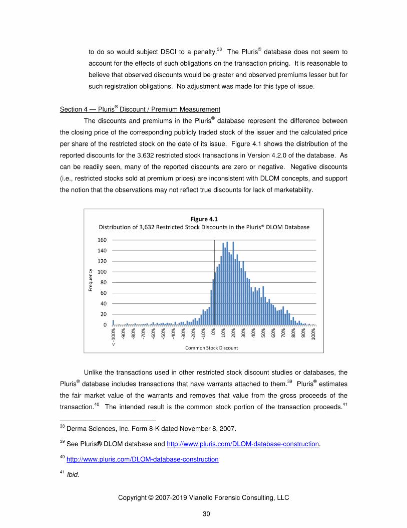
Section 4 — Pluris® Discount / Premium Measurement
The discounts and premiums in the Pluris® database represent the difference between
the closing price of the corresponding publicly traded stock of the issuer and the calculated price
per share of the restricted stock on the date of its issue. Figure 4.1 shows the distribution of the
reported discounts for the 3,632 restricted stock transactions in Version 4.2.0 of the database. As
can be readily seen, many of the reported discounts are zero or negative. Negative discounts
(i.e., restricted stocks sold at premium prices) are inconsistent with DLOM concepts, and support
the notion that the observations may not reflect true discounts for lack of marketability.
Unlike the transactions used in other restricted stock discount studies or databases, the
Pluris® database includes transactions that have warrants attached to them.
39 Pluris
® estimates
the fair market value of the warrants and removes that value from the gross proceeds of the
transaction.40
The intended result is the common stock portion of the transaction proceeds.41
38
Derma Sciences, Inc. Form 8-K dated November 8, 2007. 39
See Pluris® DLOM database and http://www.pluris.com/DLOM-database-construction. 40
http://www.pluris.com/DLOM-database-construction 41
Ibid.
0
20
40
60
80
100
120
140
160
< -
10
0%
-90
%
-80
%
-70
%
-60
%
-50
%
-40
%
-30
%
-20
%
-10
%
0%
10
%
20
%
30
%
40
%
50
%
60
%
70
%
80
%
90
%
10
0%
Fre
qu
en
cy
Common Stock Discount
Figure 4.1
Distribution of 3,632 Restricted Stock Discounts in the Pluris® DLOM Database

Copyright © 2007-2019 Vianello Forensic Consulting, LLC 31
Instead of using Black-Scholes or other option models, Pluris® uses its LiquiStat™ data to
determine the value of restricted stock private placement transactions with warrants.42
Pluris®
states that it is its opinion that Black-Scholes and other theoretical models overvalue warrants.43
Of the 3,632 transactions in the Pluris® database, 1,867 had warrants attached,
representing 51% of the transactions in the database. Of the 3,189 transactions reporting
discounts greater than zero, 1,760 (55%) had warrants attached. Table 4.1 shows that there is a
material difference in average restricted stock discounts depending on whether warrants attach to
the transactions.
Table 4.1
All Transactions With Warrants Without Warrants
Restricted Stock Discount Count Average Discount Count
Average Discount Count
Average Discount
All transactions 3,632 22.4% 1,867 30.3% 1,765 14.0%
Discounts > Zero 3,189 28.4% 1,760 33.6% 1,429 22.0%
The average discount for the 3,632 restricted stock transactions comprising the entire
Pluris® database is 22.4%. Reducing the population to the 3,189 transactions with reported
discounts that are greater than zero increased the average discount to 28.4%. Further
investigation revealed that the reported discounts for transactions involving warrants are
dramatically greater than for transactions without warrants. Looking only at the transactions with
reported discounts greater than zero, we found that those with warrants reported an average
discount of 33.6% compared to 22.0% for the transactions without warrants—53% more discount.
The dichotomy of warrant and warrantless transactions is an example of how other
factors can affect the amount of the discount. For example, LiquiStat may undervalue the portion
of the transaction value attributable to the warrants, thereby inflating the supposed restricted
stock discount;44
or transactions with warrants may represent riskier stocks or other factors that
require greater compensation for the investor; or perhaps warrants should be considered
valueless, which would further increase the restricted stock discount; or perhaps the warrant has
a much higher value than Pluris® estimated, reducing the restricted stock discount. Furthermore,
42
Ibid. 43
Ibid. 44
Undervaluing warrants decreases the portion of the discount attributed to the warrant while increasing the portion attributed to the restricted stock, thereby increasing the reported restricted stock discount.

Copyright © 2007-2019 Vianello Forensic Consulting, LLC 32
the discrepancy in discounts between transactions with and without warrants may differ from
industry-to-industry, time, and other factors. It would be prudent for practitioners to investigate
the value of any warrants attached to restricted stock transactions before relying on them or the
Pluris® discount percentages. Alternatively, it may be prudent to exclude transactions with
warrants from one's DLOM analysis. It is beyond the scope of this practice aid to test values that
Pluris® assigned to warrants; the reported Pluris
® discounts are therefore taken at face value for
the analyses described in this paper.
Section 5 — Discount Correlation with Total Assets, Market Value-to-Book Value Ratio, 12-Month Stock Price Volatility, Percentage of Shares Outstanding, and Calendar Quarters to Sell
A June 5, 2010, presentation45
by Pluris® to the National Association of Certified
Valuators and Analysts (NACVA) included several graphs (shown below) that suggest a strong
association between the restricted stock discounts reported in the Pluris® database and certain
underlying transactional metrics. Those metrics are total assets; market value-to-book value
ratio; 12-month stock price volatility for the publicly traded stock; block size of the restricted stock
as a percentage of shares outstanding; and block size (quarters to sell). The strength of the
associations is tested in the subsections below after grouping the discounts reported in the
Pluris® database into size-based deciles—the same method employed by Pluris
®.
Section 5.A Discounts and Block Size
The presumption is that block size is an indicator of the illiquidity of the shares sold in the
private placement because the largest blocks are very hard to trade out of after the placement
and would tend to be viewed by most buyers as more akin to private equity than public equity that
is temporarily restricted.46
The presumption can be tested by comparing discounts and the
percentage of shares outstanding represented by a block of stock. Figure 4.2 shows that a
strong R-squares of correlation results when the discounts of the restricted stock transactions
reported in the database are grouped into size-based deciles according to the percentage of
shares outstanding.
The positive association between percentage-block size and restricted stock discount is
somewhat illogical. Considering that the companies comprising the Pluris® database are publicly
traded, one could reasonably conclude that corporate control increases as the percentage of
outstanding shares represented by the block size increases. Given that controlling interests are
considered to be easier to sell than minority interests, the relationship of observed discounts to
block size should be negative, not positive.
46
http://www.pluris.com/files/PDFs/Pluris_DLOM_Database_Demo.pdf, slide 18.

Copyright © 2007-2019 Vianello Forensic Consulting, LLC 33
Applying the regression formulas to assumptions of 1% and 100% blocks of shares
outstanding results in implied discounts from 9.1% to 63.7% depending on the regression formula
used as per Table 4.2. It is incongruous that the projected discount range is so different between
the two formulas considering that the R-squares of correlation of the linear and logarithmic
regressions are so closely aligned. It would be difficult, if not impossible, to state whether a 100%
owned private company should have a 35% or a 64% DLOM based solely on this information.
Contrary to the presumption underlying the block size analysis is the fact that the Pluris®
database includes 517 transactions with stock discounts of 50% or greater for which the average
percentage block size is just 18% of shares outstanding. This fact, lost by grouping the data in
deciles, suggests that discounts do not increase with block size.
Table 4.2
Implied Range of Discounts Based on Pluris® Deciles of Blocks of Stock as a
Percentage of Shares Outstanding 1% of Shares Outstanding 100% of Shares Outstanding Linear Regression y = 0.4787x + 0.158
16.3%
63.7%
Logarithmic Regression y = 0.0574ln(x) + 0.3532 9.1% 35.3%
The block size presumption can also be tested by grouping the discounts of the reported
restricted stock transactions according to the number of calendar quarters required to sell the
block of stock under the SEC Rule 144 "dribble out" provision. This comparison is complicated
by the fact that the number of quarters reported is very high for many of the transactions in the
0%
5%
10%
15%
20%
25%
30%
35%
0%
5%
10%
15%
20%
25%
30%
35%
40%
1 2 3 4 5 6 7 8 9 10
Av
era
ge
Plu
ris
Dis
cou
nt
Blo
ck S
ize
(%
of
Sh
are
s O
uts
tan
din
g)
Deciles
Block Size (% of Shares Outstanding) Average Pluris Discount
Figure 4.2
Discounts Based on Percentage of Shares Outstanding
R² = 85.6% (linear)
R² = 83.3% (logarithmic)

Copyright © 2007-2019 Vianello Forensic Consulting, LLC 34
Pluris® database. Figure 4.3A shows that according to Pluris
® the average 10th decile transaction
requires 660 quarters to liquidate the position. Moreover, the discounts associated with the
transactions with much longer purported periods of illiquidity seem illogically low. An asset that
cannot be sold for years should have a 100% DLOM at some point. The fact that the average
discount of the ninth and 10th decile transactions does not approach 100% is an indication that
the discounts do not exclusively reflect illiquidity. Or it may be that the presumption that
discounts are associated with the dribble out provision is defective because it ignores that a sale
of the entire block could be made in a private transaction in a potentially much shorter period of
time. It is therefore not unreasonable to conclude that SEC Rule 144 dribble out time periods are
not appropriate indicators of DLOM for blocks of restricted stocks that will require long time
periods for selling into the public markets absent some provision that prohibits or limits sale of the
block in non-public transactions.
Figure 4.3A indicates a weak 42.0% linear R-square of correlation between deciles of
reported discounts and Rule 144-based time periods. But when the data is considered
logarithmically, as in Figure 4.3B, the analysis indicates a strong 82.1% R-square of correlation—
virtually double the linear regression result.
2.1x 4.9x 7.3x 10.1x 13.0x 16.2x 19.2x 24.8x40.4x
660.6x
12%
27%
0%
5%
10%
15%
20%
25%
30%
35%
0
100
200
300
400
500
600
700
1 2 3 4 5 6 7 8 9 10
Ave
rag
e P
luri
s D
isco
un
t
Blo
ck S
ize
(Q
ua
rte
rs t
o S
ell)
Block Size Quarters to Sell Average Pluris Discount
Figure 4.3A
Discounts Based on Quarters to Sell
R² = 42.0%

Copyright © 2007-2019 Vianello Forensic Consulting, LLC 35
Table 4.3 shows the range of discounts implied by applying the logarithmic regression
formula to time periods equal to 1 calendar quarter and 660 calendar quarters. It is illogical that
the discount for a required holding period of one calendar quarter should be about 13% while the
discount for a required holding period of 165 years should be just 34%.
Table 4.3
Implied Range of Discounts Based on Pluris® Deciles of the Number of Calendar Quarters
Needed to Sell a Block of Stock Applying Rule 144 1 Quarter to Sell 660 Quarters to Sell Logarithmic Regression y = 0.0324ln(x) + 0.1319
13.2%
34.2%
Figures 4.3A and 4.3B display obvious extreme skewing of the 10th decile time periods.
Figure 4.3C shows that excluding the 10th decile makes only a negligible change the R-square—
three hundredths of a percent. The R-square of correlation per Figure 4.3B is 82.12% while per
Figure 4.3C it is 82.09%.
y = 0.0324ln(x) + 0.1319
R² = 0.8212
0%
5%
10%
15%
20%
25%
30%
35%
40%
0.0x 100.0x 200.0x 300.0x 400.0x 500.0x 600.0x 700.0x
Figure 4.3B
Logarithmic Regression of Discounts and Quarters to Sell
Ave
rag
eD
isco
un
t p
er
De
cile
Average Number of Calendar Quarters to Sell the Block of Stock

Copyright © 2007-2019 Vianello Forensic Consulting, LLC 36
Excluding the 10th decile of transactions changes the regression formula in a way that
results in the broader range of predicted results shown in Table 4.4 compared to Table 4.3.
Whether the 10th decile transactions are included or excluded, however, one must question
basing DLOM conclusions on the metric of Rule 144 calendar quarters. It seems unreasonable to
conclude that a holding period of 165 years would result in a discount of just 34% to 40%.
Something much closer to 100% seems appropriate.
Table 4.4
Implied Range of Discounts Based on Nine Pluris®
Deciles of the Number of Calendar Quarters Needed to Sell a Block of Stock Applying Rule 144
(Omits the 10th
Decile) 1 Quarter to Sell 660 Quarters to Sell Logarithmic Regression y = 0.0465ln(x) + 0.1003
10.0%
40.2%
The above analyses of discounts based on decile groupings of the percent of shares
outstanding seem to support a presumption that block size is an indicator of the illiquidity of the
shares sold in the private placement, despite being somewhat illogical. But the increasing
discounts associated with increasing percentage-block sizes could easily be attributable to
additional or alternative causes. Possible explanations of the discounts may be investor
negotiating strength as the size of the block increases, issuer compulsion, other forms of
compensation granted by the issuer to the investor, the industry of the issuer, or other factors.
Practitioners would be right to question the reasonableness of basing discount and DLOM
y = 0.0465ln(x) + 0.1003
R² = 0.8209
0%
5%
10%
15%
20%
25%
30%
0.0x 5.0x 10.0x 15.0x 20.0x 25.0x 30.0x 35.0x 40.0x 45.0x
Figure 4.3C
Logarithmic Regression of Discounts and Quarters to Sell without the 10th Decile
Ave
rag
eD
isco
un
t p
er
De
cile
Average Number of Calendar Quarters to Sell the Block of Stock

Copyright © 2007-2019 Vianello Forensic Consulting, LLC 37
conclusions on the percentage of shares outstanding that is represented by a block of stock
because of the possible logical disconnection.
Section 5.B Firm Size Comparisons
Many investors will accept the premise that the size of an enterprise is an indicator of its
riskiness and investment attractiveness. Risk is believed to be lower for larger firms.
Correspondingly, the presumption is that smaller companies require significantly deeper
discounts than larger companies. Indeed, Figure 4.4A bears this presumption out. It shows that
a strong 84.8% logarithmic R-square of correlation results when the discounts of the restricted
stock transactions reported in the Pluris® database are grouped into size-based deciles according
to total assets.
Figure 4.4A shows that the 10th decile companies are very large. Omitting the 10th
decile from the analysis increased the R-square of correlation 92.1%. However, reliability
requires correlations to be reasonably consistent across the full body of data that includes the
10th decile, so the approach of excluding the 10
th decile simply because the asset values are
large is rejected.47
Nevertheless, the reported total assets seem to provide a strong explanation
of the variation in the observed discounts, which tentatively supports using total assets to predict
discounts.
47
The R-square of correlation using linear regression is a weak 33.5%. Omitting the 10th decile
transactions are omitted from the analysis increased the R-square of linear correlation to 59.7%. However, as stated, reliability requires correlations to be reasonably consistent across the full body of data without arbitrary exclusions, so the approach of excluding the 10
th decile is again
rejected.
0%
5%
10%
15%
20%
25%
30%
35%
40%
$1
$10
$100
$1,000
$10,000
$100,000
1 2 3 4 5 6 7 8 9 10
Ave
rag
e P
luri
s D
isco
un
t
To
tal A
sse
ts (
Mill
ion
s)
Total Assets Average Pluris Discount
Figure 4.4A (y =Logarithmic Scale)
Discounts Based on Deciles of Total Assets
R² = 84.8% (logarithmic)

Copyright © 2007-2019 Vianello Forensic Consulting, LLC 38
Figure 4.4B presents the logarithmic regression of the data shown in Figure 4.4A. Note
that the relationship is virtually a straight line declining from approximately 33% discount for the
smallest companies to 0% discount for the largest companies. Table 4.5 presents the range of
discounts predicted by the regression formula shown in Figure 4.4B.
Table 4.5 Implied Range of Discounts Based on Pluris
® Deciles Total Assets
$100,000 of Total Assets $24.2 Billion of Total Assets
Logarithmic Regression y = -0.033ln(x) + 0.3331 40.9% 0.0%
Many practitioners may find a 40% DLOM implied for very small companies to be
reasonable. But what if the assets of the small firm is cash or some other highly liquid asset? Or
what if the assets are time shares? Should the DLOM still be 40% under those circumstances?
Logic suggests otherwise. Likewise, the zero DLOM implied for very large companies suggests
that there should be little or no price risk associated with an illiquid marketing period. The
volatility of the stock market—even for very large companies—contradicts this notion. These
considerations undermine the use of discounts based on total assets as a benchmark for DLOM
estimation. Nevertheless, logarithmic analysis of discounts on the decile groupings of total assets
supports a conclusion that size is an indicator of riskiness and investment attractiveness.
Section 5.C Balance Sheet Strength
Many investors will accept the premise that the balance sheet strength of an enterprise is
an indicator of its riskiness and investment attractiveness. Issuers with weaker balance sheets
y = -0.033ln(x) + 0.3331
R² = 0.8477
0%
5%
10%
15%
20%
25%
30%
35%
40%
$0 $1 $10 $100 $1,000 $10,000 $100,000
Figure 4.4B
Logarithmic Regression of Discounts and Total Assets
Total Assets (Millions)
Ave
rag
e P
luri
s D
isco
un
t

Copyright © 2007-2019 Vianello Forensic Consulting, LLC 39
presumably require deeper discounts. Some investors associate the ratio of market value-to-
book value with balance sheet strength, and assume that higher multiples are a sign of financial
weakness. But the ratios do not necessarily describe the financial strength of enterprises’ highly
appreciated asset values. Mining, real estate-heavy, and many technology companies come to
mind in this regard. Instead of being a sign of balance sheet weakness, market value-to-book
value ratios can be a sign of strength to the extent that the ratio is a measure of investors’
expectations regarding the effectiveness with which a business can generate profits from its
assets. In such situations higher ratios are an indication of superior performance expectations
(financial growth) that come from stronger business plans, more valuable assets, stronger market
positions, stronger management, and/or other strength factors. Nevertheless, market value-to-
book value ratios appear to be a predictor of the restricted stock discounts reported in the Pluris®
database. Grouping the transaction discounts reported in the database into deciles according
ranking by market value-to-book value ratio yields a modest R-square of correlation of 56.9% as
Figure 4.5A shows.
Although it is intuitive that balance sheet strength is an indicator of riskiness and
investment attractiveness, and that issuers with weaker balance sheets require significantly
deeper discounts, a 56.9% R-square of correlation leaves a lot of "noise" unaccounted for.
Logarithmic regression provides a better answer to the question, resulting in the very high 96.0%
R-square of correlation shown in Figure 4.5B.
0%
5%
10%
15%
20%
25%
30%
35%
0
10
20
30
40
50
1 2 3 4 5 6 7 8 9 10
Ave
rag
e P
luri
s D
isco
un
t
Ma
rke
t-to
-Bo
ok
Ra
tio
MTB Ratio Average Pluris Discount
Figure 4.5A (Linear Scale)
Discounts Based on "Market Value to Book Value Ratios"
R² = 56.9%

Copyright © 2007-2019 Vianello Forensic Consulting, LLC 40
We can conclude from Figure 4.5B that (1) market value-to-book value ratios are a strong
predictor of restricted stock discounts (regardless of whether the ratio indicates balance sheet
"strength," and (2) the relationship between market value-to-book value and restricted stock
discounts is logarithmic and not linear. But the regression line of Figure 4.5B implies a ceiling for
discounts despite no apparent ceiling on the market value-to-book value ratio. Table 4.6 shows
that the implied discount for a company with a market value-to-book value ratio of 1000:1 is
54.3%. This seems unreasonably low given a premise that such a ratio represents a very
financially weak enterprise.
Table 4.6
Implied Range of Discounts Based on Pluris® Deciles of Market-to-Book Value Ratio
1x Ratio 1000x Ratio Logarithmic Regression y = 0.0643ln(x) + 0.0991
9.9%
54.3%
Section 5.D Stock Price Volatility
Stock price volatility is a direct measure of the risk associated with a stock. One would
accordingly expect a strong association between the price volatility of the publicly traded stock of
a restricted stock issuer and the negotiated transaction discounts. This expectation was tested
by creating decile groupings of the discounts reported in the Pluris® database according to the
reported 12-month price volatilities. Figure 4.6A shows a 58.4% R-square of correlation using
linear regression that, as with the market value-to-book value ratio linear regression analysis,
leaves a lot of "noise" unaccounted for.
y = 0.0643ln(x) + 0.0991
R² = 96.0%
0%
5%
10%
15%
20%
25%
30%
35%
40%
- 10 20 30 40 50
Figure 4.5B
Logarithmic Regression of Discounts and Market-to Book Value Ratio
Ave
rag
e D
isco
un
t p
er
De
cile
Market Value-to-Book Value Ratio by Decile

Copyright © 2007-2019 Vianello Forensic Consulting, LLC 41
Figure 4.6B considers the same data using logarithmic regression. Again, as with the
market value-to-book value ratio analysis, the statistical relationship improves dramatically—to an
86.4% R-square of correlation in this instance. Based on the decile analysis at least, stock price
volatility appears to strongly influence restricted stock discounts.
We can conclude from Figure 4.6B that (1) stock price volatilities are a strong predictor of
restricted stock discounts, and (2) the relationship between price volatility and restricted stock
discounts is logarithmic and not linear. But the regression line of Figure 4.6B implies a ceiling for
0%
5%
10%
15%
20%
25%
30%
35%
0%
50%
100%
150%
200%
250%
300%
350%
1 2 3 4 5 6 7 8 9 10
Av
era
ge
Plu
ris
Dis
cou
n t
Pri
ce V
ola
tili
ty
Deciles
Price Volatility Average Pluris Discount
Figure 4.6A (Linear Scale)
Average Pluris Observed Discounts v. Average Price Volatility
R² = 58.4%
y = 0.0939ln(x) + 0.2336
R² = 86.4%
0%
5%
10%
15%
20%
25%
30%
35%
40%
0% 50% 100% 150% 200% 250% 300% 350%
Figure 4.6B
Logarithmic Regression of Discounts and Stock Price Volatility
Ave
rag
e D
isco
un
t p
er
De
cile
Stock Price Volatility by Decile

Copyright © 2007-2019 Vianello Forensic Consulting, LLC 42
discounts that seems inconsistent with very high price volatility situations. Table 4.7 shows that
the implied discount for a company with a price volatility of 1000% is just 45.0%. This again
seems unreasonably low.
Perhaps not illogically, the price volatility regression formula implies a price premium for
very low price volatility stocks. Table 4.7 shows an implied 19.9% premium for companies with
1% price volatility.
Table 4.7 Implied Range of Discounts Based on Pluris
® Deciles of Price Volatility
1% Price Volatility 1000% Price Volatility Logarithmic Regression y = 0.0939ln(x) + 0.2336
(19.9)%
45.0%
Section 5.E Testing Statistical Significance
The correlations of block size (percentage of shares outstanding and quarters to sell),
total assets, market-to-book value, and annual stock price volatility were tested for statistical
significance. This was a two-part test. The first part involved identifying the 2,496 restricted
stock transactions in the Pluris® database for which positive values are reported for all five of the
metrics. The second part involved identifying the 1,162-transaction subset of the 2,496-
transaction group that does not have warrants attached.
Table 4.8 shows that four of the five metrics passed the significance test; only the total
assets metric failed. The variable that was most strongly significant is stock price volatility,
which suggests that the restricted stock price negotiators were particularly sensitive to the price
risks associated with the stocks. The market-to-book value ratio was the second strongest
variable, which is not surprising considering that stocks with high ratios have substantial “blue
sky,” which often adds to stock price volatility. Importantly, this analysis contradicts the
assumption that DLOM conclusions should be based on the total assets of a business.
Table 4.8
2,496 Transactions Positive Value Variables
1,162 Transactions Positive Values without Warrants
Independent Variable R Square t Stat P-value Significant? R Square t Stat P-value Significant?
Block Size (Shares Outstanding) 4.3% 10.57024 0.00000 Yes 6.4% 8.91435 0.00000 Yes
Block Size (Quarters to Sell) 0.3% 2.84111 0.00453 Yes 1.0% 3.35573 0.00082 Yes
Total Assets (Latest Quarter) 0.1% -1.76321 0.07799 No 0.1% -1.31879 0.18750 No
Market to Book Ratio 8.7% 15.42419 0.00000 Yes 11.2% 12.08104 0.00000 Yes
Annual Stock Price Volatility 25.0% 22.17967 0.00000 Yes 23.8% 19.03871 0.00000 Yes

Copyright © 2007-2019 Vianello Forensic Consulting, LLC 43
Section 6 — The Discounts Reported in the Pluris® DLOM Database
™ Are Not Consistent with
Past Changes in SEC Rule 144 Required Holding Periods
As discussed in Section 5, the “quarters to sell” metric reported in the Pluris® database
offers a statistically significant explanation of the changes in the observed discounts.
Consideration is now given to whether changes in the SEC Rule 144 required holding period
offers an additional explanation of restricted stock transaction discounts reported in the database.
The original Rule 144 required that restricted stocks be held for two years past the issue date
before they could be “dribbled out” into the public marketplace. The SEC changed the required
holding period to one year effective April 29, 1997, and to six months effective February 15,
2008.48
None of the transactions in Version 4.2.0 of the Pluris® database predates April 29, 1997,
so the large holding period change from two years to one year cannot explain any of the changes
in the reported restricted stock discounts.
Conventional wisdom, supported by several restricted stock studies, is that smaller
restricted stock discounts have resulted from the successive changes in Rule 144 holding
period.49
A reduction in discount is logical when the restriction goes from two years to one year to
six months, because the restricted block of stock can be liquidated quicker. The restricted stock
studies by Columbia Financial Advisors confirmed this market reaction. See Table 3.1 in Chapter
3. Quickness of sale (i.e., increased liquidity) evidently reduces holding period risk.
Table 4.9 summarizes the transactions reported in the Pluris® database based on issue
dates before and after the SEC’s November 15, 2007, announcement date of the change from a
one-year to a six-month required holding period. The announcement date is the appropriate
demarcation because the rule change was applicable to stocks acquired both before and after the
February 15, 2008, effective date.50
It is assumed that negotiators of a restricted stock
transaction would have known of the rule change upon the announcement by the SEC.
Table 4.9
Transactions with Discounts Greater than Zero
Issue Date Restriction
Period
All 3,632 Transactions 3,189 Transactions 1,429 Transactions without Warrants
Count Discount Count Discount Count Discount
1/2/2001 – 11/14/2007 1 Year 2,379 23.0% 2,160 27.6% 936 21.7% 11/15/2007 – 6/30/2014 6 Months 1,253 21.2% 1,029 30.0% 493 22.5%
48
“Discount for Lack of Marketability Job Aid for IRS Valuation Professionals – September 25, 2009,” p 15. 49
Ibid, p 17. 50
https://www.sec.gov/rules/final/2007/33-8869.pdf

Copyright © 2007-2019 Vianello Forensic Consulting, LLC 44
Table 4.9 demonstrates that the average observed discount for all transactions in the
Pluris® database decreased slightly from 23.0% to 21.2% upon the announcement that the Rule
144 holding period would change from one year to six months. But the opposite is observed
when only transactions with positive discounts (i.e., common stock discounts greater than zero)
are included. For the latter set, the average discounts reported by Pluris® increased from 27.6%
to 30.0% for one-year and six-month restriction periods, respectively. And the same occurred for
the subset of transactions that did not include warrants. The average discount for warrantless
transactions increased from 21.7% before the announcement date to 22.5% after the
announcement date. These results are contrary to expectations.
The restricted stock discounts observed in the Pluris® database do not seem to behave
consistently with the conventional wisdom regarding the effect of Rule 144 time restrictions.
Therefore, one must consider that one or more things other than Rule 144 holding periods explain
the discounts reported in the database. A reasonable explanation is that the negotiators of
restricted stock transactions of the size comprising the database anticipate block sales instead of
dribble-out sales of their holdings.
Section 7 — Correlation of the Pluris® Restricted Stock Discounts Valuation Metrics
Pluris® database reports 76 fields of data for each restricted stock transaction. Sixty-two
of those fields might be considered valuation metrics. Linear regression was initially used to
calculate the R-squares of correlation and regression formula slopes for these 62 metrics relative
to the discounts reported by Pluris®. The results are presented in Table 4.10. The lines
presented in red are the metrics used in the Pluris® DLOM calculator, except for price volatility.
Table 4.10 shows that none of the metrics exhibits a large R-square of correlation with
transaction discounts, and few exhibit a regression line slope that is not essentially flat. Flat
regression lines offer no predictive power.
The largest correlations occurred with the transactions for which price volatility was
reported and that have discounts greater than zero. These R-squares of correlation range from
8.9% to 12.4%, and have very shallow, but positive, regression line slopes that range from
0.0588:1 to 0.0879:1. The best performing metric in the linear regression analysis was 12-month
daily price volatility, with an R-square of 12.4%. This metric explains about an eighth of the
variation in discounts reported in the database. Obviously, practitioners would prefer to see R-
squares that are closer to 100%.
It seems unreasonable to benchmark a restricted stock DLOM on even the strongest
correlations reported in Table 4.10. Benchmarking DLOMs on the even more poorly correlated
parameters used in the Pluris® DLOM calculator seems problematic.

Copyright © 2007-2019 Vianello Forensic Consulting, LLC 45
Table 4.10
Linear Regressions of Pluris® DLOM Database Financial Metrics with the Observed Discounts
All 3,632 Transactions
3,189 Transactions with
Discounts Greater than Zero
R2 Slope R
2 Slope
Price Volatility Data Daily volatility over 12 months 2.7% 0.0470 12.4% 0.0641 Daily volatility over 12 months or applicable period prior
to issue date 3.0% 0.0445 12.4% 0.0588 Daily volatility over six months 2.1% 0.0450 12.0% 0.0709 Weekly volatility over 12 months 3.5% 0.0753 11.9% 0.0864 Weekly volatility over six months 2.9% 0.0695 11.2% 0.0879 Daily volatility over three months 2.1% 0.0435 11.0% 0.0662 Weekly volatility over three months 2.7% 0.0560 8.9% 0.0653
Price Data Effective purchase price per share 3.1% (0.0056) 10.2% (0.0067) Purchase price 2.9% (0.0054) 9.9% (0.0066) Closing price on announcement date (A+0) 2.1% (0.0047) 9.2% (0.0067) Closing price three days after announcement date (A+3) 2.1% (0.0047) 9.2% (0.0066) Exercise Price 2.6% (0.0102) 8.3% (0.0132) Closing price 10 days after issue date (C+10) 1.4% (0.0035) 7.2% (0.0050) Closing price seven days after issue date (C+7) 1.5% (0.0035) 7.1% (0.0050) Closing price seven days prior to issue date (C-7) 1.5% (0.0035) 7.1% (0.0050) Volume-weighted average price 10 days prior to issue
date (VWAP) 1.4% (0.0035) 7.1% (0.0050) Closing price three days after issue date (C+3) 1.4% (0.0034) 7.0% (0.0050) Closing price one day after issue date (C+1) 1.4% (0.0034) 6.8% (0.0049) Closing price one day prior to issue date (C-1) 1.3% (0.0034) 6.8% (0.0049) Closing price on the issue date (C+0) 1.3% (0.0033) 6.7% (0.0049)
Restricted Stock Data Fair market value per warrant 1.6% (0.0254) 6.7% (0.0377) Number of warrants 1.9% 0.0000 6.3% 0.0000 Block size (shares outstanding) 2.4% 0.4692 3.9% 0.3929 Shares sold 0.9% 0.0000 3.2% 0.0000 Gross proceeds 0.2% (0.0000) 0.8% (0.0000) Common stock portion of proceeds 0.3% (0.0000) 0.8% (0.0000) Warrants portion of gross proceeds 0.4% 0.0000 0.0% 0.0000 Block Size (Volume) 0.0% (0.0000) 0.3% 0.0000
Block size (quarters to sell) 0.0% (0.0000) 0.4% 0.0000 Issue date 0.0% 0.0000 0.5% 0.0000 Placement ID number 0.0% (0.0000) 0.4% 0.0000
Financial and Market Data Market-to-book ratio 4.6% 0.0040 8.7% 0.0036 Price divided by book value per share (P/BV) 4.6% 0.0040 8.7% 0.0036 Enterprise value divided by revenue for last 12 months
(EV/Revenue) 1.4% 0.0017 3.0% 0.0016 Dividend yield 0.9% (1.6625) 2.2% (1.9705) Net profit margin for last 12 months 1.0% (0.0995) 2.0% (0.0718)

Copyright © 2007-2019 Vianello Forensic Consulting, LLC 46
Revenue growth in 12 months prior to most recent 10-Q 0.3% (0.0345) 1.4% (0.0468) Price divided by average earnings per share for last 12
months (P/E) 0.1% (0.0003) 1.4% (0.0007) Shares outstanding 0.0% 0.0000 1.0% 0.0000 Market capitalization 0.2% (0.0000) 0.8% (0.0000) Price divided by the estimated average earnings per
share for the next two years (P/E FY+2) 1.3% 0.0009 0.6% 0.0005 Total equity on most recent 10-Q 0.2% (0.0000) 0.5% (0.0000) Total revenues 12 months prior to most recent 10-Q 0.2% (0.0000) 0.5% (0.0000) Beta relative to S&P 500 for 12 months prior to issue
date 0.2% (0.0001) 0.5% (0.0001) Trading volume over twelve months or applicable period 0.9% (0.0000) 0.4% (0.0000) Trading volume multiplied by the issuer's closing stock
price on issue date 0.1% (0.0000) 0.4% (0.0000) Average daily trading volume over 12 months prior to
issue date 0.8% (0.0000) 0.4% (0.0000) Expiration Date 0.2% 0.0000 0.2% 0.0000 Average daily trading volume over six months prior to
issue date 1.1% (0.0000) 0.2% (0.0000) VIX as of the issue date 0.7% (0.3533) 0.2% (0.1261) Z-score 0.1% (0.0000) 0.2% (0.0000) Enterprise value 0.0% (0.0000) 0.2% (0.0000)
SEC Filing Data Total debt on most recent 10-Q 0.0% (0.0000) 0.1% (0.0000) Average daily trading volume over three months prior to
issue date 1.0% (0.0000) 0.1% (0.0000) Total assets on most recent 10-Q 0.0% (0.0000) 0.1% (0.0000) Average daily trading volume over one month prior to
issue date 0.7% (0.0000) 0.1% (0.0000) Total liabilities on most recent 10-Q 0.0% (0.0000) 0.1% (0.0000) EBITDA 12 months prior to most recent 10-Q 0.0% (0.0000) 0.1% (0.0000) Average daily trading volume over seven days prior to
issue date 0.1% (0.0000) 0.1% (0.0000) Price divided by the estimated average earnings per
share for the next year (P/E FY+1) 0.2% 0.0003 0.0% 0.0001 Pre-tax income 12 months prior to most recent 10-Q 0.0% (0.0000) 0.0% (0.0000) Net income 12 months prior to most recent 10-Q 0.0% (0.0000) 0.0% (0.0000)
Using the transactions reported in the Pluris® database, Table 4.11 summarizes the
average (mean), standard deviation, and the coefficient of variation for each of eight valuation
parameters comprising the Pluris® DLOM calculator. All of the metrics except net profit margin
and market value-to-book value ratio exhibit very large coefficients of variation, ranging as high
as 36.2:1 for total assets. In comparison, the coefficients of variation shown for restricted stock
discounts are 0.7:1. The high coefficients of variation of most of the Pluris® DLOM calculator
parameters undermine their predictive utility for DLOM estimation. Net profit margin (1.9
coefficient of variation) and market value-to-book value ratio (1.4 coefficient of variation) appear
to be more meaningful for DLOM estimation. Twelve-month price volatility, with a coefficient of
variation of .9 to 1 most closely approximates the data distribution of the restricted stock

Copyright © 2007-2019 Vianello Forensic Consulting, LLC 47
discounts. This is consistent with the higher logarithmic R-squares of correlation that price
volatility exhibits with restricted stock discounts as shown in Table 4.11.
Table 4.11
Financial Parameters Used in the Pluris® DLOM Calculation Methodology
All 3,632 Transactions 3,189 Transactions with Discounts > Zero
Average Standard Deviation
Coefficient of Variation Average
Standard Deviation
Coefficient of Variation
Pluris® DLOM Calculator Parameters
Total Assets $1,535,520,816 $55,612,171,960 36.2 $1,658,322,427 $59,281,730,272 35.7 Revenues 194,563,230 2,152,944,264 11.1 190,652,639 2,252,841,333 11.8 EBITDA 33,622,178 1,138,721,628 33.9 34,695,161 1,210,638,417 34.9 Net Income (9,182,288) 135,947,965 14.8 (9,006,978) 140,872,735 15.6 Net Profit Margin -16.7% 31.4% 1.9 -17.4% 31.8% 1.8 Total Equity 99,717,239 1,156,263,919 11.6 96,301,461 1,208,685,423 12.6 Enterprise Value 805,238,151 19,858,204,899 24.7 854,743,284 21,150,553,918 24.7 Market-to-Book Ratio 10.2 14.7 1.4 10.5 14.9 1.4
Comparative Parameters
12-Month Daily Price Volatility 124.2% 116.7% .9 124.5% 119.0% 1.0
Restricted Stock Discounts 22.4% 29.9% .7 28.4% 19.9% .7
Table 4.12 summarizes three transactional subsets of the Pluris® calculator metrics that
were analyzed using both linear and logarithmic regression. All of the subsets were limited to
those with positive discounts. Further limitations imposed were (1) transactions with stated
metric values (that is, not zero or blank); (2) transactions with only positive metric values; and (3)
transactions without warrants. Out of 3,632 transactions in the database, only 840 transactions
satisfied the first limitation, only 323 transactions satisfied the first two limitations, and only 253
transactions satisfied all three limitations. Logarithmic regression significantly improved the
regression results within the 840-transaction subset vis-à-vis linear regression, with the exception
of net profit margin subset. The 6.81% R-square of correlation for that metric is considered an
anomaly created by the presence of 517 transactions with negative net profit margins.

Copyright © 2007-2019 Vianello Forensic Consulting, LLC 48
Table 4.12
R-Squares of Correlation of Positive Discount Transaction Subsets of the Pluris® Database
Transactions With and Without Warrants Transactions Without
Warrants
840 with Non-Zero Metrics 323 with Positive Metrics 253 with Positive Metrics
Linear Logarithmic Linear Logarithmic Linear Logarithmic
Total Assets 0.26% 17.58% 0.42% 12.62% 0.41% 7.19%
Revenues 0.57% 10.32% 0.47% 4.09% 0.29% 0.74%
EBITDA 0.12% Neg.
Values 0.01% 6.64% 0.04% 2.78%
Net Income 0.24% Neg.
Values 0.33% 5.15% 0.11% 2.39%
Net Profit Margin 6.81% Neg.
Values 0.68% 0.29% 1.80% 1.80%
Total Equity 0.80% 16.34% 0.86% 10.84% 0.64% 6.68%
Enterprise Value 0.32% 11.83% 0.45% 7.03% 0.40% 2.98%
Market-to-Book Ratio 3.10% 5.99% 2.02% 6.91% 2.72% 6.98%
12-month daily volatility 16.07% 19.01% 21.34% 20.30% 26.72% 20.52%
Table 4.12 confirms that the restricted stock discounts reported in the database correlate
poorly on a linear basis with the parameters employed in the Pluris® calculator even with refined
data subsets. But that is not the case with price volatility, for which the refined subsets yield
linear and logarithmic R-squares of correlation improve with the dataset refinement.
Table 4.13 shows the R-squares of correlation of the Pluris® calculator parameters with
the restricted stock discounts reported in the Pluris® database. Explanatory power increases
somewhat as the group membership is narrowed from the 840 to 253. this is demonstrated by
the R-squares of correlation increasing from 20.89 to 29.1%. This may mean that DLOM
conclusions should not be based on parameters with negative values and that transactions with
warrants should be ignored.
Finally, the statistical significance of the Pluris® calculator parameters was considered for
the Table 4.12 subgroups. Table 4.13 shows that only price volatility is statistically significant
across all three subgroups, with t-Stats greater than +/- 2 and p-Values less than 0.05. The net
profit margin metric is statistically significant for the 840 and 253-transaction groups. The market
value-to-book value metric is statistically significant for the 840-transaction group. None of the
other Pluris® calculator parameters are statistically significant for any of the three subgroups of
transactions.

Copyright © 2007-2019 Vianello Forensic Consulting, LLC 49
Table 4.13
R-Squares of Correlation of Positive Discount Transaction Subsets of the Pluris® Database
Transactions With and Without Warrants Transactions Without
Warrants 840 with Non-Zero
Metric Data 323 with Positive Metric
Data 253 with Positive Metric
Data
R-Square = 20.8% R-Square = 23.0% R-Square = 29.1%
t Stat P-value t Stat P-value t Stat P-value
Total Assets 1.339047 0.180922 0.699754 0.484601 0.481411 0.630658
Revenues -1.124144 0.261277 -0.909178 0.363956 -0.927224 0.354730
EBITDA 1.389704 0.164991 0.668319 0.504422 0.439243 0.660876
Net Income 1.601365 0.109677 1.169352 0.243152 1.391995 0.165197
Net Profit Margin -4.207082 0.000029 -1.341499 0.180731 -2.161333 0.031647
Total Equity -0.947467 0.343677 -0.991707 0.322106 -0.821767 0.412015
Enterprise Value -1.198804 0.230946 -0.583396 0.560047 -0.410644 0.681695
Market-to-Book Ratio 3.544787 0.000415 1.041203 0.298585 0.997442 0.319542
12-month daily volatility 10.513029 0.000000 8.155209 0.000000 8.278852 0.000000
The above analyses provide a reasonable basis to conclude that negotiators of restricted
stock transactions are much more concerned with the price volatility of the investment than with
other valuation metrics when pricing their transactions.
Section 8 — Using the Pluris® Database for Benchmarking
The limited number of transactions in the Pluris® database makes the identification of
appropriate benchmarks unlikely for most valuations. Although the database consists of 3,362
restricted stock transactions, there are only 2,085 unique issuers. Even the larger number is
likely to be insufficient for reasonable benchmarking. The transactions comprising the database
stretch over a period beginning January 2, 2001, and ending June 30, 2014—a period of 4,928
days. On average, there is less than one transaction per database day. Even if the number of
days is reduced to the approximate number of stock-trading days during the database period
(about 3,375 days), there are only 1.1 transactions per day on average.
Table 4.14 shows the percentage distribution of transactions in the Pluris® database.
About 58% of the potential valuation days have no transactional data. Table 4.14 also shows that
about 38% of all trading days have no transactional data.

Copyright © 2007-2019 Vianello Forensic Consulting, LLC 50
Table 4.14
Number of Pluris® Transaction Occurrences by Day
All Database Days Stock Trading Days Number of
Occurrences Number of Days Percent
Number of Days Percent
0 2,843 57.69% 1,290 38.23% 1 1,151 23.36% 1,151 34.10% 2 554 11.24% 554 16.41% 3 245 4.97% 245 7.26% 4 77 1.56% 77 2.28% 5 34 0.70% 34 1.00% 6 12 0.24% 12 0.36% 7 9 0.18% 9 0.27% 8 2 0.04% 2 0.06%
9 1 0.02% 1 0.03%
Total Days 4,928 100.00% 3,375 100.00%
Figure 4.7 shows the number of transactions in the database that occurred on the same
day. One day—December 30, 2005—had nine stock transactions. Two days had eight
transactions. Nine days had seven transactions. And so forth. No transactions are reported for
2,843 days in the 2001 to 2014 data range.
Figure 4.8 presents the distribution of transactions based on stock market trading days
shown in Table 4.14.
2,843
1,151
554
245
77
34
12
9
2
1
- 500 1,000 1,500 2,000 2,500 3,000
0
1
2
3
4
5
6
7
8
9
Figure 4.7
Number of Pluris Restricted Stock Transactions that Occurred on the Same Day
(from January 1, 2001 to June 27, 2014 - 4,926 total days)
Nm
be
ro
f T
ran
sact
ion
s O
ccu
rrin
g o
n t
he
Sa
me
Da
y
Number of Days with the Indicated Transction Occurrence Rate

Copyright © 2007-2019 Vianello Forensic Consulting, LLC 51
One problem represented by a small volume of transaction data is the likelihood that
none or only one transaction is reported for a particular valuation date. Another problem is the
reporting lag that occurs as the database is compiled. Before a transaction can be added to the
database, it must be reported by the issuer and then picked up by Pluris®. This imposes a
limitation on data availability for contemporary valuations. But it may be that practitioners can
compensate for the problems of too-limited of transaction data by selecting transactions that
occurred over a longer period than the one day represented by the valuation date. Of course, the
longer the time span required to capture the number of transactions that a practitioner may deem
sufficient, the more risk there is that economic circumstances may have materially changed
during the span.
Lack of comparability of the reported transactions to a valuation subject is another
problem associated with too little transactional data. The fewer the number of transactions, the
more work the analyst must likely do to establish comparability.
Moreover, it is problematic that nothing is known about how the transaction negotiators
actually priced their restricted stocks. Accordingly, there is a significant risk of appraisers failing
to consider the same things considered by the stock negotiators. Unlike the public marketplace
for which it can be presumed that investors’ decisions are based on publicly available information,
restricted stock pricing is a matter of private negotiation. It is speculation to assume that their
motivations align with any particular piece of information selected for benchmarking. It is further
problematic that narrowing transaction selection to seek comparability inhibits the ability to find
any potentially relevant transaction to use as a benchmark for a valuation subject.
38.23%
34.10%
16.41%
7.26%
2.28%1.01% 0.36% 0.27% 0.06% 0.03%
0%
5%
10%
15%
20%
25%
30%
35%
40%
45%
0 1 2 3 4 5 6 7 8 9
Figure 4.8
Probability of the Number of Transactions Occurring on a Stock Market Trading Date
Number of Transactions per Trading Day
Pe
rce
ng
ate
Occ
urr
en
ce
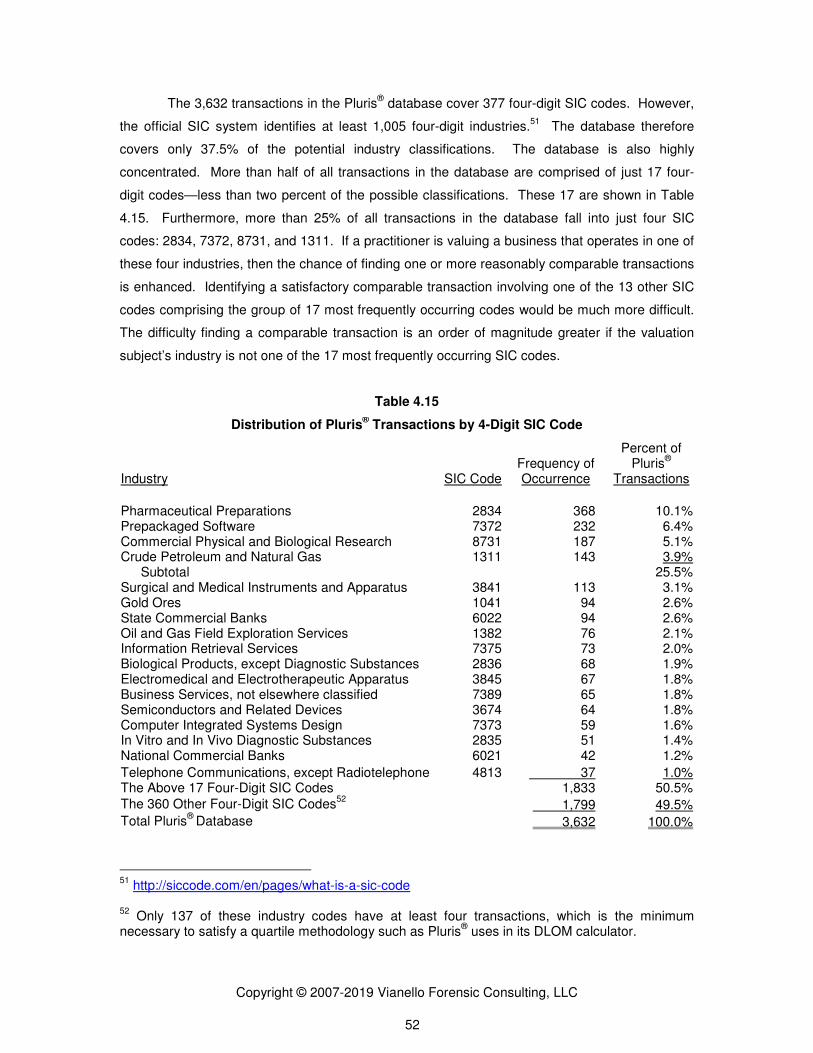
Copyright © 2007-2019 Vianello Forensic Consulting, LLC 52
The 3,632 transactions in the Pluris® database cover 377 four-digit SIC codes. However,
the official SIC system identifies at least 1,005 four-digit industries.51
The database therefore
covers only 37.5% of the potential industry classifications. The database is also highly
concentrated. More than half of all transactions in the database are comprised of just 17 four-
digit codes—less than two percent of the possible classifications. These 17 are shown in Table
4.15. Furthermore, more than 25% of all transactions in the database fall into just four SIC
codes: 2834, 7372, 8731, and 1311. If a practitioner is valuing a business that operates in one of
these four industries, then the chance of finding one or more reasonably comparable transactions
is enhanced. Identifying a satisfactory comparable transaction involving one of the 13 other SIC
codes comprising the group of 17 most frequently occurring codes would be much more difficult.
The difficulty finding a comparable transaction is an order of magnitude greater if the valuation
subject’s industry is not one of the 17 most frequently occurring SIC codes.
Table 4.15
Distribution of Pluris® Transactions by 4-Digit SIC Code
Industry SIC Code Frequency of Occurrence
Percent of Pluris
®
Transactions
Pharmaceutical Preparations 2834 368 10.1% Prepackaged Software 7372 232 6.4% Commercial Physical and Biological Research 8731 187 5.1% Crude Petroleum and Natural Gas 1311 143 3.9%
Subtotal 25.5% Surgical and Medical Instruments and Apparatus 3841 113 3.1% Gold Ores 1041 94 2.6% State Commercial Banks 6022 94 2.6% Oil and Gas Field Exploration Services 1382 76 2.1% Information Retrieval Services 7375 73 2.0% Biological Products, except Diagnostic Substances 2836 68 1.9% Electromedical and Electrotherapeutic Apparatus 3845 67 1.8% Business Services, not elsewhere classified 7389 65 1.8% Semiconductors and Related Devices 3674 64 1.8% Computer Integrated Systems Design 7373 59 1.6% In Vitro and In Vivo Diagnostic Substances 2835 51 1.4% National Commercial Banks 6021 42 1.2%
Telephone Communications, except Radiotelephone 4813 37 1.0% The Above 17 Four-Digit SIC Codes 1,833 50.5% The 360 Other Four-Digit SIC Codes
52 1,799 49.5%
Total Pluris®
Database 3,632 100.0%
51
http://siccode.com/en/pages/what-is-a-sic-code 52
Only 137 of these industry codes have at least four transactions, which is the minimum necessary to satisfy a quartile methodology such as Pluris
® uses in its DLOM calculator.

Copyright © 2007-2019 Vianello Forensic Consulting, LLC 53
The 17 four-digit codes represent 1,833 restricted stock transactions, ranging in count
from 368 transactions involving the pharmaceutical preparations industry to 37 transactions
involving the non-radio telephone communications industry. Industries falling outside of the top-
17 are represented by just five transactions on average; and 119 transactions have unique SIC
codes within the database. Coupled with the fact that the database covers a 13.5-year period, it
may be impossible to identify time-relevant transactions in the four-digit industry classification of a
valuation subject. Adding other elements of comparability to the benchmarking process greatly
exacerbates the task.
When practitioners are faced with an impossible task at an initially desired level of detail,
they often zoom out their analyses to base conclusions on a broader analytical view. With that in
mind the industry distribution of the Pluris® database was analyzed on a two-digit SIC code
basis.53
See Table 4.16. Just eight broad industries account for 2,546 (over 70%) of the 3,632
transactions in the database. The remaining 1,086 transactions are spread over 61 broad
industries—an average of less than 18 transactions per industry, and about one per nine months
of time range in the database.
Assuming a practitioner wanted to identify a single benchmark transaction from the four-
digit SIC code with the most transactions (Pharmaceutical Preparations, code 2834) for a single
53
As of this writing, there are 83 two-digit codes in the SIC system. Fourteen SIC codes are not represented in Version 4.2.0 of the Pluris
® DLOM database.
Table 4.16 Distribution of Pluris
® Transactions by 2-Digit SIC Code
Industry SIC
Code Occurrences Percent of
Transactions
Chemicals and Allied Products 28 591 16.3% Business Services 73 574 15.8% Measuring, Analyzing, And Controlling Instruments 38 298 8.2% Oil and Gas Extraction 13 262 7.2% Electrical and Other Electrical Equipment
and Components except Computer Equipment 36 235 6.5%
Engineering, Accounting, Research, Management, and Related Services 87 214 5.9% Metal Mining 10 198 5.5%
Depository Institutions 60 174 4.8%
The Above 8 Two-Digit SIC Codes 2,546 70.1% The 61 Other Two-Digit SIC Codes 1,086 29.9% Total Pluris
® Database 3,632 100.0%

Copyright © 2007-2019 Vianello Forensic Consulting, LLC 54
generic database day, the probability of a successful outcome would be about 4.3%.54
This, of
course assumes an even spread of the database transactions over time. Assuming the
practitioner wanted to benchmark against a single generic stock trading day, the probability of
finding a benchmark would increase to about 6.2%.55
This is because there are only about 3,375
stock trading days over the 13.5-year time period of the database, and assumes that all database
transactions are spread evenly over time and occurred on stock trading days. Assuming,
however, that two or more transactions in that four-digit industry classification were desired, the
6.2% probability would fall to about 2.8%.56
This is because about 72.3% of potential stock
trading days have zero or only one transaction occurrence. See Table 4.14. Obviously, the
fewer transactions there are for a particular industry in the database, and the more daily
occurrences desired by a practitioner, the less likely it is that a potentially comparable transaction
will be found.
The problem of lack of comparability becomes much more acute if a practitioner sets out
to benchmark against a particular company within an industry. Few companies within an industry
issue restricted stocks, and those that do may not be comparable to other industry participants
(including the valuation subject). Substantial professional judgment is required to justify
comparability.
Examining the stock issuers that comprise the Pluris® database reveals a total of 2,085
unique issuers, of which 1,271 (61%) have one restricted stock transaction reported. These
single-transaction issuers account for 35% of the transactions in the database. The other 814
issuers (39%) have multiple stock transactions reported, accounting for 2,261 of the stock
transactions in the database. Thus, 39% of the issuers account for 65% of the transactions
reported in the database, which give these issuers a dramatically disproportionate influence on
reported values. Table 4.17 summarizes the occurrences of restricted stock transactions by
stock issuer.
54
That is 10.1% per Table 4.15 times 42.31% of the database days that have at least one transaction occurrence per Table 4.14. 55
That is 10.1% per Table 4.15 times 61.75% of the database stock trading days that have at least one transaction occurrence per Table 4.14. 56
That is 10.1% per Table 4.15 times 27.67% of the database stock trading days that have at least two transaction occurrences per Table 4.14.

Copyright © 2007-2019 Vianello Forensic Consulting, LLC 55
Table 4.17 Frequency of Restricted Stock Transactions by Individual Issuers
Frequency of Transactions
Issuers Transactions Number Percentage Number Percentage
15 1 0.0% 15 0.4% 11 1 0.0% 11 0.3% 10 1 0.0% 10 0.3% 9 3 0.1% 27 0.7% 8 6 0.3% 48 1.3% 7 10 0.5% 70 1.9% 6 27 1.3% 162 4.5% 5 44 2.1% 220 6.1% 4 88 4.2% 352 9.7% 3 180 8.6% 540 14.9% 2 453 21.7% 906 24.9%
814 39.0% 2,361 65.0%
1 1,271 61.0% 1,271 35.0%
2,085 100.0% 3,632 100.0%
The limited number of issuers and disproportionate number of stock issues per issuer
pose two problems for practitioners. First, transaction concentration among a subset of issuers
makes the likelihood of matching a preferred issuer with a particular valuation date even more
remote than discussed above. Second, the average of the discounts observed by Pluris® is
disproportionately influenced by a few active restricted stock issuers. These circumstances
undermine the usefulness of basing DLOM conclusions directly on benchmarked transactions in
the Pluris® database.
Section 9 — Using the Pluris® Methodology for Calculating DLOM
The Pluris® DLOM methodology involves calculating two values: Restricted Stock
Equivalent Discount (RSED) and Private Equity Discount Increment (PEDI). According to Pluris®,
the RSED represents an illiquid position that does not directly relate to the lack of marketability of
a privately held business. But while restricted stock discounts represent illiquid positions, they do
not necessarily represent DLOM. The RSED calculated by Pluris® may overstate DLOM by
including non-DLOM compensation to the investor, or may understate DLOM as shown by the
Pluris® database transactions with negative discounts. Regardless, the restricted stocks
comprising the Pluris® database represent shares in companies with publicly traded classes of
stock. That is not the situation with the stock of a privately held business, which should be more
illiquid and require a greater discount than the pure DLOM associated with the restricted stock of
a publicly traded company. Pluris® developed its PEDI concept to account for this difference in

Copyright © 2007-2019 Vianello Forensic Consulting, LLC 56
circumstances.57
It is this author’s view that the addition of a PEDI to a DLOM based on a
publicly traded benchmark is a reasonable thing to do.
Section 9.A How Pluris® Calculates its Restricted Stock Equivalent Discount (RSED)
Pluris® calculates the RSED component of a DLOM using two methods. Method 1 is
called, “Analysis of Data Download.” Method 2 is called, “Analysis of Entire Database.”
• For Method 1—Analysis of Data Download. The user searches and sorts the
transactions in the Pluris® database to identify transactions considered comparable to the
valuation subject. Transactions may be filtered by SIC code, industry sector, price
volatility, market capitalization, revenue, assets, block size, or many other criteria. The
calculation of RSED is then based on the filtered transactions.58
As discussed in Section
VI, finding reasonably comparable transactions within the database is highly unlikely.
• For Method 2—Analysis of Entire Database. It is generally the case that all of the
restricted stock transactions are included in the calculation of RSED. The exceptions
are: (1) if the time between the issue date and first announcement date exceeds 90 days;
(2) if the daily stock trading volume of the publicly traded issuer is less than $5,000; (3) if
the publicly traded stock of the issuer is a penny stock (i.e., ten-day volume-weighted
average price prior to issue date is less than one dollar); and (4) if the publicly traded
stock of the issuer trades on the pink sheet market.59
Once the transaction pool is established, Methods 1 and 2 calculate RSED the same
way. The Pluris® calculator uses eight specified valuation parameters to calculate RSED: total
assets, total revenues, EBITDA, net income, net profit margin (calculated automatically when the
user enters amounts for net income and total revenue), equity (book value), enterprise value, and
the ratio of market value-to-book value.60
For each parameter, the calculator then divides the
Method 1 or Method 2 transaction selections into quartiles. For each quartile, the median
common stock discount is identified. Accordingly, each quartile of each parameter ultimately
57
“Pluris DLOM Database Discussion” prepared for NACVA, June 5, 2010, at slide 5. 58
DLOM Database Webinar at https://www.youtube.com/watch?v=ndkowdw2aBU. 59
See the discussion at the top of the “DLOMCALCULATION” tab of the Pluris® spreadsheet
download. The number of exclusions that occur from these limitations was not determined. 60
This is observed in the “RSED” tab of the Pluris spreadsheet download. The calculator also offers two input fields to accept parameters defined by the user. The custom fields are ignored in this discussion of the calculator methodology.

Copyright © 2007-2019 Vianello Forensic Consulting, LLC 57
represents a single data point for which fifty percent of all transactions in the quartile have larger
values, while fifty percent have smaller values.
The user enters the valuation parameters for the subject company into the RSED
calculation spreadsheet, which returns the median restricted stock discount for the quartile in
which the subject company input falls. Calculated RSED percentages are, therefore, based
generally on just eight median data points—one for each of the specified parameters—extracted
from either: (a) the specifically selected at least one transaction for Method 1; or (b) the 3,632
(before limitation) restricted stock transactions comprising the transaction database for Method 2.
The Pluris® calculator then averages the median values for each parameter that the user put into
the calculator to arrive at the RSED percentage.
Additional problems with the Pluris® DLOM methodology will be discussed later, but one
evident at this stage is that 87.5% of all transaction values are greater than the first quartile
medians and 87.5% of all transaction values are less than the fourth quartile medians of each of
the calculation parameters. Relative to the second quartile medians, 62.5% of all transactions
have greater values, and relative to the third quartile medians, 62.5% of all transactions have
smaller values for each of the calculation parameters. These facts leave a great many values
omitted from resulting DLOMs, even if one is only concerned with the eight parameters
specifically comprising the calculator. Importantly, a Pluris® RSED can never be less than the
median value of the lowest quartile nor more than the median value of the highest quartile. This
artificial bracketing magnifies the unreliability of the low correlation of the financial parameters
and observed discounts from which RSED values are calculated. It seems a problematic
methodology that generally relies on just eight median data points out of the more than 220,000
pieces of data available for the 3,632 transactions in the database. For the eight specific
parameters of the calculator, there are 29,048 available pieces of data that are essentially
ignored.61
Section 9.B How Pluris® Calculates its Private Equity Discount Increment (PEDI)
Pluris® calculates PEDI by comparing the discounts associated with the largest block
transactions (presumed to be the least liquid) to the average and median discount indications of
all the transactions in the database.62
Pluris® says, “Underlying this methodology is the notion
that transactions in the largest blocks serve as the best proxy for the lack of marketability of small
blocks of stock in privately held companies,” and, therefore, a PEDI should be added to the
RSED when the subject company is not a public company issuing restricted stock. But, the
61
That is, 3,632 transactions x 8 metrics = 29,056 – 8 medians = 29,048 transactions whose sole purpose is to establish a median. 62
“Pluris DLOM Database Discussion” prepared for NACVA, June 5, 2010, at slide 5.

Copyright © 2007-2019 Vianello Forensic Consulting, LLC 58
largest blocks of stock may not be the least liquid. In the context of restricted stocks of publicly
traded companies, larger blocks might represent greater control. Conventional wisdom is that
liquidity increases as control increases. Institutional investors may actually prefer larger blocks to
smaller blocks of restricted stocks, which the SEC Rule 144 discussion of Section 6 suggests.
And it likely is more economical to register large blocks than small blocks of restricted stock,
which would enhance liquidity and lower discounts. The possible investor preference for large
blocks of restricted stocks contradicts the method by which Pluris® measures PEDI.
Regardless of the validity of the Pluris® association of large blocks of restricted stock with
small blocks of ownership in privately held businesses, making an addition to RSED such as
adding a PEDI seems appropriate. The PEDI addition recognizes that the RSED calculation is
based on public company transactions, and that there is a lesser marketability of interests in
privately held businesses.
Figure 2.1 discussed in Chapter 2 presents a relational stratification of the types of
empirical studies that researchers have performed to explore the cost of illiquidity. Figure 2.1
presents the studies in relative position based on marketing time and price volatility—assuming
all other characteristics of the investment are identical. The underlying assumption is that as
investments in otherwise identical companies become more illiquid and decrease in control, they
become riskier. That is, they take longer to sell and are subject to greater price volatility. The
PEDI concept is consistent with the Figure 2.1 depiction of incremental levels of discount that
increase with sale/marketing-restriction periods and stock price volatility. Figure 2.1
demonstrates that PEDIs should increase as stocks become less liquid and/or are subject to
greater price volatility relative to publicly traded stocks generally and relative to restricted stock
transactions such as those comprising the Pluris® database.
Private sales of companies for which hypothetical buyers and sellers have no expectation
of going public should be worth less than the restricted stock of an otherwise identical company
that is public or has the anticipation of an IPO event. A PEDI is therefore an appropriate
component of the DLOM applicable to an ownership interest in a private company.
Non-controlling interests in private companies require even greater discounts because
the risks associated with lacking control cause the periods of time needed to liquidate the position
to be potentially much longer than for the controlling interest in the same company. The Pluris®
PEDI does not distinguish between controlling and non-controlling interests in privately held
businesses.
As previously described, Pluris® calculates PEDI as the difference in the discounts
observed for larger block and smaller block transactions.63
The first step in this process is to
compare the RSED of the largest block transactions with the average and median RSED
63
“Pluris DLOM Database Discussion” prepared for NACVA, June 5, 2010, at slide 5.

Copyright © 2007-2019 Vianello Forensic Consulting, LLC 59
indications for the entire database.64
The Pluris® calculator then uses a matrix that combines
multiplicative and additive adjustments to the RSED to arrive at PEDI estimates.65
The matrix
calculates four values, but the Pluris® calculator only averages the two middle values when
computing a PEDI.66
Therefore, the Pluris® methodology ignores the possibility that the
appropriate PEDI may be less than or greater than the average of the middle range of values.
Pluris® claims that the excess discount of the largest restricted stock transactions (the
least liquid blocks according to Pluris®) over that of the population of transactions is analogous to
the difference in discounts between public companies and private companies.67
This analogy
seems illogical as it is generally accepted that the DLOM applicable to a controlling interest
should be less than that applicable to a non-controlling interest in the same company. Some
practitioners argue that controlling interest investments should have no DLOM at all. Therefore,
the largest blocks of restricted stocks would not be expected to be less liquid than the smallest
blocks.
Additional problems with the way Pluris® measures PEDI are that it presents no evidence
that: (a) it actually takes longer to sell a larger than a smaller block of a public company’s
restricted stock in a single private transaction; (b) there is greater price volatility exposure for
larger blocks than smaller blocks of a public company’s restricted stock; or (c) size-percentage
blocks of public companies’ restricted stocks are analogous to any particular size-percentage
interests in privately held businesses. Therefore, although the concept of a PEDI is appropriate
(i.e., an incremental discount relative to public company restricted stock discounts), the Pluris®
logic behind the methodology seems speculative and unreliable.
Section 9.C The Pluris® Quartile Approach Creates Artificial DLOM Values
Pluris®
states that its purpose is providing users with a “determination of an appropriate
marketability discount…based on actual transaction data, not on an opinion, prior court cases, or
a median value from a smaller study.”68
The Pluris® methodology contradicts this purpose by
calculating DLOM from its own, albeit larger, “study.”
DLOMs calculated using the Pluris® methodologies do not directly reflect the observed
discounts for the user-selected valuation parameters (i.e., a selected combination of the total
assets, total revenues, EBITDA, net income, net profit margin, book equity, enterprise value, and
64
Ibid. 65
Ibid. 66
This is observed in the “PEDI” tab of the Pluris spreadsheet download. 67
Pluris® DLOM database Webinar at https://www.youtube.com/watch?v=ndkowdw2aBU. 68
http://www.pluris.com/pluris-dlom-database.

Copyright © 2007-2019 Vianello Forensic Consulting, LLC 60
the ratio of market value-to-book value). Instead, they reflect the median discount of the quartile
of transaction data in which each parameter falls, thereby ignoring the range and distribution of
discounts within each quartile, and explicitly ignoring all of the other available financial metrics
(again, recognizing that the user can employ up to two custom parameter fields). The medians
are then averaged. This method imposes an artificial floor and ceiling for the potential DLOM
outcomes, as shown in Table 4.18 and Figures 4.9 and 4.10.
Pluris® Method 1 and Method 2 DLOMs were calculated for the 3,581 restricted stock
transactions in the database that had complete data for all eight of the standard input parameters
of the Pluris® database.
69 Transaction selection for Method 1 was the entire database. Although
Method 1 is intended for selection of specific transactions that the user considers comparable to
the valuation subject, that concept is illogical if the valuation subject is the very transaction being
used as the benchmark. Thus, our calculations of Methods 1 and 2 DLOMs merely measure the
effects of the mathematical limitations that Pluris®
imposes on the Method 2 dataset. Table 4.18
shows that the difference is slight.
Table 4.18 summarizes the minimum, average, and maximum values for RSED, PEDI,
and DLOM using Pluris®
RSED Methods 1 and 2 as described in the previous paragraph.
Table 4.18
Pluris®
Average DLOMs for 3,581 Restricted Stock Transactions
_____Method 1_____ _____Method 2_____
RSED PEDI DLOM RSED PEDI DLOM
Minimum 9.9% 5.2% 15.0% 9.4% 5.1% 14.0%
Average 21.2% 7.2% 28.4% 20.4% 7.1% 27.5%
Maximum 34.9% 9.6% 45.0% 32.3% 9.1% 41.0%
Figures 4.9 and 4.10 are histograms that show the frequency of occurrence of DLOMs
calculated using RSED Methods 1 and 2, respectively.
69
Fifty-one of the 3,632 transactions in Version 4.2.0 of the Pluris® DLOM database do not have
data for the valuation parameters used by the Pluris calculator. We excluded these transactions from the calculations summarized in Table 4.17.

Copyright © 2007-2019 Vianello Forensic Consulting, LLC 61
Relying on the Pluris®
calculator necessarily means that one is comfortable with the
notion that all DLOMs fall within the range of fourteen percent and forty-five percent of the
marketable value for all business valuation subjects. One should, instead, be uncomfortable with
that notion considering the directly contradictory evidence of negative discounts and the broad
range of discounts within the Pluris®
DLOM database shown by Figures 4.9 and 4.10.
A matter that should be of great concern to practitioners is that DLOMs calculated using
the Pluris®
methodologies do not correlate well with the discounts reported for the underlying
restricted stock transactions. Figure 4.11 is a scatter graph of the restricted stock discounts
346 < 0%
0
100
200
300
400
500
<0
%
2%
6%
10
%
14
%
18
%
22
%
26
%
30
%
34
%
38
%
42
%
46
%
50
%
54
%
58
%
62
%
66
%
70
%
74
%
78
%
82
%
86
%
90
%
94
%
98
%
Tra
nsa
ctio
n C
ou
nt
Pluris DLOM Percentage
Pluris Method 1 DLOMs
Pluris Restricted Stock Discounts
Figure 4.9
Distribution of Discounts and Pluris DLOMs for 3,581 Restricted Stock Transactions
Calculated using Pluris Method 1
346 < 0%
0
100
200
300
400
500
<0
%
2%
6%
10
%
14
%
18
%
22
%
26
%
30
%
34
%
38
%
42
%
46
%
50
%
54
%
58
%
62
%
66
%
70
%
74
%
78
%
82
%
86
%
90
%
94
%
98
%
Tra
nsa
ctio
n C
ou
nt
Pluris DLOM Percentage
Pluris Method 2 DLOMs
Pluris Restricted Stock Discounts
Figure 4.10
Distribution of Discounts and Pluris DLOMs for 3,581 Restricted Stock Transactions
Calculated using Pluris Method 2

Copyright © 2007-2019 Vianello Forensic Consulting, LLC 62
reported in the Pluris®
DLOM database and the average corresponding DLOMs (RSED + PEDI)
of Methods 1 and 2.70
Figure 4.11 presents the results for 3,581 database transactions for which
all of the Pluris®
DLOM calculator parameters are present.71
There is a 9.85% R-square of
correlation between the calculated DLOMs and the observed discounts of the underlying
transactions. This means that the Pluris®
methodology fails to explain over 90% of the variability
of the observed discounts.
The Pluris®
database has 1,743 restricted stock transactions that have complete data for
all eight of the specified parameters of the Pluris®
calculator and that have no warrants attached.
Narrowing the calculations of Pluris®
DLOMs to just these transactions resulted in Figure 4.12. It
shows a reduced R-square of correlation of 6.45% between the average Method 1 and Method 2
DLOM and the corresponding discount. This leaves almost 94% of the variability of the observed
discounts unexplained.
70
The results are demonstrated using the average values calculated by Pluris Methods 1 and 2 because there is little difference between them. See Table 4.18. 71
Figures 4.11 and 4.12 show four and three transactions, respectively, with extremely negative discounts. These outliers are excluded in Figures 4.13 and 4.14 along with all other negative discounts.
y = 0.0719x + 0.2637
R² = 0.0985
0%
10%
20%
30%
40%
50%
60%
70%
80%
90%
100%
-70
0%
-60
0%
-50
0%
-40
0%
-30
0%
-20
0%
-10
0%
0%
10
0%
Plu
ris D
LO
M
Restricted Discount Observed by Pluris
Figure 4.11
3,581 Pluris®
Restricted Stock Premiums and Discounts and Corresponding Pluris®
DLOMs

Copyright © 2007-2019 Vianello Forensic Consulting, LLC 63
Figure 4.13 presents a scatter graph of a 3,149-transaction subset of the 3,581 shown in
Figure 12 that have discounts greater than zero. This dataset includes transactions with and
without warrants. The R-square of correlation between the average of the Pluris®
Method 1 and
Method 2 DLOMs increased to 27.1% for this population of transactions. Still, the Pluris®
DLOM
methods fail to explain almost 73% of the variability of the discounts of the underlying
transactions. Moreover, the x coefficient is an unacceptably low .1746:1; ideally it would be 1:1.
And the y intercept is an unacceptably high 23.22%; ideally it would be zero percent.
y = 0.0577x + 0.2489
R² = 0.0645
0%
10%
20%
30%
40%
50%
60%
70%
80%
90%
100%
-70
0%
-60
0%
-50
0%
-40
0%
-30
0%
-20
0%
-10
0%
0%
10
0%
Plu
ris D
LO
M
Restricted Stock Premium or Discount Observed by Pluris
Figure 4.12
Premiums and Discounts on 1,743 Restricted Stock Transactions without Warrants
and Corresponding Pluris DLOMs
y = 0.1746x + 0.2322R² = 0.2708
0%
10%
20%
30%
40%
50%
60%
70%
80%
90%
100%
0% 10% 20% 30% 40% 50% 60% 70% 80% 90% 100%
Plu
ris
DLO
M
Restricted Stock Discount Observed by Pluris
Figure 4-13 Correlation of 3,149 Restricted Stock Discounts and Corresponding Pluris DLOM

Copyright © 2007-2019 Vianello Forensic Consulting, LLC 64
Figure 4.14 presents a scatter graph of the 1,743-transactions shown in Figure 4.11 that
do not have warrants and have discounts greater than zero. This sub-population exhibits a
slightly more increased R-square of correlation of 28.6%. Nevertheless, the x coefficient remains
an unacceptably low .1965:1, and the y intercept remains an unacceptably high 21.47%. The
result is that the Pluris® DLOM calculation method squeezes DLOM estimates into a narrow band
that is not exhibited by the corresponding discounts.
Not surprisingly, Figures 4.11 and 4.12 compared to 4.13, and 4.14 demonstrate a
deterioration of correlation between the calculated DLOMs and populations of transactions that
include negative discounts. The four Figures also demonstrate the artificial ceiling and floor that
the Pluris®
methodologies consistently impose on DLOMs regardless of the presence of negative
discounts. Figures 4.11 and 4.12 include many transactions with discounts of zero or less, but
none of the calculated DLOMs are less than 14%. The similar situation is shown by Figures 4.13
and 4.14 even when the negative discounts are removed; none of the calculated DLOMs
approaches 0% value. Despite that a great many of the observed discounts are well above the
45% maximum DLOMs shown by all four Figures.
Of the 3,632 transactions in the full Pluris®
database, 1,019 report discounts above the
34.9% maximum RSED and 1,010 report discounts below the 9.4% minimum RSED calculated
using the Pluris®
DLOM methodologies. See Table 4.18. Accordingly, the discounts reported for
2,029 transactions—fifty-six percent—fall outside the range of the RSED values calculated with
the Pluris®
methodologies. This fact discloses a serious reliability problem for practitioners.
y = 0.1965x + 0.2147
R² = 0.2862
0%
10%
20%
30%
40%
50%
60%
70%
80%
90%
100%
0% 20% 40% 60% 80% 100%
Plu
ris D
LO
M
Restricted Stock Discount Observed by Pluris
Figure 4.141,743 Warrantless Restricted Stock Discounts and Corresponding Pluris DLOMs

Copyright ©
Oracle Corporation’s Crystal
predicted by the discounts reported in the Pluris
a statistical mean of 22.37% and a standard deviation of 29.91%.
for Monte Carlo simulations. The software performed 200,000
log-normal (Figure 4.16) trials in each simulation.
The normal distribution simulation of Figure 4
and a simulated standard deviation of 29.97%. The simulation shows that the range of outcomes
predicted by this mean and standard deviation of the discounts is from
176% of the publicly traded values. DLOM obviously cannot be less than zero percent nor
greater than 100% of the publicly traded price.
The area of Figure 4.15 shown
using the Pluris®
methods. The Pluris
should they. But Figure 4.15 shows that about
the 9.4% minimum and above the 34.9% maximum RSEDs calculated using the Pluris
With a normal distribution assumption there is less than a
Pluris®
RSED methods will yield an accurate value relative to the discounts in the database.
The restricted stock discounts can also be analyzed usi
assumption. The predicted discounts range from zero percent to 1,460%, which
Figure 4.16. Again, the area in blue represents the range of RSED values calculated using the
72
Calculated from dlomWebExportData, Pluris® DLOM database Version 4.2.0.
Copyright © 2007-2019 Vianello Forensic Consulting, LLC 65
Crystal Ball software was used to evaluate the range of outcomes
predicted by the discounts reported in the Pluris®
DLOM database. The reported discounts have
a statistical mean of 22.37% and a standard deviation of 29.91%.72
These values were
arlo simulations. The software performed 200,000-iteration normal (Figure
) trials in each simulation.
The normal distribution simulation of Figure 4.15 resulted in a simulated mean of 28.32%
iation of 29.97%. The simulation shows that the range of outcomes
predicted by this mean and standard deviation of the discounts is from negative 107% to positive
176% of the publicly traded values. DLOM obviously cannot be less than zero percent nor
greater than 100% of the publicly traded price.
of Figure 4.15 shown in blue represents the range of RSED values calculated
methods. The Pluris®
methods clearly do not predict negative values,
shows that about 67% of expected discounts would likely fall below
the 9.4% minimum and above the 34.9% maximum RSEDs calculated using the Pluris
With a normal distribution assumption there is less than a thirty-three percent
RSED methods will yield an accurate value relative to the discounts in the database.
The restricted stock discounts can also be analyzed using a log-normal distribution
assumption. The predicted discounts range from zero percent to 1,460%, which
. Again, the area in blue represents the range of RSED values calculated using the
Calculated from dlomWebExportData, Pluris® DLOM database Version 4.2.0.
to evaluate the range of outcomes
DLOM database. The reported discounts have
were assumed
iteration normal (Figure 4.15) and
resulted in a simulated mean of 28.32%
iation of 29.97%. The simulation shows that the range of outcomes
107% to positive
176% of the publicly traded values. DLOM obviously cannot be less than zero percent nor
in blue represents the range of RSED values calculated
methods clearly do not predict negative values, nor
of expected discounts would likely fall below
the 9.4% minimum and above the 34.9% maximum RSEDs calculated using the Pluris®
methods.
certainty that
RSED methods will yield an accurate value relative to the discounts in the database.
normal distribution
assumption. The predicted discounts range from zero percent to 1,460%, which is shown with
. Again, the area in blue represents the range of RSED values calculated using the

Copyright ©
Pluris®
methods. The log-normal assumpt
transactions with negative discounts, but nonetheless, provides useful information by assuming
that no forecasted value for DLOM purposes should be less than zero. The log
of Figure 15 resulted in a simulated mean of 22.33% and a simulated standard deviation of
29.31% for the discounts of the transaction population. This simulation shows that about
percent of the predicted discounts fall below the predicted mean.
that half of all discounts would fall below and above a 13.4% median of the distribution. The most
frequently predicted discount is slightly above 3.6%
by Pluris®
. On the order of thirty
minimum Pluris®
RSED and on the order of fifteen percent to fall above the RSED maximum of
34.9%. About fifty-four percent of expected discounts fall outside the range of RSEDs calculated
using the Pluris®
methods under the log
With a log-normal distribution assumption, there is only about a
methods yield DLOMs consistent with the restricted stock discounts against which
benchmarked.
Copyright © 2007-2019 Vianello Forensic Consulting, LLC 66
normal assumption does not solve the problem of hundreds of actual
transactions with negative discounts, but nonetheless, provides useful information by assuming
that no forecasted value for DLOM purposes should be less than zero. The log-normal simulation
resulted in a simulated mean of 22.33% and a simulated standard deviation of
29.31% for the discounts of the transaction population. This simulation shows that about
of the predicted discounts fall below the predicted mean. And this simu
that half of all discounts would fall below and above a 13.4% median of the distribution. The most
frequently predicted discount is slightly above 3.6%—well below the minimum RSEDs calculated
thirty-five percent of discounts are predicted to fall below the 9.4%
RSED and on the order of fifteen percent to fall above the RSED maximum of
four percent of expected discounts fall outside the range of RSEDs calculated
methods under the log-normal assumption. See Table 4.18 and Figure
normal distribution assumption, there is only about a 46% certainty that Pluris
methods yield DLOMs consistent with the restricted stock discounts against which
ion does not solve the problem of hundreds of actual
transactions with negative discounts, but nonetheless, provides useful information by assuming
normal simulation
resulted in a simulated mean of 22.33% and a simulated standard deviation of
29.31% for the discounts of the transaction population. This simulation shows that about seventy
his simulation predicts
that half of all discounts would fall below and above a 13.4% median of the distribution. The most
well below the minimum RSEDs calculated
of discounts are predicted to fall below the 9.4%
RSED and on the order of fifteen percent to fall above the RSED maximum of
four percent of expected discounts fall outside the range of RSEDs calculated
and Figure 4.16.
certainty that Pluris®
RSED
methods yield DLOMs consistent with the restricted stock discounts against which they are

Copyright © 2007-2019 Vianello Forensic Consulting, LLC 67
Chapter 5
THE STOUT RESTRICTED STOCK STUDY
FMV Opinions®, now known as Stout, released The FMV Restricted Stock Study in 2010.
Hereafter, this study is generally referred as The Stout Restricted Stock Study. The names Stout
and FMV Opinions® are used interchangeably. The Study version discussed herein is a database
of 769 restricted stock transactions—smaller than the 3,632 transaction Pluris®
database
discussed in Chapter 4. Similar to the Pluris® product, The Stout Restricted Stock Study offers a
DLOM calculator.
The Companion Guide to the 2015 Edition of the Stout (then FMV) Restricted Stock
Study 2015 Edition states:
In Temple v. U.S., the court was faced with three different discount approaches: the benchmark average approach, the QMDM (a version of the discounted cash flow approach to determining the DLOM), and the restricted stock comparative analysis approach (RSCAA). The Temple court rejected both the benchmark average approach and the QMDM. However, the Temple court responded favorably to the RSCAA, stating, “As for the lack of marketability discount, the Court finds [the IRS’s expert’s] method to be correct…. [T]he Court finds reliability in the fact that [the IRS’s expert] endeavored to understand and incorporate the market dynamics of restricted stock sales….The better method is to analyze the data from the restricted stock studies and relate it to the gifted interests in some manner, as [the IRS’s expert] did.” Accordingly, the courts have come to a conclusion: the preferred discount methodology is the [Restricted Stock Comparative Analysis Approach]. To use this approach, two things are necessary: (1) a sufficient database of restricted stock transactions, and (2) an in-depth understanding of restricted stock. [
73]
This chapter considers the reliability of basing DLOM conclusions on benchmarked restricted
stock transactions reported in The Stout Study and on DLOMs generated by the Stout DLOM
Calculator.
Section 1 — Exploring the Stout Restricted Stock Study
According to Stout, the Stout Restricted Stock Study (“The Stout Study”) is a database of
private placements of unregistered common stock issued by public companies.74
Stout relies on
a number of sources to identify restricted stock transactions for potential inclusion in its database
of transactions. Such sources include: 10K Wizard; Security Data Corp.; EDGAR and EDGAR
Pro; Dow Jones News Retrieval; Disclosure CompactD; and S&P Corporate Transactions
73
A Companion Guide to the FMV Restricted Stock Study 2015 Edition, pages 6 and 7. 74
Ibid, page 12.

Copyright © 2007-2019 Vianello Forensic Consulting, LLC 68
Records.75
The version of The Stout Study considered here comprises 769 individual restricted
stock transactions. In addition to the stock issuer’s name and stock ticker symbol, there are
potentially 52 fields of data associated with each restricted stock transaction. Data is reported in
the majority of fields for the majority of listed transactions.
Stout states that it conducts a thorough review of all relevant public filings and filing
exhibits associated with a restricted stock transaction, reviewing thousands of transactions that
are winnowed down to those included in The Stout Study.76
The transaction selection protocol
stated by Stout appears to be robust, resulting in the elimination of 95% of all transactions
reviewed.77
The following types of transactions are excluded from The Stout Study78
:
1. Stock placements that were registered prior to the transaction date or that became
registered within 30 days of the transaction date;
2. Placements of stocks that are not identical to common stock, such as hybrid securities
that include debt, preferred stock, convertible preferred stock, or some kind of hybrid
equity-derivative;
3. Placements of stocks that include warrants;
4. Stock placement transactions that did not close;
5. Placements of stocks that are traded exclusively on non-U.S. stock exchanges;
6. Placements of stocks for which the registered equivalent traded below $1 per share for
the entire month of the transaction, or that had extremely low trading volume;
7. Transactions for which significant pieces of information are unavailable (e.g., the market
reference price, the private placement transaction price, or the gross purchase price per
share);
8. Stock placements that included special contractual arrangements between the buyer and
the seller;
9. Stock placements that occurred as part of another transaction; and
10. Stock placements more than 50% of which were to parties related to the issuer.
No attempt to test the accuracy of the data presented in The Stout Study; accuracy was
assumed for the purposes of the work herein. Practitioners should consider independently
verifying the data reported for specific transactions on which they intend to rely.
Of the 769 transactions comprising The Stout Study, not all reflect discounts: 42
restricted stocks were sold at price premiums; 19 were sold at prices equal to the publicly traded
75
Ibid 76
Ibid 77
Ibid 78
Ibid

Copyright © 2007-2019 Vianello Forensic Consulting, LLC 69
price; and 708 were sold at price discounts. Figure 5.1 shows the distribution of restricted stock
price premium and discount reported in The Stout Study.
Chapter 4 explained the unlikely expectation that a valuation subject could reasonably be
benchmarked against one of the 3,632 transaction reported in the Pluris® database. Identifying a
reasonable benchmark among the 769 transactions in the Stout database is even more unlikely.
These 769 transactions represent just 595 unique stock issuers, of which 125 floated 299 of the
reported transactions. Thus, the negotiations of 21% of stock issuers determined 39% of the
discount conclusions represented by the Stout database.
The oldest transaction in The Stout Study closed July 1, 1980, and the most recent
closed August 13, 2014—a span of about 35 years. Figure 5.2 shows the annual distribution by
closing date of the 769 transactions listed in the database. The average number of transactions
annually in The Stout Study is about 22, or fewer than 2 per month. But the annual range in
number of transactions is significant. For example, fewer than 10 transactions occurred annually
in years 1980 through 1984, 1988 through 1990, and 2013, while more than 50 transactions
occurred annually in years 1999, 2000, and 2004.
0
20
40
60
80
100
120
140
-30
%
-25
%
-20
%
-15
%
-10
%
-5%
0%
5%
10
%
15
%
20
%
25
%
30
%
35
%
40
%
45
%
50
%
55
%
60
%
65
%
70
%
75
%
80
%
85
%
90
%
95
%
10
0%
Figure 5.1
Distributions of Premiums and Discounts of the 769 Transactions in The FMV Study
Nu
mb
er
of
Tra
nsa
ctio
ns
Percentage (Premium) or Discount

Copyright © 2007-2019 Vianello Forensic Consulting, LLC 70
Matching a subject company valuation temporally to even one transaction in The Stout
Study can be a daunting task. The numerically limited transactions necessarily mean that no
transaction is reported for the vast number of dates in the 35 year span of The Stout Study—a
period of 12,775 days. The chance of temporally matching a valuation date to a transaction
closing date would be 6% if each transaction in the study occurred on a unique date. But 257
transaction dates are not unique, and only 617 individual closing dates are represented in The
Stout Study, as Table 5.1 shows. Reducing the number of days to the approximate number of
stock-trading days during the database period—about 8,750 days—makes little improvement in
the probability of matching a valuation date to a restricted stock transaction date.
The date matching problems increase dramatically if one desires more than one
transaction for a particular date as Table 5.1 also shows. The fact that most valuation dates are
relatively recent while most of the transaction dates are many years old exacerbates the temporal
problems of The Stout Study.
0
10
20
30
40
50
60
19
80
19
82
19
84
19
86
19
88
19
90
19
92
19
94
19
96
19
98
20
00
20
02
20
04
20
06
20
08
20
10
20
12
20
14
Figure 5.2
Distribution by Year Closed of the 769 Transactions in The FMV Study
Nu
mb
er
of
Tra
nsa
ctio
ns
Year Transaction Closed

Copyright © 2007-2019 Vianello Forensic Consulting, LLC 71
Table 5.1
Number of Stout Study Restricted Stock Transactions Closing on a Date in the Stout Database
All Database Days Stock Trading Days Number of
Occurrences Number of Days
Percent of Days
Number of Days
Percent of Days
0 12,158 95.17% 8,133 92.96% 1 512 4.00% 512 5.85% 2 75 0.59% 75 0.86% 3 17 0.13% 17 0.19% 4 10 0.08% 10 0.11% 5 2 0.02% 2 0.02% 6 1 0.01% 1 0.01%
Total Days 12,775 100.00% 8,750 100.00%
The number of industries represented in The Stout Study is also very limited. Figure 5.3
shows the distribution of the 769 transactions in database by primary SIC code. It is readily
observed that The Stout Study is highly concentrated in the 3000 SIC code series, accounting for
200 transactions. The 3000 series of SIC codes primarily represents manufacturing products
made from rubber, plastics, leather, stone, clay, glass, concrete, and primary metal; and
fabricated products such as industrial and commercial machinery, computer equipment,
electronic equipment and components, transportation equipment, and technical equipment
products. Two other SIC code series account for substantial numbers of transactions in The
Stout Study—the 7000 and 2000 series. The Stout Study has 133 transactions in the 7000
series, which represents hotels and other lodging places; personal, business, automotive-related,
and miscellaneous repair services; motion pictures; and amusement and recreation services.
The Stout Study has 128 transactions in the 2000 series, which represents manufacturing of
products such as food, tobacco, textiles, apparels, lumber and wood, furniture and fixtures, paper
and paper products, printing and publishing, chemicals, and petroleum refining. Together these
three series account for virtually 60% of the transactions comprising The Stout Study.

Copyright © 2007-2019 Vianello Forensic Consulting, LLC 72
But the transactions comprising The Stout Study are actually even more concentrated
than described in the previous paragraph. Over 70% of the transactions fall into eight two-digit
SIC codes, as summarized in the Table 5.2:
Table 5.2 Number of Transactions in The Stout Study by Two-Digit SIC Code
SIC Code
Industry Description
Number Population Percentage
2800-2899 Manufacturers of Chemicals and allied products 111 14.4% 7300-7399 Business services 107 13.9% 3800-3899 Manufacturers of measuring, analyzing, and controlling
instruments; Photographic, medical, and optical goods; Watches and clocks
84
10.9% 1300-1399 Oil and gas extraction 75 9.8% 3600-3699 Manufacturers of electronic and other electrical
equipment and components, except computer equipment
71
9.2% 6000-6099 Depository institutions 45 5.9% 3500-3599 Manufacturers of industrial and commercial machinery
and computer equipment
28
3.6% 6700-6799 Holding and other investment offices 28 3.6%
Total transactions in the eight SIC codes above 549 71.3% All other 83 two-digit SIC codes in The Stout Study 220 28.7% All transactions in The Stout Study 769 100.0%
0.3%
12.4%
16.6%
26.0%
5.1%6.0%
12.2%
17.3%
4.2%
0.0%0%
5%
10%
15%
20%
25%
30%
Figure 5.3
One-Digit SIC Code Distribution of 769 Transactions in The FMV Study
Primary SIC Code

Copyright © 2007-2019 Vianello Forensic Consulting, LLC 73
There are an estimated 1,008 unique four-digit SIC codes of which 176 (17%) are
represented in The Stout Study. Accordingly, no transactions are reported for 83% of SIC codes.
Furthermore, more than half of all transactions included in The Stout Study fall into just 18 four-
digit codes, which is less than 2% of all SIC industries. Table 5.3 presents the 18 SIC codes.
Table 5.3
Number of Transactions in The Stout Study by Four-Digit SIC Code
SIC Code Industry Description Number
1311 Crude Petroleum & Natural Gas 59
2834 Pharmaceutical Preparations 59
7372 Services-Prepackaged Software 46
2836 Biological Products, (No Diagnostic Substances) 24
6022 State Commercial Banks 24
3841 Surgical & Medical Instruments & Apparatus 22
7373 Services-Computer Integrated Systems Design 17
3674 Semiconductors & Related Devices 16
3845 Electromedical & Electrotherapeutic Apparatus 16
6021 National Commercial Banks 16
2835 In Vitro & In Vivo Diagnostic Substances 15
3663 Radio & TV Broadcasting & Communications Equipment 14
3842 Orthopedic, Prosthetic & Surgical Appliances & Supplies 11
6712 Offices of Bank Holding Companies 11
7371 Computer Programming Services 11
1041 Gold Ores 10
3679 Electronic Components, not elsewhere classified 10
7812 Motion Picture and Video Tape Production 10
Total transactions in the 18 SIC codes above 391
Total transactions in the other 158 four-digit SIC codes in The Stout Study79
378
All transactions in The Stout Study 769
It should be obvious to readers that it would be extremely difficult to find a transaction in
The Stout Study that is in a subject company’s industry much less a sufficiently comparable
transaction against which to directly benchmark a DLOM both temporally and characteristically.
For example, the 59 transactions representing SIC code 1311 have transaction closing dates
ranging from March 1, 1981, to June 18, 2014—a period of 12,162 days (8,687 week days). The
79
Only 24 of these industry codes have at least five transactions, which is the minimum necessary to satisfy a quintile methodology such as Pluris
® uses in its DLOM calculator.

Copyright © 2007-2019 Vianello Forensic Consulting, LLC 74
chance of finding an SIC code 1311 transaction that occurred on a specific week day valuation
date is 1 in 147 (i.e., 0.7%), assuming that each of the 59 code 1311 transactions in The Stout
Study occurred on a different day.
Concentration of the timing of transactions adds to the difficulty. For example, referring
to Figure 5.4, 11 transactions closed in calendar year 2005 and 10 in 2004. These years
represent 36% of the SIC code 1311 transactions and no transactions occurred in calendar years
1982-1985, 1987-1991, 1994, 1997-1998, 2001, and 2003.
Concentration of issuers further diminishes the benchmarking utility of The Stout Study.
There are 45 issuers of the 59 transactions comprising SIC code 1311 in the database. Thirty-
seven of those issuers were unique issuers of restricted stock. The other 8 non-unique issuers
(about 18% of the 45 issuers with the 1311 code) closed 22 restricted stock transactions,
approaching forty percent of the 59 transactions. Moreover, these 22 transactions are
themselves concentrated: Harken Energy Corporation was the issuer of 5 transactions; BMB
Munai, Inc. was the issuer of 4 transactions; and MarkWest Energy Partners, L.P. was the issuer
of 3 transactions.
The chance of finding at least one transaction in a single month for a particular four-digit
SIC code is roughly 1 in 423,360.80
The chance is about 1 in 12.7 million of finding an industry-
matching transaction on a particular date such as a valuation date. Broadening the definition of
comparability to include 12 months improves the chances of finding a theoretically comparable
80
35 years x 12 months x 1,008 SIC codes = 423,360 combinations.
0
2
4
6
8
10
12
19
81
19
83
19
85
19
87
19
89
19
91
19
93
19
95
19
97
19
99
20
01
20
03
20
05
20
07
20
09
20
11
20
13
Figure 5.4
Distribution of Closing Dates of SIC Code 1311 Transactions in The FMV Study
Nu
mb
er
of
Tra
nsa
ctio
ns
Calendar Year Transaction Closed

Copyright © 2007-2019 Vianello Forensic Consulting, LLC 75
transaction to about 1 in 35,000—still very poor odds. Meanwhile, expanding the allowable range
of SIC codes requires deciding that different industries are comparable to the subject industry.
The lack of comparability of reported restricted stock transactions to a valuation subject
was discussed in Chapter 4 regarding the Pluris® database. As with the Pluris
® database, the
difficulty of finding sufficiently comparable transaction is potentially fatally undermined by the fact
that nothing is known about how the transaction discount (or premium) was actually determined.
This deficiency risks appraisers failing to consider the same things considered by the stock
negotiators. This point is driven home by the fact that The Stout Study reports several instances
of transactions of the same issuer occurring on the same day but with different percentage
discounts. See Table 5.4. The considerations that led to these different discounts are
unknown.81
Table 5.4
Same Day Transactions With Different Discounts in the Stout Database
Transaction
ID Number Issuing Company Closing Date
Transaction
Discount
Reported
by Stout
72 Candie's, Inc. 5/1/1994 27.18%
71 Candie's, Inc. 5/1/1994 34.47%
97 Chief Consolidated Mining Company 4/2/1999 49.57%
96 Chief Consolidated Mining Company 4/2/1999 27.95%
64 Brilliant Digital Entertainment, Inc. 5/1/1999 62.11%
63 Brilliant Digital Entertainment, Inc. 5/1/1999 65.40%
49 Authentidate Holding Corp. 2/4/2004 12.05%
48 Authentidate Holding Corp. 2/4/2004 12.36%
693 Procera Networks, Inc. 9/12/2008 14.39%
692 Procera Networks, Inc. 9/12/2008 20.86%
Unlike the public marketplace for which it can be presumed that investors’ decisions are
based on publicly available information, restricted stock pricing is a matter of private negotiation.
It is therefore speculation that the motivations of the actual private negotiators aligned with any
particular piece of information selected by an appraiser for benchmarking. It is further
problematic that narrowing transaction selection criteria in the pursuit of comparability inhibits the
81
The Stout Study also includes two restricted stock issuers (Perficient, Inc. and SmartServ Online, Inc.) for whom two transactions occurred on the same day. In those instances the reported transactions discounts of the issuers were the same.

Copyright © 2007-2019 Vianello Forensic Consulting, LLC 76
ability to find any potentially relevant transaction to use as a benchmark for a valuation subject,
while expanding the selection criteria to find more transactions introduces potentially countless
unknown variables.
Section 2 — The Association of Certain Company Statistics and Restricted Stock Discounts
The following statement and table are extracted from the Companion Guide to The FMV
Restricted Stock Study:82
[L]ower market values, revenues, total assets and book values, and higher market-to-book (MTB) ratios and stock price volatility are correlated with higher discounts. Accordingly, higher investment risk, as reflected in smaller firm size, higher MTB ratios, and increasing stock price volatility, tends to increase the discount. Profitability is also often used as an indicator of firm risk. However, absolute levels of earnings/losses do not demonstrate a strong correlation with the discount due primarily to the greater impact of company size on the discount. Private placements by large, unprofitable firms tend to exhibit lower discounts than small, profitable firms. Net profit margin tends to be a better indicator that net income as it is not impacted by firm size.[
83]
Exhibit 5. Comparison of Company Characteristics Between High-Discount Transactions and Low-Discount Transactions
84
Quintile
1 1 2 3 4 5
Discount
Low 0.0% 7.5% 13.1% 20.9% 33.9% High 7.4% 13.0% 20.8% 33.5% 91.3% Median 4.1% 10.0% 16.2% 26.2% 43.2%
Company Characteristics (Median Statistics)2
Market Value ($mm) 178.6 192.6 113.7 101.4 56.7 Revenues ($mm) 31.1 41.2 22.8 17.0 8.3 Total Assets ($mm) 112.1 83.2 37.2 23.0 11.2 Book Value of Equity ($mm) 49.3 41.1 20.2 13.6 6.4 MTB Ratio 2.8 3.6 3.6 5.7 6.2 Net Income ($mm) (4.5) (1.9) (3.0) (4.4) (2.6) Net Profit Margin -6.7% -5.6% -6.6% -22.3% -39.1% Volatility 64.1% 65.4% 73.0% 80.2% 104.0% VIX 18.0 17.6 17.5 18.0 21.3
1) Transactions sorted by discount. Each “quintile” includes 145 or 146
82
A Companion Guide to the FMV Restricted Stock Study 2015 Edition, page 14. 83
Id. 84
Ibid, page 14, Exhibit 5.

Copyright © 2007-2019 Vianello Forensic Consulting, LLC 77
transactions. 2) All statistics have been adjusted for inflation as of January 2015. 3) Premiums have been excluded from this analysis.
FMV Opinions did not present any regression results to support its correlation
statements. That analysis is therefore presented below with graphs that generally exhibit high R-
squares of correlation for the quintile groupings shown in the FMV table. The exception is net
income, which has a very low R-square of correlation. Regardless, the predictions of the
regression formulas are generally illogical for DLOM purposes. Consider:
• The R-square of correlation of the quintile groupings of median discounts and market
value for is 93.4%, as shown in Figures 5.5A and 5.5B. Consistent with general
expectations the regression line of Figure 5.5B is negative, meaning that discounts
decline as market value increases. But the regression formula results in 0% discounts
for businesses with market values of $227.5 million or more and a 100% discount for
those with market values of $830,000 or less.
0%
5%
10%
15%
20%
25%
30%
35%
40%
45%
50%
$-
$50
$100
$150
$200
$250
1 2 3 4 5
Market Value ($mm) Median Discount
Figure 5.5A
Comparing Quintile Groupings of Market Value and Median Discounts of The FMV Study
Me
dia
n Q
uin
tile
Va
lue
(m
illio
ns)
Me
dia
nQ
uin
tile
Dis
cou
nt
Quintiile Group
y = -0.301ln(x) + 1.6342
R² = 0.934
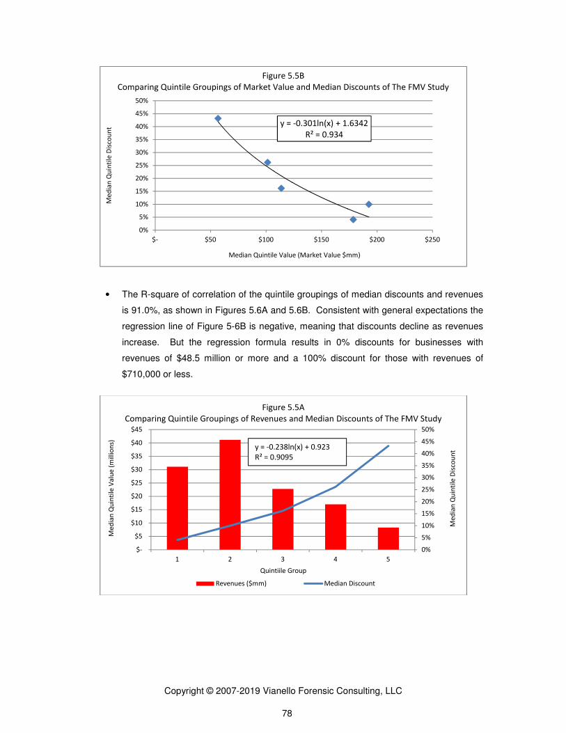
Copyright © 2007-2019 Vianello Forensic Consulting, LLC 78
• The R-square of correlation of the quintile groupings of median discounts and revenues
is 91.0%, as shown in Figures 5.6A and 5.6B. Consistent with general expectations the
regression line of Figure 5-6B is negative, meaning that discounts decline as revenues
increase. But the regression formula results in 0% discounts for businesses with
revenues of $48.5 million or more and a 100% discount for those with revenues of
$710,000 or less.
y = -0.301ln(x) + 1.6342
R² = 0.934
0%
5%
10%
15%
20%
25%
30%
35%
40%
45%
50%
$- $50 $100 $150 $200 $250
Figure 5.5B
Comparing Quintile Groupings of Market Value and Median Discounts of The FMV Study
Me
dia
nQ
uin
tile
Dis
cou
nt
Median Quintile Value (Market Value $mm)
0%
5%
10%
15%
20%
25%
30%
35%
40%
45%
50%
$-
$5
$10
$15
$20
$25
$30
$35
$40
$45
1 2 3 4 5
Revenues ($mm) Median Discount
Figure 5.5A
Comparing Quintile Groupings of Revenues and Median Discounts of The FMV Study
Me
dia
n Q
uin
tile
Va
lue
(m
illio
ns)
Me
dia
nQ
uin
tile
Dis
cou
nt
Quintiile Group
y = -0.238ln(x) + 0.923
R² = 0.9095

Copyright ©
• The R-square of correlation of
assets is 95.6%, as shown in Figures
expectations the regression line of Figure
decline as total assets increase
businesses with total assets of $136 million or more a
total assets of $260,000 or less.
0%
5%
10%
15%
20%
25%
30%
35%
40%
45%
50%
$- $5 $10
Comparing Quintile Groupings of Revenues
Me
dia
n Q
uin
tile
Dis
cou
nt
$-
$20
$40
$60
$80
$100
$120
1
Comparing Quintile Groupings of Total Assets
Me
dia
n Q
uin
tile
Va
lue
(m
illio
ns)
Copyright © 2007-2019 Vianello Forensic Consulting, LLC 79
square of correlation of the quintile groupings of median discounts and total
s 95.6%, as shown in Figures 5.6A and 5.6B. Consistent with general
expectations the regression line of Figure 5.6B is negative, meaning that discounts
decline as total assets increase. But the regression formula results in 0% discount
businesses with total assets of $136 million or more and a 100% discount for those with
total assets of $260,000 or less.
y = -0.238ln(x) + 0.923
R² = 0.9095
$10 $15 $20 $25 $30 $35 $40
Median Quintile Value (Revenues $mm)
Figure 5.5B
Comparing Quintile Groupings of Revenues and Median Discount of The FMV Study
0%
5%
10%
15%
20%
25%
30%
35%
40%
45%
50%
2 3 4 5
Total Assets ($mm) Median Discount
Figure 5.6A
Comparing Quintile Groupings of Total Assets and Median Discount of The FMV Study
y = -0.16ln(x) + 0.7851
R² = 0.9558
Quintiile Group
median discounts and total
B. Consistent with general
B is negative, meaning that discounts
ut the regression formula results in 0% discounts for
nd a 100% discount for those with
$45
FMV Study
10%
15%
20%
25%
30%
35%
40%
45%
50%
FMV Study
Me
dia
nQ
uin
tile
Dis
cou
nt

Copyright © 2007-2019 Vianello Forensic Consulting, LLC 80
• The R-square of correlation of the quintile groupings of median discounts and net book
value is 96.9%, as shown in Figures 5.7A and 5.7B. Consistent with general
expectations the regression line of Figure 5.7B is negative, meaning that discounts
decline as total assets increase. But the regression formula results in 0% discounts for
businesses with net book values of $62 million or more and a 100% discount for those
with total assets of $250,000 or less.
y = -0.16ln(x) + 0.7851
R² = 0.9558
0%
5%
10%
15%
20%
25%
30%
35%
40%
45%
50%
$0 $20 $40 $60 $80 $100 $120
Median Quintile Value (Total Assets $mm)
Figure 5.6B
Comparing Quintile Groupings of Total Assets and Median Discount of The FMV Study
Me
dia
nQ
uin
tile
Dis
cou
nt
0%
5%
10%
15%
20%
25%
30%
35%
40%
45%
50%
$0
$10
$20
$30
$40
$50
$60
1 2 3 4 5
Book Value of Equity ($mm) Median Discount
Figure 5.7A
Me
dia
n Q
uin
tile
Va
lue
(m
illio
ns)
Me
dia
nQ
uin
tile
Dis
cou
nt
Quintiile Group
Comparing Quintile Groupings of Net Book Value and Median Discount of The FMV Study
Me
dia
nQ
uin
tile
Dis
cou
nt
Quintiile Group
y = -0.181ln(x) + 0.7469
R² = 0.9691

Copyright © 2007-2019 Vianello Forensic Consulting, LLC 81
• The R-square of correlation of the quintile groupings of median discounts and market-to-
book ratios is 88.2%, as shown in Figures 5.8A and 5.8B. Consistent with general
expectations the regression line of Figure 5.8B is positive, meaning that discounts
increase as market-to-book ratios increase. But the regression formula results in 0%
discounts for businesses with market-to-book ratios of 2.625x or less and a 100%
discount for those with market-to-book rations of 27x or more.
y = -0.181ln(x) + 0.7469
R² = 0.9691
0%
5%
10%
15%
20%
25%
30%
35%
40%
45%
50%
$- $10 $20 $30 $40 $50 $60
Figure 5.7B
Comparing Quintile Groupings of Net Book Value and Median Discount of The FMV Study
Median Quintile Value (Net Book Value $mm)
Me
dia
nQ
uin
tile
Dis
cou
nt
0%
5%
10%
15%
20%
25%
30%
35%
40%
45%
50%
0
1
2
3
4
5
6
7
1 2 3 4 5
MTB Ratio Median Discount
Figure 5.8A
Comparing Quintile Groupings of Market-to-Book Ratio and Median Discount of The FMV Study
Me
dia
n Q
uin
tile
Va
lue
(m
illio
ns)
Me
dia
nQ
uin
tile
Dis
cou
nt
y = 0.4269ln(x) - 0.4117
R² = 0.8821
Quintiile Group

Copyright © 2007-2019 Vianello Forensic Consulting, LLC 82
• The R-square of correlation of the quintile groupings of median discounts and net
income is a very low 3.65%, as shown in Figures 5.9A and 5.9B. This association
illogically results in higher discounts as net income increases.85
85
The regression formula is linear because negative values cannot be regressed logarithmically.
y = 0.4269ln(x) - 0.4117
R² = 0.8821
0%
5%
10%
15%
20%
25%
30%
35%
40%
45%
50%
0 1 2 3 4 5 6 7
Figure 5.8B
Comparing Quintile Groupings of Market-to-Book Ratio and Median Discount of The FMV Study
Me
dia
nQ
uin
tile
Dis
cou
nt
Median Quintile Value (MTB Ratio x:1)
0%
5%
10%
15%
20%
25%
30%
35%
40%
45%
50%
-$5
-$5
-$4
-$4
-$3
-$3
-$2
-$2
-$1
-$1
$0
1 2 3 4 5
Net Income ($mm) Median Discount
Figure 5.9A
Comparing Quintile Groupings of Net Income and Median Discount of The FMV Study
Me
dia
n Q
uin
tile
Va
lue
(m
illio
ns)
Me
dia
nQ
uin
tile
Dis
cou
nt
y = 0.0258x + 0.2839
R² = 0.0365
Quintiile Group

Copyright © 2007-2019 Vianello Forensic Consulting, LLC 83
• The R-square of correlation the quintile groupings of median discounts and net profit
margins is 92.1%, as shown in Figures 5.10A and 5.10B. Consistent with general
expectations the regression line of Figure 5.10B is negative, meaning that discounts
decline as net profit margins increase. But the regression formula results in 0%
discounts for businesses with net profit margins of 3.725% or more and 100% discounts
for those with net profit margins of -96% or less.
y = 0.0258x + 0.2839
R² = 0.0365
0%
5%
10%
15%
20%
25%
30%
35%
40%
45%
50%
-$5 -$4 -$3 -$2 -$1 $0
Me
dia
nQ
uin
tile
Dis
cou
nt
Figure 5.9B
Comparing Quintile Groupings of Net Income and Median Discount of The FMV Study
Median Quintile Value (Net Income $mm)
0%
5%
10%
15%
20%
25%
30%
35%
40%
45%
50%
-45%
-40%
-35%
-30%
-25%
-20%
-15%
-10%
-5%
0%
1 2 3 4 5
Net Profit Margin Median Discount
Figure 5.10A
Comparing Quintile Groupings of Net Profit Margin and Median Discount of The FMV Study
Me
dia
n Q
uin
tile
Va
lue
(%
ma
rgin
)
Me
dia
nQ
uin
tile
Dis
cou
nt
Quintiile Group
y = -1.0074x + 0.0376
R² = 0.9206

Copyright © 2007-2019 Vianello Forensic Consulting, LLC 84
• The R-square of correlation of the quintile groupings of median discounts and price
volatility is 98.3%, as shown in Figures 5.11A and 5.11B. Consistent with general
expectations the regression line of Figure 5.11B is positive, meaning that discounts
increase as volatility increases. But the regression formula results in 0% discounts for
businesses with price volatility of 59% or less and 100% discounts for those with price
volatility of 215% or more.
y = -1.0074x + 0.0376
R² = 0.9206
0%
5%
10%
15%
20%
25%
30%
35%
40%
45%
50%
-45% -40% -35% -30% -25% -20% -15% -10% -5% 0%
Figure 5.10B
Comparing Quintile Groupings of Net Profit Margin and Median Discount of The FMV Study
Median Quintile Value (% Profit Margin)
Me
dia
nQ
uin
tile
Dis
cou
nt
0%
5%
10%
15%
20%
25%
30%
35%
40%
45%
50%
0%
20%
40%
60%
80%
100%
120%
1 2 3 4 5
Volatility Median Discount
Figure 5.11A
Comparing Quintile Groupings of Volatility and Median Discount of The FMV Study
Me
dia
n Q
uin
tile
Va
lue
(%
vo
lati
lity)
Me
dia
nQ
uin
tile
Dis
cou
nt
Quintiile Group
y = 0.7752ln(x) + 0.4111
R² = 0.9834

Copyright © 2007-2019 Vianello Forensic Consulting, LLC 85
• The R-square of correlation of the quintile groupings of median discounts and the
volatility index (VIX) is 71.0%, as shown in Figures 5.12A and 5.12B. Consistent with
general expectations the regression line of Figure 5.12B is positive, meaning that
discounts increase as volatility increases. But the regression formula results in 0%
discounts when the VIX is 16.25 or less and 100% discounts when it is 30.5 or more.
y = 0.7752ln(x) + 0.4111
R² = 0.9834
0%
5%
10%
15%
20%
25%
30%
35%
40%
45%
50%
0% 20% 40% 60% 80% 100% 120%
Figure 5.11B
Comparing Quintile Groupings of Price Volatility and Median Discount of The FMV Study
Me
dia
nQ
uin
tile
Dis
cou
nt
Median Quintile Value (% Price Volatility)
0%
5%
10%
15%
20%
25%
30%
35%
40%
45%
50%
0
5
10
15
20
25
1 2 3 4 5
VIX Median Discount
Figure 5.12A
Comparing Quintile Groupings of VIX and Median Discount of The FMV Study
Me
dia
n Q
uin
tile
Va
lue
(in
de
x)
Me
dia
nQ
uin
tile
Dis
cou
nt
Quintiile Group

Copyright © 2007-2019 Vianello Forensic Consulting, LLC 86
Table 5.5 summarizes the regression formula results described above. Although it can
be questioned whether grouped data such as quintiles are statistically valid, it is clear that the Net
Income variable is contradictory to DLOM (discounts go up as net income goes up), while the Net
Profit Margin parameter is highly suspect (no discount if profit margin is greater than 3.725%).
For the remaining variables practitioners should consider whether the ranges of implied discounts
are reasonable.
Table 5.5
Range of Discounts Implied from Financial Characteristics
of Transactions in the Stout Study
Discount Range
Independent Variable 0% Discount 100% Discount
Market Value $227,500,000 $830,000
Revenues $48,500,000 $710,000
Total Assets $136,000,000 $260,000
Net Book Value $62,000,000 $250,000
Market-to-Book Ratio 2.625x 27x
Net Income ($11,000,000) $27,600,000
Net Profit Margin 3.725% -96.00%
12-Month Price Volatility 59% 215%
Volatility Index (VIX) 30.50 16.25
y = 1.5798ln(x) - 4.4041
R² = 0.7104
0%
5%
10%
15%
20%
25%
30%
35%
40%
45%
50%
0 5 10 15 20 25
Figure 5.12B
Comparing Quintile Groupings of VIX and Median Discount of The FMV Study
Me
dia
nQ
uin
tile
Dis
cou
nt
Median Quintile Value (VIX)

Copyright © 2007-2019 Vianello Forensic Consulting, LLC 87
Section 3 — The Discounts Reported in the Stout Restricted Stock Study Are Consistent with Past Changes in SEC Rule 144 Required Holding Periods It was pointed out in Chapter 4 that the discounts reported in the Pluris
® database are not
intuitively consistent with changes in SEC Rule 144 required holding periods; average discounts
should decrease as required holding periods decrease. However, the discounts reported in The
Stout Study are intuitively consistent:
• The discounts for transactions reported with 2-year holding periods average 22.47%
(24.1% if zero and negative discounts are excluded);
• The discounts for transactions reported with 1-year holding periods average 19.1%
(21.9% if zero and negative discounts are excluded); and
• The discounts for transactions reported with 6-month holding periods average 14.3%
(15.9% if zero and negative discounts are excluded).
Section 4 — How the Stout Restricted Stock Study Discounts Correlate with the Other Metrics Reported in the Database A more robust analysis occurs if the detailed data reported in The Stout Study is
analyzed without the quintile grouping approach employed by Stout Table 5.6 reports the results
of linear and logarithmic regressions of the principal independent variables reported for the 769
transactions in The Stout Study. The strongest statistical relationship with restricted stock
discounts is shown by annual price volatility. That relationship has R-squares of correlation of
10.6% and 15.4% based on the linear and logarithmic regressions, respectively.86
It makes
sense that negotiated restricted stock discounts are affected logarithmically by changes in price
volatility. In other words, the changes in discounts and price volatility are not likely to represent a
straight line.
86
Price per share shows the next strongest relationship with a 13.1% logarithmic R-square of correlation. Intuition does not explain why share price would affect the discount. The next highest logarithmic R-squares of correlation are shown by the total liabilities, gross placement amount, and market value variables. It makes intuitive sense that discounts would vary with these variables because they have risk implications not present with price per share.

Copyright © 2007-2019 Vianello Forensic Consulting, LLC 88
Table 5.6
Summary of Detailed Regression Analyses of The Stout Study
Number of
Transactions
Linear Logarithmic
R-Square R-Square Slope
Block Size 769 0.02230 0.31320 0.00440
Book Value 769 0.01440 0.00000 negatives
Dividend Yield none none none none
EBIT 733 0.00140 0.00000 negatives
EBIT Margin 681 0.00740 -0.00030 negatives
EBITDA 733 0.00170 0.00000 negatives
Gross Placement Amount 769 0.01210 0.00000 0.08250
Market Value 769 0.01680 0.00000 0.07550
MTB Ratio 769 0.03030 -0.00003 negatives
Net Income from Continuing Operations 769 0.00020 0.00000 negatives
Net Profit Margin 717 0.00700 -0.00020 negatives
Pretax Income 769 0.00040 0.00000 negatives
Price per Share 769 0.03830 -0.00270 0.13100
Prior Year Dividends per Share 769 0.01580 -0.06440 zeros
Retained Earnings 768 0.01240 0.00000 negatives
Shares Outstanding 769 0.00920 0.00000 0.02110
Shares Placed 769 0.00007 0.00000 0.00280
Shares Placed to Volume 769 0.01260 0.00009 zeros
Total Assets 769 0.00650 0.00000 zeros
Total Current Assets 716 0.00140 0.00000 zeros
Total Current Liabilities 717 0.00120 0.00000 zeros
Total Interest Bearing Debt 768 0.00370 0.00000 zeros
Total Liabilities 222 0.00740 0.00000 0.08710
Total Revenues 769 0.00450 0.00000 zeros
Transaction Day Close 769 0.00170 -0.00050 0.01420
VIX 695 0.00100 0.00080 0.00210
VIX 1Month 699 0.00090 0.00080 0.00190
VIX 3Month 696 0.00130 0.00090 0.00240
Volatility 740 0.10630 0.06040 0.15350
Volume 769 0.00050 0.00000 zeros
Volume to Shares Outstanding 769 0.01810 0.06150 zeros
Z Score 632 0.00610 0.00001 negatives
The Stout DLOM calculator relies on seven variables to benchmark DLOM: market value
of equity, total revenues, total assets, shareholders’ equity (“book value”), market-to-book ratio,
net profit margin, and 12-month price volatility. Of the 769 transactions comprising The Stout
Study, 217 had positive values for all seven of the variables used by the Stout calculator. Table
5.7 summarizes certain statistical characteristics of the 217 transactions according each of the
seven calculator variables. Additionally, Table 5.7 presents the results of linear regressions of

Copyright © 2007-2019 Vianello Forensic Consulting, LLC 89
the transaction issuers’ financial characteristics (i.e., the variables) and the corresponding
transaction discounts. All of the variables showed logical relationships with discounts.
Table 5.7
Statistical Attributes of 217 Stout Restricted Stock Transactions with Positive Discounts and Positive Financial Parameters
Transaction Discount
Market Value
Total Revenues
Total Assets
Book Value
MTB Ratio
Net Profit Margin Volatility
Average ($000) 18.2% $255,014 $239,082 $814,147 $123,713 5.6 12.5% 67.0%
Std Dev ($000) 15.1% $622,326 $1,281,950 $3,081,418 $359,788 12.4 37.6% 43.7%
Coefficient of Variation 0.8 2.4 5.4 3.8 2.9 2.2 3.0 0.7
Count 217 217 217 217 217 217 217 217
Standard Error ($000) 1.0% $42,246 $87,024 $209,180 $24,424 0.8 2.5% 3.0%
95% Confidence Interval
• High ($000) 20.2% $337,816 $409,650 $1,224,141 $171,585 7.3 17.5% 72.8%
• Low ($000) 16.2% $172,211 $68,514 $404,154 $75,842 4.0 7.5% 61.2%
R-square of Linear Correlation with Discounts N/A 1.81% 1.02% 0.90% 2.32% 4.25% 0.62% 22.92%
Direction of Slope N/A Negative Negative Negative Negative Positive Negative Positive
Slope logic N/A Logical Logical Logical Logical Logical Logical Logical
The 217 transactions comprising Table 5.7 were tested for statistical significance. Price
volatility and market-to-book ratio have the highest linear R-squares of correlation with
transaction discounts at 22.92% and 4.25%, respectively. Regression analysis of the group of
transactions shows an overall 27.6% R-square of correlation. But Table 5.8 shows that only
market-to-book ratio and price volatility are statistically significant with t-Stats greater than 2.0
and P-values less than 5%. Price volatility shows much more statistical strength than market-to-
book ratio. Removing price volatility from the group reduced the R-square of correlation to 8.0%,
with market-to-book value remaining the only statistically significant variable. The raw data for
market value, total revenues, total assets book value, and net profit margin does not appear to
offer a statistical basis for benchmarking DLOM.

Copyright © 2007-2019 Vianello Forensic Consulting, LLC 90
Table 5.8 Multivariate Regression Analysis of 217 Stout Restricted Stock
Transactions with Discounts and Financial Parameters Greater than Zero
Valuation Variable t Stat P-value Significant?
Market Value 0.20904 0.83461 No
Total Revenues -0.28434 0.77642 No
Total Assets 1.64831 0.10079 No
Book Value -1.42682 0.15512 No
Market-to-Book Ratio 2.48965 0.01356 Yes
Net Profit Margin -1.02218 0.30787 No
Price Volatility 7.53149 1.485E-12 Yes
The above analyses allow one to conclude with reasonable certainty that negotiators
consider the issuer’s stock price volatility when negotiating restricted stock discounts. Therefore,
a reliable method for estimating discounts should focus on stock price volatility. Of course, it is
unknown how negotiators estimate stock price volatility. It may be based on 12-month historical
periods as analyzed here, other historical time periods, trends, or otherwise. But since investing
is a matter of future expectations, it is reasonable to assume that negotiators of restricted stock
prices are interested in the price risks associated with an expected holding period for their
investment. It seems clear however that DLOM conclusions should be based primarily on
estimated price risk over a period of illiquidity.
The Stout Study provides two data fields that are helpful in further analyzing the
correlation of price volatility and discounts. Those are the Rule 144 holding period and the
registration rights applicable to the restricted stock transaction. The Rule 144 information allows
better consideration of the relationship of discounts to both time and price volatility. The
registration rights information allows better consideration of the relationship of discounts to risk
and liquidity. Table 5.9 summarizes the results of logarithmic regressions of price volatility versus
different combinations of the time and liquidity-based information. Whereas the R-square of
correlation for all 679 transactions was 21.1%, significant improvement was found in the
correlation of the price volatility and the discounts for restricted stock transactions without
registration rights and subject to a six-month Rule 144 holding period requirement. Those
conditions applied to 24 restricted stock transactions that show a 35.0% R-square of correlation
with the reported discounts. This result suggests that the discount negotiators were influenced to
some extent by some combination of the period of illiquidity and registration rights.

Copyright © 2007-2019 Vianello Forensic Consulting, LLC 91
Table 5.9
R-Squares of Logarithmic Correlation for Restricted Stock Transactions
in the Stout Study with Both Positive Discounts and Price Volatility Reported
Rule 144 Holding Period
All 2 Years 1 Year 6 Months
Rule 144 Holding Period
R-square 21.1% 20.5% 22.8% 26.9%
Number of Transactions 679 232 318 129
With Registration Rights
R-square 15.4% 15.8% 14.2% 23.1%
Number of Transactions 309 43 162 104
Without Registration Rights
R-square 19.3% 21.7% 17.9% 35.0%
Number of Transactions 233 184 25 24
Unknown Registration Rights
R-square 24.2% 22.9% 24.1% N/A
Number of Transactions 137 5 131 1
Section 5 — The Stout DLOM Methodology
The Stout DLOM methodology is generally similar the Pluris® DLOM methodology, but
with two principal differences. First, Stout bases its median values on a quintile division of its
database transactions, while Pluris® bases its median values on a quartile division of its database
transactions. Stout’s® use of quintiles instead of quartiles provides its method a slight
methodological advantage. Second, the variables used to benchmark valuation subjects are
somewhat different. Both benchmark on total assets, total revenues, book equity, net profit
margin, and market-to-book value ratio. The Stout method also benchmarks on market value of
equity and price volatility, while the Pluris® method benchmarks on EBITDA, net income, and
enterprise value. Stout’s® use of price volatility as a benchmarking variable provides it with a
statistically significant metric that the Pluris® method does not employ (except as a user-defined
variable).
Stout states that it “typically does not consider industry classification to be a significant
determinant of DLOM.”87
Nor does the Pluris® DLOM calculator employ industry as a benchmark.
87
“Determining Discounts for Lack of Marketability – A companion Guide to The RMV Restrict Stock Study,” FMV Opinions, Inc., 2015, page 22.

Copyright © 2007-2019 Vianello Forensic Consulting, LLC 92
These omissions may be due to the dearth of transactions in specific SIC codes. But the average
discounts of the Stout restricted stock transactions vary greatly by industry as Figure 5.13 shows.
It is therefore illogical to exclude industry as a benchmarking variable.
The initial goal of the Stout DLOM methodology is to determine a restricted stock
equivalent discount (“RSED”).88
There are five steps to this methodology:
1. The Stout database is sorted into five equal percentile groups (quintiles) for each
variable and the median discount is computed for each group.89
2. The valuation subject’s financial risk parameters are compared to the quintile group
parameters to determine in which quintile segment the subject’s parameter falls.90
3. The financial risk parameters of the valuation subject is “matched” to the quintile
groups to obtain median discounts from the quintile segment deemed to be
applicable to the subject company. The obtained median discounts are then
averaged, with greater weight being given to quintile subsamples that have the
greatest number of transactions.91
The resulting average is considered to be the
RSED.92
88
Id., at page 23. 89
Id. 90
Id. 91
Id. Stout states that the weights are based on which factors tend to be the most important determinants of DLOM. Stout considers that the “key” variables are market value, total assets, shareholders’ equity, and price volatility.91
0%
5%
10%
15%
20%
25%
30%
0-9
99
10
00
-19
99
20
00
-29
99
30
00
-39
99
40
00
-49
00
50
00
-59
99
60
00
-69
99
70
00
-79
99
80
00
-87
42
Standard Industrial Classification Code Range
Ave
rag
e D
isco
un
t
Figure 5.13
Average Restricted Stock Discount by one-Digit SIC Code

Copyright © 2007-2019 Vianello Forensic Consulting, LLC 93
4. The Stout methodology may then employ a “market volatility adjustment” to yield an
adjusted RSED (“ARSED”) in the event that a valuation date occurs within a period of
abnormally high market volatility. Stout states that transactions that occurred in
periods of high market volatility tend to exhibit higher discounts.93
Stout states that
the RSED tends to underestimate the actual transaction discounts for high-VIX
transactions.94
Accordingly, Stout employs the “market volatility adjustment” for all
one-year SEC Rule 144 holding period data high-VIX transactions.95
This results in
multiplicative adjustments of 1.16:1 for transactions in the 60th to 80
th VIX percentile
group and of 1.23:1 for transactions in the 80th to 100
th VIX percentile group.
96 Stout
uses implied adjustment factors for VIX index values greater than 32.9.97
The VIX
statistic utilized for this analysis is the trailing six-month average VIX as of the
transaction date.98
Stout advises that appraisers should also consider the possibility
that a downward adjustment to the RSED may be appropriate during times of
historically low stock market volatility.99
5. According to Stout, the ARSED represents the discount appropriate for a public
company issuing restricted stock that will ultimately have access to a public trading
market, and that an incremental private equity discount (“PED”) (generally a positive
discount, but sometimes a negative discount) is needed to determine the discount
appropriate for a privately held business.100
The PED increment is derived by
comparing the discount indications for large-block transactions with those for small-
block transactions.101
Stout states:
92
Id., at page 24. 93
Id. 94
Id. 95
Id. 96
Id. 97
Id. 98
Id. 99
Id. 100
Id. at page 25. 101
Id.

Copyright © 2007-2019 Vianello Forensic Consulting, LLC 94
[Key Point] Unlike differing percentage minority interest in public companies, which have differing degrees of liquidity…,differing percentage minority interest in private entities generally have similar degrees of liquidity. Furthermore, the degree of liquidity of typical minority interests in private companies is most similar to the degree of liquidity of large blocks or restricted stock in public companies.
102
Stout provides no substantiation for this statement, which is an essential
foundation for its PED methodology. To the contrary, regression analysis of block
size and transaction discounts as reported in The Stout Study yields extremely low R-
squares of correlation. See Table 5.6.
According to Stout, large block transactions most closely resemble private equity
and small-block transactions most resemble RSED.103
As discussed in Chapter 4,
these supposed similarities are questionable. Large stock blocks in privately held
companies often represent controlling interests, which are generally considered to be
more liquid and to require lower discounts than non-controlling interests. Why are
large blocks of restricted stock not similarly more liquid than the smaller blocks? It
seems illogical that smaller-block non-controlling interests would require smaller
discounts than the larger-blocks that potentially represent some degree of control of
the enterprise.
Setting aside what may be a seriously flawed PED methodology, it is reasonable that the
liquidity discount applicable to an interest in a privately held business should be greater than its
RSED. Some amount of PED is likely appropriate when valuing a privately held business.
Section 6 — Testing the Stout DLOM Methodology
The reliability of the Stout DLOM methodology is easily tested by (1) dividing into
quintiles the seven Stout DLOM parameters (i.e., market value of equity, total revenues, total
assets, shareholders’ equity, market-to-book ratio, net profit margin, and 12-month price
volatility); (2) determining the median discount for each quintile segment of each parameter; (3)
matching the equivalent characteristics of the restricted stock issuers to the appropriate quintile
segment; (4) averaging the resulting median discounts; and (5) comparing the DLOM results with
the transactions discounts using linear regression.104
Ideally the relationship is one-to-one. The
102
Id. 103
Id. 104
It is not necessary to weight the discounts for this exercise because the financial characteristics of the actual issuers should directly correspond to their negotiated discounts. Likewise, it is not necessary to adjust the resulting DLOM for market volatility conditions because

Copyright © 2007-2019 Vianello Forensic Consulting, LLC 95
average ideally also would closely approximate the restricted stock discount of the issuer or, at
least, for the population of transactions as a whole.
Figure 5.14 shows that the distribution of the quintile DLOMs is not consistent with the
reported discounts of 638 underlying transactions with discounts greater than zero. While the
distribution of discounts extends from less than 1% to 92%, the distribution of quintile DLOMs is
bookended within the range of 11% to 27%. On a prima facie basis the quintile approach does
not emulate the restricted stock discounts and is not a reliable way to estimate DLOMs.
Table 5.10 shows different groups of restricted stock transactions extracted from The
Stout Study. The transactions selected for analysis are those 638 for which The Stout Study
reports positive discounts and values for each of the seven Stout DLOM calculator parameters
(i.e., market value of equity; total revenues; total assets; shareholders’ equity; market-to-book
ratio; net profit margin; and 12-month price volatility). The groups are further differentiated by the
Rule 144 time period and registration rights characteristics stated in the Study, and are ranked in
descending order according to the number of transactions comprising each group.
the discounts were negotiated contemporaneously with the prevailing conditions. Finally, a PED is unnecessary for this exercise since the issuers are public companies.
0
10
20
30
40
50
60
70
80
0 5 10 15 20 25 30 35 40 45 50 55 60 65 70 75 80 85 90 95 100
Transaction Discounts Quintile DLOMs
Nu
mb
er
of
Occ
urr
en
ces
Percentage Discount or DLOM
Figure 5.14
Distribution Comparison of the Discounts and Quintile DLOMs for
638 FMV Resricted Stock Transactions with Positive Discounts

Copyright © 2007-2019 Vianello Forensic Consulting, LLC 96
Table 5.10
Correlation of Median Quintile DLOMs with Positive Discount Transactions
Rule 144 Time Period
Registration Rights
Transaction Count
Average Transaction
Discount
Average Stout
DLOM Regression Line Slope
Y-Axis Intercept R-Square
All All 638 21% 18% 1.926 -13.5% 26%
2 Years No 178 24% 22% 1.714 -14.1% 29%
1 Year Yes 159 17% 14% 2.420 -16.5% 30%
1 Year Blank 121 27% 22% 2.067 -18.3% 25%
6 Months Yes 94 15% 12% 4.230 -34.3% 15%
2 Years Yes 40 24% 24% 3.391 -56.0% 45%
1 Year No 23 25% 23% 1.436 -7.9% 22%
6 Months No 18 17% 17% 2.155 -19.5% 60%
2 Years Blank 5 23% 23% 1.000 0.0% 100%
A perfect linear regression has an x coefficient of 1.0, a y intercept of 0.0%, and an R-
square of correlation of 100%. That result occurred with the five-transaction group with a two-
year Rule 144 holding period and unknown registration rights. But this is merely a proof of the
regression methodology, because a five-transaction group divided into quintiles should result in a
perfect correlation as each DLOM equals its corresponding discount. Table 5.10 shows that none
of the other transaction groups provides a reasonable corroboration of DLOMs with the actual
discounts. For example, the best of the other correlations is the 18-transaction group with a six-
month Rule 144 holding period and no registration rights. This group has a 60% R-square of
correlation of DLOMs to discounts, and the average DLOM equals the average discount—17%.
Those values are deceptive, however, because the x coefficient slope is 2.155-to-1 and the y
intercept is -19.5%. Figure 5.15 demonstrates why this group does not offer a satisfactory
justification of the Stout methodology despite its relatively high R-square of correlation. DLOMs
based on this quintile group would always be greater than 19% but less than 56% despite that the
transactions on which they are benchmarked may have discounts ranging from 0% to 100%.
[Intentionally blank.]

Copyright © 2007-2019 Vianello Forensic Consulting, LLC 97
None of the other groupings reported in Table 5.10 offers a corroboration of DLOMs
using the underlying restricted stock transactions. All have lower R-squares of correlation and
unsatisfactory x coefficients and y intercepts.
y = 2.1552x - 19.45
R² = 0.5956
-60
-40
-20
0
20
40
60
80
100
-20 0 20 40 60 80 100Pe
rce
nta
ge
Dis
cou
nt
Percentage FMV DLOM
Figure 5.15
Correlation of DLOMs to Discounts for 18-Transaction Group

Copyright © 2007-2019 Vianello Forensic Consulting, LLC 98
Chapter 6
THE PRICE AND TIME VARIABLES THAT UNDERLIE DLOM
The business valuation concept of marketability deals with the liquidity of the ownership
interest.105
The ease and certainty with which an investor can quickly convert an investment to
cash represent two very different variables. Ease of sale is a function of how quickly a sale can
occur—the period of time it will take the seller to liquidate an investment. This period of time can
vary greatly depending on the manner of sale. For example, liquidation sales can occur quickly
and generally occur at lower prices, while orderly sales usually take longer to explore the
marketplace of reasonable buyers and generally secure greater than liquidation prices. The time
periods for private sales and public offerings also differ. In every instance, however, the “quickly”
variable commences with a decision by the seller to initiate the sale process.
Price risk represents a lack of certainty that the expected price will be realized in an
eventual sale. Price volatility is a way of quantifying the impact of the “certainty” variable during
the period of time that it is being offered for sale. If market prices for similar investments fall
dramatically while the marketplace is being explored, then the seller will have lost the opportunity
to lock in the higher price that existed at the time the sell decision was made. Conversely, if the
sale price is fixed for some reason (e.g., a listing agreement or a call price) and market prices for
similar investments rise dramatically during the marketing period, the seller will have lost the
opportunity to realize the increased value.
The time and price risk variables work together when determining an appropriate DLOM.
Relative to immediately marketable investments, the value of illiquid investments must be
discounted to reflect the uncertainties of the timing and realizable price of a sale. For example,
assets may be subject to greater illiquidity during periods of market stress that would call for an
increased DLOM. Transaction costs (particularly if similar costs are inherited by the buyer) may
also impact the DLOM. These uncertainties reflected in business valuations are what DLOM
should represent.
Logically, the economic costs of time and price uncertainties can be reduced to the price
risk faced by an investor during the particular period of time that an illiquid investment is being
offered for sale. In the market for publicly traded stocks, the volatility of stock prices represents
risk. Investments with no price volatility have no DLOM, because they can be arbitraged to
negate the risk of a period of restricted marketing—although perhaps with an interest cost.
Conversely, volatile investments that are immediately marketable can be sold at the current price
to avoid the risk of future volatility. It is different for investments in privately-held businesses.
105
Shannon P. Pratt and Alina V. Niculita, Valuing a Business, 5th Edition: The Analysis and
Appraisal of Closely Held Companies. (McGraw-Hill, 2007), page 417.

Copyright © 2007-2019 Vianello Forensic Consulting, LLC 99
The marketing period illiquidity experienced by the seller of a non-publicly traded business
interest brings with it an economic cost reflective of the risk associated with the inability to realize
gains and to avoid losses during that time period.106
The longer that time period, the more the
value of the business is exposed to adverse events in the marketplace and in the operations of
the business, and the greater the DLOM that is required to equate the investment to an
immediately liquid counterpart. Some or all of the economic cost associated with a period of
illiquidity can be estimated using option pricing formulas such as Black-Scholes or the look-back
formula developed by Francis A. Longstaff, Ph.D. in 2002,107
which relies on estimates of price
volatility (i.e., the certainty variable) and marketing time (i.e., the quickly variable).
Section 1 – Marketing Periods of Private Businesses Transactions
The marketing period for the private sale of a controlling interest in a business is seldom
less than a few months, and can be much longer for a minority position in the business, as the
following events occur:
• Drafting selling documents
• Developing a marketing strategy
• Implementing the marketing strategy
• Screening buyers
• Conducting site visits
• Assisting buyers in their analysis of the company and the interest being sold
• Drafting letters of intent
• Negotiating with the serious buyers
• Assisting buyers with due diligence
• Drafting the contract of sale
• Participating in arranging financing
• Actually closing the deal
The time periods of private sales of businesses were analyzed using 7,960 transactions
from BV Resource's DealStats® database and 10,381 transactions from ValuSource's
BIZCOMPS® database.
108 The DealStats
® database included 32 transactions with zero or
negative marketing periods (the dates may be transposed). Those transactions were excluded
from the analyses below, leaving 7,928 DealStats® transactions for analysis. The population of
106
Id. 107
Francis A. Longstaff, “How Much Can Marketability Affect Security Values?”, The Journal of Finance, Volume I, No. 5, December 1995. 108
Jack R. Sanders, CBA, CBI, CMEA, CVA is the collector and author of the BIZCOMPS®
database.

Copyright © 2007-2019 Vianello Forensic Consulting, LLC 100
the DealStats® transactions occurred from February 1992 through the end of 2011; the population
of the BIZCOMPS® transactions occurred from March 1995 through the end of 2011.
109 For each
transaction, these databases report an associated SIC code; sale initiation date; sale closing
date; and asking price. Each DealStats® transaction also listed a market value of invested capital
(“MVIC”). The two sets of transactions are heavily weighted to 1998 and later years. Figure 6.1
shows the distribution by year of the 7,928 DealStats® and 10,381 BIZCOMPS
® transactions.
Readers will note the substantial declines in listings that occurred in years 2008 and
2009. These were the years of the “Great Recession,” which likely explains the declines.
The average time that elapsed from the initial offering date to the closing date of these
transactions is 211 days for the DealStats® transactions and 214 days for the BIZCOMPS
®
transactions. The standard deviation of the reported time periods is 208 days for the DealStats®
transactions and 176 days for the BIZCOMPS®
transactions.
Figure 6.2 shows the distribution of marketing periods of the population of DealStats®
sales in 30-day increments.110
The peak of the graph is 972 sale transactions that occurred from
109
The transactions reported in the DealStats® and BIZCOMPS
® databases reflect significant
time period lags that can distort contemporaneous time period analysis by favoring sales that occurred quickly. Sales initiated after December 31, 2009, were excluded from both databases to avoid skewing the analyses herein with only short period sales in the years after 2009. Obviously, years have passed since the 2011 cutoff of the transactional data presented herein. The additional transactions subsequently reported in the DealStats
® and BIZCOMPS
® databases
can be expected to have some effect on the results being discussed, and will be analyzed in later updates of this research 110
Sixty-one transactions with marketing periods greater than 1,080 days were aggregated for presentation purposes.
1 2 9 20
1 3 16 23 51
0
200
400
600
800
1,000
1,200
1,400
19
91
19
92
19
93
19
94
19
95
19
96
19
97
19
98
19
99
20
00
20
01
20
02
20
03
20
04
20
05
20
06
20
07
20
08
20
09
Pratt's Stats BIZCOMPS
Figure 6.1
Listing Year Distribution of 7,928 DealStats and 10,381 BIZCOMPS Transactions

Copyright © 2007-2019 Vianello Forensic Consulting, LLC 101
61 to 90 days after being listed for sale. The 972 sales represent 12.3% of the population. One
standard deviation to the right of the mean encompasses marketing periods up to 420 days,
which is 88.5% of the population.
Figure 6.3 shows the distribution of marketing periods of the population of BIZCOMPS®
transactions in 30-day increments.111
The peak of the graph is 1,161 sale transactions that
occurred from 61 to 90 days to sell. The 1,161 sales represent 11.2% of the database. One
standard deviation to the right of the mean encompasses marketing periods of up to 390 days,
which is 88.5% of the population. The transactions reported by BIZCOMPS® occurred faster on
average than those reported in by DealStats®.
111
Ninety-four transactions with marketing periods greater than 990 days were aggregated for presentation purposes.
972
61
0
200
400
600
800
1000
1200
30 120 210 300 390 480 570 660 750 840 930 1020 >1080
Figure 6.2
Distribution of Selling Time of 7,928 DealStats Transactions
Nu
mb
er
of
Clo
sed
Tra
nsa
ctio
ns

Copyright © 2007-2019 Vianello Forensic Consulting, LLC 102
Section 1.A Industry Variations in Selling Time
Separating the DealStats® and BIZCOMPS
® transactions into broad industry groupings
represented by ten two-digit SIC code divisions shows significant variation of selling periods
between industries. See Figure 6.4.
Table 6.1 presents the number of transactions, average selling time in days, and
standard deviation of the selling times by two-digit SIC code. The spread between the fastest
average selling and slowest average selling industry groups is 76 days in the DealStats®
database and 60 days in the BIZCOMPS® database.
1,161
94
-
200
400
600
800
1,000
1,200
1,400
30 120 210 300 390 480 570 660 750 840 930 >990
Figure 6.3
Distribution of Selling Time of 10,381 BIZCOMPS Transactions
Nu
mb
er
of
Clo
sed
Tra
nsa
ctio
ns
-
50
100
150
200
250
300
01-09 10-14 15-17 20-39 40-49 50-51 52-59 60-67 70-89 91-99
Pratt's Stats
BIZCOMPS
Figure 6.4
Average Selling Time by SIC Code
Two Digit SIC Code
Ave
rag
e D
ays
to
Se
ll

Copyright © 2007-2019 Vianello Forensic Consulting, LLC 103
Table 6.1
Selling Time of Private Company Sales by Two-Digit Industry Classification
DealStats® BIZCOMPS
®
SIC Code Range SIC Group
Number of Sale
Transactions
Average Selling Time
in Days Standard Deviation
Number of Sale
Transactions
Average Selling Time
in Days Standard Deviation
01-09 Agriculture, forestry, and fishing 235 199 201 310
218 182
10-14 Mining 9 172 127 - n/a -
15-17 Construction 375 248 260 503 264 198
20-39 Manufacturing 918 226 212 1,060 238 197
40-49 Transportation, communications, electric, gas, and sanitary services 245 220 225 330 204 172
50-51 Wholesale trade 502 231 241 579 232 205
52-59 Retail trade 2,833 208 204 4,053 205 166
60-67 Finance, insurance, and real estate 136 236 249 217 208 193
70-89 Services 2,673 200 193 3,329 207 168
91-99 Public administration 2 246 257 none n/a -
All industries 7,928 211 208 10,381 214 176
The construction industry group had the longest average marketing period in both the
DealStats® and BIZCOMPS
® databases: 248 days and 264 days, respectively. The
finance/insurance/real estate and manufacturing industry groups also had marketing periods
longer than the mean in both databases.112
Businesses reported in the mining industry sold relatively quickly in an average of 172
days, but is based on only nine translations in the DealStats® database. The BIZCOMPS
®
database contains no mining industry transactions. The retail and services industry groups also
had marketing periods shorter than the mean in both databases. The DealStats® and
BIZCOMPS® databases had inconsistent results relative to the mean for the
agriculture/forestry/fishing, transportation/communications/electric/gas/sanitary services, and
finance/insurance/real estate industry groups.
The above results show that average marketing periods are materially different for
businesses operating in different industries. The widely varying standard deviations of marketing
periods add to the differences that can be expected when comparing one business to another.
112
The public administration industry group is ignored since it represents the sale of just two businesses.

Copyright © 2007-2019 Vianello Forensic Consulting, LLC 104
Section 1.B Selling Time from Year-to-Year
Figure 6.5 shows the average selling time of the DealStats® and BIZCOMPS
®
transactions when they are divided according to the year in which the businesses were listed for
sale. When considering Figure 6.5, keep in mind that the two databases have very few
transactions prior to 1998, which may affect the averages in those years. See Figure 6.1. Figure
6.5 shows a reduction in average selling times in 2008 and 2009, the years of the “Great
Recession.” DealStats® transactions with listing dates in 2007 took an average 228 days to sell,
but those listed in 2008 and 2009 took, respectively, 214 and 204 days on average to sell.
BIZCOMPS® transactions with listing dates in 2007 took an average 237 days to sell, but those
listed in 2008 and 2009 took, respectively, 181 and 202 days on average to sell. These results,
seemingly contrary to “Great Recession” intuition, may be an indication that the businesses listed
for sale in 2008 and 2009 were sold under duress, were more desirable than historically because
fewer troubled business may have been offered for sale, or may be a reflection of reduced
supply. The private sale databases do not lend themselves to a ready determination of the cause
of the shortened selling periods.
Section 1.C The Effect of Asking Price on Selling Times
The DealStats® and BIZCOMPS
® databases provide the asking prices for most of the
reported transactions. However, 565 DealStats® transactions and one BIZCOMPS
® transaction
have no asking price reported. These transactions were excluded from the asking price analysis.
The range of asking prices of the resulting transaction populations were from $3,456 to
0
200
400
600
800
1,000
1,200
19
91
19
92
19
93
19
94
19
95
19
96
19
97
19
98
19
99
20
00
20
01
20
02
20
03
20
04
20
05
20
06
20
07
20
08
20
09
Pratt's Stats BIZCOMPS
Figure 6.5
Average Selling Time by Listing Year
Ave
rag
e D
ays
to
Se
ll

Copyright © 2007-2019 Vianello Forensic Consulting, LLC 105
$70,000,000 for DealStats® and from $15,000 to $35,000,000
113 for BIZCOMPS
®. Dividing the
transactions into asking price groupings of roughly equivalent counts shows that the average
number of days to sell a privately held business generally increases as the asking price
increases. See Figure 6.6.
Section1.D The Influence of Seasonality on Selling Time
The time of year in which a business is listed for sale seems to make a difference in the
marketing period length. Figure 6.7 shows the selling times of businesses according to the month
they were listed for sale.
[Intentionally Blank]
113
One transaction had an asking price of $0, and was excluded from this calculation and Graph 6.
-
50
100
150
200
250
300
350 0
-5
4,9
99
55
,00
0 -
73
,99
9
74
,00
0 -
88
,99
9
89
,00
0 -
10
0,9
99
10
1,0
00
-1
20
,99
9
12
1,0
00
-1
35
,99
9
13
6,0
00
-1
50
,99
9
15
1,0
00
-1
74
,99
9
17
5,0
00
-1
94
,99
9
19
5,0
00
-2
23
,99
9
22
4,0
00
-2
49
,99
9
25
0,0
00
-2
84
,99
9
28
5,0
00
-3
24
,99
9
32
5,0
00
-3
74
,99
9
37
5,0
00
-4
49
,99
9
45
0,0
00
-5
49
,99
9
55
0,0
00
-6
94
,99
9
69
5,0
00
-8
99
,99
9
90
0,0
00
-1
,49
9,9
99
1,5
00
,00
0 &
Ab
ove
Pratt's Stats
BIZCOMPS
Ave
rag
e D
ays
to
Se
ll
Average Price in Dollars
Figure 6.6
Average Selling Time by Asking Price

Copyright © 2007-2019 Vianello Forensic Consulting, LLC 106
On average, sale transactions in the DealStats® database listed in August took the
longest time to sell, with a mean of 223 days. Sales transactions in the BIZCOMPS® database
originally listed in July took the longest time to sell, with a mean of 222 days. Listings in March
for the DealStats® database and February for the BIZCOMPS
® database had the highest
variation of selling time. The months with the shortest marketing periods based on listing date
were December, January, April, and November for DealStats® database (averaging 197, 202,
203, and 205 days, respectively), and were January and November for the BIZCOMPS®
database (averaging 192 and 202 days, respectively). Possible explanations for the differences
among the months are proximity to yearend numbers for November, December, and January
listings, and proximity to completion of tax filings for April listings. Such proximity tends to offer
buyers enhanced transparency through timelier financial reporting.
Section 2 – The Registration Periods of Public Offerings
The issuers of restricted stock transactions are, by definition, publicly traded companies.
Consequently, a proper analysis of the time-period risks that accompany investments in restricted
stocks should consider the probability and timing of eventual registration of restricted stock
offerings. Vianello Forensic Consulting LLC, (“VFC”) studied the probability and timing of
obtaining registration approval from the SEC for 19,760 Form S-1 filings over the roughly 21.6
years from March 8, 1994, to October 19, 2015. Form S-1 is used to apply for securities
registration with the SEC. VFC then determined the type of security for which registration was
requested, and whether the application was approved, withdrawn, or is still pending. The S-1
filings were classified as equity, notes, or a mixture of equity and notes, to the extent possible.
0
50
100
150
200
250
Jan
ua
ry
Fe
bru
ary
Ma
rch
Ap
ril
Ma
y
Jun
e
July
Au
gu
st
Se
pte
mb
er
Oct
ob
er
No
vem
be
r
De
cem
be
r
Pratt's Stats BIZCOMPS
Figure 6.7
Average Selling Time by Listing Month
Ave
rag
e D
ays
to
Se
ll

Copyright © 2007-2019 Vianello Forensic Consulting, LLC 107
4,761 of the applications could not be readily classified as equity, notes, or a mixture of those two
types, or had no SIC code disclosed. These were left unclassified.
Table 6.2
Form S-1 Approval Status by Type of Security
Approved Withdrawn Pending Total
Equity 5,157 2,385 5,632 13,174
Notes 229 80 649 958
Mixed Equity & Notes 200 125 542 867
Unclassified or No SIC Code114
246 300 4,215 4,761
5,832 2,890 11,038 19,760
Source: Vianello Forensic Consulting, LLC “SEC Time Period Study”
Table 6.2 shows that not all of the 19,760 S-1 filings resulted in approved offerings. Only
5,832 of the applications were approved as of October 19, 2015, representing 30% of the 19,760
applications. A total of 2,890 registration applications were withdrawn—15%. And a surprising
11,038 applications (56%) were still pending as of October 19, 2015.
30%
15%
56%
Approved 5,832
Withdrawn 2,890
Pending 11,038
Figure 6.8
SEC Registration Filing Status
114
Securities were classified according to the Form S-1 tables reported by the SEC. VFC used an automated process to collect the issuers’ SIC codes. If the table could not be found then the securities were not classified. Separately, no SIC code was reported by the SEC for a small number of registrants. Manual investigation indicates that the automated process performed reliably. The large number of unclassified pending transactions may become classified as they move through the SEC approval process to be captured in later updates of this research.

Copyright © 2007-2019 Vianello Forensic Consulting, LLC 108
The primary purpose of this chapter section is to consider the time probability distribution
of successful S-1 registrations of equity securities; no analysis of the “pending” applications is
made other than to classify them by type of security and to consider them by age. It may be of
some other analytical interest that much of the “pending” applications is comprised of notes and
mixed securities. Also, many of the pending applications are old. Whether they are
forgotten/abandoned filings or some kind of “shelf registrations” was not explored.
Considering only the “approved” and “withdrawn” equity applications indicates that about
32% of equity registration filings were withdrawn for some reason. It can therefore be said that a
third of all equity registration filings fail.
The present analytical interest is first with the 5,157 approved equity registration
applications for the purposes of analyzing restricted stock discounts and predictive DLOM
modeling, and second with the 2,385 withdrawn equity registration applications for comparative
purposes.
The S-1 filings of the approved registrations were compared to the companion Forms
424B that priced the offerings for sale. The difference between the S-1 filing date and the 424B
approval date provided the elapsed time for SEC processing.
Figure 6.9 is a chronological presentation of the time required to obtain SEC approval for
equity security registrations over the 1994 through 2015 time period. It took an average of 97
days to obtain registration approval. But Figure 6.9 shows that the SEC processing time was
much greater than average for applications filed during the first four years of the Obama
administration, January 2009 through December 2012 than before and after. These facts
disclose the importance of timing, prevailing economic conditions, and maybe governmental
administration on the time required to register a security.
0
200
400
600
800
1,000
1,200
1,400
1,600
1,800
Figure 6.9
Time Periods for Equity Security Registration Approval by the SECSource: Vianello Forensic Consulting, LLC "SEC Time Period Study"
Nu
mb
er
of
Da
ys R
eq
uir
ed

Copyright © 2007-2019 Vianello Forensic Consulting, LLC 109
Figure 6.10 is a histogram of the time period frequencies. As stated, the average time
required to process an approved equity security offering during the 1994 to 2015 study period
was 97 days. But the underlying data is not flat and instead distributes log-normally as Figure
6.10 shows. Most frequently it took 73 days to process an approved S-1 application for an equity
offering. Half of the applications were approved within 63 days, and half took much longer. One
application required 1,659 days (4.5 years) to be approved.
It is also noteworthy that the time required to process approved S-1 equity security
applications differed by industry. Figure 6.11 compares the average time across the nine
broadest SIC codes present among the approved applications. While the 5000 and 7000 series
codes average 93 days of processing time for approval, the 0-0999 series required 123 days—
32% more time.
0
100
200
300
400
500
600
10
70
13
0
19
0
25
0
31
0
37
0
43
0
49
0
55
0
61
0
67
0
73
0
79
0
85
0
91
0
97
0
10
30
10
90
11
50
12
10
12
70
13
30
13
90
14
50
15
10
15
70
16
30
Figure 6.10
Elapsed Time from Filing Date of SEC Equity Registration ApprovalsSource: Vianello Forensic Consulting, LLC "SEC Time Period Study"
Nu
mb
er
of
Fili
ng
s
Number of Days from Filing to Approval

Copyright © 2007-2019 Vianello Forensic Consulting, LLC 110
SEC processing times also deviate from average times differently by industry.
Comparing the coefficients of variation in Table 6.3 reveals that the 5000 SIC code series is 86%
more dispersed than the 0-0999 series. These variations show up in significant differences in the
minimum and maximum days of processing time, standard error, and 95% confidence intervals.
While the 95% confidence interval of all 5,157 approved S-1 equity registration applications was
just 6 days, it was 25 days for the 1000 SIC code series and 98 days for the 0-0999 series.
Table 6.3
Approved SEC Equity Filings
0-0999 1000-1999
2000-2999
3000-3999
4000-4999
5000-5999
6000-6999
7000-7999
8000-8999 All
Number of Filings 13 271 788 959 421 436 711 1,256 302 5,157
Average Days to Approval 123 103 95 97 100 93 103 93 96 97
Minimum Days 40 7 6 4 13 1 2 3 10 1
Maximum Days 298 1,017 1,091 1054 658 1,659 1,107 1,267 651 1,659
Standard Deviation 90 107 117 107 94 122 107 93 94 105
Coefficient of Variation 0.7 1.0 1.2 1.1 0.9 1.3 1.0 1.0 1.0 1.1
Standard Error 25 6 4 3 5 6 4 3 5 1
95% Confidence High Days 172 116 103 104 109 104 111 98 107 100
95% Confidence Low Days 74 91 87 91 91 82 95 87 86 94
Source: Vianello Forensic Consulting, LLC “SEC Time Period Study”
Much longer time period variations exist within the group of withdrawn S-1 equity
registration applications. These similar but different results are presented with Figures 6.12 and
6.13 and Table 6.4. The characteristics of withdrawn applications may affect DLOM conclusions,
0
20
40
60
80
100
120
140
Standard Industrial Classification Code Range
Num
ber
of D
ays
fro
mF
iling to A
ppro
val
Figure 6.11
Average Time for SEC Equity Offering Approval by One-Digit SIC CodeSource: Vianello Forensic Consulting, LLC "SEC Time Period Study"

Copyright © 2007-2019 Vianello Forensic Consulting, LLC 111
particularly regarding initial public offerings. The DLOM applicable to the risk that an offering may
fail for some reason is logically greater than the DLOM applicable to successful offerings.
0
10
20
30
40
50
60
70
80
901
0
11
0
21
0
31
0
41
0
51
0
61
0
71
0
81
0
91
0
10
10
11
10
12
10
13
10
14
10
15
10
16
10
17
10
18
10
19
10
20
10
21
10
22
10
23
10
24
10
25
10
26
10
27
10
28
10
Figure 6.12
Elapsed Time from Filing Date of SEC Equity Registration WithdrawalsSource: Vianello Forensic Consulting, LLC “SEC Time Period Study”
Nu
mb
er
of
Fili
ng
s
Number of Days from Filing to Withdrawal
0
50
100
150
200
250
300
350
400
450
Figure 6.13
Average Time for Withdrawal from SEC RegistrationSource: Vianello Forensic Consulting, LLC “SEC Time Period Study”
Nu
mb
er
of
Da
ys f
rom
Fili
ng
to
Wit
hd
raw
al
Standard Industrial Classification Code Range

Copyright © 2007-2019 Vianello Forensic Consulting, LLC 112
Table 6.4
Withdrawn SEC Equity Filings
0-0999 1000-1999
2000-2999
3000-3999
4000-4999
5000-5999
6000-6999
7000-7999
8000-8999
9000-9999
All
Number of Filings 10 199 336 455 207 204 266 550 155 3 2,385
Average Time to Withdrawal 317 371 289 313 325 327 423 276 319 205 321
Minimum Days 39 0 0 5 0 0 1 0 1 56 -
Maximum Days 883 1,932 2,507 2,051 2,809 1,273 1,964 1,765 2,062 447 2,809
Standard Deviation 238 364 310 312 344 266 417 266 326 211 322
Coefficient of Variation 0.8 1.0 1.1 1.0 1.1 0.8 1.0 1.0 1.0 1.0 1.0
Standard Error 75 26 17 15 24 19 26 11 26 122 7
95% Confidence High Days 465 421 322 341 372 364 473 298 370 444 334
95% Confidence Low Days 169 320 256 284 278 291 373 253 268 0 308
Source: Vianello Forensic Consulting, LLC “SEC Time Period Study”
DLOMs calculated using option models require price volatility and time period
assumptions. We sought to determine the correlation of probability-based Longstaff and Black-
Sholes formula DLOMs with the observed discounts of restricted stock offerings using the issuer’s
stock price volatility for the twelve months preceding the stock sale date and the time periods for
obtaining SEC approval for public stock offerings. This analysis used the mean and standard
deviation of the issuer’s stock price volatility and the mean and standard deviation of the SEC
approval time for the SIC code corresponding to the issuer. We then calculated double
probability DLOMs using the two option formulas. “Double probability” is discussed later in this
chapter.
Table 6.5 starts with a group of 194 restricted stock transactions with corresponding SEC
filings using the first digit of the issuers’ four-digit SIC codes.115
Table 6.5 reports that double
probability DLOMs calculated using the VFC Longstaff methodology had an R-square of
correlation of 16.45%, and that double probability DLOMs calculated using the VFC Black-
Scholes methodology had an R-square of correlation of 20.51%.116
Matching restricted stock
transactions to SEC approval time periods using the first two digits of SIC codes reduced the
number of transactions with corresponding SEC matches to 188. Table 6.5 shows little change in
correlation for this group of transactions. The correlations improved further when transactions
were matched to SEC approval time periods using three and four-digit SIC codes. A total of 118
restricted stock transactions matched on a four-digit basis. For these, the VFC Longstaff
115
The 194-transaction group is a subset of the 200-transaction set presented in Chapter 8 at Table 8.1. Six transactions with a 9999 SIC code were excluded. 116
The VFC Longstaff DLOM, VFC Black-Scholes DLOM, and double probability methodologies are discussed in Chapter 7.

Copyright © 2007-2019 Vianello Forensic Consulting, LLC 113
methodology has an R-square of correlation of 26.94% and the VFC Black-Scholes methodology
has an R-square of correlation of 31.98% with the issuers’ restricted stock discounts.
Table 6.5 also shows that the quality of correlation improved. As the restrictions for
matching the SIC codes of the restricted stock transactions to the SIC codes of approved SEC
filings increased, the x coefficient of the VFC Longstaff regression line moved closer to 1.0 and
the y intercept moved closer to zero. Likewise, the VFC Black-Scholes results improved with
more specific SIC code matching, with the x coefficient of the VFC Black-Scholes regression
moving closer to 2.0 and the y intercept moving closer to zero. It can therefore be said that
DLOM reliability is enhanced when the valuation subject’s industry is considered with as much
specificity as possible.
Table 6.5
Correlations of DLOM and Discounts Improve with Better SIC Code Matching
SIC Code Digits
Required for SEC
Time Period Match
Number of SEC
Approvals in the
Issuers’ SIC Codes
Linear Regressions v Transaction Discounts
Number of Restricted
Stock Transactions
Double Probability VFC Longstaff DLOM
Double Probability VFC Black-Scholes DLOM
Closing Date
Range
Transaction
Discount
Registration
Rights Slope Intercept R-Square Slope Intercept R-Square
194 2007-2014 1 4 or more > 0%
DR, MR, NR, PB, No, Yes, and Unknown
0.7405 4.66% 16.45%
1.6660 3.94% 20.51%
188 2007-2014 2 4 or more >0%
DR, MR, NR, PB, No, Yes, and Unknown
0.7167 5.38% 16.39%
1.6109 4.68% 20.30%
157 2007-2014 3 4 or more >0%
DR, MR, NR, PB, No, Yes, and Unknown
0.8127 3.82% 20.93%
1.7944 3.38% 24.92%
118 2007-2014 4 4 or more > 0%
DR, MR, NR, PB, No, Yes, and Unknown
0.8984 2.15% 26.94%
1.9796 1.61% 31.98%
Source: Vianello Forensic Consulting, LLC “SEC Time Period Study”
The Table 6.5 relationships are consistently strongly statistically significant at the 95%
level of confidence, with t Stats well above 2.0 and P-values well under .05. See Table 6.5A.
This means that we can reject the hypothesis that DLOMs calculated using the double probability
VFC Longstaff and double probability VFC Black-Sholes methodologies do not correlate with the
SIC codes of restricted stock issuers.

Copyright © 2007-2019 Vianello Forensic Consulting, LLC 114
Table 6.5A
Statistical Significance of DLOM and Discounts as SIC Code Matching Improves
SIC Code Digits
Required for SEC
Time Period Match
Number of SEC
Approvals in the
Issuers’ SIC Codes
Number of Restricted
Stock Transactions
Closing Date
Range
Linear Regressions v Transaction Discounts
Transaction Discount
Registration Rights
Double Probability VFC Longstaff DLOM
Double Probability VFC Black-Scholes DLOM
t Stat P-value t Stat P-value
194 2007-2014 1 4 or more > 0%
DR, MR, NR, PB, No, Yes, and Unknown 6.1 4.5E-09 7.0 3.5E-11
188 2007-2014 2 4 or more >0%
DR, MR, NR, PB, No, Yes, and Unknown 6.0 8.3E-09 6.9 8.8E-11
157 2007-2014 3 4 or more >0%
DR, MR, NR, PB, No, Yes, and Unknown 6.4 1.7E-09 7.2 2.8E-11
118 2007-2014 4 4 or more > 0%
DR, MR, NR, PB, No, Yes, and Unknown 6.5 1.7E-09 7.4 2.5E-11
Source: Vianello Forensic Consulting, LLC “SEC Time Period Study”
Section 3 – Price Volatility
Investors have much less ability to control price risk than to control the time required for
selling an illiquid asset. For example, a seller can influence the time it might take to sell a
business by increasing or decreasing the asking price, having good financial reports to shorten
due diligence periods, actively promoting the business, offering seller financing, etc. In contrast,
price volatility occurs despite sellers’ actions. Figure 6.14 shows the annual price volatility of the
S&P 500 from January 2, 2008, to August 24, 2017, as measured by the VIX, the volatility index
of the Chicago Board Options Exchange. The years of highest implied price volatility are those in
which investors can be expected to have experienced increased difficulty locking in gains and
avoiding losses.
[Intentionally Blank]

Copyright © 2007-2019 Vianello Forensic Consulting, LLC 115
Stock market price volatility has been generally trending downward since January 1,
2008. Figure 6.14 shows that the VIX averaged 33% in 2008, declined to 14% in 2013 and 2014,
and averaged 11% in 2017 to date. But Figure 6.15 shows that the downward trend of average
annual price volatility has been sprinkled with periods of very high price volatility.
While the return volatility of the stock market is readily available, and the price volatility of
publicly traded stocks is easily calculated from publicly available price data, practitioners often
correctly observe that the price volatility of an interest in a privately owned business is not known.
However, a reasonable estimate of the price volatility of a non-public company is easily made if
0%
5%
10%
15%
20%
25%
30%
35%
2008 2009 2010 2011 2012 2013 2014 2015 2016 YTD
2017
Pe
rce
nt
Pri
ce V
ola
tilit
y
Figure 6.14
Average Annual Price Volatility According to the VIX
81%
48%41%
16%
0
10
20
30
40
50
60
70
80
90
100
1/1
/20
08
1/1
/20
09
1/1
/20
10
1/1
/20
11
1/1
/20
12
1/1
/20
13
1/1
/20
14
1/1
/20
15
1/1
/20
16
1/1
/20
17
Figure 6.15
S&P 500 Volatility per the VIX
Pe
rce
nt
Pri
ce V
ola
tilit
y

Copyright © 2007-2019 Vianello Forensic Consulting, LLC 116
the appraiser can identify at least one appropriate publicly traded company to use as a
benchmark.117
Alternatively, the practitioner may conclude that an index such as the S&P 500 or
the VIX would be an appropriate price volatility surrogate, although consideration should be given
to tendencies of broad indexes to negate the unsystematic risks of the individual stocks that
comprise it, thereby understating the price risks of the underlying stocks. The average price
volatilities of the index constituents may, therefore, be better measures of risk than the index.
Benchmarking choice is obviously a matter of considerable professional judgment.
Practitioners who use the publicly traded guideline valuation method in their business valuations
should use the same companies for price volatility estimation. A method of price volatility
estimation for the privately held company might then be the annualized average stock price
volatility for each of the guideline companies for an historic period of time considered predictive of
the period of time expected to market and sell the interest being valued. Adjustments to the
calculated price volatility may then be considered deemed appropriate.118
The very high volatility events shown in Figure 6.15 must be accounted for in a properly
devised price volatility estimate. This can be done with probability analysis.119
For example, the
values shown in Figure 6.15 have a mean of 20.433% and a standard deviation of 9.977%,
which, when graphed log-normally, distribute as per Figure 6.16.120
The distribution discloses
that the most frequently expected price volatility is 14.8% (the mode), and that half of all price
volatility would be expected to be above and below 18.4% (the median). We see that 85% of all
price volatility would be expected to occur below 29.4%. Basing a price volatility estimate on the
full range of the log-normal curve accounts for the probability of all price volatility events
displayed in Figure 6.15. In this case, the probability adjusted price volatility is 20.3%--a number
that is less than the statistical average.
117
The use of guideline companies to estimate the subject company’s stock price volatility is consistent with the requirements of SFAS 123(R) at paragraphs 23 and A22. 118
Subject to possible adjustment described in SFAS 123(R), using the historical volatility of stock over the most recent time period corresponding in length to the expected period of restriction is consistent with the requirements of the pronouncement. See paragraph A21 of the SFAS. 119
Proper probability analysis should consider the extent to which serial autocorrelation is present in the price data. That is, current volatility levels may tend to predict the next period’s price volatility. It may be possible to counteract the effects of serial autocorrelation by extending the time period of price volatility investigation. 120
The VIX distributes log-normally because the values are never less than zero.

Copyright ©
Section 3.A – Measuring Price Volatility
Price volatility is a statistical measure of the dispersion of returns
stated in nominal terms, then they will
6.17. The average price variance of this example is just 1.7%, because
positive and negative daily price
-149.7%
162.1%
-250%
-200%
-150%
-100%
-50%
0%
50%
100%
150%
200%
250%
300%
1
Example of Nominal Stock Price Variances Over a Two
An
nu
aliz
ed
Pri
ce V
ola
tilit
y
Source: VFC DLOM Calculator,
Copyright © 2007-2019 Vianello Forensic Consulting, LLC 117
Measuring Price Volatility
a statistical measure of the dispersion of returns. If the daily
, then they will exhibit variation similar to the example presented in
. The average price variance of this example is just 1.7%, because of the net effects of
negative daily price fluctuations.
-183.6%
114.7%
-122.4%
244.8%
101 201 301 401
Figure 6.17
Nominal Stock Price Variances Over a Two-Year Period
Sequential Trading Days
Source: VFC DLOM Calculator, www.dlomcalculator.com
If the daily results are
ariation similar to the example presented in Figure
of the net effects of
122.4%
244.8%
501

Copyright © 2007-2019 Vianello Forensic Consulting, LLC 118
Figure 6.18 presents the distribution of the Figure 6.17 daily price variances. Not
surprisingly, the frequency of daily price variance yields a “normal” distribution—the familiar bell-
shape that in this example centers on the 1.7% average and has a median value of -0.6%.
Price volatility is stated in absolute numbers, however, meaning that negative variances
are converted to positive numbers. On that basis, a negative 1% price change and a positive 1%
price change represent two 1% price changes. Figure 6.19 shows the effect of converting the
Figure 6.17 price volatilities to absolute numbers. All price variances are now positive.
0
10
20
30
40
50
60
70
80
90
Figure 6.18
Stock Price Variance Distribution of Figure 6.17
Nu
mb
er
of
Tra
din
g D
ays
Daily Price Volatility
149.7%162.1%
183.6%
114.7% 122.4%
244.8%
0%
50%
100%
150%
200%
250%
300%
1
18
35
52
69
86
10
3
12
0
13
7
15
4
17
1
18
8
20
5
22
2
23
9
25
6
27
3
29
0
30
7
32
4
34
1
35
8
37
5
39
2
40
9
42
6
44
3
46
0
47
7
49
4
Figure 6.19
Example of Absolute Stock Price Volatility Over a Two-Year Period
An
nu
aliz
ed
Pri
ce V
ola
tilit
y
Sequential Trading Days

Copyright © 2007-2019 Vianello Forensic Consulting, LLC 119
Stating price volatility in absolute numbers also changes the distribution of the data.
Because no values are negative, the distribution becomes “log-normal” as Figure 6.20 shows.
The average price volatility of the example stated in absolute terms is 25.7% and the median
price volatility is 18.6%. The most frequently occurring price volatility shown by Figure 6.20 is
approximately 11%.121
Log-normal distribution allows analysts to plot a prediction of the
probability distribution of price volatility without the offsets of negative price change events.
Section 3.B – The Disparate Price Volatilities of Restricted Stock Issuers
There are 4,401 restricted stock transactions in the combined Pluris® and Stout
Restricted Stock StudyTM
(“Stout Study” or "Stout”) databases. Both databases report price
volatility figures as of the dates of their respective restricted stock transactions. The Stout Study
offers (a) measures of market volatility based on the 1, 3, and 12-month VIX, and (b) the issuing
firm’s stock price volatility. The Companion Guide issued by FMV Opinions, the previous owner
of the Stout Study, states that issuing firm stock price volatility is calculated using 12-month daily
volatility expressed as a percentage.122
No volatility is reported for 29 transactions in the Stout
Study. The Pluris® database offers measures of market volatility based on (x) the VIX and (y) the
issuing firm’s stock price volatility based on daily and weekly prices over 3, 6, and 12 months.
Therefore, Pluris® offers six different company-specific volatility measures. But not all Pluris
®
121
This graph is intentionally limited for presentation purposes to 150% price volatility. It therefore omits the three most extreme volatility events shown by Figures 6.17 and 6.19. 122
FMV Companion Guide at page 29.
0
5
10
15
20
25
30
0%
10
%
20
%
30
%
40
%
50
%
60
%
70
%
80
%
90
%
10
0%
11
0%
12
0%
13
0%
14
0%
15
0%
Figure 6.20
Stock Price Volatility Distribution of Figure 6.19
Nu
mb
er
of
Tra
din
g D
ays
Daily Price Volatility

Copyright © 2007-2019 Vianello Forensic Consulting, LLC 120
transactions report all of these values; consequently, the Pluris® database column called
“volatility” is a mix of 3,338 twelve-month, 176 six-month, and 106 three-month volatilities
measured using daily price changes, and 7 twelve-month, 3 six-month, and 2 three-month
transactions measured using weekly price changes.
Twenty-nine of the 4,401 combined transactions of the Pluris® and Stout databases
reports have no reported price volatility, which reduces the number of those with “volatility”
reported to 4,372. The average price volatility reported for these 4,372 stock issuers with is
118.2%. But the range of volatilities is broad, reflecting the fact that the price volatilities of
different businesses varies widely. Indeed, 97 of the restricted stock issuers are reported to have
had stock price volatility in excess of 400%. As a result, the population of transactions exhibits a
high standard deviation of 113.9%. Figure 6.21 is a histogram of the reported price volatilities.123
The mix of companies contributes to the distribution of stock price volatilities shown in
Figure 6.21, but much of the variability is also likely due to timing as indicated by Figure 6.15.
The database transaction closing dates are from 1980 through 2014, and span a broad range of
market circumstances, so the price volatility measurement periods make a significant difference
to the outcomes. And other factors also affect stock price volatility. For example, Table 6.6
shows the variation of average volatility by 1-digit SIC code for the 4,372 restricted stock issuers
presented in Figure 6.21. Timing and industry are therefore critical aspects of properly calculated
price volatility assumptions.
123
The 97 transactions with reported price volatility greater than 400% are aggregated for presentation purposes.
97 > 400% price
volatility
0
50
100
150
200
250
300
350
400
450
10
%
30
%
50
%
70
%
90
%
11
0%
13
0%
15
0%
17
0%
19
0%
21
0%
23
0%
25
0%
27
0%
29
0%
31
0%
33
0%
35
0%
37
0%
39
0%
Figure 6.21
Distribution of Reported Volatility
4,372 Pluris and FMV Restricted Stock Transactions
Reported Price Volatility
Nu
mb
er
of
Tra
nsa
ctio
ns

Copyright © 2007-2019 Vianello Forensic Consulting, LLC 121
Table 6.6
Average Price Volatility by SIC Code of
4,372 Restricted Stock Issuers
From To
Number of
Transactions
Average
Volatility
0 1000 11 120.7%
1000 2000 600 126.7%
2000 3000 799 113.7%
3000 4000 938 116.9%
4000 5000 237 111.4%
5000 6000 226 118.9%
6000 7000 415 79.2%
7000 8000 781 139.5%
8000 9000 339 114.0%
9000 10000 26 204.9%
Section 4 – Enhanced Probability Estimation
Enhanced estimates of the price risk over periods of illiquidity can be crafted by
determining probabilities of occurrence associated with marketing periods and price volatilities
using historical information and forward looking analytical techniques.124
For example, Figure
6.16 is a probability analysis of historical price volatility based on the mean and standard
deviation of the Figure 6.15 data. Such log-normally estimated distributions provide important
asymmetrical informational lacking in the traditional application of option formula models, and
provide the ability to account for the full range of likely outcomes faced by an investor who holds
an illiquid asset.
Figure 6.22 demonstrates example distributions for a marketing period estimate and a
price volatility estimate. This graph allows the user to visualize how the time and price
probabilities may differ. Importantly, each point along the distribution curves has a determinable
probability of occurrence. Different datasets, different analyses, and professional judgment will of
course yield different characteristics and considerations that result in different statistical means
and distributions than those shown in Figure 6.22.
124
An example of a forward-looking technique is the GARCH method for predicting near-term price volatility. A discussion of GARCH is beyond the scope of this document.

Copyright ©
The probability distributions for time and price volatility can be combined so that the
probability of occurrence of each combination can be calculated.
dimensionally. Probability-based DLOMs can then be calculated on each
Copyright © 2007-2019 Vianello Forensic Consulting, LLC 122
The probability distributions for time and price volatility can be combined so that the
probability of occurrence of each combination can be calculated. Figure 6.23 presents
based DLOMs can then be calculated on each point of combination.
The probability distributions for time and price volatility can be combined so that the
presents this three-
point of combination.

Copyright © 2007-2019 Vianello Forensic Consulting, LLC 123
Section 5 – The DLOM Effects of Restricted Stock versus Private Company Illiquidity Periods
The DLOMs required for valuing privately held businesses are greater than for publicly
held businesses because the private company marketing periods are much longer than the public
company marketing periods. For example, Table 6.1 reported that the average time period for
10,381 sales listed in the BIZCOMPS® database was 214 days and that the standard deviation
was 176 days. And for example, Table 6.3 reported that the average processing period for 5,157
approved SEC Form S-1 filings is 97 days and that the standard deviation was 105 days. The
different time periods allow consideration of private company versus restricted stock DLOMs. We
start with the time assumptions below and use them to calculate double probability VFC Longstaff
and VFC Black-Scholes DLOMs:125
• SEC approval for new S-1 filing:
o Average time period is 97 days.
o Standard deviation is 105 days.
• Controlling interest private company marketing period:
o Average time period is 214 days.
o Standard deviation is 176 days.
• Price volatility as per Figure 6.23:
o Average is 50%.
o Standard deviation is 70%.
Table 6.7 reports the double probability DLOMs that result from the above assumptions.
The VFC Longstaff private company DLOM is 58.7% — about 37% greater than the 42.9% VFC
Longstaff restricted stock DLOM. The VFC Black-Scholes private company DLOM is 29.0% —
about 46% greater than the 19.9% VFC Black-Scholes restricted stock DLOM. For each formula
the entirety of the DLOM difference is attributable to the different time period risks of private
companies versus the restricted stocks of publicly traded companies.
Table 6.7 Private Company DLOMs Are Larger than Restricted Stock DLOMs.
Their Illiquidity Periods Are Longer Double Probability DLOMs VFC Longstaff VFC Black-Scholes
Restricted stock DLOM 42.9% 19.9% Private company DLOM
controlling interest 58.7% 29.0%
Source: VFC DLOM Calculator using the Double Probability Function
125
The VFC Longstaff and VFC Black-Scholes formulas are discussed in Chapter 7.

Copyright © 2007-2019 Vianello Forensic Consulting, LLC 124
How should DLOMs be estimated for non-controlling interests in privately held
companies? Some practitioners argue that there is no empirical evidence to support the
marketing periods of non-controlling interests because the transactions reported in the best
available databases—BIZCOMPS and DealStats—represent controlling interests. But there is at
least one potential buyer for any non-controlling interest, and that is the controlling interest.
Assuming control versus non-control to be the only marketing limitation, it seems appropriate to at
least initially base non-controlling interest DLOMs on controlling interest DLOMs.

Copyright © 2007-2019 Vianello Forensic Consulting, LLC 125
Chapter 7
LONGSTAFF FORMULA DLOMs AND THE IRS
The principal risks that investors face when trying to sell illiquid assets are price volatility
and marketing time uncertainty. These risks were acknowledged in the IRS publication Job Aide
for IRS Valuation Professionals (“IRS Job Aid”)126
Given two identical business interests, a higher price will be paid by investors in the market for the business interest that can be converted to cash most rapidly, without risk of loss in value. An example is publicly-traded stock on the New York Stock Exchange, where the owner can order the sale and the proceeds are deposited in a bank account in three days. In the alternative, a lesser price is expected for the business interest that cannot be quickly sold and converted to cash. A primary concern driving this price reduction is that, over the uncertain time frame required to complete the sale, the final sale price becomes less certain and with it a decline in value is quite possible. Accordingly, a prudent buyer would want a discount for acquiring such an interest to protect against value loss in a future sale scenario.
This logic leads to the conclusion that if there is no price risk (i.e., the price is locked in with no
additional price concessions or transaction costs), then there should be no DLOM.127
And if there
is no time risk (i.e., the business is can liquidated instantly without risk of loss of value), then
there likewise should be no DLOM. It is when there is both a price risk and a time risk that a
DLOM is necessary.
Option pricing models provide a way to directly measure the effects of price and time on
securities values. They are an alternative to benchmarking DLOM with restricted stock and pre-
IPO transactions and other forms of DLOM estimation. Using an option formula to estimate
DLOM makes sense because such formulas incorporate the time uncertainty and price volatility
considerations described by the IRS. The principal option pricing formulas used by practitioners
to calculate DLOMs are Longstaff, Black-Scholes, and Finnerty.
• The Longstaff formula adapted existing option pricing formulas to estimate the upper
bound of DLOM. The concept differs from equilibrium models that attempt to
approximate the discount for lack of marketability based on how closely the optimal
strategy approximates the buy-and-hold strategy.128
The Longstaff formula relies solely
126
Job Aide for IRS Valuation Professionals, September 25, 2009, at page 4. 127
An exception to this general rule is the cost of money associated with the time period necessary to sell the illiquid asset. 128
Longstaff, Francis A., “How Much Can Marketability Affect Security Values?”, The Journal of Finance, Vol. 50, No. 5 (Dec. 1995), 1767-1774, at footnote 1.

Copyright © 2007-2019 Vianello Forensic Consulting, LLC 126
on time and price risk variables to hypothesize an investor with perfect market timing
ability, and who is restricted from selling a security for a specific period of time.129
• David Chaffee III published a paper in 1993 presenting the theory that “put” option prices
calculated with the Black-Scholes option pricing formula could be used to estimate
DLOM.130
But the Black-Scholes formula was designed to measure European put and
call options, not DLOM. European put options represent the right, but not the obligation,
to sell stock for a specified price at a specified point in time. European call options
represent the right, but not the obligation, to buy stock for a specified price at a specified
point in time. DLOM is not the equivalent of either. Instead, DLOM represents the risk of
being unable to sell at any price for a specified period of time.
In addition to time and price volatility variables, the Black-Scholes formula calls
for stock price, strike price, risk-free rate, and dividend yield variables. Assuming zero for
risk-free rate and dividend yield, the Black-Scholes formula yields lower values than the
Longstaff formula for the same time and price volatility assumptions.
• The Finnerty formula is based on “Asian” options. The exercise price in Asian options is
equal to the arithmetic average stock price over the option term.131
In addition to time
and price volatility variables, the Finnerty formula calls for risk-free rate and dividend yield
variables. Assuming zero for risk-free rate and dividend yield, the Finnerty formula yields
lower values than the Black-Scholes formula for the same time and price volatility
assumptions.
“At the money” put options have also been suggested as a means of estimating DLOM.
Such options represent the right, but not the obligation, to sell stock at the current price at a
specified future point in time. Such options do not measure the risk of illiquidity, because the
investor is not denied the opportunity to sell for a price that is higher than the put price.
UCLA professor Francis A. Longstaff’s 1995 article published in The Journal of
Finance132
presented a simple analytical upper bound on the value of marketability using an
option pricing theory designed to “look back” at the highest price that could have been realized
during a period of marketing restriction. Dr. Longstaff’s analysis demonstrated that discounts for
lack of marketability (“DLOM”) can be large even when the illiquidity period is very short.
Importantly, the results of Dr. Longstaff’s formula provide insight into the relationship of DLOM
129
Longstaff, Francis A., “How Much Can Marketability Affect Security Values?”, The Journal of Finance, Vol. 50, No. 5 (Dec. 1995), 1768. 130
Job Aide for IRS Valuation Professionals, September 25, 2009, at page 37. 131
Duffy, Robert E., “Why Finnerty’s Put Option Model Is the DLOM Model of Choice,” Financial Valuation and Litigation Expert, Issue 32, August/September 2011. 132
Longstaff, Francis A., “How Much Can Marketability Affect Security Values?”, The Journal of Finance, Vol. 50, No. 5 (Dec. 1995), 1767-1774.

Copyright ©
and the length of time of a marketability restriction.
the results of his formula as follows:
[Consider] a hypothetical investor with perfect market timing ability who is restricted from selling a security for to be relaxed, the investor could then sell when the price of the security reached its maximum. Thus, if the marketability restriction were relaxed, the incremental cash flow to the investor would essentially be the same as itime-T value of the security for the maximum price attained by the security. The present value of this lookback or liquidity swap represents the value of marketability for this hypothetical investor, and provides an upper bound for any actual investor with imperfect market timing ability.
Figure 7.1 is a graphic presentation of Longstaff’s description, in which an investor
receives a share of stock worth $100 at time zero, but which he cannot sell for
the stock is worth $154 (present value at
its peak value the stock were worth $194 (present value at
5% = $180), then the present value cost of the restriction to the investor
41% of his $100 investment.
Copyright © 2007-2019 Vianello Forensic Consulting, LLC 127
of a marketability restriction. Dr. Longstaff described the “intuition” behind
mula as follows:
[Consider] a hypothetical investor with perfect market timing ability who is restricted from selling a security for T periods. If the marketability restriction were to be relaxed, the investor could then sell when the price of the security reached its maximum. Thus, if the marketability restriction were relaxed, the incremental cash flow to the investor would essentially be the same as if he swapped the
value of the security for the maximum price attained by the security. The present value of this lookback or liquidity swap represents the value of marketability for this hypothetical investor, and provides an upper bound for any
tual investor with imperfect market timing ability.
is a graphic presentation of Longstaff’s description, in which an investor
receives a share of stock worth $100 at time zero, but which he cannot sell for T = 2 years when
$154 (present value at T = 0 discounted at a risk free rate of 5% = $139). If at
its peak value the stock were worth $194 (present value at T = 0 discounted at a risk free rate of
5% = $180), then the present value cost of the restriction to the investor at T = 0 would be $41, or
Longstaff described the “intuition” behind
[Consider] a hypothetical investor with perfect market timing ability who is arketability restriction were
to be relaxed, the investor could then sell when the price of the security reached its maximum. Thus, if the marketability restriction were relaxed, the incremental
f he swapped the value of the security for the maximum price attained by the security. The
present value of this lookback or liquidity swap represents the value of marketability for this hypothetical investor, and provides an upper bound for any
is a graphic presentation of Longstaff’s description, in which an investor
= 2 years when
= 0 discounted at a risk free rate of 5% = $139). If at
= 0 discounted at a risk free rate of
= 0 would be $41, or

Copyright © 2007-2019 Vianello Forensic Consulting, LLC 128
The mathematical formula of the Longstaff scenario is –
�������� = �2 + ���2 �� �√���2 � + ����2� exp �– ���8 � −
Where:
= �������� !���"�ℎ�������$��� � = ��! ��!��%
� = $ �&�� '�!��%�����������(����)
� = �� �) �)���$ !��$�! ����)�����'�����"�������
Table 7.1 presents the results of the Longstaff formula at various combinations of
volatility and length of time of restrictions on marketability. Figure 7.2 presents the results
graphically.
Table 7.1
Longstaff Formula DLOMS at Various Combinations of Price Volatility and Time
Restriction Period
Price Volatility
10% 20% 30%
1 Day 0.4% 0.8% 1.3%
30 Days 2.3% 4.7% 7.0%
180 Days 5.7% 11.7% 18.0%
1 Year 8.2% 17.0% 26.3%
5 Years 19.1% 41.0% 65.8%
[Intentionally Blank]

Copyright © 2007-2019 Vianello Forensic Consulting, LLC 129
As previously stated, when DR. Longstaff presented his idea that the formula for
calculating the value of a look back option with and without a liquidity restriction assumption could
be used to estimate the discount for lack of marketability (“DLOM”) of a financial instrument, he
described his approach as quantifying the cost of illiquidity for an investor with otherwise perfect
market timing ability. But Dr. Longstaff also recognized that the value of marketability, and
therefore the cost of illiquidity, is less for investors with less than perfect market timing ability.
Consequently, Dr. Longstaff described his approach as the “upper bound” of DLOM calculations.
Consistent with the IRS Job Aid conclusion, practitioner criticisms of the Longstaff approach have
focused on three perceived defects: (1) the Longstaff approach assumes perfect market timing,
which no investor has; (2) Longstaff DLOMs represent “upper bound” values that are excessive;
and (3) the Longstaff formula “breaks down” with variables representing long marketing periods
and high price volatilities. Each of these criticisms is rebuttable as discussed below.
Section 1 – The “Perfect Timing” Criticism
The “perfect timing” criticism is based on a defective definition of market timing in a
valuation context. The context considered by Dr. Longstaff was one of an investor with perfect
market timing ability determining precisely when an investment should be sold to achieve its
maximum value. Dr. Longstaff implicitly assumed that the maximum price could have been
reached at any point during the investment holding period, with DLOM being the present value of
the lost sale opportunity. But in a valuation context this assumption is not appropriate. Instead,
the maximum price is the marketable value of the valuation subject on the valuation date. This
value is the present value of the future cash benefits expected from the investment before
0%
10%
20%
30%
40%
50%
60%
70%
1 Day 30 Days 180 Days 1 Year 5 Years
10% 20% 30%
Figure 7.2
Trends of Longstaff Formula DLOMS
at Various Combinations of Price Volatility and Time

Copyright © 2007-2019 Vianello Forensic Consulting, LLC 130
applying a DLOM. Appraisers determine this value in the ordinary course of their work, which
locks the transaction timing to the valuation date.
Dr. Longstaff described the framework in which an upper bound on the value of
marketability is derived as one lacking assumptions about informational asymmetries, investor
preferences, and other variable that would be required for a general equilibrium model.133
“This
upper bound represents the largest discount for lack of marketability that could be sustained in a
market with rational investors.”134
Dr. Longstaff recognized that the cost of illiquidity is less for
an investor with imperfect market timing than it is for an investor possessing perfect market
timing. “[N]onmarketability is investor-specific rather than security-specific in this framework.”135
These considerations are the basis of the “upper bound” limitation of the Longstaff methodology.
It is irrefutable that the cost of illiquidity must be less for the average investor with
imperfect market timing than it is for an investor possessing perfect market timing. But the “upper
bound” criticism resulting from this situation is nonetheless defective in the valuation context
because it is easily resolved by using volatility estimates that represent average, not peak,
volatility expectations. For example, the appraiser’s volatility estimate may be based on some
average or distribution of historical price volatility derived from an index or from one or more
publicly traded guideline companies as discussed in Chapter 6. Using average volatility
estimates in the Longstaff formula necessarily results in a value that is less than the “upper
bound” value. Indeed, a value calculated using average expected volatility suggests a result that
is achievable by the average imperfect investor. The resulting DLOM determined in this manner
appropriately falls short of a DLOM based on perfect market timing while providing an important
informational asymmetry lacking in Dr. Longstaff’s more simplified framework.
As discussed in Chapter 6, enhanced estimates of DLOMs applicable to average
investors can also be crafted by determining the average marketing period required to sell
privately held businesses and the standard deviation of distribution around the mean. Using
probability weighted marketing periods therefore provides a second important informational
asymmetry lacking in Dr. Longstaff’s framework. Accordingly, the “upper bound” criticism has no
significance in a proper application of the Longstaff formula.
133
Longstaff, Francis A., “How Much Can Marketability Affect Security Values?”, The Journal of Finance, Vol. 50, No. 5 (Dec. 1995), 1768. 134
Longstaff, Francis A., “How Much Can Marketability Affect Security Values?”, The Journal of Finance, Vol. 50, No. 5 (Dec. 1995), 1770. 135
Longstaff, Francis A., “How Much Can Marketability Affect Security Values?”, The Journal of Finance, Vol. 50, No. 5 (Dec. 1995), 1769 at footnote 2.

Copyright © 2007-2019 Vianello Forensic Consulting, LLC 131
Section 2 – The “Formula Breaks Down” Criticism
The IRS Job Aid makes the statement that volatilities in excess of 30% are not “realistic”
for estimating DLOM using look back option pricing models. In support of this contention, the
publication provides a table reporting marketability discounts in excess of 100% resulting from
using combinations of variables of at least 50% volatility with a 5-year marketing period and 70%
volatility with a 2-year marketing period. When that occurs, Longstaff DLOM values should
simply be capped at 100%. After all, the criticism is not that the formula incorrectly calculates
DLOMs below the 100% limit; merely that DLOM cannot exceed 100%.
Figure 7.3 shows the Longstaff DLOM values, capped at 100%, that result from a 20%
price volatility assumption and a broad range of marketing periods. The 20% price volatility
assumption approximates the historical mean of the VIX from January 2, 1990, to June 30, 2011.
Note that it takes about 6,970 days – over 19 years – for the discount to reach 100% with a 20%
price volatility assumption. Considering that the typical privately-held business sells in about 200
days, a criticism based on a 19-year marketing period is clearly unreasonable.136
As the expected price volatility increases, a shorter time is required to reach 100%.
Conversely, as the expected price volatility decreases, a longer time is required to reach 100%.
The graph below shows the line demarking varying combinations of sustained price volatility and
marketing periods above which Longstaff DLOM values exceed 100%.
136
The VIX peaked at 80.86% on November 20, 2008. With that assumption, the Longstaff formula requires a 450-day lockup period to reach 100% DLOM.
0%
20%
40%
60%
80%
100%
-
1,0
00
2,0
00
3,0
00
4,0
00
5,0
00
6,0
00
7,0
00
8,0
00
Lon
gst
aff
DLO
M
Marketing Period (Days)
Figure 7.3
Longstaff DLOM with Increasing Marketing Periods (Assuming
Constant 20% Price Volatility)

Copyright © 2007-2019 Vianello Forensic Consulting, LLC 132
As previously stated, the IRS contends that volatilities in excess of 30% are “not realistic”
for estimating DLOM using look-back option pricing models. In support, the IRS Job Aid provided
a table reporting marketability discounts in excess of 100% resulting from combinations of
variables of at least 50% volatility with a 5-year marketing period, and at least 70% volatility with a
2-year marketing period. The table is recreated as Table 7.2.
Table 7.2 137
DLOMs Summarized from IRS Job Aid
Marketing Period
Price Volatility
10% 40% 70%
30 Days 2.3% 9.5% 17.0%
180 Days 5.7% 24.5% 45.7%
1 Year 8.2% 36.1% 69.2%
2 Years 11.8% 53.7% 106.7%
5 Years 19.1% 93.7% 198.5%
It is obvious that if the DLOMs shown by the IRS were simply limited by practitioners to
100%, then the criticism associated with the 2-year / 70% and 5-year / 70% values shown in the
above table would be at least substantially eliminated. Every instance in which the combination
of time and price volatility resulted in a value greater than 100% would simply be stated as 100%.
137
Internal Revenue Service, Job Aid for IRS Valuation Professionals, September 25, 2009, page 33.
0%
100%
200%
300%
400%
500%
600%
0 100 200 300 400 500 600 700
Exp
ect
ed
Pri
ce V
ola
tilit
y
Marketing Period (Days)
Figure 7.4
Price Volatilities and Marketing Periods Resulting in 100% DLOM
Using the Longstaff Formula

Copyright © 2007-2019 Vianello Forensic Consulting, LLC 133
Using a static time period and/or static price volatility in the Longstaff formula as the IRS
did can be appropriate in situations where either or both of those variables are certain, assuming
that such a situation can even exist. However, the marketing periods of assets and price risks
are rarely, if ever, constants. Instead, as the discussions of these variables in other chapters
showed, marketing periods and price volatility exhibit ranges of probabilistic outcomes. The
solution for the appraiser is to base DLOM conclusions on a probability-based approach that
accounts for the full range of predicted outcomes such as discussed in the Chapter 6.
Section 3 – The Effects of Standard Deviation on Probability Distributions
Standard deviation is a statistical measure of how dispersed data points are from the
statistical mean, and reflect the probability of occurrence of a particular characteristic. Standard
deviations increase as the underlying population becomes more dispersed, and vice versa. A
lower standard deviation signifies that the distribution tends to be gathered closer to the statistical
mean. Distributions are often depicted as “normal” (the familiar bell-shaped curve) or “lognormal”
(a curve that skews more to one or the other side of the statistical mode (the characteristic with
the greatest frequency of occurrence). Data that distributes normally can have negative values;
In contrast, data that distributes log-normally cannot have a value less than zero. Distributions of
elapsed time are always lognormal for DLOM purposes—time does not move backwards. The
proper measure of price volatility is also lognormal, despite that it can be presented normally,
because price volatility is the risk of price change regardless of the direction of the change.
Normal distributions with relatively low standard deviations are concentrated relatively
closer to the population mean and mode, which are the same. Conversely, distributions with
relatively high standard deviations exhibit are spread relatively farther from mean and mode.
Lognormal distributions are different because the lowest possible value is always zero. This
attribute cause the modes of high standard deviation distributions to be closer to zero than the
modes of low standard deviation distributions. For example, each of the distributions shown in
Figure 7.5 has a mean of 180 days, but a different standard deviation. The blue line has a
standard deviation of 45 days (25% of the mean); the red line has a standard deviation of 90 days
(50% of the mean); and the green line has a standard deviation of 135 days (75% of the mean).
Note that in each instance the mode has moved progressively to the left of the mean, and that the
mode of green line—the one with the highest standard deviation—is closest to zero while skewing
the farthest to the right of the mean.

Copyright ©
Section 4 – Adding Probability to the
Envision a population of asset sale transactions with a mean marketing period of 180
days, and a standard deviation of 180 days. Now envision that the price risk associated with the
population of assets has a price volatility mean of 40% and a standard de
combined probabilities would look like
concentrated around the combined modes of the distributions of the two variables. It is readily
seen that the chance of greatly extended mark
envisioned scenario is remote.
yield a value that reflects the full range of
Copyright © 2007-2019 Vianello Forensic Consulting, LLC 134
Adding Probability to the Longstaff Formula
Envision a population of asset sale transactions with a mean marketing period of 180
days, and a standard deviation of 180 days. Now envision that the price risk associated with the
population of assets has a price volatility mean of 40% and a standard deviation of 40%. The
combined probabilities would look like Figure 7.6, with the preponderance of likely outcomes
concentrated around the combined modes of the distributions of the two variables. It is readily
seen that the chance of greatly extended marketing periods and very high price volatilities in the
Calculating DLOM over the combined range of distributions would
yield a value that reflects the full range of statistically predictable outcomes.
[Intentionally Blank]
Envision a population of asset sale transactions with a mean marketing period of 180
days, and a standard deviation of 180 days. Now envision that the price risk associated with the
viation of 40%. The
with the preponderance of likely outcomes
concentrated around the combined modes of the distributions of the two variables. It is readily
eting periods and very high price volatilities in the
range of distributions would

Copyright ©
Despite low probability of occurrence, the extreme combinations of marketing period and price
volatility shown in Figure 7.6 (the area of dark blue)
exceed 100%. In this example, 68.4% of the probability combinations would result in DLOMs
greater than 100% if not limited.
distributions, but Figure 7.8 shows that the occurrences carry little DLOM weight, cont
only about 6% to the full probability
Copyright © 2007-2019 Vianello Forensic Consulting, LLC 135
Despite low probability of occurrence, the extreme combinations of marketing period and price
shown in Figure 7.6 (the area of dark blue) can result in points for which ”raw” DLOMs
In this example, 68.4% of the probability combinations would result in DLOMs
greater than 100% if not limited. Figure 7.7 shows where such points occur in the combined
, but Figure 7.8 shows that the occurrences carry little DLOM weight, cont
only about 6% to the full probability-based DLOM.
[Intentionally Blank]
Despite low probability of occurrence, the extreme combinations of marketing period and price
can result in points for which ”raw” DLOMs
In this example, 68.4% of the probability combinations would result in DLOMs
where such points occur in the combined
, but Figure 7.8 shows that the occurrences carry little DLOM weight, contributing

Copyright © 2007-2019 Vianello Forensic Consulting, LLC 136
DLOMs decrease after weighting them by their probability of occurrence. In this
example, the result would be a DLOM distribution as shown in Figure 7.9 that reflects a DLOM
conclusion of 21.9% instead of the 24.5% raw DLOM shown in Table 7.2.
Figure 7.7
Figure 7.8

Copyright © 2007-2019 Vianello Forensic Consulting, LLC 137
The 2.6% reduction from the Table 7.2 DLOM to the Figure 7.9 DLOM is due to applying
probability to the price and time period parameters in the calculation. We know, of course, that
the raw Longstaff DLOM value calculated by the IRS is less than 100%, so any reduction must be
due to probability and not be due to limiting DLOM to 100%. The reduction occurs because
probability shifts statistical modes closer to zero, thus proportionately reducing the number of high
DLOM combinations of price volatility and time period. In this example, the statistical modes are
14.1% price volatility and 63.6 marketing period days, compared to static values of 40% price
volatility and 180 marketing period days. Additionally, in this probability-based example, extreme-
parameter combinations that result in DLOMs greater than the 24.5% calculated by the IRS have
extremely low chances of occurring. Figure 7.8 shows this.
Section 5 – Single Probability DLOM
Now let’s create some probability-based alternatives to Table 7.2. First, assume that the
price volatilities of Table 7.2 are static values but that the marketing periods have standard
deviations equal to 50% of their means. And assume that raw DLOMs in excess of 100% are
limited to 100%. The resulting single-probability DLOMs are presented in Table 7.3.
[Intentionally Blank]
Figure 7.9

Copyright © 2007-2019 Vianello Forensic Consulting, LLC 138
Table 7.3 138
Table 1 Adjusted for Marketing Period Probability
(0.5 Coefficient of Variation)
Probability-Based DLOM Net Reduction from Table 7.2
Due to Probability 139
Marketing Period Days Price Volatility Price Volatility
Mean 10% 40% 70% 10% 40% 70%
Std Dev
30 15.0 2.2% 9.2% 16.6% 0.1% 0.3% 0.4%
180 90.0 5.6% 23.8% 44.5% 0.1% 0.7% 1.2%
365 182.5 8.0% 35.2% 66.7% 0.2% 0.9% 2.5%
730 365.0 11.5% 52.3% 89.9% 0.3% 1.4% 10.1%
1,825 912.5 18.6% 84.0% 99.7% 0.5% 9.7% 0.3%
Table 7.3 reports a DLOM of 89.3% for the 730-day / 70% price volatility combination instead of
the 106.7% DLOM presented by the IRS per Table 7.2. Similarly, Table 7.3 reports a DLOM of
99.7% for the 1,825-day / 70% combination instead of the 198.5% DLOM presented by the IRS
per Table 7.2.
Alternatively, assume that the standard deviations of the marketing periods are equal to
200% of their means. The resulting single-probability DLOMs are presented in Table 7.4.
[Intentionally Blank]
138
These probability-based DLOMs were computed using a 99.7% distribution precision. The values differ from a previously-published article that used a 95% distribution precision. 139
The differences between the probability-based values in this table versus Table 7.2 reflect increases for price volatility and time period combinations that result in 100% DLOM calculations, and decreases for the probability of price volatility and time period combination occurrence. All net reductions below 100% DLOM from Table 7.2 are attributable to the effects of adding probability to the DLOM calculation, while all reductions to 100% are deemed attributable to imposing a 100% limitation on Longstaff-based DLOMs.

Copyright © 2007-2019 Vianello Forensic Consulting, LLC 139
Table 7.4 140
Table 1 Adjusted for Marketing Period Probability
(2.0 Coefficient of Variation)
Probability-Based DLOM Net Reduction from Table 7.2
Due to Probability 141
Marketing Period Days Price Volatility Price Volatility
Mean 10% 40% 70% 10% 40% 70%
Std Dev
30 60 1.9% 7.7% 13.9% 0.4% 1.8% 3.1%
180 360 4.7% 20.1% 36.1% 1.0% 4.4% 9.6%
365 730 6.7% 29.3% 50.3% 1.5% 6.8% 18.9%
730 1,460 9.6% 41.4% 65.5% 2.2% 12.3% 34.5%
1,825 3,650 15.7% 61.1% 83.3% 3.4% 32.6% 16.7%
Comparing Tables 7.3 and 7.4 reveals the effects of different probability assumptions on
the different combinations of marketing period and price volatility. Contrary to intuition, larger
standard deviations result in smaller DLOMs, because the statistical mode shifts closer to zero,
while increased skewing of the distribution to the right of the statistical mean causes a small
cumulative value of the variable.
Now let’s recreate Table 7.2 assuming that the marketing periods are static but that the
price volatilities have standard deviations equal to 50% of their means. And assume that raw
DLOMs have been limited to 100%. The resulting single probability DLOMs are presented in
Table 7.5.
Table 7.5 reports a DLOM of 80.7% for the 730-day / 70% price volatility combination
instead of the 106.7% DLOM presented by the IRS per Table 7.2. Similarly, Table 7.5 reports a
DLOM of 94.9% for the 1,825-day / 70% combination instead of the 198.5% DLOM presented by
the IRS per Table 7.2.
140
These probability-based DLOMs were computed using a 99.7% distribution precision. The values differ from a previously-published article that used a 95% distribution precision. 141
The differences between the probability-based values in this table versus Table 7.2 reflect increases for price volatility and time period combinations that result in 100% DLOM calculations, and decreases for the probability of price volatility and time period combination occurrence. All net reductions below 100% DLOM from Table 7.2 are attributable to the effects of adding probability to the DLOM calculation, while all Table 7.2 reductions to 100% are deemed attributable to imposing a 100% limitation on Longstaff-based DLOMs.

Copyright © 2007-2019 Vianello Forensic Consulting, LLC 140
Table 7.5 142
DLOM Adjusted for Price Volatility Probability
(0.5 Coefficient of Variation)
Probability-Based DLOM
Net Reduction from Table 7.2
Due to Probability 143
Marketing Period Days Price Volatility Price Volatility
Mean
10% 40% 70% 10% 40% 70%
Std Dev 5% 20% 35% 5% 20% 35%
30
2.3% 9.5% 17.2% 0.0% 0.0% -0.2%
180
5.7% 24.8% 45.5% 0.0% -0.3% 0.2%
365
8.2% 36.6% 63.5% 0.0% -0.5% 5.7%
730
11.8% 52.4% 80.7% 0.0% 1.3% 19.3%
1,825
19.3% 76.0% 94.9% -0.2% 17.7% 5.1%
Alternatively, assume that the standard deviations of the price volatilities are equal to
200% of their means. The resulting single-probability DLOMs are presented in Table 7.6.
[Intentionally Blank]
142
These probability-based DLOMs were computed using a 99.7% distribution precision. The values differ from a previously-published article that used a 95% distribution precision. 143
The differences between the probability-based values in this table versus Table 7.2 reflect increases for price volatility and time period combinations that result in 100% DLOM calculations, and decreases for the occurrence probabilities of all price volatility and time period combinations. Net reductions below 100% DLOM from Table 7.2 are attributable to the effects of adding probability to the DLOM calculation, while reductions to 100% are attributable to imposing a 100% limitation on the IRS’s calculations. The net increases in DLOM per this Table 7.5 are because of the tight statistical distribution that keeps the mode close to the mean, and because probability does not always fully offset the increased DLOMs (i.e., greater than the IRS value but less than 100%) from the more extreme combinations of price volatility and time period under such circumstances. For example, referring to the 365-day line in Table 7.5, the 36.6% DLOM reflects 20 unlimited price volatility occurrences greater than the 40% mean, while the 63.5% DLOM reflects just 5.

Copyright © 2007-2019 Vianello Forensic Consulting, LLC 141
Table 7.6 144
DLOM Adjusted for Price Volatility Probability
(2.0 Coefficient of Variation)
Probability-Based DLOM Net Reduction from Table 7.2
Due to Probability 145
Marketing Period Days Price Volatility Price Volatility
Mean 10% 40% 70% 10% 40% 70%
Std Dev 20% 80% 140% 5% 20% 35%
30 2.2% 9.3% 15.7% 0.1% 0.2% 1.3%
180 5.6% 21.1% 32.5% 0.1% 3.4% 13.2%
365 8.1% 28.0% 41.2% 0.1% 8.1% 28.0%
730 11.4% 35.9% 50.1% 0.4% 17.8% 49.9%
1,825 17.3% 47.7% 62.0% 1.8% 46.0% 38.0%
As with the marketing period variable, comparing Tables 7.5 and 7.6 reveals that larger standard
deviations of price volatility result in correspondingly smaller DLOMs. This is because of the
same skewing effect associated with the higher standard deviations of Table 7.6.
Comparison of Tables 7.3 and 7.4 with Tables 7.5 and 7.6 reveals another aspect of
probability-based Longstaff DLOMs. One might anticipate that toggling the input value of the
marketing period and price volatility variables would result in the same DLOMs. It does not
because the Longstaff formula squares price volatility but does not square time. This magnifies
the effects of changes in price volatility assumptions relative to changes in time period
assumptions.
Section 6 – Double Probability DLOM
Now let’s consider how DLOM is affected by combining the inputs of Tables 7.3 and 7.5,
and, alternatively the inputs of Tables 7.4 and 7.6. A double probability scenario involving dual
0.5 coefficients of variation is shown with Table 7.7. With this low standard deviation assumption
there is a slight further diminution of the resulting DLOMs:
144
These probability-based DLOMs were computed using a 99.7% distribution precision. The values differ from a previously-published article that used a 95% distribution precision. 145
The differences between the probability-based values in this table versus Table 7.2 reflect increases for price volatility and time period combinations that result in 100% DLOM calculations, and decreases for the probability of price volatility and time period combination occurrence. All net reductions below 100% DLOM from Table 7.2 are attributable to the effects of adding probability to the DLOM calculation, while all reductions to 100% are deemed attributable to imposing a 100% limitation on Longstaff-based DLOMs.

Copyright © 2007-2019 Vianello Forensic Consulting, LLC 142
Table 7.7 146
DLOM Adjusted for Marketing Period and Price Volatility Probabilities
(0.5 Coefficient of Variation)
Probability-Based DLOM Net Reduction from Table 7.2
Due to Probability 147
Marketing Period Days Price Volatility Price Volatility
Mean 10% 40% 70% 10% 40% 70%
Std Dev 5% 20% 35% 5% 20% 35%
30 15 2.2% 9.2% 16.7% 0.1% 0.3% 0.3%
180 90 5.5% 24.0% 43.7% 0.2% 0.5% 2.0%
365 182.5 8.0% 35.3% 60.6% 0.2% 0.8% 8.6%
730 365 11.5% 50.2% 77.1% 0.3% 3.5% 22.9%
1,825 912.5 18.8% 72.5% 92.5% 0.3% 21.2% 7.5%
Alternatively, a double probability scenario using dual 2.0 coefficients of variation is
shown with Table 7.8. In contrast to Table 7.7, however, this high standard deviation scenario
demonstrates a substantial diminution of the resulting DLOMs:
[Intentionally Blank]
146
These probability-based DLOMs were computed using a 99.7% distribution precision. The values differ from a previously-published article that used a 95% distribution precision. 147
The differences between the probability-based values in this table versus Table 7.2 reflect increases for price volatility and time period combinations that result in 100% DLOM calculations, and decreases for the probability of price volatility and time period combination occurrence. All net reductions below 100% DLOM from Table 7.2 are attributable to the effects of adding probability to the DLOM calculation, while all reductions to 100% are deemed attributable to imposing a 100% limitation on Longstaff-based DLOMs.

Copyright © 2007-2019 Vianello Forensic Consulting, LLC 143
Table 7.8 148
DLOM Adjusted for Marketing Period and Price Volatility Probabilities
(2.0 Coefficient of Variation)
Net Reduction from Table 7.2 Due to Probability
149
Marketing Period Days Price Volatility Price Volatility
Mean 10% 40% 70% 10% 40% 70%
Std Dev 20% 80% 140% 20% 80% 140%
30 60 1.8% 7.3% 12.4% 0.5% 2.2% 4.6%
180 360 4.5% 16.6% 25.9% 1.2% 7.9% 19.8%
365 730 6.4% 22.1% 33.1% 1.8% 14.0% 36.1%
730 1,460 9.0% 28.6% 41.0% 2.8% 25.1% 59.0%
1,825 3,650 13.7% 38.6% 52.3% 5.4% 55.1% 47.7%
Applying probability to both the time and price volatility variables of the Longstaff formula
reduces DLOM relative to corresponding single probability calculations. This result occurs
because the compounding effect of two probability functions further skews the distribution of likely
outcomes. The downward effect on DLOMs becomes greater as standard deviations increase.
For example, referring to Table 7.7, the 30-day / 15-day and 40% volatility / 20% volatility
combination has a DLOM of 9.2%, and none of the underlying calculations exceed 100% DLOM.
See Figure 7.10
[Intentionally Blank]
148
These probability-based DLOMs were computed using a 99.7% distribution precision. The values differ from a previously-published article that used a 95% distribution precision. 149
The differences between the probability-based values in this table versus Table 7.2 reflect increases for price volatility and time period combinations that result in 100% DLOM calculations, and decreases for the probability of price volatility and time period combination occurrence. All net reductions below 100% DLOM from Table 7.2 are attributable to the effects of adding probability to the DLOM calculation, while all reductions to 100% are deemed attributable to imposing a 100% limitation on Longstaff-based DLOMs.

Copyright ©
In comparison, referring to Table 7.8, the 30 / 60 and 40% 80% combination has a lower DLOM
of 7.3% despite that 74.5% of the underlying
Figure 7.11.
Copyright © 2007-2019 Vianello Forensic Consulting, LLC 144
In comparison, referring to Table 7.8, the 30 / 60 and 40% 80% combination has a lower DLOM
% of the underlying calculations equal or exceed 100% DLOM. See
Figure 7.10
Figure 7.11
In comparison, referring to Table 7.8, the 30 / 60 and 40% 80% combination has a lower DLOM
calculations equal or exceed 100% DLOM. See

Copyright ©
This occurs because the predicted marketing time periods and price volatilities skew
right of the mean as associated
standard deviations increase, the probability associated with each parameter goes down. Thus, a
30-day mean and 15-day standard deviation, and a
volatility standard deviation have the distributio
distribution shown in Figure 7.13.
is about 100 days and that the most extreme prediction of price volatility is about 130%. This
circumstance results in the large conical concentration shown in Figure 7.13.
In contrast, the 60-day and 80% price volatility standard deviation alternatives have the
distributions shown in Figure 7.14, and the combined distribution shown in Figure 7.15. Now the
distribution modes have shifted significantly closer to zero while the most extreme prediction of
time period is about 450 days and the most extreme prediction of price volatility is about 400%.
These stretched out predictions have very low probabilit
concentration of greater-probability parameters well to the left of the statistical mean, and, in this
discussion, well to the left of those in Figure 7.13. Parameters
probability based DLOMs, and properly so.
Copyright © 2007-2019 Vianello Forensic Consulting, LLC 145
the predicted marketing time periods and price volatilities skew
associated uncertainty (i.e., the standard deviation) increases
standard deviations increase, the probability associated with each parameter goes down. Thus, a
day standard deviation, and a 40% price volatility mean and 20% price
volatility standard deviation have the distributions shown in Figure 7.12, and the combined
distribution shown in Figure 7.13. Figure 7.12 shows the most extreme prediction of time period
is about 100 days and that the most extreme prediction of price volatility is about 130%. This
in the large conical concentration shown in Figure 7.13.
day and 80% price volatility standard deviation alternatives have the
distributions shown in Figure 7.14, and the combined distribution shown in Figure 7.15. Now the
distribution modes have shifted significantly closer to zero while the most extreme prediction of
450 days and the most extreme prediction of price volatility is about 400%.
These stretched out predictions have very low probabilities of occurrence and result in the
probability parameters well to the left of the statistical mean, and, in this
discussion, well to the left of those in Figure 7.13. Parameters bunched closer to zero yield lower
d DLOMs, and properly so.
Figure 7.12
the predicted marketing time periods and price volatilities skew far to the
increases. And as
standard deviations increase, the probability associated with each parameter goes down. Thus, a
40% price volatility mean and 20% price
ns shown in Figure 7.12, and the combined
Figure 7.12 shows the most extreme prediction of time period
is about 100 days and that the most extreme prediction of price volatility is about 130%. This
day and 80% price volatility standard deviation alternatives have the
distributions shown in Figure 7.14, and the combined distribution shown in Figure 7.15. Now the
distribution modes have shifted significantly closer to zero while the most extreme prediction of
450 days and the most extreme prediction of price volatility is about 400%.
ies of occurrence and result in the
probability parameters well to the left of the statistical mean, and, in this
closer to zero yield lower

Copyright ©
Copyright © 2007-2019 Vianello Forensic Consulting, LLC 146
Figure 7.13
Figure 7.14

Copyright ©
Copyright © 2007-2019 Vianello Forensic Consulting, LLC 147
Figure 7.15

Copyright © 2007-2019 Vianello Forensic Consulting, LLC 148
Chapter 8
PRICE VOLATILITY AND DISCOUNTS FOR LACK OF MARKETABILITY
Section 1 – The Reliability of Stock Price Data for Price Volatility Estimation
It became desirable in the course of this research to obtain historical price data for the
Pluris® and Stout restricted stock issuers in order to independently calculate average price
volatilities and related standard deviations based on split-adjusted closing prices. That effort
began with historical price data available on Yahoo! Finance. It was necessary to reject Yahoo!
as a source, however, because the price data was found to be unstable. For example, moments
apart Yahoo! reported the price history shown below for Snap Interactive, Inc. (STVI):150
Time Stamp Date Open High Low Close Adjusted
Close Volume
16 Jun 2017 21:27:05 January 19, 2011 $2.26 $2.27 $2.15 $0.06 $2.17 130,800
16 Jun 2017 21:36:41 January 19, 2011 $79.10 $79.45 $75.25 $2.17 $75.95 3,700
This situation led to acquiring historical price data from NASDAQ. But the publicly available
NASDAQ price data is limited to 10 years. As the data for the most recent day is added to the
NASDAQ website, the data for the oldest day is dropped. Accordingly, price data was not readily
obtainable from NASDAQ prior to about mid-2007. Additional price data was obtained from Alpha
Vantage, Inc., which describes itself as a leading provider for real time and historical stock market
data.151
Alpha Vantage offers about 20 years of historical price data. Unfortunately a similar
instability of data exists for Alpha Vantage as for Yahoo!. Therefore, the following algorithm was
employed by the VFC DLOM Calculator® to verify price data before calculating average price
volatilities and related standard deviations:
1. NASDAQ prices were used to the extent available for each issuer and restricted stock
transaction closing date. The ticker symbol was required to match those of the restricted
stock issuer in the Pluris® and Stout databases.
2. If the ticker symbol in NASDAQ matched that of the restricted stock issuer, and if price
data was available for the issuer prior to the restricted stock transaction closing date,
then the available daily closing prices up to 250 trading days reported by NASDAQ were
used to calculate the issuer’s average and standard deviation stock price volatility.
3. Alpha Vantage was searched to determine if the issuer’s ticker symbol exists in its
database. If the issuer’s ticker symbol was found in the Alpha Vantage database, the
150
http://archive.is/di1vK and http://archive.is/DEwol 151
https://www.alphavantage.co/#about

Copyright © 2007-2019 Vianello Forensic Consulting, LLC 149
Alpha Vantage price data was compared to the NASDAQ price data for the relevant time
period to identify discrepancies. If the NASDAQ and AlphaVantage prices differed by
more than 10% on all days then it was considered a failure of price verification.
The combined Pluris® and Stout databases include 4,372 transactions with reported price
volatilities. This population exhibits a low 6.2% R-square of logarithmic correlation with the
reported transaction discounts. The R-square of logarithmic correlation is an even lower 1.82%
using the average price volatilities calculated by the VFC DLOM Calculator®. But R-square does
not present the entire story of the relationship between price volatility and restricted stock
discounts. The correlation of price volatilities to restricted stock discounts is greatly affected by
how the discount is measured. For example, discounts reported by Pluris® for transactions with
associated warrants can be considered unreliable. And the correlation of price volatilities to
restricted stock discounts can be greatly affected by the discount negotiation between the
restricted stock issuer and its buyer. There is likelihood that restricted stock discounts include
components that are not equivalent to discounts for lack of marketability. Such components may
not be responsive to stock price volatilities and sale restriction periods. Additionally, registration
rights can affect the size of negotiated discounts. Consequently, a more refined correlation
analysis is made by removing certain classes of transactions from the analysis of the combined
databases. The following removals were made for this research project:
• Twenty-nine transactions in the Pluris® and Stout databases that have no
reported price volatilities were removed. This reduced the analytical population
of transactions with reported volatilities to 4,372. This condition did not affect the
regression analyses based on price volatilities generated by the VFC DLOM
Calculator®.
• 1,867 transactions with accompanying warrants were removed from both price
volatility analyses. Removing the transactions with warrants reduced the
analytical population of transactions with price volatilities reported by Pluris® and
Stout to 2,505, and the analytical population of transactions with VFC DLOM
Calculator® price volatilities to 2,534.
• 1,687 restricted stock transactions were removed from the VFC price volatility
calculations, because the transactions are more than 10 years old and daily
stock prices are not available from NASDAQ. These removals reduced the
analytical population of VFC price volatility transactions to 847. The group of
Pluris® and Stout volatility transactions was not affected by this elimination.
• 427 restricted stock transactions were removed because the issuers appear to
no longer be publicly traded and their price histories are not available from
NASDAQ. These removals reduced the analytical population of VFC price
volatility transactions to 420.

Copyright © 2007-2019 Vianello Forensic Consulting, LLC 150
• The stock price volatility of 13 restricted stock issuers was zero. These
transactions were removed from the analytical population of VFC price volatility
transactions, which reduced the population count to 407. The group of Pluris®
and Stout volatility transactions was not affected by this elimination.
• Two Stout Study transactions duplicated transactions that Pluris® reported having
warrants. These Stout transactions were removed from the analytical
populations, reducing the Pluris® / Stout count to 2,503 transactions. One
transaction was removed from the set of VFC price volatility transactions for the
same reason, which reduced that count to 406 transactions.
• The Pluris® and Stout databases contain a number of the other duplicate
restricted stock transactions over-and-above the two with warrants. Removing
the Pluris® duplicate transaction in each case reduced the Pluris
® / Stout
analytical set by 196 transactions to a count of 2,307, and reduced the VFC
DLOM Calculator® by 48 transactions to 358.
• All remaining transactions with zero or negative discounts were removed. This
reduced the Pluris® / Stout analytical population by 382 to a count of 1,925
transactions, and reduced the VFC DLOM Calculator® analytical population by 91
to a count of 267 transactions.
• 67 transactions within the set of VFC price volatility transactions had price
histories that failed the price verification tests. This reduced this analytical set
from 267 to 200 transactions.
Table 8.1 shows the removal process described above, and shows that the process
increases the R-square of correlation of transaction discounts and issuer price volatilities by a
factor of 3.8 to 23.48% for the Pluris/Stout price volatility data set, and by a factor of 9.8 to
17.90% for the VFC DLOM Calculator® price volatility data set. The removal process
demonstrates that transaction quality and characteristics materially affect the correlation of price
volatility and restricted stock discounts. The footnotes to Table 8.1 show that the regression
relationships are statistically significant each step of the removal process.
[Intentionally Blank]

Copyright © 2007-2019 Vianello Forensic Consulting, LLC 151
Table 8.1
Transaction Data Sets and the Relationship of Restricted Stock Discounts to Price Volatilities 152
Stout and Pluris®
Reported Volatilities VFC DLOM Calculator
®
Average Price Volatilities Number of
Transactions Logarithmic Regression
Number of Transactions
Logarithmic Regression
All Stout Study (769) and Pluris® (3,632) restricted stock transactions 4,401 4,401
Transactions with no price volatility reported by Pluris®
and Stout (29) n/a
4,372 R² = 0.0622 4,401
Pluris® transactions with warrants reported (1,867) (1,867)
2,505 R² = 0.0384 2,534 Transactions closing dates prior to September 15, 2007 (NASDAQ price history not available) n/a (1,687)
2,505 R² = 0.0384 847
Issuers apparently no longer publicly traded n/a (427)
2,505 153
R² = 0.0384 420
Issuers with zero percent price volatility n/a (13)
2,505 R² = 0.0384 407 154
R² = 0.0182
Stout duplicates for which Pluris® has warrants (2) (1)
2,503 R² = 0.0384 406 R² = 0.018
Pluris® transactions with Stout duplicate (priority was given to Stout
transactions) (196) (48)
2,307 155
R² = 0.0359 358 156
R² = 0.0144
Transactions with zero or negative discounts (382) (91)
Positive discount transactions with price volatilities (excludes duplicates) 1,925 R² = 0.2348 267 R² = 0.0898
Issuer stock prices that failed VFC’s price verification test n/a (67)
Refined restricted stock issuer dataset 1,925 157
R² = 0.2348 200 158
R² = 0.179
152
The “Stout and Pluris” columns of use the one-year price volatilities for the transactions as reported by those databases. The “VFC DLOM Calculator” columns use the restricted stock issuer’s average price volatilities calculated by the VFC DLOM Calculator for the 250 days preceding the applicable transaction closing date. 153
Using linear regression, this group of transactions has a t Stat of 8.8 and a P-value of 2.8E-18. The relationship is statistically significant. 154
Using linear regression, this group of transactions has a t Stat of 2.5 and a P-value of 0.0127. The relationship is statistically significant. 155
Using linear regression, this group of transactions has a t Stat of 8.2 and a P-value of 4.0E-16. The relationship is statistically significant. 156
Using linear regression, this group of transactions has a t Stat of 2.1 and a P-value of 0.0345. The relationship is statistically significant. 157
Using linear regression, this group of transactions has a t Stat of 17.9 and a P-value of 3.2E-66. The relationship is statistically significant. 158
Using linear regression, this group of transactions has a t Stat of 7.9 and a P-value of 1.7E-13. The relationship is statistically significant.

Copyright © 2007-2019 Vianello Forensic Consulting, LLC 152
If the (a) “Stout duplicates for which Puris® has warrants,” and (b) “Pluris
® transactions
with Stout duplicate” had not been removed, then (1) the Pluris® / Stout dataset would be
comprised of 2,109 transactions with an R-square of correlation with the corresponding restricted
stock discounts of 24.22%, and (2) the VFC DLOM Calculator® dataset would be comprised of
235 transactions with an R-square of correlation with the corresponding restricted stock discounts
18.48%.
Consideration of the financial significance of price volatility is further advanced by
comparing the price volatilities reported by Pluris® and Stout to the resulting DLOMs of the
quartile and quintile-based methods promulgated by Pluris® and Stout, respectively. Only 1,851
of the 1,925 transactions shown in Table 8.1 had all of the parameters required by the Pluris® and
Stout DLOM calculation methodologies, thus limiting this next analysis. Accordingly, quartile-
based DLOMs were calculated for 1,229 Pluris® transactions and quintile-based DLOMs were
calculated for 622 Stout transactions.
Figure 8.1 shows the regression results for 1,230 Pluris® restricted stock transactions for
which DLOMs were calculated using the Pluris® quartile-based Method 1 methodology. The R-
square of logarithmic correlation is 36.89%. Figure 8.2 shows the regression results for 636 Stout
restricted stock transactions for which DLOMs were calculated using the Stout quintile
methodology. The R-square of logarithmic correlation is 36.69%. These results are superior to
the 23.8% R-square of correlation between the reported price volatilities and the restricted stock
discounts of the refined 1,925-transaction population of Pluris® and Stout restricted stock
transactions.
y = 0.0621ln(x) + 0.2715
R² = 0.3689
0%10%20%30%40%50%60%70%80%90%
100%
0% 500% 1000% 1500% 2000% 2500% 3000%
Figure 8.1
Correlation of Reported Price Volatity to Pluris Quartile Method DLOMs
Calculated for 1,230 Pluris Restricted Stock Transactions
Price Volatility Reported by Pluris or FMV

Copyright © 2007-2019 Vianello Forensic Consulting, LLC 153
But Figures 8.1 and 8.2 also show the fundamental problem of quartile and quintile
methodologies. All of the Pluris® DLOMs fall within the range of 15% to 45%, while all of the
Stout DLOMs fall within the range of 11.6% to 27.0%. These results are in stark contrast to the
fact the restricted stock discounts for the same transactions range from 0.1% to 98.8%.
Figure 8.3, below, results from graphing the calculated quartile and quintile DLOMs
against the restricted stock discounts of the 1,866 combined transactions of Figures 8.1 and 8.2.
Assuming that restricted stock discounts represents DLOM, then DLOMs should correlate linearly
with the discounts. Note, however, (1) that the 21.64% R-square of correlation is significantly
lower than the R-squares shown in Figures 8.1 and 8.2—the DLOMs are less correlated to the
transaction discounts than to the reported volatilities; and (2) the quartile and quintile-based
DLOMs are bookended between 11.6% and 45% regardless of the corresponding restricted stock
discount. The vertical distribution of the reported restricted stock discounts ranges from 0.1% to
98.8%. For example, in Figure 8.3 the 35% DLOM tranche applies to myriad transactions with
discounts ranging from 1.8% to 98.8%. Using the quartile or quintile methodologies requires that
practitioners accept the illogical notion that disparate transactions with a very widely distributed
range of discounts should all have DLOMs within a narrow range.159
159
Some readers may disagree that the grouping of disparate transactions as discussed here is illogical, arguing that the point of the grouping is to capture trends in discounts associated with similar transaction characteristics thereby, among other things, removing some of the company-specific differences of the grouped firms. This argument, while convenient, is analytically flawed, because it bookends systematic results into artificially created upper and lower bounds that are contradicted empirically.
y = 0.0456ln(x) + 0.1948
R² = 0.3669
0%
10%
20%
30%
40%
50%
60%
70%
80%
90%
100%
0% 500% 1000% 1500% 2000% 2500% 3000%
Figure 8.2
Correlation of Reported Price Volatity to FMV QuintileMethod DLOMs
for 636 FMV Restricted Stock Transactions
Price Volatility Reported by Pluris or FMV

Copyright © 2007-2019 Vianello Forensic Consulting, LLC 154
Section 2 – The Relationship of DLOMs Based on the Longstaff and Black-Scholes Formulas to Price Volatility Probability-based DLOMs calculated using the option formulas provide strong
correlations with price risk. Figure 8.4 shows the correlation of price volatility to DLOMs
calculated for the 145 restricted stock transactions per Table 8.2A below using double probability
VFC Longstaff and VFC Black-Scholes option formulas.160
The two regressions show similar R-
squares of correlation, but a distinct difference in the level of percentage DLOM. The average
VFC Black-Scholes DLOM for the 145-transactions is 9.43%, while the average VFC Longstaff
DLOM is 20.14%.
160
Double probability DLOMs are based on combined probability distributions for price volatility and the time period of illiquidity. The VFC Longstaff methodology caps DLOM results at 100%; a cap is unnecessary for the Black-Scholes formula. The VFC Black-Scholes methodology assumes that the risk free rate and dividend yield variables are zero; the same assumption is unnecessary for the Longstaff formula. The VFC Black-Scholes line in Figure 8.5 is jagged because the trends are ordered on the Longstaff line. Spikes in the VFC Black-Sholes line are caused by the 100% DLOM limit of the VFC Longstaff formula affecting the DLOM sequence.
y = 1.1288x - 0.0441
R² = 0.2164
0%
10%
20%
30%
40%
50%
60%
70%
80%
90%
100%
0% 10% 20% 30% 40% 50% 60% 70% 80% 90% 100%
Figure 8.3
Correlation of 1,866 Restricted Stock Discounts to
Corresponding Pluris and FMV Method DLOMs
Calculated Pluris or FMV DLOM
Tra
nsa
ctio
n D
isco
utn
Re
po
rte
d b
y P
luri
s o
r F
MV

Copyright © 2007-2019 Vianello Forensic Consulting, LLC 155
R² = 0.7766 R² = 0.7664
-40%
-30%
-20%
-10%
0%
10%
20%
30%
40%
50%
60%
70%
0% 50% 100% 150% 200% 250% 300% 350%
VFC Longstaff VFC Black-Scholes Log. (VFC Longstaff) Log. (VFC Black-Scholes)
Figure 8.4
Correlation of VFC Average Price Volatilities to VFC Double Probability DLOMs
Calculated for 145 Restricted Stock Transactions
Figure 8.5 shows the trend of double probability DLOMs calculated for the 145-
transaction population using the VFC Longstaff and VFC Black-Scholes methodologies. Unlike
the Pluris® quartile and Stout quintile methodologies that artificially bookend DLOMs within a
narrow range of values, the option formula approach allows for a full range of results
commensurate with underlying assumptions of price volatility and illiquidity time periods. For this
particular group of stocks, the highest VFC Longstaff DLOM is 61.1% and the highest VFC Black-
Scholes DLOM is 31.8%, but with sufficiently high price volatility and/or time period assumptions
DLOMs of 100% could be reached using either formula.
Lonsgstaff
highest = 61.10%Black-Scholes
highest = 31.82%
0%
10%
20%
30%
40%
50%
60%
70%
80%
90%
100%
1 6
11
16
21
26
31
36
41
46
51
56
61
66
71
76
81
86
91
96
10
1
10
6
11
1
11
6
12
1
12
6
13
1
13
6
14
1
14
6
VFC Longstaff VFC Black-Scholes
Figure 8.5
Trend of VFC Double Probability DLOMs
Calculated for 145 Restricted Stock Transactions
Do
ub
le P
rob
abili
ty D
LO
M
Number of Transactions

Copyright © 2007-2019 Vianello Forensic Consulting, LLC 156
Double probability VFC Longstaff and double probability VFC Black-Sholes DLOMs
correlate highly. Figure 8.6 shows that the VFC Longstaff and VFC Black-Scholes DLOMs for the
145-transactions set have a linear R-square of correlation of 98.38%. But, as previously stated,
the average VFC Longstaff DLOM for this population of transactions is 20.14%, while the average
VFC Black-Scholes DLOM for the population is 9.43%.—a difference substantially accounted for
by the 1.9817 coefficient of x in the regression formula shown in Figure 8.6.
y = 1.9817x + 0.0145
R² = 0.9838
-10%
0%
10%
20%
30%
40%
50%
60%
70%
-10% 0% 10% 20% 30% 40% 50% 60% 70%
Figure 8.6
Comparison of VFC Black-Scholes and VFC Longstaff
Double Probability DLOMs Calculated for 145 Restricted Stock Transactions
VFC
Lo
ngs
taff
VFC Black-Scholes
Section 3 – The Relationship of Probability-Based Option DLOMs to Restricted Stock Discounts
Figure 8.3 above shows that quartile and quintile benchmarking methods do not yield
reliable DLOM estimations. But it is also obvious from Figure 8.5 that the VFC Longstaff and
VFC Black-Sholes yield materially different DLOM percentages despite that Figure 8.6 shows the
values correlating highly. The calculated values of both formulas cannot represent reliable DLOM
estimations for business valuation—assuming that either does. We therefore now explore the
extent to which the VFC Longstaff and VFC Black-Scholes formulas, combined with price volatility
and illiquidity time period probabilities, are empirically supported by identifiable restricted stock
transactions. Our hypothesis is that one or the other formulas should explain through linear
regression analysis the majority of change in the transaction discounts by having (1) an R-square
of correlation at least greater than 50%; (2) an x coefficient close to 1.0; (3) a y intercept close to
zero; (4) be statistically significant at 95% probability; and (5) have a low statistical residual. The
mean and standard deviation of the issuer’s annualized stock price volatility over the 250 trading
days prior to the transaction closing date was used to estimate the probability distribution of price
volatility. The mean and standard deviation of the Securities and Exchange Commission

Copyright © 2007-2019 Vianello Forensic Consulting, LLC 157
approval time period for available time period up to ten years prior to the issuer’s SIC Code was
used to estimate the probability distribution of the period of illiquidity (i.e., the marketing time
period).
Table 8.2A
Empirical Evidence Supports DLOMs Calculated Using the VFC Longstaff Double Probability Methodology (Only Transactions with Positive Discounts that Passed the VFC Price Verification Test)
Number of Restricted
Stock Transactions
Closing Date Range
Number of SEC
Approvals in the Issuers’
4-Digit SIC Codes
Transaction Discount
Registration Rights
Linear Regressions v Transaction Discounts
VFC Longstaff DDLOM VFC Black-Scholes DDLOM
Slope Intercept R-Square Slope Intercept R-Square
Refined Restricted Stock Issuer Dataset with VFC Calculated Price Volatility Probabilities
200 per Table 8.1 2007-2014 n/a > 0%
DR, MR, NR, PB, No, Yes, and Unknown
DLOMs could not be calculated for 55 transactions because the issuers’ reported 4-digit SIC code could not be found in the VFC
database of SEC filings.
R-Squares of Correlation and Regression Formulas Improve with More Specific SIC Codes; When Transactions with Unknown Registration Rights Are Removed; and When the Great Recession Years Are Removed
145 2007-2014 1 or more > 0%
DR, MR, NR, PB, No, Yes, and Unknown
0.7520 5.20% 19.93%
1.6415 4.86% 23.79%
140 2007-2014 2 or more > 0%
DR, MR, NR, PB, No, Yes, and Unknown
0.7738 4.29% 21.23%
1.6872 3.95% 25.41%
130 2007-2014 3 or more > 0%
DR, MR, NR, PB, No, Yes, and Unknown
0.8334 3.35% 24.28%
1.8037 3.10% 28.77%
118 per Table 6.5 2007-2014 4 or more > 0%
DR, MR, NR, PB, No, Yes, and Unknown
0.8984 2.15% 26.94%
1.9796 1.61% 31.98%
75 2010-2014 4 or more > 0%
DR, MR, NR, PB, No, Yes, and Unknown
1.0612 -0.19% 35.86%
2.2480 -0.29% 41.49%
59 2010-2014 4 or more > 0% DR, MR, NR, PB, No, Yes
1.0109 -2.84% 54.19%
2.0769 -2.08% 57.45%
Referring to Table 8.2A, we begin with the refined dataset of 200 transactions described
in the VFC column of Table 8.1. These are the non-duplicate transactions without warrants for
which the VFC DLOM Calculator® was able to obtain and cross-check daily price history to
calculate the mean and standard deviation of the stock price volatility of the restricted stock
issuers. That dataset shows a 17.9% R-square of logarithmic correlation of discounts to price
volatility. But probability-based DLOMs could not be calculated this entire set because no SEC
filings within 10 years before the transaction closing dates were found for the SIC codes of 55
issuers. As a result, probability-based DLOMs were first calculated for a population of 145
transactions. This group was specified by matching the first digit of SIC codes. This group, as

Copyright © 2007-2019 Vianello Forensic Consulting, LLC 158
Table 8.2A shows, has a relatively low R-square of linear correlation with the transactions
discounts—19.93% using the VFC Longstaff formula and 23.79% using the VFC Black-Scholes
formula. The regression line slopes are also unsatisfactorily distant from 1.0—an x coefficient of
0.7520 using the VFC Longstaff formula and 1.6415 using the VFC Black-Scholes formula.
Additionally, the y intercepts of the regression lines are unsatisfactorily distant from zero, with the
intercepts of the VFC Longstaff and VFC Black-Scholes regression lines being 5.20% and 4.86%,
respectively. Despite the relatively low R-squares of correlation for this dataset, the DLOM
values are strongly statistically significant. Regressed against the transaction discounts, the VFC
Longstaff DLOMs have a t-Stat of 5.966296 a P-value of 1.81978E-08, with a statistical residual
of 4.5468. The VFC Black-Scholes DLOMs have a t-Stat of 6.6815057 and a P-value of
4.89244E-10, with a statistical residual of 4.3276.
A series of refinements was then undertaken to successively require more than one
qualifying SEC filings within each applicable 4-digit SIC Code for estimating time probabilities.
This process eventually resulted in an analytical population of 118 transactions. There are 37
Stout and 81 Pluris® transactions in this population.
Table 8.2A shows the statistical effects of refining the time period probabilities of the
analytical populations. When using the VFC double probability method and the VFC Longstaff
formula, there is a progressive (a) shift of the x coefficient toward 1.0; (b) shift of the y intercept
toward zero; and (c) increase in R-square, as a result of more stringent time period analysis.
Although the Black-Sholes formula alternative shows a progressive improvement in R-square and
y intercept with more stringent time period analysis, the x coefficient unsatisfactorily moves
farther from 1.0.
However, the 118-transaction population includes 43 transactions that closed during the
2007 to 2009 years of the Great Recession. Removing these reduced the analytical population to
75 transactions and further improved the VFC Longstaff regression results. The x coefficient is
1.0612 (closer to 1.0 than 0.9026 is), the y intercept is much closer to zero—just (0.19)%, and the
R-square of correlation increased to 35.86%. Although the y intercept and R-square results of
the VFC Black-Scholes regression likewise improve, the line slope further deteriorates to an x
coefficient of 2.2480 from 1.9796.
The 75-transaction population includes 16 Pluris® transactions for which the registration
rights are unknown.161
Removing these information-deficient transactions results in a 59-
transaction population that shows dramatic alignment of the VFC Longstaff DLOMs with the
corresponding transaction discounts. Table 8.2A shows that this group (presented in Table 8.2B)
has a 54.19% R-square of correlation; the double probability VFC Longstaff DLOMs “explain”
161
These 16 information-deficient transactions have a low 21.92% R-square of linear correlation with transaction discounts. The regression line formula is also unsatisfactory with an x coefficient of 1.205 and a y intercept of 10.32%.

Copyright © 2007-2019 Vianello Forensic Consulting, LLC 159
more than half of the variation in the corresponding restricted stock discounts. Also strong are the
facts that the x coefficient of the regression formula for this group is virtually 1.0 at 1.0109:1 and
the y intercept is acceptably close to zero at -2.84%.162
Figure 8.7 shows the regression of the
double probability VFC Longstaff DLOMs against the transaction discounts for this population.
Table 8.2B
The 59-Transaction Dataset
Source
ID
Number
Reported
Discount
Marketing Period Price Volatility
VFC Double
Probability DLOM Tests for Heteroskedasticity
Mean StdDev Mean StdDev Longstaff
Black-
Scholes
Predicted
Discount
Prediction
Squared
Predicted
Residual
Residual
Squared
Stout 638 4.10% 67.8333 43.6311 59.6516% 51.7626% 21.36% 9.50% 0.187530 0.035167 -0.146530 0.021471
Stout 643 77.78% 132.8333 159.9212 111.1720% 214.6677% 35.82% 18.37% 0.333724 0.111372 0.444076 0.197203
Stout 649 30.07% 103.6500 68.1449 59.1413% 61.8621% 25.57% 11.41% 0.230045 0.052921 0.070655 0.004992
Stout 650 6.04% 110.6585 57.0890 51.6976% 81.0052% 21.95% 10.08% 0.193453 0.037424 -0.133053 0.017703
Stout 660 54.55% 74.6216 68.8859 52.5948% 50.1196% 55.11% 28.93% 0.528686 0.279509 0.016814 0.000283
Stout 667 10.00% 124.3492 100.4286 169.5737% 229.0171% 15.97% 7.21% 0.132985 0.017685 -0.032985 0.001088
Stout 672 8.33% 121.8692 129.2919 35.7527% 35.4084% 4.28% 2.01% 0.014815 0.000219 0.068485 0.004690
Stout 677 2.44% 71.8182 47.3110 12.8869% 27.1465% 8.05% 3.71% 0.052955 0.002804 -0.028555 0.000815
Stout 678 7.25% 98.0000 45.4693 21.1063% 59.4923% 8.95% 4.19% 0.062034 0.003848 0.010466 0.000110
Stout 768 9.62% 72.0204 65.5708 26.1843% 23.8520% 16.04% 7.23% 0.133701 0.017876 -0.037501 0.001406
Stout 793 11.97% 70.1250 40.1884 44.3098% 43.1219% 22.02% 9.82% 0.194148 0.037693 -0.074448 0.005542
Stout 798 6.00% 116.7500 66.9753 47.2371% 50.1905% 21.75% 10.20% 0.191462 0.036658 -0.131462 0.017282
162
The VFC Black-Scholes alternative likewise showed strong R-square improvement, increasing to 57.45%, but retained an unsatisfactory regression line.
y = 1.0109x - 0.0284
R² = 0.5419
0%
10%
20%
30%
40%
50%
60%
70%
80%
90%
100%
0% 10% 20% 30% 40% 50% 60% 70% 80% 90% 100%
Figure 8.7
Correlation of VFC Longstaff Double Probability DLOM
with 59 Restricted Stock Transactions with Discounts > Zero
VFC Longstaff DLOMs
Re
stri
cted
Sto
ck D
isco
unts

Copyright © 2007-2019 Vianello Forensic Consulting, LLC 160
Stout 803 12.70% 114.6047 70.3791 53.7461% 99.5948% 16.84% 7.58% 0.141779 0.020101 -0.014779 0.000218
Stout 804 40.00% 81.3214 45.5608 43.8923% 55.5479% 34.90% 17.15% 0.324397 0.105233 0.075603 0.005716
Stout 808 10.00% 123.3624 129.7032 97.3637% 156.6118% 22.30% 10.02% 0.197047 0.038827 -0.097047 0.009418
Stout 811 7.56% 119.2632 132.0038 51.3358% 54.0287% 5.33% 2.57% 0.025394 0.000645 0.050206 0.002521
Stout 814 2.26% 116.2424 80.3036 12.2318% 9.8725% 6.46% 3.04% 0.036850 0.001358 -0.014250 0.000203
Stout 815 6.54% 91.7647 87.8880 17.1355% 20.4950% 21.70% 9.97% 0.190954 0.036463 -0.125554 0.015764
Stout 819 27.71% 112.1981 139.6981 55.3802% 76.6780% 20.12% 9.04% 0.174971 0.030615 0.102129 0.010430
Stout 820 22.64% 121.4706 115.4511 44.8368% 49.2186% 13.39% 6.08% 0.106936 0.011435 0.119464 0.014272
Stout 822 17.98% 106.3288 76.0796 31.0100% 36.1273% 18.37% 8.26% 0.157311 0.024747 0.022489 0.000506
Stout 651 11.22% 129.3000 75.7787 38.0811% 47.1748% 18.84% 8.44% 0.162044 0.026258 -0.049844 0.002484
Pluris 18193 4.20% 67.8333 43.6311 61.3449% 54.6183% 21.95% 9.75% 0.193437 0.037418 -0.151437 0.022933
Pluris 19090 2.00% 112.4000 89.6298 70.8484% 93.5502% 29.06% 13.41% 0.265354 0.070413 -0.245354 0.060199
Pluris 19473 14.90% 118.4746 131.2343 44.8286% 46.2600% 19.55% 8.78% 0.169182 0.028623 -0.020182 0.000407
Pluris 20831 52.40% 124.5962 83.6677 96.6221% 113.9149% 40.80% 19.19% 0.383983 0.147443 0.140017 0.019605
Pluris 20866 12.50% 126.7059 81.3950 72.5186% 94.1763% 32.00% 14.81% 0.295031 0.087043 -0.170031 0.028910
Pluris 20891 8.60% 72.7600 65.1179 12.7068% 22.9362% 4.16% 1.97% 0.013638 0.000186 0.072362 0.005236
Pluris 20907 1.80% 61.5714 36.2091 23.3070% 22.8853% 7.58% 3.58% 0.048180 0.002321 -0.030180 0.000911
Pluris 21139 66.70% 98.0000 45.4693 195.6121% 232.7740% 61.10% 31.82% 0.589254 0.347220 0.077746 0.006045
Pluris 21173 36.50% 69.2115 63.6152 118.5695% 179.2872% 34.00% 16.39% 0.315251 0.099383 0.049749 0.002475
Pluris 21286 28.60% 116.7500 66.9753 78.1519% 109.4673% 32.49% 15.22% 0.300019 0.090012 -0.014019 0.000197
Pluris 21383 2.00% 72.6875 47.7843 33.5590% 41.6472% 12.00% 5.46% 0.092831 0.008618 -0.072831 0.005304
Pluris 21580 7.90% 198.8000 103.2577 44.0002% 43.1469% 27.07% 12.00% 0.245173 0.060110 -0.166173 0.027613
Pluris 21712 36.60% 116.7500 66.9753 75.2111% 93.5508% 32.57% 14.97% 0.300779 0.090468 0.065221 0.004254
Pluris 21764 24.80% 70.6200 64.2974 11.1556% 20.4191% 3.57% 1.70% 0.007625 0.000058 0.240375 0.057780
Pluris 21980 4.20% 119.9333 133.8942 34.8898% 46.3803% 14.93% 6.78% 0.122533 0.015014 -0.080533 0.006486
Pluris 22091 18.70% 94.0000 46.9521 28.7946% 56.8112% 11.35% 5.19% 0.086255 0.007440 0.100745 0.010150
Pluris 22337 8.00% 69.2115 63.6152 31.3135% 57.5771% 10.13% 4.64% 0.073994 0.005475 0.006006 0.000036
Pluris 22354 10.60% 125.9231 142.8094 24.4809% 30.5197% 10.77% 4.93% 0.080414 0.006466 0.025586 0.000655
Pluris 22787 9.00% 119.6730 127.0739 59.1137% 95.9189% 23.33% 10.92% 0.207372 0.043003 -0.117372 0.013776
Pluris 22847 23.80% 68.6964 63.0249 27.9384% 22.9767% 9.34% 4.37% 0.065935 0.004347 0.172065 0.029606
Pluris 22874 6.60% 68.6964 63.0249 20.7375% 43.9412% 6.58% 3.04% 0.038113 0.001453 0.027887 0.000778
Pluris 23338 12.00% 125.3000 113.5685 40.2843% 43.4961% 18.55% 8.33% 0.159087 0.025309 -0.039087 0.001528
Pluris 23494 28.60% 119.3427 132.3541 90.4812% 126.8599% 33.91% 16.22% 0.314319 0.098797 -0.028319 0.000802
Pluris 23522 1.20% 81.2500 40.1209 16.8548% 18.7369% 6.30% 2.99% 0.035227 0.001241 -0.023227 0.000539
Pluris 23574 12.30% 88.5000 56.2028 29.6919% 33.0919% 11.78% 5.39% 0.090663 0.008220 0.032337 0.001046
Pluris 23669 14.30% 77.8788 48.2781 10.9888% 66.4566% 3.16% 1.45% 0.003510 0.000012 0.139490 0.019457
Pluris 23712 0.50% 54.2000 30.0693 32.2130% 76.8820% 9.30% 4.27% 0.065621 0.004306 -0.060621 0.003675
Pluris 23911 2.50% 65.9500 61.8984 15.1290% 16.6687% 4.79% 2.29% 0.019950 0.000398 0.005050 0.000026
Pluris 24004 28.40% 109.4667 96.8737 47.0382% 44.1713% 20.56% 9.18% 0.179419 0.032191 0.104581 0.010937
Pluris 24024 43.00% 115.5492 132.0482 71.6358% 71.4412% 29.96% 13.52% 0.274481 0.075340 0.155519 0.024186
Pluris 24394 30.50% 177.1250 197.1354 58.7180% 58.7836% 30.48% 13.76% 0.279651 0.078205 0.025349 0.000643
Pluris 24480 33.30% 116.7500 66.9753 73.4052% 117.7517% 29.66% 14.05% 0.271404 0.073660 0.061596 0.003794

Copyright © 2007-2019 Vianello Forensic Consulting, LLC 161
Pluris 24834 2.10% 106.5650 136.6965 51.8640% 42.6801% 21.32% 9.52% 0.187076 0.034998 -0.166076 0.027581
Pluris 24941 6.30% 95.2927 89.4575 68.2276% 83.6843% 26.09% 11.88% 0.235355 0.055392 -0.172355 0.029706
Pluris 24948 10.20% 109.6000 110.7332 24.7502% 22.2508% 10.39% 4.81% 0.076605 0.005868 0.025395 0.000645
Pluris 25039 0.50% 130.4667 87.7526 14.0652% 16.2325% 6.55% 3.09% 0.037740 0.001424 -0.032740 0.001072
Pluris 25102 1.20% 79.6389 55.5248 24.5544% 115.9724% 7.06% 3.33% 0.042917 0.001842 -0.030917 0.000956
The 59-transaction set that resulted from refining the analytical population provides
strong empirical support for basing business valuation DLOMs on the VFC double probability
methodology and the VFC Longstaff formula.163
The set is statistically significant with a t-Stat of
8.21094 and a P-value of 3.07E-11. The statistical residual is 0.764.
Our next analytical process was to test the VFC Longstaff DLOMs of the 59-transaction
set for heteroskedasticity, which is undesirable. The first step was to plot a scatter graph of the
squares of the residuals on the y axis versus the predicted DLOMs from regression analysis on
the x axis. The result is Graph 8.8, which preliminarily appears to be homoskedastic, because
the variance of the y values does not appear to increase as the x values increase.
163
Table 8.1 shows that certain apparently duplicate transactions between Pluris® and Stout were
removed in arriving at the 200-transaction dataset that starts Table 8.2. If those transactions had not been removed the “refined restricted stock issuer dataset” per Table 8.1 would have 235 transactions and the 59-transaction dataset of Table 8.2 would be comprised of 73 transactions instead, with little effect on the DLOMs versus discounts regression results:
Number of Restricted
Stock Transactions
Closing Date
Range
Number of SEC
Approvals in the Issuers’
4-Digit SIC Codes
Transaction Discount
Registration Rights
Linear Regressions v Transaction Discounts
VFC Longstaff DDLOM VFC Black-Scholes DDLOM
Slope Intercept R-Square Slope Intercept R-Square
59 without duplicates 2010-2014 4 or more > 0%
DR, MR, NR, PB, No, Yes 1.0109 -2.84% 54.19% 2.0769 -2.08% 57.45%
73 with duplicates 2010-2014 4 or more > 0%
DR, MR, NR, PB, No, Yes 0.9905 -2.95% 53.04% 2.0555 -2.35% 56.29%

Copyright © 2007-2019 Vianello Forensic Consulting, LLC 162
The second step is to perform a Breusch-Pagan regression test of the squares of the
residuals as the dependent variable and the regression-predicted transaction discounts as the
independent variable. This test resulted in an F value of .121 that is not statistically significant.
Step 2 does not allow us to reject the null hypothesis that the data distribute homoskedastically.
The third step was to perform an abridged White regression test of the squares of the
residuals as the dependent variable against two independent variables: (1) the regression-
predicted transaction values, and (2) the squares of the regression-predicted transaction values.
This test result in an F value of .199 that is not statistically significant. Step 3 does not allow us to
reject the null hypothesis that the data distribute homoskedastically.
We can conclude from this three-part test that the predicted values based on VFC
Longstaff DLOMs distribute homoskedastically. The VFC Longstaff DLOMs of the 59-transaction
set appear to be of consistent variance.
Many of the transaction discounts reported by Pluris® and Stout are very small, and may
be caused by price shifts that occurred after the negotiation date of the restricted stock
transactions. Referring now to Table 8.3, the further refinement of excluding transactions with
discounts less than 5% had the desirable effect of moving the y intercept to virtually zero while
retaining an x coefficient that is very close to 1.0 and preserving the R-square of correlation.
0
0.05
0.1
0.15
0.2
0.25
0 0.1 0.2 0.3 0.4 0.5 0.6 0.7
Sq
ua
res
of
the
Re
sid
ua
ls
Regression-Predicted Transaction Discounts
Graph 8.8
Distribution of Residuals versus Predicted Discounts for 59 Transactions
Copyright © 2007-2019 Vianello Forensic Consulting, LLC 163
Table 8.3 Empirical Evidence Supports DLOMs Calculated Using the VFC Longstaff Double Probability Methodology
(Only Transactions with Positive Discounts that Passed the VFC Price Verification Test)
Number of Restricted
Stock Transactions
Range of Transaction
Closing Dates
Number of SEC
Approvals in the Issuers’
4-Digit SIC Codes
Transaction Discount
Registration Rights
Linear Regressions v Transaction Discounts
VFC Longstaff DDLOM VFC Black-Scholes DDLOM
Slope Intercept R-Square Slope Intercept R-Square
Regression Formulas Are Further Improved if Transactions with Very Small Discounts Are Filtered Out
59 2010-2014 4 or more > 0% DR, MR, NR, PB, No, Yes
1.0109 -2.84% 54.19%
2.0769 -2.08% 57.45%
45 2010-2014 4 or more ≥ 5% DR, MR, NR, PB, No, Yes
0.9771 0.28% 54.02%
1.9819 1.27% 57.42%
Table 8.4 and Figure 8.8 show that the average double probability VFC Longstaff DLOM
consistently approximates the corresponding average restricted stock transaction discount,
providing additional empirical evidence favoring the VFC Longstaff DLOM methodology.
Table 8.4 Empirical Evidence Supports DLOMs Calculated Using the VFC Longstaff Double Probability Methodology
(Only Transactions with Positive Discounts that Passed the VFC Price Verification Test)
Number of Restricted
Stock Transactions
Range of Transaction
Closing Dates
Number of SEC Approvals in the
Issuers’ 4-Digit
SIC Codes
Transaction
Discount Registration
Rights
Average Restricted
Stock Transaction
Discount
Average Double Probability DLOM or Discount
VFC Longstaff
VFC Black-Scholes
200 from Table 8.1 2007-2014 n/a > 0%
DR, MR, NR, PB, No, Yes, and Unknown 20.46% n/a n/a
145 2007-2014 1 or more > 0%
DR, MR, NR, PB, No, Yes, and Unknown 20.34% 20.14% 9.43%
140 2007-2014 2 or more > 0%
DR, MR, NR, PB, No, Yes, and Unknown 20.19% 20.55% 9.63%
130 2007-2014 3 or more > 0%
DR, MR, NR, PB, No, Yes, and Unknown 20.24% 20.26% 9.50%
118 per Table 6.5 2007-2014 4 or more > 0%
DR, MR, NR, PB, No, Yes, and Unknown 19.96% 19.83% 9.27%
75 2010-2014 4 or more > 0%
DR, MR, NR, PB, No, Yes, and Unknown 20.64% 19.63% 9.31%
59 2010-2014 4 or more > 0% DR, MR, NR, PB, No, Yes 16.85% 19.48% 9.12%
45 2010-2014 4 or more ≥ 5% DR, MR, NR, PB, No, Yes 21.40% 21.61% 10.16%
Copyright © 2007-2019 Vianello Forensic Consulting, LLC 164
Table 8.4 shows that the average DLOMs calculated using the VFC Black-Scholes
formula consistently understate the corresponding average restricted stock discounts. Other
writers are of the opinion that the Black-Scholes option formula under-prices DLOM. According to
Espen Robak and Lance S. Hall:164
The problem with [the put option] method is that the standard option pricing methodologies available provide no insight into the value of liquidity. Indeed, one of the assumptions behind the Black-Scholes model, the most widely used valuation model for options, is that the security can be continuously traded. When valuing a put option on a security with limited marketability, the most appropriate method is either to discount the underlying security for lack of liquidity (and then apply the Black-Scholes model with the adjusted input data), or to apply a marketability discount directly to the option value indication from the Black-Scholes formula. In fact, institutions active in the “market” for private warrants purchase them at significant discounts to their calculated Black-Scholes values because of their illiquidity.[
165]
As stated in Chapter 7, the Black-Scholes formula was created to price European puts
and calls, which involve selling or buying at specific prices at specific times. Neither of these
options resembles DLOM, which instead is the inability to buy or sell at specific prices during
unspecified time periods.166
In contrast, the Longstaff formula was specifically created to price
DLOM. Referring again to Table 8.4, we see that the VFC Black-Scholes R-squares of
correlation for the 59 and 45-transaction groups are slightly higher than the VFC Longstaff R-
squares. The deficiency of the Black-Scholes results is that the line slope is essentially 2.0
instead of the desired 1.0. This means that DLOMs calculated using the Black-Scholes formula
may be understated by as much as 100%. See Figure 8.9.
164
Espen Robak, CFA, is the president and founder of Pluris Valuation Advisors, LLC. Lance S. Hall is the Managing Director and co-founder of FMV Opinions, Inc. 165
Robak, Espen and Hall, Lance (2001) “Bringing Sanity to Marketability Discounts: A New Data Source,” Valuation Strategies, July/August 2001. 166
Another formula, the Finnerty formula, was created to price Asian options, involve selling at average prices at specific times. Accordingly, Asian options likewise do not resemble DLOM. Moreover, under identical assumptions the Finnerty formula yields values lower than the Black-Scholes formula.

Copyright © 2007-2019 Vianello Forensic Consulting, LLC 165
21.61% 21.40%
10.16%
0%
5%
10%
15%
20%
25%
Discounts VFC Longstaff VFC Black-Scholes
Figure 8.9
Average Discount Compared to Average VFC Double Probability DLOM
for 45 Restricted Stock Transactions

Copyright © 2007-2019 Vianello Forensic Consulting, LLC 166
Chapter 9
A VFC DOUBLE PROBABILITY DLOM CASE STUDY
We now take a closer look at some individual transactions reported in the Pluris® and
Stout databases to further confirm the appropriateness of estimating DLOM using the VFC double
probability methodology. Twelve transactions were selected from those for which VFC Longstaff
DLOMs were calculated. A mix of both financial and industrial enterprises was selected, because
DLOM should be predicable across all industries. General and financial information about each
transaction was obtained from its source database and summarized in Tables 9.1 and 9.2. The
VFC Longstaff formula is used for this case study.
Table 9.1
Industry and Transaction Data from the Pluris® and Stout Databases
Source Restricted Stock Issuer Ticker
Symbol SIC
Code Industry Closing
Date
Gross Placement
or Proceeds
Stout Western Alliance Bancorporation WAL 6022 State Commercial Banks 6/27/2008 $30,156,064
Pluris Profile Technologies, Inc. PRTK 7389 Business Services 8/15/2008 $2,295,404
Stout Texas Capital BancShares Inc. TCBI 6022 State Commercial Banks 9/8/2008 $58,000,000
Stout Opko Health, Inc. OPK 2834 Pharmaceutical Preparations 6/2/2009 $31,000,000
Pluris Finotec Group, Inc. FTGI 6211 Security Brokers, Dealers, and
Flotation Companies 7/31/2009 $2,000,000
Stout Occulogix Inc. TEAR 3841 Surgical and Medical Instruments 1/8/2010 $1,743,989
Stout Colony Bankcorp, Inc. CBAN 6022 State Commercial Banks 3/30/2010 $5,000,000
Stout Boston Private Financial Holdings, Inc. BPFH 6022 State Commercial Banks 6/22/2010 $6,267,850
Pluris United Community Financial Corp. UCFC 6036 Savings Institutions, Not Federal 3/22/2013 $18,079,248
Pluris Codorus Valley Bancorp, Inc. CVLY 6035 Savings Institutions, Federal 3/26/2014 $13,000,000
[Intentionally Blank]

Copyright © 2007-2019 Vianello Forensic Consulting, LLC 167
Table 9.2
Issuer Financial Data from the Pluris® and Stout Databases
Ticker Symbol Total Assets Revenues (LTM) EBITDA (LTM)
Net Profit Margin Total Equity
Market Capitalization
Market to Book Ratio
WAL $5,197,303,000 $336,701,000 None Stated 7.60% $493,960,000 $528,178,000 1.07
PRTK Zero Stated $1,000,000 $(2,000,000) n/a $(1,000,000) $32,290,000 n/a
TCBI $4,663,236,000 $299,365,000 None Stated 9.10% $314,917,000 $443,321,000 1.41
OPK $19,146,000 $8,917,000 $(36,211,000) -425.60% $(7,777,000) $264,947,000 -34.07
FTGI $7,000,000 $5,000,000 $(3,000,000) n/a $2,000,000 $11,690,000 5.60
TEAR $9,733,000 $869,000 $(4,860,000) -504.60% $6,757,000 $11,840,000 13.375
CBAN $1,307,089,000 $75,392,000 None Stated -25.50% $61,918,000 $32,527,000 0.53
BPFH $6,034,392,000 $380,335,000 None Stated 4.30% $453,054,000 $458,363,000 1.01
UCFC $1,821,000,000 $1,650,000,000 $(16,000,000) -20% $171,000,000 $118,920,000 0.70
CVLY $1,153,000,000 $1,045,000,000 $17,000,000 20% $108,000,000 $105,755,100 0.98
Table 9.3 presents double probability VFC Longstaff DLOMs and the underlying means
and standard deviations of price volatility and illiquidity periods that VFC measured from the
issuers’ stock price histories and SEC Form S-1 processing times. The S-1 processing period is
relevant for the prospective holder of the security because it reflects the time needed to convert
the restricted stock into a stock that is publicly tradable. This is particularly relevant for restricted
stocks that have piggyback rights, or mandatory registration rights. The VFC price volatility
means and standard deviations were measured using the available NASDAQ price data for up to
250 trading days preceding the closing date. The VFC SEC processing time means and standard
deviations were measured for a minimum of four S-1 filings in the issuer’s 4-digit SIC code for up
to 10 years preceding the closing date.
[Intentionally Blank]
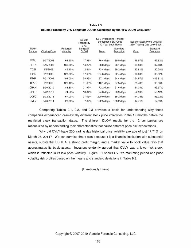
Copyright © 2007-2019 Vianello Forensic Consulting, LLC 168
Table 9.3
Double Probability VFC Longstaff DLOMs Calculated by the VFC DLOM Calculator
Ticker Symbol Closing Date
Reported Volatility
Double Probability
VFC Longstaff
DLOM
SEC Processing Time for the Issuer’s SIC Code (10 Year Look-Back)
Issuer’s Stock Price Volatility (250 Trading Day Look-Back)
Mean Standard Deviation Mean
Standard Deviation
WAL 6/27/2008 64.20% 17.98% 76.4 days 39.5 days 46.97% 42.82%
PRTK 8/15/2008 166.00% 14.22% 98.0 days 76.1 days 39.83% 97.48%
TCBI 9/8/2008 46.10% 12.41% 73.4 days 39.2 days 33.81% 30.38%
OPK 6/2/2009 128.30% 37.63% 104.6 days 92.4 days 92.63% 88.82%
FTGI 7/31/2009 493.00% 58.93% 87.1 days 64.4 days 254.97% 403.81%
TEAR 1/8/2010 126.10% 31.60% 110.1 days 57.5 days 75.43% 99.36%
CBAN 3/30/2010 88.80% 21.97% 72.2 days 51.6 days 61.24% 65.97%
BPFH 6/22/2010 74.50% 18.84% 74.6 days 68.9 days 52.59% 50.12%
UCFC 3/22/2013 67.00% 27.03% 200.0 days 65.2 days 44.38% 53.22%
CVLY 3/26/2014 26.00% 7.62% 122.5 days 138.2 days 17.71% 17.89%
Comparing Tables 9.1, 9.2, and 9.3 provides a basis for understanding why these
companies experienced dramatically different stock price volatilities in the 12 months before the
restricted stock transaction dates. The different DLOM results for the 12 companies are
rationalized by understanding their characteristics that cause different price risk expectations.
Why did CVLY have 250-trading day historical price volatility average of just 17.71% on
March 26, 2014? We can surmise that it was because it is a financial institution with substantial
assets, substantial EBITDA, a strong profit margin, and a market value to book value ratio that
approximates its book assets. Investors evidently agreed that CVLY was a lower-risk stock,
which is reflected in its low price volatility. Figure 9.1 shows CVLY’s marketing period and price
volatility risk profiles based on the means and standard deviations in Table 9.3.
[Intentionally Blank]

Copyright ©
Figure 9.2 shows CVLY’s double probability risk profile based on the combined risk
profiles of Figure 9.1. The peaked area represents the most likely combined occurrences
accounts for the lion’s share of CVLY’s 7.62% double probability VFC Longstaff DLOM shown in
Table 9.3.
Copyright © 2007-2019 Vianello Forensic Consulting, LLC 169
Figure 9.2 shows CVLY’s double probability risk profile based on the combined risk
9.1. The peaked area represents the most likely combined occurrences
accounts for the lion’s share of CVLY’s 7.62% double probability VFC Longstaff DLOM shown in
Figure 9.2 shows CVLY’s double probability risk profile based on the combined risk
9.1. The peaked area represents the most likely combined occurrences, and
accounts for the lion’s share of CVLY’s 7.62% double probability VFC Longstaff DLOM shown in

Copyright ©
Figure 9.3 is a two-dimensional display that shows in red the proportion
combined marketing period and price volatility probabilities that result in raw VFC Longstaff
DLOMs of 100%.
Figure 9.4 is a three dimensional display that shows in red the low probabilities
associated with CVLY’s combinations of marketing
result in VFC Longstaff DLOMs of 100%.
Copyright © 2007-2019 Vianello Forensic Consulting, LLC 170
dimensional display that shows in red the proportion
combined marketing period and price volatility probabilities that result in raw VFC Longstaff
Figure 9.4 is a three dimensional display that shows in red the low probabilities
associated with CVLY’s combinations of marketing period and price volatility probabilities that
result in VFC Longstaff DLOMs of 100%.
[Intentionally Blank]
dimensional display that shows in red the proportion of CVLY’s
combined marketing period and price volatility probabilities that result in raw VFC Longstaff
Figure 9.4 is a three dimensional display that shows in red the low probabilities
period and price volatility probabilities that

Copyright ©
Why did FTGI have historical price volatility of 254.97% on September 25, 2007? We
can surmise that it was because FTGI had negative preceding year EBITDA that was equal to its
preceding year revenues, 150% of its book equity, and over 40% of its assets.
evidently agreed that FTGI was a very risky stock. That risk was appropriately reflected in very
high stock price volatility. Figure 9.5 shows FTGI’s marketing period and price volatility risk
profiles based on the means and standard deviation
in the y axis of Figure scale and skewing of the probability lines compared to Figure 9.1
Figure 9.5 y axis scale is an order of magnitude greater than the Figure 9.1 scale
by FTGI’s much greater price volatility compared to CVLY’s.
scale of Figure 9.5 is half of the Figure 9.1 marketing period scale. These comparisons help
explain why the FTGI DLOM is 7.7 times the CVLY DLOM.
Copyright © 2007-2019 Vianello Forensic Consulting, LLC 171
Why did FTGI have historical price volatility of 254.97% on September 25, 2007? We
can surmise that it was because FTGI had negative preceding year EBITDA that was equal to its
preceding year revenues, 150% of its book equity, and over 40% of its assets.
evidently agreed that FTGI was a very risky stock. That risk was appropriately reflected in very
Figure 9.5 shows FTGI’s marketing period and price volatility risk
profiles based on the means and standard deviations in Table 9.3. Note the significant difference
in the y axis of Figure scale and skewing of the probability lines compared to Figure 9.1
Figure 9.5 y axis scale is an order of magnitude greater than the Figure 9.1 scale. This is caused
h greater price volatility compared to CVLY’s. But the marketing period x axis
scale of Figure 9.5 is half of the Figure 9.1 marketing period scale. These comparisons help
explain why the FTGI DLOM is 7.7 times the CVLY DLOM.
[Intentionally Blank]
Why did FTGI have historical price volatility of 254.97% on September 25, 2007? We
can surmise that it was because FTGI had negative preceding year EBITDA that was equal to its
preceding year revenues, 150% of its book equity, and over 40% of its assets. Investors
evidently agreed that FTGI was a very risky stock. That risk was appropriately reflected in very
Figure 9.5 shows FTGI’s marketing period and price volatility risk
s in Table 9.3. Note the significant difference
in the y axis of Figure scale and skewing of the probability lines compared to Figure 9.1—the
. This is caused
But the marketing period x axis
scale of Figure 9.5 is half of the Figure 9.1 marketing period scale. These comparisons help
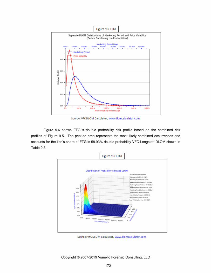
Copyright ©
Figure 9.6 shows FTGI’s double probability risk profile based on the combined risk
profiles of Figure 9.5. The peaked area represents the most likely combined occurrences and
accounts for the lion’s share of FTGI’s 58.93% double probability VFC Longsta
Table 9.3.
Copyright © 2007-2019 Vianello Forensic Consulting, LLC 172
Figure 9.6 shows FTGI’s double probability risk profile based on the combined risk
profiles of Figure 9.5. The peaked area represents the most likely combined occurrences and
accounts for the lion’s share of FTGI’s 58.93% double probability VFC Longstaff DLOM shown in
Figure 9.6 shows FTGI’s double probability risk profile based on the combined risk
profiles of Figure 9.5. The peaked area represents the most likely combined occurrences and
ff DLOM shown in

Copyright ©
Figure 9.7 is a two-dimensional display that shows in red the proportion of FTGI’s
combined marketing period and price volatility probabilities that result in raw VFC Longstaff
DLOMs of 100%. Note the significantly greater n
those for CVLY shown in Figure 9.3.
Figure 9.8 is a three dimensional display that shows in red the low probabilities
associated with FTGI’s combinations of marketing period and price volatility probabilities
result in VFC Longstaff DLOMs of 100%.
very low. The high-probability area
58.93% VFC Longstaff DLOM.
Copyright © 2007-2019 Vianello Forensic Consulting, LLC 173
dimensional display that shows in red the proportion of FTGI’s
combined marketing period and price volatility probabilities that result in raw VFC Longstaff
Note the significantly greater number of red combinations for FTGI compared
those for CVLY shown in Figure 9.3.
Figure 9.8 is a three dimensional display that shows in red the low probabilities
associated with FTGI’s combinations of marketing period and price volatility probabilities
result in VFC Longstaff DLOMs of 100%. Note that the probability of red combinations remains
probability area presented in green accounts for the lion’s share of FTGI’s
[Intentionally Blank]
dimensional display that shows in red the proportion of FTGI’s
combined marketing period and price volatility probabilities that result in raw VFC Longstaff
umber of red combinations for FTGI compared
Figure 9.8 is a three dimensional display that shows in red the low probabilities
associated with FTGI’s combinations of marketing period and price volatility probabilities that
Note that the probability of red combinations remains
for the lion’s share of FTGI’s

Copyright ©
Readers can consider whether
the relative price volatilities of the other stocks in the list.
VFC double probability DLOMs
square of correlation of the average price volatilities with the VFC Longstaff DLOMs is
With the understanding that DLOMs should represent the investment risk, it can be seen
that the VFC DLOM Calculator
volatility associated with the illiquid time periods required to sell investments
0%
10%
20%
30%
40%
50%
60%
70%
0% 50%
VF
C L
on
gsta
ff D
ou
ble
Pro
ba
bilit
y D
LO
M
Logarithmic Regression of Table
Copyright © 2007-2019 Vianello Forensic Consulting, LLC 174
Readers can consider whether the financial differences shown Tables 9.2 and 9.3
the relative price volatilities of the other stocks in the list. Figure 9.9 shows the correlation of the
VFC double probability DLOMs and underlying average price volatilities per Table
square of correlation of the average price volatilities with the VFC Longstaff DLOMs is
With the understanding that DLOMs should represent the investment risk, it can be seen
e VFC DLOM Calculator® yields DLOMs that are highly responsive to the risks of price
volatility associated with the illiquid time periods required to sell investments.
y = 0.2045ln(x) + 0.3681
R² = 0.9128
50% 100% 150% 200% 250% 300%
Price Volatility Mean
Figure 9.9
Logarithmic Regression of Table 9.3 VFC Mean Price Volatilities and DLOMs
shown Tables 9.2 and 9.3 explain
shows the correlation of the
per Table 9.3. The R-
square of correlation of the average price volatilities with the VFC Longstaff DLOMs is 91.28%.
With the understanding that DLOMs should represent the investment risk, it can be seen
the risks of price
300%
9.3 VFC Mean Price Volatilities and DLOMs

Copyright © 2007-2019 Vianello Forensic Consulting, LLC 175
Chapter 10
REVISITING “LITMAN AUDACITY”
Pluris®
president Espen Robak discussed the “wildly different discounts” presented to the
Federal Circuit court in a well-written analysis of the tax case Litman v. The United States.167
Litman in part dealt with the appropriate DLOM to apply to four tranches of Hotels.com restricted
stock issued to David Litman on February 24, 2000, coincident with the Hotels.com initial public
stock offering. Mr. Robak’s article includes a table that summarized the conflicting DLOM
opinions of the three valuation experts—one each for the IRS, Hotels.com, and Mr. Litman.
Table 10.1, which restates the information summarized in the Robak article, shows each expert’s
DLOM opinion for each tranche of stock, and the court’s corresponding conclusions:
Table 10.1
DLOM Estimates for HOTELS.COM Restricted Stock as of February 24, 2000
As Presented to and Decided by the Court
Tranche Restriction # of Shares Weight The IRS Hotels.com Litman The Court
One Year 1,959,960 20% 16.9% 20.0% 49.5% 22.0%
Two Years 489,990 5% 20.9% 20.0% 61.5% 36.0%
Three Years 489,990 5% 21.2% 20.0% 63.5% 38.0%
Four Years 7,059,960 70% 21.2% 20.0% 79.0% 50.0%
Total Shares 9,999,900
Weighted DLOM 100% 20.3% 20.0% 71.3% 43.0%
Litman provides an opportunity to demonstrate how DLOMs calculated using the VFC
DLOM Calculator® compare to those presented by the experts and decided by the Court. The
following parameters were selected for this demonstration:
• Valuation date: February 24, 2000.
• Guideline stock: The Priceline Group, Inc. (PCLN).
• PCLN price volatility look-back period = We attempted to obtain price data for the
250 trading days prior to the valuation date, but PCLN’s initial public offering
occurred just 36 trading days before the valuation date.
• PCLN price volatility: Average = 58.1%. Standard deviation = 44.5%.
• Source of marketing period data:168
VFC’s BIZCOMPS® database for SIC code
7389. Transactions that closed during the 10 years prior to the valuation date.
167
Litman v. The United States, Nos. 05-956T, 05-971T, 06-285T (August 22, 2007, modified March 20, 2008). 168
This demonstration assumes that registration of Mr. Litman’s shares was contractually prohibited, leaving only the possibility of a private sale. Therefore, the illiquidity time period is based on BIZCOMPS
® data instead of the processing time to obtain SEC registration.

Copyright © 2007-2019 Vianello Forensic Consulting, LLC 176
• Private sale marketing period probabilities: Average = 187.3 days. Standard
deviation = 140.2 days. Number of transactions = 76. Confidence interval =
155.8 days to 218.9 days.
• Application of SEC Rule 144 subsequent to the lock-up periods is ignored.
Lognormal distribution of the above price volatility was used in combination with the time
periods of the contractual restriction to calculate single probability DLOMs using the VFC
Longstaff and VFC Black-Scholes formulas of the VFC DLOM Calculator®. The assumption is
that each tranche would have been sold immediately at the end of its restriction period. Table
10.2 summarizes the calculated single-probability DLOMs.
Table 10.2
VFC DLOM Estimates for HOTELS.COM Restricted Stock as of February 24, 2000
Risk Free Rate = Zero; Dividend Rate = Zero
Single Probability 250-Day Pre-Closing Price Volatility Marketing Period = Tranche Restriction
Tranche Restriction VFC Longstaff VFC Black-Scholes The Court
One Year 50.7% 22.2% 22.0%
Two Years 65.4% 30.4% 36.0%
Three Years 73.6% 36.0% 38.0%
Four Years 79.0% 40.5% 50.0%
Weighted Average 72.3% 36.0% 43.0%
Table 10.2 shows that the single-probability VFC Black-Scholes DLOMs approximates
the Court’s tranche-based DLOM estimates, except that the Court’s DLOM estimate for the four-
year tranche is considerably higher than the single-probability VFC Black-Scholes estimate. The
weighted average of the Court’s DLOM estimates is 43% compared to the 36% weighted average
using the single-probability VFC Black-Scholes method. The single-probability VFC Black-
Scholes method appears to yield DLOM answers that the Court would have found to be
reasonable and acceptable.
Comparing Table 10.2 to Table 10.1 reveals that the single-probability VFC Longstaff
DLOMs very closely approximate the tranche-based opinions of Mr. Litman’s expert, who used a
CAPM method. The weighted average of Mr. Litman’s expert’s tranche-based DLOM estimates
is 71.3% (see Table 10.1) while the single-probability VFC Longstaff approach results in a
weighted average DLOM of 72.3% (see Table 10.2). Only the three-year tranche has
substantially different DLOM estimates. The single-probability VFC Longstaff method appears to
yield DLOM answers that Mr. Litman’s expert would have found to be reasonable and acceptable.

Copyright © 2007-2019 Vianello Forensic Consulting, LLC 177
The tranche conclusions of Mr. Litman’s expert correlate almost perfectly with the Court’s
tranche conclusions. The R-square of that correlation is 98%. The individual tranche DLOMs of
the single-probability VFC Longstaff formula also correlate highly with the court’s tranche
conclusions, with an R-square of 93%. Thus, the single-probability VFC Longstaff DLOMs are
corroborated by the opinions of Mr. Litman’s expert and the DLOM trends decided by the court.
Double-probability DLOMs are not tranche sensitive, because it is assumed that Mr.
Litman could have sold all 9,999,900 shares of Hotels.com stock that he owned in a private
transaction at any time. The period of time that it would take to find a private buyer and to
consummate the sale represents the alternative period of illiquidity associated with Mr. Litman’s
stock—that is, the probability of outcomes defined by private sales of SIC code 7389 businesses.
According to the VFC BIZCOMPS® database, this probability has a mean of about 194.6 days
and a standard deviation of about 152.2 days.
The double-probability DLOM calculated using the VFC Longstaff formula is 34.5%, while
the double-probability DLOM calculated using the VFC Black-Scholes formula is 15.1%. See
Table 10.3. With a value approximately midway between the IRS’s and Hotels.com’s weighted
average DLOMs on the one hand and the Court’s weighted average DLOM on the other hand, it
appears that the parties would have found the double probability VFC Longstaff DLOM result of
34.5% to be reasonable and acceptable.
Table 10.3
Double Probability 250-Day PCLN Price Volatility Marketing Period = BIZCOMPS
® SIC Code 7389
VFC Longstaff VFC Black-Scholes
34.5% 15.1%

Copyright © 2007-2019 Vianello Forensic Consulting, LLC 178
Chapter 11
CONCLUSIONS
Properly defined applications of the Longstaff, Black-Scholes, and Finnerty option
formulas can result in DLOMs that correlate highly with combinations of price volatility and
periods of illiquidity.169
Double probability VFC DLOMs representing the combined probabilities of
price and marketing period risks explained most of the variation the final set of analyzed restricted
stock discounts. Double probability DLOMs calculated using the Longstaff formula provided
values most consistent with the empirical evidence provided by the discounts of corresponding
restricted stock transactions. The calculated DLOMs should be considered systematic.
The currently available empirical information supports the conclusion that double
probability DLOMs calculated using the VFC Longstaff methodology results in reliable estimates
of systematic DLOM. The final analyzed set of transactions was necessarily limited by the
available data. The analyses presented in this research may be further refined if reliable price
data before 2007 becomes available and as more recent restricted stock transactions become
available to the author or other researchers.
Double probability DLOMs calculated using the VFC Black-Scholes formula tended to
understate the discounts of restricted stock transactions by about 50%. Double probability
DLOMs calculated using the VFC Finnerty formula tended to understate the discounts of
corresponding restricted stock transactions by about 85%. However, both correlated highly with
the reported discounts of the final set of analyzed transactions.
Important to valuation practitioners are the facts that (a) price data for currently listed
public companies is available daily, and (b) time data is available for a great many publicly traded
companies through the VFC public company filings database and for privately sold companies
through the BIZCOMPS® and DealStats
® databases. These factors allow practitioners to
calculate DLOMs using the option models that are highly specific to the valuation subject and the
valuation date. The research supports a conclusion that more objective, persuasive, and reliable
DLOMs can be developed using the VFC DLOM Calculator® methodology than by using
previously available methodologies.
Marc Vianello, CPA, ABV, CFF
July 1, 2019
169
Although not discussed in this research paper, the Finnerty formula was studied in the same manner as the Longstaff and Black-Scholes formulas. The Finnerty formula yielded comparable double probability regression results except for understating the reported restricted stock discounts of the final study set by a factor of about 7.

Copyright © 2007-2019 Vianello Forensic Consulting, LLC 179
Guide for Using the VFC DLOM Calculator®
Table of Contents
Page
Preface 180
Registration 182
My Account 183
My Projects 184
Creating a New Project 186
Updating Projects 189
Viewing Project Runs 190
Purchasing Credits 192
Using DLOM Calculators and Estimators 198
Types of Calculators and Estimators 198
Probability-Based Marketing Periods 201
Private Companies 202
Defining Private Company Marketing Periods 209
Defining Successful Public Offering Periods 210
Processing BIZCOMPS or Stout Transaction Selections 216
Using Specified Time Periods 219
Probability-Based Price Volatilities 219
DLOM Formula Selection 224
Understanding Calculator and Estimator Results 226
Limited Free Trial Mode 242

Copyright © 2007-2019 Vianello Forensic Consulting, LLC 180
Guide for Using the VFC DLOM Calculator® (July 2019)
Preface
The VFC DLOM Calculator® provides DLOM estimates using the Longstaff, Black-
Scholes, and Finnerty option formulas applied to weighted probabilities of price volatility and time
periods of illiquidity. The calculated DLOMs represent the full range of likely outcomes based on
the probability weightings.
Systematic price risk can be benchmarked on guideline company price data. Once a
user has selected one or more guideline companies and specified a price reference time period,
the VFC DLOM Calculator® calculates price risk probabilities using daily price data obtained from
NASDAQ and AlphaVantage. Alternatively, price volatility assumptions consisting of an average
and a standard deviation of price volatility can be provided by the user.
For most businesses and securities that are not publicly traded, the time required to
market the investment represents the period of illiquidity. Marketing period probabilities for
privately held businesses can be observed in the transactions reported in the BIZCOMPS® and
Pratt’s Stats® databases and in the approval times required to process public offerings through
the SEC. The VFC DLOM Calculator® maintains a database of BIZCOMPS
® transactions that
users can access for private company marketing period estimation. The VFC DLOM Calculator®
also maintains a proprietary database of SEC Form S-1 filings from which SEC processing times
are calculated. Users can access this database for public offering processing time estimation.
Alternatively, users can develop their own time period probability assumptions using their
BIZCOMPS® or Pratt’s Stats
® subscriptions or from other sources. Such user-provided
probability assumptions consist of an average and a standard deviation of time periods.
To calculate probability-based DLOM, the price volatility and time period data are divided
into segments based on the standard log-normal distribution that results from the assumptions of
average and standard deviation developed from the specified guideline companies and private
sale transactions. A combined probability distribution is then developed that represents the range
of probability combinations of price and time occurrences. The VFC DLOM Calculator® then
calculates a DLOM for each combination of price volatility and time using the option formula
chosen by the user. The currently available option formulas are Longstaff, Black-Scholes, and
Finnerty. The DLOMs are next multiplied by the probability associated with each combination of
marketing period and price volatility to produce a probability weighted DLOM. These probabilities
are re-weighted so that the total probability is 100%. The probability weighted DLOMs for all the
marketing period and price volatility combinations are summed to produce a double probability
weighted DLOM for the asset.

Copyright © 2007-2019 Vianello Forensic Consulting, LLC 181
Single probability DLOMs will be calculated if the user chooses to use probability for only
one of marketing period or price volatility. A single probability DLOM would be appropriate in
circumstances in which a fixed time period of liquidity is known or determinable but the asset
price remains volatile, or if an asset price is constant over a marketing time period that is variable.
For example, a security may have a restriction on sale that, upon expiration, allows the immediate
sale to a buyer at the then market price. Or the price of an asset may be fixed contractually while
being offered for sale but still requires an unknown amount of time to consummate a sale. In
such circumstances, the DLOM will be calculated and probability weighted for whichever variable
is using the probability distribution. The other variable will remain will be fixed at the user-entered
value for the DLOM calculation for each segment. The results are summed up to get the single
probability weighted DLOM for the asset.

Copyright ©
Registration
Enter your email address, password, complete the captcha and click “Register
Registration is free.
Copyright © 2007-2019 Vianello Forensic Consulting, LLC 182
Enter your email address, password, complete the captcha and click “RegisterEnter your email address, password, complete the captcha and click “Register.”

Copyright ©
My Account
On this page you can manage your account or log out. The following navigation
options are available:
• Dashboard
o The current page
• My Projects
o You can manage your Projects
o You may also access this page by hovering your mouse over the “My
Account” panel in the navigation bar.
• My Orders
o You can view your order history and receipts
• Edit Account
o You can change your first name, last name, display name, email address,
and password
• Edit Billing Address
o You can modify your billing address
Copyright © 2007-2019 Vianello Forensic Consulting, LLC 183
On this page you can manage your account or log out. The following navigation
current page.
manage your Projects from this page.
You may also access this page by hovering your mouse over the “My
panel in the navigation bar.
u can view your order history and receipts at this page.
ou can change your first name, last name, display name, email address,
and password at this page.
ou can modify your billing address at this page.
On this page you can manage your account or log out. The following navigation
You may also access this page by hovering your mouse over the “My
ou can change your first name, last name, display name, email address,

Copyright ©
My Projects
To use the complete version of any of the
have both a Project and specific credits for the calculations you want to conduct. From
this page you can navigate to any of the
trials. Use the links labeled “Buy More
your cart.
You can view and edit any of your Projects by selecting them from the dropdown
located in the “My Existing Project
Copyright © 2007-2019 Vianello Forensic Consulting, LLC 184
To use the complete version of any of the Calculators and Estimators
have both a Project and specific credits for the calculations you want to conduct. From
this page you can navigate to any of the Calculators, Estimators and their respective free
trials. Use the links labeled “Buy More” to navigate to the Shop page to add credits to
You can view and edit any of your Projects by selecting them from the dropdown
located in the “My Existing Projects” box. You can then edit Project information by
Estimators you must
have both a Project and specific credits for the calculations you want to conduct. From
and their respective free
age to add credits to
You can view and edit any of your Projects by selecting them from the dropdown
box. You can then edit Project information by

Copyright © 2007-2019 Vianello Forensic Consulting, LLC 185
clicking the corresponding “Edit Project Profile” button. To view all of the prior
calculations performed and saved for a Project, click “View Run History.”

Copyright ©
Creating a New Project
On the My Projects page, you may click “Create New Projec
page where you can fill in a form describing
The “Subject Profile”
asset being evaluated. The “Appraiser Profil
the evaluation. The “Valuation Subject“ and “Valua
only be set once, they cannot be changed after a Project is created
may be edited. This profile information will be displayed along with your calculation
results, and in any report that you print.
The “Valuation Date“is particularly important for the Price Volatility tool. If you
want to use a custom price volatility period, you will be limited to 180 days before and
after the valuation date, as shown below:
Copyright © 2007-2019 Vianello Forensic Consulting, LLC 186
Creating a New Project
On the My Projects page, you may click “Create New Project” to navigate to a
page where you can fill in a form describing your subject and appraiser Profiles.
corresponds to the information of a company or other
asset being evaluated. The “Appraiser Profile” corresponds to the appraiser conducting
the evaluation. The “Valuation Subject“ and “Valuation Date“ are required and can
they cannot be changed after a Project is created. All other details
may be edited. This profile information will be displayed along with your calculation
results, and in any report that you print.
The “Valuation Date“is particularly important for the Price Volatility tool. If you
want to use a custom price volatility period, you will be limited to 180 days before and
after the valuation date, as shown below:
to navigate to a
your subject and appraiser Profiles.
corresponds to the information of a company or other
corresponds to the appraiser conducting
tion Date“ are required and can
. All other details
may be edited. This profile information will be displayed along with your calculation
The “Valuation Date“is particularly important for the Price Volatility tool. If you
want to use a custom price volatility period, you will be limited to 180 days before and

Copyright ©
Here is an example of a completed N
The screenshot below corresponds to the aspects of your Project to be displayed
when your results are calculated.
Copyright © 2007-2019 Vianello Forensic Consulting, LLC 187
Here is an example of a completed New Project page:
The screenshot below corresponds to the aspects of your Project to be displayed
when your results are calculated.
The screenshot below corresponds to the aspects of your Project to be displayed

Copyright ©
The next screenshot demonstrates the aspects of your Project to be displayed on
the first page of every report that y
Copyright © 2007-2019 Vianello Forensic Consulting, LLC 188
screenshot demonstrates the aspects of your Project to be displayed on
the first page of every report that you print.
screenshot demonstrates the aspects of your Project to be displayed on

Copyright ©
Updating Projects
You can change any aspect of the Profiles, except for the “Valuation Subject” and
“Valuation Date” by selecting a Project from the dropdown on the “My Projects” page,
and clicking “edit Project Profile.” After you have m
Project.” If for any reason you wish to delete your Project you may click “Delete Project”
and confirm the prompt. Be aware that if you delete a Project, all Runs and associated
data will be lost and unrecoverable.
Copyright © 2007-2019 Vianello Forensic Consulting, LLC 189
You can change any aspect of the Profiles, except for the “Valuation Subject” and
“Valuation Date” by selecting a Project from the dropdown on the “My Projects” page,
and clicking “edit Project Profile.” After you have made your changes, click “Update
Project.” If for any reason you wish to delete your Project you may click “Delete Project”
and confirm the prompt. Be aware that if you delete a Project, all Runs and associated
data will be lost and unrecoverable.
You can change any aspect of the Profiles, except for the “Valuation Subject” and
“Valuation Date” by selecting a Project from the dropdown on the “My Projects” page,
ade your changes, click “Update
Project.” If for any reason you wish to delete your Project you may click “Delete Project”
and confirm the prompt. Be aware that if you delete a Project, all Runs and associated

Copyright ©
Viewing Project Runs
Anytime you initiate a calculation on a Calculator or Estimator, you are executing
a “Run.” The information generated from the Run is automatically stored for later
viewing. On the “My Projects” page, after selecting a Project from the dr
“View Run History” view all Runs associated with the Project.
The Runs table displays all of the archived Runs for a Project. If you want to view
the full results of a specific Run, click the blue “View” button that appears on the right
side of each row. If you click the green “+” button to the right of the “View”
will be given more options. Mobile users may tap the row itself to view these options.
Clicking the “View Run” button
The “Print Report” button will show the PDF report results associated with any
particular Run.
Copyright © 2007-2019 Vianello Forensic Consulting, LLC 190
ng Project Runs
Anytime you initiate a calculation on a Calculator or Estimator, you are executing
The information generated from the Run is automatically stored for later
viewing. On the “My Projects” page, after selecting a Project from the dropdown, click
“View Run History” view all Runs associated with the Project.
The Runs table displays all of the archived Runs for a Project. If you want to view
the full results of a specific Run, click the blue “View” button that appears on the right
side of each row. If you click the green “+” button to the right of the “View”
will be given more options. Mobile users may tap the row itself to view these options.
button also allows you to view the full results.
The “Print Report” button will show the PDF report results associated with any
Anytime you initiate a calculation on a Calculator or Estimator, you are executing
The information generated from the Run is automatically stored for later
opdown, click
The Runs table displays all of the archived Runs for a Project. If you want to view
the full results of a specific Run, click the blue “View” button that appears on the right
side of each row. If you click the green “+” button to the right of the “View” button, you
will be given more options. Mobile users may tap the row itself to view these options.
The “Print Report” button will show the PDF report results associated with any

Copyright © 2007-2019 Vianello Forensic Consulting, LLC 191
The “Delete Run” button will allow you to delete the Run from the archive. After
a Run is deleted, it cannot be recovered. If you want to hide these options, you may
click the same green “+” button to do so.
All Runs can be “Saved” on their full results page. Run views can be limited to
only the “Saved” Runs by typing “Saved” into the search box in the top right corner. The
search box can also be used with other text queries to view only Runs that satisfy the
query.

Copyright ©
Purchasing Credits
Navigate to the Shop page by clicking the “Shop” panel in the horizontal
navigation bar.
Copyright © 2007-2019 Vianello Forensic Consulting, LLC 192
Navigate to the Shop page by clicking the “Shop” panel in the horizontal Navigate to the Shop page by clicking the “Shop” panel in the horizontal

Copyright © 2007-2019 Vianello Forensic Consulting, LLC 193
In the shop you can buy Run credits for the Calculators and Estimators, buy Look-
Up credits for Price Volatility Research, and buy Valuation Project Packs. A Valuation
Project Pack is a complete use package that contains multiple Run credits, multiple
Look-Up credits and a Project credit. Credits are global, meaning that any Run credits or
Look-Up credit can be applied to any Project that you have created.
One Project Package includes:
• 1 Project Credit
• 10 Double Probability DLOM Run Credits
• 10 Single Probability DLOM Run Credits
• 10 Marketing Period Estimator Run Credits
• 10 Price Volatility Estimator Run Credits
• 30 Price Volatility Research Look-Up Credits
Successful Price Volatility Look-Ups are cached and available for unlimited usage for 336
hours.
Click a product image on the Shop page to get more information about the
particular product. Click the “Add to cart” button to add products your shopping cart.

Copyright ©
To view your shopping cart, click the “Cart” panel in the horizontal navigation
bar. On this page you can remove items from your Cart, apply coupon codes, and to set
the quantity of items you wish to purchase. Once you are ready to purchase click the
“Proceed to checkout” button.
Copyright © 2007-2019 Vianello Forensic Consulting, LLC 194
To view your shopping cart, click the “Cart” panel in the horizontal navigation
bar. On this page you can remove items from your Cart, apply coupon codes, and to set
the quantity of items you wish to purchase. Once you are ready to purchase click the
heckout” button.
To view your shopping cart, click the “Cart” panel in the horizontal navigation
bar. On this page you can remove items from your Cart, apply coupon codes, and to set
the quantity of items you wish to purchase. Once you are ready to purchase click the

Copyright ©
On the checkout page you need to fill in your billing information and check the
box signifying that you have
PayPal” button when you are ready to pay
information and click the “Pay Now“ button,
use on any of your Projects, assuming no transaction failures. You can check your “My
Projects” page to confirm that
account. You can also access your receipts by navigating to the “My Accoun
clicking “My Orders.”
Copyright © 2007-2019 Vianello Forensic Consulting, LLC 195
On the checkout page you need to fill in your billing information and check the
read the Terms and Conditions. Click the “Proceed to
when you are ready to pay. Once you have completed entering your
information and click the “Pay Now“ button, credits will be immediately available for
, assuming no transaction failures. You can check your “My
that your purchased credits were properly added to your
access your receipts by navigating to the “My Accoun
On the checkout page you need to fill in your billing information and check the
lick the “Proceed to
leted entering your
be immediately available for
, assuming no transaction failures. You can check your “My
were properly added to your
access your receipts by navigating to the “My Account” page and

Copyright ©
Copyright © 2007-2019 Vianello Forensic Consulting, LLC 196

Copyright ©
Copyright © 2007-2019 Vianello Forensic Consulting, LLC 197

Copyright © 2007-2019 Vianello Forensic Consulting, LLC 198
Using DLOM Calculators and Estimators
Types of Calculators and Estimators
There are two Calculators and two Estimators available to users. Each Calculator
and Estimator requires a payment using a Run credit. Each DLOM Calculator and
Estimator serves a unique purpose while utilizing a common set of tools. A variable
marketing period requires a mean and standard deviation, while a static marketing
period requires just a mean. Variable price volatility requires a mean and standard
deviation, while static price volatility requires just a mean. VFC DLOM Calculator
provides specialized tools to generate marketing period and price volatility means and
standard deviations for calculating DLOMs and estimating parameters. This guide will
first explain the common set of tools used by the Calculators and Estimators, and how to
use them. Afterwards, this guide will explain what tool each Calculator and Estimator
uses, and what results will be provided from a single Run.
Calculators
• Double Probability DLOM Calculator
o This Calculator utilizes both the Marketing Period Input and Price
Volatility tools to get two sets of mean and standard deviations to
calculate a double probability DLOM.
• Single Probability DLOM Calculator
o This Calculator has two modes both of which are accessible on the same
Calculator page.
� Static Marketing Period with a Price Volatility mean and standard
deviation to calculate a single probability DLOM
� Static Price Volatility with a Marketing Period mean and standard
deviation to calculate a single probability DLOM
Estimators
• Marketing Period Estimator
o Uses only the Marketing Period Tools

Copyright ©
• Price Volatility Estimator
o Uses only the Price Volatility Tools
Single Probability DLOM Calculator Static Tools
This Calculator has two modes both
page. You can select the “Metho
The “Use Variable Marketing Period with Fixed Price Volatility“ option allows
users to (a) use the Marketing Period Input tool to generate marketing period values
and (b) input a number that represents the average Price Volatility.
Copyright © 2007-2019 Vianello Forensic Consulting, LLC 199
Volatility Estimator
Uses only the Price Volatility Tools
Single Probability DLOM Calculator Static Tools
has two modes both, which are accessible on the same
page. You can select the “Method” to set the mode of the Calculator.
The “Use Variable Marketing Period with Fixed Price Volatility“ option allows
use the Marketing Period Input tool to generate marketing period values
input a number that represents the average Price Volatility.
hich are accessible on the same Calculator
The “Use Variable Marketing Period with Fixed Price Volatility“ option allows
use the Marketing Period Input tool to generate marketing period values,

Copyright ©
The “Use Variable Price Volatility with Fixed Marketing Period“ option allows
users to (a) use the Price Volatility tool to generate price volatility values
number that represents the number of marketing days.
Copyright © 2007-2019 Vianello Forensic Consulting, LLC 200
The “Use Variable Price Volatility with Fixed Marketing Period“ option allows
use the Price Volatility tool to generate price volatility values, and
number that represents the number of marketing days.
The “Use Variable Price Volatility with Fixed Marketing Period“ option allows
and (b) input a

Copyright ©
Probability-Based Marketing Periods
This tool allows users to generate a marketing period mean and standard
deviation. Credits are not required
• Private Companies
o This choice bases marketing period estimates on BIZCOMPS® transactions
comprising the VFC
are over 16,000 transactions in our database.
• Successful Public Offerings
o This choice bases marketing period estimates on benchmarks selected
from the SEC filings comprising the VFC DLOM Calculator® success
Copyright © 2007-2019 Vianello Forensic Consulting, LLC 201
ing Periods
This tool allows users to generate a marketing period mean and standard
are not required to use this tool.
This choice bases marketing period estimates on BIZCOMPS® transactions
comprising the VFC DLOM Calculator® private company database.
000 transactions in our database.
Successful Public Offerings
This choice bases marketing period estimates on benchmarks selected
from the SEC filings comprising the VFC DLOM Calculator® success
This tool allows users to generate a marketing period mean and standard
This choice bases marketing period estimates on BIZCOMPS® transactions
DLOM Calculator® private company database. There
This choice bases marketing period estimates on benchmarks selected
from the SEC filings comprising the VFC DLOM Calculator® successful

Copyright © 2007-2019 Vianello Forensic Consulting, LLC 202
public offering database. There are over 10,000 SEC filings in our
database.
• Process BIZCOMPS® or Stout (formerly Pratt’s Stats®) Selection
o This choice bases marketing period estimates on specific transactions
that you select using your BIZCOMPS® or Stout subscription, and upload
to the VFC DLOM Calculator®.
• Provide Your Own Time Factors
o This choice bases marketing period estimates on a marketing period
mean and standard distribution that you have developed from other
sources.
Private Companies
This choice bases marketing period estimates on the averages of all or subsets of
the BIZCOMPS® transactions comprising the VFC DLOM Calculator® private company
database. To view the mean and standard deviation your selection generates, click the
“Display Marketing Period” button.
Use Entire Database
This choice utilizes the entire set of BIZCOMPS® transactions in our database, as
shown in the screenshot below.
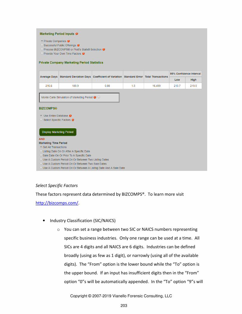
Copyright ©
Select Specific Factors
These factors represent data determined by
http://bizcomps.com/.
• Industry Classification
o You can set a range between two SIC or NAICS numbers representing
specific business
SICs are 4 digits and all NAICS are 6 digits.
broadly (using as few as 1 digit), or narrowly (using all of the available
digits). The “Fro
the upper bound. If an input has insufficient digits then in the “Fro
option “0”s will be automatically appended
Copyright © 2007-2019 Vianello Forensic Consulting, LLC 203
data determined by BIZCOMPS®. To learn more visit
Classification (SIC/NAICS)
set a range between two SIC or NAICS numbers representing
specific business industries. Only one range can be used at a time. All
SICs are 4 digits and all NAICS are 6 digits. Industries can be defined
broadly (using as few as 1 digit), or narrowly (using all of the available
The “From” option is the lower bound while the “To”
the upper bound. If an input has insufficient digits then in the “Fro
option “0”s will be automatically appended. In the “To” option “9”s will
visit
set a range between two SIC or NAICS numbers representing
. Only one range can be used at a time. All
Industries can be defined
broadly (using as few as 1 digit), or narrowly (using all of the available
o” option is
the upper bound. If an input has insufficient digits then in the “From”
option “9”s will

Copyright © 2007-2019 Vianello Forensic Consulting, LLC 204
be automatically appended if fewer than all digits are used in the industry
range definition.
• State/Region
o This factor allows you to set one or multiple geographic locations as a
parameter. The locations are as reported by BIZCOMPS®.
• Slider Factors. These factors utilize a slider bar representing a range of values
allowed for the factor. The slider does not appear unless the factor is checked; if
unchecked the slider will disappear.
o Asking Price. This factor corresponds to the “ASK PRICE” field in
BIZCOMPS®.
o Annual Gross. This factor corresponds to the “ANN GROSS” field in
BIZCOMPS®.
o Number of Employees. This factor corresponds to the “# of EMPL” field
in BIZCOMPS®. BIZCOMPS® reports the number of both full time and part
time employees is given, for simplicity these numbers are summed for a
total number of employees. We are not able to convert the BIZCOMPS®
information to full-time equivalent employee counts.

Copyright ©
Statistics Table
There are statistics associated with the marketin
The marketing period statistics are: average number of days on the market; t
standard deviation of the number of days on the market; the coefficient of variation of
the number of days on the market; the standard error of the defined population; the
transaction count of the defined population; and the 95% confidence interval for
defined population.
Using Multiple Factors
Copyright © 2007-2019 Vianello Forensic Consulting, LLC 205
There are statistics associated with the marketing period factors that you select.
The marketing period statistics are: average number of days on the market; t
standard deviation of the number of days on the market; the coefficient of variation of
the number of days on the market; the standard error of the defined population; the
transaction count of the defined population; and the 95% confidence interval for
period factors that you select.
The marketing period statistics are: average number of days on the market; the
standard deviation of the number of days on the market; the coefficient of variation of
the number of days on the market; the standard error of the defined population; the
transaction count of the defined population; and the 95% confidence interval for the

Copyright © 2007-2019 Vianello Forensic Consulting, LLC 206
If you use only a single factor, then you will be given only one standard deviation
and average. However, if you use multiple factors you will be given the opportunity to
use different methods to generate an ultimate standard deviation and average.
• Weighted Average of Factors.
o This option is selected by default.
o This choice bases your marketing period conclusion on the weighted
average mean and standard deviation of marketing period days for the
defined populations of private sale transactions. Each transaction
possesses at least one of the characteristics that you selected.
Transactions possessing more than one characteristic are counted in each
defined sub-population. This choice results in the broadest measure
mean and standard deviation.
• Average of Unique Transactions
o This choice bases your marketing period conclusion on the simple
average mean and standard deviation of marketing period days for the
unique private sale transactions. Each transaction possesses at least one
of the characteristics that you selected, but each transaction is
considered only once. This choice results in a more restrictive measure
of mean and standard deviation than the weighted average choice.
• Transactions With All Factors
o This choice bases your marketing period conclusion on the simple
average mean and standard deviation of marketing period days for the
private sale transactions with all the characteristics that you selected.
This choice results in the most restrictive measure of mean and standard
deviation.
Results Graphs
You can view graphs that display information about your one or more factors to
allow visual comparison of the differences between them.

Copyright © 2007-2019 Vianello Forensic Consulting, LLC 207
• Relative Precision
• Mean
• Standard Deviation
• Datapoint Count
• Standard Error

Copyright ©
Copyright © 2007-2019 Vianello Forensic Consulting, LLC 208

Copyright ©
Defining Private Company Marketing Period
Defining a time period allows you to further refine the
transactions for calculating time period means and standard deviations. This can be
done using either Sale Dates or Listing Dates.
transaction data, but does not provide a Listing Date. Nevertheless, the VFC DLOM
Calculator® generates Listing Dates by
provided in BIZCOMPS® spreadsheets from the Sale Date.
database is 1/31/1986, and the
8/4 /1985 and the latest is currently
added to our database, the latest Listing and Sale Dates will advance.
• Get All Transactions.
o This selection uses all available transactions with the selection factors
that you defined.
• Listing Date On or After
o This selection uses all available transactions with the selection factors
that you defined that were listed
• Sale Date On or Prior
o This selection uses all available transactions with the selection factors
that you defined that sold
• Use a Custom Period On or Between Two Listing
Copyright © 2007-2019 Vianello Forensic Consulting, LLC 209
Marketing Periods
ime period allows you to further refine the selection of BIZCOMPS®
transactions for calculating time period means and standard deviations. This can be
done using either Sale Dates or Listing Dates. BIZCOMPS® provides a Sale Date with its
transaction data, but does not provide a Listing Date. Nevertheless, the VFC DLOM
Calculator® generates Listing Dates by subtracting the number of “DAYS ON MK
provided in BIZCOMPS® spreadsheets from the Sale Date. The oldest Sale Dat
and the latest is currently 7/13/2015. The oldest Listing Dat
currently 6/13/2015. As more BIZCOMPS® transactions are
added to our database, the latest Listing and Sale Dates will advance.
selection uses all available transactions with the selection factors
that you defined.
r After a Specific Date.
This selection uses all available transactions with the selection factors
that you defined that were listed on or after the Listing Date you
Prior to a Specific Date.
This selection uses all available transactions with the selection factors
that you defined that sold on or before the Sale Date you specif
Use a Custom Period On or Between Two Listing Dates.
BIZCOMPS®
transactions for calculating time period means and standard deviations. This can be
provides a Sale Date with its
transaction data, but does not provide a Listing Date. Nevertheless, the VFC DLOM
subtracting the number of “DAYS ON MKT”
Sale Date in our
7/13/2015. The oldest Listing Date is
As more BIZCOMPS® transactions are
selection uses all available transactions with the selection factors
This selection uses all available transactions with the selection factors
sting Date you specify.
This selection uses all available transactions with the selection factors
specify.

Copyright © 2007-2019 Vianello Forensic Consulting, LLC 210
o This selection uses all available transactions with the selection factors
that you defined that were listed on or between the Listing Dates you
specify.
• Use a Custom Period On or Between Two Sale Dates.
o This selection uses all available transactions with the selection factors
that you defined that were sold on or between the Sale Dates you
specify.
• Use a Custom Period On or Between a Listing Date and a Sale Date.
o This selection uses all available transactions with the selection factors
that you defined that were listed on or after the Listing Date that you
specify and were sold on or before the Sale Date that you specify.
Defining Successful Public Offering Periods
This option provides you a selection from three different transaction types for
estimating marketing periods for larger businesses—those suitable for a public equity
offerings–and other types of publicly registered securities. The types of transactions
are:
• Equity
• Notes
• Mixed Securities
Once a transaction type has been selected you may further refine you analysis by
specifying a specific SIC Code or a range of codes. SIC Code and transaction dates, or
ranges thereof, are the only transaction parameters available for estimating Public
Offering time periods.
If no SIC Code or range is specified, the VFC DLOM Calculator® will use all of the
transactions in the database that satisfy your specified date parameters to calculate the
Marketing Period mean and standard deviation. Similarly, f no date or date range is
specified, the VFC DLOM Calculator® will use all of the transactions in the database that

Copyright ©
satisfy your specified SIC Code parameters to calculate the Marketing Period mean and
standard deviation.
Click the “Display Marketing Per
screenshot below demonstrates the presentation.
Copyright © 2007-2019 Vianello Forensic Consulting, LLC 211
satisfy your specified SIC Code parameters to calculate the Marketing Period mean and
lick the “Display Marketing Period” button to view the calculation results. The
screenshot below demonstrates the presentation.
satisfy your specified SIC Code parameters to calculate the Marketing Period mean and
calculation results. The

Copyright ©
As previously explained,
into the “From” and “To” fields
has less than 4 digits it will automatically, append “0”s for “Fro
order to complete the range.
Copyright © 2007-2019 Vianello Forensic Consulting, LLC 212
As previously explained, you can select industry factors by entering SIC codes
fields shown in the screen shot below. Note that if a SIC
has less than 4 digits it will automatically, append “0”s for “From” and “9”s for “To”
.
factors by entering SIC codes
if a SIC Code
and “9”s for “To” in

Copyright ©
Successful Public Offerings Marketing Time Period
A marketing time period allows you to further refine the time frame f
S-1 filings should be counted.
Copyright © 2007-2019 Vianello Forensic Consulting, LLC 213
Successful Public Offerings Marketing Time Period
A marketing time period allows you to further refine the time frame f
1 filings should be counted.
A marketing time period allows you to further refine the time frame for when SIC

Copyright © 2007-2019 Vianello Forensic Consulting, LLC 214
A “Filing Date” falls on the date in which a Form S-1 was filed to the SEC. A “SEC
Approval Date” falls on the date on which a 424B1 or 424B4 was filed representing SEC
approval. The Marketing Days then is represented in the number of days falling on and
between the two filing dates. A mean and standard deviation is calculated based on the
transactions that satisfy all selected requirements. The first Form S-1 filing found is
dated 1994-01-07, and the currently latest filing is dated 2015-10-19. The first SEC
approval is dated 1994-04-07 and the currently latest SEC approval is dated 2015-10-19.
The VFC DLOM Calculator® is updated periodically to capture new Form A-1 filings and
SEC approvals. All time periods are inclusive, meaning that they include the days on the
“Filing Date” and “SEC Approval Date.”
• Get All Transactions.
o This selection uses all available transactions with the selection factors
that you defined.
• Filing Date After a Specific Date.
o This selection uses all available transactions with the selection factors
that you defined for which a Form S-1 was filed on or after the Filing Date
you specify.
• SEC Approval Date On or Prior to a Specific Date.
o This selection uses all available transactions with the selection factors
that you defined for which a Form 424B1 or 424B4 was approved on or
before the SEC Approval Date you specify.
• Use A Custom Period On or Between Two Filing Dates.
o This selection uses all available transactions with the selection factors
that you defined for which a Form S-1 was filed on or between the Filing
Dates you specify.
• Use A Custom Period On or Between Two SEC Approval Dates.
o This selection uses all available transactions with the selection factors
that you defined for which a 424B2 or 424B4 were filed on or between

Copyright ©
the SEC Approval Dates you
• Use A Custom Period On or Between a Filing Date and a
o This selection uses all available
that you defined for which a Form S
that you specify and for which a Form 424B2 or 424B4 was filed on
before the SEC Ap
Copyright © 2007-2019 Vianello Forensic Consulting, LLC 215
SEC Approval Dates you specify.
Use A Custom Period On or Between a Filing Date and a SEC Approval Date
This selection uses all available transactions with the selection factors
that you defined for which a Form S-1 was filed on or after the Filing Date
that you specify and for which a Form 424B2 or 424B4 was filed on
before the SEC Approval Date that you specify.
SEC Approval Date.
with the selection factors
1 was filed on or after the Filing Date
that you specify and for which a Form 424B2 or 424B4 was filed on or

Copyright ©
Monte Carlo Simulation of Marketing Period
Monte Carlo simulation
Company transactions and Successful Public Offerings. It allows you to override the
“Average Days” of the analytical population using
confidence interval. Standard deviations remain the same.
is run, a fourth column titled “User
results to show the effects of
Processing BIZCOMPS® or Stout Transaction
This option allows you to
calculating a marketing mean and standard deviation.
Stout subscription to use this function.
the blue button shown in the screenshot
Processed transactions are not retained by VFC DLOM Calculator. Be sure to
save your file. Only XLSX, XLS, and CSV Files are valid.
(approximately 1000 rows).
this may result in processing errors.
CSV Files
CSV files must have values delimite
encapsulated with quotes (“ ”
Copyright © 2007-2019 Vianello Forensic Consulting, LLC 216
Monte Carlo Simulation of Marketing Period
Monte Carlo simulation is available for the Marketing Periods of both Private
and Successful Public Offerings. It allows you to override the
of the analytical population using any number within the 95%
Standard deviations remain the same. After a Monte Carlo analysis
d “User Adjusted Average” will be displayed in the Run
the effects of the changed average.
Stout Transaction Selections
This option allows you to select a BIZCOMPS® or Stout spreadsheet file for use in
calculating a marketing mean and standard deviation. You must have a BIZCOMPS®
Stout subscription to use this function. If you do not have a BIZCOMPS®, please click
shown in the screenshot below to navigate to the BIXCOMPS® web
Processed transactions are not retained by VFC DLOM Calculator. Be sure to
your file. Only XLSX, XLS, and CSV Files are valid. The maximum file size is 2MB
(approximately 1000 rows). Please do not put line breaks (new lines) in your cells, as
this may result in processing errors.
CSV files must have values delimited by a comma (,) and text values should be
“ ”).
both Private
and Successful Public Offerings. It allows you to override the
any number within the 95%
a Monte Carlo analysis
in the Run
spreadsheet file for use in
You must have a BIZCOMPS® or
a BIZCOMPS®, please click
BIXCOMPS® website.
Processed transactions are not retained by VFC DLOM Calculator. Be sure to
maximum file size is 2MB
breaks (new lines) in your cells, as
d by a comma (,) and text values should be

Copyright © 2007-2019 Vianello Forensic Consulting, LLC 217
Header Row
The header row should be included for BIZCOMPS® or Pratt's Stats® selections.
For BIZCOMPS® the first row must have a cell with the contents “days on market.” For
Pratt's Stats® the first row must have two cells with one containing “Sale Initiation” and
another containing “Sale Date.” Once located, the entire column will be used for
Marketing Period calculations.
The header cells are not case sensitive, “days on market” and “DAYS ON
MARKET” are both valid.
Warnings
After the necessary columns are found, each row is processed individually. This
processing checks for valid syntax. "Days on market” values must be a number, while
"Sale Initiation” and "Sale Date” values must be dates in mm/dd/yyyy format.
If a "Sale Initiation” date occurs after a "Sale Date“ it is considered invalid,
otherwise the marketing period calculated for that row is the difference in days
between "Sale Date” and "Sale Initiation.”

Copyright ©
Using Specified Time Factors
Copyright © 2007-2019 Vianello Forensic Consulting, LLC 218
Time Factors

Copyright ©
This option allows you to enter your own Marketing Period mean and standard
deviation.
Probability-Based Price Volatili
This tool is provided to
• Use Publicly Traded Stocks or Indexes to Determine Price Volatility
o This choice bases price volatility estimates on user
indexes. The VFC DLOM Calculator® automatically calculates the price
volatility characteristics of the specified stocks and i
• Provide Your Own Price Volatility Factors
o This choice bases price volatility estimates on a distribution (mean and
standard deviation) that you developed from other sources.
Copyright © 2007-2019 Vianello Forensic Consulting, LLC 219
This option allows you to enter your own Marketing Period mean and standard
Based Price Volatilities
is provided to generate a price volatility mean and standard deviation.
Traded Stocks or Indexes to Determine Price Volatility
This choice bases price volatility estimates on user-specified stocks and
indexes. The VFC DLOM Calculator® automatically calculates the price
volatility characteristics of the specified stocks and indexes.
Provide Your Own Price Volatility Factors
This choice bases price volatility estimates on a distribution (mean and
standard deviation) that you developed from other sources.
This option allows you to enter your own Marketing Period mean and standard
generate a price volatility mean and standard deviation.
specified stocks and
indexes. The VFC DLOM Calculator® automatically calculates the price
This choice bases price volatility estimates on a distribution (mean and

Copyright © 2007-2019 Vianello Forensic Consulting, LLC 220
Using Publicly Traded Stocks or Indexes to Determine Price Volatility
Using Price Volatility Guideline Companies and Indexes requires the use of
“Look-up” credits. After price data is retrieved for a company’s ticker, it is cached for
336 hours (2 weeks) and all subsequent Look-Ups that use the cache do not cost any
“Look-up” credits. Users who want to view their cache can click the checkbox “View
Cached Price Data.” Users who want to clear a cache prior to its expiration can click the
“Clear Cache” button next to the ticker symbol they want to clear.
Up to 10 ticker symbols can be used at once for stock price look-ups. The ticker
symbols must be separated by commas AND/OR spaces. The “Overall” average value is
determined by averaging all the guideline companies, each company is treated equally.
Please note that some special characters such as ^ do not work with the “Look-up”
function.
Price Data Source
There are two sources securities price sources available through the VFC DLOM
Calculator®: Alpha Vantage and NASDAQ. Alpha Vantage provides both Adjusted
Closing Prices and Reported Closing Prices. NASDAQ provides only Reported Closing
Prices.
When “Reported Closing Prices” is selected, the VFC DLOM Calculator® allows
you to do a “Price Check.” This function allows comparison of the retrieved price data
from NASDAQ and Alpha Vantage. Discrepancies are highlighted in red. If there are no
numbers highlighted in red, then the NASDAQ and Alpha Vantage prices are identical,
and the price data they report is more likely to be accurate. Users should review the
reported prices if errors are detected in this test.
Price Volatility Period
This option represents the time period for which price data is gathered to
calculate a price volatility mean and standard deviation. Keep in mind that price
volatility days represent the number of trade days necessary to get the number of daily

Copyright © 2007-2019 Vianello Forensic Consulting, LLC 221
volatility metrics. That is, price volatility days equals trade days plus one. “Trade days”
means the number of days with price data. Trade days do not correspond to actual
calendar days. Available price volatility time parameters include:
• Get All Price Volatility Data
o This retrieves all available price data for the tickers
• Look Forward From Valuation Date
o This retrieves a user specified amount of price volatility days that occur
after and on the valuation date
• Look Backward From Valuation Date
o This retrieves a user specified amount of price volatility days that occur
prior and on the valuation date
• Use a Custom Price Volatility Period
o This allows a user to specify dates in which price data needs to be either
between or on. This option is limited by the valuation date. The “From”
field cannot be further than 180 days prior to the valuation date and the
“To” field cannot be further than 180 days after the valuation date.

Copyright ©
Copyright © 2007-2019 Vianello Forensic Consulting, LLC 222

Copyright ©
Monte Carlo Simulation of Price Volatility
This option is available only when using Publicly Traded Stocks or Indexes to
Determine Price Volatility. It allows you to override the average generated by the tool
with any number within the 95% Confidence interval.
shown) titled “User Adjusted Averag
changes after your run a report
Provide Your Own Price Volatility Factors
This option allows users
means and standard deviation
Copyright © 2007-2019 Vianello Forensic Consulting, LLC 223
Simulation of Price Volatility
This option is available only when using Publicly Traded Stocks or Indexes to
Determine Price Volatility. It allows you to override the average generated by the tool
with any number within the 95% Confidence interval. A fourth report column
titled “User Adjusted Average” will be displayed showing you the effects of your
after your run a report.
Provide Your Own Price Volatility Factors
users to enter independently determined Price Volatility
and standard deviations.
This option is available only when using Publicly Traded Stocks or Indexes to
Determine Price Volatility. It allows you to override the average generated by the tool
column (not
will be displayed showing you the effects of your
olatility

Copyright ©
DLOM Formula Selection
This is an option available in both DLOM
from three types of formulas to calculate a DLOM.
• Longstaff formula inputs:
o Price volatility mean
o Price volatility standard deviation (optional)
o Marketability restriction period mean (required)
o Marketability restriction period standard deviation (optional)
• Black-Scholes
o Price volatility mean (required)
o Price volatility standard deviation
o Marketability restriction period mean (required)
o Marketability restriction period standard deviation (optional)
o Underlying asset p
o Strike price (optional)
o Risk-free rate
o Dividend yield
• Finnerty
o Price volatility mean (required)
o Price volatility standard deviation (optional)
o Marketability restriction period mean (required)
o Marketability restriction period standard deviation (optional)
Copyright © 2007-2019 Vianello Forensic Consulting, LLC 224
DLOM Formula Selection
This is an option available in both DLOM Calculators. It allows users
from three types of formulas to calculate a DLOM.
formula inputs:
Price volatility mean (required)
Price volatility standard deviation (optional)
Marketability restriction period mean (required)
Marketability restriction period standard deviation (optional)
Price volatility mean (required)
Price volatility standard deviation (optional)
Marketability restriction period mean (required)
Marketability restriction period standard deviation (optional)
asset price (optional)
(optional)
(optional)
ield (optional)
ity mean (required)
Price volatility standard deviation (optional)
Marketability restriction period mean (required)
Marketability restriction period standard deviation (optional)
to select
Marketability restriction period standard deviation (optional)
Marketability restriction period standard deviation (optional)
Marketability restriction period standard deviation (optional)

Copyright © 2007-2019 Vianello Forensic Consulting, LLC 225
o Risk-free rate (optional)
o Dividend yield (optional)
• Marketing Period Carrying Cost
o Simple
o Compound
o Cost of Money (Annual Percentage Rate)

Copyright © 2007-2019 Vianello Forensic Consulting, LLC 226
Understanding Calculator and Estimator Results
All Calculators and Estimators require specific Run credits to be utilized. After a
Calculator or Estimator is run, a Run credit is spent and all data required to regenerate
the results is saved in our database. This allows you to access previous Runs of the
Calculators and Estimators and review the results. If you would like to change some
inputs and Run again, you may click the “Modify Options?” button.
Each Run gives you access to four types of results.
• Result Tables
o These tables display the generated results from users’ variable and static
inputs along with their original inputs. When variable inputs are used,
the results are reported with low bound, average, and high bound values.
The bounds represent the 95% confidence interval. “Low Bound” DLOMs
are calculated by using the low bound of the 95% confidence interval of
the variable inputs. ”High Bound” DLOMs are calculated by using the
high bound of the 95% confidence interval of the variable inputs.
“Average” DLOMs are calculated using the average values of the variable
inputs. If the user checks the “Monte Carlo Simulation“ option for any of
the variable inputs, a fourth column designated as “User Adjusted
Average” will be displayed in the Results tables that utilizes the specified
“Monte Carlo Simulation“ value.
• Graphs
o Graphs can be generated by clicking the “Show Graphs” button. Each
Calculator and Estimator has a specific set of graphs. All graphs can be
downloaded at the same time by pressing the “Download All Graphs”
button. Otherwise, when an individual graph is clicked the “Download
Graph” command can be used.
• Spreadsheets
o An interactive spreadsheet of numeric data supporting the VFC DLOM
Calculator® calculations is provided when the “Show Spreadsheets”

Copyright © 2007-2019 Vianello Forensic Consulting, LLC 227
button is clicked. Estimators have a tab for “Other Graph Datapoints.”
Calculators additionally have tabs for “Probability Distribution Matrix”
and “DLOM Distribution Matrix.” To download the contents of any tab,
select your target tab and then click the “Export to CSV” button.
• Report
o This is a PDF file that is generated when the “Print Report” button is
clicked. It combines all Project information, result tables, and graphs into
a single document. Please be patient while the report is being generated.
You can view sample reports on the Home page of DLOMCalculator.com.
Marketing Period Input Tool Graphs
Any Calculator or Estimator that uses a variable marketing period will generate these
graphs. These graphs can be used to estimate the time needed to see a business or
other asset.
• A graph of the probability distribution of the marketing period intervals. This
graph allows the user to estimate the probability of a sale occurring in a
particular time period.

Copyright © 2007-2019 Vianello Forensic Consulting, LLC 228
• A log normal probability density function graph showing the probability
distribution of the marketing period. This graph also presents the mean,
median, and mode of the range of marketing period probabilities, provides an
indication of the relative concentration of anticipated sale events, and provides a
means of estimating the percentage of sales events predicted to have occurred
after a particular number of marketing days have elapsed.
• A graph of the increase in the cumulative probability of the marketing period as
the marketing period increases. This graph also presents the mean, median, and
mode of the range of marketing period probabilities.

Copyright © 2007-2019 Vianello Forensic Consulting, LLC 229
Price Volatility Tool Graphs
Any Calculator or Estimator that uses variable price volatility will generate these
graphs. These graphs can be used to estimate the price risk associated with a particular
marketing period of an asset offered for sale or associated with the anticipated holding
period of an asset
• A graph of the probability distribution of price volatility. This graph allows the
user to estimate the probability of a particular range of price volatility.

Copyright © 2007-2019 Vianello Forensic Consulting, LLC 230
• A log normal probability density function graph showing the probability
distribution of the range of price volatility. This graph also presents the mean,
median, and mode of the range of price volatility probabilities, and provides an
indication of the relative concentration of potential volatility events.
• A graph of the increase in the cumulative probability of price volatility as the
range of volatility increases. This graph also presents the mean, median, and
mode of the range of price volatility probabilities.

Copyright © 2007-2019 Vianello Forensic Consulting, LLC 231
Single Probability DLOM Calculator using Marketing Period Probability
Two marketing period graphs will be generated when DLOM calculations are run
using the Single Probability DLOM Calculator with Marketing Period Probability. No
price volatility graphs can be generated in this mode. The available marketing period
graphs are:
• A graph showing the cumulative probability-adjusted of DLOM as the marketing
period increases. This graph also presents the mean, median, and mode of
estimated DLOM over the range of marketing period probabilities.

Copyright © 2007-2019 Vianello Forensic Consulting, LLC 232
• A graph that compares (a) the cumulative growth of the VFC Probability-Based
DLOM and (b) the raw Longstaff DLOM value that would result from applying the
Longstaff formula for the particular marketing period without adjusting for the
probability of occurrence or limiting the calculated DLOM to 100%. Marketing
periods resulting in greater than 100% DLOM for a fixed volatility are shown in
red.
Single Probability DLOM Calculator using Price Volatility Probability
Two price volatility graphs will be generated when DLOM calculations are run
using the Single Probability DLOM Calculator with Price Volatility Probability. No price
marketing period graphs can be generated in this mode. The available price volatility
graphs are:
• A graph showing cumulative probability-adjusted DLOM as the price volatility
increases. This graph also presents the mean, median, and mode of estimated
DLOM over the range of price volatility probabilities.

Copyright © 2007-2019 Vianello Forensic Consulting, LLC 233
• A graph that compares (a) the cumulative growth of probability adjusted, value
limited DLOM and (b) the raw Longstaff DLOM values that would result from
applying the Longstaff formula for the particular price volatility event without
adjusting for the probability of occurrence or limiting the calculated DLOM to
100%. Price volatilities resulting in greater than 100% DLOM for a fixed
marketing period are shown in red.
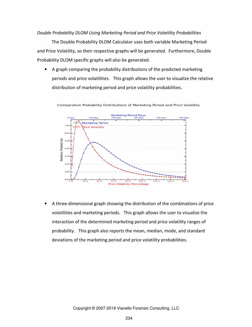
Copyright © 2007-2019 Vianello Forensic Consulting, LLC 234
Double Probability DLOM Using Marketing Period and Price Volatility Probabilities
The Double Probability DLOM Calculator uses both variable Marketing Period
and Price Volatility, so their respective graphs will be generated. Furthermore, Double
Probability DLOM specific graphs will also be generated.
• A graph comparing the probability distributions of the predicted marketing
periods and price volatilities. This graph allows the user to visualize the relative
distribution of marketing period and price volatility probabilities.
• A three-dimensional graph showing the distribution of the combinations of price
volatilities and marketing periods. This graph allows the user to visualize the
interaction of the determined marketing period and price volatility ranges of
probability. This graph also reports the mean, median, mode, and standard
deviations of the marketing period and price volatility probabilities.

Copyright © 2007-2019 Vianello Forensic Consulting, LLC 235
• A 2-dimensional matrix graph of the probability events color coded in red to
show events for which the raw Longstaff DLOM value exceeds 100%. This graph
displays and reports the percentage of marketing period and price volatility
combinations that result in raw Longstaff DLOM values greater than 100%. The
VFC Double Probability DLOM Calculator limits such events to 100% DLOM.
• A 3-dimensional graph of the probability events color coded in red to show
events for which the raw Longstaff DLOM values exceed 100%. This graph

Copyright © 2007-2019 Vianello Forensic Consulting, LLC 236
allows the user to visualize the overall influence of marketing period and price
volatility combinations that have been limited by the VFC DLOM Calculator®.
• A series of graphs that compare (a) the cumulative growth of probability
adjusted and value limited DLOM over time measured at the mean, median, and
mode of price volatility; and (b) the raw Longstaff DLOM value that would result
from applying the Longstaff formula for the particular marketing period without
adjusting for the probability of occurrence or limiting the calculated DLOM to
100%. Marketing periods resulting in greater than 100% DLOM for a fixed
volatility are shown in red if they occur.

Copyright © 2007-2019 Vianello Forensic Consulting, LLC 237

Copyright © 2007-2019 Vianello Forensic Consulting, LLC 238
•
• A series of graphs that compare (a) the cumulative growth of probability
adjusted and value limited DLOM over the predicted range of price volatility
measured at the mean, median, and mode of marketing period probabilities; and
(b) the raw Longstaff DLOM value that would result from applying the Longstaff
formula for the particular price volatility without adjusting for the probability of
occurrence or limiting the calculated DLOM to 100%. Price volatilities resulting
in greater than 100% DLOM for a fixed marketing period are shown in red if they
occur.

Copyright © 2007-2019 Vianello Forensic Consulting, LLC 239
• A graph comparing the distributions of DLOM based on the predicted marketing
period and price volatility trends. This graph allows the user to visualize the
different influences of marketing period and price volatility on the VFC
Probability-Based DLOM.

Copyright © 2007-2019 Vianello Forensic Consulting, LLC 240
•
• A three-dimensional graph showing the distribution of the VFC Probability-Based
DLOM. This graph allows the user to visualize how DLOM is influenced by the
combination of the range of marketing period and price volatility probabilities.

Copyright © 2007-2019 Vianello Forensic Consulting, LLC 241
• A three-dimensional graph showing cumulative growth of the double probability
distribution of DLOM.

Copyright ©
Limited Free Trial Mode
The current mode of the
page. All Calculators and Estimators
Free Trial” button to activate the trial mode.
During the trial mode users cannot change their Project and cannot use some
parts of the Marketing Period Inputs and Price Volatility tools. However,
mode users will not be charged any credits for using the
these free trials to get acquainted with how the
view the results they generate.
Click the “Exit Free Tria
free trial mode
Copyright © 2007-2019 Vianello Forensic Consulting, LLC 242
Limited Free Trial Mode
The current mode of the Calculator or Estimator is displayed at the top of the
Estimators have a free trial mode available. Click the “Explore
button to activate the trial mode.
During the trial mode users cannot change their Project and cannot use some
parts of the Marketing Period Inputs and Price Volatility tools. However, during trial
mode users will not be charged any credits for using the Calculators or Estimators
these free trials to get acquainted with how the Calculators and Estimators
view the results they generate.
lick the “Exit Free Trial” button located at the top of the screen to exit limited
is displayed at the top of the
the “Explore
During the trial mode users cannot change their Project and cannot use some
during trial
Estimators. Use
work and
to exit limited