E N A B L I N G P O LY H E D R A L O P T I M I Z AT I O N S I N L LV M

tobias christian grosser

Diploma Thesis

Programming GroupDepartment of Informatics and Mathematics

University of Passau

Supervisor: Prof. Christian Lengauer, Ph.D.Second reader: Priv. Doz. Dr. Martin Griebl

Tutor: Dr. Armin Größlinger

April 2011

Tobias Christian Grosser: Enabling polyhedral optimizations in LLVM, Diploma Thesis, ©April 2011

A B S T R A C T

Sustained growth in high performance computing and the availability of advanced mo-bile devices increase the use of computation intensive applications. To ensure fast execu-tion and consequently low power usage modern hardware provides multi-level caches,multiple cores, SIMD instructions or even dedicated vector accelerators. Taking advan-tage of those manually is difficult and often not possible in a portable way. Fortunately,advanced techniques that increase data-locality and parallelism with the help of poly-hedral abstractions are known to be effective in exploiting hardware capabilities. Yet,their automatic use is currently limited. They are mostly implemented in language spe-cific source-to-source compilers which can only optimize manually annotated code thatmatches a certain canonical structure. Furthermore, polyhedral optimizers often targetC or CUDA code, which limits efficient communication with compiler internals and canlead to missed optimization opportunities.

In this thesis we present Polly, a project to enable polyhedral optimizations in LLVM.LLVM is an infrastructure project used in compilers for a large set of different pro-gramming languages. It is built around a low-level intermediate representation (LLVM-IR) that allows language independent optimizations. We present how Polly can applypolyhedral transformations on this representation. This includes the detection of staticcontrol parts, their translation into a Z-polyhedra based representation, optimizationson this representation and finally, the generation of optimized LLVM-IR. We also de-fine an interface to connect external optimizers and show a novel approach to detectparallelism which is used to generate SIMD and OpenMP code. Finally, we show insome experiments how Polly can be used to automatically apply optimizations for datalocality and parallelism.

iii

A C K N O W L E D G M E N T S

I would like to thank the people who contributed to the development of Polly andcontinue to develop Polly with me. Hongbin Zheng worked on larger parts of the frontend, the general infrastructure and the test cases, Raghesh A worked on OpenMP codegeneration, and Andreas Simbürger helped with the connection to CLooG.

For my academic background I want to thank Albert Cohen, Martin Griebl, ArminGrößlinger, Sebastian Pop, Louis-Noël Pouchet, and Sven Verdoolaege, who largely af-fected this work. Those people raised my interest for polyhedral techniques, helped mewith my first steps and guided me during the last years. Today they are an invaluablesource of knowledge. Thank you for all the helpful discussions.

I would especially like to thank P. Sadayappan, who generously supported my workon Polly with a research scholarship at Ohio State (NSF 0811781 and 0926688), DirkBeyer, who supported the development of the RegionInfo analysis with several univer-sity projects and Christian Lengauer, who allowed me to work on Polly for my thesis.

v

C O N T E N T S

1 introduction 1

i background 5

2 llvm 7

2.1 Architecture . . . . . . . . . . . . . . . . . . . . . . . . . . . . . . . . . . . . . . 7

2.2 Intermediate Representation (LLVM-IR) . . . . . . . . . . . . . . . . . . . . . . 9

2.2.1 Types . . . . . . . . . . . . . . . . . . . . . . . . . . . . . . . . . . . . . . . . . 9

2.2.2 Instructions . . . . . . . . . . . . . . . . . . . . . . . . . . . . . . . . . . . . . 11

2.3 Analysis Passes . . . . . . . . . . . . . . . . . . . . . . . . . . . . . . . . . . . . 13

2.3.1 Dominator Tree . . . . . . . . . . . . . . . . . . . . . . . . . . . . . . . . . . . 14

2.3.2 Loop Information . . . . . . . . . . . . . . . . . . . . . . . . . . . . . . . . . . 15

2.3.3 Region Information . . . . . . . . . . . . . . . . . . . . . . . . . . . . . . . . . 16

2.3.4 Scalar Evolution . . . . . . . . . . . . . . . . . . . . . . . . . . . . . . . . . . . 18

2.3.5 Alias Analysis . . . . . . . . . . . . . . . . . . . . . . . . . . . . . . . . . . . . 20

2.4 Canonicalization . . . . . . . . . . . . . . . . . . . . . . . . . . . . . . . . . . . 21

2.4.1 Loop Canonicalization . . . . . . . . . . . . . . . . . . . . . . . . . . . . . . . 21

3 integer polyhedra 23

3.1 Integer Set . . . . . . . . . . . . . . . . . . . . . . . . . . . . . . . . . . . . . . . 23

3.2 Integer Map . . . . . . . . . . . . . . . . . . . . . . . . . . . . . . . . . . . . . . 25

3.3 Properties and Operations on Sets and Maps . . . . . . . . . . . . . . . . . . . 25

ii polly 27

4 architecture 29

4.1 How to Use Polly . . . . . . . . . . . . . . . . . . . . . . . . . . . . . . . . . . . 29

4.1.1 Polly’s LLVM-IR Passes . . . . . . . . . . . . . . . . . . . . . . . . . . . . . . 30

4.1.2 pollycc - A Convenient Polyhedral Compiler . . . . . . . . . . . . . . . . . . 30

5 llvm-ir to polyhedral description 33

5.1 What can be Translated? . . . . . . . . . . . . . . . . . . . . . . . . . . . . . . . 34

5.2 How is a SCoP Defined on LLVM-IR? . . . . . . . . . . . . . . . . . . . . . . . 35

5.3 The Polyhedral Representation of a SCoP . . . . . . . . . . . . . . . . . . . . . 37

5.4 How to Create the Polyhedral Representation from LLVM-IR . . . . . . . . . 39

5.5 How to Detect Maximal SCoPs . . . . . . . . . . . . . . . . . . . . . . . . . . . 40

5.6 Preparing Transformations . . . . . . . . . . . . . . . . . . . . . . . . . . . . . . 43

5.6.1 LLVM canonicalization passes . . . . . . . . . . . . . . . . . . . . . . . . . . 43

5.6.2 Create Independent Basic Blocks . . . . . . . . . . . . . . . . . . . . . . . . . 43

6 polyhedral optimizations 47

6.1 Transformations on the Polyhedral Representation . . . . . . . . . . . . . . . 47

6.2 External Optimizers - JSCoP . . . . . . . . . . . . . . . . . . . . . . . . . . . . . 52

6.3 Dependency Analysis . . . . . . . . . . . . . . . . . . . . . . . . . . . . . . . . 54

7 polyhedral description to llvm-ir 57

7.1 Generation of a Generic AST . . . . . . . . . . . . . . . . . . . . . . . . . . . . 57

vii

viii

7.2 Analyses on the Generic AST . . . . . . . . . . . . . . . . . . . . . . . . . . . . 57

7.2.1 Detection of Parallel Loops . . . . . . . . . . . . . . . . . . . . . . . . . . . . 59

7.2.2 The Stride of a Memory Access Relation . . . . . . . . . . . . . . . . . . . . 59

7.3 Generation of LLVM-IR . . . . . . . . . . . . . . . . . . . . . . . . . . . . . . . 61

7.3.1 Sequential Code Generation . . . . . . . . . . . . . . . . . . . . . . . . . . . . 62

7.3.2 OpenMP Code Generation . . . . . . . . . . . . . . . . . . . . . . . . . . . . 63

7.3.3 Vector Code Generation . . . . . . . . . . . . . . . . . . . . . . . . . . . . . . 63

iii experiments 69

8 matrix multiplication - vectorized 71

9 automatic optimization of the polybench benchmarks 75

9.1 The identity transformation . . . . . . . . . . . . . . . . . . . . . . . . . . . . . 75

9.2 Creating Optimized Sequential Code with Pluto . . . . . . . . . . . . . . . . . 76

9.3 Creating Optimized Parallel Code with Pluto . . . . . . . . . . . . . . . . . . . 77

10 conclusion 79

iv appendix 81

List of Figures 83

List of Tables 85

List of Listings 86

List of Acronyms 87

references 89

1I N T R O D U C T I O N

motivation

Computation intensive applications are prevalent on high performance clusters andwork stations, but gain also importance on mobile devices and web clients. There, theincreased use of features like object and gesture recognition [45, 53], computationalphotography [32, 55] and augmented reality [52] yields to a steadily growing numberof computation intensive applications. Further increases can be expected due to theintegration of high quality cameras and other advanced input devices. Hence, efficientprogram execution is not only relevant on high performance clusters, but also on mobiledevices. Efficiency is here crucial for instant user feedback and long battery life.

Modern hardware provides many possibilities to execute a program efficiently. Mul-tiple levels of caches help to exploit data-locality and there are various ways to takeadvantage of parallelism. Short vector instruction sets such as Intel SSE and AVX, IBMAltiVec as well as ARM NEON can be used for fine grained parallelism. Dedicated vec-tor accelerators or GPUs supporting general purpose computing may be used for mas-sively parallel tasks. On platforms like IBM Cell, Intel SandyBridge and AMD Fusionsimilar accelerators are available tightly integrated with general purpose CPUs. Finally,an increasing number of computation cores exists even on ultra mobile platforms. Theeffective use of all available resources is important for high efficiency. Consequently,well optimized programs are necessary.

Traditionally, such optimizations are performed by translating performance criticalparts of a software system into a low-level language like C or C++ and by optimizingthem manually. This is a difficult task as most compilers support basic loop transforma-tions as well as inner and outer loop vectorization, but as soon as complex transforma-tions are necessary to ensure the required data-locality or to expose the various kindsof parallelism, little compiler support is available. The problem is further complicatedif hints are needed by the compiler, OpenMP parallel loops need to be annotated oraccelerators should be used. As a result, only domain experts are able to perform suchoptimizations effectively.

Even if they succeed, there remain other problems. First of all, such optimizationsare extremely platform dependent and often not even portable between different mi-croarchitectures. Consequently, programs need to be optimized for every target archi-tecture separately. This becomes increasingly problematic, as today an application maytarget at the same time ARM based iPhones, Atom and AMD Fusion based netbooksas well as a large number of desktop processors, all equipped with a variety of differ-ent graphic and vector accelerators. Furthermore, manual optimizations are often even

1

2

impossible. High level language features like the C++ standard template library blockmany optimizations. Languages such as Java, Python and JavaScript provide no sup-port for portable low level optimizations. Even programs compiled for Google NativeClient [56], a framework for portable, calculation intensive web applications, will faceportability issues, if advanced hardware features are used. In brief, manual optimiza-tions are complex, non-portable and often even impossible.

Fortunately, powerful algorithms are available to optimize computation intensiveprograms automatically. Wilson et al. [54] implemented automatic parallelization anddata-locality optimizations based on unimodular transformations in the SUIF compiler,Feautrier [21] developed an algorithm to calculate a parallel execution order fromscratch and Griebl and Lengauer [24] developed LooPo, a complete infrastructure tocompare different polyhedral algorithms and concepts. Furthermore, Bondhugula et al.[13] created Pluto, an advanced data-locality optimizer that simultaneously exposesthread and SIMD level parallelism. There are also methods to offload calculations toaccelerators [10, 9] and even techniques to synthesize high-performance hardware [43].All these techniques are part of a large set of advanced optimization algorithms builton polyhedral concepts.

However, the use of these advanced algorithms is currently limited. Most of them areimplemented in source to source compilers, which use language specific front ends toextract relevant code regions. This often requires the source code of these regions to bein a canonical form and to not contain any pointer arithmetic or higher level languageconstructs such as C++ iterators. Furthermore, the manual annotation of code that is safeto optimize is often necessary, as even tools limited to a restricted subset of C commonlyignore effects of implicit type casts, integer wrapping or aliasing. Another problemis that most implementations target C code and subsequently pass it to a compiler.The limited integration blocks effective communication between polyhedral tools andcompiler internal optimizations. As a result, influencing performance related decisionsof the compiler is difficult and the resulting programs often suffers from poor registerallocation, missed vectorization opportunities or similar problems.

We can conclude that a large number of computation intensive programs exist, thatneed to be optimized automatically to be executed efficiently on current hardware. Ex-isting compilers have difficulties with the required complex transformations, but thereis a set of advanced polyhedral techniques that are proven to be effective. Yet, they missintegration in a production compiler to have significant impact.

contributions

With Polly1 we present a polyhedral infrastructure for LLVM that supports fully au-tomatic transformation of existing programs. Polly detects and extracts relevant coderegions without any human interaction. Since Polly optimizes the LLVM intermediaterepresentation (LLVM-IR), it is programming language independent and transparentlysupports constructs like C++ iterators, pointer arithmetic or goto based loops. It is builtaround an advanced polyhedral library [50] that supports existentially quantified vari-ables and provides a state-of-the-art dependency analysis. Due to a simple file interfaceit is easily possible to apply transformations manually or to use an external optimizer.

1 The word Polly is a combination of Polyhedral and LLVM. It is pronounced like Polly, the parrot.

3

We use this interface to integrate Pluto [13], a modern data locality optimizer and par-allelizer. Thanks to integrated SIMD and OpenMP code generation, Polly automaticallytakes advantage of existing and newly exposed parallelism.

This thesis is organized as follows. In Chapter 2 and 3 we give some backgroundon LLVM and Z-polyhedra. Then we describe the concepts and techniques developedwithin Polly. We start in Chapter 4 with presenting the architecture of Polly and thetools developed to use it. Next, we explain in Chapter 5 the detection of relevant coderegions in LLVM-IR and their translation into a polyhedral description. We also definethe description itself. In Chapter 6 we present an advanced dependency analysis onthis representation and we show how optimizations on it are performed. In this chapterwe also define an exchange format to connect external optimizers. In Chapter 7 wedescribe how we regenerate LLVM-IR and how to automatically create OpenMP and SIMDparallel code. After the concepts developed within Polly are explained, we show someexperiments in Chapters 8 and 9, that help to understand the impact of our currentimplementation. Finally, we conclude in Chapter 10.

Part I

B A C K G R O U N D

2L LV M

The Low Level Virtual Machine (LLVM) is a compiler framework described in Lattnerand Adve [31]. It is built around the LLVM Intermediate Representation (LLVM-IR) andcomes with a large variety of analysis and transformation passes. The whole frameworkwas especially designed to optimize a program throughout its lifetime, which means atcompile time, link time and even run time. Furthermore, LLVM includes back endsfor static and just-in-time code generation for architectures like x86-32, x86-64, ARM orPowerPC.

LLVM based compilers exist for a variety of programming languages. There are staticcompilers like LLVM clang or the GCC based compilers dragonegg [1] and llvm-gcc.clang compiles C, C++ and Objective-C whereas dragonegg and llvm-gcc additionallysupport FORTRAN, Ada and Go. Furthermore, there are compilers for dynamic lan-guages like Python [6], Ruby [5] and Lua [3] and for bytecode based virtual machineslike Java [2] and .NET [47]. With the Glasgow Haskell Compiler (GHC) even a compilerfor an all functional language includes LLVM based code generation [46]. LLVM is alsoused in areas like graphics shader optimization, GPGPU computing or for the AMD [33],Apple and Nvidia OpenCL compilers [34]. There exist even a notable number of projectsto use LLVM for High Level Synthesis (HLS) [51, 14, 57, 40]

2.1 architecture

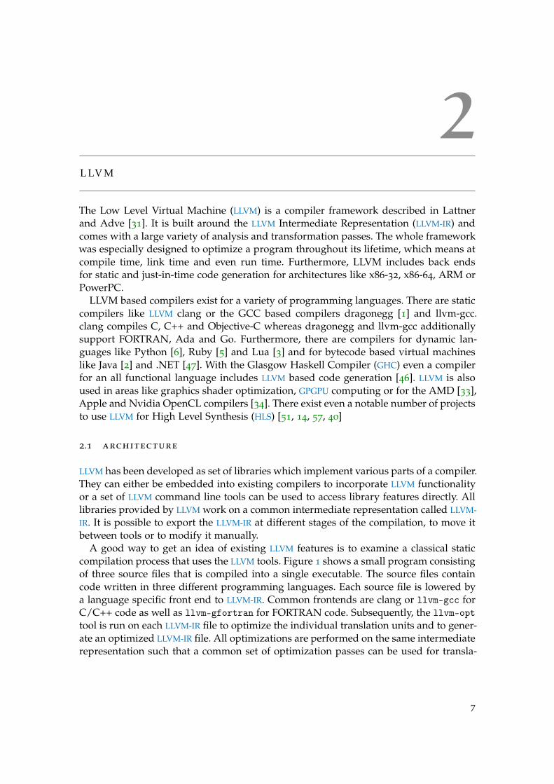
LLVM has been developed as set of libraries which implement various parts of a compiler.They can either be embedded into existing compilers to incorporate LLVM functionalityor a set of LLVM command line tools can be used to access library features directly. Alllibraries provided by LLVM work on a common intermediate representation called LLVM-IR. It is possible to export the LLVM-IR at different stages of the compilation, to move itbetween tools or to modify it manually.

A good way to get an idea of existing LLVM features is to examine a classical staticcompilation process that uses the LLVM tools. Figure 1 shows a small program consistingof three source files that is compiled into a single executable. The source files containcode written in three different programming languages. Each source file is lowered bya language specific front end to LLVM-IR. Common frontends are clang or llvm-gcc forC/C++ code as well as llvm-gfortran for FORTRAN code. Subsequently, the llvm-opttool is run on each LLVM-IR file to optimize the individual translation units and to gener-ate an optimized LLVM-IR file. All optimizations are performed on the same intermediaterepresentation such that a common set of optimization passes can be used for transla-

7

8

main.cppmoduleA.f90moduleB.c

main.llmoduleA.llmoduleB.ll

main.opt.llmoduleA.opt.llmoduleB.opt.ll

program.ll

program.opt.ll program.s program.o program.exeprogram.ll

clangllvm-gcc

llvm-gfortran

Frontends

llvm-opt

Optimizerllvm-link

Linker

llvm-opt

Optimizerllvm-mc

Assemblerllvm-llc

Target Code Generator

ld

SystemLinker

Figure 1: Static compilation using the llvm toolchain

tion units created from different programming languages. The optimizers can be run asset of standard optimizations passes or as individually selected passes. This is especiallyhelpful if e.g. only dead code elimination should be performed or the LLVM-IR shouldbe canonicalized in a certain way.

After the individual parts have been optimized llvm-link combines them to a singlemodule, which can be optimized again by llvm-opt. At this point specific link timeoptimizations are scheduled that for instance mark all functions as internal. In additiona set of standard optimizations is run, as they may apply again after the link timespecific optimizations. As modules created from different programming languages arelinked together, optimizations can cross language borders without difficulty. Therefore,it is possible to inline a function written in FORTRAN into some code written in C++.

Up to this point all transformations can be performed target agnostic. The first trans-formation that cannot is the lowering from LLVM-IR to target specific machine code.However, even at this stage LLVM uses a target independent code generation infras-tructure that provides generic support for instruction selection or register allocation.The target code generators for the different supported architectures are based on thisgeneric infrastructure and can be specialized by target specific optimizers. Instructionselection is in charge of selecting the best machine code instructions to implement a setof LLVM-IR instructions. Machine specific aligned or unaligned load instructions are e.g.selected to implement a generic load depending on the alignment information LLVM-IRprovides. A sequence of an add and a multiply instruction can be lowered to a ma-chine specific fused multiply add. In addition arbitrary width vector types, as providedby LLVM-IR, are lowered to machine instructions that work on vectors of target specificwidth.

llvm-llc is the tool that creates target assembler code from LLVM-IR. As LLVM codegeneration uses a generic machine code infrastructure, it is also possible to directly emitobject files bypassing any assembler. The same infrastructure is used in the llvm-mc

9

tool, which provides an assembler, a disassembler as well as ways to obtain informationlike the encoding of machine instructions. The machine code infrastructure can also beused by the target independent optimization passes of LLVM which obviously can taketarget specific information into account. Therefore, unrolling or inlining decisions canbe taken based on the real instruction encoding instead of some rough estimates. Thisis especially important for modern CISC architectures.

Another area where the machine code infrastructure is very useful is the just in timeinfrastructure of LLVM. Instead of creating static object files LLVM supports just-in-timecode generation such that machine code is directly emitted to memory and executedright ahead. As the LLVM just in time compiler uses LLVM-IR to describe the programs alloptimization passes available for static compilation can be applied during just-in-timecompilation. It is conceptually even possible to reoptimize with different parameters e.g.to especially optimize hot functions or to take advantage of knowledge obtained duringthe execution of the program.

Overall, LLVM provides a consistent infrastructure for the whole compilation processthat is used in many important compilers. As all compilers target LLVM-IR as commonintermediate representation LLVM is a great platform to write programming languageand target independent optimizations.

2.2 intermediate representation (llvm-ir)

LLVM uses a common intermediate representation called LLVM-IR throughout the wholecompilation process. All compilers that use LLVM as optimizer and code generatorlower their input language to LLVM-IR. LLVM-IR is a typed, target agnostic, assemblerlike language for a register machine with an infinite amount of virtual registers. Eachregister can only be written once, such that register operations are in Static SingleAssignment (SSA) form. As LLVM is a load/store architecture, values are transfered be-tween memory and registers via explicit load or store operations.

There exist three representations of LLVM-IR. First there is the in-memory representa-tion used inside the library, then there is the on-disk bytecode representation (.bc files)used e.g. for caching the output of a just-in-time compiler and finally there is the humanreadable assembly language representation (.ll files). All three are equivalent in termsof expressiveness. In this thesis the human readable representation is used.

This section describes the subset of LLVM-IR relevant for Polly and highlights impor-tant aspects. A full definition is available from Lattner [30].

2.2.1 Types

LLVM-IR is strongly typed, which means every register, function parameter, functionreturn value or instruction has an associated type. There exist no implicit type casts. Theoperands provided to functions or instructions must always match the required types.The only way to change the type of a value is an explicit cast. Code without explicitcasts in the LLVM-IR is always type safe. However, casts may be needed to express thetype systems of more abstract languages. As a result types in LLVM-IR correspond notnecessarily to the ones that exist in the language from which the LLVM-IR is generated.

10

The types can be divided into two major groups: primitive types and derived types.Primitive types are the basic types. Derived types are constructed by recursively com-posing such basic types.

There are three kinds of primitive types relevant for Polly: the integer types, thefloating point types and the label type. LLVM-IR supports integer types of arbitrary butfixed bit width called iX, where X is the bit width of the integer. All optimizations andanalyses are implemented on these arbitrary width integers. As not all targets haverobust code generation for large bit widths, the use of types beyond i128 is limited. Incontrast to C integer types in LLVM-IR do not define signedness. The interpretation ofthe integer values depends on the instruction that uses them. For further informationsee Section 2.2.2. LLVM-IR also defines floating point types for single, double as well asquadruple precision. All available floating point types are signed. Finally, there is thelabel type that represents locations in the source code which can be used as a target forbranch and switch instructions. Common primitive types are :

i1 ; Boolean valuei8 ; C (unsigned) chari32 ; 32 bit (unsigned) integeri64 ; 64 bit (unsigned) integer

float ; Single precision floating point valuedouble ; Double precision floating point valuex86_fp80 ; X87 80bit floating point valuefp128 ; Quadruple precision floating point value

label ; The label of a basic block

There are three kinds of derived types interesting to Polly: the pointer types, thearray types and the vector types. A pointer type specifies the location of an object inmemory. An array type describes a set of elements arranged sequentially in memory.It has always a fixed size known at compile time. There are no variable sized multi-dimensional arrays in LLVM-IR. Variable sized arrays need to be expressed based onpointers and pointer arithmetic. A vector type represents a vector of elements. It isdefined by the number of contained elements and their common primitive type. Vectortypes are used as operands in SIMD operations. They can have arbitrary width and willbe lowered by the target back ends to the machine vector width. As this lowering isdone in the target code generation, no further LLVM-IR optimizations are applied. As aresult, code generation for vectors that are notably larger than the machine vector widthis not optimal. Common derived types are:

float * ; A pointer to a float<4 x float> * ; A pointer to a vector of four floats

[20 x float] ; An array of 20 float elements[5 x [3 x double]] ; An array that consists of five arrays

; each containing three doubles

11

<4 x float> ; A vector of four floats<16 x i8> ; A vector of 16 C chars

All types mentioned in this section are also first class types. First class types can becreated by LLVM-IR instructions and can be passed as function parameter or returned bya function.

2.2.2 Instructions

LLVM-IR has on purpose a very limited set of instructions to describe a program. It onlyrepresents common operations. Specific machine instructions are created when LLVM-IRis lowered in the back end. The set of LLVM-IR instructions needed to understand Pollyis even smaller. In this section we will have a look at instructions for computations,vector management, type conversion, memory management and finally control flowinstructions.

First we look at computational instructions that perform a side effect free operationon a set of operands. Operands are in this case either virtual registers or constant val-ues. There exist three groups of computational instructions: Binary instructions, bitwiseinstructions and comparison instructions. Binary instructions as well as comparison in-structions are defined for both floating point and integer types, whereas bitwise instruc-tions are only defined on integer types. Furthermore, there exist corresponding vectorversions of all instructions, which take integer or floating point vector types as operandsand perform the same operation as the non-vector instruction, but elementwise on thewhole vector. The complete set of binary instructions consists of addition, subtraction,multiplication, division and modulo operation. For integer types there exist signed andunsigned versions of the division and the modulo operation. This is not needed forfloating point types, as they are always signed. Integer types are interpreted followingthe two’s complement representation with defined overflow semantics for addition, sub-traction and multiplication Hence, no special signed or unsigned versions are neededfor those instructions. Various bitwise instructions allow different kinds of shifts as wellas the boolean operations and, or and xor. Finally there are comparison instructions,which support a common set of comparisons. Some computational instructions are:

%result = add i32 %firstOp, %secondOp%resultF = fmul float %firstFOp, %secondFOp%resultOr = or i8 %firstBitSet, %secondBitSet%vectorDiv = fdiv <8 x double> %vectorOne, %vectorTwo%vectorCmp = icmp eq <8 x i16> %intVectorOne, %intVectorTwo

The instructions just described only work on virtual registers. Hence it is necessary toload values from memory into registers before the instructions are executed and to storethe results of a calculation from a register back to memory. The only instructions neededfor this are called load and store and move a value from a register to an address inmemory or the other way around. There are two ways to obtain the address of an objectin memory. Either by allocating a new one on the stack using alloca or by using systemprovided functions for memory allocation like malloc to allocate memory elsewhere.LLVM provides a third way called getelementptr which is an instruction that takes the

12

start address of an array and returns the address of an element at a certain offset. Thisinstruction is used for type safe memory address calculations. To calculate the offset, thetype of the elements in the array needs to be provided. As LLVM does not provide typesfor variable sized arrays only arrays that contain fixed size elements can be modeled thisway. Variable sized arrays need to be implemented by manually calculating the relevantmemory offsets. Another information available for these memory instructions is thealignment of the memory accessed. If alignment information is provided, the targetcode generator can use more efficient aligned machine operations. Possible memoryoperations are:

%memoryAddress = alloca float, align 4store float 3.0, float* %memoryAddress, align 4%register = load float* %memoryAddress, align 4%vectorPtr alloca = <4 x float>, align 32%vectorLoad = load <4 x float> %vectorPtr, align 32

With the features so far, it is possible to do pure scalar calculations and pure vectorcalculations. However it is often needed to build a vector from a set of scalars or toextract a scalar from a vector. Therefore LLVM provides the instructions insertelementand extractelement. Furthermore, a generic shuffle instruction is provided that takestwo vectors and combines their content based on a shuffle mask. These are the onlyvector specific instructions. All other operations on vectors are provided by genericinstructions. Some vector specific operations are:

%resultVec1 = insertelement <4 x float> %vec, float 5.0, i32 0%resultVec2 = insertelement <4 x float> %resultVec1, float 3.2, i32 1%resultVec3 = insertelement <4 x float> %resultVec2, float 8.4, i32 1%shuffleResult = shufflevector <4 x float> %resultVec2, <4 x float> %resultVec3,

<3 x i32> <i32 0, i32 1, i32 5>%scalar = extractelement <4 x float> %resultVec3, i32 1

; %shuffelResult is <5.0, 3.2, 8.4>; %scalar is 8.4

To allow calculations between types of different sizes or between floating point andinteger types LLVM provides a set of cast and conversion instructions that provide typeextensions and truncation for both integer and floating point types, with special signedand zero extension methods available for integer types. Furthermore, signed and un-signed versions for float to integer conversion are provided. Finally, a bitcast instructionis available to reinterpret a set of values without modifying the actual memory content.This can for instance be used to change a pointer to a scalar into a pointer to a vector.Common conversion instructions are:

%smallint = trunc i32 %largeint to %i16%hugeint = zext i32 %largeint to %i64%float = fptrunc double 42.0 to float

%vectorPtr = bitcast i32* %scalarPtr to <2 x i32>*%register = load <2 x i32>* %vectorPtr

13

So far only sequentially ordered instructions have been discussed. A set of such in-structions that does not include any branch is called a basic block. Each basic block islabeled with a name. To create constructs like loops or conditional control flow thesebasic blocks are connected by so-called terminator instructions that direct the controlflow from one basic block to another. Terminator instructions are required as last in-struction of a basic block and are only allowed at this place. The most common ones arebranch, switch and ret. The first describes either an unconditional branch to a singlelabel or a conditional branch to two labels. The switch is a generic branch instructionto a numbered set of labels, where the target of the branch is provided by an integervalue. And finally there is the ret instruction to terminate the control flow in a functionand to return a value. As terminator instructions are required and the targets can onlybe known labels, an explicit Control Flow Graph (CFG) is created. Another control flowinstruction is the phi instruction, which merges values defined in the predecessors of abasic block into a single register value. The following code shows some examples:

start:%condition = icmp eq i32 5, 10 ; 5 == 10 is Falsebr %condition, label %left, label %right ; Branch to %right

left:%plusOne = add i32 0, i32 1 ; 0 + 1 (not executed)br label %join ; Branch to %join (not executed)

right:%minusOne = sub i32 0, i32 1 ; 0 - 1br label %join ; Branch to %join

merge:%joinedValue = phi i32 [ %plusOne, %left], ; Copy value from %minusOne

[ %minusOne, %right]ret i32 %joinedValue ; return %joinedValue

Overall, LLVM-IR is a small language that was shown to be expressive enough to rep-resent a wide range of programming languages and preserves enough information toapply sophisticated analysis and transformations. The small size of the language sim-plifies analysis and transformation on it and allows them to cover the whole languageeasily. Through the consistent integration of vector types it is furthermore a solid plat-form for machine independent vectorization.

2.3 analysis passes

As LLVM-IR is a relatively low-level program representation, information about higherlevel structures or global program state is in general not readily available. Neverthelessit is often possible to analyze LLVM-IR and to derive the information needed. This isfacilitated as LLVM already provides a set of sophisticated analysis passes [4]. We willpresent the ones used by Polly. As an example we use the following piece of code andits CFG representation as shown in Figure 2.

void foo() {int i, a, b;

14

1:int i, a, b

i = 0

2:if (i != 100)

T F

3:a = 4if (i == a)

T F

7:return

4:b = 5

5:b = 8

6:i++

Figure 2: CFG of the example program

for (i = 0; i != 100; i++) {a = 3;

if (i == a)b = 5;

elseb = 8;

}}

2.3.1 Dominator Tree

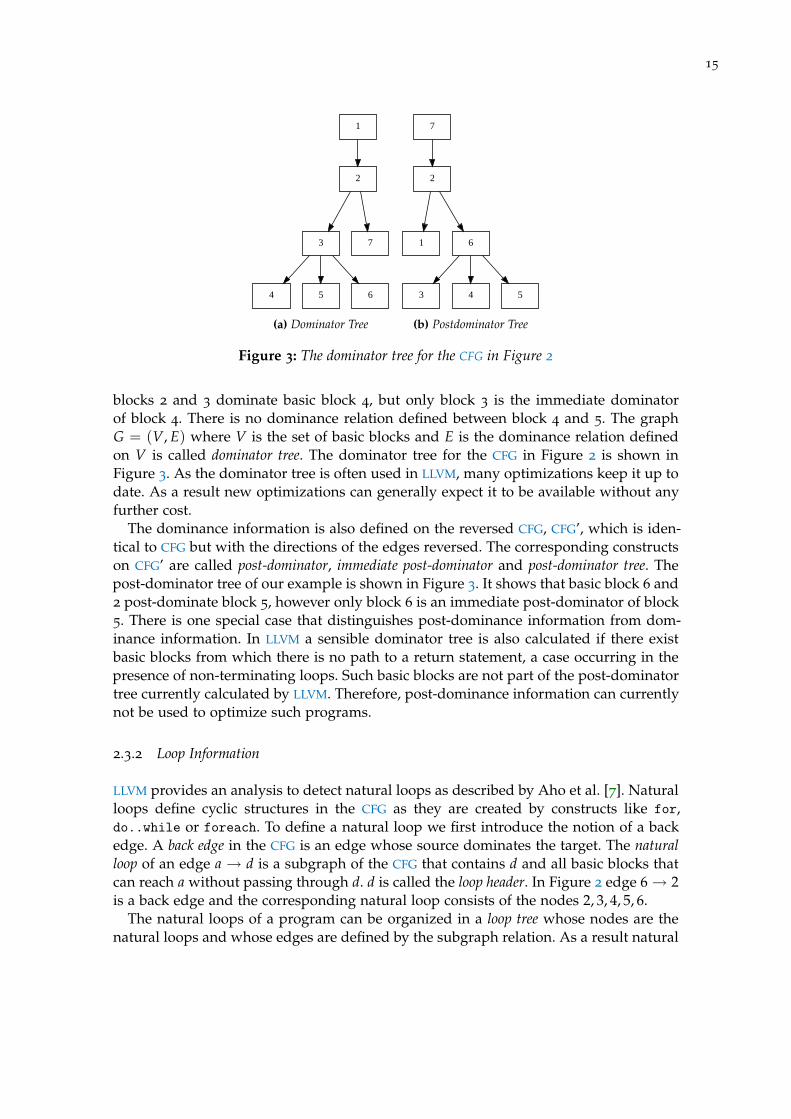
A commonly used analysis in LLVM is the dominance information1. It describes a rela-tion between the different basic blocks in the CFG. Prosser [38], who developed the ideaof a dominance information, introduced it with the following words:

“We say [block] i dominates [block] j if every path (leading from inputto output through the [CFG]) which passes through [block] j must also passthrough [block] i.”

i is called the dominator of j. It is called the immediate dominator of j, if there existsno other basic block that is dominated by i and that also dominates j. In Figure 2 basic

1 Section adapted from ’The refined program structure tree’ (Tobias Grosser), the description of a projectdeveloped in the class ’Softwareanalyse’ 09/10 with Dirk Beyer

15

1

2

3

7

4 5 6

(a) Dominator Tree

1

2

6

7

3 4 5

(b) Postdominator Tree

Figure 3: The dominator tree for the CFG in Figure 2

blocks 2 and 3 dominate basic block 4, but only block 3 is the immediate dominatorof block 4. There is no dominance relation defined between block 4 and 5. The graphG = (V, E) where V is the set of basic blocks and E is the dominance relation definedon V is called dominator tree. The dominator tree for the CFG in Figure 2 is shown inFigure 3. As the dominator tree is often used in LLVM, many optimizations keep it up todate. As a result new optimizations can generally expect it to be available without anyfurther cost.

The dominance information is also defined on the reversed CFG, CFG’, which is iden-tical to CFG but with the directions of the edges reversed. The corresponding constructson CFG’ are called post-dominator, immediate post-dominator and post-dominator tree. Thepost-dominator tree of our example is shown in Figure 3. It shows that basic block 6 and2 post-dominate block 5, however only block 6 is an immediate post-dominator of block5. There is one special case that distinguishes post-dominance information from dom-inance information. In LLVM a sensible dominator tree is also calculated if there existbasic blocks from which there is no path to a return statement, a case occurring in thepresence of non-terminating loops. Such basic blocks are not part of the post-dominatortree currently calculated by LLVM. Therefore, post-dominance information can currentlynot be used to optimize such programs.

2.3.2 Loop Information

LLVM provides an analysis to detect natural loops as described by Aho et al. [7]. Naturalloops define cyclic structures in the CFG as they are created by constructs like for,do..while or foreach. To define a natural loop we first introduce the notion of a backedge. A back edge in the CFG is an edge whose source dominates the target. The naturalloop of an edge a → d is a subgraph of the CFG that contains d and all basic blocks thatcan reach a without passing through d. d is called the loop header. In Figure 2 edge 6→ 2is a back edge and the corresponding natural loop consists of the nodes 2, 3, 4, 5, 6.

The natural loops of a program can be organized in a loop tree whose nodes are thenatural loops and whose edges are defined by the subgraph relation. As a result natural

16

int i, a, b i = 0

if (i != 100)

T F

a =4if (i == a)

T F

entry

return

b = 5 b = 8

i++

exit

Figure 4: A simple Region

loop L1 is a child of a natural loop L2 , if the basic blocks in L1 are also basic blocks inL2.

Furthermore, LLVM detects certain special forms of natural loops. A natural loop hasa preheader if there is a single basic block from which edges enter the loop. There existsa preheader of a loop, if there is a single basic block from which edges lead to the loopheader.

2.3.3 Region Information

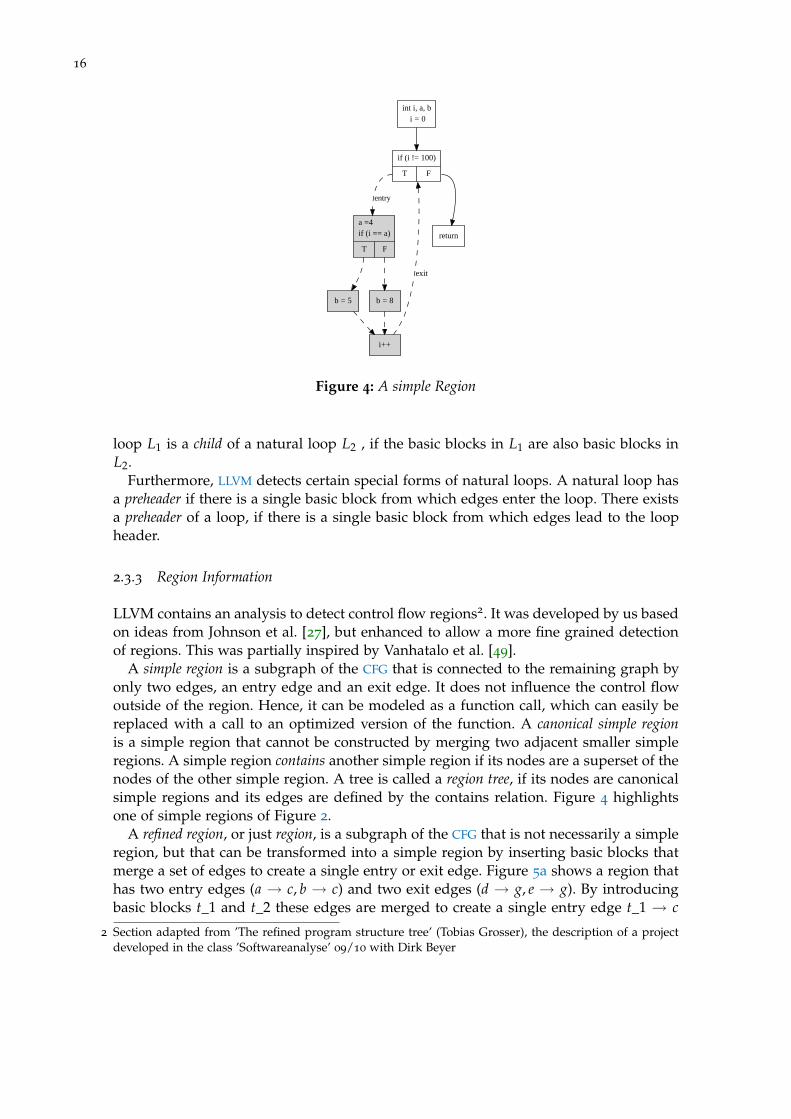
LLVM contains an analysis to detect control flow regions2. It was developed by us basedon ideas from Johnson et al. [27], but enhanced to allow a more fine grained detectionof regions. This was partially inspired by Vanhatalo et al. [49].

A simple region is a subgraph of the CFG that is connected to the remaining graph byonly two edges, an entry edge and an exit edge. It does not influence the control flowoutside of the region. Hence, it can be modeled as a function call, which can easily bereplaced with a call to an optimized version of the function. A canonical simple regionis a simple region that cannot be constructed by merging two adjacent smaller simpleregions. A simple region contains another simple region if its nodes are a superset of thenodes of the other simple region. A tree is called a region tree, if its nodes are canonicalsimple regions and its edges are defined by the contains relation. Figure 4 highlightsone of simple regions of Figure 2.

A refined region, or just region, is a subgraph of the CFG that is not necessarily a simpleregion, but that can be transformed into a simple region by inserting basic blocks thatmerge a set of edges to create a single entry or exit edge. Figure 5a shows a region thathas two entry edges (a → c, b → c) and two exit edges (d → g, e → g). By introducingbasic blocks t_1 and t_2 these edges are merged to create a single entry edge t_1 → c

2 Section adapted from ’The refined program structure tree’ (Tobias Grosser), the description of a projectdeveloped in the class ’Softwareanalyse’ 09/10 with Dirk Beyer

17

a

c

T F

entry

g

b

entry

d e

exit exit

(a) Refined region

a

t_1

g

b

c

T F

entry

d e

t_2

exit

(b) After transformation

Figure 5: Transform a refined region to a simple region

a

hg

i j

k

e

lb

d

f

c

Figure 6: Simple (solid border) and refined (dashed border) regions in a CFG.

18

and a single exit edge t_2 → g. Figure 5b shows the newly created simple region. Aregion is canonical if it cannot be created by merging two adjacent regions. We alsodefine a contains relation for refined regions following the definition for simple regions.Finally we define a refined region tree, also called refined program structure tree, as tree ofrefined regions connected by the contains relation.

Figure 6 shows a larger CFG that contains a set of different regions. Simple regionsare marked with solid borders whereas refined

2.3.4 Scalar Evolution

The scalar evolution analysis calculates for every integer register a closed form expres-sion describing its value during the execution of a program. This expression is calledthe scalar evolution of the register. It is used to abstract away the individual instructionsthat lead to the value of a register and to focus on the overall calculation. Scalar evolu-tion simplifies analysis and optimizations. It is for example used to eliminate redundantinstructions by comparing the scalar evolution of two registers and by eliminating oneif their scalar evolutions are identical.

The analysis implemented in LLVM is based on the work of Bachmann et al. [8]on chains of recurrences and the adaption of those to compilers and induction variableanalysis as described in various papers [58, 19, 37]. However, it is adapted and extendedto fit the needs of the LLVM framework. One notable extension is the modeling ofinteger wrapping in the expressions of the scalar evolution.

2.3.4.1 The elements of a scalar evolution

A scalar evolution expression is constructed recursively from the elements in Figure 7.There are two base elements and a larger set of inductively defined elements. The baseelements are the integer constant and the unknown value. An integer constant representsan integer known at compiler time whereas an unknown value represents an integerunknown at compile time. There are different kind of unknown values. The first iscalled undef and is used if a value is undefined in LLVM-IR and as a result will alsobe undefined during execution. The next is called %parameter and represents an integerthat is unknown at compile time, but known at execution time. Parameters appearfor example if a register is initialized through function parameters or by a load frommemory. Finally there exist unknown values to represent target specific constants in atarget independent way. These are SizeOf, AlignOf and OffSetOf which represent thesize of types, the alignment of types and the offset of elements in a structure.

The recursively defined elements of a scalar evolution can be grouped in unary castoperations, binary operations, n-ary operations and add recurrences. There exist threeunary cast operations to change the type and therefore the bit width of the value rep-resented. The trunk operation reduces the bit width and zext or sext increase the bitwidth by applying zero or sign extension. There is one binary operation, the unsigneddivision /u and there are the n-ary operations addition +, multiplication *, signed max-imum smax and unsigned maximum umax. All operations mentioned follow modulointeger arithmetics as defined for LLVM integer types.

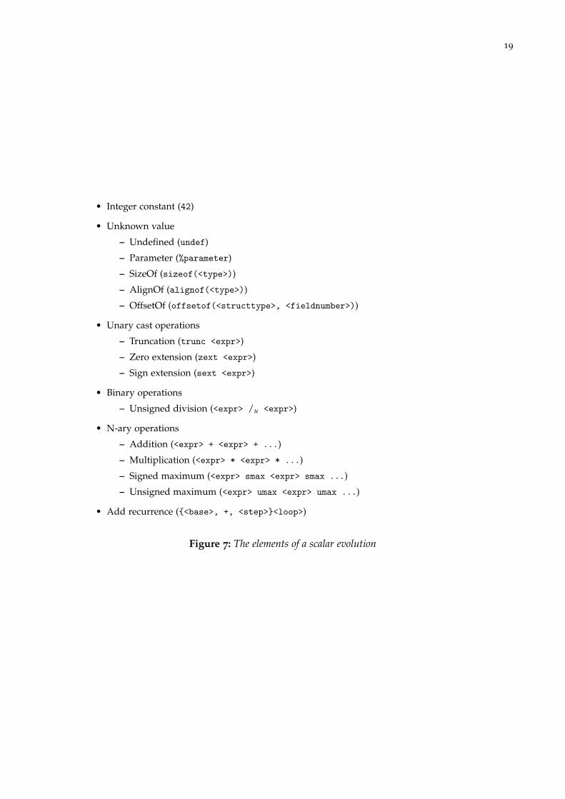
19

• Integer constant (42)

• Unknown value

– Undefined (undef)

– Parameter (%parameter)

– SizeOf (sizeof(<type>))

– AlignOf (alignof(<type>))

– OffsetOf (offsetof(<structtype>, <fieldnumber>))

• Unary cast operations

– Truncation (trunc <expr>)

– Zero extension (zext <expr>)

– Sign extension (sext <expr>)

• Binary operations

– Unsigned division (<expr> /u <expr>)

• N-ary operations

– Addition (<expr> + <expr> + ...)

– Multiplication (<expr> * <expr> * ...)

– Signed maximum (<expr> smax <expr> smax ...)

– Unsigned maximum (<expr> umax <expr> umax ...)

• Add recurrence ({<base>, +, <step>}<loop>)

Figure 7: The elements of a scalar evolution

20

Finally, there are add recurrences. Add recurrences represent expressions that changeduring the evaluation of a loop. They have the format {<base>, +, <step>}. The baseof an add recurrence defines its value at loop iteration zero and the step of an add recur-rence defines the values added on every subsequent loop iteration. An add recurrencerepresents an affine linear expression if its step is a constant expression not containingany further add recurrences. It represents a higher order polynomial function, if thestep is a non-constant expression. In general the maximal degree of a polynomial thatcan be expressed is limited by the nesting depth of the add recurrences.

2.3.4.2 Code that can be analyzed

The scalar evolution analysis in LLVM can analyze code that uses common integer arith-metic like addition, subtraction, multiplication, unsigned division. Furthermore, it sup-ports truncation, sign extension and zero extension and is able to recognize commonarithmetic idioms expressed by bitwise binary instructions or the different shift instruc-tions. Minimum and maximum constructs expressed with conditional instructions arealso commonly recovered. Loop variant expressions, which arise through the use of Φ-nodes, are detected for loops with a single entry edge and a single back edge. Finally,scalar evolution can analyze pointer arithmetic like it analyzes integer arithmetic.

Overall, scalar evolution is capable to derive closed form expressions for many ofthe integer variables in common programs. It is used in several important LLVM passeslike redundant induction variable elimination, loop canonicalization or loop strengthreduction. Hence it is as established in LLVM as more widely known analysis like thedominator information.

2.3.5 Alias Analysis

LLVM provides a sophisticated alias analysis infrastructure to calculate information onthe relation between different memory references. It consists of several alias analysispasses that can be combined to increase the precision of the overall analysis. Each passclassifies the relation between two memory accesses as either no alias, may alias, partialalias, or must alias. No alias signifies that two accesses will not touch the same memory,partial alias means the memory ranges accessed are known to partially overlap, and mustalias means the accessed memory is identical. In case no information about the relationbetween the memory accesses can be derived may alias is returned.

The different alias analysis passes available in LLVM are basic alias analysis, scalarevolution alias analysis and type based alias analysis. Basic alias analysis is the primaryalias analysis implementation in LLVM and provides stateless alias analysis information.It knows for example that two different globals cannot alias. The scalar evolution aliasanalysis is specialized on loop structures and derives information about possible alias-ing of memory references by comparing the scalar evolution expression of two loopvariant memory references. Finally, there is type based alias analysis. This analysis re-quires additional type information from a higher level type system. As a strict high-leveltype system can enforce that two pointers of different types do not point to the samememory, information about possible aliasing that is not available by only analyzing,LLVM-IR can be derived.

21

2.4 canonicalization

There are often numerous ways to represent a calculation in a program. To be able toapply an analysis or transformation on all of them, it needs to be written in a verygeneric way. This yields to complex code as many special cases need to be taken intoaccount and often even the complex code is often not generic enough to handle allrepresentations. As a result some representations may not be optimized or may evenbreak the analysis.

A solution to this problem is to create a simpler implementation of analysis andtransformations that can only be applied on a canonical representation of the program.Code that is not in such a form is canonicalized by a set of preparing transformations.

2.4.1 Loop Canonicalization

Loop Simplify

The loop simplify pass transforms natural loops such that their control flow structurematches a common form. It ensures that each loop has a pre-header, which means thereis a single, non-critical entry edge from outside the loop to the loop header. In additioneach loop is transformed such that it has a single back edge. The loop simplify passwill also ensure that all exit edges of a loop lead to basic blocks that do not have anypredecessors that are not part of the loop.

Induction Variable Canonicalization

LLVM provides a pass for induction variable canonicalization that changes every loopwith an identifiable induction variable to have a have a single induction variable thatcounts from zero with steps of one. If additionally the number of loop iterations canbe calculated, the exit condition of the loop is transformed to compare the inductionvariable against the number of loop iterations. If the induction variable is used outsideof the loop, its use is replaced by a closed form expression that calculates the numberof loop iterations.

Tail Call Elimination

A different way to express a loop is a recursive function. Even though recursive func-tions can be used in imperative programming languages, they are especially commonfor functional languages. In functional languages a special kind of recursive function,called tail recursive function, is commonly used to express loop like structures. LLVMprovides a pass to transform tail call recursive functions into a imperative loop structure.As a result existing loop optimizations can be applied on programs written in functionalprogramming languages or with functional paradigms in mind.

3I N T E G E R P O LY H E D R A

The main data structures used for storage and analysis of polyhedral information inPolly are integer sets and maps as implemented in the integer set library (isl) [50]. Theyare conceptually equivalent to Z-polyhedra as described by Rajopadhye et al. [42], butuse a different representation. In this chapter we describe the data structures and ex-plain the functionality they provide. An explanation of how Polly represents programswith such data structures and how it uses them to perform optimizations will be givenin the description of Polly itself. The definitions in this Chapter follow the ones used byVerdoolaege [50].

3.1 integer set

Definition 1 A basic integer set is a function S : Zn → 2Zd: s 7→ S(s),

where S(s) = {x ∈ Zd|∃z ∈ Ze : Ax + Bs + Dz + c ≥ 0} with A ∈ Zm×d, B ∈ Zm×n, D ∈Zm×e, c ∈ Zm.

In the definition d is the number of set dimensions, n is the number of parameterdimensions and e is the number of existentially quantified dimensions. Furthermore,m defines the number of constraints in the set. A basic integer set maps a tuple ofinteger parameters to a set of integer tuples. It is called universe, if no restrictions applye.g. m = 0. The elements in the basic integer set can be restricted by a finite set ofaffine constraints. These constraints can reference the set dimensions, the parameterdimensions and, in addition, a set of existentially quantified dimensions. Existentiallyquantified dimensions are only visible internally and do not change the dimensionalityof a basic integer set.

An integer set is a finite union of basic integer sets where all elements have the samenumber of set and parameter dimensions. A named integer set is an integer set that de-scribes a named space. Two spaces with different names reference distinct spaces, eventhough they may have the same dimensionality. It is not possible to apply operationson integer sets that belong to different named spaces.

An (integer) union set is a union of integer sets that have non-matching dimensionalityor dimension names. It can conveniently be used to work with a set of related, butincomparable sets.

If the context is unambiguous, we use the term set to refer to an integer set, basic set torefer to a basic integer set and union set to refer to an integer union set. A (basic/union)set is called non-parametric, if it has zero parameter dimensions. We also allow somesyntactic sugar in the constraints. “e mod i” (i is an integer constant) is for example

23

24

for (i = 1; i <= N, i++) {for (j = 1; j <= M && j <= 2*i, j++) {

StmtOne(i,j)

if (j % 2 == 0)StmtTwo(i,j)

}}

[i]

[j]

StmtOne[i]

[j]

StmtTwo

Figure 8: A loop nest and the two basic sets used to describe the valid loop iterations.

replaced by a set of constraints and an additional existentially quantified dimension,that enforce this modulo constraint. The same is true for “ceild”, “ f loord”, “[e/i]′′ (i isan integer constant). Equality constraints are also possible.

Figure 8 shows a loop nest with two statements. We represent the valid loop iterationswith the two basic sets S1 = [N, M] → {StmtOne[i, j]|1 ≤ i ≤ N ∧ 1 ≤ j ≤ M ∧ j ≤ 2i}and S2 = [N, M] → {StmtTwo[i, j] : 1 ≤ i ≤ N ∧ 1 ≤ j ≤ M ∧ j ≤ 2i ∧ j mod 2 = 0}.Both are two dimensional, parametric and named. Even if they have the same numberof dimensions, it is not possible to compare these sets directly. However, we can createthe union of those two sets and get the union set U = [N, M] → {StmtOne[i, j]|1 ≤ i ≤N ∧ 1 ≤ j ≤ M ∧ j ≤ 2i; StmtTwo[i, j] : 1 ≤ i ≤ N ∧ 1 ≤ j ≤ M ∧ j ≤ 2i ∧ j mod 2 = 0}.The two basic sets shown in Figure 8 are instantiated with N = 6 and M = 12.

25

3.2 integer map

Definition 2 A basic integer map is defined as function M : Zn → 2Zd1×Zd2 : s 7→ M(s),where M(s) = {x1 → x2 ∈ Zd1 ×Zd2 |∃z ∈ Ze : A1x1 + A2x2 + Bs + Dz + c ≥ 0} withA1 ∈ Zm×d1 , A2 ∈ Zm×d2 , B ∈ Zm×n, D ∈ Zm×e, c ∈ Zm.

In the definition d1 is number of input dimensions, d2 the number of output dimen-sions, m the number of parameter dimensions, e is the number of existentially quantifieddimensions and m the number of constraints. A basic integer map is a function that mapsa tuple of integer parameters to a binary relation between two basic integer sets. Thefirst set of the relation is called domain the second is called range.

An (integer) map is a finite union of basic maps where all elements have the samenumber of input, output and parameter dimensions. A named (integer) map is a mapwhere either domain or range (or both) is a named space.

An (integer) union map is a union of integer maps that have non matching dimension-ality or dimension names. It can conveniently be used to work with a map of related,but incomparable maps.

If the context is unambiguous, we use the term map to refer to an integer map, basicmap to refer to a basic integer map and union map to refer to an integer union map. A(basic/union) map is called non-parametric, if it has zero parameter dimensions. Weallow the same syntactic sugar as for integer sets.

3.3 properties and operations on sets and maps

On integer sets and maps several properties and operations are defined. We list the onesthat are used within Polly.

• Properties

– equal

– empty

– disjoint

– (strict) subset

• Operations

– complement

– intersection

– union

– difference

– lexicographic minimum/maximum

– projection

– inverse (maps only)

– application

– delta (maps only)

26

Most properties are well known mathematical concepts such that no further expla-nation is needed. In addition, they are documented in the isl user manual.1 We detailonly on the not so common operations here. The lexicographic minimum (maximum)of a map is a map that assigns to every element e in the domain the lexicographic mini-mal (maximal) elements in the image of e under the original map. A map can either beintersected with another map or either its domain or its range can be intersected withsome set. On maps the inverse operation switches the domain and the range of a map.Furthermore, maps can be applied to the range of an integer map, the domain of aninteger map or to an integer set. The difference operation calculates the elements thatdistinguish one set (map) from another. In contrast the delta function calculates for amap a new map that assigns to every element e in the range of the original map thedifferences between the elements in the image of e under the original map.

Integer sets and maps are closed under all these operations, basic integer sets andmaps are not.

1 http://www.kotnet.org/~skimo/isl/manual.pdf

Part II

P O L LY

4A R C H I T E C T U R E

Polly is a framework that uses polyhedral techniques to optimize for data-locality andparallelism. It takes a three-step approach. First, it detects the parts of a program thatwill be optimized and translates them into a polyhedral representation. Then it analysesand optimizes the polyhedral representation. And finally, optimized program code isgenerated. To implement this structure Polly uses as a set of analysis and optimizationpasses that operate on LLVM-IR. We divided them into front end, middle part and backend passes.

In the front end the parts of a program that Polly will optimize are detected. Thoseparts, called Static Control Parts (SCoPs), are then translated into a polyhedral represen-tation. To keep the implementation of Polly simple, Polly only detects SCoPs that matchsome canonical form. Any code that is not in this form is canonicalized, before it ispassed to the SCoP detection.

The middle part of Polly provides an advanced dependency analysis and is the placefor polyhedral optimizations. At the moment, Polly itself does not perform any op-timizations, but allows the export and reimport of its polyhedral representation. Theexported representation can be used to manually perform optimizations or to connectexisting polyhedral optimizers to Polly. To provide an advanced polyhedral optimizer,we connected PoCC1 with Polly. PoCC is a collection of tools that can be used to buildpolyhedral compilers.

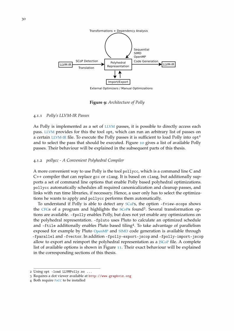
In the back end of Polly the original LLVM-IR is replaced by new code that is gen-erated following the possibly transformed polyhedral representation. At this step wecalculate an imperative program structure from the polyhedral representation and cre-ate the corresponding LLVM-IR instructions. Furthermore, we detect parallel loops thatcan either be executed with OpenMP to take advantage of thread level parallelism or re-placed with SIMD instructions, if fine grained parallelism is available. In future versionsof Polly, we plan to also integrate code generation for GPU based vector accelerators.Figure 9 illustrates the overall architecture of Polly.

4.1 how to use polly

There exist two ways to use Polly. One is to directly run one or several of Polly’s anal-ysis and optimization passes on existing LLVM-IR files. The other is to use pollycc, agcc/clang replacement that allows to conveniently compile C and C++ files with Polly.

1 http://pocc.sf.net

29

30

Figure 9: Architecture of Polly

4.1.1 Polly’s LLVM-IR Passes

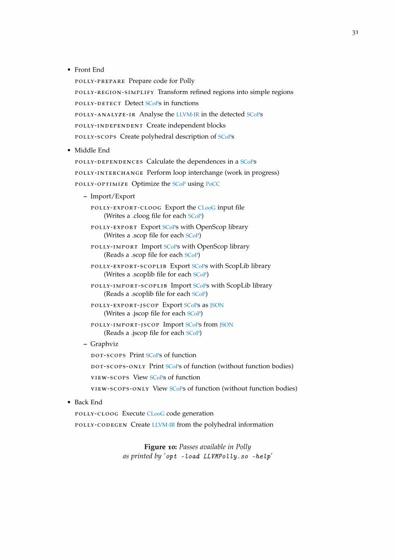
As Polly is implemented as a set of LLVM passes, it is possible to directly access eachpass. LLVM provides for this the tool opt, which can run an arbitrary list of passes ona certain LLVM-IR file. To execute the Polly passes it is sufficient to load Polly into opt2

and to select the pass that should be executed. Figure 10 gives a list of available Pollypasses. Their behaviour will be explained in the subsequent parts of this thesis.

4.1.2 pollycc - A Convenient Polyhedral Compiler

A more convenient way to use Polly is the tool pollycc, which is a command line C andC++ compiler that can replace gcc or clang. It is based on clang, but additionally sup-ports a set of command line options that enable Polly based polyhedral optimizations.pollycc automatically schedules all required canonicalization and cleanup passes, andlinks with run time libraries, if necessary. Hence, a user only has to select the optimiza-tions he wants to apply and pollycc performs them automatically.

To understand if Polly is able to detect any SCoPs, the option -fview-scops showsthe CFGs of a program and highlights the SCoPs found3. Several transformation op-tions are available. -fpolly enables Polly, but does not yet enable any optimizations onthe polyhedral representation. -fpluto uses Pluto to calculate an optimized scheduleand -ftile additionally enables Pluto based tiling4. To take advantage of parallelismexposed for example by Pluto OpenMP and SIMD code generation is available through-fparallel and -fvector. In addition -fpolly-export-jscop and -fpolly-import-jscopallow to export and reimport the polyhedral representation as a JSCoP file. A completelist of available options is shown in Figure 11. Their exact behaviour will be explainedin the corresponding sections of this thesis.

2 Using opt -load LLVMPolly.so ...3 Requires a dot viewer available at http://www.graphviz.org4 Both require PoCC to be installed

31

• Front End

polly-prepare Prepare code for Polly

polly-region-simplify Transform refined regions into simple regions

polly-detect Detect SCoPs in functions

polly-analyze-ir Analyse the LLVM-IR in the detected SCoPs

polly-independent Create independent blocks

polly-scops Create polyhedral description of SCoPs

• Middle End

polly-dependences Calculate the dependences in a SCoPs

polly-interchange Perform loop interchange (work in progress)

polly-optimize Optimize the SCoP using PoCC

– Import/Export

polly-export-cloog Export the CLooG input file(Writes a .cloog file for each SCoP)

polly-export Export SCoPs with OpenScop library(Writes a .scop file for each SCoP)

polly-import Import SCoPs with OpenScop library(Reads a .scop file for each SCoP)

polly-export-scoplib Export SCoPs with ScopLib library(Writes a .scoplib file for each SCoP)

polly-import-scoplib Import SCoPs with ScopLib library(Reads a .scoplib file for each SCoP)

polly-export-jscop Export SCoPs as JSON(Writes a .jscop file for each SCoP)

polly-import-jscop Import SCoPs from JSON(Reads a .jscop file for each SCoP)

– Graphviz

dot-scops Print SCoPs of function

dot-scops-only Print SCoPs of function (without function bodies)

view-scops View SCoPs of function

view-scops-only View SCoPs of function (without function bodies)

• Back End

polly-cloog Execute CLooG code generation

polly-codegen Create LLVM-IR from the polyhedral information

Figure 10: Passes available in Pollyas printed by ’opt -load LLVMPolly.so -help’

32

pollycc -husage: pollycc [-h] [-o OUTPUT] [-I INCLUDES] [-D PREPROCESSOR] [-l LIBRARIES]

[-L LIBRARYPATH] [-O {0,1,2,3,s}] [-S] [-emit-llvm][-std STANDARD] [-p] [-c] [-fpolly] [-fpluto] [-faligned][-fview-scops] [-fview-scops-only] [-ftile] [-fparallel][-fvector] [-fpolly-export] [-fpolly-import] [-commands] [-d][-v]files [files ...]

pollycc is a simple replacement for compiler drivers like gcc, clang or icc.It uses clang to compile C code and can optimize the code with Polly. It willeither produce an optimized binary or an optimized ’.o’ file.

positional arguments:files

optional arguments:-h, --help show this help message and exit-o OUTPUT the name of the output file-I INCLUDES include path to pass to clang-D PREPROCESSOR preprocessor directives to pass to clang-l LIBRARIES library flags to pass to the linker-L LIBRARYPATH library paths to pass to the linker-O {0,1,2,3,s} optimization level-S compile only; do not link or assemble-emit-llvm output LLVM-IR instead of assembly if -S is set-std STANDARD The C standard to use-p, --progress Show the compilation progress-c compile and assemble, but do not link-fpolly enable polly-fpluto enable pluto-faligned Assume aligned vector accesses-fview-scops Show the scops with graphviz-fview-scops-only Show the scops with graphviz (Only Basic Blocks)-ftile, -fpluto-tile enable pluto tiling-fparallel enable openmp code generation (in development)-fvector enable SIMD code generation (in development)-fpolly-export Export Polly jscop-fpolly-import Import Polly jscop-commands print command lines executed-d, --debug print debugging output-v, --version print version info

Figure 11: pollycc command line options

5L LV M - I R T O P O LY H E D R A L D E S C R I P T I O N

LLVM-IR has been designed for low level optimization. However, to hide unimportantinformation and to focus on a high-level optimization problem a more abstract represen-tation is often better suited. The scalar evolution analysis is for example a higher levelrepresentation used to abstract away the instructions needed to calculate a certain scalarvalue. It has proved to be very convenient for the optimization of scalar computations.For memory access and loop optimizations an abstraction based on a polyhedral modelpresented by Kelly and Pugh [29] is widely used. It hides imperative control flow struc-tures and allows to focus on the optimization of memory access patterns. Advancedoptimizers like CHiLL [15], LooPo [24] or Pluto [13] use such an abstraction to optimizefor data-locality and parallelism. An extended version of this polyhedral abstraction,called the Z-polyhedra model was presented by Gupta and Rajopadhye [26].

Polly uses a similar extended polyhedral representation, but it uses a different wayto obtain it. In contrast to most optimizers, which generate a polyhedral representationby analyzing a normal programming language, Polly analyzes a low level intermedi-ate representation. As a result, Polly is programming language independent and cantransparently support many constructs that would need special attention at the pro-gramming language level. Graphite [48] takes a similar approach by analyzing Gimple,the GCC intermediate representation. Even though Graphite and Polly share the gen-eral approach, there are notable differences between both. They arise directly from thedifferences of the intermediate representations, but also from the fact that Polly intro-duced new techniques to increase the amount of code that can be optimized and todecrease the amount of dependences that can block possible transformations. Further-more, Graphite does not yet support the Z-polyhedra extension.

In this chapter we describe the polyhedral representation used and we explain howit is derived from LLVM-IR. This includes a definition of the program parts that can bedescribed, an algorithm how to find such program parts and an explanation of howto create their polyhedral representation. Furthermore, we present a set of preparingtransformations that we use to increase to amount of code that we detect, to removeunneeded dependences and to simplify the implementation of Polly.1

1 The Polly front end was implemented in collaboration with Hongbin Zheng. His work was partiallyfounded by a Google Summer of Code 2010 scholarship where he was mentored by Tobias Grosser. Hiswork included code to verify if a region is a SCoP as well as code translating from LLVM-IR to the polyhedralrepresentation. He was also in charge of implementing the Polly automake and cmake build system aswell as parts of the test suite

33

34

for (int i = 0; i < 100 + n; i = i + 4) {A[i + 1] = B[i][3 * i] + A[i];

for (int j = i; j < 10 * i; j++)A[i + 1] = A[i] + A[i - n];

}

Figure 12: A valid SCoP (validity defined on ASTs)

5.1 what can be translated?

Traditionally polyhedral optimizations work on the Static Control Parts (SCoPs) of afunction. SCoPs are parts of a program in which all control flow and memory accesses areknown at compile time. As a result, they can be described in detail and a precise analysisis possible. Polly currently focuses on detecting and analysing SCoPs. Extensions tosupport non-statically known control flow were presented by Benabderrahmane et al.[12] and can be integrated in Polly, if needed.

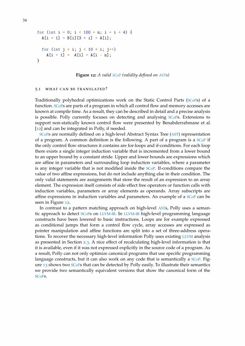
SCoPs are normally defined on a high-level Abstract Syntax Tree (AST) representationof a program. A common definition is the following. A part of a program is a SCoP ifthe only control flow structures it contains are for-loops and if-conditions. For each loopthere exists a single integer induction variable that is incremented from a lower boundto an upper bound by a constant stride. Upper and lower bounds are expressions whichare affine in parameters and surrounding loop induction variables, where a parameteris any integer variable that is not modified inside the SCoP. If-conditions compare thevalue of two affine expressions, but do not include anything else in their condition. Theonly valid statements are assignments that store the result of an expression to an arrayelement. The expression itself consists of side effect free operators or function calls withinduction variables, parameters or array elements as operands. Array subscripts areaffine expressions in induction variables and parameters. An example of a SCoP can beseen in Figure 12.

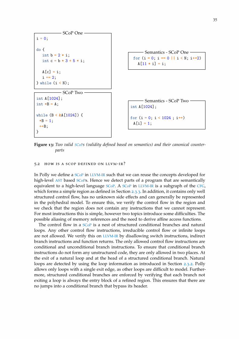
In contrast to a pattern matching approach on high-level ASTs, Polly uses a seman-tic approach to detect SCoPs on LLVM-IR. In LLVM-IR high-level programming languageconstructs have been lowered to basic instructions. Loops are for example expressedas conditional jumps that form a control flow cycle, array accesses are expressed aspointer manipulation and affine functions are split into a set of three-address opera-tions. To recover the necessary high-level information Polly uses existing LLVM analysisas presented in Section 2.3. A nice effect of recalculating high-level information is thatit is available, even if it was not expressed explicitly in the source code of a program. Asa result, Polly can not only optimize canonical programs that use specific programminglanguage constructs, but it can also work on any code that is semantically a SCoP. Fig-ure 13 shows two SCoPs that can be detected by Polly easily. To illustrate their semanticswe provide two semantically equivalent versions that show the canonical form of theSCoPs.

35

i = 0;

do {int b = 2 * i;int c = b * 3 + 5 * i;

A[c] = i;i += 2;

} while (i < N);

SCoP One

for (i = 0; i == 0 || i < N; i+=2)A[11 * i] = i;

Semantics - SCoP One

int A[1024];int *B = A;

while (B < &A[1024]) {*B = 1;++B;

}

SCoP Two

int A[1024];

for (i = 0; i < 1024 ; i++)A[i] = 1;

Semantics - SCoP Two

Figure 13: Two valid SCoPs (validity defined based on semantics) and their canonical counter-parts

5.2 how is a scop defined on llvm-ir?

In Polly we define a SCoP in LLVM-IR such that we can reuse the concepts developed forhigh-level AST based SCoPs. Hence we detect parts of a program that are semanticallyequivalent to a high-level language SCoP. A SCoP in LLVM-IR is a subgraph of the CFG,which forms a simple region as defined in Section 2.3.3. In addition, it contains only wellstructured control flow, has no unknown side effects and can generally be representedin the polyhedral model. To ensure this, we verify the control flow in the region andwe check that the region does not contain any instructions that we cannot represent.For most instructions this is simple, however two topics introduce some difficulties. Thepossible aliasing of memory references and the need to derive affine access functions.

The control flow in a SCoP is a nest of structured conditional branches and naturalloops. Any other control flow instructions, irreducible control flow or infinite loopsare not allowed. We verify this on LLVM-IR by disallowing switch instructions, indirectbranch instructions and function returns. The only allowed control flow instructions areconditional and unconditional branch instructions. To ensure that conditional branchinstructions do not form any unstructured code, they are only allowed in two places. Atthe exit of a natural loop and at the head of a structured conditional branch. Naturalloops are detected by using the loop information as introduced in Section 2.3.2. Pollyallows only loops with a single exit edge, as other loops are difficult to model. Further-more, structured conditional branches are enforced by verifying that each branch notexiting a loop is always the entry block of a refined region. This ensures that there areno jumps into a conditional branch that bypass its header.

36

To model the control flow in a SCoP statically it is necessary to know the number oftimes each loop is executed and to described this number with an affine expression.The natural loop analysis together with the scalar evolution analysis introduced in Sec-tion 2.3.4 can describe the number of loop iterations as a scalar evolution expression.In case a certain loop cannot be analyzed and consequently its loop iteration count isunknown, the loop can not be part of a SCoP. If the loop iteration count is available,we need to check, if the scalar evolution expression describing it can be translated intoan affine expression. This is the case if it only consists of integer constants, parame-ters, additions, multiplications with constants and add recurrences that have constantsteps. If parameters appear in the expression, we need to check that they are definedoutside of the SCoP and consequently do not change during the execution of the SCoP.We currently do not allow minimum, maximum, zero extend, sign extend or truncateexpressions even though they can conceptually be represented in the polyhedral model.A conditional branch is valid in a SCoP, if its condition is an integer comparison betweentwo affine expressions. Again, we use the scalar evolution analysis to get the scalar evo-lution expressions for each operand of the comparison and check whether each can berepresented as an affine expression.

To decide whether an instruction is valid in a SCoP, we verify that either no unknownside effects may happen or all side effects are known and can be represented in thepolyhedral model. Computational instructions, vector management instructions andtype conversion instructions in LLVM-IR are side effect free and can consequently ap-pear in a valid SCoP. Function calls are allowed if LLVM provides the information theyare side effect free and always return. The same holds for compiler internal intrinsics.Exception handling instructions on the other hand are always invalid, as they describecontrol flow that we cannot model statically. Load and store instructions are the onlyinstructions that can access memory. We currently require that a memory access can bedescribed by an expression that is affine in the number of loop iterations and parame-ters. We check this criterion by analyzing the scalar evolution of the pointer that definesthe memory location accessed. It must be affine following the conditions previously de-scribed. Additionally, the scalar evolution expression must contain a single parameter.This parameter is used as the base address of the memory access and defines the arraythat is accessed.

Base addresses in a SCoP must reference distinct memory spaces or they must beidentical. A memory space in this context is the set of memory elements that can beaccessed by adding an arbitrary offset to the base address. In case this is ensured, we canmodel the memory accesses as accesses to normal, non intersecting arrays. Fortunately,LLVM provides a set of alias analyses as described in Section 2.3.5, which give us exactlythis information. In case two base addresses are analyzed as must alias, they are identicaland, in case they are analyzed as no alias, the memory spaces that can be reached fromthem do not intersect. This may sound incorrect, as obviously a normal program hasjust one large address space and consequently a base address plus an integer offset isenough to reach any element in this space. However, programming languages like Cprovide sufficient information to ensure in many cases that an address derived fromone base address cannot yield an address derived from another base address.

The remaining restrictions are not conceptually necessary, but they simplify the over-all implementation of Polly. We require that every loop has a single, canonical induction

37

variable that starts at zero and is incremented with unit stride. Furthermore, any scalarvariable referenced must either be defined in the basic block it is used, it must be a loopinduction variable or it must be defined outside the SCoP. This ensures that no scalardependences exist between two different basic blocks. We later describe a preprocessingpass that can remove scalars that are used across basic blocks.

5.3 the polyhedral representation of a scop

Polly uses an abstract polyhedral description to represent a SCoP. It is based on integersets and maps as described in Section 3.1.

A polyhedral SCoP S = (context, [statements]) is a tuple consisting of a context anda list of statements. The context is an integer set that describes constraints on the pa-rameters of the SCoP like the fact that they are always positive or that there are certainrelations between parameters.

A statement Stmt = (name, domain, schedule, [accesses]) is described in Polly by aquadruple consisting of a name, a domain, a schedule and a list of accesses. It rep-resents a basic block BBStmt in the SCoP and is the smallest unit that can be scheduledindependently.

The domain of a statement is a named integer set that describes the set of differentloop iterations in which a statement is executed. Its name corresponds to the name ofthe statement. It has as many parameter dimensions as there are parameters in the SCoP.The number of set dimensions is equal to the number of loops that contain BBStmt andthat are contained in the SCoP. Each set dimension describes one loop induction variable,where the first dimension describes the outermost loop. An iteration vector is a singleelement of the domain. Together with a statement it defines a statement instance.

The schedule of a statement is an integer map that assigns to each iteration vectora multi-dimensional point in time. In the final code this time defines the executionorder of different statement instances. A statement instance (S1, v1) is executed beforea statement instance (S2, v2), if the iteration vector v1 is lexicographic smaller than theiteration vector v2. It is valid to assign to an iteration vector no execution time. Inthis case the corresponding statement instance is not executed at all. Assigning to oneiteration vector multiple execution times is at the moment not supported.

An access A = (kind, relation) is a pair that consists of the kind of the access andthe access relation. The kind is either read, write or may write. The access relation is aninteger map that maps from the domain of a statement into a named, possibly multi-dimensional memory space. The name of the memory space is used to distinguish be-tween accesses to distinct memory spaces. The access relation can be an affine function,but also any other relation that can be expressed with integer maps. Hence, an accessmay touch either a single element or a set of memory elements. If two accesses point tomemory spaces with different names.

Figure 14 shows an example of a high-level program represented as a SCoP. It showsthe domains, schedules and the accesses for each of the statements. For StmtA1 the do-main is one-dimensional as the statement is surrounded by only one loop. For this loopthe constraints i ≥ 0 and i ≤ N are added to the iteration space. In addition the con-straint i ≤ N − 50 is added as StmtA1 is also part of a conditional branch. The someholds for StmtA2 , but as StmtA2 is part of the else-branch of the condition the reverted

38

void scop(long N) {long i, j;

for (i = 0; i < N; i++) {if (i <= N - 50)

A[5*i] = 1; // Stmt_A1else

A[3*i] = 2; // Stmt_A2

for (j = 0; j < N; j++) {B[i][2*j] = 3; // Stmt_B

}}

}

Context = [N]→ {}

DStmtA1= [N]→ {StmtA1 [i] : i ≥ 0∧ i ≤ N ∧ i ≤ N − 50}

SStmtA1= {StmtA1 [i]→ Θ[0, i, 0, 0, 0]}

AStmtA1= {StmtA1 [i]→ A[5i]}

DStmtA2= [N]→ {StmtA2 [i] : i ≥ 0∧ i ≤ N ∧ i > N − 50}

SStmtA2= {StmtA2 [i]→ Θ[0, i, 1, 0, 0]}

AStmtA2= {StmtA2 [i]→ A[3i]}

DStmtB = [N]→ {StmtB[i] : i ≥ 0∧ i ≤ N ∧ j ≥ 0∧ j ≤ N}SStmtB = {StmtB[i, j]→ Θ[0, i, 2, j, 0]}AStmtB = {StmtB[i, j]→ B[i][2j]}

Figure 14: An example of a SCoP and its polyhedral representation.

39

constraint i > N − 50 is added to its domain. StmtB is surrounded by two loops, so atwo-dimensional domain is created that contains constraints for both loops. The sched-ules of the statements map each statement iteration into a five-dimensional timescale,which ensures the same execution order as in the original code. Furthermore, withAStmtA1

, AStmtA2and AStmtB three memory accesses are defined. The first two represent

accesses to a one-dimensional array A, the last one an access to a two-dimensional arrayB.

5.4 how to create the polyhedral representation from llvm-ir

A region of LLVM-IR code that forms a valid SCoP is translated into a polyhedral rep-resentation by treating it conceptually as a high-level SCoP. We initialize the context ofthe SCoP with an unconstrained integer set. This integer set has zero set dimensionsand as many parameter dimensions as there are parameters in the SCoP. To determinethe number of parameters the scalar evolution of all addresses used in load or store in-structions is calculated as well as a scalar evolution expression describing the iterationcount for every loop and one for each value used in a condition of a branch instruction.The scalar evolution expressions are then scanned for the largest subexpressions, thatare not modified inside the region. These form the parameters of the SCoP. Polly doesnot yet calculate relations between parameters, such that the context remains currentlyunconstrained.

The statements of a SCoP are formed by the different basic blocks in the CFG. As,besides memory accesses, basic blocks are side effect free, we only create polyhedralstatements for the basic blocks that contain at least one load or store instruction. For abasic block BBStmt the name of a statement is a unique string set to the name of BBStmt.

The domain of a statement for BBStmt is created as follows. We add for each loopsurrounding BBStmt one constraint ivi ≥ 0 as its lower bound and another constraintivi ≤ ”number o f loop iterations”− 1 as its upper bound. Furthermore, if BBStmt is in aconditional branch, we add the corresponding condition to the domain of the statement.This is the case, if there exists a basic block BBCond that has a conditional statement,dominates BBStmt and the immediate postdominator of BBCond post dominates BBStmt,but is not BBStmt. The same property is used to understand, if a basic block that is partof a loop is before or after the basic block exiting the loop. In case it is after the exitingblock, the exiting condition is also added to the domain to model the fact that BBStmt isnot executed during the last loop iteration.

The initial schedule for each statement has as many input dimensions Ii as the domainhas set dimension and it has 2d + 1 output dimensions Oo, where d is the maximal loopdepth in the SCoP. It contains a set of constraints Ii = O2i+1 that set the values of the oddoutput dimensions to the values of the input dimensions. These constraints enforce fordifferent instances of a single statement the same execution order as in the original loopnest. To ensure the correct execution order between instances of different statementsthe even dimensions are used to define the textual order of the statements. The value atdimension 2l is determined by topologically sorting the elements surrounded by exactlyl loops. These can either be basic blocks or control flow regions that represent loops atlevel l + 1. For all basic blocks contained in loop regions at level l + 1 the value of

40

dimension 2l is set to the value assigned to the loop region. In case no loop exists todefine a dimension, the dimension is set to zero.

To calculate the accesses of a statement Polly analyzes all load and store instructions.Load instructions are represented as read accesses and store instructions as write ac-cesses. For each load and store instruction we extract the scalar that defines the memoryaddress and retrieve its scalar evolution. The scalar evolution expression is then trans-lated into an affine expression. Here we use the parameter in the scalar evolution expres-sion as the base address of the memory access. This base address is also used to namethe memory space which ensures that accesses to different parts of the memory aremodeled as accesses to different arrays. Polly currently only creates single-dimensionalaccess functions. This is sufficient to represent single-dimensional arrays, but also multi-dimensional accesses, with statically know size. Support for multi-dimensional variable-size arrays is planned.

Figure 15 shows the steps from C code over LLVM-IR to our polyhedral representation.It starts with C code that is then lowered to a set of basic blocks. These blocks containLLVM-IR instructions that calculate loop bounds, induction variables and array accessfunctions. For instance the address of the memory accessed in StmtB is calculated andthe result of this calculation in stored in the virtual register %scevgep. To derive theaccess function from %scevgep we calculate the scalar evolution expression {@B, +, (2 ∗sizeo f ( f loat))}<%bb1>, which describes the memory address accessed. This expressionis then split into a base element B and a single dimensional access function 2× i, wherei is a virtual induction variable counting the number of loop iterations. As %indvar is acanonical induction variable, its value is equivalent to i. To calculate the domain of thestatement we call the scalar evolution analysis and ask for the number of times the loopback edge is executed. In this example the resulting expressing is the integer constant99. To derive the number of loop iterations we simply add one. With the knowledge,that canonical induction variables always start at zero, we get the domain {StmtB[i] :0 ≤ i < 100}.

5.5 how to detect maximal scops

Polly uses a structured approach to detect a set of maximal SCoPs. In general a functionmay contain various SCoPs which overlap or are nested. Optimizing overlapping ornested SCoPs is difficult. A SCoP that was already optimized by Polly, can sometimesnot be recognized again or, in case it can, code that was already optimized will beoptimized again. To avoid such redundant calculations and to maximize the space ofpossible transformations inside a SCoP, we detect SCoPs that are maximal and that cannotbe enlarged further.

Polly uses the region tree described in Section 2.3.3 to detect maximal SCoPs. Thefirst step is to find a set of maximal canonical regions that are SCoPs. This is done bywalking down the region tree. Starting from the largest possible canonical region wedescend into the tree. If a region forms a SCoP, we add it to the set of valid SCoPs anddo not further descend in this part of the region tree. In case a region is no valid SCoP,we continue the search by examining its children. After the walk on the region tree,we have a set of maximal, canonical regions that form valid SCoPs. Yet, a SCoP mayalso be described by a non-canonical region. To get the set of maximal, not necessarily

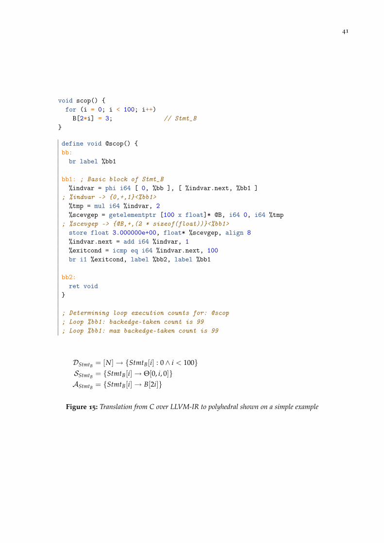
41

void scop() {for (i = 0; i < 100; i++)

B[2*i] = 3; // Stmt_B}

define void @scop() {bb:

br label %bb1

bb1: ; Basic block of Stmt_B%indvar = phi i64 [ 0, %bb ], [ %indvar.next, %bb1 ]

; %indvar -> {0,+,1}<%bb1>%tmp = mul i64 %indvar, 2%scevgep = getelementptr [100 x float]* @B, i64 0, i64 %tmp

; %scevgep -> {@B,+,(2 * sizeof(float))}<%bb1>store float 3.000000e+00, float* %scevgep, align 8%indvar.next = add i64 %indvar, 1%exitcond = icmp eq i64 %indvar.next, 100br i1 %exitcond, label %bb2, label %bb1

bb2:ret void

}

; Determining loop execution counts for: @scop; Loop %bb1: backedge-taken count is 99; Loop %bb1: max backedge-taken count is 99

DStmtB = [N]→ {StmtB[i] : 0∧ i < 100}SStmtB = {StmtB[i]→ Θ[0, i, 0]}AStmtB = {StmtB[i]→ B[2i]}

Figure 15: Translation from C over LLVM-IR to polyhedral shown on a simple example

42

1

A

B

C1

C2

1

2

3

4

5

6

7

2

A

B

C1

C2

1

2

3

4

5

6

7

3

A

B

C1’

C2

1

2

3

4

5

6

7

4

A

B

C1’’

1

2

3

4

5

6

7

Figure 16: Region based SCoP detection

canonical regions that form SCoPs we enlarge the canonical regions by merging themwith subsequent regions. This is done as long as the resulting regions still form validSCoPs. When no region can be further extended, we have a set of maximal SCoPs.

Figure 16 shows in steps how we detect the set of maximal SCoPs in a function. Westart at the outermost region A. It does not form a valid SCoP, as it contains basic blocktwo, which is marked as difficult. We than check its child region, region B. It is alsoinvalid, as it still contains basic block two. However, when we try the children of B,C1 and C2, we successfully find two regions that are valid SCoPs. These are the largestcanonical regions that form valid SCoPs. To further increase their size we start to mergeregions. We begin with C1 and merge basic block four to create C1′. This is valid asbasic block four forms a (very simple) region. Next, we merge region C2. The resultingC1′′ now contains basic block three, four and five. It cannot be enlarged further, as thereexists no region that starts at basic block 6. Even basic block 6 forms no region, as it hastwo exit edges, that terminate at different basic blocks. Hence, for our example the setof maximal SCoPs is {C1′′}.

43

5.6 preparing transformations

A set of preparing transformations is necessary to increase the coverage of Polly. Polly’sfront end is on purpose kept simple and often handles LLVM-IR that is in a canonicalform. To ensure that LLVM-IR which does not match this form can be optimized, theLLVM-IR of a program is canonicalized before it is passed to the SCoP detection. Canoni-calization is done by a set of transformations already available in LLVM and some trans-formations especially developed for Polly.

5.6.1 LLVM canonicalization passes

The set of LLVM transformation and canonicalization passes used in Polly is derivedfrom the first half of the passes used in clang -O3. It contains a basic alias analysis,memory to register promotion, simplification of library calls, instruction simplification,tail call elimination, loop simplification, loop closed ssa form calculation, loop rotation,loop unswitch, and induction variable canonicalization. The most important passes havebeen described in Section 2.4. Furthermore, a pass to transform refined regions intosimple regions is used. This pass is conceptually not necessary, but it simplifies theimplementation of Polly.

5.6.2 Create Independent Basic Blocks

The independent block pass in Polly removes unnecessary inter basic block depen-dences introduced by scalar values and creates basic blocks that can be freely scheduled.Furthermore, the independent block pass promotes scalar dependences that cannot beremoved into loads and stores to single element arrays. This ensures that the only scalardependences that remain are references to induction variables or parameters. As induc-tion variables and parameters are replaced during code generation, Polly does not needto perform any special handling for scalar dependences. All basic blocks can be movedfreely during code generation.

Unnecessary dependences are regularly introduced due to calculations of array in-dexes, branch conditions or loop bounds which are often spread over several basicblocks. To remove such dependences, we duplicate all trivial scalar operations in eachbasic block. This means, if an operation does not read or write memory and does nothave any side effects, its results are not transfered from another basic block, but it is en-tirely recalculated in each basic block. The only exceptions are PHI-Nodes, parametersand induction variables, which are not touched at all.

The recalculation of scalar values introduces a notable amount of redundant code andwould normally slow down the code a lot. However, as will be later shown in Section 9,scheduling the normal LLVM cleanup passes after Polly is sufficient to remove theseredundant calculations.

Figure 17 shows a SCoP that has several scalar dependences from bb1 to bb2, bb3, bb4

and bb5 which block possible transformations. They are introduced through the scalarvariables %scevgepA, %scevgepB, %i.0 and %valAdd. By applying the independentblock pass we move trivial calculations directly into bb2, bb3 and bb4. As can be seenin Figure 18, this introduces redundant calculations for %scevgepA.1 and %scevgepA.2.

44

However, the updated basic blocks now only depend on the value of the induction vari-able. The scalar dependency introduced by %valAdd cannot be removed by moving itscalculation to bb5, as the load from %scevgepB cannot be moved. Consequently thisscalar dependency cannot be eliminated, but it is promoted to a memory dependency.Overall the independent block pass removes all scalar dependences and it ensures thatonly the dependences that cannot be eliminated will show up in the final memory de-pendency graph.

45

CFG for 'foo' function

bb: br label %bb1

bb1: %indvar = phi i64 [ %indvar.next, %bb6 ], [ 0, %bb ] %scevgepA = getelementptr [1024 x i32]* @A, i64 0, i64 %indvar %scevgepB = getelementptr [1024 x i32]* @B, i64 0, i64 %indvar %i.0 = trunc i64 %indvar to i32 %exitcond = icmp ne i64 %indvar, 1024 %val = load i32* %scevgepB %valAdd = add i32 %val, 15 br i1 %exitcond, label %bb2, label %bb7

T F

bb2: %tmp = icmp sle i32 %i.0, 512 br i1 %tmp, label %bb3, label %bb4

T F

bb7: ret void

bb3: store i32 1, i32* %scevgepA br label %bb5

bb4: store i32 2, i32* %scevgepA br label %bb5

bb5: store i32 %valAdd, i32* %scevgepB br label %bb6

bb6: %indvar.next = add i64 %indvar, 1 br label %bb1

Figure 17: Simple SCoP before independent block pass

46

CFG

for '

foo'

func

tion

bb:

%va

l.s2a

= a

lloca

i32

br l

abel

%bb

1

bb1:

%

indv

ar =

phi

i64

[ %in

dvar

.nex

t, %

bb6

], [ 0

, %bb

] %

scev

gepB

= g

etel

emen

tptr

[102

4 x

i32]

* @

B, i

64 0

, i64

%in

dvar

%ex

itcon

d =

icm

p ne

i64

%in

dvar

, 102

4 %

val =

load

i32*

%sc

evge

pB s

tore

i32

%va

l, i3

2* %

val.s

2a b

r i1

%ex

itcon

d, la

bel %

bb2,

labe

l %bb

7

TF

bb2:

%

i.0 =

trun

c i6

4 %

indv

ar to

i32

%tm

p =

icm

p sl

e i3

2 %

i.0, 5

12 b

r i1

%tm

p, la

bel %

bb3,

labe

l %bb

4

TF

bb7:

re

t voi

d

bb3:

%

scev

gepA

.1 =

get

elem

entp

tr [1

024

x i3

2]*

@A

, i64

0, i

64 %

indv

ar s

tore

i32

1, i3

2* %

scev

gepA

.1 b

r lab

el %

bb5

bb4:

%

scev

gepA

.2 =

get

elem

entp

tr [1

024

x i3

2]*

@A

, i64

0, i

64 %

indv

ar s

tore

i32

2, i3

2* %

scev

gepA

.2 b

r lab

el %

bb5

bb5:

%

val.l

oada

rray

= lo

ad i3

2* %

val.s

2a %

valA

dd =

add

i32

%va

l.loa

darr

ay, 1

5 %

scev

gepB

.2 =

get

elem

entp

tr [1

024

x i3

2]*

@B

, i64

0, i

64 %

indv

ar s

tore

i32

%va

lAdd

, i32

* %

scev

gepB

.2 b

r lab

el %

bb6

bb6:

%

indv

ar.n

ext =

add

i64

%in

dvar

, 1 b

r lab

el %

bb1

Figure 18: Simple SCoP after independent block pass

6P O LY H E D R A L O P T I M I Z AT I O N S

After showing how SCoPs are represented in Polly, we describe how they can be opti-mized. Basically there are two ways to optimize a SCoP. One is changing the executionorder of the statement instances in the SCoP, the other is changing the memory locationsthey access. Polly currently focuses on changes of the execution order. Classical looptransformations like interchange, tiling, fusion and fission but also advanced transfor-mations [13] change the execution order. Support for optimizations that change dataaccesses as proposed by Kandemir et al. [28] and Clauss and Meister [16] is planned.

In Polly changes to the execution order are expressed by modifying the schedulesof the statements. Access relations and iteration domains are read-only. This seems tobe obvious, as only the schedule is defining the execution times. However, previousapproaches as for example presented by Girbal et al. [23] had difficulties to expresstransformations like tiling or index set splitting without changes to the domain. Thosedifficulties do not arise in Polly, as the integer maps used to define the schedules areexpressive enough to describe those transformations.

There are two ways the schedules can be changed. Either they can be replaced byschedules that are recalculated from scratch or the schedules can be modified by a setof transformations. In Polly a transformation is an integer map that maps from theoriginal execution time to a new execution time. It is performed by applying it to theschedules of the statements that should be transformed. Two transformations can becomposed by applying the second on the range of the first.

In this Chapter we describe how classical loop transformations can be expressed, howoptimizations can be applied manually, how external optimizers can be connected andhow dependency analysis is performed.

6.1 transformations on the polyhedral representation

In this section we present how classical loop transformations like interchange, fission,strip mining, unroll and jam or loop blocking can be expressed as scheduling trans-formations. Furthermore, we show how partial transformations that happen commonlyafter index set splitting [25] can be expressed.

47

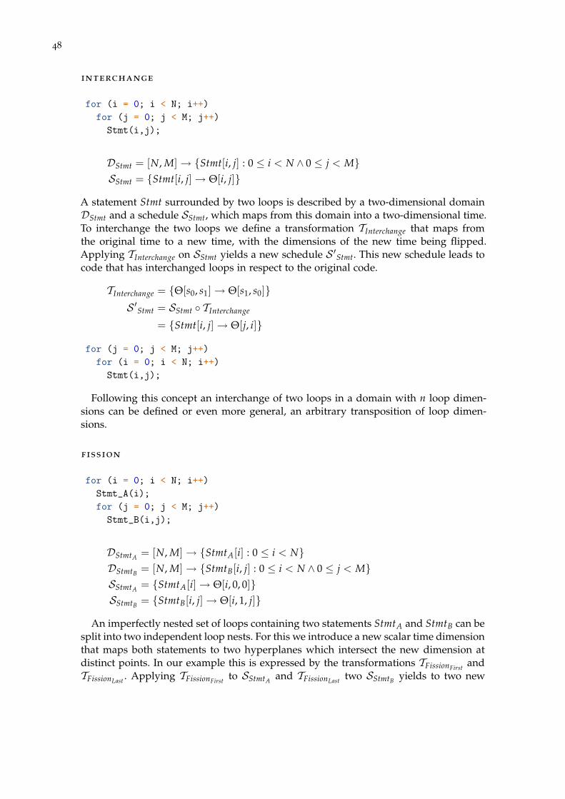
48

interchange

for (i = 0; i < N; i++)for (j = 0; j < M; j++)

Stmt(i,j);

DStmt = [N, M]→ {Stmt[i, j] : 0 ≤ i < N ∧ 0 ≤ j < M}SStmt = {Stmt[i, j]→ Θ[i, j]}

A statement Stmt surrounded by two loops is described by a two-dimensional domainDStmt and a schedule SStmt, which maps from this domain into a two-dimensional time.To interchange the two loops we define a transformation TInterchange that maps fromthe original time to a new time, with the dimensions of the new time being flipped.Applying TInterchange on SStmt yields a new schedule S ′Stmt. This new schedule leads tocode that has interchanged loops in respect to the original code.

TInterchange = {Θ[s0, s1]→ Θ[s1, s0]}S ′Stmt = SStmt ◦ TInterchange

= {Stmt[i, j]→ Θ[j, i]}

for (j = 0; j < M; j++)for (i = 0; i < N; i++)

Stmt(i,j);

Following this concept an interchange of two loops in a domain with n loop dimen-sions can be defined or even more general, an arbitrary transposition of loop dimen-sions.

fission

for (i = 0; i < N; i++)Stmt_A(i);for (j = 0; j < M; j++)

Stmt_B(i,j);

DStmtA = [N, M]→ {StmtA[i] : 0 ≤ i < N}DStmtB = [N, M]→ {StmtB[i, j] : 0 ≤ i < N ∧ 0 ≤ j < M}SStmtA = {StmtA[i]→ Θ[i, 0, 0]}SStmtB = {StmtB[i, j]→ Θ[i, 1, j]}

An imperfectly nested set of loops containing two statements StmtA and StmtB can besplit into two independent loop nests. For this we introduce a new scalar time dimensionthat maps both statements to two hyperplanes which intersect the new dimension atdistinct points. In our example this is expressed by the transformations TFissionFirst andTFissionLast . Applying TFissionFirst to SStmtA and TFissionLast two SStmtB yields to two new

49

schedules S ′StmtA and S ′StmtB . They lead to code to execute the two statements in twodistinct loop nests.

TFissionFirst = {Θ[s0, s1, s2]→ Θ[0, s0, s1, s2]}TFissionLast = {Θ[s0, s1, s2]→ Θ[1, s0, s1, s2]}S ′StmtA = SStmtA ◦ TFissionFirst

= {StmtA[i]→ Θ[0, i, 0, 0]}S ′StmtB = SStmtB ◦ TFissionLast

= {StmtB[i, j]→ Θ[1, i, 1, j]}

for (i = 0; i < N; i++)Stmt_A(i);

for (i = 0; i < N; i++)for (j = 0; j < M; j++)

Stmt_B(i,j);

Similarly it is possible to split loop nests starting at a loop depth of n. In this case thenew scalar dimension is not inserted at the first time dimension (counting from one),but at the time dimension preceding the loop dimension that should be split.

strip mining

for (i = 0; i < N; i++)Stmt(j);

DStmt = [N]→ {Stmt[i] : 0 ≤ i < N}SStmt = {Stmt[i]→ Θ[i]}

To execute a single loop section wise it can be transformed into a nest of two loopsby applying strip mining. This transformation is not profitable on its own, but it is thebase for transformations like partial unrolling, loop blocking or unroll and jam. In ourexample we want to execute sections of four loop iterations. Each section should benumbered by an integer t where t mod 4 = 0 holds and it should enumerate the itera-tions from t to t + 3. This is specified by transformation TStripMine. Applying TStripMineto SStmt yields to the new schedule S ′Stmt and generates the expected loop nest.

TStripMine = {Θ[s0]→ Θ[t, s0] : t mod 4 = 0∧ t ≤ s0 < t + 4}S ′Stmt = S ′Stmt ◦ TStripMine

= {Stmt[s0]→ Θ[t, s0] : t mod 4 = 0∧ t ≤ s0 < t + 4}

for (ii = 0; ii < N; ii+=4)for (i = ii; i < min(N, ii+4); i++)

Stmt(i)

50

unroll-and-jam

for (i = 0; i < N; i++)for (j = 0; j < M; j++)

Stmt(i,j)

Context = [N, M]→ {[] : N mod 4 = 0}DStmt = [N, M]→ {Stmt[i, j] : 0 ≤ i < N ∧ 0 ≤ j < M}SStmt = {Stmt[i, j]→ Θ[i, j]}

Unroll-and-jam is a transformation that (partially) unrolls a non-innermost loop andthen subsequently fuses the created loop nests back together. We express this as a poly-hedral transformation that creates an innermost loop with a constant number of iter-ations. This loop can then be unrolled by a simple code generation pass or it can betransformed to SIMD code, if parallel execution is valid. In case the unroll factor doesnot divide the number of original loop iterations in whole numbers, some preparingtransformations are necessary to apply unroll and jam.

To perform the loop transformation part of unroll and jam we create the transforma-tions TStripMine and TInterchange which are conceptually already known. Combining bothyields to the transformation TUnrollAndJam, which applied to SStmt produces the scheduleS ′Stmt and generates the expected loop nest.

TStripMine = {Θ[s0, s1]→ Θ[t, s0, s1] : t mod 4 = 0∧ t ≤ s0 < t + 4}TInterchange = {Θ[s0, s1, s2]→ Θ[s0, s2, s1]}

TUnrollAndJam = TStripMine ◦ TInterchange

= {Θ[s0, s1]→ Θ[t, s1, s0] : t mod 4 = 0∧ t ≤ s0 < t + 4}S ′Stmt = SStmt ◦ TUnrollAndJam

= {Stmt[i, j]→ Θ[t, j, i] : t mod 4 = 0∧ t ≤ i < t + 4}

for (ii = 0; ii < N; ii+=4)for (j = 0; j < M; j++)

for (i = ii; i < ii+4; i++)Stmt(i,j);

loop blocking

for (i = 0; i < N; i++)for (j = 0; j < M; j++)

Stmt(i,j);

DStmt = [N, M]→ {Stmt[i, j] : 0 ≤ i < N ∧ 0 ≤ j < M}SStmt = {Stmt[i, j]→ Θ[i, j]}

Loop blocking is a transformation that can increase data locality by executing a loopnest block wise. It can be represented by combining the transformations TStripMineOuter ,TStripMineInner and TInterchange to a single transformation TBlock.

51

TStripMineOuter = {Θ[s0, s1]→ Θ[t, s0, s1] : t mod 4 = 0∧ t ≤ s0 ≤ t + 3}TStripMineInner = {Θ[s0, s1, s2]→ Θ[s0, s1, t, s2] : t mod 4 = 0∧ t ≤ s2 ≤ t + 3}TInterchange = {Θ[s0, s1, s2, s3]→ Θ[s0, s2, s1, s3]}

TBlock = TStripMineOuter ◦ TStripMineInner ◦ TInterchange

= {Θ[s0, s1]→ Θ[t0, t1, s0, s1] : t0 mod 4 = 0∧ t0 ≤ s0 < t0 + 4

∧ t1 mod 4 = 0∧ t1 ≤ s1 < t1 + 4}S ′Stmt = SStmt ◦ TBlock

= {Stmt[i, j]→ Θ[ti, tj, i, j] : ti mod 4 = 0∧ ti ≤ i < ti + 4

∧ tj mod 4 = 0∧ tj ≤ j < tj + 4}

for (ii = 0; ii < M; ii+=4)for (jj = 0; jj < N; jj+=4)

for (i = ii; i < min(M, ii+4); i++)for (j = jj; j < min(N, jj+4); j++)

Stmt(i,j);

partial transformations - index set splitting

for (i = 0; i <= 2 * N; i++)A[i] = A[2 * N - 1]; // Stmt

DStmt = [N]→ {Stmt[i, j] : 0 ≤ i ≤ N}SStmt = {Stmt[i]→ Θ[i]}

In some cases it is beneficial to split the iteration domain of a statement and to createfor different parts of the iteration domain different schedules. Such a transformation isknown as index set splitting as presented by Griebl et al. [25]. To represent it in Polly,there is no need to create two separate statements. Instead we define a transformationthat applies only to a part of the index space. We call such a transformation partialtransformation.

In our example we have a single loop that cannot be executed in parallel becauseof dependencies between the lower and the upper half of the iteration space. However,if we apply loop fission and split the lower and the upper part of the iteration spaceinto two separate loops, two fully parallel loops can be generated. To describe this wedefine two transformations, that generate a new time dimension on which we split theiterations. TFissionFirst maps the lower part of the iteration space to an earlier time in thisdimension, and TFissionLast maps the upper part of the iteration space to a later time inthis dimension. Both can be merged to a single transformation TFissionCombined , which issubsequently applied to SStmt. This results in the new schedule S ′Stmt which producesthe expected parallel loops.

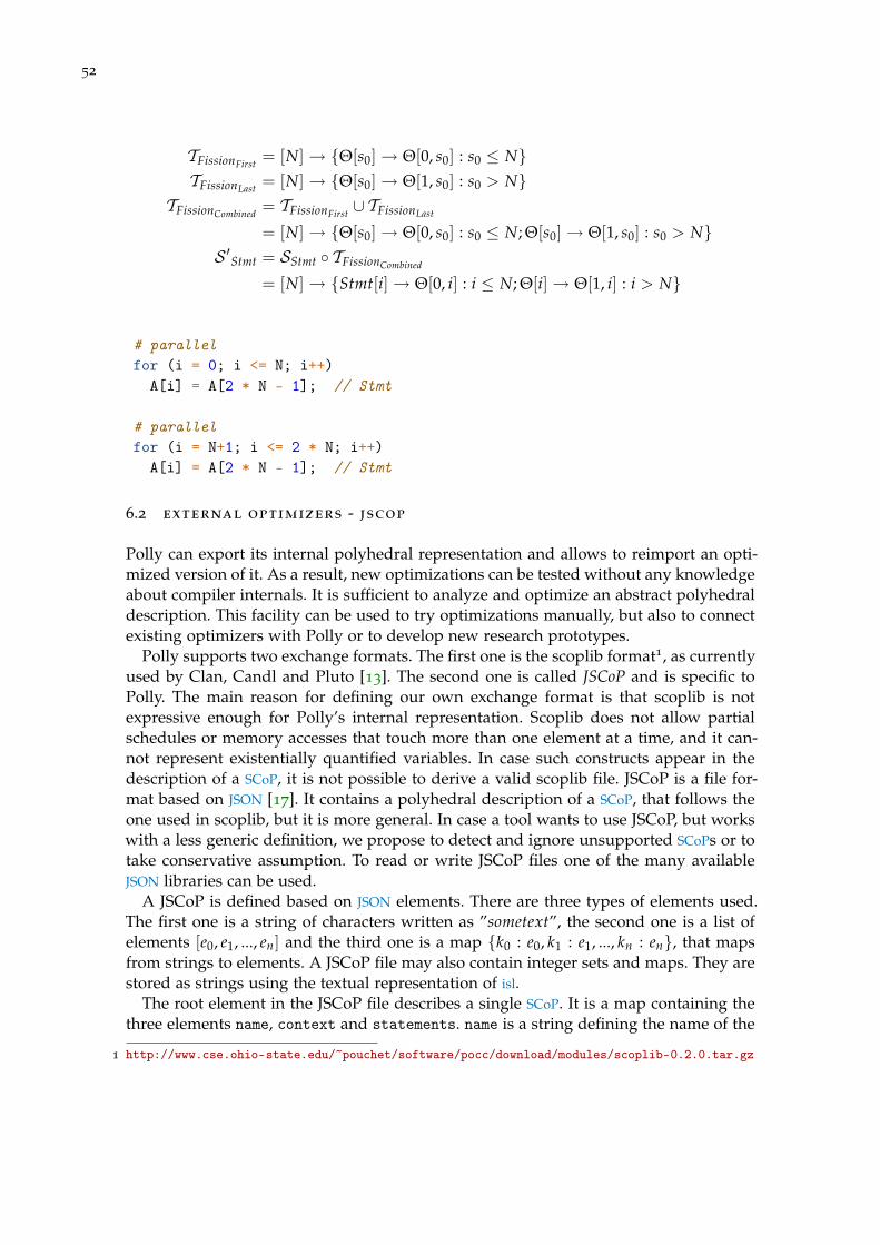
52

TFissionFirst = [N]→ {Θ[s0]→ Θ[0, s0] : s0 ≤ N}TFissionLast = [N]→ {Θ[s0]→ Θ[1, s0] : s0 > N}

TFissionCombined = TFissionFirst ∪ TFissionLast

= [N]→ {Θ[s0]→ Θ[0, s0] : s0 ≤ N; Θ[s0]→ Θ[1, s0] : s0 > N}S ′Stmt = SStmt ◦ TFissionCombined

= [N]→ {Stmt[i]→ Θ[0, i] : i ≤ N; Θ[i]→ Θ[1, i] : i > N}

# parallelfor (i = 0; i <= N; i++)

A[i] = A[2 * N - 1]; // Stmt

# parallelfor (i = N+1; i <= 2 * N; i++)

A[i] = A[2 * N - 1]; // Stmt

6.2 external optimizers - jscop

Polly can export its internal polyhedral representation and allows to reimport an opti-mized version of it. As a result, new optimizations can be tested without any knowledgeabout compiler internals. It is sufficient to analyze and optimize an abstract polyhedraldescription. This facility can be used to try optimizations manually, but also to connectexisting optimizers with Polly or to develop new research prototypes.

Polly supports two exchange formats. The first one is the scoplib format1, as currentlyused by Clan, Candl and Pluto [13]. The second one is called JSCoP and is specific toPolly. The main reason for defining our own exchange format is that scoplib is notexpressive enough for Polly’s internal representation. Scoplib does not allow partialschedules or memory accesses that touch more than one element at a time, and it can-not represent existentially quantified variables. In case such constructs appear in thedescription of a SCoP, it is not possible to derive a valid scoplib file. JSCoP is a file for-mat based on JSON [17]. It contains a polyhedral description of a SCoP, that follows theone used in scoplib, but it is more general. In case a tool wants to use JSCoP, but workswith a less generic definition, we propose to detect and ignore unsupported SCoPs or totake conservative assumption. To read or write JSCoP files one of the many availableJSON libraries can be used.

A JSCoP is defined based on JSON elements. There are three types of elements used.The first one is a string of characters written as ”sometext”, the second one is a list ofelements [e0, e1, ..., en] and the third one is a map {k0 : e0, k1 : e1, ..., kn : en}, that mapsfrom strings to elements. A JSCoP file may also contain integer sets and maps. They arestored as strings using the textual representation of isl.

The root element in the JSCoP file describes a single SCoP. It is a map containing thethree elements name, context and statements. name is a string defining the name of the

1 http://www.cse.ohio-state.edu/~pouchet/software/pocc/download/modules/scoplib-0.2.0.tar.gz

53

{"name": "body => loop.end","context": "[N] -> { []: N >= 0 }","statements": [{

"name": "Stmt_body","domain": "[N] -> { Stmt_body[i0, i1, i2] : 0 <= i0, i1, i2 <= N }","schedule": "[N] -> { Stmt_body[i0, i1, i2] -> scattering[i0, i1, i2] }","accesses": [{

"kind": "read","relation": "[N] -> { Stmt_body[i0, i1, i2] -> MemRef_C[i0][i1] }"

},{

"kind": "read","relation": "[N] -> { Stmt_body[i0, i1, i2] -> MemRef_A[i0][i2] }"

},{

"kind": "read","relation": "[N] -> { Stmt_body[i0, i1, i2] -> MemRef_B[i1][i2] }"

},{

"kind": "write","relation": "[N] -> { Stmt_body[i0, i1, i2] -> MemRef_C[i0][i1] }"

}]}]

}

Figure 19: JSCoP file of a matrix multiplication kernel

54

SCoP, context is an integer set describing the set of valid parameters and statements isa list of the statements as subsequently defined. context has zero set dimensions andas many parameter dimensions as there are parameters in the SCoP.

A statement is a map containing four elements called name, domain, schedule andaccesses. name is a unique string that identifies a statement and domain is the iterationspace of the statement. The iteration space describes the set of statement instances thatwill be executed. It is represented as an integer set, which has as many parameterdimensions as the context of the SCoP and as many set set dimensions as there areloops that surround the statement. The space defined by domain is named with thename of the statement. schedule is a map that defines for each statement instance amulti-dimensional execution time. It has as many input dimensions as domain has setdimension and an arbitrary number of output dimensions Yet, all schedules in the SCoPmust have the same number of output dimensions. The name of the output space is’scattering’. accesses is a list of the memory accesses of the statement.

A memory access is a map containing two elements called type and relation. Thetype can be read, write or maywrite. It is read if the statement must or may read thismemory. It is write if the statement must write to this memory and it is maywrite if thestatement may or may not write to this memory. If a statement reads and writes identicalmemory, two accesses are generated, one for the read and one for the write access.relation defines the memory accessed. It is a mapping from the statement instanceexecuted to the memory element accessed. The input space of the access relation hasthe same number of dimensions as the domain of the statement and is also identicallynamed. The output space defines the array elements accessed. It has a unique namefor each distinct array accessed in the SCoP and describes a possibly multi-dimensionalspace of array elements.

All data structures are read-only, except the schedules of the statements. All transfor-mations are expressed by modifying the schedules of the statements. To support arrayexpansion or memory access transformations we plan to also allow updates of the ac-cess relations. Figure 19 shows an example of a JSCoP file of a matrix multiplicationkernel.

6.3 dependency analysis

Polly provides an advanced dependency analysis implemented on top of the isl pro-vided data flow analysis. The isl data flow analysis is based on techniques developed byFeautrier [20] with influences from Pugh and Wonnacott [39]. It includes full supportfor existentially quantified variables, can be restricted to non-transitive dependencesand allows full access relations as well as may-write accesses. We believe the last twofeatures do no exist in most implementations of data-dependency analyses.

Polly currently uses the dependency analysis to calculate read-after-write, write-after-write and write-after-read dependences. The dependences are calculated from the poly-hedral description. We pass the access relations and types, the domains and the sched-ules of all statements in the SCoP to the isl data flow analysis. isl then calculates exact,non-transitive data flow dependences as well as the statement instances that do not haveany source and consequently depend on the state the memory has before the executionof the SCoP.

55

The following code is a simple matrix multiply kernel:

for (i = 0; i < 100; i++)for (j = 0; j < 100; j++)

for (k = 0; k < 100; k++)C[i][j] += A[i][k] + B[k][j];

D = {Stmt[i, j, k] : 0 ≤ i, j, k < 100}AReadA = {Stmt[i, j, k]→ A[i, k]}AReadB = {Stmt[i, j, k]→ B[k, j]}AReadC = {Stmt[i, j, k]→ C[i, j]}AWriteC = {Stmt[i, j, k]→ C[i, j]}

S = {Stmt[i, j, k]→ [i, j, k]}

Our dependency analysis returns for this kernel a single read-after-write dependency{StmtC[i, j, k] → StmtC[i, j, k + 1] : 0 ≤ i, j < 100 ∧ 0 ≤ k < 99}. The dependency onlyexists from one iteration to the immediately following iteration. Even though iteration[0, 0, 0] writes into C[0][0] and iteration [0, 0, 10] reads from the same element C[0][0],this dependency is not reflected. The reason is that there exist intermediate writes forexample at [0, 0, 9] that overwrite the value of C[0][0]. Dependences that are hidden bysuch intermediate writes are not calculated to keep the number of dependences lowand to allow maximal flexibility in terms of possible code transformations. Anotherinteresting point is that the iterations [∗, ∗, 0] are not target of any dependency. Thisis because the initial write into C is not part of the SCoP. The same is true for A andB which are also not initialized in the SCoP. Hence the dependency analysis providesadditionally the following set of statement-access combinations that must not have anysource {StmtC[i, j, 0] : 0 ≤ i, j < 100; StmtA[i, j, k] : 0 ≤ i, j, k < 100; StmtB[i, j, k] :0 ≤ i, j, k < 100; }. For this kernel the analyses calculates write-after-write and write-after-read dependences with their corresponding no-source-sets that are similar to thepreviously shown read-after-write dependences.

The example we have seen, did not contain any may-write accesses and Polly itselfdoes currently neither generate may-write accesses nor does it create accesses to rangesof memory. Still, we want to explain these features, as they are supported by the isldependency analysis and they will be soon integrated in Polly. Looking at Figure 20 wesee that StmtTwo has an array subscript that is calculated by a function call to f oo(). Theactual function calculated by f oo() is unknown such that it is impossible to derive anaffine access function. However, if we assume f oo() is side-effect free, we can conserva-tively assume that in StmtTwo the whole array C may be written. We model this as themay-write access AMayWriteStmtTwo = {StmtTwo[i] → A[o]} that accesses an unlimitedrange of memory (There are no restrictions on o). The dependency analysis can now cal-culate the write accesses that have dependences to the read in StmtThree. The result ofthis calculation are two maps. One for the must-dependences and another for the may-dependences. The must-dependences are {StmtOne[i] → StmtThree[i] : 50 ≤ i < 100}as for i >= 50 the only write that could have defined the value of C[i] is the one at Stm-tOne. StmtTwo is for i >= 50 not executed. The may-dependences are {StmtOne[i] →

56

for (i = 0; i < 100; i++)C[i] = 0; // StmtOne

for (j = i; j < 50; j++)C[foo(j)] = j; // StmtTwo

... = C[i]; // StmtThree

DStmtOne = {StmtOne[i] : 0 ≤ i < 100}DStmtTwo = {StmtTwo[i, j] : 0 ≤ i < 100∧ i ≤ j < 50}DStmtThree = {StmtThree[i] : 0 ≤ i < 100}

AWriteStmtOne = {StmtOne[i]→ A[i]}AMayWriteStmtTwo = {StmtTwo[i]→ A[o]}AReadStmtThree = {StmtThree[i]→ A[i]}

SStmtOne = {StmtOne[i]→ [i, 0]}SStmtTwo = {StmtTwo[i, j]→ [i, 1, j]}SStmtThree = {StmtThree[i]→ [i, 2]}

Figure 20: MayWrites and accesses to memory ranges

StmtThree[i] : 0 ≤ i < 50; StmtOne[i] → StmtTwo[i, j] : 0 ≤ i < 100 ∧ i ≤ j < 50}as for these statement instances it is unknown which dependency will at runtime de-fine the value that is actually read. By using two types of dependences we can provideconservative may-dependences if approximations are needed, but can use exact must-dependences in all possible cases. This ensures a high SCoP coverage and simultaneouslymaximal flexibility in terms of transformations.

7P O LY H E D R A L D E S C R I P T I O N T O L LV M - I R

In Polly transformations are applied on the polyhedral description of a SCoP. The LLVM-IR of a program remains unchanged throughout a longer sequence of transformations.Only after of all transformations have been applied on the polyhedral description, LLVM-IR reflecting this possibly changed description is regenerate.

This section describes in two parts how we regenerate LLVM-IR. The first part describeshow we retrieve a generic AST that describes a program as defined in the polyhedralrepresentation. The second part describes how to use this AST to generate optimizedLLVM-IR. We discuss the generation of sequential code, but also techniques to detectparallelism and to generate optimized OpenMP or SIMD code.

7.1 generation of a generic ast

The first step from the polyhedral representation of a SCoP back to a program describedin LLVM-IR is to generate a loop structure which enumerates all statement instances inthe order described by the schedule. This loop structure is first described by a genericAST that is not yet related to LLVM-IR.

Bastoul [11] developed with the Chunky Loop Generator (CLooG) an efficient codegenerator, that solves exactly this problem. It uses an improved version version an al-gorithm introduced by Quilleré et al. [41]. Further improvements that include for ex-ample support for existentially quantified variables, partial schedules as well as codegeneration that uses exact Z-polyhedra were introduced by Verdoolaege [50] who alsocontributed the CLooG isl backend.

Polly itself offloads the calculation of the generic AST completely to CLooG.

7.2 analyses on the generic ast

For some cases analyses on the generic AST are necessary to derive detailed information.The polyhedral representation defines the execution order of the statement instancesin a SCoP. Yet, it does not define the exact control flow structures used to ensure thisexecution order. Different ASTs can be generated for the same SCoP depending on theimplementation of the code generator or the chosen optimization goals. Listing 1 showstwo different ASTs (represented as C code), that are both generated from the same SCoP.The first one has minimal code size, as it does not contain duplicated statements. Thesecond one has minimal branching with all conditions removed from the loop bodies.

57

58

/* SCoP 1 */for (i = 0; i <= N; i++) { // Loop L1

if (i <= 10)B[0] += i;

A[i] = i;}

/* SCoP 2 */for (i = 0; i <= min(10, N); i++) { // Loop L2.1

B[0] += i;A[i] = i;

}

for (i = 11; i <= N; i++) // Loop L2.2A[i] = i;

Listing 1: Two different ASTs generated from the same SCoP.

In general, an analysis that derives information on the created AST is imprecise if per-formed before code generation. Decisions taken during code generation are not avail-able to an early analysis such that always the complete scattering space needs to beconsidered instead of the actual subspaces enumerated by the individual loops. LoopL2.2 in Listing 1 can for example be executed in parallel, but an analysis that does nottake code generation into account cannot derive this.

The code in Listing 1 is generated from the following SCoP:

DA = [N]→ {A[i] : 0 ≤ i ≤ N}SA = [N]→ {A[i]→ Scattering[i]}DB = [N]→ {B[i] : 0 ≤ i ≤ 10}SB = [N]→ {B[i]→ Scattering[i]}

To perform a precise analysis we extract information on the subset of the scatteringspace that is enumerated by each loop and include it in the analysis we perform. Forexample for the loops in Listing 1 the following information is added:

EL1 = [N]→ {Scattering[i] : 0 ≤ i ≤ N}EL2.1 = [N]→ {Scattering[i] : 0 ≤ i ∧ i ≤ N ∧ i ≤ 10}EL2.2 = [N]→ {Scattering[i] : 11 ≤ i ≤ N}

Even though this information is obtained after code generation, it is not obtained byreparsing the generated code. Instead, the polyhedral information is exported directlyfrom the code generator. This is different to approaches taken for example in PoCCwhere the AST is reparsed to derive the necessary polyhedral information.

59

7.2.1 Detection of Parallel Loops

Polly detects loops that can be executed in parallel to automatically generate OpenMPor SIMD code. As explained in the previous section this analysis is performed aftercode generation, to detect all forms of parallelism. This includes parallelism that ex-isted in the original code, parallelism that was exposed by transformations through achanged schedule and parallelism that was introduced during generation of the AST.Even though external optimizers could provide information on parallelism, Polly doesintentionally not rely on any external information. As a result Polly can ensure that allintroduced parallelism maintains the correctness of the program.

Listings 2 and 3 show code where the instances of two statements are either enumer-ated in a single loop nest or in two separate ones. Which code is generated depends onthe schedule of the statements. In case of a single loop nest no loop can be executed inparallel, as the i- and j loop carry dependences of S1 and the k-loop carries dependencesof S2. However, in the case of two separate loop nests, each loop nests contains loopsthat do not carry any dependency. In the first loop nest these are the i- and j-loop andin the second one this is the k-loop. All loops that do not carry any dependency can beexecuted in parallel.

To decide if a certain loop, e.g. the innermost loop in the second loop nest of Listing 3,is parallel we check if it carries any dependences. We start from the set of dependencesas calculated in Chapter 6.3. For our example these are described by the union map D ={S1[i, j, k]→ S1[i, j, k + 1]; S2[i, j, k]→ S2[i, j + 1, k]; S2[i,−1 + N, k]→ S2[1 + i, 0, k]}. Dcontains relations between statement instances. We translate them into the schedulingspace by applying on their ranges and domains the statement schedules contained inS = {S1[i, j, k] → S1[0, i, j, k]; S2[i, j, k] → [1, i, j, k]}. The resulting dependences are de-scribed by the union map DS = S−1.D.S = {[0, i, j, k] → [0, i, j, k + 1]; [1, i, j, k] →[1, i, j + 1, k]; [1, i,−1 + N, k] → [1, 1 + i, 0, k]}. DS is now limited to the dependences inthe second loop nest by intersecting its domains and ranges with the scheduling spaceenumerated in this loop nest. The space enumerated is EL2 = [M, N, K] → {[1, i, j, k] :0 ≤ i < M ∧ 0 ≤ j < N ∧ 0 ≤ k < K} such that the remaining dependences areDL2 = {[1, i, j, k] → [1, i, j + 1, k]; [1, i,−1 + N, k] → [1, 1 + i, 0, k]}. If we now calculatethe dependence distances with deltas(DL2) = {[0, 0, 1, 0]; [0, 1, 1 − N, 0]}, we can seethat the second and the third dimension carry dependences while the others are paral-lel. As the very first dimension is a scalar dimension only the innermost dimension andconsequently the innermost loop is parallel. If we would have checked the innermost di-mension before code generation, it would have carried a dependency and consequentlyparallel execution would have been invalid. Though after code generation, we were ableto eliminate dependences in certain loop nests. Proving that the innermost dimensionof the second loop nest is parallel became possible.

7.2.2 The Stride of a Memory Access Relation

Especially for SIMD code generation it is important to understand the pattern in whichmemory is accessed during the execution of a loop. For common pattern special vectorinstructions can be used to load or store memory in a more efficient way. To detect suchpattern we calculate the distance between the memory accesses of two subsequently ex-

60

for (i = 0; i < M; i++)for (j = 0; j < N; j++)

for (k = 0; k < K; k++) {C[i][j] += k; // S1X[k] += k; // S2

}

Listing 2: A single loop nest hides parallelism

for (i = 0; i < M; i++) // parallel loopfor (j = 0; j < N; j++) // parallel loop

for (k = 0; k < K; k++)C[i][j] += k; // S1

for (i = 0; i < M; i++)for (j = 0; j < N; j++)

for (k = 0; k < K; k++) // parallel loopX[k] += k; // S2

Listing 3: Two separate loop nests expose parallelism

ecuted statement instances. This distance is called the stride of the memory accesses re-lation and is calculated in respect to the innermost loop. The analysis used is again fullypolyhedral. For accurate results every loop in the generated AST is analyzed individu-ally, such that the iteration space taken into account is limited to the subset enumeratedby each loop.

To calculate for a statement S the stride of a specific memory access X the followinginformation is needed: AX, the access relation to array ’X’ , S the scattering function ofthe statement containing the memory access and E , the subset of the scattering spaceenumerated by the loop we analyze.

We explain this with the following example:

for (i = 0; i <= N; i++)for (j = 0; j <= N; j++) {

A[j] = B[i] + C[2 * j];

and its polyhedral representation:

AA = [N]→ {Stmt[i, j]→ A[j]} (7.1)

AB = [N]→ {Stmt[i, j]→ B[i]} (7.2)

AC = [N]→ {Stmt[i, j]→ C[2j]} (7.3)

S = [N]→ {Stmt[i, j]→ Scattering[i, j]} (7.4)

E = [N]→ {Scattering[s0, s1] : 0 ≤ s0 ≤ N ∧ 0 ≤ s1 ≤ N} (7.5)

The first step is to create a map from one iteration to the next iteration. We startwith a map that maps from the scattering space back into the scattering space. Then we

61

add constraints that force input and output to have identical values for all dimensionssmaller than the dimension of the loop that is analyzed. At the dimension of the loopwe analyze the input has to be smaller than the output. This is enforced by the followingmap:

LT = [N]→ {Scattering[i0, i1]→ Scattering[o0, o1] : i0 = o0 ∧ i1 < o1}

LT is then limited to the elements that are actually enumerated by our loop. For this weintersect the range and the domain of LT with Sactual . The result is called LTscattering.

LTscattering = Sactual ∩ LT ∩ Sactual

LTscattering is used to obtain for each point in the scattering space the point that isexecuted subsequently. To get this point we calculate the lexicographic minimum ofLTscattering. The result is called NEXT. NEXT is still a mapping from one scatteringpoint to another. To create a mapping between different statement instances we applythe scattering on both sides, range and domain, of NEXT.

NEXT = lexmin(LTscattering)

NEXTDom = S−1.NEXT.S

With NEXTDom we can now create a map that gives for each memory address accessedthe memory address that is accessed by the subsequently executed statement instance.To create this map we apply the access maps on both sides of NEXTDom.

NEXTAccessX = A−1X .NEXTDom.AX

The last step to obtain the stride of subsequent memory accesses is to calculate thedistance between the access on the left side and the one on the right side.

StrideX = delta(NextAccessX )

There exists a large variety of possible strides, however some common ones are worthmentioning. A stride of zero means that the memory accessed during the execution ofa loop is always at the same location. It is also called a constant stride memory access.A statement with a stride-one memory access always accesses subsequent memory cellsin increasing order. A statement with a stride equal to minus one accesses subsequentmemory cells in decreasing order.

7.3 generation of llvm-ir

To generate optimized LLVM-IR for the program, we use the generic AST as a descriptionof the final loop structure. Based on this description we create the matching LLVM-IRinstructions. Polly provides three ways to generate LLVM-IR. Sequential code generation,OpenMP code generation and SIMD code generation. Their only difference is the wayloops are code generated.

62

7.3.1 Sequential Code Generation

Polly generates by default sequential code. For this it replaces each abstract construct inthe generic AST with a sequential LLVM-IR implementation. The control flow structuresare generated by replacing the abstract for-loops with LLVM-IR loops and abstract if-conditions with LLVM-IR conditional branches. The actual calculations are reintroducedby replacing each abstract statement with the corresponding LLVM-IR basic block. Thegeneral code generation is straightforward, such that implementation details are notexplained here. The interested reader may take a look at the source code documentation.Yet, there are two points worth mentioning. The benefits of independent blocks for codegeneration and the problem of deriving a correctly sized type for newly introducedvariables.

As stated in Section 5.6.2 we require that all basic blocks in a SCoP are independentbasic blocks that only reference induction variables or parameters. This allows a verysimple code generation algorithm. First of all we create code that calculates the valueof all parameters that are not just a single register, but constant subexpressions whichwe were not able to analyze further. The newly calculated parameter registers, are nowstored in a map which is later used to replace in each basic block references to oldparameters with references to new ones. To obtain the new values of the induction vari-ables a similar approach is taken. CLooG provides in its generated generic AST for eachoriginal induction variable an expression that describes it in terms of new inductionvariables and parameters. We take this expression, translate it into LLVM-IR and replaceall occurrences of the old induction variables in a basic block with their newly calculatedvalues. The translated basic block can now easily be inserted into the regenerated controlflow structures. Then we only need to remove the old induction variables and branch in-structions to obtain a working program. There is no need to insert any PHI-instructions,as the only PHI-instructions allowed in the input SCoP were induction variables. Wealso do not spend any afford on optimizing possibly redundant scalar computations, asthey are for example introduced by the independent blocks pass. Here, we rely entirelyon the standard LLVM optimization passes to remove such computations. As shown inChapter 9, this works very reliable.

The next interesting problem is the selection of the data types for the newly gen-erated induction variables and array subscripts. At the moment Polly uses always 64

bit induction variables and signed calculations. This is correct as long as the inputloops use signed calculations for their induction variables (ensured in the frontend),these variables have at most 64 bit size and the schedules of the statements do notproduce any larger values. A schedule that may produce larger values is for instance{Stmt[i, j] → [i + j]}. It may produce an overflow when calculating the bounds of i + j.However, in practical programs we have not yet seen such an overflow as most loopsdo not get close to the maximal value possible in a 64 bit counter. To ensure correctnesseven in uncommon pathological cases and to get native types for non 64 bit architec-tures, we plan to automatically derive the minimal and maximal values the newly gen-erated induction variables may have. For this we plan to add additional information tothe polyhedral representation, that defines the maximal values induction variables mayreach due to their integer types in the original program. This information is then avail-able after code generation through a polyhedra interface, such that we can conveniently

63

derive the minimal type, needed to ensure that no unforeseen integer overflows occur.The implementation of this feature is not yet finished, as we still need to investigatethe compile time overhead introduced and we need to ensure, that no no unnecessarycomputations are introduced into LLVM-IR because of additional constraints that CLooGcannot remove.

7.3.2 OpenMP Code Generation

Polly supports OpenMP code generation1 to take advantage of shared memory paral-lelism in a SCoP. In case OpenMP code generation is enabled each loop that is parallel asdetected by the analysis in Section 7.2.1 and not surrounded by any other parallel loopis code generated as an OpenMP parallel loop. As the run time functions are targeted theuser can use environment variables to define the scheduling policy and the number ofthreads used for execution.

Currently only the GNU OpenMP [22] run time library is targeted, however similarlibraries like the multiprocessor computing framework (MPC) developed by Peracheet al. [36] can be integrated.

A detailed explanation of how OpenMP code is generated will be included in the notyet published masters thesis of Raghesh Aloor from IIT Madras.

7.3.3 Vector Code Generation

Polly generates vector code2 for so-called trivially vectorizable loops. Instead of gener-ating an explicit loop that enumerates all statement instances, only a single basic blockis generated that executes all statement instances of the loop in parallel by taking ad-vantage of LLVM vector instructions. The vector code generation in Polly is on purposelimited to a very restricted set of loops to decouple the actual vector code generationfrom the transformations that enable it. Therefore, previous optimizations are requiredto create those trivially vectorizable loops, which the Polly code generation will auto-matically detect and transform into efficient vector operations. Later the LLVM back endstranslate the LLVM vector instructions into efficient platform specific operations.

A loop is called trivially vectorizable if it fulfills the following requirements: First itdoes not carry any dependency, such that it can be executed in parallel. Next it hasa constant, non parametric number of loop iterations, which will be the width of thegenerated LLVM vector instructions. And finally the loop is an innermost loop that doesnot contain any conditional control flow. Listing 4 shows an example of a loop nest thatis strip mined, to expose a trivially vectorizable loop, and than vectorized.

Three steps are required to detect if a loop is trivially vectorizable: First it is checkedby using an AST walk, if no other loop or conditional AST node is a descendant of thecurrent loop. If this is true the current loop is an innermost loop, free of any innercontrol flow. Than the number of loop iterations is calculated using the polyhedral setdifference on the lower and upper loop bound. It needs to be constant and a validvector size. Finally it is verified that the loop can be executed in parallel using theanalysis described in Section 7.2.1.

1 Enabled by the command line option -enable-polly-openmp2 Enabled by the command line option -enable-polly-vector

64

for (i = 0; i <= 1024; i++)B[i] = A[i];

for (i = 0; i <= 1024; i+=4)for (ii = i; ii <= i + 3; ii++)

B[ii] = A[ii];

for (i = 0; i <= 1024; i+=4)B[i][i:(i+3)] = A[i][i:(i+3)];

Listing 4: Two steps to vectorize a loop

In the case of classical, non vector code generation control flow for a loop is createdand the LLVM-IR of the original statement is embedded inside this loop. To generatevector code no loop structure is generated at all, but for each instruction in the originalcode a set of dedicated instructions is created, each representing a different loop itera-tion. All references to the current loop induction variable are replaced by references tovariables, that contain the value of the induction variable at the specific loop iteration.Those instantiated loop induction variables are code generated at the beginning of thenew basic block, as well as variables of the lower loop bound and the stride needed tocalculate the induction variables.

Vector code is introduced as soon as a load instruction is code generated. Besidesgenerating the scalar loads of all instances of the load instruction, vector instructionsare generated that store those scalars next to each other in a vector. Any later instructionthat used the loaded scalar in the original loop body is now translated into a vectorinstruction, such that all instances of the original instruction are executed in a singlevector instruction. Starting from a load instruction, all calculations depending on theloaded value are done on vector types up to the final store operations. For the finalstores the scalar values are again extracted from the vectors and stored separately.

for (i = 0; i < 2; i++)C[i] = A[i] + B[0];

Listing 5: Example of a trivially vectorizable loop

Listing 5 shows a loop that has two loop iterations, no inner control flow and can beexecuted in parallel. It is therefore trivially vectorizable. Vector code as shown in 7 cantherefore be created from the LLVM-IR of the loop body in listing 6. At the beginning ofthe basic block variables for the loop stride, the lower bound of the loop as well as foreach instance of the loop induction variable are generated. Furthermore for each load inthe original code corresponding instructions are generated to load all accessed valuesinto vectors %A.vector.1 and %B.vector.1. The add instruction is code generated asa two-element vector instruction as it depends on the values loaded from @A and @B.Finally the scalar values of the %result are extracted and stored separately to memory.

65

%A.pointer = getelementptr [1024 x float]* @A, i64 0, i64 %indVar%B.pointer = getelementptr [1024 x float]* @B, i64 0, i64 0%A.scalar = load float* %A.pointer%B.scalar = load float* %B.pointer%result = add float %A.scalar, %B.scalar%C.pointer = getelementptr [1024 x float]* @C, i64 0, i64 %indVarstore float %result, float* %C.pointer

Listing 6: The LLVM-IR of the loop body in listing 5

a b c d g g g g q t r m

a b c d e f g h i j k l m n o p q r s t u v w

v1 v2 v3

memory

registers

Figure 21: Three kinds of vector loads: v1 is a stride-one vector load, v2 is a stride-zero vectorload and v3 is a complex vector load

Through the introduction of vector code several instructions can be merged into singlevector operations, however the current approach still shows a large overhead for loadsand stores, as each scalar is loaded or stored separately. Fortunately several commoncases can be optimized. By using the analysis described in Section 7.2.2 the strides of thememory accesses are detected. Vector loads can be grouped into stride-one vector loads,stride-zero vector loads and other more complex vector loads. Stores can be groupedin either stride-one vector stores or other more complex stores. Stride zero stores donot exist in a parallel loop, as the different loop iterations would overwrite each other.Figures 21 and 22 show the different groups graphically.

All except the more complex vector accesses are optimized in Polly. A stride zerovector load, appears in the case of a load from an address that is constant during loopexecution. It is optimized by loading the constant value once into a scalar and using

A B C D Q T R M

a b c d A B C D i Q k l m M o p R T s t u v w

v1 v2

memory

registers

Figure 22: Two kind of vector stores: v1 is a stride-one vector store and v3 is a complex vectorstore

66

%stride = add i64 0, 1%lowerBound = add i64 0, 0%indVar.0 = add i64 %lowerBound, 0%indVar.1 = add i64 %indVar.0, %stride%A.pointer.0 = getelementptr [1024 x float]* @B, i64 0, i64 %indVar.0%A.pointer.1 = getelementptr [1024 x float]* @B, i64 0, i64 %indVar.1%A.scalar.0 = load float* %A.pointer.0%A.vector.0 = insertelement <2 x float> undef, float %scalar.0, i32 0%A.scalar.1 = load float* %A.pointer.1%A.vector.1 = insertelement <2 x float> %vector.0, float %scalar.1, i32 1%B.pointer.0 = getelementptr [1024 x float]* @B, i64 0, i64 0%B.pointer.1 = getelementptr [1024 x float]* @B, i64 0, i64 0%B.scalar.0 = load float* %B.pointer.0%B.vector.0 = insertelement <2 x float> undef, float %scalar.0, i32 0%B.scalar.1 = load float* %B.pointer.1%B.vector.1 = insertelement <2 x float> %vector.0, float %scalar.1, i32 1%result = add <2 x float> %A.vector.1, %B.vector.1%C.pointer.0 = getelementptr [1024 x float]* @C, i64 0, i64 %indVar.0%C.pointer.1 = getelementptr [1024 x float]* @C, i64 0, i64 %indVar.1%C.scalar.0 = extractelement <2 x float> %result, i32 0store float %C.scalar.0, float* %C.pointer.0%C.scalar.1 = extractelement <2 x float> %result, i32 1store float %C.scalar.1, float* %C.pointer.1

Listing 7: Unoptimized vector code for listing 5

a vector instruction to splat the value into a wider vector. A stride-one vector load orstore, appears in the case of a memory reference accessing consecutive memory cellsin subsequent loop iterations. It is optimized by loading or storing the whole vector atonce using a single vector load or vector store.

Listing 8 shows the optimized vector code for the example of listing 5. The load fromA is a stride-one access, that is translated to a full vector load. The load from B is astride-zero access, that is translated to a scalar load followed by a splat, and the store toC is a stride-one access translated to a full vector store. It can be seen that the numberof instructions for a memory access is reduced and is now independent of the vectorwidth.

Future optimizations are possible starting from stride minus one, which can be opti-mized as a vector load plus a reversal, up to more sophisticated approaches that takemore than one loop dimension into account to take advantage of possible vector loadsin outer loops, that can be used to construct the vectors used in the inner loop.

To enable the LLVM back ends to generate optimal vector code it is necessary to derivethe alignment of the different load and store instructions such that operations workingon aligned memory can be used. However, it became apparent that LLVM can oftencalculate this information in its standard optimization passes.

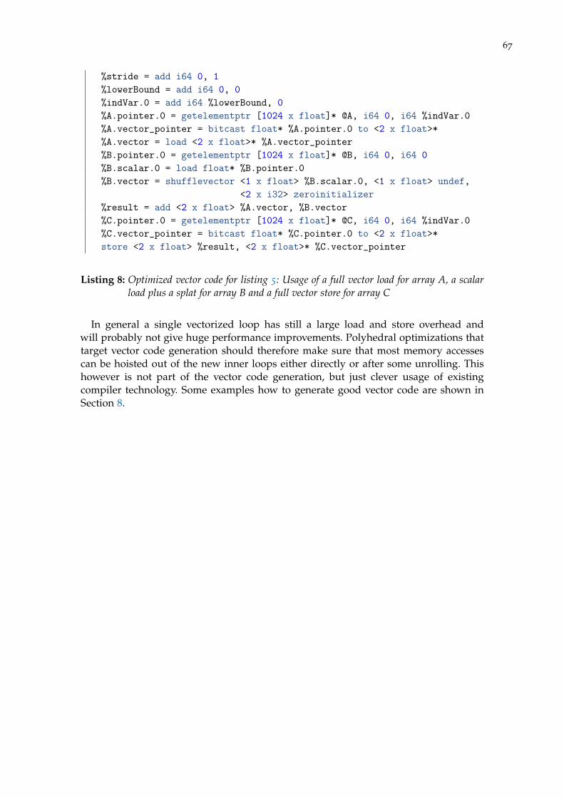
67

%stride = add i64 0, 1%lowerBound = add i64 0, 0%indVar.0 = add i64 %lowerBound, 0%A.pointer.0 = getelementptr [1024 x float]* @A, i64 0, i64 %indVar.0%A.vector_pointer = bitcast float* %A.pointer.0 to <2 x float>*%A.vector = load <2 x float>* %A.vector_pointer%B.pointer.0 = getelementptr [1024 x float]* @B, i64 0, i64 0%B.scalar.0 = load float* %B.pointer.0%B.vector = shufflevector <1 x float> %B.scalar.0, <1 x float> undef,

<2 x i32> zeroinitializer%result = add <2 x float> %A.vector, %B.vector%C.pointer.0 = getelementptr [1024 x float]* @C, i64 0, i64 %indVar.0%C.vector_pointer = bitcast float* %C.pointer.0 to <2 x float>*store <2 x float> %result, <2 x float>* %C.vector_pointer

Listing 8: Optimized vector code for listing 5: Usage of a full vector load for array A, a scalarload plus a splat for array B and a full vector store for array C

In general a single vectorized loop has still a large load and store overhead andwill probably not give huge performance improvements. Polyhedral optimizations thattarget vector code generation should therefore make sure that most memory accessescan be hoisted out of the new inner loops either directly or after some unrolling. Thishowever is not part of the vector code generation, but just clever usage of existingcompiler technology. Some examples how to generate good vector code are shown inSection 8.

Part III

E X P E R I M E N T S

8M AT R I X M U LT I P L I C AT I O N - V E C T O R I Z E D

Matrix multiplication is a well known computation kernel, not just because of its simplestructure, but especially because of its importance as a building block of many complexalgorithms. To obtain good performance an optimized version of the matrix multipli-cation kernel is crucial. Such a kernel can be obtained by linking with special linearalgebra libraries like BLAS [18] or their vendor optimized counterparts. Yet, a more con-venient approach is to rely on the compiler to optimize such kernels automatically. Byanalyzing and optimizing a challenging variant of matrix multiplication we show whatimprovements are still possible over current compilers.

Listing 9 shows a plain matrix multiplication kernel that multiplies two 32x32 matri-ces and adds the obtained result to a third matrix. The kernel is not optimized in termsof vector intrinsics or any special loop structure, but a competitive compiler should cre-ate such a loop structure automatically. For the shown kernel this is not straightforward,as all memory accesses have unit stride in respect to different loop dimensions. If theloop nest is vectorized along one dimension only one memory access has unit stride,whereas the other two memory accesses will have non unit strides. With clever use ofunrolling, loop interchange and strip mining, the cost of those non-unit stride accessescan be reduced, such that the use of SIMD instructions becomes profitable.

void matmul(float *restrict A, float *restrict B, float *restrict C) {for (i=0; i < 32; i++)

for (j=0; j < 32; j++)for (k=0; k < 32; k++)

C[i][j] += A[k][i] * B[j][k];}

Listing 9: Matrix multiplication kernel where each memory access has a unit stride in respectto another loop dimension

Figure 23 shows the performance of this kernel with the different steps that can betaken to optimize code with Polly. The baseline is LLVM with all optimizations enabled,which is equivalent to the use of clang -O3. At version 2.8 LLVM does not change theloop structure of the kernel at all and no SIMD instructions are created. Even if LLVMdoes not apply neither vectorization nor memory access optimizations, good scalar code

71

72

is created. GCC 4.4.5 does also not apply any loop transformations nor does it applyany vectorization. The performance of the GCC generated code shows that its scalarcode is not as good as the code created by LLVM. In contrast ICC 11.1 performs looptransformations and introduces SIMD instructions. The code it generates is almost twiceas fast as the one generated with LLVM. Yet, the assembly of the ICC generated codecontains a large amount of scalar loads, which suggests that further optimization arepossible.

Now Polly is used to generate optimized vector code. We lower the kernel to LLVM-IRand execute the Polly optimizations on it. After Polly’s code generation the LLVM stan-dard optimizations are scheduled to remove redundant scalar operations introduced byPolly. The first run shown is the Polly identity transformation which translates the ker-nel into the polyhedral model and recreates the LLVM-IR from the polyhedral represen-tation without applying any transformations. This example shows, that the indirectionthrough Polly does not add any notable overhead. The run time of the generated codedoes not increase.

for (k=0; k < 32; k++)for (j=0; j < 32; j+=4)

for (i=0; i < 32; i++)for (jj=j; jj < j + 4; j++)

C[i][jj] += A[k][i] * B[jj][k];

Listing 10: Matrix multiplication kernel with loop structure prepared for vectorization

The first transformation with Polly (+StripMine) changes the loop structure to im-prove data-locality and, more important, to expose a trivially vectorizable loop. Wederive the structure of the new loop nest with the help of a research tool developedby Stock et al. [44]. The abstract description of the loop structure is translated into apolyhedral schedule and this schedule is manually imported into Polly. As can be seenin Listing 10 an innermost trivially vectorizable jj loop is generated. In addition the iloop is moved deeper into the loop structure, a transformation that later enables furtheroptimizations. Even the simple change of the loop structure increases the performanceby 19%.

for (k=0; k < 32; k++)for (j=0; j < 32; j+=4)

for (i=0; i < 32; i++)C[i][j:j+3] += A[k][i] * B[j:3][k];

Listing 11: Vectorized matrix multiplication kernel

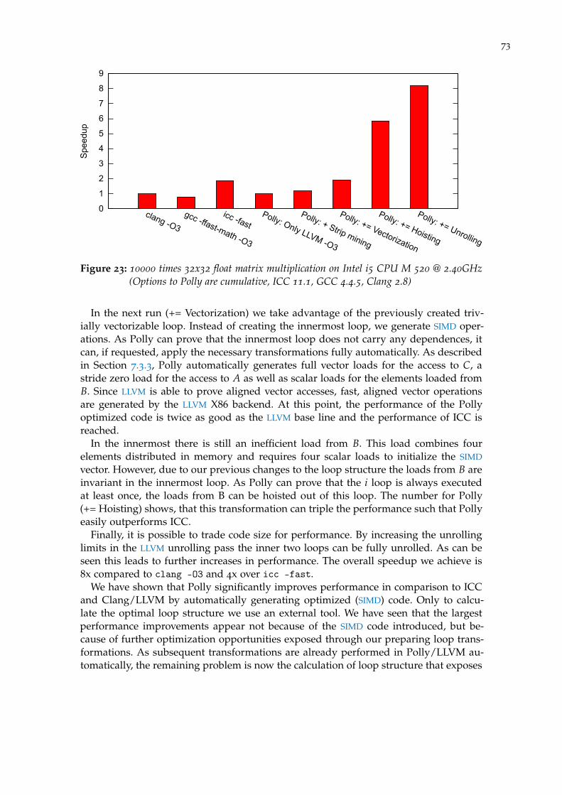
73

0

1

2

3

4

5

6

7

8

9

clang -O3

gcc -ffast-math -O3

icc -fastPolly: Only LLVM -O3

Polly: + Strip mining

Polly: += Vectorization

Polly: += Hoisting

Polly: += Unrolling

Spe

edup

Figure 23: 10000 times 32x32 float matrix multiplication on Intel i5 CPU M 520 @ 2.40GHz(Options to Polly are cumulative, ICC 11.1, GCC 4.4.5, Clang 2.8)

In the next run (+= Vectorization) we take advantage of the previously created triv-ially vectorizable loop. Instead of creating the innermost loop, we generate SIMD oper-ations. As Polly can prove that the innermost loop does not carry any dependences, itcan, if requested, apply the necessary transformations fully automatically. As describedin Section 7.3.3, Polly automatically generates full vector loads for the access to C, astride zero load for the access to A as well as scalar loads for the elements loaded fromB. Since LLVM is able to prove aligned vector accesses, fast, aligned vector operationsare generated by the LLVM X86 backend. At this point, the performance of the Pollyoptimized code is twice as good as the LLVM base line and the performance of ICC isreached.

In the innermost there is still an inefficient load from B. This load combines fourelements distributed in memory and requires four scalar loads to initialize the SIMDvector. However, due to our previous changes to the loop structure the loads from B areinvariant in the innermost loop. As Polly can prove that the i loop is always executedat least once, the loads from B can be hoisted out of this loop. The number for Polly(+= Hoisting) shows, that this transformation can triple the performance such that Pollyeasily outperforms ICC.

Finally, it is possible to trade code size for performance. By increasing the unrollinglimits in the LLVM unrolling pass the inner two loops can be fully unrolled. As can beseen this leads to further increases in performance. The overall speedup we achieve is8x compared to clang -O3 and 4x over icc -fast.

We have shown that Polly significantly improves performance in comparison to ICCand Clang/LLVM by automatically generating optimized (SIMD) code. Only to calcu-late the optimal loop structure we use an external tool. We have seen that the largestperformance improvements appear not because of the SIMD code introduced, but be-cause of further optimization opportunities exposed through our preparing loop trans-formations. As subsequent transformations are already performed in Polly/LLVM au-tomatically, the remaining problem is now the calculation of loop structure that exposes

74

sufficient optimization opportunities. The polyhedral abstractions provide a powerfulinstrument to target this problem.

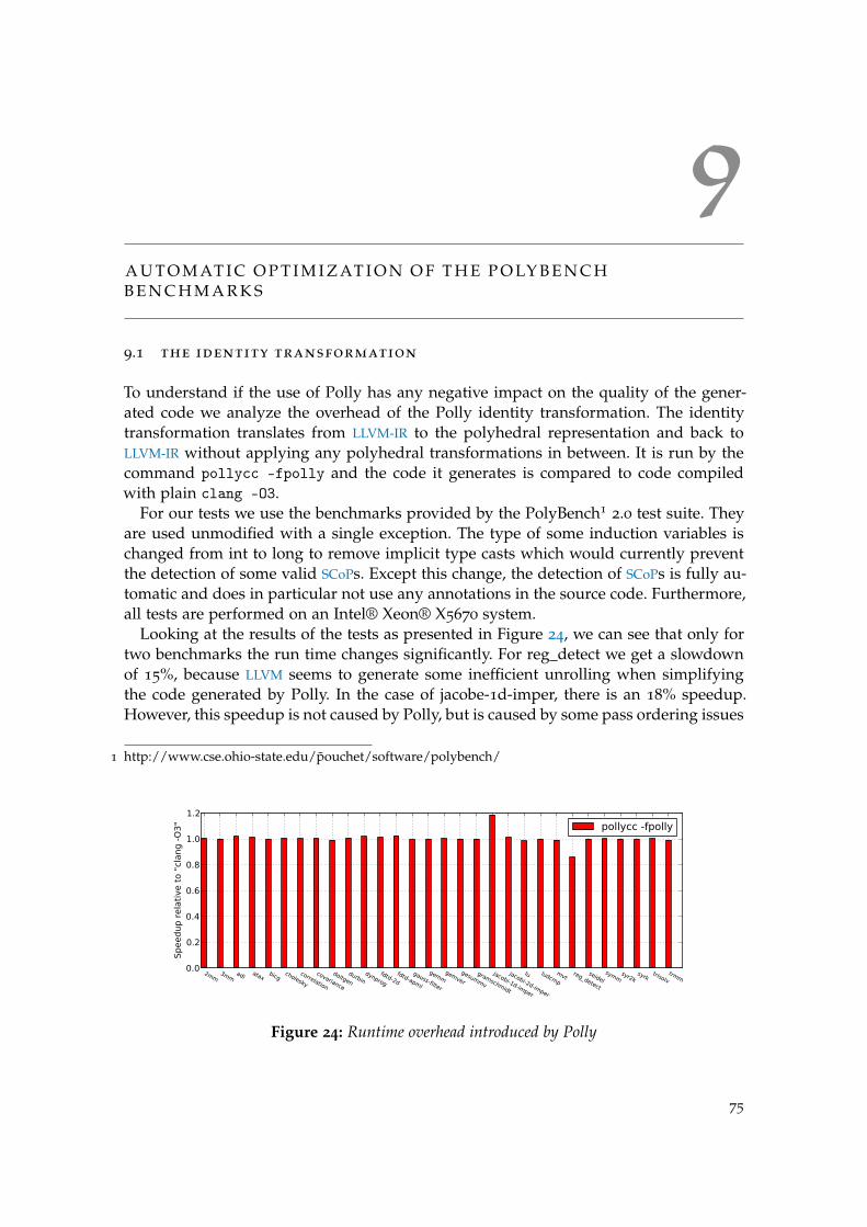
9A U T O M AT I C O P T I M I Z AT I O N O F T H E P O LY B E N C HB E N C H M A R K S

9.1 the identity transformation

To understand if the use of Polly has any negative impact on the quality of the gener-ated code we analyze the overhead of the Polly identity transformation. The identitytransformation translates from LLVM-IR to the polyhedral representation and back toLLVM-IR without applying any polyhedral transformations in between. It is run by thecommand pollycc -fpolly and the code it generates is compared to code compiledwith plain clang -O3.

For our tests we use the benchmarks provided by the PolyBench12.0 test suite. They

are used unmodified with a single exception. The type of some induction variables ischanged from int to long to remove implicit type casts which would currently preventthe detection of some valid SCoPs. Except this change, the detection of SCoPs is fully au-tomatic and does in particular not use any annotations in the source code. Furthermore,all tests are performed on an Intel® Xeon® X5670 system.

Looking at the results of the tests as presented in Figure 24, we can see that only fortwo benchmarks the run time changes significantly. For reg_detect we get a slowdownof 15%, because LLVM seems to generate some inefficient unrolling when simplifyingthe code generated by Polly. In the case of jacobe-1d-imper, there is an 18% speedup.However, this speedup is not caused by Polly, but is caused by some pass ordering issues

1 http://www.cse.ohio-state.edu/p̃ouchet/software/polybench/

2mm3mm

adiatax

bicgcholesky

correlation

covariance

doitgen

durbindynprog

fdtd-2d

fdtd-apml

gauss-filter

gemmgemver

gesummv

gramschmidt

jacobi-1d-imper

jacobi-2d-imper

lu ludcmp

mvtreg_detect

seidel

symmsyr2k

syrktrisolv

trmm0.0

0.2

0.4

0.6

0.8

1.0

1.2

Speedup r

ela

tive t

o "

clang -

O3" pollycc -fpolly

Figure 24: Runtime overhead introduced by Polly

75

76

2mm3mm

adiatax

bicgcholesky

correlation

covariance

doitgen

durbindynprog

fdtd-2d

fdtd-apml

gauss-filter

gemmgemver

gesummv

gramschmidt

jacobi-1d-imper

jacobi-2d-imper

lu ludcmp

mvtreg_detect

seidel

symmsyr2k

syrktrisolv

trmm0

1

2

3

4

5Speedup r

ela

tive t

o "

clang -

O3

" clang -O3pollycc -ftilepollycc -ftile -fvector

(a) Small data size

2mm3mm

adiatax

bicgcholesky

correlation

covariance

doitgen

durbindynprog

fdtd-2d

fdtd-apml

gauss-filter

gemmgemver

gesummv

gramschmidt

jacobi-1d-imper

jacobi-2d-imper

lu ludcmp

mvtreg_detect

seidel

symmsyr2k

syrktrisolv

trmm0

2

4

6

8

10

12

14

16

Speedup r

ela

tive t

o "

clang -

O3

" clang -O3pollycc -ftilepollycc -ftile -fvector

(b) Large data size

Figure 25: Sequential speedup of pollycc compared to clang (Both current from 25/03/2011,Benchmark: Polybench 2.0, run on Intel® Core™ Xeon X5670 CPU @ 2.93GHz)

in LLVM. Those issues are hidden, if the LLVM standard optimization passes are run asecond time to clean up the LLVM-IR produced by the Polly code generation. Except ofthese two cases, all other 28 benchmarks show performance changes of less than 2%and on average a run time increase of less than 0.4%. This shows clearly, that the use ofPolly does in most cases not introduce significant overhead.

9.2 creating optimized sequential code with pluto

To investigate the benefits fully automatic optimizations can currently provide for singlethread performance we connect Polly with PoCC2 and test the benefits of Pluto basedtiling and vectorization. Even though Pluto based tiling is focusing on parallel perfor-mance, it can already give a first impression what polyhedral optimizations can achieve.Our tests were run again on the PolyBench 2.0 test suite on an Intel® Xeon® X5670

2 PoCC-rc3.1 as available from http://www.cse.ohio-state.edu/~pouchet/software/pocc/

77

system. All tests are run with double precision floating point numbers on both smalland larger data sizes.

The test results presented in Figure 25a show 7 benchmarks, where tiling decreasesthe performance. Those are most of the time benchmarks, where tiling is not beneficialin general or where the problem size is too small to benefit from tiling. Due to the intro-duction of more complex control flow, the run time of those test cases increases. This isexpected, as Polly currently does not include a heuristic to determine, if the use tilingwill be profitable. For 9 of 30 benchmarks, Pluto based tiling can provide significantperformance improvements even on small data sizes. For larger data sizes we obtain inaverage 2x speedup with 4 benchmarks showing more than 4x speedup and two evenreaching 8x speedup. This is promising, as we have not yet analyzed the benchmarksintensively and the calculated schedules are most probably not yet optimal. Lookingat the SIMD code generation we see that for two cases Pluto based vectorization canfurther increase the speedup. This is for example the case for gemm where additionaluse of vector operations leads to an overall speedup of 14x. To emphasize, this is stillsingle thread performance and the speedup is only obtained by a more efficient use ofcaches and SIMD units. We also see that in many cases vectorization actually decreasesthe performance of the code. The reason here is that Pluto currently does not includeany useful heuristics to decide how to vectorize, but always vectorizes the innermostparallel loop. In case this loop has no stride one accesses, the vectorization of this loopis often not beneficial. We believe, that by developing better heuristics for vectorization,benefits as seen for gemm can be shown for more benchmarks.

9.3 creating optimized parallel code with pluto

We also analyze the performance benefits that we can obtain by generating OpenMPparallel code. For this we start with tiling and vectorization. Then, we use Pluto’s par-allel mode to expose parallelism and we use Polly to create OpenMP code that takesadvantage of this parallelism. All tests were run on a 2 socket, 12 core, 24 HT3 threadsIntel® Xeon® X5670 system.

As can be seen in Figure 26, 16 of 30 benchmarks benefit from parallel execution.Even with small data sizes 8 benchmarks reach more than 10x speedup. For larger datasizes we obtain in average 12x speedup and there exist even a case that shows morethan 80x speedup. We believe this already shows clearly that there exists a larger setof benchmarks that benefit from automatic parallelization as it can be performed inPolly. Together with vectorization, the gemm kernel is again the top performer with anoverall speedup of more than 100x. As can be seen, parallelism combined with tilingand vectorization can show significant performance improvements for a large numberof benchmarks. And again, we did not yet optimize the tests intensively such that weexpect further improvements. The limited benefits vectorization currently provides sug-gest another area where further performance improvements may be possible.

3 HyperThreading

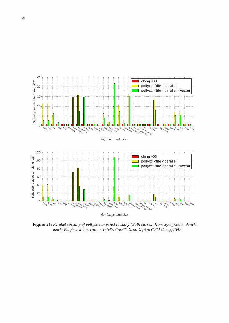
78

2mm3mm

adiatax

bicgcholesky

correlation

covariance

doitgen

durbindynprog

fdtd-2d

fdtd-apml

gauss-filter

gemmgemver

gesummv

gramschmidt

jacobi-1d-imper

jacobi-2d-imper

lu ludcmp

mvtreg_detect

seidel

symmsyr2k

syrktrisolv

trmm0

5

10

15

20

25

Speedup r

ela

tive t

o "

clang -

O3

" clang -O3pollycc -ftile -fparallelpollycc -ftile -fparallel -fvector

(a) Small data size

2mm3mm

adiatax

bicgcholesky

correlation

covariance

doitgen

durbindynprog

fdtd-2d

fdtd-apml

gauss-filter

gemmgemver

gesummv

gramschmidt

jacobi-1d-imper

jacobi-2d-imper

lu ludcmp

mvtreg_detect

seidel

symmsyr2k

syrktrisolv

trmm0

20

40

60

80

100

120

Speedup r

ela

tive t

o "

clang -

O3

" clang -O3pollycc -ftile -fparallelpollycc -ftile -fparallel -fvector

(b) Large data size

Figure 26: Parallel speedup of pollycc compared to clang (Both current from 25/03/2011, Bench-mark: Polybench 2.0, run on Intel® Core™ Xeon X5670 CPU @ 2.93GHz)

10C O N C L U S I O N

In this thesis we presented Polly, a framework to apply polyhedral transformations ona low level intermediate representation. We have shown how to automatically extractthe static control parts of a program, how to translate them into a polyhedral descrip-tion, how to apply transformations on this description and finally, how to regenerateoptimized program code. The process described is programming language independentand does not require the input code to follow any syntactical form. Instead, we analyzea program semantically such that different textual incarnations of semantically equiv-alent constructs are supported transparently. As a result, code that contains constructslike goto-loops or pointer arithmetic can be optimized.

To represent the code Polly uses a modern polyhedral description based on an inte-ger set library with support for a detailed data-flow analysis. This analysis is used todetect different forms of parallelism. For outermost parallel loops we introduce calls toan OpenMP runtime and in case of innermost parallel loops we create SIMD code. For thegenerated SIMD code we automatically determine the optimal vector instructions, suchthat polyhedral optimizers can focus on finding an execution order that exposes op-portunities for generating effective vector code. Furthermore, we have defined a genericinterface for external optimizers. It was used to connect PoCC,1 a collection of polyhedraltools which includes the advanced data-locality and parallelism optimizer Pluto.

To understand the effectiveness of Polly, we optimized the Polybench 2.0 test suite andanalyzed the results. The indirection through the polyhedral representation does notintroduce any overhead in the generated code. In case the Pluto optimizations are used,we have seen significant speedups that reached 14x without introducing thread levelparallelism and more than 100x when taking advantage of thread level parallelism.2

In average we reached a 2x speedup without and a 12x speedup with thread levelparallelism.3 As the focus of this work was more on the infrastructure than on theoptimizer, we believe these numbers can be further improved.

At this stage, we have finished the core of Polly, but to optimize code that commonlyappears in larger applications further extensions are necessary. The main areas thatneed work are type cast operations, possible integer overflows and multi-dimensionalvariable sized arrays (multi-dimensional arrays with static size are already supported).Furthermore, we have seen that Pluto does not yet produce loop nests that allow effec-tive SIMD code generation, such that currently only manually calculated optimizationsshow the benefits of our SIMD back end. Work to extend the Pluto algorithm to expose

1 http://pocc.sf.net2 For the gemm kernel and large data size3 For large data sizes

79

80

better SIMD code generation opportunities is planned. Another topic that we plan totarget is the support for memory layout transformations.

Polly can apply advanced, polyhedral transformations without the need of any sourcecode annotations or the use of source-to-source techniques. As it works directly insidea compiler, it can be used to optimize existing programs fully automatically. We havealready shown significant performance improvements on a number of computation ker-nels with the help of the Pluto optimizers and believe that the Polly infrastructure willsimplify the development of new, advanced optimizations. As it abstracts away all lan-guage specific details and code generation problems, it allows to focus on the high-leveloptimization problems. With the interface for external optimizers new transformationscan be added to Polly without the need to understand all LLVM internals. Open re-search topics that may benefit from Polly are for example polyhedral optimizations injust-in-time environments, automatic offloading of calculations to vector accelerators orpolyhedral optimizations in high level synthesis. As LLVM provides a good infrastruc-ture for these topics,4 even solutions that target several of these problems at once couldbe investigated.

4 In LLVM provides a JIT compiler as well as PTX and Verilog code generation.

Part IV

A P P E N D I X

L I S T O F F I G U R E S

Figure 1 Static compilation using the llvm toolchain . . . . . . . . . . . . . . 8

Figure 2 CFG of the example program . . . . . . . . . . . . . . . . . . . . . . 14

Figure 3 The dominator tree for the CFG in Figure 2 . . . . . . . . . . . . . . 15

Figure 4 A simple Region . . . . . . . . . . . . . . . . . . . . . . . . . . . . . 16

Figure 5 Transform a refined region to a simple region . . . . . . . . . . . . 17

Figure 6 Simple (solid border) and refined (dashed border) regions in a CFG. 17

Figure 7 The elements of a scalar evolution . . . . . . . . . . . . . . . . . . . 19

Figure 8 A loop nest and the two basic sets used to describe the valid loopiterations. . . . . . . . . . . . . . . . . . . . . . . . . . . . . . . . . . 24

Figure 9 Architecture of Polly . . . . . . . . . . . . . . . . . . . . . . . . . . . 30

Figure 10 Passes available in Polly as printed by ’opt -load LLVMPolly.so-help’ . . . . . . . . . . . . . . . . . . . . . . . . . . . . . . . . . . . . 31

Figure 11 pollycc command line options . . . . . . . . . . . . . . . . . . . . . 32

Figure 12 A valid SCoP (validity defined on ASTs) . . . . . . . . . . . . . . . . 34

Figure 13 Two valid SCoPs (validity defined based on semantics) and theircanonical counterparts . . . . . . . . . . . . . . . . . . . . . . . . . . 35

Figure 14 An example of a SCoP and its polyhedral representation. . . . . . . 38

Figure 15 Translation from C over LLVM-IR to polyhedral shown on a sim-ple example . . . . . . . . . . . . . . . . . . . . . . . . . . . . . . . . 41

Figure 16 Region based SCoP detection . . . . . . . . . . . . . . . . . . . . . . 42

Figure 17 Simple SCoP before independent block pass . . . . . . . . . . . . . 45

Figure 18 Simple SCoP after independent block pass . . . . . . . . . . . . . . 46

Figure 19 JSCoP file of a matrix multiplication kernel . . . . . . . . . . . . . . 53

Figure 20 MayWrites and accesses to memory ranges . . . . . . . . . . . . . . 56

Figure 21 Three kinds of vector loads: v1 is a stride-one vector load, v2 is astride-zero vector load and v3 is a complex vector load . . . . . . . 65

Figure 22 Two kind of vector stores: v1 is a stride-one vector store and v3 isa complex vector store . . . . . . . . . . . . . . . . . . . . . . . . . . 65

Figure 23 10000 times 32x32 float matrix multiplication on Intel i5 CPU M520 @ 2.40GHz (Options to Polly are cumulative, ICC 11.1, GCC4.4.5, Clang 2.8) . . . . . . . . . . . . . . . . . . . . . . . . . . . . . . 73

Figure 24 Runtime overhead introduced by Polly . . . . . . . . . . . . . . . . 75

Figure 25 Sequential speedup of pollycc compared to clang (Both currentfrom 25/03/2011, Benchmark: Polybench 2.0, run on Intel® Core™Xeon X5670 CPU @ 2.93GHz) . . . . . . . . . . . . . . . . . . . . . . 76

83

84

Figure 26 Parallel speedup of pollycc compared to clang (Both current from25/03/2011, Benchmark: Polybench 2.0, run on Intel® Core™ XeonX5670 CPU @ 2.93GHz) . . . . . . . . . . . . . . . . . . . . . . . . . 78

L I S T O F TA B L E S

85

L I S T O F L I S T I N G S

1 Two different ASTs generated from the same SCoP. . . . . . . . . . . . . . . 58

2 A single loop nest hides parallelism . . . . . . . . . . . . . . . . . . . . . . 60

3 Two separate loop nests expose parallelism . . . . . . . . . . . . . . . . . . 60

4 Two steps to vectorize a loop . . . . . . . . . . . . . . . . . . . . . . . . . . 64

5 Example of a trivially vectorizable loop . . . . . . . . . . . . . . . . . . . . 64

6 The LLVM-IR of the loop body in listing 5 . . . . . . . . . . . . . . . . . . 65

7 Unoptimized vector code for listing 5 . . . . . . . . . . . . . . . . . . . . . 66

8 Optimized vector code for listing 5: Usage of a full vector load for arrayA, a scalar load plus a splat for array B and a full vector store for array C 67

9 Matrix multiplication kernel where each memory access has a unit stridein respect to another loop dimension . . . . . . . . . . . . . . . . . . . . . . 71

10 Matrix multiplication kernel with loop structure prepared for vectorization 72

11 Vectorized matrix multiplication kernel . . . . . . . . . . . . . . . . . . . . 72

86

L I S T O F A C R O N Y M S

VMaIR

ast Abstract Syntax Tree

blas Basic Linear Algebra Subprogram

cfg Control Flow Graph

cloog Chunky Loop Generator

cisc Complex instruction set computing

gcc GNU Compiler Collection

ghc Glasgow Haskell Compiler

gpgpu General-purpose computing on graphics processing units

hls High Level Synthesis

isl integer set library

jscop JSON SCoP

json JavaScript Object Notation

llvm Low Level Virtual Machine

llvm-ir LLVM Intermediate Representation

openmp Open Multi-Processing

pocc Polyhedral Compilation Collection

scop Static Control Part

ssa Static Single Assignment

simd Single Instruction Multiple Data

87

R E F E R E N C E S

[1] DragonEgg. http://dragonegg.llvm.org/, 2010.

[2] Icedtea. http://icedtea.classpath.org/, 2010.

[3] LLVM Lua. http://code.google.com/p/llvm-lua/, 2010.

[4] LLVM’s Analysis and Transform Passes. http://llvm.org/docs/Passes.html,2011.

[5] LLVM Ruby. http://www.llvmruby.org/, 2010.

[6] Unladen Swallow. http://code.google.com/p/unladen-swallow/, 2010.

[7] A. V. Aho, M. S. Lam, R. Sethi, and J. D. Ullman. Compilers: Principles, Techniques,and Tools (2nd Edition). Addison-Wesley, Aug. 2006.

[8] O. Bachmann, P. S. Wang, and E. V. Zima. Chains of Recurrences - A Method toExpedite the Evaluation of Closed-form Functions. In Proceedings of the InternationalSymposium on Symbolic and Algebraic Computation, ISSAC ’94, pages 242–249. ACM,1994.

[9] S. Baghdadi, A. Größlinger, and A. Cohen. Putting Automatic Polyhedral Compila-tion for GPGPU to Work. In Proceedings of the 15th Workshop on Compilers for ParallelComputers (CPC’10), jul 2010.

[10] M. Baskaran, J. Ramanujam, and P. Sadayappan. Automatic C-to-CUDA CodeGeneration for Affine Programs. In Compiler Construction, volume 6011 of LectureNotes in Computer Science, pages 244–263. Springer Berlin / Heidelberg, 2010.

[11] C. Bastoul. Code Generation in the Polyhedral Model is Easier Than You Think. InPACT’13 IEEE International Conference on Parallel Architecture and Compilation Tech-niques, pages 7–16, Sept. 2004.

[12] M.-W. Benabderrahmane, L.-N. Pouchet, A. Cohen, and C. Bastoul. The Polyhe-dral Model is More Widely Applicable Than You Think. . In ETAPS InternationalConference on Compiler Construction (CC’2010), pages 283–303. Springer Verlag, Mar.2010.

[13] U. Bondhugula, A. Hartono, J. Ramanujam, and P. Sadayappan. A Practical Auto-matic Polyhedral Parallelizer and Locality Optimizer. In Proceedings of the 2008ACM SIGPLAN Conference On Programming Language Design and Implementation,PLDI ’08, pages 101–113. ACM, 2008.

89

90

[14] A. Canis, J. Choi, M. Aldham, V. Zhang, A. Kammoona, J. Anderson, S. Brown,and T. Czajkowski. LegUp: High-Level Synthesis for FPGA-Based Proces-sor/Accelerator Systems. In Proceedings of the 19th Annual ACM/SIGDA InternationalSymposium on Field Programmable Gate Arrays, FPGA ’11, 2011.

[15] C. Chen, J. Chame, and M. Hall. CHiLL: A Framework for Composing High-LevelLoop Transformations. Technical Report 08-897, June 2008.

[16] P. Clauss and B. Meister. Automatic Memory Layout Transformations to OptimizeSpatial Locality in Parameterized Loop Nests. SIGARCH Computer ArchitectureNews, 28:11–19, Mar. 2000.

[17] D. Crockford. The application/json Media Type for JavaScript Object Notation(JSON). RFC 4627 (Informational), July 2006. URL http://www.ietf.org/rfc/rfc4627.txt.

[18] J. Dongarra. Preface: Basic Linear Algebra Subprograms Technical (Blast) ForumStandard. International Journal of High Performance Computing Applications, 16:1,February 2002.

[19] R. A. V. Engelen. Efficient Symbolic Analysis for Optimizing Compilers. In InProceedings of the International Conference on Compiler Construction, ETAPS CC ’O1,pages 118–132, 2001.

[20] P. Feautrier. Dataflow analysis of array and scalar references. 20:23–53, 1991.

[21] P. Feautrier. Automatic Parallelization in the Polytope Model. In G.-R. Perrin andA. Darte, editors, The Data Parallel Programming Model, volume 1132 of Lecture Notesin Computer Science, pages 79–103. Springer Berlin / Heidelberg, 1996.

[22] Free Software Foundation Inc. Welcome to the Home of GOMP. http://gcc.gnu.org/projects/gomp/, 2010.

[23] S. Girbal, N. Vasilache, C. Bastoul, A. Cohen, D. Parello, M. Sigler, and O. Temam.Semi-automatic Composition of Loop Transformations For Deep Parallelism andMemory Hierarchies. International Journal of Parallel Programming, 34:261–317, 2006.

[24] M. Griebl and C. Lengauer. The Loop Parallelizer LooPo. In Languages and Compil-ers for Parallel Computing, volume 1239 of Lecture Notes in Computer Science, pages603–604. Springer Berlin / Heidelberg, 1997.

[25] M. Griebl, P. Feautrier, and C. Lengauer. Index Set Splitting. International Journal ofParallel Programming, 28:607–631, 2000.

[26] G. Gupta and S. Rajopadhye. The Z-polyhedral model. In Proceedings of the 12thACM SIGPLAN Symposium on Principles and Practice of Parallel Programming, PPoPP’07, pages 237–248, 2007.

[27] R. Johnson, D. Pearson, and K. Pingali. The Program Structure Tree: ComputingControl Regions in Linear Time. In Proceedings of the ACM SIGPLAN 1994 Conferenceon Programming Language Design and Implementation, PLDI ’94, pages 171–185. ACM,1994.

91

[28] M. Kandemir, A. Choudhary, N. Shenoy, P. Banerjee, and J. Ramanujam. A Hy-perplane Based Approach for Optimizing Spatial Locality in Loop Nests. In Pro-ceedings of the 12th international conference on Supercomputing, ICS ’98, pages 69–76.ACM, 1998.

[29] W. Kelly and W. Pugh. A Unifying Framework for Iteration Reordering Transfor-mations. In Algorithms and Architectures for Parallel Processing, 1995. ICAPP 95. IEEEFirst ICA/sup 3/PP., volume 1, pages 153 –162 vol.1, Apr. 1995.

[30] C. Lattner. LLVM Language Reference Manual. http://llvm.org/docs/LangRef.html.

[31] C. Lattner and V. Adve. LLVM: A Compilation Framework for Lifelong ProgramAnalysis & Transformation. In Proceedings of the 2004 International Symposium onCode Generation and Optimization (CGO’04), Mar 2004.

[32] M. Levoy. Experimental platforms for computational photography. IEEE ComputerGraphics and Applications, 30:81–87, 2010.

[33] LLVM Project. Developer Meeting 2010. http://llvm.org/devmtg/2010-11/, 2010.

[34] LLVM Project. Users of LLVM. http://llvm.org/Users.html, 2010.

[35] TIOBE Software BV. TIOBE Programming Community Index. http://www.tiobe.com/index.php/content/paperinfo/tpci/index.html, Jan. 2011.

[36] M. Perache, H. Jourdren, and R. Namyst. MPC: A Unified Parallel Runtime forClusters of NUMA Machines. In Euro-Par 2008 - Parallel Processing, volume 5168 ofLecture Notes in Computer Science, pages 78–88. Springer Berlin / Heidelberg, 2008.

[37] S. Pop. Analysis of Induction Variables Using Chains of Recurrences: Extensions.Master’s thesis, Universite Louis Pasteur, Strasbourg, 2003.

[38] R. T. Prosser. Applications of Boolean Matrices to the Analysis of Flow Diagrams.In IRE-AIEE-ACM ’59 (Eastern): Papers presented at the December 1-3, 1959, easternjoint IRE-AIEE-ACM computer conference, pages 133–138. ACM, 1959.

[39] W. Pugh and D. Wonnacott. An exact method for analysis of value-based arraydata dependences. In U. Banerjee, D. Gelernter, A. Nicolau, and D. Padua, edi-tors, Languages and Compilers for Parallel Computing, volume 768 of Lecture Notes inComputer Science, pages 546–566. 1994.

[40] A. R. Putnam, D. Bennett, E. Dellinger, J. Mason, and P. Sundararajan. CHiMPS: AHigh-level Compilation Flow for Hybrid CPU-FPGA Architectures. In Proceedingsof the 16th International ACM/SIGDA symposium on Field Programmable Gate Arrays,FPGA ’08, pages 261–261. ACM, 2008.

[41] F. Quilleré, S. Rajopadhye, and D. Wilde. Generation of Efficient Nested Loopsfrom Polyhedra. International Journal on Parallel Programming, 28:469–498, October2000.

92

[42] S. Rajopadhye, L. Renghanarayana, G. Gupta, and M. M. Strout. Computations onIteration Spaces, chapter 15. CRC Press, second edition, 2008.

[43] T. Risset, S. Derrien, P. Quinton, and S. Rajopadhye. High-Level Synthesis of LoopsUsing the Polyhedral Model. In High-Level Synthesis : From Algorithm to DigitalCircuit, pages 215–230. 2008.

[44] K. Stock, T. Henretty, I. Murugandi, and P. Sadayappan. Model-Driven SIMD CodeGeneration for a Multi-Resolution Tensor Kernel. In IPDPS, 2011. Accepted forpublication.

[45] L. Tarrataca, A. C. Santos, and J. a. M. P. Cardoso. The Current Feasibility ofGesture Recognition for a Smartphone Using J2ME. In Proceedings of the 2009 ACMSymposium on Applied Computing, SAC ’09, pages 1642–1649. ACM, 2009.

[46] D. A. Terei and M. M. Chakravarty. An LLVM Backend for GHC. In Proceedingsof the Third ACM Haskell Symposium on Haskell, Haskell ’10, pages 109–120. ACM,2010.

[47] The mono project. Mono LLVM. http://icedtea.classpath.org/, 2010.

[48] K. Trifunovic, A. Cohen, D. Edelsohn, F. Li, T. Grosser, H. Jagasia, R. Ladelsky,S. Pop, J. Sjödin, and R. Upadrasta. GRAPHITE Two Years After: First LessonsLearned From Real-World Polyhedral Compilation. In GCC Research OpportunitiesWorkshop (GROW’10), jan 2010. URL http://hal.inria.fr/inria-00551516/en/.

[49] J. Vanhatalo, H. Völzer, and J. Koehler. The Refined Process Structure Tree. In BPM’08: Proceedings of the 6th International Conference on Business Process Management,pages 100–115. Springer-Verlag, 2008.

[50] S. Verdoolaege. ISL: An Integer Set Library for the Polyhedral Model. In Mathemat-ical Software - ICMS 2010, volume 6327 of Lecture Notes in Computer Science, pages299–302. Springer Berlin / Heidelberg, 2010.

[51] J. Villarreal, A. Park, W. Najjar, and R. Halstead. Designing Modular HardwareAccelerators in C with ROCCC 2.0. In Field-Programmable Custom Computing Ma-chines (FCCM), 2010 18th IEEE Annual International Symposium on, pages 127 –134,May 2010.

[52] D. Wagner, G. Reitmayr, A. Mulloni, T. Drummond, and D. Schmalstieg. Real-TimeDetection and Tracking for Augmented Reality on Mobile Phones. IEEE Transac-tions on Visualization and Computer Graphics, 16:355–368, 2010.

[53] Y.-C. Wang, S. Pang, and K.-T. Cheng. A GPU-accelerated Face Annotation Systemfor Smartphones. In Proceedings of the International Conference on Multimedia, MM’10, pages 1667–1668. ACM, 2010.

[54] R. P. Wilson, R. S. French, C. S. Wilson, S. P. Amarasinghe, J. M. Anderson, S. W. K.Tjiang, S. wei Liao, C. wen Tseng, M. W. Hall, M. S. Lam, and J. L. Hennessy. SUIF:An Infrastructure for Research on Parallelizing and Optimizing Compilers. ACMSIGPLAN Notices, 29:31–37, 1994.

93

[55] Y. Xiong and K. Pulli. Fast Panorama Stitching for High-quality Panoramic Imageson Mobile Phones. Consumer Electronics, IEEE Transactions on, 56:298 –306, May2010.

[56] B. Yee, D. Sehr, G. Dardyk, J. B. Chen, R. Muth, T. Ormandy, S. Okasaka, N. Narula,and N. Fullagar. Native Client: A Sandbox for Portable, Untrusted x86 Native Code.Security and Privacy, IEEE Symposium on, 0:79–93, 2009.

[57] J. Zhang, Z. Zhang, S. Zhou, M. Tan, X. Liu, X. Cheng, and J. Cong. Bit-level Op-timization for High-level Synthesis and FPGA-based Acceleration. In Proceedingsof the 18th annual ACM/SIGDA international symposium on Field programmable gatearrays, FPGA ’10, 2010.

[58] E. V. Zima. On Computational Properties of Chains of Recurrences. In Proceedingsof the 2001 international symposium on Symbolic and algebraic computation, ISSAC ’01,pages 345–. ACM, 2001.

D E C L A R AT I O N

Hiermit versichere ich, dass ich diese Diplomarbeit selbsständig und ohne Benutzunganderer als der angegebenen Quellen und Hilfsmittel angefertigt habe und alle Aus-führungen, die wörtlich oder sinngemäß übernommen wurden, als solche gekennzeich-net sind, sowie dass ich diese Diplomarbeit in gleicher oder ähnlicher Form noch keineranderen Prüfungsbehörde vorgelegt habe.

Passau, Germany, April 2011

Tobias Christian Grosser