introduction to automated polyhedral code optimizations and tiling
TRANSCRIPT

Introduction to Automated Polyhedral CodeOptimizations and Tiling
Alain Darte
CNRS, Compsys teamLaboratoire de l’Informatique du Parallélisme
École normale supérieure de Lyon
Spring School on Numerical Simulationand Polyhedral Code Optimizations
Saint Germain au Mont d’Or, May 10, 2016
1 / 98

Outline
1 Generalities
2 Polyhedral compilation
3 Classic loop transformations
4 Systems of uniform recurrence equations
5 Detection of loop parallelism
6 Kernel offloading and loop tiling
7 Inter-tile data reuse and local storage
2 / 98

GENERALITIES
3 / 98

Compiler: generalities
Interpreter
Input
data
Machine
Source
Program
Compiler
4 / 98

Compiler: generalities
Input
data
Machine
Source
Program
Compiler Target program
AoT vs JITStatic vs dynamicCross compilationParametric codesWorst-case opt. vsaverage-case opt.Language-specific ormulti-languageIntermediaterepresentations (IR)Runtime & libraries
4 / 98

Front-end and back-end
Front-endTarget independentSource-to-sourceHigh-level transf.Task & loop par.Memory opt.
Back-endTarget dependentInstr-level par. (ILP)PipeliningAVX, SIMD instr.SSA and registers
Figures from http://fr.slideshare.net/ssuser2cbb78/gcc-37841549.
5 / 98
Moore’s law and Dennard scaling
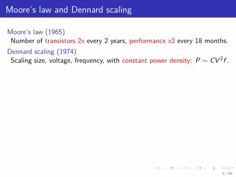
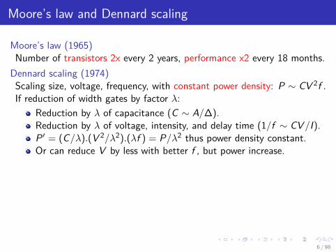
Moore’s law (1965)Number of transistors 2x every 2 years, performance x2 every 18 months.
Dennard scaling (1974)Scaling size, voltage, frequency, with constant power density: P ∼ CV 2f .
If reduction of width gates by factor λ:Reduction by λ of capacitance (C ∼ A/∆).Reduction by λ of voltage, intensity, and delay time (1/f ∼ CV /I).P ′ = (C/λ).(V 2/λ2).(λf ) = P/λ2 thus power density constant.Or can reduce V by less with better f , but power increase.
End of Dennard scaling f ∼ V − Vt (supply minus threshold voltage).But leakage power not negligible if Vt too small.
Frequency max around 2006 (∼ 4GHz).ILP, low-power CPU designs, multicore designs, GPUs.
* More burden on the programmers & compilers.
6 / 98
Moore’s law and Dennard scaling
Moore’s law (1965)Number of transistors 2x every 2 years, performance x2 every 18 months.
Dennard scaling (1974)Scaling size, voltage, frequency, with constant power density: P ∼ CV 2f .If reduction of width gates by factor λ:
Reduction by λ of capacitance (C ∼ A/∆).Reduction by λ of voltage, intensity, and delay time (1/f ∼ CV /I).P ′ = (C/λ).(V 2/λ2).(λf ) = P/λ2 thus power density constant.Or can reduce V by less with better f , but power increase.
End of Dennard scaling f ∼ V − Vt (supply minus threshold voltage).But leakage power not negligible if Vt too small.
Frequency max around 2006 (∼ 4GHz).ILP, low-power CPU designs, multicore designs, GPUs.
* More burden on the programmers & compilers.
6 / 98

The almost useless Amdahl’s law
See “A few bad ideas on the way to the triumph of parallel computing”, R. Schreiber, JPDC’14.
Amdahl’s law (1967)
Useless except to show what it does not consider
Tseq = sTseq + (1− s)Tseq, with s fraction not parallelizable.With p proc., Tpar/Tseq ≥ s + (1− s)/p ≥ s. Speed-up ≤ 1/s.
Simplistic view: correct formula in wrong model (∼ PRAM).Memory, comm., dedicated cores, program scaling, algorithmics!No insight even in favorable case, e.g., 2 independent purelysequential threads. Better: degree of parallelism, critical path, ratiocomm./computation, data locality (spatial & temporal), bandwidth.But: make sure single core perf. remains good in parallel implem.
Gustafson’s law Different reasoning, “scaling” programs.Tpar = sTpar + (1− s)Tpar, with s fraction of time in seq. core.With p proc., Tseq/Tpar ≥ s + (1− s)p. Speed-up ≥ (1− s)p.
7 / 98

The almost useless Amdahl’s law
See “A few bad ideas on the way to the triumph of parallel computing”, R. Schreiber, JPDC’14.
Amdahl’s law (1967) Useless except to show what it does not considerTseq = sTseq + (1− s)Tseq, with s fraction not parallelizable.With p proc., Tpar/Tseq ≥ s + (1− s)/p ≥ s. Speed-up ≤ 1/s.
Simplistic view: correct formula in wrong model (∼ PRAM).Memory, comm., dedicated cores, program scaling, algorithmics!No insight even in favorable case, e.g., 2 independent purelysequential threads. Better: degree of parallelism, critical path, ratiocomm./computation, data locality (spatial & temporal), bandwidth.But: make sure single core perf. remains good in parallel implem.
Gustafson’s law Different reasoning, “scaling” programs.Tpar = sTpar + (1− s)Tpar, with s fraction of time in seq. core.With p proc., Tseq/Tpar ≥ s + (1− s)p. Speed-up ≥ (1− s)p.
7 / 98

Where are we? HPC, embedded computing, accelerators
Performance increase how much is due to frequency increase, architectureimprovements, compilers, algorithm design?
Today’s complications Multi-level parallelism, memory hierarchy, bandwidthissues, attached accelerators, evolution in programming models.
Compiler challengesPPPP Programmability, performance, portability, productivity.Virtualization New IRs, Just-in-time (JIT) compilation, runtimes.Maintenance Retargetable compilers, cleaner designs.Predictability Architecture design, worst-case execution time (WCET).Certification Correct-by-construction, verification, certified compilers.Languages Domain-specific languages, parallel languages.
* New expectations, new compiler issues, but we can solve more.Automatic parallelization is irrealistic, but semi-automatic tools can help.
8 / 98

POLYHEDRAL COMPILATION
9 / 98

One view of history (borrowed from Steven Derrien)
Some actors of this evolution are here:P. Feautrier, P. Quinton, S. Rajopadhye, F. Irigoin, J. Ramanujam, A.Darte, A. Cohen, U. Bondhugula, S. Verdoolaege, T. Yuki, T. Grosser.
10 / 98

Multi-dimensional affine representation of loops and arrays
Matrix Multiplyint i,j,k;for(i = 0; i < n; i++)
for(j = 0; j < n; j++) S: C[i][j] = 0;
for(k = 0; k < n; k++) T: C[i][j] += A[i][k] * B[k][j];
iteration i
iteration j
Array C
Array B
Array A
iteration k
Instance-wise, element-wise, symbolic, parametric
Polyhedral Description Omega/ISCC syntax
So, that’s it?
Domain := [n]->S[i,j]: 0<=i,j<n; T[i,j,k]: 0<=i,j,k<n;
Read := [n]->T[i,j,k]->A[i,k]; T[i,j,k]->B[k,j]; T[i,j,k]->C[i,j];
Write := [n]->S[i,j]->C[i,j]; T[i,j,k]->C[i,j];
Order := [n]->S[i,j]->[i,j ,0]; T[i,j,k]->[i,j,1,k];
11 / 98

Multi-dimensional affine representation of loops and arrays
Matrix Multiplyint i,j,k;for(i = 0; i < n; i++)
for(j = 0; j < n; j++) S: C[i][j] = 0;
for(k = 0; k < n; k++) T: C[i][j] += A[i][k] * B[k][j];
iteration i
iteration j
Array C
Array B
Array A
iteration k
Instance-wise, element-wise, symbolic, parametric
Polyhedral Description Omega/ISCC syntax So, that’s it?Domain := [n]->S[i,j]: 0<=i,j<n; T[i,j,k]: 0<=i,j,k<n;
Read := [n]->T[i,j,k]->A[i,k]; T[i,j,k]->B[k,j]; T[i,j,k]->C[i,j];
Write := [n]->S[i,j]->C[i,j]; T[i,j,k]->C[i,j];
Order := [n]->S[i,j]->[i,j ,0]; T[i,j,k]->[i,j,1,k];
11 / 98

Ex: PPCG code for CPU+GPU, GPU part__global__ void kernel0(float *A, float *B, float *C, int n) /* n=12288 */
int b0 = blockIdx.y, b1 = blockIdx.x; /* Grid: 192x192 blocks, each with 32x32 threads */int t0 = threadIdx.y, t1 = threadIdx.x; /* Loops: 384x384x768 tiles, each with 32x32x16 points */__shared__ float shared_A[32][16]; /* Thus 1 block = 2x2x768 tiles, 1 thread = 1x1x16 points */__shared__ float shared_B[16][32];float private_C[1][1];
for (int g1 = 32 * b0; g1 <= 12256; g1 += 6144) /* 6144 = 32 (tile size) x 192 (number of blocks) */for (int g3 = 32 * b1; g3 <= 12256; g3 += 6144)
private_C[0][0] = C[(t0 + g1) * 12288 + (t1 + g3)];for (int g9 = 0; g9 <= 12272; g9 += 16) /* 16 consecutive points along k in a thread */
if (t0 <= 15) /* 32x32 threads, only 16x32 do the transfer */shared_B[t0][t1] = B[(t0 + g9) * 12288 + (t1 + g3)];
if (t1 <= 15) /* 32x32 threads, only 32x16 do the transfer */shared_A[t0][t1] = A[(t0 + g1) * 12288 + (t1 + g9)];
__syncthreads();for (int c4 = 0; c4 <= 15; c4 += 1) /* compute the 16 consecutive points along k */
private_C[0][0] += (shared_A[t0][c4] * shared_B[c4][t1]);__syncthreads();
C[(t0 + g1) * 12288 + (t1 + g3)] = private_C[0][0];__syncthreads();
PPCG compiler (Parkas)Verdoolaege, Cohen, etc.
12 / 98

Ex: PPCG code for CPU+GPU, GPU part (Volkov-like)__global__ void kernel0(float *A, float *B, float *C, int n) /* n=12288 */
int b0 = blockIdx.y, b1 = blockIdx.x; /* Grid: 192x192 blocks, each with 16x16 threads */int t0 = threadIdx.y, t1 = threadIdx.x; /* Loops: 384x384x768 tiles, each with 32x32x16 points */__shared__ float shared_A[32][16]; /* Thus 1 block = 2x2x768 tiles, 1 thread = 2x2x16 points */__shared__ float shared_B[16][32];float private_C[2][2];
for (int g1 = 32 * b0; g1 <= 12256; g1 += 6144) /* 6144 = 32 (tile size) x 192 (number of blocks) */for (int g3 = 32 * b1; g3 <= 12256; g3 += 6144)
private_C[0][0] = C[(t0 + g1) * 12288 + (t1 + g3)]; /* 2x2 points unrolled for register usage */private_C[0][1] = C[(t0 + g1) * 12288 + (t1 + g3 + 16)];private_C[1][0] = C[(t0 + g1 + 16) * 12288 + (t1 + g3)];private_C[1][1] = C[(t0 + g1 + 16) * 12288 + (t1 + g3 + 16)];for (int g9 = 0; g9 <= 12272; g9 += 16) /* 16 consecutive points along k in a thread */
for (int c1 = t1; c1 <= 31; c1 += 16) /* 16x32 to bring with 16x16 threads */shared_B[t0][c1] = B[(t0 + g9) * 12288 + (g3 + c1)];
for (int c0 = t0; c0 <= 31; c0 += 16) /* 32x16 to bring with 16x16 threads */shared_A[c0][t1] = A[(g1 + c0) * 12288 + (t1 + g9)];
__syncthreads();for (int c2 = 0; c2 <= 15; c2 += 1) /* unrolled for register usage */
private_C[0][0] += (shared_A[t0][c2] * shared_B[c2][t1]);private_C[0][1] += (shared_A[t0][c2] * shared_B[c2][t1 + 16]);private_C[1][0] += (shared_A[t0 + 16][c2] * shared_B[c2][t1]);private_C[1][1] += (shared_A[t0 + 16][c2] * shared_B[c2][t1 + 16]);
__syncthreads();
C[(t0 + g1) * 12288 + (t1 + g3)] = private_C[0][0];C[(t0 + g1) * 12288 + (t1 + g3 + 16)] = private_C[0][1];C[(t0 + g1 + 16) * 12288 + (t1 + g3)] = private_C[1][0];C[(t0 + g1 + 16) * 12288 + (t1 + g3 + 16)] = private_C[1][1];__syncthreads();
PPCG compiler (Parkas)Verdoolaege, Cohen, etc.
12 / 98

Typical criticism against polyhedral techniques
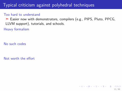
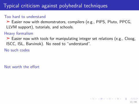
Too hard to understand
ã Easier now with demonstrators, compilers (e.g., PIPS, Pluto, PPCG,LLVM support), tutorials, and schools.
Heavy formalism
ã Easier now with tools for manipulating integer set relations (e.g., Cloog,ISCC, ISL, Barvinok). No need to “understand”.
No such codes
ã Not true for specific domains/architectures. But yes, extensions needed(e.g., approx., reconstruction, summaries, while loops).
Not worth the effort
ã Often the right limit for automation. Key for many analyses &optimizations, not just loop transformations. Growing industrial interest.
* Key to reason on multi-dimensional computations and data structures,and avoid explicit unrolling. More applications to come (e.g., looptermination, parallel languages, verification/certification, WCET).
13 / 98
Typical criticism against polyhedral techniques
Too hard to understandã Easier now with demonstrators, compilers (e.g., PIPS, Pluto, PPCG,LLVM support), tutorials, and schools.
Heavy formalismã Easier now with tools for manipulating integer set relations (e.g., Cloog,ISCC, ISL, Barvinok). No need to “understand”.
No such codes
ã Not true for specific domains/architectures. But yes, extensions needed(e.g., approx., reconstruction, summaries, while loops).
Not worth the effort
ã Often the right limit for automation. Key for many analyses &optimizations, not just loop transformations. Growing industrial interest.
* Key to reason on multi-dimensional computations and data structures,and avoid explicit unrolling. More applications to come (e.g., looptermination, parallel languages, verification/certification, WCET).
13 / 98

Typical criticism against polyhedral techniques
Too hard to understandã Easier now with demonstrators, compilers (e.g., PIPS, Pluto, PPCG,LLVM support), tutorials, and schools.
Heavy formalismã Easier now with tools for manipulating integer set relations (e.g., Cloog,ISCC, ISL, Barvinok). No need to “understand”.
No such codesã Not true for specific domains/architectures. But yes, extensions needed(e.g., approx., reconstruction, summaries, while loops).Not worth the effort
ã Often the right limit for automation. Key for many analyses &optimizations, not just loop transformations. Growing industrial interest.
* Key to reason on multi-dimensional computations and data structures,and avoid explicit unrolling. More applications to come (e.g., looptermination, parallel languages, verification/certification, WCET).
13 / 98

Typical criticism against polyhedral techniques
Too hard to understandã Easier now with demonstrators, compilers (e.g., PIPS, Pluto, PPCG,LLVM support), tutorials, and schools.
Heavy formalismã Easier now with tools for manipulating integer set relations (e.g., Cloog,ISCC, ISL, Barvinok). No need to “understand”.
No such codesã Not true for specific domains/architectures. But yes, extensions needed(e.g., approx., reconstruction, summaries, while loops).Not worth the effortã Often the right limit for automation. Key for many analyses &optimizations, not just loop transformations. Growing industrial interest.
* Key to reason on multi-dimensional computations and data structures,and avoid explicit unrolling. More applications to come (e.g., looptermination, parallel languages, verification/certification, WCET).
13 / 98

(Parametric) analysis, transformations, optimizations
Loop transformationsAutomatic parallelization.Transformations framework.Scanning & code generation.Dynamic & speculative opt.
Instance/element-wise analysisSingle assignment.Liveness, array expansion/reuse.Analysis of parallel programs.Data races & deadlocks detection.
Mapping computations & dataSystolic arrays design.Data distribution.Communication opt.Streams optimizations.
Counting, (de-)linearizingCache misses.FIFOs, array linearizations.Memory size computations.Loop termination (e.g., WCET).
and many more. . .
14 / 98

Related polyhedral prototypes, libraries, compilers
Tools3 PIP: parametric (I)LP.3 Polylib: polyhedra, generators.3 Omega, isl/iscc: integer sets,Presburger.
3 Ehrhart & Barvinok: counting.3 Cloog: code generation.3 Fada/Candl: dataflow analysis.3 Cl@k: critical lattices and arraycontraction.
3 Clan: polyhedral “extractor”.3 Clint: visualization.. . .
Compiler or infrastructures3 Alpha: SAREs to HLS.3 Compaan: polyhedral streams.3 Pips, Par4All, dHPF, Pluto,& R-Stream: parallelizing compilers.
3 Graphite: library for GCC.3 Polly: library for LLVM.3 Gecos: user-friendly tool for HLS.3 PiCo, Chuba, PolyOpt: HLScompilers/prototypes.
3 PPCG: code generator for GPU.3 Apollo: static/dynamic opt.. . .
15 / 98

Basic form: affine bounds and array access functionsFortran DO loops:Affine bounds of surroundingcounters & parameters.DO i=1, N
DO j=1, NS: a(i,j) = c(i,j-1)T: c(i,j) = a(i,j) + a(i-1,N)
ENDDOENDDO
Multi-dimensional arrays, samerestriction for access functions.Loop increment = 1.Iteration domain: polyhedron.Iteration vector (i , j).Lexico. order: S(i , j)→ (i , j , 0),T (i , j)→ (i , j , 1).
Polyhedral transformation
i
j
Polyhedral representation
Set of nested affine loops
Parsing and analyzing
Scanning polyhedra with loops
j
i
Same as reorderingsummations:
n∑i=1
n∑j=i
ui,j =
n∑j=1
j∑i=1
ui,j
16 / 98

Why loops? Repetitive structures, hot spots
DO loops: few lines for a (possibly) large set of regular computations.Smaller code size.Repetitive structure: regularity that can be exploited.Hot parts of codes where optimizations are needed.Large potential for optimizations (e.g., parallelism, memory usage).Algorithms complexity depends on code size, not computations size.Parametric loops, needed for “optimality” w.r.t. unroll version.Abstraction between low-level (hardware) & high-level (program).
Arrays: similar properties for multi-dimensional storage.
* To be exploited: structure, parameters, symbolic unrolling.
17 / 98

Be careful: different types of codes with loops
Fortran DO loops:DO i=1, N
DO j=1, Na(i,j) = c(i,j-1)c(i,j) = a(i,j) + a(i-1,N)
ENDDOENDDO
C for loops:for (i=1; i<=N; i++)
for (j=1; j<=N; j++) a[i][j] = c[i][j-1];c[i][j] = a[i][j] + a[i-1][N];
C for and while loops:y = 0; x = 0;while (x <= N && y <= N)
if (?) x=x+1;if (y >= 0 && ?) y=y-1;
y=y+1;
Uniform recurrence equations
∀(i , j) such that 1 ≤ i , j ≤ N a(i , j) = c(i , j − 1)b(i , j) = a(i − 1, j) + b(i , j + 1)c(i , j) = a(i , j) + b(i , j)
18 / 98

More types of codes with loopsFAUST: real-time for musicrandom = +(12345) ~ *(1103515245);noise = random/2147483647.0;process = random/2 : @(10);
⇔
R(t) = 12345+ 1103515245× R(t − 1)N(t) = R(t)/2147483647.0;P(t) = 0.5× R(t − 10)
Array languagesA = B + CA[1:n] = A[0:n-1] + A[2:n+1]
OpenStream#pragma omp task output (x) // Task T1x = ...;for (i = 0; i < N; ++i)
int window_a[2], window_b[3];
#pragma omp task output (x « window_a[2]) // Task T2window_a[0] = ...; window_a[1] = ...;if (i % 2) #pragma omp task input (x » window_b[2]) // Task T3use (window_b[0], window_b[1]);
#pragma omp task input (x) // Task T4use (x);
X10 parallel languagefinish
for (i in 0..n-1)S1;async S2;
T1 T2
T3 T4
Stream "x"
producers
consumers
19 / 98

Some fundamental mathematical tools
Linear programming, integer linear programming, parametric optimizationminlexx | Ax ≥ Bn + c, x ≥ 0
If non-empty sets, duality theorem
and affine form of Farkas lemma
minc.x | Ax ≥ b, x ≥ 0 = maxy .b | yA ≤ c, y ≥ 0c.x ≤ d ∀x s.t. Ax ≤ b ⇔ ∃y ≥ 0 s.t. c = yA and y .b ≤ d
Lattices, systems of Diophantine equations, Hermite and Smith formsLattice: L = x | ∃y ∈ Zn s.t. x = AyHermite: A = QH, Q unimodular, H triangular.Smith: A = Q1SQ2, Q1 and Q2 unimodular, and S diagonal.
Manipulation of integer sets, Presburger arithmetic, counting* Chernikova, Ehrhart, Barvinok, quasi-polynomials
In many cases, no need to really understand the theory anymore * ISL
20 / 98

Some fundamental mathematical tools
Linear programming, integer linear programming, parametric optimizationminlexx | Ax ≥ Bn + c, x ≥ 0
If non-empty sets, duality theorem
and affine form of Farkas lemma
minc.x | Ax ≥ b, x ≥ 0 = maxy .b | yA ≤ c, y ≥ 0
c.x ≤ d ∀x s.t. Ax ≤ b ⇔ ∃y ≥ 0 s.t. c = yA and y .b ≤ d
Lattices, systems of Diophantine equations, Hermite and Smith formsLattice: L = x | ∃y ∈ Zn s.t. x = AyHermite: A = QH, Q unimodular, H triangular.Smith: A = Q1SQ2, Q1 and Q2 unimodular, and S diagonal.
Manipulation of integer sets, Presburger arithmetic, counting* Chernikova, Ehrhart, Barvinok, quasi-polynomials
In many cases, no need to really understand the theory anymore * ISL
20 / 98

Some fundamental mathematical tools
Linear programming, integer linear programming, parametric optimizationminlexx | Ax ≥ Bn + c, x ≥ 0
If non-empty sets, duality theorem and affine form of Farkas lemmaminc.x | Ax ≥ b, x ≥ 0 = maxy .b | yA ≤ c, y ≥ 0c.x ≤ d ∀x s.t. Ax ≤ b ⇔ ∃y ≥ 0 s.t. c = yA and y .b ≤ d
Lattices, systems of Diophantine equations, Hermite and Smith formsLattice: L = x | ∃y ∈ Zn s.t. x = AyHermite: A = QH, Q unimodular, H triangular.Smith: A = Q1SQ2, Q1 and Q2 unimodular, and S diagonal.
Manipulation of integer sets, Presburger arithmetic, counting* Chernikova, Ehrhart, Barvinok, quasi-polynomials
In many cases, no need to really understand the theory anymore * ISL
20 / 98

minc .x | Ax ≥ b, x ≥ 0 = maxy .b | yA ≤ c , y ≥ 0
min
11t + 10u |2t + 3u ≥ 53t + 2u ≥ 45t + u ≥ 12t ≥ 0, u ≥ 0
= max
5x + 4y + 12z |
2x + 3y + 5z ≤ 113x + 2y + z ≤ 10x ≥ 0, y ≥ 0, z ≥ 0
Primal problem: doped athlete buy the right numbers t and u of dopingpills (with unit price 11 and 10) to get a sufficient intake (5, 4, and 12)of 3 elementary products, knowing the content of each mixed product.
Dual problem: dealer sell the 3 elementary products at maximal price,while being cheaper than doping pills.
ComplexityOptimal rational solution: polynomial (L. Khachiyan).Optimal integer solution: NP-complete and inequality only.Simplex algorithm (fast in practice), basis reduction (Lenstra et al.),parametric linear programming (P. Feautrier).
21 / 98

minc .x | Ax ≥ b, x ≥ 0 = maxy .b | yA ≤ c , y ≥ 0
min
11t + 10u |2t + 3u ≥ 53t + 2u ≥ 45t + u ≥ 12t ≥ 0, u ≥ 0
= max
5x + 4y + 12z |
2x + 3y + 5z ≤ 113x + 2y + z ≤ 10x ≥ 0, y ≥ 0, z ≥ 0
Primal problem: doped athlete buy the right numbers t and u of dopingpills (with unit price 11 and 10) to get a sufficient intake (5, 4, and 12)of 3 elementary products, knowing the content of each mixed product.
Dual problem: dealer sell the 3 elementary products at maximal price,while being cheaper than doping pills.Complexity
Optimal rational solution: polynomial (L. Khachiyan).Optimal integer solution: NP-complete and inequality only.Simplex algorithm (fast in practice), basis reduction (Lenstra et al.),parametric linear programming (P. Feautrier).
21 / 98

Example of Sven Verdoolaege’s iscc scriptSee tutorial http://barvinok.gforge.inria.fr/tutorial.pdf. Example borrowedfrom http://compsys-tools.ens-lyon.fr/iscc/ (thanks to A. Isoard).# void polynomial_product(int n, int *A, int *B, int *C) # for(int k = 0; k < 2*n-1; k++)# S: C[k] = 0;# for(int i = 0; i < n; i++)# for(int j = 0; j < n; j++)# T: C[i+j] += A[i] * B[j];#
Domain := [n] -> S[k] : k <= -2 + 2n and k >= 0;T[i, j] : i >= 0 and i <= -1 + n and j <= -1 + n and j >= 0;
;
Read := [n] -> T[i, j] -> C[i + j]; T[i, j] -> B[j]; T[i, j] -> A[i];
* Domain;
Write := [n] -> S[k] -> C[k]; T[i, j] -> C[i + j];
* Domain;
Schedule := [n] -> T[i, j] -> [1, i, j]; S[k] -> [0, k, 0];
;
22 / 98

Example of Sven Verdoolaege’s iscc script (Cont’d)
Schedule := [n] -> T[i, j] -> [1, i, j]; S[k] -> [0, k, 0];
;
### Happens-Before relation without syntactic sugar equivalent to:# Before := Schedule << Schedule;
Lexico := [i0,i1,i2] -> [j0,j1,j2] : i0 < j0 or (i0 = j0 and i1 < j1)or (i0 = j0 and i1 = j1 and i2 < j2) ;
Before := Schedule . Lexico . (Schedule^-1)print Before;
We get the strict sequential order of operations in the program:[n] -> S[k] -> T[i, j]; S[k] -> S[k’] : k’ > k;
T[i, j] -> T[i’, j’] : i’ > i; T[i, j] -> T[i, j’] : j’ > j
RaW := (Write . (Read^-1)) * Before;print RaW;
We get the read-after-write memory-based data dependences:[n] -> S[k] -> T[i, k - i] : 0 <= k <= -2 + 2n and i >= 0 and
-n + k < i <= k and i < n;T[i, j] -> T[i’, i + j - i’] : 0 <= i < n and 0 <= j < n and i’ > i
and i’ >= 0 and -n + i + j < i’ <= i + j and i’ < n
23 / 98

Some iscc features and syntax with sets and relations/maps
+, -, * union, difference, intersection. domain m, range m set from map.m(s) apply map to set. m1.m2 join of maps.s1 cross s2, m1 cross m2 cartesian product. deltas m set of differences.coefficients s constraints for Farkas lemma.lexmin s, lexmin m lexicographic minimum, same for max.codegen s, codegen m scanning domain (following map m). Example:
codegen RaW;
for (int c0 = 0; c0 < n; c0 += 1)for (int c1 = 0; c1 < n; c1 += 1)
for (int c2 = max(0, -n + c0 + c1 + 1); c2 < c0; c2 += 1)T(c2, c0 + c1 - c2);
S(c0 + c1);
card s, card m Number of integer points in set or image. Example:print card RaW;[n] -> S[k] -> ((-1 + 2 * n) - k) : n <= k <= -2 + 2n;
S[k] -> (1 + k) : 0 <= k < n;T[i, j] -> ((-1 + n) - i) : i <= -2 + n and n - i <= j < n;T[i, j] -> j : i >= 0 and 0 < j < n - i
24 / 98

Courses in 2013 polyhedral spring school
See the thematic quarter on compilation http://labexcompilation.ens-lyon.fr/ forpolyhedral spring school and keynotes on HPC languages.
S. Rajopadhye A view on history.P. Feautrier “Basics” in terms of mathematical concepts.L.-N. Pouchet Polyhedral loop transformations, scheduling.S. Verdoolaege Integer sets & relations: high-level modeling and implem.A. Miné Program invariants and abstract interpretation.B. Creusillet Array region analysis and applications.U. Bondhugula (+ A. Darte) Compil. for distr. memory, memory mapping.Sadayappan (+ N. Vasilache) Polyhedral transf. for SIMD architectures.
Missing topics: tiling, dependence analysis, induction variable recognition,array privatization, loop fusion, code generation, Ehrhart theory, localityoptimizations, benchmarks, high-level synthesis, trace analysis, programequivalence, termination, extensions, pipelining, streams/offloading, . . .
25 / 98

CLASSIC LOOPTRANSFORMATIONS
26 / 98
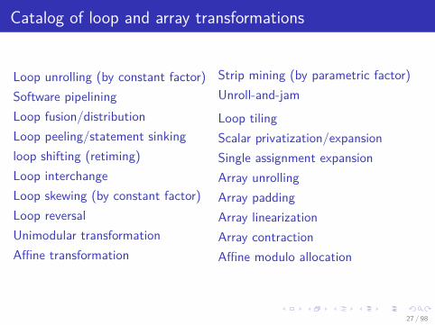
Catalog of loop and array transformations
Loop unrolling (by constant factor)Software pipeliningLoop fusion/distributionLoop peeling/statement sinkingloop shifting (retiming)Loop interchangeLoop skewing (by constant factor)Loop reversalUnimodular transformationAffine transformation
Strip mining (by parametric factor)Unroll-and-jam
Loop tilingScalar privatization/expansionSingle assignment expansionArray unrollingArray paddingArray linearizationArray contractionAffine modulo allocation
27 / 98
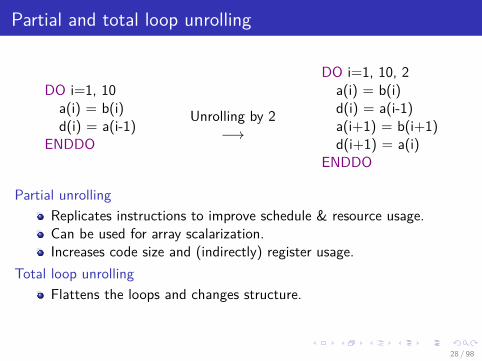
Partial and total loop unrolling
DO i=1, 10a(i) = b(i)d(i) = a(i-1)
ENDDO
Unrolling by 2−→
DO i=1, 10, 2a(i) = b(i)d(i) = a(i-1)a(i+1) = b(i+1)d(i+1) = a(i)
ENDDO
Partial unrollingReplicates instructions to improve schedule & resource usage.Can be used for array scalarization.Increases code size and (indirectly) register usage.
Total loop unrollingFlattens the loops and changes structure.
28 / 98

Strip mining, loop coalescing
DO i=1, Na(i) = b(i) + c(i)
ENDDO
Strip mining−→←−
Loop linearization
DO Is=1, N, sDO i=Is , min(N, Is+s-1)
a(i) = b(i) + c(i)ENDDO
ENDDO
Strip miningPerforms parametric loop unrolling.Changes the structure (2D space).Creates blocks of computations.Can be used as a preliminary step for tiling.
Loop linearizationCan reduce the control of loops.Reduces the problem dimension.
29 / 98

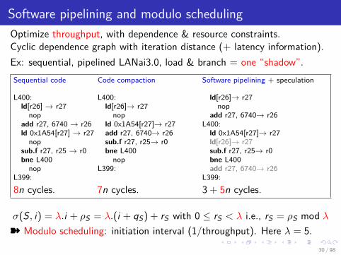
Software pipelining and modulo schedulingOptimize throughput, with dependence & resource constraints.Cyclic dependence graph with iteration distance (+ latency information).Ex: sequential, pipelined LANai3.0, load & branch = one “shadow”.Sequential code
L400:ld[r26] → r27nop
add r27, 6740 → r26ld 0x1A54[r27] → r27nop
sub.f r27, r25 → r0bne L400nop
L399:
8n cycles.
C
D
B
A
E
1,10,2
0,2
0,−1
0,2
0,1 1,1
1,−1
σ(S, i) = λ.i + ρS = λ.(i + qS) + rS with 0 ≤ rS < λ i.e., rS = ρS mod λý Modulo scheduling: initiation interval (1/throughput). Here λ = 5.
30 / 98

Software pipelining and modulo schedulingOptimize throughput, with dependence & resource constraints.Cyclic dependence graph with iteration distance (+ latency information).Ex: sequential, pipelined LANai3.0, load & branch = one “shadow”.Sequential code
L400:ld[r26] → r27nop
add r27, 6740 → r26ld 0x1A54[r27] → r27nop
sub.f r27, r25 → r0bne L400nop
L399:
8n cycles.
Code compaction
L400:ld[r26]→ r27nop
add r27, 6740→ r26ld 0x1A54[r27]→ r27nop
sub.f r27, r25→ r0bne L400nop
L399:
C
D
B
A
E
1,10,2
0,2
0,−1
0,2
0,1 1,1
1,−1
σ(S, i) = λ.i + ρS = λ.(i + qS) + rS with 0 ≤ rS < λ i.e., rS = ρS mod λý Modulo scheduling: initiation interval (1/throughput). Here λ = 5.
30 / 98

Software pipelining and modulo schedulingOptimize throughput, with dependence & resource constraints.Cyclic dependence graph with iteration distance (+ latency information).Ex: sequential, pipelined LANai3.0, load & branch = one “shadow”.Sequential code
L400:ld[r26] → r27nop
add r27, 6740 → r26ld 0x1A54[r27] → r27nop
sub.f r27, r25 → r0bne L400nop
L399:
8n cycles.
Code compaction
L400:ld[r26]→ r27nop
ld 0x1A54[r27]→ r27add r27, 6740→ r26nop
sub.f r27, r25→ r0bne L400nop
L399:
C
D
B
A
E
1,10,2
0,2
0,−1
0,2
0,1 1,1
1,−1
σ(S, i) = λ.i + ρS = λ.(i + qS) + rS with 0 ≤ rS < λ i.e., rS = ρS mod λý Modulo scheduling: initiation interval (1/throughput). Here λ = 5.
30 / 98

Software pipelining and modulo schedulingOptimize throughput, with dependence & resource constraints.Cyclic dependence graph with iteration distance (+ latency information).Ex: sequential, pipelined LANai3.0, load & branch = one “shadow”.Sequential code
L400:ld[r26] → r27nop
add r27, 6740 → r26ld 0x1A54[r27] → r27nop
sub.f r27, r25 → r0bne L400nop
L399:
8n cycles.
Code compaction
L400:ld[r26]→ r27nop
ld 0x1A54[r27]→ r27add r27, 6740→ r26sub.f r27, r25→ r0bne L400nop
L399:
7n cycles.
C
D
B
A
E
1,10,2
0,2
0,−1
0,2
0,1 1,1
1,−1
σ(S, i) = λ.i + ρS = λ.(i + qS) + rS with 0 ≤ rS < λ i.e., rS = ρS mod λý Modulo scheduling: initiation interval (1/throughput). Here λ = 5.
30 / 98

Software pipelining and modulo schedulingOptimize throughput, with dependence & resource constraints.Cyclic dependence graph with iteration distance (+ latency information).Ex: sequential, pipelined LANai3.0, load & branch = one “shadow”.Sequential code
L400:ld[r26] → r27nop
add r27, 6740 → r26ld 0x1A54[r27] → r27nop
sub.f r27, r25 → r0bne L400nop
L399:
8n cycles.
C
D
B
A
E
1,10,2
0,2
0,−1
0,2
0,1 1,1
1,−1
Software pipelining
L400:ld[r26]→ r27nop
add r27, 6740→ r26ld 0x1A54[r27], r27nop
sub.f r27, r25→ r0bne L400nop
L399:
σ(S, i) = λ.i + ρS = λ.(i + qS) + rS with 0 ≤ rS < λ i.e., rS = ρS mod λý Modulo scheduling: initiation interval (1/throughput). Here λ = 5.
30 / 98

Software pipelining and modulo schedulingOptimize throughput, with dependence & resource constraints.Cyclic dependence graph with iteration distance (+ latency information).Ex: sequential, pipelined LANai3.0, load & branch = one “shadow”.Sequential code
L400:ld[r26] → r27nop
add r27, 6740 → r26ld 0x1A54[r27] → r27nop
sub.f r27, r25 → r0bne L400nop
L399:
8n cycles.
C
D
B
A
E
1,10,2
0,2
0,−1
0,2
0,1 1,1
1,−1
Software pipelining
ld[r26]→ r27nop
add r27, 6740→ r26L400:
ld 0x1A54[r27]→ r27nop
sub.f r27, r25→ r0bne L400nop
ld[r26]→ r27nop
add r27, 6740→ r26L399:
σ(S, i) = λ.i + ρS = λ.(i + qS) + rS with 0 ≤ rS < λ i.e., rS = ρS mod λý Modulo scheduling: initiation interval (1/throughput). Here λ = 5.
30 / 98

Software pipelining and modulo schedulingOptimize throughput, with dependence & resource constraints.Cyclic dependence graph with iteration distance (+ latency information).Ex: sequential, pipelined LANai3.0, load & branch = one “shadow”.Sequential code
L400:ld[r26] → r27nop
add r27, 6740 → r26ld 0x1A54[r27] → r27nop
sub.f r27, r25 → r0bne L400nop
L399:
8n cycles.
C
D
B
A
E
1,10,2
0,2
0,−1
0,2
0,1 1,1
1,−1
Software pipelining + speculation
ld[r26]→ r27nop
add r27, 6740→ r26L400:
ld 0x1A54[r27]→ r27ld[r26]→ r27sub.f r27, r25→ r0bne L400add r27, 6740→ r26
L399:
3 + 5n cycles.
σ(S, i) = λ.i + ρS = λ.(i + qS) + rS with 0 ≤ rS < λ i.e., rS = ρS mod λý Modulo scheduling: initiation interval (1/throughput). Here λ = 5.
30 / 98
Software pipelining and modulo schedulingOptimize throughput, with dependence & resource constraints.Cyclic dependence graph with iteration distance (+ latency information).Ex: sequential, pipelined LANai3.0, load & branch = one “shadow”.Sequential code
L400:ld[r26] → r27nop
add r27, 6740 → r26ld 0x1A54[r27] → r27nop
sub.f r27, r25 → r0bne L400nop
L399:
8n cycles.
Code compaction
L400:ld[r26]→ r27nop
ld 0x1A54[r27]→ r27add r27, 6740→ r26sub.f r27, r25→ r0bne L400nop
L399:
7n cycles.
Software pipelining + speculation
ld[r26]→ r27nop
add r27, 6740→ r26L400:
ld 0x1A54[r27]→ r27ld[r26]→ r27sub.f r27, r25→ r0bne L400add r27, 6740→ r26
L399:
3 + 5n cycles.
σ(S, i) = λ.i + ρS = λ.(i + qS) + rS with 0 ≤ rS < λ i.e., rS = ρS mod λý Modulo scheduling: initiation interval (1/throughput). Here λ = 5.
30 / 98

Loop shifting or retiming
DO i=1, Na(i) = b(i)d(i) = a(i-1)
ENDDO
Loop shifting←→
DO i=0, NIF (i > 0) THEN
a(i) = b(i)IF (i < N) THEN
d(i+1) = a(i)ENDDO
Here: dependence at distance 1 (loop-carried or inter-iteration) transformedinto dependence at distance 0 (loop-independent or intra-iteration).
Main featuresSimilar to software pipelining.Creates prelude/postlude or introduces if statements.Can be used to align accesses and enable loop fusion.Particularly suitable to handle constant dependence distances.
31 / 98

Loop peeling and statement sinking
DO i=0, NIF (i > 0) THENa(i) = b(i)
IF (i < N) THENd(i+1) = a(i)
ENDDO
Loop peeling−→←−
Statement sinking
d(1) = a(0)DO i=1, N-1a(i) = b(i)d(i+1) = a(i)
ENDDOa(N) = b(N)
Loop peelingRemoves a few iterations to make code simpler.May enable more transformations.Reduces the iteration domain (range of loop counter).
Statement sinkingUsed to make loops perfectly nested.
32 / 98

Loop distribution and loop fusion
DO i=1, Na(i) = b(i)d(i) = a(i-1)
ENDDO
Loop distribution−→←−
Loop fusion
DO i=1, Na(i) = b(i)
ENDDODO i=1, Nd(i) = a(i-1)
ENDDOHere: intra-loop dependence transformed into inter-loop dependence.
Loop distributionUsed to parallelize/vectorize loops (no inter-iteration dependence).Valid if statements not involved in a circuit of dependences.Parallelization: separate strongly connected components.
Loop fusionIncreases the granularity of computations.Reduces loop overhead.Usually improves spatial & temporal data locality.May enable array scalarization.
33 / 98

Loop parallelization with loop distribution
DO i=1,NA(i) = 2*A(i) + 1B(i) = C(i-1) + A(i)C(i) = C(i-1) + G(i)D(i) = D(i-1) + A(i) + C(i-1)E(i) = E(i-1) + B(i)F(i) = D(i) + B(i-1)
ENDDO
B
AC
D
E F
1
10
1
0
1
01
0
1
Instance of typed loop fusion, with 2 types (par. & seq.), and possiblyfusion-preventing edges for 1 type (par.). * NP-complete.
34 / 98

Loop parallelization with loop distributionDOPAR i=1,N
A(i) = 2*A(i) + 1ENDDOPARDOSEQ i=1,NC(i) = C(i-1) + G(i)
ENDDOSEQDOPAR i=1,NB(i) = C(i-1) + A(i)
ENDDOPARDOSEQ i=1,NE(i) = E(i-1) + B(i)
ENDDOSEQDOSEQ i=1,ND(i) = D(i-1) + A(i) + C(i-1)
ENDDOSEQDOPAR i=1,NF(i) = D(i) + B(i-1)
ENDDOPAR
B
AC
D
E F
1
10
1
0
1
01
0
1
Instance of typed loop fusion, with 2 types (par. & seq.), and possiblyfusion-preventing edges for 1 type (par.). * NP-complete.
34 / 98

Loop parallelization with partial loop distribution
DOSEQ i=1,NC(i) = C(i-1) + G(i)
ENDDOSEQDOPAR i=1,NA(i) = 2*A(i) + 1B(i) = C(i-1) + A(i)
ENDDOPARDOSEQ i=1,ND(i) = D(i-1) + A(i) + C(i-1)E(i) = E(i-1) + B(i)
ENDDOSEQDOPAR i=1,NF(i) = D(i) + B(i-1)
ENDDOPAR
B
AC
D
E F
1
10
1
0
1
01
0
1
Instance of typed loop fusion, with 2 types (par. & seq.), and possiblyfusion-preventing edges for 1 type (par.). * NP-complete.
34 / 98

Loop shifting and loop parallelization
Maximal typed fusion Easy for 1 type, NP-complete for ≥ 2 types.
DO i=2, na(i) = f(i)b(i) = g(i)c(i) = a(i-1) + b(i)d(i) = a(i) + b(i-1)e(i) = d(i-1) + d(i)
ENDDO
simple precedence
prevents fusion
C D
B
E
ADOPAR i=2, na(i) = f(i)b(i) = g(i)
ENDDOPARDOPAR i=2, nc(i) = a(i-1) + b(i)d(i) = a(i) + b(i-1)
ENDDOPARDOPAR i=2, ne(i) = d(i-1) + d(i)
ENDDO
Same problem with loop shifting?
DO i=2, na(i) = f(i)b(i) = g(i)c(i) = a(i-1) + b(i)d(i) = a(i) + b(i-1)e(i) = d(i-1) + d(i)
ENDDO C D
A B
E
11
0 1
00
DOPAR i=2, na(i) = f(i)b(i) = g(i)
ENDDOPARDOPAR i=2, nc(i) = a(i-1) + b(i)d(i) = a(i) + b(i-1)
ENDDOPARDOPAR i=2, ne(i) = d(i-1) + d(i)
ENDDO
35 / 98

Loop shifting and loop parallelization
Maximal typed fusion Easy for 1 type, NP-complete for ≥ 2 types.
DO i=2, na(i) = f(i)b(i) = g(i)c(i) = a(i-1) + b(i)d(i) = a(i) + b(i-1)e(i) = d(i-1) + d(i)
ENDDO
simple precedence
prevents fusion
C D
B
E
ADOPAR i=2, na(i) = f(i)b(i) = g(i)
ENDDOPARDOPAR i=2, nc(i) = a(i-1) + b(i)d(i) = a(i) + b(i-1)
ENDDOPARDOPAR i=2, ne(i) = d(i-1) + d(i)
ENDDO
Same problem with loop shifting? NP-complete even for 1 type.
DO i=2, na(i) = f(i)b(i) = g(i)c(i) = a(i-1) + b(i)d(i) = a(i) + b(i-1)e(i) = d(i-1) + d(i)
ENDDO C D
A B
E
01
0 1
0
+1−1
a(2) = f(2)d(2) = a(2) + b(1)DOPAR i=3, na(i) = f(i)b(i-1) = g(i-1)d(i) = a(i) + b(i-1)
ENDDOPARb(n) = g(n)DOPAR i=2, nc(i) = a(i-1) + b(i)e(i) = d(i-1) + d(i)
ENDDOPAR
35 / 98

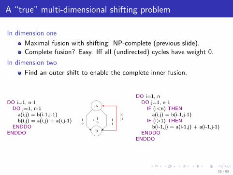
A “true” multi-dimensional shifting problem
In dimension oneMaximal fusion with shifting: NP-complete (previous slide).Complete fusion? Easy. Iff all (undirected) cycles have weight 0.
In dimension twoFind an outer shift to enable the complete inner fusion.
NP-complete (as many other retiming problems).
DO i=1, n-1DO j=1, n-1a(i,j) = b(i-1,j-1)b(i,j) = a(i,j) + a(i,j-1)
ENDDOENDDO
A
B
00
01
11
DO i=1, n-1DOPAR j=1, n-1a(i,j) = b(i-1,j-1)
ENDDOPARDOPAR j=1, n-1b(i,j) = a(i,j) + a(i,j-1)
ENDDOPARENDDO
* These are very particular problems & instances, but still, this shows thedifficulty to “push” dependences inside, i.e., to optimize locality.
36 / 98
A “true” multi-dimensional shifting problem
In dimension oneMaximal fusion with shifting: NP-complete (previous slide).Complete fusion? Easy. Iff all (undirected) cycles have weight 0.
In dimension twoFind an outer shift to enable the complete inner fusion.
NP-complete (as many other retiming problems).
DO i=1, n-1DO j=1, n-1a(i,j) = b(i-1,j-1)b(i,j) = a(i,j) + a(i,j-1)
ENDDOENDDO
+
A
B
10
11
10
10
DO i=1, nDO j=1, n-1IF (i<n) THENa(i,j) = b(i-1,j-1)
IF (i>1) THENb(i-1,j) = a(i-1,j) + a(i-1,j-1)
ENDDOENDDO
* These are very particular problems & instances, but still, this shows thedifficulty to “push” dependences inside, i.e., to optimize locality.
36 / 98

A “true” multi-dimensional shifting problem
In dimension oneMaximal fusion with shifting: NP-complete (previous slide).Complete fusion? Easy. Iff all (undirected) cycles have weight 0.
In dimension twoFind an outer shift to enable the complete inner fusion.NP-complete (as many other retiming problems).
DO i=1, n-1DO j=1, n-1a(i,j) = b(i-1,j-1)b(i,j) = a(i,j) + a(i,j-1)
ENDDOENDDO
+
A
B
11
12
00
11
DO i=1, nDOPAR j=1, nIF (i>1) and (j>1) THENb(i-1,j-1) = a(i-1,j-1) + a(i-1,j-2)
IF (i<n) and (j<n) THENa(i,j) = b(i-1,j-1)
ENDDOPARENDDO
* These are very particular problems & instances, but still, this shows thedifficulty to “push” dependences inside, i.e., to optimize locality.
36 / 98

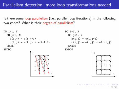
Parallelism detection: more loop transformations needed
Is there some loop parallelism (i.e., parallel loop iterations) in the followingtwo codes? What is their degree of parallelism?
DO i=1, NDO j=1, N
a(i,j) = c(i,j-1)c(i,j) = a(i,j) + a(i-1,N)
ENDDOENDDO
i
j
DO i=1, NDO j=1, N
a(i,j) = c(i,j-1)c(i,j) = a(i,j) + a(i-1,j)
ENDDOENDDO
i
j
37 / 98

Loop interchange
Loop interchange: (i , j) 7→ (j , i).
DO i=1, NDO j=1, ia(i,j+1) = a(i,j) + 1
ENDDOENDDO
Loop interchange←→
DO j=1, NDO i=j, N
a(i,j+1) = a(i,j) + 1ENDDO
ENDDO
Here: dependence distance (0, 1) transformed into distance (1, 0).
Main featuresMay involve bounds computations as in
n∑i=1
i∑j=1
Si ,j =n∑
j=1
n∑i=j
Si ,j .Can impact loop parallelism.Basis of loop tiling.Changes order of memory accesses and thus data locality.
38 / 98

Unroll-and-jam
DO i=1, 2NDO j=1, Ma(i,j) = . . .
ENDDOENDDO
Unroll-and-jam←→
DO i=0, 2N, 2DO j=0, Ma(i,j) = . . .a(i+1,j) = . . .
ENDDOENDDO
Interests:Combines outer loop unrolling and loop fusion.Changes order of iterations and locality, keeping same loop nesting.Can be viewed as a restricted form of tiling s × 1.
39 / 98
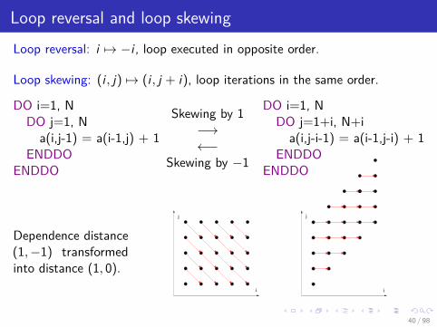
Loop reversal and loop skewingLoop reversal: i 7→ −i , loop executed in opposite order.
Loop skewing: (i , j) 7→ (i , j + i), loop iterations in the same order.
DO i=1, NDO j=1, Na(i,j-1) = a(i-1,j) + 1
ENDDOENDDO
Skewing by 1−→←−
Skewing by −1
DO i=1, NDO j=1+i, N+ia(i,j-i-1) = a(i-1,j-i) + 1
ENDDOENDDO
Dependence distance(1,−1) transformedinto distance (1, 0).
i
j
i
j
40 / 98

Unimodular transf.: reversal + skewing + interchangeDO i=1, N
DO j=1, Na(i,j) = . . .
ENDDOENDDO
Unimodular U−→←−
Unimodular U−1
DO t=2, 2NDO p=max(1,t-N), min(N,t-1)a(p,t-p) = . . .
ENDDOENDDO
Here, (i , j) 7→ (t, p) = (i + j , i). Loop bounds with Fourier-Motzkin elim.:
1 ≤ i , j ≤ N ⇔ 1 ≤ p, t − p ≤ N ⇔ 1 ≤ p ≤ N, t − N ≤ p ≤ t − 1Elimination of p ⇒ 2 ≤ t ≤ 2N, 1 ≤ N, Elimination of t ⇒ 1 ≤ N
In general: “For all ~i ∈ P do S(~i)” −→ “For all ~p ∈ UP do S(U−1~p)”.(tp
)= U
(ij
) (ij
)= U−1
(tp
)Here U =
(1 11 0
)U−1 =
(0 11 −1
)New implicit execution order: iterate lexicographically on (t, p).If S(~i) depends on T (~j), dep. distance d =~i −~j lexico-positive: ~d lex ~0.New distance ~d ′ = U(~i −~j) = U~d . Validity condition: ~d ′ = U~d lex ~0.
41 / 98

Loop tiling, blocked algorithms
DO t=2, 2NDOPAR j=max(1,t-N), min(N,t-1)
a(t-j,j) = c(t-j,j-1)c(t-j,j) = a(t-j,j) + a(t-j-1,j)
ENDDOENDDO i
j
DO I=1, N, BDO J=1, N, B
DO i=I, min(I+B-1,N)DO j=J, min(J+B-1,N)
a(i,j) = c(i,j-1)c(i,j) = a(i,j) + a(i-1,j)
ENDDOENDDO
ENDDOENDDO
i
j
ý Tiling and parallelism detection: similar problem.
42 / 98

In practice, need to combine all. Ex: HLS with C2H AlteraOptimize DDR accesses for bandwidth-bound accelerators.
Use tiling for data reuse and to enable burst communication.Use fine-grain software pipelining to pipeline DDR requests.Use double buffering to hide DDR latencies.Use coarse-grain software pipelining to hide computations.
iterations
time
=STORE0
STORE1
STORE0
STORE1
Note:
dependence synchro.
DDR access synchro.
COMP1
COMP0
COMP1
COMP0
Load(T) at time 2T
Comp(T) at time 2T+2
Store(T) at time 2T+5
LOAD0
LOAD1
LOAD0
LOAD1
43 / 98

SYSTEMS OF UNIFORMRECURRENCE EQUATIONS
44 / 98

SURE: system of uniform recurrence equations (1967)
Karp, Miller, Winograd: “The organization of computations for uniformrecurrence equations” (J. ACM, 14(3), pp. 563-590).
∀~p ∈ ~p = (i , j) | 1 ≤ i , j ≤ N a(i , j) = c(i , j − 1)b(i , j) = a(i − 1, j) + b(i , j + 1)c(i , j) = a(i , j) + b(i , j)
00
a
b
c
10
0-1
00
01
RDG (reduced dependence graph) G = (V ,E , ~w).EDG (expanded dep. graph): vertices V × P = unrolled RDG.
Semantics:Explicit dependences, implicit schedule.Compute left-hand side first, unless not in P (input data).
45 / 98
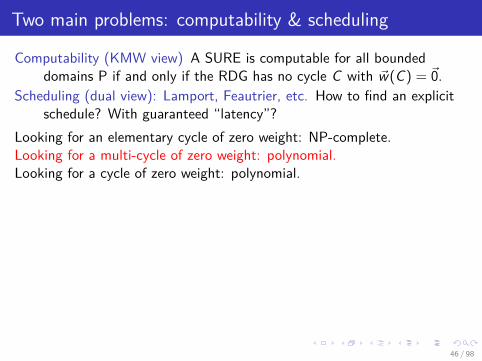
Two main problems: computability & scheduling
Computability (KMW view) A SURE is computable for all boundeddomains P if and only if the RDG has no cycle C with ~w(C) = ~0.
Scheduling (dual view): Lamport, Feautrier, etc. How to find an explicitschedule? With guaranteed “latency”?
Looking for an elementary cycle of zero weight: NP-complete.Looking for a multi-cycle of zero weight: polynomial.Looking for a cycle of zero weight: polynomial.
Key structure: the subgraph G ′ induced by all edges that belong to amulti-cycle (i.e., union of cycles) of zero weight.
G :
00
a
b
c
10
0-1
00
01
G and G ′:
00
a
b
c
10
0-1
00
01
46 / 98

Two main problems: computability & scheduling
Computability (KMW view) A SURE is computable for all boundeddomains P if and only if the RDG has no cycle C with ~w(C) = ~0.
Scheduling (dual view): Lamport, Feautrier, etc. How to find an explicitschedule? With guaranteed “latency”?
Looking for an elementary cycle of zero weight: NP-complete.Looking for a multi-cycle of zero weight: polynomial.Looking for a cycle of zero weight: polynomial.Key structure: the subgraph G ′ induced by all edges that belong to amulti-cycle (i.e., union of cycles) of zero weight.
G :
00
a
b
c
10
0-1
00
01
G and G ′:
00
a
b
c
10
0-1
00
01
46 / 98
Key properties for multi-dimensional decomposition
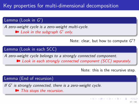
Lemma (Look in G ′)A zero-weight cycle is a zero-weight multi-cycle.
ý Look in the subgraph G ′ only.
Note: clear, but how to compute G ′?
Lemma (Look in each SCC)A zero-weight cycle belongs to a strongly connected component.
ý Look in each strongly connected component (SCC) separately.
Note: this is the recursive step.
Lemma (End of recursion)If G ′ is strongly connected, there is a zero-weight cycle.
ý This stops the recursion.
47 / 98

Key properties for multi-dimensional decomposition
Lemma (End of recursion)If G ′ is strongly connected, there is a zero-weight cycle.
e1 e2
e3e4
P1 P2
P3P4
C1’
C3’
C3’
∑i ei cycle that visits
all vertices.ei in multi-cycle Ci ,with ~w(Ci ) = ~0.Ci = ei + Pi + C ′i .Follow the ei , then thePi and, on the way,plug the C ′i .
48 / 98

Karp, Miller, and Winograd’s decompositionBoolean KMW(G):
Build G ′ the subgraph of zero-weight multicycles of G .Compute G ′1, . . . , G ′s , the s SCCs of G ′.
If s = 0, G ′ is empty, return TRUE.If s = 1, G ′ is strongly connected, return FALSE.Otherwise return ∧iKMW(G ′
i ) (logical AND).Then, G is computable iff KMW(G) returns TRUE.
Depth d = 0 if G acyclic, d = 1 if all SCCs have an empty G ′, etc.
Theorem (Depth of the decomposition)If G is computable, d ≤ n (dimension of P). Otherwise, d ≤ n + 1.
Theorem (Optimal number of parallel loops)If Ω(N)2 ⊆ P ⊆ O(N)2, there is a dependence path of length Ω(Nd ) andone can build an affine schedule of latency O(Nd ) * “optimal”
49 / 98

But how to compute G ′? Primal and dual programs.
e ∈ G ′ iff ve = 0 in any optimal solution of the linear program:
min ∑
e ve | ~q ≥ ~0, ~v ≥ ~0, ~q + ~v ≥ ~1, C~q = ~0, W~q = ~0
Always interesting to take a look at the dual program:
max ∑
e ze | ~0 ≤ ~z ≤ ~1, ~X .~w(e) + ρv − ρu ≥ ze , ∀e = (u, v) ∈ E
* Generalizes modulo scheduling: σ(u, ~p) = ~X .~p + ρu (in 1D: λ.p + ρu).
For any optimal solution:e /∈ G ′ ⇔ ~X .~w(e) + ρv − ρu ≥ 1
* loop carried
.e ∈ G ′ ⇔ ~X .~w(e) + ρv − ρu = 0
* loop independent
.and keep going until all dependences become carried.
* Multi-dimensional scheduling and loop transformations.
50 / 98

But how to compute G ′? Primal and dual programs.
e ∈ G ′ iff ve = 0 in any optimal solution of the linear program:
min ∑
e ve | ~q ≥ ~0, ~v ≥ ~0, ~q + ~v ≥ ~1, C~q = ~0, W~q = ~0
Always interesting to take a look at the dual program:
max ∑
e ze | ~0 ≤ ~z ≤ ~1, ~X .~w(e) + ρv − ρu ≥ ze , ∀e = (u, v) ∈ E
* Generalizes modulo scheduling: σ(u, ~p) = ~X .~p + ρu (in 1D: λ.p + ρu).
For any optimal solution:e /∈ G ′ ⇔ ~X .~w(e) + ρv − ρu ≥ 1 * loop carried.e ∈ G ′ ⇔ ~X .~w(e) + ρv − ρu = 0 * loop independent.
and keep going until all dependences become carried.
* Multi-dimensional scheduling and loop transformations.
50 / 98

Scheduling/parallelization of illustrating example
00
a
b
c
10
0-1
00
01
~X1.(0, 1) = 0~X1.(1, 0) ≥ 2
⇒
~X1 = (2, 0), ρa = 1ρb = 0, ρc = 1
Final schedule
σa(i , j) = (2i + 1, 2j)σb(i , j) = (2i ,−j)σc(i , j) = (2i + 1, 2j + 1)
∀~p ∈ ~p = (i , j) | 1 ≤ i , j ≤ N a(i , j) = c(i , j − 1)b(i , j) = a(i − 1, j) + b(i , j + 1)c(i , j) = a(i , j) + b(i , j)
DO i=1, NDO j=N, 1, -1b(i,j) = a(i-1,j) + b(i,j+1)
ENDDODO j=1, Na(i,j) = c(i,j-1)c(i,j) = a(i,j) + b(i,j)
ENDDOENDDO
* Today: most work based on Farkas lemma (affine form) followingFeautrier (1992) & generalized tiling as Pluto (2008).
51 / 98

DETECTION OF LOOPPARALLELISM
52 / 98

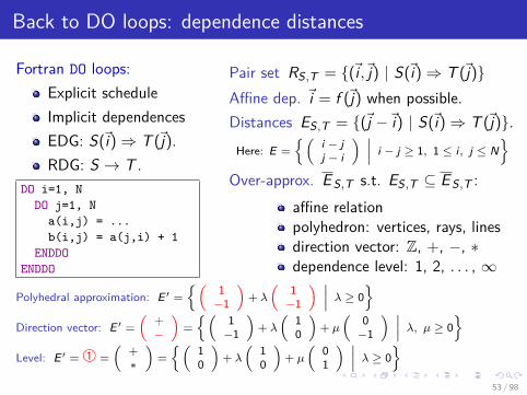
Back to DO loops: dependence distances
Fortran DO loops:Explicit scheduleImplicit dependencesEDG: S(~i)⇒ T (~j).RDG: S → T .
DO i=1, NDO j=1, N
a(i,j) = ...b(i,j) = a(j,i) + 1
ENDDOENDDO
Pair set RS,T = (~i ,~j) | S(~i)⇒ T (~j)Affine dep. ~i = f (~j) when possible.Distances ES,T = (~j −~i) | S(~i)⇒ T (~j).
Here: E =
(i − jj − i
) ∣∣∣ i − j ≥ 1, 1 ≤ i , j ≤ N
Over-approx. ES,T s.t. ES,T ⊆ ES,T :affine relationpolyhedron: vertices, rays, linesdirection vector: Z, +, −, ∗dependence level: 1, 2, . . . , ∞
Polyhedral approximation: E ′ =(
1−1
)+ λ
(1−1
) ∣∣∣ λ ≥ 0
Direction vector: E ′ =(
+−
)=
(1−1
)+ λ
(10
)+ µ
(0−1
) ∣∣∣ λ, µ ≥ 0
Level: E ′ = À =
(+∗
)=
(10
)+ λ
(10
)+ µ
(01
) ∣∣∣ λ ≥ 0
53 / 98
Back to DO loops: dependence distances
Fortran DO loops:Explicit scheduleImplicit dependencesEDG: S(~i)⇒ T (~j).RDG: S → T .
DO i=1, NDO j=1, N
a(i,j) = ...b(i,j) = a(j,i) + 1
ENDDOENDDO
Pair set RS,T = (~i ,~j) | S(~i)⇒ T (~j)Affine dep. ~i = f (~j) when possible.Distances ES,T = (~j −~i) | S(~i)⇒ T (~j).Here: E =
(i − jj − i
) ∣∣∣ i − j ≥ 1, 1 ≤ i , j ≤ N
Over-approx. ES,T s.t. ES,T ⊆ ES,T :affine relationpolyhedron: vertices, rays, linesdirection vector: Z, +, −, ∗dependence level: 1, 2, . . . , ∞
Polyhedral approximation: E ′ =(
1−1
)+ λ
(1−1
) ∣∣∣ λ ≥ 0
Direction vector: E ′ =(
+−
)=
(1−1
)+ λ
(10
)+ µ
(0−1
) ∣∣∣ λ, µ ≥ 0
Level: E ′ = À =
(+∗
)=
(10
)+ λ
(10
)+ µ
(01
) ∣∣∣ λ ≥ 0
53 / 98

Uniformization of dependences: example
DO i=1, NDO j=1, N
S: a(i,j) = c(i,j-1)T: c(i,j) = a(i,j) + a(i-1,N)
ENDDOENDDO
S(i-1,N) ⇒ T(i,j)Dep. distance (1, j − N).
Direction vector (1, 0−) = (1, 0) + k(0,−1), k ≥ 0 * SURE! KMW!
S
00
01
10-
T
00
S
S’10
0-1
00
01
T
No parallelism (d = 2). Code appears purely sequential (and here it is).
54 / 98
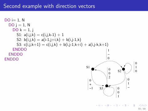
Second example with direction vectors
DO i= 1, NDO j = 1, NDO k = 1, j
S1: a(i,j,k) = c(i,j,k-1) + 1S2: b(i,j,k) = a(i-1,j+i,k) + b(i,j-1,k)S3: c(i,j,k+1) = c(i,j,k) + b(i,j-1,k+i) + a(i,j-k,k+1)
ENDDOENDDO
ENDDO
1
−
0
0
1
−
0
+
−1
0
0
2
0
1
0
0
0
1
S1
S3
S2
55 / 98

Second example: dependence graphs
1
−
0
0
1
−
0
+
−1
0
0
2
0
1
0
0
0
1
S1
S3
S2
Initial RDG.
0
0
2
0
1
00
1
−1
0
0
0
0
−1
0 0
0
0
0
0
0
1
−1
0
0
1
0
0
1
−1
0
0
1
0
0
−1
S1
S3
S2
Uniformized RDG.
56 / 98

Second example: G and G ′
0
0
2
0
1
00
1
−1
0
0
0
0
−1
0 0
0
0
0
0
0
1
−1
0
0
1
0
0
1
−1
0
0
1
0
0
−1
S1
S3
S2
Uniformized RDG.
0
0
2
0
1
00
1
−1
0
0
0
0
−1
0
0
1
00
0
1
0
0
−1
S1
S3
S2
G ′: zero-weight multi-cycles.
(2i , j) for S2, (2i + 1, 2k) for S1, and (2i + 1, 2k + 3) for S3.
57 / 98

Second exemple: parallel code generationDOSEQ i=1, n
DOSEQ j=1, n /* scheduling (2i, j) for S2*/DOPAR k=1, jS2: b(i,j,k) = a(i-1,j+i,k) + b(i,j-1,k)
ENDDOPARENDDOSEQDOSEQ k = 1, n+1IF (k ≤ n) THEN /* scheduling (2i+1, 2k) for S1*/DOPAR j=k, nS1: a(i,j,k) = c(i,j,k-1) + 1
ENDDOPARIF (k ≥ 2) THEN /* scheduling (2i+1, 2k+3) for S3*/DOPAR j=k-1, nS3: c(i,j,k) = c(i,j,k-1) + b(i,j-1,k+i-1) + a(i,j-k+1,k)
ENDDOPARENDDOSEQ
ENDDOSEQ ã Loop distribution of j , k loops: S2 then S1 + S3.ã Loop interchange of j and k loops for S1 and S3.ã Loop shifting in k, then loop distribution of j loop.
58 / 98

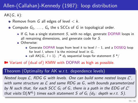
Allen-(Callahan)-Kennedy (1987): loop distributionAK(G , k):
Remove from G all edges of level < k.Compute G1, . . . , Gs the s SCCs of G in topological order.
If Gi has a single statement S, with no edge, generate DOPAR loops inall remaining dimensions, and generate code for S.Otherwise:
Generate DOPAR loops from level k to level l − 1, and a DOSEQ loopfor level l , where l is the minimal level in Gi .call AK(Gi , l + 1). /* dS sequential loops for statement S */
ý Variant of (dual of) KMW with DOPAR as high as possible.
Theorem (Optimality for AK w.r.t. dependence levels)Nested loops L, RDG G with levels. One can build some nested loops L′,with same structure as L and same RDG as G, with bounds parameterizedby N such that, for each SCC Gi of G, there is a path in the EDG of L′that visits Ω(Nds ) times each statement S of Gi (dS : depth w.r.t. S).
59 / 98

Darte-Vivien (1997): unimodular + shift + distribution
Boolean DV(G , k) /* G uniformized graph, with virtual and actual nodes */Build G ′ generated by the zero-weight multi-cycles of G .Modify slightly G ′ (technical detail not explained here).Choose ~X (vector) and, for each S in G ′, ρS (scalar) s.t.:
if e = (u, v) ∈ G ′ or u is virtual, ~X .~w(e) + ρv − ρu ≥ 0if e /∈ G ′ and u is actual, ~X .~w(e) + ρv − ρu ≥ 1
For each actual node S of G let ρkS = ρS and ~X k
S = ~X .Compute G ′1, . . . , G ′s the SCC of G ′ with ≥ 1 actual node:
If G ′ is empty or has only virtual nodes, return true.If G ′ is strongly connected with ≥ 1 actual node, return false.
Otherwise, returns∧
i=1DV(G ′
i , k + 1) (∧
= logical and).
ý Dual of KMW after dependence uniformization. Analyzing the cycleweights in G ′ leads to a variant to get a max. number of permutable loops.
60 / 98

General affine multi-dimensional schedules (Feautrier)
Affine dependences (or even relations): T (~j) depends on S(~i) if (~i ,~j) ∈ Dewhere e = (S,T ) and De is a polyhedron.
Look for affine schedule σ such that σ(S,~i) <lex σ(T ,~j) for all(~i ,~j) ∈ De . Use affine form of Farkas lemma (mechanical operation).Write σ(S,~i) + εe ≤ σ(T ,~j) with ~ε ≥ ~0 and maximize the number ofdependence edges e such that εe ≥ 1.Remove edges e such that εe ≥ 1 and continue to get remainingdimensions * multi-dimensional affine schedule.
ý Generalization of the constraints used in the dual of KMW.
To perform tiling, look for several dimensions (permutable loops) such thatσ(T ,~j)− σ(S,~i) ≥ 0 instead of σ(T ,~j)− σ(S,~i) ≥ 1. But morecomplicated to avoid the ~0 solution and guarantee linear independence.Key idea in Pluto: minimize dependence distance σ(T ,~j)− σ(S,~i).
61 / 98
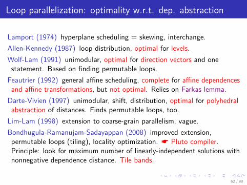
Loop parallelization: optimality w.r.t. dep. abstraction
Lamport (1974) hyperplane scheduling = skewing, interchange.Allen-Kennedy (1987) loop distribution, optimal for levels.Wolf-Lam (1991) unimodular, optimal for direction vectors and onestatement. Based on finding permutable loops.
Feautrier (1992) general affine scheduling, complete for affine dependencesand affine transformations, but not optimal. Relies on Farkas lemma.
Darte-Vivien (1997) unimodular, shift, distribution, optimal for polyhedralabstraction of distances. Finds permutable loops, too.
Lim-Lam (1998) extension to coarse-grain parallelism, vague.Bondhugula-Ramanujam-Sadayappan (2008) improved extension,permutable loops (tiling), locality optimization. * Pluto compiler.Principle: look for maximum number of linearly-independent solutions withnonnegative dependence distance. Tile bands.
62 / 98

Yet another application of SUREs: understand “iterations”
Fortran DO loops:DO i=1, N
DO j=1, Na(i,j) = c(i,j-1)c(i,j) = a(i,j) + a(i-1,N)
ENDDOENDDO
C for and while loops:y = 0; x = 0;while (x <= N && y <= N)
if (?) x=x+1;if (y >= 0 && ?) y=y-1;
y=y+1;
Uniform recurrence equations:∀p ∈ p = (i , j) | 1 ≤ i , j ≤ N a(i , j) = c(i , j − 1)
b(i , j) = a(i − 1, j) + b(i , j + 1)c(i , j) = a(i , j) + b(i , j)
00
a
b
c
10
0-1
00
01
63 / 98

KERNEL OFFLOADING ANDLOOP TILING
64 / 98

High-level synthesis (HLS) tools for FPGA
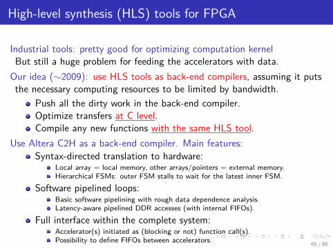
Industrial tools: pretty good for optimizing computation kernelBut still a huge problem for feeding the accelerators with data.
Our idea (∼2009): use HLS tools as back-end compilers, assuming it putsthe necessary computing resources to be limited by bandwidth.
Push all the dirty work in the back-end compiler.Optimize transfers at C level.Compile any new functions with the same HLS tool.
Use Altera C2H as a back-end compiler. Main features:Syntax-directed translation to hardware:
Local array = local memory, other arrays/pointers = external memory.Hierarchical FSMs: outer FSM stalls to wait for the latest inner FSM.
Software pipelined loops:Basic software pipelining with rough data dependence analysis.Latency-aware pipelined DDR accesses (with internal FIFOs).
Full interface within the complete system:Accelerator(s) initiated as (blocking or not) function call(s).Possibility to define FIFOs between accelerators.
Similar studyPouchet et al.FPGA’13 forXilinx AutoESL
65 / 98
High-level synthesis (HLS) tools for FPGA
Industrial tools: pretty good for optimizing computation kernelBut still a huge problem for feeding the accelerators with data.
Our idea (∼2009): use HLS tools as back-end compilers, assuming it putsthe necessary computing resources to be limited by bandwidth.
Push all the dirty work in the back-end compiler.Optimize transfers at C level.Compile any new functions with the same HLS tool.
Use Altera C2H as a back-end compiler. Main features:Syntax-directed translation to hardware:
Local array = local memory, other arrays/pointers = external memory.Hierarchical FSMs: outer FSM stalls to wait for the latest inner FSM.
Software pipelined loops:Basic software pipelining with rough data dependence analysis.Latency-aware pipelined DDR accesses (with internal FIFOs).
Full interface within the complete system:Accelerator(s) initiated as (blocking or not) function call(s).Possibility to define FIFOs between accelerators.
Similar studyPouchet et al.FPGA’13 forXilinx AutoESL
65 / 98

Throughput when accessing (asymmetric) DDR memoryEx: DDR-400 128Mbx8, size 16MB, CAS 3, 200MHz. Successive reads, same row= 10 ns , different rows = 80 ns . Even if fully pipelined (λ=1), a badspatial DDR locality can kill performances by a factor 8! Example:void vector_sum (int* __restrict__ a, b, c, int n)
for (int i = 0; i < n; i++) c[i] = a[i] + b[i];
/RAS
/CAS
/WE
DQ
PRECHARGE READ
ACTIVATE
load a(i)
a(i)
PRECHARGE READ
ACTIVATE
load b(i)
b(i)
store c(i)
PRECHARGE
ACTIVATE
WRITE
c(i)
C2H-compiled code: pipelined but time gaps & data thrown away.
0
1
2
3
4
5
6
7
2 4 8 16 32 64 128 256 512 1024 2048 4096 8192
Sp
ee
d-u
p
Block size
Typical figure withspeed-up vs block size(here vector sum).
66 / 98

Throughput when accessing (asymmetric) DDR memoryEx: DDR-400 128Mbx8, size 16MB, CAS 3, 200MHz. Successive reads, same row= 10 ns , different rows = 80 ns . Even if fully pipelined (λ=1), a badspatial DDR locality can kill performances by a factor 8! Example:void vector_sum (int* __restrict__ a, b, c, int n)
for (int i = 0; i < n; i++) c[i] = a[i] + b[i];
/RAS
/CAS
/WE
DQ
ACTIVATE
a(i) a(i+k)
PRECHARGE READ PRECHARGE READ
ACTIVATE
b(i) b(i+k)
store c(i) ... c(i+k)
PRECHARGE
ACTIVATE
WRITE
c(i) c(i+k)
load a(i) ... a(i+k) load b(i) ... b(i+k)
block size
Block version: reduces gaps, exploits bursts and temporal reuse.
0
1
2
3
4
5
6
7
2 4 8 16 32 64 128 256 512 1024 2048 4096 8192
Sp
ee
d-u
p
Block size
Typical figure withspeed-up vs block size(here vector sum).
66 / 98

Strip-mining and loop distribution?
Loop distribution: too large local memory.Unrolling: too many registers.
ý
strip-mining +loop distribution.
for (i=0; i<MAX; i=i+BLOCK) for(j=0; j<BLOCK; j++) a_tmp[j] = a[i+j]; //prefetchfor(j=0; j<BLOCK; j++) b_tmp[j] = b[i+j]; //prefetchfor(j=0; j<BLOCK; j++) c_tmp[i+j] = a_tmp[j] + b_tmp[j];for(j=0; j<BLOCK; j++) c[i+j] = c_tmp[i+j]; //store
ý Does not work!
first datareceived
latency
first request
DDR
i loop
time
pipeline
computation
j loop
fetch a,b
j loops
store
j loop
Accesses to arrays a and b stillinterleaved!Loop latency penalty.Outer loop not pipelined.
67 / 98

Introduce false dependences?
for (i=0; i<MAX; i=i+BLOCK) for(j=0; j<BLOCK; j++) tmp = BLOCK; a_tmp[j] = a[i+j];for(j=0; j<tmp; j++) b_tmp[j] = b[i+j];for(j=0; j<BLOCK; j++) c_tmp[i+j] = a_tmp[j] + b_tmp[j];for(j=0; j<BLOCK; j++) c[i+j] = c_tmp[i+j];
latency
first request
pipeline
j loop
fetch a
DDR
store
time
computation
j loop j loop
fetch b
first datareceived i loop
j loop
ý Still pay loop latency penalty and poor outermost loop pipeline.
68 / 98

Emulating (linearizing) nested loops?
i=0; j=0; bi=0;for (k=0; k<4*MAX; k++)
if (j==0) a_tmp[i] = a[bi+i];else if (j==1)
b_tmp[i] = b[bi+i];else if (j==2)
c_tmp[i] = a_tmp[i] + b_tmp[i];else c[bi+i] = c_tmp[i];
if (i<BLOCK-1) i++;else
i=0;if (j<3) j++;else j=0; bi = bi + BLOCK;
Need to use restrict pragmafor all arrays.λ = 21! Problem withdependence analyzer andsoftware pipeliner.Better behavior (λ = 3) withcase statement: by luck.Further loop unrolling to getλ = 1: too complex.But still a problem withinterleaved DDR accesses dueto speculative prefetching!
69 / 98

Emulating nested loops with a single transfer instruction?
i=0; j=0; bi=0;for (k=0; k<3*MAX; k++)
if (j==0) ptr_1 = &a[bi+i]; ptr_2 = &a_tmp[i]; else if (j==1) ptr_1 = &b[bi+i]; ptr_2 = &b_tmp[i]; else if (j==2) ptr_1 = &c_tmp[i]; ptr_2 = &c[bi+i];
c_tmp[i] = a_tmp[i] + b_tmp[i]; *ptr_2 = *ptr_1;
if (i<BLOCK-1) i++;else i=0; if (j<2) j++; else j=0; bi = bi + BLOCK;
No more interleaving between arrays a and b;λ not equal to 1, unless restrict pragma added: but leads to potentiallywrong codes (data dependences are lost).
How to decrease λ and generalize to more complex codes?* Communicating C processes, with suitable synchronizations.
70 / 98

Source-to-source transformations and kernel acceleration
How to optimize transfers automatically?
With C-level processes.
HLS tool FPGA boardVHDL codeC−code
General problem: porting applications on hardware acceleratorsEx: FPGA, GPU, dedicated board, multicore.Huge portability issue, costly compiler development.
Kernel offloading/function outliningHigh-productivity and high-performance languages.Library/directives-type support, e.g., OpenAcc.Source-to-source compilation, targeting back-end C dialects.
71 / 98

Source-to-source transformations and kernel acceleration
How to optimize transfers automatically? With C-level processes.
C−code
C−code
C−code
HLS toolOur tool FPGA boardVHDL codeC−code
General problem: porting applications on hardware acceleratorsEx: FPGA, GPU, dedicated board, multicore.Huge portability issue, costly compiler development.
Kernel offloading/function outliningHigh-productivity and high-performance languages.Library/directives-type support, e.g., OpenAcc.Source-to-source compilation, targeting back-end C dialects.
71 / 98

Source-to-source transformations and kernel acceleration
How to optimize transfers automatically? With C-level processes.
C−dialectcode
C−dialectcode
C−dialectcode
S2S tool AcceleratorC−code target codeSpecificBack−end
Compiler
General problem: porting applications on hardware acceleratorsEx: FPGA, GPU, dedicated board, multicore.Huge portability issue, costly compiler development.
Kernel offloading/function outliningHigh-productivity and high-performance languages.Library/directives-type support, e.g., OpenAcc.Source-to-source compilation, targeting back-end C dialects.
71 / 98

Data Movement between Memory Levels
Global Memory AcceleratorLocal Memoryslower faster
CPU Multi-level cache optimizationGPU Host to Global / Global to Shared / Shared to registersMPPA External DDR to multi scratch-padsFPGA External DDR to local memory
Computation by blocks * loop tilingTransfer optimization * intra-tile & inter-tile data reuseCommunication/computation overlap * pipeliningCost model * parametric tile sizes
72 / 98

Tiling, Data Reuse, and Pipelining
memory footprint
time remoteaccesses
tiling
tiling+ intra
tiling+ inter
tiling +pipeline
fullcopy
spatial locality
temporal locality
more reusefewer transfers
overlap
overlap
73 / 98

Tiling, Data Reuse, and Pipelining
memory footprint
time remoteaccesses
tiling
tiling+ intra
tiling+ inter
tiling +pipeline
fullcopy
spatial locality
temporal locality
more reusefewer transfers
overlap
overlap
73 / 98

Tiling, Data Reuse, and Pipelining
memory footprint
time remoteaccesses
tiling
tiling+ intra
tiling+ inter
tiling +pipeline
fullcopy
spatial locality
temporal locality
more reusefewer transfers
overlap
overlap
73 / 98
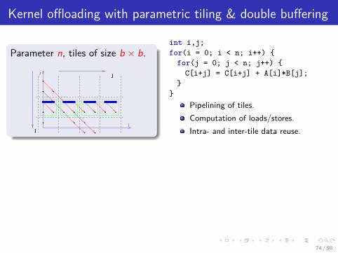
Kernel offloading with parametric tiling & double buffering
Parameter n, tiles of size b × b.
J
I
j
i
int i,j;for(i = 0; i < n; i++)
for(j = 0; j < n; j++) C[i+j] = C[i+j] + A[i]*B[j];
Pipelining of tiles.Computation of loads/stores.Intra- and inter-tile data reuse.
LoadC = m | 0 ≤ m, n − I − b ≤ m ≤ n − 1− I, J = 0∪ m | max(1, J) ≤ m + I − n + 1 ≤ min(n − 1, J + b − 1)
size 3b − 1 = (2b − 1) + b when n ≥ 2b + 1: 2 full tiles.size b + n − 1 = (2b − 1) + (n − b) when b ≤ n ≤ 2b: 1 full tile, 1 partial tile.size 2n − 1 when n ≤ b − 1: 1 partial tile.
* Parametric (not quadratic, but piece-wise affine), with possibleapproximations, corresponding liveness analysis, and memory mapping.
74 / 98

Loop tiling and permutable loops
j
i
A
BC
Product of two polynomials:arguments in A and B;result in C .dep. distance (1,−1).prevents permutation.
for (i=0, i<=2n-1; i++)c[i] = 0;
for (i=0; i<n; i++)for (j=0; j<n; j++)
c[i+j] = c[i+j] + A[i]*B[j];
Order: lexico along (i + j , j).
75 / 98

Loop tiling and permutable loops
j
i
A
BC
Product of two polynomials:arguments in A and B;result in C .dep. distance (1,−1).* now (1, 1).
for (i=0, i<=2n-1; i++)c[i] = 0;
for (i=0; i<n; i++)for (j=0; j<n; j++)
c[i+j] = c[i+j] + A[i]*B[j];
Order: lexico along (n− j − 1, i).
75 / 98

Loop tiling and permutable loops
j
i
A
BC
Product of two polynomials:arguments in A and B;result in C .dep. distance (1,−1).* now (1, 1), (1, 0), (0, 1).
for (i=0, i<=2n-1; i++)c[i] = 0;
for (i=0; i<n; i++)for (j=0; j<n; j++)
c[i+j] = c[i+j] + A[i]*B[j];
Order: lexico along (n − j − 1, i).Tiling: (bn−j−1
s1 c, bis2 c, n− j − 1, i).
75 / 98

Loop tiling and permutable loops
j
i
A
BC
Product of two polynomials:arguments in A and B;result in C .dep. distance (1,−1).* now (0, 1).
for (i=0, i<=2n-1; i++)c[i] = 0;
for (i=0; i<n; i++)for (j=0; j<n; j++)
c[i+j] = c[i+j] + A[i]*B[j];
Order: lexico along (i + j , j).
75 / 98

Loop tiling and permutable loops
j
i
A
BC
Product of two polynomials:arguments in A and B;result in C .dep. distance (1,−1).* now (0, 1).
for (i=0, i<=2n-1; i++)c[i] = 0;
for (i=0; i<n; i++)for (j=0; j<n; j++)
c[i+j] = c[i+j] + A[i]*B[j];
Order: lexico along (i + j , j).Tiling: (b i+j
s1 c, bis2 c, i + j , i).
75 / 98

Validity of loop tiling through permutability
Initial paper: “Supernote partitioning”, F. Irigoin, R. Triolet, ICS’88.Permutability condition:
Dependences not loop-carried are not relevant. Indeed, (~0, ~d) remainsunchanged, thus lexicopositive.
~d ≥ ~0 for all distance vector ~d : ~d ~0⇒ P~d ~0 (P permutation).Tiling validity: After tiling, ~i 7→ (~I, ~ii) = (b~i/~sc,~i mod ~s). Furthermore:
~j ≥~i ⇒~j −~i ≥ ~0⇒ (~j −~i)/~s ≥ ~0⇒~j/~s ≥~i/~s ⇒ b~j/~sc ≥ b~i/~sc
* Dep. ~d ~0 becomes ~d ′ ~0. Tiles can still be scheduled.
i
j
Valid: yesi
j
Still valid?i
j
Still valid?i
j
Still valid?
76 / 98

Validity of loop tiling through permutability
Initial paper: “Supernote partitioning”, F. Irigoin, R. Triolet, ICS’88.Permutability condition:
Dependences not loop-carried are not relevant. Indeed, (~0, ~d) remainsunchanged, thus lexicopositive.~d ≥ ~0 for all distance vector ~d : ~d ~0⇒ P~d ~0 (P permutation).
Tiling validity: After tiling, ~i 7→ (~I, ~ii) = (b~i/~sc,~i mod ~s). Furthermore:
~j ≥~i ⇒~j −~i ≥ ~0⇒ (~j −~i)/~s ≥ ~0⇒~j/~s ≥~i/~s ⇒ b~j/~sc ≥ b~i/~sc
* Dep. ~d ~0 becomes ~d ′ ~0. Tiles can still be scheduled.
i
j
Valid: yes
i
j
Still valid?i
j
Still valid?i
j
Still valid?
76 / 98

Validity of loop tiling through permutability
Initial paper: “Supernote partitioning”, F. Irigoin, R. Triolet, ICS’88.Permutability condition:
Dependences not loop-carried are not relevant. Indeed, (~0, ~d) remainsunchanged, thus lexicopositive.~d ≥ ~0 for all distance vector ~d : ~d ~0⇒ P~d ~0 (P permutation).
Tiling validity: After tiling, ~i 7→ (~I, ~ii) = (b~i/~sc,~i mod ~s). Furthermore:
~j ≥~i ⇒~j −~i ≥ ~0⇒ (~j −~i)/~s ≥ ~0⇒~j/~s ≥~i/~s ⇒ b~j/~sc ≥ b~i/~sc
* Dep. ~d ~0 becomes ~d ′ ~0. Tiles can still be scheduled.
i
j
Valid: yesi
j
Still valid?
i
j
Still valid?i
j
Still valid?
76 / 98

Validity of loop tiling through permutability
Initial paper: “Supernote partitioning”, F. Irigoin, R. Triolet, ICS’88.Permutability condition:
Dependences not loop-carried are not relevant. Indeed, (~0, ~d) remainsunchanged, thus lexicopositive.~d ≥ ~0 for all distance vector ~d : ~d ~0⇒ P~d ~0 (P permutation).
Tiling validity: After tiling, ~i 7→ (~I, ~ii) = (b~i/~sc,~i mod ~s). Furthermore:
~j ≥~i ⇒~j −~i ≥ ~0⇒ (~j −~i)/~s ≥ ~0⇒~j/~s ≥~i/~s ⇒ b~j/~sc ≥ b~i/~sc
* Dep. ~d ~0 becomes ~d ′ ~0. Tiles can still be scheduled.
i
j
Valid: yesi
j
Still valid?i
j
Still valid?i
j
Still valid?76 / 98

“Ratio” of computation and communication volume
“Pen-ultimate Tiling?”, P. Boulet, A. Darte, T. Risset, Y. Robert, Integration J., 1994.
Tile shape given by tile edges. Ex: P =
(2 10 3
). H = P−1
H = 16
(3 −10 2
). With D =
(1 10 1
), HD = 1
6
(3 20 2
)≥ ~0.
Tile computation volume equal to | detP| = 1/| detH|.
Tile communication volume roughly∑n
i=1∑m
j=1(HD)i ,j
| detH| . Indeed:
| det(d , p2, . . . , pn)| = |(p2 ∧ · · · ∧ pn).d | = |(detP)h1.d | = | detP|(h1.d)
Aspect ratio Minimize communication for a given computation volume.
Minimize∑n
i=1∑m
j=1(HD)i ,j
| detH| 1nsubject to detH 6= 0, HD ≥ ~0.
Solvable!
If D is square, non singular, opt. for H = D−1 and ratio n| detD| 1n .General case: cone C(D), opt. for n generators of C∗(D), scaled toinduce the same communication on all faces.
77 / 98
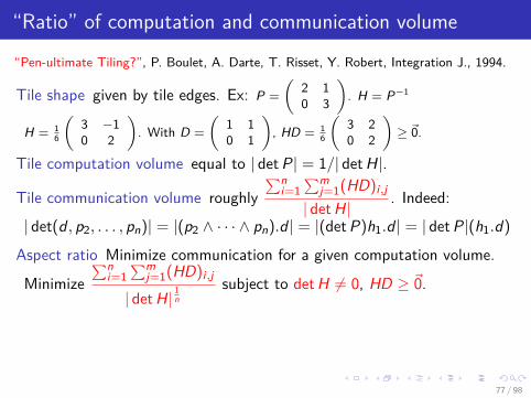

“Ratio” of computation and communication volume
“Pen-ultimate Tiling?”, P. Boulet, A. Darte, T. Risset, Y. Robert, Integration J., 1994.
Tile shape given by tile edges. Ex: P =
(2 10 3
). H = P−1
H = 16
(3 −10 2
). With D =
(1 10 1
), HD = 1
6
(3 20 2
)≥ ~0.
Tile computation volume equal to | detP| = 1/| detH|.
Tile communication volume roughly∑n
i=1∑m
j=1(HD)i ,j
| detH| . Indeed:
| det(d , p2, . . . , pn)| = |(p2 ∧ · · · ∧ pn).d | = |(detP)h1.d | = | detP|(h1.d)
Aspect ratio Minimize communication for a given computation volume.
Minimize∑n
i=1∑m
j=1(HD)i ,j
| detH| 1nsubject to detH 6= 0, HD ≥ ~0. Solvable!
If D is square, non singular, opt. for H = D−1 and ratio n| detD| 1n .General case: cone C(D), opt. for n generators of C∗(D), scaled toinduce the same communication on all faces.
77 / 98

Generating loop bounds for tiled codes“Scanning Polyhedra with DO Loops”, Ancourt, Irigoin, PPoPP’91.“An Efficient Code Generation Technique for Tiled Iteration Spaces”, Goumas, Athanasaki,Koziris, IEEE TPDS, 2003.“Parameterized Tiled Loops for Free”, Renga., Kim, Rajopadhye, Strout, PLDI’07.
Tile of size ~s with origin ~i0: ~i | ~i0 ≤~i ≤ ~i0 +~s −~1.
Elementary bounding box method: many empty tiles.//Original codefor(t=1; t<=M; t++)
for(i=2; i<=N; i++)S(t,i);
//Skewed codefor(t=1; t<=M; t++)
for(k=2+t; k<=N+t; k++)S(t,k-t);
//Tiled code, many empty iterationsfor(T=1; T<=M; T+=st)
for(K=3; K<=N+M; K+=skfor(t=max(T,1); t<=min(T+st-1,M); t++)
for(k=max(K,2+t); k<=min(K+sk-1,N+t); k++)S(t,k-t);
78 / 98

Generating loop bounds for tiled codes“Scanning Polyhedra with DO Loops”, Ancourt, Irigoin, PPoPP’91.“An Efficient Code Generation Technique for Tiled Iteration Spaces”, Goumas, Athanasaki,Koziris, IEEE TPDS, 2003.“Parameterized Tiled Loops for Free”, Renga., Kim, Rajopadhye, Strout, PLDI’07.
Tile of size ~s with origin ~i0: ~i | ~i0 ≤~i ≤ ~i0 +~s −~1.
Exact computation of non-empty tiles for fixed tile sizes.//Original codefor(t=1; t<=M; t++)
for(i=2; i<=N; i++)S(t,i);
//Skewed codefor(t=1; t<=M; t++)
for(k=2+t; k<=N+t; k++)S(t,k-t);
Code not depicted. Only for fixed tile sizes. Express the lattice L(~s) of alltile origins ~i0 = ~0 mod ~s, and project existential variables.
78 / 98

Generating loop bounds for tiled codes“Scanning Polyhedra with DO Loops”, Ancourt, Irigoin, PPoPP’91.“An Efficient Code Generation Technique for Tiled Iteration Spaces”, Goumas, Athanasaki,Koziris, IEEE TPDS, 2003.“Parameterized Tiled Loops for Free”, Renga., Kim, Rajopadhye, Strout, PLDI’07.
Tile of size ~s with origin ~i0: ~i | ~i0 ≤~i ≤ ~i0 +~s −~1.
Approx. iterations ~z | Q~z ≥ ~b by the “outer set” ~z | Q~z + Q+~s ≥ ~b.//Skewed codefor(t=1; t<=M; t++)
for(k=2+t; k<=N+t; k++)S(t,k-t);
Outer set shift:1 ≤ t ≤ M ⇒ 2− st ≤ t ≤ M2 ≤ k−t ≤ N ⇒ 3−sk ≤ k−t ≤ N+st−1
//Tiled code, fewer empty iterationsLBT = 2-st; LBT = ceil(LBT/st)*st;for(T=LBT; T<=M; T+=st)
LBK = 3+t-sk; LBK = ceil(LBK/sk)*sk;for(K=LBK; K<=N+t+st-1; K+=sk
for(t=max(T,1); t<=min(T+st-1,M); t++)for(k=max(K,2+t); k<=min(K+sk-1,N+t); k++)
S(t,k-t);
78 / 98

INTER-TILE DATA REUSE ANDLOCAL STORAGE
79 / 98

General specification of data transfers
DefinitionLoad(T ): data loaded from DDR just before executing tile T .Store(T ): data stored to DDR just after T .In(T ): input data for T , i.e., read before being possibly written in T .Out(T ): output data for T , i.e., data written in T .
Minimal dependence structureTiles
Computes
Loads
Stores
T − 2 T − 1 T + 1 T + 2T
GoalsReuse local data: intra- and inter-tile reuse in a tile strip.Do not store back after each write: external memory not up-to-date.Minimize live-ranges in local memory: need local memory allocation.
80 / 98

Inter-tile data reuse
Global
Local
Load Store Load Store
Comp Comp
81 / 98

Inter-tile data reuse
Global
Local
Load Store Load Store
Comp Comp
81 / 98

Inter-tile data reuse
Global
Local
Load Store Load Store
Comp Comp
81 / 98
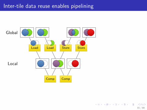
Inter-tile data reuse enables pipelining
Global
Local
Load Load Store Store
Comp Comp
81 / 98

Inter-tile reuse formula w.r.t. a generic tile T
Load(T ) = In(T ) \⋃
T ′<sTIn(T ′) ∪Out(T ′)
j
i0,0
0,1
0,2
0,3
1,0
1,1
1,2
1,3
2,0
2,1
2,2
2,3
3,0
3,1
3,2
3,3
si I ≤ i < si (I + 1)
sjJ ≤ j < sj(J + 1)
i , j ∈ Domain
Quadratic if T indexed by b~i/~sc.
82 / 98

Inter-tile reuse formula w.r.t. a generic tile T
Load(T ) = In(T ) \⋃
T ′<sTIn(T ′) ∪Out(T ′)
j
i0,0
0,3
0,6
0,9
3,0
3,3
3,6
3,9
6,0
6,3
6,6
6,9
9,0
9,3
9,6
9,9
I ≤ i < I + si
J ≤ j < J + sj
i , j ∈ Domain
Affine with tile origin? Not yet.I ≡ 0 (mod si )
J ≡ 0 (mod sj)
82 / 98

Inter-tile reuse formula w.r.t. a generic tile T
Load(T ) = In(T ) \⋃
T ′<sTIn(T ′) ∪Out(T ′)
j
i
Still not affine
82 / 98

Inter-tile reuse formula w.r.t. a generic tile T
Load(T ) = In(T ) \⋃
T ′<sT
⋃x∈T ′
in(x) ∪ out(x)j
i
Piece-wise affine!
82 / 98

Inter-tile reuse formula w.r.t. a generic tile T
Load(T ) = In(T ) \⋃
T ′≺sTIn(T ′) ∪Out(T ′)
j
i
Still piece-wise affine.Computations can be done with iscc.
82 / 98

Approximations: why?
Some operations may executeif conditions that are not analyzable.
Some data may be accessedaccess functions that are not fully analyzable.
Approximated In/Out sets for tiles * In, Out, Out.due to the analysis (e.g., array regions);by choice to represent simpler sets (e.g., hyper-rectangles);to simplify the analysis (e.g., Fourier-Motzkin).
Approximated Load/Store sets * Store, Load.to simplify code generation;to perform communications by blocks;to simplify memory allocation;. . .
83 / 98

May-write approximation hazard
Problem:Tile T may write X, i.e., X ∈ Out(T )
Tile T’ may read X, i.e., X ∈ In(T ′)Only T and T’ may access X
Should we load X? When?
T’ happens before T * load before T’T’ happens after T and X ∈ Out(T ) * do not loadT’ happens after T and X 6∈ Out(T ) * load before T
84 / 98

Reuse formula with approximation and point-wise functions
Load(T ) = F (T ) \⋃
T ′<sTF (T ′)
j
i
F defined at tile level.Can we use the same trick as for theexact case?
* similar to the exact case.
85 / 98

Reuse formula with approximation and point-wise functions
Load(T ) = F (T ) \⋃
T ′≺sTF (T ′)
j
i
Yes if ⋃T ′<sT
F (T ′) =⋃
T ′≺sTF (T ′)
* similar to the exact case.
85 / 98

Reuse formula with approximation and point-wise functions
Load(T ) = F (T ) \⋃
T ′≺sTF (T ′)
j
i
C set of all tiles, C1, C2 ⊆ Csuch that
⋃T∈C1 T =
⋃T∈C2 T⋃
T∈C1F (T )
?=
⋃T∈C2
F (T )
Iff F is point-wise:
∃f ,∀T ∈ C,F (T ) =⋃
x∈Tf (x)
* similar to the exact case.
85 / 98

Reuse formula with approximation and point-wise functions
Load(T ) = F (T ) \⋃
T ′≺sTF (T ′)
j
i
C set of all tiles, C1, C2 ⊆ Csuch that
⋃T∈C1 T =
⋃T∈C2 T⋃
T∈C1F (T )
?=
⋃T∈C2
F (T )
Iff F is point-wise:
∃f ,∀T ∈ C,F (T ) =⋃
x∈Tf (x)
* similar to the exact case.
85 / 98

Simple script with iscc# InputsParams := [M, N, s_1, s_2] -> : s_1 >= 0 and s_2 >= 0 ;Domain := [M, N] -> # Iteration domains
S_1[i_1, i_2] : 1 <= i_2 <= N-2 and 0 <= i_1 <= M-1;S_2[i_1, i_2] : 1 <= i_2 <= N-2 and 0 <= i_1 <= M-1;
* Params;Read := [M, N] -> # Read access functions
S_1[i_1, i_2] -> A[m] : -1 + i_2 <= m <= 1 + i_2;S_2[i_1, i_2] -> B[i_2]; * Domain;
Write := [M, N] -> # Write access functionsS_1[i_1, i_2] -> B[i_2];S_2[i_1, i_2] -> A[i_2]; * Domain;
Theta := [M, N] -> # Preliminary mappingS_1[i_1, i_2] -> [i_1, 2 i_1 + i_2, 0];S_2[i_1, i_2] -> [i_1, 1 + 2 i_1 + i_2, 1]; ;
# Tools for set manipulationsTiling := [s_1, s_2] -> # Two dimensional tiling
[[I_1, I_2] -> [i_1, i_2, k]] -> [i_1, i_2, k] :I_1 <= i_1 < I_1 + s_1 and I_2 <= i_2 < I_2 + s_2 ;
Coalesce := [I_1, I_2] -> [[I_1, I_2] -> [i_1, i_2, k]] ;Strip := [I_1, I_2] -> [I_1, I_2’] ;Prev := # Lexicographic order
[[I_1, I_2] -> [i_1, i_2, k]] -> [[I_1, I_2] -> [i_1’, i_2’, k’]] :i_1’ <= i_1 - 1 or (i_1’ <= i_1 and i_2’ <= i_2 - 1)or (i_1’ <= i_1 and i_2’ <= i_2 and k’ <= k - 1) ;
TiledPrev := [s_1, s_2] -> # Special ‘‘lexicographic’’ order[I_1, I_2] -> [I_1’, I_2’] : I_1’ <= I_1 - s_1 or
(I_1’ <= I_1 and I_2’ <= I_2 - s_2) * Strip;TiledNext := TiledPrev^-1;
# Set/relation computationsTiledRead := Tiling.(Theta^-1).Read;TiledWrite := Tiling.(Theta^-1).Write;In := Coalesce.(TiledRead - (Prev.TiledWrite));Out := Coalesce.TiledWrite;Load := In - ((TiledPrev.In) + (TiledPrev.Out));Store := Out - (TiledNext.Out);print coalesce (Load % Params);print coalesce (Store % Params);
86 / 98

Load/store sets for tiled Jacobi 1D
Load(~I) = A(m) | 1 ≤ m + 2I1 − I2 ≤ s2, s1 ≥ 1, I1 ≥ 0, m ≥ 1, I1 ≤ −1+ M,I2 ≥ 2− s2 + 2I1, m ≤ −1+ N, N ≥ 3
∪ A(m) | m ≥ 1+ I2, m ≥ 1, M ≥ 1, m ≤ −1+ N, I1 ≤ −1,I1 ≥ 1− s1, I2 ≥ 2− s2, N ≥ 3, m ≤ s2 + I2
∪ A(1) | I2 = 1+ 2I1 ∧ 0 ≤ I1 ≤ −1+ M, N ≥ 3, s1 ≥ 1, s2 ≥ 1∪ A(m) | 0 ≤ m ≤ 1, I2 = 1 ≤ s2, 1− s1 ≤ I1 ≤ −1, M ≥ 1, N ≥ 3∪ A(0) | 0 ≤ I1 ≤ M − 1, N ≥ 3, s1 ≥ 1, 1 ≤ I2 − 2I1 ≥ 2− s2∪ A(0) | 1− s1 ≤ I1 ≤ −1, M ≥ 1, N ≥ 3, I2 ≥ 2− s2, I2 ≤ 0
Store(~I) = B(m) | m ≥ 1, m ≥ 2− 2M + s2 + I2, m ≤ −2+ N,I1 ≥ 1− s1, 2 ≤ m + 2s1 + 2I1 − I2 ≤ 1+ s2, s1 ≥ 1
∪ B(m) | m ≥ 1, s1 ≥ 1, m ≤ −2+ N, I1 ≤ −1+ M, m ≤ 1− 2M + s2 + I2,m ≥ 2− 2s1 − 2I1 + I2, I1 ≥ 1− s1, M ≥ 1, m ≥ 2− 2M + I2
∪ A(m) | m ≥ 1, m ≥ 1− 2M + s2 + I2, m ≤ −2+ N,I1 ≥ 1− s1, 1 ≤ m + 2s1 + 2I1 − I2 ≤ s2, s1 ≥ 1
∪ A(m) | m ≥ 1, s1 ≥ 1, m ≤ −2+ N, I1 ≤ −1+ M, m ≤ −2M + s2 + I2,m ≥ 1− 2s1 − 2I1 + I2, I1 ≥ 1− s1, M ≥ 1, m ≥ 1− 2M + I2
87 / 98

Local buffer sizes
Sequential Memory Size Pipelined Memory Sizejacobi-1d-imper
A[2s1 + s2]B[2s1 + s2 − 1]
A[2s1 + 2s2]B[2s1 + 2s2 − 2]
jacobi-2d-imperA[2s1 + s2,min(2s1, s2 + 1) + s3]B[2s1 + s2 − 1,min(2s1, s2 + 1) + s3 − 1]
A[2s1 + s2,min(2s1, s2 + 1) + 2s3]B[2s1 + s2 − 1,min(2s1, s2 + 1) + 2s3 − 2]
seidel-2d
A[
s1 + s2 + 1,min(2s1 + 2, s1 + s2, 2s2 + 2) + s3
]A[
s1 + s2 + 1,min(2s1 + 2, s1 + s2, 2s2 + 2) + 2s3
]gemm
A[s1, s3]B[s3, s2]C[s1, s2]
A[s1, 2s3]B[2s3, s2]C[s1, s2]
floyd-warshall
path[max(k + 1, n − k),max(k + 1, n − k)
]path
[max(k + 1, n − k),max(k + 1, n − k, 2s2)
]
88 / 98

Instance-wise order for sequential and parallel loopsfor(i=0; i<n; i++)
for(j=0; j<n; j++) S: ...T: ...
Total order ≺ defined by a sequential schedule σand lexicographic order.σ(S(i , j)) = (i , j, 0), σ(T (i , j)) = (i , j, 1).O ≺ O′ iff σ(O) <lex σ(O
′).S(i , j) ≺ T (i ′, j ′) iff i < i ′ or (i = i ′ and j ≤ j ′).
for(i=0; i<n; i++) forpar(j=0; j<n; j++)
S: ...T: ...
Partial order ≺, some form of lexicographic order.S(i , j) ≺ T (i ′, j ′) iff i < i ′ or (i = i ′ and j = j ′).
forpar(i = 0; i < n; i++) for(j = 0; j < n; j++)
S: ...T: ...
Partial order ≺, some form of lexicographic order.S(i , j) ≺ T (i ′, j ′) iff (i = i ′ and j ≤ j ′).
89 / 98

More general orders: polyhedral fragment of X10
X10 language developed at IBM, variant at Rice (V. Sarkar)PGAS (partitioned global address space) memory principle.Parallelism of threads: in particular keywords finish, async, clock.No deadlocks by construction but non-determinism.
Polyhedral X10 Yuki, Feautrier, Rajopadhye, Saraswat (PPoPP 2013)Can we analyze the code for data races?
finish for(i in 0..n-1)
S1;async
S2;
Yes. Similar to data-flow analy-sis. Partial order ≺: incompletelexicographic order.
clocked finish for(i in 0..n-1)
S1; advance();clocked async
S2; advance();
Undecidable. Partial order ≺c definedby ~x ≺c ~y iff ~x ≺ ~y or φ(~x) < φ(~y).φ(~x) = # advances before (for ≺) ~x .
90 / 98

Liveness analysis
Uses of liveness analysis:Necessary for memory reuse:
Register allocation: interference graph.Array contraction: conflicting relations.Even wire usage: bitwidth analysis.
Important information for:Communication: live-in/live-out sets (inlining, offloading)Memory footprint (e.g., for cache prediction)Lower/upper bounds on memory usage.
Several variants:Value-based or memory-based analysis.Liveness sets or interference graphs.Control flow graphs (CFG): basic blocks, SSA, SSI, etc.Task graphs, parallel specifications: not really explored so far.
91 / 98
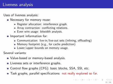

Array contraction: symbolic unrolling, analysis, mapping
x = ...;y = x + ...;... = y;
⇒x = ...;x = x + ...;... = x;
for(i=0; i<n; ++i) for(j=0; j<n; ++j)
A[i][j] = A[i-1][j-1] +A[i-1,j] + A[i-1,j+1];
Mapping: a[i][j] 7→ a[(j-i)%(n+1)]
j
i
for(i=0; i<n; ++i) forpar(j=0; j<n; ++j)
A[i][j] = A[i-1][j-1] +A[i-1,j] + A[i-1,j+1];
Mapping: a[i][j] 7→ a[i%2][j]
j
i
92 / 98

Array contraction: symbolic unrolling, analysis, mapping
c[0] = 0;for(i=0; i<n; i++)
c[i+1] = c[i] + ...;
⇒
c = 0;for(i=0; i<n; i++)
c = c + ...;
for(i=0; i<n; ++i) for(j=0; j<n; ++j)
A[i][j] = A[i-1][j-1] +A[i-1,j] + A[i-1,j+1];
Mapping: a[i][j] 7→ a[(j-i)%(n+1)]
j
i
for(i=0; i<n; ++i) forpar(j=0; j<n; ++j)
A[i][j] = A[i-1][j-1] +A[i-1,j] + A[i-1,j+1];
Mapping: a[i][j] 7→ a[i%2][j]
j
i
92 / 98

Liveness at a given “step” with iscc
# InputsParams := [n] -> : n >= 0 ;Domain := [n] -> S[i,j] : 0 <= i, j < n ;Read := [n] -> S[i,j] -> A[i-1,j-1]; S[i,j] -> A[i-1,j];
S[i,j] -> A[i-1,j+1] * Domain;Write := [n] -> S[i,j] -> A[i,j] * Domain;Sched := [n] -> S[i,j] -> [i,j] ;
# OperatorsPrev := [i,j]->[k,l]: i<k or (i=k and j<l) ;Preveq := [i,j]->[k,l]: i<k or (i=k and j<=l) ;WriteBeforeTStep := (Prev^-1).(Sched^-1).Write;ReadAfterTStep := Preveq.(Sched^-1).Read;
# Liveness and conflictsLive := WriteBeforeTStep * ReadAfterTStep;Conflict := (Live^-1).Live;Delta := deltas Conflict;
*Delta(n) = (1, i1) | i1 ≤ 0, n ≥ 3, i1 ≥ 1− n∪
(0, i1) | i1 ≥ 1− n, n ≥ 2, i1 ≤ −1+ n∪(−1, i1) | i1 ≥ 0, n ≥ 3, i1 ≤ −1+ n
93 / 98

Generalizations? Liveness sets not the right concept
Inner parallelism Almost the same.
Seq/Par nested loops Can use a careful hierarchical approach.Software pipelining Harder to get a concept of “time”.
time step
(L, 2i)
(C , 2i) (L, 2i + 1)
(C , 2i + 1)
(S, 2i + 1)
(S, 2i)
(L, 2i + 3)
(L, 2i + 2)
(C , 2i + 2)
iteration i
time step
(C , i − 1)(L, i)
(S, i − 1)
(C , i)
(L, i + 1)
(S, i)(C , i + 1)
iteration i
On the right, values computed in S(i − 1) and L(i + 1) both conflict withthose in (C , i), but not with each other. Not a clique.
94 / 98

Generalizations? Liveness sets not the right concept
Inner parallelism Almost the same.Seq/Par nested loops Can use a careful hierarchical approach.
Software pipelining Harder to get a concept of “time”.
time step
(L, 2i)
(C , 2i) (L, 2i + 1)
(C , 2i + 1)
(S, 2i + 1)
(S, 2i)
(L, 2i + 3)
(L, 2i + 2)
(C , 2i + 2)
iteration i
time step
(C , i − 1)(L, i)
(S, i − 1)
(C , i)
(L, i + 1)
(S, i)(C , i + 1)
iteration i
On the right, values computed in S(i − 1) and L(i + 1) both conflict withthose in (C , i), but not with each other. Not a clique.
94 / 98
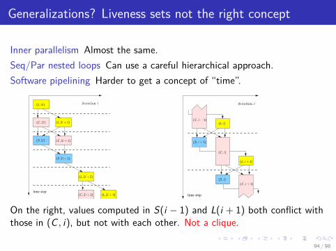
Generalizations? Liveness sets not the right concept
Inner parallelism Almost the same.Seq/Par nested loops Can use a careful hierarchical approach.Software pipelining Harder to get a concept of “time”.
time step
(L, 2i)
(C , 2i) (L, 2i + 1)
(C , 2i + 1)
(S, 2i + 1)
(S, 2i)
(L, 2i + 3)
(L, 2i + 2)
(C , 2i + 2)
iteration i
time step
(C , i − 1)(L, i)
(S, i − 1)
(C , i)
(L, i + 1)
(S, i)(C , i + 1)
iteration i
On the right, values computed in S(i − 1) and L(i + 1) both conflict withthose in (C , i), but not with each other. Not a clique.
94 / 98

Reasoning at the level of traces
Define:a∈ t iff a is executed in a trace t;a≺t b iff a∈ t, b ∈ t and a is executed before b in t;S∃(a, b) iff there is a trace t such that a ≺t b.R∀(a, b) = ¬S∃(b, a) iff, for all traces t, a, b ∈ t implies a ≺t b.
Then, a and b conflict (a ./ b) if, for some trace t, Wa ≺t Wb ≺t Ra.
Conservative approximations for a ./ b:iff S∃(Wa,Ra), S∃(Wa,Wb), S∃(Wb,Ra) iff¬R∀(Ra,Wa), ¬R∀(Wb,Wa), ¬R∀(Ra,Wb).with an under-approximation R∀ ⊆ R∀.
When R∀ is a partial order , a ./ b iff Ra 6≺Wa, Wb 6≺Wa, Ra 6≺Wb .
Wa Ra
Wb
6
6 6
* Covers sequential code, OpenMP-like loop parallelism, OpenMP-4.0 taskparallelism, X10, OpenStream, even some form of if conditions, etc.
95 / 98

Modular mappings and lattices
Modulo mapping ~i 7→ σ(~i) = M~i mod ~b (modulo componentwise).Validity iff ~i ./~j , ~i 6=~j ⇒ σ(~i) 6= σ(~j) iff, with DS = ~i −~j | ~i ./~j,DS ∩ ker σ = ~0.
Lattice An allocation is optimal iff its kernel is a strictly admissible(integer) lattice for DS of minimal determinant (critical lattice).
Integer points
Successive modulo approach.Exhaustive search possible.Upper/lower bounds linked toMinkowski’s theorems, basisreduction, gauge functions.* good order of magnitude ifDS is a polyhedron.
96 / 98

Modular mappings and lattices
Modulo mapping ~i 7→ σ(~i) = M~i mod ~b (modulo componentwise).Validity iff ~i ./~j , ~i 6=~j ⇒ σ(~i) 6= σ(~j) iff, with DS = ~i −~j | ~i ./~j,DS ∩ ker σ = ~0.
Lattice An allocation is optimal iff its kernel is a strictly admissible(integer) lattice for DS of minimal determinant (critical lattice).
0−Symmetric Polytope: vertices (8,1), (−8,−1), (−1,5), and (1,−5)
Successive modulo approach.Exhaustive search possible.Upper/lower bounds linked toMinkowski’s theorems, basisreduction, gauge functions.* good order of magnitude ifDS is a polyhedron.
96 / 98

Modular mappings and lattices
Modulo mapping ~i 7→ σ(~i) = M~i mod ~b (modulo componentwise).Validity iff ~i ./~j , ~i 6=~j ⇒ σ(~i) 6= σ(~j) iff, with DS = ~i −~j | ~i ./~j,DS ∩ ker σ = ~0.
Lattice An allocation is optimal iff its kernel is a strictly admissible(integer) lattice for DS of minimal determinant (critical lattice).Lattice: Basis (9,0), (0,6) Determinant: 54 (i mod 9, j mod 6)
Successive modulo approach.Exhaustive search possible.Upper/lower bounds linked toMinkowski’s theorems, basisreduction, gauge functions.* good order of magnitude ifDS is a polyhedron.
96 / 98

Modular mappings and lattices
Modulo mapping ~i 7→ σ(~i) = M~i mod ~b (modulo componentwise).Validity iff ~i ./~j , ~i 6=~j ⇒ σ(~i) 6= σ(~j) iff, with DS = ~i −~j | ~i ./~j,DS ∩ ker σ = ~0.
Lattice An allocation is optimal iff its kernel is a strictly admissible(integer) lattice for DS of minimal determinant (critical lattice).Lattice: Basis (9,0), (0,5) (i mod 9, j mod 5)Determinant: 45
Successive modulo approach.Exhaustive search possible.Upper/lower bounds linked toMinkowski’s theorems, basisreduction, gauge functions.* good order of magnitude ifDS is a polyhedron.
96 / 98

Modular mappings and lattices
Modulo mapping ~i 7→ σ(~i) = M~i mod ~b (modulo componentwise).Validity iff ~i ./~j , ~i 6=~j ⇒ σ(~i) 6= σ(~j) iff, with DS = ~i −~j | ~i ./~j,DS ∩ ker σ = ~0.
Lattice An allocation is optimal iff its kernel is a strictly admissible(integer) lattice for DS of minimal determinant (critical lattice).
(i−j mod 8, j mod 6)Lattice: Basis (8,0), (6,6) Determinant: 48
Successive modulo approach.Exhaustive search possible.Upper/lower bounds linked toMinkowski’s theorems, basisreduction, gauge functions.* good order of magnitude ifDS is a polyhedron.
96 / 98

Modular mappings and lattices
Modulo mapping ~i 7→ σ(~i) = M~i mod ~b (modulo componentwise).Validity iff ~i ./~j , ~i 6=~j ⇒ σ(~i) 6= σ(~j) iff, with DS = ~i −~j | ~i ./~j,DS ∩ ker σ = ~0.
Lattice An allocation is optimal iff its kernel is a strictly admissible(integer) lattice for DS of minimal determinant (critical lattice).Lattice: Basis (8,0), (4,4) Determinant: 32 (i−j mod 8, j mod 4)
Successive modulo approach.Exhaustive search possible.Upper/lower bounds linked toMinkowski’s theorems, basisreduction, gauge functions.* good order of magnitude ifDS is a polyhedron.
96 / 98

Modular mappings and lattices
Modulo mapping ~i 7→ σ(~i) = M~i mod ~b (modulo componentwise).Validity iff ~i ./~j , ~i 6=~j ⇒ σ(~i) 6= σ(~j) iff, with DS = ~i −~j | ~i ./~j,DS ∩ ker σ = ~0.
Lattice An allocation is optimal iff its kernel is a strictly admissible(integer) lattice for DS of minimal determinant (critical lattice).
Determinant: 32Lattice: Basis (8,0), (3,4) 4i−3j mod 32
Successive modulo approach.Exhaustive search possible.Upper/lower bounds linked toMinkowski’s theorems, basisreduction, gauge functions.* good order of magnitude ifDS is a polyhedron.
96 / 98

Modular mappings and lattices
Modulo mapping ~i 7→ σ(~i) = M~i mod ~b (modulo componentwise).Validity iff ~i ./~j , ~i 6=~j ⇒ σ(~i) 6= σ(~j) iff, with DS = ~i −~j | ~i ./~j,DS ∩ ker σ = ~0.
Lattice An allocation is optimal iff its kernel is a strictly admissible(integer) lattice for DS of minimal determinant (critical lattice).Lattice: Basis (7,0), (4,4) (i−j mod 7, j mod 4)Determinant: 28
Successive modulo approach.Exhaustive search possible.Upper/lower bounds linked toMinkowski’s theorems, basisreduction, gauge functions.* good order of magnitude ifDS is a polyhedron.
96 / 98

Modular mappings and lattices
Modulo mapping ~i 7→ σ(~i) = M~i mod ~b (modulo componentwise).Validity iff ~i ./~j , ~i 6=~j ⇒ σ(~i) 6= σ(~j) iff, with DS = ~i −~j | ~i ./~j,DS ∩ ker σ = ~0.
Lattice An allocation is optimal iff its kernel is a strictly admissible(integer) lattice for DS of minimal determinant (critical lattice).Critical Lattice: Basis (4,3), (8,0) 3i−4j mod 24Determinant: 24
Successive modulo approach.Exhaustive search possible.Upper/lower bounds linked toMinkowski’s theorems, basisreduction, gauge functions.* good order of magnitude ifDS is a polyhedron.
96 / 98
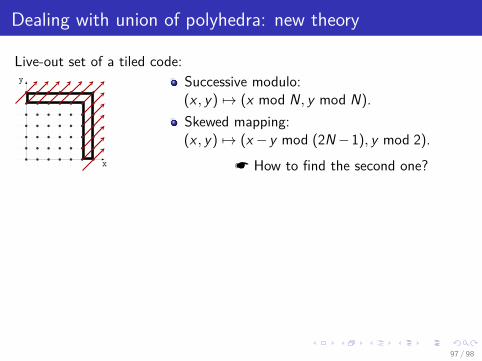
Dealing with union of polyhedra: new theory
Live-out set of a tiled code:
x
y Successive modulo:(x , y) 7→ (x mod N, y mod N).Skewed mapping:(x , y) 7→ (x − y mod (2N−1), y mod 2).
* How to find the second one?
δx
δy
δx
δy
97 / 98

Dealing with union of polyhedra: new theory
Live-out set of a tiled code:
x
y Successive modulo:(x , y) 7→ (x mod N, y mod N).Skewed mapping:(x , y) 7→ (x − y mod (2N−1), y mod 2).
* How to find the second one?
δx
δy
δx
δy
97 / 98
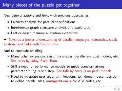
Many pieces of the puzzle get together
New generalizations and links with previous approaches.
Liveness analysis for parallel specifications.Interference graph structure analysis and exploitation.Lattice-based memory allocation extensions.
* Towards a better understanding of parallel languages: semantics, staticanalysis, and links with the runtime.
And to conclude on tiling:Many other extensions exist: tile shapes, parallelism, cost models, etc.See talks by Uday, Sven, Ram.Still a need for performance models to guide transformations,parametric tiling is one step. See talk by Markus on perf. models.Need to integrate user/algorithm freedom. Ex: domain decompositionto define parallel tiles, multipartitioning for ADI codes, etc.
98 / 98