end-of-degree project (tfg)
TRANSCRIPT
END-OF-DEGREE PROJECT (TFG)
TITLE: Theoretical-practical evaluation of the performance of modulation schemes compatible with VLC technology DEGREE: Bachelor’s Degree in Telecommunications systems AUTHOR: Rocío-Zoe Ruiz Ruiz DIRECTOR: Alexis A. Dowhuszko ADVISOR: Luis Alonso Zárate DATE: 24th October 2018


Título: Evaluación teórica-práctica del desempeño de esquemas de modulación compatibles con la tecnología VLC Autor: Rocío-Zoe Ruiz Ruiz Director: Alexis A. Dowhuszko Supervisor: Luis Alonso Zárate Data: 24 de octubre de 2018
Resumen
Las comunicaciones en luz visible son una tecnología que ha emergido en los últimos años proponiendo algunas mejoras respecto a las comunicaciones radio tradicionales. En este proyecto se evalúa la tasa de error de bit de diferentes modulaciones y se describen los requerimientos de las comunicaciones ópticas para ver así cuáles de estas modulaciones pueden ser utilizadas para hacer transmisiones VLC (del inglés, Visible Light Communications). Para ello, el trabajo se ha dividido en tres secciones. En la primera sección se describen los sistemas de comunicaciones en luz visible, así como de las modulaciones que podríamos utilizar, más concretamente de esquemas de modulación basados en OFDM. En la segunda sección, se detallan las simulaciones de MATLAB realizadas, representando la gráfica de la BER de cada uno de los esquemas de modulación, variando un ruido añadido. En la tercera sección se trasladan algunas de las simulaciones a un caso real. Para ello se utilizan dos ordenadores y dos módulos USRP. Un PC hará la función de transmisor y el otro, de receptor. Las USRPs trabajarán como conversores analógico-digital/digital-analógico e irán conectadas entre ellas por un cable que introducirá atenuación. El objetivo de esta configuración será estimar la tasa de error de bit, variando el ruido. Finalmente, se procede a evaluar el sistema sustituyendo el cable que conectaba las dos USRPs con un LED y un fotodetector. De esta manera, se muestra un caso práctico real de un sistema basado en comunicaciones en luz visible, se estudia su desempeño y se presentan las conclusiones.


Title: Theoretical-practical evaluation of the performance of modulation schemes compatible with VLC technology Author: Rocío-Zoe Ruiz Ruiz Supervisor: Alexis A. Dowhuszko Director: Luis Alonso Zárate Date: 24th October 2018
Overview
Visible Light Communications (VLC) is a technology that has emerged in recent years proposing some improvements over traditional radio communications. The objective of this project is to evaluate the bit error rate of different modulations schemes and the requirements of optical communications are described. It is discussed which of them is better to set VLC transmissions. For this, the work has been divided into three sections. The first section describes the communication systems in visible light, as well as the modulations schemes that could be used, more specifically, those that are based on OFDM. In the second section, the MATLAB simulations performed are detailed, representing the bit error rate graph of each of the modulations, varying an added noise. In the third section, the simulations are moved into a real case. For this, two computers and two USRPs modules are used. One of the PC will act as a transmitter and the other as a receiver. The USRPs work as analog-digital/digital-analog converters and are connected to each other by a cable that introduces attenuation. The objective of this configuration is to estimate the bit error rate, varying the noise. Finally, the system is evaluated by replacing the cable that used to connect both USRPs with a LED and a photodetector. In this way, a real practical case of a system based on visible light communications is shown, its performance is studied, and the conclusions are presented.

INDEX
INTRODUCTION ................................................................................................ 1
CHAPTER 1. VISIBLE LIGHT COMMUNICATIONS SYSTEMS ....................... 4
1.1. Introduction ............................................................................ ¡Error! Marcador no definido.
1.2. IEEE 802.15.7 ...................................................................................................................... 5 1.2.1 Modulation methods ............................................................................................... 5 1.2.2 Frame format and dimming methods ..................................................................... 6
1.3. System design of a software defined VLC system ........................................................ 7 1.3.1 Hardware subsystem .............................................................................................. 7 1.3.2 Software subsystem ............................................................................................... 8
1.4. OFDM for Optical communications ................................................................................. 8 1.4.1 Introduction ............................................................................................................. 8 1.4.2 OFDM system description .................................................................................... 10 1.4.3 OFDM applied to OC ............................................................................................ 11 1.4.4 Disadvantages of OFDM ...................................................................................... 13
1.4.4.1 Peak-to-Average Power Ratio ........................................................................... 13 1.4.4.2 Sensitivity to Frequency Offset and Phase Noise ............................................. 14
CHAPTER 2. MATLAB SIMULATIONS .......................................................... 15
2.1. Introduction ...................................................................................................................... 15
2.2. Simulations ...................................................................................................................... 15 2.2.1. BPSK BER Curve ................................................................................................. 15 2.2.2. QPSK/4QAM BER Curve ..................................................................................... 16 2.2.3. QPSK/4QAM BER Curve (using blocks of symbols) ............................................ 17 2.2.4. 16QAM BER Curve .............................................................................................. 19 2.2.5. 16QAM BER Curve (using symbol blocks) ........................................................... 21 2.2.6. Multicarrier IFFT of discrete time domain signal .................................................. 22 2.2.7. IFFT for 16QAM BER and 4QAM BER Curve with different Clipping Ratio (CR) 24 2.2.8. DCO-OFDM for 4QAM BER Curve with different CR........................................... 27
CHAPTER 3. DEMONSTRATION OF A VLC SYSTEM USING USRPS ........ 30
3.1 Introduction ...................................................................................................................... 30
3.2 USRP connection and environment .............................................................................. 30 3.2.1 Introduction to USRP ............................................................................................ 30 3.2.2 USRP Connection ................................................................................................ 31
3.3 Transmitter software implementation ........................................................................... 33 3.3.1 Variables to be set ................................................................................................ 33 3.3.2 Loading MATLAB file with BPSK symbols ........................................................... 33 3.3.3 Adding noise ......................................................................................................... 34 3.3.4 Preamble .............................................................................................................. 34 3.3.5 Matched filter and oversampling........................................................................... 35 3.3.6 Adapting the samples to the LED range ............................................................... 36
3.3.7 Sending the samples ............................................................................................ 37 3.3.8 Complete script ..................................................................................................... 37
3.4 Receiver software implementation ................................................................................ 40 3.4.1 Defined vectors ..................................................................................................... 41 3.4.2 Preamble detection and matched filter ................................................................. 42 3.4.3 Demodulation........................................................................................................ 42 3.4.4 Error counter ......................................................................................................... 42 3.4.5 BER obtaining ....................................................................................................... 43 3.4.6 Complete script ..................................................................................................... 43
3.5 LED Driver Circuit and Photodetector ........................................................................... 47
3.6 Complete system and results ......................................................................................... 48
CONCLUSIONS ............................................................................................... 51
BIBLIOGRAPHY .............................................................................................. 52
APPENDICES .................................................................................................. 54
1.1 USRP Hardware Driver .................................................................................................... 55 1.1.1 Host Computer...................................................................................................... 55 1.1.2 1.1.2 Microsoft Visual Studio Development environment configuration ............... 55 1.1.3 Install Boost boost_1_67_0_b1-msvc-14.1-64.exe for windows .......................... 55 1.1.4 Install the latest UHD ............................................................................................ 56 1.1.5 Setting Environment Variables ............................................................................. 57
1.2 Build the Project in VS2017 ............................................................................................ 59
1.3 USRP Connection ............................................................................................................ 63 1.3.1 Hardware .............................................................................................................. 63 1.3.2 Host computer IP Configuration ........................................................................... 64 1.3.3 Command Checking ............................................................................................. 64 1.3.4 Updating UHD Image Loader ............................................................................... 65

ACRONYMS AND ABBREVIATIONS
ADC Analog-to-Digital Converter ACO-OFDM Asymmetrically Clipped OFDM API Application Programming Interface BER Bit error rate BPSK Binary Phase-Shift Keying CPU Central Processing Unit CR Clipping Ratio CSK Color Shift Keying DAC Digital-to-Analog Converter DDC Digital Down Converter DC Direct Current DCO-OFDM DC-biased Optical OFDM DSP Digital Signal Processor EbNo Energy per Bit to Noise power spectral density ratio FDM Frequency Division Multiplexing FFT Fast Fourier Transform FPGA Field-Programmable Gate Array GPP General Purpose Processor HW Hardware IFFT Inverse Fast Fourier Transform LED Light-Emitting Diode MOSFET Metal-Oxide-Semiconductor Field-Effect Transistor OFDM Orthogonal Frequency-Division Multiplexing OOB Out-Of-Band OOK On-Off Keying OWC Optical Wireless Communications PAPR Peak-to-Peak Average Ratio PC Personal Computer PD Photodetector PPM Pulse Position Modulation PWM Pulse Width Modulation QAM Quadrature Amplitude Modulation QPSK Quadrature Phase-Shift Keying RF Radio Frequency SDR Software Defined Radio SW Software UHD USRP Hardware Driver USRP Universal Software Radio Peripheral VLC Visible Light Communications VPPM Variable Pulse Position Modulation WDM Wave Division Multiplexing
LIST OF FIGURES Figure 1. Main configuration for the real experience .......................................... 2 Figure 2. Position of the visible light range at the electro-magnetic spectrum .... 4 Figure 3. PHY I and PHY II modulation schemes ............................................... 6 Figure 4. VLC frame structure ............................................................................ 6 Figure 5. Spectrum of WDM or FDM signals (a) and OFDM signal (b) .............. 9
Figure 6. Frequency-Time representative of an OFDM signal ............................ 9 Figure 7. Block diagram of an OFDM communication system for RF wireless
applications ............................................................................................... 10 Figure 8. Bipolar and unipolar OFDM signal..................................................... 12 Figure 9. Received 64-QAM constellation in OFDM system with carrier frequency
offset ......................................................................................................... 14
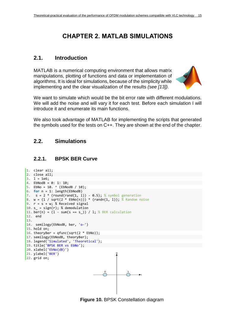
Figure 10. BPSK Constellation diagram ........................................................... 15
Figure 11. BPSK BER vs EbNo ........................................................................ 16 Figure 12. QPSK/4QAM Constellation diagram ................................................ 17 Figure 13. QPSK BER vs EbNo ....................................................................... 17 Figure 14. QPSK/4QAM BER vs EbNo ............................................................ 19
Figure 15. 16QAM Constellation diagram ........................................................ 20 Figure 16. 16QAM BER vs EbNo ..................................................................... 20
Figure 17. 16QAM BER vs EbNo ..................................................................... 22 Figure 18. Real and imaginary part of a discrete IFFT ..................................... 23 Figure 19. Real and imaginary part of a discrete FFT ...................................... 23
Figure 20. 16QAM BER vs EbNo with different CR .......................................... 26 Figure 21. Extracted curve from a paper ............. ¡Error! Marcador no definido. Figure 22. 4QAM real part BER vs EbNo with Hermitian symmetry, Clipping and
bias DC ..................................................................................................... 29
Figure 23. Main diagram of the System ............................................................ 30 Figure 24. USRP N210 ..................................................................................... 31
Figure 25. USRP transmitter (below) and USRP receiver (on the top) ............. 32 Figure 26. Work environment ........................................................................... 32 Figure 27. Random BPSK symbols (initre.txt) .................................................. 34
Figure 28. Raised cosine generated by MATLAB ............................................. 35 Figure 29. Operation region of the LED ............................................................ 36 Figure 30. LED Driver circuit ............................................................................ 47
Figure 31. LED Driver Circuit scheme .............................................................. 47 Figure 32. Photodetector .................................................................................. 48 Figure 33. Complete system in an optimal position .......................................... 49 Figure 34. Comparison between the original file and the symbols received ..... 49
Figure 35. Transmitter cmd .............................................................................. 50 Figure 36. Receiver cmd .................................................................................. 50 Figure 37. Available downloads ........................................................................ 55
Figure 38. UHD installer ................................................................................... 56 Figure 39. Choose 64 bits option ...................................................................... 56
Figure 40. Choose: Do not add UHD to the system PATH ............................... 56 Figure 41. Default destination folder (can be changed) .................................... 57 Figure 42. The file after installation .................................................................. 57 Figure 43. Control panel -> System and Security->System .............................. 57 Figure 44. Click Environment Variables ........................................................... 58 Figure 45. Edit the path .................................................................................... 58

Figure 46. Add the path of UHD\bin. Click OK.................................................. 58
Figure 47. Choose Empty Project. .................................................................... 59
Figure 48. Change to x64 (bits) ........................................................................ 59 Figure 49. Add New Item .................................................................................. 59 Figure 50. Choose C++ File (.cpp) ................................................................... 60 Figure 51. Right click UHD_Test > Properties / View > Property Pages .......... 60 Figure 52. Configuration: Release; Platform: Active(x64) /Active(Win32) for
32bits; C/C++ > General > Additional Include Directories ......................... 60 Figure 53. Click the right triangle, then choose <Edit…> ................................. 61 Figure 54. Add the directory UHD\include > add the directory local\boost_1_67_0
> OK .......................................................................................................... 61 Figure 55. Linker > General > Additional Library Directories ............................ 61
Figure 56. <edit…> > Add the directory UHD\lib > add the directory local\boost_1_67_0\lib64-msvc-14.1 > OK ................................................ 62
Figure 57. Linker > Input > Additional Dependencies > Add uhd.lib; > OK ....... 62 Figure 58. Change to Release .......................................................................... 62 Figure 59. cmd display when USRP is connected ............................................ 64 Figure 60. This command can display the hardware of USRP. For example,
knowing the daughterboard type whether it is LFTX/LFRX. ...................... 64 Figure 61. Updating the firmware of USRP when it is old ................................. 65


Theoretical-practical evaluation of the performance of OFDM modulation schemes compatible with VLC technology 1
INTRODUCTION During the last 100 years, radio communications dominated the world of wireless communication. After the invention of the mobile phone, the popularity of short-range radio communications has increased. More and more mobile devices have appeared with an increasing need to exchange data wirelessly. This massive increasing in the number of mobile devices is provoking a shortage of radio spectrum resources. The efforts of the research community have been redirected toward the exploration of new solutions that could guarantee an efficient usage of the available spectrum. Technics such as cognitive radio, spectrum sharing and, also, optical wireless communications have emerged. Most optical wireless communication (OWC) applications are related to short-range and low-data-rate communications such as infrared light. However, in the last few years visible light communications, a new paradigm of OWC, is being developed. VLC uses beams of light to send information. The main challenge of VLC systems consists of finding a source of artificial light that can be easily modulated. LEDs are a perfect solution due to their cost-effectivity relation. Because of its performance, there is a growing number of application scenarios: hotels, hospitals, traffic lights, in-home applications, among others, where this alternative is replacing incandescent light bulbs and fluorescent lamps. White-LEDs can also be used as transmitters without losing their main functionality as illumination sources, enabling the appearance of VLC. This technology has many advantages when compared to radio-wave communications systems. For example, robustness against electromagnetic interference and a high level of protection against eavesdropping. Industry is also interested in this technology. That is why the number of patents related to VLC is increasing. Due to this interest, centers such as CTTC, are researching on this topic. In 2011, the first IEEE 802.15.7 standard for VLC was published and, few months after that, the CTTC developed one of the first VLC demonstrators in the world using the Software Defined Radio (SDR) concept, where the digital signal processing is performed in a general-purpose processor and the signal acquisition/conversion is done using programmable hardware. The contribution of this TFG has been mainly related to develop a real communication system using OFDM modulation. To begin this project, basics of concepts such as VLC, OFDM, optical OFDM, MATLAB simulations, USRP, USRP hardware driver (UHD) and LEDs were studied. Before starting implementing the real system, some MATLAB simulations were done to analyze the behavior of some of the most important and known
2 Theoretical-practical evaluation of the performance of OFDM modulation schemes compatible with VLC technology
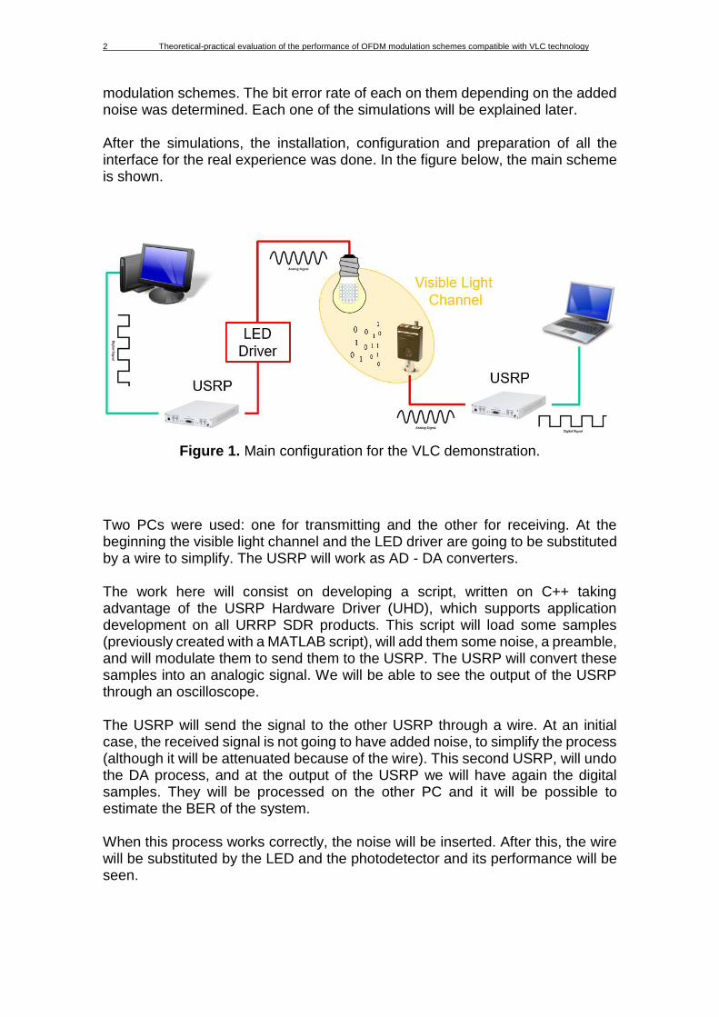
modulation schemes. The bit error rate of each on them depending on the added noise was determined. Each one of the simulations will be explained later. After the simulations, the installation, configuration and preparation of all the interface for the real experience was done. In the figure below, the main scheme is shown.
Figure 1. Main configuration for the VLC demonstration.
Two PCs were used: one for transmitting and the other for receiving. At the beginning the visible light channel and the LED driver are going to be substituted by a wire to simplify. The USRP will work as AD - DA converters. The work here will consist on developing a script, written on C++ taking advantage of the USRP Hardware Driver (UHD), which supports application development on all URRP SDR products. This script will load some samples (previously created with a MATLAB script), will add them some noise, a preamble, and will modulate them to send them to the USRP. The USRP will convert these samples into an analogic signal. We will be able to see the output of the USRP through an oscilloscope. The USRP will send the signal to the other USRP through a wire. At an initial case, the received signal is not going to have added noise, to simplify the process (although it will be attenuated because of the wire). This second USRP, will undo the DA process, and at the output of the USRP we will have again the digital samples. They will be processed on the other PC and it will be possible to estimate the BER of the system. When this process works correctly, the noise will be inserted. After this, the wire will be substituted by the LED and the photodetector and its performance will be seen.

Theoretical-practical evaluation of the performance of OFDM modulation schemes compatible with VLC technology 3
Along this project memory, fundamentals of conventional OFDM (radio systems), optical OFDM and its basic concepts are shown at the first chapter. At the second chapter, the MATLAB simulations done are introduced, and all the scripts and BER graphs are exposed, as well as a brief description. At the third chapter the USRP will be introduced: the configuration and the previous work before implementing a transmission. At the last chapter, how the transmission was done is explained. the most basic one will be shown: based on a BPSK modulation. After this the LED configuration will be discussed and the results of this test will be presented.

4 Theoretical-practical evaluation of the performance of OFDM modulation schemes compatible with VLC technology
CHAPTER 1. VISIBLE LIGHT COMMUNICATIONS SYSTEMS
1.1. Overview to VLC technology
Visible light communications are those OWC systems in which visible lights are applied. The challenge is to find luminaires with an add-on function, which has no negative influence on their illumination functionality. This dual role can be fulfilled with LEDs, which can be used to send high data-rates.
As current-driven semiconductor diodes, LEDs provide a high modulation potential. It offers benefits such as a huge bandwidth in the visible part of the optical electro-magnetic spectrum, the absence of electro-magnetic interference (which exists in radio systems) or the option of create and isolate communication cells with privacy by directing the light to the working area (see [1]).
The research community is now focused on developing demonstrators capable of providing the feasibility of this technology for wireless applications. Based on the modulation technique used for transmitting the information, we find:
- Binary-level modulation. Information is sent in each symbol period through the variation of two intensity levels. They have simple and cheap implementations. Non-return-to-zero or on-off keying are examples. They can achieve 40Mb/s.
- Multi-level modulation. Information is sent by modifying the intensity values in a continuous range or using predefined values. They provide
Figure 2. Position of the visible light range at the electro-magnetic spectrum (see [2])

Theoretical-practical evaluation of the performance of OFDM modulation schemes compatible with VLC technology 5
better usage of the available bandwidth, so they can achieve higher data rates.
The results are obtained in special conditions, and in most cases the range of the wireless link is on the order of ten centimeters. Nevertheless, it can become a complementary technology for wireless communications.
1.2. IEEE 802.15.7 standard
Aware of the potential of VLC the research community provided a framework for defining VLC communications. The first release was published in September 2011 and presents rules for the implementation of VLC systems having two main functionalities: illumination and data communications (see [3] and [4]). In this specifications, physical and media access control layers for short-range optical wireless communications using visible light for indoor and outdoor applications are defined. IEEE 802.15.7 also pays attention to problems related to illumination systems such as flicker mitigation, related to eye safety regulations, or dimming support, related to power savings and energy efficiency.
1.2.1 Modulation methods used in IEEE 802.15.7
There are three PHY layer types grouped by data rate according to IEEE 805.15.7:
PHY I 11.67 – 266.6 kb/s OOK
PHY II 1.25 – 96 Mb/s VPPM
PHY III 12 – 96 Mb/s CSK
Table 1. Supported data rated in each PHY and modulation formats used The modulation used in PHY I and PHY II are OOK and variable pulse position modulation (VPPM), which is a combination of two-pulse position modulation and pulse width modulation (for dimming support). PHY III uses a particular modulation format called color shift keying, where multiple optical sources are combined to produce white light. In OOK, the simplest modulation a rectangular pulse is transmitted during a fixed time slot if the coded bit is “1” or there is an absence of pulse if the coded bit is “0”.

6 Theoretical-practical evaluation of the performance of OFDM modulation schemes compatible with VLC technology
On the other hand, PPM is a modulation technique that uses rectangular pulse to code bits of information. The width of the pulse in time is smaller that the complete slot and the position of the pulse inside the transmission time slot is used. For example, in 2PPM, two pulses are used to encode the information bits. If a “0” is transmitted, the pulse is aligned with the beginning of the transmission slot and if a “1” is transmitted, with the end (see [6]). The standard is designed to work in scenarios with the presence of optical noise sources (natural or artificial). PHY I is good for low-rate/long-distance, so, outdoor applications and PHY II is optimized for high-rate/short-distances; indoor applications. Different forward error correction schemes are included in each PHY layer definition, derived from the necessity to work in different scenarios. For outdoor applications we find more resilient codes to counter-act day light interference.
1.2.2 Frame format and dimming methods
The frame defined by the specifications at the physic level has three elements: the synchronization header, the physical header and the physical service data unit.
Dimming is a feature present in current illumination systems that allows the user to control the brightness/dimming level on the light source. It is necessary to preserve all the functionality of the illumination system (see [7]).
Figure 3. PHY I and PHY II modulation schemes (see [5])
Figure 4. VLC frame structure

Theoretical-practical evaluation of the performance of OFDM modulation schemes compatible with VLC technology 7
For the OOK modulation, we have two options. The first one consists on redefining the “ON” and “OFF” levels to achieve the desired brightness. The second option is to insert compensation symbols. The disadvantage of this second method is that the data rate decreases proportionally to the number of compensation symbols. VPPM allows dimming control due to its PWM characteristics. The dimming is adjusted by changing the “ON” time pulse width according to the requested dimming level. When data is not being sent, the dimming must be maintained. We can insert idle patterns between data frames, that do not contain information.
1.3. System design of a software defined VLC system
To introduce this new standard into the market we should design a flexible system. For this type of implementation, it is preferred a reconfigurable hardware, but it is required to have high specialized personalization. That is why we use software techniques based on the concept of Software Defined Radio (SDR). The signal processing functions are performed in a general-purpose processor, while the RF and signal conversion (A/D, D/A) are performed in a programmable hardware. The hardware problems are turned into software problems and it needs less specialized personnel.
1.3.1 Hardware subsystem
Generally, in SDR, the interface between HW and SW subsystems is done with the help of specialized devices that provide functionalities like data conversion and data buffering. In this project I chose the commercial platform Universal Software Radio Peripheral (USRP) because of its trade-off between price and performance. USRP are built around a field programmable gate array (FPGA) that includes powerful A/D and D/A converters. The manufacturer is Ettus Research. The complete system includes these two USRP platforms, an amplification stage, the LED driver circuit, and a commercial white LED as a light source (see [8]). The stream of bits generated at the output of the transmitter software subsystem are delivered through a Gigabit/Ethernet Link to the USRP, where they are D/A converted. The modulated signal provided by the SDR platform has a low-level voltage and it must be amplified to control the LED driver circuit. The light intensity generated by LEDs is proportional to the driving current, so, the driver circuit should be able to control this current. At the receiver side, we use a photodetector. We need to process the signal collected by the photodetector first. Then, it delivers the received signal to the USRP receiving platform. There, the

8 Theoretical-practical evaluation of the performance of OFDM modulation schemes compatible with VLC technology
signal is sampled and passed to the receiving computer, where the demodulation is performed.
1.3.2 Software subsystem
The modulation/demodulation of the incoming bits to/from the USRP are performed in a GPP by means of a signal processing open source library. The USRP hardware driver (UHD) is the device driver provided by Ettus Research to use with the USRP. It supports Linux, MacOS, and Windows operative systems. The functionality provided by UHD can be accessed directly with the UHD API, which provides native support for C++. Any other language that can import C++ functions can also use UHD. In our case, we worked on Visual Studio 2017 programming in C++ with the tools of UHD. The software subsystem generates samples and modulates them in function of the chosen modulation. Then it adds a preamble for a simpler detection of the frame in reception.
1.4. OFDM for Optical communications
1.4.1 Introduction
Orthogonal frequency division multiplexing is used in wireless communications due to its effectiveness against intersymbol interference (ISI) caused by a dispersive channel. For example, when the received signal at any time depends on multiple transmitted symbols (like QAM). OFDM has another advantage regarding other techniques: it transfers the complexity of transmitters and receivers from the analog to the digital domain. Because of these advantages, OFDM has been considered for optical communications (see [8]). In OFDM, data is transmitted in parallel on a number of different frequencies, and as a result, the symbol period is much longer than for a serial system. In most of OFDM implementations any residual ISI is removed by using a form of guard interval called cyclic prefix. In OFDM the subcarrier frequencies are chosen so that the signals are mathematically orthogonal over one OFDM period symbol, unlike frequency division multiplexing (FDM) or wavelength division multiplexing (WDM), where information is transmitted on a number of different frequencies simultaneously.

Theoretical-practical evaluation of the performance of OFDM modulation schemes compatible with VLC technology 9
Modulation and multiplexing are achieved digitally using an inverse fast Fourier transform (IFFT). The required orthogonal signals can be generated in a very efficient computationally way (see [9]). In OFDM the spectra of individual subcarriers overlap, but because of the orthogonality property, the subcarriers can be demodulated without interference and without the need of analog filtering to separate the received subcarriers.
Demodulation and demultiplexing are performed by a fast Fourier transform (FFT). The spectrum of an individual OFDM subcarrier has a |sin(x)/x|2 form, so each OFDM subcarrier has significant sidelobes over a frequency range which includes many other subcarriers. A disadvantage of OFDM is the quite sensitivity to frequency offset and phase noise.
Figure 5. Spectrum of WDM or FDM signals (a) and OFDM signal (b)
Figure 6. Frequency-Time representative of an OFDM signal
10 Theoretical-practical evaluation of the performance of OFDM modulation schemes compatible with VLC technology
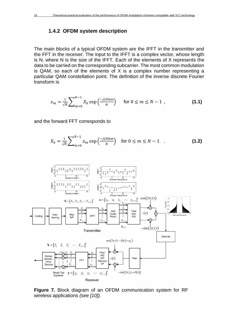
1.4.2 OFDM system description
The main blocks of a typical OFDM system are the IFFT in the transmitter and the FFT in the receiver. The input to the IFFT is a complex vector, whose length is N, where N is the size of the IFFT. Each of the elements of X represents the data to be carried on the corresponding subcarrier. The most common modulation is QAM, so each of the elements of X is a complex number representing a particular QAM constellation point. The definition of the inverse discrete Fourier transform is
𝑥𝑚 =1
√𝑁∑ 𝑋𝑘 exp (
−𝑗2𝛱𝑘𝑚
𝑁)
𝑁−1
𝑚=0 for 0 ≤ 𝑚 ≤ 𝑁 − 1 , (1.1)
and the forward FFT corresponds to
𝑋𝑘 =1
√𝑁∑ 𝑥𝑚 exp (
−𝑗2𝛱𝑘𝑚
𝑁)
𝑁−1
𝑚=0 for 0 ≤ 𝑚 ≤ 𝑁 − 1 . (1.2)
Figure 7. Block diagram of an OFDM communication system for RF wireless applications (see [10]).
Theoretical-practical evaluation of the performance of OFDM modulation schemes compatible with VLC technology 11
The discrete signals at the input and at the output of the transform for each symbol have the same total energy and the same average power. The performance of OFDM systems depend on the average noise power, unlike conventional serial optical systems where it is the peak values of noise which often limit performance. At the output of the IFFT we have a sequence of OFDM symbols. In some OFDM systems we add a cyclic prefix to eliminate ISI and intercarrier interference (ICI). CP is a number of samples from the end of the symbol appended to the start of the symbol. It introduces some redundancy. The first two blocks in the transmitter are the interleaving and coding. They are necessary because if there is frequency selective fading in the channel, some of the parallel data streams will experience deep fading. After it the data is mapped onto complex number representing a constellation. We can also upsample the digital signal before the digital to analog conversion to ease the analog filtering. The signal x(t) is a complex signal which arrives to the input of an IQ modulator for upconversion to the carrier frequency (in wireless systems). Sometimes, for example in optical communications like our system, we need the signal to be real. To get this characteristic, the input to the transmitter IFFT must have Hermitian symmetry:
𝑋𝑁−𝑘 = 𝑋𝑘 ∗ (1.3) At the output of the IFFT, we obtain a cancellation of the imaginary part. When the signal arrives to the receiver, it is downconverted by mixing with in-phase and quadrature components of a locally generated carrier. It should be identical to the carried frequency of the received signal, but, due to error at the carrier recovery at the receive, there may be some difference. Constant errors in the absolute phase are unimportant because they can be compensated by a single tap equalizer, but any frequency error or phase noise can cause problems.
1.4.3 OFDM applied to OC
OFDM has recently been applied to optics communications because of the many advantages. There is an obstacle to adapt classic OFDM: the differences between both systems. In typical (radio) OFDM systems, the bits are carried on the electrical field, so the signal can have positive and negative values (bipolar). At the receiver there is a local oscillator and it is used coherent reception.

12 Theoretical-practical evaluation of the performance of OFDM modulation schemes compatible with VLC technology
Optical systems are usually intensity-modulated and direct-detection. For this, information is carried on the intensity of the optical signal and it can only be positive (unipolar). There are two ways of classifying optical OFDM solutions: by intensity modulation (mainly optical wireless, multimode fiber systems and plastic optical fiber systems) or by linear field modulation (single mode fiber). Because we are interested on optical wireless, we will focus on intensity modulation. The OFDM signal must be represented as intensity. This means that that the modulating signal must be real and positive, while baseband OFDM signals are complex and bipolar. There are two forms of unipolar OFDM: dc-biased optical OFDM (DCO-OFDM), where DC bias is added to the signal and asymmetrically clipped OFDM (ACO-OFDM), where the bipolar OFDM signal is clipped at the zero level. In DCO-OFDM there is a drawback. The PAPR of the OFDM signal some negative peaks of the signal will be clipped and the resulting distortion will limit performance, even with a large bias. PAPR will be described in the next section. In ACO-OFDM, all negative going signals are removed. If only the odd frequency OFDM subcarriers are not zero at the IFFT input, all of the clipping noise falls on the even subcarriers, and the data carrying odd subcarriers are not damaged. ACO-OFDM requires a lower average optical power for a given BER and data rate than DCO-OFDM. Although its greater effectiveness, we will simulate DCO-OFDM on MATLAB due to its simplicity (see [11]).
Figure 8. Bipolar and unipolar OFDM signal
Theoretical-practical evaluation of the performance of OFDM modulation schemes compatible with VLC technology 13
1.4.4 Disadvantages of OFDM
1.4.4.1 Peak-to-Average Power Ratio
The peak-to-average power ratio is the peak power divided by the average power.
𝑃𝐴𝑃𝑅𝑑𝐵 = 10log10|𝑥𝑝𝑒𝑎𝑘|2
𝑥𝑟𝑚𝑠2 (1.4)
Many of the components in the transmitter and receiver should have a wide dynamic range so that the signal is not distorted. Intermodulation got from any nonlinearity results in two main problems: out-of-band (OOB) power and in-band distortion. The specifications on OOB power are very strict because of the near-far problem. The signal samples at the output of the IFFT have Gaussian distributions. This is because this operation is carried out by summing many independently modulated subcarriers. Although OFDM has high signal peaks, they occur rarely. Despite of it, they can cause significant OOB power when the output amplifier is nonlinear or when the amplifier or other components saturate. The clipping ratio is defined as:
𝐶𝑅 = 20 log10𝐴
𝜎 𝑑𝐵 (1.5)
where A is the maximum amplitude and 𝜎2 is the power of x(t). Clipping causes the constellation to shrink and also adds a noise like distortion. There are three main techniques to fight against PAPR: coding techniques, where they code the input vector X so that OFDM symbol which have high PAPR are not used; multiple signal representation, that generate a number of possible transmit signals for each input data sequence and use the one with less PAPR, and, finally, the ones that involve not linear distortion such as clipping.
𝑥𝑐𝑙𝑖𝑝(𝑡) = {𝑥(𝑡), 𝑥(𝑡) < 𝐴
𝐴𝑒𝑗𝑎𝑟𝑔(𝑥(𝑡)), 𝑥(𝑡) ≥ 𝐴 (1.6)
As we see in the previous formula, clipping consists in leaving the original signal while it is lower than a maximum amplitude and, in the rest of the cases, modify it for the maximum amplitude value without losing the imaginary part.
14 Theoretical-practical evaluation of the performance of OFDM modulation schemes compatible with VLC technology
Clipping can be performed on either the analog signal, or an upsampled version of the digital signal with an oversampling. This is because once the signal is D/A converted the peaks of the signal may occur between the discrete samples.
1.4.4.2 Sensitivity to Frequency Offset and Phase Noise
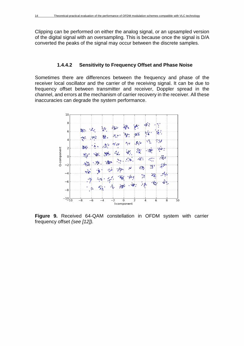
Sometimes there are differences between the frequency and phase of the receiver local oscillator and the carrier of the receiving signal. It can be due to frequency offset between transmitter and receiver, Doppler spread in the channel, and errors at the mechanism of carrier recovery in the receiver. All these inaccuracies can degrade the system performance.
Figure 9. Received 64-QAM constellation in OFDM system with carrier frequency offset (see [12]).
Theoretical-practical evaluation of the performance of OFDM modulation schemes compatible with VLC technology 15
CHAPTER 2. MATLAB SIMULATIONS
2.1. Introduction
MATLAB is a numerical computing environment that allows matrix manipulations, plotting of functions and data or implementation of algorithms. It is ideal for simulations, because of the simplicity while implementing and the clear visualization of the results (see [13]). We want to simulate which would be the bit error rate with different modulations. We will add the noise and will vary it for each test. Before each simulation I will introduce it and enumerate its main functions. We also took advantage of MATLAB for implementing the scripts that generated the symbols used for the tests on C++. They are shown at the end of the chapter.
2.2. Simulations
2.2.1. BPSK BER Curve
1. clear all; 2. close all; 3. l = 1e6; 4. EbNodB = 0: 1: 10; 5. EbNo = 10. ^ (EbNodB / 10); 6. for n = 1: length(EbNodB) 7. s = 2 * (round(rand(1, l)) - 0.5); % symbol generation 8. w = (1 / sqrt(2 * EbNo(n))) * (randn(1, l)); % Random noise 9. r = s + w; % Received signal 10. s_ = sign(r); % demodulation 11. ber(n) = (l - sum(s == s_)) / l; % BER calculation 12. end 13. 14. semilogy(EbNodB, ber, 'o-') 15. hold on; 16. theoryBer = qfunc(sqrt(2 * EbNo)); 17. semilogy(EbNodB, theoryBer); 18. legend('Simulated', 'Theoretical'); 19. title('BPSK BER vs EbNo'); 20. xlabel('EbNo(dB)') 21. ylabel('BER') 22. grid on;
Figure 10. BPSK Constellation diagram

16 Theoretical-practical evaluation of the performance of OFDM modulation schemes compatible with VLC technology
For plotting this curve, we sweep the EbNo (dB) from 0 to 10. We generate random bits and we contaminate them with noise (previously calculated with the linear EbNo). After it, we demodulate the bits contaminated by noise and we estimate the BER by dividing the errors by the total bits transmitted. At the plot we can see both curves: the simulated one and the theorical.
2.2.2. QPSK/4QAM BER Curve
1. clear all; 2. close all; 3. l = 1e6; 4. EbNodB = 0: 1: 10; 5. EbNo = 10. ^ (EbNodB / 10); 6. for n = 1: length(EbNodB); 7. si = 2 * (round(rand(1, l)) - 0.5); % In - phase symbol generation 8. sq = 2 * (round(rand(1, l)) - 0.5); % Quadrature symbol generation 9. s = si + j * sq; 10. w = (1 / sqrt(2 * EbNo(n))) * (randn(1, l) + j * randn(1, l)); % Random noise 11. r = s + w; % Received signal 12. si_ = sign(real(r)); % In - phase demodulation 13. sq_ = sign(imag(r)); % Quadrature demodulation 14. ber1 = (l - sum(si == si_)) / l; % In - phase BER calculation 15. ber2 = (l - sum(sq == sq_)) / l; % Quadrature BER calculation 16. ber(n) = mean([ber1 ber2]); % Overall BER 17. end 18. semilogy(EbNodB, ber, 'o-') 19. hold on; 20. theoryBer = qfunc(sqrt(2 * EbNo)); 21. semilogy(EbNodB, theoryBer); 22. legend('Simulated', 'Theoretical'); 23. title('QPSK BER vs EbNo'); 24. xlabel('EbNo(dB)') 25. ylabel('BER')
grid on;
Figure 11. BPSK BER vs EbNo

Theoretical-practical evaluation of the performance of OFDM modulation schemes compatible with VLC technology 17
In this case, we need to generate symbols with real and imaginary part to recreate the QPSK constellation in equal parts. Then we apply the same procedure as before but considering that we must contaminate both imaginary and real part, so the noise is also going to be imaginary.
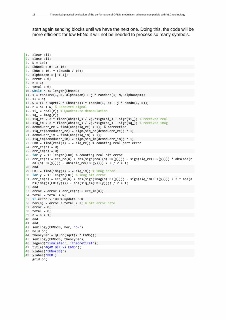
2.2.3. QPSK/4QAM BER Curve (using blocks of symbols)
In this script, we are going to plot the same as in the previous section. The difference will be on the way of writing the script. We will do it in a more realistic form. We will send symbol blocks (thousand in thousand), and we will stop sending them when we have the BER of each EbNo. When we have it we will
Figure 12. QPSK/4QAM Constellation diagram
Figure 13. QPSK BER vs EbNo
18 Theoretical-practical evaluation of the performance of OFDM modulation schemes compatible with VLC technology
start again sending blocks until we have the next one. Doing this, the code will be more efficient: for low EbNo it will not be needed to process so many symbols.
1. clear all; 2. close all; 3. N = 1e3; 4. EbNodB = 0: 1: 10; 5. EbNo = 10. ^ (EbNodB / 10); 6. alpha4qam = [-1 1]; 7. error = 0; 8. n = 1; 9. total = 0; 10. while n <= length(EbNodB) 11. s = randsrc(1, N, alpha4qam) + j * randsrc(1, N, alpha4qam); 12. s1 = s; 13. w = (1 / sqrt(2 * EbNo(n))) * (randn(1, N) + j * randn(1, N)); 14. r = s1 + w; % Received signal 15. si_ = real(r); % Quadrature demodulation 16. sq_ = imag(r); 17. siq_re = 2 * floor(abs(si_) / 2).*sign(si_) + sign(si_); % received real 18. siq_im = 2 * floor(abs(sq_) / 2).*sign(sq_) + sign(sq_); % received imag 19. demoduerr_re = find(abs(siq_re) > 1); % correction 20. siq_re(demoduerr_re) = sign(siq_re(demoduerr_re)) * 1; 21. demoduerr_im = find(abs(siq_im) > 1); 22. siq_im(demoduerr_im) = sign(siq_im(demoduerr_im)) * 1; 23. EBR = find(real(s) ~ = siq_re); % counting real part error 24. err_re(n) = 0; 25. err_im(n) = 0; 26. for y = 1: length(EBR) % counting real bit error 27. err_re(n) = err_re(n) + abs(sign(real(s(EBR(y)))) - sign(siq_re(EBR(y)))) * abs(abs(r
eal(s(EBR(y)))) - abs(siq_re(EBR(y)))) / 2 / 2 + 1; 28. end 29. EBI = find(imag(s) ~ = siq_im); % imag error 30. for y = 1: length(EBI) % imag bit error 31. err_im(n) = err_im(n) + abs(sign(imag(s(EBI(y)))) - sign(siq_im(EBI(y)))) / 2 * abs(a
bs(imag(s(EBI(y)))) - abs(siq_im(EBI(y)))) / 2 + 1; 32. end 33. error = error + err_re(n) + err_im(n); 34. total = total + N; 35. if error > 100 % update BER 36. ber(n) = error / total / 2; % bit error rate 37. error = 0; 38. total = 0; 39. n = n + 1; 40. end 41. end 42. semilogy(EbNodB, ber, 'o-') 43. hold on; 44. theoryBer = qfunc(sqrt(2 * EbNo)); 45. semilogy(EbNodB, theoryBer); 46. legend('Simulated', 'Theoretical'); 47. title('4QAM BER vs EbNo'); 48. xlabel('EbNo(dB)') 49. ylabel('BER')
grid on;

Theoretical-practical evaluation of the performance of OFDM modulation schemes compatible with VLC technology 19
2.2.4. 16QAM BER Curve
1. clear all; 2. close all; 3. l = 1e5; 4. EbNodB = 0: 1: 12; 5. EbNo = 10. ^ (EbNodB / 10); 6. alpha16qam = [-3 - 1 1 3]; 7. for n = 1: length(EbNodB) s = randsrc(1, l, alpha16qam) + j * randsrc(1, l, alpha16qa
m); 8. s1 = (1 / sqrt(10)) * s; 9. w = (1 / sqrt(2 * EbNo(n) * 4)) * (randn(1, l) + j * randn(1, l)); 10. r = s1 + w; % Received signal 11. si_ = real(r) * sqrt(10); 12. sq_ = imag(r) * sqrt(10); % Quadrature demodulation 13. siq_re = 2 * floor(abs(si_) / 2).*sign(si_) + sign(si_); 14. siq_im = 2 * floor(abs(sq_) / 2).*sign(sq_) + sign(sq_); 15. demoduerr_re = find(abs(siq_re) > 3); 16. siq_re(demoduerr_re) = sign(siq_re(demoduerr_re)) * 3; 17. demoduerr_im = find(abs(siq_im) > 3); 18. siq_im(demoduerr_im) = sign(siq_im(demoduerr_im)) * 3; 19. EBR = find(real(s) ~ = siq_re); 20. err_re(n) = 0; 21. err_im(n) = 0; 22. for y = 1: length(EBR) 23. err_re(n) = err_re(n) + abs(sign(real(s(EBR(y)))) - sign(siq_re(EBR(y)))) * abs(abs(r
eal(s(EBR(y)))) - abs(siq_re(EBR(y)))) / 2 / 2 + 1; 24. end 25. EBI = find(imag(s) ~ = siq_im); 26. for y = 1: length(EBI) 27. err_im(n) = err_im(n) + abs(sign(imag(s(EBI(y)))) - sign(siq_im(EBI(y)))) / 2 * abs(a
bs(imag(s(EBI(y)))) - abs(siq_im(EBI(y)))) / 2 + 1; 28. end 29. error(n) = err_re(n) + err_im(n); 30. end 31. ber = error / l / 4; 32. semilogy(EbNodB, ber, 'o-') 33. hold on;
Figure 14. QPSK/4QAM BER vs EbNo

20 Theoretical-practical evaluation of the performance of OFDM modulation schemes compatible with VLC technology
34. theoryBer = 3 / 8 * erfc(sqrt(2 / 5 * EbNo)); 35. semilogy(EbNodB, theoryBer); 36. legend('Simulated', 'Theoretical'); 37. title('16QAM BER vs EbNo'); 38. xlabel('EbNo(dB)') 39. ylabel('BER')
grid on; Here, we plotted the curve of the 16QAM BER. We need a vector [-3, -1, 1, 3], which are the points, in the imaginary and real axis, of the constellation. We generate a stream of symbols of length 1e5. We are using grey code to represent each point at the constellation. As we can see in figure 13, there is only one bit different between adjacent points in the constellation. This is like this because, when noise is high enough and the obtained symbol exceeds the threshold there is only one-bit error. It is very unusual that the bit goes much far away from the adjacent constellation point, and if it is like this and it is very frequent, it means that the system has a very bad quality.
Figure 15. 16QAM Constellation diagram
Figure 16. 16QAM BER vs EbNo

Theoretical-practical evaluation of the performance of OFDM modulation schemes compatible with VLC technology 21
2.2.5. 16QAM BER Curve (using symbol blocks)
1. clear all; 2. close all; 3. block = 1e3; 4. EbNodB = 0: 1: 14; 5. EbNo = 10. ^ (EbNodB / 10); 6. alpha16qam = [-3 - 1 1 3]; 7. error = 0; 8. n = 1; 9. total = 0; 10. while n <= length(EbNodB) 11. s = randsrc(1, block, alpha16qam) + j * randsrc(1, block, alpha16qam); 12. s1 = (1 / sqrt(10)) * s; 13. w = (1 / sqrt(2 * EbNo(n) * 4)) * (randn(1, block) + j * randn(1, block)); 14. r = s1 + w; % Received signal 15. si_ = real(r) * sqrt(10); 16. sq_ = imag(r) * sqrt(10); % Quadrature demodulation 17. siq_re = 2 * floor(abs(si_) / 2).*sign(si_) + sign(si_); % received real part signal 18. siq_im = 2 * floor(abs(sq_) / 2).*sign(sq_) + sign(sq_); % imag part 19. demoduerr_re = find(abs(siq_re) > 3); % correction 20. siq_re(demoduerr_re) = sign(siq_re(demoduerr_re)) * 3; 21. demoduerr_im = find(abs(siq_im) > 3); 22. siq_im(demoduerr_im) = sign(siq_im(demoduerr_im)) * 3; 23. EBR = find(real(s) ~ = siq_re); % counting real part error 24. err_re(n) = 0; 25. err_im(n) = 0; 26. for y = 1: length(EBR) % counting real bit error 27. err_re(n) = err_re(n) + abs(sign(real(s(EBR(y)))) - sign(siq_re(EBR(y)))) * abs(abs(r
eal(s(EBR(y)))) - abs(siq_re(EBR(y)))) / 2 / 2 + 1; 28. end 29. EBI = find(imag(s) ~ = siq_im); % imag error 30. for y = 1: length(EBI) % imag bit error 31. err_im(n) = err_im(n) + abs(sign(imag(s(EBI(y)))) - sign(siq_im(EBI(y)))) / 2 * abs(a
bs(imag(s(EBI(y)))) - abs(siq_im(EBI(y)))) / 2 + 1; 32. end 33. error = error + err_re(n) + err_im(n); 34. total = total + block; 35. if error > 50 % update BER 36. ber(n) = error / total / 4; % bit error rate 37. error = 0; 38. total = 0; 39. n = n + 1; 40. end 41. end 42. semilogy(EbNodB, ber, 'o-') 43. hold on; 44. theoryBer = 3 / 8 * erfc(sqrt(2 / 5 * EbNo)); 45. semilogy(EbNodB, theoryBer); 46. legend('Simulated', 'Theoretical'); 47. title('16QAM BER vs EbNo'); 48. xlabel('EbNo(dB)') 49. ylabel('BER')
grid on; As in the QPSK case, we will change the code to assure we obtain enough errors to estimate the bit error rate (when energy per bit or symbol is very large in relation to the channel noise). It is also much more efficient.
22 Theoretical-practical evaluation of the performance of OFDM modulation schemes compatible with VLC technology
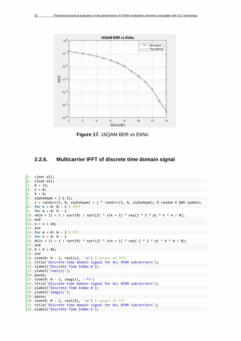
2.2.6. Multicarrier IFFT of discrete time domain signal
1. clear all; 2. close all; 3. N = 32; 4. x = 0; 5. X = 0; 6. alpha4qam = [-1 1]; 7. s = randsrc(1, N, alpha4qam) + j * randsrc(1, N, alpha4qam); % random 4 QAM symbols 8. for k = 0: N - 1 % IFFT 9. for m = 0: N - 1 10. xm(m + 1) = 1 / sqrt(N) / sqrt(2) * s(k + 1) * exp(j * 2 * pi * k * m / N); 11. end 12. x = x + xm; 13. end 14. for m = 0: N - 1 % FFT 15. for k = 0: N - 1 16. XK(k + 1) = 1 / sqrt(N) * sqrt(2) * x(m + 1) * exp(-j * 2 * pi * k * m / N); 17. end 18. X = X + XK; 19. end 20. stem(0: N - 1, real(x), '-o') % output of IFFT 21. title('Discrete time domain signal for ALL OFDM subcarriers'); 22. xlabel('Discrete Time Index m'); 23. ylabel('real(x)'); 24. pause; 25. stem(0: N - 1, imag(x), '-*r') 26. title('Discrete time domain signal for ALL OFDM subcarriers'); 27. xlabel('Discrete Time Index m'); 28. ylabel('imag(x)'); 29. pause; 30. stem(0: N - 1, real(X), '-o') % output of FFT 31. title('Discrete time domain signal for ALL OFDM subcarriers'); 32. xlabel('Discrete Time Index k');
Figure 17. 16QAM BER vs EbNo

Theoretical-practical evaluation of the performance of OFDM modulation schemes compatible with VLC technology 23
33. ylabel('real(X)'); 34. pause; 35. stem(0: N - 1, imag(X), '-*r') 36. title('Discrete time domain signal for ALL OFDM subcarriers'); 37. xlabel('Discrete Time Index k');
ylabel('imag(X)'); In this case we want to test how MATLAB can generate OFDM symbols by using the formula of the IFFT (we could also have used the function IFFT/FFT). We will work with the simplest modulation: a BPSK and we will generate 32 OFDM symbols. At the plots, we observe the real and imaginary part of the output of the IFFT, that, at first sight it does not seem to follow any logical order. And, next we see the real and imaginary part of the FFT. As we expect, we have the samples of the beginning. As we saw before, we can not implement this kind of modulation for optical wireless communications, it will be needed to execute an Hermitian symmetry to get real values and add an offset to obtain unipolar samples.
Figure 18. Real and imaginary part of a discrete IFFT
Figure 19. Real and imaginary part of a discrete FFT

24 Theoretical-practical evaluation of the performance of OFDM modulation schemes compatible with VLC technology
2.2.7. IFFT for 16QAM BER and 4QAM BER Curve with different Clipping Ratio (CR)
1. clear all; 2. close all; 3. N = 1024; 4. CR = 0; 5. EbNodB = [0, 1: 2: 13]; 6. EbNo = 10. ^ (EbNodB / 10); 7. alpha16qam = [-3 - 1 1 3]; 8. error = 0; 9. n = 1; 10. total = 0; 11. for z = 0: 2 CR = CR + 3; 12. while n <= length(EbNodB) 13. s = randsrc(1, N, alpha16qam) + j * randsrc(1, N, alpha16qam); 14. x = ifft(s) * sqrt(N / 2); 15. xrms = rms(x); % mean power / root mean square 16. A = (10 ^ (CR / 20)) * xrms; 17. xclipped = ((abs(x) > A) * A).*exp(j * angle(x)) + (abs(x) <= A).*x; % clip 18. xclippedrms = rms(xclipped); 19. w = (1 / sqrt(2 * 4 * EbNo(n))) * (randn(1, N) + j * randn(1, N)); % add noise 20. xnoise = xclipped / xclippedrms + w; 21. X = fft(xnoise) / sqrt(N / 2); 22. r = X; % Received signal 23. si_ = real(r) * xclippedrms; 24. sq_ = imag(r) * xclippedrms; % Quadrature demodulation 25. siq_re = 2 * floor(abs(si_) / 2).*sign(si_) + sign(si_); % received real 26. siq_im = 2 * floor(abs(sq_) / 2).*sign(sq_) + sign(sq_); % imag part 27. demoduerr_re = find(abs(siq_re) > 3); % correction 28. siq_re(demoduerr_re) = sign(siq_re(demoduerr_re)) * 3; 29. demoduerr_im = find(abs(siq_im) > 3); 30. siq_im(demoduerr_im) = sign(siq_im(demoduerr_im)) * 3; 31. EBR = find(real(s) ~ = siq_re); % counting real part error 32. err_re(n) = 0; 33. err_im(n) = 0; 34. for y = 1: length(EBR) % counting real bit error 35. err_re(n) = err_re(n) + abs(sign(real(s(EBR(y)))) - sign(siq_re(EBR(y)))) * abs(abs(r
eal(s(EBR(y)))) - abs(siq_re(EBR(y)))) / 2 / 2 + 1; 36. end 37. EBI = find(imag(s) ~ = siq_im); % imag error 38. for y = 1: length(EBI) % imag bit error 39. err_im(n) = err_im(n) + abs(sign(imag(s(EBI(y)))) - sign(siq_im(EBI(y)))) / 2 * abs(a
bs(imag(s(EBI(y)))) - abs(siq_im(EBI(y)))) / 2 + 1; 40. end 41. error = error + err_re(n) + err_im(n); 42. total = total + N; 43. if error > 200 % update BER 44. ber(n) = error / total / 4; % bit error rate 45. error = 0; 46. total = 0; 47. n = n + 1; 48. end 49. if n < length(EbNodB) x = 0; 50. X = 0; 51. end 52. end 53. n = 1; 54. semilogy(EbNodB, ber, 'o-') 55. hold on; 56. % pause; 57. end 58. QAM16theoryBer = 3 / 8 * erfc(sqrt(2 / 5 * EbNo));

Theoretical-practical evaluation of the performance of OFDM modulation schemes compatible with VLC technology 25
59. semilogy(EbNodB, QAM16theoryBer); 60. hold on; 61. 62. N = 1024; 63. CR = 0; 64. x = 0; 65. X = 0; 66. EbNodB = 0: 2: 10; 67. EbNo = 10. ^ (EbNodB / 10); 68. alpha4qam = [-1 1]; 69. error = 0; 70. n = 1; 71. total = 0; 72. ber = 0; 73. for y = 0: 2 74. CR = CR + 3; 75. while n <= length(EbNodB) 76. s = randsrc(1, N, alpha4qam) + j * randsrc(1, N, alpha4qam); % random 4 QAM 77. x = ifft(s) * sqrt(N / 2); % IFFT 78. xrms = rms(x); % mean power / root mean square 79. A = (10 ^ (CR / 20)) * xrms; 80. xclipped = ((abs(x) > A) * A).*exp(j * angle(x)) + (abs(x) <= A).*x; % clip 81. xclippedrms = rms(xclipped); 82. w = (1 / sqrt(2 * 2 * EbNo(n))) * (randn(1, N) + j * randn(1, N)); % add noise 83. xnoise = xclipped / xclippedrms + w; 84. X = fft(xnoise) / sqrt(N / 2); 85. r = X; 86. si_ = real(r) * xclippedrms; % for BER 87. sq_ = imag(r) * xclippedrms; % Quadrature demodulation 88. siq_re = 2 * floor(abs(si_) / 2).*sign(si_) + sign(si_); 89. siq_im = 2 * floor(abs(sq_) / 2).*sign(sq_) + sign(sq_); 90. demoduerr_re = find(abs(siq_re) > 1); 91. siq_re(demoduerr_re) = sign(siq_re(demoduerr_re)); 92. demoduerr_im = find(abs(siq_im) > 1); 93. siq_im(demoduerr_im) = sign(siq_im(demoduerr_im)); 94. EBR = find(real(s) ~ = siq_re); 95. err_re(n) = 0; 96. err_im(n) = 0; 97. for y = 1: length(EBR) 98. err_re(n) = err_re(n) + abs(sign(real(s(EBR(y)))) - sign(siq_re(EBR(y)))) * abs(abs(r
eal(s(EBR(y)))) - abs(siq_re(EBR(y)))) / 2 / 2 + 1; 99. end 100. EBI = find(imag(s) ~ = siq_im); 101. for y = 1: length(EBI) 102. err_im(n) = err_im(n) + abs(sign(imag(s(EBI(y)))) - sign(siq_im(EBI(y)))) / 2
* abs(abs(imag(s(EBI(y)))) - abs(siq_im(EBI(y)))) / 2 + 1; 103. end 104. error = error + err_re(n) + err_im(n); 105. total = total + N; 106. if error > 50 % update BER 107. ber(n) = error / total / 2; % bit error rate 108. error = 0; 109. total = 0; 110. n = n + 1; 111. end 112. if n < length(EbNodB) x = 0; 113. X = 0; 114. end 115. end 116. n = 1; 117. semilogy(EbNodB, ber, 'o-') 118. hold on; 119. % pause; 120. end 121. QAM4theoryBer = qfunc(sqrt(2 * EbNo)); 122. semilogy(EbNodB, QAM4theoryBer);

26 Theoretical-practical evaluation of the performance of OFDM modulation schemes compatible with VLC technology
123. hold on; 124. legend('16QAM, CR=3', '16QAM, CR=6', '16QAM, CR=9', '16QAM Theoretical', '4QAM
, CR=3', '4QAM, CR=6', '4QAM, CR=9', '4QAM Theoretical'); 125. title('16QAM BER and 4QAM BER vs EbNo with different CR'); 126. xlabel('EbNo(dB)') 127. ylabel('BER') 128. grid on;
In this section we want to double the plot of one of the papers. There are six different curves varying the modulation and the clipping ratio. We can observe that for a complex modulation like 16QAM, independently from the CR, the BER obtained is higher than for a 4QAM. The BER curves are better if the CR is higher. In the plot, it can be observed that, for example, to obtain a BER of 10e-4, using a 4QAM modulation we need 1.5 more dB of power if the clipping ratio goes from 6 to 3, while if it goes from 9 to 6, the needed power only should improve 0.1 dB. In [10] there is the same plot and the results are very similar.
Figure 20. 16QAM BER vs EbNo with different CR

Theoretical-practical evaluation of the performance of OFDM modulation schemes compatible with VLC technology 27
2.2.8. DCO-OFDM for 4QAM BER Curve with different CR
1. clear all; 2. close all; 3. N = 1024; 4. CR = 0; % change larger N For PAPR eg 2 ^ 23 5. D = N / 2 - 1; % Number of unique data carrying 6. x = 0; 7. X = 0; 8. EbNodB = 0: 1: 10; 9. EbNo = 10. ^ (EbNodB / 10); 10. alpha4qam = [-1 1]; 11. error = 0; 12. n = 1; 13. total = 0; 14. for z = 0: 2 15. CR = CR + 3; 16. while n <= length(EbNodB) 17. s = randsrc(1, N, alpha4qam) + j * randsrc(1, N, alpha4qam); % random 4 QAM 18. for m = 2: N / 2 % Hermitian Symmetry 19. s(m) = conj(s(N - m + 2)); 20. s1(m - 1) = s(m); % N / 2 - 1 data 21. end 22. s(1) = 0; 23. s(N / 2 + 1) = 0; 24. x = ifft(s) * sqrt(N / 2); % IFFT 25. xrms = rms(x); 26. % xpeak = max(abs(x)); 27. % PAPR 28. % PAPR = 20 * log10(xpeak / xrms) 29. xstd = std(x); 30. xmean = mean(x); 31. BDC = xrms * xstd * sqrt(EbNo(n)); 32. x = x + BDC; 33. A = (10 ^ (CR / 20)) * xrms + BDC; 34. xclipped = (x > A) * A + (x < 0) * 0 + (x <= A & x > 0).*x; % clip DCO 35. xclippedstd = std(xclipped); 36. % xpeak = max(abs(xclipped)); 37. % clippedPAPR 38. % clippedPAPR = 20 * log10(xpeak / xclippedrms) 39. w = (1 / sqrt(2 * 2 * EbNo(n))) * (randn(1, N) + j * randn(1, N)); % add noise 40. xnoise = (xclipped) / xclippedstd + w; 41. X = fft(xnoise) / sqrt(N / 2); 42. for (z = 2: N / 2) % received N / 2 - 1 data 43. r(z - 1) = X(z); 44. end 45. si_ = real(r) * xclippedstd; % for BER 46. % sq_ = imag(r) * rms(s1); % Quadrature demodulation 47. siq_re = 2 * floor(abs(si_) / 2).*sign(si_) + sign(si_); 48. % siq_im = 2 * floor(abs(sq_) / 2).*sign(sq_) + sign(sq_); 49. demoduerr_re = find(abs(siq_re) > 1); 50. siq_re(demoduerr_re) = sign(siq_re(demoduerr_re)); 51. % demoduerr_im = find(abs(siq_im) > 1); 52. % siq_im(demoduerr_im) = sign(siq_im(demoduerr_im)); 53. % EBR = find(real(s1) ~ = siq_re); 54. err_re(n) = 0; 55. err_im(n) = 0; 56. for y = 1: length(EBR) 57. err_re(n) = err_re(n) + abs(sign(real(s(EBR(y)))) - sign(siq_re(EBR(y)))) * abs(abs(r
eal(s(EBR(y)))) - abs(siq_re(EBR(y)))) / 2 / 2 + 1; 58. end 59. % EBI = find(imag(s1) ~ = siq_im); 60. %for y = 1: length(EBI) % err_im(n) = err_im(n) + abs(sign(imag(s1(EBI(y)))) - sign(s
iq_im(EBI(y)))) / 2 * abs(abs(imag(s1(EBI(y)))) - abs(siq_im(EBI(y)))) / 2 + 1;
28 Theoretical-practical evaluation of the performance of OFDM modulation schemes compatible with VLC technology
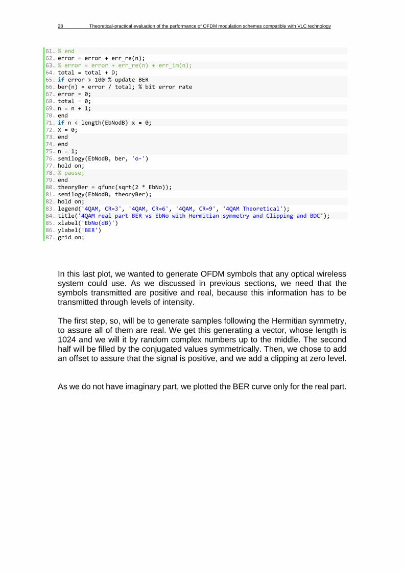
61. % end 62. error = error + err_re(n); 63. % error = error + err_re(n) + err_im(n); 64. total = total + D; 65. if error > 100 % update BER 66. ber(n) = error / total; % bit error rate 67. error = 0; 68. total = 0; 69. n = n + 1; 70. end 71. if n < length(EbNodB) x = 0; 72. X = 0; 73. end 74. end 75. n = 1; 76. semilogy(EbNodB, ber, 'o-') 77. hold on; 78. % pause; 79. end 80. theoryBer = qfunc(sqrt(2 * EbNo)); 81. semilogy(EbNodB, theoryBer); 82. hold on; 83. legend('4QAM, CR=3', '4QAM, CR=6', '4QAM, CR=9', '4QAM Theoretical'); 84. title('4QAM real part BER vs EbNo with Hermitian symmetry and Clipping and BDC'); 85. xlabel('EbNo(dB)') 86. ylabel('BER') 87. grid on;
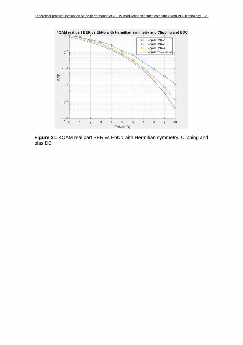
In this last plot, we wanted to generate OFDM symbols that any optical wireless system could use. As we discussed in previous sections, we need that the symbols transmitted are positive and real, because this information has to be transmitted through levels of intensity. The first step, so, will be to generate samples following the Hermitian symmetry, to assure all of them are real. We get this generating a vector, whose length is 1024 and we will it by random complex numbers up to the middle. The second half will be filled by the conjugated values symmetrically. Then, we chose to add an offset to assure that the signal is positive, and we add a clipping at zero level. As we do not have imaginary part, we plotted the BER curve only for the real part.
Theoretical-practical evaluation of the performance of OFDM modulation schemes compatible with VLC technology 29
Figure 21. 4QAM real part BER vs EbNo with Hermitian symmetry, Clipping and bias DC

30 Theoretical-practical evaluation of the performance of OFDM modulation schemes compatible with VLC technology
CHAPTER 3. DEMONSTRATION OF A VLC SYSTEM USING USRPs
3.1 Introduction
The previous MATLAB simulations gave me tools for implementing new code and understanding the basic concepts of a wireless system. In this new chapter, though, we are going to focus on the main work of this project: the real VLC demonstration. We want to implement a basic VLC system. We will divide the system by blocks: the USRP, the transmitter, the receiver, the LED and the photodetector. Because of time and knowledge limitations, the modulation used for the communication is going to be BPSK/OOK.
3.2 USRP connection and environment
3.2.1 Introduction to USRP
The Universal Radio Peripheral (USRP) enables designing and implementing powerful and flexible software radio systems. Thanks to a broad selection of daughter boards, it can cover a wide range of frequencies. The powerful combination of flexible hardware, open-source software and a community of experienced users makes it the ideal platform for our software radio development. In our system, all the wave-form specific processing is done on the host CPU (tasks such as modulation and demodulation), and the high-speed general-purpose operations (such as digital up/down conversion, decimation and interpolation) are done on the FPGA, in our case, the USRP (see [14]).
Figure 22. Main diagram of the System
Theoretical-practical evaluation of the performance of OFDM modulation schemes compatible with VLC technology 31
In the lab there are two different daughterboards. Each one has a different hardware (see [15]). In the Annex it is attached the procedure for the configuration and installation of the environment.
3.2.2 USRP Connection
The material needed will be:
- 2 PCs
- 2 USRPs
- 4 SMA wires
- 2 power supplies
- 2 ethernet LANs
- Oscilloscope and 2 oscilloscope probes
- External clock
- 2 ethernet interface cards
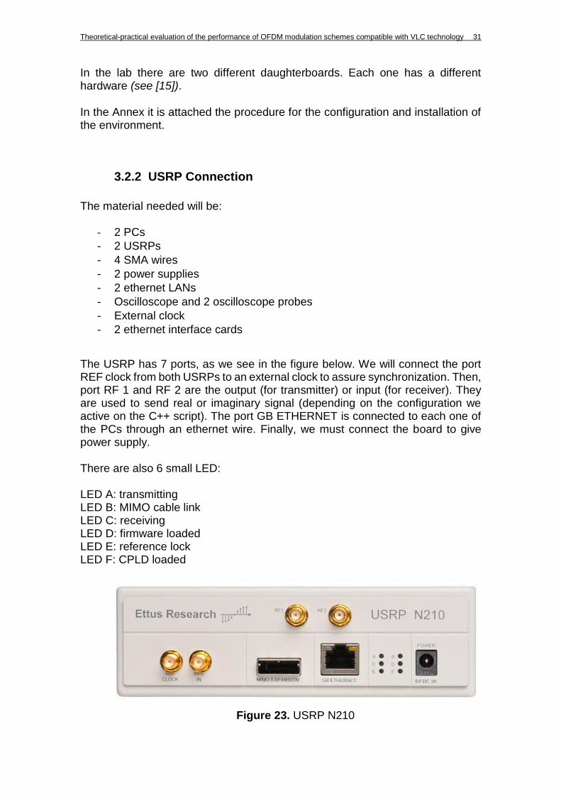
The USRP has 7 ports, as we see in the figure below. We will connect the port REF clock from both USRPs to an external clock to assure synchronization. Then, port RF 1 and RF 2 are the output (for transmitter) or input (for receiver). They are used to send real or imaginary signal (depending on the configuration we active on the C++ script). The port GB ETHERNET is connected to each one of the PCs through an ethernet wire. Finally, we must connect the board to give power supply. There are also 6 small LED: LED A: transmitting LED B: MIMO cable link LED C: receiving LED D: firmware loaded LED E: reference lock LED F: CPLD loaded Figure 23. USRP N210

32 Theoretical-practical evaluation of the performance of OFDM modulation schemes compatible with VLC technology
On a first try, we are not going to connect the LED and photodetector between the output of the transmitter USRP and the input of the receiver USRP. Conversely, we are going to substitute it by a wire, that will insert some attenuation to the system.
Figure 24. USRP transmitter (below) and USRP receiver (on the top)
Figure 25. Work environment

Theoretical-practical evaluation of the performance of OFDM modulation schemes compatible with VLC technology 33
3.3 Transmitter software implementation
In this section, it will be described how the transmitter software was implemented in order to set the parameters, load a file with random BPSK symbols, add artificial noise, add a preamble to ease the frame detection, include a matched filter (raised-cosine), adapt the samples to the range required by the LED and send them. The complete script is included at the end of the section (see [16]).
Figure 26. Software flow chart
3.3.1 Variables to be set
It is extremely important to set the same parameters at the transmitter and the receiver. The variables that need to be set are:
- IP address: 192.168.10.2
- The mode in which the ports (RF1, RF2) will work: A:AB. It means that
RF1 will send the real part and RF2, the imaginary part.
- The reference clock: external
- Transmission rate: 2e5.
3.3.2 Loading MATLAB file with BPSK symbols
We take advantage from the scripts we implemented at the beginning to write another script that generates random symbols and keeps them in a file called “initre.txt”. This file is loaded by the C++ script, reads each line and keeps it in a vector called readbuff [ ] from position 50 until the end (position 1000). This is because the first 50 positions of this vector are reserved for the preamble.

34 Theoretical-practical evaluation of the performance of OFDM modulation schemes compatible with VLC technology
1. clc; 2. clear all; 3. close all; % input value 4. N = 950 5. re4qam = [1 - 1]; 6. s = randsrc(1, N, re4qam); 7. inre = fopen('initre.txt', 'wt+'); 8. fprintf(inre, format, real(s)); 9. fclose(inre); 10. end
3.3.3 Adding noise
Before adding the LED and the photodetector, the aim is to test the system adding artificial noise with the program. To estimate the BER, it will be necessary to vary, manually, the EbdB, a value between 0 (very low SNR) and 10 (very high). Each time a BER value is calculated the process will be repeated after varying the EbNo. Again, the script is working by small blocks, in this case, short frames. The receiver will be receiving frames while the error counter is under 50. If it arrives to 50, the execution will stop, and it will be obtained the BER value. That is why the transmitter must send frames nonstop. To add the noise here, in the transmitter, each sample is contaminated by a gaussian noise. When we connect the LED and the photodetector, this function will be removed.
3.3.4 Preamble
The first 50 samples of the vector realbuff [ ] are reserved, as it was said before. The vector is going to be filled with 0 the first 3 positions and the last 3 zeros. For the rest, 1s and -1 will be alternated. The preamble is important to detect where the frame starts and be able to do the comparison between the information received and the original information. The preamble is not contaminated by noise to simplify the detection. Obviously, in a real channel, both preamble and information would be contaminated by the same amount of noise.
Figure 27. Random BPSK symbols (initre.txt)
Theoretical-practical evaluation of the performance of OFDM modulation schemes compatible with VLC technology 35
In this table, the filling of the preamble is shown:
3.3.5 Matched filter and oversampling
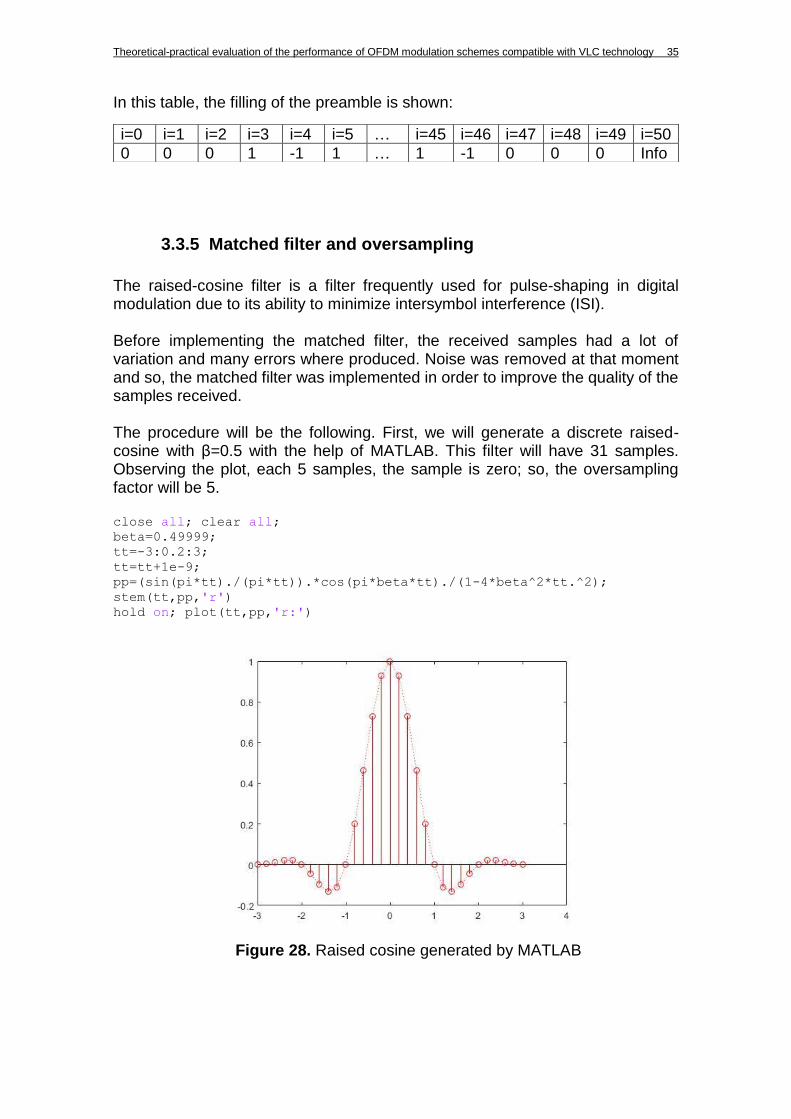
The raised-cosine filter is a filter frequently used for pulse-shaping in digital modulation due to its ability to minimize intersymbol interference (ISI). Before implementing the matched filter, the received samples had a lot of variation and many errors where produced. Noise was removed at that moment and so, the matched filter was implemented in order to improve the quality of the samples received. The procedure will be the following. First, we will generate a discrete raised-cosine with β=0.5 with the help of MATLAB. This filter will have 31 samples. Observing the plot, each 5 samples, the sample is zero; so, the oversampling factor will be 5. close all; clear all; beta=0.49999; tt=-3:0.2:3; tt=tt+1e-9; pp=(sin(pi*tt)./(pi*tt)).*cos(pi*beta*tt)./(1-4*beta^2*tt.^2); stem(tt,pp,'r') hold on; plot(tt,pp,'r:')
i=0 i=1 i=2 i=3 i=4 i=5 … i=45 i=46 i=47 i=48 i=49 i=50
0 0 0 1 -1 1 … 1 -1 0 0 0 Info
Figure 28. Raised cosine generated by MATLAB

36 Theoretical-practical evaluation of the performance of OFDM modulation schemes compatible with VLC technology
These are the coefficients of the raised-cosine filter generated by MATLAB:
txpulse[0] = 0;
txpulse[1] = 0.030;
txpulse[2] = 0.0119;
txpulse[3] = 0.0214;
txpulse[4] = 0.0211;
txpulse[5] = 0;
txpulse[6] = -0.0441;
txpulse[7] = -0.0981;
txpulse[8] = -0.1324;
txpulse[9] = -0.1095;
txpulse[10] = 0;
txpulse[11] = 0.2008;
txpulse[12] = 0.4634;
txpulse[13] = 0.7289;
txpulse[14] = 0.9268;
txpulse[15] = 1;
txpulse[30] = 0;
txpulse[29] = 0.030;
txpulse[28] = 0.0119;
txpulse[27] = 0.0214;
txpulse[26] = 0.0211;
txpulse[25] = 0;
txpulse[24] = -0.0441;
txpulse[23] = -0.0981;
txpulse[22] = -0.1324;
txpulse[21] = -0.1095;
txpulse[20] = 0;
txpulse[19] = 0.2008;
txpulse[18] = 0.4634;
txpulse[17] = 0.7289;
txpulse[16] = 0.9268;
The samples obtained after the noise addition are going to be convolved by this matched filter. As all the samples convolved by the matched filter will be summed, the coefficients obtained will be a sum of coefficients of the match filter and the original samples, except for the multiples of 5, which value will be exactly the value of the original sample. At the output of the convolution with the matched filter, the samples will be kept in the vector overbuff [ ], which length is 5030.
3.3.6 Adapting the samples to the LED range
At this point, the samples are bipolar. As it was studied before, for a wireless optical communication, it is needed to have positive values so that they can be modulated by the intensity of the light. In addition, not only they have to be positive, but they must also belong to the range stipulated by the LED specifications. As it is shown in the plot, the LED works in a linear way from 540 mV to 580 mV approximately.
0
5000
10000
15000
20000
25000
30000
35000
500 520 540 560 580 600 620 640
LUX
Vin (mV)
Vin - Luminosity
Figure 29. Operation region of the LED

Theoretical-practical evaluation of the performance of OFDM modulation schemes compatible with VLC technology 37
To accomplish with the requirements, the signal will be adapted to this range by dividing it by 20 and summing an offset of 0.56.
3.3.7 Sending the samples
The vector overbuff is ready to be transmitted to the USRP. We want the transmitter to work nonstop. For this, we implemented a way to fill the overbuff vector with new noise each time the vector is transmitted. With this characteristic, the BER obtained at the end of the chain will be more realistic. We kept in a file the vector overbuff to show its aspect and demonstrate that all the specifications mentioned before are implemented. 0.56 0.5615 0.560595 0.56107 0.561055 0.56 0.556295 0.5545 0.55231 0.55347 0.56 0.573745 0.58867
0.604135 0.61287 0.61 0.592595 0.567775 0.539035 0.51717 0.51 0.52193 0.545605 0.57606 0.600625 0.61
0.599125 0.575465 0.544535 0.520875 0.51 0.520875 0.544535 0.575465 0.599125 0.61 0.599125
These 37 values correspond to the first positions of the overbuff [ ] vector. The values in bold are exactly each one of the samples without mixing with other samples and the coefficients of the matched filter. As it is observed, the value 0.56 corresponds to the value zero (remember that the preamble starts with 3 zeros); the value 0.61 corresponds to a 1; and the value 0.51 corresponds to a -1.
3.3.8 Complete script
#include <uhd/utils/thread_priority.hpp>
#include <uhd/utils/safe_main.hpp>
#include <uhd/usrp/multi_usrp.hpp>
#include <uhd/exception.hpp>
#include <uhd/types/tune_request.hpp>
#include <boost/program_options.hpp>
#include <boost/format.hpp>
#include <boost/thread.hpp>

38 Theoretical-practical evaluation of the performance of OFDM modulation schemes compatible with VLC technology
#include <uhd/stream.hpp>
#include <iostream>
#include <string>
#include <fstream>
#include <complex>
#include <vector>
#include <algorithm>
#include <random>
using namespace std;
int UHD_SAFE_MAIN(int argc, char *argv[]) {
uhd::set_thread_priority_safe();
std::string device_args("addr=192.168.10.2");
std::string subdevtx("A:AB"); //IQ channel A=I B=Q AB=IQ BA=QI (A=RF1
B=RF2)
std::string ref("external");
//variables to be set
double rate(2e5);
int line_count = 50;
double SAMPLE = 1000;
string FID = "initre.txt";
//create a usrp device
uhd::usrp::multi_usrp::sptr usrp = uhd::usrp::multi_usrp::make(device_args);
//for synchronization
usrp->set_clock_source(ref);
//set PPS
//usrp->set_time_source(ref);
//usrp->set_tx_subdev_spec(subdevtx);
usrp->set_tx_rate(rate);
//create a transmit streamer
uhd::stream_args_t stream_args("fc32", "sc16");
uhd::tx_streamer::sptr tx_stream = usrp->get_tx_stream(stream_args);
uhd::tx_metadata_t md;
//read the both real and imag signal text file
//allocate buffer with data to send
std::default_random_engine generator;
std::normal_distribution<double> distribution(0.0, 1.0);
int count = 0;
string line;
string line1;
vector < complex < float>> readbuff(SAMPLE), txpulse(31);
txpulse[0] = 0;
txpulse[1] = 0.030;
txpulse[2] = 0.0119;
txpulse[3] = 0.0214;
txpulse[4] = 0.0211;
txpulse[5] = 0;
txpulse[6] = -0.0441;
txpulse[7] = -0.0981;
txpulse[8] = -0.1324;
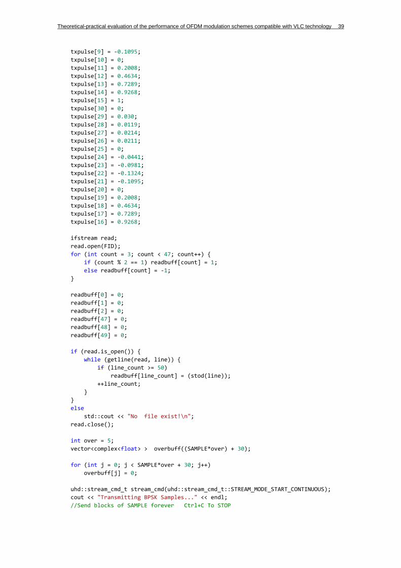
Theoretical-practical evaluation of the performance of OFDM modulation schemes compatible with VLC technology 39
txpulse[9] = -0.1095;
txpulse[10] = 0;
txpulse[11] = 0.2008;
txpulse[12] = 0.4634;
txpulse[13] = 0.7289;
txpulse[14] = 0.9268;
txpulse[15] = 1;
txpulse[30] = 0;
txpulse[29] = 0.030;
txpulse[28] = 0.0119;
txpulse[27] = 0.0214;
txpulse[26] = 0.0211;
txpulse[25] = 0;
txpulse[24] = -0.0441;
txpulse[23] = -0.0981;
txpulse[22] = -0.1324;
txpulse[21] = -0.1095;
txpulse[20] = 0;
txpulse[19] = 0.2008;
txpulse[18] = 0.4634;
txpulse[17] = 0.7289;
txpulse[16] = 0.9268;
ifstream read;
read.open(FID);
for (int count = 3; count < 47; count++) {
if (count % 2 == 1) readbuff[count] = 1;
else readbuff[count] = -1;
}
readbuff[0] = 0;
readbuff[1] = 0;
readbuff[2] = 0;
readbuff[47] = 0;
readbuff[48] = 0;
readbuff[49] = 0;
if (read.is_open()) {
while (getline(read, line)) {
if (line_count >= 50)
readbuff[line_count] = (stod(line));
++line_count;
}
}
else
std::cout << "No file exist!\n";
read.close();
int over = 5;
vector<complex<float> > overbuff((SAMPLE*over) + 30);
for (int j = 0; j < SAMPLE*over + 30; j++)
overbuff[j] = 0;
uhd::stream_cmd_t stream_cmd(uhd::stream_cmd_t::STREAM_MODE_START_CONTINUOUS);
cout << "Transmitting BPSK Samples..." << endl;
//Send blocks of SAMPLE forever Ctrl+C To STOP

40 Theoretical-practical evaluation of the performance of OFDM modulation schemes compatible with VLC technology
while (1) {
double w;
int EbdB = 50; //Entre 0 y 10
double EbNo = pow(10, EbdB / 10);
for (int j = 3; j < SAMPLE; j++) {
for (int jj = 0; jj < 31; jj++)
overbuff[5 * j + jj - 15] = overbuff[5 * j + jj - 15] + readbuff[j] *
txpulse[jj];
}
for (int j = 0; j < SAMPLE*over; j++) {
overbuff[j] = real(overbuff[j]) / 20 + 0.56;
}
//Guardar overbuff en fichero
/*ofstream myfile;
myfile.open("transmitted.txt");
for (int k = 0; k < SAMPLE*over; k++)
myfile << real(overbuff[k]) << endl;
cout << "The files are written!" << endl;
system("pause");*/
size_t tx_num = tx_stream->send(&overbuff.front(), SAMPLE*over, md, 0.05);
/*for (int g = 0; g < 300; g++)
cout <<g<<": "<< overbuff[g] << endl;
system("pause");*/
}
system("pause");
return EXIT_SUCCESS;
}
3.4 Receiver software implementation
The aim of the receiver software is to receive the frames, detect the preamble and keep the information of each of the frames to check how many errors were committed by comparing them with the original information. Remember that the initial aim of this system is not to send information, but to evaluate its performance. That is why the information file is in both transmitter and receiver. First, we have to set the same values for the parameters as we set on the transmitter. If it is not done like this, many errors will be produced, and the communication will not be possible. It is important to emphasize the command sleep_for. If we want that the vector of the receiver fills properly, we must wait a prudential time for the buffer to receive all the samples. So, before starting receiving, this command is implemented.

Theoretical-practical evaluation of the performance of OFDM modulation schemes compatible with VLC technology 41
3.4.1 Defined vectors
It is important to mention and describe each of the vectors used in this script to understand the general process. On the script there may be other vector declared, but finally, most of them were not used, they were created for other use and finally they were not taken advantage of. recv [10060]: When we start executing the receiver script, the first 10060 samples received are kept in this vector. The length of the vector has a reason: it is desired that in this vector can fit two entire frames, because from this vector we are going to detect the preamble and save the data in another vector.
N-250+4750+250+4750+N=10000 There are 60 more positions needed for compensating the matched filter. pream [50]: This vector is initialized. The first 3 positions and the last 3 positions are zero and the rest are alternated 1 and -1. His function will be to detect the preamble.
overwindow [250]: This vector is filled from the vector recv[10060]. Here it will be applied the undone of the matched filter and the result (5 times shorter) will be kept in the vector window [50].
Preamble Frame 1 Length = N- 250
Information Frame 1 950*5=4750
Preamble Frame 2 Length = 250
Information Frame 2 950*5=4750
Remaining space (N)
i=0 i=1 i=2 i=3 i=4 i=5 … i=45 i=46 i=47 i=48 i=49
0 0 0 1 -1 1 … 1 -1 0 0 0
Figure 30. Receiver flow chart

42 Theoretical-practical evaluation of the performance of OFDM modulation schemes compatible with VLC technology
window [50]: It will compare his content with the content of pream [50]. If they are equal, it means that the preamble has been found. tramarec [950]: Here the information without the preamble will be kept. matchedfilter [31]: This vector contains the coefficients of the matched filter and will be used to undo the process and obtain the vector window [50].
3.4.2 Preamble detection and matched filter
The correctly detection of the preamble is fundamental to carry out the process: without it, it is impossible to know where the frame starts. As it was said in the previous section, the first samples are kept in the vector recv [10060]. The vector overwindow [250] keeps the first 250 samples and the process of undoing the match filter in done from this vector. Again, we have to convolute this vector with the matchedfilter [31] to obtain the vector window [50]. The vector window [50] is now compared with the vector pream [50]. If they are equal, the preamble is fond. If not, the vector window [50] is moved a position and repeats the process. If any preamble was found on the first 5250 movements, it means that an error occurred, and the process has to start again. Once the preamble is found, the information is saved on the vector tramarec [950] and we are ready to compare it with the original information.
3.4.3 Demodulation
Because we are working on a very simple modulation, the demodulation does not have any complexity. If the line attached here we see that, when the values of tramarec [h] are positive, they become 1; while if they are negative, the become -1.
tramarec[h] = -1 * (real(tramarec[h]) < 0) + 1 * (real(tramarec[h]) >= 0);
3.4.4 Error counter
At this point, the original MATLAB file “initre.txt” must be loaded. We will compare each one of the positions of tramarec [950] with each of the lines of the file with a simple multiplication. If its result is negative, an error will be counted.
Theoretical-practical evaluation of the performance of OFDM modulation schemes compatible with VLC technology 43
3.4.5 BER obtaining
As it was explained at previous sections, the receiver repeats the whole process until 50 errors are found. If the noise is very high, it is probably that only the processing of one frame is needed. But, if the signal has a very high quality, it will be needed to process many frames, and consequently, repeat parts of the process. The detection of the preamble must be done each time a frame has to be processed. An upgrade of the script could be done to avoid detecting the preamble all the time, but it was a very complex implementation.
3.4.6 Complete script
//Ctrl+F5 to execute the program
#include <uhd/utils/thread_priority.hpp>
#include <uhd/utils/safe_main.hpp>
#include <uhd/usrp/multi_usrp.hpp>
#include <uhd/exception.hpp>
#include <uhd/types/tune_request.hpp>
#include <boost/program_options.hpp>
#include <boost/format.hpp>
#include <boost/thread.hpp>
#include <complex>
#include <uhd/stream.hpp>
#include <iostream>
#include <fstream>
#include <vector>
#include <algorithm>
#include <chrono>
#include <thread>
using namespace std;
int UHD_SAFE_MAIN(int argc, char *argv[]) {
uhd::set_thread_priority_safe();
std::string device_args("addr=192.168.10.2");
std::string subdevrx("A:AB"); //IQ channel A=I B=Q AB=IQ BA=QI (A=RF1
B=RF2)
std::string ref("external");
using namespace std::this_thread; // sleep_for, sleep_until
using namespace std::chrono_literals; // ns, us, ms, s, h, etc.
using std::chrono::system_clock;
//variables to be set
double rate(2e5);
double freq(0);
int over = 5;
int prefixno = 50;
double SAMPLE = 50;
double gain = 0; //set 0 to 6
44 Theoretical-practical evaluation of the performance of OFDM modulation schemes compatible with VLC technology
uhd::usrp::multi_usrp::sptr usrp = uhd::usrp::multi_usrp::make(device_args);
//create a usrp
device
usrp->set_clock_source(ref); //set the clock
usrp->set_rx_rate(rate);
usrp->set_rx_gain(gain);
usrp->set_rx_freq(freq);
std::cout << "rx_rate= " << usrp->get_rx_rate() << endl;
std::cout << "rx_gain= " << usrp->get_rx_gain() << endl;
std::cout << "rx_freq= " << usrp->get_rx_freq() << endl;
std::cout << "Sample number= " << SAMPLE / over << endl;
//create a receive streamer
uhd::stream_args_t stream_args("fc32", "sc16");
/*std::vector<size_t> channel_nums; stream_args.channels = channel_nums;*/
uhd::rx_streamer::sptr rx_stream = usrp->get_rx_stream(stream_args);
uhd::rx_metadata_t mdr;
uhd::rx_metadata_t md;
//Start streaming
uhd::stream_cmd_t stream_cmd(uhd::stream_cmd_t::STREAM_MODE_NUM_SAMPS_AND_DONE);
rx_stream->issue_stream_cmd(stream_cmd);
//receive in a text file
ofstream myfile;
myfile.open("recvre.txt");
ofstream myfile2;
myfile.open("overrecvre.txt");
//allocate buffer for receiver
vector<complex<double> > buffrx(SAMPLE);
// for preamble
int pre = prefixno * over;
int count = 0;
int i = 1;
int cont_errores = 0;
vector<complex<float> > precheck(10);
vector<complex<float> > preamble(prefixno);
vector<complex<double> > oversamp(pre);
vector<complex<float> > recv(10060), pream(50), overwindow(250), window(50),
tramarec(950), matchedfilter(31);
matchedfilter[0] = 0;
matchedfilter[1] = 0.030;
matchedfilter[2] = 0.0119;
matchedfilter[3] = 0.0214;
matchedfilter[4] = 0.0211;
matchedfilter[5] = 0;
matchedfilter[6] = -0.0441;
matchedfilter[7] = -0.0981;
matchedfilter[8] = -0.1324;
matchedfilter[9] = -0.1095;
matchedfilter[10] = 0;
matchedfilter[11] = 0.2008;
matchedfilter[12] = 0.4634;
matchedfilter[13] = 0.7289;
matchedfilter[14] = 0.9268;
matchedfilter[15] = 1;
matchedfilter[0] = 0;
matchedfilter[30] = 0.030;
Theoretical-practical evaluation of the performance of OFDM modulation schemes compatible with VLC technology 45
matchedfilter[29] = 0.0119;
matchedfilter[28] = 0.0214;
matchedfilter[28] = 0.0211;
matchedfilter[26] = 0;
matchedfilter[25] = -0.0441;
matchedfilter[24] = -0.0981;
matchedfilter[23] = -0.1324;
matchedfilter[22] = -0.1095;
matchedfilter[21] = 0;
matchedfilter[20] = 0.2008;
matchedfilter[19] = 0.4634;
matchedfilter[18] = 0.7289;
matchedfilter[17] = 0.9268;
matchedfilter[16] = 1;
for (int h = 0; h < 10060; h++)
recv[h] = -5;
sleep_for(0.0525s);
rx_stream->recv(&recv.front(), 10060, md, 0.001);
//Cargar fichero de texto con el que compararemos
string FIF = "initre.txt";
ifstream read;
read.open(FIF);
string line;
int k = 0;
std::vector<double> initre(950);
if (read.is_open())
while (getline(read, line))
{
initre[k] = (stod(line));
++k;
}
//**************DETECTAR PREAMBULO************
cout << "Receiving BPSK Samples..." << endl;
//Receive SAMPLE forever Ctrl+C To STOP
for (int d = 0; d < 44; d++) {
if (d % 2 == 1) pream[d] = -1;
else pream[d] = 1;
}
for (int d = 0; d < 250; d++)
overwindow[d] = (real(recv[d]));
//******************MATCHED FILTER***************
for (int d=3; d<47; d++){
window[d] = 0;
for (int dd = 0; dd < 31; dd++)
window[d] = window[d] + real(overwindow[5 * d + dd]) *
real(matchedfilter[dd]);
//std::cout << "window: " << d << " " << window[d] << endl;
window[d] = -1 * (real(window[d]) < 0) + 1 * (real(window[d])>= 0);
//std::cout << "window: " << d << " " << window[d] << endl;
}

46 Theoretical-practical evaluation of the performance of OFDM modulation schemes compatible with VLC technology
int flag = 1, kk = 0;
while (flag){
kk = kk + 1;
int counter = 0;
for (int dd = 3; dd < 47; dd++)
if (abs(real(pream[dd-3]) - real(window[dd])) < 0.01)counter++;
if (counter < 44)
{
for (int f = 0; f < 249; f++)
overwindow[f] = overwindow[f + 1];
overwindow[249] = real(recv[249 + kk]);
for (int d = 3; d < 47; d++) {
window[d] = 0;
for (int dd = 0; dd < 31; dd++)
window[d] = window[d] + real(overwindow[5 * d + dd]) *
real(matchedfilter[dd]);
window[d] = -1 * (real(window[d]) < 0) + 1 * (real(window[d]) >= 0);
}
}
else
{
std::cout << "llego" << endl;
for (int h = 0; h < 950; h++) {
tramarec[h] = 0;
for (int dd = 0; dd < 31; dd++)
tramarec[h] = tramarec[h] + real(recv[249 + kk + 5*h + 15 +2 -15
+ dd]) * real(matchedfilter[dd]);
tramarec[h] = -1 * (real(tramarec[h]) < 0) + 1 * (real(tramarec[h])
>= 0);
if (initre[h] * (real(tramarec[h])) < 0)
cont_errores++;
}
cout << cont_errores << "........errores" << endl;
//Guardar recv en fichero
ofstream myfile, mufile2;
myfile.open("received.txt");
myfile2.open("sym_recv.txt");
for (int k = kk; k < 1000*over+kk; k++)
myfile<<recv[k] <<endl;
for (int k = 0; k < 950; k++)
myfile2 << tramarec[k] << endl;
cout << "The files are written!" << endl;
system("pause");
}
}
system("pause");
return EXIT_SUCCESS;
}

Theoretical-practical evaluation of the performance of OFDM modulation schemes compatible with VLC technology 47
3.5 LED Driver Circuit and Photodetector
In this section, the chosen LED and photodetector will be briefly described as well as the LED driver circuit. At the circuit, there is a voltage buffer amplifier with unity gain. It is used to adapt the USRP signal and isolate the USRP from other parts of the circuit to prevent damaging it.
The second device is an operational amplifier to amplify the USRP signal since its level is too low for the next stage to work without amplification. For power supplying, there is a power amplifier. It should be polarized to work independently when the output signal from the second device is not connected to the input. When the signal is connected, the power amplifier will vary the voltage across the LED to change its light intensity.
Figure 31. LED Driver circuit
Figure 32. LED Driver Circuit scheme

48 Theoretical-practical evaluation of the performance of OFDM modulation schemes compatible with VLC technology
This LED uses a MOSFET as the power amplifier while that MOSFET is designed for on-off application. It means that its response is non-linear. The range between the maximum and minimum of the input voltage is very narrow, as we saw on the transmitter section. It acts like a switch and the threshold is at 500 mV. When the voltage is smaller than the threshold, it will not turn on. However, when it is 600 mV, it will be its maximum voltage at the output. There is only 100mV for the range of input voltage to perform transmission, which mean that a small variation will affect the quality of transmission greatly. Moreover, there is a distortion at the output. This problem is due to the non-linear characteristic of LED. When we have a sinusoidal input voltage, distortion occurs at the output of the voltage across the LED.
3.6 Complete system and results
At this point of the project, we are going to substitute the wire that used to connect both USRP by the LED and the photodetector. It will not be possible to evaluate the BER for different EbNo because it is not easy to estimate the total noise of the channel. So, the mounting has consisted in placing the LED and the photodetector, one in front of the other, at approximately 25 cm of distance, looking for the optimal position so there was the minimum noise and the detector could do its best. It is important to remark that, due to the simplicity of the preamble designed, if the EbNo is too high, any kind of communication would be possible, because the preamble could not be detected, and we could not estimate any BER.
Figure 33. Photodetector

Theoretical-practical evaluation of the performance of OFDM modulation schemes compatible with VLC technology 49
Fortunately, the system worked properly when the LED and the photodetector had a perfect line of sight, getting very good results. We tested the system many times and in most of the cases the errors counted where 0. In the figures below there are some screen captures of one of that tests, where we got 0 errors. The file “initre.txt” remains to the original information and the file “sym_recv-1.txt” remains to the demodulated symbols at the receiver. At first sight, we can observe that the symbols received are exactly the same.
Figure 34. Complete system in an optimal position
Figure 35. Comparison between the original file and the symbols received
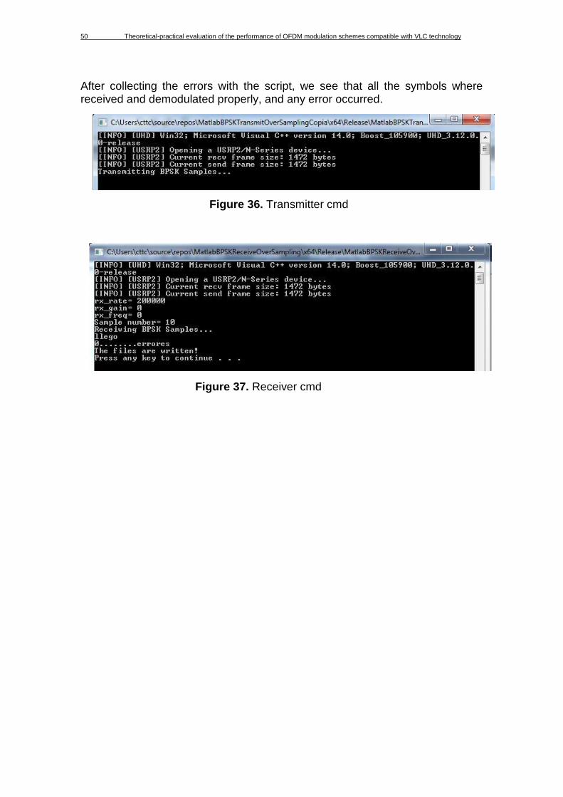
50 Theoretical-practical evaluation of the performance of OFDM modulation schemes compatible with VLC technology
After collecting the errors with the script, we see that all the symbols where received and demodulated properly, and any error occurred.
Figure 36. Transmitter cmd
Figure 37. Receiver cmd

Theoretical-practical evaluation of the performance of OFDM modulation schemes compatible with VLC technology 51
CONCLUSIONS Along the project VLC technology was introduced, as well as its main modulation schemes. OFDM was outstanding because of its advantages. Several MARLAB simulations were implemented in order to understand better the behavior of each one of them and know its performance, basing it on the BER result. Finally, a real VLC system was demonstrated using USRP daughterboards. The most important part was the development of the transmitter and receiver software, written in C++ and adapted for the correct USRP reading through UHD. The complete system, with the LED and the photodetector, was mounted and it worked perfectly. The final modulation scheme implemented was BPSK, due to its simplicity. The scheme was adapted to an OOK version: when 1s were sent, the intensity level was 0.61; and when -1s were sent, it was 0.51 (following the LED linear range, which was very narrow). It is obvious that with a more complex modulation, higher bit rates could be obtained, if the LED was closed to the photodetector, because the SNR would be high. The preamble detection was one of the weaknesses of the system. If the LED was too far from the photodetector or it didn’t have direct line of sight, the errors were very high, and they affected the preamble detection, so any bit could be processed. In an upgrade of the project, the mechanism of the preamble should be improved, as well as the work range of the LED by modifying the driver circuit or selecting another LED. It also could be a good idea to implement more complex modulations in the software, such as OFDM, as long as the lineal zone of the LED has widened. After this project, I realize of the problems that wireless communications must fight against. Many aspects were simplified due to lack of time and lack of knowledges. In most of wireless systems, we can find tools such as automatic gain control, to palliate the EbNo when the noise is very high; error correction or more sophisticated techniques for the synchronization of the frames. This project is a very good introduction to visible light communications. Also, it has many points to continue developing implementations and improving the system.
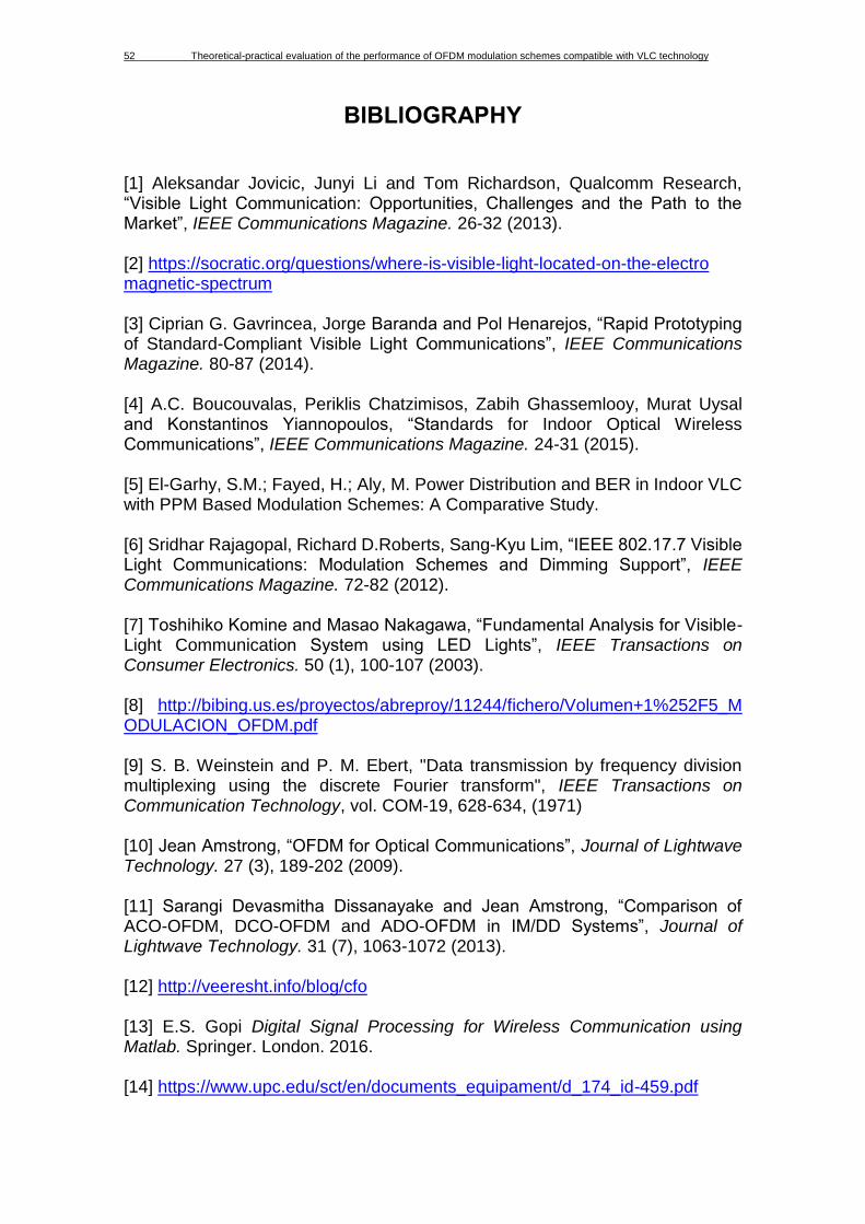
52 Theoretical-practical evaluation of the performance of OFDM modulation schemes compatible with VLC technology
BIBLIOGRAPHY [1] Aleksandar Jovicic, Junyi Li and Tom Richardson, Qualcomm Research, “Visible Light Communication: Opportunities, Challenges and the Path to the Market”, IEEE Communications Magazine. 26-32 (2013). [2] https://socratic.org/questions/where-is-visible-light-located-on-the-electro magnetic-spectrum [3] Ciprian G. Gavrincea, Jorge Baranda and Pol Henarejos, “Rapid Prototyping of Standard-Compliant Visible Light Communications”, IEEE Communications Magazine. 80-87 (2014). [4] A.C. Boucouvalas, Periklis Chatzimisos, Zabih Ghassemlooy, Murat Uysal and Konstantinos Yiannopoulos, “Standards for Indoor Optical Wireless Communications”, IEEE Communications Magazine. 24-31 (2015). [5] El-Garhy, S.M.; Fayed, H.; Aly, M. Power Distribution and BER in Indoor VLC with PPM Based Modulation Schemes: A Comparative Study. [6] Sridhar Rajagopal, Richard D.Roberts, Sang-Kyu Lim, “IEEE 802.17.7 Visible Light Communications: Modulation Schemes and Dimming Support”, IEEE Communications Magazine. 72-82 (2012). [7] Toshihiko Komine and Masao Nakagawa, “Fundamental Analysis for Visible-Light Communication System using LED Lights”, IEEE Transactions on Consumer Electronics. 50 (1), 100-107 (2003). [8] http://bibing.us.es/proyectos/abreproy/11244/fichero/Volumen+1%252F5_M ODULACION_OFDM.pdf [9] S. B. Weinstein and P. M. Ebert, "Data transmission by frequency division multiplexing using the discrete Fourier transform", IEEE Transactions on Communication Technology, vol. COM-19, 628-634, (1971) [10] Jean Amstrong, “OFDM for Optical Communications”, Journal of Lightwave Technology. 27 (3), 189-202 (2009). [11] Sarangi Devasmitha Dissanayake and Jean Amstrong, “Comparison of ACO-OFDM, DCO-OFDM and ADO-OFDM in IM/DD Systems”, Journal of Lightwave Technology. 31 (7), 1063-1072 (2013). [12] http://veeresht.info/blog/cfo [13] E.S. Gopi Digital Signal Processing for Wireless Communication using Matlab. Springer. London. 2016. [14] https://www.upc.edu/sct/en/documents_equipament/d_174_id-459.pdf

Theoretical-practical evaluation of the performance of OFDM modulation schemes compatible with VLC technology 53
[15] http://www.ni.com/white-paper/53624/es/ [16] https://files.ettus.com/manual/index.html

54 Theoretical-practical evaluation of the performance of OFDM modulation schemes compatible with VLC technology
APPENDICES

Theoretical-practical evaluation of the performance of OFDM modulation schemes compatible with VLC technology 55
1.1 USRP Hardware Driver
For the Windows users, UHD software installers are provided by Ettus
Research which is a binary installation. Here is an example of using Visual
Studio to start using the UHD, the configuration is below.
1.1.1 Host Computer
Operative System: Windows 7/10
Development Environment: Microsoft Visual Studio Community 2017
1.1.2 1.1.2 Microsoft Visual Studio Development environment configuration
Install Microsoft Visual Studio Community 2017:
https://visualstudio.microsoft.com/downloads/
Choose the C++ Development Installation:
Figure 38. Available downloads
1.1.3 Install Boost boost_1_67_0_b1-msvc-14.1-64.exe for windows
64bits: https://sourceforge.net/projects/boost/files/boost-binaries/1.67.0_b1/

56 Theoretical-practical evaluation of the performance of OFDM modulation schemes compatible with VLC technology
1.1.4 Install the latest UHD
UHD installer: http://files.ettus.com/binaries/uhd/latest_release/
Figure 39. UHD installer
Figure 40. Choose 64 bits option
Figure 41. Choose: Do not add UHD to the system PATH

Theoretical-practical evaluation of the performance of OFDM modulation schemes compatible with VLC technology 57
Follow the default steps.
Figure 43. The file after installation
1.1.5 Setting Environment Variables
Add UHD bin path to the Environment Variables so command prompt can
identify the command of UHD. Find out the Advanced system settings in the
Control Panel System.
Figure 42. Default destination folder (can be changed)
Figure 44. Control panel -> System and Security->System

58 Theoretical-practical evaluation of the performance of OFDM modulation schemes compatible with VLC technology
Figure 45. Click Environment Variables
Figure 46. Edit the path
Figure 47. Add the path of UHD\bin. Click OK.

Theoretical-practical evaluation of the performance of OFDM modulation schemes compatible with VLC technology 59
1.2 Build the Project in VS2017
File→New→Project
Figure 48. Choose Empty Project.
Figure 49. Change to x64 (bits)
Figure 50. Add New Item

60 Theoretical-practical evaluation of the performance of OFDM modulation schemes compatible with VLC technology
Figure 51. Choose C++ File (.cpp)
Figure 52. Right click UHD_Test > Properties / View > Property Pages
Figure 53. Configuration: Release; Platform: Active(x64) /Active(Win32) for 32bits; C/C++ > General > Additional Include Directories
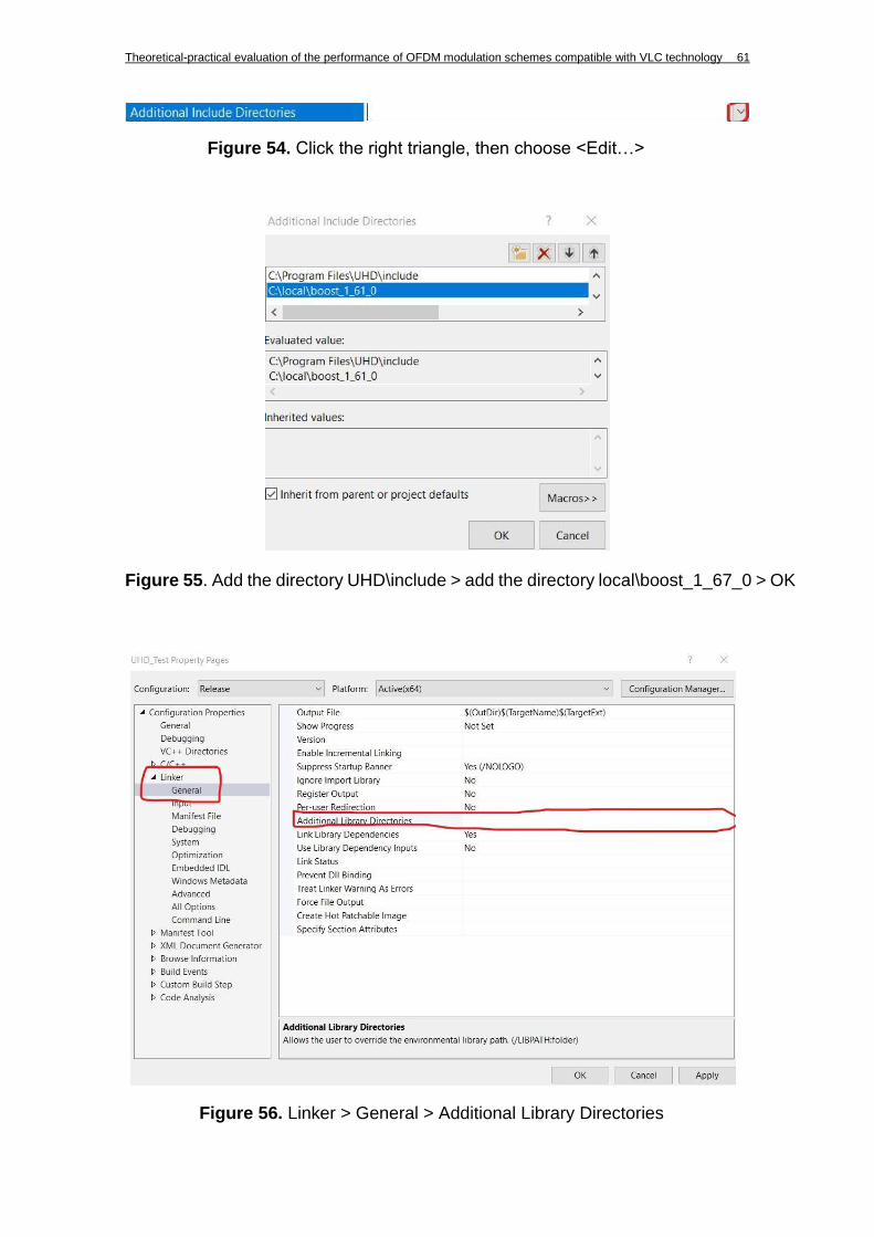
Theoretical-practical evaluation of the performance of OFDM modulation schemes compatible with VLC technology 61
Figure 54. Click the right triangle, then choose <Edit…>
Figure 55. Add the directory UHD\include > add the directory local\boost_1_67_0 > OK
Figure 56. Linker > General > Additional Library Directories

62 Theoretical-practical evaluation of the performance of OFDM modulation schemes compatible with VLC technology
Add the following code to the main.cpp for getting basic equipment connection information:
Figure 57. <edit…> > Add the directory UHD\lib > add the directory local\boost_1_67_0\lib64-msvc-14.1 > OK
Figure 58. Linker > Input > Additional Dependencies > Add uhd.lib; > OK
Figure 59. Change to Release

Theoretical-practical evaluation of the performance of OFDM modulation schemes compatible with VLC technology 63
1. //General Includes 2. #include < cmath > 3. #include < complex > 4. #include < csignal > 5. #include < fstream > 6. #include < iostream > 7. //UHD Includes 8. 9. #include < uhd / exception.hpp > 10. #include < uhd / types / tune_request.hpp > 11. #include < uhd / usrp / multi_usrp.hpp > 12. #include < uhd / utils / safe_main.hpp > 13. #include < uhd / utils / static.hpp > 14. #include < uhd / utils / thread_priority.hpp > 15. //Boost Includes 16. #include < boost / algorithm / string.hpp > 17. #include < boost / foreach.hpp > 18. #include < boost / format.hpp > 19. #include < boost / lexical_cast.hpp > 20. #include < boost / math / special_functions / round.hpp > 21. #include < boost / program_options.hpp > 22. #include < boost / thread / thread.hpp > 23. 24. int main(void) { // Look for connected USRPs 25. uhd::device_addr_t hint; 26. uhd::device_addrs_t device_addrs = uhd::device::find(hint); 27. // Exit if none were found 28. if (device_addrs.size() == 0) std::cerr << "No UHD Devices Found" << std::end
l; 29. //Display the USRPs Found 30. else 31. for (size_t i = 0; 1 < device_addrs.size(); i++) { 32. std::cout << "--------------------------------------------
" << std::endl; 33. std::cout << "--UHD Device" << i << std::endl; 34. std::cout << "--------------------------------------------
" << std::endl; 35. std::cout << device_addrs[i].to_pp_string() << std::endl << std::endl
; 36. } //Pause for the user 37. system("pause"); //Exit the program 38. return 0; 39. }
1.3 USRP Connection
1.3.1 Hardware
There are 2 USRP for this project. They are used as a transmitter and receiver separately.
Daughter board LFTX (for transmitting) LFRX (for receiving)
Version USRP N210
IP Address 192.168.10.2
Type usrp2

64 Theoretical-practical evaluation of the performance of OFDM modulation schemes compatible with VLC technology
1.3.2 Host computer IP Configuration
It can be any 192.168.10.X excepting the same IP as USRP. PC1 for transmitting IP address: 192.168.10.1 Subnet: 255.255.255.0 PC2 for receiving IP address:192.168.10.3 Subnet: 255.255.255.0
1.3.3 Command Checking
Open cmd.exe by typing cmd in start and type uhd_find_devices.
Now type uhd_usrp_probe.
Figure 60. cmd display when USRP is connected
Figure 61. This command can display the hardware of USRP. For example, knowing the daughterboard type whether it is LFTX/LFRX.

Theoretical-practical evaluation of the performance of OFDM modulation schemes compatible with VLC technology 65
1.3.4 Updating UHD Image Loader
Type uhd_image_loader --arg=”type=usrp2”
Figure 62. Updating the firmware of USRP when it is old