end-to-end learning of coherent probabilistic forecasts

End-to-End Learning of Coherent Probabilistic Forecasts forHierarchical Time Series

Syama Sundar Rangapuram 1 Lucien D. Werner 2 3 Konstantinos Benidis 1 Pedro Mercado 1 Jan Gasthaus 1

Tim Januschowski 1

Abstract

This paper presents a novel approach to forecast-ing of hierarchical time series that produces co-herent, probabilistic forecasts without requiringany explicit post-processing step. Unlike the state-of-the-art, the proposed method simultaneouslylearns from all time series in the hierarchy andincorporates the reconciliation step as part of asingle trainable model. This is achieved by apply-ing the reparameterization trick and utilizing theobservation that reconciliation can be cast as anoptimization problem with a closed-form solution.These model features make end-to-end learning ofhierarchical forecasts possible, while accomplish-ing the challenging task of generating forecaststhat are both probabilistic and coherent. Impor-tantly, our approach also accommodates generalaggregation constraints including grouped, tempo-ral, and cross-temporal hierarchies. An extensiveempirical evaluation on real-world hierarchicaldatasets demonstrates the advantages of the pro-posed approach over the state-of-the-art.

1. IntroductionIn many practically important applications, multivariatetime series have a natural hierarchical structure, where timeseries at upper levels of hierarchy are aggregates of thoseat lower levels (Petropoulos et al., 2020). Prominent exam-ples include retail sales, where sales are tracked at product,store, state and country levels (Seeger et al., 2016; 2017),and electricity forecasting, where consumption/productionquantities are desired at the individual, grid, and regionallevels (Taieb et al., 2020; Jeon et al., 2019). Although seriesat the bottom of the hierarchy are typically sparse, noisy

1AWS AI Labs, Germany. 2Department of Computing & Math-ematical Sciences, California Institute of Technology, Pasadena,California, USA. 3Work done while at Amazon. Correspondenceto: Syama S. Rangapuram <[email protected]>.

Proceedings of the 38 th International Conference on MachineLearning, PMLR 139, 2021. Copyright 2021 by the author(s).

and devoid of the high level patterns that are apparent inaggregate (Ben Taieb et al., 2017), forecasts have valueat all levels: bottom-level forecasts may be of more inter-est for automated decision making on operational horizonswhereas forecasts at the top level enable strategic decisionmaking (Januschowski & Kolassa, 2019). However, generat-ing forecasts independently for time series at each level doesnot guarantee that the forecasts are coherent, i.e., forecastsof aggregated time series are the sum of forecasts of thecorresponding disaggregated time series.

Thus, the main challenge of forecasting hierarchical timeseries is to exploit the information available across all levelsof a given hierarchy while producing coherent forecasts.Prior work in hierarchical forecasting follows a two-stageapproach: base forecasts are first obtained independentlyfor each time series in the hierarchy and are then combinedand revised in a post-processing step to ensure coherence.Two main issues arise with such a two-stage procedure: (i)the model parameters for each time series are learned inde-pendently, thereby discarding information, and (ii) the baseforecasts are revised without any regard to the learned modelparameters. Another fundamental limitation of most exist-ing methods is that they can only produce point (rather thanprobabilistic) forecasts. Probabilistic forecasts are requiredin practice for better decision making and risk manage-ment (Berrocal et al., 2010). The notable exception is (BenTaieb et al., 2017), although it is still a two-step procedure.

In this work, we present a novel approach to probabilisticforecasting of hierarchical time series that incorporates bothlearning and reconciliation into a single end-to-end model.Model parameters are learned simultaneously from all timeseries in the hierarchy. The probabilistic forecasts from themodel are guaranteed to be coherent without requiring anypost-processing step. The key insights behind the proposedmethod are the differentiability of the sampling operation,thanks to the reparametrization trick (Kingma & Welling,2013), and the implementation of the reconciliation step onsamples as a convex optimization problem. This allows oneto combine typically independent components (generationof base forecasts, sampling and reconciliation) into a singletrainable model.

End-to-End Learning of Coherent Probabilistic Forecasts for Hierarchical Time Series

y

y1

b1 b2

y2

b3 b4 b5

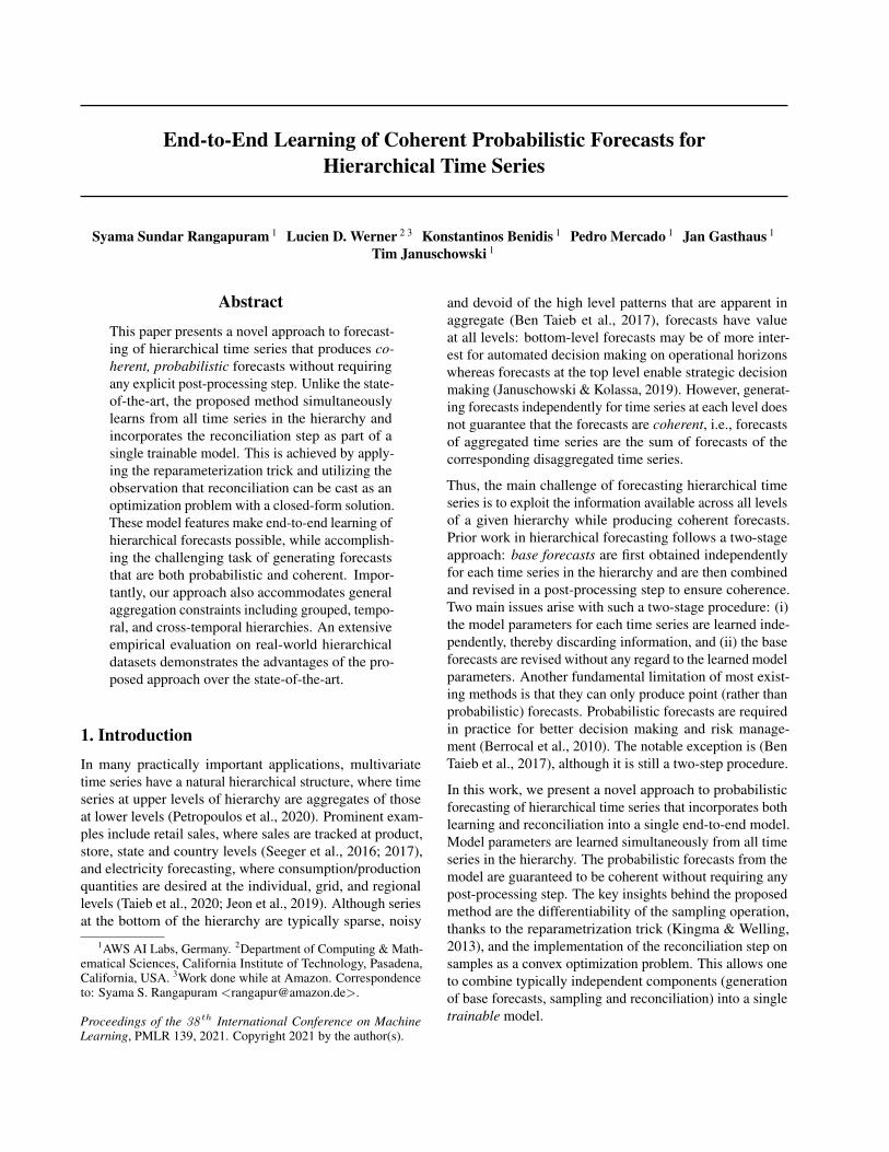
Figure 1. Example of hierarchical time series structure for n = 8time series with m = 5 bottom and r = 3 aggregated time series.

While our approach is fully general and can be used withany multivariate model, we show its empirical effective-ness via a specific multivariate, nonlinear autoregressivemodel, DeepVAR (Salinas et al., 2019), which exploits in-formation across all time series in the hierarchy to improveforecast accuracy.1 Moreover, since our model generatescoherent samples directly, it can be trained not only with thelog-likelihood loss but with any loss function that is of prac-tical interest. Our approach accommodates to incorporatecomplicated structural constraints on the forecasts via theuse of differentiable convex optimization layers (Agrawalet al., 2019a). For hierarchical reconciliation as we con-sider it here, this reduces to a simple closed-form solutionthus facilitating its inclusion as the last step of the trainablemodel.

In what follows, we provide the necessary background ofthe hierarchical forecasting problem and review the state-of-the art literature (Section 2). We then present our model inSection 3 and describe the training procedure. We provide athorough empirical evaluation on several real-world datasetsin Section 4 and conclude in Section 5.

2. Background and Related WorkA hierarchical time series is a multivariate time series thatsatisfies linear aggregation constraints. Such aggregationconstraints typically encode a tree hierarchy (see Figure 1)but need not necessarily. For example, grouped (Hyndmanet al., 2016), temporal (Athanasopoulos et al., 2017), andcross-temporal aggregations (Spiliotis et al., 2020) can alsobe expressed with linear constraints.

2.1. Preliminaries

Consider a time horizon t = 1, . . . , T . Let yt ∈ Rn denotethe values of a hierarchical time series at time t, with yt,i ∈R the value of the i-th (out of n) univariate time series. Herewe assume that the index i of the individual time series isgiven by the level-order traversal of the hierarchical treegoing from left to right at each level. Further, let xt,i ∈

1 In fact, we show in experiments that even without reconcilia-tion DeepVAR model outperforms classical hierarchical methods.

Rk be time varying covariate vectors associated to eachunivariate time series at time t, and xt := [xt,1, . . . ,xt,n] ∈Rk×n. We use the shorthand y1:T to denote the sequence{y1,y2, . . . ,yT }.

We refer to the time series at the leaf nodes of the hierarchyas bottom-level series and those of the remaining nodes asaggregated series. We also call a given set of forecasts forall time series in the hierarchy that are generated withoutheeding the aggregation constraint as base forecasts (not tobe confused with bottom-level). For notational conveniencewe split the vector of all series yt into m bottom entriesand r aggregated entries such that yt = [at bt]

> withat ∈ Rr and bt ∈ Rm. Clearly n = r + m. For anindividual hierarchy or grouping, an aggregation matrixS ∈ {0, 1}n×m is defined and the yt,bt, and S satisfy

yt = Sbt ⇔[at

bt

]=

[Ssum

Im

]bt, (1)

for every t. Ssum ∈ {0, 1}r×m is a summation matrix andIm is the m×m identity matrix. We also find it useful toequivalently represent (1) as

Ayt = 0, (2)

where A := [Ir | − Ssum] ∈ {0, 1}r×n, 0 is an r-vector ofzeros, and Ir is the r × r identity. Formulation (2) allowsfor a natural definition of forecast error (see below).

We illustrate our notation with the example in Figure 1.For this hierarchy, at = [y, y1, y2]>t ∈ R3 and bt =[b1, b2, b3, b4, b5]>t ∈ R5. The aggregation matrix S is

S =

[Ssum

I5

]=

1 1 1 1 11 1 0 0 00 0 1 1 1

I5

.

In hierarchical time series forecasting, one is typically in-terested in producing forecasts for all the time series in thehierarchy for a given number τ of future time steps after thepresent time T . Here τ is the length of the prediction or fore-cast horizon. The forecasts are either point predictions orprobabilistic in nature, in which case they can be representedas a set of Monte Carlo samples drawn from the forecastdistribution. For h ≤ τ we denote an h-period-ahead fore-cast sample by yT+h, with the entire set of samples thatcomprises the probabilistic forecast written as{yT+h}.

Clearly, an important aspect of hierarchical forecasting isthe requirement that the forecasts generated respect the ag-gregation constraint, which can be formalized as follows.Definition 2.1. Let S ⊆ Rn be a linear subspace defined as

S := {y|y ∈ null(A)}.


A point forecast yT+h is said to be coherent iff yT+h ∈ S.The coherency error of yT+h is defined as rT+h = AyT+h.Similarly, a probabilistic forecast represented as samples{yT+h} is coherent iff each of its samples is. Past observa-tions yt, t = 1, 2, . . . , T are coherent by construction.

Recent work Panagiotelis et al. (2020) proposes an alternatedefinition of coherence directly on probability densities.

2.2. Related Work

Existing approaches to hierarchical forecasting methodsmainly consider point forecasts with the notable excep-tion (Ben Taieb et al., 2017) tackling probabilistic fore-casts.2. In this section, we review several of the state-of-the-art methods.

Mean Forecast Combination & Reconciliation. Ap-proaches towards forecasting the means of hierarchical timeseries follow a two-step procedure: (i) forecast each timeseries independently to obtain base forecasts yT+h and(ii) produce revised forecasts yT+h through reconciliation.Given base forecasts yT+h, the methods in (Hyndmanet al., 2011; Wickramasuriya et al., 2019) obtain reconciledforecasts

yT+h = SP yT+h, (3)

where S is the aggregation matrix and P ∈ Rm×n is a ma-trix that depends on the choice of the hierarchical forecast-ing approach. When the method is bottom-up (BU), P =[0m×r|1m×m]. For top-down (TD), P = [pm×1|0m×n−1]where p is an m-vector summing to 1 that disaggregatesthe top-level series proportionally to the bottom level series.Middle-out (MO) can be analogously defined (Hyndman& Athanasopoulos, 2017). Connections to ensembling arepresented in (Hollyman et al., 2021).

The MinT method (Wickramasuriya et al., 2019) proposesreconciled forecasts using P =

(S>W−1h S

)−1 (S>W−1h

),

where Wh is the covariance matrix of the h-period-aheadforecast errors εT+h = yT+h − yT+h. It is shown thatwhen the yT+h are unbiased, this choice of P minimizesthe sum of variances of the forecast errors.

The advantages of the MinT approach are that its revisedforecasts are coherent by construction and the reconcilia-tion approach incorporates information from all levels ofhierarchy simultaneously. Disadvantages are the strong as-sumption of base forecasts to be unbiased and that the errorcovariance Wh is hard to obtain for general h.

The unbiasedness assumption in MinT is relaxed in(Ben Taieb & Koo, 2019). Rather than computing theminimum-variance revised forecasts, the authors seek to

2This is despite the general recognition of the practical im-portance of probabilistic forecasting for downstream applications(e.g., (Bose et al., 2017; Faloutsos et al., 2019)).

find the optimal bias-variance trade-off by solving an empir-ical risk minimization (ERM) problem. This method alsogenerates base forecasts, followed by reconciliation.

Van Erven & Cugliari (2015) follow the two-stage schemetoo. Their reconciliation approach is a weighted projectionof the base forecasts onto the coherent subspace S:

yt+h = arg minx

||Q(yt+h − x)||22s.t. x ∈ S ∩ B.

Q is a diagonal weight matrix that encodes knowledge/beliefabout the relative magnitudes of the base forecast errors foreach series in the hierarchy and B is a set of additionalconstraints to be imposed on the reconciled forecasts.

Probabilistic Methods. In contrast to the methods in theprevious section, Ben Taieb et al. (2017) consider forecast-ing probability distributions (Gneiting & Katzfuss, 2014)rather than just means (i.e., point forecasts). In particularthey estimate the conditional predictive CDF for each seriesi in the hierarchy:

Fi,T+h(yi | y1, . . . ,yT ) = P(yi,T+h ≤ yi | y1, . . . ,yT ).

Ben Taieb et al. (2017) start by generating independent fore-casts of the conditional marginal distributions (e.g., meanand variance from MinT). They obtain probabilistic fore-casts of the aggregate series by sampling from the bottom-level marginals of their children and re-ordering the samplesto match an empirical copula generated from the forecasterrors. Thus far, this method is a probabilistic “bottom-up”approach and emits coherent samples by construction. Toshare information between the levels, a combination step isperformed on the means of the learned marginal distribu-tions and the bottom-up samples are adjusted accordingly.

To the best of our knowledge, none of the existing ap-proaches to probabilistic forecasting take an end-to-endview. This introduces an opportunity to handle the trade-offbetween forecast accuracy and coherence better through asingle, joint model where reconciliation is performed along-side forecast learning. The flexibility of our frameworkmeans that we can take advantage of the increasingly richliterature on neural forecasting models, e.g., Benidis et al.(2020) provide an overview. Recent forecasting competi-tions have shown them to be highly effective (Makridakiset al., 2018; Bojer & Meldgaard, 2020; Makridakis et al.,to appear). Of particular relevance are multivariate, proba-bilistic, forecasting models (Rasul et al., 2021; de Bezenacet al., 2020; Salinas et al., 2019). These estimate the depen-dency structure in the time series panels explicitly and cannaturally be incorporated into our approach.


Θt

Hierarchical time series

yt

z ∼ 𝒩(0, I )

Multivariate forecastere.g., DeepVAR

ℓ (yt; Θct )

Sampling(includes transformation)

Projectione.g., closed form, DCL

Loss modele.g., log prob, CRPS, SSE

Learned parameters

e.g., μt, Σt

!yt+h

yt+h

yt+h

Θct

Sufficient statistics

e.g., quantiles, mean, variance

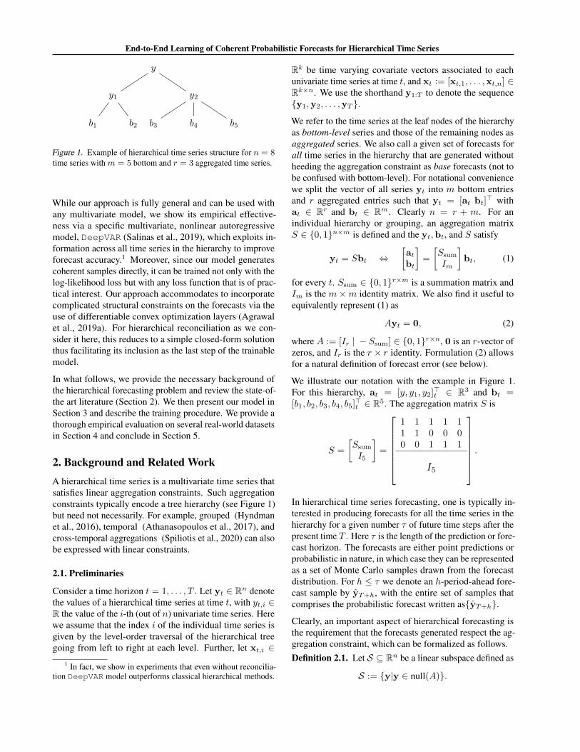
Figure 2. Model architecture. Hierarchical time series data is used to train a multivariate forecaster. Learned distribution parametersalong with the reparameterization trick allow this distribution to be sampled during training. Optionally, a nonlinear transformation of thesamples (e.g., normalizing flow) can account for data in a non-Gaussian domain. Samples are then projected to enforce coherency. Fromthe empirical distribution represented by the samples, sufficient statistics Θc

t can be computed and used to define an appropriate loss.

3. End-to-End Hierarchical ForecastingTwo primary components comprise our approach: (i) a fore-casting model that produces a multivariate forecast distri-bution over the prediction horizon; and (ii) a sampling &projection step where samples are drawn from the forecastdistribution, and are then projected onto the coherent sub-space. Figure 2 illustrates the architecture of the model.

It is important to note that when both of the above compo-nents are amenable to auto-differentiation, they constitute asingle global model whose parameters are learned end-to-end by minimizing a loss on the coherent samples directly.In particular, the sampling step can be differentiated us-ing the reparametrization trick (Kingma & Welling, 2013)and the projection step, which is an optimization problem,can be formed as a differentiable convex optimization layer(DCL) (Amos & Kolter, 2017; Agrawal et al., 2019a;b). Inthe setting of hierarchical and grouped time series, the opti-mization problem has a closed-form solution requiring onlya matrix-vector multiplication (with a pre-computable ma-trix) and hence is trivially differentiable. However, the pro-posed approach can handle more sophisticated constraintsthan those imposed by hierarchical setting via DCL.

3.1. Model

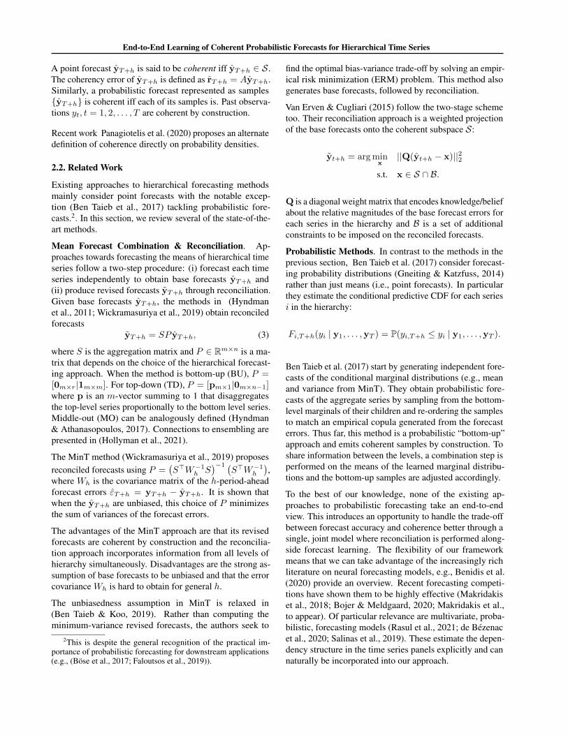
We now describe the instantiation of our model that is ex-plored in this work. We use DeepVAR (Salinas et al., 2019)as the base multivariate forecaster because of its simplicityand performance. A schematic of the full hierarchical modelis shown in Figure 3. The red dashed line represents theDeepVARmodel (described below) and the blue dashed linehighlights the sampling and projection steps. Once trained,the model produces coherent forecasts by construction.

3.1.1. DEEPVAR

DeepVAR is a multivariate, nonlinear generalization ofclassical autoregressive models (Salinas et al., 2019; 2020;Alexandrov et al., 2019).3 It uses a recurrent neural network(RNN) to exploit relationships across the entire history ofthe multivariate time series and is trained to learn parametersof the forecast distribution. More precisely, given a featurevector xt and the multivariate lags yt−1 ∈ Rn as inputs,DeepVAR assumes the predictive distribution at time step tis parameterized by Θt, which are the outputs of the RNN:

Θt = Ψ(xt,yt−1,ht−1; Φ). (4)

Here Ψ is a recurrent function of the RNN whose globalshared parameters are given by Φ and hidden state by ht−1.Typically, DeepVAR assumes that the forecast distributionis Gaussian in which case Θt = {µt,Σt}, where µt ∈ Rn

and Σt ∈ Sn+, although it can be extended to handle otherdistributions. The unknown parameters Φ are then learnedby the maximum likelihood principle given the training data.Note that for simplicity we specify only one lag yt−1 as theinput to the recurrent function but in the implementationlags are chosen from a lag set determined by the frequencyof the time series (Alexandrov et al., 2019).

In the hierarchical setting, the covariance matrix Σt capturesthe correlations imposed by the hierarchy as well as therelationships among the bottom-level time series. In ourexperience with industrial applications, we often find thatthe bottom-level time series are too sparse to learn anycovariance structure let alone more complicated nonlinearrelationships between them. Given this, we propose to learna diagonal covariance matrix Σt when producing the initialbase forecasts; if more flexibility is needed to capture thenonlinear relationships one could transform base forecastsusing normalizing flows (see Section 3.1.2). Note that thelinear relationships between the aggregated and bottom-

3Here we use the version without the Copula transformation.


yt−2,xt−1

ht−1

Θt−1

{yt−1}

P({yt−1})

{yt−1}

l(yt−1, {yt−1})

yt−1,xt

ht

Θt

{yt}

P({yt})

{yt}

l(yt, {yt})

yt,xt+1

ht+1

Θt+1

{yt+1}

P({yt+1})

{yt+1}

l(yt+1, {yt+1})

inputs

network

distr. params

base forecasts

reconciliation

coher. forecasts

loss

Figure 3. Specific instantiation of our approach withDeepVAR (Salinas et al., 2019) multivariate forecastingmodel (red boundary). Sampling and projection steps arehighlighted by the blue boundary.

level time series are enforced via projection.

Although we assume Σt is diagonal, this is not equivalentto learning independent models for each of the n time seriesin the hierarchy. In fact, the mean µt,i and the varianceΣt,(i,i) of the forecast distribution for each time series arepredicted by combining the lags of all time series yt−1and features xt in a nonlinear way using shared parametersΦ. In our experiments, we notice that this global learningalready produces much better results than the hierarchicalforecasting methods that do explicit reconciliation of theforecasts produced independently by univariate models.

3.1.2. SAMPLING AND PROJECTION

Next we describe how to generate coherent forecasts givendistribution parameters Θt = {µt,Σt} from the RNN. Tothis end, we first generate a set of N Monte Carlo samplesfrom the predicted distribution, {yt ∈ Rn} ∼ N (µt,Σt).Note that this sampling step is differentiable with a simplereparameterization of N (µt,Σt):

yt = µt + Σ1/2t z,

with z ∼ N (0, I). That is, given the samples from the stan-dard multivariate normal distribution, which are independentof the network parameters, the actual forecast samples aredeterministic functions of µt and Σt.

Optionally, in order to capture the nonlinear relationshipsamong the bottom-level time series, the generated samplescan be transformed using a learnable nonlinear transforma-tion. In this case, “forecasts” from the base model do notdirectly correspond to un-reconciled forecasts for the baseseries, but rather represent predictions of an unobservedlatent state. This is similar to the standard technique ofhandling non-Gaussian, nonlinear data by transforming itvia normalizing flows into a Gaussian space where tractablemethods can be applied. The main difference in our caseis that the nonlinear transformation need not be invertiblesince our loss is computed on the samples directly (seeSection 3.2).

Finally, we enforce coherence on the (transformed) samples{yt} obtained from the forecast distribution by solving thefollowing optimization problem:

yt = arg miny∈Rn

||y − yt||2

s.t. Ay = 0.(5)

Note that this is essentially projection onto the null spaceof A which can be computed with a closed-form projectionoperator:

M := I −A>(AA>)−1A. (6)

In other words, yt = M y ∈ S . Note that AA> is invertiblefor the hierarchical setting. M , which is time-invariant,can be computed offline once, prior to the start of training.In principle, the projection problem (5) can accommodateadditional convex constraints. Although this precludes thepossibility of a closed-form solution, the projection canbe implemented with a differentiable layer with the DCLframework (Agrawal et al., 2019a).

Accuracy-coherency trade-off. In practice, coherencyseems to improve accuracy (Wickramasuriya et al., 2019);our experiments confirm that as well. However, if thereis a trade-off, we can convert the constrained optimizationproblem (5) into unconstrained problem with a penalty pa-rameter (which would then be a hyperparameter giving thetrade-off). Values close to zero for this penalty parameterenforce no coherency and larger values make the predictionsmore coherent. Depending on the application, one could se-lect either the soft penalized version or the hard constrainedversion.

3.2. Training

The training of our hierarchical forecasting model is similarto DeepVAR except that the loss is directly computed on thecoherent predicted samples. Given a batch of training seriesY := {y1,y2, . . . ,yT }, where yt ∈ Rn, and associatedtime series features X := {x1,x2, . . . ,xT }, the likelihood


of the shared parameters Φ is given by

`(Φ) = p(Y ;X,Φ) =

T∏t=1

p(yt|y1:t−1; x1:t,Φ)

=

T∏t=1

p(yt|yt−1; xt,ht−1,Φ) =

T∏t=1

p(yt; Θt),

where Θt are the distribution parameters (Eq. (4)) predictedby the DeepVAR model.

In our hierarchical setting, the learnable parameters are stillgiven by Φ but the model outputs coherent Monte Carlosamples {yt} at each time step t. We are then able to com-pute sufficient statistics Θc

t on {yt} and define the followinglikelihood model:

`(Φ) =

T∏t=1

p(yt; Θct).

The exact distribution p(yt; Θct) can be chosen according to

the data. One can then maximize the likelihood to estimatethe parameters Φ. More importantly, we have the flexibilityto estimate the parameters Φ by optimizing any other lossfunction such as quantile loss, continuous ranked probabilityscore (Section 4 contains more details) or any of the metricstypically preferred in the forecasting community. This ispossible because any quantile of interest can be computedgiven sufficiently many samples (N large enough.)

In our model, the sampling step is differentiable as longas the distribution chosen allows for a suitable reparam-eterization where the random “noise” component of thedistribution can be separated from the deterministic valuesof the parameters. This is the case for several distributionsincluding Gaussian (Kingma & Welling, 2013), Gamma,log-Normal, Beta (Ruiz et al., 2016) and Student-t (Abiri& Ohlsson, 2019). Figurnov et al. (2018) present an alter-native approach to compute reparameterization gradientsshowing broader applicability to Student-t, Dirichlet andmixture distributions.

The projection step in our setting is just a matrix-vector mul-tiplication and poses no problem in automatically determin-ing the gradients. When reconciliation is a more involvedoptimization problem, as long as the problem can be writ-ten as a conic program, techniques such the ones presentedin (Agrawal et al., 2019b) enable automatic differentiation.

3.3. Prediction

Prediction is performed by unrolling the RNN step-by-stepover the prediction horizon as shown in Figure 4 (Salinaset al., 2019). Given an observed hierarchical time series{y1,y2, . . . ,yT }, we wish to predict its values for τ subse-quent periods. Starting with t = T + 1, we obtain forecast

yt−2,xt−1

ht−1

Θt−1

{yt−1}

P({yt−1})

{yt−1}

yt−1,xt

ht

Θt

{yt}

P({yt})

{yt}

yt,xt+1

ht+1

Θt+1

{yt+1}

P({yt+1})

{yt+1}

inputs

network

distr. params

base forecasts

reconciliation

coher. forecasts

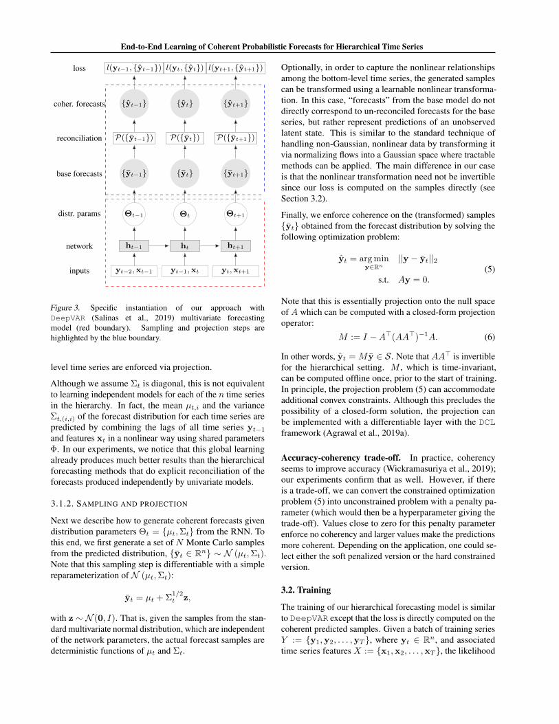
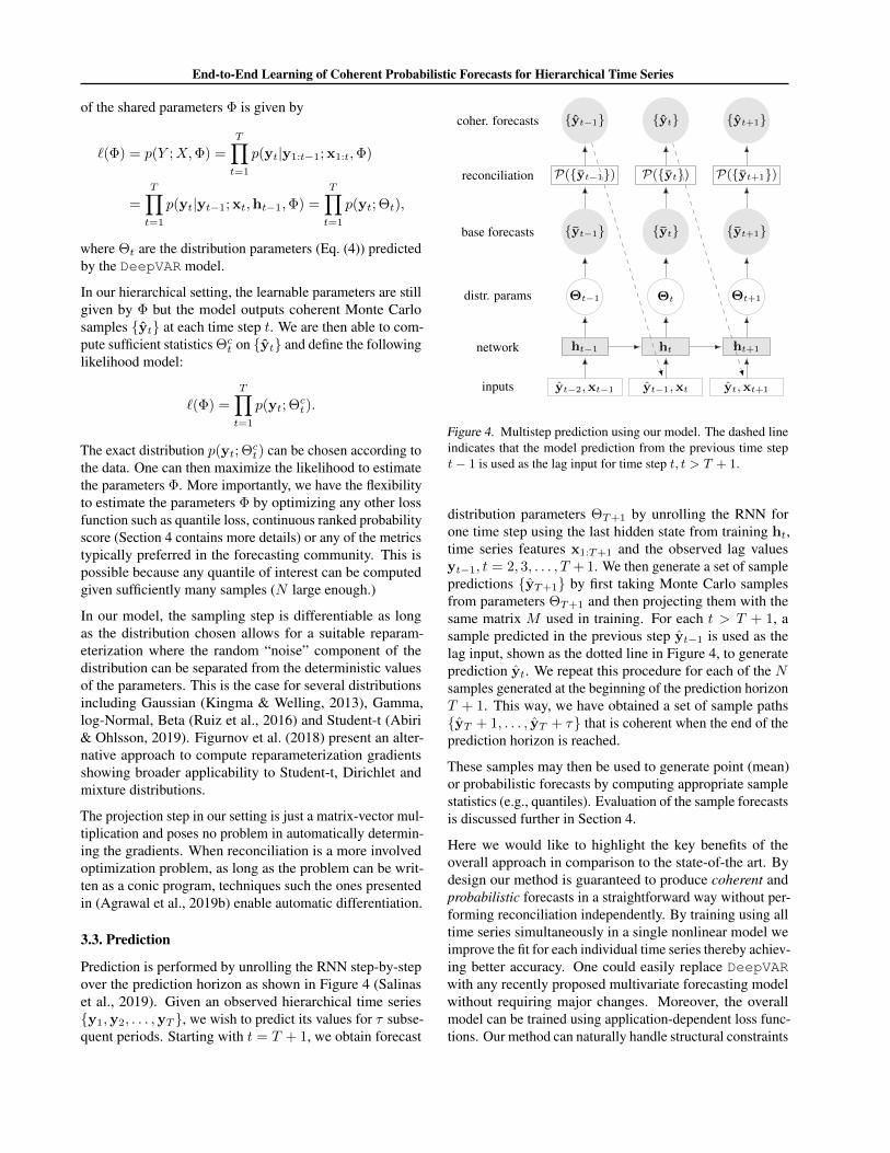
Figure 4. Multistep prediction using our model. The dashed lineindicates that the model prediction from the previous time stept− 1 is used as the lag input for time step t, t > T + 1.

distribution parameters ΘT+1 by unrolling the RNN forone time step using the last hidden state from training ht,time series features x1:T+1 and the observed lag valuesyt−1, t = 2, 3, . . . , T + 1. We then generate a set of samplepredictions {yT+1} by first taking Monte Carlo samplesfrom parameters ΘT+1 and then projecting them with thesame matrix M used in training. For each t > T + 1, asample predicted in the previous step yt−1 is used as thelag input, shown as the dotted line in Figure 4, to generateprediction yt. We repeat this procedure for each of the Nsamples generated at the beginning of the prediction horizonT + 1. This way, we have obtained a set of sample paths{yT + 1, . . . , yT + τ} that is coherent when the end of theprediction horizon is reached.

These samples may then be used to generate point (mean)or probabilistic forecasts by computing appropriate samplestatistics (e.g., quantiles). Evaluation of the sample forecastsis discussed further in Section 4.

Here we would like to highlight the key benefits of theoverall approach in comparison to the state-of-the art. Bydesign our method is guaranteed to produce coherent andprobabilistic forecasts in a straightforward way without per-forming reconciliation independently. By training using alltime series simultaneously in a single nonlinear model weimprove the fit for each individual time series thereby achiev-ing better accuracy. One could easily replace DeepVARwith any recently proposed multivariate forecasting modelwithout requiring major changes. Moreover, the overallmodel can be trained using application-dependent loss func-tions. Our method can naturally handle structural constraints


APPROACH NAIVEBU MINT ERM PERMBU-GTOP HIER-E2E (OURS)

PROBABILISTIC × × × X XMULTIVARIATE × × × X XIMPLICIT RECONCILIATION × × × × XSTRUCTURAL CONSTRAINTS (≥ 0) X X X × X

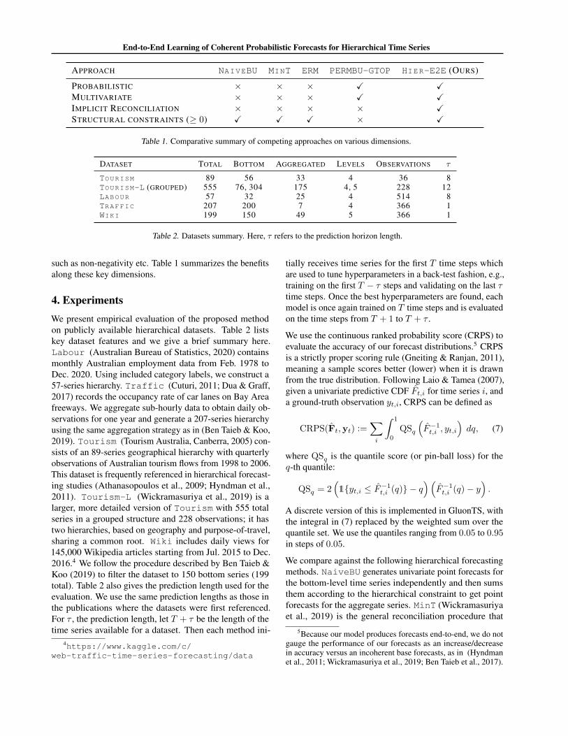
Table 1. Comparative summary of competing approaches on various dimensions.

DATASET TOTAL BOTTOM AGGREGATED LEVELS OBSERVATIONS τ

TOURISM 89 56 33 4 36 8TOURISM-L (GROUPED) 555 76, 304 175 4, 5 228 12LABOUR 57 32 25 4 514 8TRAFFIC 207 200 7 4 366 1WIKI 199 150 49 5 366 1

Table 2. Datasets summary. Here, τ refers to the prediction horizon length.

such as non-negativity etc. Table 1 summarizes the benefitsalong these key dimensions.

4. ExperimentsWe present empirical evaluation of the proposed methodon publicly available hierarchical datasets. Table 2 listskey dataset features and we give a brief summary here.Labour (Australian Bureau of Statistics, 2020) containsmonthly Australian employment data from Feb. 1978 toDec. 2020. Using included category labels, we construct a57-series hierarchy. Traffic (Cuturi, 2011; Dua & Graff,2017) records the occupancy rate of car lanes on Bay Areafreeways. We aggregate sub-hourly data to obtain daily ob-servations for one year and generate a 207-series hierarchyusing the same aggregation strategy as in (Ben Taieb & Koo,2019). Tourism (Tourism Australia, Canberra, 2005) con-sists of an 89-series geographical hierarchy with quarterlyobservations of Australian tourism flows from 1998 to 2006.This dataset is frequently referenced in hierarchical forecast-ing studies (Athanasopoulos et al., 2009; Hyndman et al.,2011). Tourism-L (Wickramasuriya et al., 2019) is alarger, more detailed version of Tourism with 555 totalseries in a grouped structure and 228 observations; it hastwo hierarchies, based on geography and purpose-of-travel,sharing a common root. Wiki includes daily views for145,000 Wikipedia articles starting from Jul. 2015 to Dec.2016.4 We follow the procedure described by Ben Taieb &Koo (2019) to filter the dataset to 150 bottom series (199total). Table 2 also gives the prediction length used for theevaluation. We use the same prediction lengths as those inthe publications where the datasets were first referenced.For τ , the prediction length, let T + τ be the length of thetime series available for a dataset. Then each method ini-

4https://www.kaggle.com/c/web-traffic-time-series-forecasting/data

tially receives time series for the first T time steps whichare used to tune hyperparameters in a back-test fashion, e.g.,training on the first T − τ steps and validating on the last τtime steps. Once the best hyperparameters are found, eachmodel is once again trained on T time steps and is evaluatedon the time steps from T + 1 to T + τ .

We use the continuous ranked probability score (CRPS) toevaluate the accuracy of our forecast distributions.5 CRPSis a strictly proper scoring rule (Gneiting & Ranjan, 2011),meaning a sample scores better (lower) when it is drawnfrom the true distribution. Following Laio & Tamea (2007),given a univariate predictive CDF Ft,i for time series i, anda ground-truth observation yt,i, CRPS can be defined as

CRPS(Ft,yt) :=∑i

∫ 1

0

QSq

(F−1t,i , yt,i

)dq, (7)

where QSq is the quantile score (or pin-ball loss) for theq-th quantile:

QSq = 2(1{yt,i ≤ F−1t,i (q)} − q

)(F−1t,i (q)− y

).

A discrete version of this is implemented in GluonTS, withthe integral in (7) replaced by the weighted sum over thequantile set. We use the quantiles ranging from 0.05 to 0.95in steps of 0.05.

We compare against the following hierarchical forecastingmethods. NaiveBU generates univariate point forecasts forthe bottom-level time series independently and then sumsthem according to the hierarchical constraint to get pointforecasts for the aggregate series. MinT (Wickramasuriyaet al., 2019) is the general reconciliation procedure that

5Because our model produces forecasts end-to-end, we do notgauge the performance of our forecasts as an increase/decreasein accuracy versus an incoherent base forecasts, as in (Hyndmanet al., 2011; Wickramasuriya et al., 2019; Ben Taieb et al., 2017).


method Labour Traffic Tourism Tourism-L Wiki

ARIMA-NaiveBU 0.0453 0.0808 0.1138 0.1741 0.3772ETS-NaiveBU 0.0432 0.0665 0.1008 0.1690 0.4673

ARIMA-MinT-shr 0.0467 0.0770 0.1171 0.1609 0.2467ARIMA-MinT-ols 0.0463 0.1116 0.1195 0.1729 0.2782ETS-MinT-shr 0.0455 0.0963 0.1013 0.1627 0.3622ETS-MinT-ols 0.0459 0.1110 0.1002 0.1668 0.2702ARIMA-ERM 0.0399 0.0466 0.5887 0.5635 0.2206ETS-ERM 0.0456 0.1027 2.3755 0.5080 0.2217

PERMBU-MINT 0.0393±0.0002 0.0677±0.0061 0.0771±0.0001 — 0.2812±0.0240Hier-E2E (Ours) 0.0340±0.0088 0.0376±0.0060 0.0834±0.0052 0.1520±0.0032 0.2038±0.0110

ablationstudy

{DeepVAR 0.0382±0.0045 0.0400±0.0026 0.0925±0.0022 0.1581±0.0102 0.2294±0.0158DeepVAR+ 0.0433±0.0079 0.0434±0.0049 0.0958±0.0062 0.1882±0.0242 0.2439±0.0224

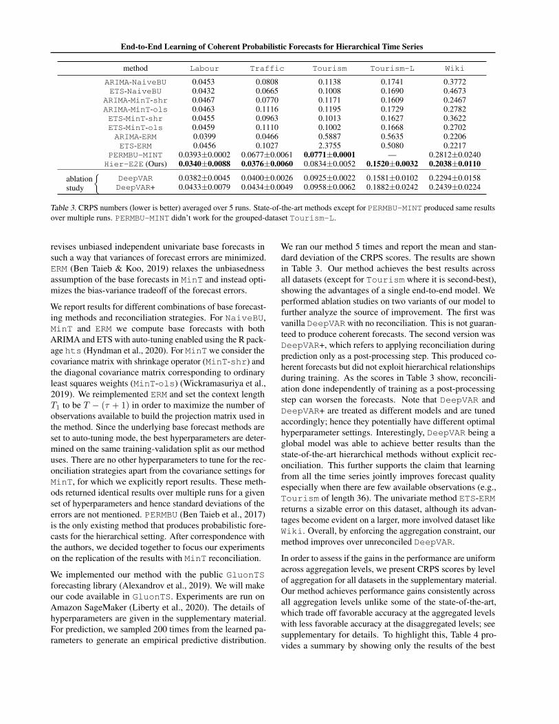
Table 3. CRPS numbers (lower is better) averaged over 5 runs. State-of-the-art methods except for PERMBU-MINT produced same resultsover multiple runs. PERMBU-MINT didn’t work for the grouped-dataset Tourism-L.

revises unbiased independent univariate base forecasts insuch a way that variances of forecast errors are minimized.ERM (Ben Taieb & Koo, 2019) relaxes the unbiasednessassumption of the base forecasts in MinT and instead opti-mizes the bias-variance tradeoff of the forecast errors.

We report results for different combinations of base forecast-ing methods and reconciliation strategies. For NaiveBU,MinT and ERM we compute base forecasts with bothARIMA and ETS with auto-tuning enabled using the R pack-age hts (Hyndman et al., 2020). For MinT we consider thecovariance matrix with shrinkage operator (MinT-shr) andthe diagonal covariance matrix corresponding to ordinaryleast squares weights (MinT-ols) (Wickramasuriya et al.,2019). We reimplemented ERM and set the context lengthT1 to be T − (τ + 1) in order to maximize the number ofobservations available to build the projection matrix used inthe method. Since the underlying base forecast methods areset to auto-tuning mode, the best hyperparameters are deter-mined on the same training-validation split as our methoduses. There are no other hyperparameters to tune for the rec-onciliation strategies apart from the covariance settings forMinT, for which we explicitly report results. These meth-ods returned identical results over multiple runs for a givenset of hyperparameters and hence standard deviations of theerrors are not mentioned. PERMBU (Ben Taieb et al., 2017)is the only existing method that produces probabilistic fore-casts for the hierarchical setting. After correspondence withthe authors, we decided together to focus our experimentson the replication of the results with MinT reconciliation.

We implemented our method with the public GluonTSforecasting library (Alexandrov et al., 2019). We will makeour code available in GluonTS. Experiments are run onAmazon SageMaker (Liberty et al., 2020). The details ofhyperparameters are given in the supplementary material.For prediction, we sampled 200 times from the learned pa-rameters to generate an empirical predictive distribution.

We ran our method 5 times and report the mean and stan-dard deviation of the CRPS scores. The results are shownin Table 3. Our method achieves the best results acrossall datasets (except for Tourism where it is second-best),showing the advantages of a single end-to-end model. Weperformed ablation studies on two variants of our model tofurther analyze the source of improvement. The first wasvanilla DeepVAR with no reconciliation. This is not guaran-teed to produce coherent forecasts. The second version wasDeepVAR+, which refers to applying reconciliation duringprediction only as a post-processing step. This produced co-herent forecasts but did not exploit hierarchical relationshipsduring training. As the scores in Table 3 show, reconcili-ation done independently of training as a post-processingstep can worsen the forecasts. Note that DeepVAR andDeepVAR+ are treated as different models and are tunedaccordingly; hence they potentially have different optimalhyperparameter settings. Interestingly, DeepVAR being aglobal model was able to achieve better results than thestate-of-the-art hierarchical methods without explicit rec-onciliation. This further supports the claim that learningfrom all the time series jointly improves forecast qualityespecially when there are few available observations (e.g.,Tourism of length 36). The univariate method ETS-ERMreturns a sizable error on this dataset, although its advan-tages become evident on a larger, more involved dataset likeWiki. Overall, by enforcing the aggregation constraint, ourmethod improves over unreconciled DeepVAR.

In order to assess if the gains in the performance are uniformacross aggregation levels, we present CRPS scores by levelof aggregation for all datasets in the supplementary material.Our method achieves performance gains consistently acrossall aggregation levels unlike some of the state-of-the-art,which trade off favorable accuracy at the aggregated levelswith less favorable accuracy at the disaggregated levels; seesupplementary for details. To highlight this, Table 4 pro-vides a summary by showing only the results of the best


Dataset Level Hier-E2E(Ours) DeepVAR DeepVAR+ Best of Competing Methods

Labour1 0.0311±0.0120 0.0352±0.0079 0.0416±0.0094 0.0406±0.0002 (PERMBU-MINT)2 0.0336±0.0089 0.0374±0.0051 0.0437±0.0078 0.0389±0.0002(PERMBU-MINT)3 0.0336±0.0082 0.0383±0.0038 0.0432±0.0076 0.0382±0.0002(PERMBU-MINT)4 0.0378±0.0060 0.0417±0.0038 0.0448±0.0066 0.0397±0.0003(PERMBU-MINT)

Traffic1 0.0184±0.0091 0.0225±0.0109 0.0250±0.0082 0.0087(ARIMA-ERM)2 0.0181±0.0086 0.0204±0.0044 0.0244±0.0063 0.0112(ARIMA-ERM)3 0.0223±0.0072 0.0190±0.0031 0.0259±0.0054 0.0255(ARIMA-ERM)4 0.0914±0.0024 0.0982±0.0012 0.0982±0.0017 0.1410(ARIMA-ERM)

Tourism1 0.0402±0.0040 0.0519±0.0057 0.0508±0.0085 0.0472±0.0012 (PERMBU-MINT)2 0.0658±0.0084 0.0755±0.0011 0.0750±0.0066 0.0605±0.0006 (PERMBU-MINT)3 0.1053±0.0053 0.1134±0.0049 0.1180±0.0053 0.0903±0.0006 (PERMBU-MINT)4 0.1223±0.0039 0.1294±0.0060 0.1393±0.0048 0.1106±0.0005 (PERMBU-MINT)

Tourism-L

1 0.0810±0.0053 0.1029±0.0188 0.1214±0.0360 0.0438 (ARIMA-MinT-shr)2 (geo.) 0.1030±0.0030 0.1076±0.0119 0.1364±0.0299 0.0816 (ARIMA-MinT-shr)3 (geo.) 0.1361±0.0024 0.1407±0.0081 0.1713±0.0243 0.1433(ARIMA-MinT-shr)4 (geo.) 0.1752±0.0026 0.1741±0.0066 0.2079±0.0215 0.2036(ARIMA-MinT-shr)

2 (trav.) 0.1027±0.0062 0.1100±0.0139 0.1370±0.0289 0.0830 (ARIMA-MinT-shr)3 (trav.) 0.1403±0.0047 0.1485±0.0099 0.1776±0.0221 0.1479 (ARIMA-MinT-shr)4 (trav.) 0.2050±0.0028 0.2078±0.0076 0.2435±0.0170 0.2437(ARIMA-MinT-shr)5 (trav.) 0.2727±0.0017 0.2731±0.0066 0.3108±0.0164 0.3406(ARIMA-MinT-shr)

Wiki

1 0.0419±0.0285 0.0905±0.0323 0.0755±0.0165 0.1558 (ETS-ERM)2 0.1045±0.0151 0.1418±0.0249 0.1289±0.0171 0.1614 (ETS-ERM)3 0.2292±0.0108 0.2597±0.0150 0.2583±0.0281 0.2010(ETS-ERM)4 0.2716±0.0091 0.2886±0.0112 0.3108±0.0298 0.2399(ETS-ERM)5 0.3720±0.0150 0.3664±0.0068 0.4460±0.0271 0.3507(ETS-ERM)

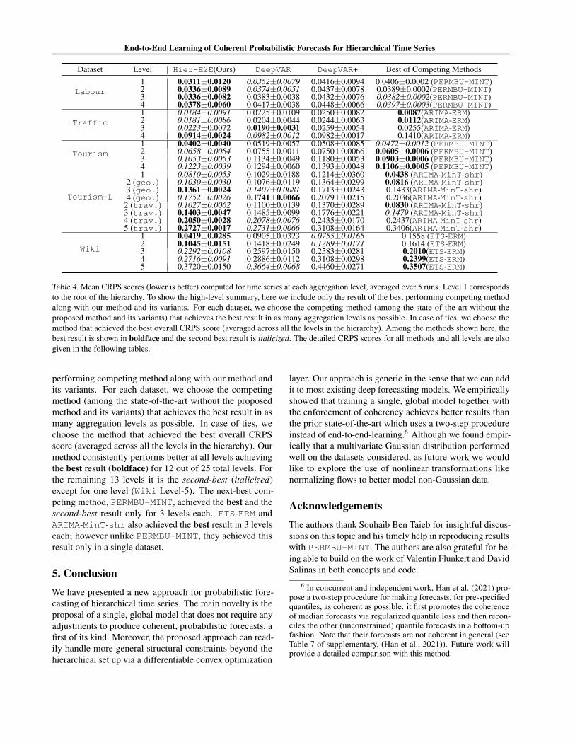
Table 4. Mean CRPS scores (lower is better) computed for time series at each aggregation level, averaged over 5 runs. Level 1 correspondsto the root of the hierarchy. To show the high-level summary, here we include only the result of the best performing competing methodalong with our method and its variants. For each dataset, we choose the competing method (among the state-of-the-art without theproposed method and its variants) that achieves the best result in as many aggregation levels as possible. In case of ties, we choose themethod that achieved the best overall CRPS score (averaged across all the levels in the hierarchy). Among the methods shown here, thebest result is shown in boldface and the second best result is italicized. The detailed CRPS scores for all methods and all levels are alsogiven in the following tables.

performing competing method along with our method andits variants. For each dataset, we choose the competingmethod (among the state-of-the-art without the proposedmethod and its variants) that achieves the best result in asmany aggregation levels as possible. In case of ties, wechoose the method that achieved the best overall CRPSscore (averaged across all the levels in the hierarchy). Ourmethod consistently performs better at all levels achievingthe best result (boldface) for 12 out of 25 total levels. Forthe remaining 13 levels it is the second-best (italicized)except for one level (Wiki Level-5). The next-best com-peting method, PERMBU-MINT, achieved the best and thesecond-best result only for 3 levels each. ETS-ERM andARIMA-MinT-shr also achieved the best result in 3 levelseach; however unlike PERMBU-MINT, they achieved thisresult only in a single dataset.

5. ConclusionWe have presented a new approach for probabilistic fore-casting of hierarchical time series. The main novelty is theproposal of a single, global model that does not require anyadjustments to produce coherent, probabilistic forecasts, afirst of its kind. Moreover, the proposed approach can read-ily handle more general structural constraints beyond thehierarchical set up via a differentiable convex optimization

layer. Our approach is generic in the sense that we can addit to most existing deep forecasting models. We empiricallyshowed that training a single, global model together withthe enforcement of coherency achieves better results thanthe prior state-of-the-art which uses a two-step procedureinstead of end-to-end-learning.6 Although we found empir-ically that a multivariate Gaussian distribution performedwell on the datasets considered, as future work we wouldlike to explore the use of nonlinear transformations likenormalizing flows to better model non-Gaussian data.

AcknowledgementsThe authors thank Souhaib Ben Taieb for insightful discus-sions on this topic and his timely help in reproducing resultswith PERMBU-MINT. The authors are also grateful for be-ing able to build on the work of Valentin Flunkert and DavidSalinas in both concepts and code.

6 In concurrent and independent work, Han et al. (2021) pro-pose a two-step procedure for making forecasts, for pre-specifiedquantiles, as coherent as possible: it first promotes the coherenceof median forecasts via regularized quantile loss and then recon-ciles the other (unconstrained) quantile forecasts in a bottom-upfashion. Note that their forecasts are not coherent in general (seeTable 7 of supplementary, (Han et al., 2021)). Future work willprovide a detailed comparison with this method.


ReferencesAbiri, N. and Ohlsson, M. Variational auto-encoders with

student’s t-prior. In Proceedings, 27th European Sym-posium on Artificial Neural Networks, ComputationalIntelligence and Machine Learning (ESANN 2019), pp.415–420, Bruges, 2019.

Agrawal, A., Amos, B., Barratt, S., Boyd, S., Diamond, S.,and Kolter, Z. Differentiable convex optimization layers.arXiv preprint arXiv:1910.12430, 2019a.

Agrawal, A., Barratt, S., Boyd, S., Busseti, E., and Moursi,W. M. Differentiating through a cone program. arXivpreprint arXiv:1904.09043, 2019b.

Alexandrov, A., Benidis, K., Bohlke-Schneider, M.,Flunkert, V., Gasthaus, J., Januschowski, T., Maddix,D. C., Rangapuram, S., Salinas, D., Schulz, J., et al. Glu-onTS: Probabilistic Time Series Models in Python. JMLR,2019.

Amos, B. and Kolter, J. Z. Optnet: Differentiable opti-mization as a layer in neural networks. In InternationalConference on Machine Learning, pp. 136–145. PMLR,2017.

Athanasopoulos, G., Ahmed, R. A., and Hyndman, R. J.Hierarchical forecasts for australian domestic tourism. In-ternational Journal of Forecasting, 25(1):146–166, 2009.

Athanasopoulos, G., Hyndman, R. J., Kourentzes, N., andPetropoulos, F. Forecasting with temporal hierarchies.European Journal of Operational Research, 262(1):60–74, 2017.

Australian Bureau of Statistics. LabourForce, Australia, Dec 2020. URL https://www.abs.gov.au/statistics/labour/employment-and-unemployment/labour-force-australia/latest-release.Accessed on 01.12.2021.

Ben Taieb, S. and Koo, B. Regularized regression for hi-erarchical forecasting without unbiasedness conditions.In Proceedings of the 25th ACM SIGKDD InternationalConference on Knowledge Discovery & Data Mining, pp.1337–1347, 2019.

Ben Taieb, S., Taylor, J. W., and Hyndman, R. J. Coherentprobabilistic forecasts for hierarchical time series. InInternational Conference on Machine Learning, pp. 3348–3357, 2017.

Benidis, K., Rangapuram, S. S., Flunkert, V., Wang,B., Maddix, D., Turkmen, C., Gasthaus, J., Bohlke-Schneider, M., Salinas, D., Stella, L., Callot, L., andJanuschowski, T. Neural forecasting: Introduction and

literature overview. arXiv preprint arXiv:2004.10240,2020.

Berrocal, V. J., Raftery, A. E., Gneiting, T., and Steed, R. C.Probabilistic weather forecasting for winter road mainte-nance. Journal of the American Statistical Association,105(490):522–537, 2010.

Bojer, C. S. and Meldgaard, J. P. Kaggle forecast-ing competitions: An overlooked learning opportu-nity. International Journal of Forecasting, Sep 2020.ISSN 0169-2070. doi: 10.1016/j.ijforecast.2020.07.007. URL http://dx.doi.org/10.1016/j.ijforecast.2020.07.007.

Bose, J.-H., Flunkert, V., Gasthaus, J., Januschowski, T.,Lange, D., Salinas, D., Schelter, S., Seeger, M., and Wang,Y. Probabilistic demand forecasting at scale. Proceedingsof the VLDB Endowment, 10(12):1694–1705, 2017.

Cuturi, M. Fast global alignment kernels. In Proceedings ofthe 28th International Conference on Machine Learning(ICML 2011), 2011.

de Bezenac, E., Rangapuram, S. S., Benidis, K., Bohlke-Schneider, M., Kurle, R., Stella, L., Hasson, H., Gallinari,P., and Januschowski, T. Normalizing kalman filters formultivariate time series analysis. In Advances in Neu-ral Information Processing Systems 33: Annual Confer-ence on Neural Information Processing Systems 2020,NeurIPS 2020, December 6-12, 2020, virtual, 2020.

Dua, D. and Graff, C. UCI machine learning repository,2017. URL http://archive.ics.uci.edu/ml.

Faloutsos, C., Gasthaus, J., Januschowski, T., and Wang, Y.Classical and contemporary approaches to big time seriesforecasting. In Proceedings of the 2019 InternationalConference on Management of Data, SIGMOD ’19, NewYork, NY, USA, 2019. ACM.

Figurnov, M., Mohamed, S., and Mnih, A. Implicitreparameterization gradients. In Bengio, S., Wallach,H., Larochelle, H., Grauman, K., Cesa-Bianchi, N.,and Garnett, R. (eds.), Advances in Neural InformationProcessing Systems, volume 31, pp. 441–452. Curran As-sociates, Inc., 2018. URL https://proceedings.neurips.cc/paper/2018/file/92c8c96e4c37100777c7190b76d28233-Paper.pdf.

Gneiting, T. and Katzfuss, M. Probabilistic forecasting.Annual Review of Statistics and Its Application, 1:125–151, 2014.

Gneiting, T. and Ranjan, R. Comparing density forecasts us-ing threshold-and quantile-weighted scoring rules. Jour-nal of Business & Economic Statistics, 29(3):411–422,2011.


Han, X., Dasgupta, S., and Ghosh, J. Simultaneously recon-ciled quantile forecasting of hierarchically related timeseries. In Proceedings of The 24th International Con-ference on Artificial Intelligence and Statistics, volume130 of Proceedings of Machine Learning Research, pp.190–198. PMLR, 13–15 Apr 2021.

Hollyman, R., Petropoulos, F., and Tipping, M. E. Under-standing forecast reconciliation. European Journal ofOperational Research, 2021.

Hyndman, R., Lee, A., Wang, E., and Wickramasuriya,S. hts: Hierarchical and Grouped Time Series,2020. URL https://CRAN.R-project.org/package=hts. R package version 6.0.1.

Hyndman, R. J. and Athanasopoulos, G. Forecasting: Prin-ciples and practice. www. otexts. org/fpp., 987507109,2017.

Hyndman, R. J., Ahmed, R. A., Athanasopoulos, G., andShang, H. L. Optimal combination forecasts for hierarchi-cal time series. Computational statistics & data analysis,55(9):2579–2589, 2011.

Hyndman, R. J., Lee, A. J., and Wang, E. Fast computationof reconciled forecasts for hierarchical and grouped timeseries. Computational statistics & data analysis, 97:16–32, 2016.

Januschowski, T. and Kolassa, S. A classification of busi-ness forecasting problems. Foresight: The InternationalJournal of Applied Forecasting, 52:36–43, 2019.

Jeon, J., Panagiotelis, A., and Petropoulos, F. Probabilisticforecast reconciliation with applications to wind powerand electric load. European Journal of Operational Re-search, 279(2):364–379, 2019.

Kingma, D. P. and Welling, M. Auto-encoding variationalbayes. arXiv preprint arXiv:1312.6114, 2013.

Laio, F. and Tamea, S. Verification tools for probabilisticforecasts of continuous hydrological variables. Hydrologyand Earth System Sciences, 11(4):1267–1277, 2007.

Liberty, E., Karnin, Z., Xiang, B., Rouesnel, L., Coskun,B., Nallapati, R., Delgado, J., Sadoughi, A., Astashonok,Y., Das, P., Balioglu, C., Chakravarty, S., Jha, M., Gau-tier, P., Arpin, D., Januschowski, T., Flunkert, V., Wang,Y., Gasthaus, J., Stella, L., Rangapuram, S., Salinas, D.,Schelter, S., and Smola, A. Elastic machine learningalgorithms in amazon sagemaker. In Proceedings of the2020 ACM SIGMOD International Conference on Man-agement of Data, SIGMOD ’20, pp. 731–737, New York,NY, USA, 2020. Association for Computing Machinery.ISBN 9781450367356.

Makridakis, S., Spiliotis, E., and Assimakopoulos,V. The m4 competition: Results, findings, con-clusion and way forward. International Journalof Forecasting, 2018. ISSN 0169-2070. doi:https://doi.org/10.1016/j.ijforecast.2018.06.001. URLhttp://www.sciencedirect.com/science/article/pii/S0169207018300785.

Makridakis, S., Spiliotis, E., and Assimakopoulos, V. Them5 accuracy competition: Results, findings and conclu-sions. International Journal of Forecasting, to appear.

Panagiotelis, A., Gamakumara, P., Athanasopoulos, G., andHyndman, R. J. Probabilistic Forecast Reconciliation:Properties, Evaluation and Score Optimisation. Technicalreport, 2020.

Petropoulos, F. et al. Forecasting: theory and practice. arXivpreprint arXiv:2012.03854, 2020.

Rasul, K., Sheikh, A.-S., Schuster, I., Bergmann, U., andVollgraf, R. Multivariate probabilistic time series fore-casting via conditioned normalizing flows, 2021.

Ruiz, F. R., Titsias RC AUEB, M., and Blei, D. Thegeneralized reparameterization gradient. In Lee, D.,Sugiyama, M., Luxburg, U., Guyon, I., and Garnett,R. (eds.), Advances in Neural Information ProcessingSystems, volume 29, pp. 460–468. Curran Asso-ciates, Inc., 2016. URL https://proceedings.neurips.cc/paper/2016/file/f718499c1c8cef6730f9fd03c8125cab-Paper.pdf.

Salinas, D., Bohlke-Schneider, M., Callot, L., Medico, R.,and Gasthaus, J. High-dimensional multivariate forecast-ing with low-rank gaussian copula processes. Advancesin neural information processing systems, 32:6827–6837,2019.

Salinas, D., Flunkert, V., Gasthaus, J., and Januschowski,T. Deepar: Probabilistic forecasting with autoregressiverecurrent networks. International Journal of Forecasting,36(3):1181–1191, 2020.

Seeger, M., Rangapuram, S., Wang, Y., Salinas, D.,Gasthaus, J., Januschowski, T., and Flunkert, V. Ap-proximate bayesian inference in linear state space modelsfor intermittent demand forecasting at scale, 2017.

Seeger, M. W., Salinas, D., and Flunkert, V. Bayesianintermittent demand forecasting for large inventories. InAdvances in Neural Information Processing Systems, pp.4646–4654, 2016.

Spiliotis, E., Petropoulos, F., Kourentzes, N., and Assi-makopoulos, V. Cross-temporal aggregation: Improvingthe forecast accuracy of hierarchical electricity consump-tion. Applied Energy, 261:114339, 2020.


Taieb, S. B., Taylor, J. W., and Hyndman, R. J. Hierarchi-cal probabilistic forecasting of electricity demand withsmart meter data. Journal of the American StatisticalAssociation, 0(0):1–17, 2020.

Tourism Australia, Canberra. Tourism Research Australia(2005), Travel by Australians, Sep 2005. Accessedat https://robjhyndman.com/publications/hierarchical-tourism/.

Van Erven, T. and Cugliari, J. Game-theoretically optimalreconciliation of contemporaneous hierarchical time se-ries forecasts. In Modeling and stochastic learning forforecasting in high dimensions, pp. 297–317. Springer,2015.

Wickramasuriya, S. L., Athanasopoulos, G., and Hynd-man, R. J. Optimal forecast reconciliation for hier-archical and grouped time series through trace min-imization. Journal of the American Statistical As-sociation, 114(526):804–819, 2019. doi: 10.1080/01621459.2018.1448825. URL https://doi.org/10.1080/01621459.2018.1448825.

end-to-end learning of coherent probabilistic forecasts

Documents