1

AIM 2012

Energy balance and numerical simulation of microseismicity induced by hydraulic fracturing

David W. Eaton* and Neda Boroumand

Department of Geoscience University of Calgary

* Currently at University of Bristol

Acknowledgements:

Sponsors of the Microseismic Industry Consortium

Nexen Inc. for data

2

AIM 2012

1. Role of microseismic monitoring in hydraulic fracturing for unconventional oil resource development

2. Energy balance: radiated seismic energy versus frac energy inputs/outputs

3. Numerical simulation of frac-induced microseismicity, based on crack-tip stress and Coulomb Stress field

Outline

3

AIM 2012

What is hydraulic fracturing?

• High-pressure fluids are injected to create tensile fractures, in order to enhance permeability of hydrocarbon-bearing formations

• This is followed by injection of proppant (e.g. sand) to hold fractures open• Typically implemented in multiple stages within a horizontal wellbore, often

many drilled from a single pad

http://www.capp.ca

4

AIM 2012

Pettitt, 2010

Hydraulic Fracturing:Role of Microseismic Monitoring• Typically a string of

downhole geophones and/or surface array

• Real-time monitoring to fine-tune injection program, diagnose issues

• Post-frac analysis to assess stimulation program

5

AIM 2012

Input vs Output EnergyInjection Energy (EI)

Pressure

Time

Fracture Energy (EF)

Strain Energy (ES)http://www.engineeringarchives.com

Radiated Seismic Energy (ER)

Other (i.e. friction/thermal,

hydrostatic, leak-off, etc.)

Rate

6

AIM 2012

Pressure (P)

Time

Rate (Q)

Injection Energy

Where Q(t) = injection rate, P(t) = surface treatment pressure

t1 & t2 are start and end times of treatment

7

AIM 2012

Fracture Energy

where <Pd> is the average downhole pressure, <AF> is

the single-sided surface area and is the average fracture width (Walter and Brune, JGR, 1993)

8

AIM 2012

Radiated Seismic Energy

Kanamori, 1977

where M0 is moment magnitude, and ES is in Joules

… but note missing data in G-R plot

9

AIM 2012

Case Study

• 10 frac stages • Microseismic

event locations and magnitudes were provided (geometry was measured)

• Pumping data provided

10

AIM 2012

Energy per event

Energy per bin

Joul

esJo

ules

Total predicted energy: 4.63e+6JTotal observed energy: 1.81e+5J

Ratio = 25.6

Based on Hanks and Kanamori (1979)

• b = 1.57, small magnitude events contribute more to total seismic energy

• If b < 1.5 then more total energy in larger bins

• If b > 1.5, then more energy in successively smaller bins

b-value correction

11

AIM 2012

Injection Energy Fracture Energy Seismic EnergyWell/Formation Name Stage (KJoules) (KJoules) (KJoules) % Fracture Energy % Seismic Energy

Well #1 (Otter Park) Stage 18 192,647,400.00 29,168,562.50 9,996.79 15 0.03Stage 19 165,301,920.00 27,188,525.00 19,508.12 16 0.07Stage 20 154,350,000.00 22,137,500.00 4,641.58 14 0.02

Well # 2 (Otter Park) Stage 19 163,838,400.00 40,035,000.00 9,230.97 24 0.02Well # 3 (Muskwa) Stage 13 140,829,120.00 34,979,600.00 28,055.40 25 0.08

Stage 14 144,942,000.00 37,900,800.00 25,532.75 26 0.07Stage 15 162,035,040.00 66,409,750.00 32,141.91 41 0.05Stage 16 143,100,000.00 53,845,000.00 32,845.77 38 0.06

Well # 3 (Muskwa) Stage 17 156,017,100.00 22,160,000.00 14,640.01 14 0.07Well # 4 (Muskwa) Stage 17 223,941,510.00 26,217,100.00 18,346.79 12 0.07

Table 5. Summary and comparison of different energy values and their relationships

Energy Calculation Results

12

AIM 2012

Single tensile crack, growing at constant volumetric rate Stress field from analytic expressions for crack-tip stress Event occurrence probability based on associated Coulomb stress Event magnitudes follow Gutenberg-Richter distribution Distance-dependent detection threshold

Numerical Simulation of Microseismicity

13

AIM 2012

Analytic Formulas for Crack-tip stress

Change in stress due to a tensile (mode I) crack in a linear elastic solid

Lawn and Wilshaw, 1975

14

AIM 2012

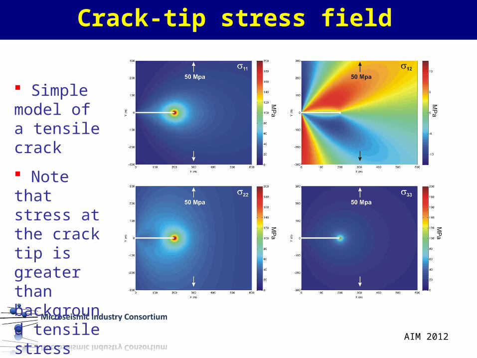
Crack-tip stress field

Simple model of a tensile crack

Note that stress at the crack tip is greater than background tensile stress

15

AIM 2012

is the change in shear stress μ the coefficient of friction n is the normal stress P is the pore fluid pressure

Coulomb Stress Field

A measure of the state of stress on a planar surface.

16

AIM 2012

Coulomb stress changes calculated for the 23 April 1992 ML=6.1 Joshua Tree Earthquake. Aftershocks occur preferentially in areas of increased Coulomb stress

King et al., 1994

Coulomb Stress and Aftershocks

17

AIM 2012

Stochastic Model

20% probability of failure for CFS >= 80 MPa

Magnitude distribution satisfies Gutenberg-Richter relation with b = 1.5

Dynamic simulation created by assuming an expanding crack with c ~ t1/2

18

AIM 2012

Eaton et al., 2011

Detection Threshold

19

AIM 2012

Snapshot from Simulation

20

AIM 2012

In this case study, radiated seismic energy - even after correction for catalog incompleteness - represents only a few ppm of the injection energy

An idealized geodynamical simulation framework has been developed that matches some characteristics of field observations, including diffusion-like event migration and presumed receiver-side observational bias

Conclusions