energy efficiency analysis and optimisation of hipa power

Analysis and Optimisation of HIPA Power Consumption-20161214.docx

1/47

Energy Efficiency Analysis and Optimisation of HIPA Power Consumption

Andras Kovach, Angelina Parfenova

14.12.2016


2/47

Table of Content

1 Introduction ..................................................................................................................................... 3

1.1 Motivation and Aims ........................................................................................................... 3

1.2 Aims .................................................................................................................................... 4

2 Analysis of Electrical Supply Grid..................................................................................................... 4

2.1 General Layout .................................................................................................................... 4

2.2 The central SCADA system: GLS .......................................................................................... 6

2.3 Analysis of Electrical Measurement System ....................................................................... 7

2.4 Summary ........................................................................................................................... 15

3 Power consumption ...................................................................................................................... 16

3.1 List of consumers with classification ................................................................................ 16

3.2 Power during full beam .................................................................................................... 18

3.3 Efficiency of Minimum Full Beam ..................................................................................... 19

3.4 Energy Flow Diagram ........................................................................................................ 20

3.5 Power Consumption of Subs-System ................................................................................ 21

3.6 Comparison of Approaches and Energy Consumption ..................................................... 44

3.7 Summary of Saving Measures ........................................................................................... 46

4 Conclusion and Further Work ....................................................................................................... 47


3/47

1 Introduction

As the world is becoming more energy conscious and environmental issues play an ever increasing role, electrical energy becomes more and more valuable. Therefore, knowing where and how energy is consumed is the first step that can be made along the long path of energy optimisation. At PSI the largest consumer of electrical energy is the HIPA facility by far. Although its power consumption was previously estimated to be approximately 10 MW (without cryogenics), these estimations were never verified by measurements or system-wide power analysis. This study aims at addressing this issue by (1) analysing the electrical grid and the power distribution (2) systematically evaluating on the power consumption of every sub-systems, (3) elaborating on the accelerator’s performance (eg. grid to beam efficiency) and (4) identifying areas of possible energy saving and by suggestion possible improvements.

1.1 Motivation and Aims Due to the increasing global attention to the environmental impact of accelerators, there have been a number of motivating factors to conduct the present study:

EnEfficient (EuCARD-2)

The EuCARD-2 integrated activity project is aimed at coordinated and collaborative R&D on particle accelerators. The EnEfficient network of EuCARD-2 has set the specific goal of addressing accelerator efficiency and cost effective electrical energy utilisation. The study was supported by EnEfficinet as a part of the network’s efforts to gain better understanding of the energy use of high intensity machines with an example on HIPA.

Energy Target 20201 and Energy Strategy 20502

Due to changes in Swiss Federal and Cantonal Energy Law §10, public bodies and institutions are required to increase their energy efficiency as a motivating example for the public sector to pursue similar measures. Being a government funded organisation, PSI is also required to facilitate its electrical resources in a more efficient manner3. An agreement was made on the necessary measures with energy agency EnAW4. PSI is obligated to implement certain measures and thus will be able to apply for refunds of KEV for large research facilities. The analysis of HIPA power consumption is a major step forward in understanding and measuring/estimating the consumption of the facility and in identifying further areas where energy can be saved.

1 https://www.energie-vorbild.admin.ch/vbe/en/home/energieziel_2020/initiativen.html 2 http://www.bfe.admin.ch/energiestrategie2050/index.html?lang=en 3 https://www.energie-vorbild.admin.ch/vbe/en/home/aktionsplaene0/aktionsplaene_akteure/eth.html 4 https://www.enaw.ch/en/

Source: https://www.psi.ch/enefficient/SCHeaderEN/eucard2_logo.jpg

https://www.energie-vorbild.admin.ch/vbe/en/home/energieziel_2020/initiativen.html

http://www.bfe.admin.ch/energiestrategie2050/index.html?lang=en

https://www.energie-vorbild.admin.ch/vbe/en/home/aktionsplaene0/aktionsplaene_akteure/eth.html

https://www.enaw.ch/en/


4/47

PSI Energy Concept5

PSI puts large emphasis on its environmental impact and the highly efficient utilisation of its resources and facilities. The values outlined in the guiding principles of the PSI Environmental Concept6 have also supported the realisation of this study.

1.2 Aims The study had the following initial aims:

• Establish a list of power consumers

• Classify consumers

• Find power consumption of sub-systems and their dependency on beam power, season, etc.

• Analyse structure of electrical grid

• Identify possible improvements

2 Analysis of Electrical Supply Grid

2.1 General Layout PSI connects directly to the Axpo 50/110 kV public grid. As of 2016 the grid voltage is 50 kV, however, a transition to 110 kV will be made in 2017. At a local sub-station this voltage is stepped down to a middle voltage of 16 kV. There are two such high voltage transformers installed for redundancy reasons. The 16 kV middle voltage is used to distribute power over the east and west sides of PSI. Low voltage (400 V) is achieved in the last step of transformation, usually in the close proximity of the end-user. In principle all of the 16 kV to 400 V transformers are dedicated to supply a specific consumer.

5 https://www.psi.ch/about/psi-energy-concept 6 https://www.psi.ch/about/psi-environmental-concept


5/47

Figure 1: Layout of electrical grid at PSI. (source: PSI, 2010)

Figure 2 shows the 16 KV HIPA supply ring ‘Ring WBGA’ that provides power to the 400V transformers. This ring is connected to the 16 kV PSI line though two switchgears (also for redundancy): T3-A17 and T3-A26. Both the high and low voltage sides of the 400 V transformers are equipped with switchgears.

Figure 2: The layout of HIPA supply ring ‘Ring WBGA‘. See source document in Appendix XXX.


6/47

Despite the neatly designed layout, the HIPA supply ring also delivers power to areas which are not relevant to the HIPA facility. These additional facilities and their respective transformers are:

• Transformer K1-T1: The SULTAN facility • Transformer WLHA–T1: SwissFEL test area • Transformer E1-m1: Offices (not HIPA-relevant) and

groundwater pumps (partially HIPA- relevant)

Transformers G1-T1 and G1-T2 also supply HIPA, more specifically the Injector 2 RF components; however, they are not connected to the HIPA ring, but to the general 16 kV PSI line.

The low voltage side of the transformers feed through a meter and then to an electric control cabinet. These cabinets are used to spread out the electrical supply voltage to power consumers in an organised and structured manner. Main consumers are labelled on the slots of the cabinets, while smaller consumers (without having a separate slot) are registered on a list. Full list is available from Emanuel Hüsler on request.

Although theoretically separate, it was also found that certain transformers (and power cabinets) supply multiple sub-systems of HIPA simultaneously. This, however, is inevitably inherent to the system because a) HIPA is an old machine and modifications were continuously were made to it and b) doing the cabling for a certain area twice just to have fully separated power suppliers is financially not viable. The cases when such mixing happens are evaluated in the next section.

HIPA has four major power distribution sites, where sets of power cabinets are located. These sites can be found in/on:

• The WSGA building • West gallery 2 in WEHA • East gallery 2 in WEHA • Gallery 2 WNHA

2.2 The central SCADA system: GLS GLS (Gebäudeleitsystem) is a SCADA (Supervisory Control and Data Acquisition) system at PSI used for controlling, monitoring, alarming and archiving parameters of the facilities and the infrastructure. GLS provides a high-level control system and process supervisory management, featuring thousands of measurements points. When equipped with the appropriate module, electrical meters can be connected to GLS and their measurement values can be monitored and archived. Archiving gives access to years of historic data, which proves to be extremely useful when analysing the performance or power consumption of the facility.

Data stored in GLS can be accessed through the java-based application ‘Egli-tool - GLS Visualisierung und Reporting’ version 2.5.2. Advantages of this tool include: searching all measurement points,

Figure 3: Power cabinet with power breaker, multi-measurement devices and

distribution slots.


7/47

creating and storing private list and exporting private list to csv file. However, a search can only be performed for the Description field and not the name of a measurement point. Furthermore it can only be accessed with remote desktop connection and the speed of the application is considered rather slow by today’s standards.

Having realised its limitations and the hugely advanced energy monitoring and visualisation capabilities of modern software, the Egli-tool is being replaced with e3m, an Active Energy Data Management software provided by SILENO AG. The e3m environment has tools for displaying statistical data about consumption, power needs The present study urges the integration of e3m with GLS as it can provide a level of insight into PSI’s energy needs that was previously not possible.

2.3 Analysis of Electrical Measurement System

Figure 4: The GLS Visualisierung und Reporting java application

Within the HIPA supply ring, electrical meters are installed at the two middle voltage switchgears as well as on the low voltage side of most 400 V transformers. The meters in the latter case are Socomec DIRIS A40 multi-measurement meters, which are capable of measuring, I, U, PF, P, Q and S for every phase with an accuracy of 0.5% along with kWh energy consumption with an accuracy no worse than 2.5% (ref to datasheet). With an additional communications module, these data feeds of the meters can be connected to the GLS through RS485 serial or RJ45 Ethernet interface.

Most of the DIRIS meters are also equipped with a communication module, although there are exceptions. The following section will evaluate on the metering of every transformer (as listed in )and will also aim to assess whether the installation of additional meters is recommended.


8/47

Transformer Meter Location In GLS Main Consumer

S1-T15 S5.2 Yes Water cooling S1-T14 S6.17 Yes Ring + Inj2 magnets S1-T13 S82.13 Yes Ring RF pre-amps S1-T12 S6.1 Yes P-Kanal + Extraction S1-T11 S5.19 Yes UCN S1-T10 No Meter No Rectifier 5 S3-T7 No Meter No Rectifier 4 S3-T6 No Meter No Rectifier 3 S3-T5 No Meter No Rectifier 2 S3-T4 No Meter No Rectifier 1 E2-T1 E2.31 Yes PiM3 E2-T2 E2.41 Yes PiE5 E2-T3 E2.1 Yes PiM1 WLHA-T1 A01.007.01 Yes SwissFEL test facility E1-M1 E1.11 Yes PiE1 and MuE4 B1-M2 B3.2 ? offices and groundwater

KS3-T2 ? Yes Compressor 2 (KA1 SINQ)

KS3-T1 ? Yes Comressor 1 (KA4) K1-T1 ? Yes Sultan NH-T2 NH2.13.21 Yes SINQ Infrastructure NH-T1 NH2.12.21 Yes SINQ magnets E1-T2 E1.60 Yes Infrastructure E1-T1 E1.50 Yes MuE1 and PiE3 G1-T1 G60.1&G60.20 Yes Inj2 machine + generic G1-T2 ? Yes 15kV rectifier

Table 1: List of transformers within the HIPA supply ring. G1-T1 and G1-T2 are additional HIPA-relevant transformers connected directly to the 16 kV PSI line.

S1-T15 (Hausbedarf (Cooling), meter location S5.2)

The main consumer of the S1-T15 transformer is the water cooling centre in the WSGA building. During Normal operation, the consumption is roughly 900 kW (S5.2) out of which 650 kW goes to the cooling centre (S5.2). The remaining ~250 kW is used by smaller consumers, out of which the secondary cooling circuits KK6.6 and 6.7 account for approximately 150 kW.


9/47

Figure 5: Simplified schematic drawing for S1-T15 transformer energy flow.

As shown in Figure 5, only the S5.2 meter is available in GLS. Although a meter is installed for the cooling centre branch it is not connected to GLS. Therefore the consumption value on S5.1 was manually recorded 4 times in October 2016. During beam operation 640-650 kW was recorded (3 measurements) and during service 560 kW was measured (1 measurement).

As a result of the present investigation it was found that despite the meter displaying the correct power consumption value, the kW measurement in GLS was a factor of 10 less than on the meter. The meter and the communications module were both replaced. As a result the measurement point in GLS became a valid value.

Recommended measures:

• Connecting the S5.1 meter to GLS would provide better information about the power consumption of the cooling centre (dependency on beam power, season and mode of beam operation).

• It would also be advised to meter KK6.6 and 6.7 as they are also major consumers of electrical power for cooling.

• Analyse and categorise the rest of the consumer with typical consumption values.

S1-T14 (Ring + Injector; meter location S6.17)


The S1-T14 transformer supplies the coils of the sector magnets as well as magnets along in the Ring and in Injector 2. Despite the installed mater at S6.18, the energy consumption of the sector magnet coils is not available in GLS. The consumption value on S6.18 was recorded manually 4 times in October 2016. In every occasion a load 657 kW was recorded.


• Connecting the S6.18 meter to GLS would provide better information about the power consumption of the cooling centre.

• Verify that power from S6.17 only goes to magnets. Once verified, the difference between S6.17 and S6.18 can provide useful information about the energy consumption of magnets.


10/47

S1-T13 (RF Pre-amplifiers; meter location S82.13)

The S1-T13 transformer provides power for the first stages of RF amplifiers in the Ring cyclotron. This transformer is well separated and has a dedicated function. Furthermore, the Measurement of the S82.13 meter is available in GLS.

S1-T12 (P-channel and Extraction; meter location S6.1)

Magnets and instruments along the P-channel and in the extraction are mostly supplied by the S1-T12 transformer. At an early stage of the investigation, it was found that the DIRIS meter displays -20 W for the real power, while having ca 1 MW of apparent power. This was clearly a fault and hence was further investigated. After connecting a portable meter and monitoring for a few weeks it was found that the 3 phase probes of the meter were misconfigured. Misconfigured data was fed to GLS since the beginning of 2015 as shown in Figure 7. The fault was corrected and it was verified that real power values are correct on the meter as well as in GLS.

Figure 7: Plot of archived data (from January 2013 to October 2016) for real power, apparent power

and Power Factor for meter S6.1.

S1-T11 (UCN; meter location S5.19)

The S1-T11 transformer is dedicated to the UCN beamline and experiment area. It also supplies power to the KA2 Helium compressor of the UCN cryo-cooling system. The consumption of the transformer is measured on the meter at S5.19. There are two additional meters on S5.20 and S5.20 which measure the lines running to UCN experiment area and the Helium compressor, respectively. The difference between the S.19 meter and the sum of S5.20 and S5.21 is the power taken up by the UCN magnets.


11/47



• Connect the S5.20 and S5.21 to GLS so that energy consumption of the KA2 helium compressor and UCN experiment areas can be monitored.

• Verify that the remaining consumers are only UCN magnets

S1-T10, 7, 6, 5, 4 (RF)

These transformers provide power to the 16 kV rectifiers and RF amplifier chains of the Ring machine. Overall they take up to 4 MW at a high beam current operation (for details see section XXX). Despite being one of the major power consumers, there are no meters installed and hence their power consumption can only be manually measured.

The first point when RF power is monitored is in front of the cavities. By that point approximately 50% of the invested grid power is lost. Although the grid to RF power ratio is known to be 0.5 as a rule of thumbs, it is highly recommended to install meters to each one of these transformers. Knowing the power consumption of the RF components more accurately would make the optimisation of RF easier. Furthermore, it would serve also as a continuous feedback and would hugely increase the accuracy of energy metering for HIPA.

As discussed with Markus Schneider, the control system for the Ring amplifiers is planned to be modernised after the Injector 2 upgrade (earliest 2020). This modernisation will enable the RF group to easily set operation points for amplifiers and it will also include the installation of electrical measurement points.

For the purpose of more accurate energy monitoring the installation of electrical meters could also be justified at an earlier stage.


12/47

E2-T1 (PiM3), E2-T2 (PiE5) and E2-T3 (PiM1)

The E2-T1 (PiM3), E2-T2 (PiE5) and E2-T3 (PiM1) transformers have active metering at locations E2.31, E3.41 and E2.1, respectively. The values of these meters are also available in GLS. The main consumers were assumed to be the beamline magnets, however, it was found that beamlines magnet account for no more than 2/3 of the total power consumption values (for details see Section XXX).

Add comparison of measurement and calculation. Done in section 3.5.1.4

A list of all consumers (Legende) is available from René Räch. This list also indicates the value of installed fuse for every consumer. It is advised to manually measuring those loads, which have large fuses, and hence identify and classify these smaller power consumers.

WLHA-T1 (SwissFEL test facility)

This transformer provides electricity to the WLHA building, where the SwissFEL test facility is located. There is a meter installed at A01.007.01 and it is available in GLS, however, it is not the part of HIPA and hence it was not examined in the present study.

E1-m1 (PiE1 and MuE4; meter location E1.11)

The PiE1 and MuE4 beamlines are powered from the E1-m1 transformer. There are two meters in this system. One meter is installed at the entry point to the power distribution cabinet and another one where MuE4 branches off. As Figure 9 shows, the difference between E1.11 andE1.12 yields the consumption of PiE1.

A single manual measurement was made on 24.11.2016 to compare the power consumption of the beamline based the current through the magnets with the power value displayed on the meter. It has revealed that while the E1.12 meter showed 153 kW, the magnets could only account for 88 kW.

Figure 9: Simplified schematic drawing for E1-m1 transformer energy flow.


• Connect the E1.12 meter to GLS to be able to monitor the consumption of MuE4 • Identify and classify smaller consumers (loads apart from magnets)


13/47

B1-M2 (offices and groundwater; meter location B3.2)

The B3.2 area is a special one, because - besides supplying power for offices and for the groundwater pumps – it also provides the emergency supplies with power. In case of a power cut, the supply to the emergency section from B1-M2 stops, the generators kick is and after a short pause, elements of the emergency circuit regain power. The B3.2 meter is connected to GLS


• Separate out ground water supply and add to GLS (to be verified)

KS3-T2 (Compressor 2 (KA1 SINQ)) and KS3-T1 (Compressor 1 (KA4)

Theses transformers supply the Helium compressors of the KA1 and KA2 cryo cooling machines. Both are monitored on the low 400 V side the measurement points are available in GLS. KS3-T1 supplies Compressor 1 (KA4) exclusively; however, KS3-T2 also delivers power to magnet power supplies for the Sultan experiment. Therefore it is advised to add at least one meter to separate the HIPA-relevant power from non-relevant power. Not only would it help to monitor HIPA’s power more precisely, but also to assess the Sultan experiment’s energy use more accurately.

K1-T1 (Sultan)

The energy consumption of the Sultan experiment is provided from the HIPA supply ring. Its consumption is metered and also connected to GLS since January 2016, however, it is not the part of HIPA facility and hence it was not examined in the present study.

NH-T2 (SINQ Infrastructure; meter location NH2.13.21)

The meter at location NH2.13.21 measures the energy taken from transformer NH-T2. This power is used for supplying the SINQ infrastructure. One of its main consumers is the SINQ water cooling system, which accounts for approximately 100 kW of continuous load. The remaining 100 kW is consumed by other infrastructure.

It is recommended to identify where the remaining 100 kW of power goes within SINQ.

NH-T1 (SINQ Magnets; meter location NH2.13.21)

The NH-T1 transformer principally supplies the magnets of the SINQ beamline. When in operation it results in a load of ca. 560 kW. In 2016 SINQ had a long outage, when magnets of the beamline were switched to Standby through the SLEEP control software. During this period the meter has only indicated a power consumption of 11 kW. This shows that magnets are very well separated for SINQ on the NH-T1 transformer.

E1-T2 (Infrastructure; meter location E1.60)

Most parts of the HIPA infrastructure are supplied from the transformer E1-T2. The meter in the WEHA building on the West Gallery 2 at E1.60 measures the energy taken from the transformer. This line goes up to Gallery 3, where the distribution units are located for the infrastructure. The main consumers of this power are ventilation and lighting. Smaller consumers are air conditioning,


14/47

heating, control systems, etc. The power consumption of HIPA infrastructure is studied in detail in Section3.5.

E1-T1 (MuE1 and PiE3; meter location E1.50)

The study has revealed that the E1-T1 transformer not only supplies MuE1, but also the PiE3 beamline. The transformer has a typical consumption of 600 kW, out of which MuE1 magnets consume up to 300 kW and PiE3 magnets consume ? kW. The difference of the remaining power was investigated and it was found that some magnets along the P-channel are also supplied from E1.50. These magnets contribute with an additional 200 kW to the power consumption. The remaining difference is advised to be investigated and allocated to relevant sub-systems.

G1-T1 (Injector 2 machine + generic) and G1-T2 (Injector 2 15 kV rectifier)

These two transformers feed the Injector 2 machine and the surrounding devices and instruments with electricity. G1-T2 is monitored at the high side switchgear. For G1-T1 there is a high side monitor as well as two low side monitors G60.20 and G60.01 in parallel configuration. After the low side monitors there are two sub-consumers monitored: G60.29 (Hausbedarf/Infrastructure) and G60.12 (Notenetz/Emergency power), both available in GLS. However, the complex layout of Injector 2’s RF system makes power measurement and monitoring of specific sub-systems extremely challenging. The Resonator upgrade (starting in 2018) will also aim at simplifying the RF supply system and it will incorporate measurement points.

Figure 10: Simplified schematic drawing for transformers G1-T1 and G1-T2 energy flow.


15/47

It was also found that the cooling circuit 2Cu (cooling of Ring cavities) is supplied by the G1-T1 transformer. Adding a separate meter to the 2Cu cooling circuit would be beneficial for accurately measuring and optimising the cooling needs of HIPA.

2.4 Summary The above results show that HIPA has a well-structured electrical supply grid in general. In every case power distribution cabinets and their sub-consumers are well documented. Metering is implemented in many cases; however, the meters are only connected to the central SCADA system (GLS) to a limited extent. Connecting these meters to GLS would increase the understanding of HIPA’s energy consumption.

The analysis has also highlighted that certain transformers cannot be fully allocated to a specific sub-consumer. The list Table 1 summarises the areas where the introduction of additional electrical multi-meters (with access to GLS) would be of great benefit for the facility. When the large number of sub-consumers (or their relatively low power consumption) does not justify the addition of a fixed meter device, it is still advised to confirm and categorise their power consumption values. During the study two faulty/misconfigured meters have been identified (ca. 1.6 MW incorrectly measured). With the systematic verification (and classification) of sub-consumers of power distribution cabinets, such faults could be minimised.

Table 2: Suggested new emeltrical meter locations

The only area where power monitoring is missing entirely is the supply chain for the Ring RF components. Since these transformers account for a significant ca 4 MW power, it is strongly advised to introduce power monitoring, regardless of the planned amplifier control system upgrade (earlies start in 2020).

The replacement of the outdated GLS data retrieval java application (Egli-tool - GLS Visualisierung und Reporting) is a most welcome step; and the configuration of the new e3m web interface is

The not fully implemented monitoring system and the fact that transformers tend to supply multiple sub-systems of HIPA has limited the applicability of a top to bottom analysis approach. Therefore the following sections break down the facility’s power consumption using a bottom-up approach. However, where applicable, the two approaches are compared.

Add meter Connect to GLSS5.1 to cooling centre - Yessub S5.3 KK6.6&6.7 Yes YesS6.18 sector magnets - YesS5.21 He compressor KA2 - YesS5.20 UCN exp. Area - YesS1-T10, 7, 6, 5, 4 RF tansformers Yes YesE1.12 MuE4 - Yessub B3.2 separate out groudnwater ? Yessub KS3-T2 separate out He KA and Slut Yes Yes

ActionLocation Description


16/47

3 Power consumption

This section presents the power consumption value for the facility, lists and categorises the sub-systems, describes and analyses the consumption of these consumers, suggests potential saving measures and presents a grid to beam efficiency for a minimum full beam setup.

3.1 List of consumers with classification In order to analyse the distribution of the facility’s power consumption, it was found vital to create a comprehensive list of all power consumers. When creating the list found in Table 3, the bottom up approach was taken to ensure that the consumption values allocated to the categories are as accurate as possible. Despite the clear list of consumers, their classification was found to be ambiguous, and therefore it is vital to precisely define the categories and their scopes. Consumers were classified into the following categories:

• Accelerator: Includes all consumers, which are minimally required for the production of a full beam at the extraction from the Ring. By defining this category, the performance of the HIPA machine can be evaluated without taking into account the remaining parts of the facility. This evaluation has high scientific usefulness and it is detailed in Section 19

• Water Cooling: Includes every consumer related to the cooling of the machine, magnets, experiments and other components.

• Infrastructure: This category includes all consumers which are related to the HIPA buildings and the experiment halls. Systems are considered as infrastructure if their function is to provide the space and the controlled environmental factors to operate the facility.

• Auxiliary: Those essential parts of the machine and the facility, which do not form part of the accelerator itself, but are vital for transporting the beam and for providing the experiment sites.

Table 3 shows the list of consumers, their classification and their power consumption under full load at the production of a 2.2 mA beam.


17/47

Table 3: HIPA sub-systems, their classification and power consumption

The Cockcroft-Walton pre-accelerator, all RF components and sector magnets are classified as Accelerator for obvious reasons. Primary beamline magnets, however, are only partially considered Accelerator (20%), as most of the magnets are located after the extraction from the Ring. The 20% value was allocated to Accelerator after measuring the power consumption of every magnet of the beamline. All secondary beamlines belong to Auxiliary systems, because they are not part of the accelerator machine. Water cooling partially belongs to Accelerator, since parts of the machine (RF, magnets between Injector 2 and the Ring, etc.) require cooling. This shared allocation is an example of how one sub-system can be part of more than one categories. Cryogenics are also classified as part of Auxiliary systems. The category Infrastructure consists of already known and measured consumers such as lighting, air conditioning and ventilation. Other consumers of Infrastructure power are heating, power plugs throughout the experiment halls control systems etc. Every sub-consumer of the facility is evaluated to greater extent in later sections of the study.


18/47

3.2 Power during full beam The previous table has also revealed the power consumption of every sub-system as well as the total 12.5 MW power consumption of the facility. At a full load HIPA accounts for more than the half of PSI’s ca 20 MW of total power consumption. It shall be emphasised that reaching the consumption of 12.5 MW requires all experiment areas (IP2, UCN, SINQ and all secondary beamline experiments) to run simultaneously.

Figure 11: Distribution of HIPA power under full load at 2.2 mA beam

RF is the single largest power consumer with 42% of all HIPA power. The input 5.3 MW power is transmitted to the beam in Injector 2 (ca 900 kW) and in the Ring (4.4 MW) to achieve a final beam power of 1.3 MW. About half of the 5.3 MW grid power is lost in the amplification step (creating RF power) and a second half is lost when transmitting power to the beam. Sector magnets are also essential parts of the cyclotrons and they consume 657 kW or 5%. The power consumption of the primary beamline magnets was measured to be 2.3 MW. The largest portion of this is needed by high power bending magnets. Water cooling is an unexpectedly high power consumer with ca 1.7 MW, which is approximately 10 times its cooling. Cryogenics is a steady and continuous load due to the nature of cyro-cooling machines.

The method for measuring the power consumption of sub-systems was dependent on the characteristics of the system, therefore no unified can be made about the accuracy of the above numbers. In most cases however, the consumption for sub-systems was obtained by adding up numerous smaller measurements, which on average had no more than 5-10% error. Given the large number of these small measurements, it is expected to average out and hence the 12.5 MW value is correct to 5%.


19/47

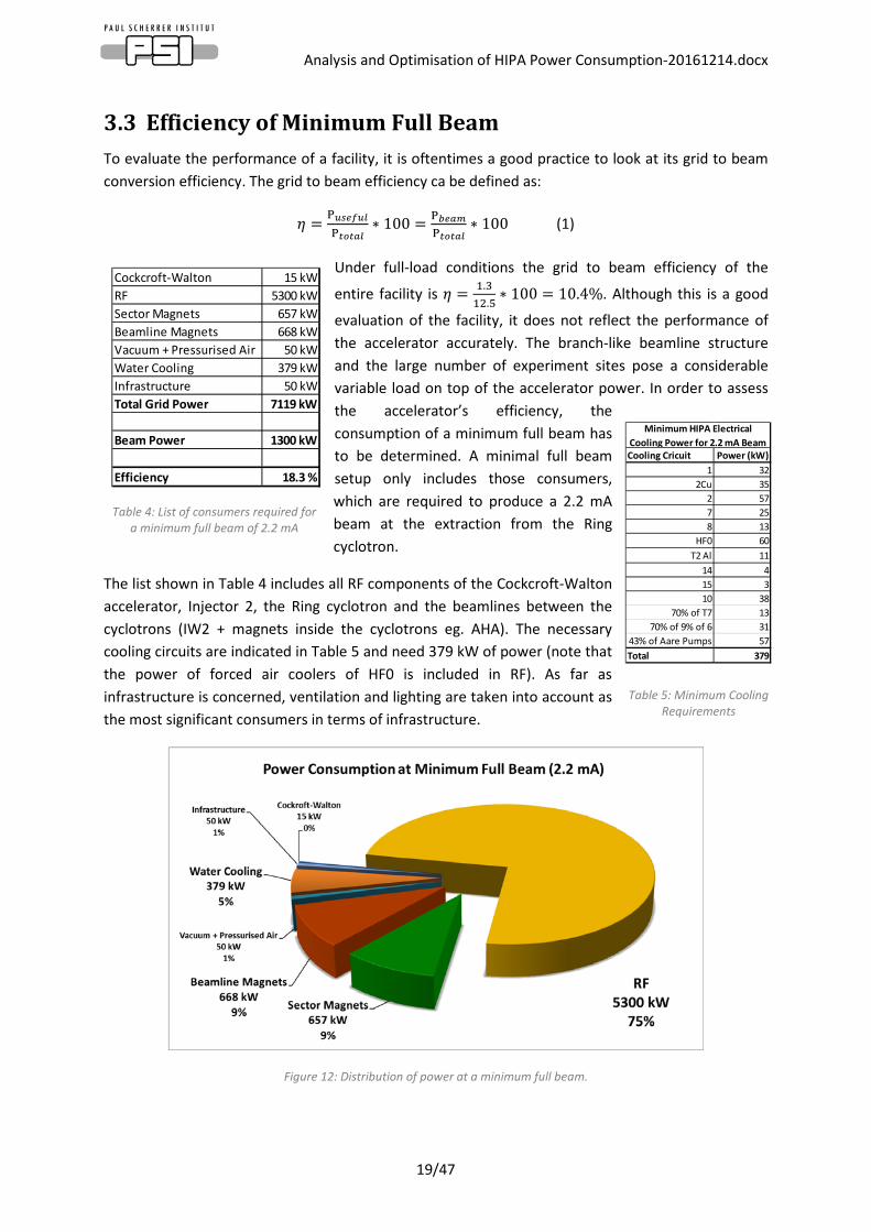
3.3 Efficiency of Minimum Full Beam To evaluate the performance of a facility, it is oftentimes a good practice to look at its grid to beam conversion efficiency. The grid to beam efficiency ca be defined as:

𝜂𝜂 = P𝑢𝑢𝑢𝑢𝑢𝑢𝑢𝑢𝑢𝑢𝑢𝑢P𝑡𝑡𝑡𝑡𝑡𝑡𝑡𝑡𝑢𝑢

∗ 100 = P𝑏𝑏𝑢𝑢𝑡𝑡𝑏𝑏P𝑡𝑡𝑡𝑡𝑡𝑡𝑡𝑡𝑢𝑢

∗ 100 (1)

Under full-load conditions the grid to beam efficiency of the

entire facility is 𝜂𝜂 = 1.312.5

∗ 100 = 10.4%. Although this is a good

evaluation of the facility, it does not reflect the performance of the accelerator accurately. The branch-like beamline structure and the large number of experiment sites pose a considerable variable load on top of the accelerator power. In order to assess the accelerator’s efficiency, the consumption of a minimum full beam has to be determined. A minimal full beam setup only includes those consumers, which are required to produce a 2.2 mA beam at the extraction from the Ring cyclotron.

The list shown in Table 4 includes all RF components of the Cockcroft-Walton accelerator, Injector 2, the Ring cyclotron and the beamlines between the cyclotrons (IW2 + magnets inside the cyclotrons eg. AHA). The necessary cooling circuits are indicated in Table 5 and need 379 kW of power (note that the power of forced air coolers of HF0 is included in RF). As far as infrastructure is concerned, ventilation and lighting are taken into account as the most significant consumers in terms of infrastructure.

Figure 12: Distribution of power at a minimum full beam.

Table 4: List of consumers required for a minimum full beam of 2.2 mA

Cooling Cricuit Power (kW)1 32

2Cu 352 577 258 13

HF0 60T2 Al 11

14 415 310 38

70% of T7 1370% of 9% of 6 31

43% of Aare Pumps 57Total 379

Minimum HIPA Electrical Cooling Power for 2.2 mA Beam

Cockcroft-Walton 15 kWRF 5300 kWSector Magnets 657 kWBeamline Magnets 668 kWVacuum + Pressurised Air 50 kWWater Cooling 379 kWInfrastructure 50 kWTotal Grid Power 7119 kW

Beam Power 1300 kW

Efficiency 18.3 %

Table 5: Minimum Cooling Requirements


20/47

Hence the minimum power consumption for a full beam is 7.12 MW. This in turn yields a gird to

beam efficiency of 𝜂𝜂 = 1.37.12

∗ 100 = 18.3 %. The 7.12 MW requirements and the 18.3 % efficiency

can be used as the most accurate measurement on HIPA’s performance so far. Furthermore, it can be a good reference value in the design of ADS systems.

The RF systems’ power needs are linearly dependant on the beam power in this region of operation. Most of the remaining sub-systems show very little or no dependency on the power of the produced beam. Therefore the load of 1.8 MW can be considered as a base load and the RF as a beam dependent load. Hence the system’s efficiency could be further increased by increasing the beam power.

(Note that the accelerator’s efficiency was previously estimated to be 18 % at a 1.4 MW (2.4 mA) beam and consumption of 8 MW. If the measurements of the present calculation are projected to a 1.4 MW beam, then the expected consumption is 7.4 MW (increase in RF consumption) and the efficiency would be ca. 19 %.)

3.4 Energy Flow Diagram

Figure 13: HIPA energy flow diagram

The diagram below was created to demonstrate how grid power is converted to beam power. The largest consumer RF contributes directly towards transferring power to the beam, however, auxiliary systems and magnets also play and essential role and contribute to the beam indirectly.

A second energy flow diagram (Figure 14a) was created to be comparable with the existing (and already published) energy flow diagram (Figure 14b) of the facility. For the purpose of comparability, the power required by cryogenics was deduced from the 12.5 MW total, hence yielding 11.3 MW. This is 1.3 MW more than previously anticipated.


21/47

Figure 14 a) the ‘old‘ HIPA energy flow diagram b) the new HIPA energy flow diagram.

The major source for this difference is the power taken up by the RF systems. In the present study the gird power of the Ring’s RF system was measured to be 4.4 MW and the Injector 2 power was estimated to be 900 kW, adding up to the total of 5.3 MW. This difference explains5.3 MW – 4.1 MW = 1.2 MW out of the 1.4 MW difference.

Furthermore, the sector magnets, the primary and secondary beamline magnets were measured to consume 656 kW, 2300 kW and 675 KW, respectively, thus a total of 3.6 MW. This is exactly 1 MW more than previously assessed.

In terms of auxiliary systems the consumption is less than expected by 800 kW. One of the reasons for the higher value in magnet power and lower value in auxiliary system could be that magnets were partially counted towards auxiliary systems. The difference between the total sums of ‘Magnets’ and ‘Auxiliary’ accounts for the remaining 200 kW difference between the old and the new measurements.

3.5 Power Consumption of Subs-System This section will detail the power consumption of every sub-system of HIPA. It also aims at describing the source of data, the measurement methods used and any influencing factors on consumption such as season or beam intensity. Where applicable, the saving potential is also identified and estimated. Limitations of the study and/or measurements are also outlined.

3.5.1.1 RF

The most significant consumer of HIPA is the RF system. Injector 2 and the Ring machine have their own amplifier chains for every cavity and resonator. Cavities (1-5) in the Ring are supplied by transformers (S3-T4, T5, T6, R7 and S1-T11, T13) and rectifiers (Gleichschalteranlage 1-5). Elements of Injector 2 are power from transformers G1-T1 and T2. The eclectrical spuuly system for Rf components is detailed in Section 2.3.

During the analysis process the power consumption of the Ring machine was studied in detail and exact power consumption values were only obtained for the Ring. Injector 2 was not studied to the same detail for several reasons 1) the supply chain for Injector 2 is more complex and any measurements would be more time consuming 2) Injector 2 will undergo an upgrade starting in the long shutdown of 2018 3)the larger RF consumer had priority due to time constraints of the study.


22/47

Therefore, for Injector 2 it was assumed that the grid to beam efficiency is 50%. The following parts of the RF evaluation were made on the Ring, however, the principles also apply to Injector 2.

Figure 15: RF system energy flow

Figure 15 depicts the stages of energy conversion from the grid to the beam. Every cavity (1-4) of the Ring has such an amplification chain. The first stage is an AC-DC rectification, with an efficiency of ca. 90%. Then the DC voltage is fed to the amplifier chain (Figure 16) where RF power is produced. This stage facilitates a chain of amplifiers with tetrode tubes. The combination of all amplifications stages has an approximate efficiency of 60%. From the amplifiers, the high frequency signal travels through a high power transmission line, where it encounters Ploss transmission. After entering the cavity, a part of the RF forward power will be transferred to the beam. This Pbeam is considered as the useful work when assessing the efficiency of the accelerator/facility. The major part of the remaining RF forward power dissipates in form of wall losses (Ploss wall). Ploss reflected the portion of RF forward power that gets reflected form the cavity/resonator, travels through the transmission line again and also dissipates upon reaching the amplifier.

When the RF system was designed, power monitoring and energy efficiency was not considered as high priority. Thus the system lacks digital electrical measurement points. Measurements can be manually made on the AC middle voltage at point D. This can be considered as the grid power consumed. Besides many other parameters, the power can be measured before (rectified DC) and after the amplification stages (RF forward power) at points E and A. These are also manual measurements. The First readily-available power measurement is made on the RF forward before it enters the cavity at point B. This measurement is available in EPICS, with the channel pattern CR1IN:IST:2 as an example for Cavity 1. These channels are also archived. The Reflected power is also available in EPICS; but for an energy analysis study those values do not convey significant value.

Figure 16: Tetrode Tube Amplifier Chain. Courtesy of M. Schneider.


23/47

The fact that most steps of the RF energy conversion do not monitor power, makes system evaluation rather challenging. Historically, only very limited or no exact data was available about RF power consumption. M. Schneider has recently performed measurements at no beam, 1.2 mA beam and 2.4 mA beam. During these measurements the configurations of the Cavities were not changed (same gap voltage).

Table 6: Conversion efficiency of RF stages at 2.4 mA beam.

Detailed data of the power measurements for each cavity is available in Appendix A. The efficiency of energy conversion between stages is summarised in Table 6. The efficiencies were calculated based on measurements at a 2.4 mA beam. From the data indicated in Appendix A, it would seem that RF efficiency varies with the produced RF power. However, the RF settings for the measurements were optimised for a 2.4 mA beam. If RF was optimised for every beam current specifically, similar efficiency values would be expected. Therefore the table above can be used as a rule of thumbs for other beam powers too. It shall also be noted that these numbers were obtained based on a single measurement.

Table 7: RF system efficiency. Data courtesy of M. Schneider

Examining the dependency of the RF system (as a whole) on beam power can directly reveal more useful data about the system’s characteristics. As shown in Table 7, the grid to RF efficiency is 55% at 2.4 mA beam and it gradually reduces as the beam current decreases. If optimised, this efficiency would stay close to 55% at lower beam currents as well.

Efficiency (%)Grid → DC 90DC→ RF 65RF → Beam 55

Beam current (mA) 0 1.19 2.4

Forward RF powercavity 1 (kW) 225 440 649cavity 2 (kW) 250 415 620cavity 3 (kW) 280 440 640cavity 4 (kW) 265 440 625Flattop cavity (kW) 110 87 14Total forward RF power (kW) 1130 1822 2548

Grid powerAnode PS 1 (kW) 413 739 1002Anode PS 2 (kW) 413 718 995Anode PS 3 (kW) 456 775 1052Anode PS 4 (kW) 435 754 1016Power distibution WSGA (kW) 526 535 533Total Grid Power (kW) 2244 3522 4599

Efficiency (%) 50 52 55


24/47

Figure 17: Ring cyclotron RF system power consumption. Data courtesy of M. Schneider

Figure 17 demonstrated the linear relationship between the grid power and the produced RF power. At 0 mA beam it can be observed that the system still has a minimum consumption of ca 2.2 MW (from grid). This ‘base load’ power is required for running the system at its operational point and to keep it ready for producing RF power. The control system is design such that the required forward power is automatically adjusted according to the detected beam current. When the beam trips or gets interrupted, power is automatically reduced.

Since the forward power is measured (and archived) in front of the cavities, past data was analysed and plotted for discrete beam currents on Figure 18. It confirms the findings of the previous graph and shows the same linear relationship with more data points.

Figure 18: Ring RF forward power against beam current

The same linear relationship was observed on the RF system of Injector 2 as illustrated on Figure 19.


25/47

Figure 19: Injector 2 RF forward power against beam current

Saving Potential

Summarises the possible energy saving measures and categorises them based to their overall feasibility.

Table 8: List of possible RF energy saving measures

The saving potential of points 1 and 2 was calculated based on historic data analysis with a Matlab script. The program took data downloaded from the archiver and processed it to find a) undocumented and b) additional saving potential.

Table 9: Results of Matlab script for finding saving potential of RF cavities

No. Action Effort Risk Cost Saving Potential Feasibility Comment

1

Setting Ring cavities to a 'Heiz-On' mode when there is no beam for more than 0.5h/2h. Can be implemented by integrating a '30 minute' notification into SLEEP and logic for measuring energy saving.

low low low (<100 kCHF)1086 + 338 MWh/year @ 30 min or 1086 + 210 MWh/year @ 2h

high Assuming grid to RF power efficiency of 50%

2

Setting Injector 2 Resonators to a 'Heiz-On' mode when there is no beam for more than 5 hours. Can be implemented by integrating a '30 minute' notification into SLEEP and logic for measuring energy saving.

low low low (<100 kCHF) 192 + 32 MWh/year highIt takes 2-3 hours for the resonators to satbilitse after they were drive low. During these 2-3 hours the contunuous attention of an operator is required and beam availability could be reduced.

3 Improving AC/DC efficiency (90% to 96%) high low high (>1 MCHF) 1600 MWh/year lowAssuming constatnt 90% conversion efficiency, and 4 MW continuous DC load for 8 months. SLS operational value of 96% still needs to be double checked

4 New Inj2 2&4 Al resonators highAlready planned (2018-2020). Advantages: higher beam current or lower average gap voltage, higher AC/DC conversion efficiency, easier monitoring

5Include Inj2 amplifiers to heat recovery and district heating system

high low high (>1 MCHF) ? medium

The new design incorporates the possibilty of adding cooling circuits to heat recovery system, however, it is not planned ot ne done at the moment. The saving potential could be theoretically calculated (separate task).

6 Upgrading tramsofromers for Ring CavitiesOngoing upgrade, planned 1 transformer/year, slight increase in efficiency (max 1%)

7Look-up table with fixed operationg values for RF amplifier optimisation

medium medium medium200kW reduction after

optimisationmedium Planned after Inj2 upgrade (→earliest 2020)

8Replacing tetrode amplifiers with solid state amplifiers

high high high (>1 MCHF) - lowThe technology is not advanced enough yet and the 50MHz frequncy is not optimal for using solid state drive

9New Cu flattop cavity (preliminary study by N. Pouge)

high low high (>1 MCHF) A feasibility study has to be conducted

10 New Cu resonators for Inj 2 high medium high (>1 MCHF) 576 MWh/year lowAssuming 100 kW reduction of continuous load for 8 months. High CAPEX as cooling circuit also has to be replaced.

11 New cavity desing with optimised shape high medium high (>1 MCHF) high lowLukas Stingeling believes that up 5% could be achieved with fine tunig the shape of the cavities. Note high effort and cost, very long implementation time.

Year Undocumented Saving (MWh) Additional Savings Potential (MWh)2015 818 3462014 1069 3692013 1371 297

Average 1086 338

Ring

Ca

vitie

s


26/47

Undocumented saving potential comes by finding those times when there was no beam and the cavities were switched to a HEIZ-ON mode. This revealed that on average 1086 MWh of power was saved by the operation team by decreasing power consumption of cavities. Additional savings were calculated by counting times when there was no beam, but the beam was still on. The time period when there was no beam but cavities were ‘on’ had to be longer than 30min/2h for cavities and 5 hours for resonators to be counted towards the saving potential.

The SLEEP energy saving program was expanded with a new module that:

• Monitors the RF forward power and calculated the energy savings made (at grid power, assuming a 55% grid to RF efficiency).

• Notifies operators when there is no beam for more than 30 minutes, to assist them in assessing if cavities/resonators can be put to a HEIZ-ON mode.

Figure 20: SLEEP with the new RF module tab, time period: end of October – Beginning of December

Improving AC/DC conversion efficiency (point 3): The AC/DC conversion is presently 90% efficient, but possible improvements are suspected as SLS facilitates newer rectifier technology. The Injector 2 upgrade of 2018 will also use rectifiers with the same technology and therefore it will provide valuable information correctly assessing the saving potential for the Ring cavity rectifiers. There present saving potential vale was obtained by taking the present 4 MW DC load as 90% and as 96%. (4*100/90 - 4*100/96)*24*30*8 = 0.278 *24*30*8 = 1600 MWh, nut note that it builds on the validity of the 96% efficiency assumption. It is advised to first confirm that SLS rectifiers have this efficiency.

Include Inj2 amplifiers to heat recovery and district heating system (point 5): The new design incorporates the possibility of adding cooling circuits to heat recovery system, however, it is not planned to be done at the moment. The saving potential could be theoretically calculated (separate task).

Look-up table with fixed operating values for RF amplifier optimisation (point 7): The RF amplifiers’ efficiency can be optimised to specific beam currents, thus achieving approximately 55% grid to RF power efficiency. The amplifiers are capable of operating at lower beam currents, but their efficiency will drop. If amplifier settings could be saved and revoked in a n easy manner, the RF amplifiers could be quickly ‘re-tuned’ when a different production beam power is present. By revoking the appropriate settings RF power consumption could reduce by 200 kW when setting a new operation point according to a new beam current value. Such a feature would be outstandingly useful when the


27/47

machine has to be operated at a lower beam current for longer periods of time eg. SINQ outage of 2016. The present control system does not allow for storing amplifier settings. The control system of the Ring RF system is planned to be upgraded after the Injector 2 upgraded.

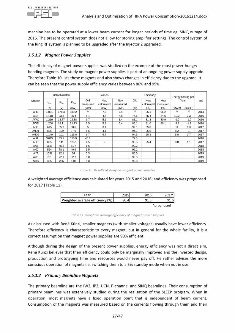
3.5.1.2 Magnet Power Supplies

The efficiency of magnet power supplies was studied on the example of the most power-hungry bending magnets. The study on magnet power supplies is part of an ongoing power supply upgrade. Therefore Table 10 lists these magnets and also shows changes in efficiency due to the upgrade. It can be seen that the power supply efficiency varies between 80% and 95%.

Table 10: Results of study on magnet power supplies

A weighted average efficiency was calculated for years 2015 and 2016; and efficiency was prognosed for 2017 (Table 11).

Table 11: Weighted average efficiency of magnet power supplies

As discussed with René Künzi, smaller magnets (with smaller voltages) usually have lower efficiency. Therefore efficiency is characteristic to every magnet, but in general for the whole facility, it is a correct assumption that magnet power supplies are 90% efficient.

Although during the design of the present power supplies, energy efficiency was not a direct aim, René Künzi believes that their efficiency could only be marginally improved and the invested design, production and prototyping time and resources would never pay off. He rather advises the more conscious operation of magnets i.e. switching them to a 5% standby mode when not in use.

3.5.1.3 Primary Beamline Magnets

The primary beamline are the IW2, IP2, UCN, P-channel and SINQ beamlines. Their consumption of primary beamlines was extensively studied during the realisation of the SLEEP program. When in operation, most magnets have a fixed operation point that is independent of beam current. Consumption of the magnets was measured based on the currents flowing through them and their

Old New New Old New Newmeasured calculated measured calculated measured

(A) (V) (kW) (kW) (kW) (kW) (%) (%) (%) (MWh) (kCHF)AHB 1‘061 178.3 189.2 1) 7.6 7.4 1) 96.1 96.2 1) 1) 2014ABS 1‘110 23.8 26.4 8.1 4.5 4.8 76.5 85.4 84.6 19.3 2.3 2016AWC 1‘219 18.77 22.88 3.7 5.1 5.4 86.1 81.8 80.9 -9.9 -1.2 2016AWD 1‘200 18.11 21.73 3.5 5.1 5.4 86.1 81.0 80.1 -9.9 -1.2 2016ANC 675 85.9 58.6 5 3.1 92.1 95.0 11 1.3 2017AND1 806 109 87.9 5.5 4.1 94.1 95.5 8.2 1 2017AND2 1‘149 101 115.8 6.7 5.7 94.5 95.3 5.8 0.7 2017AHA 3‘615 43.1 155.9 40.8 79.3 2018AHC 885 141 125.1 4.5 6 96.5 95.4 8.8 1.1 2017AXB 1143 45.2 51.7 5.6 90.2 2018AXD 524 78.1 40.9 3.5 92.1 2018AYA 1539 22.1 34 5.3 86.5 2019AYB 731 72.1 52.7 3.8 93.3 2019AIHS 385 286 110 5.8 95.0 2019

EfficiencyEnergy Saving per

YearMagnet

Betriebsdaten Losses

IBSIOut UOut POut

2015 2016 2017*90.4 91.3 91.6

*prognosedWeighted average efficiency (%)

Year


28/47

resistance (P = I2R). The current values are available in EPICS (DEVICE:IST:2 channel). The impedance values are only available in EPICS if the magnet has a digital power supply. For magnets with analogue power supply, reference resistance values were provided by M. Baumgartner. Since measurements are made at the magnets, the inefficiency of their power supplies has to be compensated for. Therefore consumption values are multiplied by 1.11. The overall consumption of primary beamline magnets is 2.3 MW. The consumption of the beamlines was measured using the SLEEP program as it was designed to monitor the power consumption of beamlines in real time. Those magnets which are not included in SLEEP were manually measured to be 217 kW, where the largest consumers are AHA (145 kW), AXB (51 kW) and AXA (12.3 kW).

Table 12: Consumption of primary beamline magnets

Figure 21: Consumption of primary beamlines in the SLEEP program

The saving potential of primary beamline magnets was studied as part of the SLEEP project. It was found that these beamlines could be optimised by further optimizing the operational usage and the handling of unexpected outages. Based on statistical and operational data of the past 3 years, it was anticipated that an average annual savings of 980 MWh could be made. Such a saving would result in the decrease of electricity cost by 118 kCHF at a price of 0.12 CHF per kWh. The SLEEP program was commissioned early 2016 and was put into production with the start of operation in May 2016.

Beamline Mangets Power (kW)Magnets outside SLEEP 217IW2 385IP2 59P-kanal 746SINQ 565UCN 125Power suppliy ineff. factor 1.1Total 2307


29/47

Figure 22: The SLEEP programs main window on 12.12.2016

As of 12.12.2016 the operation team has saved 2846 MWh using the SLEEP program. It shall be noted however, that the major SINQ outage of 2016 accounts for 1700 MWh of energy saving. This number has to be deduced from the overall savings to have a comparable value with the expected saving. 2846 MWh – 1700 MWh = 1146 MWh, which is still 15 % higher than the expected annual average.

Note that both the annual average estimation and the achieved saving are measured the magnets. In order to account for the inefficiency of magnet power supplies, they have to be multiplied by 1.11 (90% efficiency): Expected annual saving: 980 * 1.11 = 1088 MWh; actual saving: 1272 MWh.

3.5.1.4 Secondary Beamline Magnets

Beamlines MuE1, MuE4, PiE1, PiE3, PiE5, PiM1 and PiM3 are the secondary beamlines. As outlined in Section 2.3 they are supplied by transformers E2-T1, T2, T3, E1-m1 and E1-T1. The secondary beamlines serve as beamlines for experiments and their magnet configuration highly depends on the nature of the given experiments. Therefore one of the challenges was the always changing loads on most of these beamlines.

Theoretically, dedicated transformers are allocated exclusively to every secondary beamline. In reality, however, this principle was not applied and overlaps and cross-supplies occur at a number of places.

When analysing the power consumption of the secondary beamlines, the ‘top to bottom’ and the bottom up’ approaches were used in conjunction to achieve the most accurate and reliable estimation. Due to time constraints of the study, the priority of investigation was started with the largest power consumers: MuE1, MuE4 and PiE1. Typical magnet currents were obtained using the analyze program. For magnets with digital power supplies the impedance value was recorded from EPICS. In case of analogue power supplies reference resistance values were used.


30/47

MuE1 (and PiE3)

Table 13: Power consumption of MuE1 as measured at magnets

For MuE1 the typical power consumption at the magnets was found to be between 263 and 303 kW as shown in Table 13. When compared to Figure 23, the power consumption of the MuE1 transformer E1-T1, it can be seen that the beamlines consumption is approximately half of the transformer’s average power consumption. The ca 300 kW difference was investigated in depth and it was found that being labelled as MuE1, transformer E1-T1 also supplies the AHV, AHU, AHL, QHTC16, 17, 18, QHG21 and QHG22 magnets along the P-channel and SINQ (the list is not conclusive). The combined power consumption of these magnets is approximately 200 kW. It was also found that this transformer supplies power to the PiE3 beamline. Thus MuE1 ca. 300 kW + P-channel magnets ca. 200 kW + PiE3 magnets = 500+ kW, which only leaves an additional 100 kW gap between the GLS measurement point and the bottom up approximation.

Recommended measure

It is advised to further investigate the consumption of the beamline and identify all auxiliary consumers along with the power consumption of the PiE3 beamline.

Magnet BeamlineMin typical current (A)

Max typical current (A)

Resistance (Ω)

Min Typical Power (kW)

Max Typical Power (kW)

QSK82 MUE1 100 162 0.24 2.40 6.30QSK83 MUE1 -80 -130 0.02 0.13 0.34QSK84 MUE1 42 52 0.24283 0.43 0.66QSK85 MUE1 80 125 0.2433 1.56 3.80QSK86 MUE1 -176 -192 0.24 7.43 8.85QSK87 MUE1 150 210 0.24 5.40 10.58QSK88 MUE1 -35 -56 0.2409 0.30 0.76QSK81 MUE1 -48 -58 0.2425 0.56 0.82QSE81 MUE1 130 155 0.1 1.69 2.40QSK810 MUE1 -64 -95 0.24 0.98 2.17QSK811 MUE1 120 135 0.2445 3.52 4.46ASK81 MUE1 220 250 0.1441 6.97 9.01ASK82 MUE1 158 172 0.14 3.49 4.14QTH81 MUE1 275 310 0.35 26.47 33.64QTH82 MUE1 -255 -270 0.36 23.41 26.24QTH83 MUE1 140 150 0.3459 6.78 7.78ASX81 MUE1 240 265 0.25 14.40 17.56QTD81 MUE1 260 290 0.27 18.25 22.71QTD82 MUE1 -200 -215 0.26 10.40 12.02WEH82 MUE1 633 634 0.32 128.22 128.63QSK89 MUE1 -18 -20 0.24102 0.08 0.10

263 303


31/47

Figure 23: Power consumption of MuE1 in past years

MuE4 and PiE1

MuE4 and PiE1 have a common supply with an electrical multimeter at location E1.11. MuE4 branches off at E1.2 where a multimeter is also installed, but not connected to GLS. Thus any measurements on MuE4 had to be carried out manually. There were 5 manual read-off made in the time period September- October 2016, the average consumption was 120 kW. On 24.11.2016, the power consumption was measured at the magnets and at the multimeter measurement point simultaneously. It was found that measurements on magnets only showed 88 kW, while the E1.12 multimeter was supplying 153 kW of power.

Table 14: Power consumption of MuE4 as measured at magnets

Magnet BeamlineMin typical current (A)

Max typical current (A)

Resistance (Ω)

Min Typical Power (kW)

Max Typical Power (kW)

QSM610 MUE4 -84 -86 0.13 0.92 0.96QSM612 MUE4 -194 -194 0.13 4.89 4.89QSM609 MUE4 72 72 0.13 0.67 0.67QSM611 MUE4 186 186 0.13 4.50 4.50WSX62 MUE4 125 126 0.44 6.88 6.99ASR63 MUE4 268 268 0.07 5.03 5.03WSX61A MUE4 303 303 0.23 21.12 21.12WSX61B MUE4 303 303 0.23 21.12 21.12ASR61 MUE4 309 309 0.06705 6.40 6.40ASR62 MUE4 276 276 0.07226 5.50 5.50QSM601 MUE4 43 43 0.141045 0.26 0.26QSM602 MUE4 -132 -132 0.1385 2.41 2.41QSM603 MUE4 73 73 0.13856 0.74 0.74QSM604 MUE4 45 45 0.1354 0.27 0.27QSM605 MUE4 -134 -134 0.1345 2.42 2.42QSM606 MUE4 80 80 0.1337 0.86 0.86QSM607 MUE4 67 67 0.1349 0.61 0.61QSM608 MUE4 -132 -132 0.1343 2.34 2.34SEP16 MUE4 71 71 0.2312 1.17 1.17

88 88


32/47

Figure 24: Power consumption of PiE1 and MuE4 in past years

PiE1 has a more varying behaviour. Based on analyze data, consumption values range from 2 kW to 95 kW depending on the configuration of the magnets. To have comparable data from GLS, the measurement for MuE4 at E1.12 was deduced from E1.11. During the measurement of 24.11.2015, PiE1 magnets were consuming 5.8 kW, but E1.11 – E1.12 yielded 62 kW of consumption.

Recommended measures

• Connect the E1.12 meter GLS • Analyse the electrical distribution in more detail and identify the source of difference

between electrical meters and power measurements at the magnets.

PiE5, PiM1 and PiM3

Due to time constraints, the exact power consumption of these beamlines was not determined. Nonetheless, their power consumption at the relevant measurement points was evaluated on.


33/47

Figure 25: Power consumption of PiE5 in past years

Figure 25 demonstrates the strongly experiment dependant power consumption of PiE5. Previously it was observed that typically the power consumption of the magnets is 2/3 of the measured value on the electrical meter. So it is assumed that the PiE5 takes 90-100 kW.

Figure 26: Power consumption of PiM1 in past years

PiM1 can be considered as one of the most varying secondary beamline, although its overall consumption is not too significant. An average consumption of 60-70 kW is assumed.


34/47

Based on of GLS measurements since 2013, the average power for PiM3 is assumed to be 50 kW.

Recommended measure:

Analyse the electrical distribution, identify and quantify auxiliary consumers for all three beamlines.

Summary

The secondary beamlines’ power is (1) strongly dependant on the ongoing experiments and (2) time consuming to measure, due to the fact that electrical distributions can be overlapping and delivering power to other auxiliary systems. On MuE1, MuE4 and PiE1 results of the top-down and bottom-up approaches were compared. Such a comparative analysis could not be performed on other beamlines due to time constraints.

Overall, it was found that the consumption of secondary beamlines (when all in operation) is approximately 635 kW. To confirm the assumptions made in this estimation, further time investment is required. Not only would such a study confirm the assumptions, but would also identify other auxiliary systems supplied by secondary beamline transformers.

Beamline Min Typical Power (kW) Max Typical Power (kW)MuE1 260 300PiE1 and MuE4 100 190PiE5 90 100PiM1 60 70PiM3 50 50Total 560 710

Average 635


35/47

3.5.1.5 Water Cooling

A considerable power consumer is the water cooling at an average electrical power of 1.7 MWh. This electrical power is used to achieve a total cooling capacity of 12 to 15 MW. Hence the electrical power is ~ 11% of the cooling power, which at the first look can seem slightly higher than expected, but the system requires three levels of cooling to comply with regulations regarding radiation.

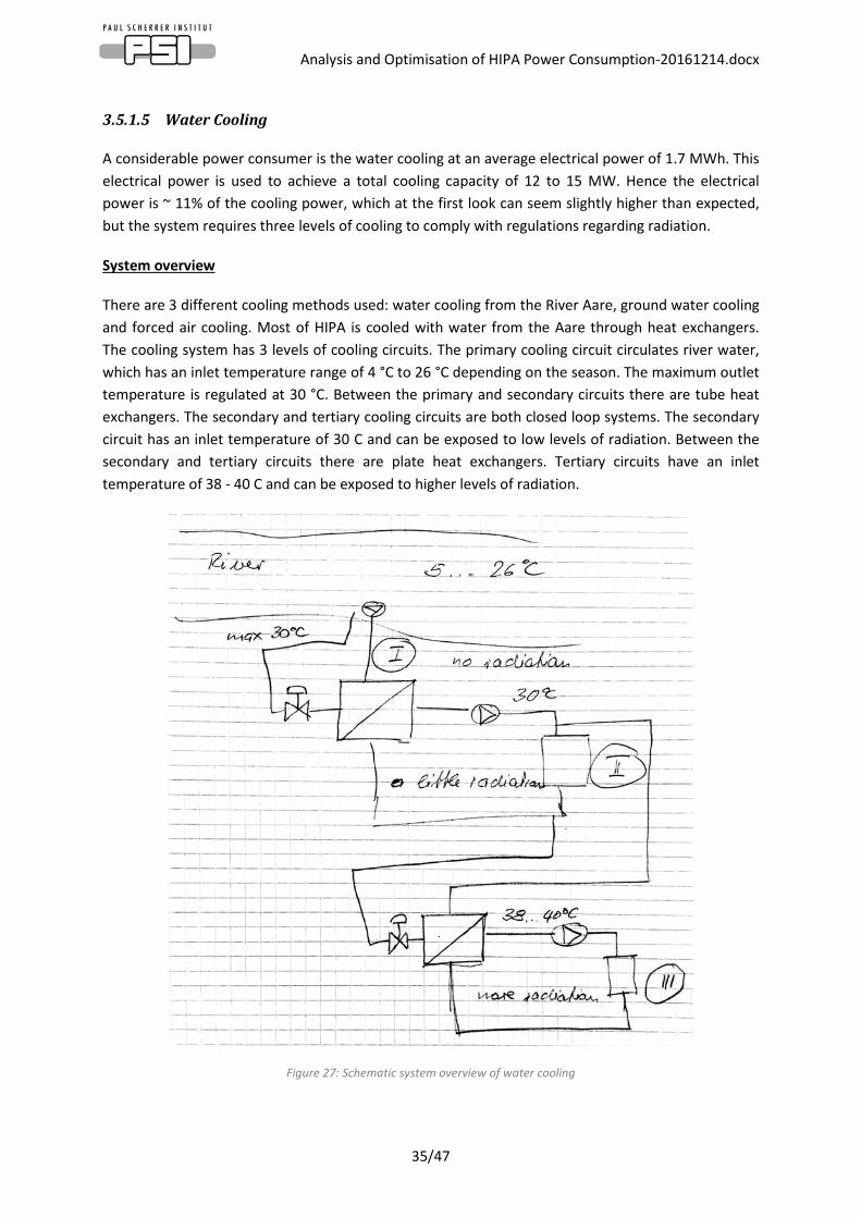
System overview

There are 3 different cooling methods used: water cooling from the River Aare, ground water cooling and forced air cooling. Most of HIPA is cooled with water from the Aare through heat exchangers. The cooling system has 3 levels of cooling circuits. The primary cooling circuit circulates river water, which has an inlet temperature range of 4 °C to 26 °C depending on the season. The maximum outlet temperature is regulated at 30 °C. Between the primary and secondary circuits there are tube heat exchangers. The secondary and tertiary cooling circuits are both closed loop systems. The secondary circuit has an inlet temperature of 30 C and can be exposed to low levels of radiation. Between the secondary and tertiary circuits there are plate heat exchangers. Tertiary circuits have an inlet temperature of 38 - 40 C and can be exposed to higher levels of radiation.

Figure 27: Schematic system overview of water cooling


36/47

Ground water (10 to 15 C depending on season) is used for air conditioners, UCN, Helium compressors and cooling of vacuum pumpstations.

Since the water cooling from the Aare only has a limited capacity, forced air cooling is also used (for injector 2 and HF). It has an increased power in summer when the Aare has a high temperature and the difference between inlet and outlet temperatures is low (small delta T) and thus cooling capacity is reduced.

Structural Analysis

Due to the large number of secondary and tertiary cooling circuits, it was possible to break down the cooling needs to sub-sections of HIPA. Although the physical layout of the cooling system is well documented, there was a lack of structural flow diagrams. Consequently s list of HIPA-relevant secondary and tertiary circuits was made and systematically drawn out to create a well perceivable structural overview as shown in Figure 27. The diagram was reviewed by A. Weber and C. Kramer.

Figure 28: HIPA Water Cooling Flow diagram

Once the list of secondary and tertiary circuits was complete, each circuit could be allocated to the area, which they supply. Percentage values of the consumption were determined based on flow rate. The detailed breakdown of the system makes it possible to evaluate the cooling of any sub-system.

Power Consumption

Flow rates, temperatures and pump currents are monitored at the pumps and the heat exchangers, therefore calculating heat and electrical power used was possible. Although managed within GLS, archived data was not available in GLS, therefore a live measurement was made at 1.2 mA beam in


37/47

October 2016 and a single measurement was made for 2.2 mA beam based on printed vale read-off from December 2015. The table below show the measurement results.

Table 15: Power consumption of cooling at 1.2 and 2.2 mA beam

Note:

• Only 2/3 of the primary Aare water circuit contributes to HIPA, hence:

𝑃𝑃 = √3 ∗ 𝑉𝑉 ∗ 𝐼𝐼 ∗ 𝑃𝑃𝑃𝑃 ∗ 23 = 200 ∗

23 = 133.4 𝑘𝑘𝑘𝑘

• Only 40% of the GW1 contributes to HIPA (same principle as above) • Forced air consumes 44 kW in summer and 25 kW in summer, hence the average 34.5 kW. • The power consumption value for SINQ was provided by F. Heinrich. The cooling of SINQ is a

stable steady load during the operation of the machine.

Cooling Circuit No.

Flow rate (l/s)

Tin (°C) Tout(°C) QheatCurrent

(A)PF

Power (kW)

Flow rate (l/s)

Tin (°C) Tout(°C) QheatCurrent

(A)PF

Power (kW)

Aarewater 155 12.8 25.7 8398 321 0.9 133.4 138 7.1 25.2 10491 321 0.9 133.4Groundwater 0 0.9 0.0 0 0.9 0.0

GW1 54.44 14 17.6 823 182 0.9 45.4 54.94 13.4 17.3 900 187.3 0.9 46.7GW2 29.4 17.6 20.5 358 73.6 0.9 45.9 28.6 17.3 21.4 492 74.7 0.9 46.6GW3 17.8 20.5 23.8 247 64.3 0.9 40.1 22.6 21.4 25.2 361 67.9 0.9 42.3GW4 0 0.9 0.0 0 0.9 0.0

Forced Air 34.5 34.5HF 0 50.8 70 0 97 0.9 60.5 50.8 70 0 97 0.9 60.5

1 14.46 29.9 40.4 638 51.3 0.9 32.0 14.82 29.9 40.4 654 51.2 0.9 31.92 Cu 16.8 30 36.3 445 91 0.9 56.7 16.03 30 36.3 424 56.1 0.9 35.0

2 28.9 28 29.9 231 52 0.9 32.4 28.84 27.9 28.8 109 91.6 0.9 57.15 21.65 28 30.2 200 87.9 0.9 54.8 21.73 28 30.2 201 81.1 0.9 50.66 0 0.9 0.0 0 0.9 0.0

6.0 54.5 29.4 34.8 1236 88.4 0.9 55.1 62.1 28.9 36.3 1930 89.5 0.9 55.86.1 54.5 29.4 34.8 1236 89.7 0.9 55.9 62.1 28.9 36.3 1930 90.3 0.9 56.36.2 54.5 29.4 34.8 1236 88.9 0.9 55.4 62.1 28.9 36.3 1930 150.2 0.9 93.76.3 54.5 29.4 34.8 1236 89.4 0.9 55.7 62.1 28.9 36.3 1930 90.1 0.9 56.26.4 54.5 29.4 34.8 1236 115.1 0.9 71.8 62.1 28.9 36.3 1930 132.9 0.9 82.96.6 39.5 30 34.7 780 240.1 0.9 149.7 39.5 29.7 37.9 1360 245.4 0.9 153.06.7 0 0.9 0.0 0 0.9 0.0

7 18.27 27.9 31.7 292 41.6 0.9 25.9 18.35 28 31.7 285 40.3 0.9 25.18 6.04 28.2 34 147 22.4 0.9 14.0 5.93 29.7 38.2 212 20.5 0.9 12.89 11.48 30 36.9 333 71.1 0.9 44.3 10.92 30 37 321 68.7 0.9 42.8

10 4.9 29.9 30.6 14 60.1 0.9 37.5 4.6 29.9 30.5 12 60.6 0.9 37.812 4 28 38.1 170 2.9 0.9 1.8 4.8 27.9 38 204 4.4 0.9 2.714 0.639 30 31.1 3 5.3 0.9 3.3 2.5 29.5 31.3 19 5.9 0.9 3.715 3 24 25.2 15 4.9 0.9 3.1 10.8 23.9 35.3 517 5 0.9 3.1

T2-Al 32.9 33.2 0 17.6 0.9 11.0 32.9 33.2 0 17.7 0.9 11.0T2 34.8 35 0 3 0.9 1.9 35 34.8 0 3.2 0.9 2.0T3 35 35 0 10.7 0.9 6.7 34.3 34.1 0 11.4 0.9 7.1T4 21.7 38 38.9 82 84.1 0.9 52.4 28.2 38 39.4 166 134.9 0.9 84.1T5 22.3 38 40.1 197 387.9 0.9 241.9 22.2 38 39.7 159 387.5 0.9 241.6T6 30 38 38 0 107.6 0.9 67.1 30 37.9 46.8 1121 112.7 0.9 70.3T7 13 38 46.8 480 30 0.9 18.7 13 37.9 48.2 562 30 0.9 18.7

SINQ Target 101.0 101.0Total 1610 1700

Normal Operation (1.2 mA beam) Normal Operation (2.2 mA beam)


38/47

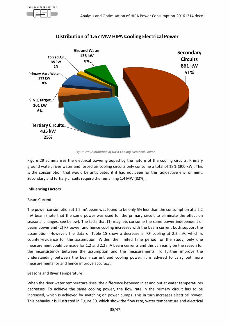
Figure 29: Distribution of HIPA Cooling Electrical Power

Figure 29 summarises the electrical power grouped by the nature of the cooling circuits. Primary ground water, river water and forced air cooling circuits only consume a total of 18% (300 kW). This is the consumption that would be anticipated if it had not been for the radioactive environment. Secondary and tertiary circuits require the remaining 1.4 MW (82%).

Influencing Factors

Beam Current

The power consumption at 1.2 mA beam was found to be only 5% less than the consumption at a 2.2 mA beam (note that the same power was used for the primary circuit to eliminate the effect on seasonal changes, see below). The facts that (1) magnets consume the same power independent of beam power and (2) RF power and hence cooling increases with the beam current both support the assumption. However, the data of Table 15 show a decrease in RF cooling at 2.2 mA, which is counter-evidence for the assumption. Within the limited time period for the study, only one measurement could be made for 1.2 and 2.2 mA beam currents and this can easily be the reason for the inconsistency between the assumption and the measurements. To further improve the understanding between the beam current and cooling power, it is advised to carry out more measurements for and hence improve accuracy.

Seasons and River Temperature

When the river water temperature rises, the difference between inlet and outlet water temperatures decreases. To achieve the same cooling power, the flow rate in the primary circuit has to be increased, which is achieved by switching on power pumps. This in turn increases electrical power. This behaviour is illustrated in Figure 30, which show the flow rate, water temperature and electrical


39/47

power of pumps as a function of time. Power consumption of the OPHB pumps peaks at 400 kW in summer and reduces to approximately 150 kW in wintertime.

Figure 30: Water Temperature, flow rate and power consumption of OPHB pumps

Secondary and tertiary circuits are not expected to change with ambient temperature, because they are ‘isolated’ circuits and their inlet and outlet temperatures can be considered constant.

Saving Potential

Power consumption of water pumps highly depend on flow rate and pressure and therefore by fine tuning these parameters cooling circuits can be optimised. Such an optimisation requires the pumps to be frequency driven to be able to set operation point along the pressure – flow rate curves. At the moment only secondary circuits no. 14 and 15 and the air cooling units have variable frequency drive. The rest of the pumps were installed around 2000 and have a lifespan of approximately 20 years. Therefore their replacement is planned to start in 2020, where the new pumps will have frequency driven control. Modifications to the cooling loops will also be required to be able to apply feedback based on pressure drop across the load. A. Weber expects that when all pumps are upgraded to VFD, the electrical power consumption should decrease by roughly 20%. Excluding SINQ pumps and those which already have VFD, the expected reduction is 300 kW. Over a period of one year, this could result in 0.3 MW * 24 h * 30 * 8 = 1.7 GHh of saving on electricity on HIPA and additional saving on other systems supplied by the same primary circuits. Note this is a rough estimation; to find the saving potential more precisely, it is advised to conduct a separate study on the optimisation of the cooling system. Although the upgrade is only planned to start in 2020 and be conducted over a number of years, the large saving potential might justify an earlier updated and might provide access to more resources.


40/47

3.5.1.6 Cryogenics

There are three cryogenics systems related to HIPA. KA1 is responsible for SINQ, KA2 for UCN and KA4 for the experiment area MuE1 and liquefying helium for other experimental areas.

In cryogenic cooling the biggest portion on power is taken up by the compressors, which put in the work at the beginning of the cooling process to compress Helium. Table 16 below shows how power is distributed between the compressors and the auxiliary systems (pumps, motors, cooling, etc).

Table 16: Power consumption of cryogenic systems. Data courtesy of C. Geiselhart, apart from *, which was manually measured on the S5.21 distribution

Cryogenic systems run 24/7/365 when HIPA is in operation, because switching off and on is a time consuming operation, furthermore, when switched off much maintenance and cleaning has to be done before it could be switch on again. Therefore it is not worth switching cryogenics off for less than a month; not to mention the mechanical stress on the materials when cycled between sub-20K and room temperature on a regular basis. Usually cryo-cooling is switched on 3 weeks before the end of HIPA shutdown, since it is a time consuming procedure and there is some slack left for unforeseen issues.

The compressors used at the moment are 40 years old and hence they are approaching the end of their lifespan and technology has advanced considerably in the last decades. Therefore an upgrade of KA1 and KA4 is planned for the long shutdown of 2018. With an upgrade to screw compressors, it is expected to increase in efficiency by 20% as well as the new machines will not be water, but air cooled, which also result in a decreased consumption and less maintenance will work. Overall it is estimated by C. Geiselhart that 180 kCHF will be save on an annual basis. This savings number comprises of the power saved, the saving on chemicals (cleaning cooling water) and reduced amount of maintenance work. CAPEX is expected to be 2.1 million CHF (compressors 1.6-1.7 million CHF). When implemented, a return of 600 kCHF will be gained from the ProKilowatt Program (http://www.bfe.admin.ch/prokilowatt/04344/index.html?lang=de).

As far as energy is concerned, the 20% reduction translates to (240 + 540) * 0.2 = 156 kW. Hence the annual saving is 0.156 * 24 * 30 * 8 = 900 MWh assuming 8 months of continuous operation.

If successful, C. Geiselhart believes a similar upgrade would be possible for the UCN compressors as well, however, those compressors would not fit into the WKSA building, and therefore its implementation will be more complicated and might require larger investment (new building).

Nr. Name TypeRated Motor Power (kW)

Motor Power during Normal Operation (kW)

Auxiliary Systems (kW)

Total power (kW)

KA1 SINQ Labyrinth 360 240 30 270KA2 UCN Labyrinth 450+50 370 - 370KA4 Mue1 (+experimLabyrinth 630 540 30 570Total Power (kW) 1210

http://www.bfe.admin.ch/prokilowatt/04344/index.html?lang=de


41/47

3.5.1.7 Vacuum

The vacuum system consists of a large number of vacuum pumps and pre pumps as well as cryogenic pumps. The power of the pumps can vary depending on the mode of operation. In standard operation, pumps require a moderate but continuous power. When ‘pumping up’, power increases considerably for a relatively short period of time. Consumption values were estimated by P. Rüttimann by taking into account both modes of operation and are shown in Table 17.

Table 17: Vacuum system inventory with power consumption. Accuracy: 10%, data courtesy of P. Rüttimann

Given the relatively modest power consumption and the time constraint of the present study, the saving potential of the vacuum system was not addressed.

3.5.1.8 Pressurised Air

The pressurised air system has three compressors for producing high pressure air. At a time two of the compressors are in operation, the third one is for redundancy reasons. Out of the total 440 m3/h production average, 293 m3/h is assumed to be relevant to HIPA. At a specific power of 0.13kW/m3/h, the yearly estimated consumption is 293 m3/h * 8760 h * 0.13 kW/m3/h = 334 MWh for the pumps. The dryer consumes 0.4 kW and thus contributes an additional 2/3 * 0.4 * 8760 = 2.4 MWh, yielding a total of 336 MWh over a year. The estimated instantaneous power is 38.4 kW. Given the relatively modest power consumption and the time constraint of the present study, the saving potential of the pressurised air system was not addressed.

3.5.1.9 Ventilation

Ventilation is an essential part of the HIPA infrastructure. Experiment halls, SINQ, accelerator bunkers and beamline tunnels have to be ventilated, not only for a reason of convenience, but also for safety reasons. Large primary ventilation units are installed on the outside of buildings. These units filter and heat air if necessary. Unlike SLS, HIPA does not have specific hall temperature requirements as the facility is not temperature dependant. Heating is mostly applied during shutdown, when the facility does not dissipated heat that would warm up the experiment halls. During normal operation the heat dissipation of the machine is enough to keep the hall warm. It

Consumer Number Power per device (kW) Power (kW)Turbo Pumpen TCP350 Durchschnitt 60 0.4 24Turbo Pumpen 2000 1 1 1Kryopumpen 10000 4 8 32Kryopumpen 2000 6 4.5 27Vorpumpen 15 45 0.02 0.9Vorpumpen30 1 0.03 0.03Vorpumpen Schrauben 300 2 0.275 0.55Vorpumpen Roots 2000 1 0.1375 0.1375Vorpumpen Schrauben 100 2 0.123 0.25Vorpumpen Roots 500 1 0.06 0.06Measurement devices 70 0.0015 4.2Total Power 90


42/47

results in a varying hall temperature throughout the year. Since there is on central air conditioning installed, in summer the hall temperature follows the ambient temperature.

The power consumption of the ventilation system was preliminarily studied and it was found to consume approximately 190 kW (estimated by group of D. Reinhard). This was obtained on a single measurement in October 2016. The accuracy of the measurement could be further improved and verified, but it was prevented by personnel illness. Nonetheless the areas where savings could potentially be made were discussed in greater detail with D Reinhard:

• Reducing the flow rate of ventilators could reduce electrical power, however, ventilation play a safety role therefore such actions are not allowed.

• In principle ventilation could be reduced in neutron halls, where it is not safety critical. • Optimisation of filters: The filter with a lower pressure drop can reduce electrical power

needs. The pre-filters of the large ventilation units are already life cycle optimised. The main filters are also believed to be one of the best choices available on the market, however, with little effort it could be confirmed. In case there are better options, the saving potential is still small. Note that during filter optimisation the lifespan of filters also has to be taken into account given the labour intensive (and hence costly) maintenance work.

• Optimising control: Some ventilation units do not have frequency control, but only throttle control, in such cases, potential could be medium (large compared to the units present consumption). Has to be individually checked for every ventilation unit. Note the main ventilation units already have frequency control.

3.5.1.10 Air Conditioning

Although there is no central air conditioning in place, certain areas of HIPA require conditioned air. AC units are installed locally where air cooling is needed. These units can be water cooled AC units, monoblocks, split or window AC systems. They are partially managed by the building technology section (Gebäudetechnik) and by Hall Services (Hallendienst).

The consumption of the prior AC units was estimated to be 167 MWh per annum (see composition in Appendix ?). These units are mostly used irregularly throughout the year. Their large number and relatively low consumption makes further analysis unnecessary. The annual average consumption is assumed to be 167 MWh / 8760 h = 19 kW, with a maximum peak power of 81 kW.

Smaller window AC systems (maintained by Hallendient) are used for cooling experiment hutches, server and control racks etc. The list of smaller split AC systems can be found in Appendix ? (list provided by B, Jehle. There are 35 such AC units in the HIPA area. All of them are the same model from the same supplier (ZHENDRE W18AV), but their age varies from 2 to 15 years. Based on the manufacturer’s data plate, the cooling power is 5275 W or 18000 BTU/h. The maximum electrical power is 2.45 kW, but normal operation only requires 2.3 kW. 80% percent of these devices run only during machine operation and 20% runs all around the year. The power during normal operation is 35 * 2.3 = 82 kW, power during shutdown is 0.2 * 82 = 16.4 kW. Therefore the calculated energy consumption is (82 * 24 * 30 * 8 + 16.4 * 24 * 30 * 4) / 1000= 472MWh + 47.2 MWh = 520 MWh.

After a small market research, it was found that there are much more efficient AC units available, with the same 18000 BTU rating, but around 1.6kW consumption (example: LG LW1815ER). Compared to the 2.3kW consumption of the ZHENDRE units, a potential for energy saving is clear:


43/47

• During normal operation: 35 units x 0.7 kWh difference per h x 24 hours a day x 30 days a month x 8 months of operation = ca 141,000 kWh = 141 MWh.

• During shutdown: 7 units x 0.7 kWh difference per h x 24 hours a day x 30 days a month x 4 months of shutdown= ca 14,100 kWh = 14 MWh.

• Total saving potential of 155 MWh/year

The LG unit has a $500 retail price in the US. Assuming 800 CHF price per unit the CAPEX cost is ca 28,000 CHF for the AC units + another 28,000 CHF manpower = 56,000 CHF. Given an energy price of 0.12 CHF/kWh, the annual return is ca 18,600CHF/year. Therefore the ROI is 56,000/18,600 is 3 years.

The preliminary market research is a good indication of the saving potential, but it is recommended to conduct an extensive market research, CAPEX and OPEX analysis considering factors such as reliability, filter lifetime and maintenance.

Add photo

3.5.1.11 Lighting

The lighting in the HIPA facility has undergone a number of upgrades in recent years and hence it is already highly optimised as outlined by E. Hüsler. The experiment hall lighting was upgraded in 2011/12. The new system features dimmable fluorescent tubes, whose brightness is adjusted based on the amount of ambient light coming through the windows. Lighting in the experiment halls consumes 340 MWh annually, which equates to 340 MWh / 8760 h = 38 kW. It should be noted that power is necessarily higher in the night and lower during the day. Figure 31 shows the fluctuations in power for the E1.6 Infrastructure distribution cabinet. The power required for lighting is also expected to vary with the season. This assumption could only be proven if lighting was metered separately.

Figure 31: Daily power fluctuation of E1.60, source: GLS egli tool.

At the time of the experiment hall modernisation, upgrading to LED technology was not viable due to high CAPEX. By 2014, technology and LED mass production has largely advanced and the lighting in neutron halls WNHA and WLNA was upgraded to LED lights. The annual electricity used is 96 MWh, yielding an average of 96 MWh / 8760 h = 11 kW.

Thus the total power consumption of lighting is 436 MWh; or 436 MWh / 8760 h = 50 kW.


44/47

The possible upgrade of neutron hall lighting could be studied and CAPEX and OPEX could be compared. It is expected that OPEX of LED light is considerably lower since LED bulbs have considerably higher lifetime than fluorescent tubes.

3.5.1.12 Other Infrastructure and Instrumentation

As outlined is Section 245 kW of infrastructure is assumed to be consumed by heating, control systems, wall plugs at experiment areas and other infrastructure. Although this un-measured and/or un-known infrastructure only accounts for 2% of the facility’s consumption, it could be further reduced if electrical distributions cabinets are studied in greater detail.

3.6 Comparison of Approaches and Energy Consumption The analysis process facilitated both a bottom-up and a top down approach. The bottom-up approach first looked at the list of consumers and then measured, calculated or estimated their power consumption, irrespective of their position in the electrical distribution ‘pyramid’. The top-down approach started with the analysis of the supply grid and attempted to allocate every transformer (or power distribution) to a specific sub-system of HIPA. Whether or not the allocation could be made, the combined consumption of the facility could be obtained by adding up the HIPA relevant power consumers.

For every meter available in GLS, the energy counter value was obtained through the egli too for the past three years. Energy counter values were recorded for 1 January and 1 May for every year. This allowed for calculating the average power during shutdown and maintenance periods. Results are summarised in Table 18.

Table 18: Measured consumption of HIPA in 2013, 2014 and 2015

Location Rack No. Source (if any) Name Label UseService

(kW)Operation

(kW)Consumption

(GWh)Service

(kW)Operation

(kW)Consumption

(GWh)Service

(kW)Operation

(kW)Consumption

(GWh)

WSGA S5.1 S5.2 Kühlcentrale Hausbedarf CoolingWSGA S5.2 Trafo S1-T15 Trafo S1-T15 Hausbedarf Cooling + Building Infrast. 348 944 6.44 303 922 6.19 394 928 6.48WSGA S5.12 ? ND Verteiler HV UCN Exp Hausbedarf

WSGA S6.17 Trafo S1-T14 Trafo S1-T14 Ring + Injector Magnets 127 955 5.87 95 939 5.68 170 909 5.72WSGA S6.18 S6.17 Hauptspule Ring + Injector Main Coils

WSGA S5.19 Trafo S1-T11 Trafo S1-T11 Bio Medizin UCN 142 560 3.63 73 380 2.40 41 486 2.92WSGA S5.20 S5.19 HV UCN Exp. Feld WMFA:H:20 Bio Medizin UCNWSGA S5.21 S5.19 HE Komp Anlage 2 Feld WMFA.H.10 Bio Medizin UCN HE Kompressor KA2

WSGA S6.1 Trafo S1-T12 Trafo S1-T12 P-Kanal + Exctract. P-Kanal + Exctraction 0 720 4.15 0 720 4.15 0 720 4.15

WSGA RF S82.13 Trafo S1-T13 Trafo S1-T13 ring HF pre-amps RF Included in Ring RF below Included in Ring RF below Included in Ring RF below

WNHA Gallery 2 West NH2.13.21 NH2.13 Z3 NS-Verteilung Hausbedarf SINQ Infrastructure 147 233 1.77 136 230 1.72 138 229 1.71WNHA Gallery 2 West NH2.12.21 NH2.13 Z1 NS-Verteilung Hausbedarf SINQ magnets 34 448 2.68 18 482 2.83 20 485 2.85

WEHA Gallery 2 East E1.50 Trafo WEHA E1-T2 MuE1 MuE1 26 559 3.30 25 638 3.74 44 582 3.48WEHA Gallery 2 East E1.6 Trafo WEHA E1-T1 Exp/Infrastructure Infrastructure Infrastructure 242 569 3.98 230 584 4.03 301 570 4.15WEHA Gallery 2 East E1.5 NotstromWEHA Gallery 2 East E1.11 Trafo E1 M1 PiE1 Axe 5-6 PiE1 Axe 5-6 PiE1 7 156 0.92 16 180 1.09 23 165 1.02WEHA Gallery 2 East E1.12 E1.11 NS Verteiler MuE4 E4.1 MuE4

WEHA Gallery 2 West E2.1 Trafo E2-T1 PiM1 Axe 6/6 PiM1 Axe 6/7 PiM1 1 48 0.28 2 54 0.32 3 46 0.27WEHA Gallery 2 West E2.31 Trafo E2-T3 PiM3 Axe H 8-8 PiM3 Axe H 8-9 PiM3 5 52 0.31 3 51 0.30 6 48 0.30WEHA Gallery 2 West E2.41 Trafe E2-T2 HV PiE5 Axe H9-10 HV PiE5 Axe H9-11 PiE5 27 194 1.19 36 154 0.99 11 113 0.68

WIHA G60.20 Trafto G1-T1 Trafto G1-T1 Inj2 Maschine + Allgemeine 98 499 3.15 117 466 3.02 148 474 3.16WIHA G60.01 Trafto G1-T1 Trafto G1-T1 Inj2 Maschine + Allgemeine 29 196 1.22 32 194 1.21 78 188 1.31WIHA G60.29 G60.20 Hausbedarf Infrastructure 7 42 0.26 37 41 0.34 32 38 0.31WIHA G60.12 G60.01 Notenetz Energency equipment

WIHA CW C3.2 Cockroft Walton Cockroft Walton 0 15.6 0.09 0 15.6 0.09 0 15.6 0.09Inj2 15 kV amp 72 561 3.44 78 548 3.38 109 577 3.64Ring RF 0 3850 22.18 0 3850 22.18 0 3850 22.18Cryo KA1 (SINQ) 0 270 1.56 0 270 1.56 0 270 1.56Cryo KA4 (MuE1+Exp.) 0 570 3.28 0 570 3.28 0 570 3.28Pumping House 62 153 1.06 63 157 1.08 68 159 1.11

TOTAL 1368 11552 70 1228 11405 69 1554 11384 70

2013 2014 2015


45/47

Average power was calculated by taking the difference between two consecutive measurements and dividing it by the time period between the measurements. Note that in a number of cases measurements were not available and the following assumptions were used:

• Transformer S1-T12: Due to the fault in the measurement device the only and most recent measurement is for 2014. The same consumption was hence used for 2013 and 2015

• Ring RF is not measured on the 16 kV side, so finding its power in GLS was not possible. The archived RF forward power was analysed by averaging measurements over the machine operation period in 2015. The average forward RF power was 1925 KW, hence the grid power was estimated to be 3850 kW.

• For the cryo cooling machines KA1 and KA4 power was assumed to be 270 kW and 570 kW during normal operation, respectively. For shutdown zero consumption was assumed.

The average power during operation was ca 11.5 MW in the past three year. This is 1 MW higher than the 12.5 MW obtained through the bottom up approach. The difference can be explained by the fact that the 12.5 MW is an instantaneous value when every sub-system is running, while the 11.5 MW includes outages and planned services too.

The annual consumption of HIPA was roughly 70 GWh in the past years based on GLS measurements. This is a useful value because it mostly adds up from individual measurements; however, a major part (RF 20+ GWh) is not as accurate as the rest, because of the RF efficiency assumption using the value of 2015 instead of averaging the three years. Finding average RF forward power for every year can further improve accuracy.


46/47

3.7 Summary of Saving Measures and Further Work A number of areas have been identified, where saving could be made and also others where further investigation can help to optimise and better monitor the facility. At the same time it is important to admit that the operation of the HIPA facility has been already highly optimized in the last several years. Note: suggested further works are marked with indented fonts.

Figure 32: Distribution of 4 GWh HIPA Saving Potential

Figure 32 shows the distribution of the 4 GWh saving potential of the facility. The largest saving potential lies in optimising the cooling system with introducing VFD (variable frequency drive) pumps. This requires a high investment, but the annual 1.7 GWh saving also translates to a high (ca. 200 kCHF per year) return. To assess its saving potential more precisely, it is recommended to conduct a separate study. The second potential is energy optimisation of the primary beamline magnets, which has been already implemented in the SLEEP project and resulted in saving 1272 MWh of electricity in 2016. SLEEP has been upgraded with a newly implemented RF module. It will assist operators to make as much as 370 MWh of additional saving besides documenting the amounts, which have already been saved. The upgrade of cryogenic compressors KA1 and KA4 to screw compressors will increase efficiency by 20% from 2018 onwards. A relatively small, but certain saving can be made by upgrading the 35 window AC systems in the experiment hall to modern equivalents. A precise estimation of the saving potential and the payback period can be analysed in a standalone study.

Other measures can contribute to the optimisation of the facility, although their impact cannot be quantitatively expressed:

• Introducing new electrical measurement points to the electrical grid can greatly increase our understanding of the machine’s energy flow. A better understanding also means more precise monitoring and thus the 1) easier detection of measurement faults, 2) better and more accurate reporting on the energy consumption and performance of large research facilities and 3) more powerful analysis tools to identify areas of further saving. Suggested places for additional meters are detailed in Section 2.3.

• Further studying and analysing the consumers of secondary beamline (and other) transformers, where the power consumption cannot be fully accounted for as of new.


47/47

• The ‘accelerated’ implementation of the e3m energy measurement concept can provide the tools to visualise the abovementioned improved monitoring and reporting system

• The upgrade of Ring RF amplifier control system would make the optimisation on amplifier feasible. A single optimisation to a new operating point can decrease grid power by 200 kW.

• Including the cooling circuits of the Injector 2 upgrade can increase the harvested heat through heat recovery (further study recommended)

4 Conclusion

The study has addressed all of its aim and has elaborated on them to a great extent. The analysis of the electrical grid was done using a top to bottom approach. The analysis first revealed the clear structure of the 16 kV PSI supply line with the HIPA-specific supply ring. HIPA-relevant transformers were identified and compiled in an inventory list. The electrical distribution of every element of the list was identified along with the major consumers. If an electrical meter was installed, it was also identified in the GLS system. Depending on the specific configuration and consumers of the distribution cabinet, the introduction of further electrical multimeters was suggested.

In order to find the total power of the facility, a comprehensive list of sub-consumers was created. First these consumers were classified into the following categories: accelerator, auxiliary and Infrastructure. The power consumption of every sub-system was identified and areas of saving were also determined. The dependency of the sub-systems’ power on factors such as beam power and season was also addressed. By summing up the power of all sub-systems, the 12.5 MW power consumption of HIPA was found.

Of similarly high interest was to determine the accelerators efficiency at the production of a minimum full beam. In this calculation only those parts of the facility were taken into account, which are minimally essential to produce a 2.2 mA beam at the extraction from the Ring. The grid to beam efficiency of such a setup is 18.3% at a total power of 7.1 MW. This has a high scientific significance, because it can be used as a reference value for efficiency of high intensity accelerators in general.

energy efficiency analysis and optimisation of hipa power

Documents