deposit_hagenPublikationsserver der Universitätsbibliothek

Mathematik und Informatik

Dissertation

Patrick Eitschberger

Energy-efficient and Fault-tolerant Scheduling for Manycores and Grids

FernUniversität in HagenFakultät für Mathematik und Informatik

Lehrgebiet Parallelität und VLSI

Energy-efficient and Fault-tolerantScheduling for Manycores and Grids

Dissertationzur Erlangung des akademischen Grades

DOKTOR DER NATURWISSENSCHAFTEN(Dr. rer. nat.)

vonDipl. Inform. Patrick Eitschberger, M. Comp. Sc.

Dorsten

Hagen, 2017

Promotionskommission:Erster Gutachter: Herr Prof. Dr. Jörg Keller

(FernUniversität in Hagen, Germany)Zweiter Gutachter: Herr Prof. Dr. Christoph Kessler

(Linköping University, Sweden)Vorsitzender der Promotionskommission: Herr Prof. Dr. Friedrich SteimannPromovierte Mitarbeiterin: Frau Dr. Daniela Keller

Tag der Disputation:05. Oktober 2017

II

For my wife Katrin andmy children Milian and Jannis

III

Abstract

Parallel platforms like manycores and grids consist of a large number of processingunits (PUs) to achieve high computing power. To enable a fast execution of complexapplications, they must be decomposed into several tasks and scheduled efficientlyonto the parallel platform.

The reliability of these platforms is crucial in order to avoid high costs in senseof money, time or life-critical situations. A failure of a PU can be tolerated by taskduplication, where each task is duplicated onto another PU. In case of a failure,the schedule execution can be continued by running the duplicates instead of thefaulty original tasks. But integrating duplicates into a schedule often results inperformance overhead already in the fault-free case.

Additionally, a low energy consumption for a schedule is desired to reduce costsand to protect the environment. Dynamic voltage and frequency scaling (DVFS)is one approach to reduce the energy consumption. However, scaling the frequen-cies and voltages of PUs to an efficient level often leads to performance overhead,because tasks are usually slowed down. In addition, including duplicates into aschedule increases the energy consumption because they are typically executed be-side the original tasks. This leads to a three-dimensional optimization problem ofperformance, fault tolerance and energy consumption.

In this thesis the interplay between these three objectives is explored. Severalnew fault-tolerant and energy-efficient heuristics and strategies are presented thatoffer a user the opportunity to set various preferences. Additionally, a prototyperuntime system is presented that tolerates a failure and also uses DVFS to improvethe energy consumption. Finally, the different strategies are evaluated with varioustest sets in general but also with real-world applications on real parallel platforms.

IV

Zusammenfassung

Parallele Systeme, wie beispielsweise Manycores und Grids, bestehen aus einergroßen Anzahl an Verarbeitungseinheiten (PUs), um eine hohe Rechenleistung zuerzielen. Um eine schnelle Abarbeitung komplexer Applikationen zu ermöglichen,müssen diese in mehrere Tasks zerlegt und effizient auf die parallele Plattform einge-plant werden.

Die Zuverlässigkeit dieser Plattformen ist entscheidend, um hohe Kosten im Sinnevon Geld, Zeit oder lebensbedrohlichen Situationen zu vermeiden. Ein Ausfall einerPU kann durch Task-Duplikation toleriert werden, bei der jede Task auf einer an-deren PU dupliziert wird. Im Falle eines Ausfalls kann die Schedule-Verarbeitungfortgesetzt werden, indem die Duplikate anstelle der ausgefallenen Original-Tasksausgeführt werden. Allerdings führt das Einfügen von Duplikaten in einen Schedulebereits im fehlerfreien Fall häufig zu einem Leistungsverlust.

Zusätzlich wird ein niedriger Energieverbrauch für einen Schedule angestrebt, umKosten zu reduzieren und die Umwelt zu schonen. Dynamische Spannungs- undFrequenzskalierung (DVFS) ist eine Möglichkeit, um den Energieverbrauch zu re-duzieren. Jedoch führt die Skalierung der Frequenzen und Spannungen von PUshäufig zu einem Leistungsverlust, da Tasks für gewöhnlich verlangsamt werden.Außerdem erhöht das Einfügen von Duplikaten in den Schedule den Energiever-brauch, da sie in der Regel neben den Original-Tasks ausgeführt werden. Dies führtzu einem drei-dimmensionalen Optimierungsproblem zwischen Leistung, Fehlertol-eranz und Energieverbrauch.

In dieser Arbeit wird das Zusammenspiel zwischen diesen drei Zielen erforscht.Mehrere neue fehlertolerante und energieeffiziente Heuristiken und Strategien wer-den präsentiert, die einem Benutzer die Möglichkeit bieten unterschiedliche Präferen-zen einzustellen. Darüber hinaus wird ein prototypisches Laufzeitsystem vorgestellt,das einen Fehler toleriert und DVFS benutzt, um den Energieverbrauch zu verbessern.Zum Abschluss werden die unterschiedlichen Strategien mit verschiedenen Testmen-gen im Allgemeinen aber auch mit realen Anwendungen auf realen parallelen Platt-formen evaluiert.

V

Acknowledgement

I would like to thank in particular Prof. Dr. Jörg Keller for his great supervision andthe countless fruitful discussions, helpful hints and his untiring patience (especiallyin the final phase of my Ph.D.) during my time as a research assistant and Ph.D.-student in his research group.

Many thanks to Prof. Dr. Christoph Kessler for interesting discussions, ideas andinsights in related topics, which have positively influenced the development of thisthesis. Thanks for agreeing to be the second reviewer of this thesis.

I am grateful for the detailed discussions with Dr. Simon Holmbacka related toseveral parts of this thesis, like power modeling of real systems, trade-off analysisand estimation of lower/upper bounds. This helped me to find new ideas and toimprove the quality of this thesis. Thanks for also proof-reading most of the partsof this thesis.

I like to thank Prof. Dr. Wolfram Schiffmann and Dr. Jörg Lenhardt for the dis-cussions and feedbacks about energy modeling. Special thanks to Dr. Jörg Lenhardtfor his feedback to several questions related to LATEX and for proof-reading this the-sis.

I especially would like to thank my lovely family for the support and motivationduring my Ph.D.-study. Special thanks to my wife Katrin, who gave me the neces-sary freedom to write down this thesis and who always listened to me, when I hadproblems. Warm thanks to my children Milian and Jannis, who brought a smile tomy face whenever I was stressed or unmotivated.

Thanks to all not explicitly mentioned persons, who supported me during thistime.

Patrick EitschbergerHagen

June 5, 2017

VI

Publications and Previous WorkParts of the work described in this thesis have been published in the followingarticles. After a short description of the content, the contribution of the authorsis described for each publication. All parts in this thesis that are related to thesearticles are explicitly cited. The sections that cover the work in the articles are givenfor each article.

Patrick Cichowski, Jörg Keller, Christoph Kessler: Modelling Power Consumptionof the Intel SCC. 6th Many-core Applications Research Community Symposium(MARC ’12), Toulouse, France, Jul. 2012, pp. 46-51 [45] (covered in Sect. 6.3.2).

In this article, a power model for the Intel SCC (Single-chip Cloud Computer)is presented. Based on the results of several micro-benchmarks and workloaddistributions over all cores the tuning parameters for the proposed power modelare determined by a least squares analysis.

This publication was written by Patrick Cichowski, Jörg Keller and ChristophKessler. Jörg Keller suggested the power model and the micro-benchmarks forthe Intel SCC. Christoph Kessler contributed several details about the IntelSCC and related work. Patrick Eitschberger implemented and evaluated themicro-benchmarks and gave further information of the SCC.

Patrick Eitschberger, Jörg Keller: Efficient and Fault-tolerant Static Scheduling forGrids. 14th IEEE International Workshop on Parallel and Distributed Scientificand Engineering Computing (PDSEC ’13), Boston, Massachusetts, May 2013, pp.1439-1448 [53] (covered in Sects. 2.4.3, 4.2.1 and 4.2.3).

In this article, a fault-tolerant duplication-based scheduler is presented thatguarantees no overhead in a fault-free case. Based on the approach of Fechneret al. [59] where no communication time is considered, the influence of the com-munication time between tasks onto the placement of duplicates is discussedand different strategies are presented. Additionally, in this paper another kindof fault is introduced where tasks can be slowed down because of a high usagerate of a processor. In this case, the already placed duplicates can be used tospeedup the execution.

This publication was written by Patrick Eitschberger as most of the resultswere based on his German diploma thesis. Jörg Keller proof-read the paperand checked the writing style. He furthermore contributed the idea of usingthe duplicates for slowed down tasks. Patrick Eitschberger implemented andevaluated this extension.

VII

Patrick Eitschberger, Jörg Keller: Energy-efficient and Fault-tolerant Task GraphScheduling for Manycores and Grids. 1st Workshop on Runtime and OperatingSystems for the Many-core Era (ROME ’13), Aachen, Germany, Aug 2013, pp.769-778 [54] (covered in Sects. 4.3.1 and 4.3.4).

In this article, as an extension, frequency scaling is included into the previousapproach [53] to either improve energy consumption in the fault-free and faultcase or the performance overhead in case of a failure. The frequency for tasks isscaled down without prolonging the makespan of the original schedule. In caseof a failure tasks can also be speeded up to reduce the performance overhead.

This publication was written by Patrick Eitschberger. He also contributedthe main idea of integrating energy efficiency aspects, i.e. frequency scalinginto the fault-tolerant scheduler and the corresponding heuristic. Jörg Kellercontributed details for a generalized power model and suggested to also usefrequency scaling for speeding up tasks in case of a failure. The implementationand evaluation was done by Patrick Eitschberger.

Christoph Kessler, Nicolas Melot, Patrick Eitschberger, Jörg Keller: Crown Schedul-ing: Energy-Efficient Resource Allocation, Mapping and Discrete Frequency Scalingfor Collections of Mallable Streaming Tasks. 23rd International Workshop on Powerand Timing Modeling, Optimization and Simulation (PATMOS ’13), Sept 2013, pp.215-222 [104] (used as related work in Sect. 2.5.3).

In this article, an energy-efficient optimization approach, called crown schedul-ing, for malleable streaming tasks is presented. Crown scheduling is based oninteger linear programming (ILP) and combines next to a separate consider-ation the resource allocation, mapping and discrete voltage/frequency scalingunder a given throughput constraint.

This publication was written by Christoph Kessler and Jörg Keller. ChristophKessler contributed an ILP model for the separate and combined crown schedul-ing. Patrick Eitschberger developed a task set generator for the experimentalsection and participated in combining the software for the separate phases.Nicolas Melot implemented and combined the separate phases of crown schedul-ing. He also adapted details of the ILPs and evaluated crown scheduling.

Nicolas Melot, Christoph Kessler, Jörg Keller, Patrick Eitschberger: Fast CrownScheduling Heuristics for Energy-Efficient Mapping and Scaling of Moldable Stream-ing Tasks on Manycore Systems. ACM Transactions on Architecture and Code Op-timization (TACO ’15), vol. 11, no 4, pp. 62:1-62:24, Jan. 2015 [126] (used asrelated work in Sect. 2.5.3).

VIII

In this article, the previous approach [104] is extended by several phase-separatedand integrated heuristics for Crown Scheduling. The longest Task, lowest Group(LTLG) heuristic is introduced to balance the load for mapping parallel tasks.A Height heuristic is presented for frequency scaling. The allocation is opti-mized by heuristics based on binary search and simulated annealing.

This publication was written by Nicolas Melot. He designed the optimal alloca-tion and the phase-separated and integrated heuristics for Crown Scheduling.Christoph Kessler contributed the concrete task set in the extended experimen-tal section. Christoph Kessler, Patrick Eitschberger and Jörg Keller proof-readthe paper and checked the writing style.

Patrick Eitschberger, Jörg Keller: Energy-efficient Task Scheduling in ManycoreProcessors with Frequency Scaling Overhead. 23rd Euromicro International Con-ference on Parallel, Distributed, and Network-Based Processing (PDP ’15), Turku,Finland, March 2015, pp. 541-548 [55] (covered in Sect. 2.5).

This article focuses on evaluating the overhead in time and energy that is spentfor frequency scaling. Especially for small time scales the frequency scalingoverhead can have a significant influence on the runtime and energy of a sched-ule. With the help of a bin packing heuristic the frequency scaling overhead isconsidered and optimized schedules are created.

This publication was written by Patrick Eitschberger and Jörg Keller. JörgKeller contributed the idea to use bin packing and participated in interpretingthe results. Patrick Eitschberger contributed to the cost function for the binpacking. He also implemented and evaluated the bin packing heuristic.

Patrick Eitschberger, Jörg Keller: Fault-tolerant Parallel Execution of Workflowswith Deadlines. 25th Euromicro International Conference on Parallel, Distributed,and Network-Based Processing (PDP ’17), St. Petersburg, Russia, March 2017, pp.541-548 [56] (covered in Sects. 4.3.6, 4.3.7, 4.3.8 and 4.5).

In this article, the previous work in [53] and [54] is extended by several ap-proaches to improve the energy consumption in case of a failure. Next tovarious heuristics also ILPs for optimal solutions are presented.

This publication was written by Patrick Eitschberger and Jörg Keller. JörgKeller contributed the idea and implementation of the CP-heuristic (Con-stant Power). Patrick Eitschberger contributed the idea and implementationof the LFR-heuristic (Lazy Frequency Re-scaling). He also integrated both ap-proaches into the already existing scheduler from the previous work and did theevaluation. The main idea for the ILPs to optimize the energy consumption

IX

for a schedule was given by Christoph Kessler for the publication about CrownScheduling above [104]. Jörg Keller and Patrick Eitschberger adapted this ideafor energy-efficient and fault-tolerant schedules.

The author of this Ph.D.-thesis already wrote his German diploma thesis in thecontext of fault-tolerant scheduling [44] where the primary version of the schedulerwas implemented that is used, partly re-implemented and significantly extended inthis Ph.D.-thesis. All parts of this Ph.D.-thesis that are related to this previouswork are strictly separated from the contributions and marked as previous work.The organization in Chap. 2 (Background) is in Sects. 2.3 (Scheduling) and 2.4(Fault Tolerance) partially based on the presentation in the German diploma thesis.In Tab. 0.1 the mentioned previous work is summarized in the context of this Ph.D.-thesis to provide the reader a clear distinction.

Table 0.1: Summary of Previous Work Done for the German Diploma Thesis inComparison to the Work Done for the Ph.D.-thesis.

Topic German Diploma Ph.D-thesisthesis

Scheduling X X(Chap. 2; additionalrubrics in the classificationand related work)

Fault Tolerance X X(Chap. 2; additional re-lated work and fault tol-erance in MPI (MessagePassing Interface))

Fault-tolerant Scheduling Heuristics X X(Chap. 4; additionalheuristic and fault type)

Strategies X(fault-tolerant) X(Chap. 4; additionalfault-tolerant and energy-efficient strategies)

Detailed Description of - X(Chap. 2)Parallel Platforms

Designing Parallel Applications - X(Chap. 2)Explanations and Definitions in - X(Chap. 2)the Context of Energy Efficiency

Trade-off Description - X(Chap. 3)Estimation of Upper/Lower Bounds - X(Chap. 3)

Energy-efficient Heuristics - X(Chap. 4)Energy Optimization with ILPs - X(Chap. 4)

Runtime System - X(Chap. 5)Power Modeling - X(Chap. 5)

Real-world Scenarios - X(Chap. 6)

X

Contents

List of Tables XIV

List of Figures XVII

Listings XVII

List of Abbreviations XVIII

1 Introduction 1

2 Background 52.1 Parallel Platforms . . . . . . . . . . . . . . . . . . . . . . . . . . . . . 6

2.1.1 Types . . . . . . . . . . . . . . . . . . . . . . . . . . . . . . . 62.1.2 Classifications . . . . . . . . . . . . . . . . . . . . . . . . . . . 8

2.2 Parallel Applications . . . . . . . . . . . . . . . . . . . . . . . . . . . 112.2.1 Design . . . . . . . . . . . . . . . . . . . . . . . . . . . . . . . 122.2.2 Models . . . . . . . . . . . . . . . . . . . . . . . . . . . . . . . 132.2.3 Implementation . . . . . . . . . . . . . . . . . . . . . . . . . . 14

2.3 Scheduling . . . . . . . . . . . . . . . . . . . . . . . . . . . . . . . . . 152.3.1 Classification . . . . . . . . . . . . . . . . . . . . . . . . . . . 162.3.2 Performance and Cost Metrics . . . . . . . . . . . . . . . . . . 26

2.4 Fault Tolerance . . . . . . . . . . . . . . . . . . . . . . . . . . . . . . 272.4.1 Classification of Faults . . . . . . . . . . . . . . . . . . . . . . 282.4.2 Failure Models . . . . . . . . . . . . . . . . . . . . . . . . . . 302.4.3 Fault-tolerant Scheduling . . . . . . . . . . . . . . . . . . . . . 302.4.4 Fault Tolerance in MPI . . . . . . . . . . . . . . . . . . . . . . 33

2.5 Energy Efficiency . . . . . . . . . . . . . . . . . . . . . . . . . . . . . 342.5.1 Energy Consumption . . . . . . . . . . . . . . . . . . . . . . . 352.5.2 Modeling . . . . . . . . . . . . . . . . . . . . . . . . . . . . . 372.5.3 Energy-efficient Scheduling . . . . . . . . . . . . . . . . . . . . 392.5.4 From the Model to the Real World . . . . . . . . . . . . . . . 422.5.5 Measuring Power Consumption . . . . . . . . . . . . . . . . . 43

XI

3 Trade-off between Performance, Fault Tolerance and Energy Con-sumption 453.1 Two-dimensional Optimization . . . . . . . . . . . . . . . . . . . . . . 45

3.1.1 Performance vs. Fault Tolerance . . . . . . . . . . . . . . . . . 453.1.2 Performance vs. Energy Consumption . . . . . . . . . . . . . 483.1.3 Fault Tolerance vs. Energy Consumption . . . . . . . . . . . . 50

3.2 Fault-free Case vs. Fault Case . . . . . . . . . . . . . . . . . . . . . . 533.3 Three-dimensional Optimization: Performance vs. Fault Tolerance

vs. Energy Consumption . . . . . . . . . . . . . . . . . . . . . . . . . 533.4 Estimation of Upper/Lower Bounds . . . . . . . . . . . . . . . . . . . 55

3.4.1 Performance . . . . . . . . . . . . . . . . . . . . . . . . . . . . 553.4.2 Fault Tolerance . . . . . . . . . . . . . . . . . . . . . . . . . . 553.4.3 Energy Consumption . . . . . . . . . . . . . . . . . . . . . . . 56

4 Fault-tolerant and Energy-efficient Scheduling 594.1 Assumptions . . . . . . . . . . . . . . . . . . . . . . . . . . . . . . . . 594.2 Fault-tolerant Scheduling Heuristics . . . . . . . . . . . . . . . . . . . 60

4.2.1 Previous Work . . . . . . . . . . . . . . . . . . . . . . . . . . 604.2.2 Use Half PUs for Originals (UHPO) . . . . . . . . . . . . . . . 664.2.3 Excursion: Use Duplicates for Delayed Tasks . . . . . . . . . . 68

4.3 Energy-efficient Scheduling Heuristics and Options . . . . . . . . . . . 704.3.1 Buffer for Energy Reduction (BER) . . . . . . . . . . . . . . . 704.3.2 Option: Insert Order (SDE vs. SED) . . . . . . . . . . . . . . 744.3.3 Change Base Frequency (CBF) . . . . . . . . . . . . . . . . . 754.3.4 Energy for Performance (EP) . . . . . . . . . . . . . . . . . . 764.3.5 Option: Delete Unnecessary Duplicates (DUD) . . . . . . . . . 784.3.6 Lazy Frequency Re-scaling (LFR) . . . . . . . . . . . . . . . . 784.3.7 Constant Power (CP) . . . . . . . . . . . . . . . . . . . . . . . 814.3.8 Option: Maximum Makspan Increase (MMI) . . . . . . . . . . 85

4.4 User Preferences and Corresponding Strategies . . . . . . . . . . . . . 854.4.1 Valid Combinations . . . . . . . . . . . . . . . . . . . . . . . . 864.4.2 Strategies Fault-free Case . . . . . . . . . . . . . . . . . . . . 884.4.3 Strategies Fault Case . . . . . . . . . . . . . . . . . . . . . . . 90

4.5 Energy-optimal Solutions and Approximations . . . . . . . . . . . . . 914.5.1 Fault-free Case . . . . . . . . . . . . . . . . . . . . . . . . . . 914.5.2 Fault Case . . . . . . . . . . . . . . . . . . . . . . . . . . . . . 93

5 A Fault-tolerant and Energy-efficient Runtime System 975.1 System Check Tool . . . . . . . . . . . . . . . . . . . . . . . . . . . . 985.2 Runtime System . . . . . . . . . . . . . . . . . . . . . . . . . . . . . 995.3 Power Model . . . . . . . . . . . . . . . . . . . . . . . . . . . . . . . 103

XII

6 Experiments 1056.1 Test Environment . . . . . . . . . . . . . . . . . . . . . . . . . . . . . 105

6.1.1 Test Sets . . . . . . . . . . . . . . . . . . . . . . . . . . . . . . 1056.1.2 Test Systems . . . . . . . . . . . . . . . . . . . . . . . . . . . 107

6.2 Experiments with a Generalized Power Model . . . . . . . . . . . . . 1086.2.1 Strategies S1 & S2 . . . . . . . . . . . . . . . . . . . . . . . . 1096.2.2 Strategies S3 & S4 . . . . . . . . . . . . . . . . . . . . . . . . 1116.2.3 Strategy S5 . . . . . . . . . . . . . . . . . . . . . . . . . . . . 1166.2.4 Strategy S6 . . . . . . . . . . . . . . . . . . . . . . . . . . . . 1176.2.5 Comparison of Strategies for the Fault-free Case . . . . . . . . 1186.2.6 Strategy S7 . . . . . . . . . . . . . . . . . . . . . . . . . . . . 1196.2.7 Strategies S8 & S9 . . . . . . . . . . . . . . . . . . . . . . . . 120

6.3 Experiments on Real World Platforms . . . . . . . . . . . . . . . . . 1266.3.1 Intel i7 3630qm, Intel i5 4570 and Intel i5 E1620 . . . . . . . . 1266.3.2 Intel SCC . . . . . . . . . . . . . . . . . . . . . . . . . . . . . 136

6.4 Analysis of the Scheduling Time . . . . . . . . . . . . . . . . . . . . . 1376.5 Summary & Discussion . . . . . . . . . . . . . . . . . . . . . . . . . . 138

7 Conclusions 141

8 Outlook 143

Bibliography i

XIII

List of Tables

0.1 Summary of Previous Work Done for the German Diploma Thesis inComparison to the Work Done for the Ph.D.-thesis. . . . . . . . . . . X

2.1 RAPL Domains and Corresponding Processor Components. . . . . . . 43

4.1 Overhead in the Fault-free Case [53]. . . . . . . . . . . . . . . . . . . 654.2 Overhead in the Fault Case [53]. . . . . . . . . . . . . . . . . . . . . . 654.3 Improvement of Makespan with the Use of Duplicate in Case of 50%,

70% and 80% Slowdown [53]. . . . . . . . . . . . . . . . . . . . . . . 70

5.1 Settings for a Processor with Four Cores and F Frequency Levels. . . 985.2 Different Benchmark Settings. . . . . . . . . . . . . . . . . . . . . . . 99

6.1 Different Approaches to Integrate Frequency Scaling into Scheduling. 1136.2 Values of the Architecture Specific Tuning Parameters for the Bench-

marks (i5 E1620). . . . . . . . . . . . . . . . . . . . . . . . . . . . . . 1276.3 Values of the Architecture Specific Tuning Parameters for a Mixed

Workload. . . . . . . . . . . . . . . . . . . . . . . . . . . . . . . . . . 1276.4 Difference Between the Data and the Model as Error Values Squared

from Figure 6.19. . . . . . . . . . . . . . . . . . . . . . . . . . . . . . 1286.5 Differences Between Measured Data and Predictions for all Schedules. 1326.6 Scheduling Time. . . . . . . . . . . . . . . . . . . . . . . . . . . . . . 1376.7 User Preferences and Favored Strategies. . . . . . . . . . . . . . . . . 139

XIV

List of Figures

2.1 Flynn’s Classification of Computer Systems [139]. . . . . . . . . . . . 92.2 Tanenbaum Classification of Parallel Platforms [171]. . . . . . . . . . 102.3 Process of Developing a Parallel Application [164]. . . . . . . . . . . . 122.4 Taxonomy of Scheduling Algorithms [84]. . . . . . . . . . . . . . . . . 172.5 Leackage Currents in a Transistor [154]. . . . . . . . . . . . . . . . . . 362.6 Task Runtime with a Modeled Continuous Frequency (Top) and with

Discrete Frequencies (Bottom). . . . . . . . . . . . . . . . . . . . . . 382.7 Energy Consumption for Continuous and Discrete Frequencies. . . . . 38

3.1 Fault-tolerant Schedule: a) Using Free PUs for the Placement of Du-plicates, b) No Free PUs are Available. . . . . . . . . . . . . . . . . . 46

3.2 Example Schedule: a) Running at a High Frequency (e.g. 2 GHz),b) Reducing Energy Consumption by Scaling Down the Frequencies(e.g. to 1 GHz). . . . . . . . . . . . . . . . . . . . . . . . . . . . . . . 49

3.3 Fault-tolerant Schedule: a) Using Dummies and Duplicates to In-crease the Fault Tolerance, b) Only Using Dummies to Get a BetterEnergy Consumption. . . . . . . . . . . . . . . . . . . . . . . . . . . . 51

3.4 Placement of Duplicates: a) Running at a High Frequency (e.g. 2GHz), b) Reducing Energy Consumption by Scaling Down the Fre-quencies (e.g. to 1 GHz). . . . . . . . . . . . . . . . . . . . . . . . . . 52

4.1 Abort Duplicate After Finishing Original Task [59]. . . . . . . . . . . 614.2 a) Simplified Taskgraph, b) Strategy 1: Use Only DDs, c) Strategy

2: Use Ds and DDs [59]. . . . . . . . . . . . . . . . . . . . . . . . . . 624.3 Influence of Communication Times [53]. . . . . . . . . . . . . . . . . . 624.4 a) Extended Task Graph, b) Schedule without and c) with Commu-

nication Time [53]. . . . . . . . . . . . . . . . . . . . . . . . . . . . . 634.5 a) Example Taskgraph, b) DD Placement Old Version, c) DD Place-

ment New Version [53]. . . . . . . . . . . . . . . . . . . . . . . . . . . 644.6 Example Schedule to Illustrate the Changes by the UHPO-option. . . 674.7 Cases of Placed Duplicates Compared with a Slowed Original Task [53]. 694.8 Example Schedule to Illustrate the Frequency Scaling Heuristic [54]. . 714.9 Example Schedule to Illustrate the Changes by the Insert Order [54]. 744.10 Example Schedule with a Low Base Frequency. . . . . . . . . . . . . . 754.11 Schedule in Case of a Failure with EP-option. . . . . . . . . . . . . . 774.12 Example Schedule to Illustrate the Changes by the LFR-heuristic. . . 79

XV

4.13 Extended Example Schedule to Illustrate the Changes by the LFR-heuristic. . . . . . . . . . . . . . . . . . . . . . . . . . . . . . . . . . . 80

4.14 Extended Example Schedule to Illustrate the Changes by the CP-heuristic. . . . . . . . . . . . . . . . . . . . . . . . . . . . . . . . . . . 82

4.15 Heuristics/Options and their Relationship to the Fault-free and FaultCase. . . . . . . . . . . . . . . . . . . . . . . . . . . . . . . . . . . . . 86

4.16 Alignment of Different Strategies for the Fault-free Case. . . . . . . . 884.17 Alignment of Different Strategies for the Fault Case. . . . . . . . . . 90

5.1 Overview of RUPS. . . . . . . . . . . . . . . . . . . . . . . . . . . . . 975.2 Overview of the Runtime System. . . . . . . . . . . . . . . . . . . . . 100

6.1 General Organization of the Benchmark Suite [44][84]. . . . . . . . . . 1066.2 Taskgraphs of Real Applications, Robot Control (left) and Sparse

Matrix Solver (right) [100]. . . . . . . . . . . . . . . . . . . . . . . . . 1076.3 Structure of the Intel SCC [92]. . . . . . . . . . . . . . . . . . . . . . 1086.4 Overheads of Strategies S1 & S2. . . . . . . . . . . . . . . . . . . . . 1106.5 Overheads of Strategies S1 & S2 without Using Free PUs. . . . . . . . 1116.6 Overheads of Strategies S3 & S4. . . . . . . . . . . . . . . . . . . . . 1126.7 Energy Improvements for Different Test Sets. . . . . . . . . . . . . . . 1136.8 Energy Improvement in a Fault-free Case (Optimal vs. Non-optimal). 1156.9 Overheads of Strategy S5. . . . . . . . . . . . . . . . . . . . . . . . . 1166.10 Overheads of Strategy S5 for a Different Number of PUs. . . . . . . . 1176.11 Overheads of Strategy S6. . . . . . . . . . . . . . . . . . . . . . . . . 1186.12 Overheads of Different Strategies. . . . . . . . . . . . . . . . . . . . . 1186.13 Performance Overheads in the Fault Case. . . . . . . . . . . . . . . . 1196.14 Distribution of Relative Energy Increase for Different Values of Dead-

line Increase. . . . . . . . . . . . . . . . . . . . . . . . . . . . . . . . 1216.15 Density and Probability of GEV Distribution for Optimal Solutions. . 1236.16 Density and Probability of GEV Distribution for Strategy S8. . . . . 1246.17 Density and Probability of GEV Distribution for Strategy S9. . . . . 1256.18 Number of Feasible Solutions for Different Values of Deadline Increase.1266.19 Power Consumption and Power Model for Different Platforms. . . . . 1286.20 Power Consumption for an Example Schedule Using Different Fre-

quencies (Desktop Machine). . . . . . . . . . . . . . . . . . . . . . . . 1296.21 Power Consumption for an Example Schedule Using Different Fre-

quencies (Server Machine). . . . . . . . . . . . . . . . . . . . . . . . . 1306.22 Comparison Between Predicted and Measured Energy Consumption

(for Mixed Workloads). . . . . . . . . . . . . . . . . . . . . . . . . . . 1316.23 Energy Behavior for a Workload at Different Frequencies and Number

of Cores. . . . . . . . . . . . . . . . . . . . . . . . . . . . . . . . . . . 1336.24 Results when Scheduling According to Scenarios A,B,C,D Showing:

Relative Energy Consumption (Lower is Better), Performance (Higheris Better), Performance Overhead when Fault (Lower is Better). . . . 135

6.25 Energy Improvement in a Fault-free Case (Strategy S3). . . . . . . . 137

XVI

Listings

4.1 Pseudo Code of the List Scheduler. . . . . . . . . . . . . . . . . . . . 674.2 Pseudo Code of BER-heuristic. . . . . . . . . . . . . . . . . . . . . . 724.3 Pseudo Code of CBF-heuristic. . . . . . . . . . . . . . . . . . . . . . 764.4 Pseudo Code of LFR-heuristic. . . . . . . . . . . . . . . . . . . . . . . 814.5 Pseudo Code of CP-heuristic. . . . . . . . . . . . . . . . . . . . . . . 83

5.1 Pseudo Code of the Runtime System. . . . . . . . . . . . . . . . . . . 100

XVII

List of Abbreviations

3SAT 3-SATisfiabilityABAC Algorithm Based on Application CheckpointingABSC Algorithm Based on System CheckpointingACO Ant Colony OptimizationACPI Advanced Configuration and Power InterfaceAPI Application Programming Interfaceb-level bottom levelBER Buffer for Energy ReductionBLCR Berkeley Lab Checkpoint/RestartBNP Bounded Number of ProcessorsCASPER Combined Assignment, Scheduling, and PowER managementCBF Change Base FrequencyCOW Cluster of WorkstationsCP Constant PowerCP Critical PathCP/MISF Critical Path/ Most Immediate Successors FirstCPU Central Processing UnitCPUFreq Central Processing Unit FrequencyCT Completion TimeD DuplicateDAG Direct Acyclic GraphDBUS Duplication-based Bottom-Up SchedulingDD Dummy DuplicateDFTS Distributed Fault-Tolerant SchedulingDPM Dynamic Power ManagementDRAM Dynamic Random Access MemoryDRFT Dynamic Replication of Fault-Tolerant schedulingDSC Dominant Sequence ClusteringDUPS Duplication-based scheduling Using Partial SchedulesDVFS Dynamic Voltage and Frequency ScalingDVS Dynamic Voltage ScalingDYTAS Dynamic TAsk SchedulingE Energy consumptionEOTD Energy Optimization scheduling for Task Dependent graphEP Energy for PerformanceFT Fault ToleranceFT-MPI Fault-Tolerant Message Passing Interface

XVIII

FTWS Fault-Tolerant Workflow SchedulingGEV Generalized Extreme ValueGHz GigaHertzHA High AvailabilityHCP Heterogeneous Critical PathHLF Highest Level FirstHLFET Highest Level First with Estimated TimesHPC High Performance ComputingIDA* Iterative Deepening A*ILP Integer Linear ProgrammingJ JouleLAN Local Area NetworkLDCP Longest Dynamic Critical PathLFR Lazy Frequency Re-scalingLLREF Largest Local Remaining Execution FirstLP Longest PathLPT Longest Processing TimeLTB Large Test BenchmarkMC Memory ControllerMHz MegaHertzMIMD Multiple Instruction Multiple DataMISD Multiple Instruction Single DataMMI Maximum Makespan IncreaseMP-SoC MultiProcessor System-on-ChipMPI Message Passing InterfaceMPP Massively Parallel Processorms millisecondsMSR Model-Specific RegisterMultiOp Multiple OperationNDFS Nearest Deadline First ServedNUMA NonUniform Memory AccessOpenMP Open Multi-ProcessingP Power consumptionPAPI Performance Application Programming InterfacePCAM Partition Communicate Agglomerate MapPDS Pruned Depth-first SearchPE PErformancePKG PackagePOSIX Portable Operating System Interface for uniXPP0 PowerPlane0PP1 PowerPlane1PU Processing UnitPY Papadimitriou YannakakisRAID Redundant Array of Independent Disks

XIX

RAM Random Access MemoryRAPL Running Average Power LimitRUPS Runtime system for User Preferences-defined Scheduless secondssb-level static bottom levelSCC Single-chip Cloud ComputerSDE Scheduling → Duplicates → EnergySED Scheduling → Energy → DuplicatesSIFT Software Implemented Fault ToleranceSIMD Single Instruction Multiple DataSISD Single Instruction Single DataSLS Simple List SchedulerSMT Simultaneous MultiThreadingSPMD Single Program Multiple DataSSE Streaming Single instruction multiple data ExtensionSSF Standard Schedule FormatSTG Standard Task Grapht-level top levelTB Test BenchmarkTDB Task Duplication-BasedUHPO Use Half PUs for OriginalsULFM-MPI User Level Failure Mitigation Message Passing InterfaceUMA Uniform Memory AccessUNC Unbounded Number of ClustersVLIW Very Long Instruction WordW WattWQR WorkQueue with ReplicationWQR-FT WorkQueue with Replication Fault-tolerantWs Watt-second

XX

1 Introduction

Today’s computer systems typically consist of several processing units (PUs) in orderto achieve high computing power, starting from common desktop computers, whereusually four to eight cores are integrated on a single processor, up to manycores,clusters, grids and clouds that include dozens, hundreds or thousands of PUs. Inaddition, many problems like weather forecasting, simulating rush hour traffics ormodeling vehicle constructions are complex and massively parallel. Correspondingalgorithms can be parallelized onto several PUs to speed up the execution or toincrease the degree of details. Therefore, corresponding applications are decomposedinto several distinct parts and scheduled onto various PUs. Often, dependenciesbetween the parts of an application exist, because results of parts are used as inputfor successor parts. In this case, these parts are called tasks. The schedule of such acomplex parallel application can be created statically prior to or dynamically duringthe execution. Static scheduling is typically performed with the help of a task graphthat represents the tasks and dependencies between them.

However, with a larger number of PUs and tasks the probability of a fault orfailure during the execution of an application increases. As a failure of a PU oftencauses high economic costs or life-critical situations, the reliability of a parallelplatform is crucial. A failure can result from both a hardware fault (e.g. a damagedprocessor core or a corrupted network connection) or from a software fault (e.g. theprogram stops or is interrupted for some reason). Typically, faults are toleratedby redundancy. One kind of fault tolerance is the task duplication where for eachtask a copy – a so-called duplicate – is created on another PU. In case of a failure,the duplicate is used to continue the schedule execution. The performance of thesystem in the fault case will then benefit from the duplicates, since the progress ofthe schedule can seamlessly be continued by the tasks’ duplicates.

To maximize performance in static schedules, it is critical to minimize the length ofa schedule, the so-called makespan. However, integrating fault tolerance techniquestypically results in performance overhead. This leads to increasing makespans.Therefore, a trade-off exists for this two-dimensional scheduling problem.

1

The problem of minimizing the energy consumption is another issue emerging es-pecially in recent years, as high energy consumption causes high costs and negativelyinfluences the environment. In a computer system, the processor is one of the mostenergy consuming components. To reduce the energy consumption of a processorand thus for a schedule execution, computer systems typically support energy savingfeatures like scaling voltage and frequency of a PU dynamically according to its us-age rate. While the energy consumption is improved by scaling the clock frequencyand voltage of a PU to an energy-efficient level, the performance of a schedule isusually decreased because typically the task execution is slowed down. Therefore,another trade-off exists for this two-dimensional scheduling problem.

Additionally, when integrating fault tolerance into the schedule, the tasks’ dupli-cates require extra resources because the task is actually executing simultaneouslyon various PUs. In the fault-free case this is regarded as energy wasting. Therefore,in this thesis the interplay between the three criteria performance, fault toleranceand energy consumption is explored and discussed for manycores and grids as twocommon parallel platforms with a large number of PUs.

The following research questions can be formulated:

Is it possible to combine all three criteria?How do these criteria influence each other?

What options do users have to reach their preferences?How to realize a corresponding runtime system?

How to model the power consumption to predict the energy?

The main objectives of this thesis are therefore to integrate fault tolerance intoschedules by task duplication and to minimize the energy consumption by usingfrequency and voltage scaling. Additionally, the preferences of a user are representedby different strategies and options. Next to these objectives, a performance loss ofa schedule by integrating fault tolerance and energy efficiency aspects is avoidedas far as possible. A power model for real systems with an acceptable accuracyis proposed, to predict the energy consumption. A runtime system is provided byusing existing methods without changing the operating system of PUs.

2

Contributions

The contribution of this thesis can be subdivided into three parts:

Fault-tolerant and Energy-efficient Scheduler Although the optimization forall two-dimensional combinations of performance, fault tolerance and energy con-sumption is well researched in the literature, the three-dimensional optimization israrely addressed. There exist a few exceptions that focus on real-time systems wheretasks have to be executed in predefined time frames or within a certain deadline.Therefore, the performance in corresponding approaches is the major objective. Inaddition, typically transient faults are considered in these systems. In this work,permanent faults are considered and innovative scheduling heuristics and strategiesare presented that combine all three criteria without a real-time constraint. Hence,in this work a broader range is considered, which is not yet addressed in previouswork. In each strategy, different criteria are dominating to provide a scheduler withoptions for various preferences of a user. Next to strategies that focus on the fault-free case also strategies for the fault case are presented. In related works, the focususually is only put on heuristics or strategies for one of both cases. In this work, allproposed scheduling strategies are constructed to be used with an already existingschedule (and task graph). Therefore, the classical scheduling is separated fromthe fault-tolerant and energy-efficient extensions. This has the advantage that thestrategies can be used independently without a restriction to a specific scheduler.

Trade-off Study An overall and detailed trade-off study between the three criteriadoes not yet exist in the literature. Often only smaller parts are considered sepa-rately. Additionally, another indirect trade-off between the fault-free and fault-caseis left out in previous work. With this thesis, all the above-mentioned trade-offsare analyzed and visualized in order to obtain detailed insights into the interplaybetween performance, fault tolerance and energy consumption in general, but alsofor common computer systems. This is helpful for developers to find appropriatealgorithms and for system architects in order to plan and design new platforms.

Runtime System As an operating system lacks information about a task graph, itcannot scale the frequencies efficiently or handle with failures of PUs during the exe-cution of a schedule. In this work, a prototype runtime system is therefore presentedthat combines the information about task graph and schedule with supporting fault

3

tolerance and frequency scaling. The concepts and methods used in the runtimesystem are explained in detail to show how such a runtime system can be developedwithout changing the operating system.

Structure of the thesis

Chap. 2 explains all relevant basics for this thesis. Starting from various types andclassifications of parallel platforms the process of developing parallel applications tobenefit from those platforms is described. Scheduling as part of the parallel appli-cation design is separately discussed in detail. Then, the chapter introduces faulttolerance and energy efficiency as two major objectives next to the classical perfor-mance objective in scheduling. Chap. 3 discusses the trade-off between the threeobjectives, where firstly the two-dimensional optimization for all combinations isexplained. Secondly, the three-dimensional optimization is considered. Finally, thechapter investigates in an estimation of upper and lower bounds for all objectives.Chap. 4 presents several energy-efficient and fault-tolerant heuristics and optionsafter a short review of the previous work. Then, nine strategies are formulated(including two strategies from the previous work) that represent different user pref-erences in both the fault-free and fault case. The chapter also describes energyoptimal solutions by using integer linear programming. In Chap. 5 a fault-tolerantand energy-efficient prototype runtime system is presented with all its componentslike a system check tool, the runtime system itself and also a power model for ac-tual multicore processors. Chap. 6 discusses the experiments and evaluation of thestrategies with various test sets for a generalized power model followed by experi-ments on common Intel processors in the mobile, desktop and server field and forthe Intel SCC as an example manycore processor. Next to the evaluation of thestrategies, an analysis and visualization of the trade-off between all objectives fol-lows. Chap. 7 concludes the thesis and finally, Chap. 8 introduces several futureresearch directions.

4

2 Background

In recent decades, both computer systems and applications were in an ongoingchange. The performance of a computer was improved over the years by increasingthe clock speed of the processor, introducing pipelining and superscalar executionand using fast memories (caches) to bridge the gap between the slow RAM (RandomAccess Memory) access times and the high processor speed [73]. While older com-puter systems until the mid-80’s consisted of a single PU (Processing Unit), so calleduniprocessor systems, newer computer systems include several PUs to increase theperformance. In addition, computers were and still are increasingly interconnectednot only by LANs (Local Area Network) but also through the Internet since itsintroduction in the late-80’s. This trend is due to physical limitations on the onehand, a further increase of the clock speed of a processor is very cost intensive andineffective because it leads to disproportional high power consumption and heat. Onthe other hand, the distributed nature of many problems that can be subdividedinto several smaller parts and solved in parallel, motivated the decision of developingand using parallel computing platforms to improve the performance [73].

However, in terms of software, the resulting parallel applications have to bedistributed suitably onto the multiple PUs. Therefore, an efficient mapping andscheduling is essential. Next to the performance, the reliability of a system is ofcentral interest. In several parallel computing platforms like clusters, grids andclouds, fault tolerance is indispensable, because the probability of an error or afailure increases with the number of PUs. Also the network used to communicatebetween the PUs might be fault-prone.

In recent years, another challenge was arisen besides fault tolerance and perfor-mance, which is energy efficiency. Computer systems consume significant power andthus energy. To reduce the power consumption, modern computer systems supportseveral processor features to save energy like DVFS (Dynamic Voltage and FrequencyScaling) or DPM (Dynamic Power Management). Other components e.g. the harddisk, the screen, or a couple of ports support sleep states or can be switched offcompletely, when the components are not needed for the moment.

5

In Sect. 2.1 a short overview of different parallel platforms is given and someclassifications are introduced. The developing process of parallel applications isdescribed in Sect. 2.2. Scheduling is explained in Sect. 2.3. Different fault tolerancetechniques are presented in Sect. 2.4. Finally, the energy efficiency is described inSect. 2.5.

2.1 Parallel Platforms

2.1.1 Types

Today’s computer systems can be subdivided into several types of parallel platforms.The most common types are explained in the following:

Uniprocessor/Singlecore Processor Computer systems with one PU are calleduniprocessor or singlecore processor systems. This type is not related to parallelplatforms but it is mentioned for the sake of completeness. In such systems, par-allelism is achieved by multitasking or SMT (Simultaneous MultiThreading) whereseveral programs are executed quasi simultaneously on one PU. When an instanceof a program is running, it is called a process. A process is assigned to an addressspace and typically consists of several light weight processes called threads [172].

Multicore Processor A processor that consists of multiple cores in a single chipwith a shared memory is a so-called multicore processor. Those computer systemsare used for both executing several sequential programs on different cores or parallelprograms on several cores simultaneously. This type of parallel platform is the mostcommon in general-purpose computers. In todays’ multicore processors the numberof cores is typically between two and 16 cores.

Manycore Processor Manycore processors consist of dozens or hundreds of coreson a single device. There is no specific limit in the number of cores to differ be-tween manycore and multicore systems. But in contrast to multicore processors, thehardware is usually optimized for the execution of parallel programs.

Multiprocessor When several processors are included in a computer system (alsowith a shared memory), it is called a multiprocessor system. The processor type inthose systems can vary from singlecore to multicore processors. Thus, there does not

6

exist a restriction to the type of used processors. One special kind of multiprocessorsis the so-called MP-SoC (MultiProcessor System-on-Chip) [96]. In such system, allor most components of a computer system are integrated within a single chip. InMP-SoCs, several other components next to the processors are included onto thedie like a high-speed network or different memories. MP-SoCs are mainly used inmobile or embedded systems, due to the lack of space and to minimize the powerconsumption.

Array-/Vector-Processor An array or vector processor is a microprocessor thatexecutes one instruction on an array or vector of data elements instead of on sin-gle data elements at a time. Vector processors are typically used to improve theperformance of numerical simulations [81].

VLIW Processor VLIW processors (Very Long Instruction Word) achieve highlevels of instruction level parallelism by executing long instruction words that consistof multiple operations, so-called MultiOps. A MultiOp is a set of multiple control,arithmetic and logic operations that are executed concurrently on a VLIW processor[134].

Multicomputer Multicomputer is a wide spread term. Under this type of parallelplatform several systems are considered where the computers within a system areinterconnected by a LAN or by the Internet. These systems consist of a distributedmemory:

• Computer Cluster: In a computer cluster, several computers are tightly con-nected through a LAN to work together. Each computer has its own operatingsystem, and the communication between those is done by message passing.The administration of all computers is directed to a single organization. Themost common types of computer cluster are HPC-Cluster (High PerformanceComputing) and HA-Cluster (High Availability). If the computers are inter-connected by a high-speed proprietary interconnection network, the cluster isalso called MPP (Massively Parallel Processor) or supercomputer. Anothertype of computer cluster is the so-called COW (Cluster of Workstations). Asthe name already indicates, in this type of computer cluster, the computers areregular PCs or workstations that are connected to each other. In contrast toconventional computer clusters, the computers are usually cheaper, but more

7

place is necessary for the whole system and the system is more distributedover an area and not related to a single room or building [171].

• Grid System: A grid system consists of several computers or computer clustersthat are interconnected through a LAN or through the Internet. A maindifference between computer clusters and grids is that the administration ofthe computers in a grid system is directed to different organizations. Users cansubmit their programs to the grid system where a grid middleware coordinatesand distributes the programs to the different grid nodes (computers). One ofthe main challenges in grids is to offer computing power as needed by the userlike electricity from a socket.

• Cloud Computing: Cloud computing is a kind of internet-based computingwhere a user can rent computer systems, applications, storages etc. on de-mand as needed and accesses to it remotely. A cloud is, from the perspectiveof a parallel platfrom, a multicomputer system that consists of interconnectedcomputer nodes like computer clusters. In contrast to grid computing, virtu-alization is typically used in cloud computing.

2.1.2 Classifications

The huge number of different parallel platforms that were built over the years led tomany approaches of classifying these into categories. An early classification of par-allel architectures was given by Flynn in the year 1972 [61]. He classified computersystems based on the number of instruction and data streams, where a stream is asequence of instructions or data. Parallel architectures can be subdivided in fourcategories:

• SISD – Single Instruction (stream), Single Data (stream):Conventional sequential machines fall into this category. The CPU (CentralProcessing Unit) acts on a single instruction stream and one data item isprocessed per cycle.

• SIMD – Single Instruction (stream), Multiple Data (stream):Several processors execute the same instruction but with different data ele-ments. Array-, vector- and VLIW-processors are examples assigned to thiscategory.

8

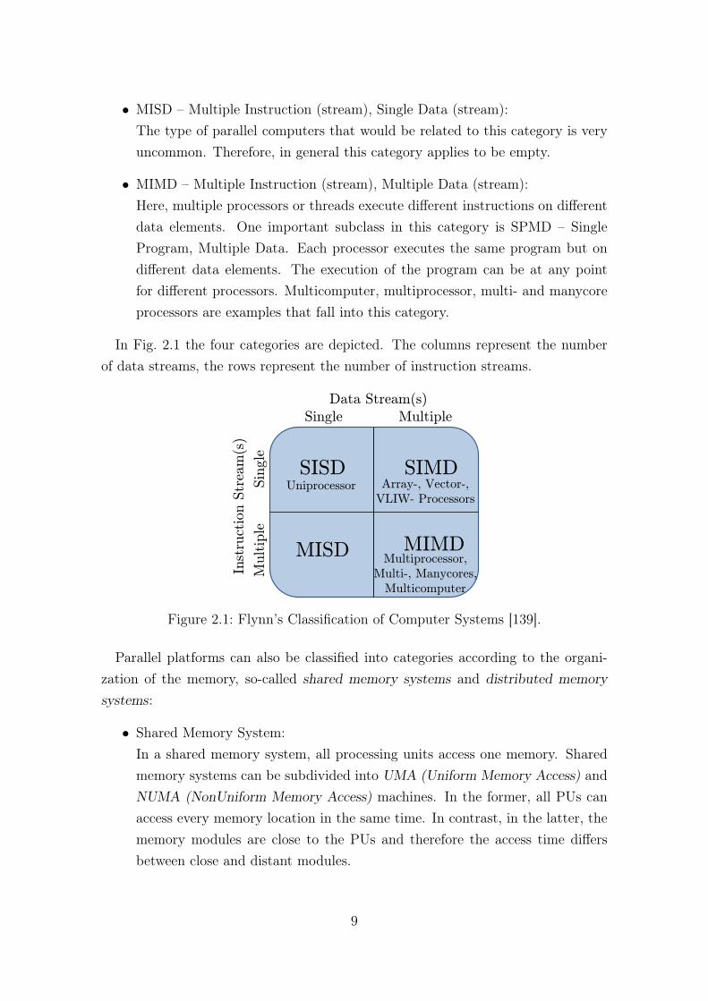
• MISD – Multiple Instruction (stream), Single Data (stream):The type of parallel computers that would be related to this category is veryuncommon. Therefore, in general this category applies to be empty.

• MIMD – Multiple Instruction (stream), Multiple Data (stream):Here, multiple processors or threads execute different instructions on differentdata elements. One important subclass in this category is SPMD – SingleProgram, Multiple Data. Each processor executes the same program but ondifferent data elements. The execution of the program can be at any pointfor different processors. Multicomputer, multiprocessor, multi- and manycoreprocessors are examples that fall into this category.

In Fig. 2.1 the four categories are depicted. The columns represent the numberof data streams, the rows represent the number of instruction streams.

SISD SIMD

MISD MIMD

Data Stream(s)

Inst

ruct

ion S

trea

m(s

)

Single Multiple

Multip

le

S

ingle

Uniprocessor Array-, Vector-,

VLIW- Processors

Multiprocessor,

Multi-, Manycores,

Multicomputer

Figure 2.1: Flynn’s Classification of Computer Systems [139].

Parallel platforms can also be classified into categories according to the organi-zation of the memory, so-called shared memory systems and distributed memorysystems:

• Shared Memory System:In a shared memory system, all processing units access one memory. Sharedmemory systems can be subdivided into UMA (Uniform Memory Access) andNUMA (NonUniform Memory Access) machines. In the former, all PUs canaccess every memory location in the same time. In contrast, in the latter, thememory modules are close to the PUs and therefore the access time differsbetween close and distant modules.

9

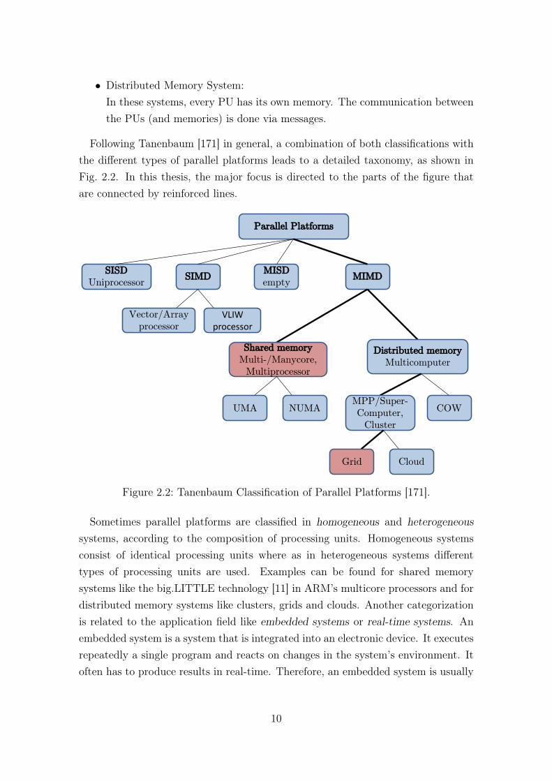
• Distributed Memory System:In these systems, every PU has its own memory. The communication betweenthe PUs (and memories) is done via messages.

Following Tanenbaum [171] in general, a combination of both classifications withthe different types of parallel platforms leads to a detailed taxonomy, as shown inFig. 2.2. In this thesis, the major focus is directed to the parts of the figure thatare connected by reinforced lines.

Parallel Platforms

SISD

Uniprocessor SIMD

MISD

empty MIMD

Vector/Array

processor

VLIW processor

Shared memory

Multi-/Manycore,

Multiprocessor

Distributed memory

Multicomputer

UMA NUMA MPP/Super-

Computer,

Cluster

COW

Grid Cloud

Figure 2.2: Tanenbaum Classification of Parallel Platforms [171].

Sometimes parallel platforms are classified in homogeneous and heterogeneoussystems, according to the composition of processing units. Homogeneous systemsconsist of identical processing units where as in heterogeneous systems differenttypes of processing units are used. Examples can be found for shared memorysystems like the big.LITTLE technology [11] in ARM’s multicore processors and fordistributed memory systems like clusters, grids and clouds. Another categorizationis related to the application field like embedded systems or real-time systems. Anembedded system is a system that is integrated into an electronic device. It executesrepeatedly a single program and reacts on changes in the system’s environment. Itoften has to produce results in real-time. Therefore, an embedded system is usually

10

a real-time system [179]. A major characteristic of a real-time system in comparisonto a non-real-time system is the time constraint. Each program (part) in a real-time system usually has a release time at which the program becomes availableand also a deadline, at which the completion of the program execution must beguaranteed. Thus, not only the logical correctness of an execution is important, butalso the time frame for the execution has to be met. Real-time systems are typicallysubdivided into hard and soft real-time systems. In a hard real-time system, afailure occurs when any deadline is not met, i.e. all deadlines are guaranteed to bemet. For example, the brake control system of a vehicle must be a hard real-timesystem, as an execution delay can lead to life-critical situations. In contrast, in softreal-time systems, a completion of the execution within the deadline is desired butan exceeded deadline does not directly lead to a failure. In image processing forexample, a delayed completion of an image leads to a lower quality but does notcause a life-critical situation [118].

2.2 Parallel Applications

Many real-world situations are complex and massively parallel, e.g. simulating cli-mate changes, rush hour traffics and planetary movements or modeling vehicle con-structions and forecasting the weather [22]. Numerous other examples exist in allsciences like in mathematics, physics, chemistry, biology, computer science, or eco-nomics. Such complex problems can usually be parallelized and executed onto sev-eral computers, e.g. to speed up the execution or to include more details in a model.The design and implementation of corresponding parallel applications or algorithmsare an important challenge to benefit from the underlying parallel platforms.

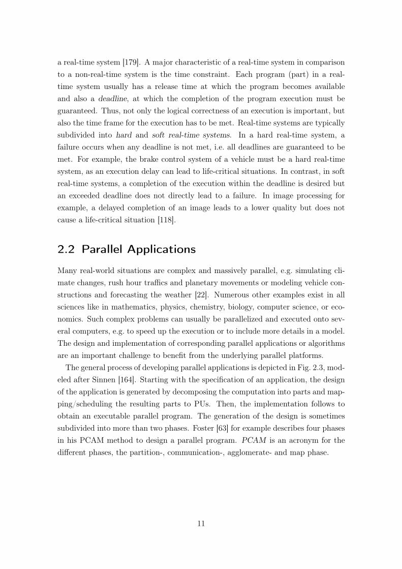
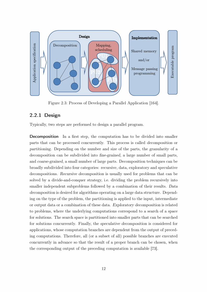
The general process of developing parallel applications is depicted in Fig. 2.3, mod-eled after Sinnen [164]. Starting with the specification of an application, the designof the application is generated by decomposing the computation into parts and map-ping/scheduling the resulting parts to PUs. Then, the implementation follows toobtain an executable parallel program. The generation of the design is sometimessubdivided into more than two phases. Foster [63] for example describes four phasesin his PCAM method to design a parallel program. PCAM is an acronym for thedifferent phases, the partition-, communication-, agglomerate- and map phase.

11

Design

Decomposition Mapping,

scheduling

PU2

PU1

PU3 Applica

tion s

pec

ific

ation

Exec

uta

ble

pro

gra

m

Implementation

Shared memory

and/or

Message passing

programming

Figure 2.3: Process of Developing a Parallel Application [164].

2.2.1 Design

Typically, two steps are performed to design a parallel program.

Decomposition In a first step, the computation has to be divided into smallerparts that can be processed concurrently. This process is called decomposition orpartitioning. Depending on the number and size of the parts, the granularity of adecomposition can be subdivided into fine-grained, a large number of small parts,and coarse-grained, a small number of large parts. Decomposition techniques can bebroadly subdivided into four categories: recursive, data, exploratory and speculativedecompositions. Recursive decomposition is usually used for problems that can besolved by a divide-and-conquer strategy, i.e. dividing the problem recursively intosmaller independent subproblems followed by a combination of their results. Datadecomposition is desired for algorithms operating on a large data structure. Depend-ing on the type of the problem, the partitioning is applied to the input, intermediateor output data or a combination of these data. Exploratory decomposition is relatedto problems, where the underlying computations correspond to a search of a spacefor solutions. The search space is partitioned into smaller parts that can be searchedfor solutions concurrently. Finally, the speculative decomposition is considered forapplications, whose computation branches are dependent from the output of preced-ing computations. Therefore, all (or a subset of all) possible branches are executedconcurrently in advance so that the result of a proper branch can be chosen, whenthe corresponding output of the preceding computation is available [73].

12

Mapping/Scheduling In a second step, the parts have to be assigned to variousprocessors, called mapping and the execution order has to be determined, calledscheduling. While the determination of the execution order can only be accomplishedfor an existing mapping, generally both the spatial (i.e. mapping) and temporalassignment of the parts to PUs is considered, when referring to scheduling [164]. Oneof the major challenges to achieve a good performance is to balance the load overall processors, i.e. scheduling the parts of the computation to processors so that theexecution on all processors finishes at the same time. The parts of the computationcan be independent of each other so that the order of the parts is not important forthe execution. Then, the parts are called jobs. If there are dependencies betweenthe parts, for example the results of parts are used as input for next ones, they arecalled tasks. Next to this, the time for transferring the results has to be considered.While the transfer time on a single core is very small, it grows significantly up whenusing different processors that are interconnected via a LAN or the Internet. Aminimization of the interaction overhead is then additionally striven, to get a goodperformance. Also the job and task flexibility can differ. For example, when jobs ortasks require a fixed number of resources, then they are called rigid. When they canbe parallelized onto several PUs once during the execution, they are called moldable.If the number of PUs can be changed during the execution, the jobs or tasks arecalled malleable [120]. The resulting schedule is then used to create the parallelprogram. In Sect. 2.3 scheduling is described in more detail.

2.2.2 Models

The structure of a parallel application or algorithm is typically given by a parallelalgorithm model that combines various techniques and strategies for the decompo-sition, mapping, scheduling, and for the minimization of the interaction overhead.The most common parallel algorithm models are described in the following [73]:

Task Graph Model Task graphs model a variety of parallel applications. A taskgraph G = (V,E) is typically a DAG (Direct Acyclic Graph) that consists of nodesv ∈ V and edges e ∈ E. The nodes represent the tasks where the workload, e.g.the execution time or number of instructions, is given as a node weight. The edgesrepresent the dependencies between the tasks. Here, a given edge weight describesthe communication costs, usually considered as transfer time. Task graphs can bestatically or dynamically mapped onto PUs.

13

Work Pool Model In a work pool model, the work given as jobs or tasks isdynamically mapped onto PUs. When a PU finishes its execution, a new availablejob or task is assigned to it. The information of the work order is usually storedin a shared list, priority queue, hash table, or in a tree. New tasks or jobs can bedynamically added to the pool.

Master-Slave Model In this model, typically one master-process generates thework and allocates it to the slave-processes. The slave-processes execute the workand send the results back to the master. The work can be generated staticallybefore allocating it to the slave-processes or dynamically, while the slave-processesare busy. In this model, the master-process might become a bottleneck, when thetasks are too small or the slave-processes are too fast so that the slave-processeshave to wait for next tasks and cannot continue the execution directly.

Pipeline or Producer-Consumer Model The pipeline model is based on a chainstructure. The tasks are once allocated onto the PUs. Then, each PU receives someinput data, executes the corresponding task that is assigned to it and generates someoutput data for the next task on the next PU. Thus, a data stream is processed bythis model, where the mapping of the tasks is fixed and only data changes duringthe execution of the whole program. This kind of application structure is sometimescalled stream parallelism.

Data-Parallel Model In the data-parallel model, tasks perform similar operationson different data. Typically, the tasks are mapped and scheduled statically onto thePUs. The execution is sometimes done in different phases, where synchronizationbetween the phases is necessary to receive new data. One example of a data-parallelalgorithm is a matrix multiplication.

2.2.3 Implementation

The implementation of parallel programs is typically based on two paradigms. Asparallel platforms can be classified into shared memory and distributed memoryplatforms (see sect. 2.1), the programming of parallel applications can be subdividedinto shared memory programming and distributed memory programming, the lattercalled message passing.

14

Shared Memory Programming Shared memory programming is typically donewith threads that use a shared address space to communicate to each other. Athread is a lightweight process that consists of a single stream of instructions. Whenusing a shared address space over all threads, an appropriate synchronization of thememory access is necessary to guarantee the correctness of the data. Common APIs(Application Programming Interfaces) for shared memory programming are POSIXthreads (Portable Operating System Interface for uniX) [21] and OpenMP (OpenMulti-Processing) [136].

Message Passing Programming In contrast, in message passing programming,the communication between the processes is explicitly conducted using messages.Each process has its private address space for the data. The communication isbasically done with send and receive operations to transfer data from one process toanother. The MPI (Message Passing Interface) [127] is typically used for this kindof programming.

These two paradigms are related but not restricted to its corresponding class ofparallel platforms. Thus, it is possible to use message passing on a shared mem-ory platform or vice versa shared memory programming on a distributed memoryplatform. But usually, this leads to a lower performance. Often both paradigmsare combined in one program, e.g. when using a multicomputer with multiprocessornodes [73].

2.3 Scheduling1In general, scheduling is the process of assigning activities to resources in time.Examples can be found in various application fields like in production planningand manufacturing, booking systems, or in a simple diary. In computer science,scheduling often describes the spatial and temporal assignment of computationalparts onto different PUs (see Sect. 2.2). The corresponding scheduler that managesthe scheduling process can be realized in either hardware or software. The informa-tion about where and when the parts of the computation should be executed, arethen stored in a schedule [44].Scheduling can be used for several challenges like minimizing the overall comple-

tion time of an application (makespan), for throughput constraints, or minimizing

1The organization of this section is partially based on the presentation in my German diplomathesis [44].

15

the energy consumption of a computer system, to mention only a few. Often acombination of multiple challenges, usually two or three, is desired.

A corresponding scheduling algorithm is typically based on a model that containsat least particulars of the target system architecture and of the parallel applica-tion like explained in Sect. 2.1 and Sect. 2.2. Such particulars for example includewhether the target system is a shared memory or a distributed memory system,whether the system consists of homogeneous or heterogeneous PUs, or how the PUsare interconnected to each other. For the parallel application, particular features areimportant like whether there are dependencies between the parts of the computationor if there exist transfer times or costs. [44]

Scheduling is a NP-complete problem. Finding an optimal solution is typicallyvery compute intensive, especially for problems with a large number of compu-tational parts and PUs. Therefore, instead of finding an optimal solution, oftenapproximation algorithms or heuristics are used to get a satisfying solution that canbe found within an acceptable period of time.

Every year, hundreds of new scheduling approaches for different parallel systemsand applications with various constraints and objective functions are published sothat a summarization of all scheduling variants is impossible. Also several tax-onomies with various focuses are proposed in the literature to categorize the schedul-ing algorithms like in [38], [50], [110], [120], [156] or [173]. However, a completedescription of all taxonomies would go beyond the scope of this thesis. Instead, inthe remaining part of this section a classification of scheduling algorithms for paral-lel applications is described that includes differentiations important for this thesis.Furthermore, exemplary representatives for each class are given or it is sometimesreferred to corresponding techniques in the literature. Finally, key figures are pre-sented to validate different scheduling techniques.

2.3.1 Classification

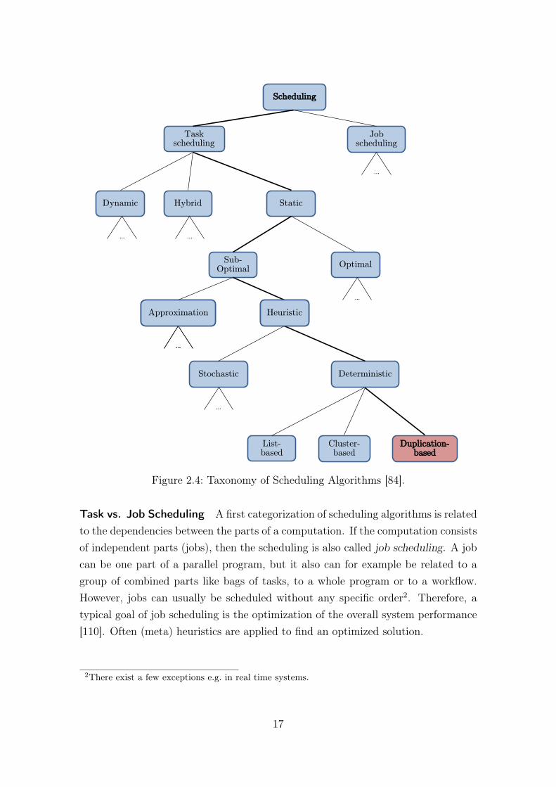
Scheduling algorithms can be subdivided into several classes. In Fig. 2.4 a taxonomyof scheduling algorithms essentially based on [84] is shown. The classes that areconnected by reinforced lines represent the focus of this thesis and, therefore, aredescribed in more detail. For the remaining classes, typical properties are described.A further subdivision of these classes is left out for reasons of clarity.

16

Scheduling

Static Dynamic

Task scheduling

Job scheduling

Hybrid

...

OptimalSub-

Optimal

Heuristic Approximation

...

...

... ...

Cluster- based

List- based

Deterministic Stochastic

Duplication- based

Heuristic

...

...

Approximation

Figure 2.4: Taxonomy of Scheduling Algorithms [84].

Task vs. Job Scheduling A first categorization of scheduling algorithms is relatedto the dependencies between the parts of a computation. If the computation consistsof independent parts (jobs), then the scheduling is also called job scheduling. A jobcan be one part of a parallel program, but it also can for example be related to agroup of combined parts like bags of tasks, to a whole program or to a workflow.However, jobs can usually be scheduled without any specific order2. Therefore, atypical goal of job scheduling is the optimization of the overall system performance[110]. Often (meta) heuristics are applied to find an optimized solution.

2There exist a few exceptions e.g. in real time systems.

17

Braun et al. [34] present eleven different job scheduling heuristics for heteroge-neous distributed computing systems. The scheduling is done statically, i.e. prior toexecution. The goal of the heuristics is to minimize the total execution time.

For computational grids, Subramani et al. [168] present another job schedulingalgorithm. They use distributed scheduling algorithms with multiple simultaneousrequests to improve the performance.

Gao et al. [64] present adaptive job scheduling in grid environments based on twoalgorithms. They use an algorithm for the system-level to decide on which nodea single job should be executed in a shortest time and a genetic algorithm for theapplication-level that is used to minimize the average completion time of all jobs.Two models for a service Grid are designed to predict the completion time of jobs.

In [188], Zaharia et al. present two job scheduling techniques for multi-user mapreduce clusters. With these techniques, they try to improve the data locality andthe throughput. One proposed approach is delay scheduling, where jobs with localdata are chosen first, before also considering jobs with non-local data. The otherapproach is copy-compute splitting, where the jobs are divided into two types (copytasks and compute tasks), according to their operations.

For job scheduling on computational grids, Pooranian et al. [143] present a hybridmeta heuristic algorithm. They combine a genetic algorithm for searching the prob-lem space globally and gravitational emulation for local search. With their approach,the runtime and number of submitted tasks that miss deadlines are decreased.

Shojafar et al. [161] present a meta-heuristic job scheduling approach for cloudenvironments to minimize the makespan. The scheduling algorithm, called FUGE3,is based on a genetic algorithm combined with fuzzy theory to optimize the loadbalancing in terms of execution time and cost.

In [72], Goswami et al. present a deadline stringency based job scheduling ap-proach for computational grids that is based on an already existing so-called NDFS(Nearest Deadline First Served) algorithm. They try to improve the dynamic loadbalancing by simultaneously receiving job requirements and collecting runtime sta-tus informations of the resources for the allocation of the jobs.

Lopes and Menascé [120] propose a current approach to categorize job schedulingalgorithms. They present the trends of job scheduling research for the last decadebased on over 1,000 analyzed job scheduling papers and provide a taxonomy of jobscheduling. They classify the most cited 100 problems with their taxonomy intoten groups, that differ next to others in the used environment and the structure

3The authors omit a long form of the term FUGE.

18

of jobs. Additionally, they give for each group the proposed solutions with typicalproperties.

When there exist dependencies between the parts (tasks), the scheduling is calledtask scheduling. Task scheduling is often done with the help of a task graph thatrepresents the structure of a parallel program (see Sect. 2.3). The information of thetask graph is then used to create an appropriate schedule. Therefore, task schedulingis sometimes called task graph scheduling. A common challenge of task scheduling isthe minimization of the makespan. (Task) Scheduling can further be subdivided bythe time, when the scheduling process is done, into static and dynamic scheduling.

Static vs. Dynamic Static scheduling is done prior to execution, sometimes calledoffline. In contrast, dynamic scheduling is done during the execution, called online.While the static scheduling does not influence the runtime of the correspondingapplication, it cannot react as the dynamic scheduling on unpredictable situationsthat might occur during the execution. However, the calculations for the dynamicscheduling prolong the execution of the parallel application and thus the makespanof the schedule [84][110]. Dynamic scheduling is mainly used for problems, whereno information about the tasks is known prior to execution. Therefore, the goal ofdynamic scheduling is usually Load Balancing.

For example, Ramamritham et al. [151] describe a dynamic task scheduling ap-proach for hard real-time distributed systems. They assume that each node withinthe system has its own scheduler and a set of periodic tasks that are guaranteed tomeet their deadlines. Additionally, aperiodic tasks can arrive at any time on anynode in the system. The scheduler on the corresponding node checks whether thetask can be assigned to that node without violating the deadline constraints. If thetask cannot be allocated suitably on the local node, the scheduler interacts with theschedulers of other nodes by using a bidding scheme to determine on which nodethe task can better be allocated. Then, the task is sent to the corresponding node.

Manimaran and Murthy [125] present another approach for real-time systems.They assume to have a multiprocessor system and aperiodic tasks that can arriveat any time. A dynamic scheduler is used to allocate the tasks onto the processors.Instead of restricting on non-parallelizable tasks, the tasks can be parallelized ontoseveral processors. The scheduler takes advantage of the task parallelization to meetthe deadline constraints.

In [150], Rahman et al. present a dynamic scheduling algorithm for workflow ap-plications on global grids. They extend an already existing scheduling approach

19

for homogeneous systems to include heterogeneous and dynamic environments. Thescheduling is done stepwise by calculating dynamically the critical path in the work-flow task graph and prioritizing tasks to respect the dependencies.

For grid computing systems, Zhang et al. [192] present a dynamic task schedulingalgorithm. They extend a two phase algorithm that originally is used for staticscheduling. The algorithm first selects the tasks and then the processors to allocatethe tasks. The tasks are related to levels, so that equal levels indicate independenttasks, otherwise there exist dependencies between the tasks.

Amalarethinam et al. [8] present a DAG based dynamic task scheduling algo-rithm called DYTAS (DYnamic TAsk Scheduling) for multiprocessor systems. Thescheduling is done by using several different task queues: One initial queue, a dis-patch and completed queue, and individual processor task queues. After starting thescheduler, the tasks are ordered by their dependencies. Then, the processor queueis dynamically chosen, where the next task can finish at the earliest time. When theprocessor queues become empty, the algorithm stops.

In contrast, static scheduling can only be done, when information about the tasksand there dependencies are known in advance. Sometimes also a hybrid variant isused, i.e. a combination of static and dynamic scheduling like in [9], [116], [133] or[191]. (Static) scheduling can further be subdivided by the quality of the solutions,into optimal and sub-optimal scheduling.

Optimal vs. Sub-optimal Most of the scheduling problems for parallel applica-tions are NP-hard [164]. This means that no polynomial-time algorithm exists tosolve the problems optimally (unless P = NP). While for small instances of thoseproblems optimal solutions might be found within an acceptable period of time, itis infeasible for larger instances.

Wang et al. [181] present an optimal task scheduling approach for streaming ap-plications on MP-SoCs. They describe the problem as an ILP (Integer Linear Pro-gramming) formulation. The objective is to minimize the makespan by avoidinginter-core communication overhead. Furthermore, they also try to reduce the en-ergy consumption by using DVS (Dynamic Voltage Scaling).

Shioda et al. [160] present an optimal task scheduling algorithm for parallel pro-cessing. They propose an ILP formulation, where the objective is the minimizationof the makespan. With their approach, they also try to minimize idle times.

In [85], Hönig and Schiffmann present a fast optimal task graph scheduling ap-proach for homogeneous computing systems. They use a parallel variant of an

20

informed search algorithm based on an IDA*-algorithm (Iterative Deepening A*),which is a memory-saving derivative of the well known A*-algorithm [78]. The ob-jective is to optimize the makespan. Their approach is not restricted to task graphproblems with a small number of tasks, but complex task graphs can be computedby their IDA*-algorithm as well.

Cho et al. [42] propose an optimal real-time scheduling algorithm for multipro-cessors called LLREF (Largest Local Remaining Execution First). The algorithm isbased on a fluid scheduling model, i.e. each task executes at a constant rate at alltimes. To describe the task execution behavior on multiprocessors, the algorithmuses time and local execution time domain planes (T-L planes). They show thatscheduling for multiprocessors can be viewed as repeatedly occurring T-L planes,where a feasible solution for a single T-L plane results in an optimal schedule.

Next to optimal algorithms, two sub-optimal approaches are usually used to findat least optimized solutions in a short period of time. The first one is to use approx-imation algorithms to find an approximation of the optimal solution, the second oneis to use heuristics that make their decisions based on predefined assumptions.

Approximation vs. Heuristic In approximation algorithms, the objective to findan optimal solution is slightly relaxed for finding solutions that are close to theoptimal. However, instead of searching the whole solution space to find an optimalone, the algorithm stops, when a solution is found that is rated as "good" enough.Typically a factor p is given that describes the guarantee on how close the solutionto the optimal at least will be. Therefore, these algorithms are sometimes calledp-approximation algorithms.Giroudeau et al. [69] present in their work an approximation for precedence con-

strained scheduling problems with large communication delays. They focus on mul-tiprocessor systems and try to minimize the makespan. A lower bound for the per-formance of an approximation algorithm is given by using a variant of the problem3SAT (3-SATisfiability) and an impossibility theorem. They propose a polynomial-time algorithm with a performance ratio of 2(c+1)

3with c ≤ 2, where c denotes the

communication delay between two tasks.Chen and Chu [40] present another approach for scheduling malleable tasks. They

assume that the processing time of a malleable task is non-increasing and the worknon-decreasing in the number of processors. Their polynomial-time approximationalgorithm can yield an approximation ratio of 3.4142 and for strictly decreasingprocessing times in the number of processors the ratio is 2.9549.

21

For scheduling malleable tasks under precedence constraints, Lepère et al. [114]present an approximation algorithm. They demonstrate a close relationship to theallotment problem and design a polynomial time approximation algorithm with aperformance guarantee close to 2.61803 for different special cases and with a guar-antee of 5.23606 for the general case.

In [87], Hunold presents a scheduling algorithm for moldable tasks on multipro-cessors. The objective is the minimization of the makespan. He tries to reduce thecritical path while keeping the overall work small by introducing a relative runtimethreshold that defines the minimum runtime improvement of a larger allotment.

For scheduling malleable tasks under general precedence constraints, Jansen andZhang [94] present an approximation algorithm. They developed an improved ver-sion of their previous approximation algorithm with a ratio of 4.730598.

Günther et al. [74] present in their work a scheduling and packing approach formalleable tasks with precedence constraints of bounded width.

In contrast, heuristics make their decisions based on predefined assumptions, i.e.a heuristic follows fixed rules that are defined based on experiences with the treatedproblem type. Therefore, heuristics are usually very fast in finding a solution, butthere is no guarantee to find an optimal or at least a near to the optimal solution.The results of a heuristic are usually compared to results of other heuristics or tooptimal solutions to get informations about the quality of the heuristic. Heuristicscan further be subdivided into stochastic and deterministic methods.

Stochastic vs. Deterministic Stochastic methods try to find a possibly optimalsolution with the help of random-based algorithms. During the runtime, either ex-actly one solution can be considered or several alternative solutions [44]. Techniquesthat only consider one solution are Tabu Search [70] and Simulated Annealing [158].Representatives for considering several solutions are Genetic Algorithms [62] andSwarm Algorithms [137].

Blum [29] presents in his work an introduction and recent trends of a swarmalgorithm, the so-called ACO algorithm (Ant Colony Optimization). In the nature,ants produce messenger substances, so-called pheromones, to find a way to some foodand back to their colony. Over time, a shorter path results in a more dominant traceand the probability increases that other ants will also follow this trace. This behaviorleads to an optimized solution. In the ACO algorithm, the ants are represented byagents and the pheromones by values depending on the quality of a solution. Thevalues are then stored in a so-called pheromones-matrix.

22

Singh [162] for example presents a genetic algorithm for task scheduling in parallelsystems. He considers dependencies between tasks and assumes to have no commu-nication costs. As target system, he uses multiprocessor systems with heterogeneousprocessors.

For scheduling tasks with precedence constraints, Omara and Arafa [135] presenttwo genetic algorithms. They try to improve the performance of the genetic algo-rithms by adding heuristic principles. For the first algorithm, two fitness functionsare used in a row with the objectives to minimize the makespan and to balance theload. The second algorithm is extended by a duplication-based technique to reducethe communication overhead.

Daoud and Kharma [48] present another genetic algorithm for task schedulingin heterogeneous distributed systems. They use a customized genetic algorithm toproduce optimized schedules. The algorithm starts with a scheduling heuristic forthe initial population. The schedule is then located at an approximate area in thesearch space that is used for the genetic algorithm to improve the schedule.

Porto and Ribeiro [144] present a tabu search approach for heterogeneous pro-cessors. They consider task scheduling and show that their approach results insolutions that are improved by up to 30 percent compared to the most appropriatealgorithms.

Deterministic methods, in contrast, can further be classified into list-based, cluster-based and duplication-based algorithms.

List- vs. Cluster- vs. Duplication-based In list-based method, nodes (tasks) areordered with priorities in a scheduling list. To prioritize tasks, different approachesare proposed like CP (Critical Path), HLF (Highest Level First), LP (Longest Path)or LPT (Longest Processing Time). List scheduling can be done statically or dy-namically. In the static variant, the tasks are obtained prior to execution from thebeginning of the list and assigned to PUs where they can earliest start. However,the dynamic variant consists of three steps: prioritize unscheduled tasks, select thetask with the highest priority and allocate it to a PU. After each allocation, thescheduling list is rearranged. The priorities are assigned with the help of task at-tributes. The most common are the so-called t-level (top level) and b-level (bottomlevel). The t-level is the longest path between an entry node and the current node,by considering the node and edge weights. The b-level is the longest path betweenthe current node and an exit node and is bounded by the critical path [110].

23

Adam et al. [2] for example present list-based approaches. They propose aHLFET-method (Highest Level First with Estimated Times). In this method, a static b-level,so-called sb-level, is used to prioritize the tasks in a scheduling list. In contrast tothe common b-level, the sb-level only considers the node weights. After prioritizingthe tasks, they are allocated to the PUs by a greedy mapper. A greedy mapperassigns each task to the PU that can finish the execution of a task first.

Kasahara and Narita [101] present an enhanced version of the HLFET-method.They propose a so-called CP/MISF-method (Critical Path/ Most Immediate Succes-sors First). In contrast to the HLFET-method, tasks with same priorities are sortedin the scheduling list by the number of direct successor tasks and not randomly.

In [49], Daoud and Kharma present a list-based algorithm for heterogeneous dis-tributed systems. They consider dependent tasks with communication costs andtry to minimize the total execution time. The so-called LDCP (Longest DynamicCritical Path) algorithm consists of three phases. In each scheduling step, a taskselection, processor selection and a status update is done. The status update is nec-essary, because only when a task is assigned to a processor, the computation timeis known and communication costs of succeeding tasks can be updated.

Macey and Zomaya [124] present a performance evaluation of list scheduling algo-rithms. They compare the performance of different popular list scheduling heuristicslike HLFET and others. Their results demonstrate the inadequacies of the list-basedheuristics in communication-intensive cases.

For heterogeneous target systems, Bjørn-Jørgensen and Madsen [27] present an-other approach. They propose an algorithm called HCP-algorithm (HeterogeneousCritical Path) that considers both concurrently the interprocessor communicationand the heterogeneity of the target system.In [165], Sllame and Drabek present a list-based scheduling algorithm for high-level

synthesis. This algorithm produces near-optimal schedules by including informationextracted from a data flow graph (like the number of successors and predecessors)into the priority functions of the scheduler.In cluster-based task scheduling, the makespan of a schedule is optimized by

combining tasks suitably to reduce communication costs. Therefore, the tasks arecombined to so-called clusters that are merged together until no further reductionof the makespan is possible. In general, there are two different methods. The UNC-method (Unbounded Number of Clusters) and the BNP-method (Bounded Numberof Processors). In the former method, an unlimited number of processors is assumedto get a high reduction of the makespan. A post processing step is then necessary

24

to map the clusters onto the available processors. In contrast, in the BNP-method,the existing target system is directly considered so that no post processing step isrequired [84][110].

For an unbounded number of processors, Yang and Gerasoulis [186] present acluster-based algorithm. In the so-called DSC-algorithm (Dominant Sequence Clus-tering), a task is assigned to a cluster when the longest path between an entry taskand the current task is minimized by saving the communication costs. Therefore,the critical path of the partial schedule (called dominant sequence) is used. If thetask is not on the critical path, it must be proved whether the assignment leadsto a worsening of tasks with a higher priority. Is it not possible to assign a taskto an existing cluster, the task is assigned to a new cluster. Gerasoulis and Yangpresent in a further work a comparison of clustering heuristics for scheduling DAGson multiprocessors [68].

Cirou and Jeannot [46] propose an approach for heterogeneous systems. Theypresent a multi-step scheduling algorithm called triplet. Initially, the tasks arecombined to clusters. Then, platforms with same characteristics are grouped toworkstation clusters. Finally, the clusters are mapped to the workstation clusters.

In duplication-based scheduling, so-called TDB (Task Duplication-Based), also areduction of the communication costs is desired. In contrast to the cluster-basedscheduling, the tasks are replicated. If dependent tasks are on the same PU, nocommunication costs are needed. If a task has several descendants, only duplicatescan avoid communication costs (and serialization). Some algorithms replicate onlydirect predecessor tasks, others in turn all predecessors. The replicated tasks (dupli-cates) are then mapped onto different PUs. If a successor task is placed on the samePU like the duplicate, the communication costs between them can be neglected [44].

Papadimitriou and Yannakakis [138] present a duplication-based algorithm calledPY -algorithm (Papadimitriou Yannakakis). The tasks are assigned to PUs by usinga so-called e-value that represents the earliest start time of a task. If a task can onlybe started after the e-value because of dependencies, the predecessors are duplicatedand placed onto the same PU like the considered task. Thus, the communicationcosts are eliminated and the makespan is reduced.

Bozdag et al. [33] present a task duplication-based algorithm called DUPS (Dup-lication-based scheduling Using Partial Schedules). The algorithm consists of twophases: one for minimizing the schedule length by using partial schedules and onefor reducing the number of required processors by merging and eliminating theschedules. Duplicates are created in the first phase to construct partial schedules.

25

In [32], Bozdag et al. present a further duplication-based algorithm called DBUS(Duplication-based Bottom-Up Scheduling) for heterogeneous environments.In [109], Kwok presents a task duplication-based approach for heterogeneous clus-

ters. To minimize the makespan, tasks on the critical path are replicated onto fastermachines.

Ahmad et al. [4] present a comparison of different algorithms for task graphs onparallel processors. Next to task duplication-based algorithms, list- and cluster-based algorithms are considered.

Kaur and Kaur [103], and Gupta et al. [75] present a review of duplication-basedscheduling algorithms.

Often a combination of list-, duplication- and cluster-based methods is used. Kru-atrachue et al. [108] and Bansal et al. [19] present combinations of duplication- andlist-based scheduling algorithms.

2.3.2 Performance and Cost Metrics

In order to make a statement about the quality of a scheduling algorithm, variousfactors can be considered. Depending on the application field and the resulting typeof scheduling, different factors are important, e.g. the performance, scalability, costor throughput. Several metrics are proposed in the literature like in [36], [60], [90],[102] and [107] to validate the quality and thus to make a scheduling algorithmcomparable against existing ones. In the following, necessary performance and costmetrics for this work are described.

Makespan Themakespan or schedule length of a schedule is the overall completiontime CT of a schedule. It describes the length between the starting point of anexecution and the ending point. In a parallel program, where the tasks of theprogram are executed on different PUs, the makespan is the length between theearliest starting task of the schedule execution and the latest ending task over allPUs [39]. The makespan can be described by equation 2.1, where i is the task index:

Makespan = max(CTi), (2.1)

Speedup A common performance metric for scheduling algorithms is the speedup.Important for the speedup is the schedule length (i.e. the makespan of a schedule).The speedup of a parallel program and thus of a schedule is then the ratio between

26

the sequential schedule length SLseq and the parallel schedule length SLpara [73][184].It can be described by equation 2.2:

Speedup =SLseqSLpara

(2.2)

In the literature, different types of speedups like absolute or relative speedup aredescribed, depending on different assumptions to the sequential schedule length. Inthis work, SLseq is defined as the sum of all task execution times.

Efficiency The efficiency of a scheduling algorithm is defined by the ratio betweenthe speedup and the number of PUs. Thus, it represents the average usage rate ofall PUs of the system during the execution of a schedule [73].

Efficiency =Speedup#PUs

(2.3)

Scheduling Time A common cost metric for scheduling is the scheduling time. Itrepresents the running time of an algorithm to find a resulting schedule [174].

2.4 Fault Tolerance4A fault is the cause of an error. Examples are a transistor defect or an incorrectline of program code. An error is the visible effect of a fault like a wrong behaviorof an application due to the incorrect code line. Faults can occur at any time ina computer system. Some faults have a major effect on the behavior of a system,e.g. a damaged or overheated processor leads to a failure, while others affect thesystem only marginally, e.g. a wrong presentation of some results in an application[51][167].

Therefore, it is important to classify faults to handle them appropriately [52]. Inaddition, the application field of a system is important for the handling of a fault.For example in a medical or industrial field a faulty system or at least a faultycomponent (in hardware or software) leads to high costs in sense of time, moneyup to life-critical situations. In such application fields, a correct system behavior ismandatory.

4The organization of this section is partially based on the presentation in my German diplomathesis [44].

27

In general, there exist two approaches for the handling of faults, the fault avoid-ance and the fault tolerance. The fault avoidance is typically used in the planningand development phase of hardware and software in order to avoid faults directly inadvance, e.g. with additional tests and systematic designs. In contrast, fault toler-ance is used to detect and treat faults after they have occurred, so that the systemstill functions correctly (despite faults) [51][52][167].

In parallel systems with a large number of PUs like in grids or manycores, wherea failure of a PU can occur during the execution of a scheduled parallel program,fault tolerance is very important. In such systems, unexpected faults often occurduring operation, e.g. failures due to hardware, software and connection faults ordue to the shutdown of PUs by their owner (in a grid), so that a fault avoidanceis impossible in advance. In addition, the probability of a fault increases with thenumber of PUs [51]. Therefore, several approaches for fault-tolerant scheduling arepresented in the literature.

Whenever fault tolerance is used, some kind of redundancy is necessary, e.g. by in-cluding additional components in hard- or software, by supporting special functions,or by using extra time for fault-tolerant techniques. Basically, redundancy describesthe existence of additional resources that are dispensable for a correct functioningof a system in general, i.e. in a fault-free case [30][52]. To develop and evaluatefault-tolerant techniques, failure models are often used. A failure model describesthe assumptions about the system in use and the tolerable faults that should besupported by the system [66].

In this section, firstly a classification of faults is given and different failure modelsare explained. Secondly, fault-tolerant scheduling and corresponding approaches arepresented. Finally, difficulties in real implementations by using MPI are described.

2.4.1 Classification of Faults

There exist different faults that can occur in a computer system. Faults are usuallycategorized into several classes according to their properties. These classes can beused to develop fault-tolerant techniques for a group of faults. In the following, themost common categories are described. A first classification can be done accordingto the cause of a fault into design, production and operation faults [51][52]:

• Design Fault:A design fault is caused in the planning and designing phase of a systemby a wrong specification, documentation or mistakes in the implementation.

28

For example an incorrect algorithm or architectural specifications that do notmatch the requirements for the application field of a system.

• Production Fault:Faults that are caused in the manufacturing of a system are called productionfaults. For example inaccuracies in the fabrication process of hardware likeprocessor chips or faults from the replication process of software, when copyingan application to another medium.

• Operation Fault:Operation faults are caused during the runtime of a system, i.e. the systemwas initially faultless. For example wear-out and aging failures, mistakes inthe use of programs or a wrong handling in the maintenance.

Faults can also be subdivided into software and hardware faults [51]:

• Hardware Fault:A hardware fault is caused by physical defects in the system or component.For example broken pins of a processor, defect memory cells in a RAM module,or short-circuits.

• Software Fault:Faults that are caused in the software are related to this category. The softwarecan be for example a standalone application, an operating system or driversfor hardware components. Most software faults are caused by implementationmistakes in the design phase or due to incorrect updates.

Another differentiation of faults is based on the duration of a fault into temporary(transient and intermittent) or permanent faults [51]:

• Temporary Fault:Faults that occur for a short time during the life cycle of a hard- or softwareare called temporary faults. If a fault occurs only once it is also called atransient fault. These faults typically arise due to external influences likecosmic rays or electrical power drops. If a fault occurs periodically, it is alsocalled intermittent fault. These faults are usually based on implementationmistakes or unexpected operation conditions.

• Permanent Fault:A permanent fault exists until the state of the corresponding hard- or softwareis changed by restarting, changing or replacing the component.

29

2.4.2 Failure Models

In the literature, several failure models are presented, e.g. in [51], [66], [166] and[176]. Therefore, only the most common are described in the following [66]:

• Fail-stop Model:In this model, a failure of a PU can occur at any time. The information abouta failure is distributed to the other PUs automatically, as the faulty PU cannotsend or receive messages anymore. A recovery of the faulty PU is impossible.

• Crash Model:The crash model is similar to the fail-stop model. But the information abouta failure is not distributed automatically. The remaining PUs only get theinformation about a failure, when they do not receive any response of thefaulty PU to a request within a time frame.

• Crash Recovery Model:In contrast to the crash model, a faulty PU can be recovered in this modelafter a while.

2.4.3 Fault-tolerant Scheduling

In fault-tolerant scheduling, the most common software techniques are checkpointingand replication. Checkpointing is a backward error recovery technique. With thistechnique the system state is saved periodically in a checkpoint. When a faultoccurs, the faulty system state is replaced by the last fault-free checkpoint and theexecution is continued [148].

In replication, the fault tolerance is achieved by copying parts of an applicationonto other PUs. In case of a failure of one PU, either the original or the copyfinishes. The execution of the application can continue. This technique can besubdivided into active and passive replication. In active replication, multiple copiesof a program part are mapped onto different PUs and executed in parallel. Inthis case, a fixed number of failures is tolerated. Passive replication uses only onebackup copy per program part. The backup copy is not executed in parallel withthe original. Instead, it only runs if the original fails [16].

If only one copy is used in general, replication is also called duplication and thecopy of each program part is called a duplicate. This scheduling approach is then

30

related to task duplication-based scheduling (see Sect. 2.3.1). Sometimes hybridtechniques that combine checkpointing and replication are used.

As a fault or failure can only be survived or not, often the (performance) over-head in both the fault-free and the fault case are used to evaluate the fault-tolerantscheduling approaches. The overhead is the difference between the makespan with-out any fault-tolerant aspects m and the makespan with fault tolerance includedmft in percent and can be expressed by [44][53]:

Overhead =mft −m

m· 100. (2.4)

In this equation, no difference between the fault-free and fault case is considered.Therefore, the relation of the overhead to the corresponding case is always specifiedin this thesis, if it is not clear in the context.

Fault-tolerant scheduling has been studied over decades, thus numerous approachesexist in the literature for both checkpointing and replication. Therefore, only someexamples are presented in the following:

Approaches using Checkpointing Poola et al. [141] present a fault-tolerant schedul-ing approach for workflows in cloud computing. They minimize the execution costsby using different cloud instances for a workflow and tolerate failures by includingcheckpoints.

In [17], Balpande and Shrawankar present a fault-tolerant job scheduling approachfor computational grids. They propose two different checkpointing schemes. Theso-called ABSC (Algorithm Based on System Checkpointing) scheme is based on agenetic algorithm and used for non-intensive applications. In the so-called ABAC(Algorithm Based on Application Checkpointing) scheme a computational intensiveapplication is extended to make and store checkpoints.

For computational workflows, Aupy et al. [13] present another approach. Theypropose a polynomial-time optimal algorithm for fork DAGs. A fork DAG is a taskgraph with one entry task, n exit tasks and n edges from the entry task to eachexit task. Their goal is to minimize the expected execution time for a workflow bymaking decisions about the execution order of tasks and when to checkpoint.

Prashar et al. [145] present a fault-tolerant approach in grid computing by combin-ing checkpointing with an ACO algorithm. The ACO algorithm is used to balancethe load over nodes in a grid. Checkpointing is considered to handle faults of re-sources.

31

For computational grids, Babu and Rao [14] present an automated checkpointingstrategy. They assume a heterogeneous system and independent jobs to be sched-uled. MPI and BLCR (Berkeley Lab Checkpoint/Restart), a package to supportinteractive checkpointing on MPI applications, is used.

In [163], Singh presents a fault-tolerant scheduling algorithm for grids with check-pointing. He considers the failure rate and the computational capacity of resourcesto minimize the makespan and cost of a schedule.

Nazir et al. [132] present an adaptive checkpointing strategy for economy basedgrids. They propose a fault index of grid resources that is dynamically updatedbased on successful or unsuccessful execution of tasks. The fault index is used forthe intensity of checkpointing, i.e. the checkpoint interval.

Further approaches using checkpointing can be found e.g. in [65], [146] or [149].

Approaches using Replication Litke et al. [117] present an efficient static fault-tolerant task replication approach for mobile grid environments. They considermultiple replications per task depending on the probability of a failure. The goal isto maximize the utilization of the grid resources.

For multiprocessors, Jun et al. [98] present another fault-tolerant approach. Theypropose two different scheduling methods for both active and passive replication.The first method is based on an ILP formulation to find optimal schedules, thesecond one is a heuristic algorithm that can achieve close to optimal solutions.

In [177], Tsuchiya et al. present a dynamic fault-tolerant replication-based schedul-ing technique for real-time multiprocessors. They assume aperiodic tasks and con-sider one copy per task. The copy is divided into two parts: one part that can beexecuted simultaneously to the original task (so-called redundant part) and anotherpart (so-called backup part) that runs after the original task. Thus, the backup parthas only to be executed when the original task fails.

Ahn et al. [5] present a fault-tolerant scheduling approach for hard real-time sys-tems. They use passive replication and also consider aperiodic tasks. In contrastto Tsuchiya et al., an overlapping of an original task and a copy of another task isallowed in their dynamic scheduling heuristic.

In [1], Abawajy presents a dynamic fault-tolerant scheduling approach for gridsystems called DFTS (Distributed Fault-Tolerant Scheduling). He assumes a fail-stop model and a certain number of replicas given by the user.

In [183], Wensley et al. present a fault-tolerant approach for aircraft control calledSIFT (Software Implemented Fault Tolerance). They use triplication of tasks to

32

tolerate a single failure of a processing unit or bus. Iterative tasks are assumed andredundantly executed. Consequently, the results of each iteration are initially votedbefore they are used.

Poola et al. [142] present a fault-tolerant approach for workflows in cloud envi-ronments. They propose a just-in-time scheduling heuristic that uses replication toutilize different pricing models offered by clouds.

Further investigations on fault-tolerant scheduling with replication can be foundin [25], [31] and [182].

Combinations Nandagopal and Uthariaraj [130] present a combined fault-tolerantapproach for computational grids. They use checkpointing to tolerate failures andreplication to increase the availability of checkpoints.

Nazir and Khan [131] present a fault-tolerant job scheduling approach for compu-tational grids. They consider checkpointing and replication. In their approach theintensity of both is dependent on the fault occurrence history of a resource.

In [43], Chtepen et al. present an efficient fault-tolerant approach that combinescheckpointing with replication. They propose to dynamically switch between bothtechniques according to the runtime information and system load. Next to theirproposed algorithm several checkpointing and replication approaches are presentedthat dynamically adapt the checkpointing interval and the number of replicas.

Further combined fault-tolerant approaches can be found in [15] and [187].

2.4.4 Fault Tolerance in MPI

We consider a fault-tolerant MPI-application that can survive a failure. In thebasic version, MPI does not support fault tolerance. When an MPI-process fails forsome reason, the typical behavior of MPI is to abort the whole application, i.e. allremaining MPI-processes. This behavior can be changed by using an additional flag(-gmca orte_abort_on _non_zero_status 0), when starting the MPI-applicationwith mpirun *. The execution of an MPI-application is then continued. But in thiscase, no further collective functions can be used, as the standard intra-communicatoris MPI_COMM_WORLD, that includes all started MPI-processes and is staticduring the runtime. In every MPI-application the parallel part must be startedand ended with the collective functions MPI_Init() and MPI_finalize() that arerelated to the standard intra-communicator. If an MPI-process fails within thispart, the MPI_finalize() function leads to an endless loop, because the failed

33

MPI-process did not reach this function. One option to avoid the collective functionin the end of the MPI-application is to use an explicit call of MPI_Abort(Comm)

for each remaining process. But the typical behavior of MPI is to abort the wholeMPI-application when the first MPI_Abort(Comm) is executed. Also in this case, theapplication terminates with an error message. Thus, there exist several difficultieswhy MPI in its standard version is unsuitable to execute fault-tolerant applications.

Fagg and Dongarra [58] present an approach to control the behavior of MPI withinan application. The so-called FT-MPI (Fault-Tolerant MPI) is an extension of MPI,that supports different failure modes for checkpointing and replication techniquesby including semantics into MPI. It is used in combination with a core librarycalled HARNESS (Heterogeneous Adaptive Reconfigurable Networked SyStem), tobuild necessary services for FT-MPI. The main feature of FT-MPI is to handlefailures by modifying the standard communicator of MPI. Different options aregiven, like shrinking the communicator size and reordering the ranking of MPI-processes or to fill-up the MPI-application with new MPI-processes and to rebuildthe communicator.

Bland [28] presents another approach called ULFM-MPI (User Level Failure Mit-igation MPI). It is based on Open MPI and also includes several semantics andconstructs, to control the behavior of MPI during runtime. In contrast to FT-MPI,an additional runtime system like HARNESS is unnecessary and the constructs al-low a more detailed behavior control. ULFM-MPI can be interpreted as a successorvariant of FT-MPI, that is built by a working group of the MPI forum with the goalto be included in the MPI standards in the future.

2.5 Energy Efficiency

In computer systems like manycores or grids that are typically used for computa-tional intensive applications, the processor (core) is one of the most power consumingcomponents. Several hardware and software mechanisms have been integrated intothe systems to reduce the power consumption and therefore the energy consump-tion of those components, and finally for the entire system. Today, most processorssupport different frequency and voltage levels as well as multiple sleep states. Oper-ating systems must provide appropriate software energy management functions, touse such hardware features of a processor. A common standard for these functions isgiven by the ACPI (Advanced Configuration and Power Interface) [82]. In addition,the operating system is typically responsible for adequately utilizing these functions.

34

Especially in grids and manycores, where the PUs are controlled by separateoperating systems, an efficient utilization of the energy management functions isimpossible because the operating systems are not aware about the parallel applica-tion to be executed. In such a case, the scheduler or the underlying runtime systemmust support corresponding features. Therefore, numerous scheduling approachesare proposed in the literature, which consider energy efficiency.

Typically, energy efficiency can either be described as using less energy to providethe same amount of service or as using the same amount of energy to provide anincreased service [35][89]. Both definitions are correct depending on the perspective.In this thesis, the first definition is considered and corresponding energy-efficientscheduling heuristics and strategies are presented in Chap. 4.

To provide energy-efficient scheduling, i.e. reducing the energy consumption for atask or schedule, a prediction of the energy consumption is necessary. Therefore, anappropriate power model for the system in use must be defined.

In the remainder of this section, firstly energy consumption is defined and powerconsumption explained. Secondly, typical aspects of modeling the power consump-tion of a processor (core) are described. Then, energy-efficient scheduling and cor-responding approaches are presented. Finally, limitations and issues in real systemsare described.

2.5.1 Energy Consumption

The energy consumption E for a certain time span t = [t1; t2] is the power consump-tion P integrated over time and is expressed by:

E =

∫ t2

t1

P (t)dt (2.5)

If P is constant over time, then this reduces to E = P · (t2 − t1). The energy istypically measured in J (Joule), which corresponds to Ws (Watt-second).

The power consumption (measured in W (Watt)) of a processor (core) is subdi-vided into a static part Pstatic that is frequency independent and a dynamic partPdynamic, which depends on both the frequency and voltage. The total power con-sumption is then the sum of the static and dynamic power consumption:

P = Pstatic + Pdynamic (2.6)

35

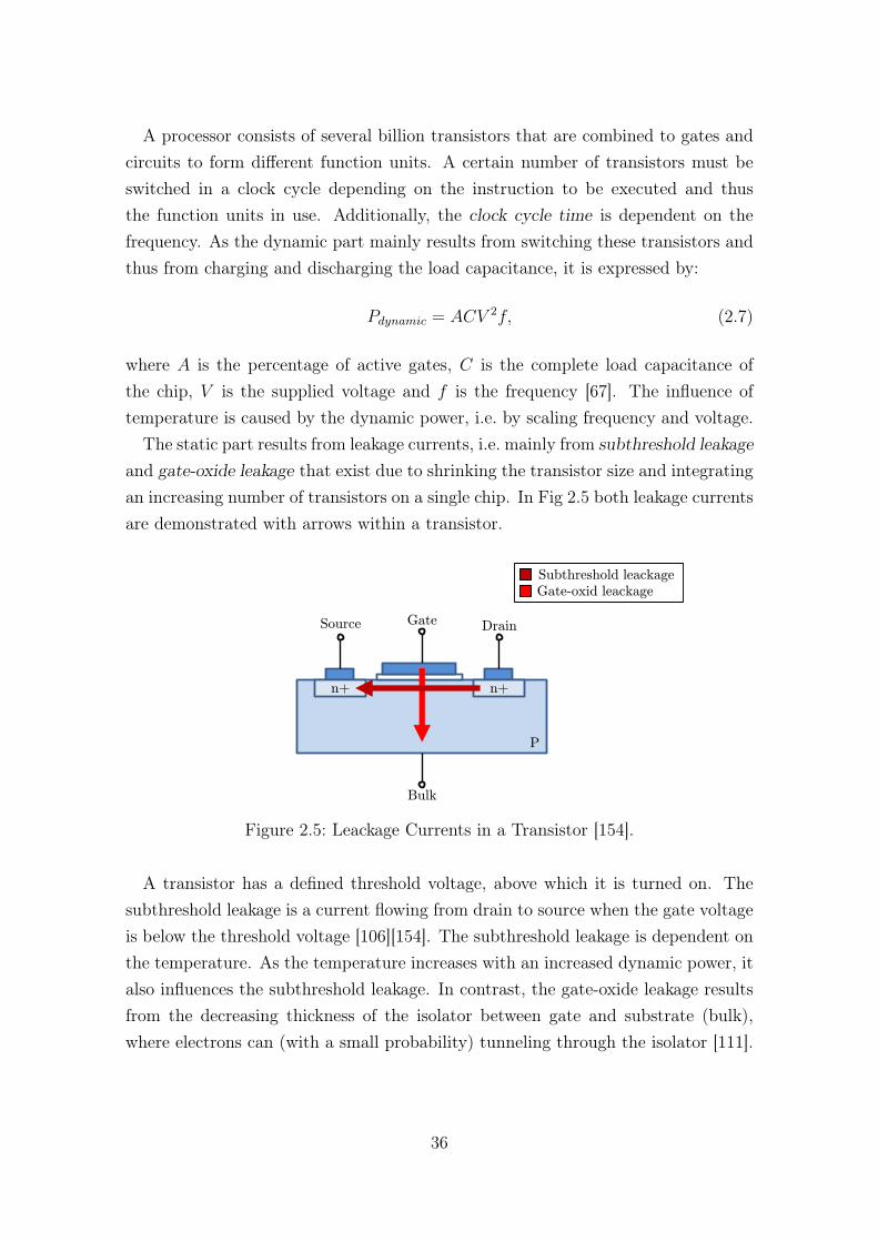
A processor consists of several billion transistors that are combined to gates andcircuits to form different function units. A certain number of transistors must beswitched in a clock cycle depending on the instruction to be executed and thusthe function units in use. Additionally, the clock cycle time is dependent on thefrequency. As the dynamic part mainly results from switching these transistors andthus from charging and discharging the load capacitance, it is expressed by:

Pdynamic = ACV 2f, (2.7)

where A is the percentage of active gates, C is the complete load capacitance ofthe chip, V is the supplied voltage and f is the frequency [67]. The influence oftemperature is caused by the dynamic power, i.e. by scaling frequency and voltage.

The static part results from leakage currents, i.e. mainly from subthreshold leakageand gate-oxide leakage that exist due to shrinking the transistor size and integratingan increasing number of transistors on a single chip. In Fig 2.5 both leakage currentsare demonstrated with arrows within a transistor.

Source Drain Gate

Bulk

n+ n+

P

Subthreshold leackage

Gate-oxid leackage

Figure 2.5: Leackage Currents in a Transistor [154].

A transistor has a defined threshold voltage, above which it is turned on. Thesubthreshold leakage is a current flowing from drain to source when the gate voltageis below the threshold voltage [106][154]. The subthreshold leakage is dependent onthe temperature. As the temperature increases with an increased dynamic power, italso influences the subthreshold leakage. In contrast, the gate-oxide leakage resultsfrom the decreasing thickness of the isolator between gate and substrate (bulk),where electrons can (with a small probability) tunneling through the isolator [111].

36

2.5.2 Modeling

To predict the energy consumption for a task and finally for an entire schedule, anappropriate power model of the processor (core) is mandatory or at least a tablewith real frequency/power consumption pairs. Basically, a model is a simplifiedrepresentation of the reality. The complexity of a model increases significantly withits accuracy. As the power consumption of a processor depends on several factors,like the temperature, instruction mix, usage rate and technology of the processor,there exist numerous approaches in the literature to model the power consumptionof a processor with varying complexities and accuracies, like in [23], [45], [71] or[170]. In general, without considering a specific processor, typically a quadraticor cubic frequency function is assumed, as the frequency and voltage are looselylinearly correlated5. Therefore, the power consumption for a given frequency f isexpressed by:

P (f) = c+ fα : 2 ≤ α ≤ 3, (2.8)

where c is a constant for the static power consumption and fα is for the dynamicpower consumption [7]. For a certain task workload wi, the runtime ri of a task ata given frequency fi results in:

ri =wifi. (2.9)

The energy consumption for an entire schedule (without considering the energyconsumption for idle times) is the sum of the energy consumptions for all tasks andis expressed by:

E =∑i

Ei =∑i

ri · P (fi). (2.10)

In such a generalized model, usually a continuous frequency scaling is assumed.While a processor typically supports only several discrete frequencies, each mod-eled frequency f can be "simulated" by a linear interpolation as demonstrated byEitschberger and Keller [55]. A task i then runs for a fraction β of the runtime riwith a higher supported frequency fhigh and for the remaining time 1 − β with alower supported frequency flow, so that f = β · fhigh + (1 − β) · flow. In Fig. 2.6,an example is demonstrated, where a task runs for five time units at a modeled fre-quency of 1.8 GHz (GigaHertz) and the corresponding distribution of the runtimewith discrete frequencies 1 GHz and 2 GHz.

5For a given voltage there is a maximum frequency and for a desired frequency there is a minimumvoltage required.

37

Time (t) 1 2 3 4 5

1.8 GHz

2 GHz 1 GHz

0

Figure 2.6: Task Runtime with a Modeled Continuous Frequency (Top) and withDiscrete Frequencies (Bottom).

The energy consumption for a task i with runtime ri at a simulated frequency fican then be expressed by:

E(fi, ri) = E(flow, β · ri) + E(fhigh, (1− β) · ri). (2.11)

The difference in energy consumption for continuous and discrete frequency scal-ing is very small, so that it often is neglected. In Fig. 2.7, the energy curves forcontinuous (modeled) and discrete (simulated) frequencies for one second are shown.

Simulated frequency Modeled frequency

Ener

gy (

J)

Frequency (GHz)

0.4 0.6 0.8 1 1.2 1.4 1.6 1.8 2

8

7

6

5

4

3

2

1

0

Figure 2.7: Energy Consumption for Continuous and Discrete Frequencies.

In this example a frequency range between 0.5 and 2 GHz is used with discretefrequencies of 0.5, 0.8, 1.1, 1.4, 1.7 and 2.0 GHz. As power model P (f) = f 3 isassumed. Between each discrete frequency pair ((fi, E(fi), (fi+1, E(fi+1)), the energyfor simulated frequencies results in a straight line, that connects both frequency

38

points. Idle times are often neglected, as modern processors typically supports sleepstates with a very low power consumption (compared to the power consumption ofa task).

2.5.3 Energy-efficient Scheduling

The information about the power consumption of a processor (core) at a certain fre-quency, either given by a power model or by a table of frequencies with correspondingreal power values, can be included into the scheduling process to optimize the energyconsumption for a task and finally for an entire schedule. Basically DVFS and DPMare used to construct an energy-efficient schedule. While DVFS is used to scale thefrequency and voltage of a processor during runtime, DPM is usually consideredfor longer idle times to switch a processor into a sleep state. To further reduce theenergy consumption, combinations of both techniques are used in scheduling. Nextto the use of these techniques also approaches exist that reduce the energy con-sumption by shutting down processors completely and scheduling the tasks onto theremaining processors. As there exist a huge number of energy-efficient approachesin the literature, only exemplary representatives are presented in the following:

Approaches using DPM Lu et al. [121] present an online low-power task schedul-ing approach for multiple devices that uses DPM. They focus on clustering idleperiods to increase the time for shutdowns and to reduce state-transition delays.They consider the difference in energy for idle periods, when switching to a sleepstate mode or when staying in an active mode.

In [122], Ma et al. present an energy-efficient scheduling algorithm for tasks ontoa cluster system without DVFS functionality. They propose a combination of taskclustering and task duplication to reduce the time and energy for communicationand DPM to decrease the static power of processing elements in idle phases. Thepower consumption is calculated by using technical parameters of the test system.

Baptiste [20] presents a polynomial time algorithm. He focuses on scheduling unittasks, i.e. the processing time for all tasks remains one time unit, and on minimizingthe number of idle periods. He assumes for each task a release date and a deadline.

Rizvandi and Zomaya [153] present a survey of DPM and DVFS scheduling algo-rithms for cloud systems as well as Jha [97] for uniprocessor and distributed systems.

39

Approaches using DVFS In [157], Ruan et al. present an energy-efficient schedul-ing approach called TDVAS6 for parallel applications on clusters. They assumeprecedence constraints between the tasks and use DVFS to reduce the voltage andfrequency for tasks followed by a gap or directly during idle periods without increas-ing the makespan. As power model P = C · V 2 · f is assumed. The voltage andfrequency levels are given by the system parameters of the used test system.

Lee [112] presents another scheduling approach for multicore processors. He con-siders multiple periodic real-time tasks and assumes situations with more cores thanrunning tasks. In the proposed scheduling heuristic, tasks are parallelized onto sev-eral cores, frequencies are scaled down if possible and unused cores are shut down tominimize the energy consumption. A table of power, frequency and voltage valuesis given for a test system and the energy consumption per cycle is calculated by thepower consumption divided by the frequency.

Huang et al. [86] present an energy-efficient mixed-criticality scheduling approach.They consider DVFS to speedup critical tasks that do not meet their deadlines andto slow down tasks in situations, where tasks finish before the deadlines. They usea cubic power model and assume continuous frequencies.

In [185], Yang et al. present an approximation algorithm for energy-efficientscheduling on a MP-SoC. They assume homogeneous cores that can either be switch-ed off or have to operate at the same voltage level. They consider frame-based tasksthat are ready at time 0 and share a common deadline. Their approximation algo-rithm yield an approximation ratio of 2.371.

For malleable streaming tasks, Kessler et al. [104] present an approach calledcrown scheduling. They propose a static combined optimization of resource alloca-tion, mapping and DVFS to optimize energy efficiency under throughput constraintswith the help of an ILP. They consider dynamic (crown) rescaling when not all tasksare data ready. As power model, a cubic frequency function is used. As extension,Melot et al. [126] present several additional heuristics for crown scheduling.

Mishra et al. [129] present an energy aware scheduling approach for distributedreal-time systems. They consider both static and dynamic energy management.They assume tasks with precedence constraints and integrate DVFS in already ex-isting schedules to statically generate energy-efficient schedules. During execution,they further use DVFS dynamically in case of unexpected execution delays.

Further investigations on energy-efficient scheduling using DVFS can be founde.g. in [26], [119] or [189].

6A long form of TDVAS is not defined by the authors.

40

Approaches using DPM and DVFS In [41], Chen et al. present an energy op-timization for real-time MP-SoCs with DVFS and DPM. They assume tasks withprecedence constraints that share a common deadline. They consider both staticand dynamic power consumption and discrete voltage/frequency levels. A mixedILP is proposed to find energy optimized schedules when using DVFS and DPM.

He and Müller [80] present an online energy-efficient scheduling approach for com-ponent oriented systems. They consider hard real-time based tasks and propose asimulated annealing based optimization algorithm. In contrast to many other ap-proaches, they also consider multiple sleep states and switching overhead.

Rong and Pedram [155] present a power-aware scheduling approach for hardreal-time systems. They assume periodic tasks with precedence constraints. Theypresent an ILP-formulation and propose also a three-step heuristic to minimize theenergy consumption. In a first step the tasks are ordered, then the voltage is as-signed, and finally a refinement step follows.

In [18], Bambagini et al. present a survey of energy-aware scheduling approachesfor real-time systems. They differentiate between DPM, DFVS, and combined al-gorithms for uniprocessor and multiprocessor systems and propose a taxonomy ofenergy-aware scheduling algorithms.

Zhuravlev et al. [194] present a survey of energy-cognizant scheduling techniques.Next to DPM and DVFS algorithms, also thermal aware approaches and schedulingalgorithms for heterogeneous systems are considered.

Albers [7] presents energy-efficient algorithms. She considers DVFS and DPM andpresents algorithms for various scheduling goals like minimizing the temperature,response time, or fulfill deadline constraints. Additionally, she presents approachesfor wireless networks.

Other Approaches For example, Pinel et al. [140] present a two-phase heuristicfor mapping independent tasks onto a distributed system to minimize the makespan.They consider energy efficiency by proposing to add low power computing nodes tothe distributed system.

In [113], Lenhardt presents approaches to distribute the load in server farms tosave energy. Not only an efficient load level in terms of energy savings withoutsignificant performance losses is presented, but also fluctuations in the load areconsidered that can be balanced by switching off some servers or transferring themto a sleep state mode and re-distributing the load to the remaining servers.

41

Cong and Yuan [47] present an energy-efficient scheduling approach for heteroge-neous multicore systems. They map programs onto the most appropriate core basedon program phases and use a combination of static analysis and runtime scheduling.

2.5.4 From the Model to the Real World

In real computer systems, several limitations and issues exist in hard- and softwarethat reduce possibilities to utilize energy-efficient scheduling. Continuous frequencyscaling for example is impossible, as processors only support several discrete fre-quencies. The ACPI standard recommends up to 16 frequency levels [82]. Thevoltage range decreases with a reduced transistor size. Therefore, energy improve-ments resulting from using DVFS will be getting smaller in the future, as the voltageis the most significant factor that influences the power consumption. Additionally,by shrinking the transistor size and integrating further transistors into a single chip,the heat is getting higher, resulting from switching transistors. This leads to so-called dark silicon, i.e. not all parts of a processor can be used at the same time.Therefore, the trend is changing towards processors including different cores, e.g.low power and high performance cores that are switched off, when they are idle [57].

Depending on the timescale that is assumed for a schedule, also the switching timesbetween different frequencies and voltages are becoming important, like for stream-ing applications as demonstrated by Eitschberger and Keller [55]. Additionally,in some operating systems the accessibility to control DVFS options is restricted.Linux-based systems typically support different governors that can be set to changethe frequency scaling behavior or to make DVFS accessible to applications that arebuilt on top of the operating system. A corresponding API is the so-called CPUFreq(Central Processing Unit Frequency) [88]. In contrast, Windows-based systems donot allow any access to DVFS by other applications or by a user. Also the kind ofprocessor is important for energy-efficient scheduling. For example the voltage formost processors can only be scaled for all cores together within the processor, butnot separately, as the voltage regulator for the whole processor is typically placed onthe mainboard. One type of processors, where a separate voltage scaling per core ispossible, are the Haswell-based server processors from Intel [76]. In this architecturethe voltage regulators for each core are directly included on the processor chip.

Modern processors support a so-called turbo frequency that is significantly higherthan the other frequency levels. The turbo frequency is influenced by several factors,like the number of active cores or the temperature of the processor and therefore it

42

varies over time. It can only be used for a certain time span because of temperaturereasons. Otherwise, throttling effects can occur, i.e. switching between a lowerfrequency and a turbo frequency during execution to reduce the temperature of theprocessor [82].

2.5.5 Measuring Power Consumption

The classical way to measure the power consumption of a processor is to use anexternal multimeter. Next to this, several modern processors directly support mea-surement features that can be used to evaluate the power consumption. For examplethe RAPL (Running Average Power Limit) interface in Intels’ processors [91] thatwas introduced in the Sandy-bridge architecture. The RAPL interface is basicallyused to set and control power limitations of a processor with the help of performancecounters and MSRs (Model-Specific Registers). Some of these performance countersprovide information about the power and energy consumption of different processorcomponents by using a software power model. In Tab. 2.1 all components are listedthat are (partly) supported by modern Intel processors. The MSRs are updated

Table 2.1: RAPL Domains and Corresponding Processor Components.Domain ComponentPackage (PKG) Complete processor chipPowerPlane0 (PP0) All processor coresPowerPlane1 (PP1) Processor uncore, mainly the GPUDynamic RAM (DRAM) Memory controller

every millisecond and the accuracy of the power and energy information is high incomparison to real measurements, like presented in [76], [77] and [190].

To access the MSRs with the power and energy information within a program,the PAPI (Performance Application Programming Interface)7 can be used [178]. Asthe MSRs are only accessibly in the kernel level, the user must either have rootpermissions or the executable. In combination with MPI only the latter one ispossible, as MPI cannot be used as root-user.

7PAPI is a project of the University of Tennessee to design, standardize, and implement an APIto access hardware performance counters.

43

44

3 Trade-off between Performance,Fault Tolerance and EnergyConsumption

In general, a trade-off describes a balancing of factors that are unattainable simul-taneously. Improving one of these leads to a worsening of the others. The behavioris similar related to a combination of the three optimization criteria: performance,fault tolerance, and energy consumption. A trade-off already exists if two of thesethree are considered. While there are several approaches in the literature for thesetwo-dimensional optimizations, a combination of all three criteria, especially for du-plication based task graph scheduling, has not been considered yet. Sect. 3.1 firstlydescribes the trade-offs for all two-dimensional combinations. Then, for each combi-nation exemplary related existing approaches are presented. In Sect. 3.2 the indirecttrade-off between the fault-free case and the fault case is described. In Sect. 3.3 thethree-dimensional optimization problem is explained. Finally, in Sect. 3.4 upper andlower bounds for the three criteria are given.

3.1 Two-dimensional Optimization

A common practice for two-dimensional optimizations with a trade-off between theoptimization criteria is to fix one criterion, while the other is optimized. For schedul-ing in general this means that either a fixed deadline (or makespan) or a fixed energybudget is assumed.

3.1.1 Performance vs. Fault Tolerance

Scheduling goals either focus on minimizing the makespan and thus maximizingthe performance of a schedule, or on minimizing the energy consumption for theexecution of a schedule (see Sect. 2.3). Here, the first approach is assumed. In

45

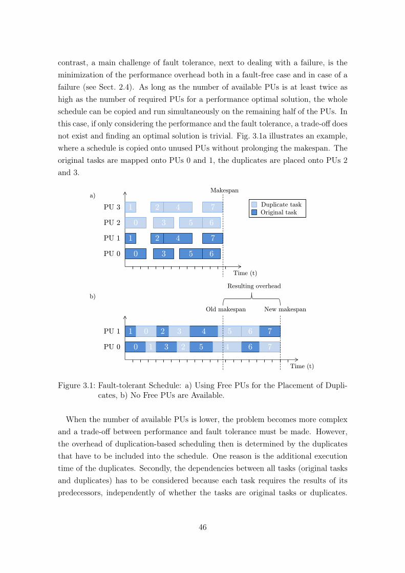
contrast, a main challenge of fault tolerance, next to dealing with a failure, is theminimization of the performance overhead both in a fault-free case and in case of afailure (see Sect. 2.4). As long as the number of available PUs is at least twice ashigh as the number of required PUs for a performance optimal solution, the wholeschedule can be copied and run simultaneously on the remaining half of the PUs. Inthis case, if only considering the performance and the fault tolerance, a trade-off doesnot exist and finding an optimal solution is trivial. Fig. 3.1a illustrates an example,where a schedule is copied onto unused PUs without prolonging the makespan. Theoriginal tasks are mapped onto PUs 0 and 1, the duplicates are placed onto PUs 2and 3.

PU 0

PU 1

0 3 5 6

2 4 7 1 0 3 5 6

2 4 7 1

Time (t)

Old makespan New makespan

Resulting overhead

PU 0

PU 1

PU 2

PU 3

0 3 5 6

2 4 7 1

0 3 5 6

2 4 7 1 Duplicate task

Original task

Time (t)

Makespan a)

b)

Figure 3.1: Fault-tolerant Schedule: a) Using Free PUs for the Placement of Dupli-cates, b) No Free PUs are Available.

When the number of available PUs is lower, the problem becomes more complexand a trade-off between performance and fault tolerance must be made. However,the overhead of duplication-based scheduling then is determined by the duplicatesthat have to be included into the schedule. One reason is the additional executiontime of the duplicates. Secondly, the dependencies between all tasks (original tasksand duplicates) has to be considered because each task requires the results of itspredecessors, independently of whether the tasks are original tasks or duplicates.

46

Fig. 3.1b illustrates the fault-tolerant schedule when free PUs are unavailable. Now,the makespan is increased by placing the duplicates directly between the originaltasks resulting in a performance overhead. Usually, the focus lies on the fault-free case, because in most environments a failure occurs infrequently. Therefore,minimizing the performance overhead in this case is desired.

Fechner et al. [59] present a fault-tolerant duplication-based scheduling approachfor grids that guarantees no overhead in a fault-free case. They assume to have analready existing schedule (and task graph) and extend this schedule by includinga duplicate for each original task. They focus on homogeneous PUs and assume afail-stop model. To reduce the performance overhead of the schedule, an originaltask sends a commit message to its corresponding duplicate after it has finished sothat the duplicate can be aborted.

Hashimoto et al. [79] present a fault-tolerant duplication-based scheduling algo-rithm for multiprocessor systems. They assume to have homogeneous processingelements and a fail-stop model. In their work, a single processor failure is consid-ered. The algorithm consists of two phases, one for the partitioning of the parallelprogram into subsets of tasks, the other for duplicating and scheduling the tasks inthe subset. The duplication is done in two steps: In the first step, the tasks areduplicated to minimize the communication delays and thus to increase the perfor-mance. To reach the fault tolerance, a second step is used to duplicate tasks thatare not duplicated in the first step.

In [83], Hongxia and Xin present a fault-tolerant scheduling algorithm with dy-namic replication, called DRFT-algorithm (Dynamic Replication of Fault-Tolerantscheduling). They combine an active and passive mode of backup tasks to reduce theperformance overhead in case of a failure. For each task a backup level is calculatedto decide how long the active and passive backups should be.

Jayadivya et al. [95] present a fault-tolerant workflow scheduling approach forCloud Computing, called FTWS (Fault-Tolerant Workflow Scheduling). They as-sume to have a predefined deadline, within which the schedule must be completed.To get a good performance while tolerating failures, a combination of replicationand resubmission of tasks is used. Therefore, a heuristic metric is calculated to findthe trade-off between replication and resubmission.

Izosimov et al. [93] present an algorithm that handles the transparency/perfor-mance trade-offs of fault-tolerant embedded systems. They focus on transient faultsin safety-critical systems. The transparency requirements are handled at the ap-plication level and give the designer the opportunity to trade-off between memory

47

requirements and debuggability and performance. It reduces the overhead due tofault tolerance.

In [10], Anglano and Canonico extend a knowledge-free scheduler called WQR(WorkQueue with Replication) scheduler that does not base its decisions on thestatus of resources or characteristics of applications. They focus on bag-of-tasksgrid applications and try to maximize the performance by using task replication.They consider heterogeneous systems and let the replicated tasks run on processingunits, whenever they are in idle mode. In order to achieve fault-tolerance and goodapplication performance, they use automatic restarting of tasks and checkpointingin their fault-tolerant extension of WQR, so-called WQR-FT (Fault-Tolerant).

Further investigations on performance and fault-tolerance in scheduling can befound e.g. in [3], [24] and [169].

3.1.2 Performance vs. Energy Consumption

The performance of a schedule is dependent on the mapping of the tasks. Themore an application can be parallelized the better is the performance. Addition-ally modern processors support several frequencies at which a processor can run.Thus, the tasks should be accelerated as much as possible, i.e. use the highest sup-ported frequency of a processor to achieve the highest performance. As described inSect. 2.5, the dynamic power consumption of a processor (core) is usually modeledby a quadratic or cubic frequency function. From the perspective of energy consump-tion a low frequency typically leads to better results than a high frequency. However,this is highly dependent on the processor type, because in real systems there areseveral other factors that influence the power consumption of a processor and thusthe energy consumption of a schedule (e.g. the static power or the idle power etc.)In Fig. 3.2 an example schedule is given (a) and the resulting performance overheadis shown when the frequency is scaled down to save energy (b).

Pruhs et al. present in [147] an approximation-algorithm to optimize the perfor-mance of a schedule by scaling the processor frequencies, when a certain energybudget is given. They consider continuous frequencies and tasks with precedenceconstraints. As power model a cubic function f 3 is used. They show that withthese assumptions the aggregate powers of the processors are constant, i.e. the sumof the processors’ power consumptions is constant over time in any locally optimalschedule. However, to find an optimized solution the problem can be restricted toschedules with those properties (so called constant power schedules).

48

PU 0

PU 1

0 3 5 6

2 4 7 1

Original task

Time (t)

Makespan a)

New makespan

PU 0

PU 1

0 3 5 6

2 4 7 1

Time (t)

Old makespan b)

Resulting overhead

Figure 3.2: Example Schedule: a) Running at a High Frequency (e.g. 2 GHz), b)Reducing Energy Consumption by Scaling Down the Frequencies (e.g.to 1 GHz).

In [105], Kianzad et al. present a framework, called CASPER (Combined As-signment, Scheduling, and PowER management), that uses a genetic algorithm tofind an optimized schedule. They consider both homogeneous and heterogeneoussystems and use frequency scaling. The focus in their presented work lies on theintegration of the scheduling and scaling steps.

Singh and Auluck [162] present an integrated DVFS and duplication-based ap-proach for optimizing power and performance in heterogeneous multiprocessors.They use a combination of DVFS i.e. let the tasks run on low voltages and fre-quencies and duplicating tasks on multiple processors to reduce the communicationdelay between the tasks. A Mixed Integer Programming (MIP) formulation is givento get a better power consumption and performance at the same time. They showthat their approach leads to significant improvements for both the processor powerand the total power, i.e. the processor power and the communication.

Ma et al. [123] present an algorithm, called EOTD (Energy Optimization schedul-ing for Task Dependent graph) that uses task clustering to reduce both communica-tion time and energy consumption. DVS is considered to decrease dynamic power ofprocessing elements without violating a user predefined deadline. Also static poweris reduced by dynamic power management and binary search techniques.

49

In [180], Wang et al. discuss the relationship between energy consumption andperformance in clusters with DVFS. They propose scheduling heuristics to minimizethe energy consumption of a schedule without prolonging the makespan. Theyreduce the energy consumption by using the slack time for non-critical tasks, toslowdown the tasks by scaling down the frequencies. Additionally, they considerenergy-performance trade-off scheduling by increasing the makespan of a schedulewithin an affordable limit to reduce the energy consumption.

Li [115] presents a performance analysis of power-aware task scheduling algo-rithms and shows that on a multiprocessor computer, the problem of minimizingthe schedule length with energy constraint and the vice versa problem, minimizingenergy consumption with schedule length constraint are equivalent to the sum ofpowers problem. He analyses the performance of list scheduling and equal-speedalgorithms by comparing the performance of the algorithms with optimal solutionsanalytically.

Aupy et al. [12] present a survey of different energy-efficient approaches. Theydescribe models for data centers and energy models next to a case study about taskgraph scheduling and replica placements.

Further investigations on performance and energy consumption in scheduling canbe found e.g. in [99], [128] and [159].

3.1.3 Fault Tolerance vs. Energy Consumption

In any case where fault tolerance is warranted, some kind of redundancy is necessary(see Sect. 2.4). In duplication-based scheduling the redundancy is used in the formof task copies, so-called Ds (Duplicates). A D can only be started, when it hasreceived all results from its predecessors and when no other task is running on thecorresponding PU. We assume that a D can be aborted when the correspondingoriginal task has finished correctly. To save energy, a D can also be placed withruntime (and thus energy) zero at the end of the corresponding original task, becauseit never has to be started in the fault-free case, i.e. when the completion of theoriginal task is successful. Such a D with runtime zero is then called DD (DummyDuplicate). To get a better fault tolerance (in terms of performance overhead in caseof a failure) the duplicates should be executed simultaneously to the original tasksor at least as long as possible. However, increasing the execution time of duplicatesleads to an increased energy consumption. Fig. 3.3 shows this behavior with anexample schedule.

50

PU 0

PU 1

0 3 5 6

2 4 7 1 0 5

7

Duplicate task

Original task

Time (t)

Makespan

DD1 DD2 DD4

DD3 DD6 a)

PU 0

PU 1

0 3 5 6

2 4 7 1

Time (t)

Makespan

DD1 DD2 DD4

DD3 DD6 b) DD0 DD5

DD7

Figure 3.3: Fault-tolerant Schedule: a) Using Dummies and Duplicates to Increasethe Fault Tolerance, b) Only Using Dummies to Get a Better EnergyConsumption.

In the upper case, duplicates are executed as long as possible without prolongingthe makespan. In the bottom case, only DDs are used. Hence, in the fault-free caseno energy has to be consumed for the DDs.

In terms of energy consumption the tasks should run with a low frequency tosave energy. But slowing down the tasks without changing the mapping of the tasksresults in different gaps and thus to another placement of the duplicates that mightresult in a higher performance overhead in case of a failure. Additionally, also theduplicates have to be slowed down because otherwise a duplicate would finish earlierthan the corresponding original task. Thus, the duplicates are prolonged and gapsmight become too small for the placement of whole duplicates. In this case, eitherthe succeeding tasks have to be shifted and the makespan is significantly increasedor the duplicates can only be executed for a short time before the next original task

51

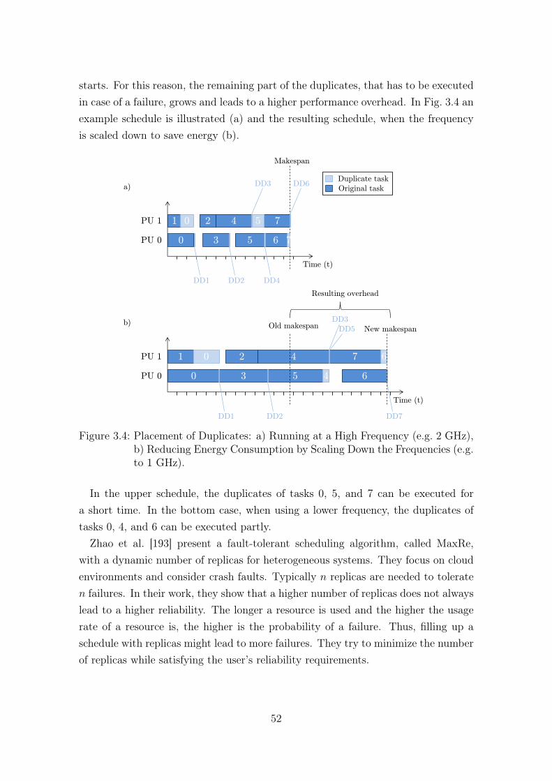
starts. For this reason, the remaining part of the duplicates, that has to be executedin case of a failure, grows and leads to a higher performance overhead. In Fig. 3.4 anexample schedule is illustrated (a) and the resulting schedule, when the frequencyis scaled down to save energy (b).

PU 0

PU 1

0 3 5 6

2 4 7 1 0 5

7

Duplicate task

Original task

Time (t)

Makespan

DD1 DD2 DD4

DD3 DD6 a)

New makespan

PU 0

PU 1

0 3 5 6

2 4 7 1

Time (t)

Old makespan b)

Resulting overhead

0

DD3

DD5

4

6

DD7 DD1 DD2

Figure 3.4: Placement of Duplicates: a) Running at a High Frequency (e.g. 2 GHz),b) Reducing Energy Consumption by Scaling Down the Frequencies (e.g.to 1 GHz).

In the upper schedule, the duplicates of tasks 0, 5, and 7 can be executed fora short time. In the bottom case, when using a lower frequency, the duplicates oftasks 0, 4, and 6 can be executed partly.

Zhao et al. [193] present a fault-tolerant scheduling algorithm, called MaxRe,with a dynamic number of replicas for heterogeneous systems. They focus on cloudenvironments and consider crash faults. Typically n replicas are needed to toleraten failures. In their work, they show that a higher number of replicas does not alwayslead to a higher reliability. The longer a resource is used and the higher the usagerate of a resource is, the higher is the probability of a failure. Thus, filling up aschedule with replicas might lead to more failures. They try to minimize the numberof replicas while satisfying the user’s reliability requirements.

52

Aupy et al. [12] also present some works about fault tolerance and energy efficiency,but with checkpointing instead of task duplication.

3.2 Fault-free Case vs. Fault Case

Yet another trade-off exists between the fault-free case and the fault case. Most im-provements in the fault-free case lead to some worsening in the fault case and viceversa. For example focusing on the performance in the fault-free case (not consider-ing the marginal case in Sect. 3.1.1) means using placeholders (so called Dummies)as duplicates where necessary and consider the communication times between allduplicates and original tasks only in case of a failure. Thus, the worsening of theperformance is shifted from the fault-free case into the fault case. When focusing onthe energy consumption in the fault-free case, the tasks (and thus the duplicates)are prolonged because the frequencies of the PUs are scaled down. In case of afailure, these duplicates cause a higher performance overhead, because they still runwith a low frequency. Focusing on the fault tolerance in the fault-free case improveson the one hand the performance overhead in case of a failure, but on the otherhand increases the energy consumption in the fault-free case. However, either thistrade-off must be considered directly when focusing on the fault-free case, or therehave to be other options and strategies for the fault-free case and in case of a fail-ure, so that the preferences of a user can be set independently in both cases. As theapproaches in the literature focus only on one of both cases, there does not existany work about a combined approach that considers directly this trade-off.

3.3 Three-dimensional Optimization: Performance

vs. Fault Tolerance vs. Energy Consumption

As seen in Sect. 3.1, a trade-off already exists in all two-dimensional cases. A com-bination of all three criteria, performance, fault tolerance and energy consumptionleads to several additional optimization parameters. While one criterion is improved,either one or both of the others are worsened. But it is unclear how this worsen-ing should be distributed to the other criteria. The main focus varies in differentsituations. For example, in a time critical environment, the performance is themost important criterion next to the fault tolerance. Thus, in this situation theperformance and the fault tolerance is usually favored over minimizing the energy

53

consumption. Another situation is that a failure occurs extremely rarely and thusthe energy consumption in a fault-free case becomes more important. Another ex-ample exists in mobile devices, such as smartphones and laptops, where the energyconsumption is the most important criterion next to the performance. Thus, themain focus is put on the energy consumption and on the performance while faulttolerance is neglected.

Especially for real-time systems, approaches are given in the literature, that com-bine all three criteria. The real-time constraint itself can be interpreted as theperformance criterion, because in such systems the execution of a task or schedulehas to be finished before a deadline. Thus, the performance is fixed while the othercriteria are improved. In real-time systems, the focus typically lies on transientfaults, where checkpointing or backup mechanisms are used to circumvent a fault.

For example, Cai et al. [37] present a greedy heuristic to reduce the energy con-sumption in fault-tolerant distributed embedded systems with time-constraints. Thefault tolerance is given by a combination of re-executing tasks and using replication.They assume a heterogeneous system environment where the processors are con-nected via a bus. They focus on transient faults and they use a reserved slackfor the re-execution. Their greedy heuristic searches for the task that consumesthe most energy and try to either change the mapping of the task or to include (ordelete) a replica. This procedure is repeated until all tasks are considered or until nofurther energy improvement can be achieved. Thus, in their work the makespan of aschedule and the fault tolerance is fixed while the energy consumption is improved.

In [6], Alam and Kumar present another approach. They assume that only onespecific transient fault could occur during the execution of a task. Checkpointing isused to tolerate faults and a fault is detected within the next checkpointing interval.Then, the last checkpoint is used to execute the remaining part of the task. Theminimization of the energy consumption is done by DVS, i.e. using a discrete voltagelevel with its corresponding clock speed. To achieve a good fault tolerance, they findthe optimal number of checkpoints to be included into the tasks. In their work, theperformance is fixed, while the fault tolerance and energy consumption is beingoptimized.

Tosun et al. [175] present a framework that is used to map a given real-timeembedded application under different optimization criteria onto a heterogeneouschip multiprocessor architecture. They consider energy consumption, performance,and fallibility (the opposite of reliability) as objective functions or constraints fortheir ILP formulation. Duplicating tasks is used to detect faults and DVS for energy

54

savings. The processors are connected via a shared bus system and communicationoverheads are neglected. A result checker after each task and its correspondingduplicate is used to find a fault. They focus on the trade-off between increasing thenumber of duplicates, energy consumption, and performance.

However, the alignment of the optimization is very situational and ultimatelydepends highly on the user preferences.

3.4 Estimation of Upper/Lower Bounds

3.4.1 Performance

Focusing on performance PE, the best solution is to parallelize an application asmuch as possible. Furthermore, the highest available frequency fhighest should beselected, if the system in use supports different frequencies. Then, a simple generalupper bound for the performance can be described as the following equation, wheremseq is the makespan in cycles, when all tasks are running in sequence and pmax ∈PU is the maximum number of PUs used:

PEbest =mseq

pmax · fhighest(3.1)

A lower bound for the performance can be achieved by running all tasks in se-quence on one PU with the lowest possible frequency flowest. Equation 3.2 showsthis context:

PEworst =mseq

1 · flowest(3.2)

3.4.2 Fault Tolerance

While a schedule is either fault-tolerant or not, in this thesis, the fault tolerance FTis rated by the performance overhead in case of a failure. Therefore, when focusingon the fault tolerance the best solution is to copy the whole schedule and execute itsimultaneously (completely independent) to the original one on other PUs. Then,both the performance, i.e. the makespan mft in case of a failure and in a fault-freecase m are equal. Accordingly, the performance overhead results to zero percent.

FTbest =mft −m

m· 100 = 0% (3.3)

55

However, the worst solution is when the schedule is not fault-tolerant and a failureoccurs directly before the end of the schedule execution. Then, the whole schedulehas to be repeated on p− 1 PUs and the makespan mft = 2 ·m in case of a failureis at least doubled in comparison to the fault-free case m. Thus, the performanceoverhead in case of a failure results in 100 percent.

FTworst ≥mft −m

m· 100 =

2 ·m−mm

· 100 = 100% (3.4)

3.4.3 Energy Consumption

The energy consumption for a schedule execution is highly dependent on the powerconsumption of the processors in use. As the power consumption of different pro-cessors varies significantly, a general upper or lower bound cannot be determined.Only when a specific processor or power model is considered, the boundaries canbe defined. However, instead of finding general boundaries, some factors are giventhat influence the energy consumption and thus the upper and lower bounds. Then,exemplary the lower and upper bounds for a simple cubic power model are described.

The power consumption of a processor (core) can be subdivided into a staticpart that is frequency independent and a dynamic part that depends on both thefrequency and the supplied voltage (see Sect. 2.5.2). When the static power con-sumption is high in comparison to the dynamic power consumption, using a certainfrequency influences the total power consumption a little. Thus, speeding up a taskby running at a high frequency is more energy-efficient than running at a low fre-quency. In contrast, when the static power consumption is low, it is better to scaledown the frequency and thus slowing down a task to get a low energy consumption.

The idle power consumption influences the lower and upper bounds significantly.When the idle power is high, a reduction of the idle times within a schedule wouldlead to better results than having a lot of gaps between the tasks. Thus, trying to fillup the gaps within a schedule with duplicates and shutting off all unused processorswould be better than using a free processor for the duplicates. If the idle power canbe neglected, because it is very low or cores can go to sleep mode, both solutionswould lead to the same energy behavior.

Another reason results from different instructions. For example, a task with manyload and store instructions leads to a different energy consumption than a task withmany arithmetic calculations and only a few load and store instructions.

56

It is important whether only the power consumption of a processor core is con-sidered or the power consumption of the whole processor. If the focus lies on theprocessor core, the static power consumption is very low, because there are only afew components within the core that influence the power consumption. From theperspective of a processor in total, there are many components like the memorycontroller, the low-level caches, graphic units etc. that also influence the power con-sumption. Additionally, some components might only be switched on when at leastone processor core is under load. So that the relation between running in idle modeand executing something on one core might be more complex than focusing only ona processor core and its components.

Starting from a simple cubic power model for the dynamic power consumption,i.e. at frequency f , a core consumes power proportional to f 3. The energy consump-tion of a task ti is then the product of power and task runtime which is inverselyproportional to the frequency. For simplicity, constant factors and low-order termsare left out. Then an upper and lower bound for the energy consumption can begiven by:

Ebest =n−1∑i=0

tiflowest

· f 3lowest, (3.5)

Eworst =n−1∑i=0

tifhighest

· f 3highest. (3.6)

In this model, the idle power and power for communication is neglected and thusonly the sum of all tasks has to be considered but not the concrete mapping orscheduling or the resulting makespan.

57

58

4 Fault-tolerant andEnergy-efficient Scheduling

In this chapter, various approaches that include fault-tolerant and energy-efficientaspects into the scheduling process are presented. Starting with the assumptionsin Sect. 4.1, fault-tolerant scheduling heuristics are given in Sect. 4.2. Next tothe previous work, new fault-tolerant heuristics are introduced. In Sect. 4.3 severalextensions, i.e. heuristics and options are presented that combine energy savings andinvestments with the fault-tolerant approaches for both the fault-free case and incase of a failure. As these extensions affect different parts of the heuristics, possiblecombinations of those are discussed in Sect. 4.4 and new combined strategies areproposed that reflect different preferences of a user. Finally, energy-optimal solutionsare presented in Sect. 4.5.

4.1 Assumptions

In this work, homogeneous systems with a fully meshed network are considered.Starting from an already existing schedule (and task graph), the following schedul-ing algorithms are used afterwards to include fault tolerance and energy efficiencyaspects. Thus, these algorithms are not restricted to specific schedulers and there-fore can be combined with every static scheduling method. To be independent froma concrete system, one assumption and also goal is to support the scheduling andexecution without any changes of the operating system. Hence, a correspondingscheduler and runtime system is built on top of the operating system.

As failure model, the crash model is assumed (see Sect. 2.4) and a single perma-nent fault can occur during the runtime of a schedule. For simplification, possiblebottlenecks e.g. in memory or network bandwidth are not considered. The proba-bility of a fault is neglected in the following presentation.

A maximum load level of a PU is considered by assuming computational taskswith a standard instruction mix. Influences in the power consumption due to the

59

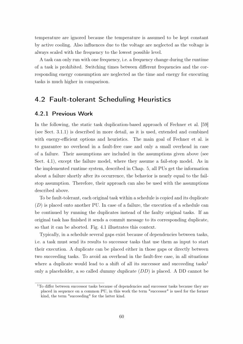
temperature are ignored because the temperature is assumed to be kept constantby active cooling. Also influences due to the voltage are neglected as the voltage isalways scaled with the frequency to the lowest possible level.

A task can only run with one frequency, i.e. a frequency change during the runtimeof a task is prohibited. Switching times between different frequencies and the cor-responding energy consumption are neglected as the time and energy for executingtasks is much higher in comparison.

4.2 Fault-tolerant Scheduling Heuristics

4.2.1 Previous Work

In the following, the static task duplication-based approach of Fechner et al. [59](see Sect. 3.1.1) is described in more detail, as it is used, extended and combinedwith energy-efficient options and heuristics. The main goal of Fechner et al. isto guarantee no overhead in a fault-free case and only a small overhead in caseof a failure. Their assumptions are included in the assumptions given above (seeSect. 4.1), except the failure model, where they assume a fail-stop model. As inthe implemented runtime system, described in Chap. 5, all PUs get the informationabout a failure shortly after its occurrence, the behavior is nearly equal to the fail-stop assumption. Therefore, their approach can also be used with the assumptionsdescribed above.

To be fault-tolerant, each original task within a schedule is copied and its duplicate(D) is placed onto another PU. In case of a failure, the execution of a schedule canbe continued by running the duplicates instead of the faulty original tasks. If anoriginal task has finished it sends a commit message to its corresponding duplicate,so that it can be aborted. Fig. 4.1 illustrates this context.

Typically, in a schedule several gaps exist because of dependencies between tasks,i.e. a task must send its results to successor tasks that use them as input to starttheir execution. A duplicate can be placed either in those gaps or directly betweentwo succeeding tasks. To avoid an overhead in the fault-free case, in all situationswhere a duplicate would lead to a shift of all its successor and succeeding tasks1

only a placeholder, a so called dummy duplicate (DD) is placed. A DD cannot be

1To differ between successor tasks because of dependencies and successor tasks because they areplaced in sequence on a common PU, in this work the term "successor" is used for the formerkind, the term "succeeding" for the latter kind.

60

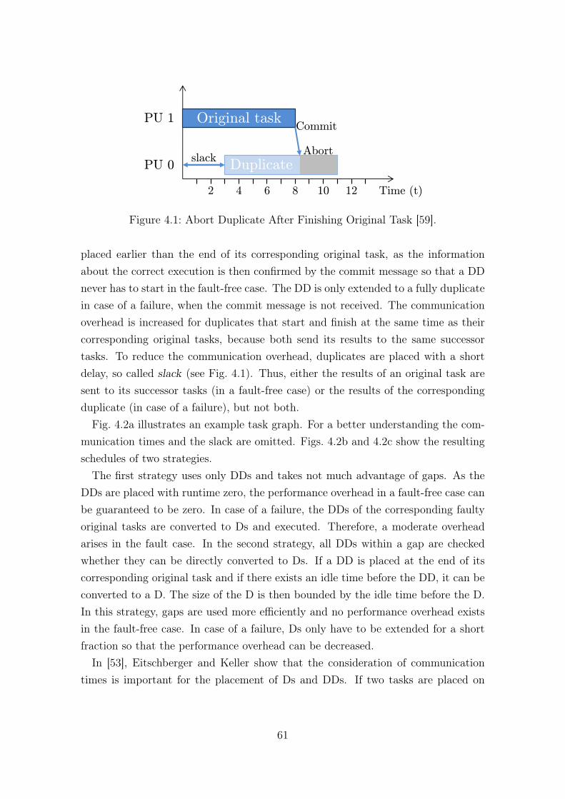
PU 0

PU 1

Time (t) 2 4 6 8 10 12

Original task

α

0 1

2

3

4

Ω

a)

b)

Commit

Abort slack

Duplicate

Figure 4.1: Abort Duplicate After Finishing Original Task [59].

placed earlier than the end of its corresponding original task, as the informationabout the correct execution is then confirmed by the commit message so that a DDnever has to start in the fault-free case. The DD is only extended to a fully duplicatein case of a failure, when the commit message is not received. The communicationoverhead is increased for duplicates that start and finish at the same time as theircorresponding original tasks, because both send its results to the same successortasks. To reduce the communication overhead, duplicates are placed with a shortdelay, so called slack (see Fig. 4.1). Thus, either the results of an original task aresent to its successor tasks (in a fault-free case) or the results of the correspondingduplicate (in case of a failure), but not both.

Fig. 4.2a illustrates an example task graph. For a better understanding the com-munication times and the slack are omitted. Figs. 4.2b and 4.2c show the resultingschedules of two strategies.

The first strategy uses only DDs and takes not much advantage of gaps. As theDDs are placed with runtime zero, the performance overhead in a fault-free case canbe guaranteed to be zero. In case of a failure, the DDs of the corresponding faultyoriginal tasks are converted to Ds and executed. Therefore, a moderate overheadarises in the fault case. In the second strategy, all DDs within a gap are checkedwhether they can be directly converted to Ds. If a DD is placed at the end of itscorresponding original task and if there exists an idle time before the DD, it can beconverted to a D. The size of the D is then bounded by the idle time before the D.In this strategy, gaps are used more efficiently and no performance overhead existsin the fault-free case. In case of a failure, Ds only have to be extended for a shortfraction so that the performance overhead can be decreased.

In [53], Eitschberger and Keller show that the consideration of communicationtimes is important for the placement of Ds and DDs. If two tasks are placed on

61

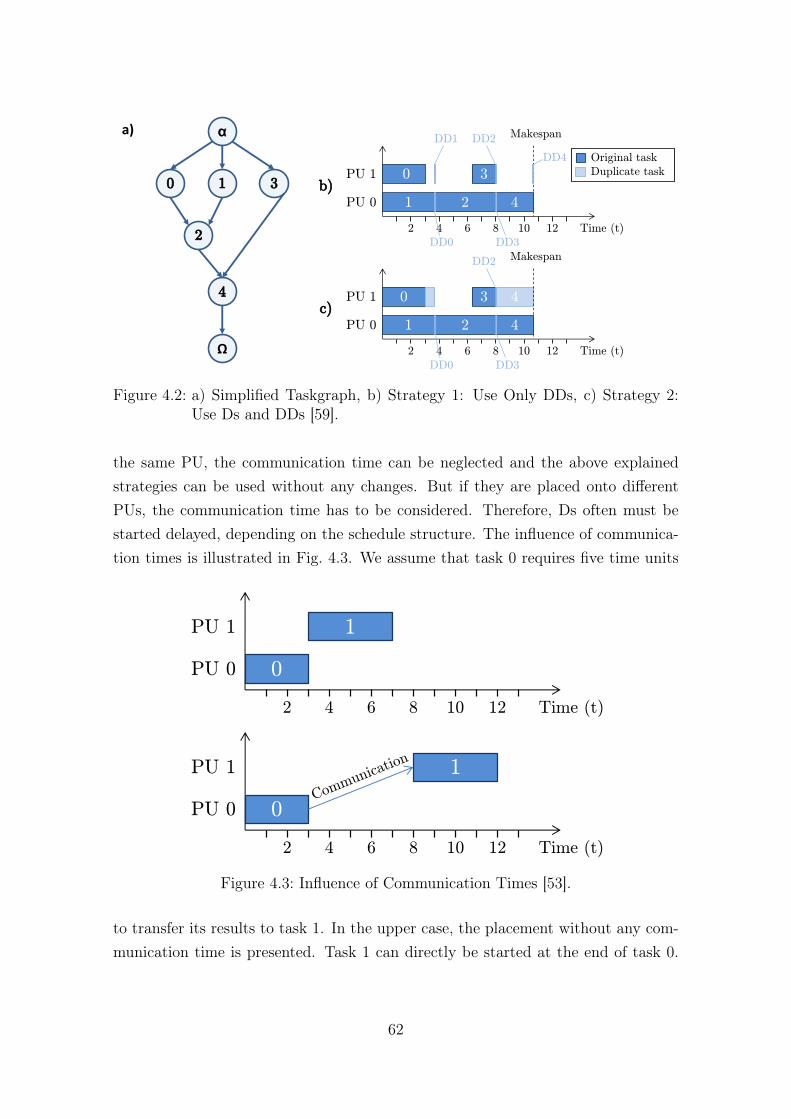
4

2 PU 0

PU 1 3

Original task

Duplicate task

Time (t)

Makespan

2 4 6 8 10 12

0

1 4

DD4

DD0

DD2

DD3

α

0 1

2

3

4

Ω

a)

b)

c) 2 PU 0

PU 1 3

Time (t)

Makespan

2 4 6 8 10 12

0

1 4

DD0

DD2

DD3

DD1

1

Figure 4.2: a) Simplified Taskgraph, b) Strategy 1: Use Only DDs, c) Strategy 2:Use Ds and DDs [59].

the same PU, the communication time can be neglected and the above explainedstrategies can be used without any changes. But if they are placed onto differentPUs, the communication time has to be considered. Therefore, Ds often must bestarted delayed, depending on the schedule structure. The influence of communica-tion times is illustrated in Fig. 4.3. We assume that task 0 requires five time units

PU 0

PU 1

Time (t) 2 4 6 8 10 12

0

1

PU 0

PU 1

2 4 6 8 10 12

0

1

Time (t)

Figure 4.3: Influence of Communication Times [53].

to transfer its results to task 1. In the upper case, the placement without any com-munication time is presented. Task 1 can directly be started at the end of task 0.

62

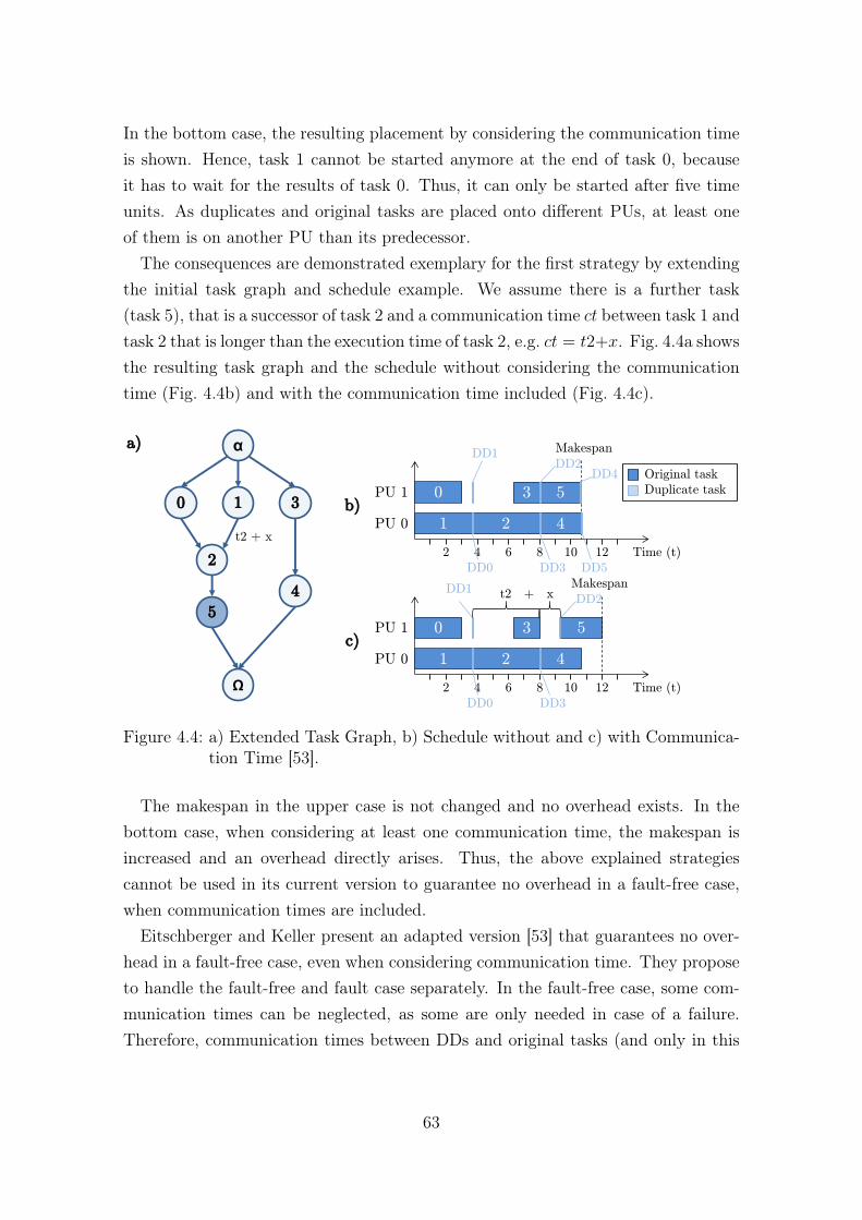
In the bottom case, the resulting placement by considering the communication timeis shown. Hence, task 1 cannot be started anymore at the end of task 0, becauseit has to wait for the results of task 0. Thus, it can only be started after five timeunits. As duplicates and original tasks are placed onto different PUs, at least oneof them is on another PU than its predecessor.

The consequences are demonstrated exemplary for the first strategy by extendingthe initial task graph and schedule example. We assume there is a further task(task 5), that is a successor of task 2 and a communication time ct between task 1 andtask 2 that is longer than the execution time of task 2, e.g. ct = t2+x. Fig. 4.4a showsthe resulting task graph and the schedule without considering the communicationtime (Fig. 4.4b) and with the communication time included (Fig. 4.4c).

5

5

2 PU 0

PU 1 3

Original task

Duplicate task

Time (t)

Makespan

2 4 6 8 10 12

0

1 4

DD4

DD0

DD2

DD3

α

0 1

2

3

4

Ω

a)

b)

c) 2 PU 0

PU 1 3

Time (t)

Makespan

2 4 6 8 10 12

0

1 4

DD0

DD2

DD3

DD1

5

t2 + x

DD5

DD1 t2 + x

Figure 4.4: a) Extended Task Graph, b) Schedule without and c) with Communica-tion Time [53].

The makespan in the upper case is not changed and no overhead exists. In thebottom case, when considering at least one communication time, the makespan isincreased and an overhead directly arises. Thus, the above explained strategiescannot be used in its current version to guarantee no overhead in a fault-free case,when communication times are included.

Eitschberger and Keller present an adapted version [53] that guarantees no over-head in a fault-free case, even when considering communication time. They proposeto handle the fault-free and fault case separately. In the fault-free case, some com-munication times can be neglected, as some are only needed in case of a failure.Therefore, communication times between DDs and original tasks (and only in this

63

order) are not considered in the fault-free case. With this extension, no overhead ina fault-free case can be guaranteed. Only in case of a failure, these communicationtimes have to be considered, because then some of the DDs are converted to Ds andexecuted. Hence, their results have to be sent to the successor tasks, which leads toa few more shifts of tasks in the fault case.

However, in the fault-free case DDs sometimes have to be placed during the run-time of original tasks on the same PU. Thus, there exist some overlapping of tasks.But as the information about a failure is known prior to the DD execution, theseoverlapping can be solved in the fault case. To support this behavior, each PU needsthe information about the complete task graph. A memory buffer is required to holdthe results of tasks that have finished, so that the transmission to successor taskson other PUs is continued in case of a failure. Fig. 4.5 illustrates the placement ofDDs for the old and for the new version.

5

Original task

Duplicate task

α

0 1

2

3

4

Ω

a)

b)

c)

2 PU 0

PU 1 3

Time (t)

Makespan

2 4 6 8 10 12

0

1 4

DD0

DD2

DD3

5

t2 + x

DD1 t2 + x

5

2

3

Time (t)

Makespan

2 4 6 8 10 12

0

1 4

DD4

DD0

DD2

DD3

DD1

DD5

PU 0

PU 1

Figure 4.5: a) Example Taskgraph, b) DD Placement Old Version, c) DD PlacementNew Version [53].

In Fig. 4.5b the old schedule with an overhead in a fault-free case is shown. InFig. 4.5c the new version is depicted. Here, an overlapping of DD2 and task 5 existsand the makespan remains constant.

An implementation of a corresponding scheduler that supports the above ex-plained duplicate placement strategies is presented by Eitschberger and Keller [53].The scheduler consists of two parts: One part for the schedule generation, i.e. theplacement of duplicates, the other for simulating the execution of a schedule in thefault-free and fault case to predict the overhead. The scheduler has various options

64

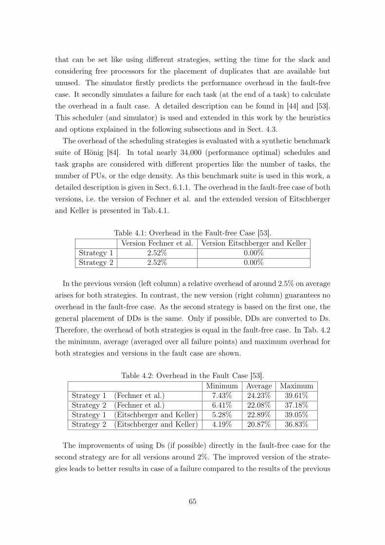
that can be set like using different strategies, setting the time for the slack andconsidering free processors for the placement of duplicates that are available butunused. The simulator firstly predicts the performance overhead in the fault-freecase. It secondly simulates a failure for each task (at the end of a task) to calculatethe overhead in a fault case. A detailed description can be found in [44] and [53].This scheduler (and simulator) is used and extended in this work by the heuristicsand options explained in the following subsections and in Sect. 4.3.

The overhead of the scheduling strategies is evaluated with a synthetic benchmarksuite of Hönig [84]. In total nearly 34,000 (performance optimal) schedules andtask graphs are considered with different properties like the number of tasks, thenumber of PUs, or the edge density. As this benchmark suite is used in this work, adetailed description is given in Sect. 6.1.1. The overhead in the fault-free case of bothversions, i.e. the version of Fechner et al. and the extended version of Eitschbergerand Keller is presented in Tab.4.1.

Table 4.1: Overhead in the Fault-free Case [53].Version Fechner et al. Version Eitschberger and Keller

Strategy 1 2.52% 0.00%Strategy 2 2.52% 0.00%

In the previous version (left column) a relative overhead of around 2.5% on averagearises for both strategies. In contrast, the new version (right column) guarantees nooverhead in the fault-free case. As the second strategy is based on the first one, thegeneral placement of DDs is the same. Only if possible, DDs are converted to Ds.Therefore, the overhead of both strategies is equal in the fault-free case. In Tab. 4.2the minimum, average (averaged over all failure points) and maximum overhead forboth strategies and versions in the fault case are shown.

Table 4.2: Overhead in the Fault Case [53].Minimum Average Maximum

Strategy 1 (Fechner et al.) 7.43% 24.23% 39.61%Strategy 2 (Fechner et al.) 6.41% 22.08% 37.18%Strategy 1 (Eitschberger and Keller) 5.28% 22.89% 39.05%Strategy 2 (Eitschberger and Keller) 4.19% 20.87% 36.83%

The improvements of using Ds (if possible) directly in the fault-free case for thesecond strategy are for all versions around 2%. The improved version of the strate-gies leads to better results in case of a failure compared to the results of the previous

65

version. While for the previous version the overhead is on average 24% for strat-egy 1 and 22% for strategy 2, the overhead of the improved version is around 1.3%lower. The maximum overhead of both versions is for all strategies nearly the same,but the minimum overhead is up to 2.2% lower in the improved version. The largedifference in general between the minimum and maximum overhead results from thetime at which a failure occurs. Is a failure directly in the beginning of a schedule,several duplicates have to be extended, tasks have to be shifted and a high overheadarises. In contrast, when a failure occurs shortly before the end of a schedule, onlyfew duplicates must be extended and fewer shifts must be performed. Therefore,the overhead in the latter situation is small.

In this work, only the new version proposed by Eitschberger and Keller is used forthe placement of Ds and DDs (Strategy 1 and 2). Therefore, no difference is madein the following between the versions.

4.2.2 Use Half PUs for Originals (UHPO)

A simple way to achieve a high FT is to use half of the available PUs for originaltasks and the other half for placing duplicates. In this case, the already existingschedule is not used anymore. Instead, a simple list scheduler generates a newschedule with the reduced number of PUs. A copy of the schedule can then beplaced onto the remaining PUs. Dependencies between original tasks and duplicatesare not considered, because both schedules are executed synchronously. Therefore,the performance of a schedule is not influenced in case of a failure. In Fig. 4.6 anexample schedule (upper case)2 and the resulting schedule by using this heuristic(bottom case) is illustrated.

In this example, all tasks are placed in sequence on one PU and the transfer timesbetween the tasks do not have to be considered anymore (bottom case). Thus, noparallelism is used anymore within the original schedule, because only two PUs areavailable. Instead, a copy of the sequential solution is placed on the other PU.This heuristic can only be used in the fault-free case, because only one failure isconsidered and thus no more duplicates have to be included in case of a failure. InLst. 5.1 a simplified code for the list scheduler is shown.

2For simplification, all following examples are related to this example schedule, if not declaredotherwise.

66

3 0 PU 0

PU 1 3

Original task

Duplicates

Time (t)

Old

makespan

2 4 6 8 10 12

1 2 0

14

New

makespan

2 1

PU 0

PU 1 3

Time (t)

Makespan

2 4 6 8 10 12

1

2 0 2 4

Figure 4.6: Example Schedule to Illustrate the Changes by the UHPO-option.

1 for(taskIndex = 0; taskIndex < numberOfTasks; taskIndex++) {2 earliestBeginning = -1;3 currentProcessor = beginProcessorList;4 halfProcessors = 0;5 while(currentProcessor != NULL && halfProcessors < numberOfProcessors/2)

{6 beginning = 0;7 for(j = 0; j < task[i].predecessornumber; j++)8 if(predec[i][j].processorindex != currentprocessor->processorindex)9 if(predec[i][j].finishtime + predec[i][j].transfertime > beginning)10 beginning = predec[i][j].finishtime + predec[i][j].transfertime;11 if(currentprocessor->task != NULL) {12 currenttask = currentprocessor->task;13 while(currenttask->next != NULL)14 currenttask = currenttask->next;15 if(currenttask->finishtime > beginning)16 beginning = currenttask->finishtime;17 }18 if(earliestBeginning == -1 || earliestBeginning > beginning) {19 earliestBeginning = beginning;20 bestProcessor = currentProcessor;21 }22 halfProcessors++;23 currentProcessor = currentProcessor->next;24 }25 createtask(...);26 inserttask(bestProcessor, earliestBeginning,...);27 }

Listing 4.1: Pseudo Code of the List Scheduler.

67

For each task (line 1) the earliest beginning is initially set to -1, the currentprocessor is the first processor in the processor list and halfProcessors is set tozero (lines 2 - 4). Then, for each processor of the first half (line 5) the beginningof the new task is set to zero (line 6). The list scheduler checks when the startingtime of the new task would be, because of the dependencies and transfer times ofthe predecessors (lines 7 - 10). If there exist tasks on the current processor (line 11),the finish time of the last task is compared with the beginning of the new task. Isthe finish time later, the beginning has to be corrected (lines 12 - 17). Thus, alsopredecessors that are placed on the current processor (without any transfer times)are considered. Then, the overall earliest beginning and the corresponding processorare corrected (lines 18 - 21), halfProcessors is incremented and the next processoris checked (lines 22 - 24). Finally, when half of the available processors are checked,the new task is created and inserted on the best processor with the earliest starttime (lines 25 - 27).

To place the duplicates, the best processor is fixed by using the processor indexfor the original task plus half of the processors. Thus, the duplicates are mapped inthe same way like the original tasks, but on the other half of the processors.

4.2.3 Excursion: Use Duplicates for Delayed Tasks

Static task duplication is typically used either to reduce communication costs or totolerate failures that occur during the runtime of a schedule. However, duplicatescan also be used in other situations to improve the performance of a schedule. Forexample as demonstrated by Eitschberger and Keller [53] in case of a performanceloss of a PU. Especially in grid systems, the owner of a PU might need a fraction ofthe computing power of a PU for other executions. In this case, the scheduled orig-inal task can only be executed with the remaining fraction of the computing power.Thus, the task is slowed down and the computation time is extended. When theexecution of a slowed original task becomes longer than executing the correspondingduplicate, it can be worthwhile to abort the original task and execute the duplicateinstead.

To handle such slowdowns, the completion time of the original task with the re-duced performance has to be calculated during the runtime and sent via a messageto the corresponding duplicate. Then, the predicted finish time of the duplicate canbe compared with the completion time of the slowed original task. If the duplicatecan finish earlier, an abort message is sent to the original task, otherwise the dupli-

68

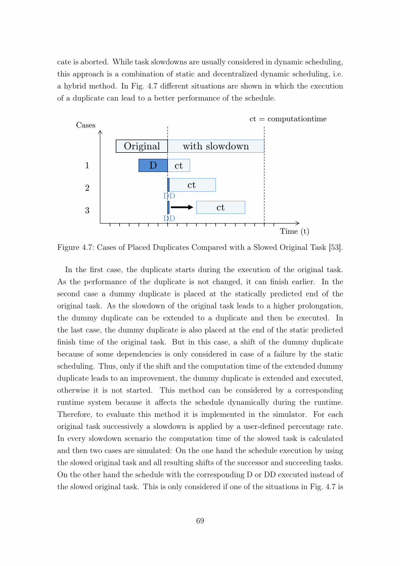
cate is aborted. While task slowdowns are usually considered in dynamic scheduling,this approach is a combination of static and decentralized dynamic scheduling, i.e.a hybrid method. In Fig. 4.7 different situations are shown in which the executionof a duplicate can lead to a better performance of the schedule.

Time (t)

ct = computationtime

3

2

1

with slowdown

ct

ct

D

Original

DD

ct DD

Cases

Figure 4.7: Cases of Placed Duplicates Compared with a Slowed Original Task [53].

In the first case, the duplicate starts during the execution of the original task.As the performance of the duplicate is not changed, it can finish earlier. In thesecond case a dummy duplicate is placed at the statically predicted end of theoriginal task. As the slowdown of the original task leads to a higher prolongation,the dummy duplicate can be extended to a duplicate and then be executed. Inthe last case, the dummy duplicate is also placed at the end of the static predictedfinish time of the original task. But in this case, a shift of the dummy duplicatebecause of some dependencies is only considered in case of a failure by the staticscheduling. Thus, only if the shift and the computation time of the extended dummyduplicate leads to an improvement, the dummy duplicate is extended and executed,otherwise it is not started. This method can be considered by a correspondingruntime system because it affects the schedule dynamically during the runtime.Therefore, to evaluate this method it is implemented in the simulator. For eachoriginal task successively a slowdown is applied by a user-defined percentage rate.In every slowdown scenario the computation time of the slowed task is calculatedand then two cases are simulated: On the one hand the schedule execution by usingthe slowed original task and all resulting shifts of the successor and succeeding tasks.On the other hand the schedule with the corresponding D or DD executed instead ofthe slowed original task. This is only considered if one of the situations in Fig. 4.7 is

69

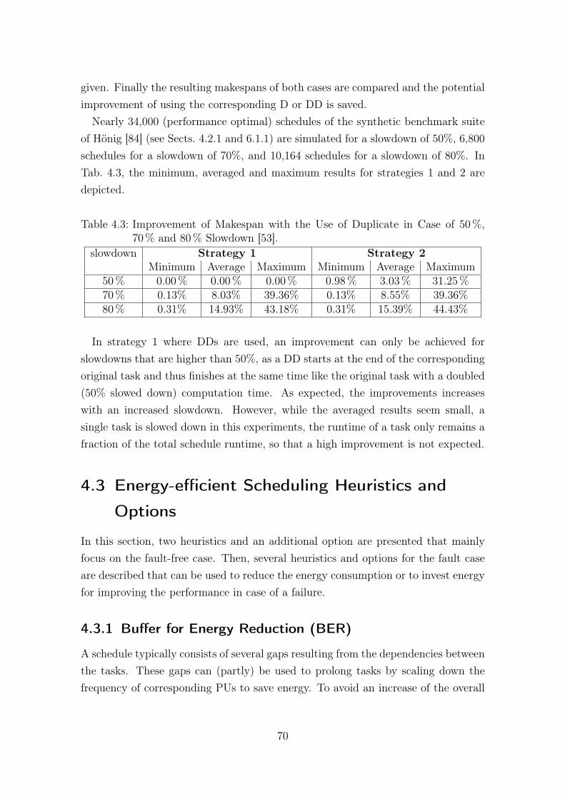
given. Finally the resulting makespans of both cases are compared and the potentialimprovement of using the corresponding D or DD is saved.

Nearly 34,000 (performance optimal) schedules of the synthetic benchmark suiteof Hönig [84] (see Sects. 4.2.1 and 6.1.1) are simulated for a slowdown of 50%, 6,800schedules for a slowdown of 70%, and 10,164 schedules for a slowdown of 80%. InTab. 4.3, the minimum, averaged and maximum results for strategies 1 and 2 aredepicted.

Table 4.3: Improvement of Makespan with the Use of Duplicate in Case of 50%,70% and 80% Slowdown [53].

slowdown Strategy 1 Strategy 2Minimum Average Maximum Minimum Average Maximum

50% 0.00% 0.00% 0.00% 0.98% 3.03% 31.25%70% 0.13% 8.03% 39.36% 0.13% 8.55% 39.36%80% 0.31% 14.93% 43.18% 0.31% 15.39% 44.43%

In strategy 1 where DDs are used, an improvement can only be achieved forslowdowns that are higher than 50%, as a DD starts at the end of the correspondingoriginal task and thus finishes at the same time like the original task with a doubled(50% slowed down) computation time. As expected, the improvements increaseswith an increased slowdown. However, while the averaged results seem small, asingle task is slowed down in this experiments, the runtime of a task only remains afraction of the total schedule runtime, so that a high improvement is not expected.

4.3 Energy-efficient Scheduling Heuristics and

Options

In this section, two heuristics and an additional option are presented that mainlyfocus on the fault-free case. Then, several heuristics and options for the fault caseare described that can be used to reduce the energy consumption or to invest energyfor improving the performance in case of a failure.

4.3.1 Buffer for Energy Reduction (BER)

A schedule typically consists of several gaps resulting from the dependencies betweenthe tasks. These gaps can (partly) be used to prolong tasks by scaling down thefrequency of corresponding PUs to save energy. To avoid an increase of the overall

70

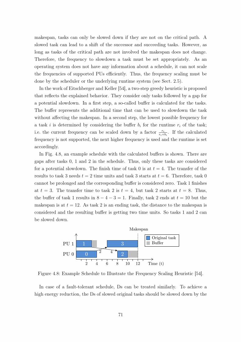
makespan, tasks can only be slowed down if they are not on the critical path. Aslowed task can lead to a shift of the successor and succeeding tasks. However, aslong as tasks of the critical path are not involved the makespan does not change.Therefore, the frequency to slowdown a task must be set appropriately. As anoperating system does not have any information about a schedule, it can not scalethe frequencies of supported PUs efficiently. Thus, the frequency scaling must bedone by the scheduler or the underlying runtime system (see Sect. 2.5).

In the work of Eitschberger and Keller [54], a two-step greedy heuristic is proposedthat reflects the explained behavior. They consider only tasks followed by a gap fora potential slowdown. In a first step, a so-called buffer is calculated for the tasks.The buffer represents the additional time that can be used to slowdown the taskwithout affecting the makespan. In a second step, the lowest possible frequency fora task i is determined by considering the buffer bi for the runtime ri of the task;i.e. the current frequency can be scaled down by a factor ri

ri+bi. If the calculated

frequency is not supported, the next higher frequency is used and the runtime is setaccordingly.

In Fig. 4.8, an example schedule with the calculated buffers is shown. There aregaps after tasks 0, 1 and 2 in the schedule. Thus, only these tasks are consideredfor a potential slowdown. The finish time of task 0 is at t = 4. The transfer of theresults to task 3 needs t = 2 time units and task 3 starts at t = 6. Therefore, task 0cannot be prolonged and the corresponding buffer is considered zero. Task 1 finishesat t = 3. The transfer time to task 2 is t = 4, but task 2 starts at t = 8. Thus,the buffer of task 1 results in 8− 4− 3 = 1. Finally, task 2 ends at t = 10 but themakespan is at t = 12. As task 2 is an ending task, the distance to the makespan isconsidered and the resulting buffer is getting two time units. So tasks 1 and 2 canbe slowed down.

PU 0

PU 1 3

Original task

Buffer

Time (t)

Makespan

2 4 6 8 10 12

1

2 0 2 4

Figure 4.8: Example Schedule to Illustrate the Frequency Scaling Heuristic [54].

In case of a fault-tolerant schedule, Ds can be treated similarly. To achieve ahigh energy reduction, the Ds of slowed original tasks should be slowed down by the

71

same frequency. Thus, a buffer of an original task is reduced to the length of thecorresponding duplicate buffer, if that is shorter. Buffers of successor and succeedingtasks can also be used to extend the buffer of an original task by shifting the tasksaccordingly. DDs, in contrast, are not considered for a prolongation, because theyare placed with runtime zero. Therefore, these are not executed in a fault-free case.They can only be shifted. For all remaining gaps the frequencies of the PUs can bescaled down for further savings to the lowest supported frequency, i.e. to the idlefrequency. This heuristic is related to the fault-free case. However, it is indirectlyalso used in the fault case, e.g. in the EP-heuristic explained in the following. InLst. 4.2 the pseudo code of the heuristic is presented.

1 Set all task->buffers to 0;2 helpbuffer = 0;3 gap = task->finishtime until next original task->starttime4 for(all tasks followed by a gap) {5 if(successor tasks exist)6 task->buffer = min(distance to all successors - transfer times);7 else {8 if(task is an ending task)9 task->buffer = makespan - task->finishtime;10 else11 task->buffer = gap;12 }13 }14 for(all Ds, where original task->buffer > 0) {15 if(D task->buffer < original task->buffer)16 original task->buffer = D task->buffer;17 helpbuffer = original task->buffer;1819 while(Ds exist in the gap (original PU))20 consider all D task->buffers, reduce helpbuffer;21 while(Ds exist in the gap (D PU))22 consider all D task->buffers, reduce helpbuffer;23 if(helpbuffer > 0) {24 find the best frequency to fill the helpbuffer;25 reduce the helpbuffer if necessary;26 }2728 if(helpbuffer > 0) {29 while(gap beginning is not reached (D PU), go backwards)30 shift all Ds in the gap, reduce their buffers;31 change/shift the D infront of the gap itself, reduce its buffer;32 while(gap beginning is not reached (original PU), go backwards)33 shift all Ds in the gap, reduce their buffers;34 change the original task infront of the gap, reduce its buffer;35 }36 }

Listing 4.2: Pseudo Code of BER-heuristic.

72

The buffers of all tasks and the help buffer are initially set to zero (lines 1 - 2). Inevery case, where a gap is after a task, i.e. the finish time of a task is smaller thanthe beginning of the next original task, its buffer is firstly set either according to theminimum time, that can be used without shifting successor tasks, or to the gap size(lines 3 - 13). Thus, also duplicates3 within a gap can have a buffer bigger than zero.Secondly, to avoid shiftings as a result of duplicates, the buffers of all original tasksare reduced to its corresponding duplicate buffers, if the duplicate buffers are smallerand the help buffer is always set to the original task buffer (lines 14 - 18). Then, thegaps between original tasks are checked. If there exist duplicates within a gap, thesebuffers are considered to keep the buffer size of the original task before the gap aslarge as possible (lines 19 - 20). Therefore, if a duplicate within a gap has a bufferand the beginning of the duplicate lies within the buffer of the original task beforethe gap, the duplicate could be shifted for the time of its own buffer. The beginningof the duplicate can then be used as restriction for the buffer of the original taskand afterwards the duplicate buffer can be reduced for the time of the shifting. Thisprocedure can be repeated for all duplicates within a gap until the next originaltask starts. The overall resulting buffer is saved in the help buffer. In the same way,the duplicates within the gap on the corresponding duplicate PU are considered(lines 21 - 22). The calculation of the overall buffer and the resulting shifting of allduplicates within a gap (and the reduction of their buffers) is separated in two whileloops (lines 19 and 32 for the original task and lines 21 and 29 for the duplicatetask), because only if the overall buffer, i.e. the help buffer, is higher than zero, anyduplicate must be shifted. The buffer is then used to find the best frequency. Afrequency is selected to fill the help buffer as much as possible by slowing down thetask. If the help buffer cannot be filled completely, it is reduced to be filled by usingthe next higher supported frequency (lines 23 - 26). At the end, if the help bufferis still bigger than zero (line 28), all duplicates within the gaps can be correctedbackwards from the end of the gap. Finally, the buffer and properties of the originaltask and its corresponding duplicate before the gap are corrected (lines 29 - 36).

Tasks are typically placed as early as possible in a schedule, so that only gapsafter tasks must be considered. However, in general also buffers before tasks arepossible, when tasks are placed later like task 2 in Fig. 4.8. The calculation of thesebuffers and the corresponding frequencies of tasks can then be done in a similar way,but from the end of a gap to the beginning. This leads to different frequencies and adifference in energy consumption. While the consideration of both buffers, i.e. before

3In this context, the term duplicates is used for Ds and DDs.

73

a task and after a task, can lead to better results, a much more complex algorithmand a longer scheduling time is necessary to find optimized solutions. A decisionabout using a buffer then also influences the buffer usage of other tasks, i.e. thestarting (and ending) times of tasks, which results in several additional solutions tobe checked. As in the synthetic benchmark suite used in Sect. 6.1.1 tasks are alwaysplaced as early as possible, the BER-heuristic is restricted to such cases. Therefore,buffers before tasks are not considered.

4.3.2 Option: Insert Order (SDE vs. SED)

When considering both fault tolerance by duplicates and heuristics to reduce en-ergy consumption like BER, the insert order can have a significant influence on theoptimization. While placing the duplicates first and reduce the energy afterwardsimproves the FT, the vice versa handling, in contrast, can result in a lower energyconsumption. Therefore, the user can select the order SED (Scheduling → Energy→ Duplicates) and SDE (Scheduling → Duplicates → Energy). In Fig. 4.9 bothsituations are illustrated based on the initial example.

DD3

Original task

Duplicate task

Slowed task

PU 0

3

Time (t)

Makespan

2 4 6 8 10 12

0 2 4

PU 1

Makespan

DD0 DD1 DD2

0

PU 0

3

Time (t) 2 4 6 8 10 12

1

2 0 2 4

PU 1

DD1 DD2

3

SED:

SDE:

1

2

Figure 4.9: Example Schedule to Illustrate the Changes by the Insert Order [54].

In the upper case (SED), the original tasks are slowed down first by the BER-heuristic to reduce the energy. Then, the duplicates are included. Thus, tasks 1and 2 are slowed down by using a lower frequency and only DDs can be placed forall tasks. In contrast, in the bottom case (SDE) the duplicates are placed first.

74

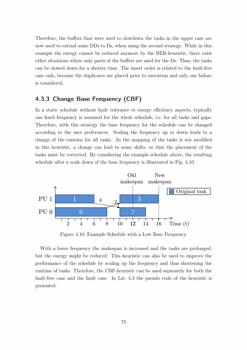
Therefore, the buffers that were used to slowdown the tasks in the upper case arenow used to extend some DDs to Ds, when using the second strategy. While in thisexample the energy cannot be reduced anymore by the BER-heuristic, there existother situations where only parts of the buffers are used for the Ds. Thus, the taskscan be slowed down for a shorter time. The insert order is related to the fault-freecase only, because the duplicates are placed prior to execution and only one failureis considered.

4.3.3 Change Base Frequency (CBF)

In a static schedule without fault tolerance or energy efficiency aspects, typicallyone fixed frequency is assumed for the whole schedule, i.e. for all tasks and gaps.Therefore, with this strategy the base frequency for the schedule can be changedaccording to the user preferences. Scaling the frequency up or down leads to achange of the runtime for all tasks. As the mapping of the tasks is not modifiedin this heuristic, a change can lead to some shifts, so that the placement of thetasks must be corrected. By considering the example schedule above, the resultingschedule after a scale down of the base frequency is illustrated in Fig. 4.10.

PU 0

PU 1 3

Original task

Time (t)

New

makespan

2 4 6 8 10 12

1

2 0

2 4

12 14 16

Old

makespan

Figure 4.10: Example Schedule with a Low Base Frequency.

With a lower frequency the makespan is increased and the tasks are prolonged,but the energy might be reduced. This heuristic can also be used to improve theperformance of the schedule by scaling up the frequency and thus shortening theruntime of tasks. Therefore, the CBF-heuristic can be used separately for both thefault-free case and the fault case. In Lst. 4.3 the pseudo code of the heuristic ispresented.

75

1 readschedulefile(...);2 createsprocessorlist(...);3 for(all tasks){4 newtask = createtask(...);5 inserttaskinprocessorlist(...);6 }7 for(all tasks){8 change properties of the task;9 shift(...);10 }

Listing 4.3: Pseudo Code of CBF-heuristic.

Initially, the already existing schedule (and task graph) file is read (line 1). Aprocessor list with the number of PUs is created (line 2). Then, all tasks are createdand inserted in the processor list on the corresponding PU (lines 3 - 6). Until now,the schedule is created as given by the schedule and task graph file.

Then, for all tasks the properties are adapted by changing the base frequency tothe frequency (level) given by a user (lines 7 - 8). Firstly, the computation timeand the finish time of a task are changed. Secondly, the frequency used is saved.Finally, the energy consumption is re-calculated with the new frequency. After allproperties are adapted, the successor and succeeding tasks are shifted according tothe prolongation or shortening of a task or according to the dependencies betweenthe tasks (lines 10 - 11). The mapping of the tasks is, therefore, not changed.Only the beginning and ending of the tasks are modified. Gaps within a scheduleare sometimes filled by the prolongation of tasks and often new gaps arise by theresulting shifts of other tasks.

4.3.4 Energy for Performance (EP)

A failure of a PU during the runtime of a schedule typically leads to a performanceoverhead. While in a fault-free case the focus might be on the energy, this couldchange in case of a failure. Then, a fast termination of a schedule can be preferable.As demonstrated by Eitschberger and Keller [54], energy can be invested to improvethe performance of a schedule in case of a failure by scaling up frequencies andthus speeding up the execution of tasks. One possibility is to consider all Ds andDDs that have to be extended due to the failure and calculate for each of thesetasks a higher frequency that can be used to reduce or totally undo the resultingoverhead. When the calculated frequency for a task is not supported by the system,the next higher or the highest possible frequency is used instead. In this heuristic,

76

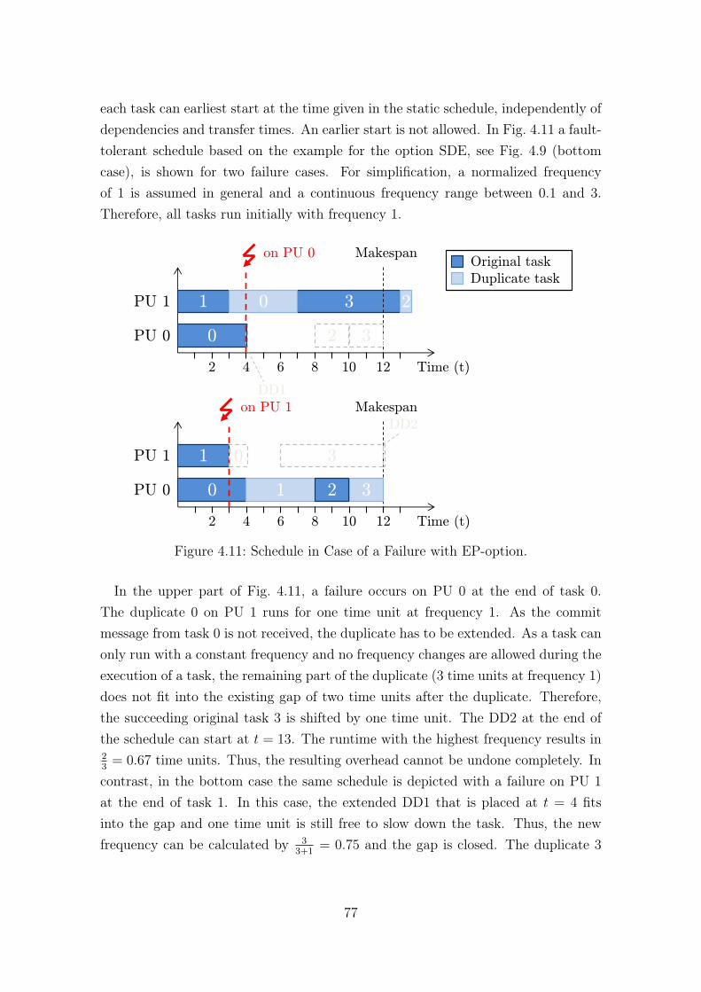
each task can earliest start at the time given in the static schedule, independently ofdependencies and transfer times. An earlier start is not allowed. In Fig. 4.11 a fault-tolerant schedule based on the example for the option SDE, see Fig. 4.9 (bottomcase), is shown for two failure cases. For simplification, a normalized frequencyof 1 is assumed in general and a continuous frequency range between 0.1 and 3.Therefore, all tasks run initially with frequency 1.

Original task

Duplicate task

Makespan

PU 0

3

Time (t) 2 4 6 8 10 12

1

2 0

PU 1

DD1

3

0 2

on PU 0

Makespan

PU 0

3

Time (t) 2 4 6 8 10 12

1

0

PU 1

1

on PU 1

3

DD2

2

0

Figure 4.11: Schedule in Case of a Failure with EP-option.

In the upper part of Fig. 4.11, a failure occurs on PU 0 at the end of task 0.The duplicate 0 on PU 1 runs for one time unit at frequency 1. As the commitmessage from task 0 is not received, the duplicate has to be extended. As a task canonly run with a constant frequency and no frequency changes are allowed during theexecution of a task, the remaining part of the duplicate (3 time units at frequency 1)does not fit into the existing gap of two time units after the duplicate. Therefore,the succeeding original task 3 is shifted by one time unit. The DD2 at the end ofthe schedule can start at t = 13. The runtime with the highest frequency results in23= 0.67 time units. Thus, the resulting overhead cannot be undone completely. In

contrast, in the bottom case the same schedule is depicted with a failure on PU 1at the end of task 1. In this case, the extended DD1 that is placed at t = 4 fitsinto the gap and one time unit is still free to slow down the task. Thus, the newfrequency can be calculated by 3

3+1= 0.75 and the gap is closed. The duplicate 3

77

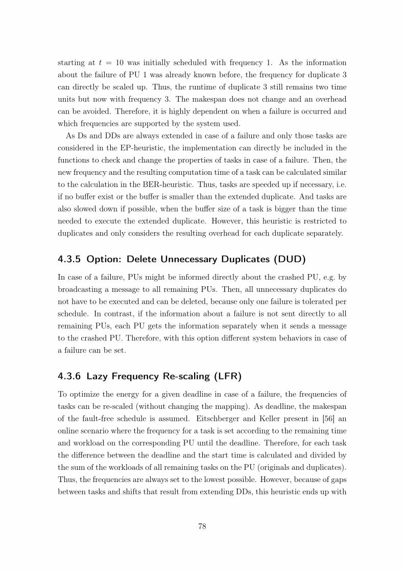
starting at t = 10 was initially scheduled with frequency 1. As the informationabout the failure of PU 1 was already known before, the frequency for duplicate 3can directly be scaled up. Thus, the runtime of duplicate 3 still remains two timeunits but now with frequency 3. The makespan does not change and an overheadcan be avoided. Therefore, it is highly dependent on when a failure is occurred andwhich frequencies are supported by the system used.

As Ds and DDs are always extended in case of a failure and only those tasks areconsidered in the EP-heuristic, the implementation can directly be included in thefunctions to check and change the properties of tasks in case of a failure. Then, thenew frequency and the resulting computation time of a task can be calculated similarto the calculation in the BER-heuristic. Thus, tasks are speeded up if necessary, i.e.if no buffer exist or the buffer is smaller than the extended duplicate. And tasks arealso slowed down if possible, when the buffer size of a task is bigger than the timeneeded to execute the extended duplicate. However, this heuristic is restricted toduplicates and only considers the resulting overhead for each duplicate separately.

4.3.5 Option: Delete Unnecessary Duplicates (DUD)

In case of a failure, PUs might be informed directly about the crashed PU, e.g. bybroadcasting a message to all remaining PUs. Then, all unnecessary duplicates donot have to be executed and can be deleted, because only one failure is tolerated perschedule. In contrast, if the information about a failure is not sent directly to allremaining PUs, each PU gets the information separately when it sends a messageto the crashed PU. Therefore, with this option different system behaviors in case ofa failure can be set.

4.3.6 Lazy Frequency Re-scaling (LFR)

To optimize the energy for a given deadline in case of a failure, the frequencies oftasks can be re-scaled (without changing the mapping). As deadline, the makespanof the fault-free schedule is assumed. Eitschberger and Keller present in [56] anonline scenario where the frequency for a task is set according to the remaining timeand workload on the corresponding PU until the deadline. Therefore, for each taskthe difference between the deadline and the start time is calculated and divided bythe sum of the workloads of all remaining tasks on the PU (originals and duplicates).Thus, the frequencies are always set to the lowest possible. However, because of gapsbetween tasks and shifts that result from extending DDs, this heuristic ends up with

78

high frequencies close to the deadline and is, therefore, called lazy. This heuristic isonly related to the fault case.

Consider the initial example schedule and a failure on PU1 at the end of task 1,similar to the example in Fig. 4.11 bottom case. In Fig. 4.12 upper case, the sched-ule is depicted without any frequency scaling. An overhead of four time units ispresent. For simplification, a normalized frequency of 1 is assumed in general anda continuous frequency range between 0.1 and 3. Therefore, all tasks run initiallywith frequency 1.

Original task

Duplicate task

2

Makespan

PU 0

3

Time (t) 2 4 6 8 10 12

1

0

PU 1

1

on PU 1

3

DD2

2

0

1 3

1.375 1.375

2

Frequency

3

Time (t) 2 4 6 8 10 12

1

0

PU 1

DD2

PU 0

1

0

2

1.375

Figure 4.12: Example Schedule to Illustrate the Changes by the LFR-heuristic.

In the bottom case of Fig 4.12, the lazy frequency scaling is shown. In the fault-free case, all tasks are running with the normalized frequency 1. At time unit 4the duplicate of task 1 on PU 0 has to be executed. Now, to calculate the newfrequency, the sum of the remaining task workloads on this PU is divided by theremaining time until the deadline, i.e. 3+2+6

12−4 = 118= 1.375. Duplicate 1 is executed

with a frequency of 1.375. As in this example only two PUs exist (where one PUhas failed) no transfer time is considered, because all remaining tasks must run onPU 0. In contrast to the EP-heuristic (where each task can earliest start at the timegiven by the static schedule), the tasks are allowed to start when all results of thepredecessors are available. Therefore, tasks are not only shifted forward but alsosometimes backwards if possible. Hence, task 2 can directly be started after D1 andalso task 3 after task 2 with a frequency of 1.375 and without any overhead.

79

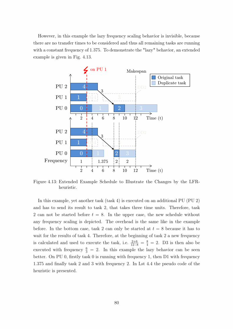
However, in this example the lazy frequency scaling behavior is invisible, becausethere are no transfer times to be considered and thus all remaining tasks are runningwith a constant frequency of 1.375. To demonstrate the "lazy" behavior, an extendedexample is given in Fig. 4.13.

Original task

Duplicate task

2

Makespan

PU 0

3

Time (t) 2 4 6 8 10 12

1

0

PU 1

1

on PU 1

3

DD2

2

0

1 3

1.375 2

2

Frequency

3

Time (t) 2 4 6 8 10 12

1

0

PU 1

DD2

PU 0

1

0

2

2

PU 2 4 3

PU 2 4

4

4

3

Figure 4.13: Extended Example Schedule to Illustrate the Changes by the LFR-heuristic.

In this example, yet another task (task 4) is executed on an additional PU (PU 2)and has to send its result to task 2, that takes three time units. Therefore, task2 can not be started before t = 8. In the upper case, the new schedule withoutany frequency scaling is depicted. The overhead is the same like in the examplebefore. In the bottom case, task 2 can only be started at t = 8 because it has towait for the results of task 4. Therefore, at the beginning of task 2 a new frequencyis calculated and used to execute the task, i.e. 2+6

12−8 = 84= 2. D3 is then also be

executed with frequency 63= 2. In this example the lazy behavior can be seen

better. On PU 0, firstly task 0 is running with frequency 1, then D1 with frequency1.375 and finally task 2 and 3 with frequency 2. In Lst 4.4 the pseudo code of theheuristic is presented.

80

1 Task *currenttask = NULL;2 currenttask = task;34 while(currenttask != NULL){5 if(currenttask is an original or a duplicate that has to be executed)6 totalworkload = totalworkload + currenttask->comptime;7 currenttask = currenttask->next;8 }910 newfreq = totalworkload/(makespan - task->starttime);11 task->finishtime = task->starttime + task->comptime * task->freq/newfreq;12 task->comptime = task->comptime * task->freq/newfreq;13 task->freq = newfreq;14 task->energyconsumption = setenergy(...);15 check if adapted properties influence position of successor tasks;16 check if adapted properties influence position of succeeding tasks;

Listing 4.4: Pseudo Code of LFR-heuristic.

In the beginning, a pointer currenttask is created and initialized with the taskto be considered (lines 1 - 3). Then, the total workload of all succeeding tasks thathave to be executed is summed up (lines 4 - 9). The new frequency for the task isthe total workload divided by the time until the makespan (line 10). The finish andcomputation times of the task are calculated based on the new frequency (lines 11- 12). The new frequency is saved as task frequency and the energy consumptionfor the task is calculated (lines 13 - 14). Finally, the influences on successor andsucceeding tasks of the adapted task are checked and changed if necessary (lines 15- 16).

In contrast to the EP-heuristic, that only focuses on the overhead for each du-plicate, the LFR-heuristic only considers the total workload of a PU to find a newfrequency. Thus, neither the overhead of a task nor the dependencies between tasksare considered.

4.3.7 Constant Power (CP)

Another approach to re-scale the frequencies of tasks in case of a failure is the so-called CP-heuristic, demonstrated by Eitschberger and Keller [56]. This heuristicis based on the approximation algorithm from Pruhs et al. [147] (see Sect. 3.1.2).To obtain an energy-optimal solution, the power consumptions of all PUs are keptconstant. Therefore, the frequency of a PU is set according to the fraction of thepower budget that is related to the PU. This fraction changes with the numberof PUs that are executing tasks at the same time. While several distributions of

81

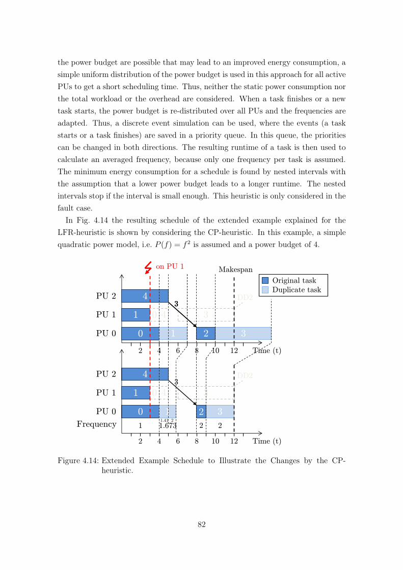
the power budget are possible that may lead to an improved energy consumption, asimple uniform distribution of the power budget is used in this approach for all activePUs to get a short scheduling time. Thus, neither the static power consumption northe total workload or the overhead are considered. When a task finishes or a newtask starts, the power budget is re-distributed over all PUs and the frequencies areadapted. Thus, a discrete event simulation can be used, where the events (a taskstarts or a task finishes) are saved in a priority queue. In this queue, the prioritiescan be changed in both directions. The resulting runtime of a task is then used tocalculate an averaged frequency, because only one frequency per task is assumed.The minimum energy consumption for a schedule is found by nested intervals withthe assumption that a lower power budget leads to a longer runtime. The nestedintervals stop if the interval is small enough. This heuristic is only considered in thefault case.

In Fig. 4.14 the resulting schedule of the extended example explained for theLFR-heuristic is shown by considering the CP-heuristic. In this example, a simplequadratic power model, i.e. P (f) = f 2 is assumed and a power budget of 4.

0 1

4

Original task

Duplicate task

2

Makespan

PU 0

3

Time (t) 2 4 6 8 10 12

1

0

PU 1

1

on PU 1

3

DD2

2

0

3 1.41 2

2

2

Frequency

3

Time (t) 2 4 6 8 10 12

1 PU 1

DD2

PU 0

1

0

2

PU 2 4 3

PU 2

4

4

3 3

3

2

1.673

Figure 4.14: Extended Example Schedule to Illustrate the Changes by the CP-heuristic.

82

A failure of PU 1 occurs at the end of task 1. As task 0 and task 4 are running atthis time, the frequencies of both tasks are not changed by the CP-heuristic, becauseonly one frequency per task is allowed. At t = 4 the duplicate of task 1 can start onPU 0. As two PUs are active at this event, the resulting frequency f for PU 0 can becalculated by f =

√power budgetactive PUs =

√42≈ 1.414 and the new runtime of duplicate 1

results in 2.12 time units. At t = 5, task 4 is finished so that the power budgetcan be completely used by PU 0 with a frequency of 2. Thus, the remaining part ofduplicate 1, i.e. (2.12−1) = 1.12 time units at frequency 1.414 can be executed withthe higher frequency. The overall runtime of duplicate 1 is then 1+ 1.12·1.414

2= 1.793

and the average frequency for duplicate 1 is 31.793

≈ 1.673. All remaining tasks onPU 0 are running with a frequency of 2, because PU 0 is the only active PU untilthe end. In Lst. 4.5 the pseudo code of the heuristic is presented.

1 while(there are tasks to be executed){2 PU = nextevent(...);34 if(PU is not activated){ // A new task starts5 activate PU;6 activePUs++;7 oldfrequency = newfrequency;8 newfrequency = sqrt(totalpowerbudget/activePUs);9 for(all PUs)10 if(PU is activated and task starts after or at failure)11 adapt remaining runtime according to the new frequency;12 timestamp = task start time;13 }14 else{ // A task finishes15 deactivate PU;16 activePUs--;17 oldfrequency = newfrequency;18 newfrequency = sqrt(totalpowerbudget/activePUs);19 for(all PUs)20 if(PU is activated and task starts after or at failure)21 adapt remaining runtime according to the new frequency;22 timestamp = task finish time;23 take next task on PU;24 }25 }2627 for(all tasks){28 calculate average frequency according to the runtime;29 set energy for task;30 }3132 calculate makespan;33 return(makespan);

Listing 4.5: Pseudo Code of CP-heuristic.

83

As long as there are tasks to be executed (line 1):

• Find the PU with the next event, i.e. where the next task starts or finishes.In the function nextevent(..) unconsidered duplicates are deleted if theDUD-option is set (line 2).

• If a new task starts (line 4), the corresponding PU is activated and the activenumber of PUs is incremented (lines 5 - 6). Then, the old and new frequenciesare set (lines 7 - 8). The tasks (after or at the failure) of all active PUs,including the PU with the new started task are considered to change theremaining runtime according to the new frequency (lines 9 - 11). Finally, thetime stamp is updated with the tasks’ starting time (lines 12 - 13).

• If a task finishes (lines 14), the procedure is similar to the above explained.First, the corresponding PU is deactivated and the number of active PUs isdecremented (lines 15 - 16). The frequencies are set and the runtimes of theactive tasks excluding the finished task are adapted (lines 17 - 21). The timestamp is set to the finish time of the task. The next task is chosen. In bothcases, i.e. a task starts or finishes, the old frequency and the time stamp arenecessary to determine the previous time interval with the old frequency forthe calculation of the remaining runtime with the new frequency.

After all tasks are completed, an average frequency for each task and the corre-sponding energy is calculated according to the adapted runtime of a task (lines 27 -30). Then, the makespan of the schedule is calculated and returned (lines 31 - 33).Thus, a resulting makespan and the corresponding schedule is given.

An optimized solution can now be found by using nested intervals. Starting witha maximum power budget PBmax = f 2

max · PUs, i.e. all PUs are running with thehighest frequency fmax. If the makespan of a schedule by using the CP-heuristicis higher than the makespan in a fault-free case, a solution is infeasible and thenested intervals stop. Otherwise, the mean power budget of the interval betweenthe maximum power budget and the minimum power budget PBmin = f 2

min · PUs,i.e. all PUs are running with the lowest frequency fmin, is chosen. Then, the intervalis halved in each step and the new mean power budget is calculated. If the makespanis higher than the makespan in a fault-free case, the minimum power budget is set tothe mean power budget, otherwise the maximum power budget is set to this value.The nested intervals end, when either the makespan of the schedule by using the

84

CP-heuristic mcp is close to the makespan m in a fault-free case, i.e. |mcp −m| ≤ ε,where ε = 0.001, or when mcp does not change anymore between two steps.

4.3.8 Option: Maximum Makspan Increase (MMI)

As the static task scheduling is done prior to execution (see Sect. 2.3.1), the makespanis already known when the schedule starts. A crash of a PU during the runtime ofa schedule usually leads to an overhead, i.e. a makespan increase. To undo theoverhead or at least to keep it small, the tasks can be accelerated by scaling up thefrequencies as much as possible. However, a small prolongation in case of a failurecan basically be acceptable for a user. Therefore, a maximum makespan increase tobe tolerable can be set as a percentage value to restrict the overhead and thus toscale up frequencies only in a moderate fashion. As demonstrated by Eitschbergerand Keller [56], a given maximum makespan increase in case of a failure often re-sults in a lower energy consumption. In some cases, the energy consumption for thefaulty schedule even becomes lower than for its corresponding fault-free variant whenconsidering an increased makespan. This option can only be used in combinationwith the two heuristics LFR and CP explained above. Otherwise, the maximummakespan increase is set to zero percent and thus switched off.

4.4 User Preferences and Corresponding Strategies

As seen in Chap. 3, an overall solution for the trade-off between PE, FT and E doesnot exist. A solution is very situational and highly depends on the user preferences.The focus can change for different systems and between the fault-free and faultcase. Often more than one criterion are important for a "good" solution. Next tothis fact, it is hardly possible to rate the preferences of a user in a general waylike using a percentage value for the different criteria. Instead, several strategiesshould be provided by the scheduler to reflect the preferences of a user in detail.Therefore, in this section firstly valid combinations of the above explained heuristicsand options are discussed. Secondly, combined strategies for the fault-free and faultcase are proposed. The strategies have been developed and integrated in the existingscheduler.

85

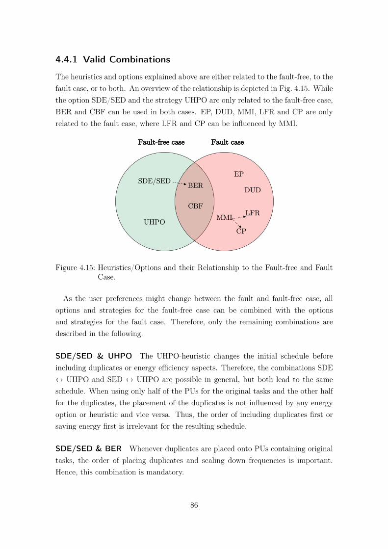
4.4.1 Valid Combinations

The heuristics and options explained above are either related to the fault-free, to thefault case, or to both. An overview of the relationship is depicted in Fig. 4.15. Whilethe option SDE/SED and the strategy UHPO are only related to the fault-free case,BER and CBF can be used in both cases. EP, DUD, MMI, LFR and CP are onlyrelated to the fault case, where LFR and CP can be influenced by MMI.

BER

CBF

SDE/SED

UHPO

EP

DUD

MMI LFR

Fault-free case Fault case

CP

Figure 4.15: Heuristics/Options and their Relationship to the Fault-free and FaultCase.

As the user preferences might change between the fault and fault-free case, alloptions and strategies for the fault-free case can be combined with the optionsand strategies for the fault case. Therefore, only the remaining combinations aredescribed in the following.

SDE/SED & UHPO The UHPO-heuristic changes the initial schedule beforeincluding duplicates or energy efficiency aspects. Therefore, the combinations SDE↔ UHPO and SED ↔ UHPO are possible in general, but both lead to the sameschedule. When using only half of the PUs for the original tasks and the other halffor the duplicates, the placement of the duplicates is not influenced by any energyoption or heuristic and vice versa. Thus, the order of including duplicates first orsaving energy first is irrelevant for the resulting schedule.

SDE/SED & BER Whenever duplicates are placed onto PUs containing originaltasks, the order of placing duplicates and scaling down frequencies is important.Hence, this combination is mandatory.

86

SDE/SED & CBF The insert position of a duplicate depends on the structure of aschedule, i.e. on the distribution of gaps and on the dependencies between tasks. Asoriginal tasks are prolonged or shortened and often shifted when changing the basefrequency, some gaps would be closed, others might arise. Thus, an initial placementof duplicates before using the CBF-heuristic would lead to further overhead thatcould be avoided when using the CBF-heuristic first. Therefore, the CBF-heuristichas to be considered initially. Afterwards the SDE/SED-option can be used forfurther savings. Hence, a combination of both is possible, but the SDE/SED-optionexclude the change of the base frequency.

UHPO & BER This combination is possible, too. First, the UHPO-heuristic isused to re-schedule the original tasks. After that, the BER-heuristic takes place.As explained above, the BER-heuristic has to be considered together with theSED/SDE-option.

UHPO and CBF In general, using half of the PUs for originals and changing thebase frequency can be used together. In this case, initially the original tasks arere-scheduled onto half of the PUs. Afterwards the base frequency is changed beforeincluding the duplicates.

BER- & All Heuristics for the Fault Case The BER-heuristic can be combinedwith all fault strategies. However, the frequencies for duplicates resulting from theBER-heuristic are changed whenever the user focus on another direction in caseof a failure. This means: By using any heuristic, the frequencies of duplicates arechanged according to the heuristic in use.

CBF & All Heuristics for the Fault Case The CBF-heuristic can be combinedwith the heuristics for the fault case analog to the BER-heuristic.

DUD & All Heuristics for the Fault Case Deleting duplicates before using otherheuristics or options in a fault case is always possible, because the DUD-option doesnot influence the frequency scaling negatively.

EP & (LFR or CP) These combinations are impossible, because the heuristicsfocus concurrently on the performance or the energy consumption and thereforechange the frequencies in different ways.

87

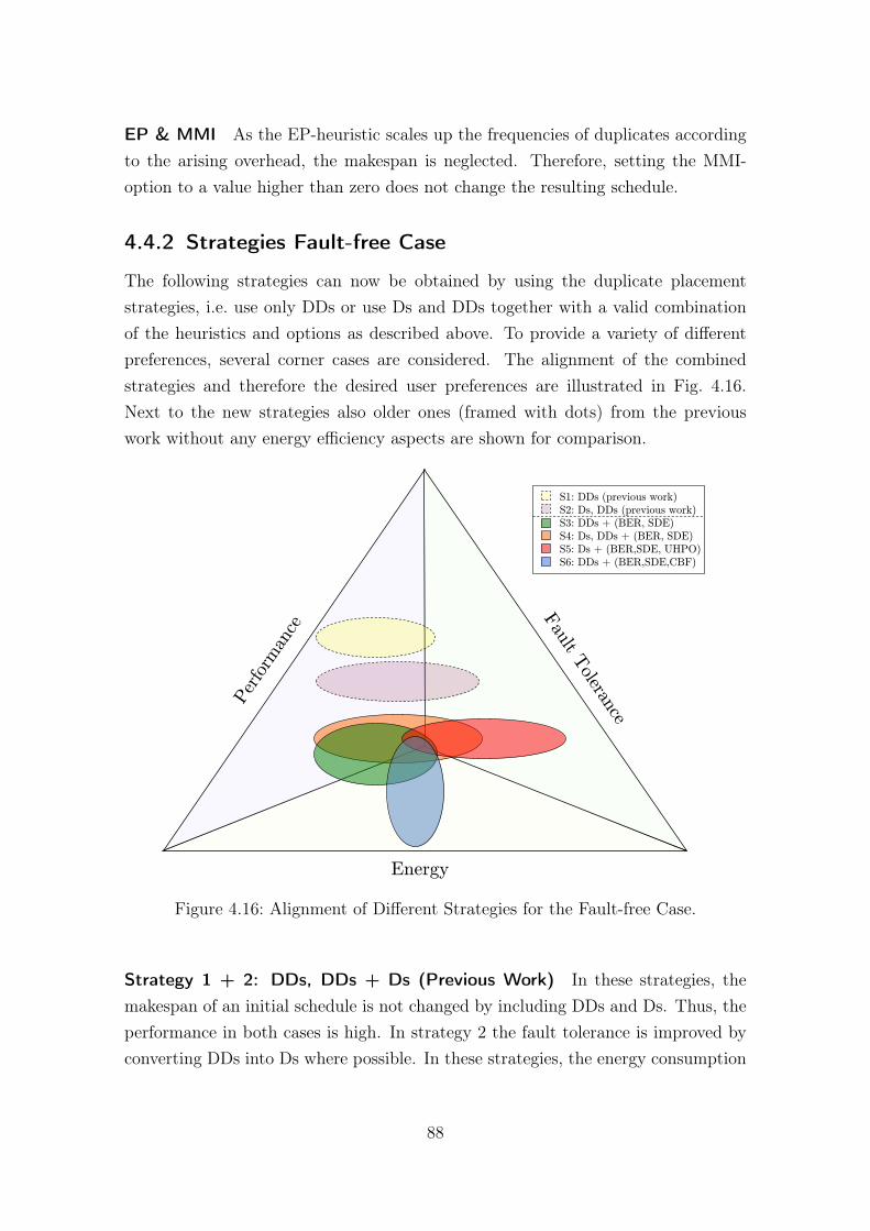
EP & MMI As the EP-heuristic scales up the frequencies of duplicates accordingto the arising overhead, the makespan is neglected. Therefore, setting the MMI-option to a value higher than zero does not change the resulting schedule.

4.4.2 Strategies Fault-free Case

The following strategies can now be obtained by using the duplicate placementstrategies, i.e. use only DDs or use Ds and DDs together with a valid combinationof the heuristics and options as described above. To provide a variety of differentpreferences, several corner cases are considered. The alignment of the combinedstrategies and therefore the desired user preferences are illustrated in Fig. 4.16.Next to the new strategies also older ones (framed with dots) from the previouswork without any energy efficiency aspects are shown for comparison.

S1: DDs (previous work)

S2: Ds, DDs (previous work)

S3: DDs + (BER, SDE)

S4: Ds, DDs + (BER, SDE)

S5: Ds + (BER,SDE, UHPO)

S6: DDs + (BER,SDE,CBF)

Energy

Figure 4.16: Alignment of Different Strategies for the Fault-free Case.

Strategy 1 + 2: DDs, DDs + Ds (Previous Work) In these strategies, themakespan of an initial schedule is not changed by including DDs and Ds. Thus, theperformance in both cases is high. In strategy 2 the fault tolerance is improved byconverting DDs into Ds where possible. In these strategies, the energy consumption

88

is not considered. Both are only related to the performance and the fault tolerance.Therefore, with these strategies the main focus lies on the performance and secondlyon the fault tolerance.

Strategy 3: DDs + (BER, SDE) This strategy is a combination of the firstone, i.e. use only DDs with the BER-heuristic and the SDE-Option. Therefore, theDDs are placed before using any buffers to slowdown tasks by scaling down thefrequencies. The performance and the fault tolerance are equal to strategy 1. Butthe energy consumption is decreased by using the BER-heuristic. Thus, with thisstrategy the user mainly focuses on the performance and secondly on the energyconsumption. The fault tolerance is considered, but should not influence the othercriteria.

Strategy 4: Ds, DDs + (BER, SDE) Instead of using only DDs to improvethe fault tolerance, here Ds are used, too. Thus, the performance is still the mostimportant criterion, but energy is invested to get a better fault tolerance. Therefore,with this strategy the user would like to compensate (partly) the energy spent forthe fault tolerance by slowing down tasks and reducing the energy consumption withthe BER-heuristic.

Strategy 5: Ds + (BER, SDE, UHPO) In strategy 5, the second strategy iscombined with the BER-, UHPO-heuristic and the SDE-Option. The main focuslies on the fault tolerance, i.e. half of the PUs are used for duplicates, the other halffor original tasks. However, the performance is significantly decreased because taskshave to be re-mapped onto fewer PUs and the energy consumption is significantlyincreased, because the whole schedule is executed twice. Only a small benefit canbe gained by using the BER-Option.

Strategy 6: DDs + (BER, SDE, CBF) To achieve a low energy consumption,the base frequency of tasks is changed and only DDs are used for the fault toler-ance. The performance is significantly decreased. Additionally, the BER-heuristic isconsidered, to further reduce the energy consumption. Hence, the main focus of theuser is put on the energy consumption and only a minor part on the other criteria.

89

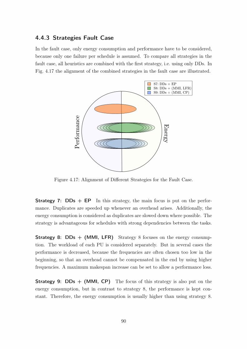
4.4.3 Strategies Fault Case

In the fault case, only energy consumption and performance have to be considered,because only one failure per schedule is assumed. To compare all strategies in thefault case, all heuristics are combined with the first strategy, i.e. using only DDs. InFig. 4.17 the alignment of the combined strategies in the fault case are illustrated.

S7: DDs + EP

S8: DDs + (MMI, LFR)

S9: DDs + (MMI, CP)

Per

form

ance

E

nerg

y

Figure 4.17: Alignment of Different Strategies for the Fault Case.

Strategy 7: DDs + EP In this strategy, the main focus is put on the perfor-mance. Duplicates are speeded up whenever an overhead arises. Additionally, theenergy consumption is considered as duplicates are slowed down where possible. Thestrategy is advantageous for schedules with strong dependencies between the tasks.

Strategy 8: DDs + (MMI, LFR) Strategy 8 focuses on the energy consump-tion. The workload of each PU is considered separately. But in several cases theperformance is decreased, because the frequencies are often chosen too low in thebeginning, so that an overhead cannot be compensated in the end by using higherfrequencies. A maximum makespan increase can be set to allow a performance loss.

Strategy 9: DDs + (MMI, CP) The focus of this strategy is also put on theenergy consumption, but in contrast to strategy 8, the performance is kept con-stant. Therefore, the energy consumption is usually higher than using strategy 8.

90

This strategy is advantageous for schedules with a uniform distribution of the to-tal workload. A maximum makespan increase can be set to improve the energyconsumption.

4.5 Energy-optimal Solutions and Approximations

When the focus is put on the energy, an energy-optimal solution would be preferable.As the scheduling time for optimal solutions is disproportionally high compared tothe energy savings, heuristics like the above explained are often used in practice.However, energy-optimal solutions (calculated at least for small schedules) can beused to rate the quality of the heuristics. Therefore, as demonstrated by Eitschbergerand Keller [56], a mixed integer linear program (ILP) formulation is described asfollows to compute energy optimal solutions in both the fault-free and the fault case.For simplicity, a quadratic power model is assumed, i.e. P (f) = f 2 for a frequency f ,but also other power profiles are possible. Additionally, in case of a failure anotheralternative is to re-schedule the remaining part of the schedule [56] instead of usingthe pre-calculated mapping and ordering. Hence, an approximation and an optimalsolution for the approaches is described for the fault case, i.e. using the existingmapping and using the re-scheduling approach for comparison.

4.5.1 Fault-free Case

To schedule n tasks onto a target system with p PUs and K frequency levels fk,n · p · K binary variables xi,j,k are needed with xi,j,k = 1 if and only if task i isscheduled onto PU j with frequency level k. The energy consumption of a task irunning at frequency level fk is then the product of task runtime ri and the powerconsumption P (fk):

Ei =∑j

∑k

xi,j,k · ri · P (fk). (4.1)

The runtime of a task at frequency level fk depends on the task workload wi andcan be expressed by

ri =∑j

∑k

xi,j,k ·wifk. (4.2)

The total energy consumption of a schedule for a given deadline Dl can then beobtained by summing up the energy consumption of all tasks (assuming that the

91

idle power and therefore the energy for all idle times is neglected for simplicity).Thus, the target function to be minimized is

E =∑i

Ei. (4.3)

The following constraints are used to obtain feasible solutions. Each task mustbe scheduled within the deadline. Hence, the start time si of a task i must be atleast zero and its end time ei = si + ri is not larger than the deadline:

∀i : si ≥ 0 and ei ≤ Dl. (4.4)

Each task must be mapped exactly once in the schedule:

∀i :∑j

∑k

xi,j,k = 1. (4.5)

To indicate whether task i precedes task i′ or not, n2 binary variables yi,i′ are usedwith yi,i′ = 1 if and only if task i precedes task i′ on a common PU. Then task i′

can only start after task i, i.e.

∀i, i′ : si′ ≥ ei − (1− yi,i′) · C, (4.6)

where C is a constant larger than Dl, e.g. C = 2 ·Dl. When both tasks are mappedonto the same PU and i precedes i′, yi,i′ = 1 and the right-hand side of this constraintresults in ei, otherwise the right-hand side is smaller than zero.A task i can not precede itself, thus

∀i : yi,i = 0. (4.7)

Either two tasks i and i′ are succeeding tasks on a common PU so that one ofthem precedes the other one, or they are mapped onto different PUs. However, bothcan not precede each other:

∀i, i′ : yi,i′ + yi′,i ≤ 1. (4.8)

92

Two tasks i and i′ can only be succeeding tasks, when they are mapped onto thesame PU, i.e.

∀i, i′ 6= i, j : yi,i′ + yi′,i ≥ −1 +∑k

(xi,j,k + xi′,j,k). (4.9)

The right-hand side either results in 1, when both tasks are on PU j and thus theright-hand sum is 2, or it results in a value less or equal to zero, i.e. one or bothtasks are mapped onto another PU.

When two tasks i and i′ are mapped onto different PUs, they can not be succeedingtasks, i.e. the variable yi,i′ is then forced to zero:

∀i, i′ 6= i : yi,i′ ≤ 2−∑j,j′ 6=j

∑k

(xi,j,k + xi′,j′,k). (4.10)

To consider dependencies and communication times between tasks, the followingconstraint is necessary: If task i′ is a successor task of task i, i.e. an edge existsbetween both tasks in the task graph, and both are mapped onto different PUs,then the communication time ci,i′ between them must be considered and task i′ canstart after the communication. When the tasks are mapped onto the same PU,task i′ can only start after task i:

∀i, i′ : edge (i, i′) : si′ ≥ ei + (1− yi,i′) · ci,i′ . (4.11)

In this constraint (1− yi,i′) ensures that the communication time is only considered,when both tasks are not mapped onto the same PU, i.e. yi, i′ = 0.

4.5.2 Fault Case

A failure of a PU can occur at any time during the execution of a schedule. To havea small finite number of failure points, only one failure per task is considered. Thelongest delay for broadcasting a failure is when it occurs at the beginning of a task,because the remaining PUs are informed about the failure by the missing commitmessage. In the fault case, optimal solutions for the already existing mapping canbe calculated for each failure point. Then, the optimal schedules can be used toevaluate the fault case heuristics, as they use the already existing tasks (originals andduplicates) and only change the frequencies and the start times of tasks dynamically,but not the ordering or the mapping. As a general placement of duplicates cannot

93

be optimal for each fault case, they have to be placed in different ways dependingon the failure position to get an optimal solution. Therefore, another approach isto re-schedule the tasks in case of a failure onto the remaining p − 1 PUs, insteadof running on p PUs. This can be done statically prior to execution for each failureposition, i.e. for each original task that fails. Then, the execution time of a scheduleis not influenced by the scheduling time and a corresponding runtime system canchoose the optimal schedule according to the failure point.

Existing Mapping To find an optimal solution for the existing mapping, only thedependencies and communication times must be considered next to end times oftasks. Therefore, an explicit declaration of PUs is unnecessary in this case. Toformulate an ILP the energy consumption for a task i can be expressed by:

Ei = P (f) · wif

(4.12)

where P (f) is the power consumption at frequency f and wi is the workload oftask i. Now, an approximation close to an optimal solution can be obtained byusing n · K binary variables xi,k for n tasks and K frequency levels fk each withxi,k = 1 if and only if task i is executed with a frequency level fk. A frequency rangebetween 0.1 and 2 with a step size of 0.05 is used. The energy consumption for aschedule can then be expressed by:

E =∑i

∑k

xi,k · wi ·P (f)

fk. (4.13)

The end time ei of an ending task i must be less than or equal to the deadline:

∀i = ending task : ei ≤ Dl. (4.14)

The end time ei of an entry task i is at least the runtime of the task, i.e.

∀i = entry task : ei ≥∑k

xi,k ·wifk. (4.15)

Only one frequency level can be used for each task, thus

∀i :∑k

xi,k = 1. (4.16)

94

A task i can only be started after all predecessor tasks i′. If a predecessor i′ ismapped onto another PU, the communication time cti′,i can be directly includedas a constant, otherwise it is set to zero. Then, the end time ei of a task can beexpressed by

∀i : ∀i′ ∈ pred(i) : ei ≥∑k

xi,k ·wifk

+ cti′,i + ei′ . (4.17)

Note, that this constraint is set for every predecessor task explicitly to fix the map-ping and ordering of the tasks, e.g. if a task has three predecessors, this constraintis included three times.

As only the time between the failure point and the deadline is considered in theILP, all tasks that start before and finish after the failure are cut at the failure timeand the remaining part after the failure is included as workload. For these tasks,the frequency level fk is fixed by setting xi,k = 1, because only one frequency pertask is allowed.

Re-scheduling An optimal solution for the re-scheduling in case of a failure can beachieved by modifying the above explained mixed ILP for the fault-free case. For alltasks that start before the end of the failing task, the mapping, frequencies and starttimes and thus the x- and s-variables in the mixed ILP are fixed. As the duplicateof the failing task can only be started after its corresponding original task, the starttime of the duplicate is bound by the end time of the failed original task. The faultyPU cannot be used after the failure and all remaining tasks cannot be mapped ontothe faulty PU. This is considered by forcing the corresponding x-variables to zero.The MMI-Option, i.e. when a prolongation of a schedule is allowed, can be includedby changing the deadline according to the given percentage value.

95

96

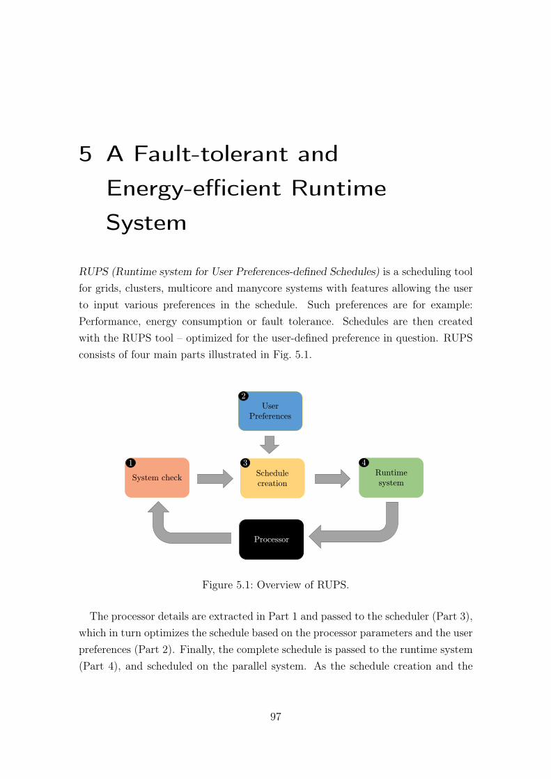
5 A Fault-tolerant andEnergy-efficient RuntimeSystem

RUPS (Runtime system for User Preferences-defined Schedules) is a scheduling toolfor grids, clusters, multicore and manycore systems with features allowing the userto input various preferences in the schedule. Such preferences are for example:Performance, energy consumption or fault tolerance. Schedules are then createdwith the RUPS tool – optimized for the user-defined preference in question. RUPSconsists of four main parts illustrated in Fig. 5.1.

System check Schedule

creation

Runtime

system

Processor

1 3 4

User

Preferences

2

Figure 5.1: Overview of RUPS.

The processor details are extracted in Part 1 and passed to the scheduler (Part 3),which in turn optimizes the schedule based on the processor parameters and the userpreferences (Part 2). Finally, the complete schedule is passed to the runtime system(Part 4), and scheduled on the parallel system. As the schedule creation and the

97

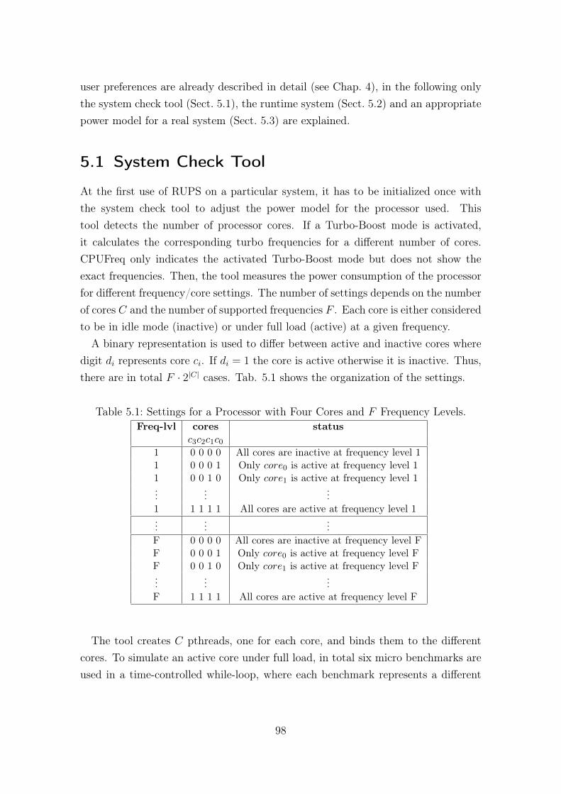
user preferences are already described in detail (see Chap. 4), in the following onlythe system check tool (Sect. 5.1), the runtime system (Sect. 5.2) and an appropriatepower model for a real system (Sect. 5.3) are explained.

5.1 System Check Tool

At the first use of RUPS on a particular system, it has to be initialized once withthe system check tool to adjust the power model for the processor used. Thistool detects the number of processor cores. If a Turbo-Boost mode is activated,it calculates the corresponding turbo frequencies for a different number of cores.CPUFreq only indicates the activated Turbo-Boost mode but does not show theexact frequencies. Then, the tool measures the power consumption of the processorfor different frequency/core settings. The number of settings depends on the numberof cores C and the number of supported frequencies F . Each core is either consideredto be in idle mode (inactive) or under full load (active) at a given frequency.

A binary representation is used to differ between active and inactive cores wheredigit di represents core ci. If di = 1 the core is active otherwise it is inactive. Thus,there are in total F · 2|C| cases. Tab. 5.1 shows the organization of the settings.

Table 5.1: Settings for a Processor with Four Cores and F Frequency Levels.Freq-lvl cores status

c3c2c1c01 0 0 0 0 All cores are inactive at frequency level 11 0 0 0 1 Only core0 is active at frequency level 11 0 0 1 0 Only core1 is active at frequency level 1...

......

1 1 1 1 1 All cores are active at frequency level 1...

......

F 0 0 0 0 All cores are inactive at frequency level FF 0 0 0 1 Only core0 is active at frequency level FF 0 0 1 0 Only core1 is active at frequency level F...

......

F 1 1 1 1 All cores are active at frequency level F

The tool creates C pthreads, one for each core, and binds them to the differentcores. To simulate an active core under full load, in total six micro benchmarks areused in a time-controlled while-loop, where each benchmark represents a different

98

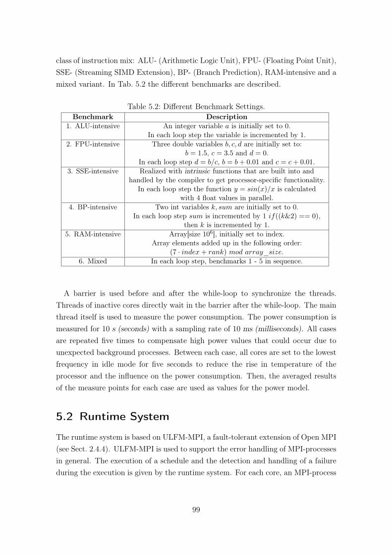
class of instruction mix: ALU- (Arithmetic Logic Unit), FPU- (Floating Point Unit),SSE- (Streaming SIMD Extension), BP- (Branch Prediction), RAM-intensive and amixed variant. In Tab. 5.2 the different benchmarks are described.

Table 5.2: Different Benchmark Settings.Benchmark Description

1. ALU-intensive An integer variable a is initially set to 0.In each loop step the variable is incremented by 1.

2. FPU-intensive Three double variables b, c, d are initially set to:b = 1.5, c = 3.5 and d = 0.

In each loop step d = b/c, b = b+ 0.01 and c = c+ 0.01.3. SSE-intensive Realized with intrinsic functions that are built into and

handled by the compiler to get processor-specific functionality.In each loop step the function y = sin(x)/x is calculated

with 4 float values in parallel.4. BP-intensive Two int variables k, sum are initially set to 0.

In each loop step sum is incremented by 1 if((k&2) == 0),then k is incremented by 1.

5. RAM-intensive Array[size 106], initially set to index.Array elements added up in the following order:

(7 · index+ rank) mod array_size.6. Mixed In each loop step, benchmarks 1 - 5 in sequence.

A barrier is used before and after the while-loop to synchronize the threads.Threads of inactive cores directly wait in the barrier after the while-loop. The mainthread itself is used to measure the power consumption. The power consumption ismeasured for 10 s (seconds) with a sampling rate of 10 ms (milliseconds). All casesare repeated five times to compensate high power values that could occur due tounexpected background processes. Between each case, all cores are set to the lowestfrequency in idle mode for five seconds to reduce the rise in temperature of theprocessor and the influence on the power consumption. Then, the averaged resultsof the measure points for each case are used as values for the power model.

5.2 Runtime System

The runtime system is based on ULFM-MPI, a fault-tolerant extension of Open MPI(see Sect. 2.4.4). ULFM-MPI is used to support the error handling of MPI-processesin general. The execution of a schedule and the detection and handling of a failureduring the execution is given by the runtime system. For each core, an MPI-process

99

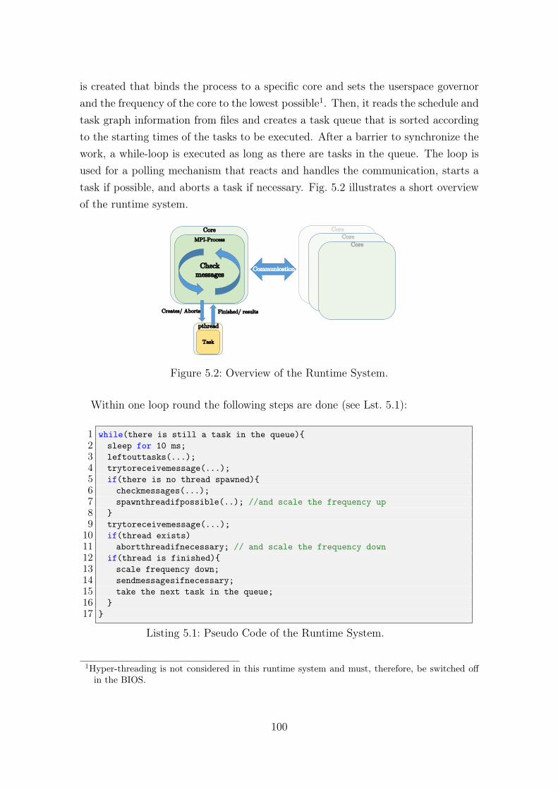
is created that binds the process to a specific core and sets the userspace governorand the frequency of the core to the lowest possible1. Then, it reads the schedule andtask graph information from files and creates a task queue that is sorted accordingto the starting times of the tasks to be executed. After a barrier to synchronize thework, a while-loop is executed as long as there are tasks in the queue. The loop isused for a polling mechanism that reacts and handles the communication, starts atask if possible, and aborts a task if necessary. Fig. 5.2 illustrates a short overviewof the runtime system.

Task

pthread

MPI-Process

Check

messages

Core

Core

Core

Core

Communication

Creates/ Aborts Finished/ results

Figure 5.2: Overview of the Runtime System.

Within one loop round the following steps are done (see Lst. 5.1):

1 while(there is still a task in the queue){2 sleep for 10 ms;3 leftouttasks(...);4 trytoreceivemessage(...);5 if(there is no thread spawned){6 checkmessages(...);7 spawnthreadifpossible(..); //and scale the frequency up8 }9 trytoreceivemessage(...);10 if(thread exists)11 abortthreadifnecessary; // and scale the frequency down12 if(thread is finished){13 scale frequency down;14 sendmessagesifnecessary;15 take the next task in the queue;16 }17 }

Listing 5.1: Pseudo Code of the Runtime System.

1Hyper-threading is not considered in this runtime system and must, therefore, be switched offin the BIOS.

100

• The core sleeps for 10 ms to minimize the polling overhead (line 2).

• It is checked whether a task can be left out, e.g. a duplicate that could startnext but that already received a commit message from the original task. Inthis case, it does not have to be executed (line 3).

• A message is tried to receive, that can mainly include either some resultsof another task or a commit message for a duplicate. In this version of theruntime system, just the message header is sent as results. The message headerincludes, next to others, the information about the task for which the messageis destined, what kind of data will be sent, how much memory is needed for thedata, the start time of the sending operation and the time that is needed for thetransfer. The latter two are used to simulate the transfer. The communicationis done on the sender side with a blocking MPI_send operation, on the receiverside with an unblocking MPI_iProbe to check if there is a message for the core.If so, a blocking MPI_recv operation is used to receive the message. Thus, thesender is blocked as long as the message is not sent, the receiver is blockedonly if there is a message for it. Otherwise, it can continue with the remainingpart of the while-loop (line 4).

• If no other task is running and if all results of the predecessor tasks are al-ready received, the frequency is scaled up and the task is started by spawning athread. To simulate an expensive calculation one of the six micro benchmarksfrom Sect. 5.1 is used for the computation time of the task. The task executionis separated from the communication process by a thread (see Fig. 5.2) so thatthe structure of a task is independent of the communication. Especially theruntime system lacks information about the task itself and about the functionsthat are done within the task. Thus, it could be impossible to interrupt thetask execution at some points for trying to receive some messages. Further-more, one thread is used for each task and not one thread for all tasks. Thetasks on one core are executed one by one so that at each time just one threador task is running. Another possibility would be to spawn only one thread forall task executions, but then a task cannot be aborted if necessary becausesome polling mechanism would be needed again that cannot be included inthe task because of the missing knowledge of the task structure. Two flags areused to indicate whether a task is running or not and if a task has just finished(lines 5 - 8).

101

• After this the process once again tries to receive a message. This is necessaryto avoid deadlocks that could appear if two cores try to send a message toeach other (line 9).

• If a task is already running and if it is a duplicate, check if the duplicate hasto be aborted because of a receiving commit message from the original task.If a duplicate should be aborted, the corresponding thread is canceled and thefrequency is scaled down to the lowest possible (lines 10 - 11).

• Otherwise, it is checked if the thread has finished, the frequency is scaleddown to the lowest possible and the results are sent to the successor tasks ifnecessary (lines 12 - 17).

After the while loop a second barrier is used to indicate that the schedule execu-tion is finished. To implement the runtime system in an energy-efficient way, it isimportant that some MPI-operations like a blocking receive or a barrier use a busywaiting mechanism. If an MPI-process is running in those operations for a longertime, the corresponding core wastes energy because it is under full load for this time.Thus, those operations should be used carefully. Therefore, in this runtime systeman MPI_iProbe is used before every blocking receive. Also the second barrier afterthe while loop is realized in this way.

The runtime system supports a testing mode, where one additional MPI-processis started next to the above sequence to measure the energy consumption with thehelp of the Intel RAPL feature (see Sect. 2.5.4). The measurement process measuresthe energy for the time of the whole while loop, because this is the time needed forthe execution of the total schedule. The sample rate of the measurement is 10 ms.This process is not bound to a specific core like the other processes, so it can run onany core. There are some performance and energy overheads that occur by runningthe testing mode with the further process. But the influence can be neglected fortwo reasons: The energy overhead is included in the measurements of the systemcheck that are done by a master thread. Thus, the energy values for the power modelconsider this overhead. And the performance overhead is less than one percent of aprocessor core. Therefore, the influence on the task execution is low.

Until now, the runtime system is described in general but not, how a failure of aPU (here a PU represents a processor core) can be handled. A failure is simulatedby exiting an MPI-process just before the corresponding task is started, i.e. in thefunction spawnthreadifpossible(). The other processes are informed about the

102

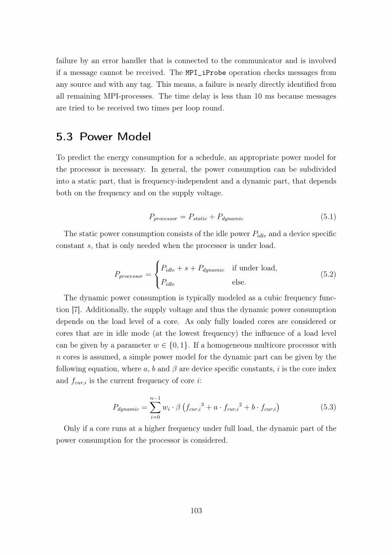
failure by an error handler that is connected to the communicator and is involvedif a message cannot be received. The MPI_iProbe operation checks messages fromany source and with any tag. This means, a failure is nearly directly identified fromall remaining MPI-processes. The time delay is less than 10 ms because messagesare tried to be received two times per loop round.

5.3 Power Model

To predict the energy consumption for a schedule, an appropriate power model forthe processor is necessary. In general, the power consumption can be subdividedinto a static part, that is frequency-independent and a dynamic part, that dependsboth on the frequency and on the supply voltage.

Pprocessor = Pstatic + Pdynamic (5.1)

The static power consumption consists of the idle power Pidle and a device specificconstant s, that is only needed when the processor is under load.

Pprocessor =

Pidle + s+ Pdynamic if under load,

Pidle else.(5.2)

The dynamic power consumption is typically modeled as a cubic frequency func-tion [7]. Additionally, the supply voltage and thus the dynamic power consumptiondepends on the load level of a core. As only fully loaded cores are considered orcores that are in idle mode (at the lowest frequency) the influence of a load levelcan be given by a parameter w ∈ {0, 1}. If a homogeneous multicore processor withn cores is assumed, a simple power model for the dynamic part can be given by thefollowing equation, where a, b and β are device specific constants, i is the core indexand fcur,i is the current frequency of core i:

Pdynamic =n−1∑i=0

wi · β(fcur,i

3 + a · fcur,i2 + b · fcur,i)

(5.3)

Only if a core runs at a higher frequency under full load, the dynamic part of thepower consumption for the processor is considered.

103

104

6 Experiments

6.1 Test Environment

6.1.1 Test Sets

To evaluate the heuristics and strategies presented in Chap. 4, a benchmark suite of36,000 synthetic task graphs and schedules for small cases with up to 24 tasks and36,000 task graphs for large cases with up to 250 tasks is used [84]. The task graphsare subdivided into several groups according to their properties. As the organizationof the benchmark suite for small and large cases differs in the intervals of task countonly, the structure is described for both together. One property is the size of thetarget system that is considered by the number of PUs. In total 5 groups exist with2, 4, 8, 16 and 32 PUs and with 7,200 task graphs each. Every group is categorizedby the number of tasks into 3 subgroups: 7 - 12, 13 - 18 and 19 - 24 tasks for thesmall cases and 25 - 99, 100 - 174 and 175 - 250 tasks for the large cases. In eachinterval 2,400 task graphs exist that are further subdivided by the edge density inlow, average, high and random. Each of these groups contains 600 task graphs thatare further differentiated by the edge length into short, average, long and random.The remaining 150 task graphs per group are finally subdivided by the edge andnode weights into 5 groups with high node/high edge, high node/low edge, lownode/high edge, low node/low edge and random node/random edge weights. In 4 ofthese groups are 25 task graphs each. The group of random node and edge weightsconsists of 50 task graphs. In general, the benchmark suite is organized as a flatfile database, where the structure is given by the directory tree [84]. The principleorganization is shown in Fig. 6.1.

Based on the task graphs for small cases, two schedule sets with performanceoptimized schedules are used that were generated by Hönig [84]. Both schedule setscomprise nearly 34,000 schedules each, because for some task graphs no optimizedsolution was found. The first schedule set, called TB-Optimal (Test Benchmark),comprises performance optimal schedules. These schedules were generated with a

105

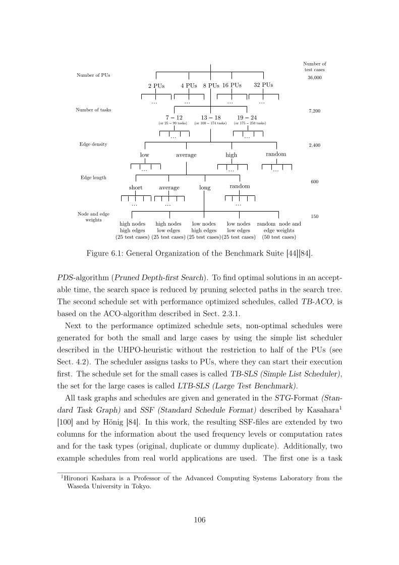
(or 25 – 99 tasks) (or 100 – 174 tasks) (or 175 – 250 tasks)

2 PUs 4 PUs 8 PUs 16 PUs 32 PUs

… … … …

7 – 12 13 – 18 19 – 24

… …

low average high random

… … …

short average long random

… … …

high nodes

high edges

(25 test cases)

high nodes

low edges

(25 test cases)

low nodes

high edges

(25 test cases)

random node and

edge weights

(50 test cases)

low nodes

low edges

(25 test cases)

Number of PUs

Number of tasks

Edge density

Edge length

Node and edge

weights

Number of

test cases

150

7,200

2,400

600

36,000

Figure 6.1: General Organization of the Benchmark Suite [44][84].

PDS-algorithm (Pruned Depth-first Search). To find optimal solutions in an accept-able time, the search space is reduced by pruning selected paths in the search tree.The second schedule set with performance optimized schedules, called TB-ACO, isbased on the ACO-algorithm described in Sect. 2.3.1.

Next to the performance optimized schedule sets, non-optimal schedules weregenerated for both the small and large cases by using the simple list schedulerdescribed in the UHPO-heuristic without the restriction to half of the PUs (seeSect. 4.2). The scheduler assigns tasks to PUs, where they can start their executionfirst. The schedule set for the small cases is called TB-SLS (Simple List Scheduler),the set for the large cases is called LTB-SLS (Large Test Benchmark).All task graphs and schedules are given and generated in the STG-Format (Stan-

dard Task Graph) and SSF (Standard Schedule Format) described by Kasahara1

[100] and by Hönig [84]. In this work, the resulting SSF-files are extended by twocolumns for the information about the used frequency levels or computation ratesand for the task types (original, duplicate or dummy duplicate). Additionally, twoexample schedules from real world applications are used. The first one is a task

1Hironori Kashara is a Professor of the Advanced Computing Systems Laboratory from theWaseda University in Tokyo.

106

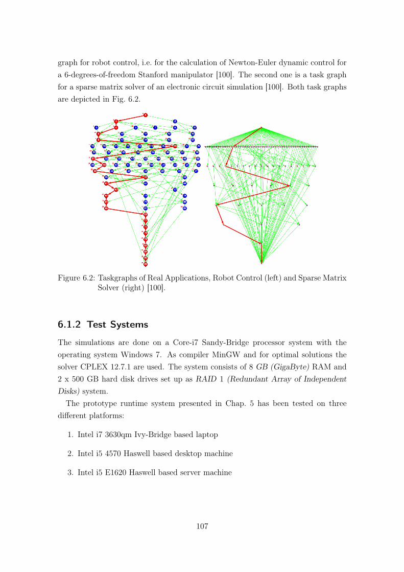
graph for robot control, i.e. for the calculation of Newton-Euler dynamic control fora 6-degrees-of-freedom Stanford manipulator [100]. The second one is a task graphfor a sparse matrix solver of an electronic circuit simulation [100]. Both task graphsare depicted in Fig. 6.2.

Figure 6.2: Taskgraphs of Real Applications, Robot Control (left) and Sparse MatrixSolver (right) [100].

6.1.2 Test Systems

The simulations are done on a Core-i7 Sandy-Bridge processor system with theoperating system Windows 7. As compiler MinGW and for optimal solutions thesolver CPLEX 12.7.1 are used. The system consists of 8 GB (GigaByte) RAM and2 x 500 GB hard disk drives set up as RAID 1 (Redundant Array of IndependentDisks) system.The prototype runtime system presented in Chap. 5 has been tested on three

different platforms:

1. Intel i7 3630qm Ivy-Bridge based laptop

2. Intel i5 4570 Haswell based desktop machine

3. Intel i5 E1620 Haswell based server machine

107

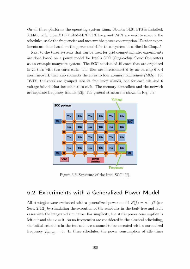
On all three platforms the operating system Linux Ubuntu 14.04 LTS is installed.Additionally, OpenMPI/ULFM-MPI, CPUFreq, and PAPI are used to execute theschedules, scale the frequencies and measure the power consumption. Further exper-iments are done based on the power model for these systems described in Chap. 5.

Next to the three systems that can be used for grid computing, also experimentsare done based on a power model for Intel’s SCC (Single-chip Cloud Computer)as an example manycore system. The SCC consists of 48 cores that are organizedin 24 tiles with two cores each. The tiles are interconnected by an on-chip 6 × 4

mesh network that also connects the cores to four memory controllers (MCs). ForDVFS, the cores are grouped into 24 frequency islands, one for each tile and 6voltage islands that include 4 tiles each. The memory controllers and the networkare separate frequency islands [92]. The general structure is shown in Fig. 6.3.

Tile

Tile

Tile

Tile

Tile

Tile

Tile

Tile

Tile

Tile

Tile

Tile

MC MC

MC MC

VRC System

Interface

SCC package

R

R

R

R

R

R

R

R

R

R

R

R

Tile

Tile

Tile

Tile

Tile

Tile

Tile

Tile

Tile

Tile

Tile

Tile

R

R

R

R

R

R

R

R

R

R

R

R

Voltage

Frequency

Figure 6.3: Structure of the Intel SCC [92].

6.2 Experiments with a Generalized Power Model

All strategies were evaluated with a generalized power model P (f) = c + f 3 (seeSect. 2.5.2) by simulating the execution of the schedules in the fault-free and faultcases with the integrated simulator. For simplicity, the static power consumption isleft out and thus c = 0. As no frequencies are considered in the classical scheduling,the initial schedules in the test sets are assumed to be executed with a normalizedfrequency fnormal = 1. In these schedules, the power consumption of idle times

108

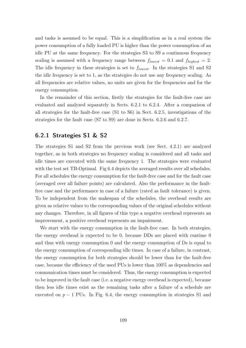
and tasks is assumed to be equal. This is a simplification as in a real system thepower consumption of a fully loaded PU is higher than the power consumption of anidle PU at the same frequency. For the strategies S3 to S9 a continuous frequencyscaling is assumed with a frequency range between flowest = 0.1 and fhighest = 2.The idle frequency in these strategies is set to flowest. In the strategies S1 and S2the idle frequency is set to 1, as the strategies do not use any frequency scaling. Asall frequencies are relative values, no units are given for the frequencies and for theenergy consumption.

In the remainder of this section, firstly the strategies for the fault-free case areevaluated and analyzed separately in Sects. 6.2.1 to 6.2.4. After a comparison ofall strategies for the fault-free case (S1 to S6) in Sect. 6.2.5, investigations of thestrategies for the fault case (S7 to S9) are done in Sects. 6.2.6 and 6.2.7.

6.2.1 Strategies S1 & S2

The strategies S1 and S2 from the previous work (see Sect. 4.2.1) are analyzedtogether, as in both strategies no frequency scaling is considered and all tasks andidle times are executed with the same frequency 1. The strategies were evaluatedwith the test set TB-Optimal. Fig 6.4 depicts the averaged results over all schedules.For all schedules the energy consumption for the fault-free case and for the fault case(averaged over all failure points) are calculated. Also the performance in the fault-free case and the performance in case of a failure (rated as fault tolerance) is given.To be independent from the makespan of the schedules, the overhead results aregiven as relative values to the corresponding values of the original schedules withoutany changes. Therefore, in all figures of this type a negative overhead represents animprovement, a positive overhead represents an impairment.

We start with the energy consumption in the fault-free case. In both strategies,the energy overhead is expected to be 0, because DDs are placed with runtime 0and thus with energy consumption 0 and the energy consumption of Ds is equal tothe energy consumption of corresponding idle times. In case of a failure, in contrast,the energy consumption for both strategies should be lower than for the fault-freecase, because the efficiency of the used PUs is lower than 100% as dependencies andcommunication times must be considered. Thus, the energy consumption is expectedto be improved in the fault case (i.e. a negative energy overhead is expected), becausethen less idle times exist as the remaining tasks after a failure of a schedule areexecuted on p − 1 PUs. In Fig. 6.4, the energy consumption in strategies S1 and

109

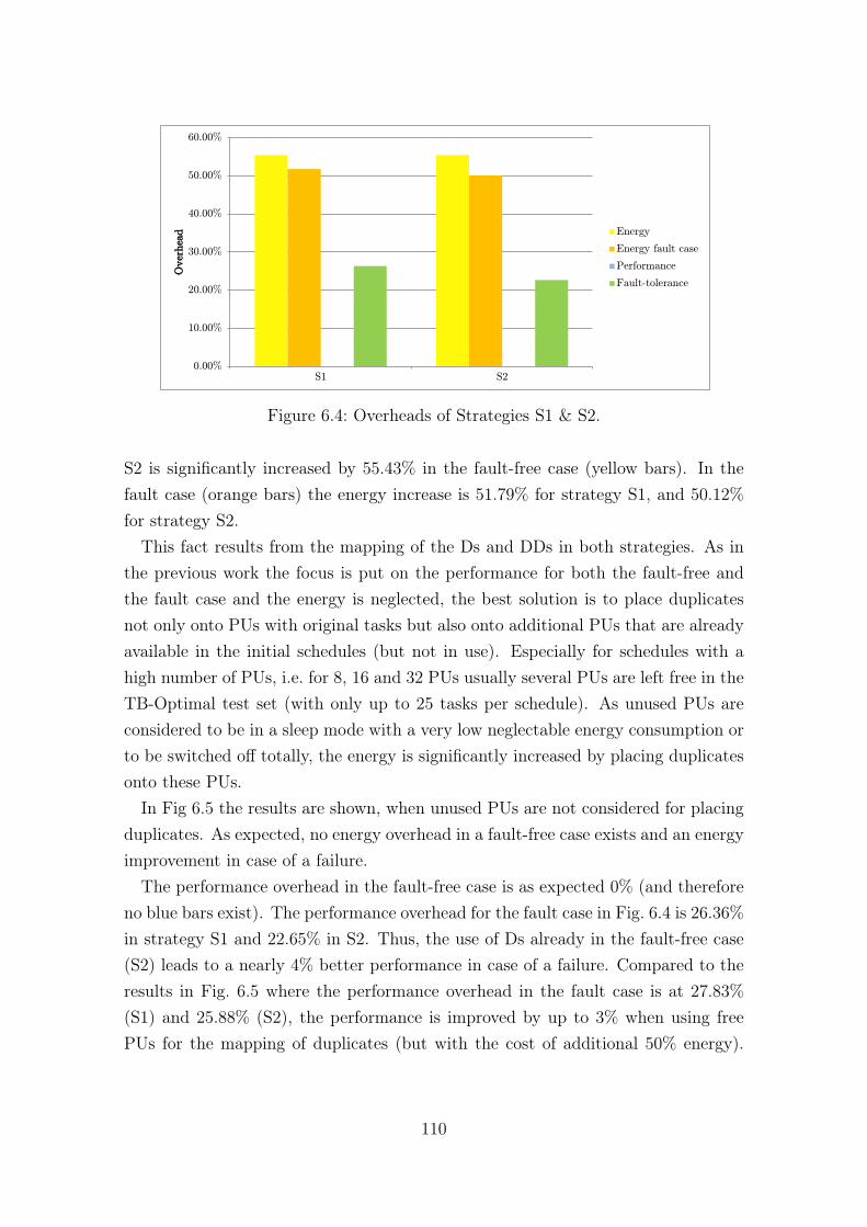
0.00%

10.00%

20.00%

30.00%

40.00%

50.00%

60.00%

S1 S2

Over

hea

d

Energy

Energy fault case

Performance

Fault-tolerance

Figure 6.4: Overheads of Strategies S1 & S2.

S2 is significantly increased by 55.43% in the fault-free case (yellow bars). In thefault case (orange bars) the energy increase is 51.79% for strategy S1, and 50.12%for strategy S2.

This fact results from the mapping of the Ds and DDs in both strategies. As inthe previous work the focus is put on the performance for both the fault-free andthe fault case and the energy is neglected, the best solution is to place duplicatesnot only onto PUs with original tasks but also onto additional PUs that are alreadyavailable in the initial schedules (but not in use). Especially for schedules with ahigh number of PUs, i.e. for 8, 16 and 32 PUs usually several PUs are left free in theTB-Optimal test set (with only up to 25 tasks per schedule). As unused PUs areconsidered to be in a sleep mode with a very low neglectable energy consumption orto be switched off totally, the energy is significantly increased by placing duplicatesonto these PUs.

In Fig 6.5 the results are shown, when unused PUs are not considered for placingduplicates. As expected, no energy overhead in a fault-free case exists and an energyimprovement in case of a failure.

The performance overhead in the fault-free case is as expected 0% (and thereforeno blue bars exist). The performance overhead for the fault case in Fig. 6.4 is 26.36%in strategy S1 and 22.65% in S2. Thus, the use of Ds already in the fault-free case(S2) leads to a nearly 4% better performance in case of a failure. Compared to theresults in Fig. 6.5 where the performance overhead in the fault case is at 27.83%(S1) and 25.88% (S2), the performance is improved by up to 3% when using freePUs for the mapping of duplicates (but with the cost of additional 50% energy).

110

-20.00%

-10.00%

0.00%

10.00%

20.00%

30.00%

40.00%

50.00%

60.00%

S1 S2

Over

hea

d Energy

Energy fault case

Performance

Fault-tolerance

Figure 6.5: Overheads of Strategies S1 & S2 without Using Free PUs.

Therefore, with the assumptions made in the beginning, duplicates should better beplaced onto PUs that were already in use in the initial schedules when no frequencyscaling is possible.

6.2.2 Strategies S3 & S4

The strategies S3 and S4 are extended versions of the strategies S1 and S2 whereenergy efficiency is included by the BER-heuristic (see Sect. 4.4). Additionally, theidle frequency that is used for the gaps within the schedules is set to the lowestpossible frequency flowest. In Fig. 6.6 the results of strategies S3 and S4 for theTB-Optimal test set are shown.

In strategy S3, the energy consumption can be improved by around 40% (40.74%in the fault-free case and 39.52% in the fault case) compared to the original schedules.Since the energy consumption for idle times is very low compared to the energyconsumption of tasks2, the idle times have only a small influence on the total energyconsumption of a schedule. Therefore, the effects on the energy are also negligibleby the use of free processors for the placement of duplicates in the fault-free case.In contrast, the slightly higher energy consumption in case of a failure compared tothe fault-free case results from a non-optimal placement of duplicates that leads tomore and longer gaps after the failure.

2Now the idle frequency is set to 0.1.

111

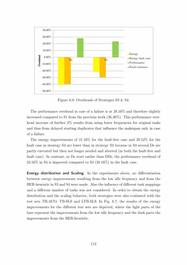
-50.00%

-40.00%

-30.00%

-20.00%

-10.00%

0.00%

10.00%

20.00%

30.00%

40.00%

S3 S4

Over

hea

d Energy

Energy fault case

Performance

Fault-tolerance

Figure 6.6: Overheads of Strategies S3 & S4.

The performance overhead in case of a failure is at 28.16% and therefore slightlyincreased compared to S1 from the previous work (26.36%). This performance over-head increase of further 2% results from using lower frequencies for original tasksand thus from delayed starting duplicates that influence the makespan only in caseof a failure.

The energy improvements of 21.16% for the fault-free case and 29.52% for thefault case in strategy S4 are lower than in strategy S3 because in S4 several Ds arepartly executed but then not longer needed and aborted (in both the fault-free andfault case). In contrast, as Ds start earlier than DDs, the performance overhead of23.56% in S4 is improved compared to S3 (28.16%) in the fault case.

Energy distribution and Scaling In the experiments above, no differentiationbetween energy improvements resulting from the low idle frequency and from theBER-heuristic in S3 and S4 were made. Also the influence of different task mappingsand a different number of tasks was not considered. In order to obtain the energydistribution and the scaling behavior, both strategies were also evaluated with thetest sets TB-ACO, TB-SLS and LTB-SLS. In Fig. 6.7, the results of the energyimprovements for the different test sets are depicted, where the light parts of thebars represent the improvements from the low idle frequency and the dark parts theimprovements from the BER-heuristic.

112

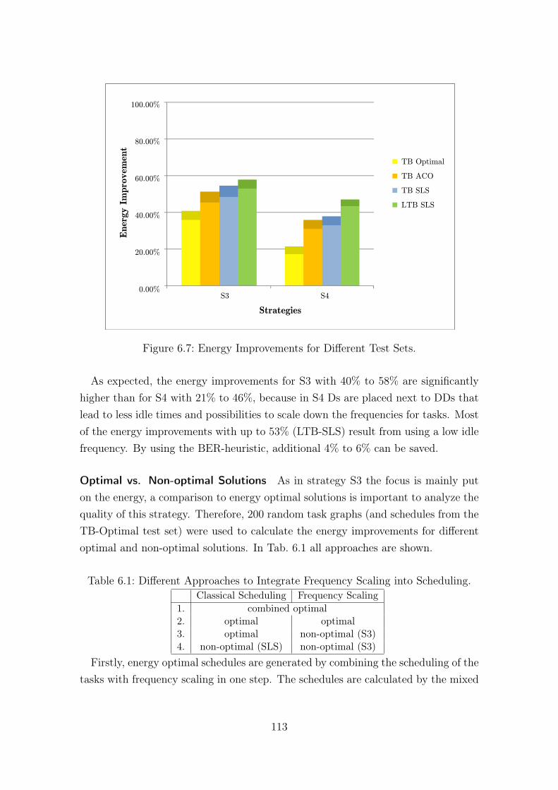
100.00%

80.00%

60.00%

40.00%

20.00%

0.00%

Energ

y I

mpro

vem

ent

S3 S4

Strategies

TB Optimal

TB ACO

TB SLS

LTB SLS

Figure 6.7: Energy Improvements for Different Test Sets.

As expected, the energy improvements for S3 with 40% to 58% are significantlyhigher than for S4 with 21% to 46%, because in S4 Ds are placed next to DDs thatlead to less idle times and possibilities to scale down the frequencies for tasks. Mostof the energy improvements with up to 53% (LTB-SLS) result from using a low idlefrequency. By using the BER-heuristic, additional 4% to 6% can be saved.

Optimal vs. Non-optimal Solutions As in strategy S3 the focus is mainly puton the energy, a comparison to energy optimal solutions is important to analyze thequality of this strategy. Therefore, 200 random task graphs (and schedules from theTB-Optimal test set) were used to calculate the energy improvements for differentoptimal and non-optimal solutions. In Tab. 6.1 all approaches are shown.

Table 6.1: Different Approaches to Integrate Frequency Scaling into Scheduling.Classical Scheduling Frequency Scaling

1. combined optimal2. optimal optimal3. optimal non-optimal (S3)4. non-optimal (SLS) non-optimal (S3)

Firstly, energy optimal schedules are generated by combining the scheduling of thetasks with frequency scaling in one step. The schedules are calculated by the mixed

113

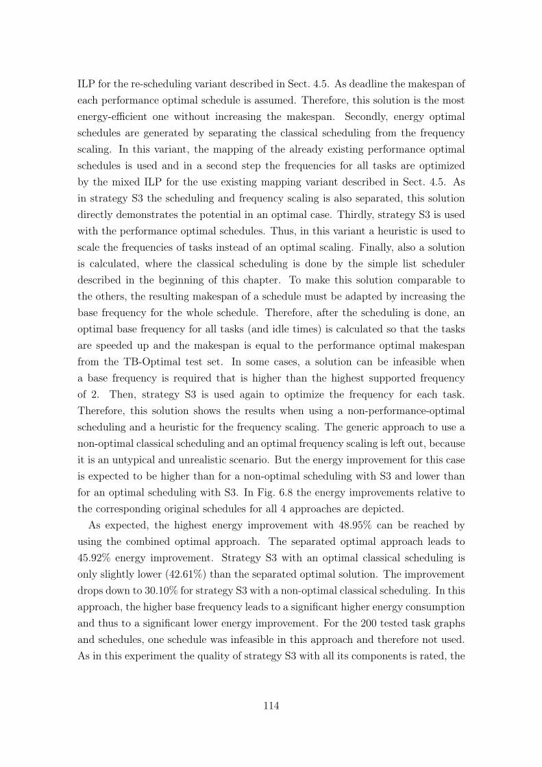
ILP for the re-scheduling variant described in Sect. 4.5. As deadline the makespan ofeach performance optimal schedule is assumed. Therefore, this solution is the mostenergy-efficient one without increasing the makespan. Secondly, energy optimalschedules are generated by separating the classical scheduling from the frequencyscaling. In this variant, the mapping of the already existing performance optimalschedules is used and in a second step the frequencies for all tasks are optimizedby the mixed ILP for the use existing mapping variant described in Sect. 4.5. Asin strategy S3 the scheduling and frequency scaling is also separated, this solutiondirectly demonstrates the potential in an optimal case. Thirdly, strategy S3 is usedwith the performance optimal schedules. Thus, in this variant a heuristic is used toscale the frequencies of tasks instead of an optimal scaling. Finally, also a solutionis calculated, where the classical scheduling is done by the simple list schedulerdescribed in the beginning of this chapter. To make this solution comparable tothe others, the resulting makespan of a schedule must be adapted by increasing thebase frequency for the whole schedule. Therefore, after the scheduling is done, anoptimal base frequency for all tasks (and idle times) is calculated so that the tasksare speeded up and the makespan is equal to the performance optimal makespanfrom the TB-Optimal test set. In some cases, a solution can be infeasible whena base frequency is required that is higher than the highest supported frequencyof 2. Then, strategy S3 is used again to optimize the frequency for each task.Therefore, this solution shows the results when using a non-performance-optimalscheduling and a heuristic for the frequency scaling. The generic approach to use anon-optimal classical scheduling and an optimal frequency scaling is left out, becauseit is an untypical and unrealistic scenario. But the energy improvement for this caseis expected to be higher than for a non-optimal scheduling with S3 and lower thanfor an optimal scheduling with S3. In Fig. 6.8 the energy improvements relative tothe corresponding original schedules for all 4 approaches are depicted.

As expected, the highest energy improvement with 48.95% can be reached byusing the combined optimal approach. The separated optimal approach leads to45.92% energy improvement. Strategy S3 with an optimal classical scheduling isonly slightly lower (42.61%) than the separated optimal solution. The improvementdrops down to 30.10% for strategy S3 with a non-optimal classical scheduling. In thisapproach, the higher base frequency leads to a significant higher energy consumptionand thus to a significant lower energy improvement. For the 200 tested task graphsand schedules, one schedule was infeasible in this approach and therefore not used.As in this experiment the quality of strategy S3 with all its components is rated, the

114

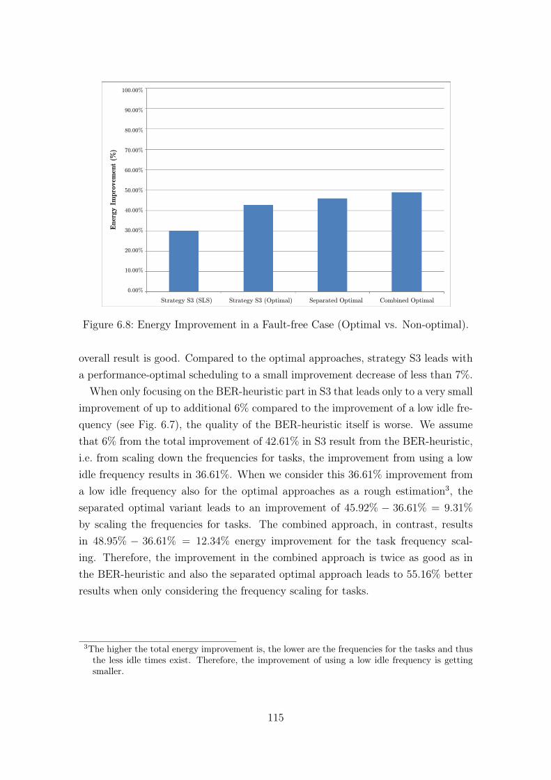
100.00%

90.00%

80.00%

70.00%

60.00%

50.00%

40.00%

30.00%

20.00%

10.00%

0.00%

Energ

y I

mpro

vem

ent

(%)

Strategy S3 (SLS) Strategy S3 (Optimal) Separated Optimal Combined Optimal

Figure 6.8: Energy Improvement in a Fault-free Case (Optimal vs. Non-optimal).

overall result is good. Compared to the optimal approaches, strategy S3 leads witha performance-optimal scheduling to a small improvement decrease of less than 7%.

When only focusing on the BER-heuristic part in S3 that leads only to a very smallimprovement of up to additional 6% compared to the improvement of a low idle fre-quency (see Fig. 6.7), the quality of the BER-heuristic itself is worse. We assumethat 6% from the total improvement of 42.61% in S3 result from the BER-heuristic,i.e. from scaling down the frequencies for tasks, the improvement from using a lowidle frequency results in 36.61%. When we consider this 36.61% improvement froma low idle frequency also for the optimal approaches as a rough estimation3, theseparated optimal variant leads to an improvement of 45.92% − 36.61% = 9.31%

by scaling the frequencies for tasks. The combined approach, in contrast, resultsin 48.95% − 36.61% = 12.34% energy improvement for the task frequency scal-ing. Therefore, the improvement in the combined approach is twice as good as inthe BER-heuristic and also the separated optimal approach leads to 55.16% betterresults when only considering the frequency scaling for tasks.

3The higher the total energy improvement is, the lower are the frequencies for the tasks and thusthe less idle times exist. Therefore, the improvement of using a low idle frequency is gettingsmaller.

115

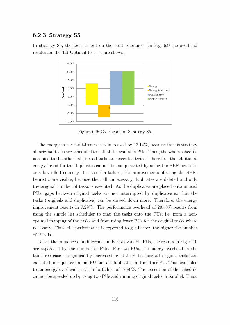
6.2.3 Strategy S5

In strategy S5, the focus is put on the fault tolerance. In Fig. 6.9 the overheadresults for the TB-Optimal test set are shown.

-10.00%

-5.00%

0.00%

5.00%

10.00%

15.00%

20.00%

25.00%

S5

Over

hea

d Energy

Energy fault case

Performance

Fault-tolerance

Figure 6.9: Overheads of Strategy S5.

The energy in the fault-free case is increased by 13.14%, because in this strategyall original tasks are scheduled to half of the available PUs. Then, the whole scheduleis copied to the other half, i.e. all tasks are executed twice. Therefore, the additionalenergy invest for the duplicates cannot be compensated by using the BER-heuristicor a low idle frequency. In case of a failure, the improvements of using the BER-heuristic are visible, because then all unnecessary duplicates are deleted and onlythe original number of tasks is executed. As the duplicates are placed onto unusedPUs, gaps between original tasks are not interrupted by duplicates so that thetasks (originals and duplicates) can be slowed down more. Therefore, the energyimprovement results in 7.29%. The performance overhead of 20.50% results fromusing the simple list scheduler to map the tasks onto the PUs, i.e. from a non-optimal mapping of the tasks and from using fewer PUs for the original tasks wherenecessary. Thus, the performance is expected to get better, the higher the numberof PUs is.

To see the influence of a different number of available PUs, the results in Fig. 6.10are separated by the number of PUs. For two PUs, the energy overhead in thefault-free case is significantly increased by 61.91% because all original tasks areexecuted in sequence on one PU and all duplicates on the other PU. This leads alsoto an energy overhead in case of a failure of 17.80%. The execution of the schedulecannot be speeded up by using two PUs and running original tasks in parallel. Thus,

116

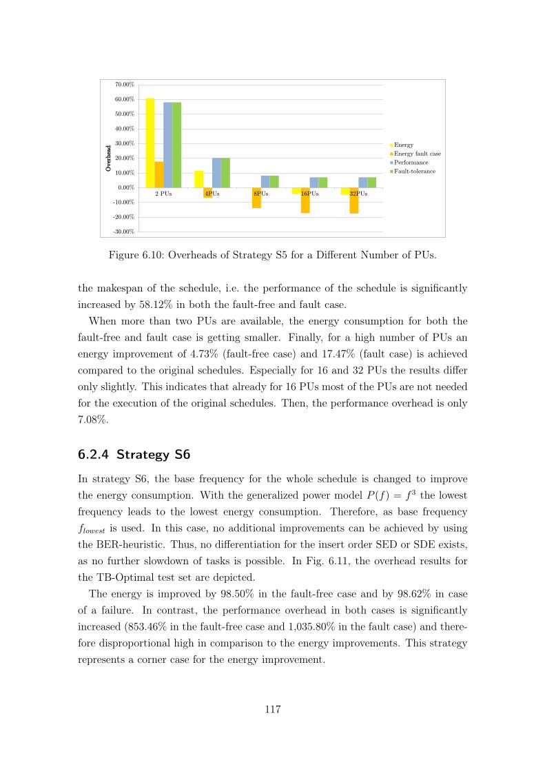
-30.00%

-20.00%

-10.00%

0.00%

10.00%

20.00%

30.00%

40.00%

50.00%

60.00%

70.00%

2 PUs 4PUs 8PUs 16PUs 32PUs

Over

hea

d Energy

Energy fault case

Performance

Fault-tolerance

Figure 6.10: Overheads of Strategy S5 for a Different Number of PUs.

the makespan of the schedule, i.e. the performance of the schedule is significantlyincreased by 58.12% in both the fault-free and fault case.

When more than two PUs are available, the energy consumption for both thefault-free and fault case is getting smaller. Finally, for a high number of PUs anenergy improvement of 4.73% (fault-free case) and 17.47% (fault case) is achievedcompared to the original schedules. Especially for 16 and 32 PUs the results differonly slightly. This indicates that already for 16 PUs most of the PUs are not neededfor the execution of the original schedules. Then, the performance overhead is only7.08%.

6.2.4 Strategy S6

In strategy S6, the base frequency for the whole schedule is changed to improvethe energy consumption. With the generalized power model P (f) = f 3 the lowestfrequency leads to the lowest energy consumption. Therefore, as base frequencyflowest is used. In this case, no additional improvements can be achieved by usingthe BER-heuristic. Thus, no differentiation for the insert order SED or SDE exists,as no further slowdown of tasks is possible. In Fig. 6.11, the overhead results forthe TB-Optimal test set are depicted.

The energy is improved by 98.50% in the fault-free case and by 98.62% in caseof a failure. In contrast, the performance overhead in both cases is significantlyincreased (853.46% in the fault-free case and 1,035.80% in the fault case) and there-fore disproportional high in comparison to the energy improvements. This strategyrepresents a corner case for the energy improvement.

117

-200.00%

0.00%

200.00%

400.00%

600.00%

800.00%

1000.00%

1200.00%

S6

Over

hea

d Energy

Energy fault case

Performance

Fault-tolerance

Figure 6.11: Overheads of Strategy S6.

6.2.5 Comparison of Strategies for the Fault-free Case

In Fig 6.12, the results for all strategies for the fault-free case (S1 to S6) are shown.

Over

hea

d

80.00%

60.00%

40.00%

20.00%

0.00%

-20.00%

-40.00%

-60.00%

Strategies

Energy

Energy fault case

Performance

Fault tolerance

1035.76% 853.46%

Impairm

ent

Impro

vem

ent

-98.50% -98.62%

S1 S2 S3 S4 S5 S6

Figure 6.12: Overheads of Different Strategies.

In all strategies, where frequency scaling is used (S3 to S6), the energy con-sumption can be improved. As expected, strategy S6 leads to the highest energyimprovements but also to the highest performance overheads in both the fault-freeand fault case. Note that the performance trends in this strategy can be totally dif-ferent for another power model as discussed in the next section with a power modelof a real system. Strategy S3 represents a good solution to improve the energy with-out decreasing the performance in a fault-free case, as the energy improvements arehigh, no performance loss in the fault-free case exists and the performance overhead

118

in case of a failure is only slightly higher compared to the other strategies S1 to S5.The best performance in case of a failure (fault-tolerance) is achieved in strategyS5 where the duplicates are executed completely in the fault-free case. In contrast,the duplicates in all other strategies are executed only partly. But in this strategy,a performance loss already exists in the fault-free case, as all tasks are scheduledwith the simple list scheduler and also only half of the PUs are used for originals.Strategy S4 can be used as an alternative for S5 as well as for S3, because the energyand performance results are between the results of S3 and S5. Thus, in strategy S4a moderate energy improvement exists but also a low performance overhead in caseof a failure.

6.2.6 Strategy S7

In strategy S7, the focus is put on the performance in the fault case. The strategy isevaluated with the test sets TB-Optimal, TB-ACO and TB-SLS. As in this strategyonly DDs are used, the performance overhead in case of a failure is compared tostrategy S3. Therefore, the focus changes form the energy in the fault-free case tothe performance in case of a failure. In Fig. 6.13 the averaged results are depicted.

0.00%

5.00%

10.00%

15.00%

20.00%

25.00%

30.00%

S3 S7

Per

form

ance

Over

hea

d in fault

case

Strategies

TB-Optimal

TB-ACO

TB-SLS

Figure 6.13: Performance Overheads in the Fault Case.

The performance overhead in case of a failure for strategy S3 is in a range of22.38% (for TB-SLS) to 28.16% (for TB-Optimal). When using the EP-heuristic inthe fault case, i.e. strategy S7, the performance overhead is decreased to 12.88% (forTB-SLS) and 16.24% (for TB-Optimal). This is an improvement of around 42%.Thus, with strategy S7 the performance is significantly increased in the fault case.

119

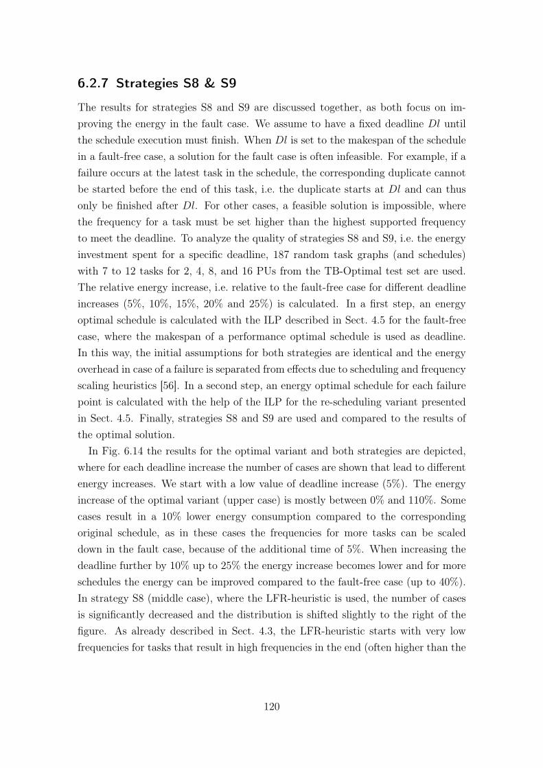
6.2.7 Strategies S8 & S9

The results for strategies S8 and S9 are discussed together, as both focus on im-proving the energy in the fault case. We assume to have a fixed deadline Dl untilthe schedule execution must finish. When Dl is set to the makespan of the schedulein a fault-free case, a solution for the fault case is often infeasible. For example, if afailure occurs at the latest task in the schedule, the corresponding duplicate cannotbe started before the end of this task, i.e. the duplicate starts at Dl and can thusonly be finished after Dl. For other cases, a feasible solution is impossible, wherethe frequency for a task must be set higher than the highest supported frequencyto meet the deadline. To analyze the quality of strategies S8 and S9, i.e. the energyinvestment spent for a specific deadline, 187 random task graphs (and schedules)with 7 to 12 tasks for 2, 4, 8, and 16 PUs from the TB-Optimal test set are used.The relative energy increase, i.e. relative to the fault-free case for different deadlineincreases (5%, 10%, 15%, 20% and 25%) is calculated. In a first step, an energyoptimal schedule is calculated with the ILP described in Sect. 4.5 for the fault-freecase, where the makespan of a performance optimal schedule is used as deadline.In this way, the initial assumptions for both strategies are identical and the energyoverhead in case of a failure is separated from effects due to scheduling and frequencyscaling heuristics [56]. In a second step, an energy optimal schedule for each failurepoint is calculated with the help of the ILP for the re-scheduling variant presentedin Sect. 4.5. Finally, strategies S8 and S9 are used and compared to the results ofthe optimal solution.

In Fig. 6.14 the results for the optimal variant and both strategies are depicted,where for each deadline increase the number of cases are shown that lead to differentenergy increases. We start with a low value of deadline increase (5%). The energyincrease of the optimal variant (upper case) is mostly between 0% and 110%. Somecases result in a 10% lower energy consumption compared to the correspondingoriginal schedule, as in these cases the frequencies for more tasks can be scaleddown in the fault case, because of the additional time of 5%. When increasing thedeadline further by 10% up to 25% the energy increase becomes lower and for moreschedules the energy can be improved compared to the fault-free case (up to 40%).In strategy S8 (middle case), where the LFR-heuristic is used, the number of casesis significantly decreased and the distribution is shifted slightly to the right of thefigure. As already described in Sect. 4.3, the LFR-heuristic starts with very lowfrequencies for tasks that result in high frequencies in the end (often higher than the

120

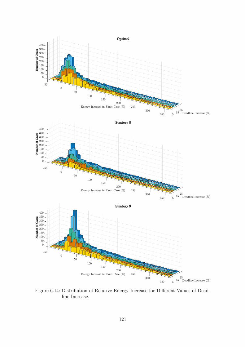
Optimal

400

350

300

250

200

150

100

50

0

Num

ber

of C

ase

s

Energy Increase in Fault Case (%)

Deadline Increase (%)

-50

0

50

100

150

200

250

300

350 5 15

25

Strategy 8

400

350

300

250

200

150

100

50

0

Num

ber

of C

ase

s

Energy Increase in Fault Case (%)

Deadline Increase (%)

-50

0

50

100

150

200

250

300

350 5 15

25

Strategy 9

400

350

300

250

200

150

100

50

0

Num

ber

of C

ase

s

Energy Increase in Fault Case (%)

Deadline Increase (%)

-50

0

50

100

150

200

250

300

350 5 15

25

Figure 6.14: Distribution of Relative Energy Increase for Different Values of Dead-line Increase.

121

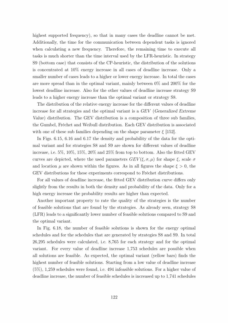
highest supported frequency), so that in many cases the deadline cannot be met.Additionally, the time for the communication between dependent tasks is ignoredwhen calculating a new frequency. Therefore, the remaining time to execute alltasks is much shorter than the time interval used by the LFR-heuristic. In strategyS9 (bottom case) that consists of the CP-heuristic, the distribution of the solutionsis concentrated at 10% energy increase in all cases of deadline increase. Only asmaller number of cases leads to a higher or lower energy increase. In total the casesare more spread than in the optimal variant, mainly between 0% and 200% for thelowest deadline increase. Also for the other values of deadline increase strategy S9leads to a higher energy increase than the optimal variant or strategy S8.

The distribution of the relative energy increase for the different values of deadlineincrease for all strategies and the optimal variant is a GEV (Generalized ExtremeValue) distribution. The GEV distribution is a composition of three sub families,the Gumbel, Fréchet and Weibull distribution. Each GEV distribution is associatedwith one of these sub families depending on the shape parameter ξ [152].In Figs. 6.15, 6.16 and 6.17 the density and probability of the data for the opti-

mal variant and for strategies S8 and S9 are shown for different values of deadlineincrease, i.e. 5%, 10%, 15%, 20% and 25% from top to bottom. Also the fitted GEVcurves are depicted, where the used parameters GEV (ξ, σ, µ) for shape ξ, scale σand location µ are shown within the figures. As in all figures the shape ξ > 0, theGEV distributions for these experiments correspond to Fréchet distributions.

For all values of deadline increase, the fitted GEV distribution curve differs onlyslightly from the results in both the density and probability of the data. Only for ahigh energy increase the probability results are higher than expected.

Another important property to rate the quality of the strategies is the numberof feasible solutions that are found by the strategies. As already seen, strategy S8(LFR) leads to a significantly lower number of feasible solutions compared to S9 andthe optimal variant.

In Fig. 6.18, the number of feasible solutions is shown for the energy optimalschedules and for the schedules that are generated by strategies S8 and S9. In total26,295 schedules were calculated, i.e. 8,765 for each strategy and for the optimalvariant. For every value of deadline increase 1,753 schedules are possible whenall solutions are feasible. As expected, the optimal variant (yellow bars) finds thehighest number of feasible solutions. Starting from a low value of deadline increase(5%), 1,259 schedules were found, i.e. 494 infeasible solutions. For a higher value ofdeadline increase, the number of feasible schedules is increased up to 1,741 schedules

122

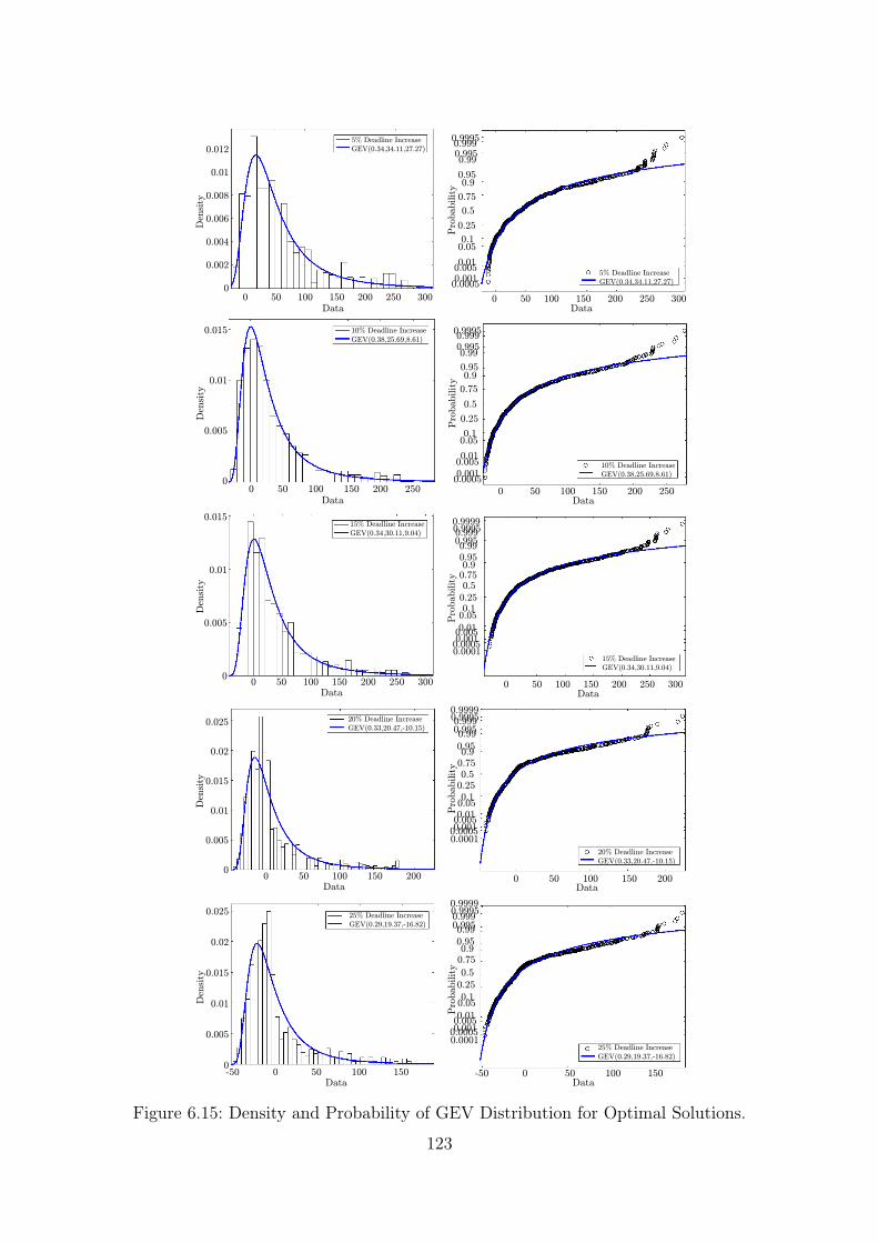
0 50 100 150 200 250 300

0.012

0.01

0.008

0.006

0.004

0.002

0

5% Deadline Increase

GEV(0.34,34.11,27.27)

Data

Den

sity

0 50 100 150 200 250 300

5% Deadline Increase

GEV(0.34,34.11,27.27)

Data

Pro

babilit

y

0.999

0.99

0.95 0.9

0.75

0.5

0.25

0.1 0.05

0.001

0.9995

0.995

0.01 0.005

0.0005

0 50 100 150 200 250

0.015

0.01

0.005

0

10% Deadline Increase

GEV(0.38,25.69,8.61)

Data

Den

sity

0 50 100 150 200 250

10% Deadline Increase

GEV(0.38,25.69,8.61)

Data

Pro

babilit

y

0.999

0.99

0.95 0.9

0.75

0.5

0.25

0.1 0.05

0.001

0.9995

0.995

0.01 0.005

0.0005

0 50 100 150 200 250 300

0.015

0.01

0.005

0

15% Deadline Increase

GEV(0.34,30.11,9.04)

Data

Den

sity

0 50 100 150 200 250 300

15% Deadline Increase

GEV(0.34,30.11,9.04)

Data

Pro

babilit

y

0.999

0.99

0.95 0.9 0.75 0.5

0.25 0.1

0.05

0.001

0.9995

0.995

0.01 0.005

0.0005

0.9999

0.0001

0 50 100 150 200

0.025

0.02

0.015

0.01

0.005

0

20% Deadline Increase

GEV(0.33,20.47,-10.15)

Data

Den

sity

0 50 100 150 200

20% Deadline Increase

GEV(0.33,20.47,-10.15)

Data

Pro

babilit

y

0.999

0.99

0.95 0.9

0.75 0.5

0.25

0.1 0.05

0.001

0.9995

0.995

0.01 0.005

0.0005

0.9999

0.0001

-50 0 50 100 150

0.025

0.02

0.015

0.01

0.005

0

25% Deadline Increase

GEV(0.29,19.37,-16.82)

Data

Den

sity

-50 0 50 100 150

25% Deadline Increase

GEV(0.29,19.37,-16.82)

Data

Pro

babilit

y

0.999

0.99

0.95 0.9

0.75

0.5

0.25

0.1 0.05

0.001

0.9995

0.995

0.01 0.005

0.0005

0.9999

0.0001

Figure 6.15: Density and Probability of GEV Distribution for Optimal Solutions.

123

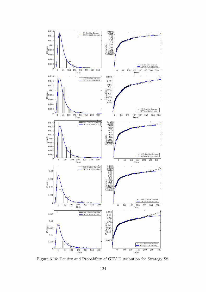
0 50 100 150 200 250 300 350

0.016

0.014

0.012

0.01

0.008

0.006

0.004

0.002

0

5% Deadline Increase

GEV(0.36,25.42,26.35)

Data

Den

sity

0 50 100 150 200 250 300 350

0.9995

5% Deadline Increase

GEV(0.36,25.42,26.35)

Data

Pro

babilit

y

0.999 0.995 0.99 0.95 0.9 0.75 0.5

0.25 0.1 0.05

0.01 0.005 0.001 0.0005 0.0001

0 50 100 150 200 250 300 350

0.016

0.014

0.012

0.01

0.008

0.006

0.004

0.002

0

10% Deadline Increase

GEV(0.28,24.54,21.52)

Data

Den

sity

0 50 100 150 200 250 300 350

10% Deadline Increase

GEV(0.28,24.54,21.52)

Data

Pro

babilit

y

0.999

0.99

0.95 0.9

0.75

0.5

0.25

0.1 0.05

0 50 100 150 200 250 300

0.018

0.016

0.014

0.012

0.01

0.008

0.006

0.004

0.002

0

15% Deadline Increase

GEV(0.34,23.85,15.43)

Data

Den

sity

0 50 100 150 200 250 300

0.9995

15% Deadline Increase

GEV(0.34,23.85,15.43)

Data

Pro

babilit

y

0.999 0.995 0.99 0.95 0.9

0.75 0.5

0.25 0.1 0.05

0.01 0.005 0.001 0.0005 0.0001

0 50 100 150 200 250 300

0.02

0.015

0.01

0.005

0

20% Deadline Increase

GEV(0.41,22.78,8.78)

Data

Den

sity

0 50 100 150 200 250 300

0.9995

20% Deadline Increase

GEV(0.41,22.78,8.78)

Data

Pro

babilit

y

0.999 0.995 0.99 0.95 0.9 0.75 0.5

0.25 0.1 0.05

0.01 0.005 0.001 0.0005 0.0001

0.9999

0 50 100 150 200 250 300

0.025

0.02

0.015

0.01

0.005

0

25% Deadline Increase

GEV(0.42,22.70,3.96)

Data

Den

sity

0 50 100 150 200 250 300

25% Deadline Increase

GEV(0.42,22.70,3.96)

Data

Pro

babilit

y

0.999

0.99

0.95 0.9 0.75

0.5

0.25 0.1

0.05

0.0001

Figure 6.16: Density and Probability of GEV Distribution for Strategy S8.

124

0 50 100 150 200 250 300 350

8

7

6

5

4

3

2

1

0

×10-3

5% Deadline Increase

GEV(0.26,49.28,47.74)

Data

Den

sity

0 50 100 150 200 250 300 350

0.9995

5% Deadline Increase

GEV(0.26,49.28,47.74)

Data

Pro

babilit

y

0.999 0.995 0.99

0.95 0.9

0.75

0.5

0.25

0.1 0.05

0.01 0.005

0.001 0.0005

0 50 100 150 200 250 300 350

0.012

0.01

0.008

0.006

0.004

0.002

0

10% Deadline Increase

GEV(0.36,36.63,28.75)

Data

Den

sity

0 50 100 150 200 250 300 350

0.9995

10% Deadline Increase

GEV(0.36,36.63,28.75)

Data

Pro

babilit

y

0.999 0.995 0.99

0.95 0.9

0.75

0.5

0.25

0.1 0.05

0.01 0.005 0.001 0.0005 0.0001

0 50 100 150 200 250 300 350 400

0.016

0.014

0.012

0.01

0.008

0.006

0.004

0.002

0

15% Deadline Increase

GEV(0.34,31.70,18.63)

Data

Den

sity

0 50 100 150 200 250 300 350 400

0.9995

15% Deadline Increase

GEV(0.34,31.70,18.63)

Data

Pro

babilit

y

0.999 0.995 0.99 0.95 0.9

0.75 0.5

0.25 0.1 0.05

0.01 0.005 0.001 0.0005 0.0001

0.9999

0 50 100 150 200 250 300 350 400

0.02

0.015

0.01

0.005

0

20% Deadline Increase

GEV(0.32,28.63,11.18)

Data

Den

sity

0 50 100 150 200 250 300 350 400

0.9995

20% Deadline Increase

GEV(0.32,28.63,11.18)

Data

Pro

babilit

y

0.999 0.995 0.99 0.95 0.9

0.75 0.5

0.25 0.1

0.05 0.01 0.005

0.001 0.0005 0.0001

0.9999

-50 0 50 100 150 200 250 300 350 400

0.025

0.02

0.015

0.01

0.005

0

25% Deadline Increase

GEV(0.28,27.20,4.89)

Data

Den

sity

-50 0 50 100 150 200 250 300 350 400

0.9995

25% Deadline Increase

GEV(0.28,28.27,4.89)

Data

Pro

babilit

y

0.999 0.995 0.99 0.95 0.9 0.75 0.5

0.25 0.1 0.05

0.01 0.005 0.001 0.0005 0.0001

0.9999

Figure 6.17: Density and Probability of GEV Distribution for Strategy S9.

125

0

200

400

600

800

1000

1200

1400

1600

1800

2000

5% DeadlineIncrease

10% DeadlineIncrease

15% DeadlineIncrease

20% DeadlineIncrease

25% DeadlineIncrease

Num

ber

of fe

asi

ble

Solu

tions

Optimal

S8 (LFR)

S9 (CP)

Figure 6.18: Number of Feasible Solutions for Different Values of Deadline Increase.

for a deadline increase of 25%, i.e. only 12 solutions were infeasible. In total 7,828out of 8,765 schedules were found. In contrast, the LFR-heuristic used in strategy S8(orange bars) leads to 2,935 out of 8,765 schedules in total. Thus, only for 33,49% ofall cases a feasible solution was found. The CP-heuristic used in strategy S9 resultsin 6,857 feasible schedules. For a low value of deadline increase (5%), 943 scheduleswere found, i.e. 316 less than in the optimal vairant. For a higher value of deadlineincrease the number of feasible solutions is increased up to 1,683 schedules at 25%deadline increase. The CP-heuristic then finds only 58 less schedules than in theoptimal variant.

In summary, the energy increase in both strategies is only moderately higher com-pared to the optimal solutions. Additionally, strategy S9 results in a high numberof feasible solutions, but strategy S8 finds no suitable solution for most of the cases.Therefore, strategy S9 is a good alternative to the optimal variant, that can befurther improved by using a more complex distribution of the power budget than asimple uniform distribution (see Sect. 4.3).

6.3 Experiments on Real World Platforms

6.3.1 Intel i7 3630qm, Intel i5 4570 and Intel i5 E1620

Model Validation To prove the accuracy of the power model explained in Sect. 5.3,three different computer systems with Intel processors are used as test platforms:

126

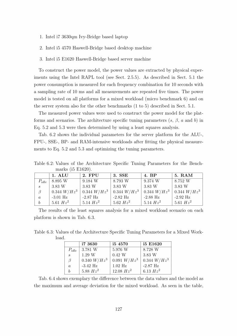
1. Intel i7 3630qm Ivy-Bridge based laptop

2. Intel i5 4570 Haswell-Bridge based desktop machine

3. Intel i5 E1620 Haswell-Bridge based server machine

To construct the power model, the power values are extracted by physical exper-iments using the Intel RAPL tool (see Sect. 2.5.5). As described in Sect. 5.1 thepower consumption is measured for each frequency combination for 10 seconds witha sampling rate of 10 ms and all measurements are repeated five times. The powermodel is tested on all platforms for a mixed workload (micro benchmark 6) and onthe server system also for the other benchmarks (1 to 5) described in Sect. 5.1.

The measured power values were used to construct the power model for the plat-forms and scenarios. The architecture specific tuning parameters (s, β, a and b) inEq. 5.2 and 5.3 were then determined by using a least squares analysis.

Tab. 6.2 shows the individual parameters for the server platform for the ALU-,FPU-, SSE-, BP- and RAM-intensive workloads after fitting the physical measure-ments to Eq. 5.2 and 5.3 and optimizing the tuning parameters.

Table 6.2: Values of the Architecture Specific Tuning Parameters for the Bench-marks (i5 E1620).

1. ALU 2. FPU 3. SSE 4. BP 5. RAMPidle 8.895 W 9.184 W 8.793 W 9.374 W 8.752 Ws 3.83 W 3.83 W 3.83 W 3.83 W 3.83 Wβ 0.344 W/Hz3 0.344 W/Hz3 0.344 W/Hz3 0.344 W/Hz3 0.344 W/Hz3

a -3.01 Hz -2.87 Hz -2.82 Hz -2.88 Hz -2.92 Hzb 5.61 Hz2 5.14 Hz2 5.62 Hz2 5.14 Hz2 5.61 Hz2

The results of the least squares analysis for a mixed workload scenario on eachplatform is shown in Tab. 6.3.

Table 6.3: Values of the Architecture Specific Tuning Parameters for a Mixed Work-load.

i7 3630 i5 4570 i5 E1620Pidle 3.781 W 5.976 W 8.728 Ws 1.29 W 0.42 W 3.83 Wβ 0.340 W/Hz3 0.091 W/Hz3 0.344 W/Hz3

a -3.42 Hz 1.02 Hz -2.87 Hzb 5.88 Hz2 12.08 Hz2 6.13 Hz2

Tab. 6.4 shows exemplary the difference between the data values and the model asthe maximum and average deviation for the mixed workload. As seen in the table,

127

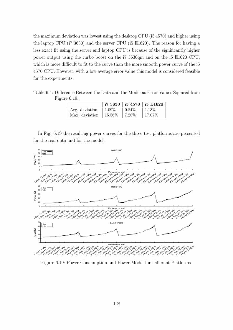
the maximum deviation was lowest using the desktop CPU (i5 4570) and higher usingthe laptop CPU (i7 3630) and the server CPU (i5 E1620). The reason for having aless exact fit using the server and laptop CPU is because of the significantly higherpower output using the turbo boost on the i7 3630qm and on the i5 E1620 CPU,which is more difficult to fit to the curve than the more smooth power curve of the i54570 CPU. However, with a low average error value this model is considered feasiblefor the experiments.

Table 6.4: Difference Between the Data and the Model as Error Values Squared fromFigure 6.19.

i7 3630 i5 4570 i5 E1620Avg. deviation 1.09% 0.84% 1.13%Max. deviation 15.56% 7.28% 17.07%

In Fig. 6.19 the resulting power curves for the three test platforms are presentedfor the real data and for the model.

0

5

10

15

20

25

30

1 Core 1.3 G

Hz

1 Core 1.5 G

Hz

1 Core 1.7 G

Hz

1 Core 1.9 G

Hz

1 Core 2.1 G

Hz

1 Core 2.3 G

Hz

1 Core 3.4 G

Hz

2 Cores 1

.3 GHz

2 Cores 1

.5 GHz

2 Cores 1

.7 GHz

2 Cores 1

.9 GHz

2 Cores 2

.1 Ghz

2 Cores 2

.3 GHz

2 Cores 3

.3 GHz

3 Cores 1

.3 GHz

3 Cores 1

.5 GHz

3 Cores 1

.7 GHz

3 Cores 1

.9 GHz

3 Cores 2

.1 GHz

3 Cores 2

.3 GHz

3 Cores 3

.2 GHz

4 Cores 1

.3 GHz

4 Cores 1

.5 GHz

4 Cores 1

.7 GHz

4 Cores 1

.9 GHz

4 Cores 2

.1 GHz

4 Cores 2

.3 GHz

4 Cores 3

.2 GHz

Po

we

r [W

]

Performance level

Intel i7 3630DataModel

0

10

20

30

40

50

1 Core 1.0 G

Hz

1 Core 1.3 G

Hz

1 Core 1.7 G

Hz

1 Core 2.0 G

Hz

1 Core 2.3 G

Hz

1 Core 2.7 G

Hz

1 Core 3.0 G

Hz

1 Core 3.6 G

Hz

2 Cores 1

.0 GHz

2 Cores 1

.3 GHz

2 Cores 1

.7 GHz

2 Cores 2

.0 GHz

2 Cores 2

.3 GHz

2 Cores 2

.7 GHz

2 Cores 3

.0 GHz

2 Cores 3

.6 GHz

3 Cores 1

.0 GHz

3 Cores 1

.3 GHz

3 Cores 1

.7 GHz

3 Cores 2

.0 GHz

3 Cores 2

.3 GHz

3 Cores 2

.7 GHz

3 Cores 3

.0 GHz

3 Cores 3

.6 GHz

4 Cores 1

.0 GHz

4 Cores 1

.3 GHz

4 Cores 1

.7 GHz

4 Cores 2

.0 GHz

4 Cores 2

.3 GHz

4 Cores 2

.7 GHz

4 Cores 3

.0 GHz

4 Cores 3

.6 GHz

Po

we

r [W

]

Performance level

Intel i5 4570DataModel

0

10

20

30

40

50

1 Core 1.4 G

Hz

1 Core 1.7 G

Hz

1 Core 2.0 G

Hz

1 Core 2.3 G

Hz

1 Core 2.7 G

Hz

1 Core 3.0 G

Hz

1 Core 3.3 G

Hz

1 Core 3.6 G

Hz

2 Cores 1

.4 GHz

2 Cores 1

.7 GHz

2 Cores 2

.0 GHz

2 Cores 2

.3 GHz

2 Cores 2

.7 GHz

2 Cores 3

.0 GHz

2 Cores 3

.3 GHz

2 Cores 3

.6 GHz

3 Cores 1

.4 GHz

3 Cores 1

.7 GHz

3 Cores 2

.0 GHz

3 Cores 2

.3 GHz

3 Cores 2

.7 GHz

3 Cores 3

.0 GHz

3 Cores 3

.3 GHz

3 Cores 3

.6 GHz

4 Cores 1

.4 GHz

4 Cores 1

.7 GHz

4 Cores 2

.0 GHz

4 Cores 2

.3 GHz

4 Cores 2

.7 GHz

4 Cores 3

.0 GHz

4 Cores 3

.3 GHz

4 Cores 3

.6 GHz

Po

we

r [W

]

Performance level

Intel i5 E1620DataModel

Figure 6.19: Power Consumption and Power Model for Different Platforms.

128

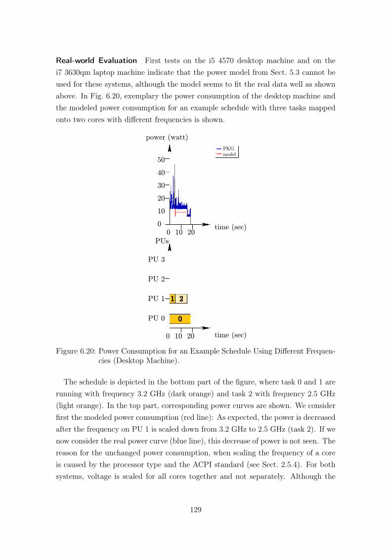
Real-world Evaluation First tests on the i5 4570 desktop machine and on thei7 3630qm laptop machine indicate that the power model from Sect. 5.3 cannot beused for these systems, although the model seems to fit the real data well as shownabove. In Fig. 6.20, exemplary the power consumption of the desktop machine andthe modeled power consumption for an example schedule with three tasks mappedonto two cores with different frequencies is shown.

50

40

30

20

10

0

PU 3

PU 2

PU 1

PU 0

0 10 20

0 10 20 time (sec)

time (sec)

PUs

power (watt)

PKG

model

0

1 2

Figure 6.20: Power Consumption for an Example Schedule Using Different Frequen-cies (Desktop Machine).

The schedule is depicted in the bottom part of the figure, where task 0 and 1 arerunning with frequency 3.2 GHz (dark orange) and task 2 with frequency 2.5 GHz(light orange). In the top part, corresponding power curves are shown. We considerfirst the modeled power consumption (red line): As expected, the power is decreasedafter the frequency on PU 1 is scaled down from 3.2 GHz to 2.5 GHz (task 2). If wenow consider the real power curve (blue line), this decrease of power is not seen. Thereason for the unchanged power consumption, when scaling the frequency of a coreis caused by the processor type and the ACPI standard (see Sect. 2.5.4). For bothsystems, voltage is scaled for all cores together and not separately. Although the

129

total voltage might be decreased depending on the frequencies, the ACPI standardforces the system to use a voltage level high enough to let all active cores runningon the highest frequency in use. Hence, as long as not all cores are scaled down,the voltage level is kept high. After task 0 and task 2 have finished, the powerconsumption is, as expected, decreased to the idle power of around 6 W. As thesystem check tool (see Sect. 5.1) does not measure power consumption for differentfrequencies at the same time, i.e. only one frequency for a different number of activecores, the above explained behavior was not identified by this tool.

The behavior of the power consumption on the server system differs from the othersystems, as now for each core a separate voltage regulator is used independently.Fig. 6.21 shows an example test case, where the expected behavior, i.e. the modeledpower consumption fits the real power consumption well4.

40

30

20

10

0

PU 3

PU 2

PU 1

PU 0

0 10 20 30 40 50 60 70 80 90 100 110 120 130 140 150 160

time (sec)

time (sec)

PUs

power (watt)

PKG

model

0 7 8 10 11 12 17 18

0 10 20 30 40 50 60 70 80 90 100 110 120 130 140 150 160

2 14 15 19 16 20

1 4 5 3 9 13 15 19 20

2 8 11 12

6 14 16

1 04 10 9 13

7 5 6 3 17 18

original task

(dummy) duplicate

Figure 6.21: Power Consumption for an Example Schedule Using Different Frequen-cies (Server Machine).

4This figure was generated automatically by a developed figure generator that is included intothe runtime system RUPS, to check (in an easy way) the correct behavior of the real system inuse.

130

In this example, a fault-tolerant schedule is depicted that was executed in a fault-free case. The red tasks represent the duplicates (in this case only DDs are used) anddifferent frequencies are indicated by different shades of orange. A darker orangerepresents a higher frequency, a lighter orange a lower frequency.

The server system as a common platform for clusters and grids is therefore used forthe real-world evaluation. For each workload scenario, 922 schedules were tested thatare related to 40 task graphs from the TB-Optimal test set with random propertiesand between 19 and 24 tasks. For each task graph the already existing schedule runsfirstly without any changes and thus without any failures. Then, the fault-tolerantschedules that result from strategy S3, where only DDs and the BER-heuristic areused (see Sect. 4.4.2) were calculated and executed by the runtime system. Then,all fault-tolerant schedules run with a simulated failure at each task by exiting thecorresponding MPI-Process directly before the task execution started.

The accuracy of the prediction is validated by comparing the predicted energyvalues that result from the scheduler with the real measurements of the runtimesystem.

In Fig. 6.22, exemplary the predicted and real energy consumption for a mixedworkload for all schedules is presented.

6500

6000

5500

5000

4500

4000

3500

3000

2500

Ener

gy (

J)

0 100 200 300 400 500 600 700 800 900 1000

Schedule Nr.

Predicted Energy

Measured Energy

Figure 6.22: Comparison Between Predicted and Measured Energy Consumption(for Mixed Workloads).

131

Tab. 6.5 presents the averaged and maximum deviation for the prediction for allbenchmarks. With a maximum deviation of around 7.73% and nearly 2.24% onaverage, the prediction fits the reality quite well.

Table 6.5: Differences Between Measured Data and Predictions for all Schedules.Deviation Prediction

Average Maximum1. ALU 2.42% 7.63%2. FPU 2.00% 7.33%3. SSE 1.81% 7.75%4. BP 3.45 8.61%5. RAM 2.09% 7.90%6. Mixed (all tests) 1.64% 7.14%In total (averaged) 2.24% 7.73%

Upper/Lower Bounds for the Energy Consumption The estimation of upperand lower bounds for PE and FT in Sect. 3.4 are independent of a certain system.They are correct in general for every system. But the estimation of the upper andlower bounds for E depends highly on the system in use. In Sect. 3.4, these boundsare estimated for a generalized power model. Therefore, the bounds have to beadapted to the server system by considering the measured values resulting from thesystem check tool for the estimation. Based on these values, the energy consumptionof the i5 E1620 processor is calculated for a workload at different frequencies andnumber of cores. We assume a perfectly divisible workload can be executed in onesecond when using 4 cores and the highest supported frequency (3.6 GHz). Basedon this assumption, the runtime of the workload for all other frequency/core com-binations can be calculated. Then, the energy consumption for the workload can beachieved by multiplying the calculated runtime with the measured power consump-tion for the corresponding frequency and number of active cores. In Fig. 6.23, theenergy behavior for the server system is presented.

The lowest energy consumption is at 2.3 GHz using four cores, the highest energyconsumption is at the lowest frequency (1.2 GHz) using one core. Thus, a lowerbound for E can be given by:

Ebest =mseq

pmax · 2.3 GHz. (6.1)

132

Intel i5 E 1620 1 Core

2 Cores

3 Cores

4 Cores

180

160

140

120

100

80

60

40

20

0

Ener

gy (

J)

1.2 1.4 1.5 1.7 1.9 2 2.2 2.3 2.5 2.7 2.8 3 3.2 3.3 3.5 3.6

Frequency (GHz)

Figure 6.23: Energy Behavior for a Workload at Different Frequencies and Numberof Cores.

An upper bound for E can be achieved by running all tasks in sequence on onePU with the lowest possible frequency flowest:

Eworst =mseq

1 · flowest. (6.2)

Results The experiments are done with the TB-Optimal test set. As seen above,the system model closely reflects the real system in terms of energy consumption.This fact is used to simulate nearly 34,500 of the given schedules using the RUPSsystem. The trade-off between PE, FT , and E is evaluated with the four strategiesS3 to S6 from Sect. 4.4.2. These strategies reflect system setups with one of thethree parameters as inherently dominating. This choice will give a wide range of ex-periments with the extreme corner cases covered and everything between the cornercases. In all strategies, the BER-heuristic is used to reduce the energy consumption.The following strategies were used for the simulation, where the turbo frequency isnot considered to avoid throttling effects:

S3: Use only DDs and start with the second highest supported frequency (3.5GHz). In this scenario, the focus is firstly put on PE and secondly on E.

S4: Use Ds and DDs and start with the second highest supported frequency (3.5GHz). This scenario mainly targets on PE, but also on FT .

133

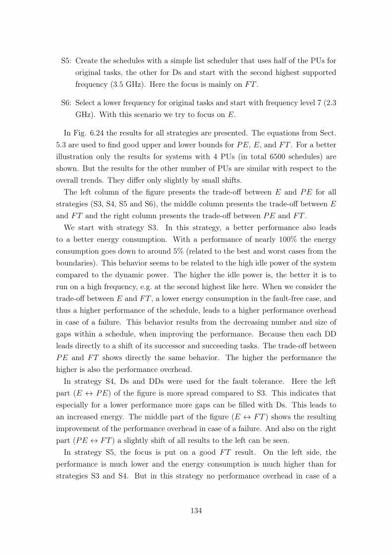
S5: Create the schedules with a simple list scheduler that uses half of the PUs fororiginal tasks, the other for Ds and start with the second highest supportedfrequency (3.5 GHz). Here the focus is mainly on FT .

S6: Select a lower frequency for original tasks and start with frequency level 7 (2.3GHz). With this scenario we try to focus on E.

In Fig. 6.24 the results for all strategies are presented. The equations from Sect.5.3 are used to find good upper and lower bounds for PE, E, and FT . For a betterillustration only the results for systems with 4 PUs (in total 6500 schedules) areshown. But the results for the other number of PUs are similar with respect to theoverall trends. They differ only slightly by small shifts.

The left column of the figure presents the trade-off between E and PE for allstrategies (S3, S4, S5 and S6), the middle column presents the trade-off between Eand FT and the right column presents the trade-off between PE and FT .We start with strategy S3. In this strategy, a better performance also leads

to a better energy consumption. With a performance of nearly 100% the energyconsumption goes down to around 5% (related to the best and worst cases from theboundaries). This behavior seems to be related to the high idle power of the systemcompared to the dynamic power. The higher the idle power is, the better it is torun on a high frequency, e.g. at the second highest like here. When we consider thetrade-off between E and FT , a lower energy consumption in the fault-free case, andthus a higher performance of the schedule, leads to a higher performance overheadin case of a failure. This behavior results from the decreasing number and size ofgaps within a schedule, when improving the performance. Because then each DDleads directly to a shift of its successor and succeeding tasks. The trade-off betweenPE and FT shows directly the same behavior. The higher the performance thehigher is also the performance overhead.

In strategy S4, Ds and DDs were used for the fault tolerance. Here the leftpart (E ↔ PE) of the figure is more spread compared to S3. This indicates thatespecially for a lower performance more gaps can be filled with Ds. This leads toan increased energy. The middle part of the figure (E ↔ FT ) shows the resultingimprovement of the performance overhead in case of a failure. And also on the rightpart (PE ↔ FT ) a slightly shift of all results to the left can be seen.

In strategy S5, the focus is put on a good FT result. On the left side, theperformance is much lower and the energy consumption is much higher than forstrategies S3 and S4. But in this strategy no performance overhead in case of a

134

failure exists. Therefore, the middle and right boxes of the figure are empty and theperformance in the fault case is equal to the performance in the fault-free case.

Strategy S6 is used to generate schedules that run with a lower frequency (fre-quency level 7, 2.3 GHz). The energy consumption can be improved by running ona lower frequency, bot only if the performance is increased. Then, nearly the bestenergy consumption of 0%, i.e. the lower bound of E can be reached. The otherboth trade-offs are the same like for strategy S3. They are just a little bit stretched.

50 60 70 80 90 100

50 60 70 80 90 100

50 60 70 80 90 100

50 60 70 80 90 100 0 20 40 60 80 100

0 20 40 60 80 100

0 20 40 60 80 100

0 20 40 60 80 100

0 20 40 60 80 100

0 20 40 60 80 100

0 20 40 60 80 100

0 20 40 60 80 100 Performance (%)

Performance (%)

Performance (%)

Performance (%)

Performance Overhead

when Fault (%)

Performance Overhead

when Fault (%)

Performance Overhead

when Fault (%)

Performance Overhead

when Fault (%)

Performance Overhead

when Fault (%)

Performance Overhead

when Fault (%)

Performance Overhead

when Fault (%)

Performance Overhead

when Fault (%)

Rel

ative

Ener

gy

Consu

mption

Per

form

ance

(%

) P

erfo

rmance

(%

) P

erfo

rmance

(%

) P

erfo

rmance

(%

)

Rel

ative

Ener

gy

Consu

mption

Rel

ative

Ener

gy

Consu

mption

Rel

ative

Ener

gy

Consu

mption

Rel

ative

Ener

gy

Consu

mption

Rel

ative

Ener

gy

Consu

mption

Rel

ative

Ener

gy

Consu

mption

Rel

ative

Ener

gy

Consu

mption

60

50

40

30

20

10

0

60

50

40

30

20

10

0

60

50

40

30

20

10

0

60

50

40

30

20

10

0

60

50

40

30

20

10

0

60

50

40

30

20

10

0

60

50

40

30

20

10

0

60

50

40

30

20

10

0

100

90

80

70

60

50

100

90

80

70

60

50

100

90

80

70

60

50

100

90

80

70

60

50

S3

S4

S5

S6

Figure 6.24: Results when Scheduling According to Scenarios A,B,C,D Showing:Relative Energy Consumption (Lower is Better), Performance (Higheris Better), Performance Overhead when Fault (Lower is Better).

135

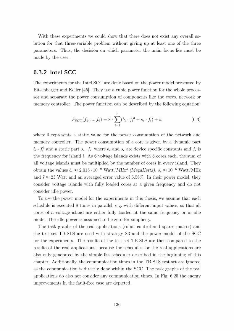
With these experiments we could show that there does not exist any overall so-lution for that three-variable problem without giving up at least one of the threeparameters. Thus, the decision on which parameter the main focus lies must bemade by the user.

6.3.2 Intel SCC

The experiments for the Intel SCC are done based on the power model presented byEitschberger and Keller [45]. They use a cubic power function for the whole proces-sor and separate the power consumption of components like the cores, network ormemory controller. The power function can be described by the following equation:

PSCC(f1, ..., f6) = 8 ·6∑i=1

(bc · fi3 + sc · fi) + s̃, (6.3)

where s̃ represents a static value for the power consumption of the network andmemory controller. The power consumption of a core is given by a dynamic partbc · f 3

i and a static part sc · fi, where bc and sc are device specific constants and fi isthe frequency for island i. As 6 voltage islands exists with 8 cores each, the sum ofall voltage islands must be multiplied by the number of cores in every island. Theyobtain the values bc ≈ 2.015 · 10−9 Watt/MHz3 (MegaHertz), sc ≈ 10−6 Watt/MHzand s̃ ≈ 23 Watt and an averaged error value of 5.58%. In their power model, theyconsider voltage islands with fully loaded cores at a given frequency and do notconsider idle power.

To use the power model for the experiments in this thesis, we assume that eachschedule is executed 8 times in parallel, e.g. with different input values, so that allcores of a voltage island are either fully loaded at the same frequency or in idlemode. The idle power is assumed to be zero for simplicity.

The task graphs of the real applications (robot control and sparse matrix) andthe test set TB-SLS are used with strategy S3 and the power model of the SCCfor the experiments. The results of the test set TB-SLS are then compared to theresults of the real applications, because the schedules for the real applications arealso only generated by the simple list scheduler described in the beginning of thischapter. Additionally, the communication times in the TB-SLS test set are ignoredas the communication is directly done within the SCC. The task graphs of the realapplications do also not consider any communication times. In Fig. 6.25 the energyimprovements in the fault-free case are depicted.

136

0.00%

1.00%

2.00%

3.00%

4.00%

5.00%

6.00%

7.00%

8.00%

9.00%

10.00%

Robot Sparse Matrix TB-SLS(no communication time)

Ener

gy I

mpro

vem

ent

(%)

Figure 6.25: Energy Improvement in a Fault-free Case (Strategy S3).

For the SCC as an example of a manycore system and task graphs without com-munication costs, the energy can be improved by around 2% for the real applicationsand by 3.93% for the TB-SLS test set without communication costs.

6.4 Analysis of the Scheduling Time

The averaged and maximum scheduling time to generate a schedule is shown inTab. 6.6.

Table 6.6: Scheduling Time.Schedules with Schedules with Schedules with7-24 Tasks 25 - 250 Tasks 7 - 12 Tasks(heuristics) (heuristics) (optimal)

Average 0.038 s 11.27 s 21.63 sMaximum 8.78 s 194.31 s 1,723.14 s

For the test sets TB-Optimal, TB-ACO and TB-SLS with a small number oftasks (7 - 24 tasks), the averaged scheduling time is very low (0.038 s). Even themaximum scheduling time of 8.78 seconds is moderate compared to the runtime ofa schedule (of around 120 s on average). For all strategies the scheduling time forthe small cases varies in a small range of 0.029 s and 0.053 s, where the lower valueswere achieved in strategies S1 to S4.

137

The scheduling time for the large cases with up to 250 tasks is on average at 11.27s. The maximum is at 194.31 s. Also here the scheduling time is small compared tothe runtime of a schedule (of around 1000 s on average).

In contrast, the scheduling time for the optimal solutions for 7 - 12 tasks is veryhigh with 21.63 s on average and with a maximum of 1,723.14 s. Especially forschedules with a high number of PUs the solution space is significantly increased.The time for the generation of optimal solutions is therefore disproportional highcompared to the improvements resulting from the optimization.

6.5 Summary & Discussion

In this chapter, the proposed strategies from Sect. 4.4 were evaluated and analyzedfor various power models and platforms. As a result, the accuracy of the powermodel for parallel platforms, presented in Sect. 5.3, is on average quite well witha standard deviation of around 1% (see Sect. 6.3.1). For processors with separatevoltage regulators for each core like the Intel i5 E1620, the prediction of the scheduler(and simulator) is close to the real behavior. Only small standard deviations of2.24% (on average) and 7.73% (on maximum) exist. Different types of workloadscan be considered by using various workload classes, as proposed in Sect. 5.1, andcorresponding parameters for the power model, as presented in Sect. 6.3.1.

If the frequency of PUs is constant over the whole schedule execution, the use ofavailable and free PUs for the placement of duplicates leads to a better performancebut to a significant higher energy consumption. However, if frequency scaling issupported by the parallel system, most of the energy improvements result from idletimes where the frequency is scaled down to the lowest possible. In addition, upto 6% can be saved, when the frequency for tasks is scaled, too (see Sect. 6.2.2).A combined optimization of performance and energy consumption is slightly betterthan a separated optimization. Compared to solutions with an optimal classicalscheduling and strategy S3 for reducing the energy consumption, the difference issmall. Hence, using S3 is a good alternative to the optimal solutions.

If the focus of a user is put on the fault tolerance, strategy S5 is advantageous forhigh numbers of PUs. For small numbers of PUs, strategy S4 leads to better results.

Strategy S6 with the highest energy savings is worthwhile for parallel platforms,where the most energy efficient frequency is in the upper range of the supportedfrequencies. Otherwise, the performance decrease is disproportional high so thatthen strategy S3 is the better choice.

138

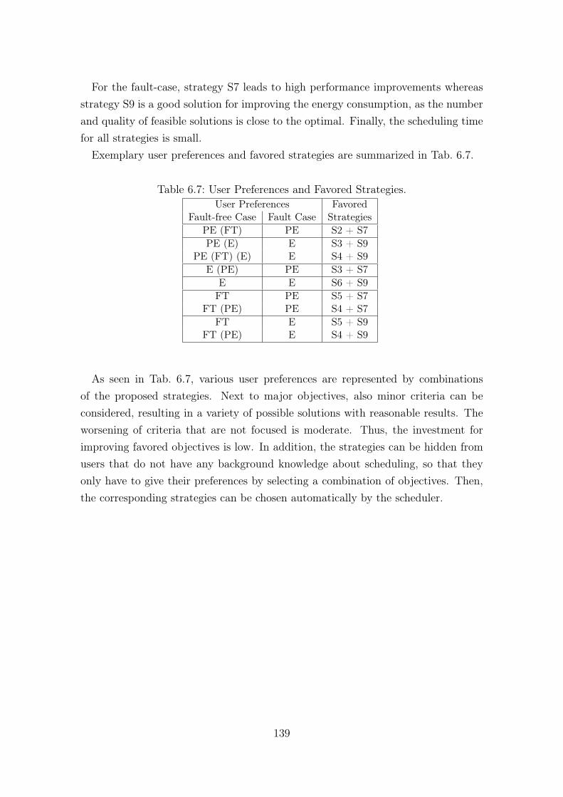
For the fault-case, strategy S7 leads to high performance improvements whereasstrategy S9 is a good solution for improving the energy consumption, as the numberand quality of feasible solutions is close to the optimal. Finally, the scheduling timefor all strategies is small.

Exemplary user preferences and favored strategies are summarized in Tab. 6.7.

Table 6.7: User Preferences and Favored Strategies.User Preferences Favored

Fault-free Case Fault Case StrategiesPE (FT) PE S2 + S7PE (E) E S3 + S9

PE (FT) (E) E S4 + S9E (PE) PE S3 + S7

E E S6 + S9FT PE S5 + S7

FT (PE) PE S4 + S7FT E S5 + S9

FT (PE) E S4 + S9

As seen in Tab. 6.7, various user preferences are represented by combinationsof the proposed strategies. Next to major objectives, also minor criteria can beconsidered, resulting in a variety of possible solutions with reasonable results. Theworsening of criteria that are not focused is moderate. Thus, the investment forimproving favored objectives is low. In addition, the strategies can be hidden fromusers that do not have any background knowledge about scheduling, so that theyonly have to give their preferences by selecting a combination of objectives. Then,the corresponding strategies can be chosen automatically by the scheduler.

139

140

7 Conclusions

In this thesis, the interplay between performance, fault tolerance and energy con-sumption was explored. In general, an overall optimal solution for this three-dimensional optimization problem does not exist. All two-dimensional combinationsof the above mentioned objectives already result in a trade-off, where the improve-ment of one criterion leads to a worsening of the other one. In the literature, thefocus is therefore often put on one criterion that is improved, while the other oneis fixed. For example, the energy consumption for a schedule is optimized withoutchanging the performance. A combination of all three above mentioned objectivesis even more complex, since a change of an objective no longer affects only anotherbut also can affect both other objectives. In the literature, the three-dimensionaloptimization is rarely considered. Often, the focus on the primary and secondarycriterion is already fixed in advance. However, as a result, only a very small partof the total view of the trade-off is addressed on the one hand, and also no otherorientations are considered on the other hand.

To discuss the trade-off between the three objectives in detail, in this thesis severalfault-tolerant and energy-efficient strategies were presented that focus on differentcriteria in the fault-free case and ultimately represent several preferences of a user.Therefore, the fault-tolerant task duplication-based scheduling approach of Fechneret al. [59] is used, extended and combined with energy-efficient options and heuris-tics. Additionally, another trade-off between the fault-free and fault case is notaddressed in previous work. But the preferences of a user can change between bothcases. For example in a fault-free case, the energy consumption is the most impor-tant criterion, while in the fault case the performance is dominating. Therefore, inthis work also strategies for the fault case were presented that either focus on theperformance or on the energy consumption. In addition, energy-optimal solutionswere presented and used for comparison.

The strategies were evaluated with various test sets from the benchmark suite ofHönig [84]. In a first step, the energy consumption for the resulting schedules waspredicted based on a generalized power model, independently of a certain platform.

141

In a second step, power models for real parallel platforms with an acceptable accu-racy were constructed, tested and used in the evaluation. Therefore, in this worka fault-tolerant and energy-efficient prototype runtime system called RUPS (Run-time system for User Preferences-defined Schedules) was presented, that is realizedwith an extended fault-tolerant version of MPI and supports frequency scaling byintegrating DVFS.

To analyze and visualize the trade-off between all objectives, the performanceand energy consumption for all strategies were given for both the fault-free andfault case. The results show, that various factors have a significant influence on thetrade-off like different energy curves of processors, the number of used PUs for theplacement of duplicates or a tolerable increase of the makespan in case of a failure.In terms of energy, the most improvements result from idle times, where a lowestsupported frequency can be used and only a smaller part can be achieved by alsoscaling frequencies for tasks.

142

8 Outlook

As in this thesis several subjects like performance, fault tolerance, energy efficiency,heuristics, optimization, power modeling, or runtime system are combined under abroader topic, a wide spectrum of future research can be done. Therefore, only somepossible directions are described in the following:

Performance In this thesis only homogeneous systems are considered. An exten-sion to heterogeneous systems can be included to get more possibilities to improvethe performance of a schedule. Until now, the CBF-heuristic is only implementedfor the fault-free case. Therefore, the implementation for the fault case can be doneto also speedup the whole schedule, i.e. the performance of the schedule in case ofa failure. The EP-heuristic can be improved by also allowing tasks to start earlierthan the time given in the static schedule.

Fault tolerance The probability of a fault or failure depending on the runtimeof a task, schedule, or PU is not considered. Tasks for example can be weightedaccording to their runtime, so that longer running tasks get a higher probabilityto fail. Another aspect focuses on the number of failures, that can be toleratedby the runtime system. Mainly two possibilities exist: Including more copies ofeach original task, i.e. duplicates directly in the fault-free case into the schedule ordelete all unnecessary duplicates in case of a failure and include a new duplicate foreach task. The first approach might lead to a lower performance in case of morethan one failure because of an inefficient placement of the duplicates, the secondapproach in contrast is a hybrid approach where the duplicates after a failure areincluded dynamically during the runtime of a schedule and therefore lead to a lowerperformance, but also to a better placement of duplicates. Additionally, the secondapproach is in contrast to the first approach restricted to only one failure at a time.In this work only permanent faults (failures) are considered. Another extensioncould be to include also the toleration of temporary faults, where a PU is availableagain after some time.

143

Energy Efficiency The energy consumption in case of a failure can be improvedfor strategy S9 by using a more complex distribution for the power budget. Thenumber of feasible solutions for strategy S8 and also the energy consumption incase of a failure can be improved by considering a certain percentage value for thecommunication time when calculating a new frequency. As the scheduling time ofstrategies S7 - S9 is small compared to the schedule runtime, another approach isto calculate the energy and makespan for all strategies in the fault case and choosethe best one according to the users’ preferences. Another approach to save energycan be done by considering also the frequency scaling for the network in use. Forexample, the Intel SCC offers 2 frequency levels for the network: 800 MHz and 1600MHz.

Optimization One question that arose during the creation of the ILPs in thiswork, but that is not considered in this thesis is, if it is possible to find the max-imum number of PUs necessary for an energy optimal solution with the help ofthe information from a performance optimal solution and the task graph when thedeadline is set to the makespan of the performance optimal schedule. For example,the number of PUs for an energy optimal solution must be at least as high as thenumber of the performance optimal solution, because otherwise the schedule wouldbe prolonged and thus the deadline cannot be met. On the other side, an energyoptimal solution might need more PUs than the performance optimal solution toget more possibilities to scale down tasks.

Power Modeling In this thesis a very simple power model is used for the intelprocessors. This model might be improved by including more details into this model.Also other components of a computer system might be included into the overallenergy rating, like the energy consumption for the memory controller or for thehard disks. Another possibility is to find a power model for processors, that have noseparate voltage regulators like the discussed i5 desktop processor or the i7 laptopprocessor. Then, new strategies and heuristics can be implemented, that considerfrequency scaling only for all cores together and not independently.

Runtime System The prototype runtime system can be extended by includingcomplete messages for the communication and not only the message header. Addi-tionally, the runtime system can be adapted to support real applications based ona task graph instead of simulated workloads.

144

Bibliography

[1] J. H. Abawajy, “Fault-tolerant Scheduling Policy for Grid Computing Sys-tems,” in Proceedings of the 18th International Parallel and Distributed Pro-cessing Symposium (IPDPS ’04). IEEE, 2004, pp. 238–245.

[2] T. L. Adam, K. M. Chandy, and J. Dickson, “A Comparison of List Schedulesfor Parallel Processing Systems,” Communications of the ACM, vol. 17, no. 12,pp. 685–690, 1974.

[3] N. Agarwal, P. Chauhan, and D. Nitin, “Fault-tolerant Heterogeneous Lim-ited Duplication Scheduling Algorithm for Decentralized Grid,” InternationalJournal of Computers & Technology (IJCT), vol. 4, no. 3, pp. 765–775, 2013.

[4] I. Ahmad, Y.-K. Kwok, and M.-Y. Wu, “Analysis, Evaluation, and Com-parison of Algorithms for Scheduling Task Graphs on Parallel Processors,”in Proceedings of the 2nd International Symposium on Parallel Architectures,Algorithms, and Networks (I-SPAN ’96), Jun 1996, pp. 207–213.

[5] K. Ahn, J. Kim, and S. Hong, “Fault-tolerant Real-time Scheduling UsingPassive Replicas,” in Proceedings of the Pacific Rim International Symposiumon Fault-Tolerant Systems (PRFTS ’97). IEEE, 1997, pp. 98–103.

[6] B. Alam and A. Kumar, “Fault Tolerance Issues in Real Time Systems withEnergy Minimization,” International Journal of Information and ComputationTechnology (IJICT), vol. 3, no. 10, pp. 1001–1008, 2013.

[7] S. Albers, “Energy-efficient Algorithms,” Communications of the ACM,vol. 53, no. 5, pp. 86–96, May 2010. [Online]. Available: http://doi.acm.org/10.1145/1735223.1735245

[8] D. G. Amalarethinam and G. J. Mary, “A New DAG-based Dynamic TaskScheduling Algorithm (DYTAS) for Multiprocessor Systems,” InternationalJournal of Computer Applications, vol. 19, no. 8, pp. 24–28, April 2011.

i

[9] P. R. Amestoy, A. Guermouche, J.-Y. L’Excellent, and S. Pralet, “HybridScheduling for the Parallel Solution of Linear Systems,” Parallel Computing,vol. 32, no. 2, pp. 136–156, 2006.

[10] C. Anglano and M. Canonico, “Fault-Tolerant Scheduling for Bag-of-TasksGrid Applications,” in Proceedings of the European Grid Conference (EuroGrid’05). Lecture Notes in Computer Science. Springer, 2005, p. 630.

[11] ARM Ltd., “White Paper: big.LITTLE Technology: The Future of Mobile,”2013. [Online]. Available: https://www.arm.com/files/pdf/big_LITTLE_Technology_the_Futue_of_Mobile.pdf

[12] G. Aupy, A. Benoit, P. Renaud-Goud, and Y. Robert, “Energy-aware Algo-rithms for Task Graph Scheduling, Replica Placement and Checkpoint Strate-gies,” in Handbook on Data Centers. Springer New York, 2015, pp. 37–80.

[13] G. Aupy, A. Benoit, H. Casanova, and Y. Robert, “Checkpointing Strategiesfor Scheduling Computational Workflows,” International Journal of Network-ing and Computing (IJNC), vol. 6, no. 1, pp. 2–26, 2016.

[14] C. R. Babu and C. S. Rao, “Automatic Checkpointing-based Fault Tolerancein Computational Grid,” in Proceedings of the International Conference onComputing, Management and Telecommunications (ComManTel ’14). IEEE,2014, pp. 41–45.

[15] S. D. Babu, C. R. Babu, and C. S. Rao, “An Efficient Fault Tolerance Tech-nique Using Checkpointing and Replication in Grids Using Data Logs,” In-ternational Journal Publications of Problems and Applications in EngineeringResearch (IJPAPER), 2013.

[16] J. Balasangameshwara, “Survey on Job Scheduling, Load Balancing andFault Tolerance Techniques for Computational Grids,” Global Journalof Technology and Optimization, vol. 6:1, 2014. [Online]. Available:http://dx.doi.org/10.4172/2229-8711.1000169

[17] M. Balpande and U. Shrawankar, “Checkpointing-based Fault-tolerant JobScheduling System for Computational Grid,” International Journal of Ad-vancements in Technology (IJACT), vol. 5, no. 2, 2014.

ii

[18] M. Bambagini, M. Marinoni, H. Aydin, and G. Buttazzo, “Energy-awareScheduling for Real-time Systems: A Survey,” ACM Transactions on Em-bedded Computing Systems (TECS), vol. 15, no. 1, 2016.

[19] S. Bansal, P. Kumar, and K. Singh, “An Improved DuplicationStrategy for Scheduling Precedence Constrained Graphs in MultiprocessorSystems,” IEEE Transactions on Parallel and Distributed Systems (TPDS),vol. 14, no. 6, pp. 533–544, Jun. 2003. [Online]. Available: http://dx.doi.org/10.1109/TPDS.2003.1206502

[20] P. Baptiste, “Scheduling Unit Tasks to Minimize the Number of IdlePeriods: A Polynomial Time Algorithm for Offline Dynamic PowerManagement,” in Proceedings of the 17th Annual ACM-SIAM Symposiumon Discrete Algorithm (SODA ’06). Philadelphia, PA, USA: Society forIndustrial and Applied Mathematics, 2006, pp. 364–367. [Online]. Available:http://dl.acm.org/citation.cfm?id=1109557.1109598

[21] B. Barney. (2010) POSIX Threads Programming. [Online]. Available:https://computing.llnl.gov/tutorials/pthreads/

[22] ——. (2016) Introduction to Parallel Computing. [Online]. Available:https://computing.llnl.gov/tutorials/parallel_comp/

[23] R. Basmadjian and H. de Meer, “Evaluating and Modeling Power Consump-tion of Multi-core Processors,” in Proceedings of the 3rd International Con-ference on Future Systems: Where Energy, Computing and CommunicationMeet (e-Energy ’12), May 2012, pp. 1–10.

[24] A. Benoit, M. Hakem, and Y. Robert, “Fault-tolerant Scheduling of Prece-dence Task Graphs on Heterogeneous Platforms,” in Proceedings of the 22ndInternational Symposium on Parallel and Distributed Processing (IPDPS ’08).IEEE, April 2008, pp. 1–8.

[25] ——, “Fault-tolerant Scheduling of Precedence Task Graphs on HeterogeneousPlatforms,” in Proceedings of the 22nd International Symposium on Paralleland Distributed Processing (IPDPS ’08). IEEE, 2008, pp. 1–8.

[26] K. Berry, F. Navarro, and C. Liu, “Application-level Voltage andFrequency Tuning of Multi-phase Program on the SCC,” in Proceedingsof the 3rd International Workshop on Adaptive Self-Tuning Computing

iii

Systems (ADAPT ’13). ACM, 2013, pp. 1:1–1:7. [Online]. Available:http://doi.acm.org/10.1145/2484904.2484905

[27] P. Bjorn-Jorgensen and J. Madsen, “Critical Path Driven Cosynthesis forHeterogeneous Target Architectures,” in Proceedings of the 5th InternationalWorkshop on Hardware/Software Co-Design. IEEE Computer Society, 1997.

[28] W. Bland, “User Level Failure Mitigation in MPI,” in Proceedings of the Eu-ropean Conference on Parallel Processing (Euro-Par 2012). Springer, 2012,pp. 499–504.

[29] C. Blum, “Ant Colony Optimization: Introduction and Recent Trends,”Physics of Life Reviews, vol. 2, no. 4, pp. 353–373, 2005.

[30] A. Bode, K. Kran, U. Brüning, M. Cin, W. Händler, F. Hertweck,U. Herzog, F. Hofmann, R. Klar, C. Linster et al., Parallelrechner:Architekturen - Systeme - Werkzeuge, ser. XLeitfäden der Informatik.Vieweg+Teubner Verlag, 1995. [Online]. Available: https://books.google.de/books?id=0pMePQAACAAJ

[31] C. Bolchini, M. Carminati, and A. Miele, “Self-adaptive Fault Tolerance inMulti-/Many-core Systems,” Journal of Electronic Testing, vol. 29, no. 2, pp.159–175, 2013.

[32] D. Bozdağ, U. Catalyurek, and F. Özgüner, “A Task Duplication BasedBottom-up Scheduling Algorithm for Heterogeneous Environments,” inProceedings of the 20th International Conference on Parallel and DistributedProcessing (IPDPS ’06). IEEE Computer Society, 2006, pp. 160–160.[Online]. Available: http://dl.acm.org/citation.cfm?id=1898953.1899086

[33] D. Bozdağ, F. Özgüner, E. Ekici, and U. Catalyurek, “A Task DuplicationBased Scheduling Algorithm Using Partial Schedules,” in Proceedings of the34th International Conference on Parallel Processing (ICPP ’05). IEEE,2005, pp. 630–637.

[34] T. D. Braun, H. J. Siegel, N. Beck, L. L. Bölöni, M. Maheswaran,A. I. Reuther, J. P. Robertson, M. D. Theys, B. Yao, D. Hensgen,and R. F. Freund, “A Comparison of Eleven Static Heuristics forMapping a Class of Independent Tasks onto Heterogeneous DistributedComputing Systems,” Journal of Parallel and Distributed Computing,

iv

vol. 61, no. 6, pp. 810 – 837, 2001. [Online]. Available: http://www.sciencedirect.com/science/article/pii/S0743731500917143

[35] D. J. Brown and C. Reams, “Toward Energy-efficient Computing,”Communications of the ACM, vol. 53, no. 3, pp. 50–58, Mar. 2010. [Online].Available: http://doi.acm.org/10.1145/1666420.1666438

[36] A. Burkimsher, I. Bate, and L. S. Indrusiak, “A Survey of SchedulingMetrics and an Improved Ordering Policy for List Schedulers Operatingon Workloads with Dependencies and a Wide Variation in ExecutionTimes,” International Journal of Future Generation Computer Systems,vol. 29, no. 8, pp. 2009 – 2025, 2013. [Online]. Available: http://www.sciencedirect.com/science/article/pii/S0167739X12002257

[37] Y. Cai, S. M. Reddy, and B. M. Al-Hashimi, “Reducing the Energy Consump-tion in Fault-Tolerant Distributed Embedded Systems with Time-Constraint,”in Proceedings of the 8th International Symposium on Quality Electronic De-sign (ISQED’07), March 2007, pp. 368–373.

[38] T. L. Casavant and J. G. Kuhl, “A Taxonomy of Scheduling in General-purposeDistributed Computing Systems,” IEEE Transactions on Software Engineer-ing, vol. 14, no. 2, pp. 141–154, 1988.

[39] A. Chandak, B. Sahoo, and A. K. Turuk, “An Overview of Task Scheduling andPerformance Metrics in Grid Computing,” in Proceedings of the 2nd NationalConference-Computing, Communication and Sensor Network. Foundation ofComputer Science, New York, USA., 2011, pp. 30–33.

[40] C. Y. Chen and C. P. Chu, “A 3.42-Approximation Algorithm for Schedul-ing Malleable Tasks under Precedence Constraints,” IEEE Transactions onParallel and Distributed Systems (TPDS), vol. 24, no. 8, pp. 1479–1488, Aug2013.

[41] G. Chen, K. Huang, and A. Knoll, “Energy Optimization for Real-time Multi-processor System-on-chip with Optimal DVFS and DPM Combination,” ACMTransactions on Embedded Computing Systems (TECS), vol. 13, no. 3s, p. 111,2014.

v

[42] H. Cho, B. Ravindran, and E. D. Jensen, “An Optimal Real-Time SchedulingAlgorithm for Multiprocessors,” in Proceedings of the 27th IEEE InternationalReal-Time Systems Symposium (RTSS ’06), Dec 2006, pp. 101–110.

[43] M. Chtepen, F. H. Claeys, B. Dhoedt, F. De Turck, P. Demeester, and P. A.Vanrolleghem, “Adaptive Task Checkpointing and Replication: Toward Ef-ficient Fault-tolerant Grids,” IEEE Transactions on Parallel and Distributedsystems (TPDS), vol. 20, no. 2, pp. 180–190, 2009.

[44] P. Cichowski, “Implementierung eines fehlertoleranten statischen Schedulersfür Grid-Anwendungen,” Diplomarbeit, FernUniversität in Hagen, 2009.

[45] P. Cichowski, J. Keller, and C. Kessler, “Modelling Power Consumption ofthe Intel SCC,” in Proceedings of the 6th Many-core Applications ResearchCommunity Symposium (MARC ’12), E. Noulard and S. Vernhes, Eds.Toulouse, France: ONERA, The French Aerospace Lab, Jul. 2012, pp. 46–51.[Online]. Available: https://hal.archives-ouvertes.fr/hal-00719033

[46] B. Cirou and E. Jeannot, “Triplet: A Clustering Scheduling Algorithm forHeterogeneous Systems,” in Proceedings of the 30th International Conferenceon Parallel Processing Workshops (ICPP’01). IEEE, 2001, pp. 231–236.

[47] J. Cong and B. Yuan, “Energy-efficient Scheduling on Heterogeneous Multi-core Architectures,” in Proceedings of the ACM/IEEE International Sympo-sium on Low Power Electronics and Design (ISLPED ’12. ACM, 2012, pp.345–350.

[48] M. I. Daoud and N. Kharma, “An Efficient Genetic Algorithm for TaskScheduling in Heterogeneous Distributed Computing Systems,” in Proceedingsof the IEEE International Conference on Evolutionary Computation (CEC’06), 2006, pp. 3258–3265.

[49] ——, “Efficient Compile-time Task Scheduling for Heterogeneous DistributedComputing Systems,” in Proceedings of the 12th International Conference onParallel and Distributed Systems (ICPADS ’06), vol. 1. IEEE, 2006, pp. 9–18.

[50] F. Dong, “A Taxonomy of Task Scheduling Algorithms in the Grid,” ParallelProcessing Letters, vol. 17, no. 04, pp. 439–454, 2007.

[51] E. Dubrova, Fault-Tolerant Design. Springer New York, 2013. [Online].Available: https://books.google.de/books?id=FRs_AAAAQBAJ

vi

[52] K. Echtle, Fehlertoleranzverfahren. Springer, 1990.

[53] P. Eitschberger and J. Keller, “Efficient and Fault-tolerant Static Schedulingfor Grids,” in Proceedings of the 14th IEEE International Workshop on Paralleland Distributed Scientific and Engineering Computing (PDSEC ’13), 2013, pp.1439–1448.

[54] ——, “Energy-Efficient and Fault-tolerant Taskgraph Scheduling for Many-cores and Grids,” in Proceedings of the 1st Workshop on Runtime and Oper-ating Systems for the Many-core Era (ROME ’13), 2013, pp. 769–778.

[55] ——, “Energy-Efficient Task Scheduling in Manycore Processors with Fre-quency Scaling Overhead,” in Proceedings of the 23rd Euromicro InternationalConference on Parallel, Distributed, and Network-Based Processing (PDP’15), March 2015, pp. 541–548.

[56] ——, “Fault-Tolerant Parallel Execution of Workflows with Deadlines,” inProceedings of the 25th Euromicro International Conference on Parallel, Dis-tributed, and Network-Based Processing (PDP ’17), March 2017.

[57] H. Esmaeilzadeh, E. Blem, R. St. Amant, K. Sankaralingam, and D. Burger,“Dark Silicon and the End of Multicore Scaling,” in Proceedings of the38th Annual International Symposium on Computer Architecture (ISCA ’11),ser. ISCA ’11. New York, NY, USA: ACM, 2011, pp. 365–376. [Online].Available: http://doi.acm.org/10.1145/2000064.2000108

[58] G. E. Fagg and J. Dongarra, “FT-MPI: Fault Tolerant MPI, SupportingDynamic Applications in a Dynamic World,” in Proceedings of the7th European PVM/MPI Users’ Group Meeting on Recent Advancesin Parallel Virtual Machine and Message Passing Interface. London,UK, UK: Springer-Verlag, 2000, pp. 346–353. [Online]. Available: http://dl.acm.org/citation.cfm?id=648137.746632

[59] B. Fechner, U. Hönig, J. Keller, and W. Schiffmann, “Fault-Tolerant StaticScheduling for Grids,” in Proceedings of the 13th IEEE Workshop on Depend-able Parallel, Distributed and Network-Centric Systems (DPDNS ’08), 2008,pp. 1–6.

[60] D. G. Feitelson and L. Rudolph, “Metrics and Benchmarking for ParallelJob Scheduling,” in Proceedings of the Workshop on Job Scheduling

vii

Strategies for Parallel Processing, D. G. Feitelson and L. Rudolph,Eds. Springer Berlin Heidelberg, 1998, pp. 1–24. [Online]. Available:http://dx.doi.org/10.1007/BFb0053978

[61] M. J. Flynn, “Some Computer Organizations and Their Effectiveness,” IEEETransactions on Computers (TC), vol. C-21, no. 9, pp. 948–960, Sept 1972.

[62] S. Forrest, “Genetic Algorithms,” ACM Computing Surveys, vol. 28, no. 1, pp.77–80, Mar. 1996. [Online]. Available: http://doi.acm.org/10.1145/234313.234350

[63] I. Foster, Designing and Building Parallel Programs. Addison Wesley Pub-lishing Company Reading, 1995, vol. 191.

[64] Y. Gao, H. Rong, and J. Z. Huang, “Adaptive Grid Job Scheduling withGenetic Algorithms,” Future Generation Computer Systems, vol. 21, no. 1,pp. 151–161, 2005.

[65] R. Garg and A. K. Singh, “Fault Tolerant Task Scheduling on ComputationalGrid Using Checkpointing Under Transient Faults,” Arabian Journal for Sci-ence and Engineering, vol. 39, no. 12, pp. 8775–8791, 2014.

[66] F. C. Gärtner, “Formale Grundlagen der Fehlertoleranz in verteiltenSystemen,” Ph.D. dissertation, Technische Universität, Darmstadt, Juli 2001.[Online]. Available: http://tuprints.ulb.tu-darmstadt.de/162/

[67] R. Ge, X. Feng, and K. W. Cameron, “Performance-constrained DistributedDVS Scheduling for Scientific Applications on Power-aware Clusters,” in Pro-ceedings of the ACM/IEEE Supercomputing Conference (SC ’05). IEEE,2005, pp. 34–34.

[68] A. Gerasoulis and T. Yang, “A Comparison of Clustering Heuristics forScheduling Directed Acyclic Graphs on Multiprocessors,” Journal of Paral-lel and Distributed Computing, vol. 16, no. 4, pp. 276–291, 1992.

[69] R. Giroudeau, J.-C. Konig, F. K. Moulai, and J. Palaysi, “Complexity andApproximation for Precedence Constrained Scheduling Problems with LargeCommunication Delays,” Theoretical Computer Science, vol. 401, no. 1, pp.107 – 119, 2008. [Online]. Available: http://www.sciencedirect.com/science/article/pii/S0304397508002387

viii

[70] F. Glover and M. Laguna, Tabu Search. Norwell, MA, USA: Kluwer AcademicPublishers, 1997.

[71] B. Goel and S. A. McKee, “A Methodology for Modeling Dynamic and StaticPower Consumption for Multicore Processors,” in Proceedings of the 30th IEEEInternational Parallel and Distributed Processing Symposium (IPDPS ’16),May 2016, pp. 273–282.

[72] S. Goswami and A. Das, “Deadline Stringency Based Job Scheduling in Com-putational Grid Environment,” in Proceedings of the 2nd International Con-ference on Computing for Sustainable Global Development (INDIACom ’15).IEEE, 2015, pp. 531–536.

[73] A. Grama, A. Gupta, G. Krypis, and V. Kumar, Introduction to ParallelComputing, Second Edition. Addison Wesley, 2003.

[74] E. Günther, F. G. König, and N. Megow, “Scheduling and Packing MalleableTasks with Precedence Constraints of Bounded Width,” in Proceedings ofthe 7th International Workshop on Approximation and Online Algorithms(WAOA ’09), Revised Papers. Springer Berlin Heidelberg, 2010, pp. 170–181.[Online]. Available: http://dx.doi.org/10.1007/978-3-642-12450-1_16

[75] S. Gupta, R. Rajak, G. K. Singh, and S. Jain, “Review of Task DuplicationBased (TDB) Scheduling Algorithms,” SmartCR, vol. 5, no. 1, pp. 67–75, 2015.

[76] D. Hackenberg, R. Schöne, T. Ilsche, D. Molka, J. Schuchart, and R. Geyer,“An Energy Efficient Feature Survey of the Intel Haswell Processor,” in Pro-ceedings of the IEEE International Parallel and Distributed Processing Sym-posium Workshop (IPDPSW ’15), May 2015, pp. 896–904.

[77] M. Hähnel, B. Döbel, M. Völp, and H. Härtig, “Measuring Energy Con-sumption for Short Code Paths Using RAPL,” SIGMETRICS PerformanceEvaluation Review, vol. 40, no. 3, pp. 13–17, Jan. 2012. [Online]. Available:http://doi.acm.org/10.1145/2425248.2425252

[78] P. E. Hart, N. J. Nilsson, and B. Raphael, “A Formal Basis for the Heuris-tic Determination of Minimum Cost Paths,” IEEE Transactions on SystemsScience and Cybernetics, vol. 4, no. 2, pp. 100–107, 1968.

ix

[79] K. Hashimoto, T. Tsuchiya, and T. Kikuno, “Effective Scheduling of Dupli-cated Tasks for Fault Tolerance in Multiprocessor Systems,” IEICE Transac-tion on Information and Systems, pp. 525–534, 2002.

[80] D. He and W. Mueller, “Online Energy-efficient Hard Real-time Schedulingfor Component Oriented Systems,” in Proceedings of the IEEE 15th Inter-national Symposium on Object/Component/Service-Oriented Real-Time Dis-tributed Computing (ISORC ’12). IEEE, 2012, pp. 56–63.

[81] J. L. Hennessy and D. A. Patterson, Computer Architecture: A QuantitativeApproach, Fifth Edition. Elsevier and Morgan Kaufmann Publishers, 2011.

[82] Hewlett-Packard Corporation, Intel Corporation, Microsoft Corporation,Phoenix Technologies Ltd., and Toshiba Corporation, Advanced Configura-tion and Power Interface Specification Rev. 5.0, 2013.

[83] W. Hongxia and Q. Xin, “Dynamic Replication of Fault-Tolerant SchedulingAlgorithm,” The Open Cybernetics & Systemics Journal, pp. 2670–2676, 2015.

[84] C. U. Hönig, “Optimales Task-Graph-Scheduling für homogene undheterogene Zielsysteme,” Ph.D. dissertation, FernUniversität in Hagen, 2008.[Online]. Available: https://www.fernuni-hagen.de/imperia/md/content/fakultaetfuermathematikundinformatik/forschung/berichte/bericht_342.pdf

[85] U. Hönig and W. Schiffmann, “Fast Optimal Task Graph Scheduling by Meansof an Optimized Parallel A*-Algorithm.” in Proceedings of the 20th Interna-tional Conference on Parallel and Distributed Processing Techniques and Ap-plications (PDPTA ’04), 2004, pp. 842–848.

[86] P. Huang, P. Kumar, G. Giannopoulou, and L. Thiele, “Energy EfficientDVFS Scheduling for Mixed-criticality Systems,” in Proceedings of the14th International Conference on Embedded Software (EMSOFT ’14).New York, NY, USA: ACM, 2014, pp. 11:1–11:10. [Online]. Available:http://doi.acm.org/10.1145/2656045.2656057

[87] S. Hunold, “Scheduling Moldable Tasks with Precedence Constraintsand Arbitrary Speedup Functions on Multiprocessors,” in Proceedings ofthe 10th International Conference on Parallel Processing and AppliedMathematics (PPAM ’13), Revised Selected Papers, Part II. Springer Berlin

x

Heidelberg, 2014, pp. 13–25. [Online]. Available: http://dx.doi.org/10.1007/978-3-642-55195-6_2

[88] IBM Corproation, Blueprints: Using the Linux CPUFreq Subsystem for EnergyManagement, 2009.

[89] IEA, International Energy Agency, “Energy Efficiency Indicators -Fundamentals on Statistics,” 2014. [Online]. Available: /content/book/9789264215672-en

[90] E. Ilavarasan and P. Thambidurai, “Low Complexity Performance EffectiveTask Scheduling Algorithm for Heterogeneous Computing Environments,”Journal of Computer Sciences, vol. 3, no. 2, pp. 94–103, 2007.

[91] Intel, Intel 64 and IA-32 Architectures Software Developer’s Manual, SystemProgramming Guide, Part 2, 2016, vol. 3B.

[92] Intel Labs, “The SCC Platform Overview,” May 2010.

[93] V. Izosimov, P. Pop, P. Eles, and Z. Peng, “Scheduling and Optimizationof Fault-Tolerant Embedded Systems with Transparency/Performance Trade-Offs,” ACM Transactions of Embedded Computer Systems (TECS), vol. 11,no. 3, pp. 61:1–61:35, Sep. 2012.

[94] K. Jansen and H. Zhang, “An Approximation Algorithm for SchedulingMalleable Tasks Under General Precedence Constraints,” ACM Transactionson Algorithms (TALG), vol. 2, no. 3, pp. 416–434, Jul. 2006. [Online].Available: http://doi.acm.org/10.1145/1159892.1159899

[95] S. Jayadivya, J. S. Nirmala, and M. S. S. Bhanu, “Fault-tolerant WorkflowScheduling Based on Replication and Resubmission of Tasks in Cloud Comput-ing,” International Journal on Computer Science and Engineering (IJCSE),vol. 4, no. 6, p. 996, 2012.

[96] A. Jerraya and W. Wolf, Multiprocessor Systems-on-chips. Elsevier, 2004.

[97] N. K. Jha, “Low Power System Scheduling and Synthesis,” in Proceedings ofthe IEEE/ACM International Conference on Computer-aided Design (ICCAD’01). Piscataway, NJ, USA: IEEE Press, 2001, pp. 259–263. [Online].Available: http://dl.acm.org/citation.cfm?id=603095.603147

xi

[98] Z. Jun, E. H. Sha, Q. Zhuge, J. Yi, and K. Wu, “Efficient Fault-tolerantScheduling on Multiprocessor Systems via Replication and Deallocation,” In-ternational Journal of Embedded Systems (IJES), vol. 6, no. 2-3, pp. 216–224,2014.

[99] K. Kanoun, N. Mastronarde, D. Atienza, and M. van der Schaar, “On-line Energy-Efficient Task-Graph Scheduling for Multicore Platforms,” IEEETransactions on Computer-Aided Design of Integrated Circuits and Systems(TCAD), vol. 33, no. 8, pp. 1194–1207, Aug 2014.

[100] H. Kasahara, “Standard Task Graph Set,” http://www.kasahara.elec.waseda.ac.jp/schedule/index.html, accessed: 2017-05-25.

[101] H. Kasahara and S. Narita, “Practical Multiprocessor Scheduling Algorithmsfor Efficient Parallel Processing,” IEEE Transactions on Computers, vol. 33,no. 11, pp. 1023–1029, 1984.

[102] G. Kaur, “A DAG Based Task Scheduling Algorithms for MultiprocessorSystem-A Survey,” International Journal of Grid and Distributed Computing,vol. 9, no. 9, pp. 103–114, 2016.

[103] R. Kaur and R. Kaur, “Multiprocessor Scheduling Using Task DuplicationBased Scheduling Algorithms: A Review Paper,” International Journal ofApplication or Innovation in Engineering and Management (IJAIEM), vol. 2,no. 4, pp. 311–317, 2013.

[104] C. W. Kessler, N. Melot, P. Eitschberger, and J. Keller, “Crown scheduling:Energy-efficient Resource Allocation, Mapping and Discrete Frequency Scal-ing for Collections of Malleable Streaming Tasks,” in Proceedings of the 23rdInternational Workshop on Power and Timing Modeling, Optimization andSimulation (PATMOS ’13), Sept 2013, pp. 215–222.

[105] V. Kianzad, S. Bhattacharyya, and G. Ou, “CASPER: An IntegratedEnergy-Driven Approach for Task Graph Scheduling on Distributed Embed-ded Systems.” in Proceedings of the 16th IEEE International Conference onApplication-specific Systems, Architectures and Processors (ASAP ’05), 2005,pp. 191–197.

xii

[106] N. S. Kim, T. Austin, D. Baauw, T. Mudge, K. Flautner, J. S. Hu, M. J.Irwin, M. Kandemir, and V. Narayanan, “Leakage Current: Moore’s LawMeets Static Power,” Computer, vol. 36, no. 12, pp. 68–75, Dec 2003.

[107] D. Kondo, H. Casanova, E. Wing, and F. Berman, “Models and SchedulingMechanisms for Global Computing Applications,” in Proceedings of the Inter-national Parallel and Distributed Processing Symposium (IPDPS ’02), April2002, pp. 8–16.

[108] B. Kruatrachue and T. Lewis, “Grain Size Determination for ParallelProcessing,” IEEE Software, vol. 5, no. 1, pp. 23–32, Jan. 1988. [Online].Available: http://dx.doi.org/10.1109/52.1991

[109] Y.-K. Kwok, “Parallel Program Execution on a Heterogeneous PC ClusterUsing Task Duplication,” in Proceedings of the 9th Heterogeneous ComputingWorkshop (HCW ’00), 2000, pp. 364–374.

[110] Y.-K. Kwok and I. Ahmad, “Static Scheduling Algorithms for Allocating Di-rected Task Graphs to Multiprocessors,” ACM Computing Surveys, vol. 31,no. 4, pp. 406–471, Dec. 1999.

[111] D. Lee, D. Blaauw, and D. Sylvester, “Gate Oxide Leakage Current Analysisand Reduction for VLSI Circuits,” IEEE Transactions on Very Large ScaleIntegration (VLSI) Systems, vol. 12, no. 2, pp. 155–166, 2004.

[112] W. Y. Lee, “Energy-Saving DVFS Scheduling of Multiple Periodic Real-TimeTasks on Multi-core Processors,” in Proceedings of the 13th IEEE/ACM In-ternational Symposium on Distributed Simulation and Real Time Applications(DS-RT ’09), Oct 2009, pp. 216–223.

[113] J. Lenhardt, “Energieeffiziente Verarbeitung fein granular verteilbarer Lastenauf heterogenen Rechnerverbünden,” Ph.D. dissertation, Hagen, 2016.[Online]. Available: https://ub-deposit.fernuni-hagen.de/receive/mir_mods_00000548

[114] R. Lepére, D. Trystram, and G. J. Woeginger, “Approximation Algorithmsfor Scheduling Malleable Tasks under Precedence Constraints,” in Proceedingsof the 9th Annual European Symposium on Algorithms (ESA ’01).Springer Berlin Heidelberg, 2001, pp. 146–157. [Online]. Available:http://dx.doi.org/10.1007/3-540-44676-1_12

xiii

[115] K. Li, “Performance Analysis of Power-Aware Task Scheduling Algorithms onMultiprocessor Computers with Dynamic Voltage and Speed,” IEEE Transac-tions on Parallel and Distributed Systems (TPDS), vol. 19, no. 11, pp. 1484–1497, Nov 2008.

[116] Y. Li, M. Chen, W. Dai, and M. Qiu, “Energy Optimization With DynamicTask Scheduling Mobile Cloud Computing,” IEEE Systems Journal, vol. 11,no. 1, pp. 96–105, 2017.

[117] A. Litke, D. Skoutas, K. Tserpes, and T. Varvarigou, “Efficient Task Repli-cation and Management for Adaptive Fault Tolerance in Mobile Grid Envi-ronments,” Future Generation Computer Systems, vol. 23, no. 2, pp. 163–178,2007.

[118] J. W. S. W. Liu, Real-Time Systems, 1st ed. Upper Saddle River, NJ, USA:Prentice Hall PTR, 2000.

[119] Y. Liu, K. Li, Z. Tang, and L. Keqin, “Energy Aware List-based Schedulingfor Parallel Applications in Cloud,” Internationl Journal of Embedded Systems(IJES), 2015.

[120] R. Lopes and D. Menasce, “A Taxonomy of Job Scheduling on DistributedComputing Systems,” IEEE Transactions on Parallel and Distributed Systems(TPDS), vol. 27, no. 12, pp. 3412–3428, 2016.

[121] Y.-H. Lu, L. Benini, and G. De Micheli, “Low-power Task Scheduling forMultiple Devices,” in Proceedings of the 8th International Workshop onHardware/Software Codesign (CODES ’00). New York, NY, USA: ACM,2000, pp. 39–43. [Online]. Available: http://doi.acm.org/10.1145/334012.334020

[122] Y. Ma, B. Gong, and L. Zou, “Energy-efficient Scheduling Algorithm of TaskDependent Graph on DVS-Unable Cluster System,” in Proceedings of the 10thIEEE/ACM International Conference on Grid Computing (GridCom ’09), Oct2009, pp. 217–224.

[123] ——, “Energy-Optimization Scheduling of Task Dependent Graph on DVS-Enabled Cluster System,” in Proceedings of the 5th Annual ChinaGrid Con-ference, July 2010, pp. 183–190.

xiv

[124] B. S. Macey and A. Y. Zomaya, “A Performance Evaluation of CP ListScheduling Heuristics for Communication Intensive Task Graphs,” in Proceed-ings of the 12th International Parallel Processing Symposium (IPPS/SPDP’98). IEEE, 1998, pp. 538–541.

[125] G. Manimaran and C. S. R. Murthy, “An Efficient Dynamic Scheduling Algo-rithm for Multiprocessor Real-time Systems,” IEEE Transactions on Paralleland Distributed Systems (TPDS), vol. 9, no. 3, pp. 312–319, 1998.

[126] N. Melot, C. Kessler, J. Keller, and P. Eitschberger, “Fast Crown SchedulingHeuristics for Energy-Efficient Mapping and Scaling of Moldable StreamingTasks on Manycore Systems,” ACM Transactions on Architecture and CodeOptimization (TACO ’15), vol. 11, no. 4, pp. 62:1–62:24, Jan. 2015.

[127] Message Passing Interface Forum. (2012) MPI: A Message-Passing InterfaceStandard, Version 3.0. [Online]. Available: https://www.mpi-forum.org/docs/mpi-3.0/mpi30-report.pdf

[128] A. Mishra and A. K. Tripathi, “Energy Efficient Task Scheduling of Send-Receive Task Graphs on Distributed Multi-Core Processors with SoftwareControlled Dynamic Voltage Scaling,” in International Journal of ComputerScience & Information Technology (IJCSIT), vol. 3, no. 2, 2011.

[129] R. Mishra, N. Rastogi, D. Zhu, D. Mosse, and R. Melhem, “Energy AwareScheduling for Distributed Real-time Systems,” in Proceedings of the Inter-national Parallel and Distributed Processing Symposium (IPDPS ’03), April2003, pp. 9 pp.–.

[130] M. Nandagopal and V. R. Uthariaraj, “Fault Tolerant Scheduling Strategyfor Computational Grid Environment,” International Journal of EngineeringScience and Technology (JESTEC), vol. 2, no. 9, pp. 4361–4372, 2010.

[131] B. Nazir and T. Khan, “Fault Tolerant Job Scheduling in ComputationalGrid,” in Proceedings of the International Conference on Emerging Technolo-gies (ICET ’06), Nov 2006, pp. 708–713.

[132] B. Nazir, K. Qureshi, and P. Manuel, “Adaptive Checkpointing Strategy toTolerate Faults in Economy Based Grid,” The Journal of Supercomputing,vol. 50, no. 1, pp. 1–18, 2009.

xv

[133] L. Niu and G. Quan, “A Hybrid Static/Dynamic DVS Scheduling for Real-timeSystems with (m, k)-guarantee,” in Proceedings of the 26th IEEE InternationalReal-Time Systems Symposium (RTSS ’05). IEEE, 2005, pp. 10–pp.

[134] V. G. Oklobdzija, The Computer Engineering Handbook. CRC Press, 2001.

[135] F. A. Omara and M. M. Arafa, “Genetic Algorithms for Task SchedulingProblem,” Journal of Parallel and Distributed Computing, vol. 70, no. 1,pp. 13–22, 2010. [Online]. Available: http://www.sciencedirect.com/science/article/pii/S0743731509001804

[136] OpenMP Architecture Review Board. (2013) OpenMP Application ProgramInterface, Version 4.0 - July 2013. [Online]. Available: http://www.openmp.org/mp-documents/OpenMP4.0.0.pdf

[137] B. K. Panigrahi, Y. Shi, and M.-H. Lim, Handbook of Swarm Intelligence:Concepts, Principles and Applications, 1st ed. Springer Publishing Company,Incorporated, 2011.

[138] C. Papadimitriou and M. Yannakakis, “Towards an Architecture-independentAnalysis of Parallel Algorithms,” in Proceedings of the 20th Annual ACMSymposium on Theory of Computing (STOC ’88). New York, NY, USA:ACM, 1988, pp. 510–513. [Online]. Available: http://doi.acm.org/10.1145/62212.62262

[139] B. Parhami, Introduction to Parallel Processing. Kluwer Academic Publishers,1999.

[140] F. Pinel, B. Dorronsoro, J. E. Pecero, P. Bouvry, and S. U. Khan, “A Two-phase Heuristic for the Energy-efficient Scheduling of Independent Tasks onComputational Grids,” Cluster Computing, vol. 16, no. 3, pp. 421–433, 2013.

[141] D. Poola, K. Ramamohanarao, and R. Buyya, “Fault-tolerant WorkflowScheduling Using Spot Instances on Clouds,” Procedia Computer Science,vol. 29, pp. 523–533, 2014.

[142] ——, “Enhancing Reliability of Workflow Execution Using Task Replicationand Spot Instances,” ACM Transactions on Autonomous and Adaptive Sys-tems (TAAS), vol. 10, no. 4, p. 30, 2016.

xvi

[143] Z. Pooranian, M. Shojafar, R. Tavoli, M. Singhal, and A. Abraham, “A Hy-brid Metaheuristic Algorithm for Job Scheduling on Computational Grids,”Informatica, vol. 37, no. 2, p. 157, 2013.

[144] S. Porto and C. C. Ribeiro, “A Tabu Search Approach to TaskScheduling on Heterogeneous Processors under Precedence Constraints,”International Journal of High Speed Computing, vol. 07, no. 01, pp. 45–71,1995. [Online]. Available: http://www.worldscientific.com/doi/abs/10.1142/S012905339500004X

[145] T. Prashar and D. Kumar, “Fault Tolerant ACO Using Checkpoint in GridComputing,” International Journal of Computer Applications (IJCA), vol. 98,no. 10, 2014.

[146] S. B. Priya, M. Prakash, and K. Dhawan, “Fault Tolerance-Genetic Algorithmfor Grid Task Scheduling Using Check Point,” in Proceedings of the 6th Inter-national Conference on Grid and Cooperative Computing (GCC ’07). IEEE,2007, pp. 676–680.

[147] K. Pruhs, R. van Stee, and P. Uthaisombut, “Speed Scaling of Tasks withPrecedence Constraints,” Theory of Computing Systems, vol. 43, no. 1, pp.67–80, 2008.

[148] L. L. Pullum, Software Fault Tolerance Techniques and Implementation. Nor-wood, MA, USA: Artech House, Inc., 2001.

[149] S. Punnekkat, A. Burns, and R. Davis, “Analysis of Checkpointing for Real-time Systems,” Real-Time Systems, vol. 20, no. 1, pp. 83–102, 2001.

[150] M. Rahman, S. Venugopal, and R. Buyya, “A Dynamic Critical Path Algo-rithm for Scheduling Scientific Workflow Applications on Global Grids,” inProceedings of the 2nd IEEE International Conference on e-Science and GridComputing, Dec 2007, pp. 35–42.

[151] K. Ramamritham and J. A. Stankovic, “Dynamic Task Scheduling in HardReal-time Distributed Systems,” IEEE Software, vol. 1, no. 3, p. 65, 1984.

[152] R.-D. Reiss, M. Thomas, and R. Reiss, Statistical Analysis of Extreme Values.Springer, 2007, vol. 2.

xvii

[153] N. B. Rizvandi and A. Y. Zomaya, “A Primarily Survey on EnergyEfficiency in Cloud and Distributed Computing Systems,” ComputingResearch Repository (CoRR), vol. abs/1210.4690, 2012. [Online]. Available:http://arxiv.org/abs/1210.4690

[154] N. Romli, K. Minhad, M. M. I. Reaz, and M. S. Amin, “An Overview ofPower Dissipation and Control Techniques in CMOS Technology,” Journal ofEngineering Science and Technology (JESTEC), vol. 10, no. 3, pp. 364–382,2015.

[155] P. Rong and M. Pedram, “Power-aware Scheduling and Dynamic Voltage Set-ting for Tasks Running on a Hard Real-time System,” in Proceedings of the11th Asia and South Pacific design automation conference (ASP-DAC ’06).IEEE Press, 2006, pp. 473–478.

[156] H. G. Rotithor, “Taxonomy of Dynamic Task Scheduling Schemes in Dis-tributed Computing Systems,” IEE Proceedings - Computers and Digital Tech-niques, vol. 141, no. 1, pp. 1–10, 1994.

[157] X. Ruan, X. Qin, Z. Zong, K. Bellam, and M. Nijim, “An Energy-EfficientScheduling Algorithm Using Dynamic Voltage Scaling for Parallel Applicationson Clusters,” in Proceedings of the 16th International Conference on ComputerCommunications and Networks (ICCCN ’07), Aug 2007, pp. 735–740.

[158] R. A. Rutenbar, “Simulated Annealing Algorithms: An Overview,” IEEE Cir-cuits and Devices Magazine, vol. 5, no. 1, pp. 19–26, Jan 1989.

[159] H. F. Sheikh and I. Ahmad, “Dynamic Task Graph Scheduling on MulticoreProcessors for Performance, Energy, and Temperature Optimization,” in Pro-ceedings of the 4th International Green Computing Conference (IGCC ’13),June 2013, pp. 1–6.

[160] H. Shioda, K. Konishi, and S. Shin, “Optimal Task Scheduling Algorithmfor Parallel Processing,” in Proceedings of the 2nd International Congresson Computer Applications and Computational Science (CACS ’12),vol. 2. Springer Berlin Heidelberg, 2012, pp. 79–87. [Online]. Available:http://dx.doi.org/10.1007/978-3-642-28308-6_11

[161] M. Shojafar, S. Javanmardi, S. Abolfazli, and N. Cordeschi, “FUGE: A JointMeta-heuristic Approach to Cloud Job Scheduling Algorithm Using Fuzzy

xviii

Theory and a Genetic Method,” Cluster Computing, vol. 18, no. 2, pp. 829–844, 2015.

[162] J. Singh and N. Auluck, “DVFS and Duplication Based Scheduling for Op-timizing Power and Performance in Heterogeneous Multiprocessors,” in Pro-ceedings of the High Performance Computing Symposium, ser. HPC ’14, 2014,pp. 22:1–22:8.

[163] M. Singh, “Incremental Checkpoint Based Failure-aware Scheduling Algorithmin Grid Computing,” in Proceedings of the International Conference on Com-puting, Communication and Automation (ICCCA ’16). IEEE, 2016, pp.772–778.

[164] O. Sinnen, Task Scheduling for Parallel Systems. John Wiley & Sons, 2007.

[165] A. M. Sllame and V. Drabek, “An Efficient List-based Scheduling Algorithmfor High-level Synthesis,” in Proceedings of the Euromicro Symposium on Dig-ital System Design (DSD ’02). IEEE, 2002, pp. 316–323.

[166] M. Stanisavljević, A. Schmid, and Y. Leblebici, Reliability of Nanoscale Cir-cuits and Systems: Methodologies and Circuit Architectures. Springer Science& Business Media, 2010.

[167] J. Stoll, Fehlertoleranz in verteilten Realzeitsystemen: AnwendungsorientierteTechniken, ser. Informatik-Fachberichte. Springer-Verlag, 1990. [Online].Available: https://books.google.de/books?id=fSq4AAAAIAAJ

[168] V. Subramani, R. Kettimuthu, S. Srinivasan, and S. Sadayappan, “DistributedJob Scheduling on Computational Grids Using Multiple Simultaneous Re-quests,” in Proceedings of the 11th IEEE International Symposium on HighPerformance Distributed Computing (HPDC ’02). IEEE, 2002, pp. 359–366.

[169] N. Tabba, R. Entezari-Maleki, and A. Movaghar, “Reduced CommunicationsFault Tolerant Task Scheduling Algorithm for Multiprocessor Systems,” Pro-cedia Engineering, vol. 29, pp. 3820–3825, 2012, 2012 International Workshopon Information and Electronics Engineering.

[170] I. Takouna, W. Dawoud, and C. Meinel, “Accurate Mutlicore Processor PowerModels for Power-Aware Resource Management,” in Proceedings of the IEEE9th International Conference on Dependable, Autonomic and Secure Comput-ing (DASC ’11), Dec 2011, pp. 419–426.

xix

[171] A. S. Tanenbaum, Structured Computer Organization, Fifth Edition. PearsonPrentice Hall, 2006.

[172] ——, Modern Operating Systems. Pearson Education, 2009.

[173] J. Thaman and M. Singh, “Current Perspective in Task Scheduling Techniquesin Cloud Computing: A Review,” International Journal in Foundations ofComputer Science & Technology, vol. 6, pp. 65–85, 2016.

[174] H. Topcuoglu, S. Hariri, and M.-Y. Wu, “Performance-effective and Low-complexity Task Scheduling for Heterogeneous Computing,” IEEE Transac-tions on Parallel and Distributed Systems (TPDS), vol. 13, no. 3, pp. 260–274,Mar 2002.

[175] S. Tosun, N. Mansouri, M. Kandemir, and O. Ozturk, “An ILP Formulationfor Task Scheduling on Heterogeneous Chip Multiprocessors,” in Proceedingsof the 21st International Symposium on Computer and Information Sciences(ISCIS ’06). Springer Berlin Heidelberg, 2006, pp. 267–276.

[176] M. Treaster, “A Survey of Fault-Tolerance and Fault-Recovery Techniques inParallel Systems,” Computing Research Repository (CoRR), 2005. [Online].Available: http://arxiv.org/abs/cs/0501002

[177] T. Tsuchiya, Y. Kakuda, and T. Kikuno, “A New Fault-tolerant SchedulingTechnique for Real-time Multiprocessor Systems,” in Proceedings of the 2ndInternational Workshop on Real-Time Computing Systems and Applications(RTCSA ’95). IEEE, 1995, pp. 197–202.

[178] University of Tennessee, “Power API,” http://icl.cs.utk.edu/projects/papi/wiki/Main_Page, accessed: 2017-03-21.

[179] F. Vahid and T. Givargis, Embedded System Design: A Unified Hardware/-Software Introduction. New York: Wiley, 2002.

[180] L. Wang, G. von Laszewski, J. Daya, and F. Wang, “Towards Energy AwareScheduling for Precedence Constrained Parallel Tasks in a Cluster withDVFS,” in Proceedings of the 10th IEEE/ACM International Conference onCluster, Cloud and Grid Computing (CCGrid ’10), May 2010, pp. 368–377.

[181] Y. Wang, D. Liu, M. Wang, Z. Qin, and Z. Shao, “Optimal Task Schedulingby Removing Inter-Core Communication Overhead for Streaming Applications

xx

on MPSoC,” in Proceedings of the 16th IEEE Real-Time and Embedded Tech-nology and Applications Symposium (RTAS ’10), April 2010, pp. 195–204.

[182] J. B. Weissman and D. Womack, Fault Tolerant Scheduling in DistributedNetworks. Division of Computer Science, the University of Texas [at] SanAntonio, 1996.

[183] J. H. Wensley, L. Lamport, J. Goldberg, M. W. Green, K. N. Levitt, P. M.Melliar-Smith, R. E. Shostak, and C. B. Weinstock, “SIFT: Design and Anal-ysis of a Fault-tolerant Computer for Aircraft Control,” Proceedings of theIEEE, vol. 66, no. 10, pp. 1240–1255, 1978.

[184] B. Wilkinson and M. Allen, Parallel Programming: Techniques and Applica-tions Using Networked Workstations and Parallel Computers (2nd Edition).Upper Saddle River, NJ, USA: Prentice-Hall, Inc., 2004.

[185] C.-Y. Yang, J.-J. Chen, and T.-W. Kuo, “An Approximation Algorithm forEnergy-efficient Scheduling on a Chip Multiprocessor,” in Design, Automationand Test in Europe, March 2005, pp. 468–473 Vol. 1.

[186] T. Yang and A. Gerasoulis, “A Fast Static Scheduling Algorithm for DAGson an Unbounded Number of Processors,” in Proceedings of the ACM/IEEEConference on Supercomputing (ICS ’91). New York, NY, USA: ACM, 1991,pp. 633–642. [Online]. Available: http://doi.acm.org/10.1145/125826.126138

[187] S. Yi, D. Kondo, B. Kim, G. Park, and Y. Cho, “Using Replication andCheckpointing for Reliable Task Management in Computational Grids,” inProceedings of the International Conference on High Performance ComputingSimulation (HPCS ’10), June 2010, pp. 125–131.

[188] M. Zaharia, D. Borthakur, J. S. Sarma, K. Elmeleegy, S. Shenker, and I. Sto-ica, “Job Scheduling for Multi-user Mapreduce Clusters,” Journal ElectricalEngineering and Computer Siences (EECS), 2009.

[189] D. S. Zhang, F. Y. Chen, H. H. Li, S. Y. Jin, and D. K. Guo, “An Energy-Efficient Scheduling Algorithm for Sporadic Real-Time Tasks in Multiproces-sor Systems,” in Proceedings of the IEEE International Conference on HighPerformance Computing and Communications (HPCC ’11), Sept 2011, pp.187–194.

xxi

[190] H. Zhang and H. Hoffman, “A Quantitative Evaluation of the RAPL PowerControl System,” Feedback Computing, 2015.

[191] Y. Zhang, C. Koelbel, and K. Cooper, “Hybrid Re-scheduling Mechanismsfor Workflow Applications on Multi-cluster Grid,” in Proceedings of the 9thIEEE/ACM International Symposium on Cluster Computing and the Grid(CCGRID ’09), May 2009, pp. 116–123.

[192] Y. Zhang, Y. Inoguchi, and H. Shen, “A Dynamic Task SchedulingAlgorithm for Grid Computing System,” in Proceedings of the 2ndInternational Symposium on Parallel and Distributed Processing andApplications (ISPA ’04), J. Cao, L. T. Yang, M. Guo, and F. Lau,Eds. Springer Berlin Heidelberg, 2005, pp. 578–583. [Online]. Available:http://dx.doi.org/10.1007/978-3-540-30566-8_69

[193] L. Zhao, Y. Ren, Y. Xiang, and K. Sakurai, “Fault-tolerant Scheduling withDynamic Number of Replicas in Heterogeneous Systems,” in Proceedings ofthe 12th IEEE International Conference on High Performance Computing andCommunications (HPCC ’10), Sept 2010, pp. 434–441.

[194] S. Zhuravlev, J. C. Saez, S. Blagodurov, A. Fedorova, and M. Prieto, “Surveyof Energy-cognizant Scheduling Techniques,” IEEE Transactions on Paralleland Distributed Systems (TPDS), vol. 24, no. 7, pp. 1447–1464, 2013.

xxii

Curriculum Vitae

Personal DataName: Patrick Eitschberger (né Cichowski)Birth: Dorsten, Germany — 26 August 1982Address: Thielenstr. 30, 44369 Dortmund, Germany

Academic Career and EducationSince 2012 Doctoral Student, Faculty of Mathematics and Com-

puter Science, FernUniversität in Hagen, Germany

Okt 2009 - Dec 2011 Master of Computer Science, FernUniversität in Ha-gen, GermanySpecialization: Computing Systems

Okt 2003 - Aug 2009 Diplom Informatiker (Diplom I), FernUniversitätin Hagen, GermanyMinor Subject: Business Studies

Aug 1999 - Jun 2002 Assistant Tax Consultant, Tax Consultancy W. Ci-chowski, Dorsten, Germany

xxiii

Employments

Since Jan 2012 FernUniversität in Hagen, Faculty of Mathematics andComputer Science, Parallelism & VLSI Group, Hagen,GermanyResearch Assistant, full-time

Aug 2009 - Dez 2011 FernUniversität in Hagen, Faculty of Mathematics andComputer Science, Computer Architecture Group, Ha-gen, GermanyResearch Assistant, part-time while studying

Nov 2005 - May 2009 Shell-Station Sondram & Taoka GmbH, Dortmund, Ger-manyCashier, part-time while studying

Jul 2003 - Jun 2005 Tax Consultancy W. Cichowski, Dorsten, GermanyAssistant Tax Consultant, part-time while studying

Jul 2002 - Aug 2002 Tax Consultancy W. Cichowski, Dorsten, GermanyAssistant Tax Consultant, full-time

xxiv