robust and fault-tolerant scheduling for scientific ... and fault-tolerant scheduling for...
TRANSCRIPT
Robust and Fault-TolerantScheduling for Scientific Workflowsin Cloud Computing Environments
Deepak Poola Chandrashekar
Submitted in total fulfilment of the requirements of the degree of
Doctor of Philosophy
Department of Computing and Information SystemsTHE UNIVERSITY OF MELBOURNE
August 2015

Copyright c© 2015 Deepak Poola Chandrashekar
All rights reserved. No part of the publication may be reproduced in any form by print,photoprint, microfilm or any other means without written permission from the author.
Robust and Fault-Tolerant Scheduling for Scientific Workflows
in Cloud Computing EnvironmentsDeepak Poola Chandrashekar
Supervisors: Prof. Rajkumar Buyya and Prof. Ramamohanarao Kotagiri
Abstract
CLOUD environments offer low-cost computing resources as a subscription-based
service. These resources are elastically scalable and dynamically provisioned. Fur-
thermore, new pricing models have been pioneered by cloud providers that allow users
to provision resources and to use them in an efficient manner with significant cost re-
ductions. As a result, scientific workflows are increasingly adopting cloud computing.
Scientific workflows are used to model applications of high throughput computation and
complex large scale data analysis.
However, existing works on workflow scheduling in the context of clouds are either
on deadline or cost optimization, ignoring the necessity for robustness. Cloud is not
a utopian environment. Failures are inevitable in such large complex distributed sys-
tems. It is also well studied that cloud resources experience fluctuations in the delivered
performance. Therefore, robust and fault-tolerant scheduling that handles performance
variations of cloud resources and failures in the environment is essential in the context of
clouds.
This thesis presents novel workflow scheduling heuristics that are robust against per-
formance variations and fault-tolerant towards failures. Here, we have presented and
evaluated static and just-in-time heuristics using multiple fault-tolerant techniques. We
have used different pricing models offered by the cloud providers and proposed sched-
ules that are fault-tolerant and at the same time minimize time and cost. We have also
proposed resource selection policies and bidding strategies for spot instances. The pro-
posed heuristics are constrained by either deadline and budget or both. These heuristics
are evaluated with the prominent state-of-the art workflows.
Finally, we have also developed a multi-cloud framework for the Cloudbus workflow
iii

management system, which has matured with years of research and development at the
CLOUDS Lab in the University of Melbourne. This multi-cloud framework is demon-
strated with a private and a public cloud using an astronomy workflow that creates a
mosaic of astronomic images.
In summary, this thesis provides effective fault-tolerant scheduling heuristics for
workflows on cloud computing platforms, such that performance variations and failures
can be mitigated whilst minimizing cost and time.
iv
Declaration
This is to certify that
1. the thesis comprises only my original work towards the PhD,
2. due acknowledgement has been made in the text to all other material used,
3. the thesis is less than 100,000 words in length, exclusive of tables, maps, bibliogra-
phies and appendices.
Deepak Poola Chandrashekar, August 2015
v

This page intentionally left blank.
Acknowledgements
”It was my luck to have a few good teachers..., men and women who came into my dark head and
lit a match.”
-Yann Martel, author, Life of Pi (Chapter 7)
PhD has been an enriching experience, which enlightened me in more than many
ways. This journey has made me more intellectual and most importantly a better human
being. This metamorphosis has occurred at the behest of many people who have walked
along me in this path. It is my duty to acknowledge every such person.
First and foremost, I offer my profoundest gratitude to my supervisor, Professor Ra-
jkumar Buyya, who awarded me the opportunity to pursue my studies in his group. I
would like to thank him for continuous guidance, support, and encouragement through-
out all rough and enjoyable moments of my PhD endeavor. Secondly, I would like to
offer my sincere gratitude to my co-supervisor, Proffessor Rao Kotagiri, whose wise ad-
vice and profound knowledge has made the contributions of this thesis more significant.
I would like to express my appreciation to Professor Christopher Andrew Leckie for
his constructive comments and suggestions on my work as the chair of PhD committee.
I am indebted to all the past and current members of the CLOUDS Laboratory, at the
University of Melbourne. I would especially like to thank Adel Nadjaran Toosi for his
generous help and advice, and more than that for being a role model, I wanted to mimic.
I further would like to thank William Voorsluys, Atefeh Khosravi, Nikolay Grozev, Yaser
Mansouri, and Chenhao Qu whose sincere friendship made my candidature life more
enjoyable. I would like to express my gratitude to Rodrigo N. Calheiros for many helpful
discussions and constructive comments, and for proof-reading this thesis. My thanks
vii

to fellow members: Anton Beloglazov, Yoganathan Sivaram, Sareh Fotouhi, Yali Zhao,
Jungmin Jay Son, Bowen Zhou, and Safiollah Heidari.
I would also like to express special thanks to my collaborators: Saurabh Garg (Uni-
versity of Tasmania, Australia), Mohsen Amini Salehi (The University of Louisiana at
Lafayette, USA) and Maria Rodriguez (University of Melbourne, Australia).
I wish to acknowledge Australian Federal Government and its funding agencies, the
University of Melbourne, Australian Research Council (ARC), and CLOUDS laboratory
for granting scholarships and travel supports that enabled me to do the research for this
thesis and attend international conferences.
On a personal note, I would like to express my sincerest thanks to my closest
friends: Arjun.B.S, Avinash Ranganath, Manjunath.R., Manu.G.S., Murali Sampath,
Poorva Agrawal, and Swati Sharma who have helped me through my tough times and
filled me with confidence and strength when I needed the most. But for them, life would
not have been this beautiful.
To my cousins in Melbourne Swamy Madike, Janaki Madike and their beautiful and
bright children Swathi and Shakthi for making me feel this city as my second home.
Without their moral, financial, emotional support this PhD would not be complete. I
am eternally indebted for the love and affection they have showered on me through this
journey. The amazing Indian food and the numerous memorable moments will always
stay fresh in my heart.
To my father Chandrashekar.P.N., who has been the strongest pillar of my growth.
Whose confidence in me was more than I had in myself and whose spiritual guidance
has helped me achieve this feat.
Lastly and most importantly, I thank my precious wife Raksha, in her eyes I find
strength and in her smile my stress dissolves. I cannot thank her enough for bearing with
me through emotional ups and downs during my PhD, and for standing beside me with
unwavering love.
Deepak Poola Chandrashekar
August 2015
viii

ix

This page intentionally left blank.

To my mother, who created in me an eternal hunger to learn.
xi
ಕಲವಂ ಬಲಲವರಂದ ಕಲತು ಕಲವಂ ಮಳಪವರಂದ ಕಂಡತ ಮತು
ಹಲವಂ ತಾನ ಸವತಃಮಾಡ ತಳ ಎಂದ ಸವವಜಞ II
Transliteration
Kelavam ballavarindha kaltu
Kelavam malpavarindha kandu matthe
Halavam thaane swathaha maadi thilli endha sarvagna II
Summary
Sarvajña is an eminent Indian poet and philosopher from the state of Karnataka, believed to
be from the 16th century. The word "Sarvajña" in Sanskrit literally means "the one who
knows everything". He is famous for his three-line poems called vachanas like the one above.
In this vachana, Sarvajña points outs that we cannot learn everything in this world by
ourselves. He advocates the best way to learn is to listen to those who know, watch the
actions of those who do and then do the rest by yourself and learn. This in many ways, I
believe, is the essence of research.
xii

Contents
1 Introduction 11.1 Introduction to Cloud Computing . . . . . . . . . . . . . . . . . . . . . . . 31.2 Research Challenges and Objectives . . . . . . . . . . . . . . . . . . . . . . 61.3 Methodology . . . . . . . . . . . . . . . . . . . . . . . . . . . . . . . . . . . 8
1.3.1 Spot Market Traces . . . . . . . . . . . . . . . . . . . . . . . . . . . . 91.3.2 Failure Traces . . . . . . . . . . . . . . . . . . . . . . . . . . . . . . . 91.3.3 Workflow Applications . . . . . . . . . . . . . . . . . . . . . . . . . 91.3.4 Case Study Application . . . . . . . . . . . . . . . . . . . . . . . . . 10
1.4 Contributions . . . . . . . . . . . . . . . . . . . . . . . . . . . . . . . . . . . 101.5 Thesis Organization . . . . . . . . . . . . . . . . . . . . . . . . . . . . . . . . 12
2 A Taxonomy and Survey 152.1 Introduction . . . . . . . . . . . . . . . . . . . . . . . . . . . . . . . . . . . . 152.2 Background . . . . . . . . . . . . . . . . . . . . . . . . . . . . . . . . . . . . 17
2.2.1 Workflow Management Systems . . . . . . . . . . . . . . . . . . . . 172.2.2 Workflow Scheduling . . . . . . . . . . . . . . . . . . . . . . . . . . 18
2.3 Introduction to Fault-Tolerance . . . . . . . . . . . . . . . . . . . . . . . . . 202.3.1 Necessity for Fault-Tolerance in Distributed Systems . . . . . . . . 22
2.4 Taxonomy of Faults . . . . . . . . . . . . . . . . . . . . . . . . . . . . . . . . 222.5 Taxonomy of Fault-Tolerant Scheduling Algorithms . . . . . . . . . . . . . 24
2.5.1 Replication . . . . . . . . . . . . . . . . . . . . . . . . . . . . . . . . 242.5.2 Resubmission . . . . . . . . . . . . . . . . . . . . . . . . . . . . . . . 292.5.3 Checkpointing . . . . . . . . . . . . . . . . . . . . . . . . . . . . . . 322.5.4 Provenance . . . . . . . . . . . . . . . . . . . . . . . . . . . . . . . . 372.5.5 Rescue Workflow . . . . . . . . . . . . . . . . . . . . . . . . . . . . . 372.5.6 User-Defined Exception Handling . . . . . . . . . . . . . . . . . . . 382.5.7 Alternate Task . . . . . . . . . . . . . . . . . . . . . . . . . . . . . . . 382.5.8 Failure Masking . . . . . . . . . . . . . . . . . . . . . . . . . . . . . . 382.5.9 Slack Time . . . . . . . . . . . . . . . . . . . . . . . . . . . . . . . . . 392.5.10 Trust-Based Scheduling Algorithms . . . . . . . . . . . . . . . . . . 39
2.6 Modeling of Failures in Workflow Management Systems . . . . . . . . . . 412.7 Metrics Used to Quantify Fault-Tolerance . . . . . . . . . . . . . . . . . . . 422.8 Survey of Workflow Management Systems and Frameworks . . . . . . . . 44
2.8.1 Askalon . . . . . . . . . . . . . . . . . . . . . . . . . . . . . . . . . . 442.8.2 Pegasus . . . . . . . . . . . . . . . . . . . . . . . . . . . . . . . . . . 46
xiii
2.8.3 Triana . . . . . . . . . . . . . . . . . . . . . . . . . . . . . . . . . . . 482.8.4 UNICORE 6 . . . . . . . . . . . . . . . . . . . . . . . . . . . . . . . . 492.8.5 Kepler . . . . . . . . . . . . . . . . . . . . . . . . . . . . . . . . . . . 492.8.6 Cloudbus Workflow Management System . . . . . . . . . . . . . . 502.8.7 Taverna . . . . . . . . . . . . . . . . . . . . . . . . . . . . . . . . . . 502.8.8 The e-Science Central (e-SC) . . . . . . . . . . . . . . . . . . . . . . . 512.8.9 SwinDeW-C . . . . . . . . . . . . . . . . . . . . . . . . . . . . . . . . 512.8.10 Big Data Frameworks: MapReduce, Hadoop, and Spark . . . . . . 522.8.11 Other Workflow Management Systems . . . . . . . . . . . . . . . . 54
2.9 Tools and Support Systems . . . . . . . . . . . . . . . . . . . . . . . . . . . 542.9.1 Workflow Description Languages . . . . . . . . . . . . . . . . . . . 542.9.2 Data Management Tools . . . . . . . . . . . . . . . . . . . . . . . . . 552.9.3 Security and Fault-Tolerance Management Tools . . . . . . . . . . . 562.9.4 Cloud Development Tools . . . . . . . . . . . . . . . . . . . . . . . . 562.9.5 Support Systems . . . . . . . . . . . . . . . . . . . . . . . . . . . . . 57
2.10 Summary . . . . . . . . . . . . . . . . . . . . . . . . . . . . . . . . . . . . . . 57
3 Robust Scheduling with Deadline and Budget Constraints 593.1 Introduction . . . . . . . . . . . . . . . . . . . . . . . . . . . . . . . . . . . . 593.2 Related Work . . . . . . . . . . . . . . . . . . . . . . . . . . . . . . . . . . . 613.3 System Model . . . . . . . . . . . . . . . . . . . . . . . . . . . . . . . . . . . 623.4 Proposed Approach . . . . . . . . . . . . . . . . . . . . . . . . . . . . . . . . 64
3.4.1 Proposed Policies . . . . . . . . . . . . . . . . . . . . . . . . . . . . . 673.4.2 Fault-Tolerant Strategy . . . . . . . . . . . . . . . . . . . . . . . . . . 693.4.3 Time Complexity . . . . . . . . . . . . . . . . . . . . . . . . . . . . . 69
3.5 Performance Evaluation . . . . . . . . . . . . . . . . . . . . . . . . . . . . . 693.5.1 Simulation Setup . . . . . . . . . . . . . . . . . . . . . . . . . . . . . 693.5.2 Analysis and Results . . . . . . . . . . . . . . . . . . . . . . . . . . . 71
3.6 Summary . . . . . . . . . . . . . . . . . . . . . . . . . . . . . . . . . . . . . . 76
4 Fault-Tolerant Scheduling Using Spot Instances 794.1 Introduction . . . . . . . . . . . . . . . . . . . . . . . . . . . . . . . . . . . . 794.2 Related Work . . . . . . . . . . . . . . . . . . . . . . . . . . . . . . . . . . . 814.3 Background . . . . . . . . . . . . . . . . . . . . . . . . . . . . . . . . . . . . 824.4 System Model . . . . . . . . . . . . . . . . . . . . . . . . . . . . . . . . . . . 844.5 Proposed Approach . . . . . . . . . . . . . . . . . . . . . . . . . . . . . . . . 86
4.5.1 Scheduling Algorithm . . . . . . . . . . . . . . . . . . . . . . . . . . 864.5.2 Bidding Strategies . . . . . . . . . . . . . . . . . . . . . . . . . . . . 89
4.6 Performance Evaluation . . . . . . . . . . . . . . . . . . . . . . . . . . . . . 914.6.1 Simulation Setup . . . . . . . . . . . . . . . . . . . . . . . . . . . . . 914.6.2 Analysis and Results . . . . . . . . . . . . . . . . . . . . . . . . . . . 92
4.7 Summary . . . . . . . . . . . . . . . . . . . . . . . . . . . . . . . . . . . . . . 95
xiv
5 Reliable Workflow Execution Using Replication and Spot Instances 975.1 Introduction . . . . . . . . . . . . . . . . . . . . . . . . . . . . . . . . . . . . 975.2 Related Work . . . . . . . . . . . . . . . . . . . . . . . . . . . . . . . . . . . 995.3 Background . . . . . . . . . . . . . . . . . . . . . . . . . . . . . . . . . . . . 1015.4 Proposed Approaches . . . . . . . . . . . . . . . . . . . . . . . . . . . . . . 103
5.4.1 Heuristics . . . . . . . . . . . . . . . . . . . . . . . . . . . . . . . . . 1045.4.2 Time Complexity . . . . . . . . . . . . . . . . . . . . . . . . . . . . . 111
5.5 Performance Evaluation . . . . . . . . . . . . . . . . . . . . . . . . . . . . . 1115.5.1 Simulation Setup . . . . . . . . . . . . . . . . . . . . . . . . . . . . . 1115.5.2 Results . . . . . . . . . . . . . . . . . . . . . . . . . . . . . . . . . . . 113
5.6 Summary . . . . . . . . . . . . . . . . . . . . . . . . . . . . . . . . . . . . . . 117
6 Framework for Reliable Workflow Execution on Multiple Clouds 1196.1 Introduction . . . . . . . . . . . . . . . . . . . . . . . . . . . . . . . . . . . . 1196.2 Cloudbus Workflow Management System Architecture . . . . . . . . . . . 1216.3 Multi-Cloud Framework for Cloudbus Workflow Engine . . . . . . . . . . 1256.4 Apache Jclouds: Supporting Multi-Cloud Architecture . . . . . . . . . . . 1266.5 Apache Jclouds and Cloudbus Workflow Management Systems . . . . . . 128
6.5.1 Multi-Cloud Resource Provisioning Heuristic . . . . . . . . . . . . 1306.6 Testbed Setup . . . . . . . . . . . . . . . . . . . . . . . . . . . . . . . . . . . 132
6.6.1 Montage: A Case Study of Astronomy Workflow . . . . . . . . . . 1326.6.2 Resource Characteristics . . . . . . . . . . . . . . . . . . . . . . . . . 1356.6.3 Environment . . . . . . . . . . . . . . . . . . . . . . . . . . . . . . . 1356.6.4 Failure Model . . . . . . . . . . . . . . . . . . . . . . . . . . . . . . . 136
6.7 Results . . . . . . . . . . . . . . . . . . . . . . . . . . . . . . . . . . . . . . . 1366.8 Related Work . . . . . . . . . . . . . . . . . . . . . . . . . . . . . . . . . . . 1386.9 Summary . . . . . . . . . . . . . . . . . . . . . . . . . . . . . . . . . . . . . . 139
7 Conclusions and Future Directions 1417.1 Summary of Contributions . . . . . . . . . . . . . . . . . . . . . . . . . . . . 1417.2 Future Research Directions . . . . . . . . . . . . . . . . . . . . . . . . . . . . 143
7.2.1 Cloud Failure Characteristics . . . . . . . . . . . . . . . . . . . . . . 1447.2.2 Metrics for Fault-Tolerance . . . . . . . . . . . . . . . . . . . . . . . 1447.2.3 Cloud Pricing Models . . . . . . . . . . . . . . . . . . . . . . . . . . 1447.2.4 Multiple Tasks on a Single Instance . . . . . . . . . . . . . . . . . . 1457.2.5 Workflow Specific Scheduling . . . . . . . . . . . . . . . . . . . . . . 1457.2.6 Multi-Cloud Challenges . . . . . . . . . . . . . . . . . . . . . . . . . 1467.2.7 Energy-Efficient Scheduling . . . . . . . . . . . . . . . . . . . . . . . 146
7.3 Final Remarks . . . . . . . . . . . . . . . . . . . . . . . . . . . . . . . . . . . 146
xv

This page intentionally left blank.
List of Figures
1.1 A sample workflow, depicting tasks, data, and their dependencies. . . . . 21.2 Vision of cloud computing by John McCarthy. . . . . . . . . . . . . . . . . 31.3 Research challenges in scheduling scientific workflows on cloud environ-
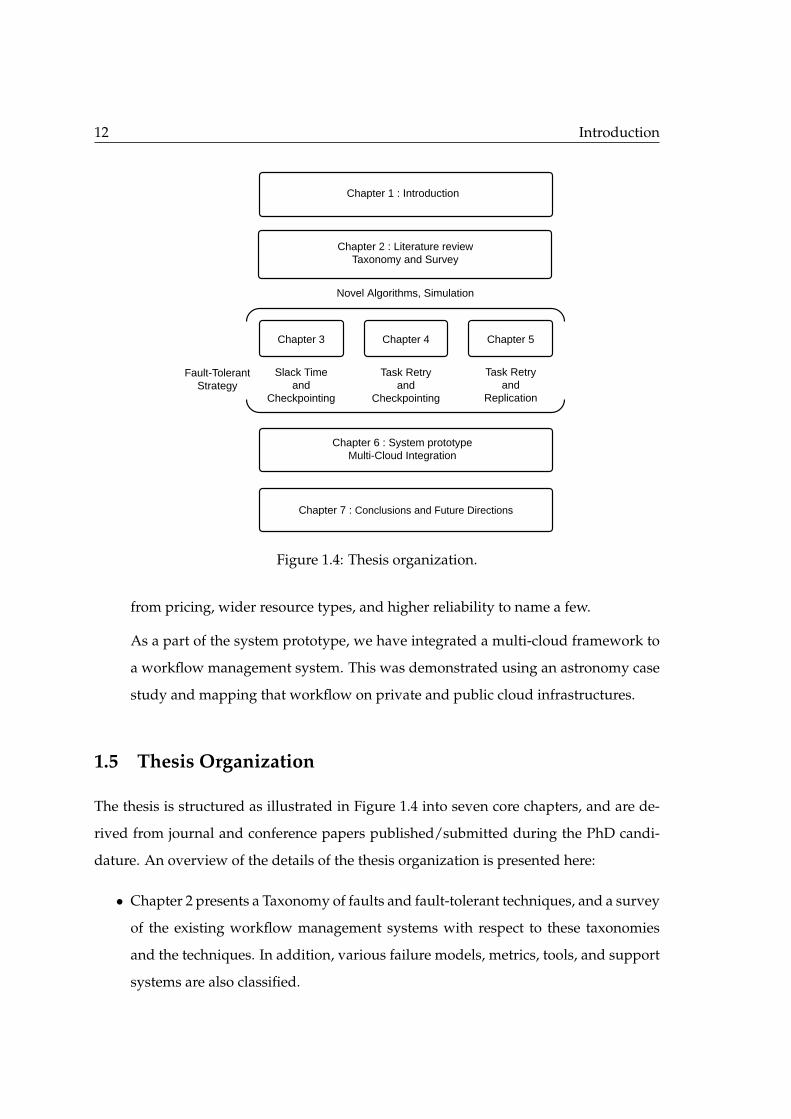
ments . . . . . . . . . . . . . . . . . . . . . . . . . . . . . . . . . . . . . . . . 61.4 Thesis organization. . . . . . . . . . . . . . . . . . . . . . . . . . . . . . . . . 12
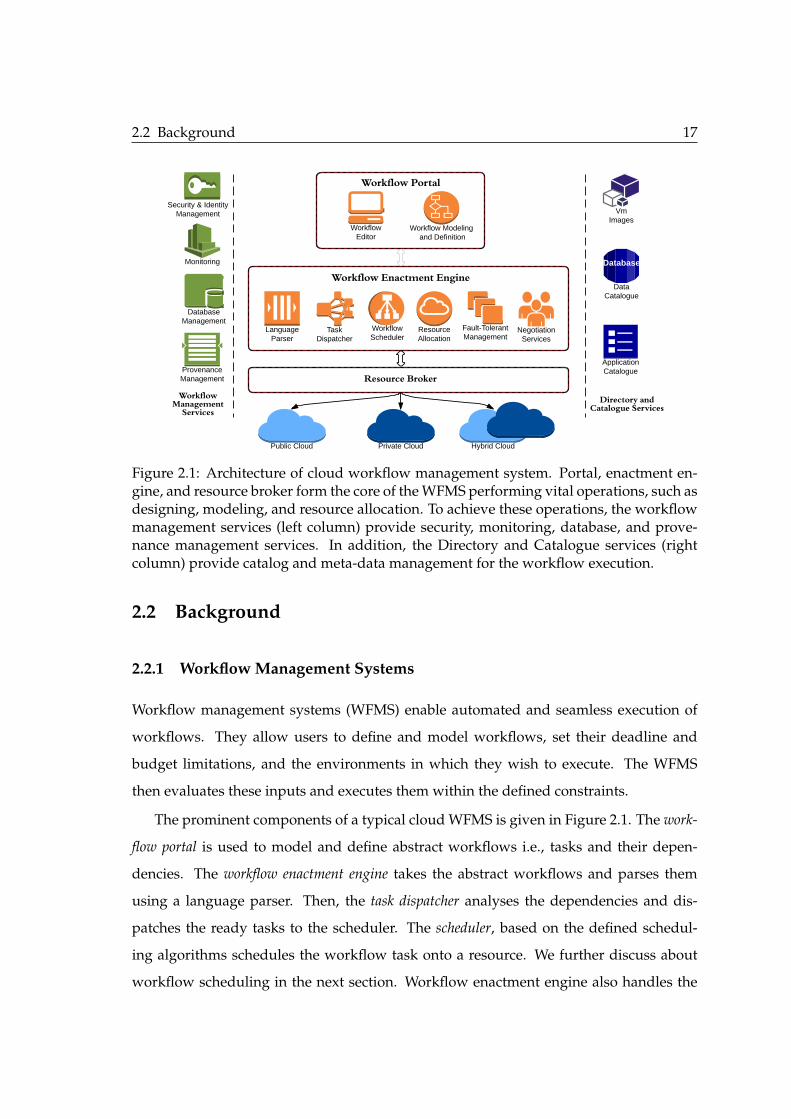
2.1 Architecture of cloud workflow management system. Portal, enactmentengine, and resource broker form the core of the WFMS performing vi-tal operations, such as designing, modeling, and resource allocation. Toachieve these operations, the workflow management services (left column)provide security, monitoring, database, and provenance management ser-vices. In addition, the Directory and Catalogue services (right column)provide catalog and meta-data management for the workflow execution. 17
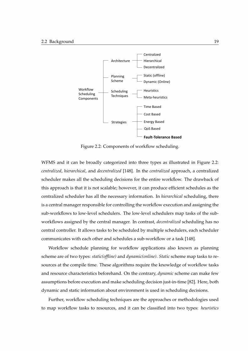
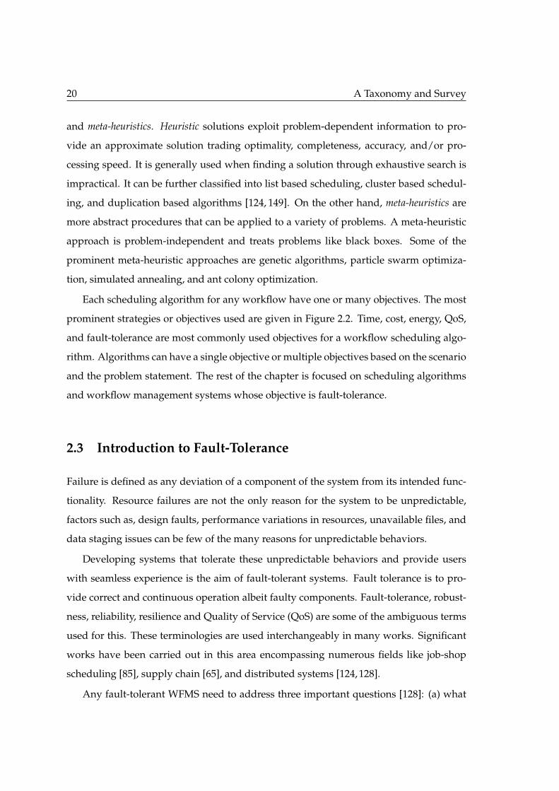
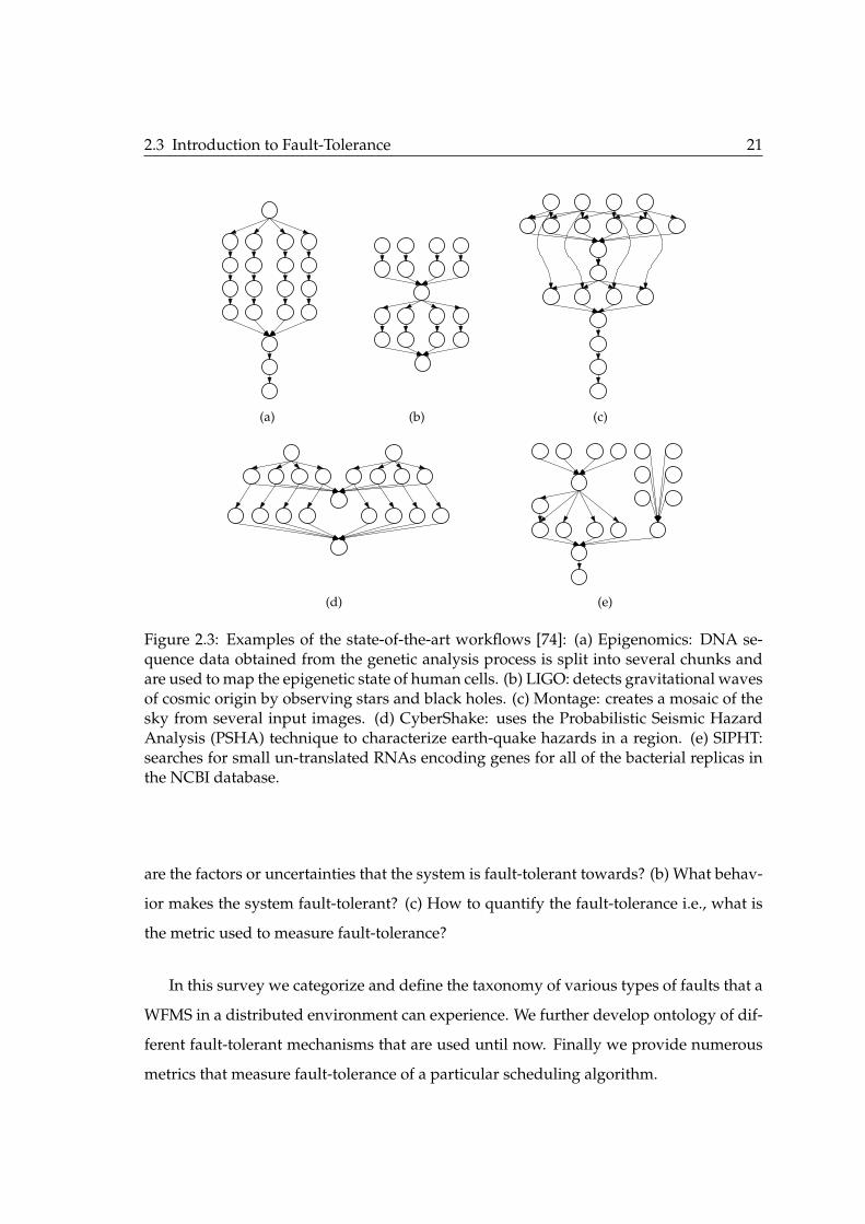
2.2 Components of workflow scheduling. . . . . . . . . . . . . . . . . . . . . . 192.3 Examples of the state-of-the-art workflows [74]: (a) Epigenomics: DNA
sequence data obtained from the genetic analysis process is split into sev-eral chunks and are used to map the epigenetic state of human cells. (b)LIGO: detects gravitational waves of cosmic origin by observing stars andblack holes. (c) Montage: creates a mosaic of the sky from several inputimages. (d) CyberShake: uses the Probabilistic Seismic Hazard Analy-sis (PSHA) technique to characterize earth-quake hazards in a region. (e)SIPHT: searches for small un-translated RNAs encoding genes for all of thebacterial replicas in the NCBI database. . . . . . . . . . . . . . . . . . . . . 21
2.4 Elements through which faults can be characterized. . . . . . . . . . . . . . 232.5 Faults: views and their classifications. . . . . . . . . . . . . . . . . . . . . . 232.6 Taxonomy of workflow scheduling techniques to provide fault-tolerance. 252.7 Different aspects of task duplication technique in providing fault-tolerance. 262.8 Taxonomy of resubmission fault-tolerant technique. . . . . . . . . . . . . . 302.9 Different approaches used in resubmission algorithms. . . . . . . . . . . . 312.10 Classification of resubmission mechanisms. . . . . . . . . . . . . . . . . . . 312.11 Taxonomy of checkpointing mechanism. . . . . . . . . . . . . . . . . . . . . 322.12 Workflow-level checkpointing. . . . . . . . . . . . . . . . . . . . . . . . . . 352.13 Checkpointing schemes. . . . . . . . . . . . . . . . . . . . . . . . . . . . . . 352.14 Forms of provenance. . . . . . . . . . . . . . . . . . . . . . . . . . . . . . . . 372.15 Forms of failure masking. . . . . . . . . . . . . . . . . . . . . . . . . . . . . 37
xvii

2.16 Methods for evaluating trust in trust-based algorithms used for fault-tolerant WFMS. . . . . . . . . . . . . . . . . . . . . . . . . . . . . . . . . . . 40
2.17 Distributions used for modeling failures for workflows in distributed en-vironments. . . . . . . . . . . . . . . . . . . . . . . . . . . . . . . . . . . . . 41
3.1 Effect on robustness with tolerance time Rt . . . . . . . . . . . . . . . . . . 723.2 Effect on makespan for large sized CyberShake and LIGO workflow . . . 723.3 Effect on cost for large sized CyberShake and LIGO workflow . . . . . . . 72
4.1 System architecture. . . . . . . . . . . . . . . . . . . . . . . . . . . . . . . . . 844.2 Generation of bid value through Intelligent Bidding Strategy. . . . . . . . . 884.3 Mean execution cost of algorithms with varying deadline (with 95% confi-
dence interval). . . . . . . . . . . . . . . . . . . . . . . . . . . . . . . . . . . 924.4 Mean execution cost of bidding strategies with varying deadline (with 95%
confidence interval). . . . . . . . . . . . . . . . . . . . . . . . . . . . . . . . 924.5 Mean of task failures due to bidding strategies. . . . . . . . . . . . . . . . . 944.6 Effect of checkpointing on execution cost. . . . . . . . . . . . . . . . . . . . 94
5.1 Figure(a) shows a workflow at time t0, where there is enough slack time.Under such situation the tasks are scheduled onto spot instances. Figure(b)shows a workflow at time t1, where there is no slack time. It also showssome completed tasks. Under such situation, ESCTs are scheduled ontoon-demand instances and replicated on spot instances. Other tasks withslack time are scheduled on spot instances. . . . . . . . . . . . . . . . . . . 102
5.2 Failure probability of algorithms with varying deadline. . . . . . . . . . . 1135.3 Tolerance time of algorithms with varying deadline (with 95% confidence
interval). . . . . . . . . . . . . . . . . . . . . . . . . . . . . . . . . . . . . . . 1135.4 Mean makespan of the proposed algorithms against the baseline with
varying deadlines (with 95% confidence interval). . . . . . . . . . . . . . . 1155.5 Showing the effect of resource consolidation on makespan for ECPTR
heuristic (with 95% confidence interval). . . . . . . . . . . . . . . . . . . . . 1155.6 Mean execution cost of the proposed algorithms against the baseline with
varying deadline (with 95% confidence interval). . . . . . . . . . . . . . . . 1155.7 Replication factor for the algorithms with varying deadline. . . . . . . . . 1155.8 Showing the effect of resource consolidation on cost for ECPTR heuristic
(with 95% confidence interval). . . . . . . . . . . . . . . . . . . . . . . . . . 117
6.1 Cloudbus workflow management system. . . . . . . . . . . . . . . . . . . . 1226.2 Components of workflow scheduling. . . . . . . . . . . . . . . . . . . . . . 1236.3 Apache jclouds system integration architecture. . . . . . . . . . . . . . . . 1276.4 Sequence diagram of jclouds integration. . . . . . . . . . . . . . . . . . . . 1286.5 Class diagram representing resource provisioning through Apache jclouds. 1296.6 Testbed environment setup illustration. . . . . . . . . . . . . . . . . . . . . 1326.7 Montage workflow. . . . . . . . . . . . . . . . . . . . . . . . . . . . . . . . . 1346.8 Effect on makespan under failures. . . . . . . . . . . . . . . . . . . . . . . . 1376.9 Resource instantiation time. . . . . . . . . . . . . . . . . . . . . . . . . . . . 137
xviii

6.10 Output mosaic of the montage workflow. . . . . . . . . . . . . . . . . . . . 138
xix

This page intentionally left blank.
List of Tables
2.1 Features, provenance information and fault-tolerant strategies of work-flow management systems . . . . . . . . . . . . . . . . . . . . . . . . . . . . 45
3.1 Robustness probability Rp of large montage workflow with failure proba-bility model (FP) for different policies. . . . . . . . . . . . . . . . . . . . . . 73
5.1 Spot instance characteristics for US west region (North California AZ) . . 112
6.1 Description of montage workflow tasks . . . . . . . . . . . . . . . . . . . . 133
xxi

This page intentionally left blank.

List of Algorithms
1 FindPCP(t) . . . . . . . . . . . . . . . . . . . . . . . . . . . . . . . . . . . . . . 652 AllocateResource(PCP) . . . . . . . . . . . . . . . . . . . . . . . . . . . . . . 67
3 Schedule(t) . . . . . . . . . . . . . . . . . . . . . . . . . . . . . . . . . . . . . 90
4 FindFreeSlot(t,vms) . . . . . . . . . . . . . . . . . . . . . . . . . . . . . . . . 1055 Schedule(t) . . . . . . . . . . . . . . . . . . . . . . . . . . . . . . . . . . . . . 1075 Schedule(t) - Part Two . . . . . . . . . . . . . . . . . . . . . . . . . . . . . . . 1086 FindSuitableInstances(estimates) . . . . . . . . . . . . . . . . . . . . . . . . . 110
7 FindComputeResource(task) . . . . . . . . . . . . . . . . . . . . . . . . . . . 130
xxiii

This page intentionally left blank.
Chapter 1
Introduction
OVER the last few decades, the experimentation methodology in science has
changed significantly. In particular, tremendous increases in the computational
capacities have enabled deeper and more accurate research within the community. As
scientific research tends to become more complex involving large scale datasets, a scal-
able and automated way to perform these computations and data processing is necessary.
This experimentation typically involves transferring data to a compute node (or compu-
tation to data nodes), running the computations, analysing the results, and managing the
storage of output results. Workflow Management Systems (WFMSs) aim to automate this
entire process, making it easier and more efficient for researchers [41].
A primitive science of workflow design initially emerged within the business world.
They used this concept to automate their business logic and tools. This was later bor-
rowed into the scientific domain. The automation process involves a sequence of tasks
and their dependencies to conduct a business or scientific work. This process is called
workflow orchestration. An instance of a workflow orchestration is called a workflow [41].
That is, workflow is an application composed of a collections of tasks, which are most
frequently executable scripts taking input data and producing output data. These tasks
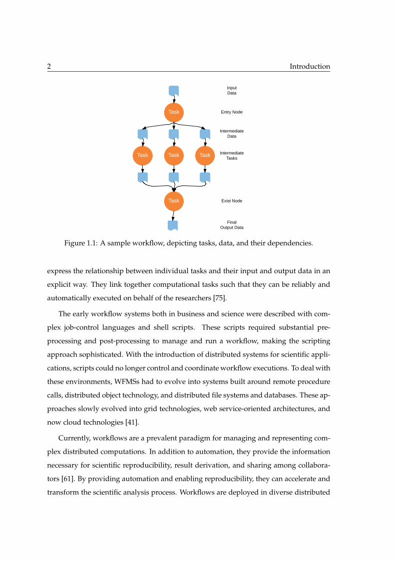
are connected by data and/or control dependencies as illustrated in Figure 1.1. Data de-
pendencies define the flow of data within a workflow application. Normally, when two
tasks are data dependent, then the output of the first task becomes the input of the second
task, and the second task starts its execution after the first task finishes execution, writes
the output data, and stages the data in the location of the second task. Similarly, the con-
trol dependencies define the sequence of executions for the tasks. Therefore, workflows
1
2 Introduction
Task
Task
Task
Task
InputData
Entry Node
Intermediate Data
Intermediate Tasks
Exist Node
Final Output Data
Task
Figure 1.1: A sample workflow, depicting tasks, data, and their dependencies.
express the relationship between individual tasks and their input and output data in an
explicit way. They link together computational tasks such that they can be reliably and
automatically executed on behalf of the researchers [75].
The early workflow systems both in business and science were described with com-
plex job-control languages and shell scripts. These scripts required substantial pre-
processing and post-processing to manage and run a workflow, making the scripting
approach sophisticated. With the introduction of distributed systems for scientific appli-
cations, scripts could no longer control and coordinate workflow executions. To deal with
these environments, WFMSs had to evolve into systems built around remote procedure
calls, distributed object technology, and distributed file systems and databases. These ap-
proaches slowly evolved into grid technologies, web service-oriented architectures, and
now cloud technologies [41].
Currently, workflows are a prevalent paradigm for managing and representing com-
plex distributed computations. In addition to automation, they provide the information
necessary for scientific reproducibility, result derivation, and sharing among collabora-
tors [61]. By providing automation and enabling reproducibility, they can accelerate and
transform the scientific analysis process. Workflows are deployed in diverse distributed
1.1 Introduction to Cloud Computing 3
John McCarthy
"Computing someday may be served as a public utility"
InternetVM
Cloud Data Center Customers
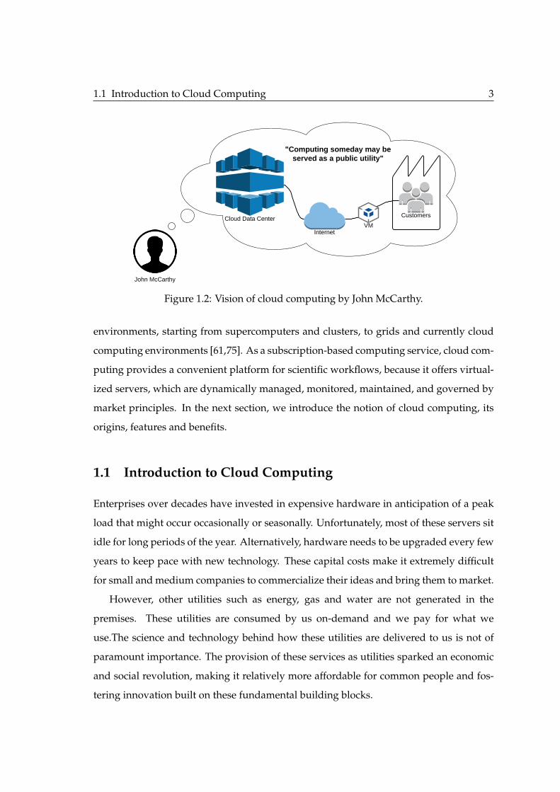
Figure 1.2: Vision of cloud computing by John McCarthy.
environments, starting from supercomputers and clusters, to grids and currently cloud
computing environments [61,75]. As a subscription-based computing service, cloud com-
puting provides a convenient platform for scientific workflows, because it offers virtual-
ized servers, which are dynamically managed, monitored, maintained, and governed by
market principles. In the next section, we introduce the notion of cloud computing, its
origins, features and benefits.
1.1 Introduction to Cloud Computing
Enterprises over decades have invested in expensive hardware in anticipation of a peak
load that might occur occasionally or seasonally. Unfortunately, most of these servers sit
idle for long periods of the year. Alternatively, hardware needs to be upgraded every few
years to keep pace with new technology. These capital costs make it extremely difficult
for small and medium companies to commercialize their ideas and bring them to market.
However, other utilities such as energy, gas and water are not generated in the
premises. These utilities are consumed by us on-demand and we pay for what we
use.The science and technology behind how these utilities are delivered to us is not of
paramount importance. The provision of these services as utilities sparked an economic
and social revolution, making it relatively more affordable for common people and fos-
tering innovation built on these fundamental building blocks.
4 Introduction
In 1960 John McCarthy envisioned (Figure 1.2) that computation someday would be
provided as an utility [115]. Cloud computing is the realization of this vision. With
technologies such as Web Services, Service Oriented Architecture, Web 2.0, Mashups and
Hardware Virtualization becoming popular and widely accepted, they were laying the
path for cloud computing environments.
Cloud computing sprung up as an amalgamation of these technologies. New busi-
ness models centered around it made it an economical option for small and medium
enterprises. Cloud computing is formally defined by NIST (National Institute of Stan-
dards and Technology) as “A model for enabling ubiquitous, convenient, on-demand
network access to a shared pool of configurable computing resources (e.g., networks,
servers, storage, applications, and services) that can be rapidly provisioned and released
with minimal management effort or service provider interaction.” [99].
Cloud computing is subscription-based service that delivers computation as a utility.
The key characteristics of this service that is making it rapidly popular are:
• Delivered on demand: cloud providers paint an illusion of unlimited resources1.
They promise to lease these resources on-demand dynamically as users make re-
quests through easy interfaces and programmable APIs.
• Pay-as-you-go: cloud users pay only for the time they used the resources, much like
other utility services. Cloud providers may have different pricing models, such as,
Amazon charges per hour whereas, Google compute engine charge per minute. But
the user pays for only the approximate period they used the resources.
Cloud computing is highly driven by market principles. Economics drive the cloud
and competition among providers drive the pricing of cloud resources. Cloud com-
puting envisions computing as a commodity and builds business models and ser-
vices around this philosophy.
• Attractive and innovative pricing models: Clouds providers have different pricing
models. As stated earlier, different cloud providers price differently and a single
cloud provider can provision the same resource through multiple pricing models.
1In this thesis, resources, instances and VMs are used interchangeably.

1.2 Research Challenges and Objectives 5
For example, Amazon EC2 instances are provisioned in three main ways: 1) on-
demand instance, where the user pays per hour. 2) spot instances: where a user
bids for the instance and if the bidding price is higher than the spot price then the
instances are leased to the user. And when the bid price fall below spot price, the
instance is terminated. 3) reserved instance, here, the user pays an upfront price
and reserves the instance for a period of time. Further, when they actually use the
instance they pay an additional nominal price for the same.
• Highly elastic: Cloud resources can be leased and shut down when the user pleases.
This gives users flexibility to scale up and down as their application demands.
• Provide different levels of services: Clouds providers provision cloud resources
through various levels of services, such as, 1) infrastructure-as-a-service: where re-
sources like storage, virtual machine, and network are provisioned. 2) platform-as-
a-service: here, a set of tools and services are provided for application development,
deployment and monitoring without worrying about the underlying hardware. 3)
software-as-a-service delivers application over the web to end-users.
• Dynamically configurable: Cloud resources are delivered through the web by eas-
ily manageable graphical interfaces and APIs. They empower cloud providers to
provision services that users can configure dynamically and manage seamlessly.
Because of these features, cloud computing is increasingly used amidst researchers for
scientific workflows to perform high throughput computing and data analysis [89]. Nu-
merous disciplines such as astronomy, physics, biology, and others use scientific work-
flows to perform large scale complex analyses. Features like dynamic provisioning and
innovative pricing models bring a new dimension for workflow scheduling, making it
cost-effective and faster. However, using cloud computing for scheduling scientific work-
flows has some challenges and issues, which are outlined in our next section.
6 Introduction
Workflow Management System
Network Failure
Spot InstanceFailure
Pricing Models
ResourceHeterogeneity
Performance Variationsof Cloud Resources
Resource Failures
Task Failures
WorkflowComplexity
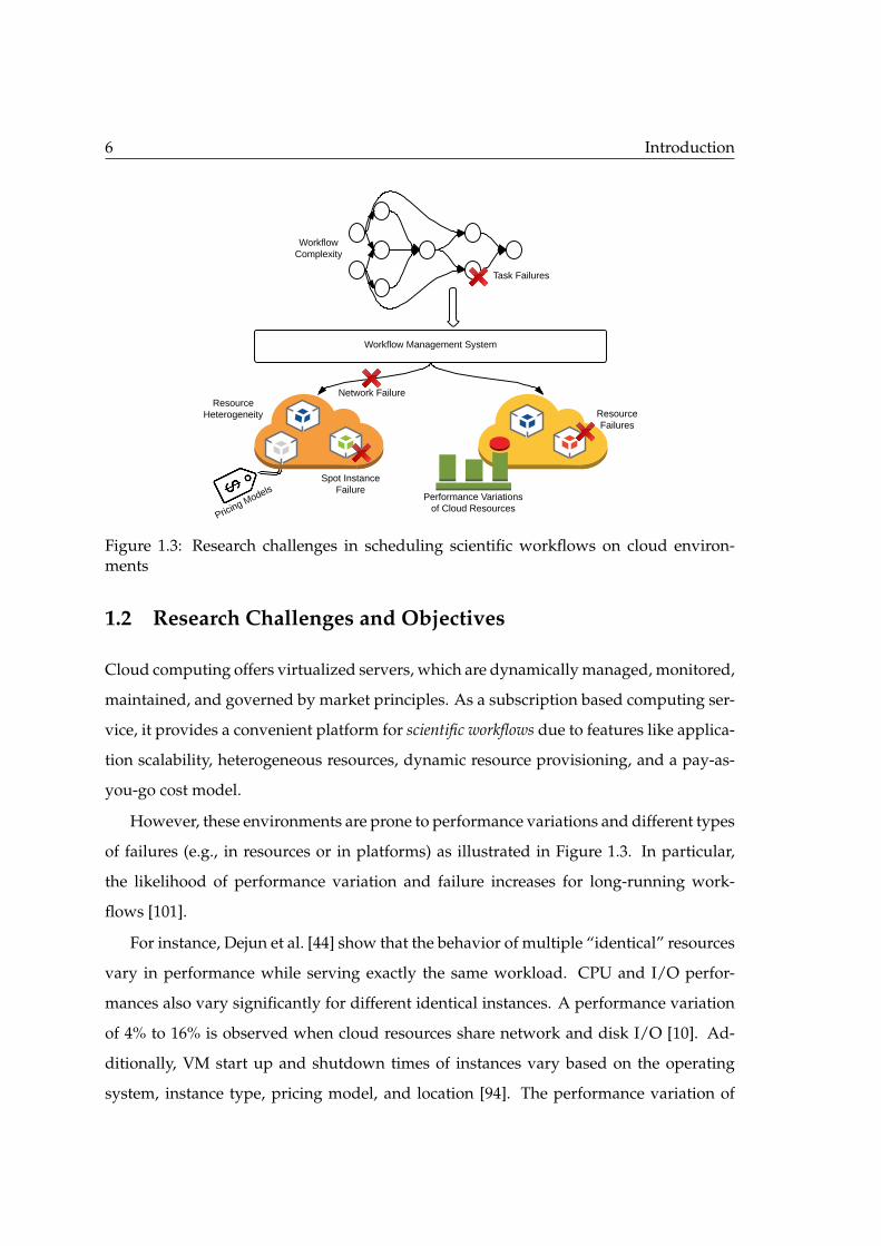
Figure 1.3: Research challenges in scheduling scientific workflows on cloud environ-ments
1.2 Research Challenges and Objectives
Cloud computing offers virtualized servers, which are dynamically managed, monitored,
maintained, and governed by market principles. As a subscription based computing ser-
vice, it provides a convenient platform for scientific workflows due to features like applica-
tion scalability, heterogeneous resources, dynamic resource provisioning, and a pay-as-
you-go cost model.
However, these environments are prone to performance variations and different types
of failures (e.g., in resources or in platforms) as illustrated in Figure 1.3. In particular,
the likelihood of performance variation and failure increases for long-running work-
flows [101].
For instance, Dejun et al. [44] show that the behavior of multiple “identical” resources
vary in performance while serving exactly the same workload. CPU and I/O perfor-
mances also vary significantly for different identical instances. A performance variation
of 4% to 16% is observed when cloud resources share network and disk I/O [10]. Ad-
ditionally, VM start up and shutdown times of instances vary based on the operating
system, instance type, pricing model, and location [94]. The performance variation of
1.2 Research Challenges and Objectives 7
VMs in clouds affects the overall execution time (i.e. makespan) of the workflow. It also
increases the difficulty to estimate the task execution time accurately.
Failures also affect the overall workflow execution time by increasing its makespan.
Failures in a workflow application are mainly of the following types: task failures, ma-
chine (VM) failures, and workflow-level failures [67]. Task failures may occur due to
dynamic execution environment configurations, missing input data, or system errors.
Machine (VM) failures are caused by hardware failures and load in a distributed system,
among other reasons. Workflow level failures can occur due to factors such as machine
failures or cloud outages.
Failures in a workflow environment can occur at different levels [110]: hardware, op-
erating system, middleware, task, workflow, and user. Some of the prominent faults that
occur are network failures, machine crashes, out-of-memory, file not found, authentica-
tion issues, file staging errors, uncaught exceptions, data movement issues, and user-
defined exceptions. Gao et al. [57] identify that cloud systems are not fully protected
systems and are prone to soft errors. Similarly, Ko et al. [80] mention that just in the pe-
riod 2009 to 2011, 172 unique outages occurred among various cloud providers. At the
scale of cloud computing, these errors could potentially worsen application performance.
Added to this, cloud providers like Amazon sell data center capacity that is idle or
unused as spot instances 2 (SI). Users compete in an auction-like market where they bid
a maximum price for these SIs they are willing to pay. The user is provided the instance
whenever the spot price is lower than their bid [136]. However, when the user bid goes
below the spot price, Amazon terminates the resources, such failures are called out-of-bid
failures. Cloud users using SIs to reduce costs must employ strategies to address these
out-of-bid failures [112]. These out-of-bid failures introduce a new dimension to failures,
here failures are proportional to the value of the bid price. These failures are dependent
on the budget an application is willing to spent. Research has shown that these instances
provide huge cost benefits and for that an effective bidding strategy is essential. These
innovative pricing models come with different SLAs that applications need to address.
Cloud resources comes with a variety of configuration characteristics, with different
2http://aws.amazon.com/ec2/purchasing-options/spot-instances/
8 Introduction
cpu cores, memory, storage and others. The execution times of tasks vary on these re-
source, the ability to choose the right resource depending on the deadline and budget of
the workflow is a research challenge. How to address the heterogeneity amidst resources
for an application depending on this deadline and budgetary constraints is a valuable
question that needs to be answered.
Lastly, workflows are generally composed of thousands of tasks, with complicated
dependencies between the tasks. These tasks are interdependent with various execution
times. Scheduling these workflow tasks onto heterogeneous VMs is an NP-Complete
problem [73]. Therefore, necessity for fault-tolerance arises from the complexity of the ap-
plication and environment. Workflows are applications that are most often used in a col-
laborative environment spread across the geography involving various people from dif-
ferent domains (e.g., [74]). So much diversity is a potential cause for adversities. Hence,
to provide a seamless experience over a distributed environment for multiple users of a
complex application, fault-tolerance is a paramount requirement of any WFMS.
This thesis provides effective solutions arising from these research challenges by an-
swering the following fundamental question:
How does one make workflow scheduling algorithms robust and fault-tolerant for cloud
computing environments?
1.3 Methodology
This thesis employs two main methodologies to evaluate the proposed algorithms:
1. Discrete-event simulation: Workflow applications are complex with numerous
jobs and multiple dependencies. Conducting large scale experiments on real cloud
infrastructures is time consuming, costly and extremely difficult. Therefore, a
discrete-event based simulator was employed to evaluate our algorithms. Discrete-
event simulation enables us to conduct experiment and allows us to control var-
ious parameters and evaluate the heuristics under multiple scenarios effectively,
economically, and swiftly. We use and extend CloudSim [21] to simulate the cloud
1.3 Methodology 9
environment. The simulator was extended to support workflow applications, mak-
ing it easy to define, deploy and schedule workflows. A failure event generator was
also integrated into the CloudSim, which generates failures from an input failure
trace.
2. System Prototype: A multi-cloud utility for a workflow management system was
developed. A resource provisioning policy for such an environment was also pro-
posed. The system was tested on two cloud infrastructures to run this experiment:
a private cloud and a public cloud.
1.3.1 Spot Market Traces
This work has used real Amazon AWS EC2 spot market traces for our evaluation of chap-
ter 4 and 5. The spot price history is taken from Amazon EC2 US West region (North Cal-
ifornia availability zone). The spot price history provides information of the spot price
and time for a specific instance.
1.3.2 Failure Traces
For the experiment of Chapter 3, one of the failure models was simulated through fail-
ure traces. Due to lack of publicly available cloud specific failure traces, Condor (CAE)
Grid failure dataset [147], available as a part of Failure Trace Archive [81] was chosen.
This dataset was collected by the Condor team at the University of Wisconsin-Madison
from the Compact Muon Solenoid (CMS) experiment at the European Organization for
Nuclear Research (CERN) [72].
1.3.3 Workflow Applications
State-of-the art workflow applications were used to evaluate the heuristics. Five work-
flows (Montage, CyberShake, Epigenomics, LIGO and SIPHT) were considered. Their
characteristics are explained in detail by Juve et al. [74]. These workflows cover all the
10 Introduction
basic components such as pipeline, data aggregation, data distribution and data redistri-
bution.
1.3.4 Case Study Application
The system prototype was evaluated with the montage application [16], which is a com-
plex astronomy workflow. We have used a montage workflow consisting of 110 tasks,
where the number of the tasks indicate the number of images used. It is an I/O intensive
application, which produces a mosaic of astronomic images.
1.4 Contributions
This thesis proposes novel heuristic algorithms for robust and fault-tolerant workflow
scheduling on cloud computing platforms. Additionally, we use the dynamic pricing
models offered by cloud providers to minimize cost and time whilst providing fault-
tolerant schedules. Specifically, the key findings and contributions of this thesis are:
1 Novel Heuristic Algorithms: Four novel fault-tolerant workflow scheduling
heuristics are proposed in this thesis. These heuristics employ various fault-
tolerant techniques to mitigate failures and performance variations experienced in
the cloud.
– Chapter 3 proposes a heuristic that uses slack time to make schedules robust
against performance variations. The concept of slack time is detailed in Chap-
ters 2 and 3. This algorithm remaps failed tasks and also employs checkpoint-
ing to save execution time.
– Chapter 4 proposes a heuristic that uses both on-demand and spot instances to
save executions cost. It also provides a heuristic that can mitigate spot instance
out-of-bid failures by employing task retry and checkpointing. Results have
shown that using spot instances reduces up to 70% execution costs.
– The heuristic in Chapter 5, similar to the one in chapter 4, uses both on-
demand and spot instances to save execution costs. The proposed heuristics
1.4 Contributions 11
mitigate spot instance out-of-bid failures, additionally it also address VM fail-
ures and network failures by employing task retry and task replication.
– In Chapter 6, a heuristic that utilizes a multi-cloud framework to schedule
resources based on budget constraints is proposed. Upon resource failures,
this algorithms reschedules the failed task onto another resource.
In summary, we have demonstrated numerous heuristic algorithms that employ
fault-tolerant techniques developed specifically for cloud environments, which ad-
dress failures and performance variations experienced in the environment.
2 Bidding Strategy: Bidding strategies are proposed that aid workflow scheduling
algorithms to effectively bid spot instances, such that failures and execution cost
are minimized. The proposed Intelligent Bidding Strategy bids prices closer to the
spot price in the beginning of the execution and gradually increases the bid price
closer to the on-demand price as the workflow nears the completion based on the
current spot price, on-demand price, time flag of the workflow, failure probability
of the previous bid price, and the current time.
3 A performance evaluation study on time, cost and fault-tolerance. Each of the
heuristics proposed are studied with respect to the execution time, cost and fault-
tolerance. Results have demonstrated that our proposed algorithms are robust and
fault-tolerant and can minimize cost and time. We have also studied the effect of
spot price volatility on checkpointing and the results demonstrate that for low spot
prices, frequent checkpointing is not profitable.
4 This thesis also proposes two metrics to measure robustness and fault-tolerance
of a schedule. The first metric robustness probability, measures the likelihood of the
workflow to finish before a given deadline. The second metric tolerance time is the
amount of time a workflow schedule can be delayed, such that the deadline con-
straint is not violated.
5 Multi-cloud resource plug-in: Multiple cloud providers offer clouds resource in an
attractive way. An application running in a multi-cloud environment can benefit
12 Introduction
Chapter 2 : Literature reviewTaxonomy and Survey
Novel Algorithms, Simulation
Chapter 3 Chapter 4 Chapter 5
Slack Timeand
Checkpointing
Task Retryand
Checkpointing
Task Retryand
Replication
Fault-Tolerant Strategy
Chapter 6 : System prototypeMulti-Cloud Integration
Chapter 7 : Conclusions and Future Directions
Chapter 1 : Introduction
Figure 1.4: Thesis organization.
from pricing, wider resource types, and higher reliability to name a few.
As a part of the system prototype, we have integrated a multi-cloud framework to
a workflow management system. This was demonstrated using an astronomy case
study and mapping that workflow on private and public cloud infrastructures.
1.5 Thesis Organization
The thesis is structured as illustrated in Figure 1.4 into seven core chapters, and are de-
rived from journal and conference papers published/submitted during the PhD candi-
dature. An overview of the details of the thesis organization is presented here:
• Chapter 2 presents a Taxonomy of faults and fault-tolerant techniques, and a survey
of the existing workflow management systems with respect to these taxonomies
and the techniques. In addition, various failure models, metrics, tools, and support
systems are also classified.
1.5 Thesis Organization 13
• Chapter 3 proposes a robust scheduling algorithm using checkpointing and slack
time of resources, and resource allocation policies that schedule workflow tasks on
heterogeneous cloud resources while trying to minimize the total elapsed time and
the cost. The chapter is derived from:
– Poola D., Garg S.K., Buyya R., Yang Y., and Ramamohanarao K., Robust
Scheduling of Scientific Workflows with Deadline and Budget Constraints in
clouds, Proceedings of the 28th IEEE International Conference on Advanced
Information Networking and Applications (AINA-2014), Victoria Canada.
• Chapter 4 proposes a scheduling algorithm that schedules tasks on cloud resources
using two different pricing models (spot and on-demand instances) to reduce the
cost of execution whilst meeting the workflow deadline. The proposed algorithm
is fault tolerant against the premature termination of spot instances and also robust
against performance variations of cloud resources. The algorithm proposed uses
task retry and checkpointing techniques to achieve fault-tolerance. The chapter is
derived from:
– Poola D., Ramamohanarao K., and Buyya R., Fault-Tolerant Workflow
Scheduling Using Spot Instances on Clouds, Proceedings of the 13th Interna-
tional Conference on Computational Science (ICCS-2014), Cairns Australia.
• Chapter 5 presents an adaptive, just-in time scheduling algorithm for scientific
workflows. This algorithm judiciously uses both task retry and task replication
to provide fault-tolerance. The proposed scheduling algorithm also consolidates
resources to minimize execution time and cost. The chapter is derived from:
– Poola D., Ramamohanarao K., and Buyya R., Enhancing Reliability of Work-
flow Execution Using Task Replication and Spot Instances, Accepted in the
ACM Transactions on Autonomous and Adaptive Systems (TAAS), ISSN:1556-
4665, ACM Press, New York, USA, 2015 (in press, accepted on Aug. 13, 2015).
• Chapter 6 presents a prototype system developed to provide a multi-cloud integra-
tion to the flagship project of the University of Melbourne, the cloudbus workflow

14 Introduction
management system.
• Chapter 7 concludes this thesis with a summary of contributions, future research
directions, and finals remarks.

Chapter 2
A Taxonomy and Survey
In recent years, workflows have emerged as an important abstraction for collaborative research and
managing complex large-scale distributed data analytics. Workflows are increasingly becoming
prevalent in various distributed environments, such as clusters, grids, and clouds. These envi-
ronments provide complex infrastructures that aid workflows in scaling and parallel execution
of their components. However, they are prone to performance variations and different types of
failures. Thus, workflow management systems need to be robust against performance variations
and tolerant against failures. Numerous research studies have investigated fault-tolerant aspect
of the workflow management system in different distributed systems. In this study, we analyze
these efforts and provide an in-depth taxonomy of them. We present the ontology of faults and
fault-tolerant techniques then position the existing workflow management systems with respect to
the taxonomies and the techniques. In addition, we classify various failure models, metrics, tools,
and support systems. Finally, we identify and discuss the strengths and weaknesses of the cur-
rent techniques and provide recommendations on future directions and open areas for the research
community.
2.1 Introduction
WORKFLOWS orchestrate the relationships between dataflow and computational
components by managing their inputs and outputs. In the recent years, sci-
entific workflows have emerged as a paradigm for managing complex large scale dis-
tributed data analysis and scientific computation. Workflows automate computation,
and thereby accelerate the pace of scientific progress easing the process for researchers.
15
16 A Taxonomy and Survey
In addition to automation, it is also extensively used for scientific reproducibility, result
sharing and scientific collaboration among different individuals or organizations. Scien-
tific workflows are deployed in diverse distributed environments, starting from super-
computers and clusters, to grids and currently cloud computing environments [61, 75].
Distributed environments usually are large scale infrastructures that accelerate com-
plex workflow computation; they also assist in scaling and parallel execution of the work-
flow components. The likelihood of failure increases specially for long-running work-
flows [101]. However, these environments are prone to performance variations and dif-
ferent types of failures. This demands the workflow management systems to be robust
against performance variations and fault-tolerant against faults.
Over the years, many different techniques have evolved to make workflow schedul-
ing fault-tolerant in different computing environments. This chapter aims to catego-
rize and classify different fault-tolerant techniques and provide a broad view of fault-
tolerance in workflow domain for distributed environments.
Workflow scheduling is a well studied research area. Yu et al. [148] provided a com-
prehensive view of workflows, different scheduling approaches, and different workflow
management systems. However, this work did not throw much light on fault-tolerant
techniques in workflows. Plankensteiner et al. [110] have recently studied different fault-
tolerant techniques for grid workflows. Nonetheless, they do not provide a detailed view
into different fault-tolerant strategies and their variants. More importantly, their work
does not encompass other environments like clusters and clouds.
In this chapter, we aim to provide a comprehensive taxonomy of fault-tolerant work-
flow scheduling techniques in different existing distributed environments. We first start
with an introduction to workflows and workflow scheduling. Then, we introduce fault-
tolerance and its necessity. We provide an in-depth ontology of faults in section 2.4. Fol-
lowing which, different fault-tolerant workflow techniques are detailed. In section 2.6,
we describe different approaches used to model failures and also give definition of vari-
ous metrics used in literature to assess fault-tolerance. Finally, prominent workflow man-
agement systems are introduced and a description of relevant tools and support systems
that are available for workflow development is provided.
2.2 Background 17
Task Dispatcher
Fault-Tolerant Management
Resource Allocation
Workflow Enactment Engine
Public Cloud
Cloud
Workflow Editor
Workflow Modeling and Definition
Database Management
Workflow Scheduler
Language Parser
Negotiation Services
Monitoring
Provenance Management
Vm Images
Application Catalogue
Data Catalogue
Database
Workflow Portal
D irectory andCatalogue Services
Workflow M anagement
Services
Resource Broker
Hybrid CloudPrivate Cloud
Security & Identity Management
Figure 2.1: Architecture of cloud workflow management system. Portal, enactment en-gine, and resource broker form the core of the WFMS performing vital operations, such asdesigning, modeling, and resource allocation. To achieve these operations, the workflowmanagement services (left column) provide security, monitoring, database, and prove-nance management services. In addition, the Directory and Catalogue services (rightcolumn) provide catalog and meta-data management for the workflow execution.
2.2 Background
2.2.1 Workflow Management Systems
Workflow management systems (WFMS) enable automated and seamless execution of
workflows. They allow users to define and model workflows, set their deadline and
budget limitations, and the environments in which they wish to execute. The WFMS
then evaluates these inputs and executes them within the defined constraints.
The prominent components of a typical cloud WFMS is given in Figure 2.1. The work-
flow portal is used to model and define abstract workflows i.e., tasks and their depen-
dencies. The workflow enactment engine takes the abstract workflows and parses them
using a language parser. Then, the task dispatcher analyses the dependencies and dis-
patches the ready tasks to the scheduler. The scheduler, based on the defined schedul-
ing algorithms schedules the workflow task onto a resource. We further discuss about
workflow scheduling in the next section. Workflow enactment engine also handles the

18 A Taxonomy and Survey
fault-tolerance of the workflow. It also contains a resource allocation component which
allocates resources to the tasks through the resource broker.
The resource broker interfaces with the infrastructure layer and provides a unified view
to the enactment engine. The resource broker communicates with compute services to
provide the desired resource.
The directory and catalogue services house information about data objects, the applica-
tion and the compute resources. This information is used by the enactment engine, and
the resource broker to make critical decisions.
Workflow management services, in general, provide important services that are essen-
tial for the working of a WFMS. Security and identify services ensure authentication and
secure access to the WFMS. Monitoring tools constantly monitor vital components of the
WFMS and raise alarms at appropriate times. Database management component provides
a reliable storage for intermediate and final data results of the workflows. Provenance
management services capture important information such as, dynamics of control flows
and data, their progressions, execution information, file locations, input and output in-
formation, workflow structure, form, workflow evolution, and system information [141].
Provenance is essential for interpreting data, determining its quality and ownership, pro-
viding reproducible results, optimizing efficiency, troubleshooting and also to provide
fault-tolerance [35, 36].
2.2.2 Workflow Scheduling
As mentioned earlier, a workflow is a collection of tasks connected by control and/or data
dependencies. Workflow structure indicates the temporal relationship between tasks.
Workflows can be represented either in Directed Acyclic Graph (DAG) or non-DAG for-
mats. In this thesis, workflows are represented in DAG formats (as shown in Figure 2.3),
where the vertices represent task nodes and the directed edges represent control and/or
data dependencies.
Scheduling maps workflow tasks on to distributed resources such that the dependen-
cies are not violated. Workflow Scheduling is a well-known NP-Complete problem [73].
The workflow scheduling architecture specifies the placement of the scheduler in a
2.2 Background 19
Workflow SchedulingComponents
PlanningScheme
SchedulingTechniques
Strategies
Architecture
Centralized
Hierarchical
Decentralized
Static (offline)
Dynamic (Online)
Heuristics
Meta-heuristics
Time Based
Cost Based
Energy Based
QoS Based
Fault-Tolerance Based
Figure 2.2: Components of workflow scheduling.
WFMS and it can be broadly categorized into three types as illustrated in Figure 2.2:
centralized, hierarchical, and decentralized [148]. In the centralized approach, a centralized
scheduler makes all the scheduling decisions for the entire workflow. The drawback of
this approach is that it is not scalable; however, it can produce efficient schedules as the
centralized scheduler has all the necessary information. In hierarchical scheduling, there
is a central manager responsible for controlling the workflow execution and assigning the
sub-workflows to low-level schedulers. The low-level schedulers map tasks of the sub-
workflows assigned by the central manager. In contrast, decentralized scheduling has no
central controller. It allows tasks to be scheduled by multiple schedulers, each scheduler
communicates with each other and schedules a sub-workflow or a task [148].
Workflow schedule planning for workflow applications also known as planning
scheme are of two types: static(offline) and dynamic(online). Static scheme map tasks to re-
sources at the compile time. These algorithms require the knowledge of workflow tasks
and resource characteristics beforehand. On the contrary, dynamic scheme can make few
assumptions before execution and make scheduling decision just-in-time [82]. Here, both
dynamic and static information about environment is used in scheduling decisions.
Further, workflow scheduling techniques are the approaches or methodologies used
to map workflow tasks to resources, and it can be classified into two types: heuristics
20 A Taxonomy and Survey
and meta-heuristics. Heuristic solutions exploit problem-dependent information to pro-
vide an approximate solution trading optimality, completeness, accuracy, and/or pro-
cessing speed. It is generally used when finding a solution through exhaustive search is
impractical. It can be further classified into list based scheduling, cluster based schedul-
ing, and duplication based algorithms [124, 149]. On the other hand, meta-heuristics are
more abstract procedures that can be applied to a variety of problems. A meta-heuristic
approach is problem-independent and treats problems like black boxes. Some of the
prominent meta-heuristic approaches are genetic algorithms, particle swarm optimiza-
tion, simulated annealing, and ant colony optimization.
Each scheduling algorithm for any workflow have one or many objectives. The most
prominent strategies or objectives used are given in Figure 2.2. Time, cost, energy, QoS,
and fault-tolerance are most commonly used objectives for a workflow scheduling algo-
rithm. Algorithms can have a single objective or multiple objectives based on the scenario
and the problem statement. The rest of the chapter is focused on scheduling algorithms
and workflow management systems whose objective is fault-tolerance.
2.3 Introduction to Fault-Tolerance
Failure is defined as any deviation of a component of the system from its intended func-
tionality. Resource failures are not the only reason for the system to be unpredictable,
factors such as, design faults, performance variations in resources, unavailable files, and
data staging issues can be few of the many reasons for unpredictable behaviors.
Developing systems that tolerate these unpredictable behaviors and provide users
with seamless experience is the aim of fault-tolerant systems. Fault tolerance is to pro-
vide correct and continuous operation albeit faulty components. Fault-tolerance, robust-
ness, reliability, resilience and Quality of Service (QoS) are some of the ambiguous terms
used for this. These terminologies are used interchangeably in many works. Significant
works have been carried out in this area encompassing numerous fields like job-shop
scheduling [85], supply chain [65], and distributed systems [124, 128].
Any fault-tolerant WFMS need to address three important questions [128]: (a) what
2.3 Introduction to Fault-Tolerance 21
(a) (b) (c)
(d) (e)
Figure 2.3: Examples of the state-of-the-art workflows [74]: (a) Epigenomics: DNA se-quence data obtained from the genetic analysis process is split into several chunks andare used to map the epigenetic state of human cells. (b) LIGO: detects gravitational wavesof cosmic origin by observing stars and black holes. (c) Montage: creates a mosaic of thesky from several input images. (d) CyberShake: uses the Probabilistic Seismic HazardAnalysis (PSHA) technique to characterize earth-quake hazards in a region. (e) SIPHT:searches for small un-translated RNAs encoding genes for all of the bacterial replicas inthe NCBI database.
are the factors or uncertainties that the system is fault-tolerant towards? (b) What behav-
ior makes the system fault-tolerant? (c) How to quantify the fault-tolerance i.e., what is
the metric used to measure fault-tolerance?
In this survey we categorize and define the taxonomy of various types of faults that a
WFMS in a distributed environment can experience. We further develop ontology of dif-
ferent fault-tolerant mechanisms that are used until now. Finally we provide numerous
metrics that measure fault-tolerance of a particular scheduling algorithm.
22 A Taxonomy and Survey
2.3.1 Necessity for Fault-Tolerance in Distributed Systems
Workflows, generally, are composed of thousands of tasks, with complicated dependen-
cies between the tasks. For example, some prominent workflows (as shown in Figure 2.3)
widely considered are Montage, CyberShake, Broadband, Epigenomics, LIGO Inspiral
Analysis, and SIPHT, which are complex scientific workflows from different domains
such as astronomy, life sciences, physics and biology. These workflows are composed of
thousands of tasks with various execution times, which are interdependent.
Workflow tasks are often executed on distributed resources that are heterogeneous
in nature. WFMSs that allocates these workflows uses middleware tools that require to
operate congenially in a distributed environment. This very complex and complicated
nature of WFMSs and its environment invite numerous uncertainties and chances of fail-
ures at various levels.
In particular, in data-intensive workflows that continuously process data, machine
failure is inevitable. Thus, failure is a major concern during the execution of data-
intensive workflows frameworks, such as MapReduce and Dryad [69]. Both transient
(i.e., fail-recovery) and permanent (i.e., fail-stop) failures can occur in data-intensive
workflows [79]. For instance, Google reported on average 5 permanent failures in form
of machine crashes per MapReduce workflow during March 2006 [37] and at least one
disk failure in every run of MapReduce workflow with 4000 tasks.
Necessity for fault-tolerance arises from this very nature of the application and envi-
ronment. Workflows are applications that are most often used in a collaborative environ-
ment are spread across the geography involving various people from different domains
(e.g., [74]). So many diversities are potential causes for adversities. Hence, to provide
a seamless experience over a distributed environment for multiple users of a complex
application, fault-tolerance is a paramount requirement of any WFMS.
2.4 Taxonomy of Faults
Fault is defined as a defect at the lowest level of abstraction. A change in a system state
due to a fault is termed as an error. An error can lead to a failure, which is a deviation
2.4 Taxonomy of Faults 23
of the system from its specified behavior [59, 70]. Before we discuss about fault-tolerant
strategies it is important to understand the fault-detection and identification methodolo-
gies and the taxonomy of faults.
Fault Characteristics
SeverityTimeOriginatorAccuracy Location Stage Frequency
Known Unknown
Faults
Types Classes
Transient Intermittent Permanent Crash Fail-Stop Byzantine
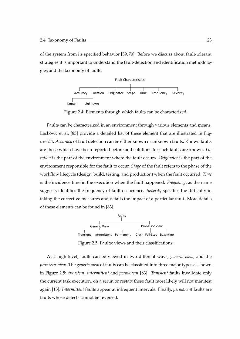
FaultsFigure 2.4: Elements through which faults can be characterized.
Faults can be characterized in an environment through various elements and means.
Lackovic et al. [83] provide a detailed list of these element that are illustrated in Fig-
ure 2.4. Accuracy of fault detection can be either known or unknown faults. Known faults
are those which have been reported before and solutions for such faults are known. Lo-
cation is the part of the environment where the fault occurs. Originator is the part of the
environment responsible for the fault to occur. Stage of the fault refers to the phase of the
workflow lifecycle (design, build, testing, and production) when the fault occurred. Time
is the incidence time in the execution when the fault happened. Frequency, as the name
suggests identifies the frequency of fault occurrence. Severity specifies the difficulty in
taking the corrective measures and details the impact of a particular fault. More details
of these elements can be found in [83].
Fault Characteristics
Severity Time Originator Accuracy Location Stage Frequency
Known Unknown
Generic View Processor View
Transient Intermittent Permanent Crash Fail-Stop
Faults
Byzantine
Figure 2.5: Faults: views and their classifications.
At a high level, faults can be viewed in two different ways, generic view, and the
processor view. The generic view of faults can be classified into three major types as shown
in Figure 2.5: transient, intermittent and permanent [83]. Transient faults invalidate only
the current task execution, on a rerun or restart these fault most likely will not manifest
again [13]. Intermittent faults appear at infrequent intervals. Finally, permanent faults are
faults whose defects cannot be reversed.

24 A Taxonomy and Survey
From a processor’s perspective, faults can be classified into three classes: crash, fail-stop,
and byzantine [59]. This is mostly used for resource or machine failures. In the crash failure
model, the processor stops executing suddenly at a specific point. In fail-stop processors
internal state is assumed to be volatile. The contents are lost when a failure occurs and
it cannot be recovered. However, this class of failure does not perform an erroneous
state change due to a failure [122]. Byzantine faults originate due to random malfunctions
like aging or external damage to the infrastructure. These faults can be traced to any
processor or messages [32].
Faults in a workflow environment can occur at different levels of abstraction [110]:
hardware, operating system, middleware, task, workflow, and user. Some of the promi-
nent faults that occur are network failures, machine crashes, out-of-memory, file not
found, authentication issues, file staging errors, uncaught exceptions, data movement
issues, and user-defined exceptions. Plankensteiner et al. [110] detail various faults and
map them to different level of abstractions.
2.5 Taxonomy of Fault-Tolerant Scheduling Algorithms
This section details the workings of various fault-tolerant techniques used in WFMS. In
the rest of this section, each technique is analyzed and their respective taxonomies are
provided. Additionally, prominent works using each of these techniques are explained.
Figure 2.6 provides an overview of various techniques that are used to provide fault-
tolerance.
2.5.1 Replication
Redundancy in space is one of the widely used mechanisms for providing fault-tolerance.
Redundancy in space means providing additional resources to execute the same task to
provide resilience and it is achieved by duplication or replication of resources. There are
broadly two variants of redundancy of space, namely, task duplication and data replica-
tion.
2.5 Taxonomy of Fault-Tolerant Scheduling Algorithms 25
Taxonomy of Fault-Tolerant Techniques
Provenance
Checkpointing
Resubmission
Replication Rescue Workflow
User-Defined Exception Handling
Alternate Task
Failure Masking
Slack Time
Trust
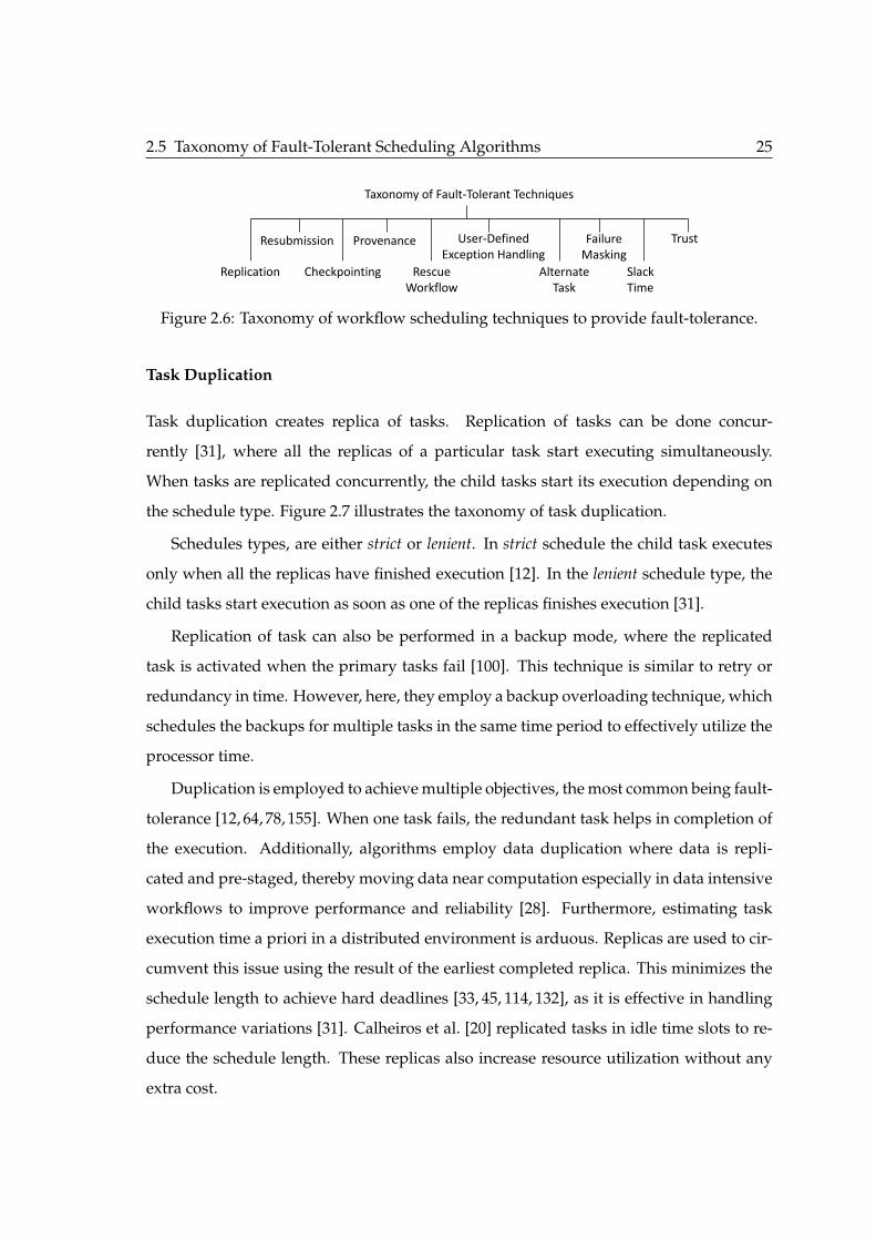
Figure 2.6: Taxonomy of workflow scheduling techniques to provide fault-tolerance.
Task Duplication
Task duplication creates replica of tasks. Replication of tasks can be done concur-
rently [31], where all the replicas of a particular task start executing simultaneously.
When tasks are replicated concurrently, the child tasks start its execution depending on
the schedule type. Figure 2.7 illustrates the taxonomy of task duplication.
Schedules types, are either strict or lenient. In strict schedule the child task executes
only when all the replicas have finished execution [12]. In the lenient schedule type, the
child tasks start execution as soon as one of the replicas finishes execution [31].
Replication of task can also be performed in a backup mode, where the replicated
task is activated when the primary tasks fail [100]. This technique is similar to retry or
redundancy in time. However, here, they employ a backup overloading technique, which
schedules the backups for multiple tasks in the same time period to effectively utilize the
processor time.
Duplication is employed to achieve multiple objectives, the most common being fault-
tolerance [12, 64, 78, 155]. When one task fails, the redundant task helps in completion of
the execution. Additionally, algorithms employ data duplication where data is repli-
cated and pre-staged, thereby moving data near computation especially in data intensive
workflows to improve performance and reliability [28]. Furthermore, estimating task
execution time a priori in a distributed environment is arduous. Replicas are used to cir-
cumvent this issue using the result of the earliest completed replica. This minimizes the
schedule length to achieve hard deadlines [33, 45, 114, 132], as it is effective in handling
performance variations [31]. Calheiros et al. [20] replicated tasks in idle time slots to re-
duce the schedule length. These replicas also increase resource utilization without any
extra cost.

26 A Taxonomy and Survey
Task Duplication
ResourcesTask PlacementObjectiveSchedule
Hybrid
Approach
Exclusive
Resource
Idle
Resource Time
BoundedUnboundedIncrease
Fault-Tolerance
Minimize
Schedule Length
LenientStrict
ApproachResourceResource Time
Figure 2.7: Different aspects of task duplication technique in providing fault-tolerance.
Task duplication is achieved by replicating tasks in either idle cycles of the resources
or exclusively on new resources. Some schedules use a hybrid approach replicating tasks in
both idle cycles and new resources [20]. Idle cycles are those time slots in the resource
usage period where the resources are unused by the application. Schedules that repli-
cate in these idle cycles profile resources to find unused time slot, and replicate tasks in
those slots. This approach achieves benefits of task duplication and simultaneously con-
siders monetary costs. In most cases, however, these idle slots might not be sufficient to
achieve the needed objective. Hence, task duplication algorithms commonly place their
task replicas on new resources. These algorithms trade off resource costs to their objec-
tives.
There is a significant body of work in this area encompassing platforms like clusters,
grids, and clouds [12, 18, 33, 45, 64, 78, 114, 132, 155]. Resources considered can either be
bounded or unbounded depending on the platform and the technique. Algorithms with
bounded resources consider a limited set of resources. Similarly, an unlimited number
of resources are assumed in an unbounded system environment. Resource types used
can either be homogeneous or heterogeneous in nature. homogeneous resources have similar
characteristics, and heterogeneous resources on the contrary vary in their characteristics
such as, processing speed, CPU cores, memory and etc. Darbha et al. [33] is one of the
early works, which presents an enhanced search and duplication based scheduling algo-
rithm (SDBS) that takes into account the variable task execution time. They consider a
distributed system with homogeneous resources and assume an unbounded number of
processors in their system.

2.5 Taxonomy of Fault-Tolerant Scheduling Algorithms 27
Data Replication
Data in workflows are either not replicated (and are stored locally by the processing ma-
chines) or is stored on the distributed file system (DFS) where it is automatically repli-
cated (e.g., in Hadoop Distributed File System (HDFS)). Although the former approach
is efficient, particularly in data-intensive workflows, it is not fault-tolerant. That is, fail-
ure of a server storing data causes the re-execution of the affected tasks. On the other
hand, the latter approach offers more fault tolerance but is not efficient due to significant
network overhead and increasing the execution time of the workflow.
Hadoop, is a platform for executing data-intensive workflows, uses a static replication
strategy for fault-tolerance. That is, users can manually determine the number of replicas
that have to be created from the data. Such static and blind replication approach imposes
a significant storage overhead to the underlying system (e.g., cluster or cloud) and slows
down the execution of the MapReduce workflow. One approach to cope with this prob-
lem is to adjust the replication rate dynamically based on the usage rate of the data. This
will reduce the storage and processing cost of the resources [152]. Cost-effective incre-
mental replication (CIR) [88] is a strategy for cloud based workflows that predicts when
a workflow is needed to replicate to ensure the reliability requirement of the workflow
execution.
There are four major data-replication methods for data-intensive workflows on large-
scale distributed systems (e.g., clouds) namely, synchronous and asynchronous replication,
rack-level replication, and selective replication. These replication methods can be applied
on input, intermediate, or output data of a workflow.
In synchronous data replication, such as those in HDFS, writers (i.e., producer tasks
in a workflow) are blocked until replication finishes. Synchronous replication method
leads to a high consistency because if a writer of block A returns, all the replicas of block
A are guaranteed to be identical and any reader (i.e., consumer tasks in a workflow) of
block A can read any replica. Nonetheless, the drawback of this approach is that the
performance of writers might get affected as they have to be blocked. In contrast, asyn-
chronous data replication [79] allows writers to proceed without waiting for a replication
to complete. The asynchronous data replication consistency is not as accurate as the syn-
28 A Taxonomy and Survey
chronous method because even if a writer of block A returns, a replica of block A may
still be in the replication process. Nonetheless, performance of the writers improves due
to the non-blocking nature. For instance, with an asynchronous replication in Hadoop,
Map and Reduce tasks can proceed without being blocked.
Rack-level data replication method enforces replication of the data blocks on the same
rack in a data center. In cloud data centers, machines are organized in racks with a hi-
erarchical network topology. A two-level architecture with a switch for each rack and
a core switch is a common network architecture in these data centers. In this network
topology the core switch can become bottleneck as it is shared by many racks and ma-
chines. That is, there is heterogeneity in network bandwidth where inter-rack bandwidth
is scarce compared to intra-rack bandwidth. One example of bandwidth bottleneck is
in the Shuffling phase of MapReduce. In this case, as the communication pattern be-
tween machines is all-to-all, the core switches become over-utilized whereas rack-level
switches are underutilized. Rack-level replication reduces the traffic transferred through
the bandwidth-scarce core switch. However, the drawback of the rack-level replication
approach is that it cannot tolerate rack-level failures and if a rack fails, all the replicas
become unavailable. There are observations that show rack-level failures are infrequent
which proves the efficacy of rack-level replication. For instance, one study shows that
Google experiences approximately 20 rack failures within a year [38].
Selective data replication is an approach where the data generated by the previous step
of the workflow are replicated on the machine, where the failed task will be re-executed.
For instance, in a chained MapReduce workflow, once there is a machine failure at the
Map phase, the affected Map tasks can be restarted instantly, if the intermediate data
generated by the previous Reduce tasks were replicated locally on the machine, where
the failed Map task will be re-run. In this manner, the amount of intermediate data that
needs to be replicated in the Map phase is reduced remarkably. However, it is not very
effective for Reduce phase, because Reduce data are mostly locally consumed.
ISS [79] is a system that extends the APIs of HDFS and implements a combination of
three aforementioned replication approaches. It implements a rack-level replication that
asynchronously replicates locally-consumed data. The focus of ISS is on the management

2.5 Taxonomy of Fault-Tolerant Scheduling Algorithms 29
of intermediate data in Hadoop data-intensive workflows. It takes care of all aspects of
managing intermediate data such as writing, reading, Shuffling, and replicating. There-
fore, a programming framework that utilizes ISS does not need to consider Shuffling. ISS
transparently transfers intermediate data from writers (e.g., Map tasks) to readers (e.g.,
Reduce tasks).
As mentioned earlier, replicating input data or intermediate data on stable external
storage systems (e.g., distributed file systems) is expensive for data-intensive workflows.
The overhead is due to data replication, disk I/O, network bandwidth, and serializa-
tion which can potentially dominate the workflow execution time [153]. To avoid these
overheads, in frameworks such as Pregel [93], which is a system for iterative graph com-
putation, intermediate data are maintained in memory. Resilient Distributed Datasets
(RDDs) [153] are distributed memory abstractions that enable data reuse in a fault-
tolerant manner. RDDs are parallel data structures that enable users to persist interme-
diate data in memory and manipulate them using various operators. It also controls the
partitioning of the data to optimize data placement. RDD has been implemented within
the Spark [154] framework.
2.5.2 Resubmission
Resubmission tries to re-execute components to mitigate failures. Resubmission or re-
dundancy in time helps recover from transient faults or soft errors. Resubmission is em-
ployed as an effective fault-tolerant mechanism by around 80% of the WFMSs [110]. Li et
al. [86] claim that 41% of failures are recovered in their work through resubmission. Some
of the WFMS that support resubmission for fault-tolerance are Askalon, Chemomentum,
GWES, Pegasus, P-Grade, Proactive, Triana, Unicore [110].
Resubmission can be classified into two levels: workflow and task resubmission as
illustrated in Figure 2.8. In workflow resubmission, as the name suggests, the entire
application or a partial workflow is resubmitted [15].
Task resubmission, retries the same task to mitigate failure. Task retry/resubmission
can be either done on the same resource or another resource [110]. Resubmission on
the same resource is applicable when a task fails due to a transient failure or due to file

30 A Taxonomy and Survey
Resubmission
WorkflowTask
Arbitrary
Resource
Pre-defined
Resource
Another
Resource
Same
Resource
Reliable
Resource
ReactiveProactive
Resubmission
Mechanism
Hybrid Approach
with Replication
Combined with
Checkpointing
Meta-HeuristicsHeuristics
Resubmission Scheduling Techniques
Figure 2.8: Taxonomy of resubmission fault-tolerant technique.
staging issues. In other cases this might not be the best approach to mitigate failures.
Resubmission of the task can be either done on a fixed predefined resource [67] or on
an arbitrary resource or a resource with high reliability. A fixed predefined resource is
not necessarily the same resource, but the drawbacks are similar to that. Selecting a re-
source arbitrarily without a strategy is not the most effective solution to avoid failures.
Employing a strategy whilst selecting resources, like choosing resources with high relia-
bility, increases the probability of addressing failures. Zhang et al. [155] rank resources
based on a metric called reliability prediction and use this metric to schedule their task
retries.
Resources considered can either be homogeneous or heterogeneous in nature. In a
heterogeneous resource type environment, different resource selection strategies have
different impact on cost and time. A dynamic algorithm must take into consideration
deadline and budget restrictions, and select resources that provide fault-tolerance based
on these constraints. Clouds providers like Amazon, offer resources in an auction-like
mechanism for low cost with low SLAs called spot instances. Poola et al. [112] have
proposed a just-in-time dynamic algorithm that uses these low cost instances to provide
fault-tolerant schedules considering the deadline constraint. They resubmit tasks upon
failures to either spot or on-demand instances based on the criticality of the workflow
deadline. This algorithm is shown to provide fault-tolerant schedule whilst reducing
costs.
Algorithms usually have a predefined limit for the number of retries that they will
attempt [42, 155] to resolve a failure. Some algorithms also have a time interval in addi-
tion to the number of retries threshold [67]. However, there are algorithms that consider
infinite retries as they assume the faults to be transient in nature [26].
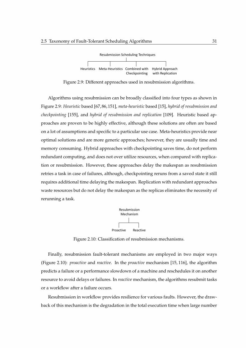
2.5 Taxonomy of Fault-Tolerant Scheduling Algorithms 31
Resubmission
WorkflowTask
Arbitrary
Resource
Pre-defined
Resource
Another
Resource
Same
Resource
Reliable
Resource
ReactiveProactive
Resubmission
Mechanism
Hybrid Approach
with Replication
Combined with
Checkpointing
Meta-HeuristicsHeuristics
Resubmission Scheduling Techniques
Figure 2.9: Different approaches used in resubmission algorithms.
Algorithms using resubmission can be broadly classified into four types as shown in
Figure 2.9: Heuristic based [67,86,151], meta-heuristic based [15], hybrid of resubmission and
checkpointing [155], and hybrid of resubmission and replication [109]. Heuristic based ap-
proaches are proven to be highly effective, although these solutions are often are based
on a lot of assumptions and specific to a particular use case. Meta-heuristics provide near
optimal solutions and are more generic approaches; however, they are usually time and
memory consuming. Hybrid approaches with checkpointing saves time, do not perform
redundant computing, and does not over utilize resources, when compared with replica-
tion or resubmission. However, these approaches delay the makespan as resubmission
retries a task in case of failures, although, checkpointing reruns from a saved state it still
requires additional time delaying the makespan. Replication with redundant approaches
waste resources but do not delay the makespan as the replicas eliminates the necessity of
rerunning a task.
Resubmission
WorkflowTask
Arbitrary
Resource
Pre-defined
Resource
Another
Resource
Same
Resource
Reliable
Resource
ReactiveProactive
Resubmission
Mechanism
Hybrid Approach
with Replication
Combined with
Checkpointing
Meta-HeuristicsHeuristics
Resubmission Scheduling Techniques
Figure 2.10: Classification of resubmission mechanisms.
Finally, resubmission fault-tolerant mechanisms are employed in two major ways
(Figure 2.10): proactive and reactive. In the proactive mechanism [15, 116], the algorithm
predicts a failure or a performance slowdown of a machine and reschedules it on another
resource to avoid delays or failures. In reactive mechanism, the algorithms resubmit tasks
or a workflow after a failure occurs.
Resubmission in workflow provides resilience for various faults. However, the draw-
back of this mechanism is the degradation in the total execution time when large number
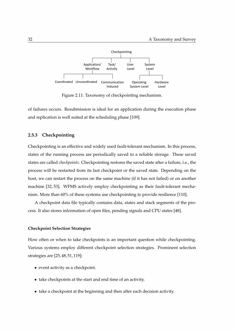
32 A Taxonomy and Survey
Checkpointing
System
Level
User
Level
Task/
Activity
Application/
Workflow
Communication
Induced
UncoordinatedCoordinated Hardware
Level
Operating
System Level
Heavy-WeightLight-Weight
Workflow Level
Checkpointing
Figure 2.11: Taxonomy of checkpointing mechanism.
of failures occurs. Resubmission is ideal for an application during the execution phase
and replication is well suited at the scheduling phase [109].
2.5.3 Checkpointing
Checkpointing is an effective and widely used fault-tolerant mechanism. In this process,
states of the running process are periodically saved to a reliable storage. These saved
states are called checkpoints. Checkpointing restores the saved state after a failure, i.e., the
process will be restarted from its last checkpoint or the saved state. Depending on the
host, we can restart the process on the same machine (if it has not failed) or on another
machine [32, 53]. WFMS actively employ checkpointing as their fault-tolerant mecha-
nism. More than 60% of these systems use checkpointing to provide resilience [110].
A checkpoint data file typically contains data, states and stack segments of the pro-
cess. It also stores information of open files, pending signals and CPU states [48].
Checkpoint Selection Strategies
How often or when to take checkpoints is an important question while checkpointing.
Various systems employ different checkpoint selection strategies. Prominent selection
strategies are [25, 48, 51, 119]:
• event activity as a checkpoint.
• take checkpoints at the start and end time of an activity.
• take a checkpoint at the beginning and then after each decision activity.
2.5 Taxonomy of Fault-Tolerant Scheduling Algorithms 33
• user defines some static stages during build-stage.
• take checkpoint when runtime completion duration is greater than maximum ac-
tivity duration.
• take checkpoint when runtime completion duration is greater than mean duration
of the activity.
• when an activity fails.
• when an important activity finishes completion.
• after a user defined deadline (e.g., percentage of workflow completion).
• underlying system changes like availability of services.
• application defined stages.
• based on linguistic constructs for intervention of programmers.
Issues and Challenges
Checkpointing provides fault-tolerance against transient faults only. If there is a design
fault, checkpointing cannot help recover from it [49]. Another challenge here is to decide
the number of checkpoints to be taken. As the frequency of checkpoints increases, the
overhead also increases, whereas lower checkpoints leads to excessive loss of computa-
tion [134]. The overhead imposed by checkpointing depends on the level that it is applied
(e.g., process or virtual machine level). A mathematical model is provided in [118] to cal-
culate the checkpointing overhead of virtual machines.
In message-passing systems inter-process dependencies are introduced by messages.
When one or more processes fail, these dependencies may lead to a restart even if the
processes did not fail. This is called rollback propagation that may lead the system to
the initial state. This situation is called domino effect [51]. Domino effect occurs if check-
points are taken independently in an uncoordinated fashion in a system. This can be
avoided by performing checkpoints in a coordinated manner. Further, if checkpoints are
taken to maintain system-wide consistency then domino effect can be avoided [51].

34 A Taxonomy and Survey
Taxonomy of Checkpointing
As shown in Figure 2.11, there are four major checkpointing approaches:
Application/workflow-level, task/activity level, user level, and system level implementa-
tion.
In application/workflow-level checkpointing implementation is usually performed
within the source code, or is automatically injected into the code using external tools.
It captures the state of the entire workflow and its intermediate data [48, 134]. This can
be further classified into coordinated, uncoordinated, or communication-induced [51]. Coor-
dinated approach takes checkpoints in a synchronized fashion to maintain a global state.
Recovery in this approach is simple and domino effect is not experienced in this method.
It maintains only one permanent checkpoint on a reliable storage, eliminating the need
for garbage collection. The drawback is incurring a large latency in committing the out-
put [51].
Coordinated checkpointing can further be achieved in the following ways: Non-
blocking Checkpoint Coordination, Checkpointing with Synchronized Clocks, Checkpointing
and Communication Reliability, and Minimal Checkpoint Coordination.
Non-Blocking Checkpoint Coordination: Here, the initiator takes a checkpoint and broad-
casts a checkpoint request to all other activities. Each activity or task takes a checkpoint
once it receives this checkpoint request and then further re-broadcasts the request to all
tasks/activities.
Checkpointing with Synchronized Clocks: This approach is done with loosely synchro-
nized clocks that trigger local checkpointing for all activities without an initiator.
Checkpointing and Communication Reliability: This protocol saves all the in-transit mes-
sages by their destination tasks. These messages need not be saved when communication
channels are assumed to be unreliable.
Minimal Checkpoint Coordination: In this case, only a minimum subset of the tasks/ac-
tivities is saved as checkpoints. The initiator identifies all activities with which it has
communicated since the last checkpoint and sends them a request. Upon receiving the
request, each activity further identifies other activities it has communicated since the last
checkpoint and sends them a request.
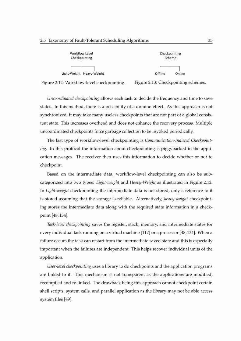
2.5 Taxonomy of Fault-Tolerant Scheduling Algorithms 35
Checkpointing
System
Level
User
Level
Task/
Activity
Application/
Workflow
Communication
Induced
UncoordinatedCoordinated Hardware
Level
Operating
System Level
Heavy-WeightLight-Weight
Workflow Level
Checkpointing
Figure 2.12: Workflow-level checkpointing.
Flat Hierarchical
Failure Masking
Online Offline
Checkpointing Scheme
Figure 2.13: Checkpointing schemes.
Uncoordinated checkpointing allows each task to decide the frequency and time to save
states. In this method, there is a possibility of a domino effect. As this approach is not
synchronized, it may take many useless checkpoints that are not part of a global consis-
tent state. This increases overhead and does not enhance the recovery process. Multiple
uncoordinated checkpoints force garbage collection to be invoked periodically.
The last type of workflow-level checkpointing is Communication-Induced Checkpoint-
ing. In this protocol the information about checkpointing is piggybacked in the appli-
cation messages. The receiver then uses this information to decide whether or not to
checkpoint.
Based on the intermediate data, workflow-level checkpointing can also be sub-
categorized into two types: Light-weight and Heavy-Weight as illustrated in Figure 2.12.
In Light-weight checkpointing the intermediate data is not stored, only a reference to it
is stored assuming that the storage is reliable. Alternatively, heavy-weight checkpoint-
ing stores the intermediate data along with the required state information in a check-
point [48, 134].
Task-level checkpointing saves the register, stack, memory, and intermediate states for
every individual task running on a virtual machine [117] or a processor [48,134]. When a
failure occurs the task can restart from the intermediate saved state and this is especially
important when the failures are independent. This helps recover individual units of the
application.
User-level checkpointing uses a library to do checkpoints and the application programs
are linked to it. This mechanism is not transparent as the applications are modified,
recompiled and re-linked. The drawback being this approach cannot checkpoint certain
shell scripts, system calls, and parallel application as the library may not be able access
system files [49].

36 A Taxonomy and Survey
System-level checkpointing can be done either at the operating system level or the hardware
level. This mechanism is transparent to the user and it does not necessarily modify the
application program code. The problem with operating system level checkpointing is
that it cannot be portable and modification at the kernel level is not always possible and
difficult to achieve [49].
Performance Optimization
As discussed earlier, optimizing performance in a checkpoint operation is a challenge.
The frequency of checkpoints impacts the storage and computation load. Checkpointing
schemes can be broadly divided into online and offline checkpointing schemes as illus-
trated in Figure 2.13.
An offline checkpointing scheme determines the frequency for a task before its exe-
cution. The drawback being it is not an adaptive approach. On the other hand, online
schemes determine the checkpointing interval dynamically based on the frequency of
fault occurrences and the workflow deadline. Dynamic checkpointing is more adaptive
and is able to optimize performance of the WFMS.
Checkpointing in WFMS
WFMSs employ checkpointing at various levels. At Workflow-level, two types of check-
pointing can be employed Light-weight and Heavy-weight as stated earlier. Light-weight
checkpointing is used by Chemomentum, GWEE, GWES, Pegasus, P-grade, and Traina
WFMS. Similarly, heavy-weight checkpointing is employed by GWEE and GWES. Task-
level checkpointing is employed by both Pegasus and P-Grade. Proactive WFMS check-
points at the operating system level [110].
Kepler also checkpoints at the workflow layer [101], whereas, Karajan allows check-
pointing the current state of the workflow at a global level. Here, timed or program-
directed checkpoints can be taken, or checkpoints can be taken automatically at precon-
figured time intervals, or it can be taken manually [139]. SwinDeW-C checkpoints using
a minimum time redundancy based selection strategy [91].

2.5 Taxonomy of Fault-Tolerant Scheduling Algorithms 37
2.5.4 Provenance
Provenance is defined as the process of metadata management. It describes the origins
of data, the processes involved in its production, and the transformations it has under-
gone. Provenance can be associated with process(es) that aid data creation [127]. Prove-
nance captures multiple important information like dynamics of control and data flows,
their progressions, execution information, file locations, input and output information,
workflow structure, form, workflow evolution, and system information [141]. Prove-
nance is essential for interpreting data, determining its quality and ownership, providing
reproducible results, optimizing efficiency, troubleshooting, and also to provide fault-
tolerance [35, 36].
RetrospectiveProspective
Provenance
Failure Models Distributions
Log-NormalWeibullExponentialPoisson UniformLog-NormalWeibullExponentialPoisson Uniform
Figure 2.14: Forms of provenance.
Flat Hierarchical
Failure Masking
Online Offline
Checkpointing Scheme
Figure 2.15: Forms of failure masking.
As detailed in Figure 2.14, provenance can be of two forms: prospective and retrospec-
tive [36]. Prospective provenance captures the specifications that need to be followed to
generate a data product or class of data products. Retrospective provenance captures the
executed steps similar to a detailed log of task execution. It also captures information
about the execution environment used to derive a specific data product.
Provenance information is used to rerun workflows, these reruns can overcome tran-
sient system errors [126]. Provenance allows users to trace state transitions and detect the
cause of inconsistencies. It is used to design recovery or undo paths from workflow fault
states at the task granularity level. It is used as an effective tool to provide fault-tolerance
in several WFMS.
2.5.5 Rescue Workflow
The rescue workflow technique ignores failed tasks and executes the rest of the workflow
until no more forward progress can be made.
A rescue workflow description called rescue DAG containing statistical information
38 A Taxonomy and Survey
of the failed nodes is generated, which is used for later resubmission [148]. Rescue work-
flow technique is used by Askalon, Kepler and DAGMan [91, 148].
2.5.6 User-Defined Exception Handling
In this fault-tolerant technique, users can specify a particular action or a predefined so-
lution for certain task failures in a workflow. Such a technique is called user-defined
exception handling [148]. This could also be used to define alternate tasks for predefined
type of failures [67].
This mechanism is employed by Karajan, GWES, Proactive, and Kepler among the
prominent WFMS [91, 110].
2.5.7 Alternate Task
The alternate task fault-tolerant scheduling technique defines an alternative implemen-
tation of a particular task. When the predefined task fails, its alternative implementation
is used for execution. This technique is particularly useful when two or more different
implementations are available for a task. Each implementation has different execution
characteristics but take the same input and produce same outputs. For example, there
could be a task with two implementations, where one is less memory or compute inten-
sive but unreliable, while the alternate implementation is memory intensive or compute
intensive but more reliable. In such cases, the later implementation can be used as an
alternative task.
This technique is also useful to semantically undo the effect of a failed task, that is,
alternate tasks can be used to clean up the states and data of a partially executed failed
task [67, 148].
2.5.8 Failure Masking
Failure masking fault-tolerant technique ensures service availability, despite failures in
tasks or resources [49]. This is typically achieved by redundancy, and in the event of
2.5 Taxonomy of Fault-Tolerant Scheduling Algorithms 39
failure the services are provided by the active (i.e., surviving) tasks or resources masking
failures. Masking can be of two forms: hierarchical group masking and flat group masking.
Hierarchical group masking uses a coordinator to monitor the redundant components
and decides which copy should replace the failed component. The major drawback of
this approach is the single point of failure of the coordinator.
Flat group masking resolves this single point of failure by being symmetric. That is, the
redundant components are transparent and a voting process is used to select the replace-
ment in adversity. This approach does not have a single point of failure, but imposes
more overhead to the system.
2.5.9 Slack Time
Task slack time represents a time window within which the task can be delayed without
extending the makespan. It is intuitively related to the robustness of the schedule. Slack
time is computed as the minimum spare time on any path from the considered node to
the exit node of the workflow. The formal definition of slack is given by Sakellariou and
Zhao in [116].
Shi et al. [124] present a robust scheduling for heterogeneous resources using slack
time to schedule tasks. They present a ε-constraint method where robustness is an ob-
jective and deadline is a constraint. This scheduling algorithm tries to find schedules
with maximum slack time without exceeding the specified deadline. Similarly, Poola et
al. [111] presented a heuristic considering heterogeneous cloud resources, they divided
the workflow into partial critical paths, and based on the deadline and budget added
slack time to these partial critical path’s estimated execution time. Slack time added to
the schedule enables the schedule time to tolerate performance variations and failures up
to a certain extent, without violating the deadline.
2.5.10 Trust-Based Scheduling Algorithms
Distributed environments have uncertainties and are unreliable, added to this, some
service providers may slightly violate SLAs (with respect to performance, startup or
shutdown times) for many reasons including profitability. Therefore, WFMS typically
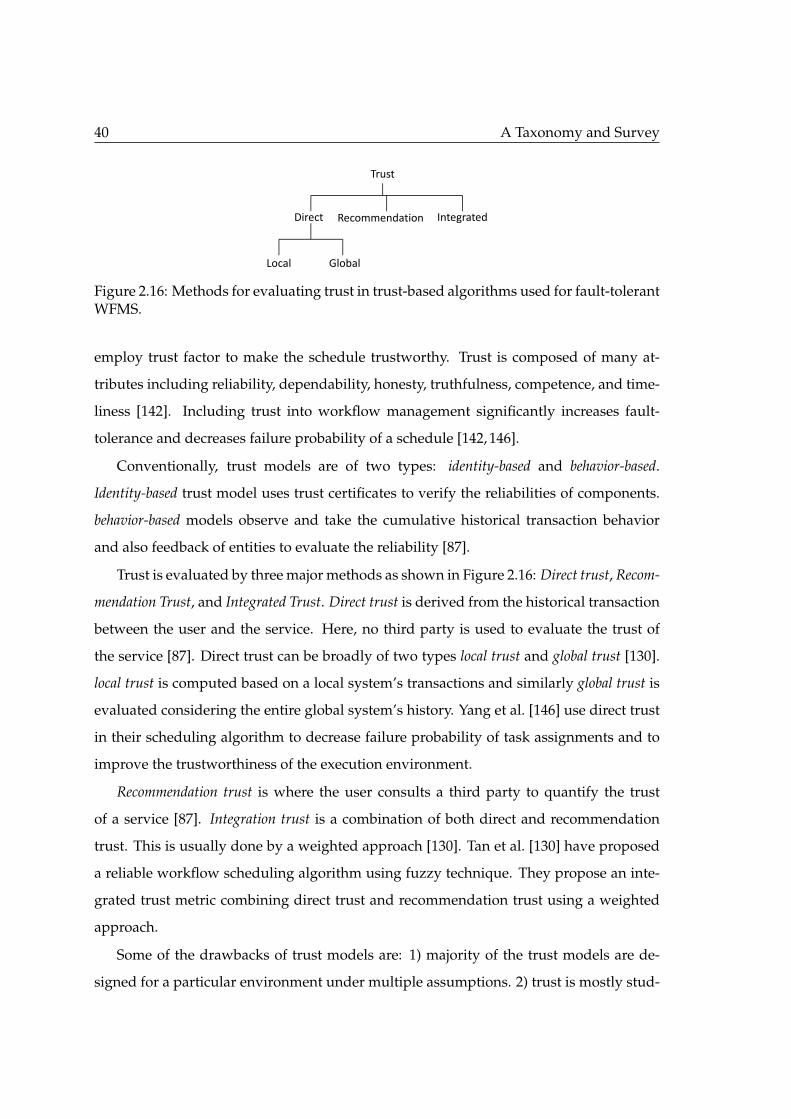
40 A Taxonomy and Survey
Trust
IntegratedRecommendationDirect
GlobalLocal
Figure 2.16: Methods for evaluating trust in trust-based algorithms used for fault-tolerantWFMS.
employ trust factor to make the schedule trustworthy. Trust is composed of many at-
tributes including reliability, dependability, honesty, truthfulness, competence, and time-
liness [142]. Including trust into workflow management significantly increases fault-
tolerance and decreases failure probability of a schedule [142, 146].
Conventionally, trust models are of two types: identity-based and behavior-based.
Identity-based trust model uses trust certificates to verify the reliabilities of components.
behavior-based models observe and take the cumulative historical transaction behavior
and also feedback of entities to evaluate the reliability [87].
Trust is evaluated by three major methods as shown in Figure 2.16: Direct trust, Recom-
mendation Trust, and Integrated Trust. Direct trust is derived from the historical transaction
between the user and the service. Here, no third party is used to evaluate the trust of
the service [87]. Direct trust can be broadly of two types local trust and global trust [130].
local trust is computed based on a local system’s transactions and similarly global trust is
evaluated considering the entire global system’s history. Yang et al. [146] use direct trust
in their scheduling algorithm to decrease failure probability of task assignments and to
improve the trustworthiness of the execution environment.
Recommendation trust is where the user consults a third party to quantify the trust
of a service [87]. Integration trust is a combination of both direct and recommendation
trust. This is usually done by a weighted approach [130]. Tan et al. [130] have proposed
a reliable workflow scheduling algorithm using fuzzy technique. They propose an inte-
grated trust metric combining direct trust and recommendation trust using a weighted
approach.
Some of the drawbacks of trust models are: 1) majority of the trust models are de-
signed for a particular environment under multiple assumptions. 2) trust is mostly stud-
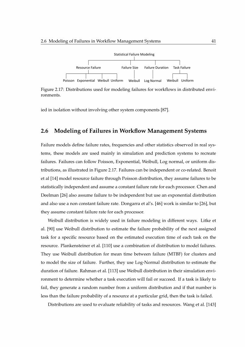
2.6 Modeling of Failures in Workflow Management Systems 41
Statistical Failure Modeling
Failure Size Failure Duration Task Failure Resource Failure
Poisson Exponential Weibull Uniform Weibull Uniform Weibull Log Normal
Figure 2.17: Distributions used for modeling failures for workflows in distributed envi-ronments.
ied in isolation without involving other system components [87].
2.6 Modeling of Failures in Workflow Management Systems
Failure models define failure rates, frequencies and other statistics observed in real sys-
tems, these models are used mainly in simulation and prediction systems to recreate
failures. Failures can follow Poisson, Exponential, Weibull, Log normal, or uniform dis-
tributions, as illustrated in Figure 2.17. Failures can be independent or co-related. Benoit
et al [14] model resource failure through Poisson distribution, they assume failures to be
statistically independent and assume a constant failure rate for each processor. Chen and
Deelman [26] also assume failure to be independent but use an exponential distribution
and also use a non constant failure rate. Dongarra et al’s. [46] work is similar to [26], but
they assume constant failure rate for each processor.
Weibull distribution is widely used in failure modeling in different ways. Litke et
al. [90] use Weibull distribution to estimate the failure probability of the next assigned
task for a specific resource based on the estimated execution time of each task on the
resource. Plankensteiner et al. [110] use a combination of distribution to model failures.
They use Weibull distribution for mean time between failure (MTBF) for clusters and
to model the size of failure. Further, they use Log-Normal distribution to estimate the
duration of failure. Rahman et al. [113] use Weibull distribution in their simulation envi-
ronment to determine whether a task execution will fail or succeed. If a task is likely to
fail, they generate a random number from a uniform distribution and if that number is
less than the failure probability of a resource at a particular grid, then the task is failed.
Distributions are used to evaluate reliability of tasks and resources. Wang et al. [143]
42 A Taxonomy and Survey
uses exponential distribution to evaluate task reliability based on real-time reputation.
The reputation is defined by using their task failure rate.
All the above works consider failures to be independent. However, Javadi et al. [70]
consider failures to be spatial and temporally correlated. Spatial correlations of failures
imply that multiple failures occur on various nodes with a specified time interval. Tem-
poral correlation denotes skewness in failures over time. They use spherical covariance
model to determine temporal failure correlation and Weibull distribution for failure mod-
eling.
2.7 Metrics Used to Quantify Fault-Tolerance
There are various metrics to measure the robustness or fault-tolerance of a workflow
schedule. Each metric measures a different aspect and reports the schedule robustness
based on certain constraints and assumptions. We present some prominent metrics used
in the literature. The makespan considered in most cases is the actual makespan and not
the predicted makespan.
Makespan Standard Deviation: It reports the standard deviation of the makespan.
Narrower the distribution, better the schedule [23].
Makespan differential Entropy: Measures the differential entropy of the distribution,
if the uncertainty is less, then the schedule is more robust [17].
Mean slack: Amount of time the task can be delayed without delaying the schedule
is called task slack time. The slack of a schedule is the summation of slack times of all the
tasks. Hence, more the slack in a schedule means more failures it can tolerate. Therefore,
the schedule is more robust [17].
Probabilistic metric: Defines the makespan probability within two bounds. If the
probability is high, then the robustness is high. This is because higher probability indi-
cates that the makespan is close to the average makespan [123].
Lateness likelihood: A schedule is late if the makespan exceeds a given deadline.
This metric gives the probability of the schedule to be late. If the lateness likelihood is
high, the robustness of the schedule is low [124].

2.7 Metrics Used to Quantify Fault-Tolerance 43
Reliability: Reliability of a compute service during a given time is defined as per the
equation 2.1,
Reliability = (1− (numFailure/n)) ∗mtt f , (2.1)
where, numFailure is the number of failures experiences by the users, n is the number of
users, and mtt f is the promised mean time to failure [58].
Workflow Failure Ratio: It is the percentage of failed workflows due to one or more
task failures [6].
Request Rejection Ratio: It is the ratio of number of rejected requests to the total
requests [6].
Workflow Success Probability: The success probability of the entire workflow is
given as a product of the success probabilities of individual tasks [155].
Standard Length Ratio: It indicates the performance of the workflow. It is the ratio
of turnaround time to the critical path time including the communication time between
tasks. Turnaround time is the workflows’ running time. Lower value of this metric sig-
nifies better performance [155].
Trust: This metric presents the trustworthiness of a particular resource. It is given by
the following equation
Trust(Si) = wi ∗ DT(Si) + (1− wi) ∗ RT(Si), (2.2)
where, DT(Si) is the direct trust based on historical experiences of the ith service, RT(Si)
is the recommendation trust by other users and wi is the weight of DT(Si) and RT(Si) for
the ith service [130].
Failure probability (Rp): It is the likelihood of the workflow to finish before the given
deadline [111, 124], which can be formulated as below:
Rp = (TotalRun− FailedRun)/(TotalRun), (2.3)
where TotalRun is number of times the experiment was conducted and FailedRun is
number of times the constraint, f inishtn 6 D was violated. Here, D is the deadline of
the workflow and f inishtn is the workflow elapsed time.

44 A Taxonomy and Survey
Tolerance time (Rt): It is the amount of time a workflow can be delayed without vi-
olating the deadline constraint. This provides an intuitive measurement of robustness
given the same schedule and resource to task mapping, expressing the amount of uncer-
tainties it can further withstand. It is given by the Equation 2.4
Rt = D− f inishtn . (2.4)
2.8 Survey of Workflow Management Systems and Frameworks
This section provides a detailed view of the state-of-the-art WFMSs and also provide
information about the different fault-tolerant techniques used, as described in section 2.5.
These WFMSs are summarized in Table 2.1.
2.8.1 Askalon
Askalon [53] is a WFMS developed at the University of Innsbruck, Austria. It facil-
itates the development and optimization of applications on grid computing environ-
ments [53, 148]. The system architecture consists of the following components: 1) Sched-
uler: maps single or multiple workflows tasks onto the grid; 2)Enactment Engine: ensures
reliable and fault-tolerant execution of applications; 3)Resource Manager: is responsible
for negotiation, reservation, allocation of resources and automatic deployment of ser-
vices. It also shields the user from low-level grid middleware technology; 4) Performance
Analysis: supports automatic instrumentation and bottleneck detection (e.g., excessive
synchronization, communication, load imbalance, inefficiency, or non scalability) within
the grid; 5) Performance Prediction service: estimates execution times of workflow activi-
ties through a training phase and statistical methods based on a combination of historical
data obtained from the training phase and analytical models [53, 54].
Askalon uses an xml-based workflow language called AGWL for workflow orchestra-
tion. It can be used to specify DAG-constructs, parallel loops and conditional statements
such as switch and if/then/else. AGWL can express sequence, parallelism choice and

2.8 Survey of Workflow Management Systems and Frameworks 45Ta
ble
2.1:
Feat
ures
,pro
vena
nce
info
rmat
ion
and
faul
t-to
lera
ntst
rate
gies
ofw
orkfl
owm
anag
emen
tsys
tem
s
WFM
SFe
atur
esPr
oven
ance
Faul
t-to
lera
ntSt
rate
gy
Ask
alon
Uni
vers
ity
ofIn
nsbr
uck
,Aus
tria
.http://www.dps.uibk.ac.at/
projects/askalon/
•Se
rvic
eO
rien
ted
Arc
hite
ctur
e•
Sing
leA
cces
sU
ser
Port
al•
UM
LW
orkfl
owEd
itor
•X
509
cert
ifica
tes
supp
ort
•A
maz
onEC
2A
PIsu
ppor
t•
Gri
dsan
dcl
ouds
N/A
Res
ubm
issi
on,
repl
icat
ion,
chec
kpoi
ntin
g/re
star
t,m
i-gr
atio
n,us
er-d
efine
dex
cept
ion,
resc
uew
orkfl
ow.
Pega
sus
USC
Info
rmat
ion
Scie
nces
Inst
itut
ean
dth
eU
nive
rsit
yof
Wis
cons
inM
adis
on.
http://pegasus.isi.edu/
•Po
rtab
ility
/R
euse
•Pe
rfor
man
cean
dre
liabi
lity
•Sc
alab
ility
•Pr
oven
ance
•D
ata
Man
agem
ent
•D
eskt
ops,
clus
ters
,gri
ds,a
ndcl
ouds
Kee
pstr
ack
ofda
talo
ca-
tion
s,da
tare
sult
s,an
dso
ft-
war
eus
edw
ith
its
para
me-
ters
.
Task
Res
ubm
issi
on,
Wor
kflow
Res
ubm
issi
on,
wor
kflow
-lev
elch
eckp
oint
ing,
alte
rnat
ive
data
sour
ces,
resc
uew
orkfl
ow.
Tria
naC
ardi
ffU
nive
rsit
y,U
nite
dK
ingd
om.
•M
odul
arja
vaw
orkfl
owen
viro
nmen
t•
Job
queu
ing
•C
ompr
ehen
sive
tool
box
libra
ries
•G
rids
and
clou
ds
N/A
Ligh
t-w
eigh
tch
eckp
oint
ing
and
rest
art
ofse
rvic
esar
esu
ppor
ted
atth
ew
orkfl
owle
vel.
Res
ubm
issi
ons
are
supp
orte
dat
the
task
leve
lby
the
wor
kflow
engi
ne,a
ndal
tern
ate
task
tech
niqu
eis
also
empl
oyed
.
Uni
core
6C
olla
bora
tion
betw
een
Ger
man
rese
arch
inst
i-tu
tion
san
din
dust
ries
.
•Su
ppor
tfor
virt
ualo
rgan
izat
ions
,X.5
09ce
rtifi
-ca
tes
•Im
prov
edda
tam
anag
emen
tth
roug
hD
ataF
inde
r•
Supp
orts
fore
ach
loop
san
dit
erat
ion
over
file-
sets
•G
rids
and
clus
ter
N/A
Res
ubm
issi
onan
dre
liabi
lity
mea
sure
men
tof
task
and
wor
kflow
sar
esu
ppor
ted.
Kep
lar
UC
Dav
is,
UC
Sant
aBa
rbar
a,an
dU
CSa
nD
iego
.https://kepler-project.org/
•In
depe
nden
tly
Exte
nsib
le,
Rel
iabl
e,op
enan
da
com
preh
ensi
vesy
stem
•Su
ppor
tsm
ulti
-dis
cipl
inar
yap
plic
atio
ns•
Gri
ds,c
lust
ers,
and
clou
ds
Dat
aan
dpr
oces
spr
ove-
nanc
ein
form
atio
nis
reco
rded
.
Res
ubm
issi
ons,
chec
kpoi
ntin
g,al
tern
ativ
eve
rsio
ns,
erro
r-st
ate
and
user
-defi
ned
exce
ptio
nha
ndlin
gm
ech-
anis
ms
toad
dres
sis
sues
are
empl
oyed
.
Clo
udbu
sW
FEn
gine
The
Uni
vers
ity
ofM
elbo
urne
,Aus
tral
ia.
http://cloudbus.org/workflow/
•Ea
syto
use
Gra
phic
aled
itor
•U
ser-
frie
ndly
port
alfo
rdi
scov
ery,
mon
itor
ing
and
sche
dulin
g•
Gri
ds,c
lust
ers,
and
clou
ds
Prov
enan
cein
form
atio
nof
data
isre
cord
ed.
Failu
rear
eha
ndle
dby
resu
bmit
ting
the
task
sto
re-
sour
ces.
Tave
rna
Cre
ated
byth
em
yGri
dte
am.
•C
apab
leof
perf
orm
ing
iter
atio
nsan
dlo
opin
g•
Supp
orts
data
stre
amin
g•
Gri
ds,c
lust
ers,
and
clou
ds
Prov
enan
cesu
ite
reco
rds
serv
ice
invo
cati
ons
and
wor
kflow
resu
lts
both
inte
rmed
iate
and
final
.
Res
ubm
issi
onan
dal
tern
ate
reso
urce
s.
e-Sc
ienc
eC
entr
alN
ewca
stle
Uni
vers
ity,
Uni
ted
Kin
gdom
.http://www.esciencecentral.co.uk/
•Ea
syan
def
ficie
ntac
cess
thro
ugh
web
brow
ser
•Pr
ovid
esA
PIs
for
exte
rnal
appl
icat
ions
•A
llda
taar
eve
rsio
ned
•Pr
ivat
ean
dpu
blic
clou
ds
e-SC
prov
enan
cese
rvic
eco
llect
sin
form
atio
nre
gard
-in
gal
lsys
tem
even
ts.
Prov
ides
fine
grai
ned
secu
rity
cont
rolm
odel
edar
ound
grou
psan
dus
er-t
o-us
erco
nnec
tion
s.
Swin
DeW
-CSw
inbu
rne
Uni
vers
ity
ofTe
chno
logy
,A
us-
tral
ia.
•C
loud
base
dpe
er-t
o-pe
erW
FMS
•W
ebpo
rtal
allo
ws
user
sto
acce
ssen
tire
WFM
S•
Clo
uds
data
prov
enan
ceis
reco
rded
duri
ngw
ork-
flow
exec
utio
n
Che
ckpo
inti
ngis
empl
oyed
.Q
oSm
anag
emen
tco
m-
pone
nts
incl
udes
perf
orm
ance
man
agem
ent,
data
man
-ag
emen
tand
secu
rity
man
agem
ent.
46 A Taxonomy and Survey
iteration workflow structures. Askalon uses a graphical interface called Teuta to sup-
port the graphical specification of grid workflow applications based on the UML activity
diagram [53, 54].
Askalon can detect faults at the following levels. 1) Hardware level: Machine crashes
and network failures. 2) OS level: Exceeded disk quota, out of disk space, and file not
found errors. 3) Middleware-level: Failed authentication, failed job-submission, unreach-
able services and file staging failures. 4) Workflow level: Unavailable input data, data
movement faults. However, the system cannot detect task level faults such as memory
leak, uncaught exception, deadlock/livelock, incorrect output data, missing shared li-
braries, and job crashes. Further, the system can recover from the following faults at
different levels: 1) Hardware level: Machine crashes and network failures; 2) OS level:
Exceeded disk quota, out of disk space; 3) Middleware-level: Failed job-submission; 4)
Workflow level: Data movement faults. Nonetheless, it does not recover from task level
faults and user-defined exceptions. Fault-tolerant techniques like checkpointing, migra-
tion, restart, retry and replication are employed to recover from these faults [53, 54, 110].
2.8.2 Pegasus
It is a project of the USC Information Sciences Institute and the Computer Science de-
partment at the University of Wisconsin Madison, United States. Pegasus enables sci-
entists to construct workflows in abstract terms by automatically mapping the high-level
workflow descriptions onto distributed infrastructures (e.g., Condor, Globus, or Amazon
EC2). Multiple workflow applications can be executed in this WFMS [3].
Workflows can be described using DAX, a DAG XML description. The abstract work-
flow describes application components and their dependencies in the form of a DAG [42].
Workflow application can be executed in variety of target platforms including local
machine, clusters, grids and clouds. The WFMS executes jobs, manages data, monitors
execution and handles failures. Pegasus WFMS has five major components: 1) Mapper,
generates an executable workflow from an abstract workflow. It also restructures the
workflow to maximize performance. It further adds transformations aiding in data man-
agement and provenance generation; 2) Local Execution Engine, submits jobs to the local
2.8 Survey of Workflow Management Systems and Frameworks 47
scheduling queue by managing dependencies and changing the state; 3) Job Scheduler,
schedules and manages individual jobs on local and remote resources; 4) Remote Execu-
tion Engine, manages execution of one or more tasks on one or more remote nodes; 5)
Monitoring Component, monitors the workflow execution. It records the tasks logs, per-
formance and provenance information in a workflow database. It notifies events such as
failures, success and statuses [43].
Pegasus stores and queries information about the environment, such as storage sys-
tems, compute nodes, data location, through various catalogs. Pegasus discovers log-
ical files using the Replica Catalog. It looks up various user executables and binaries
in Transformation Catalog. Site Catalog is used to locate computational and storage re-
sources [42, 43].
Pegasus has its own lightweight job monitoring service called Kickstart. The map-
per embeds all jobs with Kickstart [43]. This helps in getting runtime provenance and
performance information of the job. This information is further used for monitoring the
application.
Resource selection is done using the knowledge of available resources, their char-
acteristics and the location of the input data. Pegasus supports pluggable components
where a customized approach for site selection can be performed. It has few choices of
selection algorithms, such as random, round-robin and min-min.
Pegasus can handle failures dynamically at various levels building on the features of
DAGMan and HTCondor. It is equipped to detect and recover from faults. It can de-
tect faults at the following levels: At the Hardware and Operating System levels, it can
detect exceeding CPU time limit and file non-existence. At the level of Middleware, it de-
tects authentication, file staging, and job submission faults. At Task and Workflow levels
job crashes and input unavailability are detected. DAGMan helps recover the following
failures at different levels: at Hardware level, it can recover from machine crashes and
network failures by automatically resubmitting. Middleware faults detected can also be
recovered. Data movement faults can also be treated with recovery at task and work-
flow level. At Workflow level, redundancy is used and light-weight checkpoints are sup-
ported [43,110]. If a job fails more than the set number of retries, then the job is marked as
48 A Taxonomy and Survey
a fatal failure. When a workflow fails due to such failures, the DAGMan writes a rescue
workflow. The rescue workflow is similar to the original DAG without the fatal failure
nodes. This workflow will start from the point of failure. Users can also re-plan the work-
flow, in case of workflow failures and move the computation left to an alternate resource.
Pegasus uses retries, resubmissions, and checkpointing to achieve fault-tolerance [43].
Monitoring and debugging is also done to equip users to track and monitor their
workflows. Three different logs are generated which are used to collect and process
data [43]. 1) Pegasus Mapper Log helps relate the information about the abstract work-
flow from the executable workflow allowing users to correlate user-provided tasks to the
jobs created by Pegasus. 2) Local workflow execution engine logs contain status of each
job of the workflow. 3) Job logs capture provenance information about each job. It con-
tains fine-grained execution statistics for each task. It also includes a web dashboard to
facilitate monitoring [43].
2.8.3 Triana
Triana [133] is a data-flow system developed at Cardiff University, United Kingdom. It is
a combination of an intuitive graphical interface with data analysis tools. It aims to sup-
port applications on multiple environments, such as peer-to-peer and grid computing.
Triana allows users to integrate their own middleware and services besides providing a
vast library of pre-written tools. These tools can be used in a drag-and-drop fashion to
orchestrate a workflow.
Triana addresses fault-tolerance in a user-driven and interactive manner. When faults
occur, the workflow is halted, displaying a warning, and allowing the user to rectify.
At the hardware level, machine crashes and network errors are detected. Missing files
and most other faults can be detected by the workflow engine at the operating system
level. With the exception of deadlock and memory leaks that cannot be detected at the
middleware and the task level, all other faults can be detected. In the workflow level, data
movement and input availability errors are detected. Light-weight checkpointing and
restart of services are supported at the workflow level. Retries, alternate task creations,
and restarts are supported at the task level by the workflow engine [110].
2.8 Survey of Workflow Management Systems and Frameworks 49
2.8.4 UNICORE 6
Unicore [129] is a European grid technology developed by collaboration between German
research institutions and industries. Its main objective is to access distributed resources
in a seamless, secure, and intuitive way. The architecture of UNICORE is divided into
three layers namely, client layer, service layer, and systems layer. In the client layer, various
clients, like UNICORE Rich Client (graphical interface), UNICORE command-line (UCC)
interface, and High Level API (HiLA) a programming API are available.
The service layer contains all the vital services and components. This layers has ser-
vices to maintain a single site or multiple sites. Finally, the system layer has the Tar-
get System Interface (TSI) between the UNICORE and the low-level resources. Recently
added functionalities to UNICORE 6 contains support for virtual organizations, interac-
tive access based on X.509 certificates using Shibboleth, and improved data management
through the integration of DataFinder. GridBeans and JavaGAT help users to support
their applications further. UNICORE 6 also introduces for-each-loops and iteration over
file-sets in addition to existing workflow constructs. It also supports resubmission and
reliability measurement for task and workflows. Added to these new monitoring tools,
availability and service functionality are also improved.
2.8.5 Kepler
The Kepler system [8, 92, 101] is developed and maintained by the cross-project collabo-
ration consisting of several key institutions: UC Davis, UC Santa Barbara, and UC San
Diego. Kepler system allows scientists to exchange, archive, version, and execute their
workflows.
Kepler is built on Ptolemy, a dataflow-oriented system. It focuses on an actor-oriented
modeling with multiple component interaction semantics. Kepler can perform both static
and dynamic checking on workflow and data. Scientists can prototype workflows before
the actual implementation. Kepler system provides web service extensions to instantiate
any workflow operation. Their grid service enables scientists to use grid resources over
the internet for a distributed workflow. It further supports foreign language interfaces via
50 A Taxonomy and Survey
the Java Native Interface (JNI), giving users the benefits to use existing code and tools.
Through Kepler users can link semantically compatible but syntactically incompatible
services together (using XSLT, Xquery, etc.). Kepler supports heterogeneous data and
file formats through Ecological Metadata Language (EML) ingestion. Fault-tolerance is
employed through retries, checkpointing, and alternative versions.
2.8.6 Cloudbus Workflow Management System
The WFMS [19, 107, 108] developed at The University of Melbourne provides an efficient
management technique for distributed resources. It aids users by enabling their appli-
cations to be represented as a workflow and then execute them on the cloud platform
from a higher level of abstraction. The WFMS is equipped with an easy-to-use graphical
workflow editor for application composition and modification, an XML-based workflow
language for structured representation. It further includes a user-friendly portal with
discovery, monitoring, and scheduling components.
Workflow monitor of the WFMS enables users to view the status of each task, they can
also view the resource and the site where the task is executed. It also provides the failure
history of each task. The workflow engine contains workflow language parser, resource
discovery, dispatcher, data management, and scheduler. Tuple space model, event-driven
approach, and subscription approach make WFMS flexible and loosely coupled in design,
as they allow task managers to be independent allowing their communication through
events [150]. Failures are handled by resubmitting the tasks to resources without a failure
history for such tasks. WFMS uses either Aneka [137] and/or Broker [138] to manage
applications running on distributed resources.
2.8.7 Taverna
Taverna [103,144] is an open source and domain-independent WFMS created by the my-
Grid team. It is a suite of tools used to design and execute scientific workflows and aid
in silico experimentation. Taverna engine is capable of performing iterations, looping,
and data streaming. It can interact with various types of services including web services,
2.8 Survey of Workflow Management Systems and Frameworks 51
data warehouses, grid services, cloud services, and various scripts like R, distributed
command-line, or local scripts.
The Taverna server allows workflows to be executed in distributed infrastructures
like clusters, grids and clouds. The server has an interface called Taverna Player through
which users can execute workflows from web browsers or through third-party clients.
Taverna Provenance suite records service invocations and workflow results both interme-
diate and final. It also supports pluggable architecture that facilitates extensions and
contributions to the core functionalities. Here, retries and alternate resources are used to
mitigate failures.
2.8.8 The e-Science Central (e-SC)
The e-Science Central [66] was created in 2008 as a cloud data processing system for
e-Science projects. It can be deployed on both private and public clouds. Scientists can
upload data, edit, run workflows, and share results using a Web Browser. It also provides
an application programming interface through which external application can use the
platforms functionality.
The e-SC facilitates data storage management, tools for data analysis, automation
tools, and also controlled data sharing. All data are versioned and support reproduction
of experiments, aiding investigation into data changes, and their analysis.
The e-SC provenance service collects information regarding all system events and this
provenance data model is based on the Open Provenance Model (OPM) standard. It also
provides fine grained security control modeled around groups and user-to-user connec-
tions.
2.8.9 SwinDeW-C
Swinburne Decentralized Workflow for cloud (SwinDew-C) [91] is a cloud based peer-
to-peer WFMS developed at Swinburne University of Technology, Australia. It is devel-
oped based on their earlier project for grid called SwinDeW-G. It is built on SwinCloud
infrastructure that offers unified computing and storage resources. The architecture of
52 A Taxonomy and Survey
SwinDeW-C can be mapped into four basic layers: application layer, platform layer, unified
resource layer, and fabric layer.
In SwinDeW-C users should provide workflow specification consisting of task defini-
tions, process structures, and QoS constraints. SwinDeW-C supports two types of peers:
An ordinary SwinDeW-C peer is a cloud service node with software service deployed on
a virtual machine; and SwinDeW-C coordinator peers, are special nodes with QoS, data,
and security management components. The cloud workflow specification is submitted
to any coordinated peer, which will evaluate the QoS requirement and determine its ac-
ceptance through a negotiation process. A coordinated peer is setup within every service
provider. It also has pricing and auditing components. All peers that reside in a service
provider communicate with its coordinated peer for resource provisioning. Here, each
task is executed by a SwinDeW-C peer during the run-time stage.
SwinDeW-C also allows virtual machines to be created with public clouds providers,
such as Amazon, Google, and Microsoft. Checkpointing is employed for providing relia-
bility. Additionally, QoS management components including performance management,
data management, and security management are integrated into the coordinated peers.
2.8.10 Big Data Frameworks: MapReduce, Hadoop, and Spark
Recently, big data analytics has gained considerable attention both in academia and in-
dustry. Big data analytics is heavily reliant on tools developed for such analytics. In fact,
these tools implement a specific form of workflows, known as MapReduce [39].
MapReduce framework is a runtime system for processing big data workflows. The
framework usually runs on a dedicated platform (e.g., a cluster). There are currently two
major implementations of the MapReduce framework. The original implementation with
a proprietary license was developed by Google [39]. After that, Hadoop framework [84]
was developed as an open-source product by Yahoo! and widely applied for big data
processing.
The MapReduce framework is based on two main input functions, Map and Reduce
that are implemented by the programmer. Each of these functions is executed in parallel
on large-scale data across the available computational resources. Map and Reduce collec-
2.8 Survey of Workflow Management Systems and Frameworks 53
tively form a usually huge workflow to process large datasets. The MapReduce storage
functionality for storing input, intermediate, and output data is supported by distributed
file systems developed specifically for this framework, such as Hadoop Distributed File
System (HDFS) [125] and Google File System (GFS) [60].
More specifically, every MapReduce program is composed of three subsequent phases
namely, Map, Shuffle, and Reduce. In the Map phase, the Map function implemented by
the user is executed on the input data across the computational resources. The input data
is partitioned into chunks and stored in a distributed file system (e.g., HDFS). Each Map
task loads some chunks of data from the distributed file system and produces intermedi-
ate data that are stored locally on the worker machines. Then, the intermediate data are
fed into the Reduce phase. That is, the intermediate data are partitioned to some chunks
and processed by the Reduce function, in parallel.
Distributing the intermediate data across computational resources for parallel Reduce
processing is called Shuffling. The distribution of intermediate data is accomplished in
an all-to-all manner that imposes a communication overhead and often is the bottleneck.
Once the intermediate data are distributed, the user-defined Reduce function is executed
and the output of the MapReduce is produced. It is also possible to have a chain of
MapReduce workflows (a.k.a multi-stage MapReduce), such as Yahoo! WebMap [7]. In
these workflows, the output of a MapReduce workflow is the intermediate data for the
next MapReduce workflow.
Spark [154] is a framework developed at UC Berkeley and is being utilized for re-
search and production applications. Spark offers a general-purpose programming inter-
face in the Scala programming language [102] for interactive and in-memory data mining
across clusters with large datasets. Spark has proven to be faster than Hadoop for itera-
tive applications.
MapReduce has been designed to tolerate faults that commonly occur at large scale
infrastructures where there are thousands of computers and hundreds of other devices
such as network switches, routers, and power units. Google and Hadoop MapReduce
can tolerate crashes of Map and Reduce tasks. If one of these tasks stops, it is detected
and a new instance of the same task is launched. In addition, data are stored along with
54 A Taxonomy and Survey
their checksum on disks that enables corruption detection. MapReduce [39] uses a log-
based approach for fault tolerance. That is, output of the Map and Reduce phases are
logged to the disk [95] (e.g., a local disk or a distributed file system). In this case, if a Map
task fails then it is re-executed with the same partition of data. In case of failure in the
Reduce phase, the key/value pairs for that failed Reducer have to be re-generated.
2.8.11 Other Workflow Management Systems
WFMSs are in abundance that can schedule workflows on distributed environments. In
this section, we present a brief overview of some of the less predominant systems. These
WFMS primarily schedule application on clusters and grids. Karajan [139] is one such
WFMS, that was implemented to overcome the shortcoming of GridAnt [9]. It was de-
veloped at the Argonne National Laboratory. Karajan is based on the definition of hier-
archical workflow components.
Imperial College e-Science Network Infrastructure (ICENI) [97] was developed at
London e-science centre, which provides a component-based grid-middleware. Grid-
Flow [24], Grid Workflow Execution Engine [50], P-Grade [77], Chemomentum [22] are
other WFMS that schedule workflow applications on grid platforms. Each of these work-
flow engine have their own unique properties and have different architectures supported
by a wide variety of tools and software.
2.9 Tools and Support Systems
2.9.1 Workflow Description Languages
Workflows are complicated constructs that needs to be defined at various levels. There
are numerous descriptive languages that can be used to detail every resource and service
to the workflow enactment engine.
Language based modeling uses XML based markup language to define abstract work-
flows [148]. Askalon [53] uses an XML-based language called Abstract Grid Workflow
Language (AGWL), which expresses sequence, parallelism, choice and iteration con-

2.9 Tools and Support Systems 55
structs in a workflow structure. Kepler [92] describes its input and outputs of web ser-
vices through web services description language (WSDL), which provides an XML nota-
tion. Grid Workflow Engine (GWFE) [108] uses an XML-based workflow language called
xWFL for application composition. Similarly, Pegasus [40] denotes its abstract workflow
in a XML in the form of a DAX i.e., DAG XML description. Web services do not sup-
port detailed description of data, processes and resource at a semantic level, which led
to the development of a Simple Conceptual Unified Flow Language (Scufl) [103]. It is an
XML-based conceptual language where each processing step represents one atomic task.
Graph based modeling defines workflows through a graphical definition. Users can
use drag-and-drop functionality to compose workflows. UML-based models and Petri
Nets are the major approaches used in graph based modeling. Teuta [52] is one such
graphical specification model based on UML models used as a graphical interface in
Askalon. FlowManger and XRL/Flower are few others tools used in other WFMSs [148].
ICENI use a general job description language, JDML [98], which is an XML based
language. The BPEL4WS [133] language is used to choreograph the interactions between
Web services. It is less common in scientific workflow systems but widely used in busi-
ness workflows.
Chimera proposed a Virtual Data Language (VDL) [56]. This data system combines a
virtual data catalog, with a virtual data language interpreter that translates user requests
into data definition and query operations on the database. FreeFluo [103] is another such
tool that is integrated into Taverna to transfer intermediate data and invoke services.
2.9.2 Data Management Tools
Workflow enactment engine need to move data from compute nodes to storage resources
and also from one node to another. Kepler uses GridFTP [8] to move files, to fetch files
from remote locations. Unicore uses a data management system called DataFinder [121].
It provides with management of data objects and hides the specifics of storage systems by
abstracting the data management concepts. For archival of data Tivoli Storage Manager 1
could be used. It reduces backup and recovery infrastructure. It can also back up into the
1http://www-03.ibm.com/software/products/en/tivostormana/

56 A Taxonomy and Survey
cloud with openstack and vCloud integrations. Traditional protocols like HTTP, HTTPS,
SFTP are also used for data movement.
2.9.3 Security and Fault-Tolerance Management Tools
In SwinDeW-C, secure communications are ensured through GnuPG 2, which is a free
implementation of OpenPGP. Globus uses the X.509 certificates, an established secure
format for authentication and identification. These certificates can be shared among pub-
lic key based software [91]. Unicore 6 employs an interactive access based on X.509 cer-
tificates called Shibboleth 3 that enables Single Sign-On as well as authentication and au-
thorization. The Interoperable Global Trust Federation4 (IGTF) is a trust service provider
that establishes common policies and guidelines. Similarly, The European Grid Trust
project5 provides new security services for applications using GRID middleware layer.
Access control to services can be attained through access control lists (ACLs), which
can be attached to data items so that privileges for specific users and groups can be man-
aged. DAGMan offers fault-tolerance to Pegasus through its rescue DAG. Additionally,
provenance plays an important role in fault-tolerance. Most WFMS use Open Prove-
nance Model format6 and the W3C PROV model7 to achieve and manage provenance
information.
2.9.4 Cloud Development Tools
Infrastructure resources are offered by public and private clouds. Public clouds are of-
fered by many providers like Amazon AWS, Google Compute Engine, Microsoft Azure,
IBM cloud and many others. Private clouds could be built using Openstack, Eucalyptus
and VMware to name a few. Cloud providers offer many storage solutions that can be
used by WFMSs. Some of the storage solutions offered are Amazon S3, Google’s BigTable,
2https://www.gnupg.org/3http://www.internet2.edu/products-services/trust-identity-middleware/shibboleth/4http://www.igtf.net/5http://www.gridtrust.eu/gridtrust/6http://openprovenance.org/7http://www.w3.org/2011/prov
2.10 Summary 57
and the Microsoft Azure Storage. Oracle also offers a cloud based database as a service
for business.
Amazon through its Amazon Simple Workflow (SWF) 8 provides a fully-managed
task coordinator through which developers can build, run, and scale jobs. Chaos Mon-
key 9 is a free service that randomly terminates resources in your cloud infrastructures.
This helps test the system for failures and help develop fault-tolerant systems in cloud.
2.9.5 Support Systems
myExperiment [62] is a social network environment for e-Scientists developed by a joint
team from the universities of Southampton, Manchester and Oxford. It provides a plat-
form to discuss issues in development, to share workflows and reuse other workflows. It
is a workflow warehouse and a gateway to established environments.
Workflow Generator [2], created by Pegasus provides synthetic workflow examples
with their detailed characteristics. They also provide a synthetic workflow generator and
traces and execution logs from real workflows.
Failure Trace Archive [81] is a public repository of availability traces of parallel and
distributed systems. It also provides tools for their analysis. This will be useful in devel-
oping fault-tolerant workflow schedulers.
2.10 Summary
Workflows have emerged as a paradigm for managing complex large scale data analyt-
ics and computation. They are largely used in distributed environments such as, grids
and clouds to execute their computational tasks. Fault-tolerance is crucial for such large
scale complex applications running on failure-prone distributed environments. Given
the large body of research in this area, in this chapter, we provided a comprehensive
view on fault-tolerance for workflows in various distributed environments.
In particular, this chapter provides a detailed understanding of faults from a generic
8http://aws.amazon.com/swf/9https://github.com/Netflix/SimianArmy/wiki/Chaos-Monkey/
58 A Taxonomy and Survey
viewpoint (e.g. transient, intermittent, and permanent) and a processor viewpoint (such
as, crash, fail-stop and byzantine). It also describes techniques such as replication, re-
submission, checkpointing, provenance, rescue-workflow, exception handling, alternate
task, failure masking, slack time, and trust-based approaches used to resolve these faults
by which, a transparent and seamless experience to workflow users can be offered.
Apart from the fault-tolerant techniques, this chapter provides an insight into nu-
merous failure models and metrics. Metrics range from makespan oriented, probabilistic
based, reliability based, and trust-based among others. These metrics inform us about
the quality of the schedule and quantify fault-tolerance of a schedule.
Prominent WFMSs are detailed and positioned with respect to their features, charac-
teristics, and uniqueness. Lastly, tools such as, those for describing workflow languages,
data-management, security and fault-tolerance, tools that aid in cloud development, and
support systems (including social networking environments, and workflow generators)
are introduced.
Chapter 3
Robust Scheduling with Deadline andBudget Constraints
Dynamic resource provisioning and the notion of seemingly unlimited resources are attracting
scientific workflows rapidly into Cloud computing. Existing works on workflow scheduling in the
context of Clouds are either on deadline or cost optimization, ignoring the necessity for robustness.
Robust scheduling that handles performance variations of Cloud resources and failures in the
environment is essential in the context of Clouds. In this chapter, we present a robust scheduling
algorithm with resource allocation policies that schedule workflow tasks on heterogeneous Cloud
resources while trying to minimize the total elapsed time (makespan) and the cost. Our results
show that the proposed resource allocation policies provide robust and fault-tolerant schedule while
minimizing makespan. The results also show that with the increase in budget, our policies increase
the robustness of the schedule.
3.1 Introduction
CLOUD computing offers virtualized servers, which are dynamically managed,
monitored, maintained, and governed by market principles. As a subscription
based computing service, it provides a convenient platform for scientific workflows due
to features like application scalability, heterogeneous resources, dynamic resource provi-
sioning, and pay-as-you-go cost model. However, clouds are faced with challenges like
performance variations (because of resource sharing, consolidation and migration) and
failures (caused by outages and faults in computational and network components).
The performance variation of Virtual Machines (VM) in clouds affects the overall ex-
59
60 Robust Scheduling with Deadline and Budget Constraints
ecution time (i.e. makespan) of the workflow. It also increases the difficulty to estimate
the task execution time accurately. Dejun et al. [44] show that the behavior of multiple
“identical” resources vary in performance while serving exactly the same workload. A
performance variation of 4% to 16% is observed when cloud resources share network and
disk I/O [10].
Failures also affect the overall workflow execution and increase the makespan. Fail-
ures in a workflow application are mainly of the following types: task failures, VM fail-
ures, and workflow level failures [67]. Task failures may occur due to dynamic execution
environment configurations, missing input data, or system errors. VM failures are caused
by hardware failures and load in the data center, among other reasons. Workflow level
failures can occur due to server failures, cloud outages, etc. Prominent fault-tolerant tech-
niques that handle such failures are retry, alternate resource, checkpointing, and replica-
tion [148].
Workflow management systems should handle performance variations and failures
while scheduling workflows. Workflow scheduling maps tasks to suitable resources,
whilst maintaining the task dependencies. It also satisfies the performance criteria while
being bounded by user defined constraints. This is a well known NP-complete prob-
lem [73].
A schedule is said to be robust if it is able to absorb some degree of uncertainty in
the task execution time [23]. Robust schedules are much needed in mission-critical and
time-critical applications. Here, meeting the deadline is paramount and it also improves
the application dependability [59]. Robust and fault-tolerant workflow scheduling algo-
rithms identify these aspects and provide a schedule that is insensitive to these uncer-
tainties, by tolerating variations and failures in the environment up to a certain degree.
Robustness of a schedule is always measured with respect to another parameter such as
makespan, schedule length, etc. [23]. It is usually achieved with redundancy in time or
space [59] i.e. adding slack time or replication of nodes.
In this chapter, we present a robust and fault-tolerant scheduling algorithm. The
proposed algorithm is robust against uncertainties such as performance variations and
failures in cloud environments. This scheduling algorithm efficiently maps tasks on het-
3.2 Related Work 61
erogeneous cloud resources and judiciously adds slack time based on the deadline and
budget constraints to make the schedule robust. Additionally, three multi-objective re-
source selection policies are presented, which maximize robustness while minimizing
makespan and cost.
The key contribution of this chapter is a robust and fault-tolerant scheduling algo-
rithm with three multi-objective resource selection policies. This chapter also presents
two robustness metrics and a detailed performance analysis of the scheduling algorithm
using them.
3.2 Related Work
Current workflow scheduling on clouds mostly focuses on homogeneous resources [107].
One of the early attempts of exploiting the heterogeneous types of resources is presented
by Abrishami et al. [5]. They do not consider budget constraints and their scheduling
algorithm does not consider failures or performance variations.
Robust and fault-tolerant scheduling in workflows has been an active area of research
with significant amount of work done in the area of grids, clusters, and other distributed
systems. Research in robust and fault-tolerant scheduling encompasses numerous fields
like job-shop scheduling [85], supply chain [65], and distributed systems [67, 124, 128].
Many scheduling techniques have been employed to develop robust workflows. Dy-
namic scheduling or reactive scheduling reschedules tasks when unexpected events oc-
cur [65]. Trust based scheduling predicts the stability of a schedule by incorporating
a trust model for resource providers [142]. Stochastic based approaches model uncer-
tainty of system parameters in a non-deterministic way, which aid heuristic decision
making [123, 128]. Robust schedule has also been developed using fuzzy techniques,
where task execution times are represented by fuzzy logic, which is also used to model
uncertainty [55].
Shi et al. [124] proposed a robust scheduling algorithm using the technique of task
slack time. Task slack time represents a time window within which the task can be de-
layed without extending the makespan and it is intuitively related to the robustness of
62 Robust Scheduling with Deadline and Budget Constraints
the schedule. They present an ε-constraint method with deadline as a constraint. This
scheduling algorithm does not consider a cloud environment and also does not consider
any cost models. However, they find schedules with maximum slack time without ex-
ceeding the specified deadline.
To the best of our knowledge, there has been no study in workflow scheduling algo-
rithm for clouds maximizing robustness, and minimizing makespan and cost at the same
time. Also there are very few works which schedule workflow tasks on heterogeneous
cloud resources. This study tries to address these shortcomings.
3.3 System Model
The description of the system model, important definitions, assumptions, and the prob-
lem statement are discussed further in this section.
The cloud environment in our system model has a single data center that provides
heterogeneous VM/resource types, VT = {vt1, vt2, ..., vtm}. Each VM type has a specific
configuration and a price associated with it. The configuration of VM type differs with
respect to memory, CPU measured in million instructions per second (MIPS) and OS.
Each vti has a Price(vti) associated with it, charged on an unit time basis (e.g. 1 hour, 10
minutes, etc.). A static VM startup/boot time is assigned to all VMs, which influences
the start time of the task.
Uncertainties: We have considered two kinds of uncertainties, task failures and per-
formance variations of VMs. Performance variations in the system arise due to factors
like the data center load, network delays, VM consolidation, etc. Due to the performance
variation of a VM, the execution time of a task increases or decreases by a value y. Here,
y is a random variable with a certain probability distribution with a mean value of zero.
The actual execution time (AET) of a task is calculated as AET(tj) = ej(1 + y), where ej
is the expected execution time of task tj.
A Workflow can be represented as a Directed Acyclic Graph (DAG), G = (T, E),
where T is a set of nodes, T = {t1, t2, ..., tn}, and each node represents a task. Here, E
represents a set of edges between tasks, which can be control and/or data dependencies.
3.3 System Model 63
Each workflow is bounded by a user defined deadline D and budget B constraints. Ad-
ditionally, each workflow task tj has a task length lenj given in Million Instructions. We
assume all tasks to be CPU intensive and model task execution time accordingly. Mod-
els for data or I/O intensive tasks can also be incorporated to estimate task execution
without affecting the scheduling algorithm. Task length and the MIPS value of the VM
are used to estimate the execution time on a particular VM type. We also account for
data transfer times between tasks. The data transfer time between two tasks is calcu-
lated based on the size of the data transferred and the cloud data center internal network
bandwidth.
Makespan, M, is the total elapsed time required to execute the entire workflow. The
deadline D is considered as a constraint where the Makespan M should not be more than
the deadline (M 6 D). The makespan of the workflow is computed as following:
M = f inishtn − ST, (3.1)
where ST is the submission time of the workflow to the scheduler and f inishtn is the
finish time of the exit node.
Total Cost, C, is the total cost of the workflow execution, which is the sum of the price
for the VMs used to execute the workflow. Each VM type has a price associated with it,
depending on its characteristics and type. The price of each VM is calculated based on its
type and the duration of time it was provisioned. The duration of the time is calculated
based on the number of hours a VM executes, from the time of its instantiation, until it is
terminated or stopped. The time duration is always rounded to the next full hour (e.g. 5.1
hours is rounded to 6 hours). It is important to mention that multiple tasks can execute
in a VM depending on the schedule. Moreover, to execute the entire workflow, multiple
VMs of different types can be used. Therefore, the total execution cost, C, is the sum price
of all the VMs of different types used in the workflow execution. Additionally, there is a
budget B as a constraint, such that the total cost should be less than the budget (C 6 B).
Robustness of a schedule is measured using two metrics. The first metric is robust-
ness probability, Rp, which is the likelihood of the workflow to finish before the given
64 Robust Scheduling with Deadline and Budget Constraints
deadline [124], which can be formulated as below:
Rp = (TotalRun− FailedRun)/(TotalRun), (3.2)
where TotalRun is number of times the experiment was conducted and FailedRun is
number of times the constraint, f inishtn 6 D was violated. This equation is based on
the methodology offered by Dastjerdi et al. [34].
The second metric is the tolerance time, Rt, which is the amount of time a workflow
can be delayed without violating the deadline constraint. This provides an intuitive mea-
surement of robustness, expressing the amount of uncertainties it can further withstand.
Rt = D− f inishtn . (3.3)
Assumptions: Data transfer cost between VMs are considered to be zero, as in many
real clouds, data transfer inside a cloud data center is free. Storage cost associated with
the workflow tasks is assumed to be free, since storage costs have no effect on our algo-
rithm. The data center is assumed to have sufficient resources, avoiding VM rejections
due to resource contention. This is not a prohibitive assumption as the resources required
are much smaller than the data center capacity.
Problem Statement: The problem we address in this work is to find a mapping of
workflow tasks onto heterogeneous VM types, such that the schedule is robust to the
uncertainties in the system, and the makespan and cost is minimized, while executing
within the given deadline and budget constraints.
3.4 Proposed Approach
In this section, our algorithm and policies are presented. Before presenting the algorithm,
some important definitions are detailed. The critical path of a workflow is the execution
path between the entry and the exit nodes of the workflow with the longest execution
time [4]. Critical path determines the execution time of the workflow. The critical parent
(CP) of tj is the parent tp, whose sum of start time, data transfer time and execution time

3.4 Proposed Approach 65
Algorithm 1: FindPCP(t)
1 //Determine the PCP and allocate a VM for it.input : task t
2 while t has unassigned parent do3 PCP← null, tj ← t4 while there exists an unassigned parent of tj do5 add critical parent tp of tj to PCP6 tj ← tp
7 call AllocateResource(PCP)8 for tj ∈ PCP do9 marks tj as assigned
10 call FindPCP(tj)
to tj is maximum among other parent nodes of tj.
The partial critical path (PCP) of node tj is a group of dependent tasks in the workflow
graph. PCP is determined by identifying the unassigned parents. Unassigned parent is
a node that is not scheduled or assigned to any PCP. Further, PCP is created by finding
the unassigned critical parent of the node, starting at the exit node, and repeating the
same for the critical parent recursively until there are no further unassigned parents.
Algorithm 1 is invoked by the scheduler and it details the procedure to find the PCP of
a node. Partial critical paths can be scheduled on a single resource, optimizing time and
cost [4]. This algorithm decomposes the workflow into smaller groups of tasks, which
helps in scheduling. PCPs of a workflow are mutually exclusive, i.e., each task can be in
only one PCP.
For every PCP, the best suitable VM type with a robustness type is selected. The
robustness type defines the amount of slack that will be added to the PCP execution
time. It dictates the amount of fluctuation in the execution time a PCP can tolerate. Four
types of robustness that can be associated with a PCP are defined: 1) No robustness: this
robustness type does not add any slack time to the execution time of a PCP. 2) Slack :
this robustness type adds a predefined limit of time for the PCP execution time i.e. it
can tolerate fluctuations in execution time up to a defined limit. 3) One Node Failure: in
this robustness type, the largest execution time among the PCP nodes is added to the
PCP execution time. This robustness type provides sufficient slack time to handle the

66 Robust Scheduling with Deadline and Budget Constraints
failure of the task with the largest execution time in the PCP. 4) Two Node Failure: here,
the execution time of the largest two nodes is added to the PCP execution time; this is
done only when the PCP consists of at least three nodes. PCP with this robustness type
can tolerate up to two task failures. Four robustness types up to two node failures are
proposed. However, robustness types with higher number of node failures can also be
developed.
Algorithm 2 details the selection of a VM type and its associated robustness type. An
exhaustive solution set, SS = {s1, s2, ..., sm∗l} is generated, where m is the number of VM
types and l is the number of robustness types. The solution set SS consists of solutions
with every possible robustness type for every VM type defined. Each solution, si =
{vti, RTi, PCPci, PCPti}, consists of a robustness type (RTi), PCP cost (PCPci) and PCP
execution time (PCPti) for VM type vti. As m and l are usual smaller in range, typically
ranging between 1 and 100 at the most, the time and space required are reasonable.
The solution set SS is reduced based on deadline and budget constraints into a smaller
set of feasible solutions. The deadline constraint D is evaluated by adding the PCP exe-
cution time of the chosen instance and robustness type with top level and bottom level.
TopLevel + PCPt + BottomLevel 6 D, (3.4)
where TopLevel of PCP is the sum of execution times of nodes on the longest path from
the entry node to the first node of PCP. BottomLevel of PCP is the sum of execution times
of nodes on the longest path from the end node of the PCP to the exit node.
Budget Constraint is evaluated by the following equation:
PCPc 6 PCPb, (3.5)
where PCPc is the total cost of the PCP. PCP Budget, PCPb, is the amount that can be
spent on the PCP; this is decomposed from the overall budget according to the following
equation,
PCPb = (PCPt/TT) ∗ B, (3.6)
where, TT is the total time of the workflow, which is calculated by adding the execution
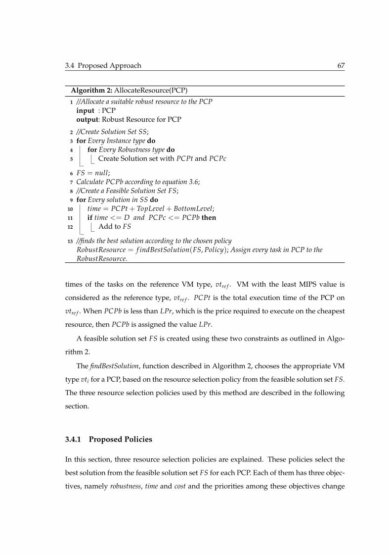
3.4 Proposed Approach 67
Algorithm 2: AllocateResource(PCP)
1 //Allocate a suitable robust resource to the PCPinput : PCPoutput: Robust Resource for PCP
2 //Create Solution Set SS;3 for Every Instance type do4 for Every Robustness type do5 Create Solution set with PCPt and PCPc
6 FS = null;7 Calculate PCPb according to equation 3.6;8 //Create a Feasible Solution Set FS;9 for Every solution in SS do
10 time = PCPt + TopLevel + BottomLevel;11 if time <= D and PCPc <= PCPb then12 Add to FS
13 //finds the best solution according to the chosen policyRobustResource = f indBestSolution(FS, Policy); Assign every task in PCP to theRobustResource.
times of the tasks on the reference VM type, vtre f . VM with the least MIPS value is
considered as the reference type, vtre f . PCPt is the total execution time of the PCP on
vtre f . When PCPb is less than LPr, which is the price required to execute on the cheapest
resource, then PCPb is assigned the value LPr.
A feasible solution set FS is created using these two constraints as outlined in Algo-
rithm 2.
The findBestSolution, function described in Algorithm 2, chooses the appropriate VM
type vti for a PCP, based on the resource selection policy from the feasible solution set FS.
The three resource selection policies used by this method are described in the following
section.
3.4.1 Proposed Policies
In this section, three resource selection policies are explained. These policies select the
best solution from the feasible solution set FS for each PCP. Each of them has three objec-
tives, namely robustness, time and cost and the priorities among these objectives change

68 Robust Scheduling with Deadline and Budget Constraints
for each of these policies. The description of the policies is given below:
1 Robustness-Cost-Time (RCT): The objective of this policy is to maximize robust-
ness and minimize cost and makespan. This policy sorts the feasible solution set
based on the robustness type, and among the solutions with the same robustness
type, they are sorted in the increasing order of cost. Solutions with the same ro-
bustness type and cost are sorted with increasing order of time. The best solution
from this sorted list is picked and the VM type with the associated robustness type
is mapped to the tasks of the PCP. Solutions chosen by this policy have high robust-
ness with a lower cost.
2 Robustness-Time-Cost (RTC): RTC policy is similar to RCT policy described above
with different priorities. This policy gives priority to robustness, followed by time
and finally cost. This policy selects a solution that is robust with lowest possible
makespan. Choices of RTC and RCT policies might have the same robustness type,
but will vary with respect to the VM type they select. RTC policy selects a solution
with high robustness and lowest possible makespan.
3 Weighted: With this policy users can define their own objective function using the
three parameters (robustness, time and cost) and assign weights for each of them.
Each value is normalized by taking the minimum and maximum values for that
parameter. The weights are applied to the normalized values of robustness, time
and cost, and based on these weights the best solution is selected. Weighted pol-
icy is a generalized policy, which can be used to find solutions according to user
preferences.
Our algorithm with the chosen policy finds a suitable VM type associated with a
robustness type for every PCP. Further, the algorithm allocates the PCP tasks on a VM of
the chosen type. The resource allocator, first attempts to find a VM of the specified type
among the running VMs. If such a VM is found, the algorithm checks if its end time is
less than the start time of the PCP. If this condition is satisfied, the algorithm allocates
PCP tasks on this existing VM; otherwise a new VM is created to allocate the tasks. This

3.5 Performance Evaluation 69
reduces the number of VMs instantiated and also minimizes the makespan as new VMs
take time to boot, which delays the schedule.
3.4.2 Fault-Tolerant Strategy
Checkpointing is employed in our algorithm as a fault-tolerant strategy. When a task
fails, the algorithm resumes the task from the last checkpoint and checkpointing of tasks
is done at regular intervals. The robustness type selected by the resource selection policy
provides the necessary slack for the failed task. Additionally, checkpointing strategy
helps to recover the task from the last checkpoint.
3.4.3 Time Complexity
Creating a Solution Set SS depends on the number of robustness types and VM types.
The time complexity for creating such a set is O(m.l), where m is the number of VM types
and l is the number of robustness types. The time complexity for sorting and choosing
the best solution based on the policy is O(m logm). The parameters m and l can take a
maximum value of n, where n is the number of tasks. Therefore, the time complexity
of AllocateResource is O(n2). The time complexity of FindPCP is O(n) as the maximum
number of times this method can be recursively invoked is equal to the number of tasks
n. Hence, the overall time complexity of our algorithm is O(n2).
3.5 Performance Evaluation
3.5.1 Simulation Setup
CloudSim [21] was used to simulate the cloud environment. It was extended to support
workflow applications, making it easy to define, deploy and schedule workflows. A
failure event generator was also integrated into the CloudSim, which generates failures
from an input failure trace. Five types of workflow applications and two failure models
are used in our simulation as described below.

70 Robust Scheduling with Deadline and Budget Constraints
Application Modeling
Three workflows (CyberShake, LIGO, and Montage) were considered. Their character-
istics are explained in detail by Bharathi et al. [74]. These workflows cover all the ba-
sic components such as, pipeline, data aggregration, data distribution and data redis-
tribution. Three different sizes of these workflows are chosen, small (around 30 tasks),
medium (around 100 tasks) and large (1000 tasks).
Resource Modeling
A cloud model with a single data center offering 10 different types of VMs is con-
sidered. The characteristics of VMs are modeled similar to the Amazon EC2 in-
stances (t1.micro, m1.small, m1.medium, m1.large, m1.xlarge, m2.xlarge, m2.2xlarge,
m2.4xlarge, c1.medium, c1.xlarge). A charging period of 60 minutes is considered for
these VMs, similar to the most prominent cloud providers.
Failure Modeling
Two types of failure models are considered for our experiments. First, failures are sim-
ulated from failure traces (FT). Due to lack of publicly available cloud specific failure
traces, Condor (CAE) Grid failure dataset [147], available as a part of Failure Trace
Archive [81] was chosen. Secondly, a failure model with 10% failure probability (FP)
is considered, i.e., for each node there is 10% probability of failure based on uniform dis-
tribution. The failed nodes may fail again with the same probability until they complete
their execution.
Each VM undergoes a performance variation, which affects the task execution time.
We model the variance in the task execution time as a normal distribution y = N(0, σ2),
where the standard deviation σ is 10% of the execution time of the task, as suggested
by Dejun et al. [44]. They have analyzed and presented the performance variations of
Amazon EC2 instances in their study.

3.5 Performance Evaluation 71
Reference Algorithms
Two reference algorithms to compare our resource allocation policies are implemented.
The first algorithm is a deadline constrained algorithm proposed by Abrishami et al. [5].
The IaaS cloud Partial Critical Path (ICPCP) algorithm, similar to our algorithm, divides
the workflow tasks into PCPs. ICPCP is non-robust algorithm bounded by a deadline
constraint.
The second reference algorithm implemented is a robust bi-objective genetic algo-
rithm (GA) [124]. This GA considers heterogeneous resources with the objective of max-
imizing the robustness by increasing the slack time between the tasks. This algorithm
considers deadline as a threshold and verifies that the schedule does not violate the dead-
line. The fitness function, selection and mutation operators for the GA are implemented
as described in [124]. The parameters of GA are set as follows: population size = 2000,
cross over probability = 0.9 and mutation probability = 0.1, as defined by the authors.
Maximum number of iterations is set to 800.
These algorithms are chosen for their similarity with our approach. ICPCP schedules
tasks by grouping them into PCPs, similar to our algorithm and GA tries to maximize the
slack time to be robust, which is the approach we adapt as well.
In this chapter, we have executed the experiments for three workflow applications
with two failure models. For each workflow, we varied the deadline with a fixed bud-
get and also varied the budget keeping the deadline fixed to measure the performance
with regards to robustness, makespan and cost. Each experiment was executed 10 times,
the mean of which is reported. For the weighted policy, the weights considered for ro-
bustness, time and cost are 0.5, 0.3 and 0.2 respectively. We intend to study the effect of
varying weights in future. We present our analysis and results in the following section.
3.5.2 Analysis and Results
The CyberShake workflow uses the Probabilistic Seismic Hazard Analysis (PSHA) tech-
nique to characterize earth-quake hazards in a region and the LIGO Workflow detects
gravitational waves of cosmic origin by observing stars and black holes [74]. We present

72 Robust Scheduling with Deadline and Budget Constraints
4.54.03.53.02.52.01.51.0
600
400
200
0
-200
-400
Deadline Factor
Mean of Tolerance Time
(a) Cybershake with fixed Budget and with FPfailure model
4.54.03.53.02.52.01.51.0
800
700
600
500
400
300
200
100
0
Budget Factor
Mean of Tolerance Time
(b) LIGO with fixed Deadline and with FT fail-ure model
4.54.03.53.02.52.01.51.0
600
400
200
0
-200
-400
Deadline
Mean of Safe Time
GA
ICPCP
RCT
RTC
Weighted
Line Plot of Mean( Safe Time )
Figure 3.1: Effect on robustness with tolerance time Rt
4.54.03.53.02.52.01.51.0
550
500
450
400
350
300
250
200
4.54.03.53.02.52.01.51.0
Actual
Deadline Factor
Mean of Makespan
Estimated
(a) Cybershake with fixed Budget and with FPfailure model
4.54.03.53.02.52.01.51.0
2400
2200
2000
1800
1600
1400
1200
1000
800
600
4.54.03.53.02.52.01.51.0
Actual
Budget Factor
Mean of MakeSpan
Estimated
(b) LIGO with fixed Deadline and with FT fail-ure model
4.54.03.53.02.52.01.51.0
600
400
200
0
-200
-400
Deadline
Mean of Safe Time
GA
ICPCP
RCT
RTC
Weighted
Line Plot of Mean( Safe Time )
Figure 3.2: Effect on makespan for large sized CyberShake and LIGO workflow
4.54.03.53.02.52.01.51.0
3000
2500
2000
1500
1000
500
4.54.03.53.02.52.01.51.0
Actual
Deadline Factor
Mean of Cost
Estimated
(a) Cybershake with fixed Budget and FP fail-ure model
4.54.03.53.02.52.01.51.0
16000
14000
12000
10000
8000
6000
4000
2000
4.54.03.53.02.52.01.51.0
Actual
Budget Factor
Mean of Cost
Estimated
(b) LIGO with fixed Deadline and with a FT fail-ure model
4.54.03.53.02.52.01.51.0
600
400
200
0
-200
-400
Deadline
Mean of Safe Time
GA
ICPCP
RCT
RTC
Weighted
Line Plot of Mean( Safe Time )
Figure 3.3: Effect on cost for large sized CyberShake and LIGO workflow
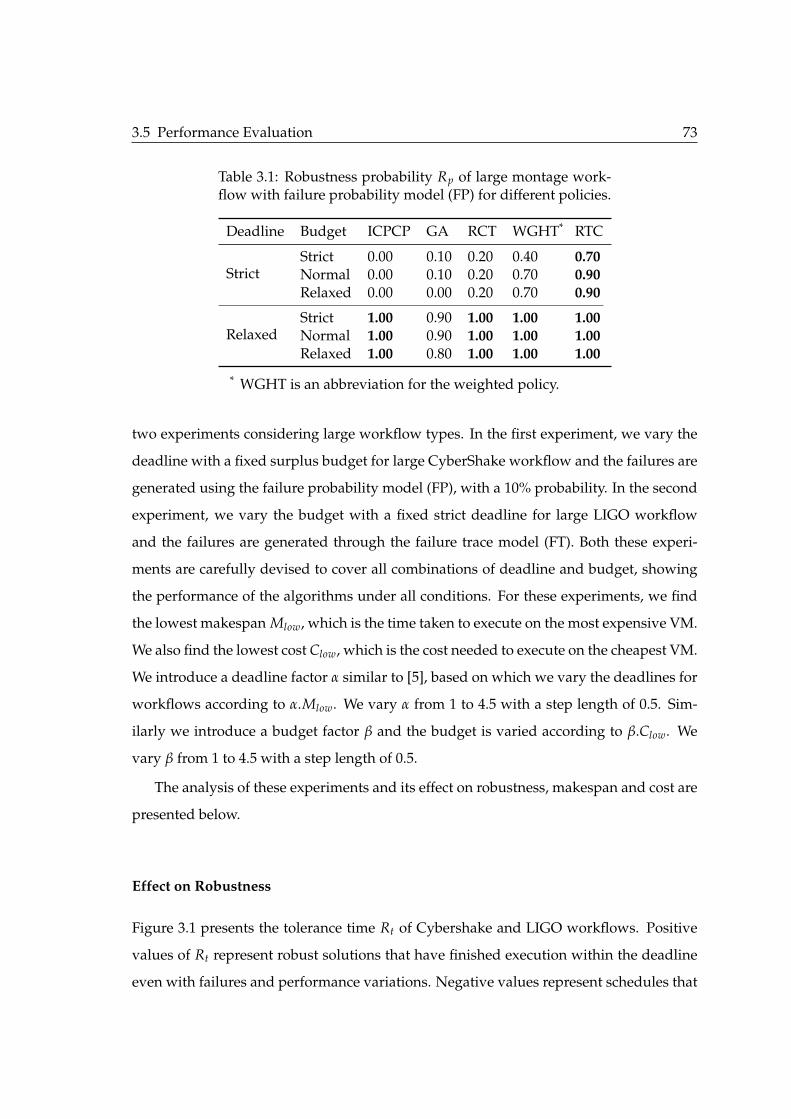
3.5 Performance Evaluation 73
Table 3.1: Robustness probability Rp of large montage work-flow with failure probability model (FP) for different policies.
Deadline Budget ICPCP GA RCT WGHT* RTC
StrictStrict 0.00 0.10 0.20 0.40 0.70Normal 0.00 0.10 0.20 0.70 0.90Relaxed 0.00 0.00 0.20 0.70 0.90
RelaxedStrict 1.00 0.90 1.00 1.00 1.00Normal 1.00 0.90 1.00 1.00 1.00Relaxed 1.00 0.80 1.00 1.00 1.00
* WGHT is an abbreviation for the weighted policy.
two experiments considering large workflow types. In the first experiment, we vary the
deadline with a fixed surplus budget for large CyberShake workflow and the failures are
generated using the failure probability model (FP), with a 10% probability. In the second
experiment, we vary the budget with a fixed strict deadline for large LIGO workflow
and the failures are generated through the failure trace model (FT). Both these experi-
ments are carefully devised to cover all combinations of deadline and budget, showing
the performance of the algorithms under all conditions. For these experiments, we find
the lowest makespan Mlow, which is the time taken to execute on the most expensive VM.
We also find the lowest cost Clow, which is the cost needed to execute on the cheapest VM.
We introduce a deadline factor α similar to [5], based on which we vary the deadlines for
workflows according to α.Mlow. We vary α from 1 to 4.5 with a step length of 0.5. Sim-
ilarly we introduce a budget factor β and the budget is varied according to β.Clow. We
vary β from 1 to 4.5 with a step length of 0.5.
The analysis of these experiments and its effect on robustness, makespan and cost are
presented below.
Effect on Robustness
Figure 3.1 presents the tolerance time Rt of Cybershake and LIGO workflows. Positive
values of Rt represent robust solutions that have finished execution within the deadline
even with failures and performance variations. Negative values represent schedules that
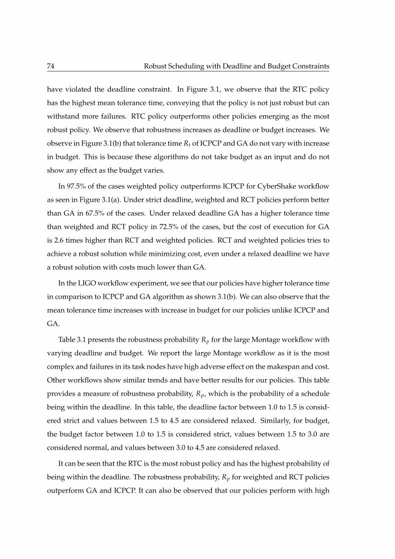
74 Robust Scheduling with Deadline and Budget Constraints
have violated the deadline constraint. In Figure 3.1, we observe that the RTC policy
has the highest mean tolerance time, conveying that the policy is not just robust but can
withstand more failures. RTC policy outperforms other policies emerging as the most
robust policy. We observe that robustness increases as deadline or budget increases. We
observe in Figure 3.1(b) that tolerance time Rt of ICPCP and GA do not vary with increase
in budget. This is because these algorithms do not take budget as an input and do not
show any effect as the budget varies.
In 97.5% of the cases weighted policy outperforms ICPCP for CyberShake workflow
as seen in Figure 3.1(a). Under strict deadline, weighted and RCT policies perform better
than GA in 67.5% of the cases. Under relaxed deadline GA has a higher tolerance time
than weighted and RCT policy in 72.5% of the cases, but the cost of execution for GA
is 2.6 times higher than RCT and weighted policies. RCT and weighted policies tries to
achieve a robust solution while minimizing cost, even under a relaxed deadline we have
a robust solution with costs much lower than GA.
In the LIGO workflow experiment, we see that our policies have higher tolerance time
in comparison to ICPCP and GA algorithm as shown 3.1(b). We can also observe that the
mean tolerance time increases with increase in budget for our policies unlike ICPCP and
GA.
Table 3.1 presents the robustness probability Rp for the large Montage workflow with
varying deadline and budget. We report the large Montage workflow as it is the most
complex and failures in its task nodes have high adverse effect on the makespan and cost.
Other workflows show similar trends and have better results for our policies. This table
provides a measure of robustness probability, Rp, which is the probability of a schedule
being within the deadline. In this table, the deadline factor between 1.0 to 1.5 is consid-
ered strict and values between 1.5 to 4.5 are considered relaxed. Similarly, for budget,
the budget factor between 1.0 to 1.5 is considered strict, values between 1.5 to 3.0 are
considered normal, and values between 3.0 to 4.5 are considered relaxed.
It can be seen that the RTC is the most robust policy and has the highest probability of
being within the deadline. The robustness probability, Rp for weighted and RCT policies
outperform GA and ICPCP. It can also be observed that our policies perform with high
3.5 Performance Evaluation 75
levels of robustness even under strict deadlines and budgets.
Effect on Makespan
Figure 3.2 shows the effect on makespan for CyberShake and LIGO workflows. Figures
3.2 and 3.3 have graphs with two panels, where the actual panel represents schedules
after execution with uncertainties and the estimated panel depicts schedules before exe-
cution without failures. Figures 3.2(a) and 3.2(b) show that makespan increases as dead-
line increases and makespan decreases as budget increases. Our policies have a higher
makespan when the schedule is estimated in comparison to ICPCP or GA; however the
actual makespan after failures and performance variations of resources is comparatively
minimal for our policies. RTC provides schedules with smallest makespan under the sce-
narios of failures and performance variations because it chooses robust resources with
least execution time. The average makespan of weighted policy is 19% lower than ICPCP
for both CyberShake and LIGO workflows. The average makespan of RCT policy is 14%
and 11% lower than ICPCP for CyberShake and LIGO workflows respectively.
In Figure 3.2(b), the estimated panel of the graph shows the working of the RTC pol-
icy. As the budget increases, the makespan increases steadily and then decreases steadily
as shown. This is because as the budget increases, the algorithm has the flexibility to
either add more slack time or choose an expensive VM. Therefore, with smaller increase
in budget, the algorithm chooses inexpensive VMs and adds slack time based on the in-
creases in budget, which increases the estimated makespan. With sufficient increase in
budget, the algorithm chooses expensive VM resulting in the decrease of the estimated
makespan. The actual panel of the graphs shows that the makespan of our policies are
much lower than ICPCP and GA. The RTC policy gives lower makespan consistently,
while the makespan of RCT and weighted policies increases slightly with increase in
deadline and decreases with increase in budget.
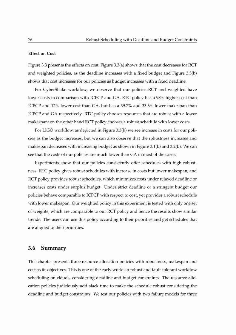
76 Robust Scheduling with Deadline and Budget Constraints
Effect on Cost
Figure 3.3 presents the effects on cost, Figure 3.3(a) shows that the cost decreases for RCT
and weighted policies, as the deadline increases with a fixed budget and Figure 3.3(b)
shows that cost increases for our policies as budget increases with a fixed deadline.
For CyberShake workflow, we observe that our policies RCT and weighted have
lower costs in comparison with ICPCP and GA. RTC policy has a 98% higher cost than
ICPCP and 12% lower cost than GA, but has a 39.7% and 33.6% lower makespan than
ICPCP and GA respectively. RTC policy chooses resources that are robust with a lower
makespan; on the other hand RCT policy chooses a robust schedule with lower costs.
For LIGO workflow, as depicted in Figure 3.3(b) we see increase in costs for our poli-
cies as the budget increases, but we can also observe that the robustness increases and
makespan decreases with increasing budget as shown in Figure 3.1(b) and 3.2(b). We can
see that the costs of our policies are much lower than GA in most of the cases.
Experiments show that our policies consistently offer schedules with high robust-
ness. RTC policy gives robust schedules with increase in costs but lower makespan, and
RCT policy provides robust schedules, which minimizes costs under relaxed deadline or
increases costs under surplus budget. Under strict deadline or a stringent budget our
policies behave comparable to ICPCP with respect to cost, yet provides a robust schedule
with lower makespan. Our weighted policy in this experiment is tested with only one set
of weights, which are comparable to our RCT policy and hence the results show similar
trends. The users can use this policy according to their priorities and get schedules that
are aligned to their priorities.
3.6 Summary
This chapter presents three resource allocation policies with robustness, makespan and
cost as its objectives. This is one of the early works in robust and fault-tolerant workflow
scheduling on clouds, considering deadline and budget constraints. The resource allo-
cation policies judiciously add slack time to make the schedule robust considering the
deadline and budget constraints. We test our policies with two failure models for three
3.6 Summary 77
scientific workflows with two metrics for robustness. Results indicated that our policies
are robust against uncertainties like task failures and performance variations of VMs. As
a future work, we propose to validate the proposed algorithm in a realistic cloud envi-
ronment.
Among the proposed policies presented, the RTC policy shows the highest robustness
and at the same time minimizes makespan of the workflow. The RCT policy provides a
robust schedule with costs marginally higher than the reference algorithms considered.
The weights of the weighted policy can be varied according to the user priorities. Overall,
our policies provide robust schedules with the lowest possible makespan. They also
show that with increase in budget, our policies increase the robustness of the schedule
with reasonable increase in cost.

This page intentionally left blank.
Chapter 4
Fault-Tolerant Scheduling Using SpotInstances
Scientific workflows are used to model applications of high throughput computation and complex
large scale data analysis. In recent years, Cloud computing is fast evolving as the target platform
for such applications among researchers. Furthermore, new pricing models have been pioneered
by Cloud providers that allow users to provision resources and to use them in an efficient manner
with significant cost reductions. In this chapter, we propose a scheduling algorithm that schedules
tasks on Cloud resources using two different pricing models (spot and on-demand instances) to
reduce the cost of execution whilst meeting the workflow deadline. The proposed algorithm is fault
tolerant against the premature termination of spot instances and also robust against performance
variations of Cloud resources. Experimental results demonstrate that our heuristic reduces up to
70% execution cost as against using only on-demand instances.
4.1 Introduction
CLOUD computing is increasingly used amidst researchers for scientific workflows
to perform high throughput computing and data analysis [89]. Numerous disci-
plines use scientific workflows to perform large scale complex analyses. Workflows en-
able scientists to easily define computational components, data and their dependencies
in a declarative way. This makes them easier to execute automatically, improving the ap-
plication performance, and reducing the time required to obtain scientific results [75,76].
Clouds are realizing the vision of utility computing by delivering computing re-
sources as services. This is facilitating Cloud providers to evolve various business models
79
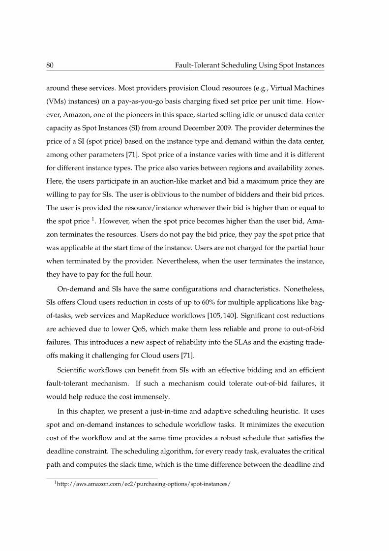
80 Fault-Tolerant Scheduling Using Spot Instances
around these services. Most providers provision Cloud resources (e.g., Virtual Machines
(VMs) instances) on a pay-as-you-go basis charging fixed set price per unit time. How-
ever, Amazon, one of the pioneers in this space, started selling idle or unused data center
capacity as Spot Instances (SI) from around December 2009. The provider determines the
price of a SI (spot price) based on the instance type and demand within the data center,
among other parameters [71]. Spot price of a instance varies with time and it is different
for different instance types. The price also varies between regions and availability zones.
Here, the users participate in an auction-like market and bid a maximum price they are
willing to pay for SIs. The user is oblivious to the number of bidders and their bid prices.
The user is provided the resource/instance whenever their bid is higher than or equal to
the spot price 1. However, when the spot price becomes higher than the user bid, Ama-
zon terminates the resources. Users do not pay the bid price, they pay the spot price that
was applicable at the start time of the instance. Users are not charged for the partial hour
when terminated by the provider. Nevertheless, when the user terminates the instance,
they have to pay for the full hour.
On-demand and SIs have the same configurations and characteristics. Nonetheless,
SIs offers Cloud users reduction in costs of up to 60% for multiple applications like bag-
of-tasks, web services and MapReduce workflows [105, 140]. Significant cost reductions
are achieved due to lower QoS, which make them less reliable and prone to out-of-bid
failures. This introduces a new aspect of reliability into the SLAs and the existing trade-
offs making it challenging for Cloud users [71].
Scientific workflows can benefit from SIs with an effective bidding and an efficient
fault-tolerant mechanism. If such a mechanism could tolerate out-of-bid failures, it
would help reduce the cost immensely.
In this chapter, we present a just-in-time and adaptive scheduling heuristic. It uses
spot and on-demand instances to schedule workflow tasks. It minimizes the execution
cost of the workflow and at the same time provides a robust schedule that satisfies the
deadline constraint. The scheduling algorithm, for every ready task, evaluates the critical
path and computes the slack time, which is the time difference between the deadline and
1http://aws.amazon.com/ec2/purchasing-options/spot-instances/
4.2 Related Work 81
the critical path time. The main motivation of the work is to exploit SIs to the extent
possible within the slack time. As the slack time decreases due to failures or performance
variations in the system, the algorithm adaptively switches to on-demand instances. The
algorithm employs a bidding strategy and checkpointing to minimize cost and to comply
with the deadline constraint. Checkpointing can tolerate instance failures and reduce
execution cost, in spite of an inherent overhead [120] .
The key contributions of this chapter are: 1) A just in-time scheduling heuristic that
uses spot and on-demand resources to schedule workflow tasks in a robust manner. 2)
An intelligent bidding strategy that minimizes cost.
4.2 Related Work
Multiple applications use SIs for resource provisioning. Voorsluys et al. [140] use SIs to
provision compute-intensive bag-of-tasks jobs constrained by deadline. They show that
applications can run faster and economically by reducing costs up to 60%. However, they
use a bag-of-task application and use only SIs to execute the jobs. Mazzucco et al. [96]
exploit SIs for providing web services as a Software-as-a-Service(SaaS). They develop an
optimal and truthful bidding scheme to optimize revenue. Chohan et al. [29] similarly
use SIs for MapReduce workflows to reduce costs and also detail the effects of prema-
ture failures. Ostermann et al. [105] study the impact of using SI with grid resources for
scientific workflows. They use SIs when grid resources are not available and use static
bidding mechanism to show reduction in cost.
In this work, we schedule workflow tasks entirely on Cloud resources, exploiting both
spot and on-demand instances to minimize the cost. This work presents a dynamic and
adaptive scheduling heuristic, whilst providing a robust schedule. An intelligent and
adaptive bidding strategy is also presented, which bids such that the price is minimized.
Amazon does not reveal the details of spot price modeling and their market strategies.
Therefore, understanding the dynamics of the market and the frequency of price changes
is crucial for bidding effectively. Javadi et al. [71] provide a comprehensive analysis of
SIs. They analyze the spot market with respect to two parameters: spot price and inter-

82 Fault-Tolerant Scheduling Using Spot Instances
price time i.e. the time between price changes. They also propose a statistical model
representing the spot price dynamics as a mixture of Gaussian distributions and inter-
price time as an exponential distribution, which models spot price with a high degree of
accuracy.
Yehuda et al. [11] provide a model through reverse engineering. They speculate that
prices are not always market-driven, but generated randomly via a dynamic hidden re-
serve price. Reserve price is a hidden price below which Amazon ignores all bids. These
works give a deeper understanding of the price dynamics of the spot market and help in
modeling the same.
Yi et al. [3] have simulated how checkpointing policies reduce costs of computations
by providing fault-tolerance using EC2 SIs. Their evaluation shows that in spite of the
inherent overhead, checkpointing schemes can tolerate instance failures. We also use
checkpointing policy as a fault-tolerant mechanism and to further reduce computation
costs.
The details of our system model and heuristics are discussed in the following sections.
4.3 Background
A Workflow is represented as a Directed Acyclic Graph (DAG), as mentioned in Section
3.3. Each workflow is bounded by a user defined deadline D. We also account for data
transfer time between tasks. The data transfer time between two tasks is calculated based
on the size of the data transferred and the Cloud data center internal network bandwidth.
Additionally, each workflow task tj also has a task length lenj given in Million Instruc-
tions, which is used to estimate the task execution time. For each workflow, a dummy
exit and entry node is added to have one start and end node.
Makespan, M, is the total elapsed time required to execute the entire workflow. The
deadline D is considered as a constraint, where makespan should not be more than the
deadline (M 6 D). The makespan of the workflow is computed as M = f inishtn −
ST, where ST is the submission time and f inishtn is finish time of the exit node of the
workflow.
4.3 Background 83
Pricing models: In our model, we adapt two types of instances from the Amazon
model, which vary in their pricing structure. The two pricing models considered are:
1) On-Demand instance: the user pays by the hour based on the instance type. 2) Spot
Instance: users bid for the instance and it is made available as long as their bid is higher
than the spot price. Spot prices change dynamically and it can change during the instance
runtime. The price of a SI (spot price) is determined by the provider based on the instance
type and demand within the data center, among other parameters [71].
Critical Path, CP, is the longest path from the start node to the exit node of the work-
flow. Critical path determines the makespan of a workflow. The critical path is evaluated
in a breadth-first manner calculating the weights of each node. The node weight is the
maximum among the predecessors’ estimated finish time and the data transfer time cal-
culated as per Equation 4.1 given by Topcuoglu et al. [135],
weight(ti) = maxtp∈pred(ti)
{weight(tp) + wp + cp,i} (4.1)
where, pred(ti) is all the parent nodes of ti, wi is the execution time of node ti on an
instance type chosen by the algorithm. cp,i is the data transfer time from node ti to tp. The
maximum weight among the exit nodes is the critical path time. When a node completes
execution its weight and data transfer time to all its child nodes is made zero, and the
critical path is recomputed.
Latest Time to On-Demand, LTO is the latest time the algorithm has to switch to
on-demand instances to satisfy the deadline constraint. The algorithm exploits the spot
market before the LTO and switches to on-demand instance later. LTO aids in choosing
the right instance, to speed up or slow down and choose the apt pricing model. It is
determined for every ready task and the scheduling decisions are made based on the
current time t and the LTO. LTO at time t is the difference between the deadline and the
critical path (LTOt = D− CPt).
Total Cost, C, is the sum of the cost of all the instances used for the workflow ex-
ecution, based on their instance type and pricing model. The cost of each instance is
calculated as per the Amazon model. If the instance is an on-demand instance, the on-
demand price of that instance is used. If the instance is spot, the spot price of the instance

84 Fault-Tolerant Scheduling Using Spot Instances
Figure 4.1: System architecture.
is used to calculate the cost. All partial hours are rounded up to full hours for both spot
and on-demand instances (e.g. 5.1 hours is rounded up to 6 hours).
4.4 System Model
The system architecture is presented in Figure 4.1. The workflow engine acts as a middle
layer between the user application and the Cloud. Users submit a workflow application
into the engine, which schedules the workflow tasks, provides fault tolerance mecha-
nism, and allocates resources in a transparent manner.
The Dispatcher analyses the data and/or control dependencies between the tasks and
submits the ready tasks to the task scheduler. Ready tasks are those tasks whose prede-
cessor tasks have completed their execution and have received all input files, and are
prepared to be scheduled.
Fault Tolerant Strategy : SIs are prone to out-of-bid failures and an efficient fault toler-
ant strategy is crucial for a deadline constraint workflow scheduling. Checkpointing is an
effective fault tolerant mechanism [120] for spot markets, it takes a snapshot periodically
and saves redundant computation in case of failure. It is especially useful in a SI scenario
as we save partial computation in the event of failure and do not pay for that. We use

4.4 System Model 85
checkpointing mechanism as a fault tolerant strategy. Checkpoints are taken periodically
at a user defined frequency. A static checkpointing overhead time is taken into account.
However, the cost of storing checkpoints is not considered, as the price of storage service
is negligible compared to cost of VMs [120]. Moreover, checkpointing can be done in par-
allel with the computation, so the time taken to transfer checkpointing data is ignored as
it is insignificant.
Resource Allocation: Task scheduler chooses Cloud resource type and also the pric-
ing model (e.g. spot or on-demand). This module allocates the appropriate resource as
chosen by the task scheduler.
The task scheduler employs a scheduling algorithm to find a suitable Cloud resource
for every task. The details of the scheduling algorithm are outlined in the next section.
Runtime Estimation: To determine the runtime of a workflow task on a particular
instance type, we use Downey’s analytical model [47]. Downey’s model requires a task’s
average parallelism A, coefficient of variance of parallelism σ, the task length and the
number of cores of the target instance type to estimate the runtime. We have used the
model of Cirne et al. [30] for generating the values of A and σ for each task. This model
has been shown to capture the behavior of moldable jobs in parallel production envi-
ronments. With the use of these two models the task’s runtime is estimated on different
instance types.
Failure Estimator estimates the failure probability, FP of a particular bid price (bidt)
based on the spot price history. The history price of one month prior to the start of the
execution and the spot prices until the point of estimation is used. The failure probability
estimator analyzes the spot price history for the bid value in consideration, for which
the total time of the spot price history, HT, and the total out of bid time, OBTbidt for the
bid bidt is measured. The total out of bid time is the aggregated time in history when
the spot price was higher than the bid bidt. These two factors are used to estimate the
probability of failure as shown in Equation 4.2. This estimation is used while evaluating
the bid value and also while scheduling the task.
FPbidt = OBTbidt /HT (4.2)
86 Fault-Tolerant Scheduling Using Spot Instances
The problem we address in this work is to find a mapping of workflow tasks onto
heterogeneous VM types, using a mixture of on-demand and SIs such that the cost of
workflow execution is minimized within the deadline. The schedule should also be ro-
bust against premature termination of SIs and performance variations of the resources.
Assumptions: Data transfer cost between VMs are considered to be zero, as in most
public Clouds, data transfer inside a Cloud data center is free. The data center is assumed
to have sufficient resources, avoiding VM rejections due to resource contention. This is
not a prohibitive assumption as the resources required are much smaller than the data
center capacity. The number of VM types available and the number of VM types used by
the workflow engine are known and limited. Additionally, only one task is executed on
an instance at a particular time
4.5 Proposed Approach
4.5.1 Scheduling Algorithm
The proposed just in-time scheduling algorithm maps ready tasks submitted by the task
dispatcher onto Cloud resources. It selects a suitable instance type based on the deadline
constraint and the LTO. The algorithm along with a suitable instance type also selects an
apt pricing model to minimize the overall cost. The outline of the algorithm is given in
Algorithm 3. Mapping workflow tasks onto heterogeneous instance types with different
pricing models is a well known NP-complete problem [73]. Hence, we propose a heuristic
to address the same.
The crux of the algorithm is to map tasks that arrive before the LTO to SIs and those
that arrive after the LTO to on-demand instances. In this approach, a single SI type is
used. This instance has lowest cost. The rationale behind this is to minimize the overall
execution cost. On the other hand, multiple types of on-demand instances are used. This
helps to speed up and slow down execution.
Initially, CP and LTO are computed before the workflow execution. They are recom-
puted for all ready tasks during execution. Whilst recomputing the CP time, if there are
any running tasks in the critical path, the time left for their execution is only accounted.
4.5 Proposed Approach 87
This reflects a realistic CP time at that point, giving the algorithm a strong approximation
of the time left for the completion of the workflow.
Run time of a particular task varies with different instance types. Similarly, the critical
path also varies depending on the instance type used to estimate the same. Henceforth,
the LTO also varies accordingly. The scheduling decision changes depending on the in-
stance type used to estimate the critical path. We have developed two algorithms keeping
this aspect in consideration, namely Conservative and Aggressive.
Conservative algorithm: it estimates the CP and LTO on the lowest cost instance
type. The CP estimated in this approach is usually the longest. Hence, it uses SIs only
when the deadlines are relaxed. Under tight and moderate deadlines, it does not generate
enough slack time to utilize SIs and therefore maps tasks predominantly to on-demand
instances. It is conservative in approach and utilizes SIs in a cautious manner only under
relaxed deadline making it more robust.
Aggressive algorithm: it estimates the CP and LTO on a highest cost instance type.
Here, the CP is smaller than the Conservative algorithm. This approach generates more
slack time than the Conservative algorithm and therefore uses SIs even with a strict dead-
line. This offers significant reduction in cost under moderately relaxed deadline. Under
relaxed deadline both algorithms perform similarly. When the market is volatile inducing
failures, this approach has less slack time. Hence, it has to opt for on-demand instances
that are expensive, increasing the overall cost. The performance of these two algorithms
is investigated in the evaluation section.
Algorithm 5 outlines the generic heuristic, which is common to both Conservative
and the Aggressive algorithms. When a new task is ready to be mapped, the algorithm
through the method FindFreeSpace tries to pick free slots among the existing running in-
stances. Free slots are those time slots in an active running instance, when no task is
being executed. If there is no free slot it searches for a running instance that will be free
before the task’s latest start time. Latest start time is the latest time a task can start its ex-
ecution such that the whole workflow can finish within the deadline. Finding such free
slots reduces cost as the algorithm avoids creating new instances for every task. This also
saves time as the initiation time for starting a new instance is avoided. Additionally, the
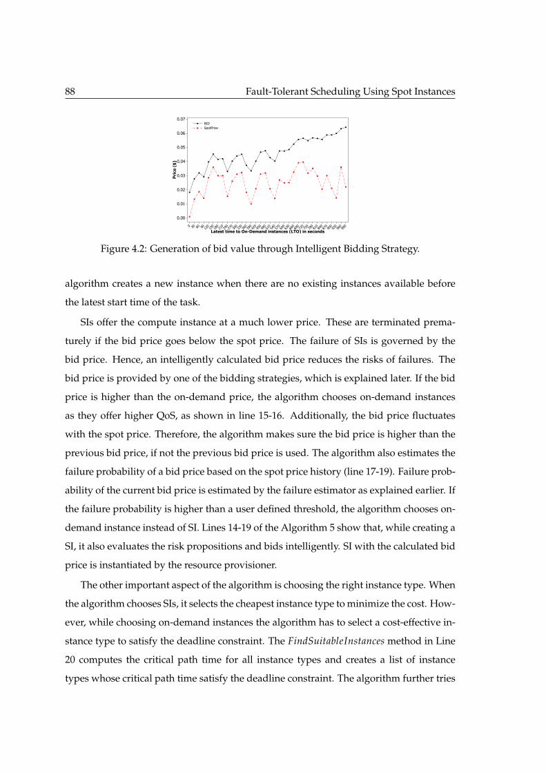
88 Fault-Tolerant Scheduling Using Spot Instances
990
960
930
900
870
840
810
780
750
720
690
660
630
600
570
540
510
480
450
420
390
360
330
300
270
240
210
180
150
1209060300
0.07
0.06
0.05
0.04
0.03
0.02
0.01
0.00
Latest time to On-Demand instances (LTO) in seconds
Price ($)
BID
SpotPrice
Figure 4.2: Generation of bid value through Intelligent Bidding Strategy.
algorithm creates a new instance when there are no existing instances available before
the latest start time of the task.
SIs offer the compute instance at a much lower price. These are terminated prema-
turely if the bid price goes below the spot price. The failure of SIs is governed by the
bid price. Hence, an intelligently calculated bid price reduces the risks of failures. The
bid price is provided by one of the bidding strategies, which is explained later. If the bid
price is higher than the on-demand price, the algorithm chooses on-demand instances
as they offer higher QoS, as shown in line 15-16. Additionally, the bid price fluctuates
with the spot price. Therefore, the algorithm makes sure the bid price is higher than the
previous bid price, if not the previous bid price is used. The algorithm also estimates the
failure probability of a bid price based on the spot price history (line 17-19). Failure prob-
ability of the current bid price is estimated by the failure estimator as explained earlier. If
the failure probability is higher than a user defined threshold, the algorithm chooses on-
demand instance instead of SI. Lines 14-19 of the Algorithm 5 show that, while creating a
SI, it also evaluates the risk propositions and bids intelligently. SI with the calculated bid
price is instantiated by the resource provisioner.
The other important aspect of the algorithm is choosing the right instance type. When
the algorithm chooses SIs, it selects the cheapest instance type to minimize the cost. How-
ever, while choosing on-demand instances the algorithm has to select a cost-effective in-
stance type to satisfy the deadline constraint. The FindSuitableInstances method in Line
20 computes the critical path time for all instance types and creates a list of instance
types whose critical path time satisfy the deadline constraint. The algorithm further tries
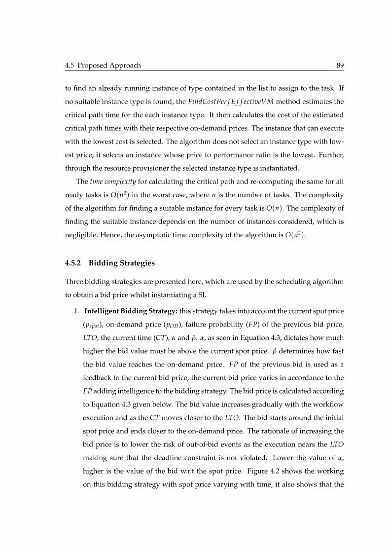
4.5 Proposed Approach 89
to find an already running instance of type contained in the list to assign to the task. If
no suitable instance type is found, the FindCostPer f E f f ectiveVM method estimates the
critical path time for the each instance type. It then calculates the cost of the estimated
critical path times with their respective on-demand prices. The instance that can execute
with the lowest cost is selected. The algorithm does not select an instance type with low-
est price, it selects an instance whose price to performance ratio is the lowest. Further,
through the resource provisioner the selected instance type is instantiated.
The time complexity for calculating the critical path and re-computing the same for all
ready tasks is O(n2) in the worst case, where n is the number of tasks. The complexity
of the algorithm for finding a suitable instance for every task is O(n). The complexity of
finding the suitable instance depends on the number of instances considered, which is
negligible. Hence, the asymptotic time complexity of the algorithm is O(n2).
4.5.2 Bidding Strategies
Three bidding strategies are presented here, which are used by the scheduling algorithm
to obtain a bid price whilst instantiating a SI.
1. Intelligent Bidding Strategy: this strategy takes into account the current spot price
(pspot), on-demand price (pOD), failure probability (FP) of the previous bid price,
LTO, the current time (CT), α and β. α, as seen in Equation 4.3, dictates how much
higher the bid value must be above the current spot price. β determines how fast
the bid value reaches the on-demand price. FP of the previous bid is used as a
feedback to the current bid price, the current bid price varies in accordance to the
FP adding intelligence to the bidding strategy. The bid price is calculated according
to Equation 4.3 given below. The bid value increases gradually with the workflow
execution and as the CT moves closer to the LTO. The bid starts around the initial
spot price and ends closer to the on-demand price. The rationale of increasing the
bid price is to lower the risk of out-of-bid events as the execution nears the LTO
making sure that the deadline constraint is not violated. Lower the value of α,
higher is the value of the bid w.r.t the spot price. Figure 4.2 shows the working
on this bidding strategy with spot price varying with time, it also shows that the

90 Fault-Tolerant Scheduling Using Spot Instances
Algorithm 3: Schedule(t)input : task ti
1 vms← all VMs currently in the pool;2 types← available instance types;3 estimates← compute estimated runtime of task ti on each type ∈ types;4 Recompute CP and LTO.5 timeLe f t = LTO− currentTime6 if timeLeft > 0 then7 decision← FindFreeSpace(ti, vms, PriceModel.ANY);8 if decision.allocated = true return decision;9 if decision.allocated = false then
10 decision← FindRunningVM(ti, vms, PriceModel.ANY);11 if decision.allocated = true return decision;
12 timeLe f t = timeLe f t− vmInitTime13 if timeLeft > 0 then14 bid← EstimateBidPrice(ti, type);15 if bid > on-demand price then16 Map to on-demand instance and return decision.
17 failProb← EstimateFailureProbability(bid);18 if failProb < threshold then19 Map to spot instance and return decision;
20 InstanceList← FindSuitableInstances(CP, D)21 decision← FindFreeSpace(ti, InstanceList, PriceModel.ONDEMAND);22 if decision.allocated = true return decision;23 if decision.allocated = false then24 decision← FindRunningVM(ti, InstanceList, PriceModel.ONDEMAND);25 if decision.allocated = true return decision;
26 // If no running instance is found from InstanceList return decision←FindCostPerfEffectiveVM(ti, InstanceList);
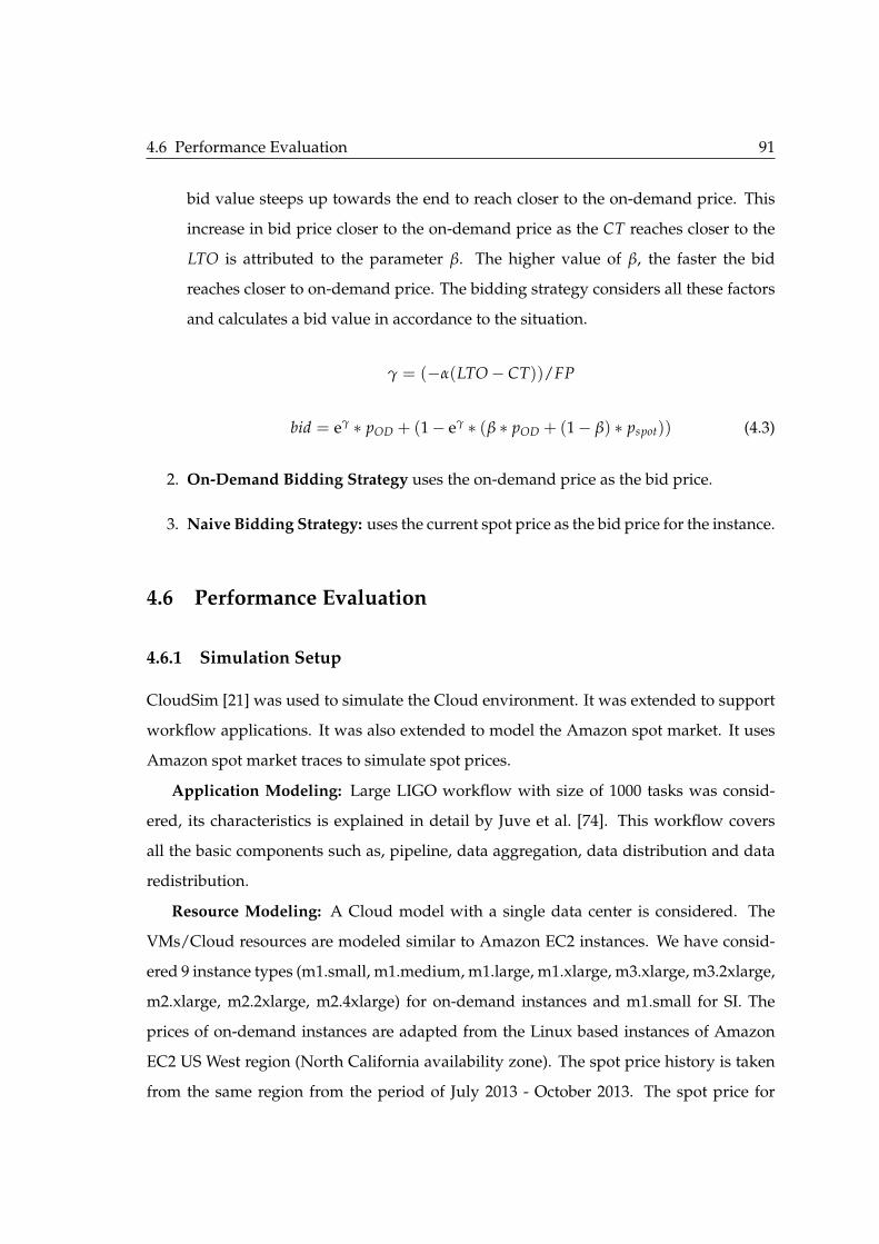
4.6 Performance Evaluation 91
bid value steeps up towards the end to reach closer to the on-demand price. This
increase in bid price closer to the on-demand price as the CT reaches closer to the
LTO is attributed to the parameter β. The higher value of β, the faster the bid
reaches closer to on-demand price. The bidding strategy considers all these factors
and calculates a bid value in accordance to the situation.
γ = (−α(LTO− CT))/FP
bid = eγ ∗ pOD + (1− eγ ∗ (β ∗ pOD + (1− β) ∗ pspot)) (4.3)
2. On-Demand Bidding Strategy uses the on-demand price as the bid price.
3. Naive Bidding Strategy: uses the current spot price as the bid price for the instance.
4.6 Performance Evaluation
4.6.1 Simulation Setup
CloudSim [21] was used to simulate the Cloud environment. It was extended to support
workflow applications. It was also extended to model the Amazon spot market. It uses
Amazon spot market traces to simulate spot prices.
Application Modeling: Large LIGO workflow with size of 1000 tasks was consid-
ered, its characteristics is explained in detail by Juve et al. [74]. This workflow covers
all the basic components such as, pipeline, data aggregation, data distribution and data
redistribution.
Resource Modeling: A Cloud model with a single data center is considered. The
VMs/Cloud resources are modeled similar to Amazon EC2 instances. We have consid-
ered 9 instance types (m1.small, m1.medium, m1.large, m1.xlarge, m3.xlarge, m3.2xlarge,
m2.xlarge, m2.2xlarge, m2.4xlarge) for on-demand instances and m1.small for SI. The
prices of on-demand instances are adapted from the Linux based instances of Amazon
EC2 US West region (North California availability zone). The spot price history is taken
from the same region from the period of July 2013 - October 2013. The spot price for
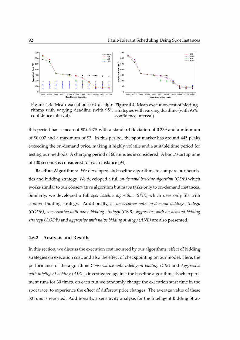
92 Fault-Tolerant Scheduling Using Spot Instances
1500001400001300001200001100001000009000080000700006000050000
700
600
500
400
300
200
100
0
Execution Cost ($)
ODB
CIB
AIB
SPB
Deadline in seconds
Figure 4.3: Mean execution cost of algo-rithms with varying deadline (with 95%confidence interval).
1500001400001300001200001100001000009000080000700006000050000
700
600
500
400
300
200
100
0
Execution Cost ($)
CIB
CODB
AIB
AODB
Deadline in Seconds
Figure 4.4: Mean execution cost of biddingstrategies with varying deadline (with 95%confidence interval).
this period has a mean of $0.05475 with a standard deviation of 0.239 and a minimum
of $0.007 and a maximum of $3. In this period, the spot market has around 445 peaks
exceeding the on-demand price, making it highly volatile and a suitable time period for
testing our methods. A charging period of 60 minutes is considered. A boot/startup time
of 100 seconds is considered for each instance [94].
Baseline Algorithms: We developed six baseline algorithms to compare our heuris-
tics and bidding strategy. We developed a full on-demand baseline algorithm (ODB) which
works similar to our conservative algorithm but maps tasks only to on-demand instances.
Similarly, we developed a full spot baseline algorithm (SPB), which uses only SIs with
a naive bidding strategy. Additionally, a conservative with on-demand bidding strategy
(CODB), conservative with naive bidding strategy (CNB), aggressive with on-demand bidding
strategy (AODB) and aggressive with naive bidding strategy (ANB) are also presented.
4.6.2 Analysis and Results
In this section, we discuss the execution cost incurred by our algorithms, effect of bidding
strategies on execution cost, and also the effect of checkpointing on our model. Here, the
performance of the algorithms Conservative with intelligent bidding (CIB) and Aggressive
with intelligent bidding (AIB) is investigated against the baseline algorithms. Each experi-
ment runs for 30 times, on each run we randomly change the execution start time in the
spot trace, to experience the effect of different price changes. The average value of these
30 runs is reported. Additionally, a sensitivity analysis for the Intelligent Bidding Strat-
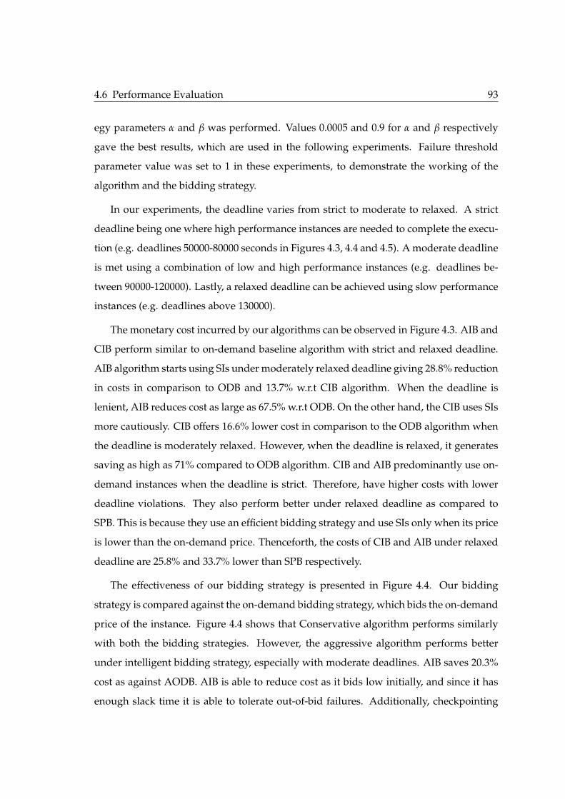
4.6 Performance Evaluation 93
egy parameters α and β was performed. Values 0.0005 and 0.9 for α and β respectively
gave the best results, which are used in the following experiments. Failure threshold
parameter value was set to 1 in these experiments, to demonstrate the working of the
algorithm and the bidding strategy.
In our experiments, the deadline varies from strict to moderate to relaxed. A strict
deadline being one where high performance instances are needed to complete the execu-
tion (e.g. deadlines 50000-80000 seconds in Figures 4.3, 4.4 and 4.5). A moderate deadline
is met using a combination of low and high performance instances (e.g. deadlines be-
tween 90000-120000). Lastly, a relaxed deadline can be achieved using slow performance
instances (e.g. deadlines above 130000).
The monetary cost incurred by our algorithms can be observed in Figure 4.3. AIB and
CIB perform similar to on-demand baseline algorithm with strict and relaxed deadline.
AIB algorithm starts using SIs under moderately relaxed deadline giving 28.8% reduction
in costs in comparison to ODB and 13.7% w.r.t CIB algorithm. When the deadline is
lenient, AIB reduces cost as large as 67.5% w.r.t ODB. On the other hand, the CIB uses SIs
more cautiously. CIB offers 16.6% lower cost in comparison to the ODB algorithm when
the deadline is moderately relaxed. However, when the deadline is relaxed, it generates
saving as high as 71% compared to ODB algorithm. CIB and AIB predominantly use on-
demand instances when the deadline is strict. Therefore, have higher costs with lower
deadline violations. They also perform better under relaxed deadline as compared to
SPB. This is because they use an efficient bidding strategy and use SIs only when its price
is lower than the on-demand price. Thenceforth, the costs of CIB and AIB under relaxed
deadline are 25.8% and 33.7% lower than SPB respectively.
The effectiveness of our bidding strategy is presented in Figure 4.4. Our bidding
strategy is compared against the on-demand bidding strategy, which bids the on-demand
price of the instance. Figure 4.4 shows that Conservative algorithm performs similarly
with both the bidding strategies. However, the aggressive algorithm performs better
under intelligent bidding strategy, especially with moderate deadlines. AIB saves 20.3%
cost as against AODB. AIB is able to reduce cost as it bids low initially, and since it has
enough slack time it is able to tolerate out-of-bid failures. Additionally, checkpointing
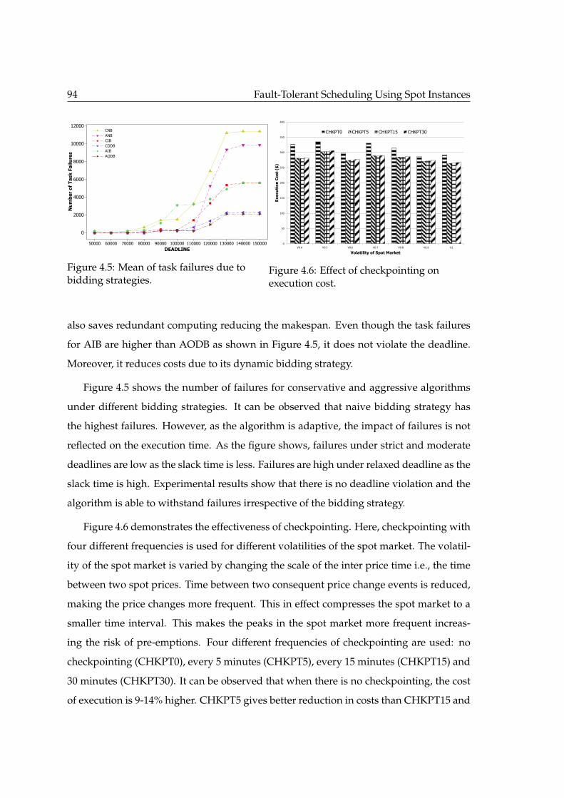
94 Fault-Tolerant Scheduling Using Spot Instances
1500001400001300001200001100001000009000080000700006000050000
12000
10000
8000
6000
4000
2000
0
DEADLINE
Number of Task Failures
CNB
ANB
CIB
CODB
AIB
AODB
Figure 4.5: Mean of task failures due tobidding strategies.
0
50
100
150
200
250
300
350
400
V0.4 V0.5 V0.6 V0.7 V0.8 V0.9 V1
Ex
ecu
tio
n C
ost
($)
Volatility of Spot Market
CHKPT0 CHKPT5 CHKPT15 CHKPT30
Figure 4.6: Effect of checkpointing onexecution cost.
also saves redundant computing reducing the makespan. Even though the task failures
for AIB are higher than AODB as shown in Figure 4.5, it does not violate the deadline.
Moreover, it reduces costs due to its dynamic bidding strategy.
Figure 4.5 shows the number of failures for conservative and aggressive algorithms
under different bidding strategies. It can be observed that naive bidding strategy has
the highest failures. However, as the algorithm is adaptive, the impact of failures is not
reflected on the execution time. As the figure shows, failures under strict and moderate
deadlines are low as the slack time is less. Failures are high under relaxed deadline as the
slack time is high. Experimental results show that there is no deadline violation and the
algorithm is able to withstand failures irrespective of the bidding strategy.
Figure 4.6 demonstrates the effectiveness of checkpointing. Here, checkpointing with
four different frequencies is used for different volatilities of the spot market. The volatil-
ity of the spot market is varied by changing the scale of the inter price time i.e., the time
between two spot prices. Time between two consequent price change events is reduced,
making the price changes more frequent. This in effect compresses the spot market to a
smaller time interval. This makes the peaks in the spot market more frequent increas-
ing the risk of pre-emptions. Four different frequencies of checkpointing are used: no
checkpointing (CHKPT0), every 5 minutes (CHKPT5), every 15 minutes (CHKPT15) and
30 minutes (CHKPT30). It can be observed that when there is no checkpointing, the cost
of execution is 9-14% higher. CHKPT5 gives better reduction in costs than CHKPT15 and

4.7 Summary 95
CHKPT30. It can be observed that the execution cost between the CHKPT5, CHKPT15
and CHKPT30 are comparable without significant difference. This can be attributed to
low spot prices, the price history we have considered has 82.7% of price changes below
$0.01. Therefore, when the average spot price is higher, we will observe a significant dif-
ference. Under the spot market considered, CHKPT30 is better as the overhead is lower
than CHKPT5, CHKPT15.
4.7 Summary
In this chapter, two scheduling heuristics that map workflow tasks onto spot and on-
demand instance are presented. They minimize the execution cost. They are shown to
be robust and fault-tolerant towards out-of-bid failures and performance variations of
Cloud instances. A bidding strategy that bids in accordance to the workflow require-
ments to minimize the cost is also presented. This work also demonstrates the use of
checkpointing and offers cost savings up to 14%. Simulation results show that cost re-
ductions of upto 70% are achieved under relaxed deadlines, when SIs are used.

This page intentionally left blank.

Chapter 5
Reliable Workflow Execution UsingReplication and Spot Instances
Cloud environments offer low-cost computing resources as a subscription-based service. These
resources are elastically scalable and dynamically provisioned. Furthermore, cloud providers have
also pioneered new pricing models like spot instances that are cost-effective. As a result, scientific
workflows are increasingly adopting cloud computing. However, spot instances are terminated
when the market price exceeds the users bid price. Likewise, cloud is not a utopian environment.
Failures are inevitable in such large complex distributed systems. It is also well studied that
cloud resources experience fluctuations in the delivered performance. These challenges make fault-
tolerance an important criterion in workflow scheduling. This chapter presents an adaptive, just-
in time scheduling algorithm for scientific workflows. This algorithm judiciously uses both spot
and on-demand instances to reduce cost and provide fault-tolerance. The proposed scheduling
algorithm also consolidates resources to further minimize execution time and cost. Extensive
simulations show that the proposed heuristics are fault-tolerant and effective, especially under
short deadlines, providing robust schedules with the lowest possible makespan and cost.
5.1 Introduction
ALTHOUGH, scheduling scientific workflows on cloud will immensely reduce cost
and makespan. Cloud computing, like any other distributed system, is also prone
to resource failures. These failures are generally due to software faults, hardware faults,
errors in network, data staging issues, failures due to virtualization, disk errors, power
issues and many others. These failures from a workflow application perspective can
97
98 Reliable Workflow Execution Using Replication and Spot Instances
be classified into 1) task failures, 2) VM failures, and 3) workflow level failures [67].
Nonetheless, failures are inevitable whilst running a complex application like workflows
consisting of thousands of tasks.
Furthermore, cloud resources also experience performance variations because of re-
source sharing, consolidation and migration among other factors. Performance variation
of cloud resources affects the overall execution time (i.e. makespan) of the workflow.
It further increases the difficulty to estimate the task execution time accurately. Dejun
et al. [44] show that the behavior of multiple “identical” resources vary in performance
while serving exactly the same workload. A performance variation of 4% to 16% is ob-
served when cloud resources share network and disk I/O [10].
Most providers provision cloud resources (e.g., Virtual Machines (VMs) instances) on
a pay-as-you-go basis (similar to On-Demand instances) charging fixed prices per time
unit. However, Amazon, one of the pioneers in this space, started selling idle or un-
used data center capacity through bidding in an auction-like market as Spot Instances
(SI) since December 2009. On-demand and SIs have the same configurations and charac-
teristics. Nonetheless, SIs offers cloud users reduction in costs of up to 70% for multiple
applications like bag-of-tasks, web services and MapReduce workflows [105, 112, 140].
Significant cost reductions are achieved due to lower QoS, which makes SIs less reliable
and prone to out-of-bid failures. This introduces a new aspect of reliability into the SLAs
and the existing trade-offs making it challenging for cloud users [71].
These challenges emphasize the necessity for an effective fault-tolerant and robust
workflow scheduling algorithm to mitigate resource failures and performance variations.
Scientific workflows can also benefit from SIs with an effective bidding and an efficient
fault-tolerant mechanism. Such a mechanism can tolerate out-of-bid failures and further
reduce the cost immensely.
Therefore, in this chapter we present a just in-time, fault-tolerant and adaptive
scheduling heuristic. It uses spot and on-demand instances to schedule workflow tasks.
It minimizes the execution cost of the workflow and at the same time provides a robust
schedule that satisfies the deadline constraint.
The key contributions of this chapter are: 1) A just in-time scheduling heuristic that

5.2 Related Work 99
uses spot and on-demand resources to schedule workflow tasks in a robust manner. 2) A
replication strategy for cloud environments that utilize different pricing models offered
by clouds.
5.2 Related Work
Cloud resources experience failures and performance variations that demand fault-
tolerance in a schedule. Studies [44,104] have shown that performance of VMs in a cloud
environment exhibits variability, and it varies for different instance types, different avail-
ability zone, different data centers and different time of the day. Mao et al. [94] have
shown that there is significant variation in VM start up time, and it varies with size, OS,
and type of instance. They also show that up to 8% of VMs fail while they are acquired.
Failures in a distributed system are inevitable and they occur at multiple sources. Failures
occur in any of the following levels: hardware, operating system, middleware, network,
storage, and task or at the user level. Some of the most common reasons for failure are
low memory or disk space, network congestion, unavailability of input files at the right
moment, non-responding services, errors in file staging, authentication, uncaught excep-
tion, missing libraries, task crashes and many more [110]. Li et al. [86] emphasize the
need for fault-tolerance in workflow applications on a cloud environment. Prominent
fault-tolerant techniques that can mitigate failures are retry, alternate resource, check-
pointing, and replication [25, 148]. In essence, redundancy is fundamental in providing
fault-tolerance and it is mainly in two forms: space and time [59].
Redundancy in space is one of the widely used mechanisms for providing fault-
tolerance. Redundancy in space is achieved by proving duplication or replication of
resources. There are broadly two variants in this approach, task duplication and data
replication.
Task duplication creates replica of tasks. Replication of tasks can be done concur-
rently [31], where all the replicas of a particular task start executing simultaneously.
When tasks are replicated concurrently, the child tasks start its execution depending on
the schedule type.
100 Reliable Workflow Execution Using Replication and Spot Instances
Schedules are of two types, first, where the child task starts only when all the replicas
have finished execution [12]. In the other schedule type, the child tasks start execution as
soon as one of the replica finishes execution [31].
Replication of task is also done in a backup mode, where the replicated task is acti-
vated when the primary task fails [100]. This technique is similar to retry or redundancy
in time. However, here they employ a backup overloading technique, which schedules
the backups for multiple tasks in the same time period to effectively utilize the processor
time.
Duplication is employed to achieve multiple objectives, the most common being fault-
tolerance [12, 64, 78, 155]. When one task fails, the redundant task helps in completion of
the execution. Additionally, algorithms also employ data duplication where data is repli-
cated and pre-staged, thereby moving data near computation especially in data intensive
workflows to improve performance and reliability [27]. Furthermore, estimating task
execution time a priori in a distributed environment is arduous. Replicas are used to cir-
cumvent this issue using the result of the earliest completed replica. This minimizes the
schedule length to achieve hard deadlines [33, 45, 114, 132], as it is effective in handling
performance variations [31]. Calheiros et al. [20] replicated tasks in idle time slots to re-
duce the schedule length. These replicas also increase resource utilization without any
extra cost.
Task duplication is achieved by replicating tasks in either idle cycles [20] of the re-
sources or exclusively on new resources. Some schedules use a hybrid approach repli-
cating tasks in both idle cycles and new resources. Idle cycles are those slots in the re-
source usage time period where the resources are unused by the application. Schedules
that replicate in these idle cycles profile resources to find unused time slot and replicate
tasks in those slots. This approach achieves benefits of task duplication and simultane-
ously minimizes monetary costs. In most cases, these idle slots might not be sufficient to
achieve the needed objective. Hence, many algorithms place their task replicas on new
resources. These algorithms trade off resource costs to their objectives.
There is significant body of work in this area encompassing platforms like cluster,
grids, and clouds [12, 18, 33, 45, 64, 78, 114, 132, 155]. Resources considered can either be
5.3 Background 101
bounded or unbounded depending on the platform and the technique. Algorithms with
bounded resources consider a limited set of resources. Similarly, an unlimited number
of resources are assumed in an unbounded system environment. Resource types used
can either be homogeneous or heterogeneous in nature. Darbha et al. [33] is one of the
early works, which presents an enhanced search and duplication based scheduling algo-
rithm (SDBS) that takes into account the variable task execution time. They consider a
distributed system with homogeneous resources and assume an unbounded number of
processors in their system.
Resubmission and task redundancy are the most prominent fault-tolerant strategy
amongst workflow management systems [110]. They resolve most failures mentioned
above in a distributed environment like the cloud. In this work, we employ both redun-
dancy in space and time. We use task replication and task retry to achieve fault-tolerance,
to minimize makespan, and also to maximize resource utilization. Here, the proposed al-
gorithm replicates tasks both on idle slots as well as on new resources. Our proposed
system model uses an unbounded number of processors, which are heterogeneous in
character.
5.3 Background
In this section, we define the important concept of Essential Critical Tasks and metrics
that will be further referred in the text. The other essential concepts about workflow,
makespan, critical path, latest time to on-demand, pricing models, total cost are defined
in Section 4.3 of Chapter 4.
Additionally, in this section we present the problem statement and the assumptions
for the research question considered.
Essentially Critical Tasks (ESCT). It is important to define the notion of Earliest
Finish Time, (EFT) and the Latest Finish Time, LFT to explain ESCTs. To explain the
concept of EFT we introduce Earliest Start Time, (EST), which is the earliest time a task

102 Reliable Workflow Execution Using Replication and Spot Instances
(a) (b)
Figure 5.1: Figure(a) shows a workflow at time t0, where there is enough slack time.Under such situation the tasks are scheduled onto spot instances. Figure(b) shows aworkflow at time t1, where there is no slack time. It also shows some completed tasks.Under such situation, ESCTs are scheduled onto on-demand instances and replicated onspot instances. Other tasks with slack time are scheduled on spot instances.
can start, given by the equation 5.1 [5],
EST(tstart) = 0.
EST(ti) = maxtp∈pred(ti)
{EST(tp) + MT(tp) + cp,i},(5.1)
where, MT(tp) is the Minimum Execution Time of tp on any instance type. This leads
to the definition of Earliest Finish Time, (EFT), which is the earliest a task can finish its
execution and is determined by the equation 5.2 [5].
EFT(ti) = EST(ti) + MT(ti). (5.2)
Finally, Latest Finish Time, LFT, is the latest time a task has to finish execution so that the
deadline constraint is not violated. It is described by the equation 5.3 [5]
LFT(texit) = D.
LFT(ti) = mints∈succ(ti)
{LFT(ts)−MT(ts)− ci,s},(5.3)
where, succ(ti) is all the children nodes of ti.
Hitherto, Essentially Critical Tasks are the tasks that have no slack time to finish their
5.4 Proposed Approaches 103
execution, i.e., if the EFT(ti) ≥ LFT(ti) then the task is an ESCT. In other words, ESCT
is not just a task on the critical path but a task which does not have any slack time and
must finish by their EFT, this is shown diagrammatically in Figure 5.1(b). The algorithm
schedules ESCTs on instances that offer low execution time to avoid ESCTs further in the
workflow execution.
Two metrics are used in this chapter to measure the robustness of a schedule 1) failure
probability, Rp, and 2) tolerance time, Rt. The details are presented in Section 3.3 with
equations 3.2 and 3.3, respectively.
Replication Factor is the ratio of the total number of replicas created to the number
of workflow tasks. This gives an estimate about the number of replicas created for a
workflow with a known number of tasks.
The problem we address in this work is to find a mapping of workflow tasks onto
heterogeneous VM types, using a mixture of on-demand and SIs such that the cost of
workflow execution is minimized within the deadline. The schedule should also be ro-
bust against resource failures including premature termination of SIs and performance
variations of the resources.
Assumptions: Data transfer cost between VMs are considered to be zero, as in most
public clouds, data transfer inside a cloud data center is free. The data center is assumed
to have sufficient resources, avoiding VM rejections due to resource contention. This is
not a prohibitive assumption as the resources required are much smaller than the data
center capacity.
5.4 Proposed Approaches
Replication is the most widely used mechanism for enhancing availability and reliabil-
ity of services. Replication can be done either in space (task duplication) or time (task
resubmission). The rationale behind task duplication with n number of replicas is that
it can tolerate (n-1) failures without affecting the makespan of the workflow. The down-
side of task duplication is consumption of extra resources. Task resubmission or retry is
an effective fault tolerant strategy where tasks are resubmitted onto a new resource only
104 Reliable Workflow Execution Using Replication and Spot Instances
when resources fail, hence, it is cost effective although it increases the makespan of the
workflow.
In this chapter, the proposed heuristic employs both these fault tolerant mechanisms.
When the deadline is short, it employs task duplication, and as the deadlines becomes
lenient, it employs task retry to mitigate failures. The working of this heuristic is depicted
in the Figure 5.1. The proposed heuristics are detailed in the next subsection.
5.4.1 Heuristics
Scheduling workflow tasks onto heterogeneous VMs is an NP-Complete problem [73].
Hence, we propose an adaptive, just-in-time heuristic. The task dispatcher dispatches
ready tasks to the scheduler. It monitors the execution of tasks and resubmits the task
if it fails, or submits the child task when all its parent tasks have completed execution.
The scheduler maps these ready tasks onto the best suitable resource, such that cost and
makespan is minimized and the schedule is fault tolerant. We detail the working of the
proposed heuristics in this section.
Once the scheduler receives a task from the task dispatcher, it estimates the critical
path. The critical path will potentially be different for every instance type used to esti-
mate it. Therefore, after a task completes its execution, its critical path weight is made
zero and for every ready task the critical path time is recomputed. Based on the deadline
and the estimated critical path time, the time flag LTO is computed. The difference be-
tween LTO and the current time dictates the type of resource and the pricing model that
will be selected.
The heuristic acts based on the position of the time flag LTO with respect to the cur-
rent time. We explain the heuristics presented in Algorithm 5 in four possible scenarios.
Scenario 1 and 2 are when LTO is ahead of the current time connoting sufficient slack
time to complete workflow execution before the deadline. Under such circumstances,
tasks are mapped to spot instances. Scenario 1 illustrates the task mapping onto running
instances to consolidate resource usage reducing cost and time. In scenario 2 tasks are
mapped onto new spot instances, when no suitable running instance was found. On the
other hand, in scenario 3 and 4, when the LTO is before the current time, then the algo-
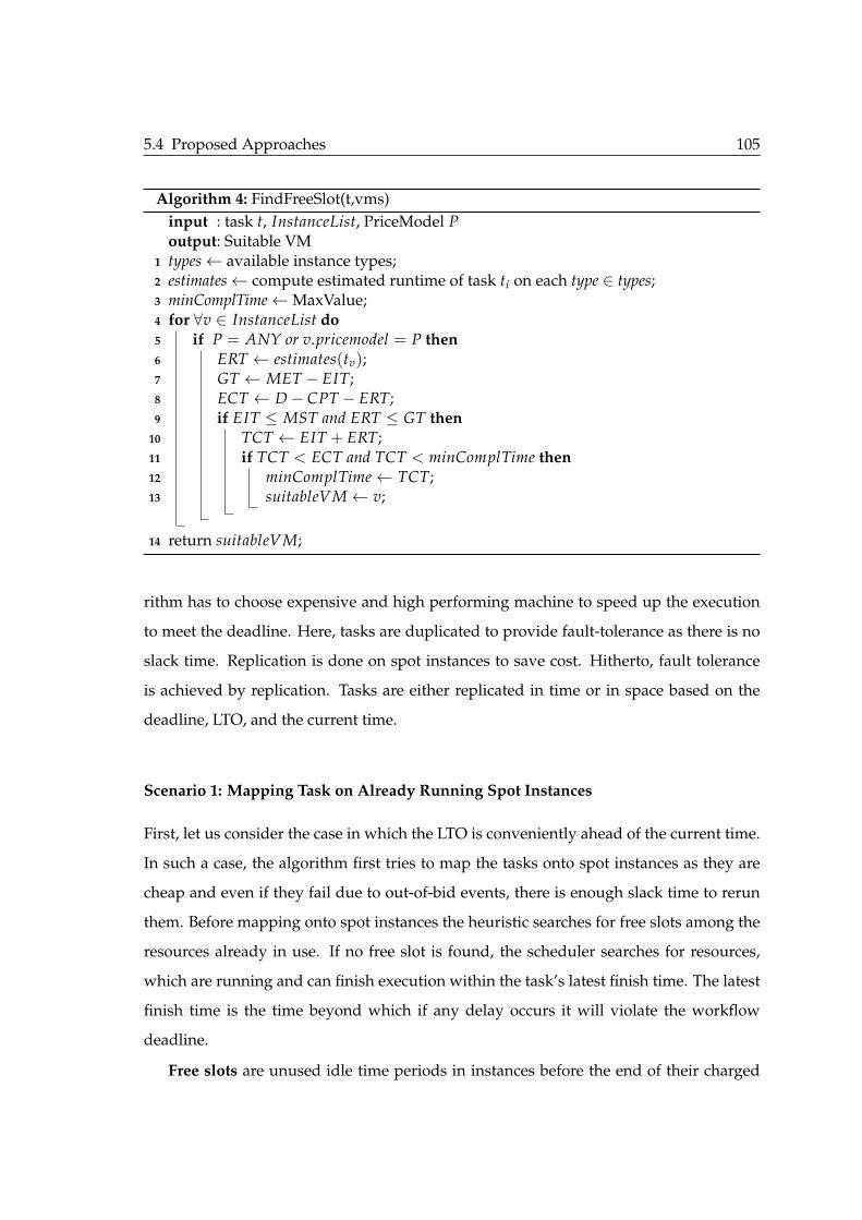
5.4 Proposed Approaches 105
Algorithm 4: FindFreeSlot(t,vms)input : task t, InstanceList, PriceModel Poutput: Suitable VM
1 types← available instance types;2 estimates← compute estimated runtime of task ti on each type ∈ types;3 minComplTime←MaxValue;4 for ∀v ∈ InstanceList do5 if P = ANY or v.pricemodel = P then6 ERT ← estimates(tv);7 GT ← MET − EIT;8 ECT ← D− CPT − ERT;9 if EIT ≤ MST and ERT ≤ GT then
10 TCT ← EIT + ERT;11 if TCT < ECT and TCT < minComplTime then12 minComplTime← TCT;13 suitableVM← v;
14 return suitableVM;
rithm has to choose expensive and high performing machine to speed up the execution
to meet the deadline. Here, tasks are duplicated to provide fault-tolerance as there is no
slack time. Replication is done on spot instances to save cost. Hitherto, fault tolerance
is achieved by replication. Tasks are either replicated in time or in space based on the
deadline, LTO, and the current time.
Scenario 1: Mapping Task on Already Running Spot Instances
First, let us consider the case in which the LTO is conveniently ahead of the current time.
In such a case, the algorithm first tries to map the tasks onto spot instances as they are
cheap and even if they fail due to out-of-bid events, there is enough slack time to rerun
them. Before mapping onto spot instances the heuristic searches for free slots among the
resources already in use. If no free slot is found, the scheduler searches for resources,
which are running and can finish execution within the task’s latest finish time. The latest
finish time is the time beyond which if any delay occurs it will violate the workflow
deadline.
Free slots are unused idle time periods in instances before the end of their charged
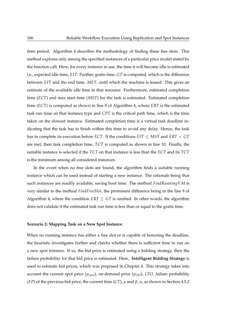
106 Reliable Workflow Execution Using Replication and Spot Instances
time period. Algorithm 4 describes the methodology of finding these free slots. This
method explores only among the specified instances of a particular price model stated by
the function call. Here, for every instance in use, the time it will become idle is estimated
i.e., expected idle time, EIT. Further, gratis time, GT is computed, which is the difference
between EIT and the end time, MET, until which the machine is leased. This gives an
estimate of the available idle time in that resource. Furthermore, estimated completion
time (ECT) and max start time (MST) for the task is estimated. Estimated completion
time (ECT) is computed as shown in line 8 of Algorithm 4, where ERT is the estimated
task run time on that instance type and CPT is the critical path time, which is the time
taken on the slowest instance. Estimated completion time is a virtual task deadline in-
dicating that the task has to finish within this time to avoid any delay. Hence, the task
has to complete its execution before ECT. If the conditions EIT ≤ MST and ERT < GT
are met, then task completion time, TCT is computed as shown in line 10. Finally, the
suitable instance is selected if the TCT on that instance is less than the ECT and its TCT
is the minimum among all considered instances.
In the event when no free slots are found, the algorithm finds a suitable running
instance which can be used instead of starting a new instance. The rationale being that
such instances are readily available, saving boot time. The method FindRunningVM is
very similar to the method FindFreeSlot, the prominent difference being in the line 9 of
Algorithm 4, where the condition ERT ≤ GT is omitted. In other words, the algorithm
does not validate if the estimated task run time is less than or equal to the gratis time.
Scenario 2: Mapping Task on a New Spot Instance
When no running instance has either a free slot or is capable of honoring the deadline,
the heuristic investigates further and checks whether there is sufficient time to run on
a new spot instance. If so, the bid price is estimated using a bidding strategy, then the
failure probability for that bid price is estimated. Here, Intelligent Bidding Strategy is
used to estimate bid prices, which was proposed in Chapter 4. This strategy takes into
account the current spot price (pspot), on-demand price (pOD), LTO, failure probability
(FP) of the previous bid price, the current time (CT), α and β. α, as shown in Section 4.5.2
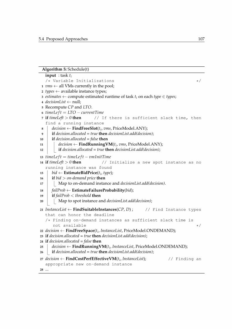
5.4 Proposed Approaches 107
Algorithm 5: Schedule(t)input : task ti/* Variable Initializations */
1 vms← all VMs currently in the pool;2 types← available instance types;3 estimates← compute estimated runtime of task ti on each type ∈ types;4 decisionList← null;5 Recompute CP and LTO.6 timeLe f t = LTO− currentTime7 if timeLeft > 0 then // If there is sufficient slack time, thenfind a running instance
8 decision← FindFreeSlot(ti, vms, PriceModel.ANY);9 if decision.allocated = true then decisionList.add(decision);
10 if decision.allocated = false then11 decision← FindRunningVM(ti, vms, PriceModel.ANY);12 if decision.allocated = true then decisionList.add(decision);
13 timeLe f t = timeLe f t− vmInitTime14 if timeLeft > 0 then // Initialize a new spot instance as no
running instance was found15 bid← EstimateBidPrice(ti, type);16 if bid > on-demand price then17 Map to on-demand instance and decisionList.add(decision).
18 failProb← EstimateFailureProbability(bid);19 if failProb < threshold then20 Map to spot instance and decisionList.add(decision);
21 InstanceList← FindSuitableInstances(CP, D) ; // Find Instance typesthat can honor the deadline/* Finding on-demand instances as sufficient slack time is
not available */22 decision← FindFreeSpace(ti, InstanceList, PriceModel.ONDEMAND);23 if decision.allocated = true then decisionList.add(decision);24 if decision.allocated = false then25 decision← FindRunningVM(ti, InstanceList, PriceModel.ONDEMAND);26 if decision.allocated = true then decisionList.add(decision);
27 decision← FindCostPerfEffectiveVM(ti, InstanceList); // Finding anappropriate new on-demand instance
28 ...
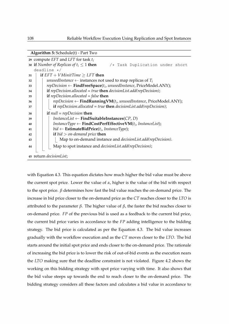
108 Reliable Workflow Execution Using Replication and Spot Instances
Algorithm 5: Schedule(t) - Part Two
29 compute EFT and LFT for task ti30 if Number of Replicas of ti ≤ 1 then /* Task Duplication under short
deadline */31 if EFT + VMinitTime ≥ LFT then32 unusedInstance← instances not used to map replicas of Ti33 repDecision← FindFreeSpace(ti, unusedInstance, PriceModel.ANY);34 if repDecision.allocated = true then decisionList.add(repDecision);35 if repDecision.allocated = false then36 repDecision← FindRunningVM(ti, unusedInstance, PriceModel.ANY);37 if repDecision.allocated = true then decisionList.add(repDecision);
38 if null = repDecision then39 InstanceList← FindSuitableInstances(CP, D)40 InstanceType← FindCostPerfEffectiveVM(ti, InstanceList);41 bid← EstimateBidPrice(ti, InstanceType);42 if bid > on-demand price then43 Map to on-demand instance and decisionList.add(repDecision).
44 Map to spot instance and decisionList.add(repDecision);
45 return decisionList;
with Equation 4.3. This equation dictates how much higher the bid value must be above
the current spot price. Lower the value of α, higher is the value of the bid with respect
to the spot price. β determines how fast the bid value reaches the on-demand price. The
increase in bid price closer to the on-demand price as the CT reaches closer to the LTO is
attributed to the parameter β. The higher value of β, the faster the bid reaches closer to
on-demand price. FP of the previous bid is used as a feedback to the current bid price,
the current bid price varies in accordance to the FP adding intelligence to the bidding
strategy. The bid price is calculated as per the Equation 4.3. The bid value increases
gradually with the workflow execution and as the CT moves closer to the LTO. The bid
starts around the initial spot price and ends closer to the on-demand price. The rationale
of increasing the bid price is to lower the risk of out-of-bid events as the execution nears
the LTO making sure that the deadline constraint is not violated. Figure 4.2 shows the
working on this bidding strategy with spot price varying with time. It also shows that
the bid value steeps up towards the end to reach closer to the on-demand price. The
bidding strategy considers all these factors and calculates a bid value in accordance to
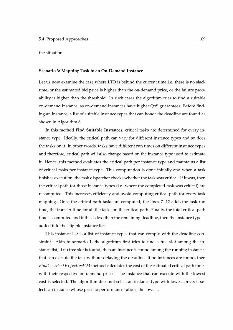
5.4 Proposed Approaches 109
the situation.
Scenario 3: Mapping Task to an On-Demand Instance
Let us now examine the case where LTO is behind the current time i.e. there is no slack
time, or the estimated bid price is higher than the on-demand price, or the failure prob-
ability is higher than the threshold. In such cases the algorithm tries to find a suitable
on-demand instance, as on-demand instances have higher QoS guarantees. Before find-
ing an instance, a list of suitable instance types that can honor the deadline are found as
shown in Algorithm 6.
In this method Find Suitable Instances, critical tasks are determined for every in-
stance type. Ideally, the critical path can vary for different instance types and so does
the tasks on it. In other words, tasks have different run times on different instance types
and therefore, critical path will also change based on the instance type used to estimate
it. Hence, this method evaluates the critical path per instance type and maintains a list
of critical tasks per instance type. This computation is done initially and when a task
finishes execution, the task dispatcher checks whether the task was critical. If it was, then
the critical path for those instance types (i.e. where the completed task was critical) are
recomputed. This increases efficiency and avoid computing critical path for every task
mapping. Once the critical path tasks are computed, the lines 7- 12 adds the task run
time, the transfer time for all the tasks on the critical path. Finally, the total critical path
time is computed and if this is less than the remaining deadline, then the instance type is
added into the eligible instance list.
This instance list is a list of instance types that can comply with the deadline con-
straint. Akin to scenario 1, the algorithm first tries to find a free slot among the in-
stance list, if no free slot is found, then an instance is found among the running instances
that can execute the task without delaying the deadline. If no instances are found, then
FindCostPer f E f f ectiveVM method calculates the cost of the estimated critical path times
with their respective on-demand prices. The instance that can execute with the lowest
cost is selected. The algorithm does not select an instance type with lowest price; it se-
lects an instance whose price to performance ratio is the lowest.

110 Reliable Workflow Execution Using Replication and Spot Instances
Algorithm 6: FindSuitableInstances(estimates)input : estimatesoutput: Eligible Instance List
1 types← available instance types;2 InstanceList← null3 for ∀i ∈ InstanceTypes do4 CPTasks← computeCPTasks(i);5 prevTask← null;6 CPTime← 0;7 for ∀t ∈ CPTasks do8 if prevTask 6= null then9 edgeTime← edgeTime(prevTask, t);
10 CPTime+ = estimates(t) + edgeTime;11 prevTime← t;
12 totalCPTime = CPTime + VMInitTime;13 if totalCPTime ≤ D− currenttime then14 InstanceList.add(i);
15 return InstanceList;
Scenario 4: Task Duplication Under Short Deadline
Critical tasks are replicated to provide fault tolerance when the deadline is short. We pro-
pose two variants of this heuristic. The two heuristics are very similar, with the difference
being the tasks they replicate.
Essential Critical Path Task Replication (ECPTR) heuristic: The algorithm 5 de-
tails its working. Here, when the LTO has passed the current time, and the task has
no slack time, then a replica is created. In other words, all ESCTs are replicated. Simi-
lar to the scenarios presented before, first free slots are found among the instances that
have not been used to map the replicas of the task considered. If no free slots are found,
then a running instance is found that can be used to the map the task without violat-
ing the deadline. When neither free slots nor running instances are found, the heuristic
maps the replica onto a spot instance. The type of spot instance is decided by methods
FindSuitableInstances and FindCostPer f E f f ectiveVM as shown in lines 39 to 40. Finally,
using the bidding strategy, a bid price is estimated for the spot price and if this bid price
is less than the on-demand price then a spot instance is instantiated mapping the replica
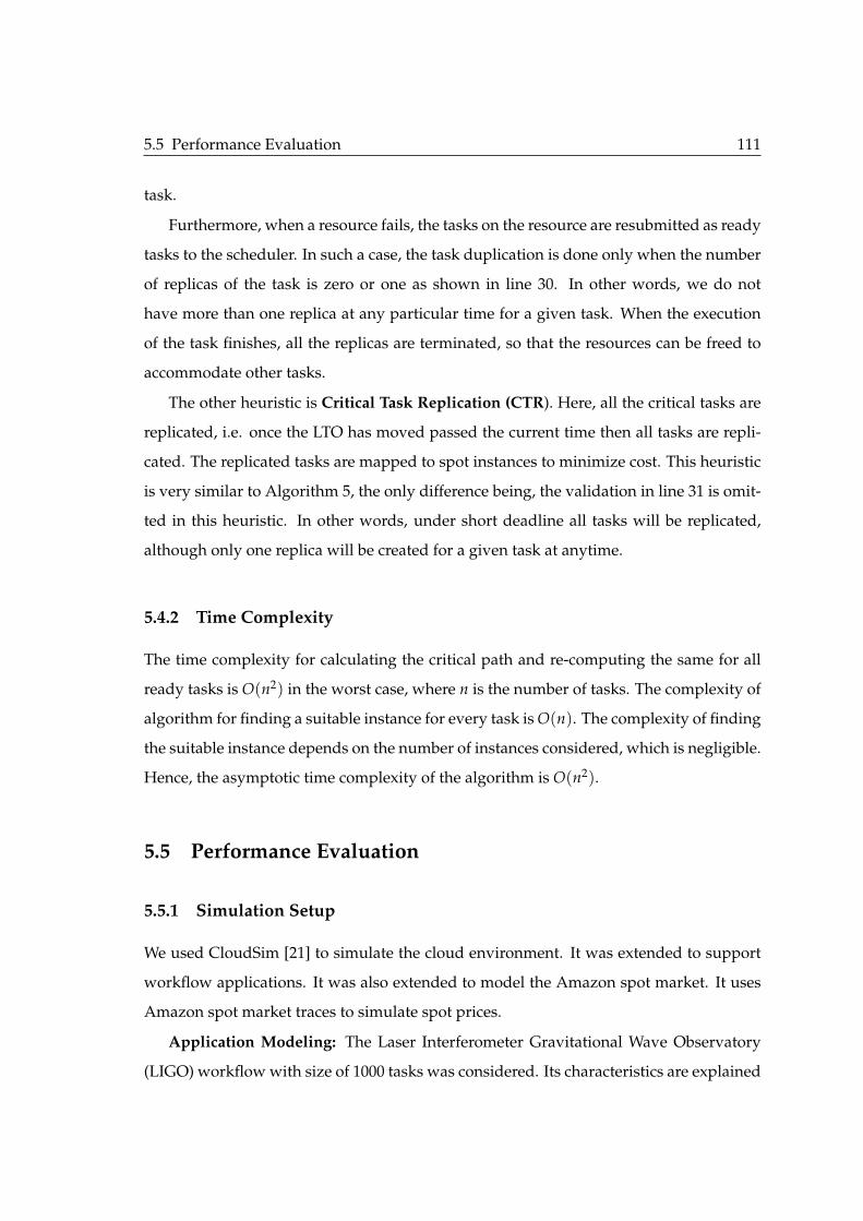
5.5 Performance Evaluation 111
task.
Furthermore, when a resource fails, the tasks on the resource are resubmitted as ready
tasks to the scheduler. In such a case, the task duplication is done only when the number
of replicas of the task is zero or one as shown in line 30. In other words, we do not
have more than one replica at any particular time for a given task. When the execution
of the task finishes, all the replicas are terminated, so that the resources can be freed to
accommodate other tasks.
The other heuristic is Critical Task Replication (CTR). Here, all the critical tasks are
replicated, i.e. once the LTO has moved passed the current time then all tasks are repli-
cated. The replicated tasks are mapped to spot instances to minimize cost. This heuristic
is very similar to Algorithm 5, the only difference being, the validation in line 31 is omit-
ted in this heuristic. In other words, under short deadline all tasks will be replicated,
although only one replica will be created for a given task at anytime.
5.4.2 Time Complexity
The time complexity for calculating the critical path and re-computing the same for all
ready tasks is O(n2) in the worst case, where n is the number of tasks. The complexity of
algorithm for finding a suitable instance for every task is O(n). The complexity of finding
the suitable instance depends on the number of instances considered, which is negligible.
Hence, the asymptotic time complexity of the algorithm is O(n2).
5.5 Performance Evaluation
5.5.1 Simulation Setup
We used CloudSim [21] to simulate the cloud environment. It was extended to support
workflow applications. It was also extended to model the Amazon spot market. It uses
Amazon spot market traces to simulate spot prices.
Application Modeling: The Laser Interferometer Gravitational Wave Observatory
(LIGO) workflow with size of 1000 tasks was considered. Its characteristics are explained
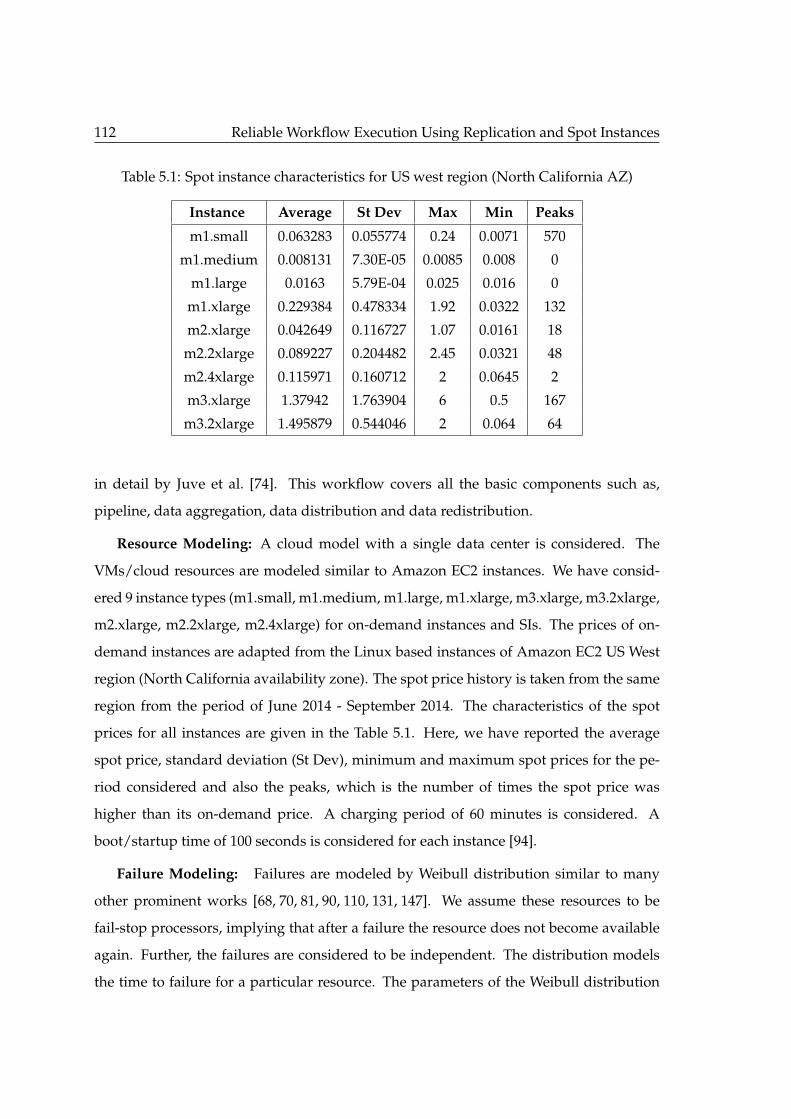
112 Reliable Workflow Execution Using Replication and Spot Instances
Table 5.1: Spot instance characteristics for US west region (North California AZ)
Instance Average St Dev Max Min Peaks
m1.small 0.063283 0.055774 0.24 0.0071 570
m1.medium 0.008131 7.30E-05 0.0085 0.008 0
m1.large 0.0163 5.79E-04 0.025 0.016 0
m1.xlarge 0.229384 0.478334 1.92 0.0322 132
m2.xlarge 0.042649 0.116727 1.07 0.0161 18
m2.2xlarge 0.089227 0.204482 2.45 0.0321 48
m2.4xlarge 0.115971 0.160712 2 0.0645 2
m3.xlarge 1.37942 1.763904 6 0.5 167
m3.2xlarge 1.495879 0.544046 2 0.064 64
in detail by Juve et al. [74]. This workflow covers all the basic components such as,
pipeline, data aggregation, data distribution and data redistribution.
Resource Modeling: A cloud model with a single data center is considered. The
VMs/cloud resources are modeled similar to Amazon EC2 instances. We have consid-
ered 9 instance types (m1.small, m1.medium, m1.large, m1.xlarge, m3.xlarge, m3.2xlarge,
m2.xlarge, m2.2xlarge, m2.4xlarge) for on-demand instances and SIs. The prices of on-
demand instances are adapted from the Linux based instances of Amazon EC2 US West
region (North California availability zone). The spot price history is taken from the same
region from the period of June 2014 - September 2014. The characteristics of the spot
prices for all instances are given in the Table 5.1. Here, we have reported the average
spot price, standard deviation (St Dev), minimum and maximum spot prices for the pe-
riod considered and also the peaks, which is the number of times the spot price was
higher than its on-demand price. A charging period of 60 minutes is considered. A
boot/startup time of 100 seconds is considered for each instance [94].
Failure Modeling: Failures are modeled by Weibull distribution similar to many
other prominent works [68, 70, 81, 90, 110, 131, 147]. We assume these resources to be
fail-stop processors, implying that after a failure the resource does not become available
again. Further, the failures are considered to be independent. The distribution models
the time to failure for a particular resource. The parameters of the Weibull distribution
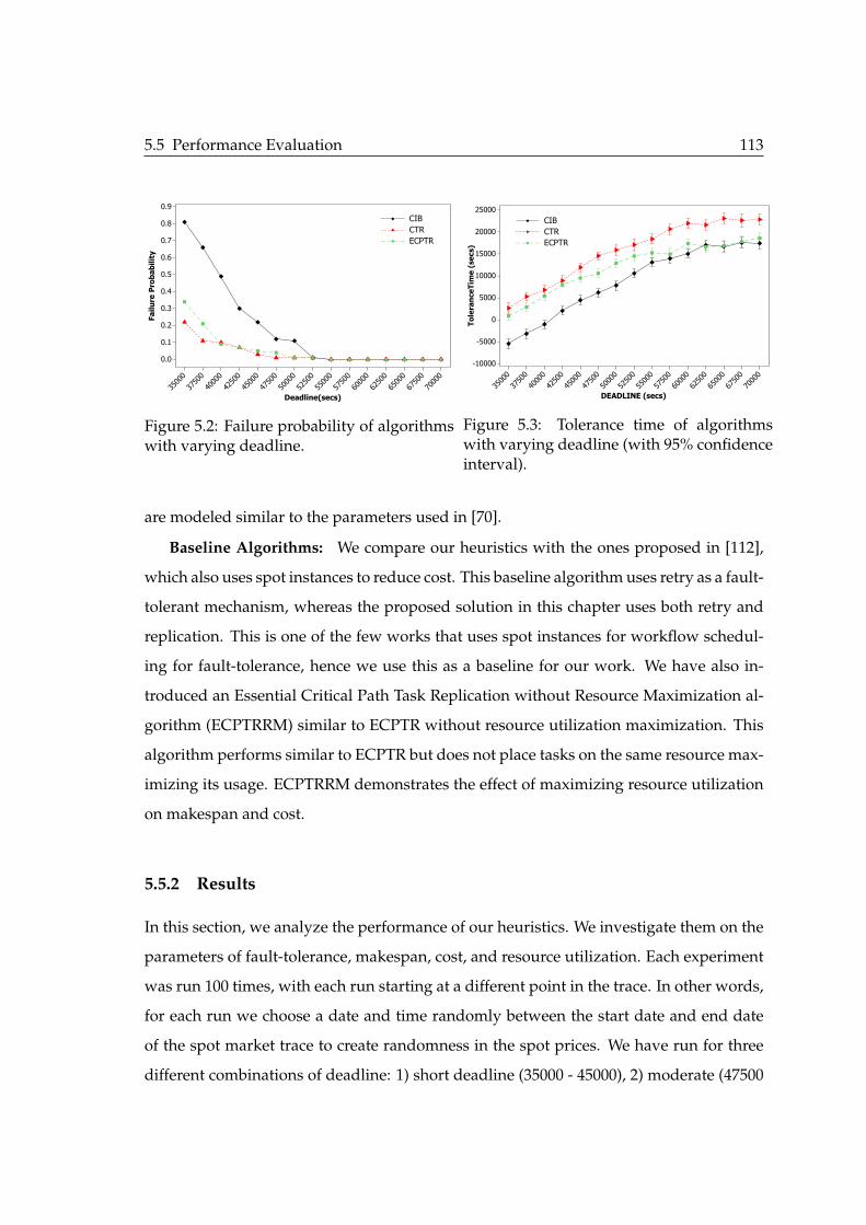
5.5 Performance Evaluation 113
70000
67500
65000
62500
60000
57500
55000
52500
50000
47500
45000
42500
40000
37500
35000
0.9
0.8
0.7
0.6
0.5
0.4
0.3
0.2
0.1
0.0
Deadline(secs)
Failure Probability
CIB
CTR
ECPTR
Figure 5.2: Failure probability of algorithmswith varying deadline.
70000
67500
65000
62500
60000
57500
55000
52500
50000
47500
45000
42500
40000
37500
35000
25000
20000
15000
10000
5000
0
-5000
-10000
ToleranceTime (secs)
CIB
CTR
ECPTR
DEADLINE (secs)
Figure 5.3: Tolerance time of algorithmswith varying deadline (with 95% confidenceinterval).
are modeled similar to the parameters used in [70].
Baseline Algorithms: We compare our heuristics with the ones proposed in [112],
which also uses spot instances to reduce cost. This baseline algorithm uses retry as a fault-
tolerant mechanism, whereas the proposed solution in this chapter uses both retry and
replication. This is one of the few works that uses spot instances for workflow schedul-
ing for fault-tolerance, hence we use this as a baseline for our work. We have also in-
troduced an Essential Critical Path Task Replication without Resource Maximization al-
gorithm (ECPTRRM) similar to ECPTR without resource utilization maximization. This
algorithm performs similar to ECPTR but does not place tasks on the same resource max-
imizing its usage. ECPTRRM demonstrates the effect of maximizing resource utilization
on makespan and cost.
5.5.2 Results
In this section, we analyze the performance of our heuristics. We investigate them on the
parameters of fault-tolerance, makespan, cost, and resource utilization. Each experiment
was run 100 times, with each run starting at a different point in the trace. In other words,
for each run we choose a date and time randomly between the start date and end date
of the spot market trace to create randomness in the spot prices. We have run for three
different combinations of deadline: 1) short deadline (35000 - 45000), 2) moderate (47500
114 Reliable Workflow Execution Using Replication and Spot Instances
- 57500) and 3) relaxed deadline (60000 - 70000) as shown in the Figures 5.2-5.8. Next, we
present results and their analysis on the performance of our heuristics with regards to
different parameters.
Fault Tolerance
Providing fault-tolerant schedules is the main objective of this proposed algorithm. Fig-
ures 5.2 and 5.3 show the performance of our heuristics with respect to two metrics,
failure probability and tolerance time. The details of the metrics were mentioned earlier
in section 5.3.
The failure probabilities of the different algorithms are shown in Figure 5.2. It can
be observed that under relaxed deadline, all algorithms have substantially lower failure
probabilities. When the deadline is short, it can be observed that the heuristics CTR and
ECPTR perform considerably better than the baseline CIB. Failure probability of CTR
and ECPTR are lower than CIB by 79.75% and 72.36% respectively on average under
short deadlines. This is a strong indication that our heuristics have a high probability of
success in spite of failures in the environment.
Figure 5.3 depicts the results with respect to the tolerance time. It can be observed
that the baseline algorithm CIB has negative tolerance time under short deadlines. This
implies that CIB algorithm is not fault-tolerant under short deadline, whereas on the
other hand both the proposed heuristics CTR and ECPTR have significantly positive tol-
erance time. This suggests that they are fault-tolerant and can withstand more failures
and performance variations given the same schedule. It is also evident from the figure
that ECPTR has a higher tolerance time than CTR and this difference becomes larger
as the deadline becomes relaxed. Additionally, the tolerance time of CIB and ECPTR
become similar as the deadline is relaxed. This is due to the fact that CIB and ECPTR
perform similar to each other under relaxed deadlines.
Effect on Makespan
Makespan is the other important objective that we consider. We attempt to minimize
it especially when the deadline is short. Figures 5.4 and 5.5 are presented, showing the
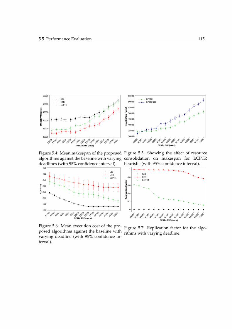
5.5 Performance Evaluation 115
70000
67500
65000
62500
60000
57500
55000
52500
50000
47500
45000
42500
40000
37500
35000
55000
50000
45000
40000
35000
30000
MAKESPAN (secs)
CIB
CTR
ECPTR
DEADLINE (secs)
Figure 5.4: Mean makespan of the proposedalgorithms against the baseline with varyingdeadlines (with 95% confidence interval).
70000
67500
65000
62500
60000
57500
55000
52500
50000
47500
45000
42500
40000
37500
35000
65000
60000
55000
50000
45000
40000
35000
30000
MAKESPAN (secs)
ECPTR
ECPTRRM
DEADLINE (secs)
Figure 5.5: Showing the effect of resourceconsolidation on makespan for ECPTRheuristic (with 95% confidence interval).
70000
67500
65000
62500
60000
57500
55000
52500
50000
47500
45000
42500
40000
37500
35000
450
400
350
300
250
200
150
100
COST ($)
CIB
CTR
ECPTR
DEADLINE (secs)
Figure 5.6: Mean execution cost of the pro-posed algorithms against the baseline withvarying deadline (with 95% confidence in-terval).
70000
67500
65000
62500
60000
57500
55000
52500
50000
47500
45000
42500
40000
37500
35000
1
0.8
0.6
0.4
0.2
0
DEADLINE (secs)
Replication Factor
CIB
CTR
ECPTR
Figure 5.7: Replication factor for the algo-rithms with varying deadline.
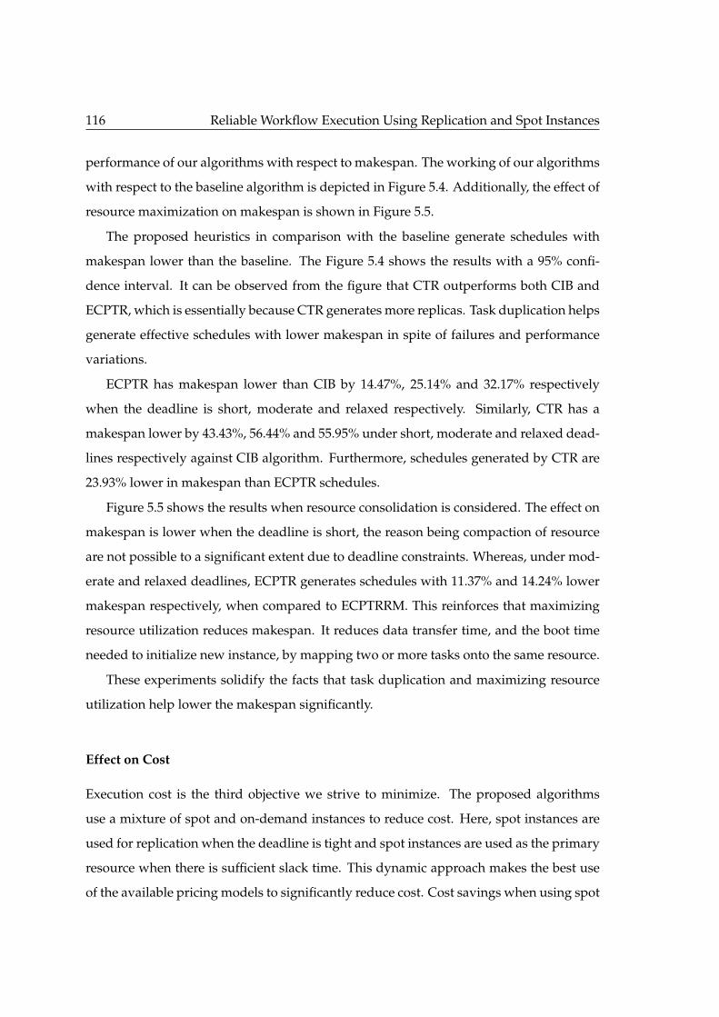
116 Reliable Workflow Execution Using Replication and Spot Instances
performance of our algorithms with respect to makespan. The working of our algorithms
with respect to the baseline algorithm is depicted in Figure 5.4. Additionally, the effect of
resource maximization on makespan is shown in Figure 5.5.
The proposed heuristics in comparison with the baseline generate schedules with
makespan lower than the baseline. The Figure 5.4 shows the results with a 95% confi-
dence interval. It can be observed from the figure that CTR outperforms both CIB and
ECPTR, which is essentially because CTR generates more replicas. Task duplication helps
generate effective schedules with lower makespan in spite of failures and performance
variations.
ECPTR has makespan lower than CIB by 14.47%, 25.14% and 32.17% respectively
when the deadline is short, moderate and relaxed respectively. Similarly, CTR has a
makespan lower by 43.43%, 56.44% and 55.95% under short, moderate and relaxed dead-
lines respectively against CIB algorithm. Furthermore, schedules generated by CTR are
23.93% lower in makespan than ECPTR schedules.
Figure 5.5 shows the results when resource consolidation is considered. The effect on
makespan is lower when the deadline is short, the reason being compaction of resource
are not possible to a significant extent due to deadline constraints. Whereas, under mod-
erate and relaxed deadlines, ECPTR generates schedules with 11.37% and 14.24% lower
makespan respectively, when compared to ECPTRRM. This reinforces that maximizing
resource utilization reduces makespan. It reduces data transfer time, and the boot time
needed to initialize new instance, by mapping two or more tasks onto the same resource.
These experiments solidify the facts that task duplication and maximizing resource
utilization help lower the makespan significantly.
Effect on Cost
Execution cost is the third objective we strive to minimize. The proposed algorithms
use a mixture of spot and on-demand instances to reduce cost. Here, spot instances are
used for replication when the deadline is tight and spot instances are used as the primary
resource when there is sufficient slack time. This dynamic approach makes the best use
of the available pricing models to significantly reduce cost. Cost savings when using spot
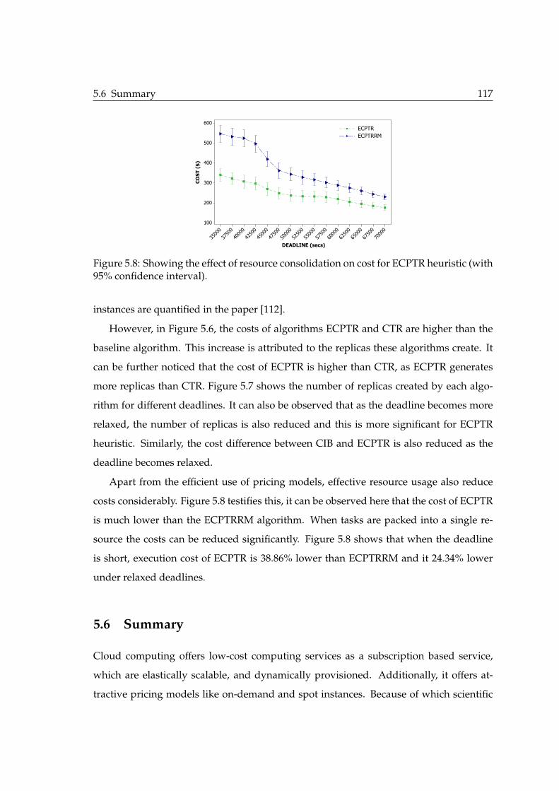
5.6 Summary 117
70000
67500
65000
62500
60000
57500
55000
52500
50000
47500
45000
42500
40000
37500
35000
600
500
400
300
200
100
COST ($)
ECPTR
ECPTRRM
DEADLINE (secs)
Figure 5.8: Showing the effect of resource consolidation on cost for ECPTR heuristic (with95% confidence interval).
instances are quantified in the paper [112].
However, in Figure 5.6, the costs of algorithms ECPTR and CTR are higher than the
baseline algorithm. This increase is attributed to the replicas these algorithms create. It
can be further noticed that the cost of ECPTR is higher than CTR, as ECPTR generates
more replicas than CTR. Figure 5.7 shows the number of replicas created by each algo-
rithm for different deadlines. It can also be observed that as the deadline becomes more
relaxed, the number of replicas is also reduced and this is more significant for ECPTR
heuristic. Similarly, the cost difference between CIB and ECPTR is also reduced as the
deadline becomes relaxed.
Apart from the efficient use of pricing models, effective resource usage also reduce
costs considerably. Figure 5.8 testifies this, it can be observed here that the cost of ECPTR
is much lower than the ECPTRRM algorithm. When tasks are packed into a single re-
source the costs can be reduced significantly. Figure 5.8 shows that when the deadline
is short, execution cost of ECPTR is 38.86% lower than ECPTRRM and it 24.34% lower
under relaxed deadlines.
5.6 Summary
Cloud computing offers low-cost computing services as a subscription based service,
which are elastically scalable, and dynamically provisioned. Additionally, it offers at-
tractive pricing models like on-demand and spot instances. Because of which scientific

118 Reliable Workflow Execution Using Replication and Spot Instances
workflow management systems are rapidly moving towards clouds.
However, cloud environments are prone to failures and performance variations
among resources. Failures are traditionally mitigated using replication, which increases
the execution cost and time. Whereas with innovative pricing models cloud offers, the
cost for providing fault-tolerance can be drastically reduced. In this chapter, we have
proposed two just-in-time adaptive workflow scheduling heuristics for clouds. These
heuristics use on-demand and spot instances to provide fault-tolerant schedules whilst
minimizing time and cost. They are fault-tolerant against performance variations, out-
of-bid failures and resource failures. Extensive simulations have shown that the pro-
posed heuristics generate schedules with significantly lower failure probabilities. The
makespan of these schedules is much lower than the baseline algorithm. These heuristics
are also shown to maximize resource utilization. These experiments establish that pricing
models offered by cloud providers can be used to reduce costs and makespan and at the
same time provide robust and resilient schedules.
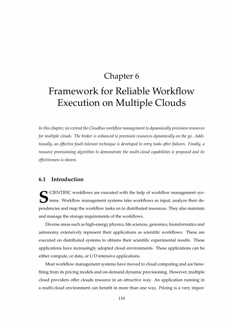
Chapter 6
Framework for Reliable WorkflowExecution on Multiple Clouds
In this chapter, we extend the Cloudbus workflow management to dynamically provision resources
for multiple clouds. The broker is enhanced to provision resources dynamically on the go. Addi-
tionally, an effective fault-tolerant technique is developed to retry tasks after failures. Finally, a
resource provisioning algorithm to demonstrate the multi-cloud capabilities is proposed and its
effectiveness is shown.
6.1 Introduction
SCIENTIFIC workflows are executed with the help of workflow management sys-
tems. Workflow management systems take workflows as input, analyze their de-
pendencies and map the workflow tasks on to distributed resources. They also maintain
and manage the storage requirements of the workflows.
Diverse areas such as high-energy physics, life sciences, genomics, bioinformatics and
astronomy extensively represent their applications as scientific workflows. These are
executed on distributed systems to obtains their scientific experimental results. These
applications have increasingly adopted cloud environments. These applications can be
either compute, or data, or I/O intensive applications.
Most workflow management systems have moved to cloud computing and are bene-
fiting from its pricing models and on-demand dynamic provisioning. However, multiple
cloud providers offer clouds resource in an attractive way. An application running in
a multi-cloud environment can benefit in more than one way. Pricing is a very impor-
119
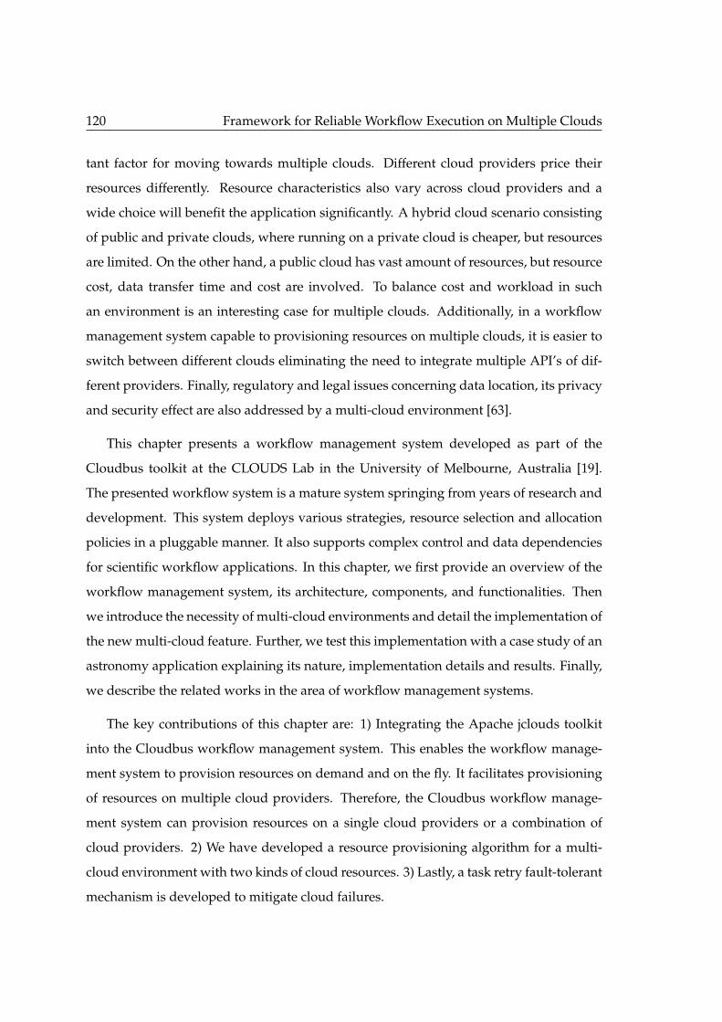
120 Framework for Reliable Workflow Execution on Multiple Clouds
tant factor for moving towards multiple clouds. Different cloud providers price their
resources differently. Resource characteristics also vary across cloud providers and a
wide choice will benefit the application significantly. A hybrid cloud scenario consisting
of public and private clouds, where running on a private cloud is cheaper, but resources
are limited. On the other hand, a public cloud has vast amount of resources, but resource
cost, data transfer time and cost are involved. To balance cost and workload in such
an environment is an interesting case for multiple clouds. Additionally, in a workflow
management system capable to provisioning resources on multiple clouds, it is easier to
switch between different clouds eliminating the need to integrate multiple API’s of dif-
ferent providers. Finally, regulatory and legal issues concerning data location, its privacy
and security effect are also addressed by a multi-cloud environment [63].
This chapter presents a workflow management system developed as part of the
Cloudbus toolkit at the CLOUDS Lab in the University of Melbourne, Australia [19].
The presented workflow system is a mature system springing from years of research and
development. This system deploys various strategies, resource selection and allocation
policies in a pluggable manner. It also supports complex control and data dependencies
for scientific workflow applications. In this chapter, we first provide an overview of the
workflow management system, its architecture, components, and functionalities. Then
we introduce the necessity of multi-cloud environments and detail the implementation of
the new multi-cloud feature. Further, we test this implementation with a case study of an
astronomy application explaining its nature, implementation details and results. Finally,
we describe the related works in the area of workflow management systems.
The key contributions of this chapter are: 1) Integrating the Apache jclouds toolkit
into the Cloudbus workflow management system. This enables the workflow manage-
ment system to provision resources on demand and on the fly. It facilitates provisioning
of resources on multiple cloud providers. Therefore, the Cloudbus workflow manage-
ment system can provision resources on a single cloud providers or a combination of
cloud providers. 2) We have developed a resource provisioning algorithm for a multi-
cloud environment with two kinds of cloud resources. 3) Lastly, a task retry fault-tolerant
mechanism is developed to mitigate cloud failures.
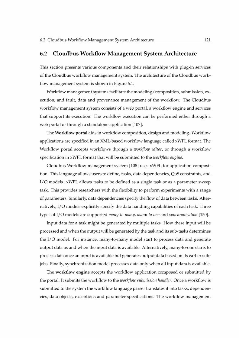
6.2 Cloudbus Workflow Management System Architecture 121
6.2 Cloudbus Workflow Management System Architecture
This section presents various components and their relationships with plug-in services
of the Cloudbus workflow management system. The architecture of the Cloudbus work-
flow management system is shown in Figure 6.1.
Workflow management systems facilitate the modeling/composition, submission, ex-
ecution, and fault, data and provenance management of the workflow. The Cloudbus
workflow management system consists of a web portal, a workflow engine and services
that support its execution. The workflow execution can be performed either through a
web portal or through a standalone application [107].
The Workflow portal aids in workflow composition, design and modeling. Workflow
applications are specified in an XML-based workflow language called xWFL format. The
Workflow portal accepts workflows through a workflow editor, or through a workflow
specification in xWFL format that will be submitted to the workflow engine.
Cloudbus Workflow management system [108] uses xWFL for application composi-
tion. This language allows users to define, tasks, data dependencies, QoS constraints, and
I/O models. xWFL allows tasks to be defined as a single task or as a parameter sweep
task. This provides researchers with the flexibility to perform experiments with a range
of parameters. Similarly, data dependencies specify the flow of data between tasks. Alter-
natively, I/O models explicitly specify the data handling capabilities of each task. Three
types of I/O models are supported many-to-many, many-to-one and synchronization [150].
Input data for a task might be generated by multiple tasks. How these input will be
processed and when the output will be generated by the task and its sub-tasks determines
the I/O model. For instance, many-to-many model start to process data and generate
output data as and when the input data is available. Alternatively, many-to-one starts to
process data once an input is available but generates output data based on its earlier sub-
jobs. Finally, synchronization model processes data only when all input data is available.
The workflow engine accepts the workflow application composed or submitted by
the portal. It submits the workflow to the workflow submission handler. Once a workflow is
submitted to the system the workflow language parser translates it into tasks, dependen-
cies, data objects, exceptions and parameter specifications. The workflow management
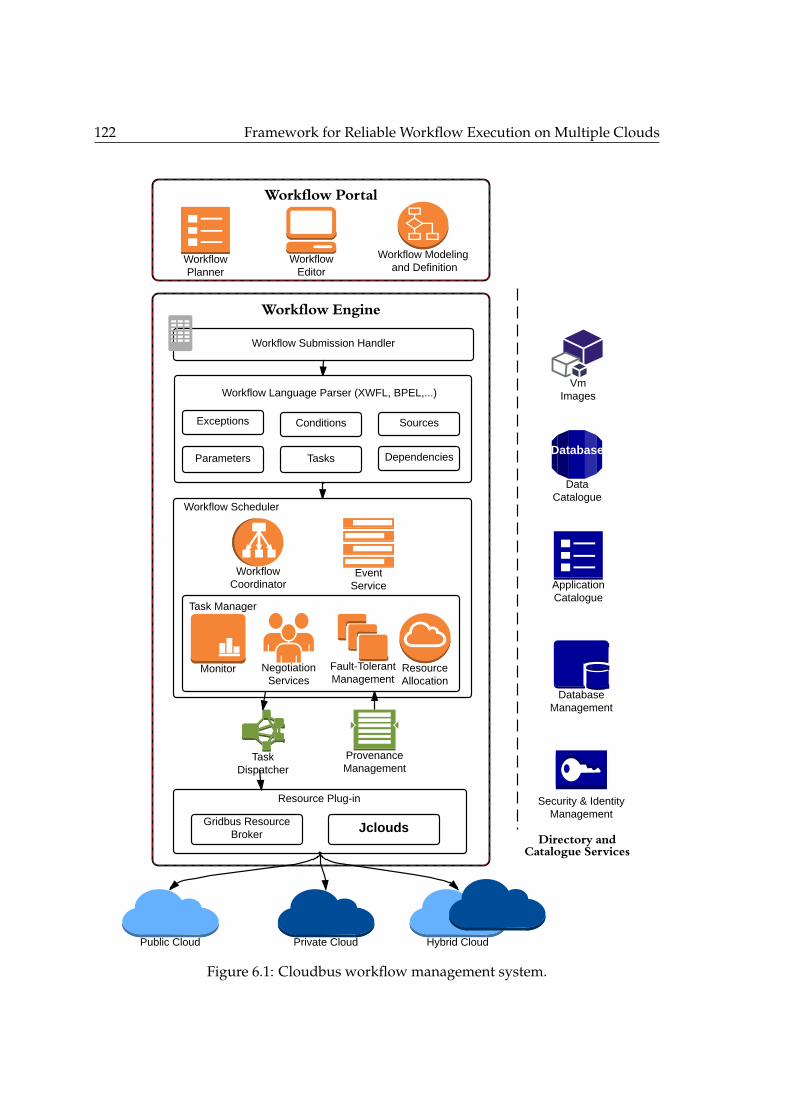
122 Framework for Reliable Workflow Execution on Multiple Clouds
Task Dispatcher
Fault-Tolerant Management
Resource Allocation
Workflow Engine
Public Cloud
Cloud
Workflow Editor
Workflow Modeling and Definition
Database Management
Workflow Coordinator
Negotiation Services
Provenance Management
Vm Images
Application Catalogue
Data Catalogue
Database
Workflow Por tal
D irectory andCatalogue Services
Hybrid CloudPrivate Cloud
Security & Identity Management
Workflow Planner
Workflow Submission Handler
Workflow Language Parser (XWFL, BPEL,...)
Parameters Dependencies
SourcesConditionsExceptions
Tasks
Event Service
Workflow Scheduler
Monitor
Task Manager
Resource Plug-in
Gridbus Resource Broker Jclouds
Figure 6.1: Cloudbus workflow management system.
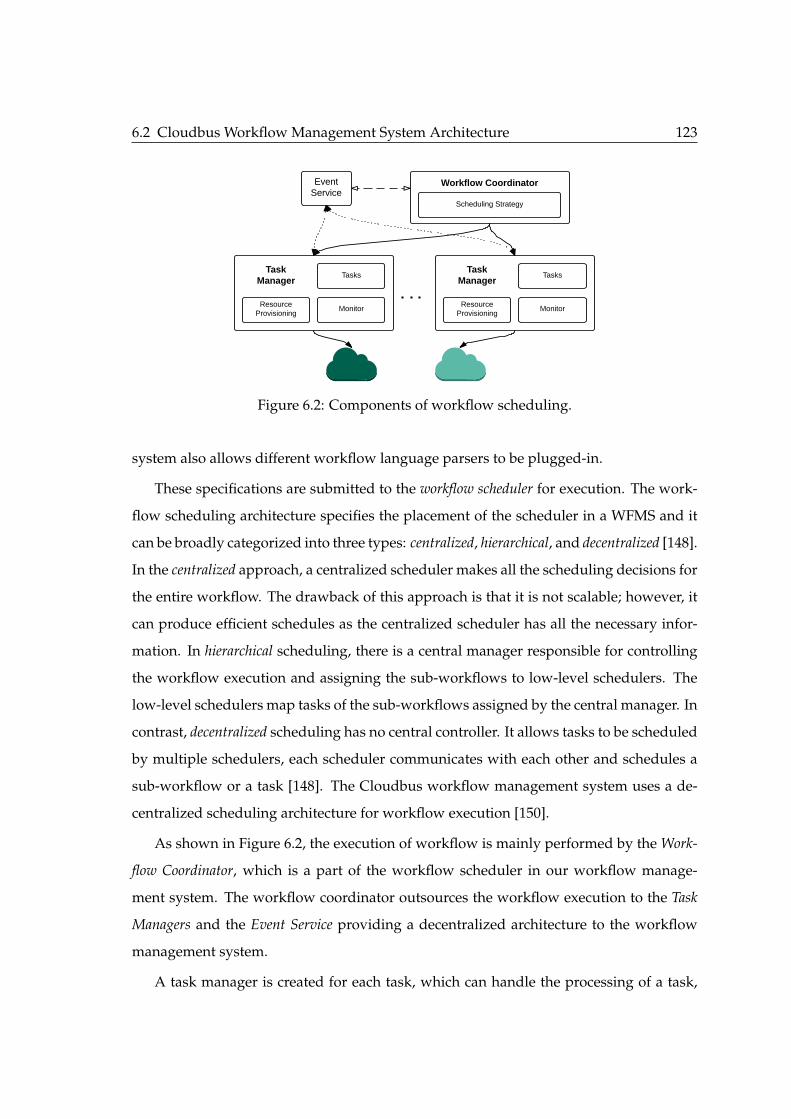
6.2 Cloudbus Workflow Management System Architecture 123
EventService
Scheduling Strategy
Workflow Coordinator
Tasks
MonitorResourceProvisioning
TaskManager
Tasks
MonitorResourceProvisioning
TaskManager
Figure 6.2: Components of workflow scheduling.
system also allows different workflow language parsers to be plugged-in.
These specifications are submitted to the workflow scheduler for execution. The work-
flow scheduling architecture specifies the placement of the scheduler in a WFMS and it
can be broadly categorized into three types: centralized, hierarchical, and decentralized [148].
In the centralized approach, a centralized scheduler makes all the scheduling decisions for
the entire workflow. The drawback of this approach is that it is not scalable; however, it
can produce efficient schedules as the centralized scheduler has all the necessary infor-
mation. In hierarchical scheduling, there is a central manager responsible for controlling
the workflow execution and assigning the sub-workflows to low-level schedulers. The
low-level schedulers map tasks of the sub-workflows assigned by the central manager. In
contrast, decentralized scheduling has no central controller. It allows tasks to be scheduled
by multiple schedulers, each scheduler communicates with each other and schedules a
sub-workflow or a task [148]. The Cloudbus workflow management system uses a de-
centralized scheduling architecture for workflow execution [150].
As shown in Figure 6.2, the execution of workflow is mainly performed by the Work-
flow Coordinator, which is a part of the workflow scheduler in our workflow manage-
ment system. The workflow coordinator outsources the workflow execution to the Task
Managers and the Event Service providing a decentralized architecture to the workflow
management system.
A task manager is created for each task, which can handle the processing of a task,
124 Framework for Reliable Workflow Execution on Multiple Clouds
including resource allocation and discovery, monitoring, negotiation services, and fault-
tolerant management. Each task manager employs their own strategies for resource pro-
visioning, SLA and data management. They also have monitors to monitor the task exe-
cution status on a cloud resource. As shown in the Figure 6.2, each task has its own task
manager.
Additionally, two fault handling techniques are available and they are retry and task
replication [150]. Retry mechanism reschedules a failed job to an available resource. It
also records the number of failed jobs for each resource. A warning threshold is set for
the number of failed jobs on a particular resource, and if this threshold is exceeded the
scheduler decreases the quantum of jobs submitted to this resource. However, if the
number of failed jobs exceeds a critical threshold, then the scheduler stops submitting
jobs to that resource.
The task replication technique replicates a task on more than one resource. The earli-
est resource to produce the output is used. These two mechanisms help mitigate failures
and performance variations that can be experienced in distributed environments.
To manage the entire workflow execution coherently, there is a necessity for a com-
munication model, as every task manager is an independent and parallel thread for task
execution. However, these tasks managers are dependent on other tasks through data
and/or control dependencies and these dependencies could be one-to-one or many-to-
many.
Event service addresses this requirement by providing an event-driven mechanism
with subscription-notification model to control and manage execution activities. This ser-
vice registers events from tasks managers and notifies the workflow coordinator. There-
fore, task managers do not communicate with each other, making the event service a
loosely coupled design allowing new and easily pluggable extension into the architec-
ture.
Event services allow three types of events basically: status event, output events and con-
trol events. Task managers send status and output events informing about their execution
statuses and results. Workflow coordinator sends control events to task managers, such
as pause and resume.
6.3 Multi-Cloud Framework for Cloudbus Workflow Engine 125
Once the workflow scheduler maps a task to a resource, the dispatcher dispatches the
tasks to the right middleware. The workflow management system is designed to support
multiple middleware and this is done by creating dispatchers for each middleware. The
dispatcher supports interaction with resources of a specific kind. Currently, the Cloudbus
WFMS supports Aneka, Globus, and fork-based middleware.
Plug-ins supports various services that aid in workflow execution on different envi-
ronments and platforms. The workflow management system has several plug-ins for:
• Determining task, data, and resources characteristics through metadata informa-
tion or through trace files.
• Data transfer between broker, resources and storage.
• Monitoring the status of tasks, application, and resources.
• Catalogues services for resources, tasks, and their replicas.
6.3 Multi-Cloud Framework for Cloudbus Workflow Engine
Workflow management systems have migrated in huge numbers from grids to clouds.
Multiple large software companies have ventured into the cloud domain offering cloud
resources with innovative and attractive pricing and other benefits. To leverage these fea-
tures from multiple cloud providers, its imperative that existing workflow management
system evolve to work in a multi-cloud environment and not be locked in to a single
cloud provider.
Advantages of a multi-cloud environment are manifold: 1) Pricing: multiple cloud
providers offer cloud resources through various pricing models. For example, AWS offer
spot instances which are very cheap but have lower SLAs guarantee. Similarly, there are
reserved instances, and on-demand instances, and each pricing model has its pros and
cons. 2) Billing Periods: cloud providers provision cloud resources with different billing
periods, for example, AWS bills resources per hour, Google bills per minute. Depending
on the workflow task length, choosing the right billing period can increase cost savings
significantly. 3) Resource characteristics: cloud providers offer resources with different
126 Framework for Reliable Workflow Execution on Multiple Clouds
characteristics with varying RAM, CPU and others, this enables the workflow manage-
ment system to pick the right configuration for a task based on whether it is compute
intensive, data intensive, or I/O intensive. 4) Private cloud: many organization and in-
stitutes have private clouds, where computation is generally free. However, resources
are limited in such an environment and a combination of private and public cloud in-
frastructures could address these resource limitations. 5) Regulatory and legal: issues con-
cerning data location, its privacy and security affect in choosing an appropriate cloud
provider [63].
Multi-cloud frameworks address all these issues and help large and complex work-
flows to execute seamlessly. However, moving to multi-cloud environment has its own
challenges. Latency between users and different clouds could impact the application
performance largely. Cloud providers do not have similar API’s for accessing their cloud
infrastructures. Therefore, interoperability is a major issue. Additionally, time and cost
of data transfer in and out of cloud data centers is an important challenge.
In this work, we have used an open source toolkit called Apache jclouds to help work-
flow management system to work with a multi-cloud framework. This toolkit supports
most of the major cloud providers available today through a simple API. This toolkit
is integrated into our system, which enables it to provision resources dynamically on
multiple clouds on the fly effortlessly. In the next section, we detail this toolkit and its
integration with our system.
6.4 Apache Jclouds: Supporting Multi-Cloud Architecture
Jclouds is a java-based multi-cloud toolkit developed by the Apache foundation. It is
an open source library that provides APIs, which allow portable abstractions for cloud-
specific features. jclouds supports 30 cloud providers and cloud software stacks such as,
OpenStack, Amazon, Google, Rackspace, and Azure [1].
Among the several API abstractions, the prominent ones are the BlobStore and Com-
puteService. BlobStore is a simple and portable way to manage storage providers. It pro-
vides a map view of the storage container for accessing data. On the other hand, Com-
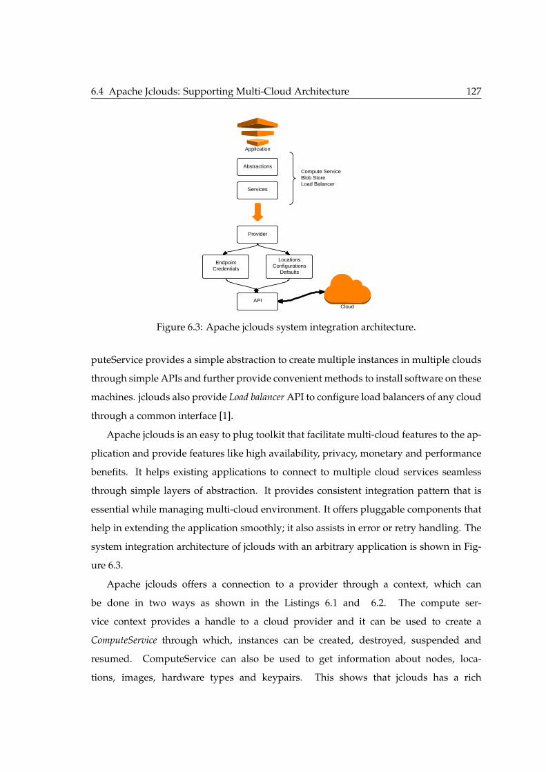
6.4 Apache Jclouds: Supporting Multi-Cloud Architecture 127
CloudAPI
Endpoint Credentials
Locations Configurations
Defaults
Services
AbstractionsCompute ServiceBlob StoreLoad Balancer
Provider
Application
Figure 6.3: Apache jclouds system integration architecture.
puteService provides a simple abstraction to create multiple instances in multiple clouds
through simple APIs and further provide convenient methods to install software on these
machines. jclouds also provide Load balancer API to configure load balancers of any cloud
through a common interface [1].
Apache jclouds is an easy to plug toolkit that facilitate multi-cloud features to the ap-
plication and provide features like high availability, privacy, monetary and performance
benefits. It helps existing applications to connect to multiple cloud services seamless
through simple layers of abstraction. It provides consistent integration pattern that is
essential while managing multi-cloud environment. It offers pluggable components that
help in extending the application smoothly; it also assists in error or retry handling. The
system integration architecture of jclouds with an arbitrary application is shown in Fig-
ure 6.3.
Apache jclouds offers a connection to a provider through a context, which can
be done in two ways as shown in the Listings 6.1 and 6.2. The compute ser-
vice context provides a handle to a cloud provider and it can be used to create a
ComputeService through which, instances can be created, destroyed, suspended and
resumed. ComputeService can also be used to get information about nodes, loca-
tions, images, hardware types and keypairs. This shows that jclouds has a rich
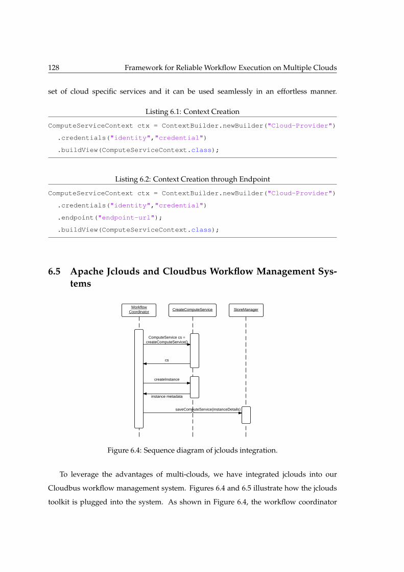
128 Framework for Reliable Workflow Execution on Multiple Clouds
set of cloud specific services and it can be used seamlessly in an effortless manner.
Listing 6.1: Context Creation
ComputeServiceContext ctx = ContextBuilder.newBuilder("Cloud-Provider")
.credentials("identity","credential")
.buildView(ComputeServiceContext.class);
Listing 6.2: Context Creation through Endpoint
ComputeServiceContext ctx = ContextBuilder.newBuilder("Cloud-Provider")
.credentials("identity","credential")
.endpoint("endpoint-url");
.buildView(ComputeServiceContext.class);
6.5 Apache Jclouds and Cloudbus Workflow Management Sys-tems
Workflow Coordinator CreateComputeService StoreManager
cs
createInstance
ComputeService cs = createComputeService()
instance metadata
saveComputeService(instanceDetails)
Figure 6.4: Sequence diagram of jclouds integration.
To leverage the advantages of multi-clouds, we have integrated jclouds into our
Cloudbus workflow management system. Figures 6.4 and 6.5 illustrate how the jclouds
toolkit is plugged into the system. As shown in Figure 6.4, the workflow coordinator
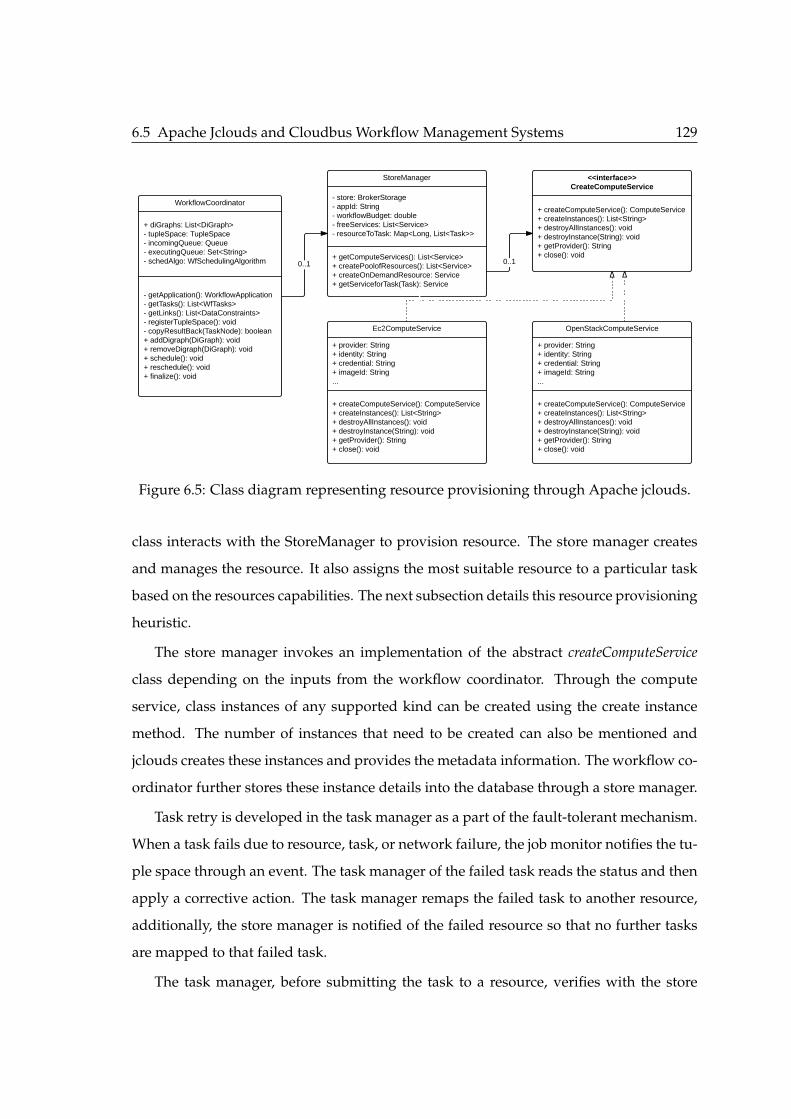
6.5 Apache Jclouds and Cloudbus Workflow Management Systems 129
WorkflowCoordinator
+ diGraphs: List<DiGraph>- tupleSpace: TupleSpace- incomingQueue: Queue- executingQueue: Set<String>- schedAlgo: WfSchedulingAlgorithm
- getApplication(): WorkflowApplication- getTasks(): List<WfTasks>- getLinks(): List<DataConstraints>- registerTupleSpace(): void- copyResultBack(TaskNode): boolean+ addDigraph(DiGraph): void+ removeDigraph(DiGraph): void+ schedule(): void+ reschedule(): void+ finalize(): void
StoreManager
- store: BrokerStorage- appId: String- workflowBudget: double- freeServices: List<Service>- resourceToTask: Map<Long, List<Task>>
+ getComputeServices(): List<Service>+ createPoolofResources(): List<Service>+ createOnDemandResource: Service+ getServiceforTask(Task): Service
<<interface>>CreateComputeService
+ createComputeService(): ComputeService+ createInstances(): List<String>+ destroyAllInstances(): void+ destroyInstance(String): void+ getProvider(): String+ close(): void
Ec2ComputeService
+ provider: String+ identity: String+ credential: String+ imageId: String...
+ createComputeService(): ComputeService+ createInstances(): List<String>+ destroyAllInstances(): void+ destroyInstance(String): void+ getProvider(): String+ close(): void
OpenStackComputeService
+ provider: String+ identity: String+ credential: String+ imageId: String...
+ createComputeService(): ComputeService+ createInstances(): List<String>+ destroyAllInstances(): void+ destroyInstance(String): void+ getProvider(): String+ close(): void
0..1 0..1
Figure 6.5: Class diagram representing resource provisioning through Apache jclouds.
class interacts with the StoreManager to provision resource. The store manager creates
and manages the resource. It also assigns the most suitable resource to a particular task
based on the resources capabilities. The next subsection details this resource provisioning
heuristic.
The store manager invokes an implementation of the abstract createComputeService
class depending on the inputs from the workflow coordinator. Through the compute
service, class instances of any supported kind can be created using the create instance
method. The number of instances that need to be created can also be mentioned and
jclouds creates these instances and provides the metadata information. The workflow co-
ordinator further stores these instance details into the database through a store manager.
Task retry is developed in the task manager as a part of the fault-tolerant mechanism.
When a task fails due to resource, task, or network failure, the job monitor notifies the tu-
ple space through an event. The task manager of the failed task reads the status and then
apply a corrective action. The task manager remaps the failed task to another resource,
additionally, the store manager is notified of the failed resource so that no further tasks
are mapped to that failed task.
The task manager, before submitting the task to a resource, verifies with the store
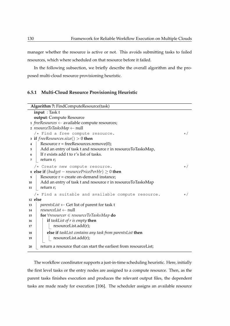
130 Framework for Reliable Workflow Execution on Multiple Clouds
manager whether the resource is active or not. This avoids submitting tasks to failed
resources, which where scheduled on that resource before it failed.
In the following subsection, we briefly describe the overall algorithm and the pro-
posed multi-cloud resource provisioning heuristic.
6.5.1 Multi-Cloud Resource Provisioning Heuristic
Algorithm 7: FindComputeResource(task)input : Task toutput: Compute Resource
1 freeResources← available compute resources;2 resourceToTasksMap← null/* Find a free compute resource. */
3 if f reeResources.size() > 0 then4 Resource r = freeResources.remove(0);5 Add an entry of task t and resource r in resourceToTasksMap,6 If r exists add t to r’s list of tasks.7 return r;
/* Create new compute resource. */8 else if (budget− resourcePricePerHr) ≥ 0 then9 Resource r = create on-demand instance;
10 Add an entry of task t and resource r in resourceToTasksMap11 return r;
/* Find a suitable and available compute resource. */12 else13 parentsList← Get list of parent for task t14 resourceList← null15 for ∀resourcer ∈ resourceToTasksMap do16 if taskList of r is empty then17 resourceList.add(r);
18 else if taskList contains any task from parentsList then19 resourceList.add(r);
20 return a resource that can start the earliest from resourceList;
The workflow coordinator supports a just-in-time scheduling heuristic. Here, initially
the first level tasks or the entry nodes are assigned to a compute resource. Then, as the
parent tasks finishes execution and produces the relevant output files, the dependent
tasks are made ready for execution [106]. The scheduler assigns an available resource
6.5 Apache Jclouds and Cloudbus Workflow Management Systems 131
to these ready tasks through a resource provisioning policy. The workflow coordinator
invokes this resource allocation to get a compute resource for the task.
The contribution of this chapter is developing a novel multi-cloud resource provision-
ing policy that allocates resources from two cloud providers and two types of resources
i.e., spot instances and on-demand instances.
The scheduling heuristic is also fault-tolerant. When a failure occurs, the task man-
ager is notified and it reschedules the failed task onto another resource and removes the
resource from the resource pool. This ensures that other tasks are not mapped to the
failed resource.
The proposed multi-cloud resource allocation policy is outlined in Algorithm 7. Ini-
tially, a pool of spot instances are created and assigned to the freeResources set. This is
done because spot instances take longer time to boot up [94]. The budget is given by the
user and the number of on-demand and spot resources created is based on this budget.
If the spot-instances go out-of-bid or extend beyond their charging period, the budget is
updated accordingly.
The proposed resource allocation policy initially finds a free resource for the given
task. On finding a free resource, the resourceToTasksMap is updated for book keeping. If
multiple free resources are found, the first resource is chosen. If no free resource is found
and if there is sufficient budget to create a new on-demand resource, then an on-demand
resource is instantiated. If there is no sufficient budget to create new instances, then the
resource allocation policy finds the best possible resource from the available resources.
The resource allocation policy evaluates all the resources and chooses a resource that is
available in the earliest. If possible, it selects a resource that is running a parent task as
it reduces the data transfer time. For this reason, the resource allocation policy creates a
list of all parents of the given task. It iterates through each resource from the resourceTo-
TasksMap adding suitable resources into a resourceList. It is a list of all feasible resources. If
the resource has no tasks then it is a free resource with no tasks running or scheduled on
it, therefore, the resource is added to the resource list. If the resource has tasks, i.e., run-
ning or scheduled tasks, then the policy checks whether the running or scheduled tasks
contain any of the parents tasks. If it does, then that resource will reduce the data transfer
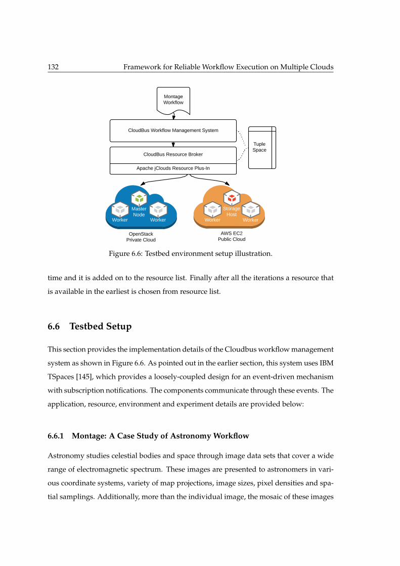
132 Framework for Reliable Workflow Execution on Multiple Clouds
Montage Workflow
OpenStackPrivate Cloud
AWS EC2Public Cloud
CloudBus Resource Broker
Apache jClouds Resource Plus-In
Storage Host
Master Node
WorkerWorker WorkerWorker
CloudBus Workflow Management System
Tuple Space
Figure 6.6: Testbed environment setup illustration.
time and it is added on to the resource list. Finally after all the iterations a resource that
is available in the earliest is chosen from resource list.
6.6 Testbed Setup
This section provides the implementation details of the Cloudbus workflow management
system as shown in Figure 6.6. As pointed out in the earlier section, this system uses IBM
TSpaces [145], which provides a loosely-coupled design for an event-driven mechanism
with subscription notifications. The components communicate through these events. The
application, resource, environment and experiment details are provided below:
6.6.1 Montage: A Case Study of Astronomy Workflow
Astronomy studies celestial bodies and space through image data sets that cover a wide
range of electromagnetic spectrum. These images are presented to astronomers in vari-
ous coordinate systems, variety of map projections, image sizes, pixel densities and spa-
tial samplings. Additionally, more than the individual image, the mosaic of these images
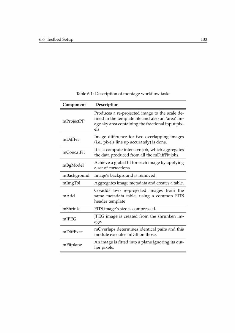
6.6 Testbed Setup 133
Table 6.1: Description of montage workflow tasks
Component Description
mProjectPP
Produces a re-projected image to the scale de-fined in the template file and also an ‘area’ im-age sky area containing the fractional input pix-els
mDiffFitImage difference for two overlapping images(i.e., pixels line up accurately) is done.
mConcatFitIt is a compute intensive job, which aggregatesthe data produced from all the mDiffFit jobs.
mBgModelAchieve a global fit for each image by applyinga set of corrections.
mBackground Image’s background is removed.
mImgTbl Aggregates image metadata and creates a table.
mAddCo-adds two re-projected images from thesame metadata table, using a common FITSheader template
mShrink FITS image’s size is compressed.
mJPEGJPEG image is created from the shrunken im-age.
mDiffExecmOverlaps determines identical pairs and thismodule executes mDiff on those.
mFitplaneAn image is fitted into a plane ignoring its out-lier pixels.

134 Framework for Reliable Workflow Execution on Multiple Clouds
Figure 6.7: Montage workflow.
holds greater importance and significance to astronomers representing significant struc-
tures, such as star formations, regions, and cluster of galaxies, etc.
These complexities require comprehensive image mosaic software that meets as-
tronomer’s requirements (e.g., coordinates, rotation, size, projections). The Montage
software toolkit is designed for this specific requirement. Montage widens astronomical
research avenues by enabling mosaic generation through software tools, and it also in-
cludes deep source detection by studying wavelength-dependent structures, combining
multiple wavelength data, and detecting minuscule features through image differencing.
Montage toolkit was designed to process tasks that compute such mosaics through
independent modules using simple executables. This toolkit can be run on desktops,
clusters, grids, supercomputers and clouds, and it effectively uses parallel computing
environments to scale and speed-up on as many processors as possible.
Montage application [16] is a complex astronomy workflow. We have used a montage
workflow consisting of 110 tasks, where the number of the tasks indicates the number of
images used. It is a I/O intensive application, which produces a mosaic of astronomic
images.
The Architecture of Montage
Montage computes an image mosaic through the following steps:
6.6 Testbed Setup 135
1 Re-projecting images onto a common coordinate system, spatial scale, and world
coordinate system projection.
2 Minimizing the inter-image differences and achieving common flux scales through
modeling the background radiation.
3 Rectifying background level and common flux scale of images.
4 Addition of re-projected and corrected images into a final mosaic.
The independent modules of the Montage toolkit that comprise of a workflow are
listed with brief description in Table 6.1 and the workflow of montage is depicted in
Figure 6.7.
6.6.2 Resource Characteristics
Workflow management system requires three kinds of resources:
• Master Node: this is where the portal, engine and the resource broker is hosted.
This node was hosted in the OpenStack private cloud.
• Storage Host: this node hosts all the data, input, output, and the intermediate files.
The node was in the Amazon AWS Sydney region.
• Worker Node: this node performs the workflow execution. It could be created
either in the OpenStack cloud or the Amazon AWS cloud.
Resources communicate with each other through password-less SSH. The configurations
for this where made in the cloud resources respectively.
6.6.3 Environment
We have used two cloud environments. We have used an OpenStack private cloud de-
ployed in The University of Melbourne. The OpenStack environment is setup on three
IBM X3500 M4 servers, each with 12 cores (2 x Intel Xeon 2.0GHz Processor , 15MB Cache)

136 Framework for Reliable Workflow Execution on Multiple Clouds
with 2.1 TB disk space and 64GB RAM. Instance of m1.tiny where used for worker nodes.
M2.4xlarge was used for the master node.
The second cloud we have considered is the Amazon EC2 cloud. We have considered
the Asia Pacific (Sydney) region as it is the closest to us and will have the minimum
latency. T1.Micro instances where used for worker and storage nodes in the public cloud.
6.6.4 Failure Model
Resource failures was orchestrated to demonstrate the fault-tolerance of the workflow
management system. mProjectPP and mBackground tasks types where choosen to be
failed, as they are higher in number and they affect two levels of workflow execution.
The workflow variant we have choosen has 25 tasks each of these types. Failing any of
these task impacts the execution similarly. Three from each of these types where choosen
randomly. A combination of these two types among the randomly choosen tasks where
failed based on the failure size given as an input. For example if a failure size of 3 was
given as an input, one task of type mProjectPP and two mBackground where selected
and their corresponding resources where terminated to orchestrate failure events.
6.7 Results
In this section, the results to illustrate the key contributions of this chapter are provided.
The resource provisioner instantiated a pool of spot instances initially on the public AWS
cloud and on-demand instances where created when needed on private cloud. The fault-
tolerance and on-demand provisioning of our system are discussed in this section.
Figure 6.8 illustrates the effect of failures on the workflow makespan. We can observe
that as the failures increase, the makespan increases. Since a retry fault-tolerant technique
is used, failures increase the makespan. This experiment demonstrates that the workflow
management system can mitigate resource or other failures and can successfully retry the
task on another resource ensuring successful execution. After a resource fails, the algo-
rithm remaps all tasks that where scheduled on the failed resource, thus saving execution
time.
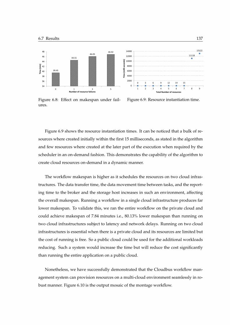
6.7 Results 137
39.45
44.55
46.05
46.92
34
36
38
40
42
44
46
48
0 1 3 5
Tim
e (
min
)
Number of resource failures
Figure 6.8: Effect on makespan under fail-ures.
0 3 6 9 12 14 15
11118
13122
0
2000
4000
6000
8000
10000
12000
14000
1 2 3 4 5 6 7 8 9
Tim
e (
mil
li s
eco
nd
s)
Total Number of resources
Figure 6.9: Resource instantiation time.
Figure 6.9 shows the resource instantiation times. It can be noticed that a bulk of re-
sources where created initially within the first 15 milliseconds, as stated in the algorithm
and few resources where created at the later part of the execution when required by the
scheduler in an on-demand fashion. This demonstrates the capability of the algorithm to
create cloud resources on-demand in a dynamic manner.
The workflow makespan is higher as it schedules the resources on two cloud infras-
tructures. The data transfer time, the data movement time between tasks, and the report-
ing time to the broker and the storage host increases in such an environment, affecting
the overall makespan. Running a workflow in a single cloud infrastructure produces far
lower makespan. To validate this, we ran the entire workflow on the private cloud and
could achieve makespan of 7.84 minutes i.e., 80.13% lower makespan than running on
two cloud infrastructures subject to latency and network delays. Running on two cloud
infrastructures is essential when there is a private cloud and its resources are limited but
the cost of running is free. So a public cloud could be used for the additional workloads
reducing. Such a system would increase the time but will reduce the cost significantly
than running the entire application on a public cloud.
Nonetheless, we have successfully demonstrated that the Cloudbus workflow man-
agement system can provision resources on a multi-cloud environment seamlessly in ro-
bust manner. Figure 6.10 is the output mosaic of the montage workflow.
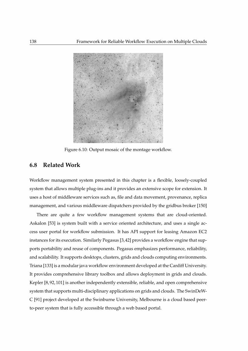
138 Framework for Reliable Workflow Execution on Multiple Clouds
Figure 6.10: Output mosaic of the montage workflow.
6.8 Related Work
Workflow management system presented in this chapter is a flexible, loosely-coupled
system that allows multiple plug-ins and it provides an extensive scope for extension. It
uses a host of middleware services such as, file and data movement, provenance, replica
management, and various middleware dispatchers provided by the gridbus broker [150]
There are quite a few workflow management systems that are cloud-oriented.
Askalon [53] is system built with a service oriented architecture, and uses a single ac-
cess user portal for workflow submission. It has API support for leasing Amazon EC2
instances for its execution. Similarly Pegasus [3,42] provides a workflow engine that sup-
ports portability and reuse of components. Pegasus emphasizes performance, reliability,
and scalability. It supports desktops, clusters, grids and clouds computing environments.
Triana [133] is a modular java workflow environment developed at the Cardiff University.
It provides comprehensive library toolbox and allows deployment in grids and clouds.
Kepler [8,92,101] is another independently extensible, reliable, and open comprehensive
system that supports multi-disciplinary applications on grids and clouds. The SwinDeW-
C [91] project developed at the Swinburne University, Melbourne is a cloud based peer-
to-peer system that is fully accessible through a web based portal.

6.9 Summary 139
In comparison to the above listed projects, our workflow management system renders
a decentralized scheduling architecture and also allows a loosely-coupled architecture
that fosters modularity and aids extensibility. Additionally, this workflow management
system has introduced a multi-cloud feature that will facilitate the execution of workflow
tasks on multiple cloud infrastructures.
6.9 Summary
In this chapter, the Cloudbus workflow management system a project of CLOUDS Lab
at the University of Melbourne has been extended to support dynamic provisioning of
cloud resources, supporting multiple cloud providers. This extension to support mul-
tiple cloud providers is achieved through the integration of opensource Apache jclouds
toolkit. We have also presented a resource provisioning algorithm for a multi-cloud en-
vironment. Additionally, we have implemented a retry fault-tolerant mechanism to mit-
igate failures at task, resource or network levels. Faults at various task stages, such as
ready, submitted, stage-in, stage-out can be handled seamlessly and this is demonstrated
through our experiments using an astronomy application case study.

This page intentionally left blank.
Chapter 7
Conclusions and Future Directions
This chapter summarizes the research work on robust and fault-tolerant workflow scheduling on
cloud computing platforms presented in this thesis and highlights the major findings. It also
outlines the future directions and open research challenges in this area.
7.1 Summary of Contributions
CLOUD computing offers low-cost computing services as a subscription based ser-
vice, which are elastically scalable, and dynamically provisioned. Additionally, it
also provides attractive pricing models like on-demand and spot instances. Because of
which, scientific workflow management systems are rapidly moving towards it. How-
ever, cloud environments are prone to failures and performance variations among re-
sources.
In this regard, this thesis set out with one core objective to develop fault-tolerant
scheduling algorithms for workflows. To accomplish this, we proposed and investigated
various fault-tolerant techniques, pricing models, scheduling heuristics, and resource se-
lection policies. Further, in this section we detail each of these findings.
Fault-tolerance is crucial for such large scale complex applications running on failure-
prone distributed environments. Given the large body of research in this area, in chap-
ter 2, we provided a comprehensive view on fault-tolerance for workflows in various
distributed environments.
In particular, this chapter provided a detailed understanding of faults from a generic
viewpoint (e.g. transient, intermittent, and permanent) and a processor viewpoint (such
141

142 Conclusions and Future Directions
as, crash, fail-stop and byzantine). It also described techniques such as replication re-
submission, checkpointing, provenance, rescue-workflow, exception handling, alternate
task, failure masking, slack time, and trust-based approaches used to resolve these faults
by which, a transparent and seamless experience to workflow users can be offered.
Apart from the fault-tolerant techniques, we provided an insight into numerous fail-
ure models and metrics. Metrics range from makespan oriented, probabilistic based, re-
liability based, and trust-based among others. These metrics inform us about the quality
of the schedule and quantify fault-tolerance of a schedule.
Prominent WFMSs are detailed and positioned with respect to their features, charac-
teristics, and uniqueness. Lastly, tools such as those for describing workflow languages,
data-management, security and fault-tolerance, tools that aid in cloud development, and
support systems (including social networking environments, and workflow generators),
were introduced.
Chapter 3 presented three resource allocation policies with robustness, makespan,
and cost as its objectives. This is one of the early works in robust and fault-tolerant work-
flow scheduling on Clouds, considering deadline and budget constraints. The resource
allocation policies judiciously add slack time to make the schedule robust considering
the deadline and budget constraints. We test our policies with two failure models for five
scientific workflows with two metrics for robustness. Results indicated that our policies
are robust against uncertainties like task failures and performance variations of VMs.
Among the proposed policies presented, one of the policies showed the highest ro-
bustness and at the same time minimized makespan of the workflow. This policy pro-
vided a robust schedule with costs marginally higher than the reference algorithms con-
sidered. The weights of the weighted policy presented in this chapter can be varied
according to the user priorities. Overall, our policies provided robust schedules with a
the lowest possible makespan. They also show that with increase in budget, our policies
increase the robustness of the schedule with reasonable increase in cost.
In Chapter 4, two scheduling heuristics that map workflow tasks onto spot and on-
demand instance were presented. They minimize the execution cost by intelligently uti-
lizing the variety of pricing models offered by the cloud providers. They are shown to
7.2 Future Research Directions 143
be robust and fault-tolerant towards out-of-bid failures and performance variations of
cloud instances. A bidding strategy that bids in accordance to the workflow require-
ments to minimize the cost was also presented. This work also demonstrated the use of
checkpointing and offers cost savings up to 14%. Simulation results showed that cost re-
ductions of upto 70% were achieved under relaxed deadlines, when spot instances were
used.
In Chapter 5, we have proposed two just-in-time adaptive workflow scheduling
heuristics for clouds that use task retry and task replication fault-tolerant techniques.
These heuristics use on-demand and spot instances to provide fault-tolerant schedules
whilst minimizing time and cost. They are fault-tolerant against performance variations,
out-of-bid failures, and resource failures. Extensive simulations have shown that the pro-
posed heuristics generate schedules with significantly lower failure probabilities. The
makespan of these schedules are also much lower than the baseline algorithm. These
heuristics are also shown to maximize resource utilization. These experiments establish
that pricing models offered by cloud providers can be used to reduce costs and makespan
and at the same time offer robust and resilient schedules.
Finally, in Chapter 6 we have developed a multi-cloud framework for the cloudbus
workflow management system. Workflow applications can use this resource plug-in
to schedule resources in a multi-cloud environment. We demonstrated this capability
through an astronomy workflow application case study using a openstack private cloud
and an Amazon AWS public cloud. In this chapter we also developed a novel heuristic
for multi-cloud environment.
7.2 Future Research Directions
The research pertaining to thesis is expected to continuously evolve along with the devel-
opments in the cloud computing field. Therefore, the challenges and issues also evolve
and need fresh contributions. In spite of the significant contributions of this thesis in de-
veloping fault-tolerant scheduling algorithms for cloud computing platforms, there are
several open research challenges that need to be addressed. This section delineates open
144 Conclusions and Future Directions
research areas and future directions in this regard.
7.2.1 Cloud Failure Characteristics
Although fault types are known in the current works, the frequency of each type of fail-
ure, especially in a cloud environment, is not publicly available. There are few traces of
public cloud failures; however, the information that can be obtained from them is min-
imal. Understanding failures and their frequencies in cloud environments can enhance
the research of robust workflow management. Failure rates and types vary among pri-
vate clouds, public clouds, multi-cloud, hybrid clouds, and commodity clouds. Similarly,
understanding performance variations of resources among various types of clouds is an
open area of research with a great importance to develop robust and reliable WFMSs
tailored for each of these environments.
7.2.2 Metrics for Fault-Tolerance
Quantifying fault-tolerance is another challenge as there are multiple metrics with no
proper consensus among them. Metrics have been developed for specific problems for
various computing environments with multiple assumptions. Developing a generic met-
ric applicable for multiple mechanisms and environments can help to compare different
fault-tolerant mechanisms and rank them based on their performance. Proposing such
a widely acceptable metric would be a significant contribution in this domain. In this
thesis, prominent metrics have been documented that can be helpful in this research.
7.2.3 Cloud Pricing Models
Pricing is an important aspect for a cloud environment. Research that consider a com-
bination of pricing models and their SLAs to provide fault-tolerant mechanisms that are
cost-effective are still in their infancy. Additionally, analyzing the impact of the fault-
tolerant mechanisms on the incurred cost is also essential. For example, replication uses
more resources and adds more cost to the schedule; on the other hand, resubmission in-
creases the execution time with slight increase in cost. It is important to understand the
7.2 Future Research Directions 145
cost implications of a particular fault-tolerant mechanism.
Recently, spot instance characteristics have also changed. Amazon allows a two
minute notice before terminating the instances. This allows for better fault-tolerant be-
havior. Our proposed algorithms can be extended to addresses this development and
this can provided further fault-tolerance in a schedule.
Different cloud providers price instances with different time units. Some price in-
stances per hour, some per minute with or without a flag fall. These pricing behaviors
impact different workflows in multiple ways. Choosing the right pricing model for spe-
cific workflows is an exciting research question. Added to this, investigation into fault-
tolerance in such environments is challenging and needs to be addressed.
7.2.4 Multiple Tasks on a Single Instance
Traditionally, workflows schedule one task on one instance at a given time. However,
cloud resources are multi-core processors and some workflow tasks are not moldable
i.e., they are not multi-threaded and cannot use all the processors. Therefore, scheduling
multiple tasks on a single instance can enable significant cost benefits, although the per-
formance might be impacted. Additionally, it increases the failure probability of those
tasks. This is open area where new heuristics can be developed for such a combination
of challenges.
7.2.5 Workflow Specific Scheduling
WFMSs can typically run a single workflow, multiple workflows, or a workflow ensem-
ble, i.e., it might vary from a single workflow to a collection of workflows of similar
or different types. Challenges in each context are unique and the allocation mechanism
must consider this perspective. Associating this aspect with fault-tolerance will make
WFMSs more resilient.
A deep understanding of the workflow helps in developing efficient algorithms.
Data-intensive workflows require different allocation and fault-tolerant mechanisms
than a compute-intensive workflow. WFMS or the user should be able to identify the
146 Conclusions and Future Directions
workflow types and address their constraints. Intelligent systems need to be built that
can capture this information and devise schedule in lieu with them.
7.2.6 Multi-Cloud Challenges
Workflow scheduling, specially for e-science application, involves collaborations spread
across geographic regions. Using a multi-cloud environment could address the latency
issues involved. However, the prices of resources change from region to region. The
failure rates of resources are different. The data transfer cost would need to considered.
Models need to be developed to schedule on such a system with multiple heterogeneity.
The study of cost and time implications would be a significant contribution in this area.
7.2.7 Energy-Efficient Scheduling
Cloud infrastructures consume vast amount of energy leaving large carbon footprints.
Added to this, increase in electricity prices stress the need for energy efficient data cen-
ters. Therefore cloud providers and applications using cloud infrastructures must de-
velop energy efficient solutions.
Workflow scheduling algorithms extensively use large number of cloud resources.
Hence, a focus on energy-efficient workflow scheduling is much required in addition to
existing performance parameters.
7.3 Final Remarks
Cloud computing offers virtualized servers, which are dynamically managed, monitored,
maintained, and governed by market principles. As a subscription based computing ser-
vice, it provides a convenient platform for scientific workflows due to features like appli-
cation scalability, heterogeneous resources, dynamic resource provisioning, and pay-as-
you-go cost model. Fault-tolerant scheduling heuristics developed in this thesis enable
workflow managements system to schedule complex large scale workflow applications
on cloud computing platforms in a robust and fault-tolerant manner whilst minimizing

7.3 Final Remarks 147
time and cost. Research such as this, is essential due to the performance variations ex-
perienced among cloud resources and various kinds of failure found in the application,
environment and the network. The contributions of this thesis helps in making the exe-
cution of workflow seamless on cloud computing platforms.

This page intentionally left blank.
Bibliography
[1] “Apache jclouds,” https://jclouds.apache.org/, 2014, [Online; accessed 12-May-
2015].
[2] “Pegasus workflow generator,” https://confluence.pegasus.isi.edu/display/
pegasus/WorkflowGenerator/, 2014, [Online; accessed 5-December-2014].
[3] “Pegasus workflow management system,” https://pegasus.isi.edu/, 2014, [On-
line; accessed 01-December-2014].
[4] S. Abrishami, M. Naghibzadeh, and D. Epema, “Cost-driven scheduling of grid
workflows using partial critical paths,” IEEE Transactions on Parallel and Distributed
Systems, vol. 23, no. 8, pp. 1400 –1414, aug. 2012.
[5] ——, “Deadline-constrained workflow scheduling algorithms for infrastructure as
a service clouds,” Future Generation Computer Systems, vol. 29, no. 1, pp. 158 – 169,
2013.
[6] S. Adabi, A. Movaghar, and A. M. Rahmani, “Bi-level fuzzy based advanced reser-
vation of cloud workflow applications on distributed grid resources,” The Journal
of Supercomputing, vol. 67, no. 1, pp. 175–218, 2014.
[7] O. Alacam and M. Dalcı, “A usability study of webmaps with eye tracking tool:
The effects of iconic representation of information,” in Proceedings of the 13th Inter-
national Conference on Human-Computer Interaction., Sep 2009, pp. 12–21.
[8] I. Altintas, C. Berkley, E. Jaeger, M. Jones, B. Ludascher, and S. Mock, “Kepler: an
extensible system for design and execution of scientific workflows,” in Proceedings
149
150 BIBLIOGRAPHY
of the 16th International Conference on Scientific and Statistical Database Management.,
June 2004, pp. 423–424.
[9] K. Amin, G. von Laszewski, M. Hategan, N. Zaluzec, S. Hampton, and A. Rossi,
“Gridant: a client-controllable grid workflow system,” in Proceedings of the 37th
Annual Hawaii International Conference on System Sciences., Jan 2004, pp. 10–pp.
[10] M. Armbrust, A. Fox, R. Griffith, A. Joseph, R. Katz, A. Konwinski, G. Lee, D. Pat-
terson, A. Rabkin, I. Stoica, and M. Zaharia, “A view of cloud computing,” ACM
Communications, vol. 53, no. 4, pp. 50–58, Apr. 2010.
[11] O. Ben-Yehuda, M. Ben-Yehuda, A. Schuster, and D. Tsafrir, “Deconstructing ama-
zon EC2 spot instance pricing,” in Proceedings of the IEEE 3rd International Conference
on Cloud Computing Technology and Science, 2011.
[12] A. Benoit, M. Hakem, and Y. Robert, “Fault tolerant scheduling of precedence task
graphs on heterogeneous platforms,” in Proceedings of the IEEE International Sympo-
sium on Parallel and Distributed Processing, 2008. IPDPS 2008., April 2008, pp. 1–8.
[13] A. Benoit, L.-C. Canon, E. Jeannot, and Y. Robert, “Reliability of task graph sched-
ules with transient and fail-stop failures: complexity and algorithms,” Journal of
Scheduling, vol. 15, no. 5, pp. 615–627, 2012.
[14] A. Benoit, M. Hakem, and Y. Robert, “Multi-criteria scheduling of precedence task
graphs on heterogeneous platforms,” The Computer Journal, vol. 53, no. 6, pp. 772–
785, 2010.
[15] F. Berman, H. Casanova, A. Chien, K. Cooper, H. Dail, A. Dasgupta, W. Deng,
J. Dongarra, L. Johnsson, K. Kennedy, C. Koelbel, B. Liu, X. Liu, A. Mandal,
G. Marin, M. Mazina, J. Mellor-Crummey, C. Mendes, A. Olugbile, M. Patel,
D. Reed, Z. Shi, O. Sievert, H. Xia, and A. YarKhan, “New grid scheduling and
rescheduling methods in the GrADS project,” International Journal of Parallel Pro-
gramming, vol. 33, no. 2-3, pp. 209–229, 2005.
BIBLIOGRAPHY 151
[16] G. Berriman, E. Deelman, J. Good, J. Jacob, D. Katz, A. Laity, T. Prince, G. Singh, and
M.-H. Su, “Generating complex astronomy workflows,” in Workflows for e-Science,
I. Taylor, E. Deelman, D. Gannon, and M. Shields, Eds., 2007, pp. 19–38.
[17] L. Boloni and D. C. Marinescu, “Robust scheduling of metaprograms,” Journal of
Scheduling, vol. 5, no. 5, pp. 395–412, 2002.
[18] I. Brandic, D. Music, and S. Dustdar, “Service mediation and negotiation bootstrap-
ping as first achievements towards self-adaptable grid and cloud services,” in Pro-
ceedings of the 6th International Conference Industry Session on Grids Meets Autonomic
Computing, ser. GMAC ’09, New York, NY, USA, 2009, pp. 1–8.
[19] R. Buyya, S. Pandey, and C. Vecchiola, “Cloudbus toolkit for market-oriented
cloud computing,” in Cloud Computing, ser. Lecture Notes in Computer Science,
M. Jaatun, G. Zhao, and C. Rong, Eds., 2009, vol. 5931, pp. 24–44.
[20] R. Calheiros and R. Buyya, “Meeting deadlines of scientific workflows in public
clouds with tasks replication,” IEEE Transactions on Parallel and Distributed Systems,,
vol. 25, no. 5, pp. 1787–1796, 2014.
[21] R. Calheiros, R. Ranjan, A. Beloglazov, C. De Rose, and R. Buyya, “CloudSim: a
toolkit for modeling and simulation of cloud computing environments and evalua-
tion of resource provisioning algorithms,” Software: Practice and Experience,, vol. 41,
no. 1, pp. 23–50, 2011.
[22] S. P. Callahan, J. Freire, E. Santos, C. E. Scheidegger, C. T. Silva, and H. T. Vo, “Vis-
trails: Visualization meets data management,” in Proceedings of the ACM SIGMOD
International Conference on Management of Data, ser. SIGMOD ’06, New York, NY,
USA, 2006, pp. 745–747.
[23] L. Canon and E. Jeannot, “Evaluation and optimization of the robustness of dag
schedules in heterogeneous environments,” IEEE Transactions on Parallel and Dis-
tributed Systems, vol. 21, no. 4, pp. 532–546, 2010.

152 BIBLIOGRAPHY
[24] J. Cao, S. A. Jarvis, S. Saini, and G. R. Nudd, “Gridflow: workflow management
for grid computing,” in Proceedings of the 3rd IEEE/ACM International Symposium on
Cluster Computing and the Grid. CCGrid., May 2003, pp. 198–205.
[25] J. Chen and Y. Yang, “Adaptive selection of necessary and sufficient checkpoints
for dynamic verification of temporal constraints in grid workflow systems,” ACM
Transactions on Autonomous and Adaptive Systems, vol. 2, no. 2, Jun. 2007.
[26] W. Chen and E. Deelman, “Fault tolerant clustering in scientific workflows,” in
Proceedings of the IEEE 8th World Congress on Services. SERVICES., June 2012, pp.
9–16.
[27] A. Chervenak, E. Deelman, M. Livny, M. Su, R. Schuler, S. Bharathi, G. Mehta, and
K. Vahi, “Data placement for scientific applications in distributed environments,”
in Proceedings of the 8th IEEE/ACM International Conference on Grid Computing, ser.
GRID ’07, Washington, DC, USA, 2007, pp. 267–274.
[28] A. Chervenak, E. Deelman, M. Livny, M. H. Su, R. Schuler, S. Bharathi, G. Mehta,
and K. Vahi, “Data placement for scientific applications in distributed environ-
ments,” in Proceedings of the 8th IEEE/ACM International Conference on Grid Com-
puting, ser. GRID ’07, Sep 2007, pp. 267–274.
[29] N. Chohan, C. Castillo, M. Spreitzer, M. Steinder, A. Tantawi, and C. Krintz, “See
spot run: using spot instances for mapreduce workflows,” in Proceedings of the 2nd
USENIX conference on Hot Topics in cloud Computing. USENIX Association, 2010.
[30] W. Cirne and F. Berman, “A model for moldable supercomputer jobs,” in Proceed-
ings of 15th International Symposium of Parallel and Distributed Processing., 2001, pp.
8–pp.
[31] W. Cirne, F. Brasileiro, D. Paranhos, L. Goes, and W. Voorsluys, “On the efficacy,
efficiency and emergent behavior of task replication in large distributed systems,”
Parallel Computing, vol. 33, no. 3, pp. 213 – 234, 2007.

BIBLIOGRAPHY 153
[32] C. Dabrowski, “Reliability in grid computing systems,” Concurrency and Computa-
tion: Practice and Experience, vol. 21, no. 8, pp. 927–959, 2009.
[33] S. Darbha and D. Agrawal, “A task duplication based optimal scheduling algo-
rithm for variable execution time tasks,” in Proceedings of the International Confer-
enceon Parallel Processing. Vol. 1. ICPP., vol. 2, Aug 1994, pp. 52–56.
[34] A. Dastjerdi and R. Buyya, “An autonomous reliability-aware negotiation strategy
for cloud computing environments,” in Proceedings of the 12th IEEE/ACM Interna-
tional Symposium on Cluster, Cloud and Grid Computing (CCGrid), 2012. IEEE, 2012,
pp. 284–291.
[35] S. B. Davidson, S. C. Boulakia, A. Eyal, B. Ludascher, T. M. McPhillips, S. Bowers,
M. K. Anand, and J. Freire, “Provenance in scientific workflow systems.” IEEE Data
Eng. Bull., vol. 30, no. 4, pp. 44–50, 2007.
[36] S. B. Davidson and J. Freire, “Provenance and scientific workflows: Challenges
and opportunities,” in Proceedings of the ACM SIGMOD International Conference on
Management of Data, ser. SIGMOD ’08, New York, NY, USA, 2008, pp. 1345–1350.
[37] J. Dean, “Experiences with mapreduce, an abstraction for large-scale computation,”
in Proceedings of the 15th International Conference on Parallel Architectures and Compi-
lation Techniques, ser. PACT ’06, 2006.
[38] ——, “Software engineering advice from building large-scale distributed systems,”
http://research.google.com/people/jeff/stanford-295-talk.pdf, 2007.
[39] J. Dean and S. Ghemawat, “MapReduce: Simplified data processing on large clus-
ters,” Communications of the ACM, vol. 51, no. 1, pp. 107–113, Jan 2008.
[40] E. Deelman, J. Blythe, Y. Gil, C. Kesselman, G. Mehta, S. Patil, M. H. Su, K. Vahi,
and M. Livny, “Pegasus: Mapping scientific workflows onto the grid,” in Grid Com-
puting, ser. Lecture Notes in Computer Science, M. Dikaiakos, Ed., 2004, vol. 3165,
pp. 11–20.
154 BIBLIOGRAPHY
[41] E. Deelman, D. Gannon, M. Shields, and I. Taylor, “Workflows and e-science: An
overview of workflow system features and capabilities,” Future Generation Com-
puter Systems, vol. 25, no. 5, pp. 528 – 540, 2009.
[42] E. Deelman, G. Singh, M. H. Su, J. Blythe, Y. Gil, C. Kesselman, G. Mehta, K. Vahi,
G. B. Berriman, J. Good, A. Laity, and K. D. S. Jacob, J. C., “Pegasus: A framework
for mapping complex scientific workflows onto distributed systems,” Scientific Pro-
gramming, vol. 13, no. 3, pp. 219–237, 2005.
[43] E. Deelman, K. Vahi, G. Juve, M. Rynge, S. Callaghan, P. J. Maechling, R. Mayani,
W. Chen, R. F. da Silva, M. Livny, and K. Wenger, “Pegasus, a workflow manage-
ment system for science automation,” Future Generation Computer Systems, vol. 46,
no. C, pp. 17 – 35, 2015.
[44] J. Dejun, G. Pierre, and C. Chi, “EC2 performance analysis for resource provision-
ing of service-oriented applications,” in Workshop on Service-Oriented Computing.
ICSOC/ServiceWave 2009. Springer, 2010, pp. 197–207.
[45] A. Dogan and F. Ozguner, “LDBS: a duplication based scheduling algorithm for
heterogeneous computing systems,” in Proceedings of the International Conference on
Parallel Processing., 2002, pp. 352–359.
[46] J. J. Dongarra, E. Jeannot, E. Saule, and Z. Shi, “Bi-objective scheduling algorithms
for optimizing makespan and reliability on heterogeneous systems,” in Proceedings
of the 19th Annual ACM Symposium on Parallel Algorithms and Architectures, ser. SPAA
’07, New York, NY, USA, 2007, pp. 280–288.
[47] A. B. Downey, A model for speedup of parallel programs, 1997.
[48] R. Duan, R. Prodan, and T. Fahringer, “DEE: a distributed fault tolerant workflow
enactment engine for grid computing,” in High Performance Computing and Commu-
nications, ser. Lecture Notes in Computer Science, L. Yang, O. Rana, B. Di Martino,
and J. Dongarra, Eds., 2005, vol. 3726, pp. 704–716.
BIBLIOGRAPHY 155
[49] I. Egwutuoha, D. Levy, B. Selic, and S. Chen, “A survey of fault tolerance mech-
anisms and checkpoint/restart implementations for high performance computing
systems,” The Journal of Supercomputing, vol. 65, no. 3, pp. 1302–1326, 2013.
[50] E. Elmroth, F. Hernandez, and J. Tordsson, “A light-weight grid workflow execu-
tion engine enabling client and middleware independence,” in Parallel Processing
and Applied Mathematics, ser. Lecture Notes in Computer Science, R. Wyrzykowski,
J. Dongarra, K. Karczewski, and J. Wasniewski, Eds., 2008, vol. 4967, pp. 754–761.
[51] E. N. Elnozahy, L. Alvisi, Y. Wang, and D. B. Johnson, “A survey of rollback-
recovery protocols in message-passing systems,” ACM Computing Surveys, vol. 34,
no. 3, pp. 375–408, Sep. 2002.
[52] T. Fahringer, A. Jugravu, S. Pllana, R. Prodan, C. Seragiotto, and H. Truong,
“Askalon: a tool set for cluster and grid computing,” Concurrency and Computation:
Practice and Experience, vol. 17, no. 2-4, pp. 143–169, 2005.
[53] T. Fahringer, R. Prodan, R. Duan, J. Hofer, F. Nadeem, F. Nerieri, S. Podlipnig,
J. Qin, M. Siddiqui, H. Truong, A. Villazon, and M. Wieczorek, “Askalon: A devel-
opment and grid computing environment for scientific workflows,” in Workflows
for e-Science, I. Taylor, E. Deelman, D. Gannon, and M. Shields, Eds., 2007, pp. 450–
471.
[54] T. Fahringer, R. Prodan, R. Duan, F. Nerieri, S. Podlipnig, J. Qin, M. Siddiqui,
H. Truong, A. Villazon, and M. Wieczorek, “Askalon: A grid application devel-
opment and computing environment,” in Proceedings of the 6th IEEE/ACM Interna-
tional Workshop on Grid Computing, ser. GRID ’05, Washington, DC, USA, 2005, pp.
122–131.
[55] C. Fayad, J. Garibaldi, and D. Ouelhadj, “Fuzzy grid scheduling using tabu search,”
in Proceedings of the IEEE International Conference on Fuzzy Systems. FUZZ-IEEE 2007,
July 2007, pp. 1 –6.
[56] I. Foster, J. Vockler, M. Wilde, and Y. Zhao, “Chimera: a virtual data system for
representing, querying, and automating data derivation,” in Proceedings of the 14th
156 BIBLIOGRAPHY
International Conference on Scientific and Statistical Database Management., 2002, pp.
37–46.
[57] Y. Gao, S. Gupta, Y. Wang, and M. Pedram, “An energy-aware fault tolerant
scheduling framework for soft error resilient cloud computing systems,” in Pro-
ceedings of the Design, Automation and Test in Europe Conference and Exhibition (DATE),
2014, March 2014, pp. 1–6.
[58] S. K. Garg, S. Versteeg, and R. Buyya, “A framework for ranking of cloud comput-
ing services,” Future Generation Computer Systems, vol. 29, no. 4, pp. 1012 – 1023,
2013, special Section: Utility and Cloud Computing.
[59] F. Gartner, “Fundamentals of fault-tolerant distributed computing in asynchronous
environments,” ACM Computing Surveys, vol. 31, no. 1, pp. 1–26, Mar. 1999.
[60] S. Ghemawat, H. Gobioff, and S. Leung, “The google file system,” in Proceedings of
the 19th ACM Symposium on Operating Systems Principles, ser. SOSP ’03, Oct 2003,
pp. 29–43.
[61] Y. Gil, E. Deelman, M. Ellisman, T. Fahringer, G. Fox, D. Gannon, C. Goble,
M. Livny, L. Moreau, and J. Myers, “Examining the challenges of scientific work-
flows,” Computer, vol. 40, no. 12, pp. 24–32, 2007.
[62] C. A. Goble and D. C. De Roure, “myExperiment: Social networking for workflow-
using e-scientists,” in Proceedings of the 2nd Workshop on Workflows in Support of
Large-scale Science, ser. WORKS ’07, New York, NY, USA, 2007, pp. 1–2.
[63] N. Grozev and R. Buyya, “Multi-cloud provisioning and load distribution for three-
tier applications,” ACM Transactions on Autonomous and Adaptive Systems, vol. 9,
no. 3, pp. 13:1–13:21, Oct. 2014.
[64] K. Hashimoto, T. Tsuchiya, and T. Kikuno, “Effective scheduling of duplicated
tasks for fault tolerance in multiprocessor systems,” IEICE Transactions on Infor-
mation and Systems, vol. 85, no. 3, pp. 525–534, 2002.
BIBLIOGRAPHY 157
[65] W. Herroelen and R. Leus, “Project scheduling under uncertainty: Survey and re-
search potentials,” European journal of operational research, vol. 165, no. 2, pp. 289–
306, 2005.
[66] H. Hiden, S. Woodman, P. Watson, and J. Cala, “Developing cloud applications
using the e-science central platform,” Philosophical Transactions of the Royal Society of
London A: Mathematical, Physical and Engineering Sciences, vol. 371, no. 1983, 2012.
[67] S. Hwang and C. Kesselman, “Grid workflow: a flexible failure handling frame-
work for the grid,” in Proceedings of the 12th IEEE International Symposium on High
Performance Distributed Computing., June 2003, pp. 126–137.
[68] A. Iosup, M. Jan, O. Sonmez, and D. Epema, “On the dynamic resource availability
in grids,” in Proceedings of the 8th IEEE/ACM International Conference on Grid Com-
puting, ser. GRID ’07, Washington, DC, USA, 2007, pp. 26–33.
[69] M. Isard, M. Budiu, Y. Yu, A. Birrell, and D. Fetterly, “Dryad: Distributed data-
parallel programs from sequential building blocks,” in Proceedings of the 2nd ACM
SIGOPS/EuroSys European Conference on Computer Systems, ser. EuroSys ’07, 2007,
pp. 59–72.
[70] B. Javadi, J. Abawajy, and R. Buyya, “Failure-aware resource provisioning for hy-
brid cloud infrastructure,” Journal of Parallel and Distributed Computing, vol. 72,
no. 10, pp. 1318 – 1331, 2012.
[71] B. Javadi, R. Thulasiram, and R. Buyya, “Statistical modeling of spot instance prices
in public cloud environments,” in Proceedings of the 4th IEEE International Conference
on Utility and Cloud Computing, 2011, pp. 219–228.
[72] B. Javadi, D. Kondo, A. Iosup, and D. Epema, “The failure trace archive: Enabling
the comparison of failure measurements and models of distributed systems,” Jour-
nal of Parallel and Distributed Computing, vol. 73, no. 8, pp. 1208 – 1223, 2013.
[73] D. Johnson and M. Garey, Computers and Intractability-A Guide to the Theory of NP-
Completeness, 1979.
158 BIBLIOGRAPHY
[74] G. Juve, A. Chervenak, E. Deelman, S. Bharathi, G. Mehta, and K. Vahi, “Char-
acterizing and profiling scientific workflows,” Future Generation Computer Systems,
vol. 29, no. 3, 2013.
[75] G. Juve and E. Deelman, “Scientific workflows and clouds,” Crossroads, vol. 16,
no. 3, pp. 14–18, 2010.
[76] G. Juve, M. Rynge, E. Deelman, J.-S. Vockler, and G. Berriman, “Comparing Future-
Grid, Amazon EC2, and Open Science Grid for Scientific Workflows,” Computing
in Science Engineering, vol. 15, no. 4, pp. 20–29, July 2013.
[77] P. Kacsuk and G. Sipos, “Multi-grid, multi-user workflows in the p-grade grid por-
tal,” Journal of Grid Computing, vol. 3, no. 3-4, pp. 221–238, 2005.
[78] G. Kandaswamy, A. Mandal, and D. Reed, “Fault tolerance and recovery of scien-
tific workflows on computational grids,” in Proceedings of the 8th IEEE International
Symposium on Cluster Computing and the Grid., May 2008, pp. 777–782.
[79] S. Y. Ko, I. Hoque, B. Cho, and I. Gupta, “Making cloud intermediate data fault-
tolerant,” in Proceedings of the 1st ACM Symposium on Cloud Computing, ser. SoCC
’10, June 2010, pp. 181–192.
[80] S. R. Ko and S. S. Lee, “Cloud computing vulnerability incidents: A statistical
overview,” Cloud Security Alliance, 2013.
[81] D. Kondo, B. Javadi, A. Iosup, and D. Epema, “The failure trace archive: Enabling
comparative analysis of failures in diverse distributed systems,” in Proceedings of
the 10th IEEE/ACM International Conference on Cluster, Cloud and Grid Computing
(CCGrid), 2010. IEEE, 2010, pp. 398–407.
[82] Y. Kwok and I. Ahmad, “Static scheduling algorithms for allocating directed task
graphs to multiprocessors,” ACM Computing Surveys, vol. 31, no. 4, pp. 406–471,
Dec. 1999.
BIBLIOGRAPHY 159
[83] M. Lackovic, D. Talia, R. Tolosana-Calasanz, J. Banares, and O. Rana, “A taxonomy
for the analysis of scientific workflow faults,” in Proceedings of the 13th IEEE Inter-
national Conference on Computational Science and Engineering., Dec 2010, pp. 398–403.
[84] C. Lam, Hadoop in Action, 1st ed., Greenwich, CT, USA, 2010.
[85] V. Leon, S. Wu, and R. Storer, “Robustness measures and robust scheduling for job
shops,” IIE Transactions, vol. 26, no. 5, pp. 32–43, 1994.
[86] J. Li, M. Humphrey, Y. Cheah, Y. Ryu, D. Agarwal, K. Jackson, and C. van Ingen,
“Fault tolerance and scaling in e-science cloud applications: Observations from the
continuing development of modisazure,” in Proceedings of the IEEE 6th International
Conference on e-Science (e-Science), 2010., Dec 2010, pp. 246–253.
[87] W. Li, J. Wu, Q. Zhang, K. Hu, and J. Li, “Trust-driven and QoS demand clustering
analysis based cloud workflow scheduling strategies,” Cluster Computing, vol. 17,
no. 3, pp. 1013–1030, 2014.
[88] W. Li, Y. Yang, and D. Yuan, “A novel cost-effective dynamic data replication strat-
egy for reliability in cloud data centres,” in Proceedings of the 9th IEEE International
Conference on Dependable, Autonomic and Secure Computing, ser. DASC ’11, Oct 2011,
pp. 496–502.
[89] D. Lifka, I. Foster, S. Mehringer, M. Parashar, P. Redfern, C. Stewart, and S. Tuecke,
“Xsede cloud survey report,” National Science Foundation, USA, Tech. Rep., 2013.
[90] A. Litke, D. Skoutas, K. Tserpes, and T. Varvarigou, “Efficient task replication and
management for adaptive fault tolerance in mobile grid environments,” Future
Generation Computer Systems, vol. 23, no. 2, pp. 163 – 178, 2007.
[91] X. Liu, D. Yuan, G. Zhang, J. Chen, and Y. Yang, “SwinDeW-C: A peer-to-peer
based cloud workflow system,” in Handbook of Cloud Computing, B. Furht and A. Es-
calante, Eds., 2010, pp. 309–332.
[92] B. Ludascher, I. Altintas, C. Berkley, D. Higgins, E. Jaeger, M. Jones, E. A. Lee, J. Tao,
and Y. Zhao, “Scientific workflow management and the kepler system,” Concur-
160 BIBLIOGRAPHY
rency and Computation: Practice and Experience, vol. 18, no. 10, pp. 1039–1065, Aug
2006.
[93] G. Malewicz, M. H. Austern, A. J. C. Bik, J. C. Dehnert, I. Horn, N. Leiser, and
G. Czajkowski, “Pregel: A system for large-scale graph processing,” in Proceedings
of the ACM SIGMOD International Conference on Management of Data, ser. SIGMOD
’10, June 2010, pp. 135–146.
[94] M. Mao and M. Humphrey, “A performance study on the VM startup time in the
cloud,” in Proceedings of the IEEE 5th International Conference on Cloud Computing,
2012, pp. 423–430.
[95] A. Martin, T. Knauth, S. Creutz, D. Becker, S. Weigert, C. Fetzer, and A. Brito, “Low-
overhead fault tolerance for high-throughput data processing systems,” in Proceed-
ings of the 31st International Conference on Distributed Computing Systems, ser. ICDCS
’11, May 2011, pp. 689–699.
[96] M. Mazzucco and M. Dumas, “Achieving performance and availability guarantees
with spot instances,” in Proceedings of the 13th IEEE International Conference on High
Performance Computing and Communications. IEEE, 2011.
[97] S. McGough, L. Young, A. Afzal, S. Newhouse, and J. Darlington, “Workflow en-
actment in ICENI,” in UK e-Science All Hands Meeting, 2004, pp. 894–900.
[98] S. c. e. a. McGough, “A common job description markup language written in xml,”
in Global Grid Forum, http://www. ggf. org, 2003.
[99] P. Mell and T. Grance, “The NIST definition of cloud computing,” National Institute
of Standards and Technology, vol. 53, no. 6, p. 50, 2009.
[100] D. Mosse, R. Melhem, and S. Ghosh, “Analysis of a fault-tolerant multiprocessor
scheduling algorithm,” in Proceedings of the 24th International Symposium on Fault-
Tolerant Computing. FTCS-24., June 1994, pp. 16–25.
[101] P. Mouallem, D. Crawl, I. Altintas, M. Vouk, and U. Yildiz, “A fault-tolerance ar-
chitecture for kepler-based distributed scientific workflows,” in Scientific and Sta-
BIBLIOGRAPHY 161
tistical Database Management, ser. Lecture Notes in Computer Science, M. Gertz and
B. Ludscher, Eds., 2010, vol. 6187, pp. 452–460.
[102] M. Odersky, L. Spoon, and B. Venners, Programming in Scala: A Comprehensive Step-
by-step Guide, 1st ed., USA, 2008.
[103] T. Oinn, M. Addis, J. Ferris, D. Marvin, M. Senger, M. Greenwood, T. Carver,
K. Glover, M. R. Pocock, A. Wipat, and P. Li, “Taverna: a tool for the composi-
tion and enactment of bioinformatics workflows,” Bioinformatics, vol. 20, no. 17,
pp. 3045–3054, 2004.
[104] S. Ostermann, A. Iosup, N. Yigitbasi, R. Prodan, T. Fahringer, and D. Epema, “A
performance analysis of EC2 cloud computing services for scientific computing,”
Cloud Computing, vol. 34, pp. 115–131, 2010.
[105] S. Ostermann and R. Prodan, “Impact of variable priced cloud resources on scien-
tific workflow scheduling,” in Parallel Processing Euro-Par, 2012, vol. 7484.
[106] S. Pandey and R. Buyya, “Scheduling and management techniques for data-
intensive application workflows,” 2009.
[107] S. Pandey, D. Karunamoorthy, and R. Buyya, “Workflow engine for clouds,” Cloud
Computing: Principles and Paradigms, pp. 321–344, 2011.
[108] S. Pandey, W. Voorsluys, M. Rahman, R. Buyya, J. E. Dobson, and K. Chiu, “A
grid workflow environment for brain imaging analysis on distributed systems,”
Concurrency and Computation: Practice and Experience, vol. 21, no. 16, pp. 2118–2139,
2009.
[109] K. Plankensteiner and R. Prodan, “Meeting soft deadlines in scientific workflows
using resubmission impact,” IEEE Transactions on Parallel and Distributed Systems.,
vol. 23, no. 5, pp. 890–901, May 2012.
[110] K. Plankensteiner, R. Prodan, T. Fahringer, A. Kertesz, and P. Kacsuk, “Fault de-
tection, prevention and recovery in current grid workflow systems,” in Grid and
Services Evolution, 2009, pp. 1–13.
162 BIBLIOGRAPHY
[111] D. Poola, S. K. Garg, R. Buyya, Y. Yang, and K. Ramamohanarao, “Robust schedul-
ing of scientific workflows with deadline and budget constraints in clouds,” in Pro-
ceedings of the 28th IEEE International Conference on Advanced Information Networking
and Applications (AINA-2014), 2014, pp. 1–8.
[112] D. Poola, K. Ramamohanarao, and R. Buyya, “Fault-tolerant workflow scheduling
using spot instances on clouds,” Proceedings of the International Conference on Com-
putational Science in the Procedia Computer Science, 2014., vol. 29, pp. 523 – 533, 2014,
2014 International Conference on Computational Science.
[113] M. Rahman, R. Ranjan, and R. Buyya, “Reputation-based dependable scheduling
of workflow applications in peer-to-peer grids,” Computer Networks, vol. 54, no. 18,
pp. 3341 – 3359, 2010.
[114] S. Ranaweera and D. Agrawal, “A task duplication based scheduling algorithm
for heterogeneous systems,” in Proceedings of the 14th International Parallel and Dis-
tributed Processing Symposium., 2000, pp. 445–450.
[115] B. Rimal, E. Choi, and I. Lumb, “A taxonomy and survey of cloud computing sys-
tems,” in Proceedings of the 5th International Joint Conference on INC, IMS and IDC,
2009. NCM ’09., Aug 2009, pp. 44–51.
[116] R. Sakellariou and H. Zhao, “A low-cost rescheduling policy for efficient mapping
of workflows on grid systems,” Scientific Programming, vol. 12, no. 4, pp. 253–262,
2004.
[117] M. A. Salehi, J. Abawajy, and R. Buyya, “Taxonomy of contention management in
interconnected distributed systems,” in Computing Handbook, Third Edition: Com-
puter Science and Software Engineering, 2014, pp. 57: 1–33.
[118] M. A. Salehi, B. Javadi, and R. Buyya, “Resource provisioning based on preempting
virtual machines in distributed systems,” Concurrency and Computation: Practice and
Experience, vol. 26, no. 2, pp. 412–433, 2014.

BIBLIOGRAPHY 163
[119] M. A. Salehi, A. N. Toosi, and R. Buyya, “Contention management in federated vir-
tualized distributed systems: implementation and evaluation,” Journal of Software -
Practice & Experience (SPE), vol. 44, no. 3, pp. 353–368, 2014.
[120] Y. Sangho, D. Kondo, and A. Andrzejak, “Reducing costs of spot instances via
checkpointing in the amazon elastic compute cloud,” in Proceedings of the 3rd IEEE
International Conference on Cloud Computing, 2010, pp. 236–243.
[121] T. Schlauch and A. Schreiber, “Datafinder–a scientific data management solution,”
Ensuring the Long-Term Preservation and Value Adding to Scientific and Technical Data,
PV, 2007.
[122] R. D. Schlichting and F. B. Schneider, “Fail-stop processors: An approach to de-
signing fault-tolerant computing systems,” ACM Transactions on Computer Systems,
vol. 1, no. 3, pp. 222–238, Aug. 1983.
[123] V. Shestak, J. Smith, H. Siegel, and A. Maciejewski, “A stochastic approach to mea-
suring the robustness of resource allocations in distributed systems,” in Proceedings
of the International Conference on Parallel Processing, 2006. ICPP. IEEE, 2006, pp.
459–470.
[124] Z. Shi, E. Jeannot, and J. Dongarra, “Robust task scheduling in non-deterministic
heterogeneous computing systems,” in Proceedings of the IEEE International Confer-
ence on Cluster Computing, 2006. IEEE, 2006, pp. 1–10.
[125] K. Shvachko, H. Kuang, S. Radia, and R. Chansler, “The hadoop distributed file
system,” in Proceedings of the 26th IEEE Symposium on Mass Storage Systems and Tech-
nologies, ser. MSST ’10, 2010, pp. 1–10.
[126] Y. Simmhan, R. Barga, C. van Ingen, E. Lazowska, and A. Szalay, “Building the
trident scientific workflow workbench for data management in the cloud,” in Pro-
ceedings of the 3rd International Conference on Advanced Engineering Computing and
Applications in Sciences, 2009. ADVCOMP ’09., Oct 2009, pp. 41–50.

164 BIBLIOGRAPHY
[127] Y. L. Simmhan, B. Plale, and D. Gannon, “A survey of data provenance in e-
science,” SIGMOD Rec., vol. 34, no. 3, pp. 31–36, Sep. 2005.
[128] J. Smith, H. Siegel, and A. Maciejewski, Robust resource allocation in heterogeneous
parallel and distributed computing systems, 2009.
[129] A. Streit, P. Bala, A. Beck-Ratzka, K. Benedyczak, S. Bergmann, R. Breu, J. Daivandy,
B. Demuth, A. Eifer, A. Giesler, B. Hagemeier, S. Holl, V. Huber, N. Lamla, D. Mall-
mann, A. Memon, M. Memon, M. Rambadt, M. Riedel, M. Romberg, B. Schuller,
T. Schlauch, A. Schreiber, T. Soddemann, and W. Ziegler, “Unicore 6 - recent and
future advancements,” Annals of Telecommunications, vol. 65, no. 11-12, pp. 757–762,
2010.
[130] W. Tan, Y. Sun, L. X. Li, G. Lu, and T. Wang, “A trust service-oriented scheduling
model for workflow applications in cloud computing,” IEEE Systems Journal, vol. 8,
no. 3, pp. 868–878, Sept 2014.
[131] X. Tang, K. Li, and G. Liao, “An effective reliability-driven technique of allocating
tasks on heterogeneous cluster systems,” Cluster Computing, vol. 17, no. 4, pp. 1413–
1425, 2014.
[132] X. Tang, X. Li, G. Liao, and R. Li, “List scheduling with duplication for heteroge-
neous computing systems,” Journal of Parallel and Distributed Computing, vol. 70,
no. 4, pp. 323 – 329, 2010.
[133] I. Taylor, M. Shields, I. Wang, and A. Harrison, “The triana workflow environment:
Architecture and applications,” in Workflows for e-Science, I. Taylor, E. Deelman,
D. Gannon, and M. Shields, Eds., 2007, pp. 320–339.
[134] R. Tolosana-Calasanz, J. Baoares, P. Alvarez, J. Ezpeleta, and O. Rana, “An uncoor-
dinated asynchronous checkpointing model for hierarchical scientific workflows,”
Journal of Computer and System Sciences, vol. 76, no. 6, pp. 403–415, Sep 2010.
BIBLIOGRAPHY 165
[135] H. Topcuoglu, S. Hariri, and M.-Y. Wu, “Task scheduling algorithms for heteroge-
neous processors,” in Proceedings of the 8th Heterogeneous Computing Workshop, 1999,
pp. 3–14.
[136] J. Varia, “Best practices in architecting cloud applications in the AWS cloud,” Cloud
Computing: Principles and Paradigms, pp. 459–490, 2011.
[137] C. Vecchiola, X. Chu, and R. Buyya, “Aneka: a software platform for .net-based
cloud computing,” High Speed and Large Scale Scientific Computing, pp. 267–295,
2009.
[138] S. Venugopal, K. Nadiminti, H. Gibbins, and R. Buyya, “Designing a resource bro-
ker for heterogeneous grids,” Software: Practice and Experience, vol. 38, no. 8, pp.
793–825, 2008.
[139] G. von Laszewski, M. Hategan, and D. Kodeboyina, “Java cog kit workflow,” in
Workflows for e-Science, I. Taylor, E. Deelman, D. Gannon, and M. Shields, Eds.,
2007, pp. 340–356.
[140] W. Voorsluys, S. Garg, and R. Buyya, “Provisioning spot market cloud resources
to create cost-effective virtual clusters,” in Algorithms and Architectures for Parallel
Processing, vol. 7016, 2011, pp. 395–408.
[141] M. A. Vouk, “Cloud computing–issues, research and implementations,” CIT. Jour-
nal of Computing and Information Technology, vol. 16, no. 4, pp. 235–246, 2008.
[142] M. Wang, K. Ramamohanarao, and J. Chen, “Trust-based robust scheduling and
runtime adaptation of scientific workflow,” Concurrency and Computation: Practice
and Experience, vol. 21, no. 16, pp. 1982–1998, 2009.
[143] X. Wang, C. S. Yeo, R. Buyya, and J. Su, “Optimizing the makespan and reliability
for workflow applications with reputation and a look-ahead genetic algorithm,”
Future Generation Computer Systems, vol. 27, no. 8, pp. 1124 – 1134, 2011.
[144] K. Wolstencroft, R. Haines, D. Fellows, A. Williams, D. Withers, S. Owen,
S. Soiland-Reyes, I. Dunlop, A. Nenadic, P. Fisher, J. Bhagat, K. Belhajjame, F. Bacall,
166 BIBLIOGRAPHY
A. Hardisty, A. Nieva de la Hidalga, M. P. Balcazar Vargas, S. Sufi, and C. Goble,
“The taverna workflow suite: designing and executing workflows of web services
on the desktop, web or in the cloud,” Nucleic Acids Research, 2013.
[145] P. Wyckoff, S. McLaughry, T. Lehman, and D. Ford, “T spaces,” IBM Systems Journal,
vol. 37, no. 3, pp. 454–474, 1998.
[146] Y. Yang and X. Peng, “Trust-based scheduling strategy for workflow applications in
cloud environment,” in Proceedings of the 8th International Conference on P2P, Parallel,
Grid, Cloud and Internet Computing (3PGCIC)., Oct 2013, pp. 316–320.
[147] N. Yigitbasi, M. Gallet, D. Kondo, A. Iosup, and D. Epema, “Analysis and modeling
of time-correlated failures in large-scale distributed systems,” in Proceedings of the
11th IEEE/ACM International Conference on Grid Computing (GRID), 2010, oct. 2010,
pp. 65 –72.
[148] J. Yu and R. Buyya, “A taxonomy of scientific workflow systems for grid comput-
ing,” SIGMOD Rec., vol. 34, no. 3, pp. 44–49, Sep. 2005.
[149] J. Yu, R. Buyya, and K. Ramamohanarao, “Workflow scheduling algorithms for
grid computing,” in Metaheuristics for Scheduling in Distributed Computing Environ-
ments, ser. Studies in Computational Intelligence, F. Xhafa and A. Abraham, Eds.,
2008, vol. 146, pp. 173–214.
[150] J. Yu and R. Buyya, “Gridbus workflow enactment engine,” Grid Computing: Infras-
tructure, Service, and Applications, L. Wang, W. Jie, and J. Chen Eds, CRC Press, Boca
Raton, FL, USA, pp. 119–146, 2009.
[151] Z. Yu and W. Shi, “An adaptive rescheduling strategy for grid workflow appli-
cations,” in Proceedings of the IEEE International Parallel and Distributed Processing
Symposium. IPDPS., March 2007, pp. 1–8.
[152] D. Yuan, L. Cui, and X. Liu, “Cloud data management for scientific workflows:
Research issues, methodologies, and state-of-the-art,” in Proceedings of the 10th In-
ternational Conference on Semantics, Knowledge and Grids (SKG), Aug 2014, pp. 21–28.
BIBLIOGRAPHY 167
[153] M. Zaharia, M. Chowdhury, T. Das, A. Dave, J. Ma, M. McCauley, M. J. Franklin,
S. Shenker, and I. Stoica, “Resilient distributed datasets: A fault-tolerant abstraction
for in-memory cluster computing,” in Proceedings of the 9th USENIX Conference on
Networked Systems Design and Implementation, ser. NSDI’12, 2012, pp. 2–12.
[154] M. Zaharia, M. Chowdhury, M. J. Franklin, S. Shenker, and I. Stoica, “Spark: Cluster
computing with working sets,” in Proceedings of the 2nd USENIX Conference on Hot
Topics in Cloud Computing, ser. HotCloud’10, June 2010, pp. 10–15.
[155] Y. Zhang, A. Mandal, C. Koelbel, and K. Cooper, “Combined fault tolerance and
scheduling techniques for workflow applications on computational grids,” in Pro-
ceedings of the 9th IEEE/ACM International Symposium on Cluster Computing and the
Grid. CCGRID., May 2009, pp. 244–251.