energy use and engergy technologies on the university of
TRANSCRIPT
ENERGY USE AND ENERGY TECHNOLOGIES
ON THE UNIVERSITY OF CANTERBURY CAMPUS
A thesis presented in fulfillment
of the requirements for the degree
of
Master of Engineering
in the
University of Canterbury
by
R.W. Tromop
University of Canterbury
1991

ABSTRACT
Building energy systems and the use of energy in an
institution, (The University of Canterbury's Ilam campus) are
.investigated in this report. The existing installed systems are
analysed and alternative "State of the Art" building energy systems
are investigated. While technical and economic factors are the
main criteria by which these systems are judged, commercial
acceptability in New Zealand has also been a major concern.
section 1 details existing campus building energy systems.
section 2 examines the following alternative systems:
1. Peak Shaving of electrical demand peaks, is compared with
energy cost savings from electrical load reductions.
2. Provision of both heat and electricity needs for the campus
by combined Heat and Power (CHP) plant. A CHP plant analysis
spreadsheet was developed to help determine the performance of the
plant under the varying simultaneous heat and electrical loads on
the campus.
3. Alternative air conditioning systems are examined
including, centralised distriCt cooling schemes, evaporative
cooling, and cold thermal storage.
4. Conversion of the existing steam heating system to hot
water operation.

ACKNOWLEDGEMENTS
I would like to thank my superviser, Dr G J Parker, Senior
Lecturer in the Department of Mechanical Engineering of the
University of Canterbury. He has provided valued guidance
throughout this study.
Professor A Williamson (Chemical and Process Engineering) and
Dr A Tucker (Mechanical Engineering) have both provided helpful
input in specific areas.
The staff of the Works and Services Department, Mr M white, R
Lancaster, and D Lloyd, have freely provided essential information
and helpful assistance during this study.
CONTENTS
INTRODUCTION.
PAGE
1
SECTION 1 EXISTING SYSTEMS 2
'1.1 ELECTRICAL SYSTEM 2
1.1.1 CAMPUS ELECTRICAL SUPPLY AND DISTRIBUTION. 2
1.1.2 ELECTRICITY PRICING STRUCTURE 4
Other Applicable Tariffs. 8
Implications of ND6 Tariff 10
1.1.3 CAMPUS ELECTRICITY CONSUMPTION CHARACTERISTICS 12
Daily Demand. 12
Annual Electrical consumption. 14
1.1.4 NEW TARIFF STRUCTURES 16
1.2 CAMPUS STEAM HEATING SYSTEM 18
1.2.1 STEAM HEATING SYSTEM DESCRIPTION. 18
Heating System Performance. 20
Steam Production and Coal Consumption. 23
1.3 CAMPUS AIRCONDITIONING 26
Cooling Load Distribution 26
1.4 ENERGY MANAGEMENT AND CONTROL SYSTEM 28
System Architecture and Main Features 29
SECTION 2. ENERGY TECHNOLOGIES FOR CAMPUS 32
2.1 ELECTRICITY USE REDUCTION. 32
2.1.1 ELECTRICAL PEAK SHAVING. 32
Peak Shaving System Costs. 35
2.1.2 ELECTRICAL LOAD REDUCTION. 36
2.2 COMBINED HEAT AND POWER GENERATION. 38

Factors influencing CHP feasibility 39
2.2.1 CHP PLANT CHARACTERISTICS. 40
Steam Turbines. 40
Back Pressure and Pass out Turbines. 42
Gas Turbines 44
2.2.2 ASSSESSMENT OF FEASIBILITY OF CHP FOR CAMPUS. 48
Design Heat and Power Loads. 48
2.2.3 CHP SCHEME ANALYSIS RESULTS. 50
1. Back Pressure Turbine, 7 Bar Exhaust Pressure. 50
2. Pass Out Turbine, 7 Bar Pass Out Pressure. 56
3. Gas Turbine, Waste Heat Recovery Boiler. 60
Discussion of CHP analysis results 64
2.3 CAMPUS AIR CONDITIONING SYSTEMS. 66
2.4
2.3.1 THE REQUIREMENT FOR AIR CONDITIONING.
2.3.2 DISTRICT COOLING SCHEMES.
2.3.3 EVAPORATIVE COOLING
Evaporative Cooling of Air
Evaporative Cooling of Chilled Water
Evaporative cooling and Legionaires
2.3.4 Discussion - Campus cooling
THERMAL STORAGE SYSTEMS.
2.4.1 THERMAL STORAGE BENEFITS.
2.4.2 COOLING THERMAL STORAGE.
2.4.3 CHILLED WATER STORAGE SYSTEMS.
2.4.4 ICE STORAGE SYSTEMS.
Ice Store System Configurations
chiller / Store Arrangements
Desease
66
68
74
75
78
82
83
e4
84
84
86
~O
9/t, .'''-
94

Ice store operation 97
2.4.5 ICE STORE OPERATING STRATEGY FOR THE CAMPUS. 100
2.4.6 ALTERNATIVE SYSTEMS. 102
2.4.7 HEATING THERMAL STORAGE. 103
2.4.8 DISCUSSION - THERMAL STORAGE SYSTEMS 103.
2.5 CONVERSION FROM STEAM TO HOT WATER HEATING. 105
2.5.1 STEAM TO HOT WATER CONVERSIONS. 105
Pressure and Temperature constraints 107
Steam / Hot Water operating differences 107
2.5.2 STEAM / HOT WATER HEATING ANALYSIS RESULTS. 109
2.6 CONCLUSIONS. 112
APPENDICES 114
A BACK PRESSURE TURBINE PERFORMANCE CALCULATIONS 114
B PASS OUT TURBINE PERFORMANCE CALCULATIONS
C GAS TURBINE PERFORMANCE CALCULATIONS
D CHP SYSTEM ANALYSIS SPREADSHEET SAMPLE
E STEAM TO HOT WATER CONVERSION CALCULATIONS
REFERENCES
116
119
120
128
131

FIGURE NO
1.1
1.2
1.3
1.4
1.5
1.6
1.7
2.1
2.2
2.3
2.4
2.5
2.6
2.7
2.8
2.9
2.10
LIST OF FIGURES
TITLE
11kV distribution mains
Coincident Demand Tariff ND6
Daily Electrical Demand Profiles
Annual Electrical Consumption
Steam Distribution Mains
Daily Steam Demand Profiles
Annual Coal consumption
Cheng Cycle CHP Operating Range
Back Pressure Turbine Steam Consumption
Pass out Turbine Steam Consumption
Direct & Indirect Evaporative Cooling
PAGE
3
5
13
15
19
24
25
47
51
58
77
Evaporative Cooling Temperature Constraints 79
Evaporative Chilling with Thermal Storage 81
Multiple Tank Chilled Water Storage System 89
Ice Storage Systems 93
Chiller/Ice Store Arrangements 96
Partial Ice Storage Operation 98

LIST OF TABLES
TABLE NO TITLE PAGE
1.1 Capacity and Demand of Campus Substations. 2
1.2 Air Conditioning Cooling Loads. 27
2.1 Electrical Peak Shaving Savings. 33
2.2 Electrical Load Reduction Savings. 36
2.3 Energy Required to raise 1kg of steam 40
2.4 Exhaust Pressure Effects on Turbine Output 41
2.5 CHP Plant types and their Efficiencies 45
2.6 CHP.Plant Costs and Benefits Summary 64

Effy
Eisen
EUF
GJ
h
hex
hex(s)
hf
hg
hin
hout
hout (s)
hpo
hpo(s)
kg
kJ
kW
kWh
kV
kVA
LPHW
NOMENCLATURE
Efficiency
Isentropic Efficiency (of a turbine)
Energy Utilisation Factor
EUF = Total Energy in / Total Energy out
Giga Joule
Specific Enthalpy
Spec. Enthalpy at turbine exhaust
Spec. Enthalpy at exhaust pressure with
same spec. Entropy as inlet condition
Spec. Enthalpy of liquid state
Spec. Enthalpy of gaseous state
Spec. Enthalpy at inlet
Spec. Enthalpy at output
Spec. Enthalpy at entropy = entropy at
Spec. Enthalpy at pass out condition
inlet
Spec. Enthalpy at pass out condition with
same spec. Entropy as
kilogram
kilojoule
kilowatt
kilowatt hour
kilovolt
kilovoltamp
Low Pressure Hot Water
inlet condition.
kJ/kg
"
"
" 11
11
11
"
"

MTHW
MW
MWh
'Q
Qbal
Qin
Qout
W
Wbal
Wout
$M
Medium Temperature Hot Water
Megawatt
Megawatt hour
Heat
Heat balance (of a CHP plant)
Heat input (of a CHP plant)
Heat output (of a CHP plant)
MW
MW
MW
MW
Power (Electrical load or output of CHP plant) MW
Power (electrical) balance of CHP plant MW
Power output (of CHP plant) MW
Million Dollars NZ.

1
INTRODUCTION
50% of the nett energy used in the UK economy is consumed
in buildings, with industry using 29% and institutions and
domestic dwellings the remaining 21%. [DUNSTAN I.]
While the UK climate, social and industrial situation is
to an extent quite different to that of New Zealand's, the
above values give an indication of the extent of energy use
in the variety of buildings in most developed countries.
Commonly used energy conservation techniques popular
since the 1970's oil crisis, based on loss reduction and load
control, are generally applied throughout society and
industry, giving significant energy and economic returns for
little capital investment. However a stage is reached with
conservative techniques where the performance limits of the
(usually old) installed building plant fall well below the
performance of more energy efficient state of the art building
energy systems.
Industry and large institutions are of concern as the
-density of energy loads within these buildings are generally
higher than those of dwellings.
In most cases it is difficult to remove existing building
energy systems and install new state of the art systems,
however existing plant can be modified, and new energy
efficient systems can be installed in new buildings.
REFERENCES: All references listed by author or originator
under section titled REFERENCES page 131~

2
1 EXISTING SYSTEMS.
1.1 ELECTRICAL SYSTEM.
1.1.1 CAMPUS ELECTRICAL SUPPLY AND DISTRIBUTION.
The University of Canterbury currently purchases its
electrical supply from Southpower, the local electrical supply
authority. Electrical supply is at 11kV, fed from both
Fendalton Rd, and Ilam Rd sUbstations,to an 11kV distribution
ring main supplying eleven campus substations with 11kV/415V
transformers, Figure 1.1 shows the campus high voltage
electrical distribution system.
A 1987 report "Review of HT (11kV) Distribution" prepared
for the university by the Ministry of Works and Development
surveyed the installed electrical distribution system, its
current performance, and capacity for future increase in
demand. Table 1.1 below gives the installed capacity and
present actual demand for the campus sUbstation transformers.
TABLE 1.1. CAPACITY AND DEMAND OF CAMPUS SUBSTATIONS.
SUBSTATION CAPACITY DEMAND kVA kVA
1 Boiler house 200 85 2 Physics 1000 585 3 Geography 750 106 4 Students Union 300 170 5 Computer Centre 750 124 6 Library Arts 750 346 7 History 750 213 8 Engineering No 1 750 280 9 Engineering No 2 750 276
10 Geology 750 178 11 Forestry 750 177

'lA
.\
CAR PARK
FIGURE 1.1
iversity of Canterbury llkV DISTRIBUTION MAINS
l;..)

4
It should be noted that while under the current state of
reduced governmental support for the universities, little of
the planned building program is likely to proceed in the near
future. However all parts of the campus electrical
distribution system are generously sized and in good order,
and will easily accomodate significant development if
required.
1.1.2 ELECTRICITY PRICING STRUCTURE.
Towards the end of this study the electrical supply
tariffs offered by Southpower were altered with .a greater
emphasis put on supply capacity delivered to a consumer.
Although this is still a function of peak demand, the emphasis
on demand peak charges has been reduced. The following
discussion covers the earlier supply tariff, with comparisons
being made to the new tariff in section 1.1.4. New Tariff
structures.
The university purchased its electrical supply from
Southpower under the ND6 coincident demand tariff, which was
applicable to large non domestic users. Billing was on a
monthly basis, and took into account factors such as, winter
or summer rates, an energy charge, and charges based on
electrical demand peaks, and demand peaks coincident with
Southpower and Electricorp peaks, during the year up to the
current month.
Figure 1.2 shows graphically the system of charges in' the
ND6 tariff.

PAI::T D - .!.!C!~~~=--=='-'-""-'--"=
PAreT A - SUpol Y CHARe::: (VARIABLE pop-nON)
.....uKU!
~
--rl-----'4----- ---
'''YTlM(. N CD""11?ACr p(R-mo
PART iI . ':>YS,EM CEJvlAND CHARCe:
J-I).Lf HOUI:Z
CE:J...1A).J0',)
WITH UED
P€.Alo:. D£,;.;\ANQ5
- - - -~-
11
p,T' MAY" ,:;0 ..... 5E.PTE\.1~
P'~T C • ~:t:.!5:~~--'===...:.~~
H .... , HOU2
DEUAN:lS
w€l?ACE OF SX .... 1C.H(51
O'F"
AVE!Z)I(.E ____ -_ .. __ +"" ""--CF' ACTUAL
DAVS BETWE€.N
aDO - 1030 HOURS
1'",: JL.J".Je.: 3'''1' Al"I'::,U'ST
CO'-JCIOE>J r D<MAIJOS
( .. "", b ) /..'lAY 12.
8
7
/)
C£IJTS 5\ 0 0 0
PER 4
'Wh
V / / / 1/1 1 ____ _
<XXlO lZOO 18OC)
TIU( - waX[}A.YS
II s ~ o ,.!'>Q ~ ,. ~Q
.,,",,
co-m; S
~ER 4
kWh
18 =0 1200 1000
TIME - WEEkDAYS .;
j.JQTE::· Ci':OSS C't'i""~ES ($I(,J()TED ---_.-
FIGmm 1.2 ND6 TARIFF
e
7
~ N
,4CO ocoo
SJMMER 1'~1 OCToaER - ;:J;J<f.,. AP~n. ..
§ ~ SI N
o.2Q '1 L,
" 5
C:DJTS
PE~ <I
kWh
2<00 coco
WI)0TER , .. r UAV - 30"101 S£PT'EM~
000 12C>C.'l i&:X)
TM€. - WCO«"-OS
~ .' Je
!,CO ,200 leeo 1M,- - w~f.kOJOS
g ::J
8 :::
240:>
VI

The ND6 tariff consisted of .the following components;
A. Supply Charge.
6
1) Fixed portion - $6.90 per day per metering position.
2) Variable portion (llkV supply) - $28.80 per kVA of the
average of the six highest half hour consumers demand peaks
occuring anytime in the financial year to date. Only one
demand peak per day will be charged. Any supply charge paid
to date in the current financial year is subtracted from this
charge, the remaining amount is di v ided by the number of
billing periods remaining in the current financial year. This
amount is the amount charged for that billing period
B. System Demand Charge;
$66.84 per kVA of the average of the six half hour
consumers demand levels coinciding with the six highest demand
peaks of the Southpower supply system in the five month winter
billing period, (1st May to 31st September), with no more than
one demand peak charged in anyone day. Any system demand
charge paid to date in the current financial year is
subtracted from this charge, the remaining amount is divided
by the number of billing periods remaining in the current
financial year. This amount is the amount charged for that
billing period
C. Coincident Demand charge;
$87.60.per kVA of the average of the consumers half hour
demand levels coinciding with the chargeable demands incurred
by Southpower via the bulk supply tariff it has with
Electricorp, between the hours of 7.00am and 11.00pm, on any
weekday during the three winter months from 1st June to 31st

7
August inclusive. There will be a minimum of six and a
maximum of twelve notifiable days in this period.
(Southpower was charged by the Electricity Corporation
on the average of the six highest half hour demands incurred
with the restriction of no more than one per day or two per
working week.)
Any coincident demand charges paid to date in the current
financial year were subtracted from this charge, the remaining
amount was divided by the number of billing periods remaining
in the current financial year. This amount was the amount
charged for that billing period.
D. Fixed Energy Charge 1) Summer energy (1st October to 30th April)
7.00am to 11.00pm Monday to Friday. 4.45c/kWh 7.00am to 11.00pm All other days 3.78c/kWh 11.00pm to 7.00am Night rate power 3.27c/kWh
2) winter energy (1st May to 30th September) 7.00am to 11.00am Monday to Friday 7.59c/kWh 11.00am to 3.00pm.Monday to Friday 6.29c/kWh 3.00pm to 9.00pm Monday to Friday 7. 59c/kWh 9.00pm to 11.00pm Monday to Friday 6.29c/kWh 7.00pm to 11.00am All other days 5. 38c/kWh 11.00pm to 7.00am Night rate power 3.27c/kWh
The bulk supply tariff contract that Southpower had with
Electricorp terminated on the 30th of September 1989. Changes
in tariffs occured after that time.
A Total Load Indicator System (TLIS) was introduced by
Southpower, to indicate to consumers, via a VHF signal the
total load on the Southpower system. The Southpower peak load
is about 450 MW
During the period 1988 - May1989 consumers were notified
of coincident demand days on the day before the notifiable
day. This was an experimental option which Electricorp
wi thdrew from the supply authorities bulk supply tariffs.

8
Currently the half hour coincident peak demand periods are
determined retrospectively by Electricorp, and charged on to
the supply authorities.
other Applicable Tariffs.
The only other suitable tariff for a large consumer such
as the University was the ND4 Non Domestic Bulk Supply tariff.
This tariff comprises the following components;
A. Energy charge;
6.27c/kWh at any time
B. Demand Charge;
$9.40 per kVA per month. Measured by a Maximum Demand
Indicator which is reset each monthly billing period.
C. Supply Charge;
55c per day for each metered installation
A discount of up to 2.5% is available to consumers with
their own transformers and 11kV metering.
In the Ministry of Works and Development report;
"University of Canterbury Ilam Energy Investigations" the
total charges for the University, using either ND4 or ND6
tariffs were compared for the following periods;
22 Nov 1985 to 31 May 1986 (Summer)
1 Apr 1986 to 23 Sept 1987 (Winter)
In both cases charges based on the ND6 tariff were lower.
With the ND6 tariff the consumer is charged for demand
according to the part of the day / week / and year in which
the power is consumed, allowing the supply authority
(Southpower) to accurately pass on its increased costs of
supply at its peak demand times. with the ND4 tariff the

9
consumer faces flat energy and demand rates, which reflect the
costs of an expected consumer demand profile, plus a cost
associated with the risk of the consumer drawing heavy demands
at times when the supply authority faces large demands.
For a consumer with an unavoidable constant demand at
peak times, and little or no demand at off peak times, ND4 may
be a more appropriate tariff than ND6, as that consumer will
likely be unable to make use of significant amounts of cheaper
off peak power. However if a consumer is able to maximise
power consumption during off peak periods, then ND6 is likely
to be a better tariff structure to operate within.
An important aspect of any comparison of the two tariffs
is that in ND4 the consumers demand peak recorded for that
month determines the demand charge for that month only, while
under the ND6 tariff the consumers demand peak for any
particular day may contribute to the demand charge for the
next twelve months. Because the demand charge is based on the
average of the six highest consumers demands in the financial
year to date, an extraordinary demand peak (although it is
averaged out with the five next highest demands) will increase
demand charges by up to $183.24 per kVA of the increase in
average demand.
It is also likely that the southpower system peaks and
coincident peaks will occur at the same time during the three
month winter coincident peak charging period. Clearly for a
consumer to maximise the benefits of supply on the ND6 tariff,
the consumer must be capable of controlling demand during
those periods when Southpower is sustaining chargable peaks.

10
Implications of ND6 Tariff.
The methods of charging employed in ND6 are of two types,
energy charges,(Part A of the tariff ), and demand
charges, (Parts B,C, and D of the tariff ).
Both energy charges and demand charges vary considerably for
different periods, as the supply authority reflects in its
charges the increasing marginal costs of extra generating
capacity required at times of high power consumption.
Southpower are simply charging a premium for power when the
demand for that power is at a premium.
Energy charges may be reduced by the consumer by the
following methods;
1. Minimise electrical consumption by using established
energy saving techniques, such as automatic lighting control,
solar shading, inSUlation standard improvement etc.
2. Maximising consumption during off peak periods, when
lower charges are incurred. As' little thought appears to have
gone into off peak power usage during the development of the
campus this will probably require some alteration to existing
methods of energy utilisation on campus. Essentially any
electrical load that doesn I t require instantaneous consumption
of electrical power, at the time of demand, has potential for
off peak usage when combined with suitable storage facilities
to make up the time lag between consumption and usage of the
electrical energy.
Demand charges may be reduced by the consumer by, the
following methods;
1. Reduction of demand peaks, particularly at times of

-
11
southpower system peaks and coincident demand periods. The
reduction of a single kVA in coincident demand will save up
to $183.00 per annum, (sum of the three demand charge
components). This may be achieved by either, load shedding
of any non essential electrical loads, and by rescheduling
times of operation of some facilities and electrical equipment
to avoid peaks in demand.
2. Peak shaving. Here demand over a certain level is
satisfied by electricity generated by stand-by or base-load,
alternater sets, within the consumers complex.
Generally peak shaving involves running the generating sets
only during the period in which system and coincident peaks
occur. without the notifiable days option which was withdrawn
in May 1989, consumers have no way of knowing in advance of
coincident demand days. This makes peak shaving an uncertain
option as in order to be sure of reducing a coincident demand
peak the consumer will have to guess the likely times these
will occur, and run peak shaving generating plant for longer
than necessary.
To an extent, any of the above activities will reduce both
energy and demand charges simultaneously.

12
1.1.3 CAMPUS ELECTRICITY CONSUMPTION CHARACTERISTICS.
Daily Demand.
Typical daily power consumption is fairly steady, and
daily demand profiles are similar to those of any other
comparable day.
The campus daily electrical demand reaches maximum levels
regularly at two distinct times;
11.30 to 11.45am, and 3.15 to 3.30pm.
Figure 1.3 shows a typical winter's weekday and weekend
demand profiles, and a typical summer weekday and weekend
demand profiles.
southpower system and coincident peaks, have occured
consistantly at two distinct times;
9.00 to9.30am, and 5.45 to 6.15pm.
These are highlighted on the daily demand profiles of
Figure 1.3. Up to 1989 the university's demand at coincident
and demand peaks were up to 30% lower than the campus daily
demand peaks. A typical example is the southpower supply
demand peak drawn on the 16th of June 1988;
Campus daily peak demand 3.023 MVA @ 11.45am
Campus Demand at system peak 2.185 MVA @ 6.00pm
Currently southpower system peaks are occuring at midday,
coinciding with the campus daily demand peaks. This makes the
need for demand control and reduction on campus greater.
There are no significant electrical loads in the university
that could be shed during peak or coincident load periods~ in
order to effect a reduction in demand charges. Most of the
electrical load is evenly distributed throughout the

:3= ::e
0" z ...;( ::E La.! I::J
..J
f~ D::
ti I.IIJ _J I.I!J
FI (~~ 1.-,1 F;:~ E -1 ~ ~ ELE /'''TF-' I /~, /, ...... 1.,-,1 ~~ 1.1-'" /_J, .. D Et'v'1 CI
;:i .. ~
Southpower system peaks WINTER I.JEEKDAY
0.1';5 -.llir.
~r~
:2
** Campus daily demand peaks . .I2t ..... 3~~:" ~er:.._ ".., t... ..~. ~
171'/ '1s-E!'/ \ ,.... " I \
I '~ ( .
P.l \ . .., I \
l 'S---t:t. I ' ... I ~
/ ,S~!ER IfEEK~AY .. , ........ ,I .... _...(:' ' ..... --..",:;.-._ ...... " .... '<"<"'" 'lsl
...J.. ' .:.:.0-.. ........... • ..... .IL.I .". ...~. ...... I I ~ _
// \ , ....El'-....E /". WINTER WEEKEND '\ 'tSl.\
.-' / I- ~L +. '. . .8' / .L.--_ .... --+---., I I---+- . ~ '"'-........ -+- .... ~ / ... -/'. ~-.......... '01-- -t-I--~ '8 D D Er". ~' -?'~..:.':.-~"'.... SUMMER WEEqj"ND ..!: --6: ~-==b--."._ :a-~ ........ ,, __ .. ..::;,~. ,/ ..... ." "-_---A r .... ~"-.. =_, ;I. ."., I I I-~"'.:::r--z::~ _.~~ I .' ...........
. It J9r--~;( A A A----./s ......
3 -
1 .~ -
fill ,:;)-~ I I I I [ I I I I I I
I:' , :2 3 4- 0 S 7 6 5J 1 1:1 1 1 1:2 1:!i 1 4 1 ~ , 6 1 7 1 6 1 9 20 :Z, 22 :2~ 24
HOtJR~
FIGURE 1.3 DAILY ELECTRICAL DEMAND PROFILES l-' VJ

14
campus, and required to be in operation during the day.
Many parts of the university function through the evening till
11.00 pm. The libraries are in use until this time, as well
as various post graduate studies, and cleaning staff are
working at this time also.
Annual Electrical Consumption.
Figure 1.4 shows the monthly consumption of electricity
by the university in 1988. Both power consumption in MWh, and
total monthly charges are shown for each month. The graphs
show electrical consumption increasing over the university
term, despite the fact that heating is provided by the steam
heating system, and air conditioning plant is not heavily
loaded during this time of the year. Increased use of the
university facilities during term time, (which coincides with
the winter electricity charging period), and reduced daylight
hours, would be expected to increase electrical consumption
during term time.
The total amount of electricity consumed in 1988 was
9.010 GWh, at a total charge of $838,465. This gives an
average cost per unit of 9.31c/kWh over the year. ~
factor correction equipment was installed on the electrical
distribution system in 1987-1988. Previously power factor was
as low as 0.76 for most of the year. This is now improved to
a value of about 0.96.

.r: ~ ... E .""" ~,
z -0 I:] C .__ 1:1 f- ~1 Il... ::J ::E 0 ::l"c rll t:i~ .. _ ..
'~l o
~t .SI
0.6
0.7
0,6
C'.5
t;) .4-
0.;;5
Q,:Z
(L 1
t:;:t
FI (-'" ',_? F~:E -1 .. 4 -1 r-~ c·
~ (.-:' LE(~'TF:I I c'" 6 L ',_J I... '-"'... 't
-.-.~ C-l l._, '-J :S~ I . .J t'·/1 PT I () f"J
.E... .•.. ,.·~I ~ "'-'-"'_
(."'...... ...,. .. ~ .... -~ / ~ Lr ~ ./ '"E3---__ -e-----=--------e.I ., .. ,'" ~ , / ' ~" \2l 79 7:lI
76 6Ji.l.,
,,' " ,/ '\ 1'1 \ . \ .' \ 1\/ / \ I '
..,{ \ / \ ,... \' '
'" " \ / ..,~ \ / ' ,/ \ I ' /' \ I S . ~ -"eo 9~----
• 66 _.- --
;JAN ff~8
1
.A!.tlt..R
-----, ------r--------r-- I I
J\PR •. tAY .JU r~ .JUL AU C7
~.~ONTti 5 1 51166 o l/o,401'.ITHLY COST, $100 1:-1
FIGURE 1.4 ANNUAL ELECTRICAL CONSUMPTION
~
SEF' 'OCT NOV !)£C
..... Vl
16
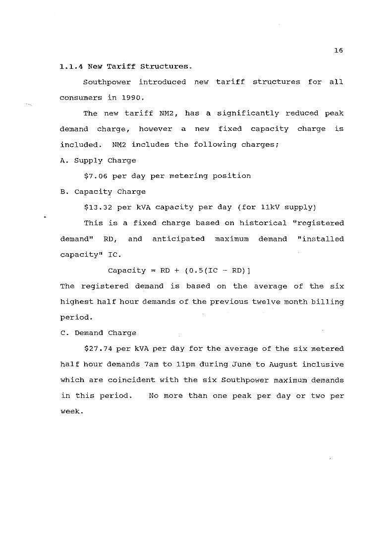
1.1.4 New Tariff structures.
southpower introduced new tariff structures for all
consumers in 1990.
The new tariff NM2, has a significantly reduced peak
demand charge, however a new fixed capacity charge is
included. NM2 includes the following charges;
A. Supply Charge
$7.06 per day per metering position
B. capacity Charge
$13.32 per kVA capacity per day (for 11kV supply)
This is a fixed charge based on historical "registered
demand" RD, and anticipated maximum demand "installed
capacity" IC.
capacity = RD + {0.5(IC - RD)]
The registered demand is based on the average of the six
highest half hour demands of the previous twelve month billing
period.
C. Demand Charge
$27.74 per kVA per day for the average of the six metered
half hour demands 7am to 11pm during June to August inclusive
which are coincident with the six Southpower maximum demands
in this period. No more than one peak per day or two per
week.

17
D. Energy Charge 1) Summer energy (1st October to 30th April)
7.00am to 11.00pm Monday to Friday. 4. 61c/kWh 7.00am to 11.00pm All other days 3.94c/kWh 11.00pm to 7.00am Night rate power 3.38c/kWh
2) Winter energy (1st May to 30th September) 7.00am to 11.00am Monday to Friday 7. 88c/kWh 11.00am to 3.00pm.Monday to Friday 6. 53c/kWh 3.00pm to 9.00pm Monday to Friday 7.88c/kWh 9.00pm to 11.00pm Monday to Friday 6. 53c/kWh 7.00pm to 11.00am All other days 5. 63c/kWh 11.00pm to 7.00am Night rate power 3.38c/kWh
The capacity charge which is based on the consumers
system demand still penalises .consumers with a high peak
demand to base load consumption, although the demand charge
is not as extreme as in the previous tariff.
The capacity charge will always be greater than the
registered demand as the installed capacity is always greater
than actual peak demand. For the University the installed
capacity is about 7.5 MW and demand peak about 2.9 MW, so the
capacity charge will be about 5.2 MW. This reflects the
supply authorities need to charge for its obligation to supply
the maximum demand a consumers installation is rated· for,
rather than the peak demand the consumer is likely to draw.
The consumer is required to pay for having oversized supply
mains capacity f and because of this it would obviously benefit
the consumer to reduce the installed capacity to as low a
value as possible. This could be done by derating the main
line fuses to lower values.

1.2. CAMPUS STEAM HEATING SYSTEM.
1.2.1 STEAM HEATING SYSTEM DESCRIPTION
18
The existing campus steam heating comprises of a central
boilerhouse delivering dry saturated steam at 100 psi (6.89
bar) over the campus via a steam main distribution network in
underground walk through ducts. Figure 1.5 shows the steam
distribution network. Steam mains throughout the site are
150mm diameter, and run full diameter throughout the length
of the underground ducts. The steam mains serving the School
of Engineering are 100mm diameter.
Heat exchangers in each building provide low temperature
hot water for building heating, and domestic hot water
services. Condensate is returned to the boiler feed pumps by
steam traps and condensate return pumps.
Steam is also supplied to the Department of Scientific
and Industrial Research's, Ilam Research Centre in Creyke
Road, and the Ministry of Forestry's, Forest Research Centre.
Both these facilities are charged for steam consumed.
The University of Canterbury Student Union Recreation Centre,
and the University Halls of Residence in Maidstone Road, are
both suplied with medium temperature hot water by inground
"Insapipe" pre insulated heating mains, via heat exchangers
on the main steam heating system.
The central boilerhouse contains two Andersons 200001b/hr
(2.52kg/s) coal fired economic boilers. These were installed
with the building of the science school in the early 1960's.
The School of Engineering, which was opened first on the Ilam
campus, was initially heated by a John Thompson Ltd 8000lb/hr

CAR PARK
------ Lpm~
~
RIVER
FIGURE 1.]
University of Canterbury STEAM DISTRIBUTION MAINS
\
...... 1.0

20
boiler. This is still in service alongside the two larger
Andersons boilers.
Coal feed to the main boilers is by John Thompson chain grate
stokers, and the main boiler feed pumps are Wier steam driven
boiler feed pumps.
Heating System Performance.
All the main boiler plant is in excellent order,
regularly well maintained, and has given reliable service.
It is reasonable to assume that this reliability can be
maintained for a considerable time.
While steam traps are notoriously problematic, and
require continual maintenance attention, they are generally
located in easily accesible locations, and are promptly
attended to when requiring attention. The use of medium or
high temperature hot water, for heating reticulation
throughout campus would be desirable from maintenance, and
energy control and conservation criteria, however the current
record of reliable service of the steam distribution system
would make the economics of converting the existing system
from a maintenance point of view alone questionable.
While the steam distribution system appears to function
satisfactorily, there are problems with the heating system
performance within individual buildings. In some cases the
heating system is unable to achieve the heating levels
required in offices around the campus.
This is confirmed by the high level of electrical demand
experienced on cold winter days I particularly in the mornings. "'-
A recent cold spellAset a new record peak electrical demand
* June 1990

21
of 3.400 MW. Previously peak demands had always been at about
3. 000 MW, suggesting that there could be anything in the order
of about 500 kW of personal electric resistance heaters
scattered around campus.
The main reasons for the heating system problems appear
to be due to changes in building usage over the almost thirty
years of occupancy ( eg Office space modifications occurring
without complementary modification of the heating system ).
A common alteration appears to have been the conversion of
large open plan offices into individual offices, with little
consideration given to changes required to the control of the
heating system. Anomalies in building shell construction and
insulation play an important part in the current performance
shortfalls of the system. Examples of this are ;
until recently the top floor roof of the main library
building was uninsulated.
The Botany I Geology building has a high mass building
construction, but with a poor level of insulation, requiring
a heating system start up time in the morning of about 3. aDam,
six hours before occupancy of the building.
The Engineering school laboratory wi:qgs are partly heated
by uninsulated steam pipes running the length of the
laboratories down the north and south walls, with virtually
no control.
While the above examples are extreme, the experience of . "- .
maintenance staff is that similar problems exist to a degree
in most buildings on campus.
Generally at the time most of the buildings on campus

22
were constructed, standards of building services control
equipment were quite low. Current standards of quality of
control are much higher, and upgrading of control equipment
within buildings is being carried out by the maintenance
department. Overall control of the heating system, and
building services on campus is by a central computerised
energy management and control system, (EMCS). The boilers
are currently manually controlled by boiler attendants, but
an automatic boiler control system is being installed, which
will be supervised by the EMCS.
The increase in the level of comfort that is expected in
buildings now, compared to the levels expected when the
heating system was designed, only serves to make the above
problems more conspicuous to the occupants.
It seems that the heating system components themself are
adequately sized for the loads served, and that the boilers
are providing sufficient steam to the heating system.
Improvements to heating controls, building insulation, and the
overall management of heating services by the energy
management system, should be able to 'improve the performance
of the heating system to a satisfactory standard, as well as
reducing energy consumption.
Sourcej[Interview, D Lloyd Maintainance Dept. August 89]
[Unknown Member of Maintenance Dept., notes,1970'?]

23
1.2.2. STEAM PRODUCTION AND COAL CONSUMPTION.
Figure 1.6 shows the steam demand profiles for the
following typical days.
Winter weekdays and Winter weekends
Summer weekdays and Summer weekends
The demands were developed from boiler steam flow
recorders known to be inaccurate and as such give as good an
indication of actual demands as possible. The winter weekday
demand profile shows the maximum campus heating demand
experienced on cold mid winter mornings.
The other demand profiles give an indication of the year
round heating base load produced by 'domestic hot water demand
and other miscellaneous heat loads.
The campus annual coal consumption shown on Figure 1.7
shows clearly the relationship between heat demand (and
resultant coal consumption) and the seasonal variations in
temperature. It should be noted that the January coal
consumption value is lower than expected as the boilers are
normally shut down for six weeks for maintenance.

~ L
0 z ~ ~ ~ z 1-
~ :x:
FI (-... I I F') -1 7 ~_.., I~ \" .... 1 ... t\l1 1-1 Ei1,1-1 (:; C' .' D
15 -r'4--1 rn----.!d\
'I""" '. " '\ I '.
1 :z , 1
1 Q
9
e 7
e;;
l \. I' ~I;l
l \ ~ \ ..•.
I• lIq., '\ I •
II \
,I 'KJ I 'c I ~
/ \..... WINTER WEEKDAY I ~j--ffi--EEJ--'flj-fil
I \ ~ \
~~---~ .~ ./ ~---m
EI:I---fB--m/ ""-.."l93---ffi
13 -
5
4-3
:2
:;."~'---";~ __ ';;I..._ , WINTER WEEKEND ,. ". r' . . '. -~:""::....--""""---,,;;..._~ .-:-. (jI--,,-4,l--.(:.----I;t------I;!_~~._
. " .. ~ .... ~--.......~--~~--dc... "'_~ -(T--';;I-~T"'-...A!!' ___ ..e.s~",. • . . ........ :a...... SUMMER WEEKDAY
.. .er ..... ~-;O;- ~~_._. . . ....... _r'--=-. ':'" _~"'=----:..,.: • 7-'~~"'~ ll!L~:'-:t!l:--- ,.~. - 7'. ". ,- ,-- SUMMER WEEKEND
, 0 I~--I
o :;: 3 4- 5 ~ 7 e 9 1 '~I l' 1:2 13 14· 15 1 liS 17 1 e , 9 :ZC:1 :2' 22 2~ :24
HOlJR5
FIGURE 1.6 DAlLY STEAM DEMAND PROFILES N ~

L
f---(l)
(()
o o ID
o o to.
o o I.I.l
I I
-
o o .q-
1VO~
E3
NN
Gl
Ct
o
>
f-0 Z
Ir-.O
o [L
-L
il lfji
(;} r:l-..;(
..! r-
::J-'"}
Z
I-::J-'"}
I-;~
~ rt: r-~
I-~ ID
I-Lil I.iI..
25
Z
0 H
~ ID
fQ
ID
0 t:I't
U
Ii) ~
I U
l-
I z 0 "I!! ....
r---. ~ ~ H ~

26
1.3 CAMPUS AIR CONDITIONING.
Cooling Load Distribution.
The university campus comprises many buildings spread
over an area of 20 hectares. While there is a centralised
heating system, the cooling requirements of the campus have
always been met by the installation of individual "current
state of the art" air conditioning plants when the buildings
where constru<;:!ted. The anticipation of a maj or building
program in 1986 provided the initiative for an assesment of
the state of the campus cooling systems. The Ministry of
Works and Development (now Works Corporation of New Zealand)
prepared a report titled "University of Canterbury Chilled
Water Investigations."
The following section is a summary of the campus cooling
systems based on the MOWD Chilled Water Investigations Cooling
load Distribution
A breakdown of cooling requirements on campus is as
follows;
Comfort Air Conditioning (Lecture theatres etc) 66% Library Air Conditioning (Hight, Science, and Eng'g) 14% Computer 8% Specialist 12%
The largest users are the library and lecture theatres
with a combined load of 80% of the total load. Computer
cooling load is due to the computer centre. Remaining cooling
loads are of small capacity and are spread out over many
buildings.
Table 1.2 gives the actual capacity and type of cooling plant
used.

27
TABLE 1. 2 AIR CONDITIONING COOLING LOADS.
BUILDING
Registry
ARTESIAN WATER
kW
James Hight Library 330 Computer Center Modern Languages English Education Arts N Lecture Theatres 317 Arts S Lecture Theatres 92 History Psychology Staff Geog/Psych Lab Block Geography Staff School of Forestry Chemistry/Physics Science Lecture Theatres 460* Botany/Geology Zoology Engineering
-Civil 48 -Elec -Chem -Library -South Lecture theatres -North Lecture theatres -Middle Lecture theatres202
Totals 1499
DIRECT EXPANSION
kW 100
73 12
67 40 37 80 70
13 10
24 1
26
553
CHILLED WATER
kW
134
70
170 224
598
The Science lecture theatres were cooled by an absorption
chiller operating off the steam heating system, however
operating problems present since its installation have meant
that it has not been used in recent years. A lack of suitably
skilled maintenance personnel in New Zealand for absorption
machines is an important factor in this.
Direct expansion air conditioning plant are the most
commmon type on campus. These are typically small units I less
than 10 kW in capacity, which reject heat directly to <the
outside air. Often these are through the wall units which
have been installed well after the building is in service,
which have a high maintenance requirement, and are being

28
installed in increasing numbers as the number of computers
increase on campus.
66% of the total cooling load is due to occupancy, most
of this from the lecture theatres, where cooling will be
required all year round because of the occupancy density.
An important problem in an analysis of the university's
cooling requirements is the lack of information about actual
cooling demand patterns. without a reasonable amount of basic
data on the demands placed on the existing systems no accurate
economic analysis of the benefits of various technical schemes
is possible.
1.4 ENERGY MANAGEMENT AND CONTROL SYSTEM
An energy management system (EMS), is required to control
building services plant operations in order to achieve a
required level of environmental quality, while simUltaneously
minimising energy consumption and operating costs.
The EMS installed by the university's maintenance
department is a Phoenix Energy Management and Control System
(EMCS), produced by Staefa Control System Inc. This system
ties up with the existing services control instrumentation
without compromising the reliability of existing stand-alone
control systems. If any failure on the part of the EMCS
occurs, then the existing services control instruments revert
to local, stand-alone operation. The EMCS operates in a
supervisory manner that optimises the start up and shut down
of the controls in each building on the campus, ensuring that
buildings only come up to temperature when occupancy starts

29
and are shut down before occupancy ceases.
The Phoenix EMCS system allows the use of Direct Digital
Control (DDC) of systems with DDC remote multiplexing
capability
System Architecture and Main Features.
Phoenix is a multi level distributed processing system.
Each programmer supervises specific activities and performs
specific functions. Each programmer typically reports to one
higher level processor and supervises multiple lower level
processors Each processing level is designed to report
failures detected in lower levels and to continue operating
without interruption in the event of a failure of a higher
level.
The main features of the EMCS are;
1. Electrical Demand Limiting.
A power demand monitor gathers electrical demand data
from the university and from the supply authorities system
demand signals (Southpower provides a UHF signal for
notifiable demand peaks) and produces a demand forecast.
2. optimum start and stop Time Determination.
An optimum start time package provides a means of
optimising start up times for the steam heating system for
each building. The package evaluates information such as,
heat build up rates for each building, environmental
conditions, and estimates the start up time that will ensure
the building is at the required temperature at the start of
the occupancy period. similarly the optimum stop time,
allowing for the building I s rate of cooling down, shuts of the

30
heating systems before occupancy finishes so that the minimum
amount of fuel is consumed.
3. Derivation of Data Values.
Important energy values that cannot be determined by a
single sensor can be derived from data from several single
sensors. An example may be the derivation of the value of
enthalpy of fresh air, where the enthalpy may be determined
from a dry bulb temperature sensor and a humidistat. Any
number of sensors may be combined to give averages, maximum
or minimum values, efficiencies, etc.
4. Centralised Time Clock.
The EMCS authorises all time clock functions on the
campus from a central location. This allows out of hours
scheduling of lecture theatres and start up I shut down of
services plant to be easily controlled.
5. Energy Monitoring and Plant Monitoring.
Perhaps the most useful function of the EMCS is its
ability to report and signal an alarm condition on plant
operating status and system energy demand and consumption.
This frees maintenance staff from time consuming plant
checking duties, and enables instant feedback on any
operational or system changes.
Specialised operational programs can be developed using
the EMCS systems "Free Programming Language"
Several software features not associated with energy "
management are also available, eg security monitoring, fire
alarming, planned maintenance scheduling, extensive data
gathering and reporting I and colour graphics for building

31
systems schematics. However as these are not essential
energy management functions and are significant loads on both
the computers memory and operating speed these are not used.
[Staefa Control systems - Phoenix EMCS Prospectus]

32
SECTION 2. ENERGY TECHNOLOGIES FOR CAMPUS
2.1 ELECTRICITY USE REDUCTION OPTIONS.
2.1.1 ELECTRICAL PEAK SHAVING.
A significant part of the electricity supply cost was due
to demand components of the ND6 tariff. A breakdown of annual
electricity cost based on data for the 1988 year is as
follows;
Supply Charge (Fixed Portion) Supply Charge (variable Portion) System Demand Coincident Demand Day Energy (various rates) Night Energy
0.3% 6.6%
22.8% 14.3% 47.7%
8.6%
The combined effect of the demand charges amounted to
43.7% of the annual electricity account, while for the new NM2
tariff controllable demand charges amount to about 18% of
annual charges. These charges are based on the electrical
demand levels at specific times of the day. By generating
electricity on site during coincident, and supply authority
demand charge periods, the consumer may reduce the generally
expensive demand component of its electrical account.' This
is achieved without using the large amounts of. fuel required
to generate the bulk of the daily electrical load.
An analysis of the possible savings due to peak shaving
demand charges follows in this section. The main aims of this
section are;
1. To determine if peak shaving is a viable option.
2. To establish an optimum level of peak shav4.ng
generating capacity, (if it exists).
3. To compare the effects of load reduction to those of
peak Shaving.

33
For this analysis the recoverable heat output of the
generating plant is neglected, as this heat is of
significantly lower thermodynamic and economic value than the
electricity generated. section 2.2, Combined Heat and Power
Generation, examines further the heat and power requirements
of the campus, and shows that extra heat production will be
required in any case as the low grade reject heat from the
generators will be insignificant when compared to the total
campus heating load when the generation plant output matches
the campus electrical load.
The following table shows the actual reductions in
electrical charges resulting from peak shaving. Charges are
based on the consumption data from electricity accounts for
the period 21 July 1988 till 18 August 1988 and as such
reflect the effects of the older ND6 tariff.
TABLE 2.1 ELECTRICAL PEAK SHAVING SAVINGS Amount of peak shaved OMW IMW 2MW 3MW
Supply Charge 28 days $193 $193 $193 $193 Supply Charge Demand $7200 $7200 $7200 $7200 System Demand Charge $12532 $8355 $4175 $0 coincident Demand Charge $16425 $10950 $5475 $0 winter Energy.
7.00 - 11 00 Weekday $11150 $11150 $11150 $11150 11 00 - 15.00 Weekday $11716 $11716 $11716 $11716 15.00 - 21.00 WeeJs.day $16665 $16665 $16665 $16665 21.00 -.23.00 Weekday $2704 $2704 $2704 $2704 Weekend Day $5884 $5884 $5884 $5884 Night Rate ~5442 ~5442 ~5442 ~5442
Total Charges. $89911 $80259 $70604 $60954
The calculated peak shaving charge reductions are the
maximum that can be achieved for the installed peak shaving
generating capacity. Fuel, capital, and maintenance costs
have been neglected in this analysis as peak shaving
generation involves operation only during the short demand
34
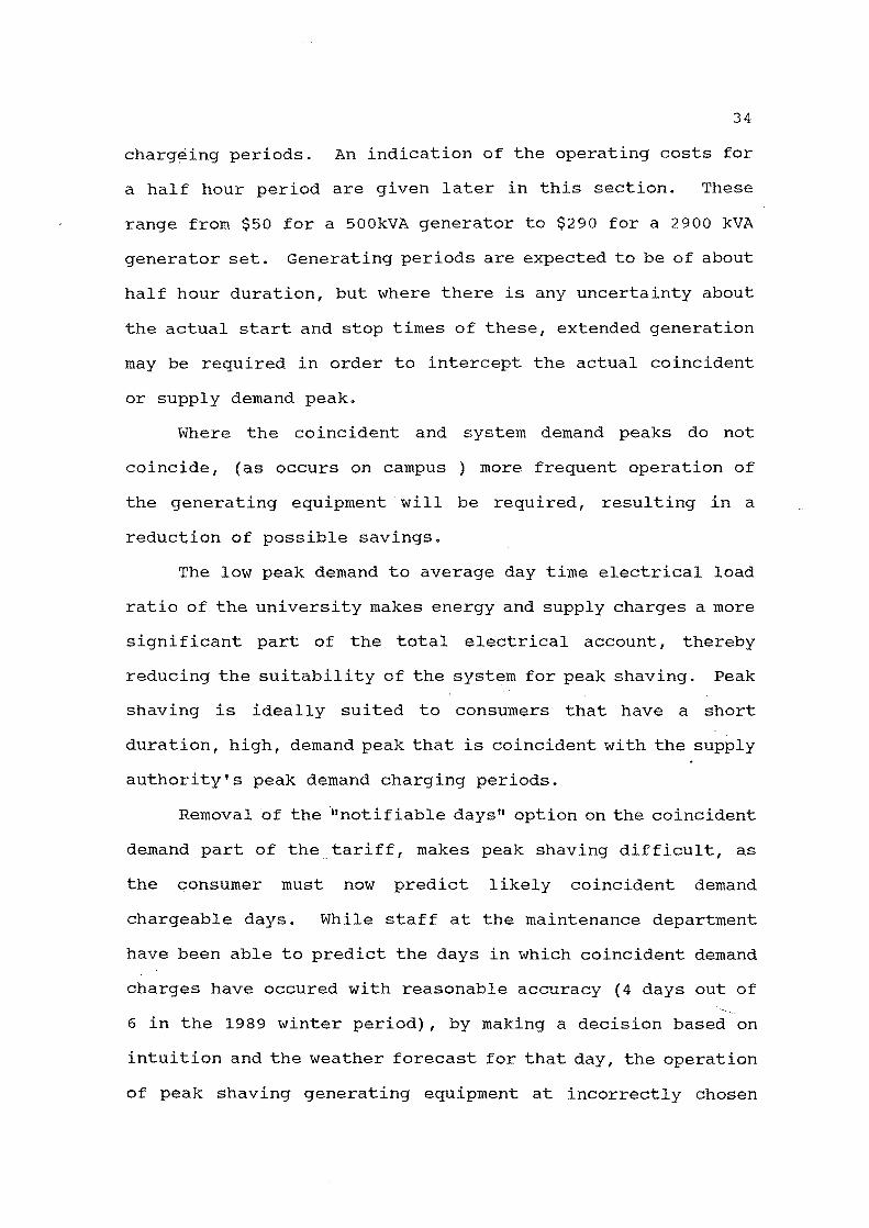
chargeing periods. An indication of the operating costs for
a half hour period are given later in this section. These
range from $50 for a 500kVA generator to $290 for a 2900 kVA
generator set. Generating periods are expected to be of about
half hour duration, but where there is any uncertainty about
the actual start and stop times of these, extended generation
may be required in order to intercept the actual coincident
or supply demand peak.
Where the coincident and system demand peaks do not
coincide, (as occurs on campus ) more frequent operation of
the generating equipment will be required, resulting in a
reduction of possible savings.
The low peak demand to average day time electrical load
ratio of the university makes energy and supply charges a more
significant part of the total electrical account, thereby
reducing the suitability of the system for peak shaving. Peak
shaving is ideally sui ted to consumers that have a short
duration, high, demand peak that is coincident with the supply
authority's peak demand charging periods.
Removal of the '''notifiable days" option on the coincident
demand part of the .. tariff, makes peak shaving difficult, as
the consumer must now predict likely coincident demand
chargeable days. While staff at the maintenance department
have been able to predict the days in which coincident demand
charges have occured with reasonable accuracy (4 days out of
6 in the 1989 winter period), by making a decision based on
intuition and the weather forecast for that day, the operation
of peak shaving generating equipment at incorrectly chosen

35
times would soon eliminate the savings achieved.
Peak Shaving System Costs.
Because of the uncertainty of the frequency and duration
of operation of a peak shaving plant, accurate assessment of
operating costs becomes difficult. However a basic summary
of the capital and operating costs of a range of peak shaving
plants is given in the following table;
PEAK SHAVING PLANT COSTS.
Generator Generator Unit cost, Capacity Installed Half Hour
Capital cost operation
500kW $195,000 $50 800kW $255,000 $80
1300kW $420,000 $130 1600kW $465,000 $160 2900kW $885,000 $290
The above costs are based on the following;
1- Capital costs are for Diesel generator sets, Dual fuel
or Gas engines are approximately twice as expensive.
2. unit cost for half hour operation based on Diesel cost of
$0.67 per litre giving a electricity production cost of $0.20
per kWh.
j. Installed cost of the generator set is taken as 1.5 times
the capital cost. [SARGEANT W. ]
36
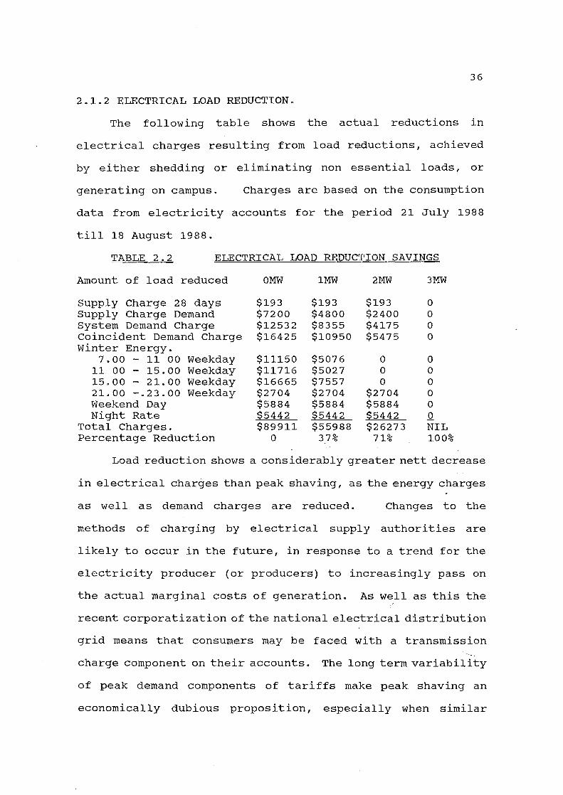
2.l.2 ELECTRICAL LOAD REDUCTION.
The following table shows the actual reductions in
electrical charges resulting from load reductions, achieved
by either shedding or eliminating non essential loads, or
generating on campus. Charges are based on the consumption
data from electricity accounts for the period 21 July 1988
till 18 August 1988.
TABLE 2.2 ELECTRICAL LOAD REDUCTION SAVINGS
Amount of load reduced OMW IMW 2MW 3MW
Supply Charge 28 days $193 $193 $193 0 Supply Charge Demand $7200 $4800 $2400 0 System Demand Charge $12532 $8355 $4175 0 Coincident Demand Charge $16425 $10950 $5475 0 winter Energy_
7.00 - 11 00 Weekday $11150 $5076 0 0 11 00 - 15.00 Weekday $11716 $5027 0 0 15.00 - 21. 00 Weekday $16665 $7557 0 0 21.00 -.23.00 Weekday $2704 $2704 $2704 0 Weekend Day $5884 $5884 $5884 0 Night Rate ~5442 ~5442 ~5442 Q
Total Charges. $89911 $55988 $26273 NIL Percentage Reduction 0 37% 71% 100%
Load reduction shows a considerably greater nett decrease
in electrical charges than peak shaving, as the energy charges
as well as demand charges are reduced. Changes to the
methods of charging by electrical supply authorities are
likely to occur in the future, in response to a trend for the
electricity producer (or producers) to increasingly pass on
the actual marginal costs of generation. As well as this the
recent corporatization of the national electrical distribution
grid means that consumers may be faced with a transmission
charge component on their accounts. The long term variability
of peak demand components of tariffs make peak shaving an
economically dubious proposition, especially when similar

37
savings could be expected from reductions in electrical load
from improved electrical usage management. This is shown
clearly by the reduction in the potential for peak shaving
associated with the introduction of the NM2 tariff and its
lower demand component.
The fact that significant reductions in electricity
consumption could be achieved through the continued
installation of modern high efficiency electrical fittings
with optimum control, makes the installation of peak shaving
generating equipment economically questionable. By making
operational changes to the running of the university
reductions in energy use can be made, however this may
ultimately affect the effectiveness of the university's goals
of teaching and research.

38
2.2. COMBINED HEAT AND POWER GENERATION.
Combined Heat and Power (CHP) production is widely
recognised as an efficient method of simultaneously satisfying
electrical and heating requirements for a variety of
industries, public institutions, and residential schemes.
While many different types of CHP scheme exist, the
thermodynamic principle of minimising irreversible losses by
utilising high grade heat for generating work, and low grade
"reject" heat for useful heating, from a single heat source,
is a common feature.
From an energy conservation point of view CHP provides
a means of supplying energy services to society with a
considerably lower drain on fossil fuel stocks. A 1989 report
The Potential For Cogeneration in New Zealand [Ministry of
Energy] concludes:
"There is considerable potential for further cogeneration in New Zealand; as much as 300 GWh/year at a cost of
12c/kWh (the current Electricorp long run marginal cost 0 f production) or less. The fuel efficiency for this level of cogenerated energy is expected to range from 65% to ~ ie between two and three times the fuel efficiency 0 f Electricorp (thermal) generating plant."
Despite this apparently optimistic conclusion the level
of CHP output in New Zealand is still quite low. The main
cogenerators are the dairy and the pulp and paper industries.
CHP production for institutions is at a very low level, and
schemes that are in operation are marginal in their cost
effectiveness. There would appear to be few technical problems
associated with CHP plant. Both gas turbine and steam turbine
(currently producing most of the cogenerated energy in New
Zealand) alternator sets are available in a wide variety of

sizes and configurations with good records of reliability.
Factors influencing CHP feasibility.
39
1. Energy costs. Both the relative price differences
between different fuel sources and uncertainty over the future
trends in fuel prices, affect the feasibility of various CHP
schemes, and make reliable assesment of benefits difficult.
In New Zealand with a large supply of cheap hydro based
electricity, the ability of any other generating system to
produce electricity competitively is limited.
2. High capital costs of CHP plants make reasonable rates
of return on investment hard to attain, and increase the level
of financial risk to a CHP user, making other less expensive
energy strategies more attractive.
3. Both heat and power load densities need to be quite
high in order to keep energy distribution costs to a minimum.
Proximity of the heat load to the power generating source is
also important.
4. The ability to purchase standby electricity in the
event of break down, without excessive financial penalty, and
the ability to sell excess power at reasonable price, improve
the feasibility of a CHP plant dealing with unmatched or
varying loads.
5. Variable heat and power loads, especially where these
occur independantly, make both design and operation of CHP
plant uncertain.
2.2.1. CHP PLANT CHARACTERISTICS.
Steam Turbines.
40
This is the most common CHP plant in New Zealand, capable
of being fired on coal, gas, wood, or waste fuels, high
pressure steam (typically at 20 to 60 bar) passes through a
turbine to a lower pressure steam process load.
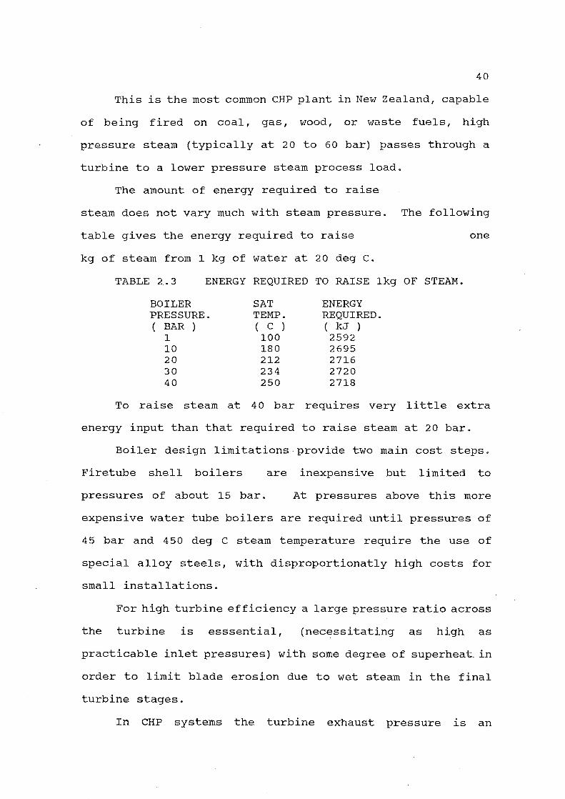
The amount of energy required to raise
steam does not vary much with steam pressure. The following
table gives the energy required to raise one
kg of steam from 1 kg of water at 20 deg C.
TABLE 2.3 ENERGY REQUIRED TO RAISE lkg OF STEAM.
BOILER PRESSURE. ( BAR )
1 10 20 30 40
SAT TEMP. ( C ) 100 180 212 234 250
ENERGY REQUIRED. ( kJ ) 2592 2695 2716 2720 2718
To raise steam at 40 bar requires very little extra
energy input than that required to raise steam at 20 bar.
Boiler design limitations-provide two main cost steps.
Firetube shell boilers are inexpensive but limited to
pressures of about 15 bar. At pressures above this more
expensive water tube boilers are required until pressures of
45 bar and 450 deg C steam temperature require the use of
special alloy steels, with disproportionatly high costs for
small installations.
For high turbine efficiency a large pressure ratio across
the turbine is esssential, (necessitating as high as
practicable inlet pressures) with some degree of superheat in
order to limit blade erosion due to wet steam in the final
turbine stages.
In CHP systems the turbine exhaust pressure is an

41
important consideration. Unlike large power generating
condensing turbines with turbine outlet conditions close to
atmospheric temperature the heat or process load temperature
requirements can considerably raise turbine outlet conditons.
As a drop in exhaust pressure can give an increase in turbine
output greater than that from an equal increase in turbine
inlet pressure this is particularly important.
The following table gives turbine work output, and work
to heat ratio as a function of exhaust pressure.
TABLE 2.4 EFFECT OF INPUT/EXHAUST PRESSURES ON TURBINE OUTPUT
TURBINE TURBINE WORK WORK / INLET EXHAUST OUTPUT HEAT PRESSURE PRESSURE RATIO ( BAR ) ( BAR ) (kJ/kg) ( Q/W
40 10 315 0.13 40 7 378 0.16 40 2 588 0.20 40 1 684 0.32
See also Appendix A The campus steam heating system operates with a boiler
pressure of 100 psi (6.9 bar), which would form a severe
limitation on turbine performance.
Turbine internal efficiency is also an important factor.
"Although it is impossible to generalise due to the large number of permutations of steam pressures, temperatures and flows possible through a given turbine, a high speed geared machine is usually more efficient than a direct coupled machine for the smaller powers and exhaust volume flows. The gain in power more than offsets the gearing losses." [Valentine]
Most small turbines operate at about 7000 to 12000 rpm
and require gearboxes.
Back Pressure and Pass Out Turbines.
Table 2.4 in the previous section gave the theoretical

42
heat to work ratio for turbines operating with different
exhaust pressures. The operating efficiency of a back
pressure turbine can be optimised by selecting a back pressure
such that the heat/work demand characteristic of the load is
matched to the turbine. In order to use a back pressure
turbine on the existing campus steam system a 7 bar exhaust
pressure limit will be placed on the turbine as this is the
pressure at which steam is currently produced for the campus
heating system. This will produce a work/heat output ratio
of 0.16 which is likely to be too low, as the typical
work/heat ratio during daytime for the campus varies from 0.2
in summer weekends, to about 0.3 in winter. This means that
at 7 bar exhaust pressure, supplementary boiler heating will
be required throughout the year if the electrical load is
matched. However if the campus heat load is matched by the
CHP plant excess electricity will be available for sale. The
work/heat load ratio of the campus varies considerably
throughout the day as well as throughout the year, and at
certain times of the year a better match between loads and
turbine outputs will occur.
By lowering the exhaust pressure to 2 bar the turbine
work/heat ratio will be close to 0.2 and will more closely
match the campus work/heat load ratio. This will however put
a maximum temperature limit of about 115 deg.C on the campus
heating system. By converting the campus heating system to
medium temperature hot water heating rather than steam this
could be achieved, using a heat exchanger between the steam
system and hot water heating system. This would still not

43
optimise the turbine for any work/heat ratio other than the
design one of 0.2. As the campus heat and electricity loads
both vary considerably and independantly the efficiency of a
back pressure turbine would be compromised frequently.
At this stage the desirability of using of a pass out or
extraction turbine becomes apparent. Here steam is first
passed through a high pressure (HP) turbine stage, to the heat
or process load operating pressure, where it is either bled
off to the heating load or further expanded through a low
pressure (LP) condensing turbine stage. This significantly
improves the turbine performance as the LP stage allows
expansion of the non bled steam into the wet steam region down
to pressures limited by the condensing medium's temperature.
A pass out turbine for the campus would bleed steam at 7 bar
to the heating system, however converting the heating system
to MTHW operation would improve the turbine performance even
further as the HP turbine stage would expand the full steam
mass flow to a lower bleed pressure. The pass out turbine
also allows much greater flexibility in matching the turbine
heat and work outputs to the work/heat ratio of the load. Fig
2.3 shows the range of work/heat ratios that can be covered
without importing or exporting heat or power for the campus.
While the need to match turbine characteristics to load
is important, attempting to neither import or export heat or
power may not be the overall most efficient use of the plant
or fuel. As the electrical output is the most valuable,
maximising this output (rather than losing potential work in
incompletely expanded steam) and selling extra electricity is

44
more efficient than operating at a lower efficiency for the
sake of achieving a close match of loads to turbine output.
For the university this would mean sizing the turbine to
match peak heating loads and selling any extra electricity
resulting. This shows that the ability to sell excess power
without penalty is an important factor in the decision to
install a CHP plant.
GAS TURBINES.
While steam turbines have traditionally been the main
prime mover for thermal electricity generation, the rapid
start up ability of gas turbines has made the gas turbine
popular as a low capital cost peak load demand generator. In
New Zealand, Electricorp has several gas turbine based peak
load plants, ie Otahuhu, Stratford, and Whirinaki.
For CHP schemes the gas turbine is particularly sui table
as the heat input not converted to shaft power is available
as a high temperature exhaust gas (cf the low pressure low
temperature exhaust steam from a steam turbine) which can
readily produce a high grade process output. Compared to a
diesel or dual fuel oil/gas engine where about 30% of the fuel
input is rejected as low grade cooling water, this is quite
significant. Both gas turbines and oil/gas engines produce
an oxygen rich exhaust which can be further burnt with fuel
to produce steam, this will however reduce the overall fuel ~
utilisation factor as the extra fuel burnt in the boiler
produces no work output.
Table 2.5 shows that generally gas turbine thermal

45
efficiency falls between that of a condensing steam turbine
and back pressure turbine.
TABLE 2.5 CHP PLANT TYPES AND THEIR EFFICIENCIES.
GENERATOR TYPE
Gas Turbine Condensing ST Back Press ST Pass Out ST Gas/oil Engine
WORK OUTPUT
0.3 0.4 0.25 0.38 0.36
USEFUL HEAT OUTPUT
0.55 0.0 0.6 0.1 0.3
ENERGY UTILISATION FACTOR
0.85 0.4 0.85 0.48 0.66
[after Horlock]
However in CHP schemes thermal efficiency alone is not
the most important factor in determining the suitability of
a prime mover.
The ability of a CHP plant to maintain a high efficiency
when following a wide range of varying electrical and heat
loads is perhaps more important. This is especially important
in the case of the university campus where heat requirements
vary from 14.5 MW to virtually'nothing and electrical loads
vary from 2.9 MW to 0.5 MW.
"The part load performance is also affected-by the cycle chosen and by the method by which the (gas turbine) shafts are controlled. For instance a single shaft machine controlled to operate at constant speed for power generation tends to have poor part load performance, as at low speeds the compressor is forced to operate at full speed at part of its characteristic where it is not too efficient " [Craig]
An advantage of the gas turbine at part load operation
is that if little or no heat load is r~quired the turbine
exhaust can bypass the heat recovery boiler to an exhaust
stack, whereas a steam turbine always requires all the steam
to be condensed before returning to the boiler feed pumps,
requiring in some cases a considerable condenser and cooling
46
tower.
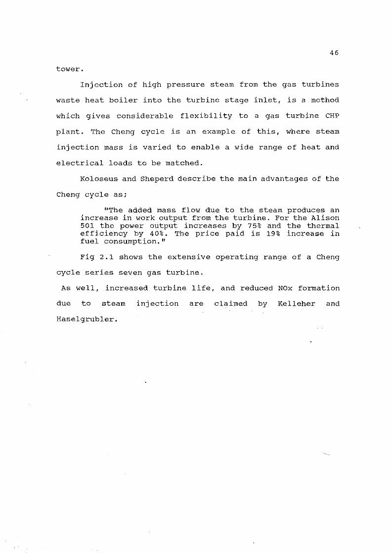
Injection of high pressure steam from the gas turbines
waste heat boiler into the turbine stage inlet, is a method
which gives considerable flexibility to a gas turbine CHP
plant. The Cheng cycle is an example of this, where steam
injection mass is varied to enable a wide range of heat and
electrical loads to be matched.
Koloseus and Sheperd describe the main advantages of the
Cheng cycle as;
"The added mass flow due to the steam produces an increase in work output from the turbine. For the Alison 501 the power output increases by 75% and the thermal efficiency by 40%. The price paid is 19% increase in fuel consumption."
Fig 2.1 shows the extensive operating range of a Cheng
cycle series seven gas turbine.
As well, increased turbine life, and reduced NOx formation
due to steam injection are claimed by Kelleher and
Haselgrubler.

6
5
,.-.. 4 ~ '-"
+-l
5. +-l
(5 r-I
Ci:! U
• .-1 ~ +-l U OJ
r-I r:il
3
2
1
o o
Turbine at part
Stearn injection with supplementary firing
* with stearn injection Turbine peak output without stearn injection
~'" o .-<$'
4Y • '0-tO
~'\)Y «"-$>
.0'0-",y
• eF.I . '0-)
!$>Y ",to'?f
<0
5 10
Supplementary firing in waste heat boiler
FIGURE 2.1 CHENG CYCLE OPERATING RANGE
15 Steam Output (kg x 1000)
>t>. -...)

48
2.2.2. Assessment of feasibility of CHP for Campus.
Design Heat and Power Loads.
An accurate estimate of the heat and electrical loads
under which a CHP scheme will operate is essential to the
sound analysis of the thermodynamic and economic performance
of the CHP system.
Most industrial plants and institutions have complex,
varying, heat and power load profiles, determined by the
operating and environmental conditions. Methods for
measuring the heat and power loads vary in complexity and
accuracy, with more frequent measurements being required for
continuously varying complex loads.
The simplest analysis involves taking a yearly average
of heat and power loads and energy consumption, however this
crude approximation is only suitable for the simplest initial
feasibility study. Taking monthly averages of daily loads
gives a more accurate assessment, reflecting diurnal and
yearly load variations, resulting in 12 monthly average load
profiles. If the actual hourly loads are determined from
historical records the most accurate analysis of operating
conditions can be built up, and a accurate ass.essment of
actual operating costs and savings can be made. However the
disadvantage of this is the large number of calculations
required to produce this highly accurate result.
Bonham in a discussion of Ruston Gas Turbines TESOS
(Total Energy Simulation Optimisation Study) computer based
CHP plant simulator states:
"-we have found by experience that a sufficiently accurate evaluation (of a CHP schemes performance) can

49
be made by considering only four typical operating days, namely
A typical winter production day, A typical summer production day, A typical winter non-production day, A typical summer non-production day,"
[P BONHAM]
In the case of the university campus the above method of
analysing the CHP loads is particularly appropriate, as the
winter heating season almost coincides with the university
term from March to October, and the typical daily loads are
reasonably constant throughout the summer and winter periods.
This method should give a sufficiently accurate assessment of
the annual operation of the CHP plant, without requiring an
excessive number of calculations.
A spreadsheet based load analysis program has been
developed to enable a reasonably accurate estimate of the
costs and benefits likely from the installation of a CHP plant
on the campus. The following features are included:
1) The effects of variations in simUltaneous daily heat
and electrical loads are taken into account.
2) Required amounts of heat and/or electricity to be
imported or exported resulting from imbalances between
CHP outputs and load requirements are given.
3) Plant operation in two modes:
a. CHP plant satisfies electrical demand, heat may
need balancing.
b. CHP plant satisfies heat demand, electrical l<Jad
may need balancing.
4) Variations in plant thermal efficiency due to part
load operation are taken into account.

50
5) operating costs, including fuel and maintenance
costs, and final heat and electricity output unit
charges produced.
The CHP plant is assumed to operate continuously
throughout the year, in order to maximise savings and return
on capital cost, although in practice, operation in summer may
not be economical.
Electrical tariff energy and demand charges are not
included in the analysis for simplicity.
2.2.3. CHP SCHEME ANALYSIS RESULTS.
The following pages include summary sheets from the CHP
analysis spreadsheets as well as details of the thermodynamic
characteristics and economic factors used in the analysis.
A complete example of one of the spreadsheets with explanatary
notes is included in appendix D.
1. BACK PRESSURE TURBINE, 7BAR EXHAUST PRESSURE.
As no performance data relating to a specific production
back pressure turbine was available, a performance model was
developed based on an analysis of steam consumption of back
pressure turbines by Kearton. See KEARTON 1964. The
relationship between shaft power output, and total steam
consumption is given based on the following design conditions:
Turbine steam inlet condition Turbine back pressure Maximum power output Turbine isentropic effy.
40bar 7bar 3MW 0.9
@ 400deg C
The relationship between inlet steam flow rate I and
electrical load is shown on Figure 2.2 and is based on the

10 kg/s 20
I I
f I
f f
I
, , I ,
15 I
~10 5kg/s OJ ..., (fl
OJ C .,.,
.0 ,.. ;:l
H
5
a a
f
I
I
I
I
/
1 2
I
I
I
I
3 Turbine work output(Mln
FIGURE 2.2 BACK PRESSURE TURBINE STEAM CONSUMPTION

52
calculations in Appendix A.
In realising this performance model on the CHP analysis
spreadsheet, the back pressure turbine steam consumption is
determined from the campus heat load, and simultaneous
electrical load from the campus electrical load. The
following relationship for turbine steam consumption is based
on linear equations relating steam consumption to coincident
heat and electrical loads.
Qin = 3.06MW + 6.28 * Wout MW
This is the function used to determine the thermodynamic
performance of the back pressure turbine CHP plant when
following the electrical load.
Similarly the analysis for the CHP plant following the
heat load uses the linear heat load to steam consumption
relationship, here the efficiency function is given by:
Qin 1.189*Qout - O.57MW/HW
For derivation refer Appendix A.
Economic analysis of the CHP plant is based on the
results of the thermodynamic performance of the turbine, and
the following economic factors:
Capital costs. (source Ministry Boiler (48 bar 450 c )
Cost Installation
Turbine / Alternator
of Energy 1989)
Cost Installation
Maintenance costs. Total
Boiler (5% capital cost / ann.) Turbine / alternator
Fuel costs. (University of Canterbury) Coal ($88 / tonne @ 28MJ / kg LCV)
$M4.4 $M1.0
$370,000 $510,000 $M6.3
$220,000 $70,000
$ 11/MWh

53
Electricity (Ann. mean cost) $90/MWh
No attempt at detailed economic analys made, only
a basic annual CHP plant operating cost is developed and
compared to the present energy supply arrangement costs.
The following two pages sumarises the results of the CHP
analysis spreadsheet

BACK PRESSURE TURBINE FOLLOWING ELECTRICAL LOAD.
PLANT NAME BACK PRESS TURB Th Effy function E = 9.4 + 1.5 *(EL FUEL: TYPE COAL Fuel Cost $/MWh Rated work output 3 MW Electy cost $/MWh Heat cost $/MWh; 11.00 Maintenance $/ann Capi tal cost $; 6300000.00 Useful/rejectheat
PERFORMANCE RESULTS SUMMARY
Annual Steam MWh 34175.44 Stm.Charge.$/MWh Annua 1 Elect MWh 9471.28 Elec.Charge.$/MWh
Ann CHP Qin MWH 89515.64 Ann CHP Qin cost 2567895.45
CHP Qout MWh 61193.53 CHP Qbal M\.tJH CHP Qout cost $ 1652225.19 CHP Qbal cost$
CHP Wout MWh 9471.28 Annual CHP cost $ CHP Wout cost $ 871357.76 Current Ann.Cost
Profit
Mean Th Effy 10.58 Hours Operation at Rated Output.
EUF cycle 0.79 EUF system 0.7'"
11.00 92.00
290000. 1 .00
27.00 92.00
-23444.73 -670519.16
3132376.30 1251009.00
-1881367.30
3021 .14
\.n .l:'-

BACK PRESSURE TURBINE FOLLOWS HEAT LOAD
PLANT NAME FUEL: TYPE
BACK P. TURBINE COAL
Th Effy function Qin=1.189*(Qout)-0 Cost $/MWh 11.00
Rated work outputELEC. 3MW Elect'y cost $/MW 90.00 Heat cost $/MWh= 11.00 Maintenance $/ann 290136.00 Capital cost $; 6300000.00 Useful/waste heat 1.00
PERFORMANCE RESULTS SUMMARY.
Ann ua 1 Steam MWh 37748.80 Stm.Charge.$/MWh AnnLla 1 Elect MWh 9475.60 Elec.Charge.$/MWh
CHP Qin MWH 39696.32 CHP Qin cost $ 436659.56
CHP W'OLlt MWh 1947. CH," Wba 1 MWH -7528.08 CHP Wout cost $ 175277.09 CHP Wbal costS 677526.91
HOLlr's op era t ion Mean Th Effy 0.05 at rated output 649.17
EUF plant 1 .00 Annual CHP cost $ 2349322.47 EtJF system 1.00 Current ann. cost 1251009.00
Profit -1098313.47 V1 V1

56
2. PASS OUT TURBINE, 7BAR PASS OUT PRESSURE.
As no performance data relating to a specific production
pass out turbine was available, a performance model was
developed based on an analysis of steam consumption of passout
turbines by Kearton. See KEARTON 1951. The relationship
between shaft power output, pass out bleed steam, and total
steam consumption given based on the following design
conditions:
Turbine steam inlet condition Pass out bleed pressure Turbine exhaust pressure Maximum power output Maximum power - no pass out
Maximum pass out steam load Turbine isentropic effy.
40bar @ 400deg C 7bar
O.lbar 3MW 1.6MW
15MW 0.9
(Summer peak elec. )
Two cases are developed, Full extraction, and No
extraction of pass out steam in the analysis which is given
in appendix B
The resulting inlet steam,. pass out steam and electrical
power relationship is shown on Figure 2.3. Although turbine
design conditions will be different, the full extractio.n steam
consumption line on Figure 2.3 shows the steam consumption of
a back pressure turbine with exhaust pressure of 7 bar.
Likewise the no extraction line shows the steam consumption
of a condensing turbine with a condenser pressure of 0.1 bar.
The ability of a pass out turbine to perfectly match any work
/ heat ratio between these two turbine operating extremes by
controlling passout steam flow can be seen from this diag~am.
Theoretical turbine electrical efficiency curves and pass
out bleed steam rates are superimposed and show the improved

57
work efficiency of the second stage condensing turbine, and
the wide range of work / heat ratios the pass out turbine can
accomodate.
In realising this performance model on the CHP analysis
spreadsheet, the pass out bleed steam flow is determined from
the campus heat load, and simultaneous electrical load from
the campus electrical load. The following relationship for
turbine steam consumption is based on linear equations
relating steam consumption to passout steam flow and
electrical load.
Qin =1.12 + (Qout * 0.684) + (Wout * 2.433) MW
This equation is the turbine efficiency function used
in the CHP analysis spreadsheet to determine the thermodynamic
performance of the pass out turbine CHP plant.
Economic analysis of the CHP plant is based on the
results of the thermodynamic performance of the turbine, and
the same economic factors as used for the back pressure
turbine. In many cases a turbine manufacturer I s -back
pressure turbines will be pass out turbines with blanked off
pass out steam bleed points.
The following .. page sumarises the results of the CHP
analysis spreadsheet

3 r:: 0
',-l .u
~ crJ r:: 0 CJ
E C\l Q) .u crJ
Q)
r:: ',-l ,t::l
\..j ;:l
H
20 8 kg/s
15 .6 kg/s
10 ,4 kg/s
5
I
/
I I
I
, "
I
I
, I
I ,
" / ,/ 4'
" " /,
I
" " " I " " " " , " "
/" / '
" " " "
I
, ,/
./
, I
/' /'
" /'
" I .
" "
" "
/
" "
o ;-------------~----------_.------------~ o 1 2 3
Turbine work output(MW)
FIGURE 2.3 PASS OUT .TURBINE STEAM CONSUMPTION

(
PASS OUT TURBINE - MATCHED LOADS.
PLANT NAME FUEL: TYPE
PASS OUT TURBINE COAL
Th Effy function Qin=(Qo*0.684)+1.1 Cost $/MWh 11.00
Rated work outputElec. 3MW Elect'y cost $/MW 90.00 Qin cost $/MWh; 11.00 Maintenance $/ann 290000.00 Capital cost $ 6300000.00 Useful/Qout Heat 0.95
PERFORMANCE RESULTS SUMMARY.
Annual Steam MWh Annual Elect MWh
Ann CHP Qin MWH Ann CHP Qin cost
Qcond CHP Condo Capty.
Mean Th Effy
EUFc:ycl e EUFsystem
37748.80 Stm.Charge.$/MWh 9475.60 Elec.Charge.$/MWh
59066.31 649729.45
11841.91 Ann CHP cost $ 2.83 Current Ann cost
Profit
0.15 Hours Operation
0.80 0.80
1884729.45 1251009.00 -633720.45
3158.53
V1 '-D

60
3. GAS TURBINE, WASTE HEAT RECOVERY BOILER.
Although natural gas is not available in Canterbury in
sufficient quantities to supply a CHP instalation, because of
its importance as a CHP fuel, the relatively low capital cost,
and high temperature heat output of gas turbines, a model was
produced in order to give a comparison between gas and coal
fired CHP systems.
For the Gas turbine analysis the performance
characteristics of a production Alison 501k gas turbines are
used.
The economic performance of the gas turbine is based on
the thermodynamic performance and the following economic
factors:
Gas Turbine capital costs.
capital costs. (source Ministry of Energy Gas Turbine (inc 3MW alternator)
Cost Installation
Heat Recovery boiler Cost Installation
Total
Maintenance costs (annual)
Fuel Costs (source Wellington Gas Co) (Monthly billing)
$15.1/GJ for 1st 40GJ ($S4/MWh) $11.6/GJ for next 60GJ ($42/MWh) $7.95/GJ for balance ($28/MWh) Mean Ann. Gas cost:
1989)
$M2.3 $510,000
$Ml.2 $88,000 $M4~1
$40400
$Ml.269 = $28.7/MWh 44998 MWh
(This assumes annual fuel consumption of 44998 MWh)
Electricity $90/MWh
The thermal efficiency functions for the gas turbine are
assumed to be linear, however in practise as the specific fuel

61
consumption increases non linearly, and as power output drops
the linear estimate will provide a more conservative value for
turbine heat input.
The thermal efficiency function for the gas turbine
following the electrical load is;
Effy = 14% + 4.67% * (Wout MW)
For the case of the gas turbine following the heat load
two gas turbines are assumed in the analysis, as one Alison
SOlk gas turbine alone is incapable of supplying the maximum
campus heat load. The thermal efficiency function for the
gas turbine following the heat load is;
Effy 7.32% + 1.19% * (Qout MW)
This assumes that the two gas turbines will operate in
parallel although in practise they will probably be staged
when the heat demands are sufficiently high to require both
turbines to operate.
The analysis from which these functions were produced is
detailed in Appendix C Gas Turbine Performance Calculations.
The following pages summarise the results of the gas
turbine CHP analysis spreadsheets.

GAS TURBINE FOLLOWS HEAT LOAD
PLANT NAME 2x ALLISON 501-K Th Effy function Effy=7.32+1.19*(Qo FUEL: TYPE NAT'L GAS Cost $/MWh 11.00 Rated work outputELEC. 3MW Elect'y cost $/MW 90.00 Heat cost $/MWh; 27.00 Maintenance S/ann 80800.00 Capital cost $; 5200000.00 Useful/waste heat 0.79
PERFORMANCE RESULTS SUMMARY.
Annual Steam MWh Annual Elect MWh
CHP Qin MWH CHP Qin cost $
CHP WOLtt MWh CHP Wout cost $
Mean Th Effy
EUF plant EUF system
37748.80 Stm.Charge. 9475.60 Elec.Charge.$/
46228.43 508512.72
6289.63 CHP Wbal MWH 566066.58 CHP Wbal costS
Hours operation 0.14 at rated output
0.95 Annual CHP cost $ 0.96 Current ann. cost
Profit
-3185.97 286737.42
1048.27
1656050.13 1251009.00 -405041.13
a-.. N

GAS TURBINE FOLLOWING ELECTRICAL LOAD.
PLANT NAI"IE FUEL: TYPE Rated work output Heat cost $/MWh; Capital cost $;
ALLISON 501-K /L GAS
3 MW 27.00
2600000.00
Th Effy function Fuel Cost $/MWh Electy cost $ Maintenance $/ann Useful/rejectheat
PERFORMANCE RESULTS SUMMARY
Annual Steam MWh 34175.44 Stm.Charge.$/MWh Annual Elect MWh 9471.28 Elec.Charge.$/MWh
Ann CHP Qin MWH 49389.03 Ann CHP GHn cost 1419471 .83
CHP Qout MWh 29654.01 CHP Qbal CHP Qout cost $ 800658.25 CHP Qbal cost$
CHP Wou t MWh 9471.28 AnnLtal CHP cost $ CHP Wout cost $ 871357.76 Current Ann.Cost
Profit
Mean Th Effy 19~18 Hours Operation at Rated Output.
EUF cycle 0.79 EUF system 0.79
(ELEC LOAD)*4.67+1 28.75 92.00
40400.00 0.79
27.00 92.00
8094.79 231511.02
2081382.85 1251009.00 -830373.85
3021 .14
(]'\ w

64
Discussion of CHP Analysis Results
The performance of the CHP plants has been determined
from theoretical plant operation models, and for the purposes
of this feasibility study have been sufficiently accurate,
however for improved accuracy, actual plant performance
patterns should be used. Further accuracy would be achieved
by using monthly load profiles rather than the four
winter/summer daily load profiles. This would better show the
effects on the plant of seasonal load variations. The load
patterns for the steam system were taken from boiler steam
flow charts known to have ina7~racies that may have
overestimated the actual steam flow, however the totalled
annual steam load equalled the actual annual steam production
of the system.
Table ~ .. 6 summarises the main cost / benefit factors of
the five CHP systems ranked in order of annual savings due to
CHP operation instead of the existing separate electrical and
heat supply.
TABLE 2.6
CHP SYSTEM
GAS TURBINE HEAT LOAD
PASS OUT T. ELEC.& HEAT
GAS TURBINE ELEC. LOAD
BACK PRES.T. HEAT LOAD
BACK PRES.T. ELEC. LOAD
CHP PLANT COSTS AND BENEFITS SUMMARY
ANNUAL SAVING CAPITAL OPERATING COST COST/ANN
- $405,041 $M5.2 $M1.66
- $633720 $M6.3 $Ml.88
- $830373 $M2.6 $M2.08
- $1,098,313 $M6.3 $M2.35
- $1,881 ,361 $M6.3 $3.13
65
The above results show clearly the important effect of
high operating efficiency on CHP plant economic viability.
Both back pressure turbine and gas turbine when following the
campus electrical demand have low energy utilisation factors
as a significant amount of the fuel is consumed at lower
efficiency outside the CHP system to provide extra heat from
conventional boilers.
The gas turbine following the campus heat load has the
lowest operating loss, but less than half of its electrical
output capacity will be consumed on campus, so any reduction
in excess power purchase price from the local supply authority
will futher reduce its viability.
While the pass out turbine has a perfect match to both
the heat and electrical loads it is at the expense of overall
efficiency. The system energy utilisation factor is almost
the lowest of all the plants, due to the fact that some energy
is lost in the condenser when the system is not operating in
the full extraction condition. Compare this to the
performance of the back pressure turbine following the heat
load where all the turbine exhaust is condensed in the campus
heating system, and at a resulting energy utilisation factor
of one.
All the CHP plant configurations perform at considerably
higher annual operating cost than the existing electrical and
heat supply systems, and are therefore not viable
alternatives. All the plants have high capital investment
costs which cannot be recouped from the anticipated energy
cost savings.
66
2.3 CAMPUS AIR CONDITIONING SYSTEMS.
2.3.1 THE REQUIREMENT FOR AIR CONDITIONING.
The university initially had a policy of only cooling
large lecture theatres, and other areas where air conditioning
was absolutely necessary.
Currently all lecture, tutorial, and teaching rooms as well
as the libraries are air conditioned. This practise is the
result of the present standard of thermal comfort expected by
the public, and required by building services design standards.
Previous building construction standards have tended to rather
lightweight building shells with little thermal capacity to
minimise the effects of temperature swings. As most of the
buildings on campus were constructed about 20 years ago,
insulation standards are lower than currently required. When
this is combined with the low mass building construction,
solar and occupancy gains require air conditioning in order
to maintain design comfort conditions.
The main components of the air conditioning load on
campus are;
1. Comfort Air Conditioning. Mainly lecture theatres and
tutorial/teaching rooms.
2. Computer Cooling. The computer centre building and
also an expanding demand for cooling for smaller computers
distributed over campus.
3. Specialist Air Conditioning. Temperature controlled
rooms and animal quarters in the Psychology department.
4. Library Air Conditioning.

67
Most of the large air conditioning plants on campus
operate on economiser cycles where fresh air input to the
system is modulated so that maximum use of free cooling from
the fresh air or recirculated air is achieved. Depending on
the weather conditions at the time a significant part of the
design cooling load can be met by the free cooling from fresh
air.
Currently extensive use is made of artesian bore water
for direct cooling of air supply to conditioned spaces. The
local authority (Canterbury Regional council) estimates demand
for artesian water consumption will exceed supply in twenty
years time, and is attempting to control consumption. There
is however no immediate threat to the university's artesian
water supplies, as the Canterbury Regional Council can only
alter a water right before its expiry date in the case of an
extreme water shortage. The council is currently pursuing a
policy of requiring water users to meet the full costs of
enforcing and monitoring water use, and part of the resource
management costs. [DAMIANO 1990.]
It seems likely that in the future, water use charges
will increase to reflect the actual marginal cost of supply
of water resources, particularly as demand increases.
The current water rights are to expire in 1997, and it
may follow that no new artesian water rights will be given for
cooling water. The University sees itself as having an
influence in the community, and is keen to set a responsible
example for the use of the water resource. For this reason,
as well as concern over the security of supplies, a policy of

68
not installing any more artesian cooling plant has been
developed. Because of this, research into alternative energy
efficient cooling systems is necessary.
2.3.2 DISTRICT COOLING SCHEMES.
Where an appreciable air conditioning load exists in a
densely concentrated area of buildings, a district cooling
scheme supplying all the buildings cooling requirements from
a central chiller plant can be an attractive alternative to
individual chillers.
Chilled water at a flow temperature of 3 to 6 degrees
celsius and a return temperature of 12 to 15 degres celsius
is pumped to air conditioning plant in well insulated
pipelines in a manner similar to the distribution of hot water
or steam in district heating schemes. Worldwide, where there
are climatic conditions requiring extensive air conditioning,
district cooling schemes are employed in campuses, hospitals,
industry, and built up areas of cities.
The central chiller plant may be either compression, or
absorption types, and will often be associated with a district
heating or cogeneration scheme.
The main benefits of centralised district cooling schemes
are;
1. The capacity of the installed plant may be
significantly less than the total cooling loads of the
buildings supplied, due to diversity factors. ~~- -
This results
in an overall decrease in operating costs as well as a
reduction in capital expenditure.

69
2. Large chillers are more economical in operation and
initial capital cost than a number of smaller chillers.
3. Low grade energy such as low pressure steam, or solar
energy may be used for absorption chillers.
4. Reject heat from the chillers may be used to augment
the heat supply of a district heating scheme, rather than
rejecting it through cooling towers. Savings in the capital
cost of cooling towers and energy savings from using this
normally waste heat energy may be achieved. In the case of
individual building chillers it may be difficult finding a
suitable sink for the reject heat.
5. Centralisation of chilling plant.
"Equipment is remote from campus activities, cooling tower noise and drift are localized, there are fewer operating personal," "efficiencies are higher at partial loads, and less space is required for machine rooms.
[Wilson 1966]
6. Overall reliability of the air conditioning systems
can be improved. Centralising the main plant allows for a
degree of excess capacity, allowing standby operation; to be
installed more cheaply than in the case for multiple system
installation. Also for situations where temporary
malfunctions occur the cooling capacity within a larger system
can allow continued operation of essential services for a
limited period.
"It has been calculated that running costs for centralised plants can be as little as one third of those required for running individual air conditioning plants."
[Diament R M E 1979]
As the built up area on campus is about 20 hectares the

70
cooling load density is only about 13 Wjm2. This is a value
typical of air conditioned residential areas, and in this
climate it is unlikely that a campus wide district cooling
scheme would be viable. (as a comparison hospital complexes
can have cooling load densities of up to 400 Wjm2) There are
however two areas on campus in which the cooling load density
is considerably higher;
1. Engineering j Science lecture theatres.
2. Arts lecture theatres j Hight library.
Some degree of integration of chilled water systems in these
areas could be feasible, especially as these builings require
air conditioning throughout the year.
As with district heating schemes, the load density, ease
of system installation, quality of scheme design, operating
conditions and control, will all affect the economic and
thermodynamic performance of a district cooling scheme.
Campus District Cooling Schemes.
The Ministry Of Works and Development report "Uni versi ty
of Canterbury Chilled Water Investigation." [Ministry of
Works and Development 1987] described three centralised
chilled water options as follows;
1. A single central chiller complex with chilled water
distributed via underground mains.
2. Two chiller complexes each one distributing chilled
water to a localised group of buildings.
3. Provide each building with its own chiller plant,
sized accurately to handle the total building load, as opposed
to installing a multiplicity of small DX (Direct Expansion

71
)units.
Because of the low cooling load density option 1 would
not be economically viable. The cost of distribution mains and
pumping power would be prohibitive.
option 2, the two chiller complex option avoids the high
distribution costs associated with option 1 by situating the
two chiller plant complexes close to the major cooling loads.
The report proposes that the chiller complexes are situated
as follows;
1. An "Arts" chiller plantroom incorporated in the
commercial center development proposed at the time the report
was proposed.
2. An Engineering/Science chiller complex in a stand
alone building, possibly underground. For both systems
cooling towers would be situated on the rooftops of adjacent
buildings and chilled water mains pipes run in existing
underground walk through ducts where possible. At the
connection points in buildings the incoming chilled water
mains will be connected to the existing air conditioning
systems which will require modification depending on the type
of existing equipment.
In option 2 all the advantages of centralised chilled
water systems can be realised without the excessive costs due
to the long distribution mains required in option 1.
The third option is a refinement of what has been done
up until now. Individual chillers would supply chilled water
to individual buildings, or in some cases to more than one
building, with heat being rejected either by cooling tower or
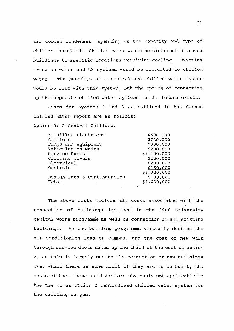
72
air cooled condenser depending on the capacity and type of
chiller installed. Chilled water would be distributed around
buildings to specific locations requiring cooling. Existing
artesian water and DX systems would be converted to chilled
water. The benefits of a centralised chilled water system
would be lost with this system, but the option of connecting
up the seperate chilled water systems in the future exists.
Costs for systems 2 and 3 as outlined in the Campus
Chilled Water report are as follows;
option 2; 2 Central Chillers.
2 Chiller Plant rooms Chillers Pumps and equipment Reticulation Mains service Ducts Cooliing Towers Electrical Controls
Design Fees & contingencies Total
$500,000 $720,000 $300,000 $200,000
$1,100,000 $150,000 $200,000 $150,000
$3,320,000 $680,000
$4,000,000
The above costs include all costs associated with the
connection of buildings included in the 1986 University
capital works programme as well as connection of all existing
buildings. As the building programme virtually doubled the
air conditioning load on campus, and the cost of new walk
through service ducts makes up one third of the cost of option
2, as this is largely due to the connection of new buildings
over which there is some doubt if they are to be built, the ~
costs of the scheme as listed are obviously not applicable to
the use of an option 2 centralised chilled water system for
the existing campus.

73
A revision of the above costs to derive a rough order of
costs for a central chilled water system for the campus is
based on the following assumptions;
1. Only large loads in close proximity to the central
chiller plant should be connected to the system. The costs
of connecting a small chiller in a remote building will far
outweigh any possible savings, especially when the electrical
loading of a compression air conditioner is only about 30 to
40% of its chilling or rated capacity as it has a COP of about
2.5 to 3. By applying this criteria to the systems,
uneconomic conections will be avoided and the benefits of
centralised chilled water systems applied to plant which will
show the maximum savings.
2. with the reduction in chiller capacity due to the
building programme not proceeding the construction of new
underground chiller plantrooms and new underground ducts can
probably be avoided by incorporating the new chiller plant in
existing service spaces.
Rough order of Cost of two central chilled water systems
based at Engineering/science lecture theatres and Arts lecture
theatres.
Chiller Plantrooms alterations Chillers Pumps and Equipment Reticulation Mains Cooling Towers Electrical Controls
Design Fees & contingencies Total
OPTION 3
$50,000 $410,000 $200,000 $100,000
$90,000 $200,000 $150,000
$1,200,000 $245,000
$1,450,000

74
From the MOWD report the conversion of all the existing
artesian. water, and Direct Expansion plant to individual
chilled water operation was estimated to cost $850,000.
All the above figures are based on 1987 equipment and
construction costs.
Operating costs
Electrical consumption and maintenance charges are the
main operating costs associated with air conditioning plant.
While both costs should be significantly lower for the central
chiller plant system (option 2) than for the individual
chiller installations (option 3), the actual costs are
difficult to assess without reasonably accurate air
conditioning demand data. The MOWD report estimated a saving
in operating costs of $11000 annually for the central chiller
plants, when compared to the individual installations, however
this was for the case of satisfying the additional load due
to the building expansion programme. Very little is known
about the actual operation of air conditioning plant on
campus, and even rough estimates of costs are difficult to
make.
For any centralised air conditioning plant for this
campus the capital costs are massive and are unlikely to be
recovered by any possible energy savings. The low cooling
load density and the fact that the cooling demand exists only
for short intermittent periods in summer are the main reasons
for the limited economic viability of any centralised scheme.
2.3.3. EVAPORATIVE COOLING.
Evaporative cooling is an energy efficient, cost

75
effective method of cooling suitable for comfort air
conditioning in institutional buildings in dry hot climates.
In investigating the suitability of the Christchurch climate
for evaporative cooling a weather data file was used to
determine the actual extremes in dry bulb and wet bulb
temperatures. The file (Climdata 69 generated by the NZ
Meteorological Service) contained hourly dry bulb and relative
humidity data for the year 1969. coincident dry bulb and wet
bulb data were derived from this and analysed to determine the
extremes limiting an evaporative coolers performance.
Evaporative cooling Of Air.
1. Direct Evaporative cooling.
Evaporative coolers, air washers, sprayed cooling coils,
or humidifiers are used to cool air directly by evaporating
water directly in the incoming air stream. The dry bulb
temperature is lowered as the air condi tion moves
adiabatically up the wet bulb line corresponding to the air's
wet bulb temperature. As the moisture content increases with
direct evaporative cooling the resulting conditioned air has
a higher humidity.
2. Indirect Evaporative Cooling.
A secondary air stream is cooled by direct evaporative
cooling, this sensibly cools the fresh air stream to the
conditioned space through a heat exchanger. Figure 2.4
shows the two processes on a psychrometric diagram.

76
Because the final dry bulb temperature is determined by the
wet bulb temperature of the incoming fresh air, the
performance of an evaporative cooler is directly related to
the climatic conditions. Evaporative cooling is therefore
best suited to dry cool climates with low wet bulb
temperatures.
Basic weather data for the Christchurch area suggest
evaporative cooling of air for air conditioning may be quite
successful:
1% std. Dev.DB Temperature 27.8 Mean Coincident WB Temperature 2% std. Dev.DB Temperature Mean Coincident WB Temperature
deg C 17.8 deg C 26.0 deg C 17.2 deg C
[Watt 1986]
Figure 2.5 shows the ASHRAE comfort standard 55-74 plotted on
a psychrometric chart, with the above maximum DB, and
coincident WB temperatures plotted. Also a typical summer
peak hot day (Jan 19 1969 fro~ Climate data file) hourly
temperature profile is plotted. It can be seen that even
allowing for less than ideal cooler performance, direct
evaporative cooling should be capable of achieving the
necessary comfort conditions on this worst case day.
The actual size and type of evaporative coolers used will
depend on the total load of the air conditioned space, and the
use of that space. The libraries for instance may require
closer control of humidity than that available from an
evaporative cooler, and require the use of indirect
evaporative cooling.

i) -4?.!:,cJ'
€l;qpo 'PvJ2'-lve
COO-l-l4'Q
SIMPLE INDIRECT ~ EVAPORATIVE COOLING"""iIIr---------'o OUTSIDE AIR
.. 0 MIXED RETURN/OUTSIDE AIR REFRIGERATED
AIR CONDITIONING
FIGURE 2.4 DIRECT & INDIRECT EVAPORATIVE COOLING -.J -.J

78
Evaporative Cooling Of chilled Water.
The existing artesian water supply to cooling coils on
campus is at a temperature of about 12 deg C. The possibility
of achieving this temperature for air conditioning chilled
water by evaporative cooling is addressed in this section.
The evaporative cooling of a liquid is both a heat and mass
transfer process occurring on the free surface of the liquid
by the combined effects of:
a)heat transfer by conduction
b)heat transfer by radiation
c)surface evaporation of the liquid
Cooling water is recirculated through an air flow/cooled by
evaporation, while the enthalpy of the air increases as it
becomes more humid.
Make up water for evaporative losses is of the order of
1 percent of the circulation rate [Jones 1989]
As with evaporative cooling of'air the wet bulb temperature,
and particularly its depression below dry bulb temperature
determine the applicability of evaporative cooling.
At night, wet bulb temperatures are lower than during the
day, (see Figure 2.5) and evaporative cooling efficiencies are
improved. In a climate where evaporative cooling is
unsuitable for use during the day the application of chilled
water storage combined with evaporative cooling of the chilled
water to charge up the storage volume at night can make
evaporative cooling attractive. An added benefit is that,the
cooling plant is run on night rate electricity.

10
XA
Xi}
o
~k
~,
C"
1% SD COINCIDENT I'IB. DB. \'t-Q,
,<-' 60 -- • ' -- 'I ~ -·ce A$*¥!~
2% SD COINCID2:l'iT lIB. DB.
ASllI\AE comfort standard «--1.. standard 55-74 0'?''v • -.'.'.'. y /,<:(:.=
~'" SQ Hourly temperature <c" , . """~9..v~.
~ s : /,~-=-<G. ~"v. ,;r;
Outside Air
<1Q
J~ ~
~~..;:
" ",f"'~' ':-~'t-"
.. _ ~ ,..-::;:-:: .~'0~ • " " _ __ c,.,'?'
p
'~'~
- -. S:::;:.'
" ,~/'---'-7"~ "1, ,.
~
.z ~
70 ;
~~,L \/ 0\0 , o\o_~_o\,,-:
, C) C).+--+-~C) -Q) ~ ->r-+- '\
-.'. or' =-«)C)_t?' •
*~~==!5: I __ ':;~ c':t: i;
I~;
~
~1:5----2
.",-<::-
-c-7S~
~==sJ~ "YLb~_ --,J\~ 0 --,---,~ o =J;;<~~',§J:S;~'l-iL,--~
10 15 20 25 30 o 5 DRY BULB TEMPERATURE- DC
-........ --...." --..... '--"'" ---...." '--""" --...." --...." -........ --...." --...." --..... --...." -----.. ~--...." --..... ------ -..;::.", --"""'-"""" o 10 ?~O ENTHALPY kJ/kg
',-<-)0'
--'''' ~/,--'
c::;-
~
010 t>'?-..!-
aC,O "
0~
:?o~
17 =:i=s:1 f- , ....
16 z w' ....
15 fz
148
13 W a:
_I? ::J , .... -f-
U)
; 11 0 _l~ I 2:
~iJO -.,.-/9 , . ;~-
8
-'7
100
90
80
70
~13 .... 60
.---=-12
::.......-
"KrO-'=:-s -. '3- '>.;.. I ,. '0:--= '" . 1 l' '-' -
(J'. :'
35 40 ,0
--...." --..... --....,,--.....-........' .... -........ --...." 50
30
FIGURE 2.5 h~APORATIVE COOLING TEMPERATURE CONSTRAINTS
-."j
1.0

80
"Larger central cooling plants such as college campuses or other district cooling plants, represent another potential application. occasionally central plants can take advantage of existing equipment in the process of retrofitting. A plant change from absorption chilling to compression chilling, for example, would make available a significantly oversized cooling tower that could work quite well as an evaporative chilling tower in conjunction with thermal energy storage capability." [ Hat ten M.J.1989]
The maj ori ty of air conditioning plant on campus is sized
to operate on 12 deg.C artesian water, a temperature
attainable by evaporative chilling for the majority of the
year.
There will be periods during summer when the evaporative
coolers will need to be supplemented by conventional chillers.
with the use of thermal storage, night operation of the
chillers, will minimise the costs of extra chilling capacity.
As supplimentary cooling is required in summer only there
should be no increase in electrical demand peak charges.
Figure 2.6 shows a schematic diagram of an evaporative chiller
with thermal storage system which allows topping up or backup
with a conventional chiller.
There are several methods of achieving evaporative
cooling of chilled water.
a) Cooling Tower. The open water cycle used here requires
the use of heat exchanger between the cooling tower and the
chilled water system. .. b)Closed Circuit Evaporative Water Cooler. The closed
water circuit used here removes the need for the external heat
exchanger used for the cooling tower. Sludging, chemical
dosing, and microbial problems are reduced significantly.
c) Strainer Cycle. This is a patented system allowing

REFRIGERATION EVAPORATOR
CHILLED WATER STORAGE TANKS
I CONDENSER
COOLING TOWER
REFRIGERATION CONDENSER
;;;---------a..-.- CHILLED WATER F
1-......-----------------;l1li-- CHILLED WATER R
FIGURE 2.6
EVAPORATIVE CHILLING WITH THERMAL STORAGE

82
direct use of a chillers cooling tower to provide direct
evaporative cooling of chilled water. capacity is however
limited as the cooling tower will be sized for a greater water
temperature difference due to the higher condensor
temperature.
"Chilled water storage and eutectic salt storage are applicable for direct evaporative chilling. In genera 1, ice will not work as a thermal storage medium for e vaporative chilling because the working fluid temperat ures are lower than what is practical to achieve with a cooling tower."
[Hatten M.J.& Johnston T.W.]
Because of the need for chemical dosing of cooling tower
water to restrict microbial growth, indirect evaporative
cooling using heat exchangers or operating the chiller as a
heat exchanger is the preferred method of evaporative
chilling.
Evaporative Cooling And Legionaires Disease.
Bacterial growth in 6pen water systems in air
conditioning systems is a significant problem, causing
fouling, corrosion, and health hazards. It can be controlled
by chemical dosing and careful maintenance, but these are
understandably disliked. The extent of bacterial growth
is determined by several factors. M. H. Lyons discusses the
conditions required for bacterial growthi
"The occurance of the main Legionaires Disease bacterium, legionela pneumophila, is common in nature but appears to be rare in properly treated cooling water systems. It has fairly specific requirements if we try to grow it in the laboratory and these are, a source of dissolved iron, a source of the aminoacid cystine, a pH between 6.6 and 7.2, and a temperature of between 20 and 50 deg. C."

83
As the water operating temperature in an evaporative
cooler is not significantly above the wet bulb temperature of
the air (which in Christchurch is at the lower limit of the
bacterial growth temperature range) the chance of bacterial
growth wili be severly limited. Watt 1986 states that there
are no reported incidents of Legionaires disease associated
with evaporative coolers.
2.3.4 DISCUSSION - CAMPUS COOLING.
While operating cost savings are possible with
centralised chiller plant, the installation costs are
considerable, and without detailed data on the operating
characteristics of air conditioning plant on campus a more
accurate economic analysis is not possible.
The use of evaporative cooling on campus appears to be
quite feasible. Combined with careful energy efficient
design of new buildings it would be capable of providing cheap
energy efficient cooling for buildings on the campus.
Similarly the use of evaporative chilling of cooling
water in conjunction with a moderatly sized refrigeration
cycle water chiller appears to be technically feasible and
considerably cheaper than a conventional centralised or local
water chiller installation.
In any case the operating costs will be higher than those
with the current situation where the majority of cooling is
derived by free cooling with artesian water.

2.4 THERMAL STORAGE SYSTEMS.
2.4.1 THERMAL STORAGE BENEFITS.
84
In order to maximise the use of cheaper off-peak
electricity rates, thermal storage can provide the means of
bridging the time lag between energy consumption when it is
available cheaply, and the desired end use of that power,
typically during daytime demand peaks.
The most obvious example of thermal storage in use is the
common domestic hot water cylinder, which is invariably on a
separately metered ripple controlled electricity supply, at
a lower charge. Depending on the particular features of a
thermal energy user, there are many thermal energy storage
alternatives available.
2.4.2. Cooling Thermal Storage.
In light of the university's probable need for an energy
efficient chilled water supply, analysis of the potential
benefits of low temperature storage for the campus is
important.
The main benefits of cool thermal storage are;
1. Thermal storage and load shifting can provide on peak
cooling (or heating) at close to off peak costs. This
advantage only applies to systems where the air conditioning
load is coincident with the electrical demand peak charges.
As electrical demand peak charges occur during winter in New
Zealand, the argument for thermal cold storage in order to
reduce peak electrical demand charges is contradicted.
[STEWART L.J.]
However air conditioning loads with a low solar

85
component may still have a significant duty during winter
electrical demand peak periods, and thus benefit from cold
thermal storage.
2. Reduced investment in refrigeration equipment as plant
can be sized to average demand rather than peak demand.
3. An appreciable reduction in power cost can be achieved
due to;
a.Increased operating efficiency of chilling plant as
it runs at optimal design capacity continuously
b.Higher refrigeration COP of chillers run at night
when ambient temperatures are lower.
c.The reduction in peak capacity, combined with the
effect of shifting chilling load to off peak electricity
periods, considerably reduces electrical demand charges,as
well as the reduction in electrical energy consumption.
4. Because of the ability to shift the time of operation
of the chilling plant the potential for operating the storage
system as a heat pump providing useful heat for buildings
exists.
The ability to use the reject heat off the chilling
system is dependant on finding a suitable heat sink. with
night rate electricity powered storage chillers the
possibility of using the reject heat for pre-heating buildings
for the following day is the most obvious solution.
Two main thermal storage systems exist, chilled water and
ice storage.

'86
2.4.3. Chilled water storage Systems.
Of the common materials available for thermal storage
water has the highest specific heat capacity (4.18 kJjkgK).
As water is widely used as a heat transfer medium in building
services it is a prime choice for use in thermal storage
applications.
Chilled water for air conditioning normally has a flow
temperature of about 6 deg C, therefore chilled water storage
is required at or below this temperature. Return water from
the air conditioner is at about 15 deg C. In order for the
chilled water storage tank to be capable of storing any
thermal capacity (or thermal energy it must operate across
a temperature differance equal to or greater than the
differance between chilled water flow and return temperatures.
Ideally two storage tanks are required, one to store chilled
water and one to store the warmer return water. Chilled water
is then stored by circulating warm returned water through a
chiller to the cold tank, and the chilled water storage is
used by circulating the chilled water from the cold tank
through the air conditioning plant. without separation of the
cold and warm parts of the thermal store, blending of the cold
and warm water reduces the temperature differance to zero, and
with no temperature differential no energy storage is
possible.
"This leads us to the conclusion that the effectiveness of a chilled water storage system is directly dependant on the amount of temperature differential between the tanks. It would be best if we could devise a way to accomplish this with a single tank." [Trane Co 1976]

87
Several systems for maintaining the temperature
differance in a water storage system are in usei
I.Temperature stratification in a Single Tank.
Return water at 15 deg C can float above stored chilled
water at 5 deg C due to its lower density. A thermocline/or
zone with a steep temperature gradient, is present between the
lighter warm water on top and the denser cold water below.
The effectiveness of the stratification (and hence the
resulting thermal storage effectiveness) is dependant on
reducing turbulence within the tank, especially at the inlet
and outlets, resulting in the use of large diffusers at these
points. Also the tank shape is limited to narrow vertical
tanks of constant cross-section. As the thermocline may
increase to a depth of 2 meters this system is only really
suitable for a tank of considerable vertical height.
2. Flexible Diaphragm in a single tank.
Here a flexible diaphragm takes the place of the
thermocline. The only losses are leakage and the thermal
conductivity through the diaphragm, as blending between the
stratified regions is prevented by the diaphragm. In
operation the diaphragms can split and wear, althQugh small
holes have a negligible effect on the system performance.
3. Multiple Tank Systems.
By storing the water in separate tanks a maximum
temperature differential can be achieved.
double the total storage volume required.
However this would
By compartmenting
a large tank, or installing a large number of small tanks and
circulating between individual tanks this can be avoided.

88
"If the number of compartments in a tank is assumed to be n, then the number of compartments filled with water is n-1: one compartment is empty ....... The storage efficiency of such an arrangement depends on the number of compartments in each tank and is given by the formula;
(n-1)/n x 100% E Thus if the tank is divided into six compartments the efficiency is;
(6-1)/6 x 100% = 83.3%" [Linton KJ]
Figure 2.7 shows a typical multiple tank chilled water
storage system
The value for efficiency given here describes the ratio
of useful thermal storage capacity to the total tank volume.
constructing a labyrinth of interconected compartments
can achieve a reliable temperature differential between the
inlet and outlet of the storage system with negligible mixing.
The main disadvantage of water based storage systems is
the cost of the large storage tanks. If a suitable site can
be found chilled water storage can be attractive especially
as existing chiller plant can be directly connected to the
storage system

..-II "'11" 15°C R
~!~
~ ~
~
ISoC ISoC soc soc 15°C SoC
I------~~~~~ .! Z
t><ll!><l l> ...-- ~"'SOCF
CHILLER
FIGURE 2. 7 ~1ULTIPLE TANK CHILLED WATER STORAGE SYSTEM
co \.0

90
2.4.4. Ice storage systems.
In an ice storage system the ice is used for low
temperature energy storage only, water chilled by the melting
ice in the storage tank is used to transfer the stored cold
energy to the air conditioning plant. By utilising the high
latent heat of fusion (freezing) of water (335 kJjkg) the
volume required for storage is reduced considerably. For a
given volume an ice store can store about ten times the energy
of a chilled water store. As well as this the release of the
thermal energy of the latent heat of melting ice occurs at the
constant temperature of 0 deg C, allowing the problems of
increasing chilled water flow temperature to be ignored.
In a new installation (where existing chillers are not
available for connection to a chilled water storage system)
ice storage is generally cheaper.
"A lot of refrigeration can be purchased for the differance in storage tank costs. Ice storage tanks take up much less storage space volume - only about one tenth of the volume in this example. The storage system is less expensive and weighs a lot less. Essentially all cooling (energy) can be extracted from storage.- with ice, problems of stratification, seperation, or sucking a tank dry etc are all avoided." [stamm RH]
Ice storage system refrigeration plant suffers from a
higher energy consumption for a given capacity when compared
to chilled water. The increased energy consumption is due to
the lower COP resulting from the lower evaporator temperature
required to produce ice.
There are three main types of ice storage systems;
1. Ice on Coil - External Melt System.
Ice is built up on banks of serpentine coils submerged
in an insulated tank of water. The refrigeration system
91
builds up ice on the outside surface of the coils by
circulating either, cold ethylene glycol brine through the
coils, or by directly feeding low pressure refrigerant into
the coil. When the ice has reached a designated thickness the
refrigeration system is shut down. When chilled water is
required the ice on the coils is melted by direct contact with
the warm return water from the air conditioning plant. During
this cycle the tank water is agitated by air bubbles from a
low pressure distribution system beneath the coil in order to
improve heat transfer. [Baltimore Air Coil]
Figure 2.8 shows a typical ice on coil system.
2. Ice on Coil - Internal Melt Systems.
This is similar to the ice on coil system described
above. A glycol brine solution circulates throughout the
entire cooling loop (from refrigeration chiller, through
storage, to air conditioning plant load)and builds up, and
mel ts the ice from the inside of the pipe on which it is
built.
"With this arrangement, the first ice to melt is that which is in immediate contact with the coil tubes. As the melt-out process continues, an annulus or ring of water develops between the tube and the ice, which continues to grow in thickness as the ice melts. The annulus provides an increasing resistance to the transfer of heat from the ethylene glycol to the ice, since the thermal conductivity of water is one - fourth that of ice. As a result of this design approach to internal melt, the ethylene glycol temperature rises with time.
[ Mc Cullough JM 1988 ]
A variation of this system uses an 11 ice lens" system
which attempts to overcome the heat transfer limitations by
packing a large number of small water filled plastic

92
containers into the storage tank.
3. Ice Harvester systems.
The ice making surface is typically suspended above the
ice storage tank. The ice making surface consists of
evaporator plates over which water flows.
sides of the plates in sheets about
Ice forms on both
6mm thick. At
predetermined intervals hot refrigerant enters the plates
causing the ice to break away and drop into the tank. The
cycle is repeated as long as there is need for additional
cooling reserves.
The advantages are that the ice harvester system gives
a large heat transfer area to the circulating chilled water,
allowing rapid melting with no risk of short circuiting of the
return chilled water. This allows a continuous ice making
capability which is impossible with systems where the coils
are submerged in the ice storage tank, as the coil becomes
encased in ice, insulating the heat transfer surface and
reducing the efficiency of the system.
Figure 2.8 shows the operation of a typical ice harvester.

CHILLED WATER
CHILLED WATER
EVAPORATOR COIL
AIR DISTRIBUTER
ICE ON COIL SYSTEM (EXTERNAL MELT)
PLATE ICE MAKER
ICE/WATER MIXTURE
ICE HARVESTER SYSTEM
FIGURE 2.8 ICE STORAGE SYSTEMS
GLYCO OR
D.X. HILLE
93
RECIRC. PUMP

94
Ice store System Configurations.
1.Full Storage.
The ice store is sized to provide the total daily cooling
for the design cooling load. As the design load is based on
the worst conditions, ie maximum building occupancy on the
warmest expected day, the system will be severely under
utilised for most of the year. Capital cost will be high, as
in effect the system will be oversized by a factor of two, as
the chiller or ice store alone will be capable of serving the
design cooling load individually.
2.Partial storage.
Both the chiller and store are run during the day to
satisfy the cooling load, with the chiller charging the store
at night. This results in an approximate reduction in chiller
and ice store size of 50%.
Electrical energy consumption is reduced by a similar
factor, and by operating the store only during demand peak and
high energy cost periods, the chiller day operating costs will
be held at a low level
This is a particularly suitable option for the university
which faces its demand peak charges in the three winter
months, when its cooling requirements are quite low.
Chiller/store Arrangement.
wi th a full storage system the chilled water distribution ~-~--..
system interfaces with the ice store only, however with a
partial storage system both the chiller and ice store provide
cooling, individually as well as simultaneously.

Three chiller/ice store arrangements exist;
1. store Led Series Arrangement.
95
Refer to Figure 2. 9a. Here the chiller has the highest
possible suction temperature, and therefore the highest COP.
Although the ice store gives off its cooling energy at
constant temperature of 0 deg C, it faces a lower temperature
restricting its melting capacity.
The store is charged by switching the three way valve to full
bypass, (isolating the load from the store)
Full load operation has the three way valve on full flow
with maximum chilled water temperature difference across the
chiller and ice store. Part load operation has the valve
modulating to provide a constant chilled water flow
temperature. If constant flow temperature is not important eg
if dehumidification is not neccessary, the control valve may
be located in the chilled water return line maximising the
return chilled water temperature to the chiller.
2.Chiller Led Series Arrangement.
Refer Figure 2. 9b. with the chilled water already cooled
by the ice store the chiller has a lower COP, than if in a
store led configuration.
The ice store has improved cooling performance. Because of
this, this system lends itself best to loads requiring a boost
in cooling for only a short period. As the store is drawn down
rapidly it may be quite small.
3.Parallel Arrangement.
Refer to Figure 2.9c. with the chiller and ice store in
parrallel, output of each is controlled by individual valves.

ICE STORE
CHILLER EVAPORATOR 1----'------ 15 °C R
FIGURE 2.9a STORE LED SERIES ARRANGEHENT
CHILLER EVAPORATOR
ICE STORE
1---1"l!t<:::1~--....l------15°C R
FIGURE 2.9b CHILLER LED SERIES ARRANGEMENT
J-L----I--------=------- 15°C R
FIGURE 2. 9c PARALLEL ARRANGEHENT
FIGURE 2.9 CHILLER - ICE STORE ARRANGEMENTS
96

97
Both the chiller and ice store face the same chilled water
return temperatures maximising performance of each item.
Under full load operation both the chiller and store provide
maximum output. At part load the chiller operates at full
output, with any excess of demand over the chiller output
being passed to the store.
Ice store operation.
Refer to Figure 2.10.
1.Store Priority.
The ice store operates as the cooling base load while the
chiller makes up any extra required capacity. The chiller
operates at reduced capacity, resulting in a lower cOP. The
peak demand consumption of the chiller is indefinite but will
be minimised. There is a tendency for both the chiller and
ice store to be oversized with store priority, resulting in
increased capital costs when compared with chiller priority.
store priority works best with a time of use electrical tariff
as the chiller can be shut down during high electrical cost
periods.
2.Chiller Priority.
Here preference is given to running the chiller at full
load, which is sized to provide a daily base load as well as
the night ice store charging duty. The ice stores output
modulates to provide the peak cooling load. Ice store charging
operation of the chiller is minimised, which is desirable as
ice making incurs a loss of COP.
Where there is a peak demand function to the electrical tarrif
this system is ideal as there little to be gained from

~ H
~I--------' u
~ NIGHT H STORE 8 CHARGING u
o 7
/ /' PEAK
//// CHILLER // COOLING
STORE COOLING
NIGHT STORE CHARGING
23 HOURS
FIGURE 2.10 STORE PRIORITY OPERATION
~ H
~J..------l U
~ NIGHT H STORE 8 CHARGING u
PEAK STORE NIGHT
. ...L. _____ CO_O_L_I_NG __ ""'--.I STORE CHARGING
o 7 23 HOURS
FIGURE 2.10b CHILLER PRIORITY OPERATION
FIGURE 2.10 PARTIAL ICE STORAGE OPERATION
98

99 using the chiller at less than full output at times when
demand isn't at peak levels. This is especially
applicable to the university's case where demand peaks are
moni tored for three months in winter, where providing the
control system allowed the ice store to meet the total cooling
load during winter demand peaks, and shut off the chiller in
winter, the chiller priority system would be most applicable
for operation for the rest of the year.
Ice storage System sizing And Selection.
In order to achieve any of the benefits of an ice storage
system both chiller and ice store size must be optimised for
the cooling loads and frequency of those loads, the type of
store and chiller configuration, the electrical tariff
structure, and the control strategy.
2.4.5. Ice store Operating strategy For The Campus
Sizing and Selection.
100
1. Size the chiller and ice store for chiller priority
operation based on air conditioning cooling load design
conditions in March. This will achieve;
a) Peak cooling loads will be satisfied by the chiller
and ice store operating together in chiller priority, when
normal term occupancy is coincident with the hotest weather
conditions.
b) During periods when the cooling load is reduced ego
spring/autumn when a significant part of the cooling load is
achieved by free cooling, operation on either store or chiller
alone to make up any extra load depending on energy costs at
that time.
c) During winter energy demand charge periods the ice
store alone should cope with any balance of cooling loads over
that satisfied by free cooling.
The chiller priority sizing will ensure minimum capital
cost of chiller and ice store.
The above design assumes that maximum benefit of free cooling
is achieved by fresh air / recirculated air control by both
temperature and enthalpy control. All spaces shoUld be pre
cooled before occupancy.
When simple control is used on the storage system the
system can only be optimised for one load pattern/energy
tarriff structure. However the campus has an EMCS capable of
making dynamic plant operating decisions based on immediate
cooling load and energy tarriff conditions. For this reason

101
parrallel conection of the chiller and store, will best allow
optimum chiller COP and ice store meltout to be attained
regardless of the EMCS selected method of operation.
operation.
a) Summer.
During summer vacations any lecture theatres in use will
be booked on the EMCS so the EMCS can determine the required
level of ice to be built up enabling store only operation
without excessive ice building,or day chiller operation. The
decision on whether to make ice and use the store on the next
day or run the chiller during the day depends on the ratio of
chiller day COP to night cop and energy costs.
ie if cop night ice making < ($/kWh d / $/kWh n)*COP day
then it will be cheaper to run the chiller on chiller priority
during the day
Currently the summer night/day energy cost is 3.38/4.61
or 0.73. So if the chiller cOP at night is lower than 0.73 of
the chiller day cop then the system should be run on the
chiller during the day.
During summer term time eg March, the system will run on
chiller priority, but may run on store depending on the
pricing differential between summer day and night rate energy
costs.
b) Spring/Autumn.
Where possible cooling will be achieved by free cooling
using incoming fresh air. Any balance required can be made
up by the storage system running on chiller priority
or store priority depending on thenight/day energy pricing

differential.
c) winter.
102
As for spring Autumn operation free cooling should make
up most of the cooling load.Any balance will be made up by the
storage system running on chiller or store depending on the
night/day energy pricing differential.
However during the months of June to August the system will
operate on store only during periods when the EMCS determines
demand peak charges are likely to be incurred. The winter
pricing differential may be such that the store only will be
run during the day. It is likely that the store alone will
satisfy winter cooling loads.
2.4.6. Alternative Systems.
Binary Fluids.
A binary fluid is a mixture of fresh water and another
fluid, typically ethylene glycol. When the solution is
chilled the fresh water is frozen out of solution, forming
discrete ice crystals, resulting in a binary fluid slurry
which is pumped to storage, where a porous ice pack forms.
Because of the high surface area of the ice crystal pack the
binary fluid storage system can discharge its stored energy
rapidly similarly to the plate ice harvester.

103
2.4.7. HEATING THERMAL STORAGE.
As virtually all of the energy used for heating on campus
(both space heating and domestic hot water supply) is derived
from the steam district heating system the scope for
improvements by using heating thermal storage is limited.
Because the steam is produced from coal fired boilers which
are in operation all year round there is little need for
storage, as the coal can be burnt at any time with no loss of
thermal efficiency or cost penalty.
However this situation would be quite differant if an
alternate strategy for boiler operation was introduced. If
the boilers and steam district heating system were in
operation only during the winter heating season, the
requirement for domestic hot water would be best satisfied by
night rate electric water heating storage tanks. There is
also some question as to the ability of the existing boiler
plant to meet expected growth in steam demand with expansion
of the campus buildings. Thermal storage can play a role
here in offsetting peak building steam demands, and prevent
the need for increased boiler capacity.
Phase change material s (PCMs) and Eutectics use the
latent heat of phase change of various materials for thermal
storage at a wide range of temperatures. However these are
used only in a limited number of systems overseas and unlikely
to be commercially acceptable in New Zealand.
2.4.8. DISCUSSION - THERMAL STORAGE SYSTEMS.
with a cost of over $500,000 for an ice storage system
capable of supplying cooling for about half the campus, and
104
a similar cost for chilled water storage, assuming sUfficient
space can be found, either of the cooling storage systems
are likely to be economically untenable. As with the district
cooling schemes the high capital cost is unlikely to be
recovered in savings. conventional chillers would have lower
capital costs and while still using energy at peak day time
periods, may still be cheaper to operate in the long term if
maintenance for the storage systems proves expensive.
The ability of evaporative cooling to provide
inexpensive energy efficient air conditioning for the campus
deserves further consideration as it avoids the high capital
costs of the al ternati ve schemes, and has low operating costs.
In some cases evaporative coolers may be easily installed in
existing air conditioning and ventilation plants.
105
2.5 CONVERSION OF STEAM TO HOT WATER HEATING.
2.5.1 STEAM TO HOT WATER CONVERSIONS.
operating cost reductions of the order of an estimated
20% (actual saving 40%) are reported by Yetman, for the
conversion from steam to hot water heating. Similarly Cole
1989 describes hot water conversion of three west coast
hospitals where energy usage reductions ranging from 27% to
45% were achieved. The motives for conversion were;
1. Boiler age and condition
2. Difficulty in finding certified boiler attendants
3. Energy cost savings
4. Salary reductions through elimination of the
requirement for full time boiler attendants
As well Yetman claims reductions of 40 and 50% in capital
cost for hot water boilers compared to steam boilers. For
the university to replace its existing steam boilers it would
face a cost of $M2.6 for steam boilers, (source Fig 5.1 The
Potential For Cogeneration Of Heat and Electricity ) or about
$M1.3 for hot water boilers, using Yetman I s claim of 50% cost
of steam boilers for hot water boilers.
Improvements in thermal efficiency of boiler plant are
due to many factors, and while the physical design of shell
boilers (whether steam or hot water) has not altered
significantly, modern boiler control systems and operational
methods have improved boiler efficiencies.
The main advantages of hot water over steam heating are:
1) Thermal Inertia. A large volume of water is
constantly circulated around the heating system mains, and

106
this acts as a thermal flywheel damping out fluctuations in
demand. At present the campus steam boilers have problems
following the demand for steam as it varies throughout the
day. The existing shell boilers contain a large volume of
water and have chain grate stokers, resulting in a high
thermal inertia boiler system. Altering boiler output
significantly takes about 30 minutes especially if there is
a deep bed of coal burning on the stokers. As steam loads are
shut off or started up on campus the steam pressure fluctuates
faster than the boilers can keep up with, occasionally blowing
safety valves.
2) Lower System Heat Loss. The closed hot water system
eliminates the losses associated with leaking steam traps,
valve and pump glands, boiler blow down, and open condensate
receiver flash loss and hot well losses.
3) Reduced Maintenance. Elimination of steam traps,
condensate return systems, pressure control valves, safety
valves, etc significantly reduces heating system maintenance
requirements.
4) Improved Control. steam system control is complicated
by the fluctuation in steam pressure as well as flow rate as
loads vary. For hot water systems the return temperature only
varies, as the hot water system operates with constant flow
rate and output temperature.
5) Economics. Higher system efficiencies are claimed for
hot water systems, as well as reduced operating costs, main-
tenance and downtime.

107
Pressure and Temperature Constraints
In order to achieve flow temperatures above say 85 degC
without boiling the hot water system must be pressurised.
The flow temperature limit is determined by the saturation
pressure of the system with a flash margin added as a factor
of safety. For the campus system pressurisation could be
achieved by either a static head due to a system feed tank
located on the roof top of say the Physics building, or by
using a gas pressurised expansion vessel. The system feed
tank is simplest and would give a system upper temperature of
about 120 degC. This is based on a building height of 30m
giving a static head of 3 Bar with corresponding saturation
temperature of 133degC, and subtracting a 15deg flash margin,
to give a system upper limit of 118degC. As the amount of
energy transmitted is a function of the flow and return
temperature difference, a_return temperature at least 20 deg
below the flow temperature is desirable.
Another approach is to match the hot water flow
temperature to the saturation temperature of the existing
steam system ie 165degC ( from sat.steam @ 7 bar). Existing
heat exchangers and calorifiers would not be derated
significantly if this was done. The system would have to be
pressurised by a pressurised expansion vessel.
steam / Hot Water Operating differences
A simple analysis of both the existing steam heating and
hot water systems gives the following results:
I} System Efficiency. currently the steam heating system
is operating at an estimated efficiency of 65% [source, main-

108 -
tenance department staff] during the winter heating season.
At other times of the year as the heating load reduces, while
circulation and operational losses remain constant, the
efficiency drops even further.
2) System Leakage. 95% of condensate (at 75degC) is
returned to the boiler hot well with the existing steam
system. Also [Beal 1987] gives a steam system leakage rate
of 5.0% and hot water system leakage rate of 0.5%. The hot
water system circulates approximately 10 times the mass of
water of the steam system so the volume lost is about the
same, however the steam enthalpy is greater than the hot water
enthalpy.
3) Boiler Blowdown. The quantity of boiler water lost
during blowdown is difficult to determine as blowdown is
intermittent, with no heat or flash recovery used. Blowdown
rate, whether continous or intermittent, is determined by the
percentage of dissolved solids in the boiler, so for a given
boiler installation the blowdown rate should theoretically be
the same whether continous or intermittent blowdown is used.
Beal gives a continuous blow down rate of 2% of steam flow for
a boiler installation with 95% condensate return.
4) Feed and Circulation Pumps. As the campus steam
system uses Weir steam driven boiler feed pumps, and there are
no extra pumping costs associated with the steam system, the
pumping energy requirements are part of the boilers net energy
consumption. The hot water system will require electric
boiler feed pumps and system circulating pumps for each
heating main. Main circulating pumps are estimated to have

109
the following duties;
HEATING FLOW HEAD PUMP MAINS RATE LOSS MOTOR
Engineering 11kg/s 95kPa 2.5kW Science 23kg/s 93kPa 4 kW Arts 38kg/s 310kPa 18 kW
Appendix E contains analysis of the operation of both
steam and hot water heating based on a design heating load
derived from the present campus annual heating energy
consumption. The results given below are largely comparative
as the annual mean design load doesn't take into account the
effect of varying heat loads and plant efficiencies during the
year on the two systems.
2.5.2 STEAM/HOT WATER HEATING ANALYSIS RESULTS.
Annual Operating Costs for Steam System. Fuel 4390 tonnes @ $88/tonne. Water treatment $5000/ann. Boiler operators 5 * $80,000 Steam system maintenance
assume 2.5 Fitters @ $30,000 * 2
Note.
$386,320 $5,000 $400,000
_~l;;n 000 ~941,320
As exhaust from the Weir boiler feed pumps is used for heating the hot well, and the Weir pump exhaust losses are fel t to be recovered by the improved boiler feed· water condition they are neglected.
Boiler operator salaries are taken at the true cost to the university, that is twice the gross salary paid. Annual Operating Costs for Hot Water System.
Fuel 3862 tonnes @ $88/tonne. Water treatment - negligible Boiler operators 1 * $80,000 Pumping operating costs Steam system maintenance
assume 0.5 Fitters @ $30,000 * 2
$339,912
$80,000 $4220
$30, 000 $45Lf ,132
with the hot water system, coal consumption is reduced
to 87% of that required by the present steam system. This is
a conservative figure which doesn't take into account;
1. Reductions in pipe heat loss. The hot water system

110
will only have about 80% of the heat loss of the steam system.
2. The improvement in load control and reduced losses at
the loads will reduce the design load.
Experience with conversions (see Yetman) shows the actual
savings to be higher than the estimated savings.
The significant reduction of labour costs in the
operating cost of the steam heating system is the most
important saving in conversion to hot water heating. As the
hot water plant is capable of being operated without any
boiler attendants, the overall operational cost of the hot
water system may be below half that of the steam system.
However one boiler operator has been included in this analysis
as operation of ancillary boilerhouse plant such as coal and
ash handling equipment will still be required. The hot
water system operating costs are about 59% of those of the
steam system.
The costs of conversion to hot water operation can be
estimated as follows:
New hot water shell boilers: Alternately, use existing boilers for hot water, accepting some derating.
New Heating mains: Engineering. 560m Science. 910m Arts. 1220m
Additional Items: Pumps ,etc Alterations to system:
Total, new boilers, Total, existing boilers,
Notes:
$Ml.3
$100,000
$56,000 $110,000 $145,000
$50,000 $300,000
$Ml. 9· . $660,000
1. Any derating of the existing boilers (which is unlikely) may be compensated by the extra thermal storage created by the mass of water in the heating mains, (approx 45 tonne in the mains alone).
2. Heating main costs from Rawlinsons New Zealand

111
construction Handbook. 3. The existing steam flow mains are adequately sized to
carry the hot water flow or return. If this pipe work was reused the heating main alteration cost would be halved.
By using the existing boilers as hot water boilers,
(there should be no reason why this cannot be done, although
some internal modifications to ensure good circulation may be
required) the conversion payback period may be of the order
of 1.5 years. Having to replace the boilers will produce a
payback period of about 4.5 years. These figures are rough
orders of cost only, but without a detailed investigation into
the conversion costs no better estimate is possible. However
as an indication of the economic viability of this type of
conversion the savings could produce an attractive return.

112
2. 6. CONCLUSIONS.
Of the energy systems discussed in this paper only two
would appear to provide a net benefit for the university. The
use of evaporative cooling for air conditioning and conversion
from steam to hot water heating are both capable of giving the
university an attractive net return on the capital investment
required to install the plant. This is as well as providing
services to the university at lower cost and lower energy
consumption than the existing systems. The investigations
carried out in this thesis have been of a general nature
giving an overview of the performance and costs of various
energy technologies. In all cases the performance and costs
of specific models and plant applications will vary from the
resul ts determined, and further engineering and economic
analysis will be required.
The high capital cost of CHP plant in relation to the
relativly low current energy costs, ruins the economic
feasibility of a conversion to CHP production for the campus.
However the analysis does demonstrate the thermodynamic
and economic effectiveness of gas turbine CHP plant. In a
situation where a new complex, such as the campus was being
set up with a suitable piped gas supply, it is likely that
detailed analysis would show the gas turbine CHP plant may (in
the long term) be a more competitive option than the
conventional separate electrical and heat supply. (The
'---. analysis used in this study didn't take into account the
installation costs of separate heat and power supplies) • At
the time of completion of this thesis, General Electric were

113
offering a commercially ready steam injected gas turbine, with
at least 40% operating thermal efficiency, which would provide
the benefits discussed in the section on the Cheng cycle gas
turbine, and may be more cost effective than the installation
of seperate heat and power supply.
The steam based CHP schemes are economically less viable,
however in the South Island of New Zealand they may be
acceptable providing the owner was prepared to accept a longer
pay back period required to recover the high capital cost.
As with the gas turbine the case of the CHP plant following
the heat load provided better payback and higher operating
efficiency.
The use of centralised chilling plant and tJ::1ermal storage
is uneconomic as the capital costs are high, and the savings
low due to the relatively benign temperate climate in which
the university is located. Because of this, evaporative
cooling shows good potential for satisfying cooling loads on
the campus at very low capital and operating costs.
A trend seen in all the cases was that high capital cost
is" difficult to recover and is one of the main threats to the
viability of new energy efficient systems projects.

n4 '
APPENDIX. A.
Back Pressure Turbine Efficiency Calculation
Turbine Entry Condition; 40bar 400deg Steam,hg = 3215 kJ/kg
Turbine outlet Condition; 7bar, hout(s) = hg = 2790 kJ/kg Turbine isentropic Efficiency; Eisen.= 0.9 Turbine Exhaust enthalpy;
hout = hin - Eisen * (hin - hout(s» = 3215 - 0.9 (3215 - 2790) = 2832
kJ/kg.
For 3MW output, steam flow given by; 3MW * 1000 = 7.833 kg/s
(3215 - 2832)
Heat rejected; (Boiler Feed @100deg C, hf = 419 kJ/kg) 7.833 kg/s * (2832 - 419) = 19 MW
Heat Input: (3215 - 419) * 7.833 kg/s = 21.9
MW
Design Peak output Thermal Efficiency;
Design Work / Heat ratio;
3 MW = 0.137 =13.7% 21. 9 MW
3 MW = 0.158 19 MW
KEARTON in steam Turbine Theory and Practice, pg 398, gives 0.14 as the ratio of no load steam consumption, to £ull load steam consumption. This gives a no load steam consumption of;
7.833 kg/s * 0.14 = 1.09 kg/s = 3.06 MW
The efficiency function used in the CHP analysis spreadsheet is produced by linear regression of the performance data resulting from this calculation. The no load steam consumption value is the y axis intercept value and the slope is determined from the relationship of steam energy input to, and power output (for the case when the CHP plant follows the electrical load), or heat output (for the case when the CHP plant follows the heat load) for the CHP plant.
For the CHP plant following the electrical load: No load steam input = 3.06 MW steam input / electrical load = 6.28 MW/MW
This gives the efficiency function for the back pressure turbine following the electrical load as:
Qin = 3.06 + 6.28 * Wout MW
As the performance of the steam turbine following the heat

115 -
load is required, and the heat load is independant of the electrical load, a seperate thermal efficiency function must be developed for the CHP plant following the heat load.
For the CHP plant following the heat load: No load steam input -0.57 MW steam input / heat load 1.189 MW/MW
This gives the efficiency function for the back pressure turbine following the heat load as:
Qin = 1.189*Qout - 0.57MW MW

APPENDIX B PASS OUT TURBINE EFFICIENCY CALCULATION
Turbine Entry Condition: 40bar 400deg, hin = hg
Turbine Passout Condition; 7bar,
116 -
3215 kJ/kg
Turbine Exhaust Condition; O.lbar
Turbine isentropic Efficiency; 0.9
hpo (s) = hg = 2764 kJ/kg
hexes) = hg = 2145 kJ/kg
Pass Out Steam enthalpy (hpo); hpo = hin - Eisen. * (hin - hpo(s»
= 3215 - 0.9 (3215 - 2764) = 2809 kJ/kg.
Exhaust Steam enthalpy (hex) i hex = hpo - Eisen. * (hpo - hexes»~
= 2809 - 0.9 (2809 - 2145) = 2211 kJ/kg.
Inlet Stage enthalpy change; Delta hin = hin - hpo
= 3215 - 2809 = 406 kJ/kg Exhaust Stage enthalpy change;
Delta hex = hpo - hex = 2809 - 2211 597 kj/kg
Operating Condition - No Extraction.
For 3MW output, steam consumption given by; 3MW * 1000
(3215 - 2211) 2.98 kg/s
Heat rejected; (Boiler Feed @100deg C, hf = 419 kJ/kg) 2.988 kg/s * (2211 - 419) = 5.35 MW
Heat Input; (3215 - 419) * 2.988 kg/s = 8.35 MW
Design Peak Output Thermal Efficiency; 3 MW = 0.359 =35.9% 8.35 MW
KEARTON in Steam Turbine Theory and Practice, pg 398, gives 0.12 as the ratio of, no load steam consumption to full load steam consumption for a pass out turbine with no extraction. This gives a no load steam consumption of;
MW
2.988 kg/s * 0.12 = 0.359 kg/s 0.359 kg/s * (3215 - 419) = 1.00
~
From the above calculated values the "no extraction" steam consumption line can be produced on figure 2.3
Operating Condition - Full Extraction

117
For 3MW output, steam consumption given by; 3MW * 1000 7.389 kg/s
(3215 - 2809)
Heat input; 7.389 kg/s * (3215 - 419) 20.66 MW
Heat rejected at pass out pressure; 7.389 kg/s * (2809 - 419) 17.66 MW
Design peak output Thermal efficiency; 3 MW = 0.145 = 14.5%
20.66
Design peak work / heat ratio; 3 MW = 0.17 17.66
KEARTON in steam Turbine Theory and Practice, pg gives 0.14 as the ratio of, no load steam consumption to load steam consumption for a pass out turbine with extraction. This gives a no load steam consumption of;
MW
7.389 kg/s * 0.14 = 1.034 1.034 kg/s * (3215 - 419) =
398, full full
kg/s 2.89
From the above calculated values the "full extraction" steam consumption llne can be produced on figure 2.3.
Intermediate condition - partial extraction Here the power developed in the low pressure turbine
stage is the same as the no extraction case for a given power output. The passout steam flow will generate additional power as it proceeds through the high pressure stage, depending on the amount of pass out bleed steam determined by the heating load.
Lines of constant pass out heat output can be interpolated between the no extraction and full extraction lines on the steam consumption diagram.
The efficiency function used in the CHP analysis spreadsheet is made up from two parts produced by 1 inear regression of the heat and electrical loads, ie
Qin = No Load steam + Pass out steam + Elec. load steam The no load steam consumption value is the y axis intercept value of the no extraction line. ie here no pass out heat is released from the turbine intermediate stage and the turbine acts as condensing turbine.
The slope of the pass out steam consumption componen~_is determined from the relationship of steam energy input to the pass out heat output (see "Pass Out Heat" lines on Figure 2.3). The amount of pass out heat effectively raises the no load steam consumption value up the steam consumption axis to the y axis intercept value for the relevant passout heat load.
The effect of the electrical load on the CHP plant is

118
given by the relationship of steam consumption to electrical load for the simultaneous pass out heat load.
No load steam consumption at No extraction: No Load steam input = 1.12 MW
Pass out heat component: steam input / pass out heat (Qout * 0.684) MW/MW
Electrical load component: steam input / electrical load = (Wout * 2.433) MW/MW
These give the steam input for a pass out steam turbine CHP plant, modulating its steam input and pass out steam to simultaneouisly match both heat and electrical loads, as the following equation;
Qin = 1.12 + (Qout * 0.684) + (Wout *2.433)
This is used to determine the steam energy requirements for the pass out turbine in the spreadsheet.

119
APPENDIX C GAS TURBINE EFFICIENCY CALCULATION.
Performance data for the Allison 501k gas turbine driven generator set from;
General Specification Gas Turbine Generator Set, General Motors Model GM 501KB.
For continuous rating 3125kW electric output; Specific fuel consumption 100% output
50% output = 313.3gr/hr 411. Ogr/hr
At rated continous output, Thermal Efficiency = 28.4% At 50% continuous output,
Thermal Efficiency = 313.3 * 28.4% = 21% 411.0
Exhaust temperature 514 deg C
For ease of use in the spreadsheet it is assumed that the gas turbine's thermal efficiency varies linearly with output.
Linear Regression on the above power output efficiency values give the following;
No load thermal efficiency Specific change in efficiency
and thermal
14% 4.67% / MWe
The Thermal Efficiency function for the gas turbine based CHP plant following electrical load is then;
Effy th = 14% + 4.67% * (Wout MW)
As the performance of the gas turbine following the heat load is required, and the heat load is independant of the electrical load, a seperate thermal efficiency function must be developed for the CHP plant following the heat load.
At rated output Qin = 3. 125MWe = 11. OMW 28.4% effy
at Qout = 11. 0 - 3.125 = 7.875MW, Effy = 28.4% At 50% rated output Qin = 1.50MWe = 7.14MW
21. 0% effy at Qout = 7.14 - 1. 50 = 5.64MW, Effy = 21%
Linear regression on the above values of heat output and thermal efficiency give;
Thermal efficiency at no heat load = 7.32% Specific change in efficiency = 1.91%
The Thermal Efficiency function for the gas turbine based'CHP plant following heat load is;
Effy th = 7.32% + 1.91% * (Qout MW)

120
APPENDIX D. CHP PERFORMANCE ANALYSIS SPREADSHEET.
THERMAL LOAD FILE
TIME Winter Peak Winter weekday Winter weekend Summer weekday Summer weekend hrs Steam Load MW Steam Load MW Steam Load MW Steam load MW Steam Load MW
1 .00 5.80 5.80 3.60 2.60 2.60
2.00 5.80 5.80 3.60 2.60 2.60
3.00 6.90 6.90 3.60 2.60 2.60
4.00 7.20 7.20 3.90 2.60 2.60
5.00 11.50 11 .50 4.70 3.20 2.60
6.00 14.00 14.00 4.70 3.60 2.60 7.00 14.30 14.30 4.70 4.20 2.60 8.00 12.70 12.70 4.40 3.90 2.60 9.00 1 1 . 10 11 . 10 4.20 4.20 2.60
10.00 9.60 9.60 4.40 3.90 2.60 11 .00 8.20 8.20 4.20 3.40 2.60 12.00 8.20 8.20 4.20 2.90 2.60 13.00 8.20 8.20 4.20 2.90 2.60
14.00 8.20 8.20 4.20 2.90 2.60 15.00 8.20 8.20 4.20 2.90 2.60
16.00 8.20 8.20 4.20 2.60 2.60
17.00 6.80 6.80 4.20 2.60 2.60 18.00 6.60 6.60 4.20 2.60 2.60 19.00 6.60 6.60 4.20 2.60 2.60
20.00 6.60 6.60 4.20 2.60 2.60
21 .00 6.60 6.60 3.90 2.60 2.60
22.00 6.30 6.30 3.90 2.60 2.60
23.00 5.80 5.80 3.60 2.60 2.60
24.00 5.80 5.80 3.60 2.60 2.60
~ I

TIME hrs
1 .00 2.00 3.00 4.00 5.00 6.00 7.00 8.00 9.00
10.00 11 .00 12.00 13.00 14.00 15.00 16.00 17.00 18.00 19.00 20.00 21 .00 22.00 23.00 24.00
ELECT'L LOAD FILE
Winter weekday Elect'l Load MW
0.80 0.80 0.80 0.90 1 .00 1 .10 1 .20 1 .50 2.30 2.70 2.90 3.00 2.70 2.70 2.90 2.80 2.40 2.00 2.00 1 .80 1 .50 1 .30 1 • 10 0.80
Winter weekend Elect'l Load MW
0.60 0.60 0.60 0.60 0.60 0.60 0.65 0.70 0.75 0.90 0.98 0.95 0.90 0.90 0.94 0.97 0.93 0.95 0.80 0.84 0.80 0.80 0.76 0.65
Summer weekday Elect'l Load MW
0.50 0.50 0.56 0.70 0.70 0.70 0.70 1 .20 1 .50 1 .60 1 .60 1 .55 1 .60 1 .60 1 .60 1 .40 0.90 0.75 0.70 0.60 0.60 0.50 0.50 0.50
Summer weekend Elect'l Load MW
0.50 0.50 0.50 0.50 0.50 0.50 0.50 0.60 0.76 0.80 0.80 0.60 0.60 0.65 0.65 0.65 0.68 0.66 0.70 0.66 0.70 0.70 0.60 0.56
1 I
121

122
N.B. The following performance analysis summary uses these abbreviations
WWD.S = Winter weekday daily steam' load WWE.S = Winter weekend daily steam load SWD.S = Summer weekday daily steam load SWE.S = Summer weekend daily steam load WWD.E = Winter weekday daily electrical load WWE.E = Winter weekend daily electrical load SWD.E = Summer weekday daily electrical load SWE.E = Summer weekend daily electrical load
Qin = Heat input to turbine Qout = Heat output from turbine Wout = Work (electricity) output of turbine Wbal = Work (electricity) balance Win = Work (electricity) imported
I I

123
CHP PERFORMANCE ANALYSIS. GAS TURBINE FOLLOWS HEAT LOAD.
TIME Winter weekday Thermal Eff'y Q;n MW Wout MW Winter weekend Wbal MW
hrs Steam Load MW of CHP plant Elect'l Load MW
1 .00 5.80 WWD.S*1.91+7.32 WWD.S/(1-EFF/100) Qin - WWD.S 0.80 Wout - WWD.E
2.00 5.80 WWD.S*1.91+7.32 WWD.S/(1-EFF/100) Qin - WWD.S 0.80 Wout - WWD.E
3.00 6.90 WWD.S*1.91+7.32 WWD.S/(1-EFF/100) Qin - WWD.S 0.80 Wout - WWD.E
4.00 7.20 WWD.S*1.91+7.32 WWD.S/(1-EFF/100) Qin - WWD.S 0.90 Wout - WWD.E
5.00 11 .50 WWD.S*1.91+1.32 WWD.S/(1-EFF/100) Qin - WWD.S 1.00 Wout - WWD.E
6.00 14.00 WWD.S*1.91+7.32 WWD.S/(1-EFF/l00) Qin - WWD.S 1 .10 Wout - WWD.E
7.00 14.30 1.20
8.00 12.70 30.23 18.20 5.50 1. 50 4.00
9.00 11 • 10 27.89 15.39 4.29 2.30 1 .99
10.00 9.60 25.70 12.92 3.32 2.70 0.62
11 .00 8.20 23.66 10.74 2.54 2.90 -0.36
12.00 8.20 23.66 10.74 2.54 3.00 -0.46
13.00 8.20 23.66 10.74 2.54 2.70 -0.16
14.00 8.20 23.66 10.74 2.54 2.70 -0.16
15.00 8.20 23.66 10.74 2.54 2.90 -0.36
16.00 8.20 23.66 10.74 2.54 2.80 -0.26
17.00 6.80 21.62 8.68 1 .88 2.40 -0.52
18.00 6.60 21 .33 8.39 1 . 79 2.00 -0.21
19.00 6.60 21.33 8.39 1 . 79 2.00 -0.21
20.00 6.60 21 .33 8.39 1 . 79 1.80 -0.01
21.00 6.60 21.33 8.39 1. 79 1. 50 0.29
22.00 6.30 20.89 7.96 1 .66 1.30 0.36
23.00 5.80 20.16 7.26 1 .46 1 . 10 0.36
24.00 5.80 20.16 7.26 1 .46 0.80 0.66
Daily WWD.S MWh Mean Th Effy. Qin total Wout total Daily WWD.E MWh Daily Wbal MWh
SUM(B109 .. B132) AVG(C109 .. C132) SUM(D109 .. D132) SUM(E109 .. E132) SUM(F109 .• F132) SUM(G109 .. G132) Cost Elec bal $
, I

124
TIME Winter weekend Thermal Eff'y Qin MW Wout MW Winter weekend Wbal MW hrs Steam Load MW of CHP plant Elect'l Load MW
1 .00 3.60 16.95 4.33 0.73 0.60 0.13
2.00 3.60 16.95 4.33 0.73 0.60 0.13
3.00 3.60 16.95 4.33 0.73 0.60 O. 13
4.00 3.90 17.39 4.72 0.82 0.60 0.22
5.00 4.70 18.56 5.77 1 .07 0.60 0.47
6.00 4.70 18.56 5.77 1 .07 0.60 0.47
7.00 4.70 18.56 5.77 1 .07 0.65 0.42
8.00 4.40 18. 12 5.37 0.97 0.70 0.27
9.00 4.20 17.83 5. 11 0.91 0.75 0.16
10.00 4.40 18. 12 5.37 0.97 0.90 0.07
11 .00 4.20 17.83 5. 11 0.91 0.98 -0.07
12.00 4.20 17.83 5. 11 0.91 0.95 -0.04
13.00 4.20 17.83 5. 11 0.91 0.90 0.01
14.00 4.20 17.83 5. 1 1 0.91 0.90 0.01
15.00 4.20 17.83 5.11 0.91 0.94 -0.03
16.00 4.20 17.83 5. 11 0.91 0.97 -0.06
17.00 4.20 17.83 5.11 0.91 0.93 -0.02
18.00 4.20 17.83 5. 11 0.91 0.95 -0.04
19.00 4.20 17.83 5.11 0.91 0.80 O. 11
20.00 4.20 17.83 5. 11 0.91 0.84 0.07
21 .00 3.90 17.39 4.72 0.82 0.80 0.02
22.00 3.90 17.39 4.72 0.82 0.80 0.02
23.00 3.60 16.95 4.33 0.73 0.76 -0.03
24.00 3.60 16.95 4.33 0.73 0.65 0.08
Daily WWE.S MWh Mean Th Effy. Qin total Wout total Daily WWE.E MWh Daily Wbal MWh
SUM(B143 .. B166) AVG(C143 .. C166) SUM(D143 .. D166) SUM(E143 .. E166) SUM(F143 .. F166) SUM(G143 .. G166) Cost Elec bal $
I I

TIME Summer weekday Thermal Eff'y Qin MW Wout MW Summer weekday Wbal MW
hrs Steam load MW of CHP plant El ect '1 Load MW
1 .00 2.60 15.49 3.08 0.48 0.50 -0.02
2.00 2.60 15.49 3.08 0.48 0.50 -0.02
3.00 2.60 15.49 3.08 0.48 0.56 -0.08
4.00 2.60 15.49 3.08 0.48 0.70 -0.22
5.00 3.20 16.37 3.83 0.63 0.70 -0.07
6.00 3.60 16.95 4.33 0.73 0.70 0.03
7.00 4.20 17.83 5.11 0.91 0.70 0.21
8.00 3.90 17.39 4.72 0.82 1.20 -0.38
9.00 4.20 17.83 5. 11 0.91 1 .50 -0.59
10.00 3.90 17.39 4.72 0.82 1 .60 -0.78
11 .00 3.40 16.66 4.08 0.68 1 .60 -0.92
12.00 2.90 15.93 3.45 0.55 1.55 -1 .00
13.00 2.90 15.93 3.45 0.55 1.60 -1.05
14.00 2.90 15.93 3.45 0.55 1. 60 -1.05
15.00 2.90 15.93 3.45 0.55 1.60 -1.05
16.00 2.60 15.49 3.08 0.48 1.40 -0.92
17.00 2.60 15.49 3.08 0.48 0.90 -0.42
18.00 2.60 15.49 3.08 0.48 0.75 -0.27
19.00 2.60 15.49 3.08 0.48 0.70 -0.22
20.00 2.60 15.49 3.08 0.48 0.60 -0.12
21.00 2.60 15.49 3,08 0.48 0.60 -0.12
22.00 2.60 15.49 3.08 0.48 0.50 -0.02
23.00 2.60 15.49 3.08 0.48 0.50 -0.02
24.00 2.60 15.49 3.08 0.48 0.50 -0.02
Daily SWD.S MWh Mean Th Effy. Qin total wout total Daily SWD.E MWh Daily Wbal MWh
SUM (A 1 77 .• A200 ) AVG(C177 .. C200) SUM( 0177 .. 0200) SUM(E177 •• E200) SUM(F177 .. F200) SUM( G177 .. G200) Cost Elec bal $

12E
TIME Summer weekend Thermal Eff'y Q;n MW Wout MW Summer weekend Wbal MW
hrs Steam Load MW of CHP plant Elect' 1 Load MW 1 .00 2.60 15.49 3.08 0.48 0.50 -0.02
2.00 2.60 15.49 3.08 0.48 0.50 -0.02
3.00 2.60 15.49 3.08 0.48 0.50 -0.02
4.00 2.60 15.49 3.08 0.48 0.50 -0.02
5.00 2.60 15.49 3.08 0.48 0.50 -0.02
6.00 2.60 15.49 3.08 0.48 0.50 -0.02
7.00 2.60 15.49 3.08 0.48 0.50 -0.02
8.00 2.60 15.49 3.08 0.48 0.60 -0.12
9.00 2.60 15.49 3.08 0.48 0.76 -0.28
10.00 2.60 15.49 3.08 0.48 0.80 -0.32
11 .00 2.60 15.49 3.08 0.48 0.80 -0.32
12.00 2.60 15.49 3.08 0.48 0.60 -0.12
13.00 2.60 15.49 3.08 0.48 0.60 -0.12
14.00 2.60 15.49 3.08 0.48 0.65 -0.17
15.00 2.60 15.49 3.08 0.48 0.65 -0.17
16.00 2.60 15.49 3.08 0.48 0.65 -0.17
17.00 2.60 15.49 3.08 0.48 0.68 -0.20
18.00 2.60 15.49 3.08 0.48 0.66 -0.18
19.00 2.60 15.49 3.08 0.48 0.70 -0.22
20.00 2.60 15.49 3.08 0.48 0.66 -0.18
21.00 2.60 15.49 3.08 0.48 0.70 -0.22
22.00 2.60 15.49 3.08 0.48 0.70 -0.22
23.00 2.60 15.49 3.08 0.48 0.60 -0.12
24.00 2.60 15.49 3.08 0.48 0.56 -0.08
Daily SWE.S MWh Mean Th Effy. Qin total Wout total Daily SWE.E MWh Daily Wbal MWh
SUM(B210 .. B233) AVG(C210 .. C233) SUM(D210 .. D233) SUM(E210 .. D233) SUM(F210 .. F233) SUM(G210 .. G233)
, I

GAS TURBINE FOLLOWS HEAT LOAD
PLANT NAME 2x ALLISON 501-K Th Effy function' Effy=1 .91*(HEAT LOAD)+7.32 FUEL: TYPE NAT'L GAS Fuel Cost $/MWh 11.00 Rated work outputELEC. 3MW Elect'y cost $/MW 90.00 Heat cost $/MWh; 27.00 Maintenance $/ann 80800.00 Capital cost $; 5200000.00 Useful/waste heat 0.79
PERFORMANCE RESULTS SUMMARY.
Annual Steam MWh = SUM(80*WWD.S+32*WWE.S+180*SWD.S+72*SWE.S) Annual Elect MWh = SUM(80*WWD.E+32*WWE.E+180*SWD.E+72*SWE.E)
CHP Qin MWH CHP Qin cost $
CHP Wout MWh CHP Wout cost
CHP Wbal MWH CHP Wbal cost$
MEAN ANNUAL THERMAL EFFY
$
= SUM(80*WWD.Q;n+32*WWE.Qin+180*SWD.Qin+72*SWE.Qin)+(8760*0.25) = {(CHP Q;n)*$11/MWh}
= SUM(80*WWD.Wout+32*WWE.Wout+180*SWD.Wout+72*SWE.Wout) = {(CHP Wout)*$90/MWh}
= SUM(80*WWD.Wbal+32*WWE.Wbal+180*SWD.Wbal+72*SWE.Wbal) = {(C267)*-$90/MWh}
= SUM(80*WWD.AVG.EFF+32*WWE.AVG.EFF+180*SWD.AVG.EFF+72*SWE.AVG.EFF)
EUF plant = {(Ann.STEAM +CHP.Wout)/CHP.Qin)} EUF system = {(Ann.STEAM+CHP.Wout+CHP.Wbal)/(CHP.Qin-CHP.Wbal)}
Hours operation at rated output = {(CHP.Wout)/Rated Wout ie(3MW)}
Annual CHP cost $= {0.15*$CAPITAL+$MAINTENANCE+$CHP.Qin+$Wbal} Current ann. cost= 1251009 Profit = {($Current Ann.cost - Ann.CHP cost)}
127

APPENDIX E STEAM TO HOT WATER CONVERSION CALCULATIONS
1. DESIGN LOAD FOR ANALYSIS. Assumed boiler operating efficiency 65% Coal LCV = 22,000kJ/kg
Mean steam flow.
123
annual coal consumption 1988: = 4,688 tonnes mean energy input to boilers:
Qin = mass coal/ann. * LCV operating time
= 4,688,000kg * 22,000 kJ/kg = 3710kW 3600 * 46 weeks * 168 hours
Mean heat output from boilers. 3710kW * 0.65 = 2412kW
2. STEAM SYSTEM OPERATING COSTS. Assumptions. Steam at Boiler outlet Sat. @ 7bar
Condensate at 75deg C Sat water Boiler feed water 95degC Sat water Make up water at 15degC Sat water
Boiler steam flow.
hg hf hfc hfb hfw
= 2764kJ/kg = 697kJ/kg = 314kJ/kg = 398kJ/kg = 62.9kJ/kg
boiler output = hg - hfc
Make up losses.
2412kW = 1.167kg/s 2764 - 697
1.System leakage losses. 5%. of 1.l67kg/s = O. 058kg/s
assume enthalpy of lost steam is equal to mean of hfc & hg;
hloss = 314 + 2764 = 1539kJ/kg 2
Leakage loss. 0.058kg/s * 1539kJ/kg = 89kW
2.Blowdown losses. blowdown rate = 2 mins/day or 0.02 mass steam.
blowdown mass = 0.02 * 1.167kg/s = 0.023kg/s blowdown heat = 0.023 * hf
= 0.023 * 697 = 16.0kW
3.Condensate flash losses. percentage of condensate flashed off at reduction of
pressure at condensate traps = 14% .. [PORGES VIII.8] mass condensate = 0.95 * mass steam
mass flash steam heat lost
4. Boiler Feed Pumps.
= 0.95 * 1.167kg/s = 1.11kg/s = 0.14 * 1.11kg/s = 0.155kg/s = 0.155 * (hf - hfc)
0.155*(697 - 314) = 59.4kW
Tests by maintenance dept give Weir pump steam consumption as 240lb/hr for 22000lb/hr boiler output. ie 0.0109kg/kg boiler output.

129
At a boiler output of 1.1kg/s the weir pump steam consumption is; 1.1kg * 0.0109kg/kg = 0.012kg/s
Pump energy; 0.012kg/s * (2764 - 398) = 28 kW Pump exhaust assumed to be wet sat. at 95C but incomplete expansion will occur, and wet steam will be discharged. Exhaust used to heat hot well, flash losses neglected.
Heat input to boiler (boiler & combustion effy 75%) (Qdesign+Qleakage+Qblowdown+Qcond.+Qpump)/0.75
(2412 + 89 + 16 + 59 + 28)/0.75 = 3472kW Boiler fuel:
3472kW * (3600 * 46 weeks * 168 hours) = 4390t. 22,000kJ/kg
Annual operating Costs for steam System. Fuel 5390 tonnes @ $88/tonne. Water treatment $5000/ann. Boiler operators 5 * $40,000* 2 steam system maintenance
assume 2.5 Fitters @ $30,000* 2
2. HOT WATER SYSTEM COSTS. Assumptions
Flow temperature Return temperature Boiler feed
System flow rate.
120degC 80degC 15degC
$386,320 $5,000 $400,000
$13) 000 $ 941,320
Mean boiler heat load flow rate
= 2412kW 2412kW = 14.63kg/s
4.12 * 40K Leakage losses.
leakage rate: 0.005 * 14.6kg/s = 0.073kg/s. leakage heat loss:
0.073kg/s * 4.12kJ/kg * (120C -15C) = 31.5kW
Heat input to boiler (boiler combustion effy 80%) (Qdesign + Qleakage)/0.80
(2412 + 31.5)/0.80 = 3054kW Boiler fuel:
3054kW * (3600 * 46 weeks * 168 hours) 22,000kJ/kg
pumping costs.
3863t.
Assume operation for 4 months of heating season at campus average electrical charge 9c/kWh.
HEATING PUMP ANNUAL MAINS MOTOR COST
Engineering 2.5kW $430 Science 4 kW $690 Arts 18 kW ~3100
$4220

Annual operating costs for Hot Water System. Fuel 3863 tonnes @ $88/tonne. Water treatment - negligible Boiler operators 1 * $40,000 * 2 Pumping operating costs steam system maintenance
assume 0.5 Fitters @ $30,000 *2
$339,912
$80,000 $4220
~30 I 000 $tt54,132
130

131
REFERENCES
BALTIMORE AIR COIL. Ice Chiller Thermal Storage units for thermal storage systems. Baltimore Air Coil Bulletin S 140/3-2
BONHAM P. The economic assessment of proposed CHP plant. The Diesel and Gas Turbine Institute. Publication 429. 1985
BEAL J.A. High Temperature Water for Process Heating. Heating / Piping / Air Conditioning. Nov 1989.
COLE P. The use of coal fired hot water boilers in hospitals. Proceedings, Coal Reasearch Association Seminar 1989.
CRAIG H.R.M. Open Cycle Gas Turbines and Total Energy. In,Diament R.M.E. International Series of Monographs in Heating Ventilating and Refrigeration, Volume 6. - Total Energy.p155-208. Pergamon 1970
DAMIANO L. F. Campus energy, Artesian water supply. Department of Mechanical Engineering. Project No. 007/90. University of Canterbury. 1990
DIAMENT R.M.E. District cooling. Part 1. The Heating & Air Conditioning Journal Oct. 1979.
DUNSTAN I. Ambient Energy and the Environment in Buildings. in Sherratt A.F.C. Applications of Ambient Energy in Buildings. Construction Industry Conference Centre Ltd. E & FN Spon 1983.
GENERAL MOTORS. General Specification Gas Turbine Generator Set, General Motors Model GM501K. Detroit Diesel Allison Division, International Operations, General Motors Corporation. No publication date given
HATTEN M.J. and JOHNSTON T.W. Evaporative Chilling and ~ Storage. Heating Piping & Air Conditioning. Jan.1989.
HORLOCK J .H. Cogeneration: Combined Heat and Thermodynamics and Economics. Pergamon 1987
Power
JONES W. P. Air Conditioning Engineering. 2nd. ed. Edward Arnold 1980 p.287-300.
KEARTON W.J. 1951. Steam Turbine Theory and Practice. 6th ed. Pitman & Sons. 1951. p. 273-286.
KEARTON W.J. 1964. Steam Turbine operation. 7th ed. Pitman & Sons 1964 p.28-45
KELLEHER B.T. HASELGRUBLER M. Second generation Cheng conquers NOx problem. Modern Power Systems. Jan 1989.

132
KOLOSEUS C. SHEPERD S. The Cheng Cycle offers flexible cogeneration options. Modern Power Systems. March 1985
LAWSON S.H. Computer facility keeps cool with ice storage. Heating/Piping/Air Conditioning. Aug.1988
LINTON K.J. Chilled Water Storage. Heating/Piping/Air conditioning. May 1978.
Mc CULLOUGH J.M. Ice Thermal Storage: System Selection and Design. Consulting/Specifying Engineer Jan 1988 Cahners Publishing Co.
MINISTRY OF ENERGY. The Potential for Cogeneration in New Zealand. 1989.
MINISTRY OF WORKS AND DEVELOPMENT. 1986 Ilam Energy Investigation
MINISTRY OF WORKS AND DEVELOPMENT. 1987. University of Canterbury, Chilled Water Investigation.
MINISTRY OF WORKS AND DEVELOPMENT. 1987. University of Canterbury, Review of HT (llkV) Distribution.
RAWLINSONS. Rawlinsons New Zealand Construction Handbook Bn Rawlhouse Publishing New Zealand Ltd.
STAEFA CONTROL SYSTEMS. Phoenix Energy Management and Control System Prospectus
STAMM R.H. Thermal Storage Systems. Heating/Piping/Air conditioning. Jan 1985.
STEWART L.J. Ice Storage for UK air conditioning systems. BSRIA Technical note 5/87. 1987.
TRANE CO. Chilled Water Storage, an old concept with a new mission. Australian Refrigeration, Air Conditioning and Heating. Nov 1976.
VALENTINE A.C. Steam Turbines and Total Energy. In, Diament R.M.E. International Series of Monographs in Heating Ventilating and Refrigeration, Volume 6. - Total Energy. p53-107. Pergamon 1970
WATT J .R. Evaporative Air Conditioning Handbook. 2nd ed. Chapman & Hall. 1986.
WILSON M.J. Campus Decentralised. 1966.
Chilled Water Plants - District vs. Heating Piping & Air Conditioning Nov.
YETMAN L.J. Pressurised Hot Water Systems, a Practical Alternative For Process Steam. Proceedings, Coal Research Association Seminar 1989.
LLOYD D. Interview August 1989.
SARGEANT W. Interview July 1989.
UNKNOWN MAINTENANCE STAFF MEMBER. Lecture notes 1970?