Engineering Agreement: The Naming Game with Asymmetric and HeterogeneousAgents

Jie Gao1 and Bo Li2 and Grant Schoenebeck2 and Fang-Yi Yu2 ∗1Stony Brook University; 2University of Michigan

Abstract

Being popular in language evolution, cognitive science, andculture dynamics, the Naming Game has been widely usedto analyze how agents reach global consensus via communi-cations in multi-agent systems. Most prior work considerednetworks that are symmetric and homogeneous (e.g., vertextransitive). In this paper we consider asymmetric or hetero-geneous settings that complement the current literature: 1)we show that increasing asymmetry in network topology canimprove convergence rates. The star graph empirically con-verges faster than all previously studied graphs; 2) we con-sider graph topologies that are particularly challenging fornaming game such as disjoint cliques or multi-level trees andask how much extra homogeneity (random edges) is requiredto allow convergence or fast convergence. We provided the-oretical analysis which was confirmed by simulations; 3) weanalyze how consensus can be manipulated when stubbornnodes are introduced at different points of the process. Earlyintroduction of stubborn nodes can easily influence the out-come in certain family of networks while late introduction ofstubborn nodes has much less power.

1 IntroductionThe analysis of shared conventions in multi-agent systemsand complex decentralized social networks has been thefocus of study in several diverse fields, such as linguis-tics, sociology, cognitive science, and computer science. Theproblem of how such conventions can be established, fromamong countless options, without a central coordinator hasbeen addressed by several disciplines (Nowak and Krakauer1999; Brighton and Kirby 2001). Among them, the multi-agent models and mathematical approaches gain the mostattention by accounting for both the network topology andopinion change over time (Steels 2005; Nowak, Plotkin,and Jansen 2000; Baronchelli, Loreto, and Steels 2008;Pickering and Lim 2016; Franks, Griffiths, and Jhumka2013). It has been shown that the emergence of new politi-cal, social, economic behaviors, and culture transmission arehighly dependent on such convention dynamics (Backstrom

∗J. Gao would like to acknowledge support through NSF DMS-1418255, CCF-1535900, CNS-1618391 and AFOSR FA9550-14-1-0193. The remaining authors are pleased to acknowledge the sup-port of the NSF via AitF-1535912 and CAREER-1452915.Copyright c© 2017, Association for the Advancement of ArtificialIntelligence (www.aaai.org). All rights reserved.

et al. 2006; Hurford 1989; Nowak, Plotkin, and Krakauer1999).

In order to analyze the social dynamics in multi-agent sys-tems in depth, we focus on one stylized model, the Nam-ing Game, in which agents negotiate conventions throughlocal pairwise interactions (Steels 1995; Baronchelli et al.2006a). The Naming Game captures the generic and essen-tial features of an agreement process in networked agent-based systems. Briefly speaking, when two agents wish tocommunicate, one agent, the speaker, randomly selects oneconvention from her list of current conventions and uses thisconvention to initiate communication with the listener. If thelistener recognizes that convention, both the speaker and lis-tener purge their lists of current conventions to only includethat “successful” convention. If the listener does not recog-nize that convention, she adds it to her list of known conven-tions.

This simple model is able to account for the emergence ofshared conventions in a homogeneous population of agents.Both simulations and experiments have been conducted onvarious network topologies. However many key questions,especially those related to asymmetric and heterogeneousagents, remain open. For example: what network topolo-gies enable the fastest convergence? Does community struc-ture help or harm convergence? Does homogeneity or het-erogeneity help or harm convergence? How robust are thedynamics to possible manipulations by a small number ofagents? Moreover, rigorous theoretical analysis is almost en-tirely absent in previous work on the Naming Game. In thispaper we aim to fill in the literature in the following aspects:

1. We discovered that the star graph empirically convergesfaster than all previously considered graphs for the Nam-ing Game. This network differs from previously analyzedtopologies in that it is not symmetric (vertex transitive).In some sense, it is not too surprising that the star graph,an asymmetric graph, works so well to reach consensus,which is a symmetry breaking problem. Though, fromfirst principles, this is far from obvious, and other asym-metric graphs, for example a multi-level tree, perform ex-tremely poorly.

2. To understand network topologies that inhibit fast con-vergence of the Naming Game, we study two networkswith community structures: agents divided into two dis-

connected communities; and a multi-level tree. For thefirst network, it is clear that it cannot converge to con-sensus (it is disconnected). We investigate how much in-ter community communication needs to be added in orderto facilitate convergence. Empirically we observe a sharpthreshold on the level of inter community communica-tion: above this threshold, fast convergence is guaranteed,and below it the dynamics fail to converge before timeout. We give theoretical justifications for this threshold byshowing that convergence takes exponentially long if in-ter community communication is insufficient (below thethreshold). For the second network, the multi-level tree,we observe via simulations that it converges exceedinglyslowly—we conjecture that it takes exponential time. Forthis network, we perform the same simulation tests foradding homogeneity and obtain similar results.We show that with added communication, the communitydivisions that thwart consensus can be overcome. Perhapssurprisingly, the amount of intercommunity communica-tion required after disagreement is entrenched, is not sub-stantially more than the amount of communication neededto avoid such division in the first place.

3. Finally, we analyze a third way of introducing asymmetryand heterogeneity: including “stubborn” nodes that do notfollow the standard Naming Game protocol. Our experi-mental results suggest the following hypothesis: in somegraphs (e.g. cliques) even a small constant (e.g. 5) numberof stubborn nodes can assure convergence to a particularname. However, in others networks (e.g. star graphs, gridgraphs, Kleinberg’s small world models), the number ofnodes required seems to grow with the size of the graph.Additionally, we prove that in a complete graph, manipu-lation after convergence is much harder than before: thereexists a value p such that if an adversary controls morethan a p fraction of the nodes, consensus results can beeasily manipulated; otherwise it takes exponential time tomanipulate the consensus.The results on stubborn nodes have implications for theuse of the Naming Game in distributed systems. In Steelsand McIntyre (1998) it was assumed that the protocolwould be robust to manipulation. We confirmed this claimif the stubborn nodes appear after the system has con-verged. But in certain networks these protocols are im-mensely vulnerable to rogue agents that appear from thestart.

Related WorkBaronchelli et al. (2006b) proposed the Naming Game as asimple multi-agent framework that accounts for the emer-gence of shared conventions in a structured population. Oneof the most important problems for Naming Game is to un-derstand how fast the global consensus can be reached andwhat factors affect it. Some research has been conducted toanalyze the effect of network topology on the Naming Gamedynamics (Dall’Asta et al. 2006). Lu, Korniss, and Szyman-ski (2009) show via simulations on real-world graphs thatcommunities show speedy convergence of the dynamics.Centola and Baronchelli (2015), using human-subject study,

Figure 1: Overview of considered graph structures.

empirically demonstrate the spontaneous creation of univer-sally adopted social conventions and show simple changesin a population’s network structure can greatly change thedynamics of norm formation. Baronchelli et al. (2007) showthat finite connectivity, combined with the small-world prop-erty, ensures superior performance in terms of memory us-age and convergence rate to that of the grid or complete net-work. Additionally, a dynamically evolving topology of co-evolution of language and social structure has been studiedby Gong et al. (2004), for a more complex language game.

One common way to influence the social dynamics andfacilitate the converging process towards the consensus is tobreak the symmetry. Lu, Korniss, and Szymanski (2009)Luet al. have made use of a special kind of agents called “com-mitted” nodes, who will stick to a preferred opinion withoutdeviating, and show that such agents often reduce the timeneeded to reach consensus. However, in their work they didnot evaluate how these nodes might influence which namewas converged upon. Additionally, they did not study howthe network topology interacted with stubborn nodes or howrobust the communication protocol is.

2 PreliminariesWe present here the version of the Naming Game introducedin Baronchelli et al. (2006a) in which agents negotiate con-ventions (names), i.e. associations between forms and mean-ing. The process stops when all agents reach consensus on asingle ‘name.’ The Naming Game is played by agents on a(weighted) graph G = (V,E,w) and proceeds in steps. Ateach step t, each agent v, is characterized by its inventory(list of names) At(v) ⊆ S. At time 0 each agent has an ini-tial inventory A0(·) which is possibly empty. At each timestep s = 1, 2...

• An edge is randomly chosen with probability proportionalto its weight; and with equal chance one vertex incidentto the edge is considered as the speaker and the other asthe listener.

• The speaker v selects a word c uniformly at random fromits inventory At(v) and sends c to the listener u. If the

speaker’s inventory is empty, the speaker invents a newword c (one that is not in the list of any other agent).

• If the word is in the listener’s inventory, c ∈ As(u), the in-teraction is a “success”, and both the speaker and listenerremove all words besides c from their inventories.

• If the word is not in the listener’s inventory, c 6∈ As(u),the interaction is a “failure” and the listener adds c to itsinventory.

The process stops when all the inventories are a singletonof the same name, and we say the process has reached con-sensus. Notice that the only time a node can have an emptyinventory is if it starts that way and has yet to engage in anyinteraction.

The way in which agents may interact with each other isdetermined by the topology of the underlying contact net-work. Here we will introduce the models considered in thispaper.

1. Complete graphs: all agents are mutual connects.

2. Regular random graph Gn,k (see Bollobas (1998)): everynode has degree k = 8 and the connection is randomlysample under this constrain.

3. Kleinberg’s small world model (Kleinberg 2000): in stan-dard Kleinberg’s model the nodes are on two dimen-sional grid. Each node u connects to every other nodewithin Manhattan distance p as strong ties, and there are qweak ties which connects to other nodes v proportional tod(u, v)α. In our simulation, the each nodes has 4 strongtie which is p = 1, and 4 weak ties with α = 2.

4. Watts-Strogatz’s small world model (Watts and Strogatz1998): the nodes are on one-dimensional ring, and con-nect to 8 nearest nodes with respect to Manhattan dis-tance, then we rewire the edges of independently withprobability 0.5.

5. Complete bipartite graph is a bipartite graph such that ev-ery pair of graph vertices in the two sets are adjacent. Ifthere are p and q graph vertices in the two sets, the com-plete bipartite graph is denoted K(p, q).

6. The trees in this paper refer to perfect k-ary trees withheight h—that is, a rooted tree with h levels where eachnode except leaf nodes has exactly k children and the leafnodes are all at the level h. Note that a star graph with nleaves is the complete bipartite graph K1,n. Alternatively,a star graph can also be defined as rooted tree of branchingfactor n− 1 with depth 1.

3 Networks with Fast and Slow ConvergenceIn this section we study the convergence rate of variousgraphs. Here we show that a family of asymmetric graphs,the star graphs, empirically converge faster than previouslyproposed graphs. Next, we point out, perhaps surprisingly,that the convergence time of a multi-level tree is extremelyslow. We will engineer and analyze fast converge versionsof trees by adding random edges in Section 4.

We first examine the convergence time for differentgraphs on a large scale. Here we calculate the time in

terms of the number of communication steps denoted as “s”.We look at complete graphs, random regular graphs (Gn,kgraphs), Kleinberg’s small world graphs, Watts-Strogatzgraphs, as well as star and tree graphs. Unless mentionedotherwise, we will use the same setting defined above inSection 2. From Figure 2 we can see that the star graph con-verges the fastest. The tree graph is in fact the slowest. If thetree has two levels with 5000 nodes, after 107 steps the nodesstill cannot reach consensus. Therefore we did not presentthe consensus time of the tree in the figure. Among the restof the graphs, the Kleinberg’s small world model is the sec-ond slowest, while the other graphs have convergence rateroughly a constant factor of each other.

Figure 2: Evaluation of the consensus time for differentgraphs with size growing until 40000.

The network topology’s impact on the Naming Game’sconsensus time is fairly intriguing. To better understand theresults, let us consider the best and worst topology scenar-ios for multiple agents to reach consensus. The best (quick-est) way to reach consensus is to have a specific node toinform all the other nodes of the name. In other words, itis represented by a star graph and the center node is alwaysthe speaker. In the naming game framework, even when thespeaker/listener role assignment is uniformly random, thestar graph is still the fastest in reaching global consensus.This is partly attributed by the asymmetry inherent in thestar graph topology.

To analyze the effect of asymmetry, we simulate the graphmorphing from a balanced complete bipartite graph to a starby increasing the number of vertices in the larger side of acomplete bipartite graph. Figure 3 shows the converge timefor various complete bipartite graphs. Moving to the right inthe figure, the graph becomes more asymmetric and we seethat the convergence time decreases. Note that at m = n(m/n = 1), this is a balanced bipartite network, and atm = 2n − 1 (m/n ≈ 2) this is a star graph. This find-ing is also aligned with the idea that breaking symmetry canimprove consensus efficiency for naming game via “stub-born” agents (Lu, Korniss, and Szymanski 2009) (and seeSection 5).

On the other hand, the worst graph topology for reachingglobal consensus is the multi-level tree graph. We hypothe-size that this is due to the “community structure” embedded

Figure 3: Evaluation for converging time for various com-plete bipartite graphs Km,2n−m where m is the cardinalityof the larger partition of vertices.

in the tree that converge fast by themselves. In a two-leveltree, the subtrees of the main tree are themselves star graphs.Such community structure enables fast “local” convergenceof the dynamics within the communities, but face challengesin reaching global convergence — the communities are try-ing to influence each other but each community has moreinternal influence than external influence. This phenomenais the topic of the next section, where we give both empiri-cal and rigorous theoretical analysis.

4 Effects of Community StructureIn this section we study the effects of community structureusing two network models, one of them is a dense graphand the other one a sparse graph. The first is a graph of het-erogeneous agents divided into two disconnected communi-ties. The simplicity of this model permits theoretical analysisof precisely how and when community structure can exhibitconvergence. The second is a multi-level tree introduced inthe previous section.

Given a weighted graph G where the sum of the weightsis W we construct Hom(G, p) by adding p

1−pW

(n2)

mass to

each edge (creating a new edge if it does not exist). Thiseffectively samples the complete graph with probability pand the graph G with probability 1− p.

For each network, we first examine the convergence rateof Hom(·, p) using simulations. We show that adding a suf-ficient amount of homogeneity overcomes the heterogeneity.For the first network, we will provide a theoretical analysiswhich predicts, supports, and explains the empirical results.

Disjoint CliquesNaturally, a graph G of 2n heterogeneous agents dividedinto two equally sized disconnected communities will notconverge to consensus. As p increases from 0 toward 1Hom(G, p) becomes a network of increasingly intercon-nected communities.

Additionally, the behavior of the Naming Game dependson the initial states, i.e., the collection of names at thesenodes at the beginning. We consider two situations for theinitial states. 1) “Empty” start, where all nodes start with

empty lists ∀v ∈ V,A0(v) = φ. 2) “Segregated” start, inwhich the two groups have different initial opinions, ∀v ∈V1, A0(v) = 0 and ∀v ∈ V2, A0(v) = 1. Clearly itis more challenging for the Naming Game to reach globalconvergence under the segregated initial state.

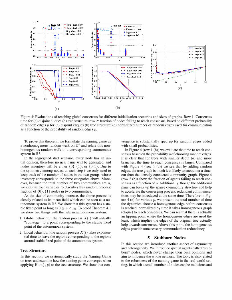
Simulation Results. Figure 4 (row 1 (a)) shows the conver-gence time for different values of p under different initialscenarios on graphs of size n. For each setting we run thesimulation multiple times and plot the time to reach consen-sus for each run as a dot in the figure. In certain situations itis hard to reach consensus even after a long time. Thereforewe set 107 as the time-out criteria – i.e., if no consensus isreached after 107 rounds and we stop the simulation. FromFigure 4 (row 1 (a)) we can see that when p is smaller it isharder to reach consensus for all situations. When p is suf-ficiently small all situations may hit the timeout conditionbefore consensus is reached. In addition, the threshold of pwhich allows this happen is larger for the “segregated” ini-tial setup compared to the empty initial setup. Similarly, forgraphs of larger size it is easier to hit the time out condition.When p > 0.2 the time to reach consensus for all situationsis small so we chose not to plot it.

To further analyze the naming game behavior when p is inbetween [0, 0.25], we show in Figure 4 (row 2 (a)) the frac-tion of trials failing to reach consensus (before timing out)with different values of p. It is clear that for the empty startinitial condition, the game will time out at about p = 0.24,while for the segregated start case, the game will time outwhen p is around 0.26. This threshold value changes withthe size of the local community.

Curiously, for the “empty” start, graphs with smaller sizesare more likely to encounter timeouts than their larger coun-terparts. This may be because the smaller size of each com-munity results in a greater chance of quickly reaching localconsensus, which resembles the segregated start scenario.Therefore, it takes longer for graphs with smaller sizes tobreak the local consensus and escape the so called “stuck”situation.

However, for the segregated start, it immediately startswith the “worst” case setting where the two communitieshave diverging opinions, so overall it takes longer to leave“stuck” situation compared with graphs of the same size inthe “empty” start scenario. Additionally, graphs with largersizes in the segregated setting more easily encounter a time-out. This may be because larger graphs occasionally time outeven if they are not really “stuck” because they take longerto reach consensus in any event.

Theoretical Analysis. Next we will analyze the consensustime for the naming game on Hom(G, p) where G has 2nagents divided into two equally sized disconnected commu-nities with segregated start.

Theorem 4.1. Let G be the disjoint union of two n cliques,each of size n. Then for the segregated start naming gameon Hom(G, p), there exists a constant p0 ≈ 0.110 such thatif 0 ≤ p < p0 the expected consensus time is exp(Ω(n)).

Here we sketch a proof of theorem. A full proof appearsin the appendix.

(a) (b)

(c)

Figure 4: Evaluations of reaching global consensus for different initialization scenarios and sizes of graphs. Row 1: Consensustime for (a) disjoint cliques (b) tree structure; row 2: fraction of nodes failing to reach consensus, based on different probabilityof random edges p for (a) disjoint cliques (b) tree structure; (c) normalized number of random edges used for communicationas a function of the probability of random edges p.

To prove this theorem, we formulate the naming game asa nonhomogenous random walk on Z4 and relate this non-homogenous random walk to a corresponding autonomoussystem in R4.

In the segregated start scenario, every node has an ini-tial opinion, therefore no new name will be generated, andnodes inventory will be either 0, 1, or 0, 1. Due tothe symmetry among nodes, at each step t we only need tokeep track of the number of nodes in the two groups whoseinventory corresponds to the three categories above. More-over, because the total number of two communities are n,we can use four variables to discribes this random process:fraction of 0, 1 nodes in two communities.

As the size of community increase, the above process isclosely related to its mean field which can be seen as a au-tonomous system in R4. We show that this system has a sta-ble fixed point as long as 0 ≤ p < p0. To proof Theorem 4.1we show two things with the help in autonomous system:

1. Global behaviour: the random process X(t) will initially“converge” to a point corresponding to the stabile fixedpoint of the autonomous system.

2. Local behaviour: the random processX(t) takes exponen-tial time to leave the regions corresponding to the regionsaround stable fixed point of the autonomous system.

Tree StructureIn this section, we systematically study the Naming Gameon trees and examine how the naming game converges whenapplying Hom(·, p) to the tree structure. We show that con-

vergence is substantially sped up for random edges addedwith small probabilities.

In Figure 4 (row 1 (b)) we evaluate the time to reach con-sensus based on the probability p of choosing random edges.It is clear that for trees with smaller depth (d) and morebranches, the time to reach consensus is larger. Comparedwith Figure 4 (row 1 (a)) we see that by adding randomedges, the tree graph is much less likely to encounter a time-out than the densely connected community graph. Figure 4(row 2 (b)) show the fraction of agents failing to reach con-sensus as a function of p. Additionally, though the additionalpairs can break up the sparse community structure and helpto accelerate the converging process, redundant communica-tions may be introduced at the same time. Therefore in Fig-ure 4 (c) for various p, we present the total number of timethe dynamics choose a homogenous edge before consensusis reached, normalized by time it takes homogeneous graph(clique) to reach consensus. We can see that there is actuallyan tipping point where the homogenous edges are used theleast, which implies the edges of the original tree actuallyhelp towards consensus. Above this point, the homogeneousedges provide unnecessary communication redundancy.

5 Stubborn NodesIn this section we introduce another aspect of asymmetryand heterogeneity. We introduce special agents called “stub-born” nodes, which never change their own opinions andaim to influence the whole network. The topic is also relatedto the robustness of the naming game in the real world set-ting, in which a small number of nodes can be malicious and

(a) (b) (c)

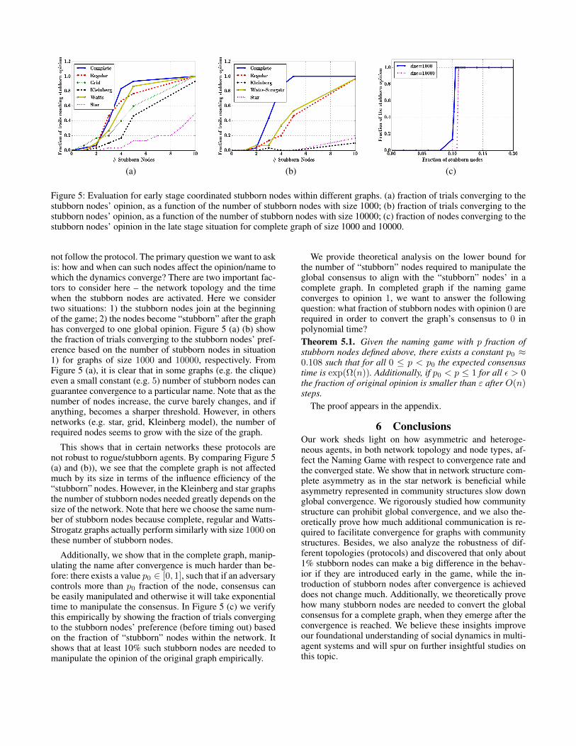
Figure 5: Evaluation for early stage coordinated stubborn nodes within different graphs. (a) fraction of trials converging to thestubborn nodes’ opinion, as a function of the number of stubborn nodes with size 1000; (b) fraction of trials converging to thestubborn nodes’ opinion, as a function of the number of stubborn nodes with size 10000; (c) fraction of nodes converging to thestubborn nodes’ opinion in the late stage situation for complete graph of size 1000 and 10000.

not follow the protocol. The primary question we want to askis: how and when can such nodes affect the opinion/name towhich the dynamics converge? There are two important fac-tors to consider here – the network topology and the timewhen the stubborn nodes are activated. Here we considertwo situations: 1) the stubborn nodes join at the beginningof the game; 2) the nodes become “stubborn” after the graphhas converged to one global opinion. Figure 5 (a) (b) showthe fraction of trials converging to the stubborn nodes’ pref-erence based on the number of stubborn nodes in situation1) for graphs of size 1000 and 10000, respectively. FromFigure 5 (a), it is clear that in some graphs (e.g. the clique)even a small constant (e.g. 5) number of stubborn nodes canguarantee convergence to a particular name. Note that as thenumber of nodes increase, the curve barely changes, and ifanything, becomes a sharper threshold. However, in othersnetworks (e.g. star, grid, Kleinberg model), the number ofrequired nodes seems to grow with the size of the graph.

This shows that in certain networks these protocols arenot robust to rogue/stubborn agents. By comparing Figure 5(a) and (b)), we see that the complete graph is not affectedmuch by its size in terms of the influence efficiency of the“stubborn” nodes. However, in the Kleinberg and star graphsthe number of stubborn nodes needed greatly depends on thesize of the network. Note that here we choose the same num-ber of stubborn nodes because complete, regular and Watts-Strogatz graphs actually perform similarly with size 1000 onthese number of stubborn nodes.

Additionally, we show that in the complete graph, manip-ulating the name after convergence is much harder than be-fore: there exists a value p0 ∈ [0, 1], such that if an adversarycontrols more than p0 fraction of the node, consensus canbe easily manipulated and otherwise it will take exponentialtime to manipulate the consensus. In Figure 5 (c) we verifythis empirically by showing the fraction of trials convergingto the stubborn nodes’ preference (before timing out) basedon the fraction of “stubborn” nodes within the network. Itshows that at least 10% such stubborn nodes are needed tomanipulate the opinion of the original graph empirically.

We provide theoretical analysis on the lower bound forthe number of “stubborn” nodes required to manipulate theglobal consensus to align with the “stubborn” nodes’ in acomplete graph. In completed graph if the naming gameconverges to opinion 1, we want to answer the followingquestion: what fraction of stubborn nodes with opinion 0 arerequired in order to convert the graph’s consensus to 0 inpolynomial time?Theorem 5.1. Given the naming game with p fraction ofstubborn nodes defined above, there exists a constant p0 ≈0.108 such that for all 0 ≤ p < p0 the expected consensustime is exp(Ω(n)). Additionally, if p0 < p ≤ 1 for all ε > 0the fraction of original opinion is smaller than ε after O(n)steps.

The proof appears in the appendix.

6 ConclusionsOur work sheds light on how asymmetric and heteroge-neous agents, in both network topology and node types, af-fect the Naming Game with respect to convergence rate andthe converged state. We show that in network structure com-plete asymmetry as in the star network is beneficial whileasymmetry represented in community structures slow downglobal convergence. We rigorously studied how communitystructure can prohibit global convergence, and we also the-oretically prove how much additional communication is re-quired to facilitate convergence for graphs with communitystructures. Besides, we also analyze the robustness of dif-ferent topologies (protocols) and discovered that only about1% stubborn nodes can make a big difference in the behav-ior if they are introduced early in the game, while the in-troduction of stubborn nodes after convergence is achieveddoes not change much. Additionally, we theoretically provehow many stubborn nodes are needed to convert the globalconsensus for a complete graph, when they emerge after theconvergence is reached. We believe these insights improveour foundational understanding of social dynamics in multi-agent systems and will spur on further insightful studies onthis topic.

ReferencesBackstrom, L.; Huttenlocher, D.; Kleinberg, J.; and Lan, X.2006. Group formation in large social networks: member-ship, growth, and evolution. In Proceedings of the 12th ACMSIGKDD international conference on Knowledge discoveryand data mining, 44–54. ACM.Baronchelli, A.; Felici, M.; Loreto, V.; Caglioti, E.; andSteels, L. 2006a. Sharp transition towards shared vocabular-ies in multi-agent systems. Journal of Statistical Mechanics:Theory and Experiment 2006(06):P06014.Baronchelli, A.; Loreto, V.; DallAsta, L.; and Barrat, A.2006b. Bootstrapping communication in language games:Strategy, topology and all that. In Proceedings of the 6th In-ternational Conference on the Evolution of Language, vol-ume 2006, 11–18. World Scientific Press.Baronchelli, A.; Dall’Asta, L.; Barrat, A.; and Loreto, V.2007. The role of topology on the dynamics of the nam-ing game. The European Physical Journal Special Topics143(1):233–235.Baronchelli, A.; Loreto, V.; and Steels, L. 2008. In-depthanalysis of the naming game dynamics: the homogeneousmixing case. International Journal of Modern Physics C19(05):785–812.Bollobas, B. 1998. Random graphs. In Modern GraphTheory. Springer. 215–252.Brighton, H., and Kirby, S. 2001. The survival of the small-est: Stability conditions for the cultural evolution of com-positional language. In European Conference on ArtificialLife, 592–601. Springer.Centola, D., and Baronchelli, A. 2015. The spontaneousemergence of conventions: An experimental study of cul-tural evolution. Proceedings of the National Academy ofSciences 112(7):1989–1994.Dall’Asta, L.; Baronchelli, A.; Barrat, A.; and Loreto, V.2006. Agreement dynamics on small-world networks. EPL(Europhysics Letters) 73(6):969.Ellison, G. 2000. Basins of attraction, long-run stochasticstability, and the speed of step-by-step evolution. The Re-view of Economic Studies 67(1):17–45.Franks, H.; Griffiths, N.; and Jhumka, A. 2013. Manipu-lating convention emergence using influencer agents. Au-tonomous Agents and Multi-Agent Systems 26(3):315–353.Gong, T.; Ke, J.; Minett, J. W.; and Wang, W. S. 2004. Acomputational framework to simulate the coevolution of lan-guage and social structure. In Artificial Life IX: Proceedingsof the 9th International Conference on the Simulation andSynthesis of Living Systems, 158–64.Hurford, J. R. 1989. Biological evolution of the saussureansign as a component of the language acquisition device. Lin-gua 77(2):187–222.Kleinberg, J. 2000. The small-world phenomenon: An al-gorithmic perspective. In Proceedings of the thirty-secondannual ACM symposium on Theory of computing, 163–170.ACM.

Lu, Q.; Korniss, G.; and Szymanski, B. K. 2009. The nam-ing game in social networks: community formation and con-sensus engineering. Journal of Economic Interaction andCoordination 4(2):221–235.Nowak, M. A., and Krakauer, D. C. 1999. The evolution oflanguage. Proceedings of the National Academy of Sciences96(14):8028–8033.Nowak, M. A.; Plotkin, J. B.; and Jansen, V. A. 2000.The evolution of syntactic communication. Nature404(6777):495–498.Nowak, M. A.; Plotkin, J. B.; and Krakauer, D. C. 1999. Theevolutionary language game. Journal of Theoretical Biology200(2):147–162.Pickering, W., and Lim, C. 2016. Solution of the multistatevoter model and application to strong neutrals in the naminggame. Physical Review E 93(3):032318.Steels, L., and McIntyre, A. 1998. Spatially distributed nam-ing games. Advances in complex systems 1(04):301–323.Steels, L. 1995. A self-organizing spatial vocabulary. Arti-ficial life 2(3):319–332.Steels, L. 2005. The emergence and evolution of linguisticstructure: from lexical to grammatical communication sys-tems. Connection science 17(3-4):213–230.Strogatz, S. H. 2014. Nonlinear dynamics and chaos: withapplications to physics, biology, chemistry, and engineering.Westview press.Watts, D. J., and Strogatz, S. H. 1998. Collective dynamicsof small-worldnetworks. Nature 393(6684):440–442.Wormald, N. C. 1995. Differential equations for randomprocesses and random graphs. The annals of applied proba-bility 1217–1235.

A PreliminaryOur technique to prove Theorem 4.1 and Theorem 5.1 whichcombines mean field approximation and stability of differen-tial systems. We think our technique will apply to other set-tings as well. At a very high level: first we relate the randomprocess to a differential equation, and next we characterizethe long term behaviour of differential equation.

Mean field approximationThere is extensive literature about stochastic processes andits mean field approximation e.g. (Ellison 2000). Given anonhomogeneous random walk X(t) in Z` we can associatethe behavior of it with the corresponding differential equa-tion in R`. Formally, let Xn(t) be a discrete time Markovchain on Z` with parameter n which is time-homogeneousand the increments of the walk are uniformly bounded by β.As a result, random vectors Xn(t + 1) − Xn(t) have welldefined moments, which depend on X(t) and n. In particu-lar, an important quantity is the one-step mean drift vectorFn : R` → R` defined to be

Fn(X) = E[Xn(t+ 1)Xn(t)|Xn(t) = X]. (1)

In particular if there exists a function f independent of nsuch that Fn(X) = f(Xn ), then there is a close relationshipbetween X and the x which we define as a solution of thefollowing autonomous differential system

x′ = f(x) (2)

with initial condition x(0) = X(0)/n.The following theorem shows that the differential equa-

tion approximates the original random walk X(t) such thatX(t) ≈ nx( tn ) under proper conditions.

Theorem A.1 (Wormald’s method (Wormald 1995)). For1 ≤ ` ≤ a where a is fixed, let y` : S(n)+ → R andf` : Ra+1 → R such that for some constant C0 and all`, |y`(ht)| < C0n for all ht ∈ S(n)+ and n. Let Y`(t) de-note the random counterpart of y`(ht). Assume the follow-ing three conditions hold:

1. (Boundedness) For some functions β = β(n) ≥ 1 andγ = γ(n), the probability that

max`|Y`(t+ 1)− Y`(t)| ≤ β

conditional upon Ht, is at least 1− γ for t < TD.2. (Trend) For some function λ1 = λ1(n) = o(1), for all` ≤ a

|E[Y`(t+ 1)− Y`(t)|Ht]− f`(t

n,Y1(t)

n, ...,

Ya(t)

n) ≤ λ1

for t ≤ TD.3. (Lipschitz) Each function f` is continuous, and satisfies a

Lipschitz condition, on

D ∩ (t, z1, ..., za) : t ≥ 0,

with the same Lipschitz constant for each `.

Then the following are true.

1. For (0, z1, ..., za) ∈ D the system of differential equations

dz`dx− f`(x, z1, .., za), ` = 1, ..., z (3)

have a unique solution in D for z` : R → R passingthrough z`(0) = z` for 1 ≤ ` ≤ a, which extends topoints arbitrarily close to the boundary of D;

2. Let λ > λ1 +C0nγ with λ = o(1). For a sufficiently largeconstant C with probability 1−O(nγ + β

λ exp(−nλ3

β3 )),

Y`(t) = nz`(t

n) +O(λn) (4)

uniformly for 0 ≤ t ≤ σn and for each ` where z`(x)

is the solution in Equation (3) with z` = Y`(t)n , and σ =

σ(n) is the supremum of those x to which the solution canbe extended before reaching within `∞-distanceCλ of theboundary of D.

Stability of autonomous systemStability capture the long term behaviour of (2). Here issome notation: a point x ∈ R` is called an equilibriumpoint of system (2) if f(x) = 0. Moreover the equilib-rium x is asymptotically stable if ∀ε > 0,∃δ > 0 such that||x(0)− x|| ≤ δ ⇒ ||x(t)− x|| ≤ ε,∀t and ∃δ > 0 such thatlimt→∞ ||x(t)− x|| = 0. The stability of the system can bedetermined by the linearization of the system which is statedbelow.

Theorem A.2 (Lyapunov’s indirect method (Strogatz2014)). Let x∗ be an equilibrium point for x′ = f(x) wheref : D → Rd is continuously differentiable andD is a neigh-borhood of x∗. Let A = ∂f

∂x |x=x∗ then x∗ is asymptoticallystable ifA is Hurwitz, that isRe(λi) < 0 for all eigenvaluesof A.

Moreover, there exists an close set U ⊆ D and x∗ ∈ Uand a potential function V : U → R such that V (x∗) = 0,and V (x) > 0, ddt (V (x)) < 0 for x ∈ U \ x∗.

However the above theorem only captures the behaviourof x when it is close enough to the stabile fixed point x∗. Onthe other hand for global stability, the following theoremsis quite useful when system (2) is in the plane. To state thetheorem we need to introduce more terminology. A set isbounded if it is contained in some cycle x ∈ R2|||x− α <C for some α ∈ R2 and C > 0. A point p ∈ R2 is calledan ω-limit point of the trajectory Γz0 = z(t)|t ≥ 0, z(0) =z0 of the system (2) if there is a sequence tn → ∞ suchthat limn→∞ x(tn) = p.

Theorem A.3 (Poincare-Bendixon Theorem (Strogatz2014)). Let z′ = H(z) be a system of differential equa-tions defined on E an open subset in R2 where H is differ-entiable. Suppose a forward orbit with initial condition z0

Γz0 = z(t)|t ≥ 0, z(0) = z0 is bounded. Then either

• ω(z0) contains a fixed point• ω(z0) is a periodic orbit

The following theorem gives us a sufficient condition fornonexistence of periodic orbit

Theorem A.4 (Bendixson’s Criteria (Strogatz 2014)). LetH be differentiable in E where E is a simply connected re-gion in R2. If the divergence of the vector field H is notidentically zero and does not change sign in E then z′H(x)has no closed periodic orbit lying entirely in E.

Note that the theorem only holds for two dimensions sys-tem and fails in general.

B Main ResultsThe main idea used to prove both Theorem 4.1 and Theorem5.1 is to show the existence of a stable fixed point x∗ ofthe solution to differential system (2) and then to relate thisstable fixed point to the nonhomogeneous random walk (1)by showing:

1. Global behaviour: the random process X(t) will initially“converge” to a point corresponding to the stabile fixedpoint of the autonomous system.

2. Local behaviour: random process X(t) takes exponentialtime to leave the region corresponding to a regions aroundstabile fixed point of the autonomous system.Here we prove a auxiliary theorem for the second part.

Theorem B.1. If x∗ is an asymptotically stable equilibriumof (2), given a closed setU containing x∗ there exists ra > 0such that in system (1) if ||X(t0)/n− x∗|| ≤ ra then

E[arg minτ>t0

X(τ) 6∈ U∣∣||X(t0)/n−x∗|| ≤ ra] = exp(Ω(n)).

To prove Lemma B.1, we use the second part of Lya-punov’s indirect method Theorem A.2, which shows the ex-istence of a potential function V (x) at some region aroundthe asymptotically stable fixed point in system (2) such thatthe value of potential function is strictly decrease along thetrajectory. On the other hand, the counterpart of that poten-tial function in (1) will be a supermartingale V (X(t)) andwe use the optional stopping time to show that it takes anexponential time for the supermartingale to increase by con-stant.

Proof of Lemma B.1. By Theorem A.2, we know that thereexists a potential function V and an open region U ⊆ Dsuch that V (x∗) = 0, and V (x) > 0, ddt (V (x)) < 0 forx ∈ U \ x∗. Now we consider a random process

W (i) = V

(X(i)

n

)and the conditional expectation is

E[W (i+ 1)−W (i)|X(i)]

=E[V (X(i+ 1)

n)− V (

X(i)

n)|X(t)]

=∇V (X(i)

n) · (E[X(i+ 1)−X(i)|X(i)]

n) +O(

1

n2)

=∇V (X(i)

n) ·f(X(i)

n )

n+O(

1

n2)

=1

n

d

dtV (x)

∣∣∣x=

X(i)n

+O(1

n2) (5)

ThereforeW (i) is a supermartingale such that E[W (i+1)−W (i)|X(i)] < 0 when X(t)

n ∈ U \ x∗ and n is largeenough.

The idea is to use the optional stopping theorem by prov-ing the process X(t) is not likely to pass through the an-nulus Brb \ Bra for some properly choosen ra, rb. Herewe need to use the properties of the potential function Vfrom Theorem A.2. Note that U is open, there exists rb > 0such that a open set Brb = ||x − x∗|| < rb ⊆ U . Be-cause the boundary U \ Brb is compact and V is continu-ous, there exists minx∈Brb

V (x) which is denoted as lb. Onthe other hand, because V (x∗) = 0 and V is continuous,there exists a close set Bra where 0 < ra < rb such thatla = maxx∈ ¯Bra

V (x) ≤ 0.3lb.Given such ra, rb if X(t0)/n ∈ Bra at some time t0 and

the system leaves the stable region U at time t1 > t0 thereexists σ,τ when n is large enough such that

τ = arg mint0<t<t1

X(t)/n ∈ U \Brb

σ = arg maxt0<s<τ

X(s)/n ∈ Bra

which gives us

W (σ) < 0.5la, and W (τ) ≥ lb

Moreover by the definition of σ, τ , for all σ ≤ t < τ therandom process X(t) would stay in the annulus Brb \ Bra .Therefore for all t such that σ ≤ t < τ , we have W (t) is astrict supermartingale

W (t) =1

n

d

dtV (x)

∣∣∣x=

X(i)n

+O(1

n2) =−h2n

< 0

where constant −h = maxx∈Brb\Bra

ddtV (x)

∣∣∣x< 0 since

the annulus is compact.Therefore by standard optional stopping time theorem

with initial state W (σ + 1) where la < W (σ + 1) < lb theaverage time for W (t) to hit W (t) ≥ lb is exp(Ω(hn)) =exp(Ω(n)).

C Proof of Theorem 4.1Recall that we want to formulate the naming game as nonho-mogenous random walk on Z4 and relate this nonhomoge-nous random walk to a correpsonding autonomous system inR4 to study consensus time. Note that we can use four vari-ables to describe this random process: fraction of 0, 1nodes in two communities by following notations.

At community1 community20 R1(t) R2(t)1 B1(t) B2(t)0, 1 M1(t) M2(t)

Since n = R1(t) + B1(t) + M1(t) = R2(t) +B2(t) + M2(t) for all t, it’s sufficient to consider X(t) =(R1(t), B1(t), R2(t), B2(t)) in Z4 with initial state X(0) =(n, 0, 0, n) and the naming game reaches consensus at Twhen X(T ) = (n, 0, n, 0) or (0, n, 0, n).

We can now define F (·) as the mean field of this system(as in Equation (1)):

F (X(t)) = E[X(t+ 1)−X(t)|X(t)]. (6)

Our approach to understand the behavior of X is mainlyinspired by the stability property of nonlinear autonomoussystems. We define f(·) such that Fn(X) = f(Xn ) and thenwe can relate the nonhomogeneous random walk X to thesolution of x′ = f(x) as in (2).

Intuitively we will prove that there exists p such that thesystem has an “undesirable” asymptotically stable points x∗(which will be defined mathematically in appendix)

x∗ = (r∗, b∗, b∗, r∗)

where r∗ = e2+√−4e+6e2−e4

2e , b∗ = e2−√−4e+6e2−e4

2e andp = 2

3 (1 − e) such that the random process X(t) in Equa-tion (6) will

1. Reach some region of nx∗.

2. Given X(T0) is in some region of nx∗ the expected con-sensus time of the corresponding naming game is expo-nential in the size of each group exp(Ω(n)).

These two conclusions can be proved by the following twolemmas, respectively and the proof of Theorem 4.1 followsdirectly from the above two Lemmas.

Lemma C.1. Given the naming game defined above, if0 ≤ p < 4−2

√3

3 ≈ 0.178 given arbitrary constant ra > 0the random walkX(t) will converge to x∗. That is there existT0 = O(n) such that ||X(T0)/n− x∗|| ≤ ra with probabil-ity 1−O( logn

exp( −n

log3 n))

Lemma C.2. Given the naming game defined above, thereexists a constant p0 ≈ 0.110 such that for all 0 ≤ p < p0

there exists some constant ra > 0 such that if ||X(T0)/n −x∗|| ≤ ra then the consensus time is exp(Ω(n))

Now we need to quantify the evolution of this process.Recalled that our naming game defined in (6)

E[R1(t+ 1)−R1(t)|X(t)] =1

2

(1− R1

n− 2

B1

n+ (

B1

n)2)

+p

2(−R1

2n+B1

n+R2

2n− B2

n− (

B1

n)2 − 3R1B2

2n2− B1R2

2n2)

E[B1(t+ 1)−B1(t)|X(t)] =1

2

(1− B1

n− 2

B1

n+ (

R1

n)2)

+p

2(−B1

2n+R1

n+B2

2n− R2

n− (

R1

n)2 − 3B1R2

2n2− R1B2

2n2)

E[R2(t+ 1)−R2(t)|X(t)] =1

2

(1− R2

n− 2

B2

n+ (

B2

n)2)

+p

2(−R2

2n+B2

n+R1

2n− B1

n− (

B2

n)2 − 3R2B1

2n2− B2R1

2n2)

E[B2(t+ 1)−B2(t)|X(t)] =1

2

(1− B2

n− 2

B2

n+ (

R2

n)2)

+p

2(−B2

2n+R2

n+B1

2n− R1

n− (

R2

n)2 − 3B2R1

2n2− R2B1

2n2)

R1(0) = n,B1(0) = 0, R2(0) = 0, B2(0) = n

has corresponding autonomous differential system as fol-low.

r′1 =1

2

(1− r1 − 2b1 + b21

+p

2(−1

2r1 + b1 +

1

2r2 − b2 − b21 −

3

2r1b2 −

1

2b1r2)

b′1 =

1

2

(1− b1 − 2r1 + r2

1

+p

2(−1

2b1 + r1 +

1

2b2 − r2 − r2

1 −3

2b1r2 −

1

2r1b2)

r′2 =

1

2

(1− r2 − 2b2 + b22

+p

2(−1

2r2 + b2 +

1

2r1 − b1 − b22 −

3

2r2b1 −

1

2b2r1)

b′2 =

1

2

(1− b2 − 2r2 + r2

2

+p

2(−1

2b2 + r2 +

1

2b1 − r1 − r2

2 −3

2b2r1 −

1

2r2b1)

r1(0) = 1, b1(0) = 0, r2(0) = 0, b2(0) = 1 (7)

Proof of Lemma C.2With Theorem B.1, to prove Lemma C.2, it is sufficient toprove x∗ is a stable fixed point.

Proof of Lemma C.2. With Theorem A.2, it is sufficient toshow all the eigenvalues of A = ∂f

∂x |x=x∗ are negative. Byelementary computation, the eigenvalues of A are

−e− 5

6−D1,

−e− 5

6+D1

e2 − 3

2−D2,

e2 − 3

2+D2

where p = 23 (1− e) and

D1 =1

6

√(1− e)(−8e4 − 36e3 + 7e2 + 153e+ 64)

e

D2 =1

2

√(1− e)(−e3 − 5e2 + e+ 25)

Therefore A is Hurwitz and x∗ is asymptotically stable ife > 0.835 and 0 ≤ p < 0.110

Proof of Lemma C.1To proof Lemma C.1 we prove two claims:

1. The solution x to the differential equation in (7) convergesto x∗;

2. the limit behavior of random process in (6) can be approx-imated by x in (7), that is limn→∞X(nt)/n ≈ x(t).

With these two claims we can conclude given any ra > 0there exists t0 such that ||X(t)/n − x∗|| < ra for allt > t0 with high probability. For the first claim we usePoincare-Bendixon Theorem A.3 and use Wormald’s differ-ential equation method A.1 to prove the second.

Proof of Lemma C.1. First, by the symmetry of the systemand initial conditions r1 = b2 = 1 and b1 = r2 = 0. wecan assume that r1(t) = b2(t) and b1(t) = r2 for all t ≥ 0,and the system of differential equations is equivalent to thefollowing

r′ = (1− r − 2b+ b2) +1− e

2(b− r − b2 − r2)

b′ = (1− b− 2r + r2) +1− e

2(r − b− r2 − b2)

where r(0) = 1, and b(0) = 0

where r(t) = r1(t) = b2(t) b(t) = r1(t) = b2(t) andp = 1−e

3 , and the system will have stable fixed point r∗ =e2+√−4e+6e2−e4

2e and b∗ = e2−√−4e+6e2−e4

2e , and we take

x∗ = (r∗, b∗, b∗, r∗)

Note that such x∗ exists if −4 + 6e − e3 ≥ 0, i.e. 0 ≤ p ≤4−2√

33 ≈ 0.178.To apply Theorem A.3 in (8), we need to show the orbit

of (r, b) is bounded and there is no periodic cycle. It is easyto see that r(t), b(t) are bounded in interval [0, 1]. More-over because if r(t) = b(t) for some t then r(t′) = b(t′)for all t′ ≥ t, we have r(t) ≥ b(t). Combining these twoobservations we have (r, b) is bounded in Ω = (r, b)|r ≥b, 0 ≤ r, b ≤ 1. On the other hand, because ∇ · H =−2 + 1−e

2 (−2− 2r − 2b) < 0∀(r, b) ∈ Ω which, by Theo-rem A.4, proves there is no closed orbit. Therefore we haveproven the first claim: limt→∞(r(t), b(r)) = (r∗, b∗) byTheorem A.3. Furthermore in (7) we have

||x(t)− x∗|| < 0.5ra∀t > t0. (8)

For the second claim, we want to show the original pro-cess in (6) can be approximated by (7). It is not hard toshow that the process is bounded by β = 1 and γ = 0,and by taking λ = O( 1

log(n) ) we have with probability1−O(log n exp(− n

log3 n)

X(nt)/n = x(t) +O(1

log n) (9)

in terms of each component.Combining (8) and (9) we have with probability 1 −

O(log n exp(− nlog3 n

))

||X(nt)/n− x∗|| ≤ ra,∀t > t0

when n is large enough.

D Proof of Theorem 5.1We define stubborn node which has different behavior innaming game. A node s is stubborn if its inventory willnot change the process At(s) = A0(s) even when it is thespeaker or listener, and we call node s is stubborn node withA0(s), and we call other node as ordinary nodes. Here weconsider that on completed graph if the naming game is al-ready consensus on opinion 1. The Theorem 5.1 gives a wayto understand the following question: how many nodes stub-born with opinion 0 do we make in order to change the graphconsensus on opinion 0 in polynomial time?

Theorem D.1 (Restate theorem 5.1). Given the naminggame with p fraction of stubborn nodes defined above, thereexists a constant p0 ≈ 0.108 such that for all 0 ≤ p < p0

the expected consensus time is exp(Ω(n)). Additionally, ifp0 < p ≤ 1 for all ε > 0 the fraction of original opinion issmaller than ε after O(n) steps.

Similar to the proof of theorem 4.1, we formulate thisprocess as nonhomogenous random walk on Z2 and relatethis nonhomogenous random walk to a correpsonding au-tonomous system in R2 to study consensus time.

Model DescriptionGiven a completed graph G which has n nodes and theweight of every pair of node is uniform, if every nodes con-sensus on 1, we want to make p fraction of nodes stubbornon 0, and all the set of stubborn nodes S such that |S| = pn.That is ∀s ∈ S,A0(s) = 0 and for all ordinary nodev ∈ V (G) \ S,A0(v) = 0.

Because the symmetry of the completed graph, only thenumber of stubborn nodes matters, and we apply the samemethod in theorem 4.1 to simplify the notations. At time t,we defineX(t) = (R(t), B(t)) as our state of Markov chainwhereR(t) the number of ordinary node with inventory 0,B(t) the number of ordinary node with inventory 1 andM(t) be the number of ordinary node with inventory 0, 1.Moreover we use n to denote the number of ordinary nodes,n = |V (G) \ S| = (1− p)n. Here we have

E[R(t+ 1)−R(t)|X(t)]

=(1− p)2(R

n

M

n+ (

M

n)2 − R

n

B

n) + p(1− p)3

2

M

nE[B(t+ 1)−B(t)|X(t)]

=(1− p)2(B

n

M

n+ (

M

n)2 − R

n

B

n)− p(1− p)B

n

and the corresponding autonomous differential system is

r′ =(1− p)2(rm+m2 − rb) + p(1− p)3

2m

b′ =(1− p)2(bm+m2 − rb)− p(1− p)b

ProofsSimilar to theorem 4.1, when p < 0.108 it is striaghtforwardto show there exists a stable fixed point x∗ 6= (1, 0) andderived the following two lemmas to prove the first part ofTheorem 5.1.Lemma D.1. Given the naming game defined above, thereexists p0 ≈ 0.108 such that for all constant 0 ≤ p < p0 thereexists some constant ra > 0 such that if ||X(T0)/n−x∗|| ≤ra then the consensus time is exp(Ω(n))

Lemma D.2. Given the naming game defined above, if con-stant 0 ≤ p < 0.108 given arbitrary constant ra > 0 therandom walk X(t) will converge to x∗. That is there existsT0 = O(n) such that ||X(T0)/n− x∗|| ≤ ra with probabil-ity 1−O( logn

exp( −n

log3 n))

For the second part of Theorem 5.1, since if p > p0 theconsensus point,c∗ = (1, 0) is the only fixed point of thesystem, we can use similar technique in Lemma C.1 andTheorem B.1 to prove given arbitrary small constant ε > 0,b(t) ≤ ε for t = O(n).