engineering mathematics – i - · pdf fileengineering mathematics – i dr. v....
TRANSCRIPT

Engineering Mathematics – I Dr. V. Lokesha
10 MAT11
1
2011
Engineering Mathematics – I
(10 MAT11)
LECTURE NOTES (FOR I SEMESTER B E OF VTU)
VTU-EDUSAT Programme-15
Dr. V. Lokesha Professor and Head
DEPARTMENT OF MATHEMATICS ACHARYA INSTITUTE OF TECNOLOGY
Soldevanahalli, Bangalore – 90
Engineering Mathematics – I Dr. V. Lokesha
10 MAT11
2
2011
ENGNEERING MATHEMATICS – I
Content
CHAPTER
UNIT I DIFFERENTIAL CALCULUS – I
UNIT II DIFFERENTIAL CALCULUS – II
UNIT III DIFFERENTIAL CALCULUS – III
Engineering Mathematics – I Dr. V. Lokesha
10 MAT11
3
2011
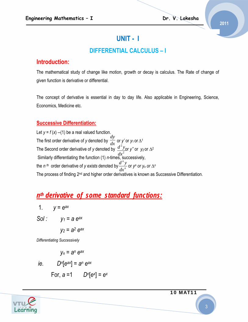
UNIT - I DIFFERENTIAL CALCULUS – I
Introduction: The mathematical study of change like motion, growth or decay is calculus. The Rate of change of given function is derivative or differential. The concept of derivative is essential in day to day life. Also applicable in Engineering, Science, Economics, Medicine etc.
Successive Differentiation: Let y = f (x) --(1) be a real valued function. The first order derivative of y denoted by or y’ or y1 or ∆1 The Second order derivative of y denoted by or y’’ or y2 or ∆2 Similarly differentiating the function (1) n-times, successively, the n th order derivative of y exists denoted by or yn or yn or ∆n The process of finding 2nd and higher order derivatives is known as Successive Differentiation.
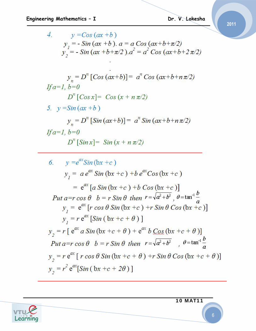
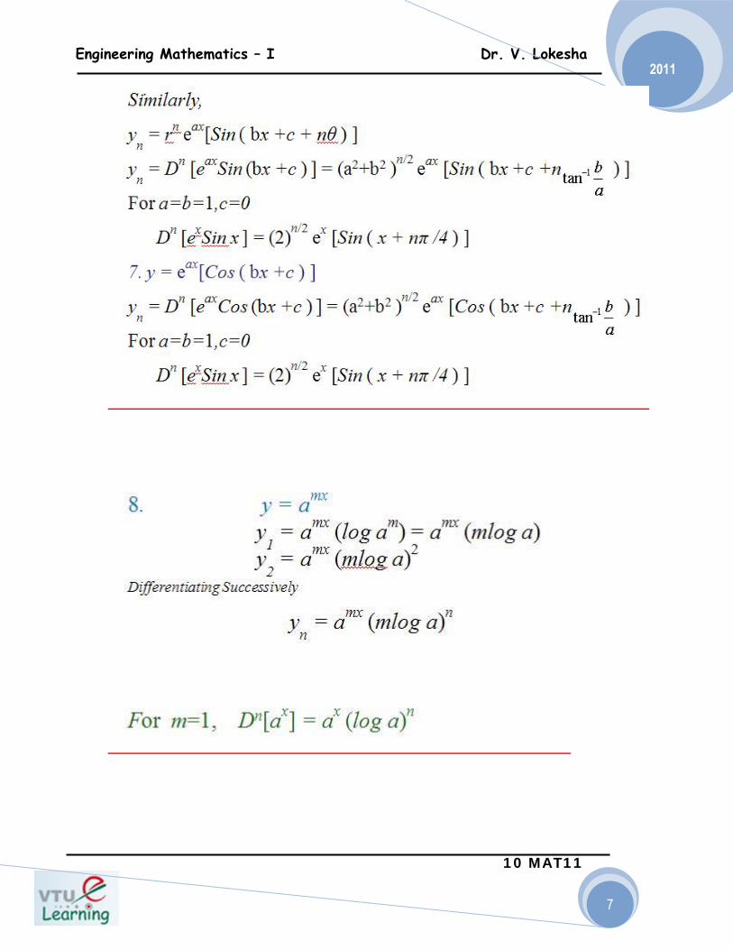
nth derivative of some standard functions: 1. y = eax Sol : y1 = a eax y2 = a2 eax Differentiating Successively yn = an eax ie. Dn[eax] = an eax For, a =1 Dn[ex] = ex
dxdy
2
2
dxyd
n
n
dxyd
Engineering Mathematics – I Dr. V. Lokesha
10 MAT11
4
2011
Engineering Mathematics – I Dr. V. Lokesha
10 MAT11
5
2011
Engineering Mathematics – I Dr. V. Lokesha
10 MAT11
6
2011
Engineering Mathematics – I Dr. V. Lokesha
10 MAT11
7
2011

Engineering Mathematics – I Dr. V. Lokesha
10 MAT11
8
2011
Leibnitz’s Theorem : It provides a useful formula for computing the nth derivative of a product of two functions. Statement : If u and v are any two functions of x with un and vn as their nth derivative. Then the nth
derivative of uv is
(uv)n = u0vn + nC1 u1vn-1 + nC2u2vn-2 + …+nCn-1un-1v1+unv0 Note : We can interchange u & v (uv)n = (vu)n,
nC1 = n , nC2 = n(n-1) /2! , nC3= n(n-1)(n-2) /3! …
1. Find the nth derivations of eax cos(bx + c) Solution: y1 = eax – b sin (bx +c) + a eax cos (b x + c), by product rule. .i.e, y1 = eax ( ) ( )[ ]cbxsinbcbxcosa +−+
Let us put a = r cos θ , and b = r sin θ .
∴ 222 rba =+ and tan a/b=θ
.ie., 22 bar += and θ = tan-1 (b/a)
Now, [ ])cbxsin(sinr)cbxcos(cosrey ax1 +θ−+θ=
Ie., y1 = r eax cos ( )cbx ++θ
where we have used the formula cos A cos B – sin A sin B = cos (A + B) Differentiating again and simplifying as before, y2 = r2 eax cos ( )cbx2 ++θ .
Similarly y3 = r3 e ax cos ( )cbx3 ++θ .
………………………………………
Thus ( )cbxncosery axnn ++θ=
Where 22 bar += and θ = tan-1 (b/a).
Thus Dn [eax cos (b x + c)]
= ( )[ ][ ]cbxabneba axn +++ − /tancos)( 122

Engineering Mathematics – I Dr. V. Lokesha
10 MAT11
9
2011
2. Find the nth derivative of log 384 2 ++ xx
Solution : Let y = log 3x8x4 2 ++ = log (4x2 + 8x +3) ½
ie., 21y = log (4x2 + 8x +3) ∵ log xn = n log x
21y = log { (2x + 3) (2x+1)}, by factorization.
∵ 21y = {log (2x + 3) + log (2x + 1)}
Now ( ) ( )( )
( ) ( )( ) ⎭
⎬⎫
⎩⎨⎧
+−−
++
−−=
−−
n
n1n
n
n1n
n 1x22!1n1
3x22!1n1
21y
Ie., yn = 2n-1 (-1) n-1 (n-1) ! ( ) ( ) ⎭
⎬⎫
⎩⎨⎧
++
+ nn 1x21
3x21
3. Find the nth derivative of log 10 {(1-2x)3 (8x+1)5}
Solution : Let y = log 10 {1-2x)3 (8x+1)5} It is important to note that we have to convert the logarithm to the base e by the property:
10logxlogxlog
e
e10 =
Thus ( ) ( ){ }53e
e
1x8x21log10log
1y +−=
Ie., ( ) ( ){ }1x8log5x21log310log
1ye
++−=
( ) ( ) ( )( )
( ) ( )( ) ⎭
⎬⎫
⎩⎨⎧
+−−
+−
−−−=∴
−−
n
n1n
n
n1n
en 1x8
8!1n15x21
2!1n1.310log
1y
Ie., ( ) ( ) ( )( )
( )( ) ⎭
⎬⎫
⎩⎨⎧
++
−−−−
=−
n
n
n
n
e
n1n
n 1x845
x2113
10log2!1n1y
Engineering Mathematics – I Dr. V. Lokesha
10 MAT11
10
2011
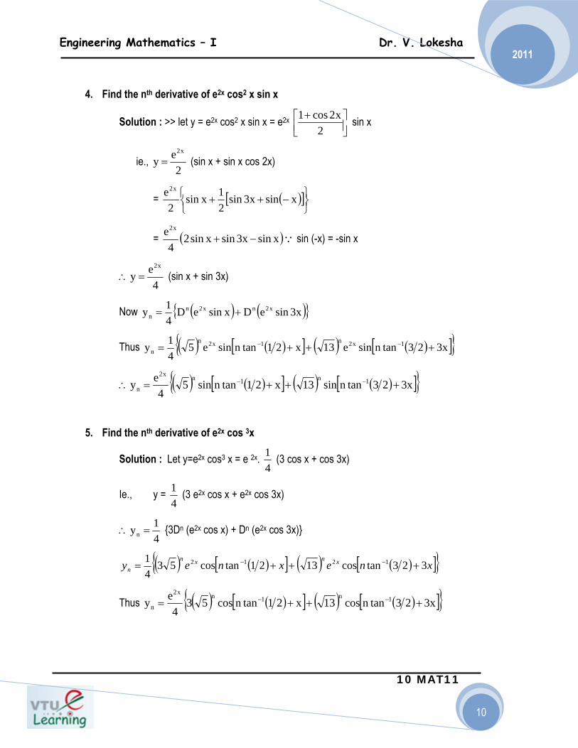
4. Find the nth derivative of e2x cos2 x sin x
Solution : >> let y = e2x cos2 x sin x = e2x ⎥⎦⎤
⎢⎣⎡ +
2x2cos1 sin x
ie., 2
eyx2
= (sin x + sin x cos 2x)
= ( )[ ]⎭⎬⎫
⎩⎨⎧ −++ xsinx3sin
21xsin
2e x2
= ( )∵xsinx3sinxsin24
e x2
−+ sin (-x) = -sin x
4ey
x2
=∴ (sin x + sin 3x)
Now ( ) ( ){ }x3sineDxsineD41y x2nx2n
n +=
Thus ( ) ( )[ ] ( ) ( )[ ]{ }x323tannsine13x21tannsine541y 1x2n1x2n
n +++= −−
( ) ( )[ ] ( ) ( )[ ]{ }x323tannsin13x21tannsin54
ey 1n1nx2
n +++=∴ −−
5. Find the nth derivative of e2x cos 3x
Solution : Let y=e2x cos3 x = e 2x. 41 (3 cos x + cos 3x)
Ie., y = 41 (3 e2x cos x + e2x cos 3x)
41yn =∴ {3Dn (e2x cos x) + Dn (e2x cos 3x)}
( ) ( )[ ] ( ) ( )[ ]{ }xnexney xnxn
n 323tancos1321tancos5341 1212 +++= −−
Thus ( ) ( )[ ] ( ) ( )[ ]{ }x323tanncos13x21tanncos534
ey 1n1nx2
n +++= −−

Engineering Mathematics – I Dr. V. Lokesha
10 MAT11
11
2011
6. Find the nth derivative of ( )( )3x21x2x2
++
Solution : ( )( )3x21x2xy
2
++= is an improper fraction because; the degree of the
numerator being 2 is equal to the degree of the denominator. Hence we must divide and rewrite the fraction.
3x8x4
x4.41
3x8x4xy 2
2
2
2
++=
++= for convenience.
4x2 +8x +3
1
2
2
38384
4
−−++
xxx
x
∴ ⎥⎦⎤
⎢⎣⎡
++−−
+=3x8x4
3x8141y 2
Ie., ⎥⎦⎤
⎢⎣⎡
+++
−=3x8x4
3x841
41y 2
The algebraic fraction involved is a proper fraction.
Now ⋅⎥⎦⎤
⎢⎣⎡
+++
−=3x8x4
3x8D410y 2
nn
Let ( )( ) 3x2B
1x2A
3x21x23x8
++
+=
+++
Multiplying by (2x + 1) (2x + 3) we have, 8x + 3 = A (2x + 3) + B (2x + 1) ................(1)
By setting 2x + 1 = 0, 2x + 3 = 0 we get x = -1/2, x = -3/2. Put x = -1/2 in (1): -1 -1 + A (2) ⇒ A = -1/2
Put x = -3/2 in (1): -9 = B (-2) ⇒ B = 9/2
∴ ⎭⎬⎫
⎩⎨⎧
⎥⎦⎤
⎢⎣⎡
++⎥⎦
⎤⎢⎣⎡
+−−=
3x21D
29
1x21D
21
41y nn
n
Engineering Mathematics – I Dr. V. Lokesha
10 MAT11
12
2011
( ) ( )( )
( )( ) ⎭
⎬⎫
⎩⎨⎧
+−
⋅++
−⋅−−= ++ 1n
nn
1n
nn
3x22!n19
1x22!n11
81
ie., ( )( ) ⎭
⎬⎫
⎩⎨⎧
++
+−
= ++
+
1n1n
n1n
n 3x29
)1x2(1
82!n1y
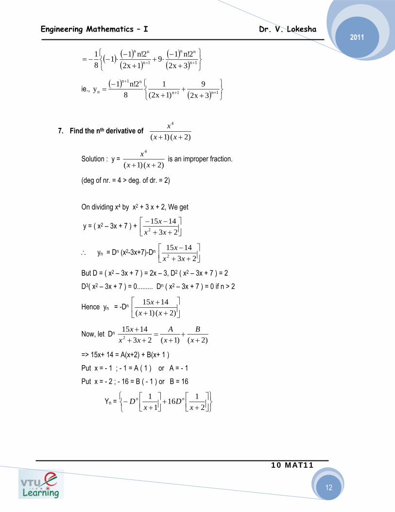
7. Find the nth derivative of )2()1(
4
++ xxx
Solution : y = )2()1(
4
++ xxx is an improper fraction.
(deg of nr. = 4 > deg. of dr. = 2) On dividing x4 by x2 + 3 x + 2, We get
y = ( x2 – 3x + 7 ) + ⎥⎦⎤
⎢⎣⎡
++−−
231415
2 xxx
∴ yn = Dn (x2-3x+7)-Dn ⎥⎦⎤
⎢⎣⎡
++−
231415
2 xxx
But D = ( x2 – 3x + 7 ) = 2x – 3, D2 ( x2 – 3x + 7 ) = 2 D3( x2 – 3x + 7 ) = 0......... Dn ( x2 – 3x + 7 ) = 0 if n > 2
Hence yn = -Dn ⎥⎦
⎤⎢⎣
⎡++
+)2()1(
1415xx
x
Now, let Dn )2()1(23
14152 +
++
=++
+x
Bx
Axx
x
=> 15x+ 14 = A(x+2) + B(x+ 1 ) Put x = - 1 ; - 1 = A ( 1 ) or A = - 1 Put x = - 2 ; - 16 = B ( - 1 ) or B = 16
Yn = ⎭⎬⎫
⎩⎨⎧
⎥⎦⎤
⎢⎣⎡
++⎥⎦
⎤⎢⎣⎡
+−
2116
11
xD
xD nn
Engineering Mathematics – I Dr. V. Lokesha
10 MAT11
13
2011
1 1
1 1
( 1) ! 1 ( 1) ! 116( 1) ( 2)
1 16( 1) ! 2( 1) ( 2)
n n n n
n n
nn n n
n nx x
y n nx x
+ +
+ +
− −= −
+ +
⎧ ⎫= − − >⎨ ⎬
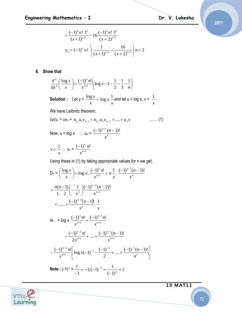
+ +⎩ ⎭ 8. Show that
⎭⎬⎫
⎩⎨⎧ −−−−
−=⎟
⎠⎞
⎜⎝⎛
+ nx
xn
xx
dxd
n
n
n
n 131
211log!)1(log
1
Solution : Let y = x
xx
x 1.loglog= and let u = log x, v =
x1
We have Leibnitz theorem,
(uv)n = uvn + vuvunvun nnCnC +++ −− ....2211 21 …… (1)
Now, u = log x ∴un = n
n
xn )!1()1( 1 −− −
xv 1
= ∴vn = 1
!)1(+
−n
n
xn
Using these in (1) by taking appropriate values for n we get,
Dn = n
n
n
n
xn
xn
xnx
xx )!1()1(.1!)1(..loglog 1
1
−−+
−=⎟
⎠⎞
⎜⎝⎛ −
+
( )
xxn
xn
xnn
n
n
n
n
1.!1)1(......
)!2()1(12.1
)1(
1
1
2
2
−−++
−−⎟⎠⎞
⎜⎝⎛−
−+
−
−
−
Ie.. = log x 1
1
1
!)1(!)1(+
−
+
−+
−n
n
n
n
xn
xn
1
1
1
2 )!1()1(....2
!)1(+
−
+
− −−++
−− n
n
n
n
xn
xn
⎥⎦
⎤⎢⎣
⎡ −−++
−−−
−−
−−−
+
−
1
121
1
2 )!1()1(....2)1()1(log!)1(
nnx
xn
n
n
Note : (-1)-1 = 1)1(
1)1(;11
12
2 =−
=−−=−
−

Engineering Mathematics – I Dr. V. Lokesha
10 MAT11
14
2011
Also nnn
nn
n 1)!1(
)!1(!
)!1(=
−−
=−
⎥⎦⎤
⎢⎣⎡ −−−−
−=⎥⎦
⎤⎢⎣⎡∴ + n
xx
nx
xdxd
n
n
n
n 1...31
211log!)1(log
1
9. If yn= Dn (xn logx) Prove that yn = n yn-1+(n-1)! and hence deduce that
yn = n ⎟⎠⎞
⎜⎝⎛ +++++
nx 1....
31
211log
Solution : yn = Dn(xn log x) = Dn-1 {D (xn log x}
= Dn-1 ⎭⎬⎫
⎩⎨⎧ + − xnx
xx nn log1. 1
= Dn-1(xn-1) + nDn-1 (xn-1 log x} ∴ yn = (n-1)! +nyn-1. This proves the first part.
Now Putting the values for n = 1, 2, 3...we get y1 = 0! + 1 y0 = 1 + log x = 1! (log x + 1 ) y2 = l! + 2y1 = l+2 (l + log x)
ie., y2 = 21og x + 3 = 2(log x + 3/2) = 2! ⎟⎠⎞
⎜⎝⎛ ++
211log x
y3 = 2! + 3y2 = 2 + 3(2 log x + 3)
ie., y3 = 61og x+ll = 6 (log x + ll/6) = 3! ⎟⎠⎞
⎜⎝⎛ +++
31
211log x
…………………………………………………………………………..
⎟⎠⎞
⎜⎝⎛ +++++=
nxnyn
1...31
211log!
10. If y = a cos (log x) + b sin ( log x), show that
x2y2 + xy1 + y = 0. Then apply Leibnitz theorem to differentiate this result n times. or If y = a cos (log x) + b sin (log x ), show that x2yn + 2 + (2n+l)xyn + l+(n2+1)yn = 0. [July-03]

Engineering Mathematics – I Dr. V. Lokesha
10 MAT11
15
2011
Solution : y = a cos (log x) + b sin (log x) Differentiate w.r.t x
∴ y1 = -a sin (log x) x1 + b cos (log x).
x1
(we avoid quotient rule to find y2) . => xy1 = - a sin (log x) + b cos (log x) Differentiating again w.r.t x we have,
xy2 + 1 y1 = - a cos (log x) + b sin ( log x) x1
or x2y2 + xy1 = - [ a cos (log x) + b sin (log x) ] = -y ∴ x2y2+xy1+y = 0 Now we have to differentiate this result n times. ie., Dn (x2y2) + Dn (xy1) + Dn (y) = 0 We have to employ Leibnitz theoreom for the first two terms. Hence we have,
⎭⎬⎫
⎩⎨⎧ −
++ −− )(.2.2.1
)1()(.2.)(. )222
12
2 yDnnyDxnyDx nnn
{ } 0)(.1.)(. 11
1 =++ −n
nn yyDnyDx
ie., {x2yn + 2 + 2n x yn + 1 + n (n – 1)yn} + {xyn+1+nyn}+yn = 0 ie., x2yn + 2 + 2n x yn + 1 + n2yn - nyn + xyn+1+nyn+yn = 0 ie., x2yn + 2 + (2n+l)xy n+l + (n2+l)yn = 0
11. If cos-1 (y/b ) = log (x/n)n, then show that
x2yn + 2 + (2n+l) xy n+l + 2n2yn = 0 Solution :By data, cos-1 (y/b) = n log (x/n) ∴log(am) = m log a
=> by = cos [n log (x/n )]
or y = b . cos [ n log (x/n)] Differentiating w.r.t x we get,
Engineering Mathematics – I Dr. V. Lokesha
10 MAT11
16
2011
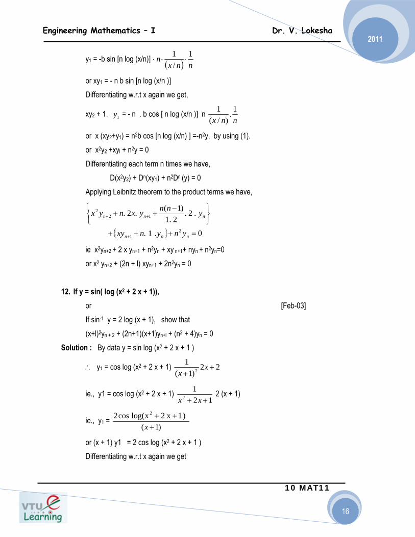
y1 = -b sin [n log (x/n)] ( ) nnxn 1
/1
⋅⋅⋅
or xy1 = - n b sin [n log (x/n )] Differentiating w.r.t x again we get,
xy2 + 1. 1y = - n . b cos [ n log (x/n )] n nnx1.
)/(1
or x (xy2+y1) = n2b cos [n log (x/n) ] =-n2y, by using (1). or x2y2 +xyl + n2y = 0 Differentiating each term n times we have,
D(x2y2) + Dn(xy1) + n2Dn (y) = 0 Applying Leibnitz theorem to the product terms we have,
{ } 0.1.
.2.2.1
)1(.2.
21
122
=+++⎭⎬⎫
⎩⎨⎧ −
++
+
++
nnn
nnn
ynynxy
ynnyxnyx
ie x2yn+2 + 2 x yn+1 + n2yn + xy n+1+ nyn + n2yn=0 or x2 yn+2 + (2n + l) xyn+1 + 2n2yn = 0
12. If y = sin( log (x2 + 2 x + 1)),
or [Feb-03] If sin-1 y = 2 log (x + 1), show that (x+l)2yn + 2 + (2n+1)(x+1)yn+l + (n2 + 4)yn = 0
Solution : By data y = sin log (x2 + 2 x + 1 )
∴ y1 = cos log (x2 + 2 x + 1) 22)1(
12 +
+x
x
ie., y1 = cos log (x2 + 2 x + 1) 12
12 ++ xx
2 (x + 1)
ie., y1 = )1(
) 1 x 2 xlog(cos2 2
+++
x
or (x + 1) y1 = 2 cos log (x2 + 2 x + 1 ) Differentiating w.r.t x again we get
Engineering Mathematics – I Dr. V. Lokesha
10 MAT11
17
2011
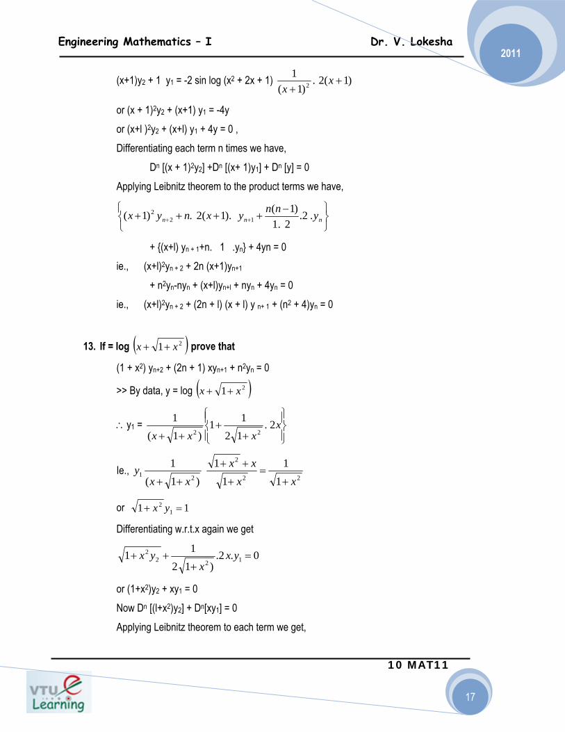
(x+1)y2 + 1 y1 = -2 sin log (x2 + 2x + 1) )1(2.)1(
12 +
+x
x
or (x + 1)2y2 + (x+1) y1 = -4y or (x+l )2y2 + (x+l) y1 + 4y = 0 , Differentiating each term n times we have,
Dn [(x + 1)2y2] +Dn [(x+ 1)y1] + Dn [y] = 0 Applying Leibnitz theorem to the product terms we have,
⎭⎬⎫
⎩⎨⎧ −
++++ ++ nnn ynnyxnyx .2.2.1
)1().1(2.)1( 122
+ {(x+l) yn + 1+n. 1 .yn} + 4yn = 0 ie., (x+l)2yn + 2 + 2n (x+1)yn+1
+ n2yn-nyn + (x+l)yn+l + nyn + 4yn = 0 ie., (x+l)2yn + 2 + (2n + l) (x + l) y n+ 1 + (n2 + 4)yn = 0
13. If = log ( )21 xx ++ prove that
(1 + x2) yn+2 + (2n + 1) xyn+1 + n2yn = 0
>> By data, y = log ( )21 xx ++
∴y1 = ⎪⎭
⎪⎬⎫
⎪⎩
⎪⎨⎧
++
++x
xxx2.
1211
)1(1
22
Ie., 22
2
211
11
1)1(
1xx
xxxx
y+
=+
++
++
or 11 12 =+ yx
Differentiating w.r.t.x again we get
0.2.)12
11 1222 =
+++ yx
xyx
or (1+x2)y2 + xy1 = 0 Now Dn [(l+x2)y2] + Dn[xy1] = 0 Applying Leibnitz theorem to each term we get,
Engineering Mathematics – I Dr. V. Lokesha
10 MAT11
18
2011
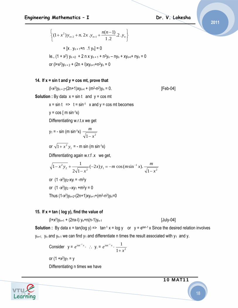
⎭⎬⎫
⎩⎨⎧ −
+++ ++ nnn ynnyxnyx .2.2.1
)1(.2.)1( 122
+ [x . yn + 1+n .1 yn] = 0 Ie., (1 + x2) yn +2 + 2 n x yn + 1 + n2yn – nyn + xyn+l+ nyn = 0 or (l+x2)yn + 2 + (2n + l)xyn+1+n2yn = 0
14. If x = sin t and y = cos mt, prove that
(l-x2)yn + 2-(2n+1)xyn+l + (m2-n2)yn = 0. [Feb-04] Solution : By data x = sin t and y = cos mt
x = sin t => t = sin-1 x and y = cos mt becomes y = cos [ m sin-1x) Differentiating w.r.t.x we get
y1 = - sin (m sin-1x) 21 x
m−
or 121 yx+ = - m sin (m sin-1x)
Differentiating again w.r.f .x we get,
2
1122
2
1).sin(cos)2(
1211
xmxmmyx
xyx
−−=−
−+− −
or (1 -x2)y2-xyl = -m2y or (1 -x2)y2 –xy1 +m2y = 0
Thus (1-x2)yn+2-(2n+1)xyn+1+(m2-n2)yn=0 15. If x = tan ( log y), find the value of (l+x2)yn+1 + (2nx-l) yn+n(n-1)yn-1 [July-04] Solution : By data x = tan(log y) => tan-1 x = log y or y = etan-1 x Since the desired relation involves yn+1, yn and yn-1 we can find y1 and differentiate n times the result associated with y1 and y.
Consider y = ⋅− xe
1tan ∴ y. = ⋅− xe
1tan21
1x+
or (1 +x2)y1 = y Differentiating n times we have
Engineering Mathematics – I Dr. V. Lokesha
10 MAT11
19
2011
Dn[(l+x2)y1]=Dn[y] Anplying Leibnitz theorem onto L.H.S, we have, {(l+x2)Dn(y1) + n .2x .Dn-1 (y1)
nn yyDnn
=−
+ − )}(.2.2.1
)1(1
2
Ie., (1+x2)yn+1+2n x yn + n (n-1) yn-1-yn=0 Or (l+x2)yn + 1 + (2nx-l)yn + n(n-l)yn-1 = 0
Engineering Mathematics – I Dr. V. Lokesha
10 MAT11
20
2011
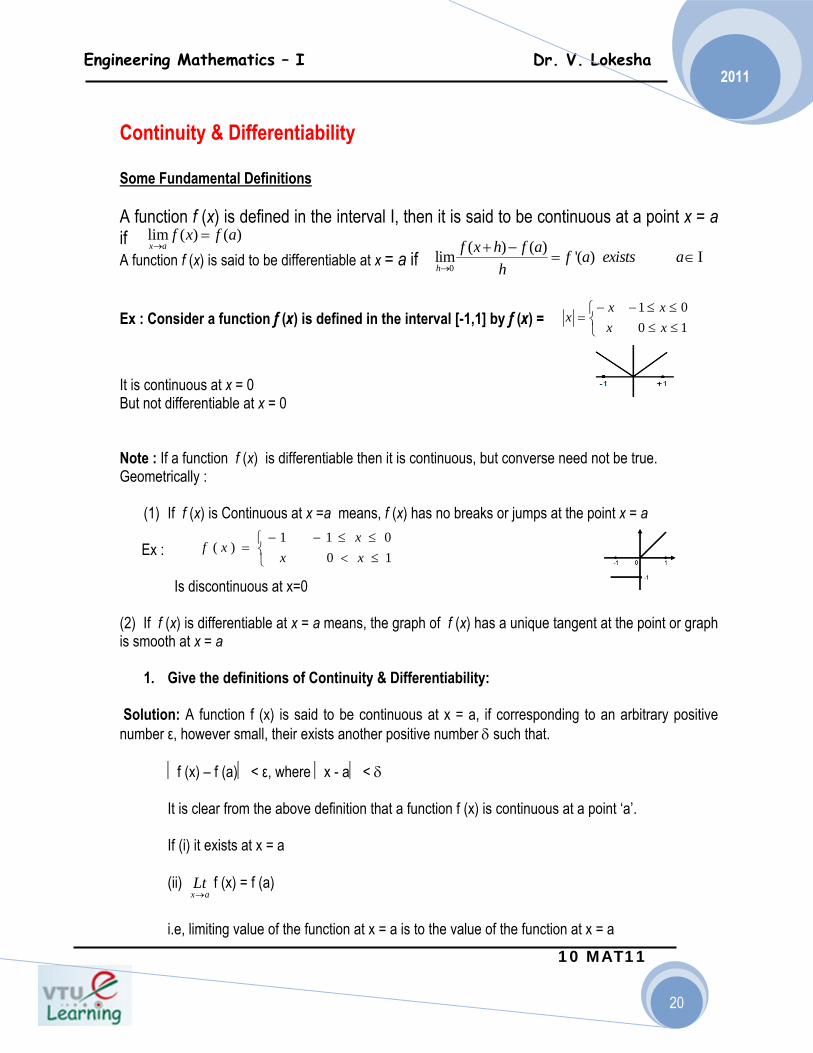
Continuity & Differentiability Some Fundamental Definitions A function f (x) is defined in the interval I, then it is said to be continuous at a point x = a if A function f (x) is said to be differentiable at x = a if Ex : Consider a function f (x) is defined in the interval [-1,1] by f (x) =
It is continuous at x = 0 But not differentiable at x = 0 Note : If a function f (x) is differentiable then it is continuous, but converse need not be true. Geometrically :
(1) If f (x) is Continuous at x =a means, f (x) has no breaks or jumps at the point x = a Ex : Is discontinuous at x=0 (2) If f (x) is differentiable at x = a means, the graph of f (x) has a unique tangent at the point or graph is smooth at x = a
1. Give the definitions of Continuity & Differentiability: Solution: A function f (x) is said to be continuous at x = a, if corresponding to an arbitrary positive number ε, however small, their exists another positive number δ such that. ⏐f (x) – f (a)⏐ < ε, where ⏐x - a⏐ < δ It is clear from the above definition that a function f (x) is continuous at a point ‘a’. If (i) it exists at x = a (ii) f (x) = f (a)
i.e, limiting value of the function at x = a is to the value of the function at x = a
axLt→
⎩⎨⎧
≤≤≤≤−−
=10 01
xxxx
x
0
( ) ( )lim '( ) Ih
f x h f a f a exists ah→
+ −= ∈
)()(lim afxfax
=→
1 1 0( )
0 1x
f xx x
− − ≤ ≤⎧= ⎨ < ≤⎩
Engineering Mathematics – I Dr. V. Lokesha
10 MAT11
21
2011
Differentiability: A function f (x) is said to be differentiable in the interval (a, b), if it is differentiable at every point in the interval. In Case [a,b] the function should posses derivatives at every point and at the end points a & b i.e., Rf1 (a) and Lf1 (a) exists.
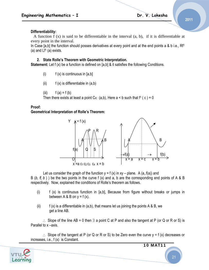
2. State Rolle’s Theorem with Geometric Interpretation. Statement: Let f (x) be a function is defined on [a,b] & it satisfies the following Conditions.
(i) f (x) is continuous in [a,b]
(ii) f (x) is differentiable in (a,b) (iii) f (a) = f (b) Then there exists at least a point C∈ (a,b), Here a < b such that f1 ( c ) = 0
Proof: Geometrical Interpretation of Rolle’s Theorem: Y y = f (x) P R A B A B f(a) Q S →f(a) → f(b) O x = a x = c x = b x =a c1 c2 c3 c4 x = b Let us consider the graph of the function y = f (x) in xy – plane. A (a,.f(a)) and B (b, f( b ) ) be the two points in the curve f (x) and a, b are the corresponding end points of A & B respectively. Now, explained the conditions of Rolle’s theorem as follows.
(i) f (x) is continuous function in [a,b], Because from figure without breaks or jumps in between A & B on y = f (x).
(ii) f (x) is a differentiable in (a,b), that means let us joining the points A & B, we
get a line AB. ∴ Slope of the line AB = 0 then ∃ a point C at P and also the tangent at P (or Q or R or S) is Parallel to x –axis. ∴ Slope of the tangent at P (or Q or R or S) to be Zero even the curve y = f (x) decreases or increases, i.e., f (x) is Constant.
Engineering Mathematics – I Dr. V. Lokesha
10 MAT11
22
2011
f1 (x) = 0 ∴f1 (c) = 0 (iii) The Slope of the line AB is equal to Zero, i.e., the line AB is parallel to x – axis. ∴ f (a) = f (b)
3. Verify Rolle’s Theorem for the function f (x) = x2 – 4x + 8 in the internal [1,3] Solution: We know that every Poly nominal is continuous and differentiable for all points and hence f (x) is continuous and differentiable in the internal [1,3]. Also f (1) = 1 – 4 + 8 = 5, f (3) = 32 – 43 + 8 = 5 Hence f (1) = f (3) Thus f (x) satisfies all the conditions of the Rolle’s Theorem. Now f1 (x) = 2x – 4 and f1 (x) = 0 ⇒ 2x – 4 = 0 or x = 2. Clearly 1 < 2 < 3. Hence there exists 2t (1,3) such that f1 (2) = 0. This shows that Rolle’s Theorem holds good for the given function f (x) in the given interval.
4. Verify Rolle’s Theorem for the function f (x) = x (x + 3) in the interval [-3, 0] Solution: Differentiating the given function W.r.t ‘x’ we get
=
∴ f1(x) exists (i.e finite) for all x and hence continuous for all x. Also f (-3) = 0, f (0) = 0 so that f (-3) = f (0) so that f (-3) = f (0). Thus f (x) satisfies all the conditions of the Rolle’s Theorem. Now, f1 (x) = 0
⇒ = 0
Solving this equation we get x = 3 or x = -2 Clearly –3 < -2 < 0. Hence there exists –2∈ (-3,0) such that f1 (-2) = 0 This proves that Rolle’s Theorem is true for the given function.
2x
e−
2221 )32(21)3()(
xxexexxxf −− ++⎟
⎠⎞
⎜⎝⎛−+=
22 )6(21 x
exx −−−−
22 )6(21 x
exx −−−−

Engineering Mathematics – I Dr. V. Lokesha
10 MAT11
23
2011
5. Verify the Rolle’s Theorem for the function Sin x in [-π, π] Solution: Let f (x) = Sin x Clearly Sinx is continuous for all x. Also f1 (x) = Cos x exists for all x in (-π, π) and f (-π) = Sin (-π) = 0; f (π) = Sin (π) = 0 so that f (-π) = f (π) Thus f (x) satisfies all the conditions of the Rolle’s Theorem . Now f1 (x) = 0 ⇒ Cos x = 0 so that
X = ±
Both these values lie in (-π,π). These exists C = ±
Such that f1 ( c ) = 0 Hence Rolle’s theorem is vertified.
6. Discuss the applicability of Rolle’s Theorem for the function f (x) = ІxІ in [-1,1]. Solution: Now f (x) = ⏐x⏐= x for 0 ≤ x ≤ 1 -x for –1 ≤ x ≤ 0 f (x) being a linear function is continuous for all x in [-1, 1]. f(x) is differentiable for all x in (-1,1) except at x = 0. Therefore Rolle’s Theorem does not hold good for the function f (x) in [-1,1]. Graph of this function is shown in figure. From which we observe that we cannot draw a tangent to the curve at any point in (-1,1) parallel to the x – axis. Y y = ⏐x⏐ x -1 0 1
2π
2π
Engineering Mathematics – I Dr. V. Lokesha
10 MAT11
24
2011
Exercise: 7. Verify Rolle’s Theorem for the following functions in the given intervals.
a) x2 – 6x + 8 in [2,4]
b) (x – a)3 (x – b)3 in [a,b]
c) log in [a,b]
8. Find whether Rolle’s Theorem is applicable to the following functions. Justify your answer.
a) f (x) = ⏐x – 1 ⏐ in [0,2]
b) f (x) = tan x in [0, π] .
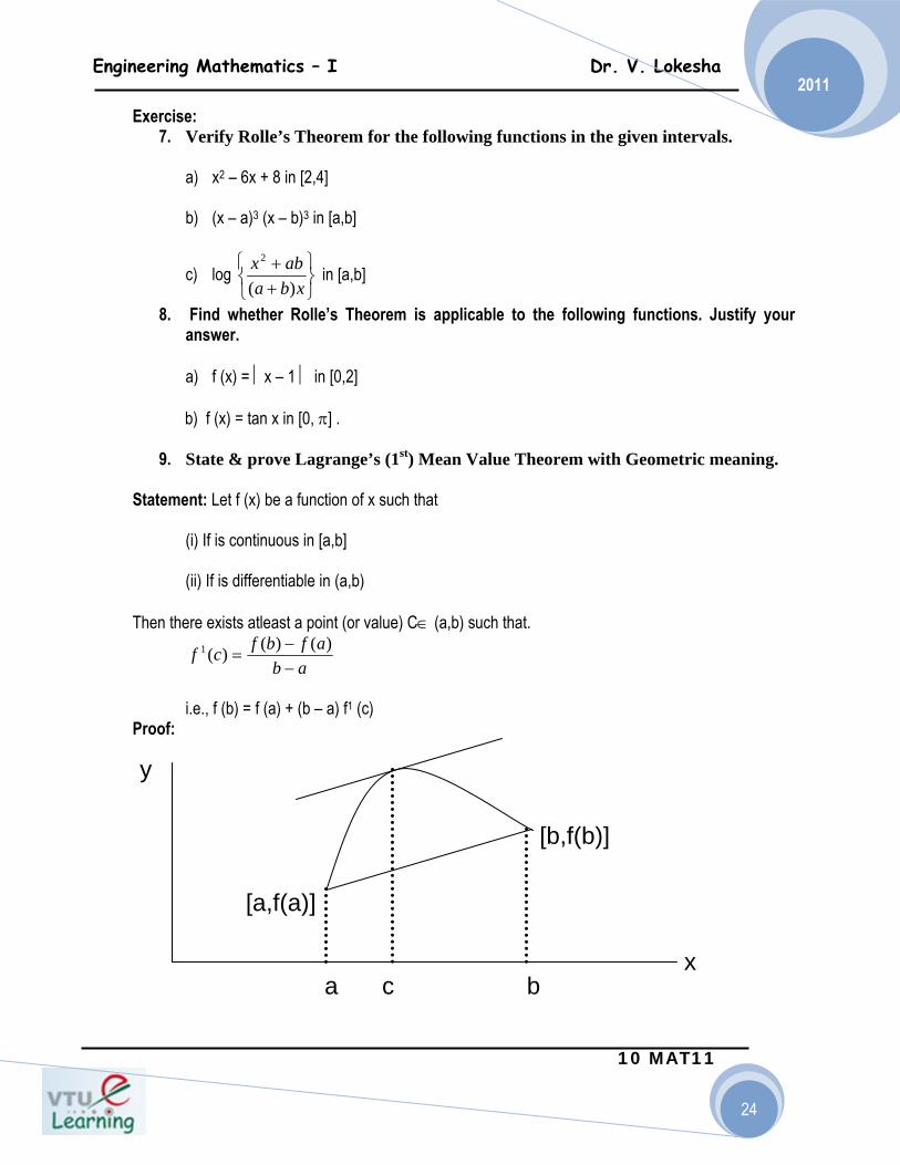
9. State & prove Lagrange’s (1st) Mean Value Theorem with Geometric meaning. Statement: Let f (x) be a function of x such that (i) If is continuous in [a,b] (ii) If is differentiable in (a,b) Then there exists atleast a point (or value) C∈ (a,b) such that.
i.e., f (b) = f (a) + (b – a) f1 (c) Proof:
⎭⎬⎫
⎩⎨⎧
++
xbaabx)(
2
abafbfcf
−−
=)()()(1
[b,f(b)]
[a,f(a)]
x
y
a c b

Engineering Mathematics – I Dr. V. Lokesha
10 MAT11
25
2011
Define a function g (x) so that g (x) = f (x) – Ax ---------- (1) Where A is a Constant to be determined. So that g (a) = g (b) Now, g (a) = f (a) – Aa G (b) = f (b) – Ab ∴ g (a) = g (b) ⇒ f (a) – Aa = f (b) – Ab.
i.e., ---------------- (2)
Now, g (x) is continuous in [a,b] as rhs of (1) is continuous in [a,b] G(x) is differentiable in (a,b) as r.h.s of (1) is differentiable in (a,b). Further g (a) = g (b), because of the choice oif A. Thus g (x) satisfies the conditions of the Rolle’s Theorem. ∴ These exists a value x = c sothat a < c < b at which g1 ( c ) = 0 ∴Differentiate (1) W.r.t ‘x’ we get g1 (x) = f 1 (x) – A ∴ g1 ( c ) = f1 ( c )- A (∵ x =c) ⇒ f 1 ( c ) - A = 0 (∵g1 ( c ) = 0) ∴f1 ( c ) = A -------------- (3) From (2) and (3) we get
(or) f (b) = f (a) + (b – a) f1 (c) For a < c < b
Corollary: Put b – a = h i.e., b = a + h and c = a + θ h Where 0 < θ < 1 Substituting in f (b) = f (a) + (b – a) f1 ( c ) ∴ f (a + h) = f (a) + h f (a + θ h), where 0 < θ < 1.
abafbfA
−−
=)()(
abafbfcf
−−
=)()()(1
Engineering Mathematics – I Dr. V. Lokesha
10 MAT11
26
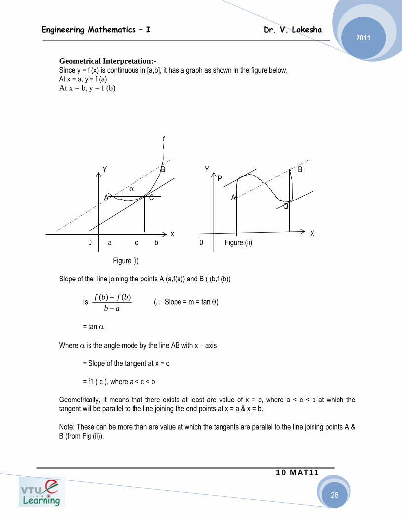
2011 Geometrical Interpretation:- Since y = f (x) is continuous in [a,b], it has a graph as shown in the figure below, At x = a, y = f (a) At x = b, y = f (b) Y B Y B P α A C A Q x X 0 a c b 0 Figure (ii) Figure (i) Slope of the line joining the points A (a,f(a)) and B ( (b,f (b))
Is (∴ Slope = m = tan θ)
= tan α Where α is the angle mode by the line AB with x – axis = Slope of the tangent at x = c = f1 ( c ), where a < c < b Geometrically, it means that there exists at least are value of x = c, where a < c < b at which the tangent will be parallel to the line joining the end points at x = a & x = b. Note: These can be more than are value at which the tangents are parallel to the line joining points A & B (from Fig (ii)).
abbfbf
−− )()(
Engineering Mathematics – I Dr. V. Lokesha
10 MAT11
27
2011
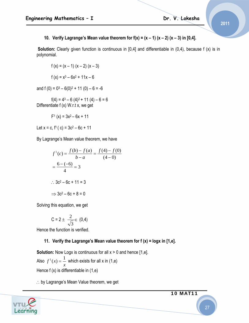
10. Verify Lagrange’s Mean value theorem for f(x) = (x – 1) (x – 2) (x – 3) in [0,4].
Solution: Clearly given function is continuous in [0,4] and differentiable in (0,4), because f (x) is in polynomial. f (x) = (x – 1) (x – 2) (x – 3) f (x) = x3 – 6x2 + 11x – 6 and f (0) = 03 – 6(0)2 + 11 (0) – 6 = -6 f(4) = 43 – 6 (4)2 + 11 (4) – 6 = 6 Differentiate f (x) W.r.t x, we get F1 (x) = 3x2 – 6x + 11 Let x = c, f1 ( c) = 3c2 – 6c + 11 By Lagrange’s Mean value theorem, we have
∴3c2 – 6c + 11 = 3 ⇒ 3c2 – 6c + 8 = 0 Solving this equation, we get
C = 2 ± ∈ (0,4)
Hence the function is verified.
11. Verify the Lagrange’s Mean value theorem for f (x) = logx in [1,e]. Solution: Now Logx is continuous for all x > 0 and hence [1,e].
Also which exists for all x in (1,e)
Hence f (x) is differentiable in (1,e) ∴by Lagrange’s Mean Value theorem, we get
)04()0()4()()()(1
−−
=−−
=ff
abafbfcf
34
)6(6=
−−=
32
xxf 1)(1 =

Engineering Mathematics – I Dr. V. Lokesha
10 MAT11
28
2011
⇒ C = e – 1 ⇒ 1 < e - < 2 < e
Since e∈ (2,3) ∴ So that c = e – 1 lies between 1 & e Hence the Theorem.
12. Find θ for f (x) = Lx2 + mx + n by Lagrange’s Mean Value theorem. Solution: f (x) = Lx2 + mx + n ∴f1 (x) = 2 Lx + m We have f (a + h) = f (a) + hf1 (a + θ h) Or f (a + h) – f (a) = hf1 (a + θ h) i.e., { (a + h)2 + m (a + h) + n} – { a2 + ma + n} = h {2 (a + θ h) + m} Comparing the Co-efficient of h2, we get
1 = 2θ ∴θ = ∈ (0,1)
Exercise:
13. Verify the Lagrange’s Mean Value theorem for f (x) = Sin2x in
14. Prove that, < tan-1 b – tan-1 a < if 0 < a < b and reduce that
15. Show that in
16. Prove that Where a < b. Hence reduce
.
ceceLogLoge 1
111
11
=−
⇒=−−
21
⎥⎦⎤
⎢⎣⎡
2,0 π
21 bab
+−
21 aab
+−
61
434tan
253
41 +<<+ − ππ
12<<
xSinx
π⎟⎠⎞
⎜⎝⎛
2,0 π
2
11
2 11 babaSinbSin
aab
−
−<−<
−
− −−
151
641
321
61 −<<− − ππ Sin
Engineering Mathematics – I Dr. V. Lokesha
10 MAT11
29
2011
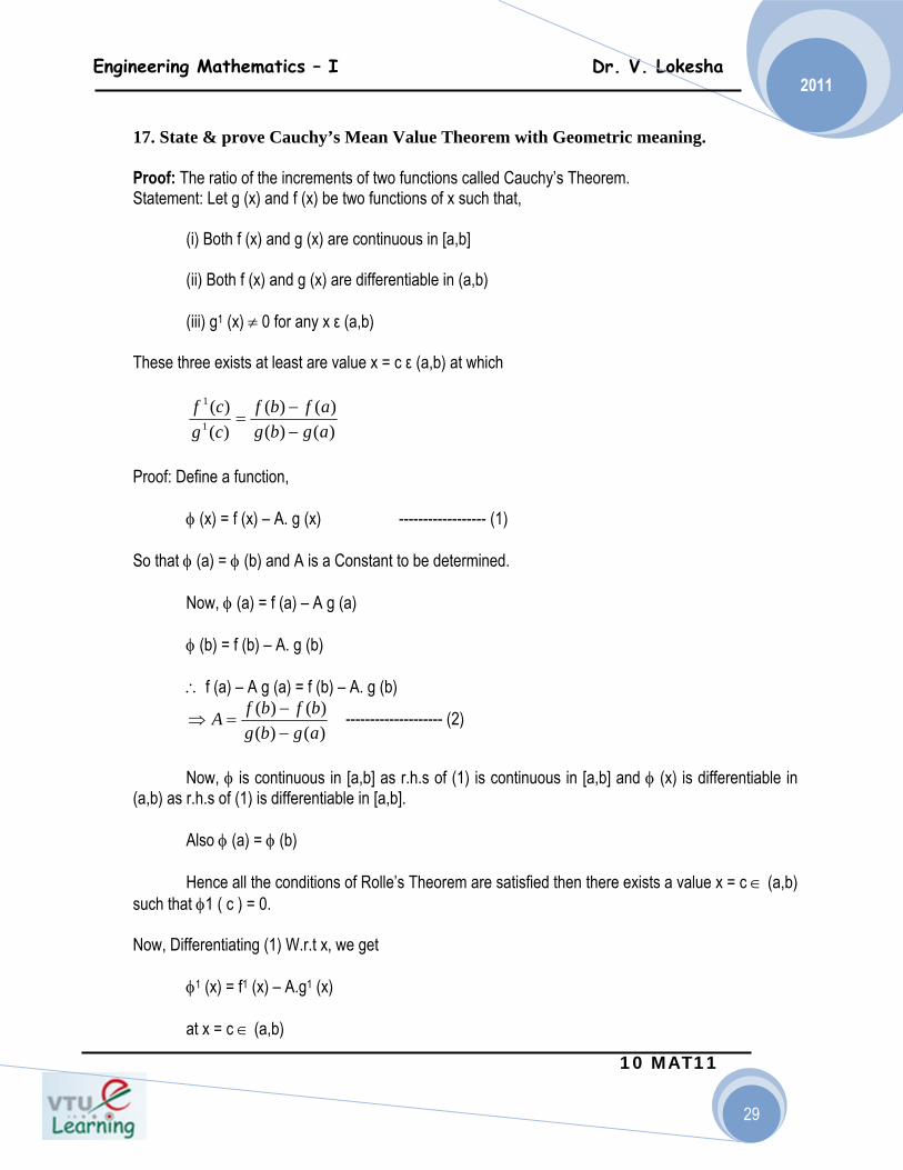
17. State & prove Cauchy’s Mean Value Theorem with Geometric meaning. Proof: The ratio of the increments of two functions called Cauchy’s Theorem. Statement: Let g (x) and f (x) be two functions of x such that, (i) Both f (x) and g (x) are continuous in [a,b] (ii) Both f (x) and g (x) are differentiable in (a,b) (iii) g1 (x) ≠ 0 for any x ε (a,b) These three exists at least are value x = c ε (a,b) at which
Proof: Define a function, φ (x) = f (x) – A. g (x) ------------------ (1) So that φ (a) = φ (b) and A is a Constant to be determined. Now, φ (a) = f (a) – A g (a) φ (b) = f (b) – A. g (b) ∴ f (a) – A g (a) = f (b) – A. g (b)
-------------------- (2)
Now, φ is continuous in [a,b] as r.h.s of (1) is continuous in [a,b] and φ (x) is differentiable in (a,b) as r.h.s of (1) is differentiable in [a,b]. Also φ (a) = φ (b) Hence all the conditions of Rolle’s Theorem are satisfied then there exists a value x = c ∈ (a,b) such that φ1 ( c ) = 0. Now, Differentiating (1) W.r.t x, we get φ1 (x) = f1 (x) – A.g1 (x) at x = c ∈ (a,b)
)()()()(
)()(
1
1
agbgafbf
cgcf
−−
=
)()()()(
agbgbfbfA
−−
=⇒

Engineering Mathematics – I Dr. V. Lokesha
10 MAT11
30
2011
∴φ1 ( c ) = f1 ( c ) – A g1 (c) 0 = f1 ( c) – A g1 ( c ) (∵ g1 (x) ≠ 0)
--------------- (3)
Substituting (3) in (2), we get
, where a < c < b
Hence the proof. 18. Verify Cauchy’s Mean Value Theorem for the function f (x) = x2 + 3, g (x) = x3 + 1 in [1,3] Solution: Here f (x) = x2 + 3, g (x) = x3 + 1 Both f (x) and g (x) are Polynomial in x. Hence they are continuous and differentiable for all x and in particular in [1,3] Now, f1 (x) = 2x, g1 (x) = 3x2 Also g 1 (x) ≠ 0 for all x ∈ (1,3) Hence f (x) and g (x) satisfy all the conditions of the cauchy’s mean value theorem. Therefore
, for some c : 1 < c < 3
i.e.,
i.e.,
Clearly C = lies between 1 and 3.
Hence Cauchy’s theorem holds good for the given function.
)()(
1
1
cgcfA =⇒
)()()()(
)()(
1
1
agbgafbf
cgcf
−−
=
)()(
)1()3()1()3(
1
1
cgcf
ggff
=−−
2326
228412
c=
−−
612
613
31
132
==⇒= Cc
612

Engineering Mathematics – I Dr. V. Lokesha
10 MAT11
31
2011
19. Verify Cauchy’s Mean Value Theorem for the functions f (x) Sin x, g (x) = Cos x in
Solution: Here f (x) = Sin x, g (x) = Cos x so that f1 (x) = Cos x ,g1 (x) = - Sinx
Clearly both f (x) and g (x) are continuous in , and differentiable in
Also g1 (x) = -Sin x ≠ 0 for all x ∈ ∴ From cauchy’s mean value theorem we obtain
for some C : 0 < C <
i.e., i.e., -1 = - Cot c (or) Cot c = 1
∴ C = , clearly C = lies between 0 and
Thus Cauchy’s Theorem is verified. Exercises: 20. Find C by Cauchy’s Mean Value Theorem for
a) f (x) = ex, g (x) = e-x in [0,1]
b) f (x) = x2, g (x) = x in [2,3] 21. Verify Cauchy’s Mean Value theorem for
a) f (x) = tan-1 x, g (x) = x in
b) f(x) = log x, g (x) = in [1,e]
⎥⎦⎤
⎢⎣⎡
2,0 π
⎥⎦⎤
⎢⎣⎡
2,0 π ( )2,0 π
( )2,0 π
)()(
)0(2
)0(2
1
1
cgcf
gg
ff=
−⎟⎠⎞
⎜⎝⎛
−⎟⎠⎞
⎜⎝⎛
π
π
2π
SincCosc−
=−−
1001
4π
4π
2π
⎥⎦
⎤⎢⎣
⎡ 1,3
1
x1
Engineering Mathematics – I Dr. V. Lokesha
10 MAT11
32
2011
Generalized Mean Value Theorem: 22. State Taylor’s Theorem and hence obtain Maclaurin’s expansion (series) Statement: If f (x) and its first (n – 1) derivatives are continuous in [a,b] and its nth derivative exists in (a,b) then
f(b) = f(a) + (b – a) f1 (a) + f11 (a) + ---------+ fn-1(a) +
Where a < c < b Remainder in Taylor’s Theorem: We have
f (x) = f (a) + (x – a) f 1 (a) + f 11 (a) + --------- + f n-1 (a) +
f n [a + (x – a) θ}
f (x) = S n (x) + R n (x)
Where R n (x) = f n [a + (x – a) θ] is called the Largrange’s form of the Remainder.
Where a = 0, R n (x) = f n (θx), 0 < θ < 1
Taylor’s and Maclaurin’s Series: We have f (x) = Sn (x) + Rn (x) ∴
If
Thus converges and its sum is f (x).
This implies that f (x) can be expressed as an infinite series.
i.e., f (x) = f (a) + (x – a) f 1 (a) + f 11 (a) + ---------- to ∞
This is called Taylor’s Series.
!2)( 2ab −
)!1()( 1
−− −
nab n
)(!
)( cfn
ab nn−
!2)( 2ax −
)!1()( 1
−− −
nax n
nax n
∠− )(
!)(
nax n−
!nxn
)()]()([ xRLimxSxfLim nnnn ∞→∞→=−
)()(0)( xSLimxthenfxRLim nnnn ∞→∞→=
)(xSLim nn ∞→
!2)( 2ax −
Engineering Mathematics – I Dr. V. Lokesha
10 MAT11
33
2011
Putting a = 0, in the above series, we get
F (x) = f (0) + x f 1 (0) + f 11 (0) + --------- to ∞
This is called Maclaurin’s Series. This can also denoted as
Y = y (0) + x y 1 (0) + y 2 (0) + -------- + y n (0) ---------- to ∞
Where y = f (x), y1 = f 1 (x), -------------- y n = f n (x) 23. By using Taylor’s Theorem expand the function e x in ascending powers of (x – 1) Solution: The Taylor’s Theorem for the function f (x) is ascending powers of (x – a) is
f (x) = f (a) + (x – a) f 1 (a) + f 11 (a) + ------------ (1)
Here f (x) = e x and a = 1 f 1 (x) = e x ⇒ f 1 (a) = e f 11 (x) = e x ⇒ f 11 (a) = e ∴ (1) becomes
e x = e + (x – 1) e + e + -------------
= e { 1 + (x – 1) + + --------}
24. By using Taylor’s Theorem expand log sinx in ascending powers of (x – 3) Solution: f (x) = Log Sin x, a = 3 and f (3) = log sin3
Now f 1 (x) = = Cotx, f 1 (3) = Cot3
f 11 (x) = - Cosec 2x, f 11 (3) = - Cosec 23
f 111 (x) = - 2Cosecx (-Cosecx Cotx) = 2Cosec 3x Cotx ∴ f 111 (3) = 2Cosec 33 Cot3
∴ f (x) = f (a) + (x – a) f 1 (a) + f 11 (a) + f 111 (a) + ------------
∴Log Sinx = f (3) + (x – 3) f 1(3) + f 11 (3) + f 111 (3) + -----------
= logsin3 + (x – 3) Cot3 + (-Cosec23) + 2 Cosec 33Cot3 + ---
!2)( 2x
!2)( 2x
!)(
nx n
2)( 2
∠− ax
2)1( 2−x
2)1( 2−x
SinxCosx
!2)( 2ax −
!3)( 3ax −
!2)3( 2−x
!3)3( 3−x
!2)3( 2−x
!3)3( 3−x
Engineering Mathematics – I Dr. V. Lokesha
10 MAT11
34
2011
Exercise:
25. Expand Sinx is ascending powers of
26. Express tan –1 x in powers of (x – 1) up to the term containing (x – 1) 3 27. Apply Taylor’s Theorem to prove
e x + h = e x
Problems on Maclaurin’s Expansion:
28. Expand the log (1 + x) as a power series by using Maclaurin’s theorem. Solution: Here f (x) = log (1 + x), Hence f (0) = log 1 = 0 We know that
= , n = 1,2,---------
Hence f n (0) = (-1) n-1 (n – 1) ! f 1 (0) = 1, f 11 (0) = -1, f 111 (0) = 3!, f 1v (0) = - 3! Substituting these values in
f (x) = f (0) + x f 1 (0) + f 11 (0) + -------- + f n (0) + ------------
∴ log (1+x) = 0 + x . 1 + (-1) + 2! + - 3! + ---------------
= x - + - + ---------
This series is called Logarithmic Series.
⎟⎠⎞
⎜⎝⎛ −
2πx
⎥⎦
⎤⎢⎣
⎡−−−−−−−−−++++
!3!21
32 hhh
{ }⎭⎬⎫
⎩⎨⎧
+=+= −
−
xdxdx
dxdxf n
n
n
nn
11)1log()( 1
1
n
n
nn)1(
)!1()1( 1
+−− −
!2
2x!n
xn
!2
2x!3
3x!4
4x
2
2x3
3x4
4x

Engineering Mathematics – I Dr. V. Lokesha
10 MAT11
35
2011
29. Expand tan –1 x by using Macluarin’s Theorem up to the term containing x 5 Solution: let y = tan –1 x, Hence y (0) = 0
We find that y 1 = which gives y 1 (0) = 1
Further y 1 (1 + x 2) = 1, Differentiating we get Y 1 . 2x + (1 + x 2) y 2 = 0 (or) (1 + x2) y 2 + 2xy 1 = 0 Hence y 2 (0) = 0 Taking n th derivative an both sides by using Leibniz’s Theorem, we get
(1 + x 2) y n + 2 + n . 2xy n +1 + . 2. y n + 2xy n – 1 + n.2.y n = 0
i.e., (1 + x 2) y n + 2 + 2 (n +1) x y n + 1 + n (n + 1) y n = 0 Substituting x = 0, we get, y n + 2 (0) = -n (n + 1) y n (0) For n = 1, we get y 3 (0) = - 2y 1 (0) = - 2 For n = 2, we get y 4 (0) = - 2 .3.y 2 (0) = 0 For n = 3, we get y 5 (0) = - 3.4.y 3 (0) = 24 Using the formula
Y = y (0) + x y 1 (0) + y 2 (0) + y 3 (0) + ---------
We get tan –1 x = x - + - -------------
Exercise: 30. Using Maclaurin’s Theorem prove the following:
a) Secx = 1 + + + --------
b) Sin –1 x = x + + + --------------
c) e x Cos x = 1 + x - + ---------------
d) Expand e ax Cos bx by Maclaurin’s Theorem as far as the term containing x 3
211x+
2.1)1( −nn
!2
2x!3
3x
3
3x5
5x
!2
2x!4
5 4x
6
3x40
3 5x
3
3x
Engineering Mathematics – I Dr. V. Lokesha
10 MAT11
36
2011
Exercise : Verify Rolle’s Theorem for
(i) in ,
(ii) in
(iii) in .
Exercise : Verify the Lagrange’s Mean Value Theorem for
(i) in
(ii) in
Exercise : Verify the Cauchy’s Mean Value Theorem for
(i) and in
(ii) and in
(iii) and in
)cos(sin)( xxexf x −= ⎥⎦⎤
⎢⎣⎡
45,
4ππ
2/)2()( xexxxf −= [ ]2,0
2sin 2( ) x
xf xe
= ⎥⎦⎤
⎢⎣⎡
45,
4ππ
( ) ( 1)( 2)f x x x x= − −10,2
⎡ ⎤⎢ ⎥⎣ ⎦
1( )f x Tan x−= [ ]0,1
( )f x x=1( )g xx
= 1 ,14
⎡ ⎤⎢ ⎥⎣ ⎦
21( )f xx
=1( )g xx
= [ ],a b
( )f x Sin x= ( )g x Cos x= [ ],a b

Engineering Mathematics – I Dr. V. Lokesha
10 MAT11
37
2011
UNIT – II
DIFFERENTIAL CALCULUS-II
Give different types of Indeterminate Forms. If f (x) and g (x) be two functions such that and both exists, then
If = 0 and = 0 then
Which do not have any definite value, such an expression is called
indeterminate form. The other indeterminate forms are , 00, ∞0 and 1 ∞
1. State & prove L’ Hospital’s Theorem (rule) for Indeterminate Forms.
L’Hospital rule is applicable when the given expression is of the form or
Statement: Let f (x) and g (x) be two functions such that (1) = 0 and = 0
(2) f1 (a) and g1 (a) exist and g1 (a) ≠ 0
Then
Proof: Now , which takes the indeterminate form . Hence applying the
L’ Hospitals theorem, we get
)(xfLimax→
)(xgLimax→
)(
)(
)()(
xgLim
xfLim
xgxfLim
ax
ax
ax→
→
→=
)(xfLimax→
)(xgLimax→
00
)()(
=→ xg
xfLimax
∞−∞∞×∞∞ ,0,
00
∞∞
)(xfLimax→
)(xgLimax→
)(
)(
)()(
1
1
xgLim
xfLim
xgxfLim
ax
ax
ax→
→
→=
⎥⎥⎥
⎦
⎤
⎢⎢⎢
⎣
⎡=
→→)(
1
1
)()(
xf
xgLimxgxfLim
axax 00

Engineering Mathematics – I Dr. V. Lokesha
10 MAT11
38
2011
If then
1
i.e
If = 0 or ∞ the above theorem still holds good.
2. Evaluate form
Solution: Apply L’Hospital rule, we get
= 1
3. Evaluate
Solution: = form
Apply L’ Hospital rule
=
2
1
1
2
1
2
1
)()(
)()(
)]([)(
)]([)(
)()(
⎥⎦
⎤⎢⎣
⎡=
−
−
=→→→ xg
xfxfxgLim
xfxf
xgxg
LimxgxfLim
axaxax
2
1
1
)()(
)()(
⎥⎦
⎤⎢⎣
⎡⎥⎦
⎤⎢⎣
⎡=
→→ xgxfLim
xfxgLim
axax
∞≠≠→
andxgxfLim
ax0
)()(
⎥⎦
⎤⎢⎣
⎡⎥⎦
⎤⎢⎣
⎡=
→→ )()(
)()(
1
1
xgxfLim
xfxgLim
axax
)()(
)()(
1
1
xgxfLim
xgxfLim
axax →→=
)()(
xgxfLim
ax→
00
=→ x
SinxLimax
11
11==
→
θCosCosxLimax
1=∴→ x
SinxLimax
CotxSinxLim
ax
log→
CotxSinxLim
ax
log→ ∞
∞−=
∞=
0log0
0logCot
Sin
xCotxxCoCoxCosceLim
ax secsec2
2
−−
→
Engineering Mathematics – I Dr. V. Lokesha
10 MAT11
39
2011
Exercise: 1
Evaluate
a)
b)
c)
d )
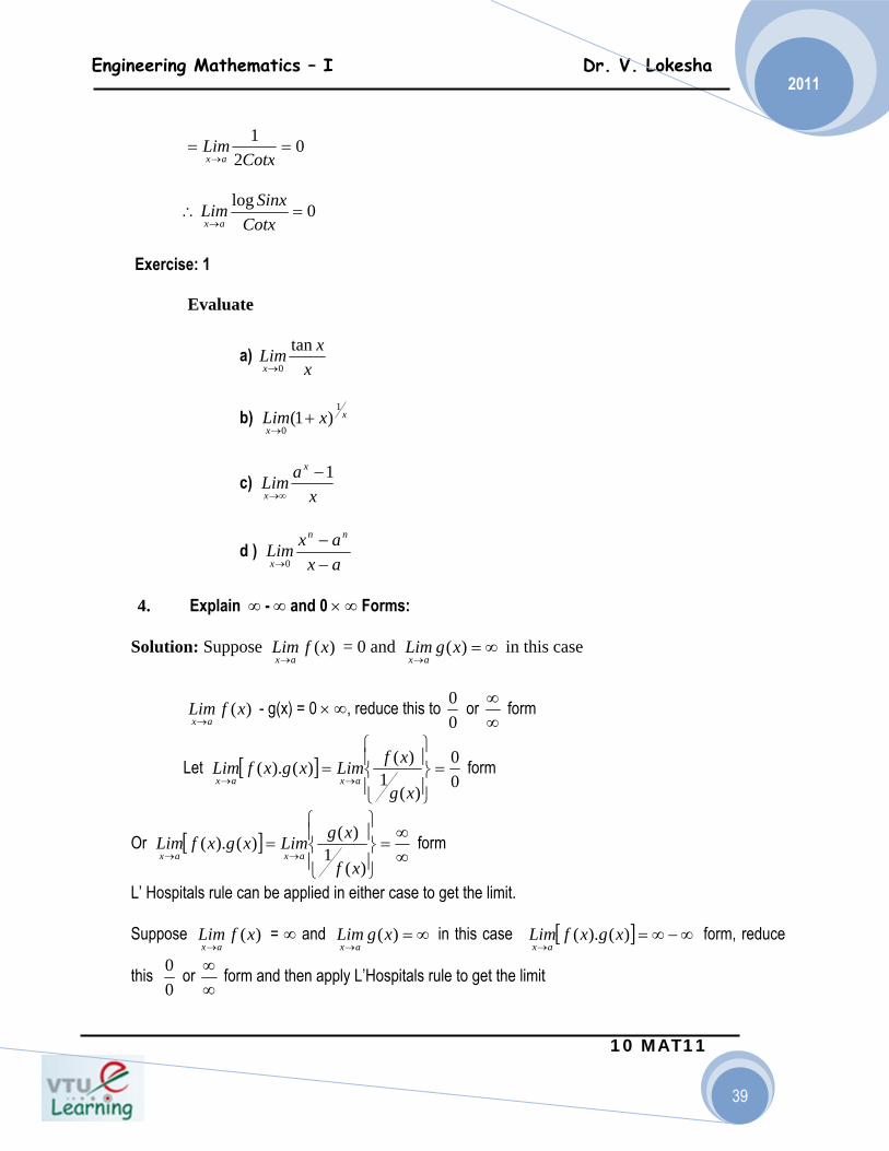
4. Explain ∞ - ∞ and 0 × ∞ Forms:
Solution: Suppose = 0 and in this case
- g(x) = 0 × ∞, reduce this to or form
Let form
Or form
L’ Hospitals rule can be applied in either case to get the limit. Suppose = ∞ and in this case form, reduce
this or form and then apply L’Hospitals rule to get the limit
02
1==
→ CotxLim
ax
0log=∴
→ CotxSinxLim
ax
xxLim
x
tan0→
xx
xLim1
0)1( +
→
xaLim
x
x
1−∞→
axaxLim
nn
x −−
→0
)(xfLimax→
∞=→
)(xgLimax
)(xfLimax→ 0
0∞∞
[ ]00
)(1
)()().( =⎪⎭
⎪⎬⎫
⎪⎩
⎪⎨⎧
=→→
xg
xfLimxgxfLimaxax
[ ]∞∞
=⎪⎭
⎪⎬⎫
⎪⎩
⎪⎨⎧
=→→
)(1
)()().(xf
xgLimxgxfLimaxax
)(xfLimax→
∞=→
)(xgLimax
[ ] ∞−∞=→
)().( xgxfLimax
00
∞∞

Engineering Mathematics – I Dr. V. Lokesha
10 MAT11
40
2011
5. Evaluate
Solution: Given = ∞ - ∞ form
∴ Required limit = form
Apply L’Hospital rule.
=
6. Evaluate
Solution: Given limit is ∞ - ∞ form at x = 0. Hence we have
Required limit =
= form
Apply L’ Hospital’s rule
=
= form
Apply L’ Hospitals rule
⎭⎬⎫
⎩⎨⎧ +
−→ 20
)1log(1x
xx
Limx
⎭⎬⎫
⎩⎨⎧ +
−→ 20
)1log(1x
xx
Limx
001log(
20=
⎭⎬⎫
⎩⎨⎧ +−
→ xxxLim
x
xxLim
x 21
11
0
+−
→
21
)1(21
21
00=
+=+=
→→ xLim
xx
x
Limxx
⎭⎬⎫
⎩⎨⎧ −
→Cotx
xLimx
10
⎭⎬⎫
⎩⎨⎧ −
→ SinxCosx
xLimx
10
⎟⎠⎞
⎜⎝⎛=⎟
⎠⎞
⎜⎝⎛ −
→ 00
0 xSinxxCosxSinxLim
x
SinxxCosxxSinxCosxCosxLim
x ++−
→0
⎟⎠⎞
⎜⎝⎛=
+→ 00
0 SinxxCosxxSinxLim
x
Engineering Mathematics – I Dr. V. Lokesha
10 MAT11
41
2011
=
=
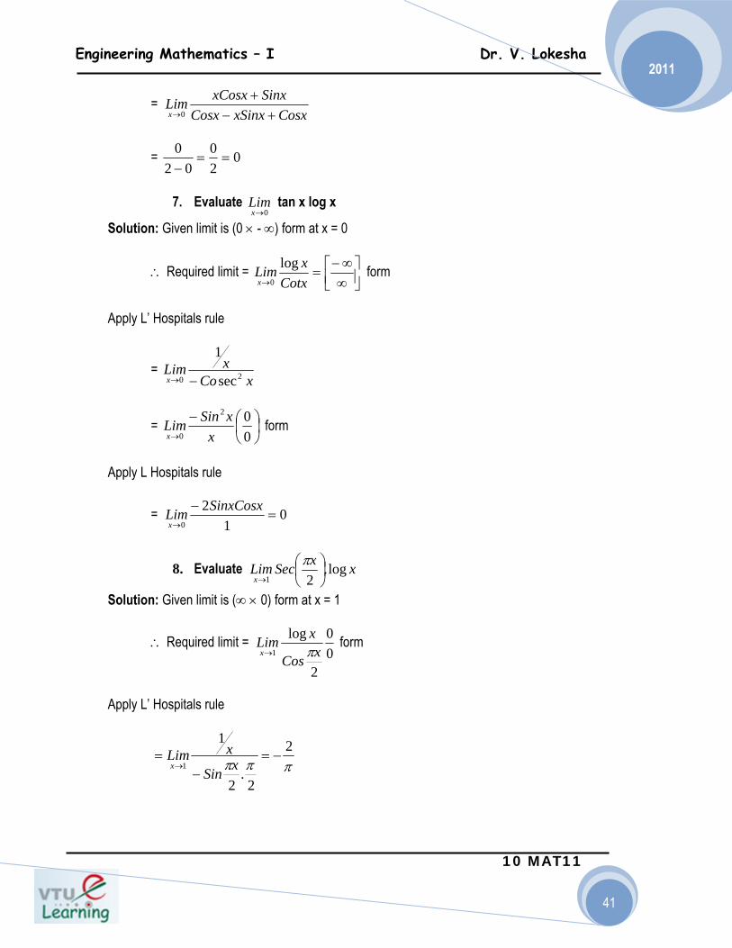
7. Evaluate tan x log x
Solution: Given limit is (0 × - ∞) form at x = 0
∴ Required limit = form
Apply L’ Hospitals rule
=
= form
Apply L Hospitals rule
=
8. Evaluate
Solution: Given limit is (∞ × 0) form at x = 1
∴ Required limit = form
Apply L’ Hospitals rule
CosxxSinxCosxSinxxCosxLim
x +−+
→0
020
020
==−
0→xLim
⎥⎦⎤
⎢⎣⎡
∞∞−
=→ Cotx
xLimx
log0
xCoxLim
x 20 sec
1
−→
⎟⎠⎞
⎜⎝⎛−
→ 002
0 xxSinLim
x
01
20
=−
→
SinxCosxLimx
xxSecLimx
log.21
⎟⎠⎞
⎜⎝⎛
→
π
00
2
log1 xCos
xLimx π→
πππ2
2.
2
1
1−=
−=
→ xSin
xLimx
Engineering Mathematics – I Dr. V. Lokesha
10 MAT11
42
2011
Exercise: 2
Evaluate
a)
b)
c)
d)
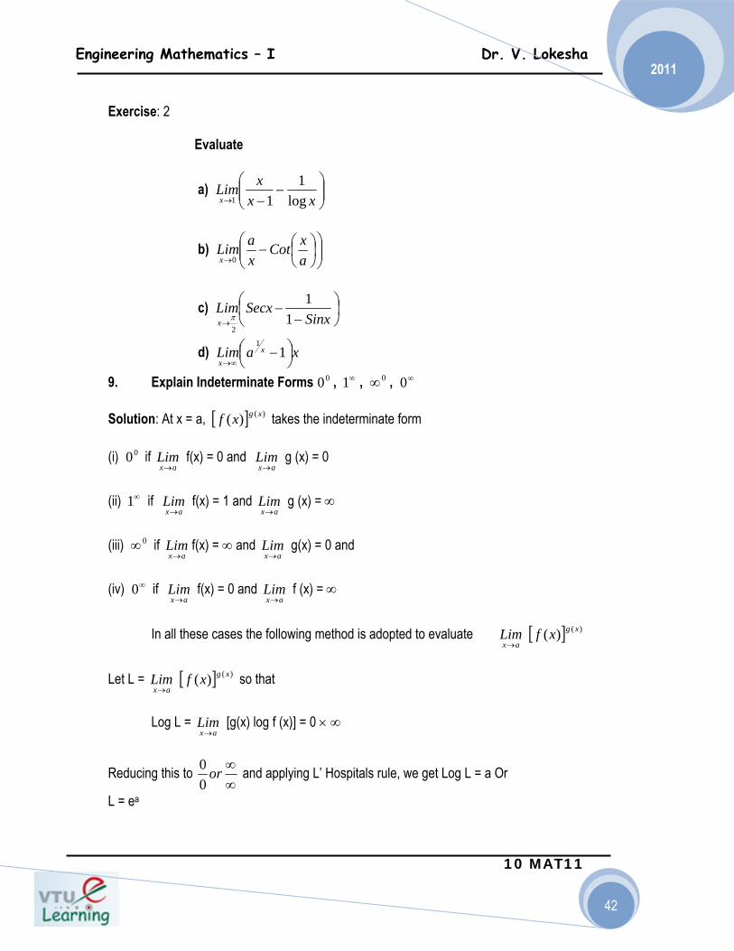
9. Explain Indeterminate Forms , , , Solution: At x = a, takes the indeterminate form (i) if f(x) = 0 and g (x) = 0 (ii) if f(x) = 1 and g (x) = ∞
(iii) if f(x) = ∞ and g(x) = 0 and
(iv) if f(x) = 0 and f (x) = ∞
In all these cases the following method is adopted to evaluate
Let L = so that
Log L = [g(x) log f (x)] = 0 × ∞
Reducing this to and applying L’ Hospitals rule, we get Log L = a Or
L = ea
⎟⎟⎠
⎞⎜⎜⎝
⎛−
−→ xxxLim
x log1
11
⎟⎟⎠
⎞⎜⎜⎝
⎛⎟⎠⎞
⎜⎝⎛−
→ axCot
xaLim
x 0
⎟⎠⎞
⎜⎝⎛
−−
→ SinxSecxLim
x 11
2π
xaLim xx
⎟⎠⎞⎜
⎝⎛ −
∞→1
1
00 ∞1 0∞ ∞0
[ ] )()( xgxf
00ax
Lim→ ax
Lim→
∞1ax
Lim→ ax
Lim→
0∞ax
Lim→ ax
Lim→
∞0ax
Lim→ ax
Lim→
axLim
→[ ] )()( xgxf
axLim
→[ ] )()( xgxf
axLim
→
∞∞or
00
Engineering Mathematics – I Dr. V. Lokesha
10 MAT11
43
2011
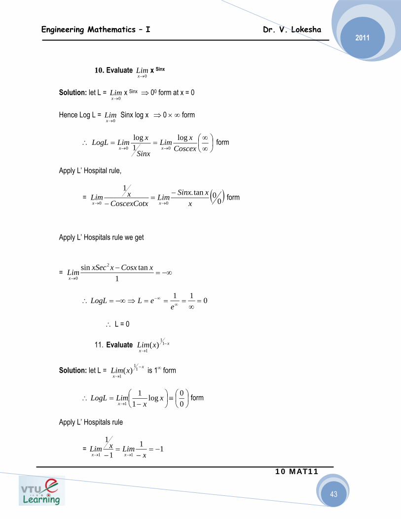
10. Evaluate x Sinx
Solution: let L = x Sinx ⇒ 00 form at x = 0
Hence Log L = Sinx log x ⇒ 0 × ∞ form
∴ form
Apply L’ Hospital rule,
= form
Apply L’ Hospitals rule we get
=
∴ L = 0
11. Evaluate
Solution: let L = is 1∞ form
form
Apply L’ Hospitals rule
=
0→xLim
0→xLim
0→xLim
⎟⎠⎞
⎜⎝⎛
∞∞
==→→ Coscex
xLimSinx
xLimLogLxx
log1log
00
( )00tan.1
00 xxSinxLim
CoscexCotxxLim
xx
−=
− →→
−∞=−
→ 1tansin 2
0
xCosxxxSecLimx
011=
∞===⇒−∞=∴ ∞
∞−
eeLLogL
xx
xLim −
→
11
1)(
x
xxLim −
→
11
1)(
⎟⎠⎞
⎜⎝⎛≡⎟
⎠⎞
⎜⎝⎛
−=∴
→ 00log
11
1x
xLimLogLx
111
1
11−=
−=
− →→ xLimxLimxx

Engineering Mathematics – I Dr. V. Lokesha
10 MAT11
44
2011
∴ Log L = -1
⇒ L =
12. Evaluate
Solution: let L = form
form
form
Apply L’ Hospitals rule
=
form
Apply L’ Hospital rule, we get
Log L =
ee 11 =−
21
0
tan x
x xxLim ⎟
⎠⎞
⎜⎝⎛
→
∞
→≡⎟
⎠⎞
⎜⎝⎛ 1tan 2
1
0
x
x xxLim
)0(tanlog120
×∞≡⎭⎬⎫
⎩⎨⎧
⎟⎠⎞
⎜⎝⎛=∴
→ xx
xLimLogLx
( )⎟⎠⎞
⎜⎝⎛≡
⎪⎭
⎪⎬⎫
⎪⎩
⎪⎨⎧
=∴→ 0
0tanlog20 x
xx
LimLogLx
⎪⎪⎭
⎪⎪⎬
⎫
⎪⎪⎩
⎪⎪⎨
⎧ −
→ xx
xxxSec
xx
Limx 2
tan
tan1 2
2
0
⎟⎠⎞
⎜⎝⎛=⎥
⎦
⎤⎢⎣
⎡ −=
→ 00tan
21
3
2
0 xxxxSecLimLogL
x
2
222
0 3tan2
21
xxSecxxxSecxSecLim
x
−+=
→
⎟⎠⎞
⎜⎝⎛=
→ xxxSecLim
x
tan)(31 2
0
31
31
eL =∴

Engineering Mathematics – I Dr. V. Lokesha
10 MAT11
45
2011
Exercise: 3 Evaluate the following limits.
a) b)
c) d)
Evaluate the following limits.
Cotx
xSecxLim )(
0→
⎟⎠⎞
⎜⎝⎛
→⎟⎠⎞
⎜⎝⎛ −
ax
ax axLim
2tan
2π
xexLim
x
x
−+→
1
0
)1( 2)(0
xx
CosaxLim∞
→
3
30 0
2 log(1 ) log(1 )( ) lim ( ) limsin sin
x x
x x
e e x xi iix x x
−
→ →
− − + +
20 22
1 sin cos log(1 ) log sin( ) lim ( ) limtan ( )
2x x
x x x xiii ivx x x
π π→ →
+ − + −
−
1
2 202
cosh log(1 ) 1 sin sin( ) lim ( ) limx x
x x x x xv vix xπ
−
→ →
+ − − +
2 2
0
(1 )( ) limlog(1 )
x
x
e xviix x→
− ++
( )0
( ) lim 2 cot( ) ( ) lim cos cotx a x
xi x a ii ecx xa→ →
⎛ ⎞− − −⎜ ⎟⎝ ⎠
220
2
1( ) lim tan sec ( ) lim cot2 xx
iii x x x iv xxπ
π→→
⎡ ⎤ ⎛ ⎞− −⎜ ⎟⎢ ⎥⎣ ⎦ ⎝ ⎠
[ ]202
1 1( ) lim ( ) lim 2 tan sectanx x
v vi x x xx x x π
π→ →
⎡ ⎤− −⎢ ⎥⎣ ⎦
22
1
0 0
1 cos( ) lim(cos ) ( ) lim2
b xx
x x
xi ax ii→ →
⎛ ⎞+⎜ ⎟⎝ ⎠
Engineering Mathematics – I Dr. V. Lokesha
10 MAT11
46
2011
Evaluate the following limits.
21
12 log(1 )
1 0
sin( ) lim(1 ) ( ) limx
x
x x
xiii x ivx
−
→ →
⎛ ⎞− ⎜ ⎟
⎝ ⎠
( )cottan
0 0( ) lim(sin ) ( ) lim 1 sin xx
x xv x iv x
→ →+
( )2 tan 2cos
04
( ) lim(cos ) ( ) lim tan xec x
x xvii x viii x
π→ →
1
0
1( ) lim( ) ( ) lim1 3
x x x xx
x x
ax a b cix xax→∞ →
⎛ ⎞+ + +⎜ ⎟− ⎝ ⎠
22
1
0 0
1 cos( ) lim(cos ) ( ) lim2
b xx
x x
xi ax ii→ →
⎛ ⎞+⎜ ⎟⎝ ⎠
21
12 log(1 )
1 0
sin( ) lim(1 ) ( ) limx
x
x x
xiii x ivx
−
→ →
⎛ ⎞− ⎜ ⎟
⎝ ⎠
( )cottan
0 0( ) lim(sin ) ( ) lim 1 sin xx
x xv x iv x
→ →+
( )2 tan 2cos
04
( ) lim(cos ) ( ) lim tan xec x
x xvii x viii x
π→ →
1
0
1( ) lim( ) ( ) lim1 3
x x x xx
x x
ax a b cix xax→∞ →
⎛ ⎞+ + +⎜ ⎟− ⎝ ⎠

Engineering Mathematics – I Dr. V. Lokesha
10 MAT11
47
2011
Polar Curves If we traverse in a hill section where the road is not straight, we often see caution boards hairpin bend ahead, sharp bend ahead etc. This gives an indication of the difference in the amount of bending of a road at various points which is the curvature at various points. In this chapter we discuss about the curvature, radius of curvature etc. Consider a point P in the xy-Plane.
r = length of OP= radial distance θ = Polar angle ( r, θ)→ Polar co-ordinates
Let r = f (θ) be the polar curve x = r Cos θ y = r Sin θ
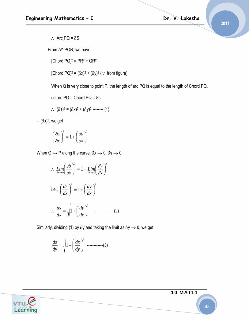
Relation (1) enables us to find the polar co-ordinates ( r, θ) when the Cartesian co-ordinates ( x, y) are known. Expression for arc length in Cartesian form. Proof: Let P (x,y) and Q (x + δx, Y + δy) be two neighboring points on the graph of the function y = f (x). So that they are at length S and S + δs measured from a fixed point A on the curve. Y = f (x) Q T (Tangent) δs δy A δx N O δx X
From figure, ,
∠TPR = ψ and PR =δx, RQ = δy
SPQ δ=∩
SAP =∩
( )2 2 1, tan (1)yr x y xθ − −−−−−−= + =
Engineering Mathematics – I Dr. V. Lokesha
10 MAT11
48
2011
∴ Arc PQ = δS From ∆le PQR, we have [Chord PQ]2 = PR2 + QR2 [Chord PQ]2 = (δx)2 + (δy)2 (∵ from figure) When Q is very close to point P, the length of arc PQ is equal to the length of Chord PQ. i.e arc PQ = Chord PQ = δs ∴ (δs)2 = (δx)2 + (δy)2 -------- (1) ÷ (δx)2, we get
When Q → P along the curve, δx → 0, δs → 0
i.e.,
∴ --------------(2)
Similarly, dividing (1) by δy and taking the limit as δy → 0, we get
------------(3)
22
1 ⎟⎠⎞
⎜⎝⎛+=⎟
⎠⎞
⎜⎝⎛
xy
xs
δδ
δδ
2
0
2
01 ⎟
⎠⎞
⎜⎝⎛+=⎟
⎠⎞
⎜⎝⎛∴
→→ xyLim
xsLim
xx δδ
δδ
δδ
22
1 ⎟⎠⎞
⎜⎝⎛+=⎟
⎠⎞
⎜⎝⎛
dxdy
dxds
2
1 ⎟⎠⎞
⎜⎝⎛+=
dxdy
dxds
2
1 ⎟⎟⎠
⎞⎜⎜⎝
⎛+=
dydx
dyds
Engineering Mathematics – I Dr. V. Lokesha
10 MAT11
49
2011
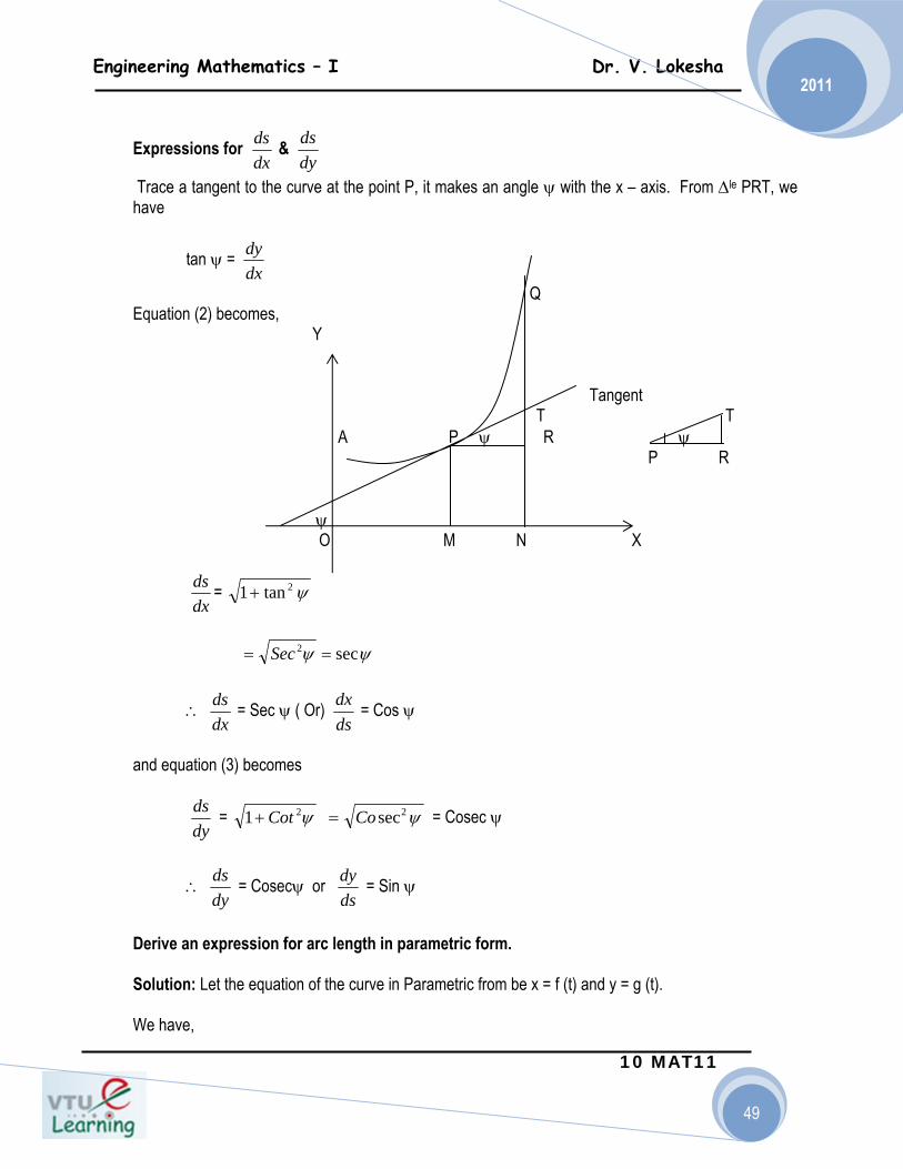
Expressions for &
Trace a tangent to the curve at the point P, it makes an angle ψ with the x – axis. From ∆le PRT, we have
tan ψ =
Q Equation (2) becomes, Y Tangent T T A P ψ R ψ P R ψ O M N X
=
∴ = Sec ψ ( Or) = Cos ψ
and equation (3) becomes
= = Cosec ψ
∴ = Cosecψ or = Sin ψ
Derive an expression for arc length in parametric form. Solution: Let the equation of the curve in Parametric from be x = f (t) and y = g (t). We have,
dxds
dyds
dxdy
dxds ψ2tan1+
ψψ sec2 == Sec
dxds
dsdx
dyds ψ21 Cot+ ψ2secCo=
dyds
dsdy

Engineering Mathematics – I Dr. V. Lokesha
10 MAT11
50
2011
(δs)2 = (δx)2 + (δy)2 ÷ by (δt)2, we get
Taking the limit as δt → 0 on both sides, we get
(Or) ------------ (4)
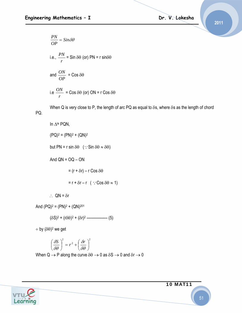
Derive an expression for arc length in Cartesian form. Solution: Let P (r,θ) and Q (r + δr, θ + δθ) be two neighboring points on the graph of the function r = f (θ). So that they are at lengths S and s + δs from a fixed point A on the curve. ∴ PQ = (S + δs) – s = δs Draw PN ⊥ OQ From ∆le OPN, Q Tangent N r + δr P φ r δθ θ X O
222
⎟⎠⎞
⎜⎝⎛+⎟
⎠⎞
⎜⎝⎛=⎟
⎠⎞
⎜⎝⎛
ty
tx
ts
δδ
δδ
δδ
2
0
2
0
2
0⎟⎠⎞
⎜⎝⎛+⎟
⎠⎞
⎜⎝⎛=⎟
⎠⎞
⎜⎝⎛
→→→ tyLim
txLim
tsLim
ttt δδ
δδ
δδ
δδδ
222
⎟⎠⎞
⎜⎝⎛+⎟
⎠⎞
⎜⎝⎛=⎟
⎠⎞
⎜⎝⎛∴
dtdy
dtdx
dtds
22
⎟⎠⎞
⎜⎝⎛+⎟
⎠⎞
⎜⎝⎛=
dtdy
dtdx
dtds
Engineering Mathematics – I Dr. V. Lokesha
10 MAT11
51
2011
i.e., = Sin δθ (or) PN = r sinδθ
and = Cos δθ
i.e = Cos δθ (or) ON = r Cos δθ
When Q is very close to P, the length of arc PQ as equal to δs, where δs as the length of chord PQ. In ∆le PQN, (PQ)2 = (PN)2 + (QN)2 but PN = r sin δθ (∵Sin δθ ≈ δθ) And QN = OQ – ON = (r + δr) – r Cos δθ = r + δr – r ( ∵Cos δθ ≈ 1) ∴ QN = δr And (PQ)2 = (PN)2 + (QN)201 (δS)2 + (rδθ)2 + (δr)2 ---------------- (5) ÷ by (δθ)2 we get
When Q → P along the curve δθ → 0 as δS → 0 and δr → 0
δθSinOPPN
=
rPN
OPON
rON
22
2
⎟⎠⎞
⎜⎝⎛+=⎟
⎠⎞
⎜⎝⎛
δθδ
δθδ rrS
Engineering Mathematics – I Dr. V. Lokesha
10 MAT11
52
2011
i.e
i.e., --------------- (6)
Similarly equation (5) ÷ by (δr)2 and taking the limits as δr → 0 we get
+ 1
i.e + 1
∴ --------------- (7)
Note: Angle between Tangent and Radius Vector:- We have,
Tan φ = r
i.e., r
= r .
∴Sinφ = r and Cos φ =
2
0
22
0⎟⎠⎞
⎜⎝⎛+=⎟
⎠⎞
⎜⎝⎛
→→ δθδ
δθδ
δθδθ
rLimrSLim
22
2
⎟⎠⎞
⎜⎝⎛+=⎟
⎠⎞
⎜⎝⎛
θθ ddrr
dds
22 ⎟
⎠⎞
⎜⎝⎛+=
θθ ddrr
dds
2
0
22
0⎟⎠⎞
⎜⎝⎛=⎟
⎠⎞
⎜⎝⎛
→→ rrLim
rSLim
rr δδθ
δδ
δδ
22
2
⎟⎠⎞
⎜⎝⎛=⎟
⎠⎞
⎜⎝⎛
drdr
drds θ
12
2 +⎟⎠⎞
⎜⎝⎛=
drdr
drds θ
drdθ
=φφ
CosSin
drdθ
dsdθ
drds
=φφ
CosSin
dsdr
dsdr θ
dsdθ
dsdr
Engineering Mathematics – I Dr. V. Lokesha
10 MAT11
53
2011
Find and for the following curves:-
1) y = C Cos h
Solution: y = C Cos h
Differentiating y w.r.t x. we get
= Sin h
= Cosh
Again Differentiating y w.r.t y we get
1 = C Sin h
i.e = Cosech
2) x3 = ay2 Solution : x3 = ay2 Differentiating w.r.t y and x separately we get
dxds
dyds
⎟⎠⎞
⎜⎝⎛
cx
⎟⎠⎞
⎜⎝⎛
cx
dxdy
⎟⎠⎞
⎜⎝⎛
cx
2
1 ⎟⎠⎞
⎜⎝⎛+=∴
dxdy
dxds
( ) ( )cxCoshc
x 22sinh1 =+≡
dxds
⎟⎠⎞
⎜⎝⎛
cx
⎟⎠⎞
⎜⎝⎛
cx
C1
dydx
dydx
⎟⎠⎞
⎜⎝⎛
cx
( )cxhCo
dyds 2sec1 +=∴
Engineering Mathematics – I Dr. V. Lokesha
10 MAT11
54
2011
3x2 = 2 ay and 3 x2 = 2 ay
i.e., = and =
We know that
=
=
=
= and
=
(∴x3 = ay2)
3. y = log cos x Solution . y= log cos x Differentiating w.r.t x and y separately, we get
= ( – Sin x) = - tan x
i.e., = - tan x
and 1 = (- Sin x)
dydx
dxdy
dydx
232
xay
dxdy
ayx
23 2
dxds 2
1 ⎟⎠⎞
⎜⎝⎛+
dxdy
22
231 ⎟⎟
⎠
⎞⎜⎜⎝
⎛+
ayx
22
2
22
3
491
491
yaxay
yaxx
+=+
dxds
ax
491+
2
1 ⎟⎟⎠
⎞⎜⎜⎝
⎛+=
dydx
dyds 2
2321 ⎟
⎠⎞
⎜⎝⎛+
xay
21
21
4
22
941
941 ⎟
⎠⎞
⎜⎝⎛ +=⎟⎟
⎠
⎞⎜⎜⎝
⎛+=
xa
xya
dyds
dxdy
Cosx1
dxdy
Cosx1
dydx
Engineering Mathematics – I Dr. V. Lokesha
10 MAT11
55
2011
i.e., 1 = - tan x (Or) = - Cot x
We have
= and
& =
=
∴ = Sec x and
Find for the following Curves:-
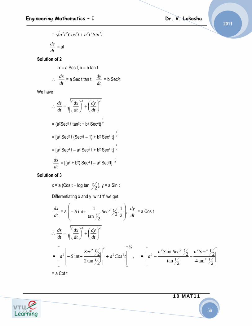
1. x = a (Cos t + t Sin t), y = a (Sin t = t Cos t) 2. x = a Sec t , y = b tan t 3. x = a , y = a Sin t Solution of 1 Given x = a (Cos t + t Sin t), y = a (Sin t – t Cos t ) Differentiating x & y W.r.t ‘t’, we get
= a (-Sin t + Sin t + t Cos t)
= a t cos t
and = a (Cos t – Cos t + t Sin t)
= at Sin t
dydx
dydx
dxds 2
1 ⎟⎠⎞
⎜⎝⎛+
dxdy
2
1 ⎟⎟⎠
⎞⎜⎜⎝
⎛+=
dydx
dyds
xdxds 2tan1+=∴
dyds xCot 21+
xSec2
dxds 2
12 )1( xCot
dyds
+=
dtds
( )2tanlog tCost +
dtdx
dtdx
dtdy
dtdy
22
⎟⎠⎞
⎜⎝⎛+⎟
⎠⎞
⎜⎝⎛=∴
dtdy
dtdx
dtds
Engineering Mathematics – I Dr. V. Lokesha
10 MAT11
56
2011
=
= at
Solution of 2 x = a Sec t, x = b tan t
∴ = a Sec t tan t, = b Sec2t
We have
= (a2Sec2 t tan2t + b2 Sec4t)
= [a2 Sec2 t (Sec2t – 1) + b2 Sec4 t]
= [a2 Sec4 t – a2 Sec2 t + b2 Sec4 t]
= [(a2 + b2) Sec4 t – a2 Sec2t]
Solution of 3
x = a (Cos t + log tan ), y = a Sin t
Differentiating x and y w.r.t ‘t’ we get
= a , = a Cos t
= , =
= a Cot t
tSintatCosta 222222 +
dtds
dtdx
dtdy
22
⎟⎠⎞
⎜⎝⎛+⎟
⎠⎞
⎜⎝⎛=∴
dtdy
dtdx
dtds
21
21
21
dtds 2
1
2t
dtdx
⎟⎟⎟
⎠
⎞
⎜⎜⎜
⎝
⎛+−
21.2
2tan1int 2 tSec
tS
dtdy
22
⎟⎠⎞
⎜⎝⎛+⎟
⎠⎞
⎜⎝⎛=∴
dtdy
dtdx
dtds
21
22
22
2
2tan22int
⎥⎥⎥
⎦
⎤
⎢⎢⎢
⎣
⎡+
⎥⎥
⎦
⎤
⎢⎢
⎣
⎡+− tCosa
t
tSecSa
⎥⎥
⎦
⎤
⎢⎢
⎣
⎡+−
2tan42
2tan2int
2
42222
t
tSecat
tSecSaa

Engineering Mathematics – I Dr. V. Lokesha
10 MAT11
57
2011
Find and for the following curves
1. r = a (1 – Cos θ)
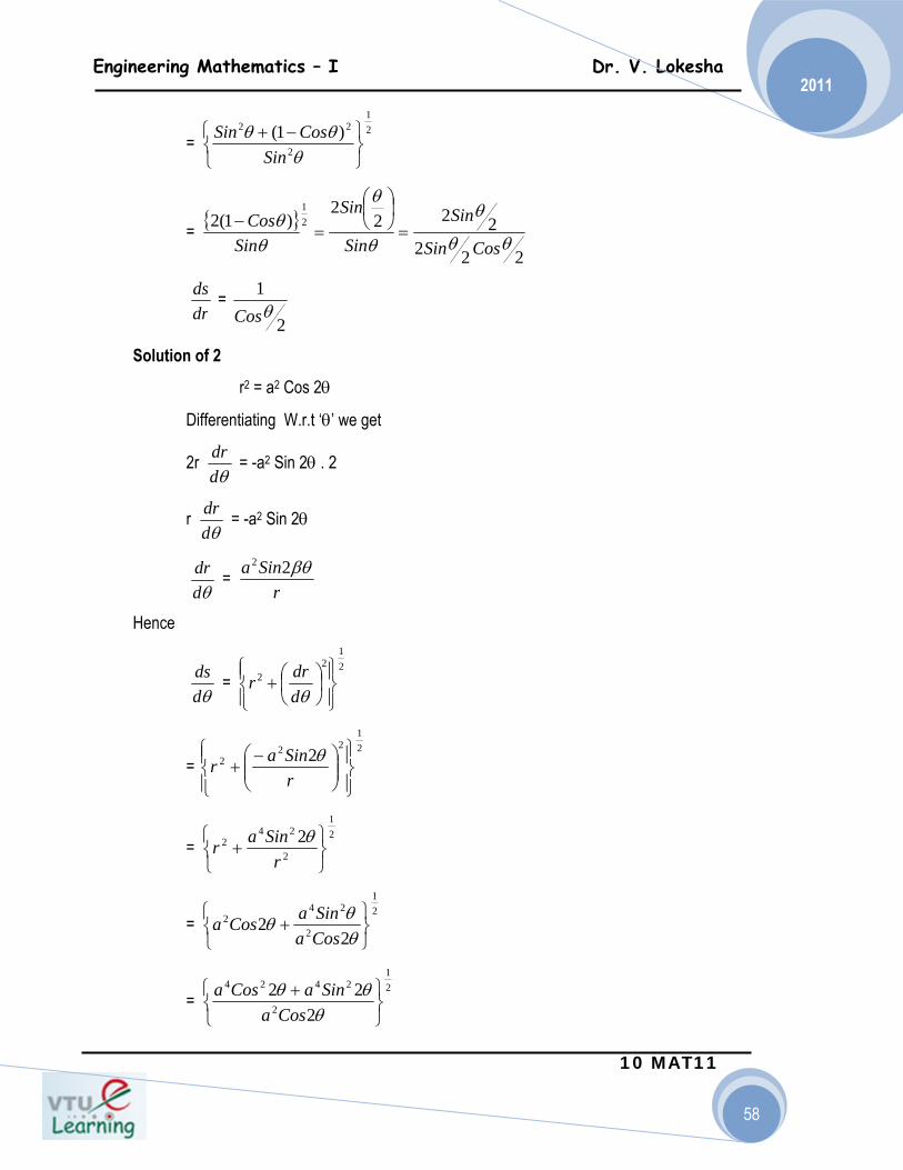
2 .r2 = a2 Cos 2θ
3. r = a eθCot α Solution of 1
r = a (1 – Cos θ)
Differentiating r w.r.t θ we get
= a Sin θ
Hence
=
= {a2 (1 – Cos θ)2 + a2 Sin2 θ}
= {a2 (1 – 2 Cos θ + Cos2θ) + a2 Sin2 θ}
= {a2 – 2a2 Cos θ + a2}
= {2a2 – 2a2 Cos θ}
= a{ 2(1 – Cos θ)}
= a {2 (2 Sin2 )}
= 2 a Sin
And =
=
θdds
θddr
θddr
θdds 2
12
2
⎪⎭
⎪⎬⎫
⎪⎩
⎪⎨⎧
⎟⎠⎞
⎜⎝⎛+
θddrr
21
21
21
21
21
2θ 2
1
θdds
2θ
drds 2
12
21⎪⎭
⎪⎬⎫
⎪⎩
⎪⎨⎧
⎟⎠⎞
⎜⎝⎛+
drdr θ
21
22
22 )1(1⎭⎬⎫
⎩⎨⎧ −
+θθ
SinaCosa
Engineering Mathematics – I Dr. V. Lokesha
10 MAT11
58
2011
=
=
=
Solution of 2
r2 = a2 Cos 2θ
Differentiating W.r.t ‘θ’ we get
2r = -a2 Sin 2θ . 2
r = -a2 Sin 2θ
=
Hence
=
=
=
=
=
21
2
22 )1(
⎭⎬⎫
⎩⎨⎧ −+
θθθ
SinCosSin
{ }
222222
2)1(2 2
1
θθ
θ
θ
θ
θθ
CosSin
Sin
Sin
Sin
SinCos
=⎟⎠⎞
⎜⎝⎛
=−
drds
2
1θCos
θddr
θddr
θddr
rSina βθ22
θdds 2
12
2
⎪⎭
⎪⎬⎫
⎪⎩
⎪⎨⎧
⎟⎠⎞
⎜⎝⎛+
θddrr
21
222 2
⎪⎭
⎪⎬⎫
⎪⎩
⎪⎨⎧
⎟⎟⎠
⎞⎜⎜⎝
⎛ −+
rSinar θ
21
2
242 2
⎭⎬⎫
⎩⎨⎧
+r
Sinar θ
21
2
242
22
⎭⎬⎫
⎩⎨⎧
+θθθ
CosaSinaCosa
21
2
2424
222
⎭⎬⎫
⎩⎨⎧ +
θθθ
CosaSinaCosa
Engineering Mathematics – I Dr. V. Lokesha
10 MAT11
59
2011
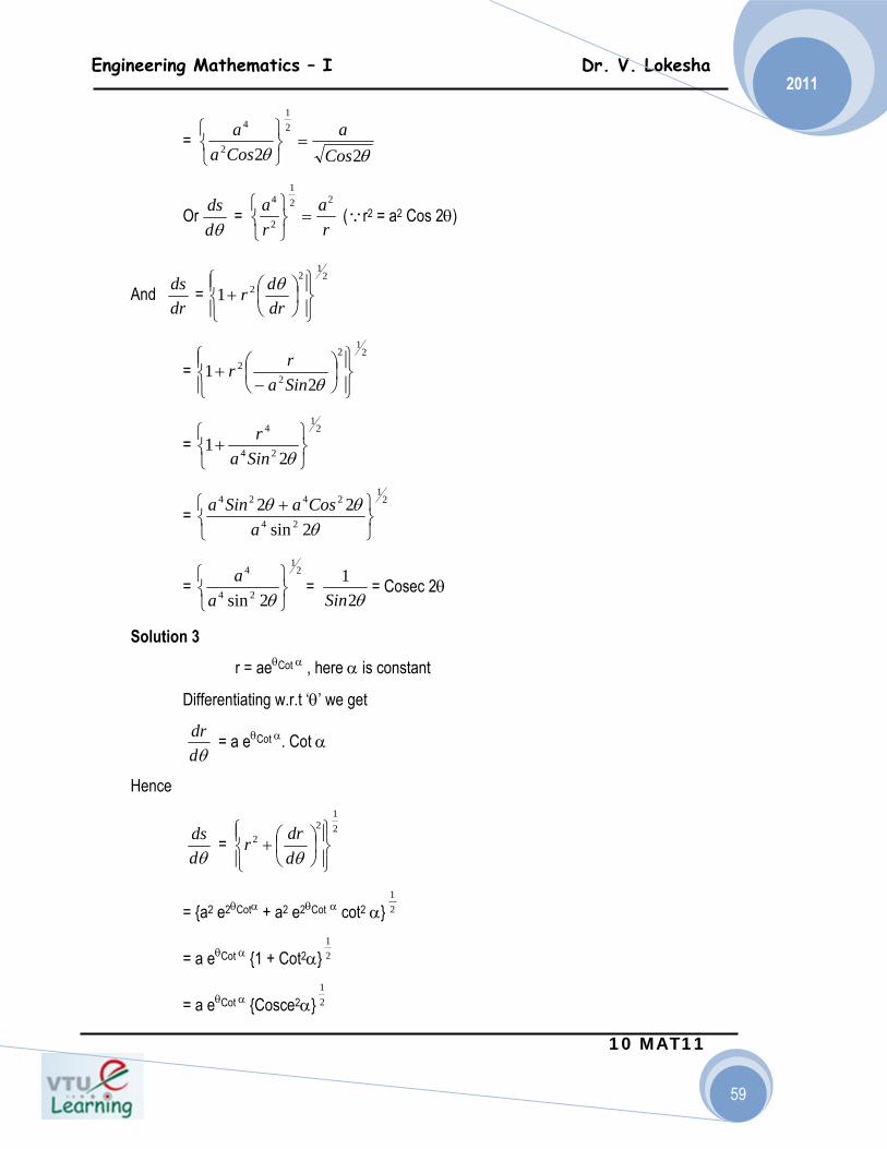
=
Or = (∵r2 = a2 Cos 2θ)
And =
=
=
=
= = = Cosec 2θ
Solution 3
r = aeθCot α , here α is constant
Differentiating w.r.t ‘θ’ we get
= a eθCot α. Cot α
Hence
=
= {a2 e2θCotα + a2 e2θCot α cot2 α}
= a eθCot α {1 + Cot2α}
= a eθCot α {Cosce2α}
θθ 22
21
2
4
Cosa
Cosaa
=⎭⎬⎫
⎩⎨⎧
θdds
ra
ra 22
1
2
4
=⎭⎬⎫
⎩⎨⎧
drds 2
12
21⎪⎭
⎪⎬⎫
⎪⎩
⎪⎨⎧
⎟⎠⎞
⎜⎝⎛+
drdr θ
21
2
22
21
⎪⎭
⎪⎬⎫
⎪⎩
⎪⎨⎧
⎟⎠⎞
⎜⎝⎛
−+
θSinarr
21
24
4
21
⎭⎬⎫
⎩⎨⎧
+θSina
r
21
24
2424
2sin22
⎭⎬⎫
⎩⎨⎧ +
θθθ
aCosaSina
21
24
4
2sin ⎭⎬⎫
⎩⎨⎧
θaa
θ21
Sin
θddr
θdds 2
12
2
⎪⎭
⎪⎬⎫
⎪⎩
⎪⎨⎧
⎟⎠⎞
⎜⎝⎛+
θddrr
21
21
21

Engineering Mathematics – I Dr. V. Lokesha
10 MAT11
60
2011
= a eθCot α Cosce α
and =
=
= {1 + tan2 α}
= {Sec2 α} = Sec α
Exercises:
Find and to the following curves.
1. rn = an Cos nθ
2. r (1 + Cos θ) = a
3. rθ = a
Note:
We have Sin φ = r and
Cos φ =
∴ = Cosφ = (1 – Sin2φ)
= Since P = r Sin φ.
=
θdds
drds 2
12
21⎪⎭
⎪⎬⎫
⎪⎩
⎪⎨⎧
⎟⎠⎞
⎜⎝⎛+
drdr θ
21
2222
2
11⎭⎬⎫
⎩⎨⎧ +
ααθαθ
CotCotCot
eaea
21
21
drds
θdds
dsdθ
dsdr
dsdr 2
1
21
2
2
1 ⎥⎦
⎤⎢⎣
⎡−
rp
dsdr
rpr 22 −

Engineering Mathematics – I Dr. V. Lokesha
10 MAT11
61
2011
=
Q
r+δr P(x,y) φ OR = P r
O X P
R Sin φ =
∴ P = r Sin φ
Prove that with usual notations ⎟⎠⎞
⎜⎝⎛=
drdr θφtan
Let P (r, θ) be any point on the curve r = f (θ)
r OP and POX =θ=∴∧
Let PL be the tangent to the curve at P subtending an angle ψ with the positive direction of
the initial line (x – axis) and φ be the angle between the radius vector OP and the tangent PL.
That is φ=∧
L P O
From the figure we have
drds
∴22 pr
r−
rp
OPOR
=
Engineering Mathematics – I Dr. V. Lokesha
10 MAT11
62
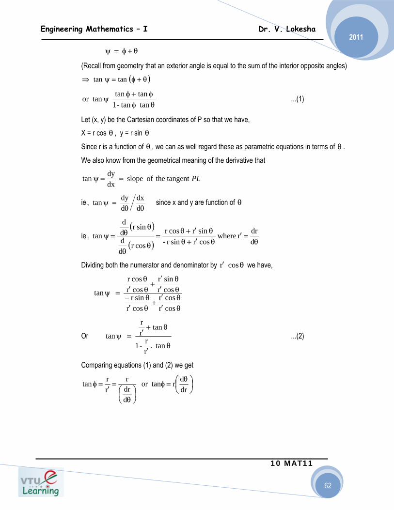
2011 θ+φ=ψ
(Recall from geometry that an exterior angle is equal to the sum of the interior opposite angles) ( )θ+φ=ψ⇒ tan tan
θφφ+φ
ψ tan tan - 1 tan tan tan or …(1)
Let (x, y) be the Cartesian coordinates of P so that we have, X = r cos θ , y = r sin θ
Since r is a function of θ , we can as well regard these as parametric equations in terms of θ .
We also know from the geometrical meaning of the derivative that
PL tangent theof slope dxdy tan ==ψ
ie., ddx
ddy tan
θθ=ψ since x and y are function of θ
ie., ( )
( ) θ=′
θ′+θθ′+θ
=θ
θ
θθ=ψ
ddr r where
cos r sin r -sin r cosr
cosr dd
sin r dd
tan
Dividing both the numerator and denominator by θ′ cos r we have,
θ′θ′
+θ′θ−
θ′θ′
+θ′θ
=ψ
cos r cos r
cos rsin r
cos rsin r
cos r cosr
tan
Or θ
′
θ+′=ψ
tan . rr - 1
an t rr
tan …(2)
Comparing equations (1) and (2) we get
⎟⎠⎞
⎜⎝⎛ θ
=φ⎟⎠⎞
⎜⎝⎛
θ
=′
=φdrdr or tan
ddrr
rr tan

Engineering Mathematics – I Dr. V. Lokesha
10 MAT11
63
2011
Prove with usual notations 2
422 ddr
r1
r1
p1
⎟⎠⎞
⎜⎝⎛
θ+= or
r1 u where
ddu u 1 2
22 =⎟
⎠⎞
⎜⎝⎛+=
θp
Proof : Let O be the pole and OL be the initial line. Let P (r, θ ) be any point on the curve and hence
we have OP = r and θ=∧
POL
Draw ON = p (say) perpendicular from the pole on the tangent at P and let φ be the angle
made by the radius vector with the tangent.
From the figure θ==∧∧
POL 90 PNO
Now from the right angled triangle ONP
OPON sin =φ
ie., φ==φ sin r por rP sin
we have p = r sin φ …(1)
and θ
=φddr
r1 cot …(2)
Squaring equation (1) and taking the reciprocal we get,
Engineering Mathematics – I Dr. V. Lokesha
10 MAT11
64
2011
φ=φ
= cosec r1
p1 ie.,
sin1 .
r1
p 1 2
22222
Or ( )φ+= cot 1 r1
p 1 2
22
Now using (2) we get,
⎥⎥⎦
⎤
⎢⎢⎣
⎡⎟⎠⎞
⎜⎝⎛
θ+=
2
222 ddr
r11
r1
p 1
Or 2
422 ddr
r1
r1
p 1
⎟⎠⎞
⎜⎝⎛
θ+= …(3)
Further, let u r1
=
Differentiating w.r.t. θ we get, 22
42 ddu
ddr
r1
ddu
ddr
r 1
⎟⎠⎞
⎜⎝⎛
θ=⎟
⎠⎞
⎜⎝⎛
θ⇒
θ=⎟
⎠⎞
⎜⎝⎛
θ− , by squaring
Thus (3) now becomes 2
22 d
du u p 1
⎟⎠⎞
⎜⎝⎛
θ+= …(4)
1. Find the angle of intersection of the curves:
( ) ( )θ=θ+= cos-1b r & cos 1 a r
Solution : r = a (1 + cos θ) : r = b(1 – cos θ)
) cos (1 log a log r log θ++=⇒ : log r = log b + log (1 – cos θ)
Differentiating these w.r.t. θ we get
cos1
sin - 0 ddr
r1
θ+θ
+=θ
: cos1
sin 0 ddr
r1
θ−θ
+=θ
( ) ( )( )/2 cos 2
/2 cos /2sin 2 cot 21 θθθ−
=φ : ( ) ( )( )/2 sin 2
/2 cos /2sin 2 cot 22 θθθ
=φ
ie., ( ) ( )/2 /2cot /2 tan - cot 1 θ+π=θ=φ : ( )/2cot cot 2 θ=φ
/2 /2 1 θ+π=φ⇒ : /2 2 θ=φ
Engineering Mathematics – I Dr. V. Lokesha
10 MAT11
65
2011
∴ angle of intersection = /2 /2 - /2 /2 - 21 πθθπφφ =+=
Hence the curves intersect orthogonally. 2. S.T. the curves ( ) ( )θ=θ+= sin-1a r & sin 1 a r cut each other orthogonally
Solution : log r = log a + log (1 + sin θ) : log r = log a + log (1 – sin θ)
Differentiating these w.r.t θ we get
θ+
θ=
θ sin 1 cos
ddr
r1 :
θ−θ
=θ sin 1
cos- ddr
r1
ie., sin 1
cos cot 1 θ+θ
=φ : sin 1
cos- cot 2 θ−θ
=φ
We have θθ
=φθ
θ+=φ
cos -sin - 1 tan and
cossin 1 tan 21
1- cos-
cos cossin-1 tan . tan 2
2
2
2
21 =θθ
=θ−θ
=φφ∴
Hence the curves intersect orthogonally.
3. Find the angle of intersection of the curves:
r = sin θ + cos θ, r = 2 sin θ
Solution : log r = log (sin θ + cos θ) : r = 2 sin θ
( )θ+θ=⇒ cos sin log r log : log r = log 2 + log (sin θ)
Differentiating these w.r.t θ we get
θ+θθθ
=θ cos sin
sin - cos ddr
r1 :
sin cos
ddr
r1
θθ
=θ
ie., ( )( )θ+θ
θθ=φ
tan 1 cos tan -1 cos cot 1 : θ=φ⇒θ=φ cot cot 22
ie., ( ) θ+π=φ⇒θ+π=φ /4 /4cot cot 11
/4 - /4 - 21 π=θθ+π=φφ∴
The angle of intersection is 4/π
Engineering Mathematics – I Dr. V. Lokesha
10 MAT11
66
2011
4. Find the angle of the curves: r = a log θ and r = a/ log θ
Solution : r = a log θ : r = a/ log θ
( )θ+=⇒ log log a log r log : ( )θ= log log - a log r log
Differentiating these w.r.t q, we get,
θθ=
θ . log1
ddr
r1 :
θθ−=
θ . log1
ddr
r1
ie., log
1 cot 1 θθ=φ :
log 1 - cot 2 θθ
=φ
Note : We can not find 21 and φφ explicitly.
θθ=φ∴ log tan 1 : θθ=φ log tan 2
Now consider, θθ=φ log tan 1 : θθ=φ log - tan 2
Now consider, ( )21
21 tan tan 1 log 2 - tan
φφθθ
φφ+
=( )2log1
log2θθ−
θθ= ......…(1)
We have to find θ by solving the given pair of equations :
θ=θ= a/log r and log a r
Equating the R.H.S we have a θ
=θ log
a log
ie., ( ) e logor 1 1 log 2 =θ⇒θ==θ
Substituting ( ) get we1in e =θ
( ) 221 e - 12e tan =φ−φ ( )1 e log =∵
∴ angle of intersection e tan2 e - 1
2e tan - 1-2
1-21 =⎟
⎠⎞
⎜⎝⎛=φφ
5. Find the angle of intersection of the curves:
r = a (1 – cos θ ) and r = 2a cos θ
Solution : r = a (1 – cos θ) : r = 2a cos θ
Taking logarithms we have,
Log r = log a + log (1 – cos θ) : log r = log 2a + log (cos θ)
Differentiating these w.r.t θ, we get,
Engineering Mathematics – I Dr. V. Lokesha
10 MAT11
67
2011
cos - 1
sin ddr
r1
θθ
=θ
: cos
sin - ddr
r1
θθ
=θ
ie., ( ) ( )( ) θ=φθ
θθ=φ tan - cot :
/2 sin 2/2 cos /2sin 2 cot 221
ie., ( )/2cot cot 1 θ=φ : ( )θ+π=φ /2cot cot 2
/2 1 θ=φ⇒ : θ+π=φ /2 2
2 2 / -/2 - /2 21 θπθπθφφ +==−∴ …(1)
Now consider ( ) θ=θ= cos 2a cos - 1 a r
Or ( )1/3 cos or 1 cos 3 -1=θ=θ
Substituting this value in (1) we get,
The angle of intersection ( )1/3 cos . 1/2 2/ -1+π
6. Find the angle of intersection of the curves : θ= ar and θ= / ar
Solution : θ= ar : θ= / ar
θ+=⇒ log a log r log : θ= log - a log r log
Differentiating these w.r.t θ, we get,
θ
=θ
1 ddr
r1 :
θ=
θ1 -
ddr
r1
ie., θ
=φ1 cot 1 :
θ=φ
1 - cot 2
or θ=φ tan 1 : θ=φ - tan 2
Also by equating the R.H.S of the given equations we have
1 1 or a/ a 2 ±=θ⇒=θθ=θ
When and 1- tan 1, tan 1, 21 =φ=φ=θ
When 1 tan 1,- tan 1,- 21 =φ=φ=θ .
/2 - 1 - tan . tan 2121 π=φφ⇒=φφ∴
The curves intersect at right angles.
Engineering Mathematics – I Dr. V. Lokesha
10 MAT11
68
2011
7. Find the pedal equation of the curve: ( ) 2a cos - 1 r =θ
Solution : ( ) 2a cos - 1 r =θ
( ) 2a log cos - 1 log r log =θ+⇒
Differentiating w.r.t θ, we get
θθ
=θ
=θ
θ+
θ cos - 1sin -
ddr
r1or 0
cos - 1sin
ddr
r1
( ) ( )( )
( )/2cot - /2 sin 2
/2 cos /2sin 2- cot 2 θ=θ
θθ=φ∴
ie., ( ) ( )/2 - /2-cot cot θ=φ⇒θ=φ∴
Consider φ= sin r p
( ) ( )/2sin r - por /2-sin r p θ=θ=∴
Now we have, ( ) 2a cos - 1 r =θ …(1)
( )/2sin r - p θ= …(2)
We have to eliminate θ from (1) and (2)
(1) can be put in form ( ) 2a 2/sin 2 . 2 =θr
ie., ( ) a /2 sin r 2 =θ
But p/-r = sin (θ/2), from (2)
ar por a rpr 2
2
2
==⎟⎟⎠
⎞⎜⎜⎝
⎛∴
Thus p2 = ar is the required pedal equation.
8. Find the pedal equation of the curve: r2 = a2 sec 2θ
Solution : r2 = a2 sec 2θ
)2 (sec log a log 2 r log 2 θ+=⇒
Differentiating w.r.t θ , we get,
θ=θθ
θθ=
θ2tan
ddr
r1 ie.,
2 sec2 tan 2 sec 2
ddr
r2
ie., ( ) θπ=φ⇒θπ=φ 2 - /2 2-/2cot cot
Engineering Mathematics – I Dr. V. Lokesha
10 MAT11
69
2011
Consider ( ) θ=θπ=∴φ= 2 cosr p ie., 2-/2sin r p sin r p
Now we have, θ= 2 sec a r 22 …(1)
θ= 2 cosr p …(2)
From (2) p/r = cos 2θ or r/p = sec 2 θ
Substituting in (1) we get, ( )r/p a r 22 = or pr = a2
Thus pr = a2 is the required pedal equation.
9. Find the pedal equation of the curve: rn = an cos nθ
Solution : rn = an cos nθ
( )θ+=⇒ n cos log a logn r logn
Differentiating w.r.t q we get
θ=θθ
θ=
θn tan -
ddr
r1 ie.,
n cosnsin n -
ddr
rn
( ) θ+π=φ⇒θ+π=φ∴ n /2 n /2cot cot
Consider φ= sin r p
( ) θ=θ=π=∴ n cosr p ie., n /2sin r p
Now we have, θ= n cos a r nn …(1)
θ= n cosr p …(2)
( )p/r a r is (2) of econsequenc a as (1) nn =∴
Thus rn + 1 = pan is the required pedal equation.
10. Find the pedal equation of the curve: rm = am (cos mθ + sin mθ)
Solution : rm = am (cos mθ + sin mθ)
Differentiating w.r.t θ, we get,
θ+θθ+θ
=θ msin m cos
m cos m msin m- ddr
rm
ie., ( )( )θ+θ
θθ=
θ+θθθ
=θ mtan 1 m cos
m tan -1 m cos msin m cosmsin -m cos
ddr
r1
( ) θ+π=φ⇒θ+π=φ∴ m /4 m /4cot cot
Engineering Mathematics – I Dr. V. Lokesha
10 MAT11
70
2011
Consider φ= sin r p
( )θ+π=∴ m /4sin r p
ie., ( ) ( )[ ]θπ+θπ= msin /4 cos m cos /4sin r p
ie., ( )θ+θ= msin m cos 2r p
(we have used the formula of sin (A + B) and also the values ( ) ( ) )21/ /4 cos /4 sin =π=π
Now we have, ( )θ+θ= msin m cos a r mm …(1)
( )θ+θ= msin m cos 2r p …(2)
Using (2) in (1) we get,
pa 2 ror r
2p . a r m1mmm == +
Thus pa 2 r m1 m =+ is the required pedal equation.
11. Establish the pedal equation of the curve:
θ+θ= n cos bnsin a r nnn in the form ( ) 2 n 2n22n 2 r ba p +=+
Solution : We have θ+θ= n cos bnsin a r nnn
( )θ+θ=⇒ n cos b nsin a log r logn nn
Differentiating w.r.t θ we get
θ+θθθ
=θ ncosb nsin a
nsin nb - n cos na ddr
rn
nn
nn
Dividing by n, θ+θθθ
=φncosbnsin ansin b - n cosa cot nn
nn
Consider φ= sin r p
Since φ cannot be found, squaring and taking the reciprocal we get,
( )φ+=φ= cot 1 r1
p1or cosec
r1
p1 2
222
22
( )( ) ⎪⎭
⎪⎬⎫
⎪⎩
⎪⎨⎧
θ+θ
θθ+=∴ 2nn
2nn
22n cos bnsin a
nsin b -n cos a1 r1
p1

Engineering Mathematics – I Dr. V. Lokesha
10 MAT11
71
2011
( ) ( )( ) ⎪⎭
⎪⎬⎫
⎪⎩
⎪⎨⎧
θ+θ
θθ+θ+θ= 2nn
2nn2nn
22n cos bnsin a
nsin b - n cos a n cos b nsin a r1
p1 e.,i
( ) ( )( ) ⎪⎭
⎪⎬⎫
⎪⎩
⎪⎨⎧
θ+θ
θ+θ+θ+θ= 2nn
22n222n2
22n cos bnsin a
n sin n cos b n cos n sina r1
p1 e.,i
(product terms cancels out in the numerator)
( )2nn
n 2n 2
22n cos b nsin a
b a . r1
p1 .,ie
θ+θ
+=
( ) ,r
ba . r1
p1 or 2n
n2n 2
22+
= by using the given equation.
( ) 2n 2n 2n 22 r b ap +=+∴ is the required pedal equation.
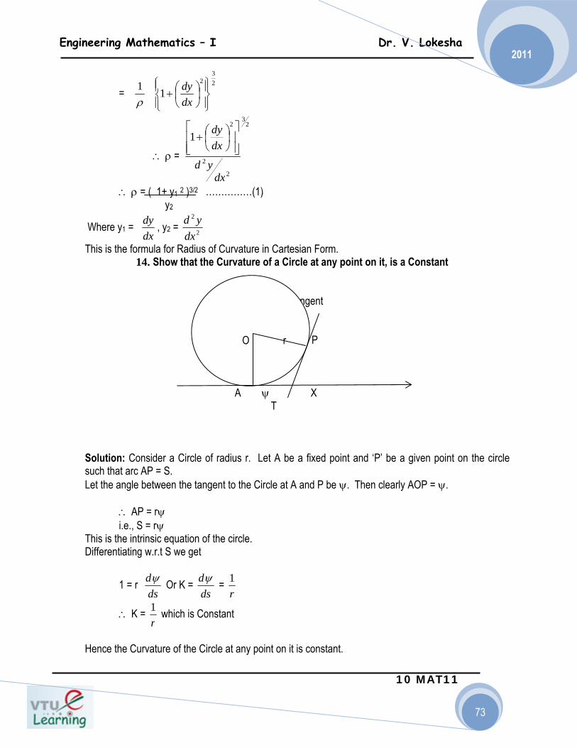
12. Define Curvature and Radius of curvature Solution: A Curve Cuts at every point on it. Which is determined by the tangent drawn. Y y = f (x) Tangent s P (x,y) A O ψ X Let P be a point on the curve y= f (x) at the length ‘s’ from a fixed point A on it. Let the tangent at ‘P’ makes are angle ψ with positive direction of x – axis. As the point ‘P’ moves along curve, both s and ψ vary.
The rate of change ψ w.r.t s, i.e., as called the Curvature of the curve at ‘P’.
The reciprocal of the Curvature at P is called the radius of curvature at P and is denoted by ρ.
dsdψ
ψψρdds
dsd ==∴1
Engineering Mathematics – I Dr. V. Lokesha
10 MAT11
72
2011
(or)
Also denoted ∴K =
K is read it as Kappa.
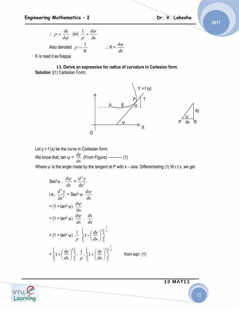
13. Derive an expression for radius of curvature in Cartesian form. Solution :(1) Cartesian Form: Y = f (x) P T A S ψ dy ψ ψ P dx R X O Let y = f (x) be the curve in Cartesian form.
We know that, tan ψ = (From Figure) ----------- (1)
Where ψ is the angle made by the tangent at P with x – axis. Differentiating (1) W.r.t x, we get
Sec2ψ . =
i.e., = Sec2 ψ
= (1 + tan2 ψ)
= (1 + tan2 ψ) .
= (1 + tan2 ψ)
= . . from eqn (1)
ψρ
dds
=∴dsdψ
ρ=
1
K1
=ρdsdψ
dxdy
dxdψ
2
2
dxyd
2
2
dxyd
dxdψ
dxdψ
dxdψ
dxds
ρ1 2
12
1⎪⎭
⎪⎬⎫
⎪⎩
⎪⎨⎧
⎟⎠⎞
⎜⎝⎛+
dxdy
⎪⎭
⎪⎬⎫
⎪⎩
⎪⎨⎧
⎟⎠⎞
⎜⎝⎛+
2
1dxdy
ρ1 2
12
1⎪⎭
⎪⎬⎫
⎪⎩
⎪⎨⎧
⎟⎠⎞
⎜⎝⎛+
dxdy
Engineering Mathematics – I Dr. V. Lokesha
10 MAT11
73
2011
=
∴ ρ =
∴ ρ = ( 1+ y1 2 )3/2 ……………(1) y2
Where y1 = , y2 =
This is the formula for Radius of Curvature in Cartesian Form. 14. Show that the Curvature of a Circle at any point on it, is a Constant
Tangent
PP P
A ψ X T Solution: Consider a Circle of radius r. Let A be a fixed point and ‘P’ be a given point on the circle such that arc AP = S. Let the angle between the tangent to the Circle at A and P be ψ. Then clearly AOP = ψ. ∴ AP = rψ i.e., S = rψ This is the intrinsic equation of the circle. Differentiating w.r.t S we get
1 = r Or K = =
∴ K = which is Constant
Hence the Curvature of the Circle at any point on it is constant.
ρ1 2
32
1⎪⎭
⎪⎬⎫
⎪⎩
⎪⎨⎧
⎟⎠⎞
⎜⎝⎛+
dxdy
23
2
2
2
1
dxyd
dxdy
⎥⎥⎦
⎤
⎢⎢⎣
⎡⎟⎠⎞
⎜⎝⎛+
dxdy
2
2
dxyd
dsdψ
dsdψ
r1
r1
O r

Engineering Mathematics – I Dr. V. Lokesha
10 MAT11
74
2011
15. Derive an expression for radius of curvature in parametric form.
Solution: We have ρ = (1 + y 12 )3/2
y2 Let x =f (t), y = g (t) be the curve in Parametric Form.
Then y1 =
Y2 = = =
= . .
=
∴ Y2 =
Substituting Y1 and Y2 in equation 1.
ρ = , we get
ρ =
-------------------- (2)
Equation (2) is called the Radius of Curvature in Parametric Form.
•
•
==X
Y
dtdx
dtdy
dxdy
2
2
dxyd
dxd
⎟⎠⎞
⎜⎝⎛
dxdy
dxd
⎟⎟⎟
⎠
⎞
⎜⎜⎜
⎝
⎛•
•
X
Ydtd
⎟⎟⎟
⎠
⎞
⎜⎜⎜
⎝
⎛•
•
X
Ydxdt
dtd
⎟⎟⎟
⎠
⎞
⎜⎜⎜
⎝
⎛•
•
X
Y
⎟⎟⎟⎟
⎠
⎞
⎜⎜⎜⎜
⎝
⎛
dtdx1
dtd
⎟⎟⎟
⎠
⎞
⎜⎜⎜
⎝
⎛•
•
X
Y•
X
1
( )2xxyyx −
•
)(
1
X
3
⎟⎠⎞
⎜⎝⎛
−•
•
x
xyyX
( )2
232
11yY+
( )( )
( )3
23
21
xxyyx
xY
−⎥⎦⎤
⎢⎣⎡ +
( ) ( )[ ]xyyx
yx−
+=
2322
ρ
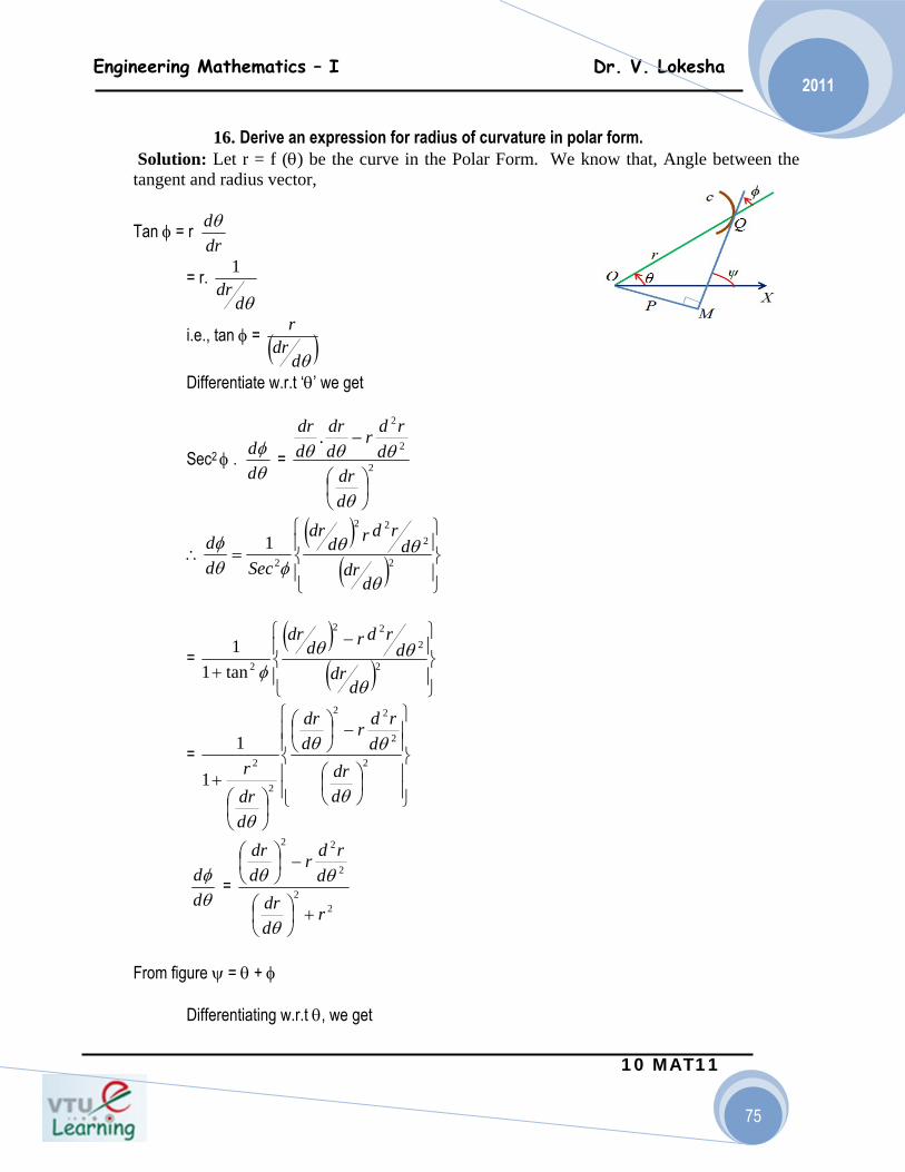
Engineering Mathematics – I Dr. V. Lokesha
10 MAT11
75
2011
16. Derive an expression for radius of curvature in polar form.
Solution: Let r = f (θ) be the curve in the Polar Form. We know that, Angle between the tangent and radius vector,
Tan φ = r
= r.
i.e., tan φ =
Differentiate w.r.t ‘θ’ we get
Sec2 φ . =
=
=
=
From figure ψ = θ + φ Differentiating w.r.t θ, we get
drdθ
θddr
1
( )θddr
r
θφ
dd
2
2
2
.
⎟⎠⎞
⎜⎝⎛
−
θ
θθθ
ddr
drdr
ddr
ddr
( )( ) ⎪
⎭
⎪⎬
⎫
⎪⎩
⎪⎨
⎧=∴ 2
222
2
1
θ
θθφθ
φ
ddr
drdrd
dr
Secdd
( )( ) ⎪
⎭
⎪⎬
⎫
⎪⎩
⎪⎨
⎧ −
+ 2
222
2tan11
θ
θθφ
ddr
drdrd
dr
⎪⎪⎭
⎪⎪⎬
⎫
⎪⎪⎩
⎪⎪⎨
⎧
⎟⎠⎞
⎜⎝⎛
−⎟⎠⎞
⎜⎝⎛
⎟⎠⎞
⎜⎝⎛
+2
2
22
2
2
1
1
θ
θθ
θddr
drdr
ddr
ddrr
θφ
dd
22
2
22
rddr
drdr
ddr
+⎟⎠⎞
⎜⎝⎛
−⎟⎠⎞
⎜⎝⎛
θ
θθ

Engineering Mathematics – I Dr. V. Lokesha
10 MAT11
76
2011
= 1 +
∴ = 1 +
=
Also we know that =
Now, ρ= = .
= .
ρ ----------- (3)
Where r1 = , r2 =
Equation (3) as called the radius of curvature in Polar form.
17. Derive an expression for radius of curvature in pedal form.
Solution: Let p = r Sin φ be the curve in Polar Form. We have p = r Sin φ Differentiating p W.r.t r, we get
= Sin φ + r Cos φ
θψ
dd
θφ
dd
θψ
dd
22
2
22
rddr
drdr
ddr
+⎟⎠⎞
⎜⎝⎛
−⎟⎠⎞
⎜⎝⎛
θ
θθ
θψ
dd
22
2
222 2
rddr
drdr
ddrr
+⎟⎠⎞
⎜⎝⎛
−⎟⎠⎞
⎜⎝⎛+
θ
θθ
θdds 2
12
2
⎪⎭
⎪⎬⎫
⎪⎩
⎪⎨⎧
⎟⎠⎞
⎜⎝⎛+
θddrr
ψdds
θdds
ψθ
dd
21
22
⎪⎭
⎪⎬⎫
⎪⎩
⎪⎨⎧
⎟⎠⎞
⎜⎝⎛+
θddrr
2
222
22
2θθ
θ
drdr
ddrr
rddr
−⎟⎠⎞
⎜⎝⎛+
+⎟⎠⎞
⎜⎝⎛
( )2
21
2
232
12
2 rrrrrr
−++
=
θddr
2
2
θdrd
drdp
drdφ
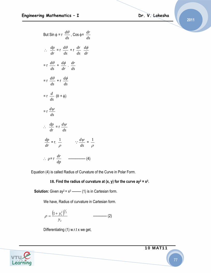
Engineering Mathematics – I Dr. V. Lokesha
10 MAT11
77
2011
But Sin φ = r , Cos φ=
∴ = r + r
= r + .
= r + r
= r (θ + φ)
= r
∴ = r
= r. ∵ =
∴ ρ= r --------------- (4)
Equation (4) is called Radius of Curvature of the Curve in Polar Form.
18. Find the radius of curvature at (x, y) for the curve ay2 = x3.
Solution: Given ay2 = x3 -------- (1) is in Cartesian form. We have, Radius of curvature in Cartesian form.
------------ (2)
Differentiating (1) w.r.t x we get,
dsdθ
dsdr
drdp
dsdθ
dsdr
drdφ
dsdθ
drdφ
dsdr
dsdθ
dsdφ
dsd
dsdψ
drdp
dsdψ
drdp
ρ1
dsdψ
ρ1
dpdr
( )2
232
11yy+
=ρ

Engineering Mathematics – I Dr. V. Lokesha
10 MAT11
78
2011
a 2y
Differentiating y1 w.r.t ‘x’ we get
Substitute Y1 and Y2 in (2), we get.
19. Find the radius of curvature at (x,y) for the curve y = c log Sec
Solution: Given y = c log Sec -------- (1)
Differentiating (1) w.r.t x, we get
= c tan . = tan
Differentiating y1 W.r.t x we get
=
Substitute y1 and y2 in
∴
ρ =
ax
axa
xayxy
dxdyx
dxdy
23
2
3233
21
3
22
12 =
⎟⎟⎠
⎞⎜⎜⎝
⎛===⇒=
axy
23
1 =∴
xaxadxydy
43
21
23
2
2
2 ===
( )a
xax6
94 23
+=ρ
⎟⎠⎞
⎜⎝⎛
cx
⎟⎠⎞
⎜⎝⎛
cx
⎟⎠⎞
⎜⎝⎛
⎟⎠⎞
⎜⎝⎛
⎟⎠⎞
⎜⎝⎛
=cx
cxSec
cxSec
cy tan.1.1 ⎟⎠⎞
⎜⎝⎛
cx
c1
⎟⎠⎞
⎜⎝⎛
cx
⎟⎠⎞
⎜⎝⎛=
cxSecy 2
2 c1
c1
⎟⎠⎞
⎜⎝⎛
cxSec 2
( )2
232
11yy+
=δ
( )[ ]( )
( )[ ]( )cxSec
c
cxSec
cxSec
c
cx
2
23
2
2
23
2
11tan1
=+
=δ
( )cxcSec
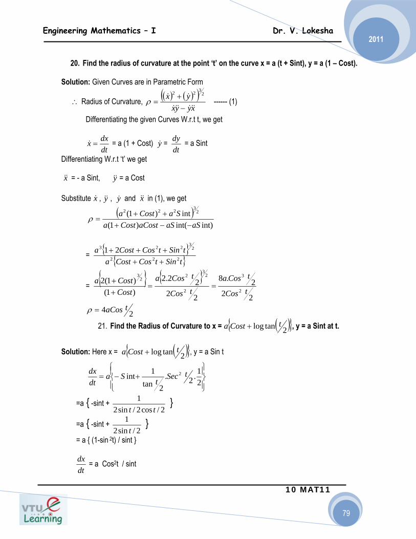
Engineering Mathematics – I Dr. V. Lokesha
10 MAT11
79
2011
20. Find the radius of curvature at the point ‘t’ on the curve x = a (t + Sint), y = a (1 – Cost).
Solution: Given Curves are in Parametric Form
∴ Radius of Curvature, ------ (1)
Differentiating the given Curves W.r.t t, we get
= a (1 + Cost) = = a Sint
Differentiating W.r.t ‘t’ we get
= - a Sint, = a Cost Substitute , , and in (1), we get
=
=
21. Find the Radius of Curvature to x = , y = a Sint at t. Solution: Here x = , y = a Sin t
=a { -sint + }
=a { -sint + } = a { (1-sin 2t) / sint } = a Cos2t / sint
( ) ( )( )xyyx
yx−
+=
2322
ρ
dtdxx = y
dtdy
x y
x y y x
( )int)int()1(
int)1( 23222
aSaSaCostCostaSaCosta
−−+++
=ρ
{ }{ }tSintCosCosta
tSintCosCosta222
23223 21
+++++
{ } { }222.8
2222.2
)1()1(2
2
3
2
23
22
3
tCos
tCosatCos
tCosa
CostCosta
==++
24 taCos=ρ
( ){ }2tanlog tCosta +
( ){ }2tanlog tCosta +
⎪⎭
⎪⎬⎫
⎪⎩
⎪⎨⎧
+−=21.2.
2tan1int 2 tSec
tSa
dtdx
2/cos2/sin21
tt
2/sin21
t
dtdx
Engineering Mathematics – I Dr. V. Lokesha
10 MAT11
80
2011
= = tant
Differentiating W.r.t ‘x’ we get
Substitute & in , we get
i.e.,
∴ρ = a Cot t.
22. Find the Radius of Curvature to at
Solution: Given -------------- (1) Differentiating (1) w.r.t to ‘x’ we get
i.e., (From (1))
----------- (2)
aCostdxdyand =
dtdxdtdy
dxdy
//
=∴ttta
aCostsin/coscos
tdxdy tan=∴
int
1.12
2222
2
StaCos
tSec
dtdx
tSecdxdttSec
dxyd
===
int1 42
2
tSSecadx
yd==
dxdy
2
2
dxyd ( )
2
232
11yy+
=ρ
( ) aCottSCosta
tSSectaSec
tSSeca
t===
+=
intintint1tan1
4
3
4
232
ρ
ayx =+ ⎟⎠⎞
⎜⎝⎛
4,
4aa
ayx =+
02
12
1=+
dxdy
yx
( )x
xaxy
dxdyy −
−=−==1
xay −= 11
Engineering Mathematics – I Dr. V. Lokesha
10 MAT11
81
2011
Also -------------- (3)
At the given point
Then = - 1 &
∴ Substitute y1 and y2 in
ρ =
ρ
23. Show that for the Cardioids r = a (1 + Cosθ), ρ2 / r 2 is a constant Solution: r = a (1 + Cosθ)
= - a Sinθ
We have,
, is Pedal Equation.
= a2Sin2θ
=
=
23
23
2
2
222
1
x
axadx
ydy =⎟⎠⎞
⎜⎝⎛−−== −
⎟⎠⎞
⎜⎝⎛
4,
4aa
2
11 aay −=
( ) aa
ay 4
421
232 =−=
( )2
232
11yy+
=ρ
( )24
224
24
)1(1 23
232 aaa
a===
−+
2a
=
θddr
2
422
111⎟⎠⎞
⎜⎝⎛+=
θddr
rrP
42
11rr
+
4
2222
4
222 )1(r
SinaCosar
Sinar θθθ ++=
+
4
2 )1(2r
Cosa θ+

Engineering Mathematics – I Dr. V. Lokesha
10 MAT11
82
2011
(∵ r = a (1 + Cosθ)
Differentiating w.r.t ‘P’ we get
2P =
Now,
And
24. Find the Radius of Curvature of the Curve
Solution: Given
Differentiating w.r.t to P, we get
⎟⎠⎞
⎜⎝⎛=∴
ar
ra
P 4
2
2
21
θCosar
+=∴ 1
32
21ra
P=
arP2
32 =∴
dpdrr
a23
21
234
rap
dpdr
=
rap
dpdrr
34
==ρ
98
2.
916
9161 3
3
2
2
22
2
2 aa
rra
rpa
rr==⎥
⎦
⎤⎢⎣
⎡=
ρ
22
2
222
111ba
rbaP
−+=
22
2
222
111ba
rbaP
−+=
dpdrr
baP212
223
−=
−
rpba
dpdr
3
22
=∴
3
22
3
22
..pba
rpbar
dpdrr ===∴ ρ
Engineering Mathematics – I Dr. V. Lokesha
10 MAT11
83
2011
25. Find the Radius of Curvature at (r,θ) on r =
Solution: Given r =
Differentiating w.r.t to ‘θ’ we get
We have
Differentiating above result w.r.t to‘P’ we get
θa
θa
θθθθθraa
ddr −
=−
=−
=1.2
θθr
ddr −
=
2
422
111⎟⎠⎞
⎜⎝⎛+=
θddr
rrP
2222
2
42
1111θθ rr
rrr
+=+=
⎟⎟⎠
⎞⎜⎜⎝
⎛ +=⎟
⎠⎞
⎜⎝⎛ += 2
2
2222
111111θ
θθ rrP
12 +=∴
θ
θrP
22
2
22
.
1
.
1 rara
ra
rarrP
+=
+
=+
=θ
θ
( )22
22
22 22
1..1
radpdrr
raar
dpdrara
+
/+/
−+=
dpdr
raararara ⎟⎟
⎠
⎞⎜⎜⎝
⎛
+−+=+
22
22222 .
dpdr
raararara
22
22222 ).(
+
−+=+

Engineering Mathematics – I Dr. V. Lokesha
10 MAT11
84
2011
Thus,
Exercises:
(1) Find the Radius of the Curvature at the point (s, ψ) on S = a log tan
(2) Find the Radius of the Curvature of xy = C2 at (x,y) (3) Find the Radius of the Curvature of xy3 = a4 at (a,a) (4) Find the Radius of Curvature at the point θ on x = C Sin 2θ (1 + Cos 2θ), y = C Cos 2θ (1 – Cos 2θ) (5) If ρ1 and ρ2 are the radii of curvature at the extremities of any chord of the cardiode
r = a (1 + Cosθ) which posses through the Pole prove that
( )dpdrarara 32222 =++
( )dpdr
ara
=+
3
2322
( )3
2322..
arar
dpdrr +
==ρ
( ) 2322
3 raar
+=∴ ρ
⎟⎠⎞
⎜⎝⎛ +
24ψπ
916 2
22
21
a=+ ρρ

Engineering Mathematics – I Dr. V. Lokesha
10 MAT11
85
2011
DIFFERENTIAL CALCULUS – III PARTIAL DIFFERENTIATION Introduction :- Partial differential equations abound in all branches of science and engineering and many areas of business. The number of applications is endless. Partial derivatives have many important uses in math and science. We shall see that a partial derivative is not much more or less than a particular sort of directional derivative. The only trick is to have a reliable way of specifying directions ... so most of this note is concerned with formalizing the idea of direction So far, we had been dealing with functions of a single independent variable. We will now consider functions which depend on more than one independent variable; Such functions are called functions of several variables.
Geometrical Meaning Suppose the graph of z = f (x,y) is the surface shown. Consider the partial derivative of f with respect to x at a point (x0, y0). Holding y constant and varying x, we trace out a curve that is the intersection of the surface with the vertical plane y = y0. The partial derivative fx(x0,y0). measures the change in z per unit increase in x along this curve. That is, fx(x0, y0) is just the slope of the curve at (x0, y0). The geometrical interpretation of fy(x0, y0). is analogous.

Engineering Mathematics – I Dr. V. Lokesha
10 MAT11
86
2011
Real-World Applications: Rates of Change: In the Java applet we saw how the concept of partial derivative could be applied geometrically to find the slope of the surface in the x and y directions. In the following two examples we present partial derivatives as rates of change. Specifically we explore an application to a temperature function ( this example does have a geometric aspect in terms of the physical model itself) and a second application to electrical circuits, where no geometry is involved. I. Temperature on a Metal Plate The screen capture below shows a current website illustrating thermal flow for chemical engineering. Our first application will deal with a similar flat plate where temperature varies with position. * The example following the picture below is taken from the current text in SM221,223: Multivariable Calculus by James Stewart.
Engineering Mathematics – I Dr. V. Lokesha
10 MAT11
87
2011
Suppose we have a flat metal plate where the temperature at a point (x,y) varies according to position. In particular, let the temperature at a point (x,y) be given by, where T is measured in oC and x and y in meters. Question: what is the rate of change of temperature with respect to distance at the point (2,1) in (a) the x-direction? and (b) in the y-direction ? Let's take (a) first. What is the rate of change of temperature with respect to distance at the point (2,1) in (a) the x-direction? What observations and translations can we make here? Rate of change of temperature indicates that we will be computing a type of derivative. Since the temperature function is defined on two variables we will be computing a partial derivative. Since the question asks for the rate of change in the x-direction, we will be holding y constant. Thus, our question now becomes: What is at the point (2,1)? Conclusion : The rate of change of temperature in the x-direction at (2,1) is degrees per meter; note this means that the temperature is decreasing !
2 2( , ) 60 /1T x y x y= + +
dTdx
2 2 2 2 1
2 2 2
2
( , ) 60 /1 60(1 )
60(2 )(1 )
20(2,1) 60(4)(1 4 1) 3
T x y x y x yT x x yxT
x
−
−
−
= + + = + +∂ = − + +∂∂ −= − + + =∂
203
−

Engineering Mathematics – I Dr. V. Lokesha
10 MAT11
88
2011
Part (b): The rate of change of temperature in the y-direction at (2,1) is computed in a similar manner. Conclusion : The rate of change of temperature in the y-direction at (2,1) is degrees per meter; note this means that the temperature is decreasing !
II. Electrical Circuits: Changes in Current The following is adapted from an example in a former text for SM221,223 Multivariable
Calculus by Bradley and Smith. * In an electrical circuit with electromotive force (EMF) of E volts and resistance R ohms, the current, I, is I=E/R amperes. Question: (a) At the instant when E=120 and R=15 , what is the rate of change of current with respect to voltage. (b) What is the rate of change of current with respect to resistance? (a) Even though no geometry is involved in this example, the rate of change questions can be answered with partial derivatives. we first note that I is a function of E and R, namely, I(E,R) = ER-1
2 2 2 2 1
2 2 2
2
( , ) 60 /1 60(1 )
60(2 )(1 )
10(2,1) 60(2)(1 4 1) 3
T x y x y x yT y x yxT
x
−
−
−
= + + = + +∂ = − + +∂∂ −= − + + =∂
103
−
Engineering Mathematics – I Dr. V. Lokesha
10 MAT11
89
2011
The rate of change of current with respect to voltage = the partial derivative of I with respect to voltage, holding resistance constant is when E=120 and R=15 , we have verbal conclusion : If the resistance is fixed at 15 ohms, the current is increasing with respect to voltage at the rate of 0.0667 amperes per volt when the EMF is 120 volts. Part (b): What is the rate of change of current with respect to resistance? Using similar observations to part (a) we conclude: The partial derivative of I with respect to resistance, holding voltage constant = when E=120 and R=15 , we have Conclusion : If the EMF is fixed at 120 volts, the current is decreasing with respect to resistance at the rate of 0.5333 amperes per ohm when the resistance is 15 ohms.
Key Words :- Then the partial derivative of z w.r.t x is given by The partial derivative of z w.r.t y is given by
1I RE−∂ =∂
115 0.0667IE
−∂ = ≈∂
1I ERE−∂ =∂
1(120,15) 120(15) 0.5333IE
−∂ = − ≈ −∂
0
( , ) ( , )limxx
z f x x y f x yzx xδ
δδ→
∂ + −= =
∂
0
( , ) ( , )limyy
z f x y y f x yzy yδ
δδ→
∂ + −= =
∂
Engineering Mathematics – I Dr. V. Lokesha
10 MAT11
90
2011
1. If ( )byaxsin e u by-ax += show that u ab 2a - =∂∂
∂∂
yu
xub
Solution : ( )by ax sin e u by-ax +=
( ) ( )by ax sin a.e a . by ax cos e xu by-axby -ax +++=
∂∂
∴
( ) ua by ax cos e a xu e.,i by -ax ++=
∂∂ …(1)
Also ( ) ( ) ( )by ax sin e b- b . by ax cos e by-axby -ax +++=∂∂
xu
( ) bu by ax cos e b yu .,ie by -ax −+=
∂∂ …(2)
Now yu a
xu b
∂∂
=∂∂ by using (1) and (2) becomes
( ) ( ) abu byax cos abe -abu by ax cos abe by-axbyax ++++= −
= 2 abu
Thus abu 2 yu a -
xu b =
∂∂
∂∂
2. If ( ) that prove ,by-ax f e u byax +=
abu2yu a
xu b =
∂∂
=∂∂
Solution : ( )by -ax f eu byax+= , by data
( ) ( )by -ax fae a by-ax f . e xu byaxby ax ++ +′=
∂∂
Or ( ) u a by-ax f . e a by ax +′=∂∂ +
xu …(1)
Next, ( ) ( ) ( )by -ax f e b b- . by-ax f e yu by ax by ax ++ +′=
∂∂
Or ( ) ba by -ax f e b yu byax +′−=
∂∂ + …(2)
Now consider L.H.S yua
xu b
∂∂
+∂∂
=

Engineering Mathematics – I Dr. V. Lokesha
10 MAT11
91
2011
( ){ } ( ){ }bu by -ax f be- a au by -ax f ae b byaxbyax +′++′= ++
( ) ( ) abu by -ax fe ab-abu by -ax f e ab by ax byax +′+′= ++
= 2abu = R.H.S
Thus u b a 2 yua
xu b =
∂∂
+∂∂
3. If 222 z y x log u ++= , show that ( ) 1 zu
yu
xu z y x 2
2
2
2
2
2222 =⎟⎟
⎠
⎞⎜⎜⎝
⎛∂∂
+∂∂
+∂∂
++
Solution : By data ( )222222 zyx log 21 zy x log u ++=++=
The given u is a symmetric function of x, y, z, (It is enough if we compute only one of the required partial derivative)
222222 y 2 . 1 .
21
zxxx
zyxxu
++=
++=
∂∂
⎟⎟⎠
⎞⎜⎜⎝
⎛
++∂∂
=⎟⎠⎞
⎜⎝⎛
∂∂
∂∂
=∂∂
222
2
zy u u
xx
xxxx2
ie., ( )
( ) ( )2222
222
2222
222
zy
zy zy
2 . - 1 zy
++
−+=
++
++
x
x
x
xxx
( )2222
222
2
2
zy
zy u ++
−+=
∂∂
∴x
xx
…(1)
Similarly ( )2222
222
2
2
zy
xz u ++
−+=
∂∂
∴x
yy
…(2)
( )2222
222
2
2
zy
yx u ++
−+=
∂∂
x
zz
…(3)
Adding (1), (2) and (3) we get,
( ) 2222222
222
2
2
2
2
2
2
zy1
zy
zy uu u ++
=++
++=
∂∂
+∂∂
+∂∂
xx
xzyx
Thus ( ) 1 zu
yu u zy 2
2
2
2
2
2222 =⎟⎟
⎠
⎞⎜⎜⎝
⎛
∂∂
+∂∂
+∂∂
++x
x

Engineering Mathematics – I Dr. V. Lokesha
10 MAT11
92
2011
4. If u = log (tan x + tan y + tan z), show that, sin 2x ux + sin 2y uy + sin 2z uz = 2
Solution : u = log (tan x + tan y + tan z) is a symmetric function.
z tan y tan tan
sec u2
++=
xx
x
( )z tan y tan tan .sec cos sin 2 u 2 sin
2
++=
xxxxx x
Or z tan y tan tan
tan 2 u 2 sin++
=x
xx x …(1)
Similarly z tan y tan tan
tan 2 u 2 sin++
=x
yy y …(2)
z tan y tan tan
tan 2 u 2 sin++
=x
zz y …(3)
Adding (1), (2) and (3) we get,
( )( ) 2
z tan y tan x tanz tan y tan tan x 2 u 2zsin u2y sin u 2 sin zy =
++++
=++xx
Thus 2 u 2zsin u2y sin u2x sin zyx =++
5. If u = log (x3 + y3 + z3 – 3xyz) then prove that zyx
3 zu
yu
xu
++=
∂∂
+∂∂
+∂∂ and hence show
that ( )2
2
zy9- u ++
=⎟⎟⎠
⎞⎜⎜⎝
⎛∂∂
+∂∂
+∂∂
xzyx
Solution : u = log (x3 + y3 + z3 – 3xyz) is a symmetric function
yz3 - zy3yz - 3 u333
2
xxx
x ++=
∂∂ …(1)
yz3 - zy3zx - 3 u333
2
xxy
y ++=
∂∂ …(2)
yz3 - zy3xy - 3 u
333
2
xxz
z ++=
∂∂ …(3)
Adding (1), (2) and (3) we get,
Engineering Mathematics – I Dr. V. Lokesha
10 MAT11
93
2011
( )( )yz3zy
zyzyzy 3 zu u u
333
222
xxxxx
yx −++−−−++
=∂∂
+∂∂
+∂∂
Recalling a standard elementary result,
( ) ( )cabcabcba cba abc3cba 222333 −−−++++=−++
We have,
( )( ) ( )xxxx
xxxx zyzyzy zy
zyzyzy 3 zu
yu u
222
222
−−−++++−−−++
=∂∂
+∂∂
+∂∂
Thus zy
3 zu
yu u
++=
∂∂
+∂∂
+∂∂
xx
Further u z
y
2
⎟⎟⎠
⎞⎜⎜⎝
⎛∂∂
+∂∂
+∂∂x
u z
y
z
y
⎟⎟⎠
⎞⎜⎜⎝
⎛∂∂
+∂∂
+∂∂
⎟⎟⎠
⎞⎜⎜⎝
⎛∂∂
+∂∂
+∂∂
=xx
zu
yu u
z
y ⎟⎟
⎠
⎞⎜⎜⎝
⎛∂∂
+∂∂
+∂∂
⎟⎟⎠
⎞⎜⎜⎝
⎛∂∂
+∂∂
+∂∂
=xx
z y
3 z
y
⎟⎟⎠
⎞⎜⎜⎝
⎛++⎟⎟
⎠
⎞⎜⎜⎝
⎛∂∂
+∂∂
+∂∂
=xx
, by using the earlier result.
⎟⎟⎠
⎞⎜⎜⎝
⎛++∂
∂+⎟⎟
⎠
⎞⎜⎜⎝
⎛++∂
∂+⎟⎟
⎠
⎞⎜⎜⎝
⎛++∂
∂=
z y 3
z
z y 3
y
zyx3
x
xx
( ) ( ) ( ) ( )2222 zy
9 zy
3 zy
3 zy
3 ++
−=
++−
+++
−+
++−
=xxxx
Thus ( )2
2
zy9- u
z
y
x ++=⎟⎟
⎠
⎞⎜⎜⎝
⎛∂∂
+∂∂
+∂∂
x
Engineering Mathematics – I Dr. V. Lokesha
10 MAT11
94
2011
6. If ( ) θ=θ== sin r y , cosr and rf u x ,
prove that ( ) ( )r r1 r 2
2
2
2
ffyu
xu ′+′′=
∂∂
+∂∂
Solution :Observing the required partial derivative we conclude that u must be a function of x, y. But
u = f( r) by data and hence we need to have r as a function of x, y. Since x = r cos θ, y = r
sin θ we have x2 + y2 = r2.
( ) 22 yx r wherer f u have we +==∴
( ) ( ) ( ) and .
rr - r
rr u 2
222
32
2
xfxfx
′′+
′=
∂∂
( ) ( ) ( ) .
rr - r
rr u 2
222
32
2yfyf
y′′
+′
=∂∂
Adding these results we get,
( ) ( ){ } ( ) ( )222
22232
2
2
2y
rrf y - 2
rrf u u
+′′
++′
=∂∂
+∂∂ xxx
yx
( ) ( ) ( ) ( )r r r1 r .
rr r .
rr 2
22
3 ffff ′′+′=′′
+′
=
Thus ( ) ( )r r1 r 2
2
2
2
ffyu
xu ′+′′=
∂∂
+∂∂
7. Prove that nuyuy
xux =
∂∂
+∂∂
Proof : Since u = f (x, y) is a homogeneous function of degree n we have by the definition,
( )y/x g x u n= …(1)
Let us differentiate this w.r.t x and also w.r.t.y
( ) ( )xxx
xx y/ g n y- . y/ g . xu 1 -n
2n +⎟
⎠⎞
⎜⎝⎛′=
∂∂
∴
ie., ( ) ( )xxxxx
y / g n y/ gy u 1 -n 2 -n +′=∂∂ …(2)
Also ( ) ⎟⎠⎞
⎜⎝⎛′=
∂∂
xxx
y1 . y/ g . u n
Engineering Mathematics – I Dr. V. Lokesha
10 MAT11
95
2011
ie., ( ) y/ g . u 1 -n xxy
′=∂∂ …(3)
Now consider yx
x∂∂
+∂∂ uy u as a consequence of (2) and (3)
( ) ( )[ ] ( )[ ]xxxxxxx y / g y y/ g n y/ gy - 1 -n 1 -n 2 -n ′++′=
( ) ( ) ( )xxxxxx y/ gy y/ g n y/ gy 1 -n n1n ′++′−= −
( ) y/ g x. n n x=
= n u, by using (1) Thus we have proved Euler’s theorem
un yuu ;u n yuy u y =+=
∂∂
+∂∂
xxx
x
8. Prove that ( )u 1 -n n
y 2 22
=∂∂
∂+
∂∂
yxux
xux 2
2
Proof : Since u = f (x, y) is a homogeneous function of degree n, we have Euler’s theorem
un
yuy u =
∂∂
+∂∂
xx …(1)
Differentiating (1) partially w.r.t. x and also w.r.t y we get,
xxxxx
∂∂
=∂∂
∂+⎟⎟
⎠
⎞⎜⎜⎝
⎛
∂∂
+∂∂ un
y uy u 1. u
2
2
2 …(2)
Also, yun
yu . 1
yuy
yu 2
22
∂∂
=⎟⎟⎠
⎞⎜⎜⎝
⎛
∂∂
+∂∂
+∂∂
∂x
x …(3)
We shall now multiply (2) by x and (3) by y.
and u n yuy u x u
22
xx
xx
xxx 2
2
∂∂
=∂∂
∂+
∂∂
+∂∂
yuny
yuy
yu y
yuy 2
22
2
∂∂
=∂∂
+∂∂
+∂∂
∂x
x
Adding these using the fact that x∂∂
∂ yu2
= x∂∂
∂ yu2
we get,
Engineering Mathematics – I Dr. V. Lokesha
10 MAT11
96
2011
⎟⎟⎠
⎞⎜⎜⎝
⎛∂∂
+∂∂
=⎟⎟⎠
⎞⎜⎜⎝
⎛∂∂
+∂∂
+⎟⎟⎠
⎞⎜⎜⎝
⎛
∂∂
+∂∂
∂+
∂∂
yuy u n
yuy u
yuy
yuy 2 u
2
22
2
2
22
xx
xx
xx
xx
ie., ( ) ( )1 usingby ,un n u n yuy
yuy 2 u
2
22
2
2
22 =+
∂∂
+∂∂
∂+
∂∂
x x
xx
or ( ) ( ) u 1 -n n nu -nun yuy
yuy 2 u
2
22
2
2
22 =+
∂∂
+∂∂
∂+
∂∂
x x
xx
Thus ( ) u 1 -n n yuy
yuy 2 u
2
22
2
2
22 +
∂∂
+∂∂
∂+
∂∂
x x
xx
ie., ( ) u 1 -n n uy uy 2 u yy2
y2 =++ xxx xx
9. If y
z z
y z y
+
++
++
=xx
xu show that 0 zu z
yuy
xu x =
∂∂
+∂∂
+∂∂
Solution : (Observe that the degree is 0 in every term)
y z
zy
z y u
++
++
+=
xxx
We shall divide both numerator and denominator of every term by x.
( ){ }xxxxx
xxx
z/ ,y/ g /y1
z 1/z
/yz/ y/
1 u =+
++
++
=
⇒ u is homogeneous of degree 0. ∴ n = 0
We have Euler’s theorem, un zu z
yuy u =
∂∂
+∂∂
+∂∂
xx
Putting n = 0 we get, 0 zu z
yuy u =
∂∂
+∂∂
+∂∂
xx
10. If 3 y that show y log 44
=∂∂
+∂∂
⎟⎟⎠
⎞⎜⎜⎝
⎛++
=yu
xux
yxxu
Solution : we cannot put the given u in the form xn g (y/x)
( )( )
( )( )⎪⎭
⎪⎬⎫
⎪⎩
⎪⎨⎧
++
=+
+=
++
=∴x
xxxxxx
xx
/y1y/1
y/1 /y1
yy e
43
44444u
ie., eu = x3 g (y/x) ⇒ eu is homogeneous of degree 3 ∴ n = 3
Now applying Euler’s theorem for the homogeneous function eu
Engineering Mathematics – I Dr. V. Lokesha
10 MAT11
97
2011
We have ( ) ( ) uuu
en yey e =
∂∂
+∂
∂x
x
ie., uuu 3e yu ey u e =
∂∂
+∂∂
xx
Dividing by eu we get 3 yuy u =
∂∂
+∂∂
xx
11. If ⎟⎟⎠
⎞⎜⎜⎝
⎛−+
=yxyxu
331- tan show that
(i) x ux + y uy = sin 2 u (ii) x2uxx + 2 x y uxy + y2uyy = sin 4 u – sin 2 u
Solution : (i) databy y - y tan u
331-
⎟⎟⎠
⎞⎜⎜⎝
⎛ +=
xx
( )( )
( )( )⎪⎭
⎪⎬⎫
⎪⎩
⎪⎨⎧
−+
=+
=+
=⇒x/y1
y/1 y/ - 1
/y1 y - y u tan
32
33333 xxxxxx
xx
ie., tan u = x2/g (y/x) ⇒ tan u is homogeneous of degree 2.
Applying Euler’s theorem for the function tan u we have, ( ) ( )
2 n ;u tan .n y
utany utan ==∂
∂+
∂∂
xx
ie., u tan 2 yuu secy uu sec 22 =
∂∂
+∂∂
xx
or u 2sin u sin u cos 2 u cosusin u cos 2
u secu tan 2
yuy u 2
2 ====∂∂
+∂∂
xx
2usin yu u y =+∴ xx
(ii) We have xux + y uy = sin 2 u …(1) Differentiating (1) w.r.t x and also w.r.t y partially we get
xxxxxx u .2u cos 2 yuu . 1 u y =++ …(2)
And x uyx + yuyy + 1 . uy = 2 cos 2u . uy …(3) Multiplying (2) by x and (3) by y we get,
xxxxx xxxx u u. 2 cos 2 uy u u y2 =++
Engineering Mathematics – I Dr. V. Lokesha
10 MAT11
98
2011
yyyyyx yyx u u. 2 cos 2 uy u uy 2 =++
Adding these by using the fact that uyx = uxy, we get
( ) ( )yyyy2
y2 uy u2u cos 2 yu y uy uy 2 u +=++++ xxxxx xxxx
By using (1) we have,
2usin -u 2sin 2u cos 2 uy uy 2 u yy2
y2 =++ xxx xx
(since sin 2θ = 2 cos θ sin θ, first term in the R.H.S becomes sin 4u)
Thus x2uxx + 2 x y uxy + y2 uyy = sin 4 u – sin 2u
12. If ⎟⎟⎠
⎞⎜⎜⎝
⎛=
xz ,
zy ,
yx f u Prove that 0
zu z
yuy
xu x =
∂∂
+∂∂
+∂∂
>> here we need to convert the given function u into a composite function.
Let ( )x
x z r ,zy q ,
y p wherer q, p, f u ====
ie., ( ) ( ){ } z y, x,u z y, x, r q, p, u →⇒→→
xxxx ∂∂
∂∂
+∂∂
∂∂
+∂∂
∂∂
=∂∂
∴r
ru q
qu p
pu u
ie., ⎟⎠⎞
⎜⎝⎛
∂∂
+∂∂
+∂∂
=∂∂
2z- .
ru 0 .
qu
y1 .
pu u
xx
ru z -
pu
y u
∂∂
∂∂
=∂∂
∴x
xx
x …(1)
Similarly by symmetry we can write,
pu x -
qu
z u y
∂∂
∂∂
=∂∂
yy
y …(2)
qu y -
ru
x u z
∂∂
∂∂
=∂∂
zz
z …(3)
Adding (1), (2) and (3) we get 0zu z
yuy u x =
∂∂
+∂∂
+∂∂
x
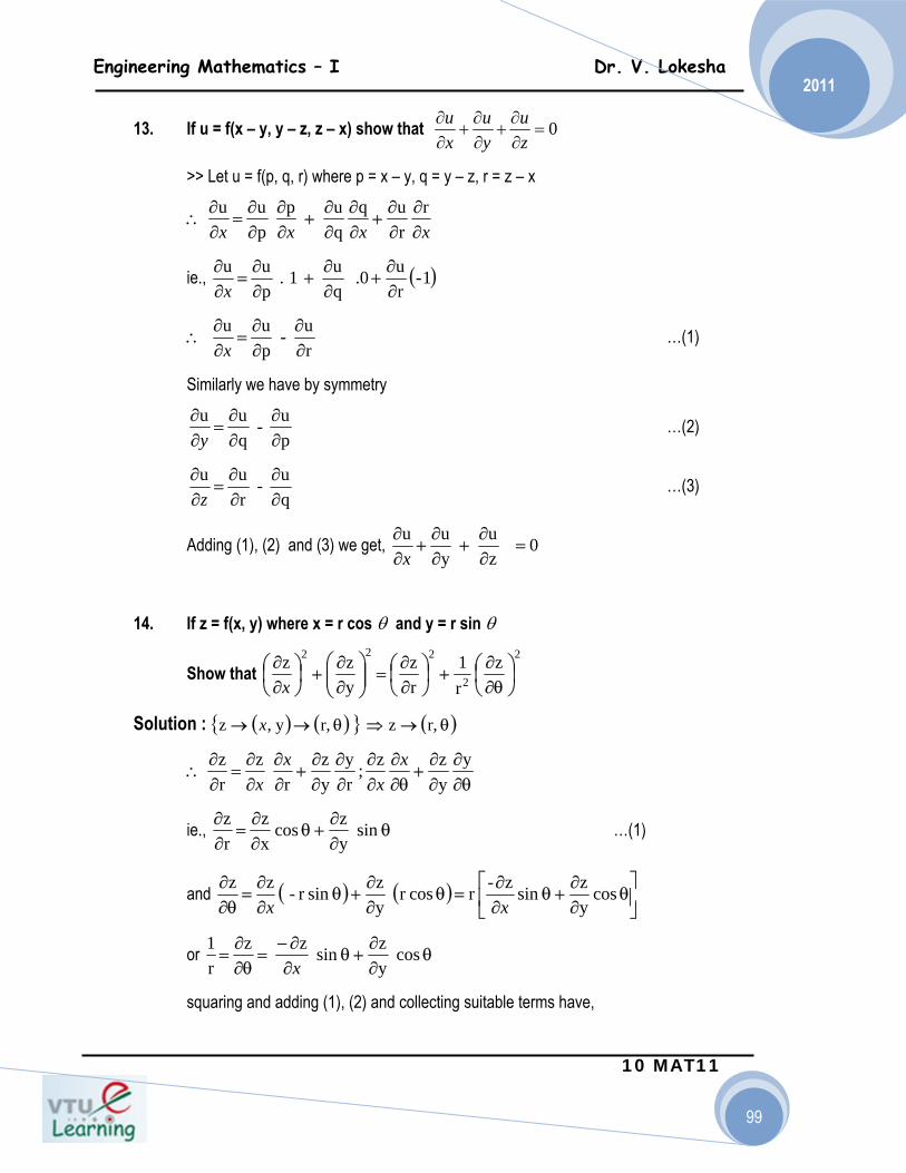
Engineering Mathematics – I Dr. V. Lokesha
10 MAT11
99
2011
13. If u = f(x – y, y – z, z – x) show that 0 =∂∂
+∂∂
+∂∂
zu
yu
xu
>> Let u = f(p, q, r) where p = x – y, q = y – z, r = z – x
xxxx ∂∂
∂∂
+∂∂
∂∂
+∂∂
∂∂
=∂∂
∴r
ru q
qu p
pu u
ie., ( )1- ru 0.
qu 1 .
pu u
∂∂
+∂∂
+∂∂
=∂∂
x
ru -
pu u
∂∂
∂∂
=∂∂
∴x
…(1)
Similarly we have by symmetry
pu -
qu u
∂∂
∂∂
=∂∂
y …(2)
qu -
ru u
∂∂
∂∂
=∂∂
z …(3)
Adding (1), (2) and (3) we get, 0 zu
yu u
=∂∂
+∂∂
+∂∂
x
14. If z = f(x, y) where x = r cos θ and y = r sin θ
Show that 2
2
222 z r1
rz
yz z
⎟⎠⎞
⎜⎝⎛
θ∂∂
+⎟⎠⎞
⎜⎝⎛
∂∂
=⎟⎟⎠
⎞⎜⎜⎝
⎛∂∂
+⎟⎠⎞
⎜⎝⎛
∂∂
x
Solution : ( ) ( ){ } ( )θ→⇒θ→→ r, z r, y ,z x
θ∂∂
∂∂
+θ∂
∂∂∂
∂∂
∂∂
+∂∂
∂∂
=∂∂
∴y
yz z ;
ry
yz
r z
rz x
xx
x
ie., θ∂∂
+θ∂∂
=∂∂ sin
yz cos
xz
rz …(1)
and ( ) ( ) ⎥⎦
⎤⎢⎣
⎡θ
∂∂
+θ∂∂
=θ∂∂
+θ∂∂
=θ∂
∂ cos yz sin z-r cosr
yz sin r - z z
xx
or θ∂∂
+θ∂∂−
=θ∂
∂= cos
yz in s z z
r1
x
squaring and adding (1), (2) and collecting suitable terms have,
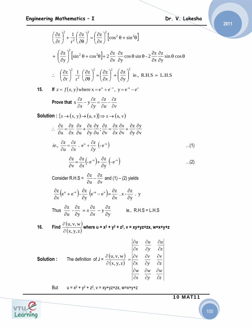
Engineering Mathematics – I Dr. V. Lokesha
10 MAT11
100
2011
[ ]θ+θ⎟⎠⎞
⎜⎝⎛
∂∂
=⎟⎠⎞
⎜⎝⎛
θ∂∂
+⎟⎠⎞
⎜⎝⎛
∂∂ 22
22
2
2
sin cos z z r1
rz
x
[ ] θθ∂∂
∂∂
θθ∂∂
∂∂
+θ+θ⎟⎟⎠
⎞⎜⎜⎝
⎛∂∂
+ cos sin yz z 2 - sin cos
yz z 2 cos sin
yz 22
2
xx
L.H.S R.H.S ie., yz z z
r1
rz
222
2
2
=⎟⎟⎠
⎞⎜⎜⎝
⎛∂∂
+⎟⎠⎞
⎜⎝⎛
∂∂
=⎟⎠⎞
⎜⎝⎛
θ∂∂
⎟⎠⎞
⎜⎝⎛
∂∂
∴x
15. If ( ) vv eexfz −=+== − -uu e y ,e x wherey ,
Prove that vz
uz
yz
xz
∂∂
−∂∂
=∂∂
−∂∂ y x
Solution : ( ) ( ){ } ( ) vu, z vu, y x, z →⇒→→
vy
yz
v z
vz ;
uy
yz
u z
uz
∂∂
∂∂
+∂∂
∂∂
=∂∂
∂∂
∂∂
+∂∂
∂∂
=∂∂
∴x
xx
x
( )u-u e- e . .,yz
xz
uzie
∂∂
+∂∂
=∂∂ …(1)
( ) ( )v-v- e- yz e- z
vz
∂∂
+∂∂
=∂∂
x …(2)
Consider R.H.S = v∂
∂−
∂∂ z uz and (1) – (2) yields
( ) ( ) y . yz - . z ee
yz - e e z vu-v-u
∂∂
∂∂
=−∂∂
+∂∂ x
xx
Thus yzy z
yz -
uz
∂∂
−∂∂
=∂∂
∂∂
xx ie., R.H.S = L.H.S
16. Find ( )( )z,y,x
w,v,u∂∂ where u = x2 + y2 + z2, v = xy+yz+zx, w=x+y+z
Solution : The definition of J = ( )( )z,y,x
w,v,u∂∂
u u ux y zv v vx y zw w wx y z
∂ ∂ ∂∂ ∂ ∂∂ ∂ ∂
=∂ ∂ ∂∂ ∂ ∂∂ ∂ ∂
But u = x2 + y2 + z2, v = xy+yz+zx, w=x+y+z

Engineering Mathematics – I Dr. V. Lokesha
10 MAT11
101
2011
Substituting for the partial derivatives we get
J = 111
xyzxzyz2y2x2
+++
Expanding by the first row, J = 2x {(x + z) – (y + x)} -2y {(y + z) – (y + x)} +2z {(y + z) – (x + z)} = 2x (z-y) – 2y(z-x) + 2z(y-x) = 2(xz – xy – yz + xy + yz – xz) = 0 Thus J = 0
17. If u = xyz , v =
yzx , w =
zxy , show that ( )
( )z,y,xw,v,u
∂∂ = 4
Solution : by data u = xyz , v =
yzx , w =
zxy
( )( )z,y,x
w,v,u∂∂ =
zw
yw
xw
zv
yv
xv
zu
yu
xu
∂∂
∂∂
∂∂
∂∂
∂∂
∂∂
∂∂
∂∂
∂∂
=
2
2
2
zxy
zx
zy
yx
yzx
yz
xy
xz
xyz
−
−
−
= ⎭⎬⎫
⎩⎨⎧
⎟⎟⎠
⎞⎜⎜⎝
⎛⎟⎠⎞
⎜⎝⎛−⎟
⎠⎞
⎜⎝⎛ −
⎟⎟⎠
⎞⎜⎜⎝
⎛ −−yx
zx
zxy
yzx
xyz
222
- ⎭⎬⎫
⎩⎨⎧
⎟⎟⎠
⎞⎜⎜⎝
⎛ −−⋅+
⎭⎬⎫
⎩⎨⎧
⋅−⎟⎟⎠
⎞⎜⎜⎝
⎛ −22 yzx
zy
zx
yz
xy
yx
zy
yzx
yz
xz
= ⎭⎬⎫
⎩⎨⎧
++⎭⎬⎫
⎩⎨⎧ −
−−
⎭⎬⎫
⎩⎨⎧
−−
yx
yx
xy
zx
zx
xz
yzx
yzx
xyz 22
2
= 0+1+1+1+1=4
Thus ( )( )z,y,x
w,v,u∂∂ = 4
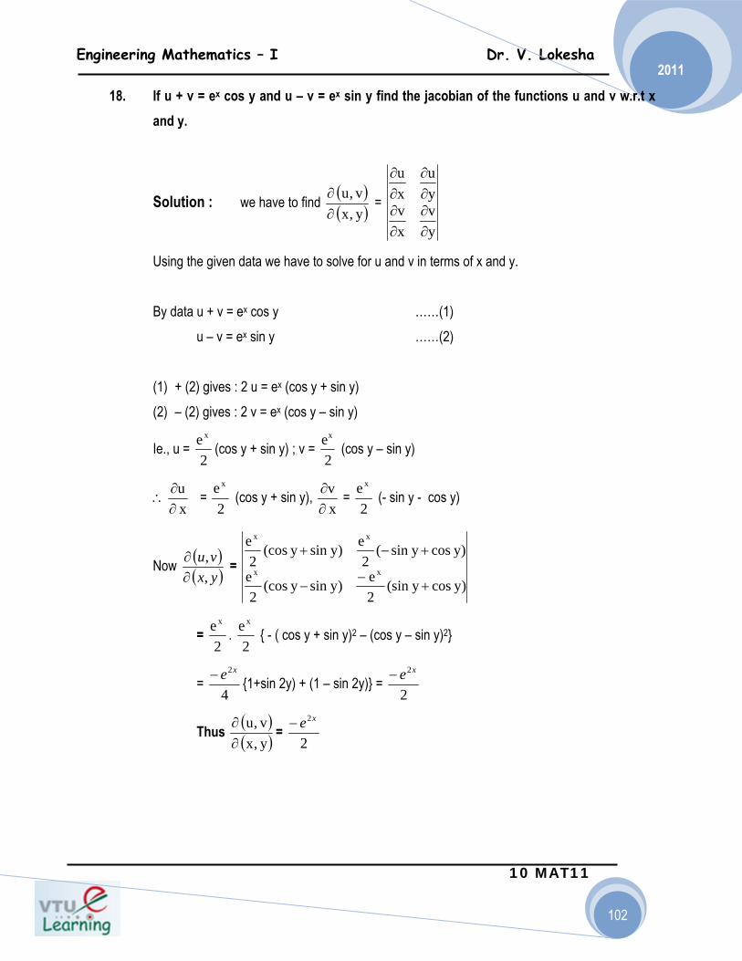
Engineering Mathematics – I Dr. V. Lokesha
10 MAT11
102
2011
18. If u + v = ex cos y and u – v = ex sin y find the jacobian of the functions u and v w.r.t x and y.
Solution : we have to find ( )( )y,x
v,u∂∂ =
yv
xv
yu
xu
∂∂
∂∂
∂∂
∂∂
Using the given data we have to solve for u and v in terms of x and y. By data u + v = ex cos y ……(1) u – v = ex sin y ……(2) (1) + (2) gives : 2 u = ex (cos y + sin y) (2) – (2) gives : 2 v = ex (cos y – sin y)
Ie., u = 2
e x
(cos y + sin y) ; v = 2ex
(cos y – sin y)
∴xu
∂∂ =
2e x
(cos y + sin y), xv
∂∂ =
2e x
(- sin y - cos y)
Now ( )( )yx
vu,,
∂∂ =
)ycosy(sin2e)ysiny(cos
2e
)ycosysin(2
e)ysiny(cos2
e
xx
xx
+−
−
+−+
= 2
e x
. 2
e x
{ - ( cos y + sin y)2 – (cos y – sin y)2}
= 4
2xe− {1+sin 2y) + (1 – sin 2y)} = 2
2xe−
Thus ( )( )y,x
v,u∂∂ =
2
2xe−
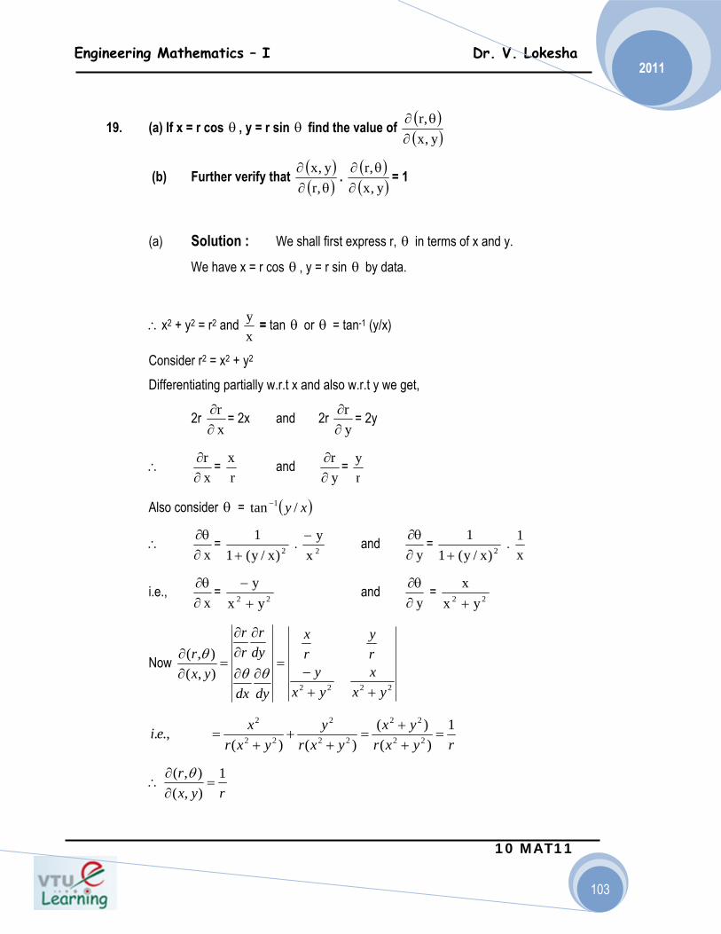
Engineering Mathematics – I Dr. V. Lokesha
10 MAT11
103
2011
19. (a) If x = r cos θ , y = r sin θ find the value of ( )( )y,x
,r∂
θ∂
(b) Further verify that ( )( )θ∂
∂,r
y,x . ( )( )y,x
,r∂
θ∂ = 1
(a) Solution : We shall first express r, θ in terms of x and y.
We have x = r cos θ , y = r sin θ by data.
∴x2 + y2 = r2 and xy = tan θ or θ = tan-1 (y/x)
Consider r2 = x2 + y2 Differentiating partially w.r.t x and also w.r.t y we get,
2r xr
∂∂ = 2x and 2r
yr
∂∂ = 2y
∴ xr
∂∂ =
rx and
yr
∂∂ =
ry
Also consider θ = ( )xy /tan 1−
∴ x∂θ∂ = 2)x/y(1
1+
. 2xy− and
y∂θ∂ = 2)x/y(1
1+
. x1
i.e., x∂θ∂ = 22 yx
y+
− and y∂θ∂ = 22 yx
x+
Now 2222
),(),(
yxx
yxy
ry
rx
dydx
dyr
rr
yxr
++−
=∂∂
∂∂∂
=∂∂
θθθ
ryxryx
yxry
yxrxei 1
)()(
)()(.,. 22
22
22
2
22
2
=++
=+
++
=
ryxr 1
),(),(
=∂∂
∴θ

Engineering Mathematics – I Dr. V. Lokesha
10 MAT11
104
2011
Solution (b) : Consider θθ sin,cos ryrx ==
rrrr
dy
ry
xrx
ryx
=+=−
=∂
∂∂
∂∂
∂∂
=∂∂ )sin(cos
cossinsincos
),(),( 22 θθ
θθθθ
θ
θθ
rr
yx=
∂∂
∴),(),(
θ
From (1) and (2) : 11
),(),(
),(),(
=⋅=∂
∂⋅
∂
∂
rr
yxr
xyx θθ
20. If ( ) uvyvux =−= ,1 then show that 1/ =JJ
Solution : uvyvux =−= );1(
uvyu
vxv
uyv
ux
=∂∂
−=∂∂
=∂∂
−=∂∂ ,),1(
uvuv
vy
uy
vx
ux
vuyxJ
−−=
∂∂
∂∂
∂∂
∂∂
=∂∂
=)1(
),(),(
uJuuvuv =∴=+−= )1(
Next we shall express u and v in terms of x and y. By data x = u - uv and y = uv
Hence .uyx =+ Also yx
yuyv
+==
Now we have, ,1,1; =∂∂
=∂∂
∴+
=+=yu
xu
yxyvyxu
Engineering Mathematics – I Dr. V. Lokesha
10 MAT11
105
2011
2)(2)(10)(
yxx
yxyyx
xv
+=
+⋅−⋅+
=∂∂
22
/
)()(
11
),(),(
yxx
yxy
yv
xv
yu
xu
yxvuJ
++−=
∂∂
∂∂
∂∂
∂∂
=∂∂
=∴
uyxyxyx
yxy
yxx 1
)(1
)()()( 222 =+
=++
=+
++
=
Thus u
J 1/ = Hence u
uJJ 1/ ⋅=⋅ Thus 1/ =JJ
21. State Taylor’s Theorem for Functions of Two Variables. Statement: Considering f (x + h, y + k) as a function of a single variable x, we have by Taylor’s Theorem
f (x + h, y + k) = f (x, y + k) + h + ---------(1)
Now expanding f (x, y + k) as function of y only,
f (x, y + k) = f (x, y) + k + --------
∴ (i) takes the form f (x + h, y + k) = f (x,y) + k +-------------------------------- +
h
+
Hence f (x + h, y + k) = f (x , y) +h
In symbol we write it as
2
22 ),(!2
),(x
kyxfhx
kyxf∂
+∂+
∂+∂
2
22 ),(!2
),(y
yxfky
yxf∂
∂+
∂∂
2
22 ),(!2
),(y
yxfky
yxf∂
∂+
∂∂
⎭⎬⎫
⎩⎨⎧
−−−−−+∂
∂+
∂∂
+∂∂
2
22 ),(!2
),(),(y
yxfky
yxfkyxfx
⎭⎬⎫
⎩⎨⎧
−−−−−−−−+∂
∂+
∂∂
yyxkyxf
xh ),(),(
!2 2
22
)1(2!2
12
22
2
2
22 −−+⎟⎟
⎠
⎞⎜⎜⎝
⎛∂∂
+∂∂
∂+
∂∂
+∂∂
+∂∂
yfk
yxfhk
xfh
yfk
xf

Engineering Mathematics – I Dr. V. Lokesha
10 MAT11
106
2011
F (x + h, y + k) = f (x,y) +
Taking x = a and y = b, (1) becomes
f (a + h, b + k) = f (a,b) + [h f x (a,b) + kf y (a,b)] + [h 2 f xx (a,b)+ 2hkf xy (a,b)
+ k 2 f yy (a,b)] + --------- Putting a + h = x and b + k = y so that h = x – a, k = y – b, we get F (x,y) = f (a,b) + [(x – a) f x (a,b) + (y – b) f y (a,b)]
= [(x – a)2 f xx (a,b) + 2 (x – a) (y – b) f xy (a,b) + (y – b)2 f yy (a,b)] +------ (2)
This is Taylor’s expansion of f (x,y) in powers of (x – a) and (y – b). It is used to expand f (x,y) in the neighborhood of (a,b) corollary, putting a = 0, b = 0 in (2), we get
f (x,y) = f (0,0) + [x f x (0,0) + y f y (0,0)] + [ x 2 f xx (0,0) + 2xy f xy (0,0)
+ y 2 f yy (0,0) ] + --------- (3) This is Maclaurin’s Expansion of f (x,y) 22. Expand e x log (1 + y) in powers of x and y up to terms of third degree. Solution: Here f (x,y) = e x log (1 + y) ∴ f (0,0) = 0 f x (x,y) = e x log (1 + y) ∴ f x (0,0) = 0
f y (x,y) = e x ∴ f y (0,0) = 1
f xx (x,y) = e x log (1 + y) ∴ f xx (0,0) = 0
f xy (x,y) = e x ∴ f xy (0,0) = 1
−−−−+⎟⎟⎠
⎞⎜⎜⎝
⎛∂∂
+∂∂
+⎟⎟⎠
⎞⎜⎜⎝
⎛∂∂
+∂∂ f
yk
xhf
yk
xh
2
!21
!21
!21
!21
y+11
y+11
Engineering Mathematics – I Dr. V. Lokesha
10 MAT11
107
2011
f yy (x,y) = - e x (1 + y) -2 ∴ f yy (0,0) = -1 f xxx (x,y) = e x log (1 + y) ∴ f xxx (0,0) = 0
f xxy (x,y) = e x ∴ f xxy (0,0) = 1
f xyy (x,y) = -e x (1 + y) 2 ∴ f xyy (0,0) = -1 f yyy (x,y) = 2e x (1 + y)-3 ∴ f yyy (0,0) = 2 Now, Maclaurin’s expansion of f (x,y) gives
f (x,y) = f (0,0) + x (f x (0,0) + y fy (0,0) + {x2 fxx (0,0) + 2xy fxy (0,0) +
y2 fyy (0,0)} + {x3 fxxx (0,0) + 3x2 y fxxy (0,0) + 3xy2 fxyy (0,0) + y3 fyyy (0,0)} + -----------
∴ex log (1 + y) = 0 + x.0 + y (1) + {x2.0 + 2xy (1) + y2 (-1)}
+ {x3.0 + 3x2y (1) + 3xy2 (-1) + y3(2)}+---------
= y + xy - y2 + (x2y = xy2) + y3 + ----------
23. Expand f (x,y) = ex Cosy by Taylor’s Theorem about the point up to the Second
degree terms.
Solution: f (x,y) = ex Cosy and a = 1, b = ∴ f = =
fx (x,y) = ex Cos y ∴ f =
fy (x,y) = -ex Sin y ∴ fy = -
fxx(x,y) = ex Cos y ∴ fxx =
fxy (x,y) = -ex Sin y ∴ fxy = -
fyy (x,y) = - ex Cos y ∴ fyy = -
Hence by Taylor’s Theorem, we obtain
y+11
!21
!21
!21
!21
21
21
21
⎟⎠⎞
⎜⎝⎛
4,1 π
4π
⎟⎠⎞
⎜⎝⎛
4,1 π
2e
⎟⎠⎞
⎜⎝⎛
4,1 π
2e
⎟⎠⎞
⎜⎝⎛
4,1 π
2e
⎟⎠⎞
⎜⎝⎛
4,1 π
2e
⎟⎠⎞
⎜⎝⎛
4,1 π
2e
⎟⎠⎞
⎜⎝⎛
4,1 π
2e

Engineering Mathematics – I Dr. V. Lokesha
10 MAT11
108
2011
f (x,y) = f + +
+ -------------
i.e., ex Cosy = + +
------------
ex Cosy = -------}
Exercise: 1) Expand exy up to Second degree terms by using Maclaurin’s theorem 2) Expand Log (1 – x – y ) up to Third degree terms by using Maclaurin’s theorem 3) Expand x2y about the point (1,-2) by Taylor’s expansion 4) Obtain the Taylor’s expansion of ex Siny about the point up to Second degree terms 5) Expand esinx up to the term containing x4
⎟⎠⎞
⎜⎝⎛
4,1 π
⎥⎦
⎤⎢⎣
⎡⎟⎠⎞
⎜⎝⎛ −+− fyyfx x 4
)1( π
!21
⎥⎥⎦
⎤
⎢⎢⎣
⎡⎟⎠⎞
⎜⎝⎛ −−+− yyx fyxfx
22
4)1(2)1( π
2e
⎥⎦
⎤⎢⎣
⎡⎟⎠
⎞⎜⎝
⎛−⎟
⎠⎞
⎜⎝⎛ −+−
242)1( eyex π
!21
+⎥⎥⎦
⎤
⎢⎢⎣
⎡⎟⎠
⎞⎜⎝
⎛ −⎟⎠⎞
⎜⎝⎛ −+⎟
⎠
⎞⎜⎝
⎛−⎟
⎠⎞
⎜⎝⎛ −−+−
2424)1(2
2)1(
22 eyeyxex ππ
2e
+⎥⎥⎦
⎤
⎢⎢⎣
⎡⎟⎠⎞
⎜⎝⎛ −−⎟
⎠⎞
⎜⎝⎛ −−−−+⎥
⎦
⎤⎢⎣
⎡⎟⎠⎞
⎜⎝⎛ −−−+
22
44)1(2)1(
!21
4)1(1 πππ yyxxyx
( )2,0 π
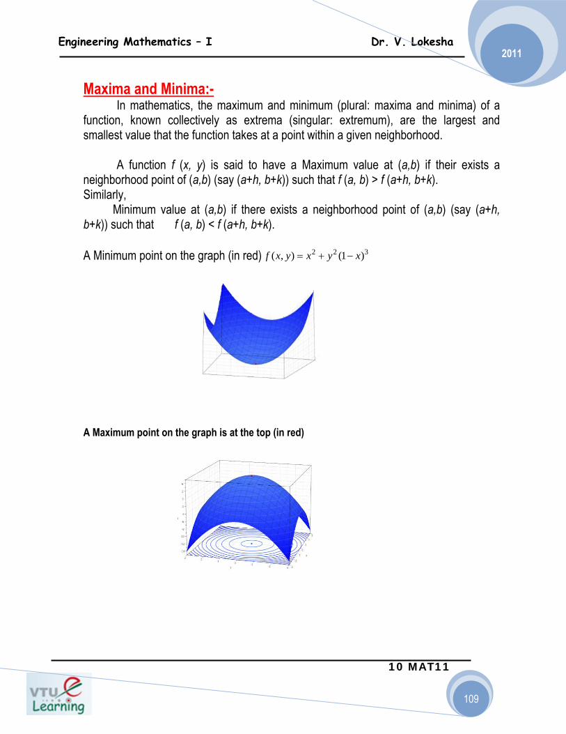
Engineering Mathematics – I Dr. V. Lokesha
10 MAT11
109
2011
Maxima and Minima:- In mathematics, the maximum and minimum (plural: maxima and minima) of a function, known collectively as extrema (singular: extremum), are the largest and smallest value that the function takes at a point within a given neighborhood. A function f (x, y) is said to have a Maximum value at (a,b) if their exists a neighborhood point of (a,b) (say (a+h, b+k)) such that f (a, b) > f (a+h, b+k). Similarly, Minimum value at (a,b) if there exists a neighborhood point of (a,b) (say (a+h, b+k)) such that f (a, b) < f (a+h, b+k). A Minimum point on the graph (in red) 2 2 3( , ) (1 )f x y x y x= + −
A Maximum point on the graph is at the top (in red)
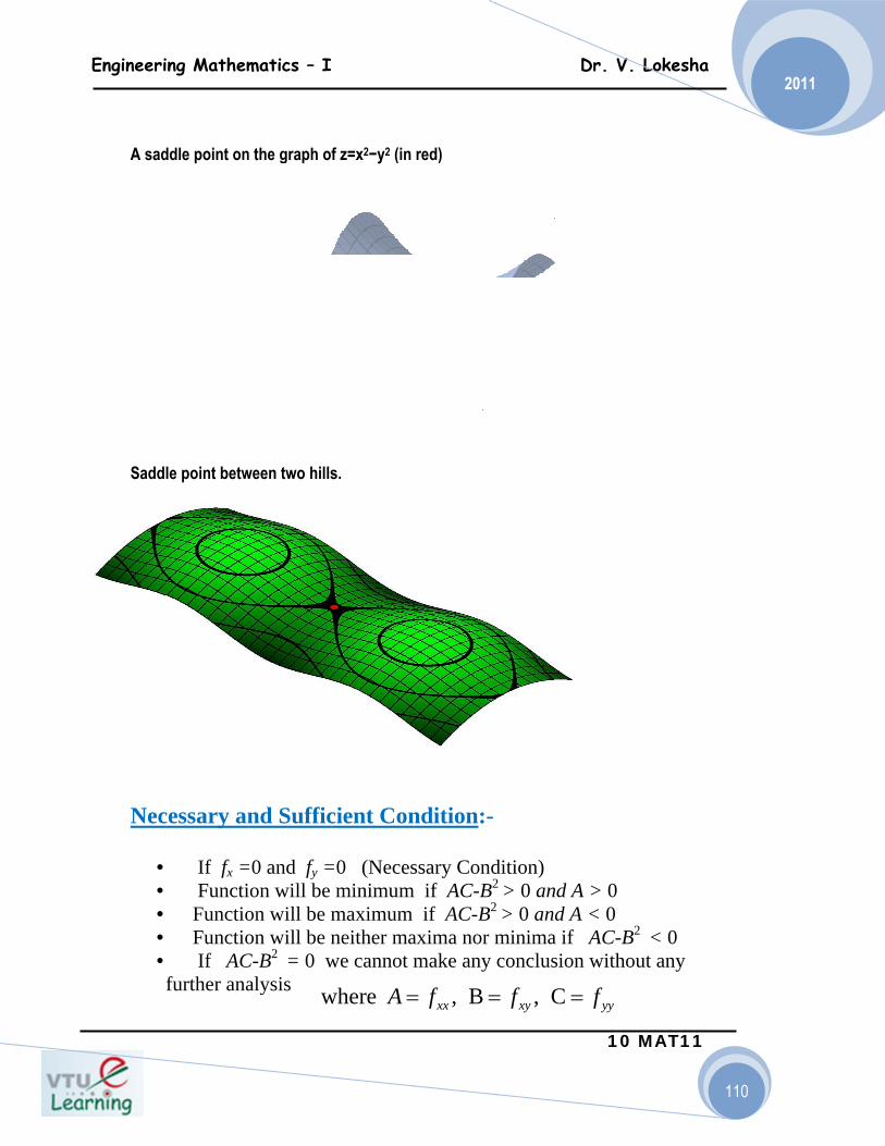
Engineeri
A sad Sadd
Nec
• • • • •
ing Mathem
ddle point on
le point betw
cessary an
If fx = Functi Functio Functio If AC
further ana
matics – I
n the graph o
ween two hills
nd Suffic
=0 and fy =ion will be on will be mon will be n
C-B2 = 0 walysis w
I
f z=x2−y2 (in
s.
cient Con
=0 (Necesminimummaximum neither ma
we cannot m
where A =
red)
ndition:-
ssary Condm if AC-B2
if AC-B2
axima nor mmake any
, Bxxf= =
dition) 2 > 0 and A > 0 and Aminima if conclusion
, Cxyf= =
Dr. V. Lo
10 MA
A > 0 A < 0
AC-B2 <n without a
yyf=
kesha
AT11
110
0 any
0
2011
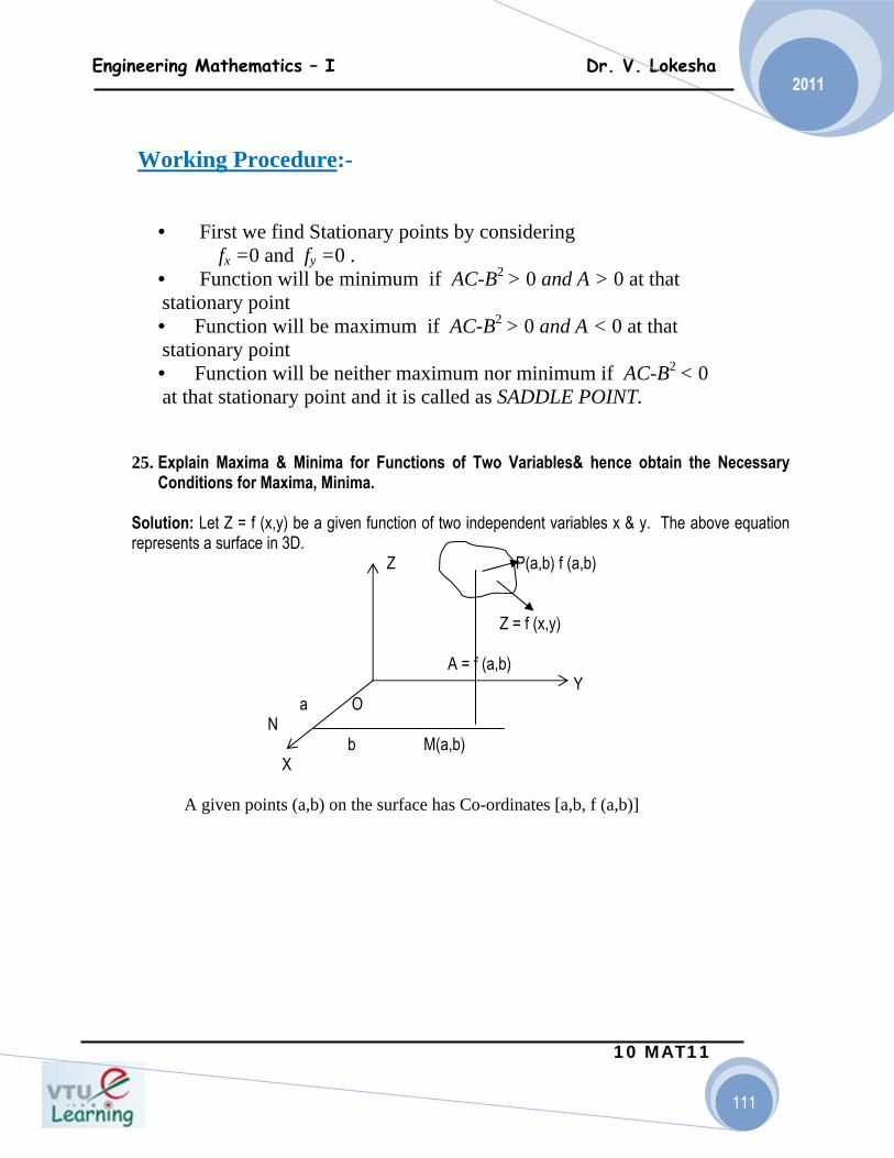
Engineering Mathematics – I Dr. V. Lokesha
10 MAT11
111
2011 Working Procedure:-
• First we find Stationary points by considering fx =0 and fy =0 .
• Function will be minimum if AC-B2 > 0 and A > 0 at that stationary point
• Function will be maximum if AC-B2 > 0 and A < 0 at that stationary point
• Function will be neither maximum nor minimum if AC-B2 < 0 at that stationary point and it is called as SADDLE POINT. 25. Explain Maxima & Minima for Functions of Two Variables& hence obtain the Necessary
Conditions for Maxima, Minima. Solution: Let Z = f (x,y) be a given function of two independent variables x & y. The above equation represents a surface in 3D. Z P(a,b) f (a,b) Z = f (x,y) A = f (a,b) Y a O N b M(a,b) X A given points (a,b) on the surface has Co-ordinates [a,b, f (a,b)]
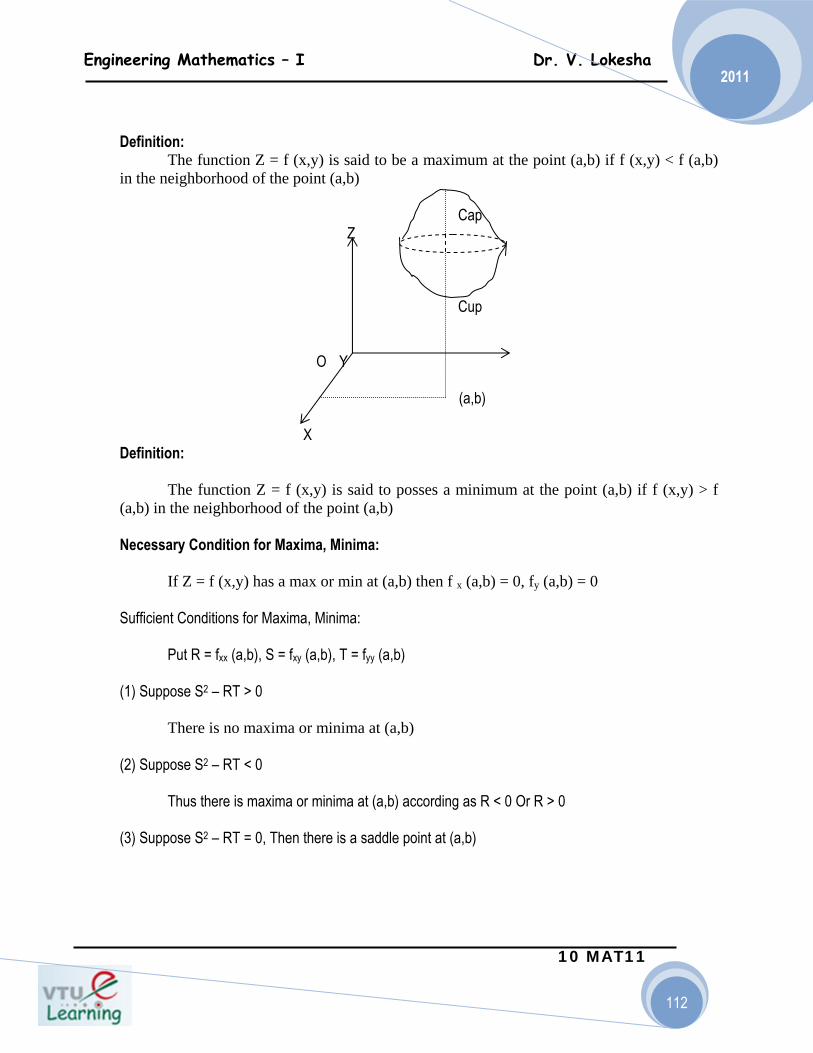
Engineering Mathematics – I Dr. V. Lokesha
10 MAT11
112
2011
Definition: The function Z = f (x,y) is said to be a maximum at the point (a,b) if f (x,y) < f (a,b) in the neighborhood of the point (a,b) Cap Z Cup O Y (a,b) X Definition: The function Z = f (x,y) is said to posses a minimum at the point (a,b) if f (x,y) > f (a,b) in the neighborhood of the point (a,b) Necessary Condition for Maxima, Minima: If Z = f (x,y) has a max or min at (a,b) then f x (a,b) = 0, fy (a,b) = 0 Sufficient Conditions for Maxima, Minima: Put R = fxx (a,b), S = fxy (a,b), T = fyy (a,b) (1) Suppose S2 – RT > 0 There is no maxima or minima at (a,b) (2) Suppose S2 – RT < 0 Thus there is maxima or minima at (a,b) according as R < 0 Or R > 0 (3) Suppose S2 – RT = 0, Then there is a saddle point at (a,b)

Engineering Mathematics – I Dr. V. Lokesha
10 MAT11
113
2011
26. Find the maxima and minima of the functions f (x,y) = x3 + y3 – 3axy, a > 0 is constant. Solution: Given f (x,y) = x3 + y3 – 3axy fx = 3x2 – 3ay, fy = 3y2 – 3ax fxx = 6x fyy = 6y. Put fx = 0, fy = 0 and solve i.e., 3x2 – 3ay = 0 & 3y2 – 3ax = 0 i.e., x2 = ay & y2 = ax
⇒ y = ∴ ⇒ = ax (∵x2 = ay)
∴ x4 = a3x i.e., x (x3 – a3) = 0 ∴ x = 0, x = a ⇒ y = 0, y = ± a ∴ The critical Or stationary points are (0,0), (a,a) and (a,-a) (1) At (0,0) R = fxx (0,0) = 0 S = fxy (0,0) = -3a T = fyy (0,0) = 0 ∴ S2 – RT = 9a2 – 0 = 9a2 > 0 ∴ There is neither a maximum or a minimum at (0,0)
ax 2 22
⎟⎟⎠
⎞⎜⎜⎝
⎛ax
axax
=∴ 2
4
Engineering Mathematics – I Dr. V. Lokesha
10 MAT11
114
2011
27. Examine the following functions for extreme values f = x4 + y4 – 2x2 + 4xy – 2y2 Solution: fx = 4x3 – 4x + 4y fy = 4y3 – 4x – 4y fxy = 4, fxx = 12 x2 – 4, fyy = 12y2 – 4 Put fx = 0, fy = 0 and solve i.e., 4x3 – 4x + 4y = 0 → (1) 4y3 + 4x – 4y = 0 → (2) Adding (1) & (2), we get 4 (x3 + y3) = 0 i.e., x3 + y3 = 0 i.e., y = - x Substitute y = -x in (1), we get 4x3 – 4x – 4x = 0 i.e., 4x3 – 8x = 0 i.e., x3 – 2x = 0 ⇒ x (x2 – 2) = 0 i.e., x = 0 & x2 – 2 =0 i.e., x = 0 & x = ± x = , - ∴x = 0, ,- and corresponding values of y are y = 0, - , ∴ The critical points are (0,0), , - , - , (1) at (0,0) R = fxx (0,0) = - 4
2
2 2
2 2 2 2
2 2 2 2
Engineering Mathematics – I Dr. V. Lokesha
10 MAT11
115
2011
S = fxy (0,0) = 4 T = fyy (0,0) = -4 ∴ S2 – RT = 16 – (-4) (-4) = 16 – 16 = 0 i.e., S2 – RT = 0, These is a saddle point at (0,0) (2) at , - R = fxx , - =24– 4 = 20 S = fxy ,- = 4 T = fyy , - = 20 ∴ S2 – RT = 16 – (20) (20) = 16 – 400 = -384 < 0 Thus these is neither maximum nor minimum according to R < 0 or R > 0 at , - Hence R = 20 > 0 ∴ There is a minimum at , - = 4 + 4 – 4 – 8 – 4 = - 8 (3) at - , R = fxx = 20 > 0 S = fxy = 4 T = fyy = 20 ∴ S2 – RT = 16 – 400 = -384 < 0
2 2
2 2
2 2
2 2
2 2
2 2
( ) ( ) ( ) ( ) ( )2244
min 222242222 −−−+−−+=∴ f
2 2
( )2,2−
( )2,2−
( )2,2−
Engineering Mathematics – I Dr. V. Lokesha
10 MAT11
116
2011
Since R > 0, ∴ There is minima at ∴ fmin = - 8 at ∴ Extreme Value = - 8 at & Exercise: 1) Find the extreme values of f = x3 y2 (1 – x – y) 2) Determine the maxima or minima of the function Sin x + Sin y + Sin (x + y) 3) Examine the function f(x,y) = 1+ sin( x2 + y2) for extremum. 28. If PV2 = K and if the relative errors in P is 0.05 and in V is 0.025 show that the error in K
is 10%.
Solution : KPV =2 by data. Also 025.0and05.0 ==VV
PP δδ
KVP loglog2log =+⇒
)(log)(log2)(log KVP δδδ =+⇒
10100)1.0(100
1.0)025.0(205.0.,.
1121.,.
=×=×∴
==+
=⋅+
KK
KKor
KKei
KK
VV
Pp
ei
δ
δδ
δδδ
Thus the error in K is 10%.
( )2,2−
( )2,2−
( )2,2− ( )2,2−
Engineering Mathematics – I Dr. V. Lokesha
10 MAT11
117
2011
29. The time T of a complete oscillation of a simple pendulum is given by the formula
⋅= glT /2π
(i) If g is a constant find the error in the calculated value of T due to an error of 3% in the value of l.
(ii) Find the maximum error in T due to possible errors upto 1% in l and 3% in g.
Solution :
( ) 2 / , Constant, 100 3
1log log 2 (log log )2
1(log ) (log 2 ) (log )2
1. ., 0 021 1100 100 (3) 1.52 2
li T l g gl
T l g
T g
T li eT lT lor
T l
δπ
π
δ δ π δ
δ δ
δ δ
= = × =
⇒ = + −
⇒ = +
= + −
⎛ ⎞× = × = =⎜ ⎟⎝ ⎠
∴ the error in T = 1.5%. (ii) If g is not a constant we have,
⎟⎟⎠
⎞⎜⎜⎝
⎛×−⎟
⎠⎞
⎜⎝⎛ ×=× 100
21100
21100
gg
ll
TT δδδ
The error in T will be maximum if the error in l is positive and the error in g is negative (or vice-versa) as the difference in errors converts in to a sum.
2)3(21)1(
21100max =−−+=⎟
⎠⎞
⎜⎝⎛ ×∴
TTδ
∴ the maximum error in T is 2%.
Engineering Mathematics – I Dr. V. Lokesha
10 MAT11
118
2011
30. The current measured by a tangent galvanometer is given by the relation
c = k tan θ where θ is the angle of deflection. Show that the relative error in c due to a
given error in θ is minimum when θ = .450
Solution : Consider c = k tan θ . K is taken as a constant.
)(tanlogloglog θ+=⇒ kc
)(tanlog)(log)(log θδδδ +=⇒ kc
δθθθδ
tansec01.,.
2
+=cc
ei
θθδθδθδθ
θθθδ
cossincos1
sincos.,. 2 =⋅=
cor
ccei
δθθ
δ2sin
2.,. =ccei
The relative error in c being cc /δ minimum when the denominator of the R.H.S. is maximum
and the maximum value of a sine function is1.
⋅==⇒=∴ 00 4590212sin θθθ or
Thus the relative error in c is minimum when 045=θ
31. 2
21 mvTIf = is the kinetic energy, find approximately the change in T as m changes
from 49 to 49.5 and v changes from 1600 to 1590. 6 Marks
Solution : We have by data 2
21 mvT = and
5.0m5.49mm,49m =δ∴=δ+=
10v1590vv,1600v −=δ∴=δ+=
Engineering Mathematics – I Dr. V. Lokesha
10 MAT11
119
2011
We have to find .Tδ (logarithm is not required)
)(21 2mvT δδ =∴
{ }2.)2(21 vmvvm δδ +
{ } 000,44,1)1600()5.0()10()1600()2()49(21,. 2 =+−=ei
Thus the change in 000,44,1−== TT δ
32. The pressure p and the volume v of a gas are concentrated by the relation
.tan4.1 tconspv = Find the percentage increase in pressure corresponding to a
diminution of ½% in volume.
Solution : 1.4 Constant ( ),pv c say= = by data.
cvp loglog4.1log =+⇒
)(log)(log4.1)(log cvp δδδ =+⇒
,21100But;04.1,. −=×=⎟
⎠⎞
⎜⎝⎛+
vv
vv
ppei δδδ by data.
7.0100or01004.1100 +=×=⎟⎠⎞
⎜⎝⎛ ×+×∴
pp
vv
pp δδδ .
Thus the percentage increase in pressure = 0.7 33. Find the percentage error in the area of an ellipse when an error of +1% is made in
measuring the major and minor axis.
Solution : For the ellipse 1// 2222 =+ byax the area (A) is given by π ab where 2a and 2b are
the lengths of the major and minor axis. Let 2a = x and 2b = y.
By data .1100,1100 =×=×yy
xx δδ
Engineering Mathematics – I Dr. V. Lokesha
10 MAT11
120
2011
xyyxabA422πππ =⋅⋅==
yxA loglog)4/(loglog ++=∴ π
)(log)(log)4/(log)(log yxA δδπδδ ++=⇒
1001001000.,. ×+×=×++=yy
xx
AAor
yy
xx
AAei δδδδδδ
211100 =+=×∴AAδ
Thus error in the area = 2% 27. If the sides and angles of a triangle ABC vary in such way that the circum radius
remains constant, prove that
0coscoscos
=++c
cB
bA
a δδδ
Solution : If the triangle ABC is inscribed in a circle of radius r and if a,b,c respectively
denotes the sides opposite to the angles A,B,C we have the sine rule (formula) given by
rC
cB
bA
a 2sinsinsin
===
or CrcBrbAra sin2,sin2,sin2 ===
)(sin2),(sin2),(sin2 CrcBrbAra δδδδδδ ===⇒
CCrcBBrbAAraei δδδδδδ cos2,cos2,cos2.,. ===
or CrC
cBrB
bArA
a δδδδδδ 2cos
,2cos
,2cos
===
Adding all these results we get,
)(2)(2coscoscos
CBArCBArC
cB
bA
a++=++=++ δδδδδδδ
But A+B+C = 180 = π radians = constant.
δδ =++⇒ )( CBA (constant) = 0
Thus 0coscoscos
=++C
cB
bA
a δδδ

Engineering Mathematics – I Dr. V. Lokesha
10 MAT11
121
2011
Multiple choice Questions:
DIFFERENTIAL CALCULUS
1) The radius of curvature at any point of catenary S=C tan Φ is a) c sec2 Φ b) c cos2 Φ c) c tan-2 Φ d)none 2) Stationary points of f(x,y) = sin x+ sin y+ sin ( x + y ) is a) (п/3, п/3) b) (п/6, п/6) c) (п/4, п/4) d) none 3) If the curvature is zero, that point is known as-------------------- a) Point of inflection b) Stationary point c) (a) or (b) d) none 4) The radius of curvature of the curve y = 4 sin x- sin 2x at x=п/2 is a) 5√5/4 b) -5√5/4 c)5√5/2 d) none 5) The function x2+2xy+ 2y2+2x+2y has a minimum value at
a) (-3/2,1/2) b)(3/2, 1/2 ) c) (3/2,-1/2) d)none 6) The stationary point of f(x,y,z)=x2+y2+z2 where x,y,z are connected by x+y+z=a is a) (a,a) b) (-a,-a) c) (2a, 0) d) none 7) The radius of curvature of the curve √x+√y =1 at the point (1/4,1/4) is ------------ a) ρ =1/√2 b) ρ=√2 c) ρ= -1/√2 d) none ) 8) The expression for the derivative of arc length in Cartesian form is given by a) ds/d�= b) ds/dx=
c) ds/dr= d) ds/dt=
9)The formulae for radius of curvature in Cartesian form is
a) ρ = (x1) 2 + (y1) 2)3/2 /x1y11+x11y1
b) ρ =
c) ρ = [(x1) 2 + (y1) 2)3/2 ]
)dr/d (r 22 θ+ 2(dy/dx)1+2d?/dr) (1+ 2(dy/dx)1+
( ) 2/3
2
211
yy+
Engineering Mathematics – I Dr. V. Lokesha
10 MAT11
122
2011 d) ρ = (1+(y1) 2 ) 3/2 10) The function for which Rolle’s theorem is true is: a) f(x)=log x in the interval [1/2,2] b) f(x)=|x+1| in the interval [-2,2] c) f(x)=| x |in the interval [-1,1] d) Non of the above 11) The value of ‘c’in Rolle’s theorem ,where and f(x)= cosx is equal to: a b) c) d)0 12).The expansion of tanx in powers of x by Maclaurin’s theorem is valid in the interval : a) b) c) d) 13) The value of ‘c’in Lagrange,s mean value theorem ,where [1,2] and f(x)= x(x-1) is : a)5/4 b)3/2 c)7/4 d) 11/6 14) The value of ‘c’in Rolle’s theorem, where [0, ] and f(x)= sinx is equal to: a) b) c) d) Non of these 15) The maximum value of logx/x is: a) 1 b)e c)2/e d) 1/e
16) The maximum value of (l/x ) x is equal to: a)e b)1 c) e 1/e d) (1/e)e
17) The difference bwtween the maximum and minimum values of the function a sinx+bcosx is: a) b) c) d) 18) Which one of the following statement is correct for the function f(x)=x3
a) f(x) has a maximum value at x=0 b) f(x) has a manimum value at x=0 c) f(x) has a neither a maximum nor a manimum value at x=0 d) f(x) has no point of inflexion 19) which one of the following is not an indeterminate form a) b) c) d)
20) In Lagrange,s mean value theorem , f1(c)= a) f(a) – f(b)/ b -a b) f(b) – f(a) / a -b c) f(b) – f(a) / b -a d) none
2/2/ ππ <<− c4/π 3/π π
( )∞∞− , ( )2/3,2/3 ππ− ( )ππ ,− ( )2/,2/ ππ−
π
6/π 3/π 2/π
222 ba + )(2 22 ba + 22 ba + 22 ba +−
∞+∞ ∞−∞ ∞∞ / ∞X0
Engineering Mathematics – I Dr. V. Lokesha
10 MAT11
123
2011
21) In Cauchy’s mean value theorem , f1(c) / g1(c) = a) f(a) – f(b)/ g(b) – g(a) b) f(b) – f(a) / g(b) – g(a) .c) f(b) +f(a) / g(b) +g(a) d) none
22) is equal to :
a) 0 b) ∞ c) log (a/b) d) log (a-b) 23) The value of is equal to:
a) -1 b) ∞ c) 1 d) 0 24) The value of (1 – cos x / 3 x2 )is equal to:
a) 3 b) 1/3 c) 1/6 d) 1/9
25) ( ex + e-x – 20) / x2 is equal to : a) 1 b) -1 c) 1/2 d) -1/2 26) The value of ( 1 + x )1/x is : a) 1 b) -1 c) 1/e d) e
27) The value of =….
a) 1 b) 2 c) 3 d)0 28) The formulae for radius of curvature in polar form is
a) ρ = rdr/dp b) ρ = [ (r 2 + (r1) 2)3/2] / [r2+2 ( r1) 2- r r2]
c) ρ =(r 2 + (r1) 2)3/2 d) None
29) The value of 1 1/x =……
a) 1 b) ∞ c) -∞ d) 0
0lim
→x x
x xb -a
0lim
→x 1log
−xx
0lim
→x
0lim
→x
0lim
→x
xx
x
sinlim0→
0lim
→x
Engineering Mathematics – I Dr. V. Lokesha
10 MAT11
124
2011
KEY ANSWERS:
1-a 2-a 3-a 4-a 5-a 6-a 7-a 8-b 9-b 10-a
11-d 12-d 13-b 14-c 15-d 16-c 17-a 18-c 19-a 20-c
21-b 22-c 23-c 24-c 25-a 26-c 27-a 28-b 29-b --