entry, exit, and differentiation in the supermarket industry · 2017-08-28 · jel classiﬁcation...

Rev Ind Organ (2011) 38:1–21DOI 10.1007/s11151-011-9278-8

Does Big Drive Out Small?Entry, Exit, and Differentiation in the Supermarket Industry

Mitsuru Igami

Published online: 5 February 2011© The Author(s) 2011. This article is published with open access at Springerlink.com

Abstract This paper measures the impact of the entry of large supermarkets onincumbents of various sizes. Contrary to the conventional notion that big stores drivesmall rivals out of the market, data from Tokyo in the 1990s show that large super-markets’ entry induces the exit of existing large and medium-size competitors, butimproves the survival rate of small supermarkets. These findings highlight the role ofstore size as an important dimension of product differentiation. Size-based entry reg-ulations would appear to protect big incumbents, at the expense of small incumbentsand potential entrants.

Keywords Deregulation · Entry and exit · Product differentiation · Retail

JEL Classification L11 · L13 · L51 · L81

1 Introduction

This paper empirically assesses the impact of large supermarkets’ entry on existingsupermarkets of various sizes. Contrary to the conventional notion that big storesdrive small rivals out of the market, the results indicate that big entrants drive out bigand medium-sized incumbents, while benefiting small stores. The outcome is consis-tent with economic theories of product differentiation; i.e., store size is providing animportant dimension to differentiate among retailers.

The deregulation of the Tokyo supermarket industry in the early 1990s provides asuitable setting to evaluate the differential impacts of large stores’ openings on existingstores. First, I analyze the incumbent stores’ responses to the entry events by ordered

M. Igami (B)UCLA Anderson School of Management, 110 Westwood Plaza C-525, Los Angeles, CA 90095, USAe-mail: [email protected]; [email protected]

123

2 M. Igami

probit regressions, where their four alternative actions are (1) exit, (2) shrink floor size,(3) stay unchanged, and (4) expand floor size. Second, since entry events are based onbig retailers’ choices of towns to enter, this prompts a concern over potential selectionbiases. I conduct a series of IV probit regressions in which I instrument the entryevents by the big entrants’ affiliations with particular geographical markets. Finally,I employ tobit regressions to analyze the magnitude of changes in floor size, usingincumbent stores’ percentage change in floor size as the dependent variable.

The results suggest that large entrants displace large and medium-size incumbents,but small supermarkets’ survival rate actually improves. Large and medium stores seemto compete directly with the new rivals, while small incumbents are insulated by prod-uct differentiation and even benefit from the positive demand externality (additionalflow of shoppers).

These findings have direct public policy implications. Regulators around the globeoften restrict the entry of large retail outlets.1 Such (anti-)competition policies areoften based on the premise that big stores drive out small ones. However, when storesize is the source of differentiation across retail services, the unintended consequencesof size-based entry regulations would appear to include: (1) softer competition amonglarge retailers, hence limited, pricier choices for consumers on a daily basis; and(2) forgone profit opportunities for small stores, who could have benefited from thepositive externalities of new big entrants.

2 Literature

This research contributes to three strands of economic literature: First, the paper offersnew empirical evidence to support economic theories of product differentiation, bycomparing the effect of large supermarkets’ entry on competing stores of varioussizes. D’Aspremont et al. (1979), Shaked and Sutton (1982), and Perloff and Salop(1985) showed that product differentiation could soften price competition.2 However,as Borenstein and Netz (1999) noted, theoretical work on product differentiation hasproduced few corresponding empirical studies. I examine a particular type of productdifferentiation in the retail industry: store size. The results highlight the role of productdifferentiation in relaxing competition. More specifically, this study supports the the-oretical prediction by Zhu et al. (2006) that the tradeoff between the business-stealingeffect and the positive demand externality depends on the degree of differentiationbetween the entrant and the incumbents.

1 Zoning laws in Britain, France, Germany, India, Japan, Korea, and Poland restrict the development oflarge stores (Lewis 2004). Even in the United States, state and local authorities and state courts often makethe final decisions on whether to allow the entry of a new Wal-Mart store (Sobel and Dean 2008).2 Theoretical predictions vary with respect to the extent of differentiation. For example, D’Aspremontet al. (1979) show that, in order to soften price competition, two firms would maximally differentiate ona Hotelling product line. Neven and Thisse (1990) and Irmen and Thisse (1998) extend this frameworkto competition over multiple product attributes. In contrast, Anderson et al. (1992) show that firms thatcompete in two dimensions may locate together at the center of the market under certain conditions. Still,the basic insight remains the same: Differentiation opens the possibility for softening competition.

123

Does Big Drive Out Small? 3

Second, this paper augments the empirical work on entry and exit, by introducingthe product-differentiation aspect to the analysis in two ways: by examining the dif-ferential impacts of entry on the exit rates of the incumbents of different sizes; and byanalyzing the incumbents’ responses in terms of store-size changes. It is only recentlythat the economics of product differentiation has been studied explicitly in conjunc-tion with entry and exit. Mazzeo (2002) uses a static framework, while Ellickson(2007) uses a dynamic structure. This paper takes an alternative approach to capturethe dynamics of the phenomena, by exploiting exogenous regulatory changes andstudying incumbents’ responses to the entry of bigger stores.

Third, this paper sheds new light on the economic analysis of the “Wal-Mart effects;”i.e., inquiries into the competitive effects of big entrants on incumbents, by introducingthe viewpoint of product differentiation. Shoppers world-wide have witnessed the riseof big retailers, such as Wal-Mart and Carrefour. The proliferation of these large storeshas stirred the debate over the consequences of their entry into local markets. Someanalysts credit them with lowering prices, raising productivity, and making wider prod-uct variety available (Hausman and Leibtag 2007; Basker 2005); others blame themfor destroying jobs and local businesses (Wal-Mart Watch 2005). Basker’s (2007) sur-vey summarizes the discoveries to date and concludes that incumbents’ exit due toWal-Mart range between two to five stores at a county level. Detailed panel data ofsupermarkets at a sub-county level allow me to address this issue while mitigatingconcerns over spurious correlations.3

3 Industry and Data

The supermarket industry in Tokyo in the early 1990s provides a suitable testing groundfor evaluating the impact of large stores’ openings on incumbents’ exit rates for threereasons: First, stores of various sizes compete in this sector, offering a laboratoryto analyze the differential impacts of large entrants on incumbent stores of differentsizes. Second, it is relatively easy to identify local markets geographically. Unlikeshopping for, say, fashion apparel or consumer electronics, which tends to cluster inurban centers, shoppers stay close to their home as far as the day-to-day purchase offood staples is concerned. Third, the (exogenous) relaxation of entry regulations in1990 allows me to identify the impact of large stores’ entry by comparing the exitrates of incumbent supermarkets in similar towns with and without an entry event.

3.1 Definition of Supermarket

This study follows the industry standard in defining a supermarket as: (1) a self-service store, with (2) floor space of at least 231 m2(2, 486 ft2) and/or minimum annual

3 County-level observations may mask the rise and fall of towns; therefore using sub-county-level dataincreases the relevance of empirical analysis to actual shopping behavior and competition. Additionally,stores often change their size over time. If, for instance, a small store expands its floor area, a simple censusmight count it as a small store exit and, simultaneously, a medium store entry as if the latter drove out theformer. Panel data are a convenient way to capture actual exit patterns.

123

4 M. Igami

revenue of �100 million ($1 million), and with (3) over 30% of revenue from foodproducts including (but not limited to) fish, meats, and vegetables.4 My data on super-markets—based on the Shogyokai’s (1990 & 1995) trade press Japan SupermarketDirectory—contain retail establishments satisfying these conditions.5

Practical meanings of the definition will be clearer in comparison with other retailformats. Conditions (1) and (2) distinguish supermarkets from more traditional spe-cialty shops that sell fish, meats, or vegetables, which typically offer customizedservices and are smaller in size. Additionally, condition (3) ensures that a supermar-ket is an outlet primarily for the retailing of food, as distinguished from conveniencestores, drug stores, tobacco shops, or department stores. More recently, a larger super-market with a wider lineup of household merchandise is often called a GMS (generalmerchandise store), hypermart, or superstore. The industry standard does not excludethese types of supermarkets from the definition; neither does this paper.6 Hence thelikes of Aeon, Daiei, or Seiyu (the Japanese equivalent to Wal-Mart, Tesco, Carrefour,or Metro) are incorporated in the subsequent empirical analysis.

3.2 Train Station-Centered Geographical Markets

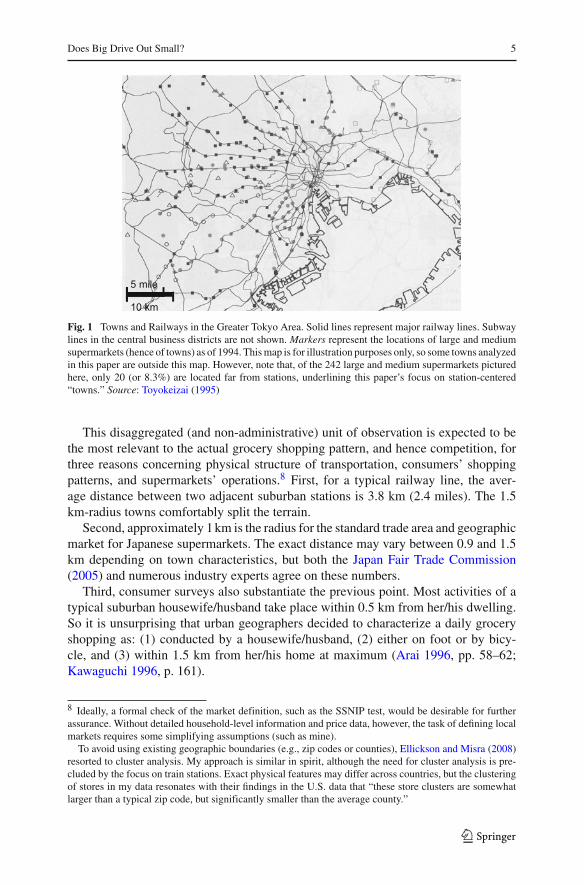
In the suburbs of the Greater Tokyo region (which spans Tokyo, Kanagawa,Saitama, and Chiba prefectures), relevant geographical markets can be identified bytrain stations along major railways (Fig. 1). This is because daily shopping activities insuburban Tokyo are concentrated around train stations. Since trains are the predomi-nant means of transport for commuters, stations provide focal points for both shoppersand retailers (Kawaguchi 1996, p. 175).

Note that 91.7% of the supermarkets shown in Fig. 1 are located within 1.5 km froma station. Hence, the market database from Toyokeizai’s (a private business press andthink tank) Metropolitan Commercial Map 1995 compiles demographic and retail-related information by 240 suburban “towns” along major railway lines in the region.7

Each “town” contains a geographical area within a radius of approximately 1.5 km(0.93 mile) from the train station.

4 This (establishment level) definition of a supermarket is analogous to the one used in the U.S.: “a storeselling a full line of food products and generating at least $2 million in yearly revenues” (Ellickson 2007,p. 48).5 For each store, the directory lists its name, street address, year of opening, operating firm, location type,building structure, parking capacity, gross revenue, types of merchandise sold, floor area, rented area, andthe number of employees.6 This is also the convention in the U.S. supermarket industry (Ellickson 2007).7 Metropolitan Commercial Map 1995 contains a number of localities that are better characterized as cen-tral business districts rather than suburban residential areas. Hence I drop 29 local markets in which thenumber of regular commuters exceeds that of residents. I also drop one locality in which the train stationwas established only after 1990. Finally, I drop four towns for which the data on train users are unavailable,and another four towns for which exit rates are not available. All of this leaves 202 towns.

The listed variables include population, the number of households and commuters, the principal meansof transport between residence and the nearest train station, commercial land price, the number of retailshops, and their aggregate floor space and revenue as of 1991. In addition, the growth rate between 1984and 1989 of the number of regular commuters is taken from the Institution for Transport Policy Studies’annual survey (1986 and 1991 issues), directed by the Ministry of Transport.

123


Fig. 1 Towns and Railways in the Greater Tokyo Area. Solid lines represent major railway lines. Subwaylines in the central business districts are not shown. Markers represent the locations of large and mediumsupermarkets (hence of towns) as of 1994. This map is for illustration purposes only, so some towns analyzedin this paper are outside this map. However, note that, of the 242 large and medium supermarkets picturedhere, only 20 (or 8.3%) are located far from stations, underlining this paper’s focus on station-centered“towns.” Source: Toyokeizai (1995)

This disaggregated (and non-administrative) unit of observation is expected to bethe most relevant to the actual grocery shopping pattern, and hence competition, forthree reasons concerning physical structure of transportation, consumers’ shoppingpatterns, and supermarkets’ operations.8 First, for a typical railway line, the aver-age distance between two adjacent suburban stations is 3.8 km (2.4 miles). The 1.5km-radius towns comfortably split the terrain.

Second, approximately 1 km is the radius for the standard trade area and geographicmarket for Japanese supermarkets. The exact distance may vary between 0.9 and 1.5km depending on town characteristics, but both the Japan Fair Trade Commission(2005) and numerous industry experts agree on these numbers.

Third, consumer surveys also substantiate the previous point. Most activities of atypical suburban housewife/husband take place within 0.5 km from her/his dwelling.So it is unsurprising that urban geographers decided to characterize a daily groceryshopping as: (1) conducted by a housewife/husband, (2) either on foot or by bicy-cle, and (3) within 1.5 km from her/his home at maximum (Arai 1996, pp. 58–62;Kawaguchi 1996, p. 161).

8 Ideally, a formal check of the market definition, such as the SSNIP test, would be desirable for furtherassurance. Without detailed household-level information and price data, however, the task of defining localmarkets requires some simplifying assumptions (such as mine).

To avoid using existing geographic boundaries (e.g., zip codes or counties), Ellickson and Misra (2008)resorted to cluster analysis. My approach is similar in spirit, although the need for cluster analysis is pre-cluded by the focus on train stations. Exact physical features may differ across countries, but the clusteringof stores in my data resonates with their findings in the U.S. data that “these store clusters are somewhatlarger than a typical zip code, but significantly smaller than the average county.”

123

6 M. Igami

0

100

200

300

400

500

1955 1960 1965 1970 1975 1980 1985 1990 1995 2000

(store)

Fig. 2 Number of supermarket openings. Note: The number for the year 1955 includes those stores thatopened before 1955. Source: (Minakata 2004, Tables 1–3, p. 16)

3.3 The 1990 Deregulation and Its Historical Context

A priori, there are no natural classification criteria for the sizes of retail outlets. Inthe regulatory context of the Japanese retail sector, however, a suitable categorizationarises from the laws that define large, medium, and small stores. The Large-scale RetailLaw, introduced in March 1974, sought to cap the new openings of any retail storewith floor space 1, 500 m2(16, 146 ft2) and up.9 Later, the 1979 revision of the lawfurther added another target category: stores with 500–1,499 m2 (5,382–16,145 ft2).This paper defines stores with floor space of 1, 500 m2 and above, 500–1,499 m2, andless than 500 m2 as “large,” “medium,” and “small,” respectively, because these arethe size categories that had defined the evolution of the sector.10

The new entry of supermarkets was particularly hindered during the 1980s. TheMinistry of International Trade and Industry (MITI) tightened the enforcement of theregulations in October 1981, publicly dissuading retailers from opening new largestores. Consequently, only small supermarkets could open during this period (Fig. 2:the period marked by “1” ).

In May 1990, however, some of the prohibitive conditions in the Large-scale RetailLaw were relaxed, which prompted a boom of new large outlets. The regulators beganto accept all of the entry requests, regardless of store sizes, and abolished so-called“entry control areas” that were previously untouchable for newcomers. The driving

9 This was not the first time that government regulations targeted larger stores. Since the inception ofdepartment stores a century ago, various forms of legal entry barriers existed in Japan. The first was theDepartment Store Law, introduced in the 1930s in response to conventional retailers’ political activism.The law targeted nascent department stores and restricted their entry and operation. See Minakata (2004)for the industry context.10 Although the threshold for being “large” (1, 500 m2) is relatively low by international comparison, theactual size of the large entrants in my study (4, 992 m2, or 53, 716 ft2, on average) is comparable to thoseof major supermarkets in other countries including the U.K., where the average store size of supermarketchains range between 5,800 and 45, 200 ft2 (Smith 2004).

123


force behind this policy shift was the pressure from the U.S. government to “liberalize”Japan’s domestic markets during the trade talks in the late 1980s. One can thereforeregard this entry deregulation as an exogenous change in the industry environment.11

This study focuses on the years immediately after the deregulation (Fig. 2: the periodmarked by “2” ) in order to avoid confounding the effects from the subsequent wavesof deregulation.

The exogenous change in regulatory policies allows me to address the timing of bigretailers’ entry. To capture the changes following the 1990 deregulation, I employ the1990 and 1995 editions of Japan Supermarket Directory, which list the store infor-mation as of September 1989 and 1994. This sample period gives a sufficient timeinterval for observing new entries and incumbents’ responses, which typically take atleast a year or two, while limiting the risk of confounding the effects of various policychanges in the late 1990s.12 Moreover, five years would allow big retailers to opensome outlets but not in all the promising towns, mainly because of the illiquid natureof markets for huge properties and credit constraints. The resulting variation acrosstowns allows me to identify the impact.

3.4 Descriptive Statistics of Towns and Supermarkets

From these two sets of data, I reconstruct the market configuration for each of the202 localities, by connecting stores’ street addresses to those corresponding to towns.Table 1 presents summary statistics.

The average town counts 88,957 residents. Tokyo is comparable to other urban areasin terms of population density. With 4,430 people per km2, it ranks as mere number128 among the world’s 189 major urban areas.13 Prominent European cities such asMadrid (5, 680/km2), Athens (5, 500/km2), London (5, 290/km2), and Barcelona(5, 210/km2) surpass Tokyo. In short, Tokyo is not Hong Kong (25, 740/km2).

The growth potential of demand is proxied by the growth rate between 1984 and1989 of the number of “regular commuters,”14 the sample mean of which is 16.4%.There are on average 1,162 retail shops of all categories, with total floor space of72, 800 m2 (783, 619 ft2). I intend to measure the “depth” of demand by total retailrevenue per capita (which averaged �1.35 million, or $13,500), which reflects theextent of shoppers from outside the town and other household characteristics such asincome and taste. In 1989, a typical local market had 1.50 small, 1.77 medium, and1.25 large food supermarkets.

11 Even if the Japanese retailers had exercised considerable bargaining power over the timing and the extentof the entry deregulation, the analysis and conclusion of this paper would remain unchanged. In that case,the results would actually underestimate the true impact of new entry because the incumbents, who were ina position to influence the policy change, should have been better prepared than otherwise for the intensifiedcompetition from new entrants. This direction of bias would not favor my result.12 An “entry” is the opening for business in my data set. The majority of the entries occurred in the firsthalf of the 1990–1994 interval. The latest entry events occurred in April 1994. I confirmed that droppingthe two towns (out of 27) that experienced entries in 1994 does not alter the results materially.13 Wikipedia, accessed on August 13, 2009.14 Train users with fixed-route commutation tickets for one month or longer (teiki-ken).

123

8 M. Igami

Table 1 Summary statistics for town characteristics

Variable Observation Mean Standarddeviation

Minimum Maximum

Population growth rate (%) 202 16.4 20.6 -15.6 135.5

Population 202 88,957 33,956 13,766 182,590

Retail revenue per capita (mn yen) 202 1.35 0.96 0.22 9.56

Num. retail shops 202 1,162 758 197 4,704

Retail floor area (m2) 202 72,800 46,385 10,471 345,600

Num. incumbents: large 202 1.25 1.13 0.00 6.00

Num. incumbents: medium 202 1.77 1.35 0.00 6.00

Num. incumbents: small 202 1.50 1.48 0.00 6.00

Following the regulatory thresholds, store size categories are defined based on floor area (Small: 1–499 m2,medium: 500–1,499 m2, and large: 1,500 m2 or larger)

The outcome variable of interest is the incumbent supermarkets’ responses between1989 and 1994: exit, shrink, stay unchanged, or expand. Table 2 displays the store-leveldescriptive statistics.

Out of the 912 incumbent supermarkets in 1989, 94 exited, leaving 818 stores in1994. Those who survived expanded their floor size by 2.9% on average. There were252 large, 358 medium, and 302 small incumbents in 1989. Across all stores, 10%exited, 15% expanded, and 10% shrank their floor sizes (“stay unchanged” is theomitted category that accounts for the remaining 65%). These percentages do not varymuch by size although small stores are slightly more likely to exit (16%).

4 Empirical Analysis

This section presents the findings from three sets of empirical analyses: (1) orderedprobit regressions of incumbents’ decisions to exit, shrink, stay unchanged, or expand(Sect. 4.1); (2) the set of similar (binary) probit regressions with geographical instru-ments for big entrants’ town choice (Sect. 4.2); and (3) tobit regressions of incumbents’change in floor space (Sect. 4.3).

In all of the specifications, the identification of the entry effects on incumbentsrelies on the following two features of the study. First, the framework assumes inde-pendent local markets in which the following three events occur: (1) The incumbentsupermarkets of various sizes, without knowledge of the entry deregulation, operatefrom before 1990;15 (2) Upon the deregulation in 1990, the potential (big) entrantsobserve the existing store configuration in all local markets and choose towns to enter;and (3) The incumbents observe the actual entrants and decide by 1994 whether tocontinue in business (and if so, whether to change own store size). These timing and

15 It is reasonable to assume a lack of anticipation because most incumbents had opened by the mid 1980s,long before the U.S.-Japan trade talks started discussing the retail deregulation.

123


Table 2 Summary statistics for store-level observations

Variable Observation Mean Standarddeviation

Minimum Maximum

1. All incumbent stores

Floor Size in 1989 (m2) 912 1,908 3,078 57 27,413

Floor Size in 1994 (m2) 818 2,024 3,221 62 27,413

Change in floor size (%) 818 2.9 29.4 −74.7 53.2

Indicator: Exit 912 .10 .30 0 1

Indicator: Expansion 912 .15 .36 0 1

Indicator: Shrinkage 912 .10 .30 0 1

Indicator: treatment (Large Entrant) 912 .11 .31 0 1

2. Large incumbent stores

Floor size in 1989 (m2) 252 5,199 4,350 1,508 27,413

Floor size in 1994 (m2) 236 5,332 4,488 735 27,413

Change in floor size (%) 236 −0.3 16.3 −74.7 179.0

Indicator: exit 252 .06 .24 0 1

Indicator: expansion 252 .19 .39 0 1

Indicator: shrinkage 252 .12 .32 0 1

Indicator: treatment (large entrant) 252 .11 .31 0 1

3. Medium incumbent stores

Floor size in 1989 (m2) 358 948 306 500 1,499

Floor size in 1994 (m2) 328 969 383 390 3,800






4. Small incumbent stores

Floor size in 1989 (m2) 302 300 135 57 499

Floor size in 1994 (m2) 254 313 141 62 895






Following the regulatory thresholds, store size categories are defined based on floor area (Small: 1–499 m2,medium: 500–1,499 m2, and large: 1,500 m2 or larger)

informational assumptions are motivated by the historical/institutional background ofthe industry (see Sect. 3).

Second, the data set contains observations of similar towns (and individual storeswithin each of them) with and without entry events, both before (1989) and after

123

10 M. Igami

Table 3 Ordered probit regressions of decision to Exit < Shrink < Unchanged < Expand

Dep. var.: Decision to Exit < Shrink < Stay Unchanged < Expand

(1) (2) (3)

Treated: large 0.03 (.30) −0.82 (.46)* −0.73 (.47)

Treated: medium −0.56 (.20)*** −0.74 (.22)*** −0.79 (.22)***

Treated: small 0.28 (.17)* 0.23 (.16) 0.22 (.20)

Treated * floor 1.69e−4 (0.81e−4)** 1.49e−4 (0.80e−4)*

Floor 1.28e−5 (1.4e−5) 1.44e−5 (1.48e−5)

Large 0.29 (.10)*** 0.23 (.13)* 0.23 (.13)*

Medium 0.23 (.10)** 0.22 (.10)** 0.22 (.10)**

Constant (=Small) – – –

Controls No No Yes

Instruments No No No

Observations 912 912 912

Pseudo R2 .01 .01 .02

Standard errors (clustered by 202 towns) in parentheses; * significant at 10%; ** significant at 5%;*** significant at 1%

(1994) the entry deregulation. This variation in data, together with the institutionalbackground, allows me to identify the impact of big entrants on existing supermarkets.

4.1 Ordered Probit: Exit, Shrink, Stay Unchanged, or Expand

The first set of results is based on ordered probit regressions (Table 3). The dependentvariable is the four discrete alternatives for an incumbent: (1) exit; (2) stay and shrink;(3) stay unchanged; or (4) stay and expand, ordered in this manner.

Formally, store i’s observed choice is

yi =

⎧⎪⎪⎨

⎪⎪⎩

exit if y∗i ≤ c1

shrink size if c1 < y∗i ≤ c2

stay unchanged if c2 < y∗i ≤ c3

expand size if c3 < y∗i ,

(1)

where c1, c2, and c3 are threshold parameters. I specify the latent variable y∗i repre-

senting incumbent supermarket i’s profit as

y∗i = αSIZEi + βSIZEi Di + Xiγ + εi , (2)

where Di is the dummy variable that indicates the entry of a new big supermarket(“treatment” ) in the town in which store i operates.

The vector Xi includes the following town characteristics: Population growth ratebetween 1984 and 1989, Population, Retail revenue per capita, the Number of retailshops (of any kind), and Retail floor area, (i.e., the town’s total floor space that was

123


dedicated to retail trade).16 It also incorporates the number of existing rival supermar-kets in the town as of summer 1989, specified as a linear combination of the numbersof large, medium, and small incumbents, and their squared terms.17 The error term εi

is i.i.d. standard normal.Large, medium, and small incumbents may have different intercepts, αSI Z Ei , where

SI Z Ei ∈ {large, medium, small}, with small as the omitted category. The coeffi-cients of interest are the effects of new entry, βSI Z Ei , which are also allowed to varyby size classes of incumbents.18

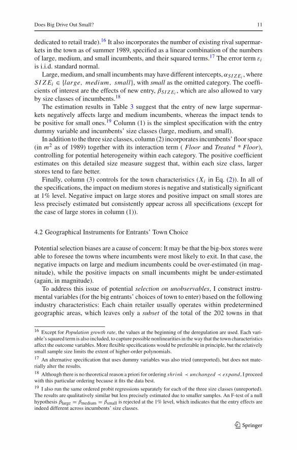
The estimation results in Table 3 suggest that the entry of new large supermar-kets negatively affects large and medium incumbents, whereas the impact tends tobe positive for small ones.19 Column (1) is the simplest specification with the entrydummy variable and incumbents’ size classes (large, medium, and small).

In addition to the three size classes, column (2) incorporates incumbents’ floor space(in m2 as of 1989) together with its interaction term ( Floor and Treated * Floor),controlling for potential heterogeneity within each category. The positive coefficientestimates on this detailed size measure suggest that, within each size class, largerstores tend to fare better.

Finally, column (3) controls for the town characteristics (Xi in Eq. (2)). In all ofthe specifications, the impact on medium stores is negative and statistically significantat 1% level. Negative impact on large stores and positive impact on small stores areless precisely estimated but consistently appear across all specifications (except forthe case of large stores in column (1)).

4.2 Geographical Instruments for Entrants’ Town Choice

Potential selection biases are a cause of concern: It may be that the big-box stores wereable to foresee the towns where incumbents were most likely to exit. In that case, thenegative impacts on large and medium incumbents could be over-estimated (in mag-nitude), while the positive impacts on small incumbents might be under-estimated(again, in magnitude).

To address this issue of potential selection on unobservables, I construct instru-mental variables (for the big entrants’ choices of town to enter) based on the followingindustry characteristics: Each chain retailer usually operates within predeterminedgeographic areas, which leaves only a subset of the total of the 202 towns in that

16 Except for Population growth rate, the values at the beginning of the deregulation are used. Each vari-able’s squared term is also included, to capture possible nonlinearities in the way that the town characteristicsaffect the outcome variables. More flexible specifications would be preferable in principle, but the relativelysmall sample size limits the extent of higher-order polynomials.17 An alternative specification that uses dummy variables was also tried (unreported), but does not mate-rially alter the results.18 Although there is no theoretical reason a priori for ordering shrink ≺ unchanged ≺ expand, I proceedwith this particular ordering because it fits the data best.19 I also run the same ordered probit regressions separately for each of the three size classes (unreported).The results are qualitatively similar but less precisely estimated due to smaller samples. An F-test of a nullhypothesis βlarge = βmedium = βsmall is rejected at the 1% level, which indicates that the entry effects areindeed different across incumbents’ size classes.

123

12 M. Igami

firm’s choice set for entry. In particular, two different urban structures are relevant:(1) railway lines; and (2) prefectures.

Regarding railways, many of the major retailers are closely affiliated with particularrailway lines and their train operators. Some retailers are the grocery-store divisionsof the conglomerates that also own and operate railway and property businesses.20

The institutional context is as follows: First, the railway transport enterprise involvesmassive property investment, in both land strips beneath railroads and train stationstructures. Second, over time, the train operators diversified into real estate broker-age/development activities and retail services due to strong complementarities thatsurround property deals. Third, since location is central to successful retail services,major retailers either are engaged in close connections with railway/property conglom-erates or are parts of such entities themselves. It is therefore not surprising that thechain operators tend to open big stores along their affiliated railway lines, exploitinginformational advantages in local real estate markets.21

With respect to prefectures, a chain retailer is often rooted in a certain prefecture as amatter of geographic origin. In addition to the informational advantages in local prop-erty markets, geographic familiarity brings two benefits. First, geographical proximityto its supplier/distribution networks facilitates the arrangement of logistics. Second,the familiarity with local rules (such as ordinances) ensures low probabilities of legaland/or political disruptions in opening new big stores. Therefore, the propensity ofentry is higher when a town belongs to a major retailer’s prefecture of origin.22

I identify each big retailer’s geographic specialization from the Appendices of theMetropolitan Commercial Map (Toyokeizai 1995) and various issues of Large-scaleRetail Shops Directory (an annual publication also from Toyokeizai). Two sets of IVsare constructed: (IV-1) the number of big retail firms that operate along each railwayline, and prefecture dummy variables; and (IV-2) the same railway-based IVs, and thenumber of big retail firms that operate from each prefecture.

Due to the institutional background in the above, a potential entrant enjoys sig-nificant informational and cost advantages when opening a new store in its familiargeographic areas (either along specific railway lines, in certain prefectures, or both).23

Thus, towns that happen to be located in the “backyards” of many big-box operators(i.e., towns that are located along railway lines and prefectures that are home to manybig retailers) are more likely to experience entry events, for economic mechanisms

20 Examples include Odakyu, Keio, Tokyu, Keikyu, Seibu, and Tobu. See Masuda (2002) for the historicalbackground on the railway networks and urban development in Tokyo.21 This advantage of an entrant is uncorrelated with incumbents’ decisions to exit or change floor sizebecause it is a strictly private benefit. Let us also note that such an informational clout does not translateinto an entrant’s ability to “kick out” incumbents (by means other than product-market competition). SeeMasuda (2002) for the close interaction between the railway transport, real estate, and retail businesses.22 This instrumentation strategy is similar in spirit to the one employed in the Wal-Mart literature: A loca-tion’s physical distance from the company’s headquarter in Bentonville, Arkansas, predicts the likelihoodand timing of new store openings in that town (see Basker 2007).23 See Sect. 3 for the details of the urban structure in the Greater Tokyo region. One rationale for such localspecializations and informational advantages is the illiquid nature of markets for huge properties, whichcreates an environment characterized by imperfect information.

123


that are unrelated to the likelihood of incumbents’ exit or expansion (i.e., the outcomevariables of interest).

Table 4 shows the results of binary IV-probit regressions. Ordered IV-probit regres-sions may achieve higher efficiency, in principle, but the actual estimation wouldbecome computationally expensive. As a logically consistent alternative method, Iconduct three binary IV-probit regressions that divide an incumbent’s four choicesdifferently: (Panel-A) “exit” or “shrink/unchanged/expand;” (Panel-B) “exit/shrink”or “unchanged/expand;” and (Panel-C) “exit/shrink/unchanged ” or “expand.”

For each of Panels A, B, and C, columns (1), (2), and (3) use no IV, while (4)and (5) use IV-1 and IV-2, respectively. The results are qualitatively similar acrosscolumns and panels: An entry’s impact is negative on large and medium incumbentsbut positive on small ones. The order of magnitude is also similar. Thus, the potentialissue of selection on unobservables is unlikely to be driving my baseline findings usingordered probit (Sect. 4.1).

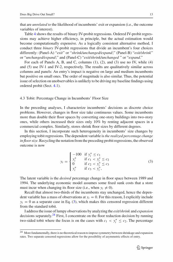
4.3 Tobit: Percentage Change in Incumbents’ Floor Size

In the preceding analyses, I characterize incumbents’ decisions as discrete choiceproblems. However, changes in floor size take continuous values. Some incumbentsmore than double their floor spaces by converting one-story buildings into two-storyones, while others increased their sizes only 10% by renting adjacent spaces in acommercial complex. Similarly, stores shrink floor sizes by different degrees.

In this section, I incorporate such heterogeneity in incumbents’ size changes byemploying tobit regressions. The dependent variable is the realized percentage changein floor size. Recycling the notation from the preceding probit regressions, the observedoutcome is now

yi =

⎧⎪⎪⎨

⎪⎪⎩

−100 if y∗i ≤ c1

y∗i if c1 < y∗

i ≤ c20 if c2 < y∗

i ≤ c3y∗

i if c3 < y∗i ,

(3)

The latent variable is the desired percentage change in floor space between 1989 and1994. The underlying economic model assumes some fixed sunk costs that a storemust incur when changing its floor size (i.e., when yi �= 0).

Recall that almost two-thirds of the incumbents stay unchanged, hence the depen-dent variable has a mass of observations at yi = 0. For this reason, I explicitly includeyi = 0 as a separate case in Eq. (3), which makes this censored regression differentfrom the standard tobit.

I address the issue of lumpy observations by analyzing the exit/shrink and expansiondecisions separately.24 First, I concentrate on the floor reduction decision by runningtwo-sided tobit where the focus is on the cases with c1 < y∗

i ≤ c2. The percentage

24 More fundamentally, there is no theoretical reason to impose symmetry between shrinkage and expansionrates. Two separate censored regressions allow for the possibility of asymmetric effects of entry.

123

14 M. Igami

Tabl

e4

Thr

eese

tsof

bina

ryIV

-pro

bitr

egre

ssio

ns

Dep

.var

.:D

ecis

ion

Not

toE

xit

(1)

(2)

(3)

(4)

(5)

A.“

Exi

t”or

“Sh

rink

/Unc

hang

ed/E

xpan

d”

Tre

ated

:lar

ge−0

.33

(.28

)−1

.36

(.58

)**

−1.4

2(.

66)*

*−2

.04

(2.6

1)−3

.74

(4.7

5)

Tre

ated

:med

ium

−0.4

9(.

31)

−0.8

3(.

32)*

*−0

.90

(.38

)**

−0.6

0(1

.22)

−0.4

2(4

.01)

Tre

ated

:sm

all

0.22

(.41

)0.

12(.

41)

0.08

(.46

)1.

20(1

.18)

1.40

(5.0

7)

Tre

ated

*flo

or3.

17e−

4(1

.65e

−4)*

3.11

e−4

(1.6

7e−4

)*3.

18e−

4(4

.45e

−4)

9.46

e−4

(7.8

4e−4

)

Floo

r7.

36e−

5(5

.24e

−5)

8.62

e−5

(5.6

4e−5

)8.

56e−

5(6

.18e

−5)

7.03

e−5

(5.3

5e−5

)

Lar

ge0.

59(.

17)*

**0.

29(.

25)

0.25

(.26

)0.

42(.

33)

0.36

(.28

)

Med

ium

0.47

(.14

)***

0.43

(.14

)***

0.45

(.15

)***

0.50

(.18

)***

0.40

(.18

)**

Con

stan

t(=

Smal

l)0.

98(.

10)*

**0.

96(.

10)*

**1.

18(.

56)*

*0.

96(.

70)

0.57

(1.9

0)

Con

trol

sN

oN

oY

esY

esY

es

Inst

rum

ents

No

No

No

IV-1

IV-2

Obs

erva

tions

912

912

912

912

912

Pseu

doR

2.0

3.0

5.0

9–

–

Dep

.var

.:D

ecis

ion

Not

toE

xito

rSh

rink

(1)

(2)

(3)

(4)

(5)

B.“

Exi

t/Sh

rink

”or

“U

ncha

nged

/Exp

and”

Tre

ated

:lar

ge−0

.13

(.35

)−0

.72

(.49

)−0

.46

(.54

)−1

.65

(1.4

2)−3

.25

(2.5

0)

Tre

ated

:med

ium

−0.5

2(.

24)*

*−0

.65

(.25

)***

−0.6

1(.

24)*

*−0

.10

(.83

)−0

.25

(1.0

8)

Tre

ated

:sm

all

0.37

(.41

)0.

33(.

41)

0.35

(.46

)0.

91(1

.03)

0.77

(1.1

0)

Tre

ated

*flo

or1.

30e−

4(.

81e−

4)0.

91e−

4(.

83e−

4)4.

45e−

4(2

.12e

−4)*

*7.

32e−

4(3

.53e

−4)*

*

Floo

r0.

53e−

5(1

.88e

−5)

1.38

e−5

(1.9

9e−5

)0.

60e−

5(2

.63e

−5)

−0.1

9e−5

(2.9

3e−5

)

Lar

ge0.

09(.

14)

0.06

(.17

)0.

05(.

18)

0.12

(.21

)0.

17(.

22)

123


Tabl

e4

cont

inue

d

Dep

.var

.:D

ecis

ion

Not

toE

xito

rSh

rink

(1)

(2)

(3)

(4)

(5)

Med

ium

−0.0

1(.

12)

−0.0

1(.

12)

0.02

(.12

)−0

.02

(.15

)−0

.03

(.14

)C

onst

ant(

=Sm

all)

0.83

(.09

)***

0.83

(.09

)***

0.55

(.49

)0.

25(.

53)

0.29

(.59

)C

ontr

ols

No

No

Yes

Yes

Yes

Inst

rum

ents

No

No

No

IV-1

IV-2

Obs

erva

tions

912

912

912

912

912

Pseu

doR

2.0

1.0

1.0

4–

–

Dep

.var

.:D

ecis

ion

Not

toE

xit,

Shri

nk,o

rSt

ayU

ncha

nged

(1)

(2)

(3)

(4)

(5)

C.“

Exi

t/Sh

rink

/Unc

hang

ed”

or“

Exp

and”

Tre

ated

:lar

ge0.

23(.

30)

−0.6

6(.

60)

−0.5

4(.

68)

−3.5

6(1

.53)

**−1

.90

(1.8

5)

Tre

ated

:med

ium

−0.7

3(.

33)*

*−0

.89

(.31

)***

−1.0

2(.

30)*

**0.

50(.

77)

0.67

(1.0

2)

Tre

ated

:sm

all

0.27

(.31

)0.

22(.

32)

0.31

(.29

)2.

22(1

.12)

**2.

11(1

.25)

*

Tre

ated

*flo

or1.

57e−

4(.

97e−

4)1.

33e−

4(1

.03e

−4)

5.72

e−4

(2.1

5e−4

)***

4.12

e−4

(2.6

2e−4

)

Floo

r1.

19e−

5(1

.90e

−5)

0.46

(2.0

0e−5

)−1

.61e

−5

(2.5

6e−5

)−0

.74e

−5

(2.8

5e−5

)

Lar

ge0.

39(.

13)*

**0.

33(.

17)*

0.39

(.18

)**

0.72

(.19

)***

0.62

(.21

)***

Med

ium

0.36

(.14

)**

0.35

(.14

)**

0.31

(.14

)**

0.23

(.17

)0.

22(.

17)

Con

stan

t(=

Smal

l)−1

.29

(.10

)***

−1.3

0(.

10)*

**−0

.74

(.44

)*−1

.12

(.58

)*−1

.24

(.61

)**

Con

trol

sN

oN

oY

esY

esY

es

Inst

rum

ents

No

No

No

IV-1

IV-2

Obs

erva

tions

912

912

912

912

912

Pseu

doR

2.0

2.0

3.0

6–

–

Stan

dard

erro

rs(c

lust

ered

by20

2to

wns

)in

pare

nthe

ses;

*si

gnif

ican

tat1

0%;*

*si

gnif

ican

tat5

%;*

**si

gnif

ican

tat1

%

123

16 M. Igami

change in floor space is left-censored at −100 (i.e., exit) and right-censored at 0, thelatter of which encompasses stores’ decisions to both “stay unchanged” and “expand.”

Second, I exclusively analyze the floor expansion decision by conducting one-sidedtobit where I focus on the cases with c3 < y∗

i . Here the percentage change in floorspace is left-censored at 0 and not right-censored.

Table 5 presents two-sided tobit estimation results on incumbents’ decisions toshrink floor space. Here again, large and medium supermarkets respond “negatively”to the new entry of large rivals by shrinking their own size, or by exiting the townaltogether. In contrast, small supermarkets are less inclined to shrink or exit.

Table 6 tells a similar story regarding the floor expansion decision of incumbents.Medium stores tend not to expand their shopping space, followed by large incumbentsto a lesser degree. Again, small supermarkets seem to respond more “aggressively”by expanding their size although coefficients are not very precisely estimated.

4.4 Discussion

The basic finding from these empirical analyses is that the entry of new large rivalsaffect incumbents differently depending on the latter’s sizes. In other words, incum-bents of different sizes face different incentives in responding to the entry shock.

This simple observation implies that large, medium, and small supermarkets offerdifferentiated services from the perspective of consumers. Hence the results high-light the role of product differentiation in relaxing competition, which is the commoninsight from numerous theoretical studies (see Sect. 2).

How do supermarkets’ retail services differ by store sizes? The most importantdifferentiation mechanism is that, while larger supermarkets offer a wider variety ofmerchandise for weekend shopping trips, consumers use their nearest (often small)supermarkets for quick, daily purchase of fresh foods (fish, vegetables, and meats).The latter is the principal mode of shopping in Tokyo.

Three demand-side factors may explain the high frequency of fresh-food shopping.First, houses (and therefore refrigerators) are small in Tokyo, leaving no storage space.Second, many Japanese are obsessed with the freshness of meat, vegetables, and espe-cially fish. Third, the female labor-force participation rate is lower in Japan than inmost developed economies, so that there are still many “professional” housewives.

The most intriguing feature of the estimation results is that small incumbents arenot just insulated from the increased competition at the top end of the size spectrum.Small supermarkets seem to benefit from the entry of new big rivals. An economicinterpretation of this finding would need to rely on some sort of positive externalitiesfrom the new entrant. Since it is not very conceivable to imagine new entrants directlyfacilitating small incumbents on the supply side, the positive externalities likely comefrom the demand side.

One example is the increased traffic of shoppers in town, attracted by new big retail-ers. Such is the theoretical model of Zhu et al. (2006), which incorporates both productdifferentiation and positive demand externality of new entry in the retail context. Myfindings fit well with their prediction that the tradeoff between the business-steal-ing effect (i.e., increased competition from new entrants) and the positive demand

123


Tabl

e5

Shri

nkag

e:tw

o-si

ded

Tobi

treg

ress

ions

ofch

ange

inflo

orsi

ze(%

)

Dep

.var

.:C

hang

ein

Flo

orSi

ze(%

)

(1)

(2)

(3)

(4)

(5)

Tre

ated

:lar

ge−3

3.13

(54.

79)

−169

.27

(111

.22)

−132

.86

(113

.45)

−61.

47(7

3.30

)−6

63.0

8(7

04.9

6)

Tre

ated

:med

ium

−96.

04(4

0.95

)**

−128

.44

(47.

86)*

*−1

19.9

5(4

9.75

)**

−12.

49(4

6.26

)−5

9.64

(266

.22)

Tre

ated

:sm

all

65.5

1(6

3.15

)55

.71

(63.

21)

56.0

1(6

4.38

)30

.33

(48.

97)

224.

67(3

06.8

1)

Tre

ated

*flo

or31

.30e

−3(2

3.49

e−3)

25.4

6e−3

(23.

21e−

3)17

.31e

−3(8

.60e

−3)*

*15

3.36

e−3

(102

.75e

−3)

Floo

r31

.75e

−4(4

6.35

e−4)

48.8

4e−4

(48.

38e−

4)4.

22e−

4(1

2.34

e−4)

29.4

4e−4

(65.

91e−

4)

Lar

ge47

.89

(25.

36)*

32.4

2(3

3.29

)28

.90

(33.

78)

2.67

(9.7

6)56

.38

(47.

31)

Med

ium

29.3

0(2

2.58

)27

.15

(22.

64)

33.2

5(2

2.55

)0.

73(5

.29)

29.2

7(2

9.39

)

Con

stan

t(=

Smal

l)14

6.36

(23.

28)*

**14

4.41

(23.

13)*

**11

1.59

(86.

08)

12.1

1(3

1.14

)53

.10

(143

.81)

Con

trol

sN

oN

oY

esY

esY

es

Inst

rum

ents

No

No

No

IV-1

IV-2

Obs

erva

tions

912

912

912

912

912

Lef

t-ce

nsor

edat

−100

%94

9494

9494

Unc

enso

red

9292

9292

92

Rig

ht-c

enso

red

at0%

726

726

726

726

726

Pseu

doR

2.0

1.0

1.0

2–

–

Stan

dard

erro

rs(c

lust

ered

by20

2to

wns

)in

pare

nthe

ses;

*si

gnif

ican

tat1

0%;*

*si

gnif

ican

tat5

%;*

**si

gnif

ican

tat1

%

123

18 M. Igami

Tabl

e6

Exp

ansi

on:o

ne-s

ided

Tobi

treg

ress

ions

ofch

ange

inflo

orsi

ze(%

)

Dep

.var

.:C

hang

ein

Flo

orSi

ze(%

)

(1)

(2)

(3)

(4)

(5)

Tre

ated

:lar

ge11

.98

(23.

37)

−42.

98(4

8.91

)−2

4.45

(50.

15)

−259

.82

(150

.37)

*−1

33.9

7(1

54.0

8)

Tre

ated

:med

ium

−66.

47(3

0.18

)**

−75.

52(3

0.93

)**

−79.

45(3

1.40

)**

66.9

0(7

6.88

)82

.17

(74.

11)

Tre

ated

:sm

all

31.7

0(2

5.68

)28

.76

(25.

77)

33.2

9(2

8.35

)18

4.73

(114

.36)

*17

5.06

(109

.14)

*

Tre

ated

*flo

or9.

13e−

3(6

.91e

−3)

5.66

e−3

(7.0

5e−3

)43

.65e

−3(2

1.15

e−3)

**31

.44e

−3(2

1.45

e−3)

Floo

r3.

89e−

4(1

8.98

e−4)

−.16

e-4

(19.

03e−

4)−1

6.22

e−

4(2

5.03

e−4)

−10.

43e−

4(2

5.21

e−4)

Lar

ge21

.92

(12.

15)*

19.9

7(1

5.45

)23

.88

(15.

42)

53.8

8(2

1.23

)**

44.6

6(2

0.48

)**

Med

ium

28.4

7(1

1.22

)**

28.2

2(1

1.29

)**

24.2

1(1

1.24

)**

15.2

0(1

6.50

)13

.69

(15.

77)

Con

stan

t(=

Smal

l)−1

11.7

5(1

1.95

)***

−111

.89

(11.

97)*

**−4

7.51

(44.

57)

−98.

83(5

5.73

)*−1

03.6

8(5

4.88

)*

Con

trol

sN

oN

oY

esY

esY

es

Inst

rum

ents

No

No

No

IV-1

IV-2

Obs

erva

tions

912

912

912

912

912

Lef

t-ce

nsor

edat

0%77

577

577

577

577

5

Unc

enso

red

137

137

137

137

137

Pseu

doR

2.0

1.0

1.0

2–

–

Stan

dard

erro

rs(c

lust

ered

by20

2to

wns

)in

pare

nthe

ses;

*si

gnif

ican

tat1

0%;*

*si

gnif

ican

tat5

%;*

**si

gnif

ican

tat1

%

123


externality (i.e., increased demand thanks to new entrants) hinges on the degree ofdifferentiation between entrants and incumbents.

Existing large and medium supermarkets suffer higher exit rates because theydirectly compete with the new big rivals at the same end of the store-size spectrum.Small supermarkets, in contrast, stand at the other end of the product space, servingdifferent demands, and are thus insulated from the business-stealing effect of the newentry. On average, the small incumbents benefit from the entrants probably becausethe latter attracts an additional flow of shoppers to the neighborhood.

Aside from the decisions to exit, incumbents’ incentives in changing store size seemquite nuanced in some size categories. First, the incentive for medium supermarketsnot to expand is understandable. They already suffer from the proximity (in size) tothe new competitor. There is no reason to spend their shrinking profits to get evencloser in size to their big rivals.

Second, the story could be more complicated for large incumbents. On the onehand, they, too, may want to follow medium stores’ strategy and distance themselvesfrom the new entrants by shrinking floor space. On the other hand, however, largeincumbents already belong to roughly the same size segment as new entrants, wheretheir central appeal to consumers is to offer the widest variety of merchandises intown.

Hence, it would not be totally surprising if some of them choose to expand floorspace, in an effort to regain their former position as the champion of one-stop shop-ping. They would race to the top end of the size spectrum to attract weekend shoppersback. I suspect that this mixture of incentives to shrink and expand might lie behindthe estimation results on large incumbents, which are generally negative but not asprecisely estimated as the response of medium stores.

Finally, why do the small supermarkets expand? Two mechanisms may possiblybe at work. One is that the increased exits among medium stores leave some nicheon the size spectrum. Even though it seems risky to become closer in size to the newbig entrants, small stores’ initial positions are so distant from the high end of theproduct space that they might be able to capture the now under-served customer seg-ment, without serious concerns over direct competition with the big entrant. The otherpossible reasoning is that the arrival of the new product (i.e., big-box retail service)somehow shifts upwards the entire product space effectively demanded by shoppers.The latter mechanism is reminiscent of Sutton’s (1991) endogenous sunk cost theory.These explanations are not mutually exclusive.

These potentially complicated incentives of floor shrinkage/expansion seem tosuggest room for further investigation—both theoretical and empirical—on productdifferentiation in conjunction with entry and exit.

5 Conclusion

Instead of driving out small rivals, large entrants seem to improve their survival pros-pects. This paper presents new evidence that supports the economic theory of prod-uct differentiation, and introduces the perspective of product differentiation to theempirical analysis of entry and exit.

123

20 M. Igami

I conduct ordered and IV probit regressions of each incumbent store’s responses(i.e., exit, stay and shrink, stay unchanged, or stay and expand). The results suggestthat, even after accounting for both the (ordered) discrete nature of the decision prob-lem and the potential issue of new entrants’ town selection based on the unobservabletown characteristics, the main findings stand out: Large and medium incumbents areadversely affected by the new entries of big rivals, whereas small incumbents seem tobenefit from them. The results from tobit regressions on the percentage change of floorspace further confirms this contrast between large, medium, and small supermarkets.

These findings imply that store size functions as a key dimension of product differ-entiation among retailers.25 On the one hand, large and medium incumbents competeas closer substitutes to new large entrants. On the other hand, small supermarkets—thanks to a sufficient degree of differentiation—benefit from the increased traffic ofshoppers that is generated by the entrants.

Consequently, this research critically examines the conventional notion that bigdrives out small, a notion that continues to motivate size-based entry regulations inmany economies, both developed and emerging. Ironically, such policies appear toshield big retailers from competition and even preclude small stores from enjoying theincreased customer flow that can be generated by large new entrants. The specifics ofgeographical and regulatory setting may differ by country and region, but these basiceconomic forces of product differentiation and entry/exit are likely to be at play inmany markets.

Acknowledgments I thank Jinyong Hahn, Hidehiko Ichimura, Toshiaki Iizuka, Edward Leamer,Rosa Matzkin, Hiroshi Ohashi, Connan Snider, Raphael Thomadsen, and seminar participants at the Univer-sity of Tokyo, the 2007 Japanese Economic Association Annual Spring Meeting at Osaka Gakuin University,and UCLA, for invaluable suggestions. I am grateful to the editor, Lawrence White, and the two anony-mous referees, for thoughtful comments. I thank Evan Gill, Matthew Khalil Hill, and Maki Komatsu foreditorial assistance, Saneaki Obata for industry expertise, and my local supermarkets CSN (small) and LifeExtra (medium) for inspiration. Financial support from the Ito Foundation and the Nozawa Fellowship aregratefully acknowledged.

Open Access This article is distributed under the terms of the Creative Commons Attribution Noncom-mercial License which permits any noncommercial use, distribution, and reproduction in any medium,provided the original author(s) and source are credited.

References

Anderson, S. P., de Palma, A., & Thisse, J.-F. (1992). Discrete choice theory of product differentia-tion. Cambridge, MA: MIT Press.

Arai, Y. (1996). Seikatsu-ken no keikaku. In Y. Arai, K. Okamoto, H. Kamiya, & T. Kawaguchi (Eds.), Toshino kuukan to jikan: Seikatsu-katsudou no jikan-chirigaku (pp. 73–80). Tokyo: Kokonshoin.

Basker, E. (2005). Job creation or destruction? Labor-market effects of Wal-Mart expansion. Review ofEconomics and Statisitics, 87(1), 174–183.

Basker, E. (2007). The causes and consequences of Wal-Mart’s growth. Journal of Economic Perspec-tives, 21(3), 177–198.

25 Hence it is not surprising that the retail chains known for “hypermart” formats, such as Tesco andCarrefour, are introducing new store formats that are much smaller than their original sizes (Tesco Expressand Carrefour Express). Even Wal-Mart, the synonym of big-box retailer, developed smaller store formatsin Mexico and is now considering their transplantation to rural China (Financial Times, December 2, 2010).

123


Borenstein, S., & Netz, J. (1999). Why do all the flights leave at 8am?: Competition and departure-timedifferentiation in airline markets. International Journal of Industrial Organization, 17, 611–640.

D’Aspremont, C., Gabszewicz, J. J., & Thisse, J.-F. (1979). On Hotelling’s ‘stability in competition’.Econometrica, 47, 1145–1150.

Ellickson, P. B. (2007). Does Sutton apply to supermarkets?. RAND Journal of Economics, 38(1), 43–59.Ellickson, P. B., & Misra, S. (2008). Supermarket pricing strategies. Marketing Science, 27(5), 811–828.Hausman, J. A., & Leibtag, E. (2007). Consumer benefits from increased competition in shopping

outlets: Measuring the effect of Wal-Mart. Journal of Applied Econometrics, 22(7), 1157–1177.Irmen, A., & Thisse, J.-F. (1998). Competition in multi-characteristics spaces: Hotelling was almost

right. Journal of Economic Theory, 78, 76–102.Japan Fair Trade Commission. (2005). Marubeni Kabushikigaisha niyoru Kabushikigaisha Daiei tou heno

shusshi nitsuite. Retrieved September 23, 2009, from http://www.jftc.go.jp/ma/jirei2/H17jirei12-02.html.

Kawaguchi, T. (1996). Seikatsu no jikuukan to shogyo katsudou. In Y. Arai, K. Okamoto, H. Kami-ya, & T. Kawaguchi (Eds.), Toshi no kuukan to jikan: Seikatsu-katsudou no jikan-chirigaku (pp. 157–176). Tokyo: Kokonshoin.

Lewis, W. W. (2004). The power of productivity: Wealth, poverty, and the threat to global stability. Chicago,IL: The University of Chicago Press.

Masuda, E. (2002). Tokyo-ken Korekara Nobiru Machi [Towns with High Growth Potential in GreaterTokyo]. Tokyo: Kodansha.

Mazzeo, M. J. (2002). Product choice and oligopoly market structure. RAND Journal of Econom-ics, 33(2), 221–242.

Minakata, T. (2004). Nihon no Kouri-gyo to Ryutsu-seisaku. Tokyo: Chuo-Keizai-Sha.Neven, D., & Thisse, J.-F. (1990). On quality and variety competition. In J. J. Gabszewicz, J.-F. Richard, &

L. Wolsey (Eds.), Economic decision-making: Games, econometrics and optimisation (pp.175–199). Amsterdam: North Holland.

Perloff, J. M., & Salop, S. C. (1985). Equilibrium with product differentiation. The Review of EconomicStudies, 52(1), 107–120.

Shaked, A., & Sutton, J. (1982). Relaxing price competition through product differentiation. Review ofEconomic Studies, 49, 3–13.

Shogyokai. (1990 & 1995). Japan Supermarket Directory [Nihon Supermarket Meikan]. Tokyo: Shogyokai.Smith, H. (2004). Supermarket choice and supermarket competition in market equilibrium. Review of

Economic Studies, 71, 235–263.Sobel, R. S., & Dean, A. M. (2008). Has Wal-Mart Buried Mom and Pop? The impact of Wal-Mart on

self-employment and small establishments in the United States. Economic Inquiry 46(4), 676–695.Sutton, J. (1991). Sunk costs and market structure: Price competition, advertising, and the evolution

of concentration. Cambridge, MA: MIT Press.Toyokeizai. (1995). Metropolitan commercial map 1995 [Shutoken Shogyochi Map 1995]. Tokyo:

Toyokeizai.Wal-Mart Watch. (2005). Annual Report 2005: Low Price at What Cost? Retrieved from http://

walmartwatch.com/img/sitestream/pdf/2005-annual-report.pdf.Zhu, T., Singh, V. & Dukes, A. (2006). Local competition and impact of entry by a discount retailer.

Working Paper, University of Toronto.

123

http://www.jftc.go.jp/ma/jirei2/H17jirei12-02.html

http://www.jftc.go.jp/ma/jirei2/H17jirei12-02.html

http://walmartwatch.com/img/sitestream/pdf/2005-annual-report.pdf

http://walmartwatch.com/img/sitestream/pdf/2005-annual-report.pdf

entry, exit, and differentiation in the supermarket industry · 2017-08-28 · jel classiﬁcation...

Documents