Equilibrium Strategies for Multiple Interdictors on a CommonNetwork

Harikrishnan Sreekumaran∗ Ashish R. Hota† Andrew L. Liu‡ Nelson A. Uhan§

Shreyas Sundaram¶

June 26, 2017

Abstract

In this work, we introduce multi-interdictor games, which model interactions among multiple in-terdictors with differing objectives operating on a common network. As a starting point, we focus onshortest path multi-interdictor (SPMI) games, where multiple interdictors try to increase the shortestpath lengths of their own adversaries attempting to traverse a common network. We first establish resultsregarding the existence of equilibria for SPMI games under both discrete and continuous interdictionstrategies. To compute such an equilibrium, we present a reformulation of the SPMI game, which leadsto a generalized Nash equilibrium problem (GNEP) with non-shared constraints. While such a problemis computationally challenging in general, we show that under continuous interdiction actions, a SPMIgame can be formulated as a linear complementarity problem and solved by Lemke’s algorithm. In ad-dition, we present decentralized heuristic algorithms based on best response dynamics for games underboth continuous and discrete interdiction strategies. Finally, we establish theoretical lower bounds onthe worst-case efficiency loss of equilibria in SPMI games, with such loss caused by the lack of coordi-nation among noncooperative interdictors, and use the decentralized algorithms to numerically study theaverage-case efficiency loss.

1 Introduction

In an interdiction problem, an agent attempts to limit the actions of an adversary operating on a networkby intentionally disrupting certain components of the network. Such problems are usually modeled in theframework of leader-follower games and can be formulated as bilevel optimization problems. Interdictionmodels have been used in various military and homeland security applications, such as dismantling drugtraffic networks [51], preventing nuclear smuggling [34] and planning tactical air strikes [24]. Interdictionmodels have also found applications in other areas such as controlling the spread of pandemics [4] anddefending attacks on computer communication networks [44].

Traditionally, interdiction problems have been analyzed from a centralized perspective; namely, a singleagent is assumed to analyze, compute and implement interdiction strategies. In many situations, however, itmight be desirable and even necessary to consider an interdiction problem from a decentralized perspective.Arguably the most prominent example of such situations today is the war against the terrorist group, the∗American Airlines, Fort Worth, Texas USA. Email: harikrishnan.sreekumaran@gmail.com†School of Electrical and Computer Engineering, Purdue University, West Lafayette, Indiana, USA. Email: ahota@purdue.edu‡Corresponding author. School of Industrial Engineering, Purdue University, West Lafayette, Indiana, USA. Email: an-

drewliu@purdue.edu§Mathematics Department, United States Naval Academy, Annapolis, Maryland, USA. Email: uhan@usna.edu¶School of Electrical and Computer Engineering, Purdue University, West Lafayette, Indiana, USA. Email: sun-

dara2@purdue.edu

1

Islamic State of Iraq and Syria (ISIS, also known as ISIL or Daesh). It is believed that oil smuggling is the“biggest single source of revenue” of ISIS [45], and hence, a sensible strategy to defeat ISIS is to disrupt theiroil smuggling. Such a strategy indeed has been deployed by the multiple parties involved in the war [1, 42].The parties involved, however, which include the US-led coalition, Russia, Turkey, Iran, among others,do not operate as a single coalition, and often do not share information [26]. Without any coordinationbetween the parties, one might expect that a decentralized interdiction strategy may be inefficient comparedto one determined by a central decision maker. A central decision maker in the war against ISIS is ofcourse impractical, and hence, we would like to understand better the equilibrium state of such settings withmultiple interdictors on a common network, and especially the efficiency loss due to the lack of cooperationamong the interdictors. This is both the motivation and the focus of this paper.

In this paper, we introduce decentralized multiple interdictor games, in which multiple agents withdiffering objectives are interested in interdicting parts of a common network. We focus on a specific class ofthese games, which we call shortest path multi-interdictor (SPMI) games. We investigate various propertiesof equilibria in SPMI games, including their existence and uniqueness, and propose algorithms to computeequilibria of these games. Using these algorithms, we also conduct numerical studies on the efficiency lossof equilibria in the SPMI game compared to optimal solutions obtained through centralized decision making.

Decentralized network interdiction games, as will be formally defined in Section 2, appear to be new.To the best of our knowledge, there has been no previous research on such games. As a result, not muchis known about the inefficiency of equilibria for these games or intervention strategies to reduce such in-efficiencies. There has been a considerable amount of work, however, on interdiction problems from acentralized decision-maker’s perspective. As mentioned earlier, interdiction problems have been studied inthe context of various military and security applications. For extensive reviews of the existing academicliterature on interdiction problems, we refer the readers to Church et al. [9] and Smith and Lim [44].

There have also been many studies on the inefficiency of equilibria in other game-theoretic settings.Most of the efforts have been focused on routing games [37,50], in which selfish agents route traffic througha congested network, and congestion games [40], a generalization of routing games. Some examples include[5,8,10,12,41,46]. Several researchers have also studied the inefficiency of equilibria in network formationgames, in which agents form a network subject to potentially conflicting connectivity goals [2, 3, 17]. Theinefficiency of equilibria has been studied in other games as well, such as facility location games [49],scheduling games [31], and resource allocation games [28, 29]. Almost all of the work described abovestudy the worst-case inefficiency of a given equilibrium concept. Although a few researchers have studiedthe average inefficiency of equilibria, either theoretically or empirically, and have used it as a basis to designinterventions to reduce the inefficiency of equilibria [11,47], research in this direction has not received muchattention.

One potential reason for the lack of attention paid to multiple interdictor games may be that such gamesoften involve nondifferentiability, as each interdictor’s optimization problem usually entails a max-min typeof objective function. Games involving nondifferentiable functions are generally challenging, in terms ofboth theoretical analysis of their equilibria and computing an equilibrium. While in some cases (such asin the case of shortest path interdiction), a smooth formulation (through total unimodularity and duality) ispossible, such a reformulation will yield a generalized Nash equilibrium problem (GNEP), in which both theagents’ objective functions as well as their feasible action spaces depend on other agents’ actions. Althoughthe conceptual framework of GNEPs can be dated to Debreu [14], rigorous theoretical and algorithmictreatments of GNEPs began much later (see [19], for example, for a literature review). Several techniqueshave been proposed to solve GNEPs, including penalty-based approaches [20, 23], variational-inequality-based approaches [36], Newton’s method [15], projection methods [52], and relaxation approaches [32,48].Most of the work on GNEPs has focused on games with shared constraints due to their tractability [18, 25].In such games, a set of identical constraints appear in each agent’s feasible action set. However, as will beseen later, in a typical decentralized network interdiction game, the constraints involving multiple agents’

2

actions that appear in each agent’s action space are not identical. As a result, such games give rise to morechallenging instances of GNEPs.

Based on the discussions above, the major contributions of this work are as follows.

• First, we establish the existence of pure-strategy equilibria for SPMI games with continuous inter-diction. In SPMI games with discrete interdiction, the existence of a pure strategy Nash equilibrium(PNE) is more subtle. We first demonstrate that a PNE does not necessarily exist in SPMI games withdiscrete interdiction. However, when all agents have the same source-target pairs (i.e., multiple agentstry to achieve a common goal independently), a PNE exists in these games.

• Second, for SPMI games under continuous interdiction, we show that each agent’s optimization prob-lem can be reformulated as a linear programming problem. As a result, the equilibrium conditions ofthe game can be reformulated as a linear complementarity problem with some favorable properties,allowing it to be solved by the well-known Lemke algorithm [33]. For SPMI games with discrete inter-diction (and continuous interdiction), we present decentralized algorithms for finding an equilibrium,based on the well-known best-response dynamics (or Gauss-Seidel iterative) approach. While suchan approach is only a heuristic method in general, convergence can be established for the special casewhen the agents have common source-target pairs. For more general cases, we obtain encouragingnumerical results for the performance of the method on several classes of network structures.

• Third, we measure the efficiency loss in SPMI games due to the lack of coordination among noncoop-erative interdictors, compared to a centralized interdiction strategy (that is, a strategy implemented bya single interdictor with respect to all the adversaries). In particular, we establish a theoretical lowerbound for the worst-case price of anarchy of SPMI games under continuous interdiction. Such an ef-ficiency loss measure, however, may be too conservative, and so we use the decentralized algorithmsto numerically quantify the average-case efficiency loss over some instances of SPMI games. Theseresults can help central authorities design mechanisms to reduce such efficiency losses for practicalinstances.

The remainder of this paper is organized as follows. We begin in Section 2 with definitions and formu-lations of general multi-interdictor games and the specific SPMI games. In Section 3, we present the maintheoretical results of the paper, including an analysis of the existence and uniqueness of equilibria in SPMIgames. In Section 4 we investigate algorithms for solving SPMI games. We describe a centralized algorithmbased on a linear complementarity formulation, as well as decentralized algorithms for computing equilibriaof SPMI games. We also present the results of our computational experiments with these algorithms forcomputing equilibria as well as quantifying the price of anarchy for various instances. Finally, in Section 5,we provide some concluding remarks.

2 Games with Multiple Interdictors on a Common Network

2.1 General Formulation

Network interdiction problems involve interactions between two types of parties – adversaries and interdic-tors – with conflicting interests. An adversary operates on a network and attempts to optimize some objec-tive, such as the flow between two nodes. An interdictor tries to limit an adversary’s objective by changingelements of the network, such as the arc capacities. Such interactions have historically been viewed from aleader-follower-game perspective. The interdictor acts as the leader and chooses an action while anticipatingthe adversary’s potential responses, while the adversary acts as the follower and makes a move after observ-ing the interdictor’s actions. From the interdictor’s perspective, this captures the pessimistic viewpoint ofguarding against the worst possible result given its actions.

3

In this work, we consider strategic interactions among multiple interdictors who operate on a commonnetwork. The interdictors may each have their own adversary or they may have a common adversary. Ifthere are multiple adversaries, we assume there is no strategic interaction among them. We also assume thatthe interdictors are allies in the sense that they are not interested in deliberately impeding each other.

Formally, we have a setF = 1, . . . , F of interdictors or agents, who operate on a networkG = (V,A),where V is the set of nodes and A is the set of arcs. Each agent’s actions or decisions correspond tointerdicting each arc of the network with varying intensity: the decision variables of agent f ∈ F aredenoted by xf ∈ Xf ⊂ R|A|, where Xf is an abstract set that constrains agent f ’s decisions. For anyagent f ∈ F , let x−f denote the collection of all the other agents’ decision variables; that is, x−f =(x1, . . . , xf−1, xf+1, . . . , xF ). The network obtained after every agent executes its decisions or interdictionstrategies is called the aftermath network. The strategic interaction between the agents occurs due to thefact that the properties of each arc in the aftermath network are affected by the combined decisions of all theagents.

In addition to the abstract constraint set Xf , we assume that each agent f ∈ F has a total interdictionbudget of bf . The cost of interdicting an arc is linear in the intensity of interdiction; in particular, agent f ’scost of interdicting arc (u, v) by xfuv units is cfuvx

fuv. Without loss of generality, we assume that bf > 0 and

cfuv > 0 for each arc (u, v) ∈ A and for each agent f ∈ F . The optimization problem for each agent f ∈ Fis:

maximizexf

θf (xf , x−f )

subject to∑

(u,v)∈A

cfuvxfuv ≤ bf ,

xf ∈ Xf ,

(1)

where the objective function θf is agent f ’s obstruction function, or measure of how much agent f ’s adver-sary has been obstructed. Henceforth, we refer to the game in which each agent f ∈ F solves the aboveoptimization problem (1) as a decentralized multi-interdictor game. As a starting point, we restrict our at-tention to simultaneous-move games with complete information. Simultaneous-move means that the agentsmust make their decisions without being aware of the other agents’ decisions. A complete information gamemeans that the number of agents, their payoffs and their feasible action spaces are common knowledge toall the agents.

The obstruction function θf can capture various types of interdiction problems. Typically θf is the (im-plicit) optimal value function of the adversary’s network optimization problem parametrized by the agents’decisions. For example, θf might be the minimum flow cost or path length subject to flow conservation, arccapacity and side constraints in the aftermath network.

Suppose that a central planner, with a comprehensive view of the network and the agents’ objectives,could pool the agents’ interdiction resources and determine an interdiction strategy that maximizes someglobal measure of how much the agents’ adversaries have been obstructed. Let θc(x1, . . . , xF ) representthe global obstruction function for a given interdiction strategy (x1, . . . , xF ). The central planner’s problemcorresponding to the multi-interdictor game (1) is then:

maximizex1, ..., xF

θc(x1, . . . , xF )

subject to∑f∈F

∑(u,v)∈A

cfuvxfuv ≤

∑f∈F

bf ,

xf ∈ Xf ∀f ∈ F .

(2)

Without loss of generality, we assume that θc(·) ≥ 0 for any feasible (x1, . . . , xF ). We refer to (2) as the

4

centralized problem, and focus primarily on when the global obstruction function is utilitarian; that is,

θc(x1, . . . , xF ) :=∑f∈F

θf (xf , x−f ).

Note also that we assume the resources involved in the budgetary constraints may be “pooled” amongstthe interdictors. Such resources may then be allocated optimally by the central planner. The case wherethe resources are not shareable can easily be modeled by enforcing each interdictor’s resource constraintsseparately in the central planner’s problem.

As mentioned earlier, one of the goals of this work is to quantify the inefficiency of an equilibrium ofa decentralized multi-interdictor game – a decentralized solution to problem (1) – relative to a centrallyplanned optimal solution – an optimal solution to problem (2). A commonly used measure of such inef-ficiency is the price of anarchy. Formally speaking, let NI be the set of all equilibria corresponding to aspecific instance I . (In the context of multi-interdictor games, an instance consists of the network, obstruc-tion functions, interdiction budgets, and costs.) For the same instance I , let (x1∗ , . . . , xF

∗) denote a globally

optimal solution to the centralized problem (2). Then the price of anarchy of the instance I is defined as

p(I) := max(x1

N ,...,xFN )∈NI

θc(x1∗ , . . . xF∗)

θc(x1N , . . . , x

FN ). (3)

Let I be the set of all instances of a game. We assume implicitly that for all I ∈ I, the set NI is nonemptyand a globally optimal solution to the centralized problem exists. By convention, p is set to 1 if the worstequilibrium as well as the globally optimal solution to the centralized problem both have zero objectivevalue. If the worst equilibrium has a zero objective value while the globally optimal value of the centralizedproblem is positive, p is set to be infinity. In addition to the price of anarchy for an instance of a game, wealso define the worst-case price of anarchy over all instances of the game (denoted as w.p.o.a) as follows:

w.p.o.a := supI∈I

p(I). (4)

We wish to study the efficiency loss of the class of multi-interdictor games. The worst-case price of anarchyprovides a way to measure this. However, there are two major difficulties associated with this as an efficiencymeasure. First, it is well-known that the worst-case price of anarchy can be a very conservative measureof efficiency loss, since the worst case may only happen with pathological instances. Second, explicittheoretical bounds on the worst-case price of anarchy may be difficult to obtain for general classes of games.In fact most of the related research has focused on identifying classes of games for which such bounds maybe derived. In this work, we show how our proposed decentralized algorithms can be used to numericallystudy the average-case efficiency loss (denoted by a.e.l). Let I ′ ⊂ I denote a finite subset of instances, andlet |I ′| denote the cardinality of the the set I ′. Then

a.e.l(I ′) :=1

|I ′|∑I∈I′

p(I). (5)

In other words, the average-case efficiency loss is the average value of p(I) as defined in (3) over a set ofsampled instances I ′ ⊂ I of a game.

As mentioned above, the generic form of problem (1) can be used to describe various network interdic-tion settings. To start with models that are both theoretically and computationally tractable, we focus onshortest-path multi-interdictor games, which we describe in detail next.

2.2 Shortest Path Multi-interdictor Games

As the name suggests, shortest path multi-interdictor (SPMI) games involve agents or interdictors whoseadversaries are interested in the shortest path between source-target node pairs on a network. Interdictors

5

act in advance to increase the length of the shortest path of their respective adversaries by interdicting (inparticular, lengthening) arcs on the network.

To describe these games formally, we build upon the setup of the general multi-interdictor game de-scribed in Section 2.1. Each agent f ∈ F has a target node tf ∈ V that it wishes to protect from anadversary at source node sf ∈ V by maximizing the length of the shortest path between the two nodes. Theagents achieve this goal by committing some resources (e.g. monetary spending) to increase the individualarc lengths on the network: the decision variable xfuv represents the contribution of agent f ∈ F towardslengthening arc (u, v) ∈ A. The arc length duv(xf , x−f ) of arc (u, v) ∈ A in the aftermath network dependson the decisions of all the agents.

We consider two types of interdiction. The first type of interdiction is continuous: in particular,

Xf := xf ∈ R|A| : xfuv ≥ 0 ∀(u, v) ∈ A.

The arc lengths after an interdiction strategy (x1, . . . , xF ) has been executed are

duv(x1, . . . , xF ) = d0

uv +∑f∈F

xfuv ∀(u, v) ∈ A, (6)

where xfuv captures how much agent f extends the length of arc (u, v). We assume that d0uv ≥ 0 for all

(u, v) ∈ A. The second type of interdiction is discrete: in this case,

Xf := xf ∈ R|A| : xfuv ∈ 0, 1 ∀(u, v) ∈ A

and the arc lengths in the aftermath network are

duv(x1, . . . , xF ) = d0

uv + euv maxf∈F

xfuv ∀(u, v) ∈ A, (7)

where euv ∈ R≥0 is the fixed extension of arc (u, v). In other words, the length of an arc is extended by afixed amount if at least one agent decides to interdict it.

Let P f = pf1 , pf2 , . . . , p

fkf be the set of sf -tf paths available to agent f ∈ F . The length of a path

p ∈ P f is given bydp(x

1, . . . , xF ) =∑

(u,v)∈p

duv(x1, . . . , xF ), (8)

where duv(x1, . . . , xF ) is as defined in equation (6) for continuous interdiction, and as defined in (7) for thediscrete case. The optimization problem for each interdicting agent f ∈ F is then:

maximizexf

θf (xf , x−f ) ≡ minp∈Pf

dp(xf , x−f )

subject to∑

(u,v)∈A

cfuvxfuv ≤ bf ,

xf ∈ Xf .

(9)

Under continuous interdiction and assuming that Xf is nonempty, convex and compact, the feasiblestrategy set for agent f , given by xf ∈ Xf |

∑(u,v)∈A c

fuvx

fuv ≤ bf is also convex and compact. To rule

out uninteresting cases, we also assume that the feasible set for each agent is also nonempty (meaning thateach agent has the budget to interdict some arcs). Moreover, given an x−f , the objective function in (9)is the minimum of a set of affine functions of xf , and therefore continuous in xf . Thus, by Weierstrass’sextreme value theorem, each agent has an optimal strategy given the strategies of the other agents. Note,however, that the objective function in (9) is not differentiable with respect to xf in general.

For SPMI games with discrete interdiction, the feasible strategy set for each agent is finite. Thereforean optimal solution to each agent’s problem always exists with a given x−f . In the following section,we analyze the existence and uniqueness of pure strategy Nash Equilibria for SPMI games, under bothcontinuous and discrete settings.

6

3 Game Structure and Analysis

3.1 Existence of Equilibria

We first consider the existence of a Nash equilibrium of a SPMI game when interdiction decisions arecontinuous. The key is to show that the objective function in (9) θf (xf , x−f ) is concave in xf , despite thefact that it is not differentiable.

Proposition 1. Assume that the abstract set Xf in (9) is nonempty, convex and compact for each f ∈ F .The SPMI game under continuous interdiction – each agent f ∈ F solves the problem (9) with dp(xf , x−f )defined as in (8) and (6) – has a pure strategy Nash equilibrium.

Proof. Based on the assumption, the feasible region in (9) is nonempty, convex and compact. With a fixedx−f , the objective function of agent f is the minimum of a finite set of affine functions in xf , and therefore,is concave with respect to xf (Cf. [7]). Consequently, the SPMI game belongs to the class of “concavegames,” introduced in Rosen [39], and it is shown in [39] that a pure-strategy Nash equilibrium alwaysexists for a concave game.

Under discrete interdiction, the existence of a PNE is not always guaranteed when different interdictorsare competing against different adversaries. We illustrate the nonexistence of PNE in Example 1 below.

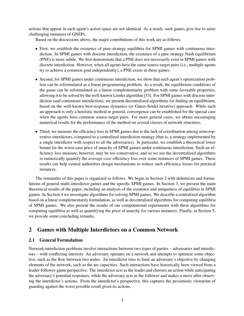
Example 1. Consider the network given in Figure 1.

s1

s2

t1, t2

b

e

c d

a

f

Figure 1: Network topology for the SPMI game in Example 1.

In this game, there are two agents – agent 1 and agent 2 – who are attempting to maximize the lengthsof the s1-t1 paths and s2-t2 paths respectively. Note that t1 = t2. The data for the problem, including initialarc lengths, cost of interdiction and arc extensions are given below in Table 1.

Arc tag Initial length Arc extension Cost to player 1 Cost to player 2

a 7 0.5 3 20b 0 2 6 20c 0 1.5 5 20d 0 6 15 15e 0 1 20 20f 1 6 15 15

Table 1: Network data for Example 1

Suppose that the budgets are b1 = 8 and b2 = 15. As a result, player 1 can either interdict the arcs a, band c one at a time, or the arcs a and c simultaneously. Similarly, player 2 can either interdict arc d or arc f .

7

Thus, player 1 has four feasible pure strategies and player 2 has two feasible pure strategies. The strategytuples along with the corresponding payoffs for each player are summarized in Table 2. It is easy to verifythat for any joint strategy profile, there is a player who would prefer to deviate unilaterally. Therefore, thisinstance of the SPMI game does not possess a PNE.

Player 1 / Player 2 d f

a 6, 1 0, 0

c 7, 1 1.5, 1.5

(a, c) 7.5, 1 1.5, 1.5

b 7, 1 2, 0

Table 2: Payoff combinations for Example 1

In the previous example, the agents have a common target node, but different source nodes. However,in the class of games in which the interdictors have a common adversary, i.e., when each agent maximizesthe shortest path between a common source-target pair, we can show that SPMI games under discrete inter-diction possess a PNE.

Consider the SPMI game where each agent is trying to maximize the shortest path lengths betweennodes s and t. Since the objective function of each agent is the same, we can write the following centralizedoptimization problem to maximize the shortest s-t path distance subject to the individual agents’ budgetconstraints. Let P st be the set of s-t paths in the network. The centralized optimization problem is:

maximizex

minp∈P st

dp(x1, x2, . . . , xF )

subject to∑

(u,v)∈A

cfuvxfuv ≤ bf ∀f ∈ F ,

xfuv ∈ 0, 1 ∀(u, v) ∈ A, f ∈ F .

(10)

The feasible solution space of the above problem is finite under individual agents’ budget constraints. There-fore, the centralized problem always has a maximum. Furthermore, the optimal solution to this problem is aPNE of the SPMI game as we show in the following result.

Proposition 2. Suppose the source and target for each agent in a SPMI game under discrete interdiction,are the same. Let x∗ denote the optimal solution of the centralized problem (10). Then x∗ is a PNE to theSPMI game.

Proof. Assume the contrary, and suppose that there is an agent h for whom there exists a unilateral deviationxf that strictly increases the path distance from source to target. By assumption, xh is feasible for thebudgetary constraints for agent h. Therefore, x ≡ (xh, x∗−h) is feasible for (10) with a strictly largerobjective value. Clearly this is a contradiction to the optimality of x∗ for (10).

3.2 Non-Uniqueness of Equilibria

Establishing sufficient conditions for a SPMI game to have a unique equilibrium is quite difficult. However,it is easy to find simple instances of SPMI games for which multiple equilibria exist. We give two suchexamples below.

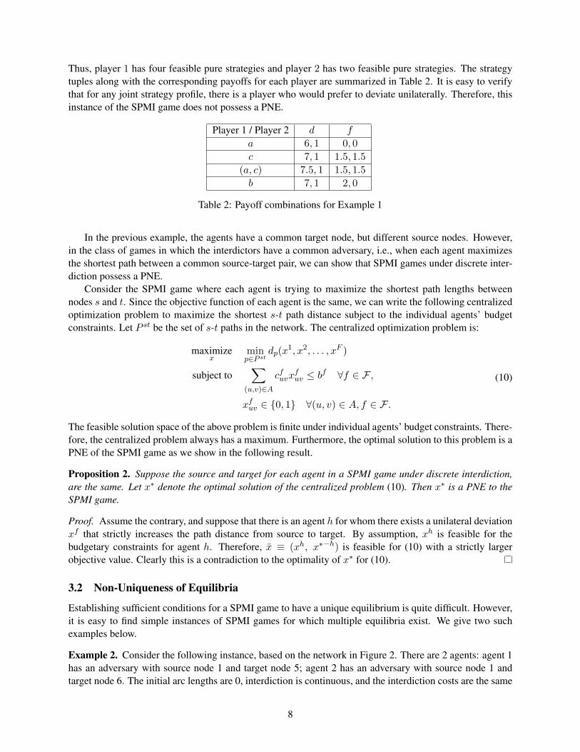
Example 2. Consider the following instance, based on the network in Figure 2. There are 2 agents: agent 1has an adversary with source node 1 and target node 5; agent 2 has an adversary with source node 1 andtarget node 6. The initial arc lengths are 0, interdiction is continuous, and the interdiction costs are the same

8

1 2 3

4 5 6

1 + ǫ 1 + ǫ

1 + ǫ 1 + ǫ

1 1 1

Figure 2: Network topology for SPMI game in Example 2.

for both agents and are given in the arc labels in Figure 2. Both agents have a budget of 1. Consider the casewhen ε = 2. In this case, it is straightforward to see that the source-target path lengths for each agent mustbe equal at an equilibrium: if the path lengths are unequal, an agent could improve its objective function byequalizing the path lengths. Therefore, in this example, any combination of decision variables that results ina shortest path length of 2/3 for each agent is a Nash equilibrium, and there is a continuum of such decisionvariable combinations. Indeed, some of such equilibria are given in Table 3 in Section 5.

Example 3. Under discrete interdiction on the same underlying network, an interesting situation occurswhen ε = 0, both agents have a budget of 1, and the arc extensions are all set to 1. In this case, anequilibrium occurs when the arcs (1, 4) and (1, 2) are interdicted by one agent each. However, there existequilibria that have inferior objective values for both agents. Indeed, the extreme case of neither agentinterdicting any arc can easily seen to be an equilibrium. This point in fact is a social utility minimizer overthe set of feasible action combinations for the two agents.

4 Computing a Nash Equilibrium

In this section we discuss algorithms to compute equilibria of SPMI games. While the general formula-tion with each agent solving (9) is sufficient for showing existence of equilibria, such a formulation is notamenable for computing an equilibrium mainly due to the ‘min’ function in the objective function. In thissection, using a well-known reformulation of shortest path problems (through total unimodularity and linearprogramming duality), we formulate the SPMI game as a generalized Nash equilibrium problem. For con-tinuous SPMI games, we further show that such a GNEP can be written as a linear complementarity problem(LCP) through the Karush-Kuhn-Tucker (KKT) optimality conditions. We then show that the resulting LCPhas favorable properties, allowing the use of Lemke’s pivoting algorithm with guaranteed convergence to asolution (as opposed to a secondary ray).

We refer to the LCP approach as a centralized approach, in the sense that the game is purely viewedas a system of equilibrium conditions, and a general algorithm capable of solving the resulting system isapplied. We also present decentralized algorithms based on best-response dynamics, which are applicable toboth continuous and discrete SPMI games. While not necessarily more computationally efficient, decentral-ized algorithms indeed have several advantages over centralized algorithms. First, a centralized approachusually relies on the first-order optimality conditions of each agent’s optimization problem. Such conditionsare not available in discrete games, where agents’ problems contain discrete variables. A decentralized ap-proach can nevertheless be applied to discrete games, as each agent’s problem can be solved by an integerprogramming algorithm, without relying on explicit optimality conditions. Second, a decentralized algo-rithm may provide insight on how a particular equilibrium is achieved among agents’ strategic interactions.Such insight is particularly useful when multiple equilibria exist, as is the case for many GNEPs. It is known

9

(for example, [35]) that a game may possess unintuitive Nash equilibria that would never be a realistic out-come. Third, a decentralized algorithm can naturally lead to multithreaded implementations that can takeadvantage of a high performance computing environment. In addition, different threads in a multithreadedimplementation may be able to find different equilibria of a game, making such an algorithm particularlysuitable for computationally quantifying the average efficiency loss of noncooperative strategies.

In the following discussion, we first present the GNEP formulation of SPMI games under continuousinterdiction. We then reformulate the GNEP as an LCP and analyze the properties of the LCP formula-tion. Finally we present the decentralized algorithms for SPMI games under both discrete and continuousinterdiction formulated as GNEPs.

4.1 Dual GNEP formulation

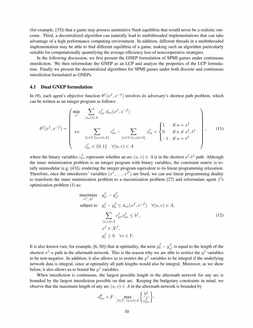
In (9), each agent’s objective function θf (xf , x−f ) involves its adversary’s shortest path problem, whichcan be written as an integer program as follows:

θf (xf , x−f ) =

minzf

∑(u,v)∈A

zfuv duv(xf , x−f )

s.t.∑

v∈V |(u,v)∈A

zfuv −∑

v∈V |(v,u)∈A

zfvu =

1 if u = sf

0 if u 6= sf , tf

−1 if u = tf

zfuv ∈ 0, 1 ∀(u, v) ∈ A

, (11)

where the binary variables zfuv represents whether an arc (u, v) ∈ A is in the shortest sf -tf path. Althoughthe inner minimization problem is an integer program with binary variables, the constraint matrix is to-tally unimodular (e.g. [43]), rendering the integer program equivalent to its linear programming relaxation.Therefore, once the interdictors’ variables (x1, . . . , xF ) are fixed, we can use linear programming dualityto transform the inner minimization problem to a maximization problem [27] and reformulate agent f ’soptimization problem (1) as:

maximizexf , yf

yftf− yf

sf

subject to yfv − yfu ≤ duv(xf , x−f ) ∀(u, v) ∈ A,∑(u,v)∈A

cfuvxfuv ≤ bf ,

xf ∈ Xf ,

yfv ≥ 0 ∀v ∈ V.

(12)

It is also known (see, for example, [6, 30]) that at optimality, the term yfu − yfsf is equal to the length of theshortest sf -u path in the aftermath network. This is the reason why we are able to restrict the yf variablesto be non-negative. In addition, it also allows us to restrict the yf variables to be integral if the underlyingnetwork data is integral, since at optimality all path lengths would also be integral. Moreover, as we showbelow, it also allows us to bound the yf variables.

When interdiction is continuous, the largest possible length in the aftermath network for any arc isbounded by the largest interdiction possible on that arc. Keeping the budgetary constraints in mind, weobserve that the maximum length of any arc (u, v) ∈ A in the aftermath network is bounded by

d0uv + F · max

f∈F , (u,v)∈A

bf

cfuv

.

10

Therefore, the length of any path in the aftermath network is bounded above by

Y =∑

(u,v)∈A

d0uv + |A| F · max

f∈F , (u,v)∈A

bf

cfuv

.

On the other hand, when interdiction is discrete, the length of any path in the aftermath network is boundedabove by Y =

∑(u,v)∈A(d0

uv + euv).

Since only the differences yfv −yfu across arcs (u, v) are relevant to the formulation (12), we may alwaysreplace yfu by yfu − yfsf for each u ∈ V to obtain a feasible solution with equal objective value. Thereforewe can then add the constraints 0 ≤ yfu ≤ Y for all u ∈ V to the problem (12) to obtain an equivalentformulation of a SPMI game, where each agent f ∈ F solves the following problem:

maximizexf , yf

yftf− yf

sf

subject to yfv − yfu ≤ duv(xf , x−f ) ∀(u, v) ∈ A,∑(u,v)∈A

cfuvxfuv ≤ bf ,

0 ≤ yfu ≤ Y ∀u ∈ V,xf ∈ Xf .

(13)

When analyzing the SPMI game from a centralized decision-making perspective, we assume that theglobal obstruction function is utilitarian, i.e., the sum of the shortest sf -tf path lengths over all the agents f ∈F . We also assume that the resources are pooled among all the agents, resulting in a common budgetaryconstraint. Thus the centralized problem for SPMI games can be given as follows:

maximizex, y

∑f∈F

(yftf− yf

sf

)subject to yfv − yfu ≤ duv(xf , x−f ) ∀(u, v) ∈ A, f ∈ F ,∑

f∈F

∑(u,v)∈A

cfuvxfuv ≤

∑f∈F

bf

0 ≤ yfu ≤ Y ∀u ∈ V, f ∈ F ,xf ∈ Xf ∀f ∈ F .

(14)

Since yf is bounded for all f ∈ F , the feasible set for (14) is compact. Thus a globally optimal solutionexists regardless of whether xf is continuous or discrete for all f ∈ F . In the continuous case, Weierstrass’sextreme value theorem applies since all the functions are continuous and the xf variables are bounded dueto the non-negativity and budgetary constraints. In the discrete case, there are only a finite number of valuesthat the xf variables can take.

The formulation (13) gives us some insight into the structure of strategic interactions among agents ina SPMI game. Note that in formulation (13), the objective function for each agent f ∈ F only dependson variables indexed by f (in particular, yf

sfand yf

tf). However, the constraint set for each agent f is

parametrized by other agents’ variables x−f , which leads to a generalized Nash equilibrium problem.As before, let F = 1, . . . , F denote the set of agents. Let the scalar-valued function θf (χf , χ−f ) be

the utility function of agent f ∈ F , which is a function of all the agents’ actions (χf , χ−f ). The feasibleaction space of agent f ∈ F is a set-valued mapping Ξf (χ−f ) with dimension nf (in a regular Nashequilibrium problem, each agent’s feasible action space is a fixed set). Let n :=

∑f∈F nf . Then Ξf (·) is

11

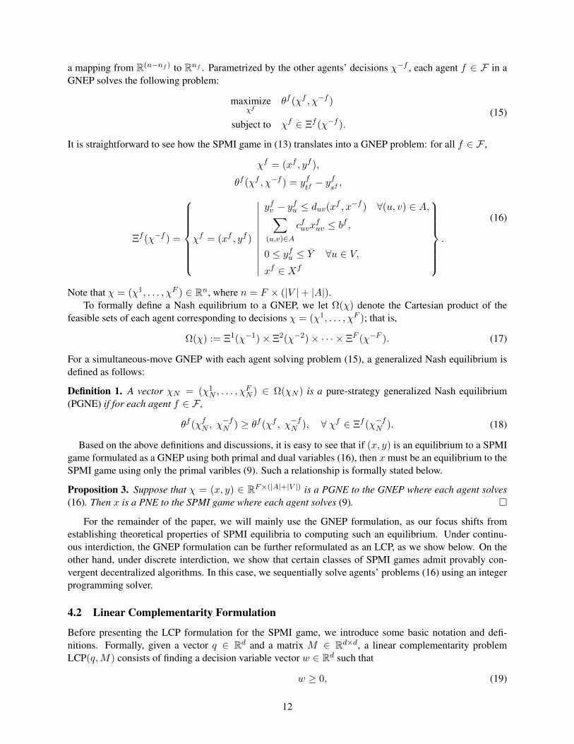
a mapping from R(n−nf ) to Rnf . Parametrized by the other agents’ decisions χ−f , each agent f ∈ F in aGNEP solves the following problem:

maximizeχf

θf (χf , χ−f )

subject to χf ∈ Ξf (χ−f ).(15)

It is straightforward to see how the SPMI game in (13) translates into a GNEP problem: for all f ∈ F ,

χf = (xf , yf ),

θf (χf , χ−f ) = yftf− yf

sf,

Ξf (χ−f ) =

χf = (xf , yf )

∣∣∣∣∣∣∣∣∣∣∣∣

yfv − yfu ≤ duv(xf , x−f ) ∀(u, v) ∈ A,∑(u,v)∈A

cfuvxfuv ≤ bf ,

0 ≤ yfu ≤ Y ∀u ∈ V,xf ∈ Xf

.

(16)

Note that χ = (χ1, . . . , χF ) ∈ Rn, where n = F × (|V |+ |A|).To formally define a Nash equilibrium to a GNEP, we let Ω(χ) denote the Cartesian product of the

feasible sets of each agent corresponding to decisions χ = (χ1, . . . , χF ); that is,

Ω(χ) := Ξ1(χ−1)× Ξ2(χ−2)× · · · × ΞF (χ−F ). (17)

For a simultaneous-move GNEP with each agent solving problem (15), a generalized Nash equilibrium isdefined as follows:

Definition 1. A vector χN = (χ1N , . . . , χ

FN ) ∈ Ω(χN ) is a pure-strategy generalized Nash equilibrium

(PGNE) if for each agent f ∈ F ,

θf (χfN , χ−fN ) ≥ θf (χf , χ−fN ), ∀ χf ∈ Ξf (χ−fN ). (18)

Based on the above definitions and discussions, it is easy to see that if (x, y) is an equilibrium to a SPMIgame formulated as a GNEP using both primal and dual variables (16), then x must be an equilibrium to theSPMI game using only the primal varibles (9). Such a relationship is formally stated below.

Proposition 3. Suppose that χ = (x, y) ∈ RF×(|A|+|V |) is a PGNE to the GNEP where each agent solves(16). Then x is a PNE to the SPMI game where each agent solves (9).

For the remainder of the paper, we will mainly use the GNEP formulation, as our focus shifts fromestablishing theoretical properties of SPMI equilibria to computing such an equilibrium. Under continu-ous interdiction, the GNEP formulation can be further reformulated as an LCP, as we show below. On theother hand, under discrete interdiction, we show that certain classes of SPMI games admit provably con-vergent decentralized algorithms. In this case, we sequentially solve agents’ problems (16) using an integerprogramming solver.

4.2 Linear Complementarity Formulation

Before presenting the LCP formulation for the SPMI game, we introduce some basic notation and defi-nitions. Formally, given a vector q ∈ Rd and a matrix M ∈ Rd×d, a linear complementarity problemLCP(q,M) consists of finding a decision variable vector w ∈ Rd such that

w ≥ 0, (19)

12

q +Mw ≥ 0, (20)

wT (q +Mw) = 0. (21)

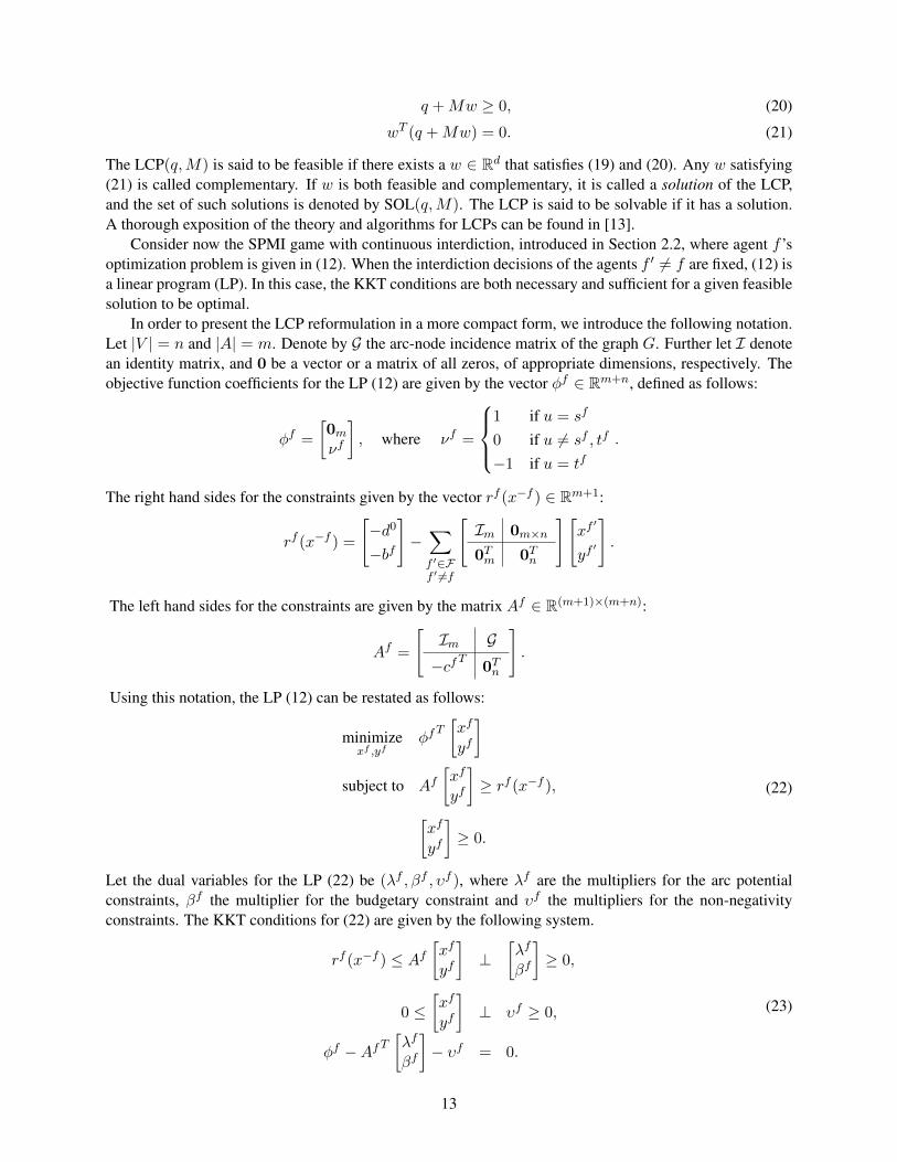
The LCP(q,M) is said to be feasible if there exists a w ∈ Rd that satisfies (19) and (20). Any w satisfying(21) is called complementary. If w is both feasible and complementary, it is called a solution of the LCP,and the set of such solutions is denoted by SOL(q,M). The LCP is said to be solvable if it has a solution.A thorough exposition of the theory and algorithms for LCPs can be found in [13].

Consider now the SPMI game with continuous interdiction, introduced in Section 2.2, where agent f ’soptimization problem is given in (12). When the interdiction decisions of the agents f ′ 6= f are fixed, (12) isa linear program (LP). In this case, the KKT conditions are both necessary and sufficient for a given feasiblesolution to be optimal.

In order to present the LCP reformulation in a more compact form, we introduce the following notation.Let |V | = n and |A| = m. Denote by G the arc-node incidence matrix of the graph G. Further let I denotean identity matrix, and 0 be a vector or a matrix of all zeros, of appropriate dimensions, respectively. Theobjective function coefficients for the LP (12) are given by the vector φf ∈ Rm+n, defined as follows:

φf =

[0mνf

], where νf =

1 if u = sf

0 if u 6= sf , tf

−1 if u = tf.

The right hand sides for the constraints given by the vector rf (x−f ) ∈ Rm+1:

rf (x−f ) =

[−d0

−bf

]−∑f ′∈Ff ′ 6=f

[Im 0m×n

0Tm 0Tn

][xf′

yf′

].

The left hand sides for the constraints are given by the matrix Af ∈ R(m+1)×(m+n):

Af =

[Im G−cf T 0Tn

].

Using this notation, the LP (12) can be restated as follows:

minimizexf ,yf

φfT[xf

yf

]subject to Af

[xf

yf

]≥ rf (x−f ),[

xf

yf

]≥ 0.

(22)

Let the dual variables for the LP (22) be (λf , βf , υf ), where λf are the multipliers for the arc potentialconstraints, βf the multiplier for the budgetary constraint and υf the multipliers for the non-negativityconstraints. The KKT conditions for (22) are given by the following system.

rf (x−f ) ≤ Af[xf

yf

]⊥

[λf

βf

]≥ 0,

0 ≤[xf

yf

]⊥ υf ≥ 0,

φf −Af T[λf

βf

]− υf = 0.

(23)

13

The KKT system (23) can be rewritten in the following form:

υf = φf −Af T[λf

βf

]≥ 0,

[xf

yf

]≥ 0,

[xf

yf

]Tυf = 0,

tf = −rf (x−f ) +Af[xf

yf

]≥ 0,

[λf

βf

]≥ 0, tf

T[λf

βf

]= 0.

(24)

In this form, it is easy to recognize that for a fixed value of x−f , the KKT system is equivalent to theLCP(qf (x−f ),Mf ) where

qf (x−f ) =

[φf

−rf (x−f )

]and Mf =

[0(m+n)×(m+n) −Af T

Af 0(m+1)×(m+1)

]. (25)

The decision variable vector for the LCP is the vector of combined decision variables wf :=(xf , yf , λf , βf )T . Each agent’s KKT system (24) is parametrized by the collective decisions of other agents.

Now by stacking all agents’ KKT systems together, the resulting model is itself an LCP, which can beseen from the following algebraic manipulation. First, consider the following system obtained from (24) byexpanding rf (x−f ):

υf = φf −Af T[λf

βf

]≥ 0,

[xf

yf

]≥ 0,

[xf

yf

]Tυf = 0,

tf =

[d0

bf

]+Af

[xf

yf

]+∑f ′∈Ff ′ 6=f

[Im 0m×n

0Tm 0Tn

][xf′

yf′

]≥ 0,

[λf

βf

]≥ 0, tf

T

[λf

βf

]= 0.

(26)

Now introduce a matrix Mf to represent the interactions between agent f ’s decision variables (xf , yf ) andthe KKT system of all the other agents, which has the following specific form:

Mf =

0m×m 0m×n 0m×m 0m×1

0n×m 0n×n 0n×m 0n×1

Im 0m×n 0m×m 0m×1

01×m 01×n 01×m 0

. (27)

Using this notation, the stacked KKT system (26) for agents f = 1, . . . , F can be formulated as anLCP(q,M), with the vector q and matrix M given as follows:

q = (q1, q2, . . . , qF )T , where qf = (φf , d0, bf )T , (28)

and

M =

M1 M2 M3 · · · MF

M1 M2 M3 · · · MF

......

......

...

M1 M2 · · · MF−1 MF

. (29)

Due to the equivalence between an agent f ’s optimization problem (12) and its KKT system (24), the aboveLCP(q,M) is equivalent to the corresponding (continuous) SPMI game in the sense that a candidate point(χ1, χ2, . . . , χF ), where χf = (xf , yf ), is an equilibrium to the SPMI game if and only if there existassociated Lagrangian multipliers such that they together solve the LCP(q,M).

14

Methods for solving LCPs fall broadly into two categories: (i) pivotal methods such as Lemke’s algo-rithm, and (ii) iterative methods such as splitting schemes and interior point methods. The former class ofmethods are finite when applicable, while the latter class converge to solutions in the limit. In general, theapplicability of these algorithms depends on the structural properties of the matrix M . In the followinganalysis, we show that LCP(q,M) for the SPMI game, as defined in (28) and (29), possesses two prop-erties that allow us to use Lemke’s pivotal algorithm: (i) the matrix M is a copositive matrix, and (ii)q ∈ (SOL(0,M))∗.1

We first show thatM is copositive. Recall that a matrixM ∈ Rd×d is said to be copositive if xTMx ≥ 0for all x ∈ Rd+.

Lemma 1. M defined as in (29) is copositive.

Proof. Let w ∈ R2m+n+1+ . Using the block structure of M given in (29), wTMw can be decomposed as

follows.

wTMw =

F∑f=1

wfTMfwf +

F∑f=1

F∑f ′=1f ′ 6=f

wfTMf ′wf

′. (30)

We analyze the terms in the two summations separately. First consider wf TMfwf for any agent f . Let thedual variables (λf , βf ) be collectively denoted by δf . We have

wfTMfwf =

[χf

TδfT] [

0 −Af T

Af 0

] [χf

δf

]= −χf TAf T δf + δf

TAfχf = 0.

(31)

Now consider any term of the form wfTMf ′wf

′:

wfTMf ′wf

′=

[xf

Tyf

Tλf

Tβf

T]

0 0 0 0

0 0 0 0

Im 0 0 0

0 0 0 0

xf′

yf′

λf′

βf′

=[xf

Tyf

Tλf

Tβf]

00

xf′

0

= λfTxf′.

(32)

Combining (31) and (32) we obtain

wTMw =F∑f=1

F∑f ′=1f ′ 6=f

λfTxf′. (33)

Since λf ’s and xf′’s are the elements of w, w ≥ 0 clearly implies that wTMw ≥ 0.

We now show that q ∈ (SOL(0,M))∗.

Lemma 2. Let the vector q and the matrix M be as defined in (28) and (29) respectively. Then q ∈(SOL(0,M))∗.

1Given a set K ∈ Rd, the set K∗ denotes the dual cone of K; i.e. K∗ = y ∈ Rd : yTx ≥ 0, ∀x ∈ K.

15

Proof. First note that SOL(0,M) 6= ∅ for any M , since 0 is always a solution to LCP(0,M). Now considera w ∈ SOL(0,M); i.e. 0 ≤ w ⊥ 0 + Mw ≥ 0. We prove that qTw ≥ 0. Observe that qTw can bedecomposed as follows:

qTw =F∑f=1

qfTwf =

F∑f=1

(φf

T

[xf

yf

]+ d0T λf + bfβf

)

=

F∑f=1

[(yfsf− yf

tf) + d0T λf + bfβf

].

(34)

The last two terms in the last equality above, d0T λf and bfβf , are non-negative for f = 1, . . . F becausew ∈ SOL(0,M) implies that λf , βf ≥ 0, and by assumption d0, bf ≥ 0 for each f = 1, . . . , F .

Now we focus on the first term in the last equality of (34):∑F

f=1(yfsf− yf

tf). First since Mw ≥ 0,

wf must solve the system (26) for f = 1, . . . , F , with φf , d0 and bf all set at 0 (as φf , d0 and bf are thecomponents of the vector q in the LCP(q,M), as defined in (28); and in LCP(0,M), q = 0). In this case,considering the primal feasibility of wf , we obtain the following:∑

a∈Acfax

fa ≤ 0

yfu − yfv +

F∑f=1

xfu,v ≥ 0 ∀(u, v) ∈ A

for f = 1, . . . , F. (35)

Recall that cfa ≥ 0 for all a ∈ A and f = 1, . . . , F by assumption. Therefore, (35) implies that xf = 0 forany agent f . It is easy to see that in this case, we must have

yfu − yfv ≥ 0 ∀(u, v) ∈ A, for f = 1, . . . F. (36)

Now consider any sf -tf path p. By assumption, there must be at least one such path for each agent f . Bysumming up the inequalities (36) over the arcs in the path p, we obtain the desired result. In other words,∑

(u,v)∈p

yfu − yfv = yfsf− yf

tf≥ 0. (37)

Summing up over the agents, we thus have shown that qTw ≥ 0 for any w ∈ SOL(0, M).

With Lemma 1 and 2, we can apply the following result from Cottle et al. [13].

Theorem 1 ( [13], Theorem 4.4.13). If M is copositive and q ∈ (SOL(0,M))∗, then Lemke’s method willalways compute a solution, if the problem is nondegenerate.2

As discussed earlier, the LCP approach is not applicable for discrete SPMI games due to the lack ofnecessary and sufficient optimality conditions. In the following we develop a decentralized approach thatworks for both discrete and continuous SPMI games.

2When the LCP is degenerate, cycling in Lemke’s method can indeed occur, as shown in Section 4.9 of [13]. However, asindicated in Eaves [16], when ambiguity arises in choosing the index to exit the basis, just randomly choose an index to leave thebasis. The finite convergence of the Lemke’s method still holds.

16

4.3 Gauss-Seidel Algorithm (Algorithm 1)

We first present the basic form of a best response based algorithm. The idea is simple: starting with aparticular feasible decision vector χ0 = (χ1

0, χ20, . . . , χ

F0 ) ∈ Ω(χ0), solve the optimization problem of a

particular agent, say, agent 1, with all of the other agents’ actions fixed. Assume an optimal solution existsto this optimization problem, and denote it as χ1∗

1 . The next agent, say, agent 2, solves its own optimizationproblem, with the other agents’ actions fixed as well, but with χ1

0 replaced by χ1∗1 . Such an approach is often

referred to as a diagonalization scheme or a Gauss-Seidel iteration, and for the remainder of this paper weuse the latter name to refer to this simple best-response approach.

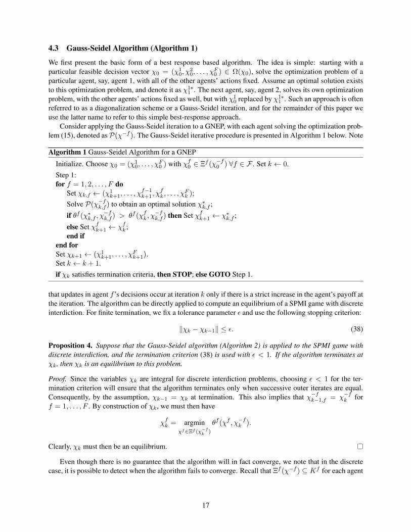
Consider applying the Gauss-Seidel iteration to a GNEP, with each agent solving the optimization prob-lem (15), denoted as P(χ−f ). The Gauss-Seidel iterative procedure is presented in Algorithm 1 below. Note

Algorithm 1 Gauss-Seidel Algorithm for a GNEP

Initialize. Choose χ0 = (χ10, . . . , χ

F0 ) with χf0 ∈ Ξf (χ−f0 ) ∀f ∈ F . Set k ← 0.

Step 1:for f = 1, 2, . . . , F do

Set χk,f ← (χ1k+1, . . . , χ

f−1k+1, χ

fk , . . . , χ

Fk );

Solve P(χ−fk,f ) to obtain an optimal solution χ∗k,f ;

if θf (χ∗k,f , χ−fk,f ) > θf (χfk , χ

−fk,f ) then Set χfk+1 ← χ∗k,f ;

else Set χfk+1 ← χfk ;end if

end forSet χk+1 ← (χ1

k+1, . . . , χFk+1).

Set k ← k + 1.

if χk satisfies termination criteria, then STOP; else GOTO Step 1.

that updates in agent f ’s decisions occur at iteration k only if there is a strict increase in the agent’s payoff atthe iteration. The algorithm can be directly applied to compute an equilibrium of a SPMI game with discreteinterdiction. For finite termination, we fix a tolerance parameter ε and use the following stopping criterion:

‖χk − χk−1‖ ≤ ε. (38)

Proposition 4. Suppose that the Gauss-Seidel algorithm (Algorithm 2) is applied to the SPMI game withdiscrete interdiction, and the termination criterion (38) is used with ε < 1. If the algorithm terminates atχk, then χk is an equilibrium to this problem.

Proof. Since the variables χk are integral for discrete interdiction problems, choosing ε < 1 for the ter-mination criterion will ensure that the algorithm terminates only when successive outer iterates are equal.Consequently, by the assumption, χk−1 = χk at termination. This also implies that χ−fk−1,f = χ−fk forf = 1, . . . , F . By construction of χk, we must then have

χfk = argminχf∈Ξf (χ−f

k )

θf (χf , χ−fk ).

Clearly, χk must then be an equilibrium.

Even though there is no guarantee that the algorithm will in fact converge, we note that in the discretecase, it is possible to detect when the algorithm fails to converge. Recall that Ξf (χ−f ) ⊆ Kf for each agent

17

f ∈ F , where Kf is defined below.

Kf =

(xf , yf )

∣∣∣∣∣∑

(u,v)∈V

cfuvxfuv ≤ bf ,

0 ≤ yfu ≤ Y ∀u ∈ V

. (39)

Clearly, the set∏Ff=1K

f is finite. Any intermediate point χk generated by Algorithm 2 must certainly

satisfy the budgetary constraints on xfk and the bound constraints on yfk for each agent f . Therefore χk ∈∏Ff=1K

f . In other words, the set of possible points χk generated by Algorithm 2 lies in a finite set. Thismeans that if the algorithm fails to converge, it must generate a sequence that contains at least one cycle.The existence of such cycles in non-convergent iterate paths can then be used to detect situations in whichthe algorithm fails to converge.

Proposition 4 is likely the best one can do for general SPMI games under discrete interdiction. However,for the subclass of such games with common source-target pairs, we can in fact prove that the best responsedynamics always terminates in a NE in a finite number of steps.

Proposition 5. Consider a SPMI game with discrete interdiction with common source-target pairs, andassume that the initial arc lengths d and arc extensions e are integral. Suppose that Algorithm 2 is appliedto such a problem, and the termination criteria (38) is used with ε < 1. Then the algorithm will terminatefinitely at an equilibrium.

Proof. Denote the common source node as s, and the common target node as t. The set of joint feasiblestrategies in x under the given assumptions is a finite set. Moreover, all the agents attempt to minimizethe common objective, namely the s-t path length. Note that at any iteration k at which an update occursfor any agent’s decision, there must then be a strict increase in the s-t path length. Thus there cannot existcycles in the sequence χk. Furthermore, since the set of joint feasible strategies is finite, the sequencemust terminate at some point χ∗. It is easy to show that χ∗ must be an equilibrium (cf. Proposition 4).

4.4 Regularized Gauss-Seidel Algorithm (Algorithm 2)

One disadvantage of the “naıve” Gauss-Seidel algorithm described above is that for continuous GNEPs, itcan fail to converge to an equilibrium. However, Facchinei et al. [21] showed that under certain assumptions,we can overcome this issue by adding a regularization term to the individual agent’s problem solved in aGauss-Seidel iteration.

The regularized version of the optimization problem for agent f ∈ F is

maximizeχf

θf (χf , χ−f )− τ∥∥∥χf − χf∥∥∥2

subject to χf ∈ Ξf (χ−f ),

(40)

where τ is a positive constant. Here the regularization term is evaluated in relation to a candidate pointχf . Note that the point χf and the other agents’ decision variables χ−f are fixed when the problem (40) issolved. We refer to problem (40) as R(χ−f , χf ). The regularized Gauss-Seidel procedure, herein referredto as Algorithm 2, is simply Algorithm 1, except that R(χ−fk,f , χ

fk) is solved in each iteration k instead of

P(χ−fk,f ).This version of the algorithm, along with its convergence proof, was originally presented in [21] to solve

GNEPs with shared constraints. The difficulty here that prevents us from showing convergence lies in thefact that we are dealing with GNEPs with non-shared constraints. As a result, any intermediate points re-sulting from an agent’s best responses need not to be feasible in the other agents’ problems. Consequently,

18

Algorithm 2 Gauss-Seidel Algorithm for a GNEP

Initialize. Choose χ0 = (χ10, . . . , χ

F0 ) with χf0 ∈ Ξf (χ−f0 ) ∀f ∈ F . Set k ← 0.

Step 1:for f = 1, 2, . . . , F do

Set χk,f ← (χ1k+1, . . . , χ

f−1k+1, χ

fk , . . . , χ

Fk );

SolveR(χ−fk,f , χfk) to obtain an optimal solution χ∗k,f ;

Set χfk+1 ← χ∗k,f ;end forSet χk+1 ← (χ1

k+1, . . . , χFk+1).

Set k ← k + 1.

if χk satisfies termination criteria, then STOP; else GOTO Step 1.

we use Algorithm 2 only as a heuristic algorithm to solve SPMI games under continuous interdiction. Nev-ertheless, we can show that if Algorithm 2 converges, then the resulting point is an equilibrium to the SPMIgame.

Proposition 6. Let χk be the sequence generated by applying Algorithm 2 to the SPMI problem undercontinuous interdiction, wherein each agent solves the regularized version of (13). Suppose χk convergesto χ. Then χ is an equilibrium to the SPMI problem.

The proof of this proposition is almost identical to that of Theorem 4.3 in Facchinei et al. [21]. However,we do want to point out one key difference in the proof. In Proposition 6, we need to assume that theentire sequence χk converges to χ. This is a strong assumption in the sense that it also requires thatall the intermediate points χk,f in Algorithm 2 to converge to χ, a fact key to proving that χ is indeed anequilibrium. In contrast, for GNEPs with shared constraints, this assumption may be weakened becausethe intermediate points χk,f and therefore the cluster points of the sequence generated by the algorithm areguaranteed to be feasible. The complete proof is presented in Appendix A.

Similar to discrete SPMI games, the convergence of Algorithm 2 is guaranteed for continuous-interdiction SPMI games with common source-target pairs. The key fact that allows us to prove this strongerresult is that by dropping the dependence of the variables y on the agents f ∈ F , any unilateral deviation inthe shared variables y results in a solution that remains feasible in the other agents’ optimization problems.The convergence result is formally stated below.

Proposition 7. Consider applying Algorithm 2 to the SPMI problem under continuous interdiction withcommon source-target pairs, where each agent solves the regularized version of (13). Let χk be thesequence generated by the algorithm. If χ is a cluster point of this sequence, then it also solves the SPMIproblem.

5 Numerical Results

We use the algorithms presented in the previous section to study several instances of SPMI games. Thedecentralized algorithms were implemented in MATLAB R2010a with CPLEX v12.2 as the optimizationsolver. The LCP formulation for the SPMI game with continuous interdiction was solved using the MAT-LAB interface for the complementarity solver PATH [22]. Computational experiments were carried out ona desktop workstation with a quad-core Intel Core i7 processor and 16 GHz of memory running Windows 7.

In the implementation of the decentralized algorithm, for SPMI games with discrete interdiction, weused Algorithm 2 with τ = 0. For SPMI games with continuous interdiction, we followed a strategy oftrying the “naıve” Gauss-Seidel algorithm – i.e. Algorithm 2 with τ = 0 – first. If this version failed to

19

converge in 1000 outer iterations, we then set τ to a strictly positive value and used the more expensiveregularized Gauss-Seidel algorithm.

Computing Equilibria

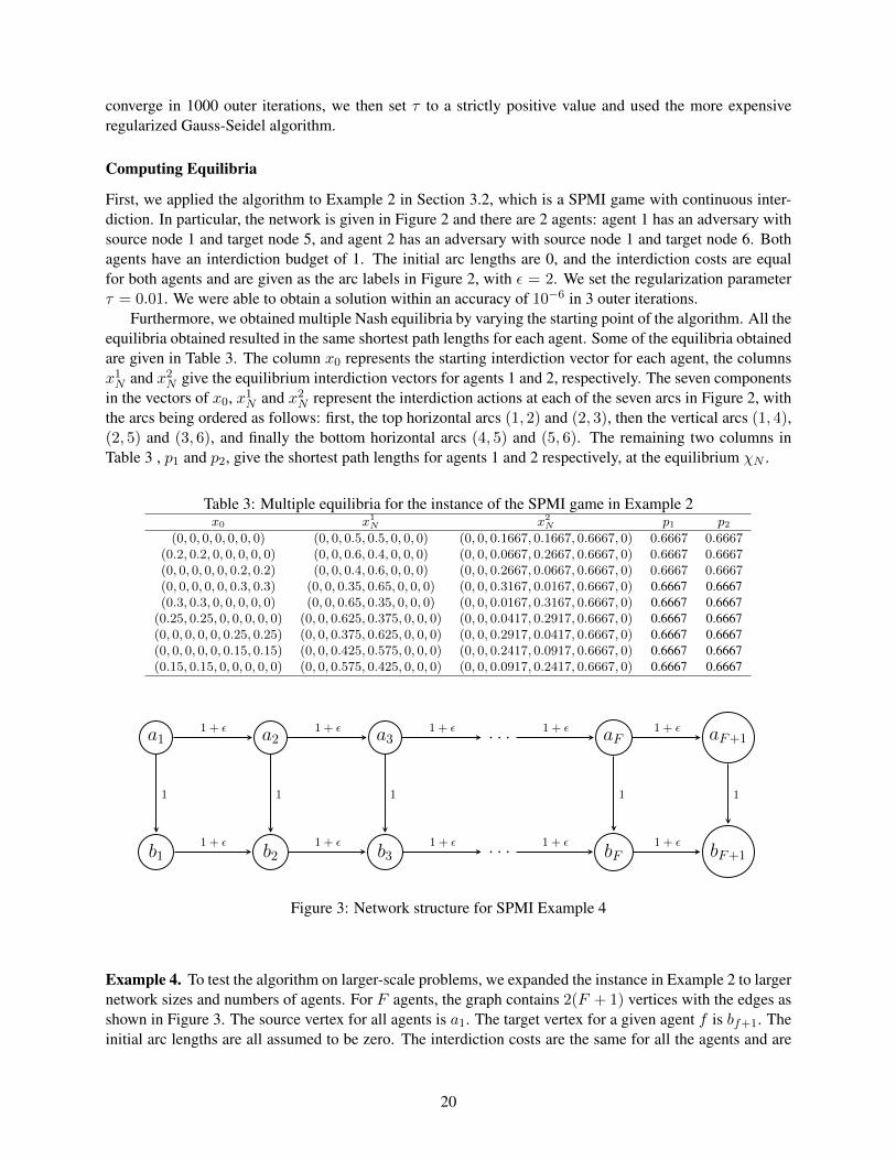
First, we applied the algorithm to Example 2 in Section 3.2, which is a SPMI game with continuous inter-diction. In particular, the network is given in Figure 2 and there are 2 agents: agent 1 has an adversary withsource node 1 and target node 5, and agent 2 has an adversary with source node 1 and target node 6. Bothagents have an interdiction budget of 1. The initial arc lengths are 0, and the interdiction costs are equalfor both agents and are given as the arc labels in Figure 2, with ε = 2. We set the regularization parameterτ = 0.01. We were able to obtain a solution within an accuracy of 10−6 in 3 outer iterations.

Furthermore, we obtained multiple Nash equilibria by varying the starting point of the algorithm. All theequilibria obtained resulted in the same shortest path lengths for each agent. Some of the equilibria obtainedare given in Table 3. The column x0 represents the starting interdiction vector for each agent, the columnsx1N and x2

N give the equilibrium interdiction vectors for agents 1 and 2, respectively. The seven componentsin the vectors of x0, x1

N and x2N represent the interdiction actions at each of the seven arcs in Figure 2, with

the arcs being ordered as follows: first, the top horizontal arcs (1, 2) and (2, 3), then the vertical arcs (1, 4),(2, 5) and (3, 6), and finally the bottom horizontal arcs (4, 5) and (5, 6). The remaining two columns inTable 3 , p1 and p2, give the shortest path lengths for agents 1 and 2 respectively, at the equilibrium χN .

Table 3: Multiple equilibria for the instance of the SPMI game in Example 2x0 x1

N x2N p1 p2

(0, 0, 0, 0, 0, 0, 0) (0, 0, 0.5, 0.5, 0, 0, 0) (0, 0, 0.1667, 0.1667, 0.6667, 0) 0.6667 0.6667(0.2, 0.2, 0, 0, 0, 0, 0) (0, 0, 0.6, 0.4, 0, 0, 0) (0, 0, 0.0667, 0.2667, 0.6667, 0) 0.6667 0.6667(0, 0, 0, 0, 0, 0.2, 0.2) (0, 0, 0.4, 0.6, 0, 0, 0) (0, 0, 0.2667, 0.0667, 0.6667, 0) 0.6667 0.6667(0, 0, 0, 0, 0, 0.3, 0.3) (0, 0, 0.35, 0.65, 0, 0, 0) (0, 0, 0.3167, 0.0167, 0.6667, 0) 0.6667 0.6667(0.3, 0.3, 0, 0, 0, 0, 0) (0, 0, 0.65, 0.35, 0, 0, 0) (0, 0, 0.0167, 0.3167, 0.6667, 0) 0.6667 0.6667

(0.25, 0.25, 0, 0, 0, 0, 0) (0, 0, 0.625, 0.375, 0, 0, 0) (0, 0, 0.0417, 0.2917, 0.6667, 0) 0.6667 0.6667(0, 0, 0, 0, 0, 0.25, 0.25) (0, 0, 0.375, 0.625, 0, 0, 0) (0, 0, 0.2917, 0.0417, 0.6667, 0) 0.6667 0.6667(0, 0, 0, 0, 0, 0.15, 0.15) (0, 0, 0.425, 0.575, 0, 0, 0) (0, 0, 0.2417, 0.0917, 0.6667, 0) 0.6667 0.6667(0.15, 0.15, 0, 0, 0, 0, 0) (0, 0, 0.575, 0.425, 0, 0, 0) (0, 0, 0.0917, 0.2417, 0.6667, 0) 0.6667 0.6667

a1 a2 a3 . . . aF aF+1

b1 b2 b3 . . . bF bF+1

1 + ǫ 1 + ǫ

1 + ǫ 1 + ǫ

1 1 1

1 + ǫ 1 + ǫ 1 + ǫ

1 + ǫ 1 + ǫ 1 + ǫ

1 1

Figure 3: Network structure for SPMI Example 4

Example 4. To test the algorithm on larger-scale problems, we expanded the instance in Example 2 to largernetwork sizes and numbers of agents. For F agents, the graph contains 2(F + 1) vertices with the edges asshown in Figure 3. The source vertex for all agents is a1. The target vertex for a given agent f is bf+1. Theinitial arc lengths are all assumed to be zero. The interdiction costs are the same for all the agents and are

20

given as the arc labels in Figure 3. All the agents have an interdiction budget of 1. The cost parameter ε ischosen as 2. For discrete interdiction on these graphs, the arc extensions are assumed to be length 1.

The running time and iterations required to compute equilibria for these instances are summarized inTable 4. The first four columns in the table give the number of outer iterations and runtime for Algorithm 2over these instances with continuous interdiction. The results indicate that the running time for the central-ized Lemke’s method increases monotonically with the problem size. However, the running time for thedecentralized method depends not just on the problem size but also on the number of outer iterations. Ingeneral, there is no correlation between these two parameters. Indeed the algorithm is observed to convergein relatively few iterations even for some large problem instances. This is in stark contrast to the rapidincrease in running time observed for the LCP approach as problem size increases.

It must be noted that the order in which the individual agent problems are solved in the Gauss-Seidelalgorithm plays an important role. Indeed, the algorithm failed to converge for certain orderings of theagents, but succeeded in finding equilibria quickly for the same instance with other orderings. For instance,for a network of size 25, solving the agent problems in their natural order 1, 2, . . . , 25 resulted in thefailure of the “naıve” version of the algorithm to converge even after 1000 outer iterations. However, witha randomized agent order, the algorithm converged in as few as 13 iterations. It is encouraging to note thatfor the same agent order that resulted in the failure of the naive version, the regularized method convergedto a GNE within 394 outer-iterations with a runtime of 28 wall-clock seconds.

Table 4: Number of iterations and running times for SPMI Example 4.Continuous Interdiction Discrete Interdiction

Decentralized LCP Decentralized# Agents # Iters Runtime (s) Runtime (s) # Iters Runtime (s)

5 3 0.0205 0.0290 5 0.177610 5 0.0290 0.1833 3 0.162715 11 0.1103 0.7534 3 0.241920 5 0.0723 2.1106 3 0.316425 13 0.2609 4.8167 3 0.400530 15 0.4070 10.2256 3 0.515535 10 0.3605 17.7387 3 0.594840 41 1.7485 30.2382 3 0.738745 12 0.6601 48.6280 3 0.879450 12 0.7981 75.0420 3 1.0385

Computation of Efficiency Losses

Using the decentralized algorithm and its potential to find multiple equilibria by starting at different points,we numerically study the efficiency loss of decentralized interdiction strategies in SPMI games. We focusfirst on Example 4, with the underlying network represented in Figure 3. We first show that in general,the worst-case price of anarchy cannot be bounded from above. We do so by demonstrating that given anycandidate upper bound on the worst-case price of anarchy, we can construct an instance that invalidates thebound.

Consider the specific instance of the problem as depicted in Figure 3. Recall that there are F agentsand the source-target pair for agent f is (a1, bf+1). Note that all paths for all agents contain either thearc (a1, a2) or the arc (a1, b1). Then one feasible solution to the centralized problem is for each agent tointerdict both these arcs by 1/(2 + ε) for a total cost of 1. In this case, the length of both arcs becomeF/(2 + ε), giving a shortest path length of F/(2 + ε) for each agent. Note that this is not an equilibrium

21

solution as agent 1 can deviate unilaterally to interdict arcs (a1, b1) and (a2, b2) by 1/2 to obtain a shortestpath length of (F + ε/2)/(2 + ε).

A Nash equilibrium to this instance is given by the following solution. Agent f interdicts the verticalarcs (a1, b1), . . . , (af , bf ) by 1/(f(f + 1)) and the arc (af+1, bf+1) by f/(f + 1). Each agent then hasa shortest path length of F/(F + 1). Note that all the sf -tf paths are of equal length for every agent.Therefore diverting any of the budget to any vertical arcs will result in unequal path lengths and a shortershortest path for any agent. Obviously, diverting the budget to interdict any of the horizontal arcs is costinefficient because of their higher interdiction cost at 1 + ε. Thus no agent has an incentive to deviate fromthis solution.

We now have a feasible solution to the centralized problem that has an objective value of F/(2 + ε) foreach agent, and a Nash equilibrium that has an objective value of F/(F + 1) for each agent. Therefore, byits definition in (4), the worst-case price of anarchy for the SPMI game depicted in Figure 3 must be at least(F + 1)/(2 + ε).

The observation above implies that given any fixed candidate upper bound on the worst-case price ofanarchy for the general class of SPMI games, under continuous interdiction, we can easily compute a tuple(F, ε), which gives us an instance of the problem that breaks the bound.

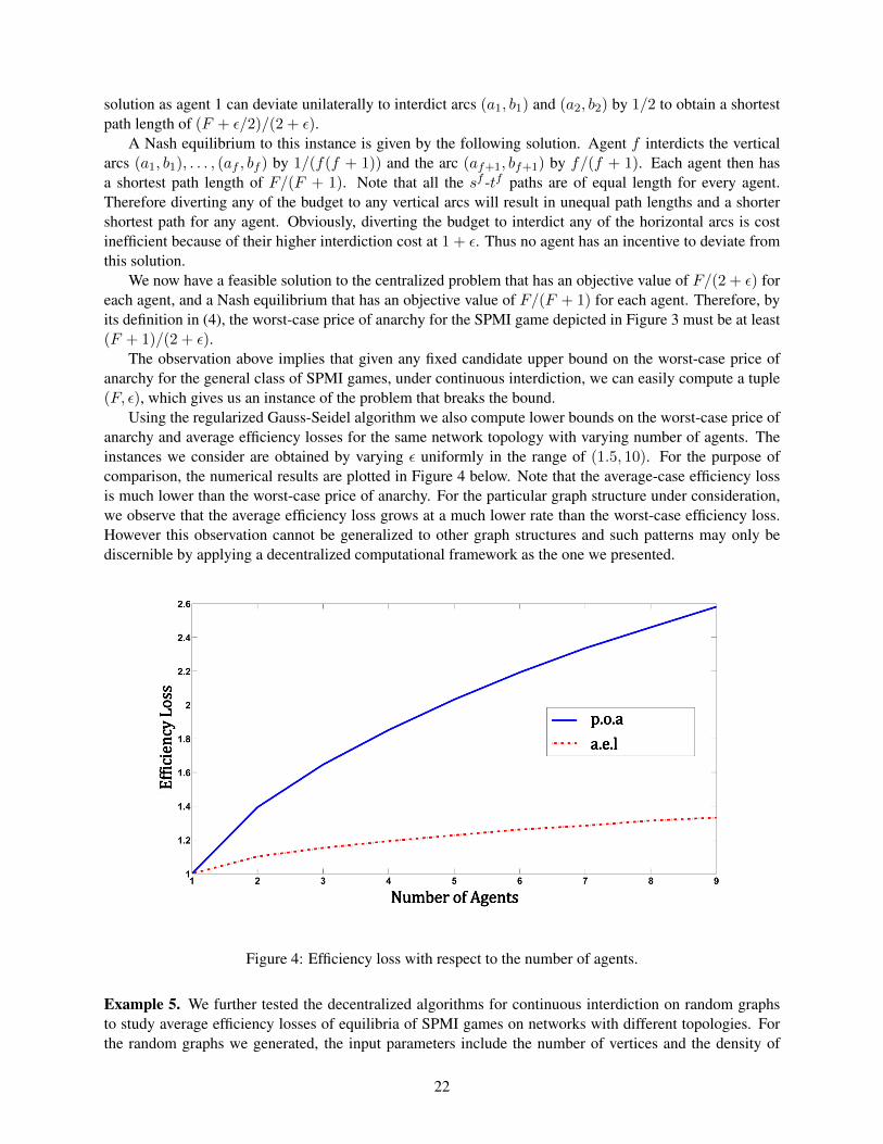
Using the regularized Gauss-Seidel algorithm we also compute lower bounds on the worst-case price ofanarchy and average efficiency losses for the same network topology with varying number of agents. Theinstances we consider are obtained by varying ε uniformly in the range of (1.5, 10). For the purpose ofcomparison, the numerical results are plotted in Figure 4 below. Note that the average-case efficiency lossis much lower than the worst-case price of anarchy. For the particular graph structure under consideration,we observe that the average efficiency loss grows at a much lower rate than the worst-case efficiency loss.However this observation cannot be generalized to other graph structures and such patterns may only bediscernible by applying a decentralized computational framework as the one we presented.

Figure 4: Efficiency loss with respect to the number of agents.

Example 5. We further tested the decentralized algorithms for continuous interdiction on random graphsto study average efficiency losses of equilibria of SPMI games on networks with different topologies. Forthe random graphs we generated, the input parameters include the number of vertices and the density of

22

a graph, which is the number of arcs divided by the maximum possible number of arcs. The number ofagents was chosen randomly from the interval (0, |V |/2), and one such number is chosen per vertex setsize. Source-target pairs were chosen at random for each interdictor. Fixing the vertex set, we populated thearc set by successively generating source-target paths for the agents until the desired density was reached.We thus ensured connectivity between the source-target pairs for each agent. Costs, initial arc lengthsand interdiction budgets were chosen from continuous uniform distributions. Arc interdiction costs wereassigned uniformly in the range [1, 5]. The budget for each agent f was chosen uniformly from the interval[bf/10, bf/2], where bf =

∑a∈A c

fa . The initial length of each arc was chosen uniformly from [1, 5].

For each combination of vertex set size, the number of agents, and graph density, we generated 25 ran-dom instances by drawing values from the uniform distributions described above for the various networkparameters. For each instance, we used 10 different random permutations of the agents to run the decentral-ized algorithms in an attempt to compute multiple equilibria. The lower bound on the price of anarchy forthe game was computed as the worst case efficiency loss over these 25 instances. The average efficiency lossover these instances was also computed. The results are summarized in Table 5. Our experiments indicatethat the average efficiency loss and the worst-case price of anarchy tend to grow as the number of verticesand number of agents increases; on the other hand, these measures of efficiency loss sometimes do notappear to be monotonically increasing or decreasing with respect to the density of the underlying network.

Table 5: SPMI Continuous Interdiction - Random Graphs# Vertices # Agents Density Avg. Run Time (s) # Avg Iters. a.e.l p.o.a

5 3 0.25 0.0037 3 1.3133 1.55615 3 0.5 0.0038 3 1.3265 1.95295 3 0.75 0.0040 3 1.5099 2.3829

10 3 0.25 0.0065 4 1.5366 2.207810 3 0.5 0.0176 11 1.4538 2.311410 3 0.75 0.0132 8 1.4273 2.134215 4 0.25 0.0263 11 1.7091 2.924615 4 0.5 0.0939 33 1.7524 2.790415 4 0.75 0.1267 42 1.5695 2.142520 5 0.25 0.1269 34 2.1907 3.288520 5 0.5 0.2087 43 1.8523 2.790620 5 0.75 0.5416 100 1.7967 2.378225 7 0.25 0.7167 105 2.5631 4.878825 7 0.5 1.9564 207 2.3022 5.579425 7 0.75 1.8476 158 1.9884 2.4423

6 Conclusions and Future Work

In this work, we introduced decentralized multi-interdictor games and gave formulations for one such classof games – shortest path multi-interdictor games. We analyzed the theoretical properties of SPMI games: inparticular, we gave conditions for the existence of equilibria and examples where multiple equilibria exist.Specifically, we proved the existence of equilibria for general SPMI games under continuous interdiction.On the other hand, for the discrete counterpart, we provide an example where a pure-strategy equilibriumdoes not exist. However, for the subclass of problems with common source-target pairs, we are able toprovide an existence guarantee.

We also showed that the SPMI game under continuous interdiction is equivalent to a linear comple-mentarity problem, which can be solved by Lemke’s algorithm. This constitutes a convergent centralizedmethod to solve such problems. We also presented decentralized heuristic algorithms to solve SPMI gamesunder both continuous and discrete interdiction. Finally, we used these algorithms to numerically evaluatethe worst case and average efficiency loss of SPMI games.

23

There are other classes of network interdiction games that can be studied using the same frameworkwe have developed, where the agents’ obstruction functions are related to the maximum flow or minimumcost flow in the network. Establishing theoretical results and studying the applicability of the decentralizedalgorithms to other classes of decentralized network interdiction games are natural and interesting extensionsof this work.

In our study of SPMI games, we also made the assumption that the games have complete informationstructure; that is, the normal form of the game – the set of agents, agents’ feasible action spaces, and theirobjective functions – is assumed to be common knowledge to all agents. In addition, we made the implicitassumption that all input data are deterministic. However, data uncertainty and lack of observability of otheragents’ preferences or actions are prevalent in real-world situations. For such settings, we need to extendour work to accommodate games with exogenous uncertainties and incomplete information.

One might also be interested in designing interventions to reduce the loss of efficiency resulting fromdecentralized control. This leads to the topic of mechanism design. Such a line of work also defines a veryimportant and interesting future research direction.

Acknowledgement

This work was partially supported by the Air Force Office of Scientific Research (AFOSR) under grantFA9550-12-1-0275.

A Proof of Proposition 6

We prove the proposition in two steps. We first show that χ is feasible to each player’s problem. Since byassumption χk → χ, we must have χfk → χf and

limk→∞

∥∥∥χfk+1 − χfk

∥∥∥ = 0, ∀f ∈ F . (41)

By construction of χk,f , (41) implies that

limk→∞

χk,f = χ, ∀f ∈ F . (42)

Consider χk,f+1 = (χ1k+1, . . . , χ

fk+1, χ

f+1k , χFk ). By Step 1 of Algorithm 2, we must have

χfk+1 ∈ Ξf (χ−fk,f+1). (43)

Note that by (41) and (42), χfk+1 → χf and χ−fk,f+1 → χ−f . The set Ξf (χ−fk,f ) is defined by linear inequal-

ities parametrized by χ−fk,f . Thus we may utilize continuity properties of this set valued mapping, and takelimits on (43) to obtain

χf ∈ Ξf (χ−f ). (44)

In other words, χ is feasible for every agent’s optimization problem (15).We complete the proof by showing that for each agent f ∈ F

θf (χf , χ−f ) ≥ θf (χf , χ−f ), ∀ χf ∈ Ξf (χ−f ).

For the purpose of establishing a contradiction, suppose that there is an agent f and a vector ξf ∈ Ξf (χ−f )such that

θf (χf , χ−f ) < θf (ξf , χ−f ).

24

Let df = (ξf − χf ). Then by the subdifferentiality inequality for concave functions we must have

θ′f (χf , χ−f ; df ) > 0. (45)

Our proof relies on constructing a contradiction to (45). To do so, we first construct a sequence ξfk that is

feasible to agent f ’s problem at the k-th iteration, such that ξfk → ξf .Using the linearity of the functions that define the set valued mapping Ξf (·) we can show its inner

semicontinuity relative to its domain (cf. [38] Chapter 5). Because χ−f ∈ dom(Ξf (·)), we then have

lim infξ−f→χ−f

Ξ(ξ−f ) ⊇ Ξ(χ−f ), (46)

where the limit in (46) is given by the following:

lim infξ−f→χ−f

Ξ(ξ−f ) =uf | ∀ξ−fk → χ−f , ∃ufk → uf with ufk ∈ Ξf (ξ−fk )

. (47)

By assumption, ξf ∈ Ξf (χ−f ). By (42) we also have χ−fk,f → χ−f . Equation (47) then allows us to

construct a sequence ξfk ∈ Ξf (χ−fk,f ) such that ξfk → ξf as k →∞.Denote by Φf the regularized objective function for agent f ’s subproblem. In other words,

Φf (χf , χ−f , z) = θf (χf , χ−f )− τ∥∥∥χf − z∥∥∥2

.

We then haveΦ′f (χf , χ−f , z; df ) = θ′f (χf , χ−f ; df )− 2τ(χf − z)Tdf .

Note that χfk+1 is obtained by solving the problem R(χ−fk,f, χfk). In other words, χfk+1 maximizes

Φf (·, χ−fk,f, χfk) over the set Ξf (χ−f

k,f). Applying first order optimality conditions, setting z = χfk and

df = ξfk − χfk+1, we obtain the following.

Φ′f (χfk+1, χ−fk,f, χfk ; (ξfk − χ

fk+1)) = θ′f (χfk+1, χ

−fk,f

; (ξfk − χfk+1))

+ 2τ(χfk+1 − χfk)(ξfk − χ

fk+1)

≤ 0.

(48)

Passing to the limit k →∞, k ∈ K and using (42) we obtain

0 ≥ θ′f (χf , χ−f ; (ξf − χf )),

which contradicts (45).

References

[1] Russian warplanes disrupt ISIS oil sales channels; destroy 500 terrorist oil trucks in Syria. RT America,https://www.rt.com/news/322614-russian-warplanes-isis-oil-trucks/.Last edited: November 20, 2015.

[2] S. Albers, S. Eilts, E. Even-Dar, Y. Mansour, and L. Roditty. On Nash equilibria for a network creationgame. In Proceedings of the 17th Annual ACM-SIAM Symposium on Discrete Algorithms, pages 89–98. ACM, 2006.

25

[3] E. Anshelevich, A. Dasgupta, J. Kleinberg, E. Tardos, T. Wexler, and T. Roughgarden. The price ofstability for network design with fair cost allocation. SIAM Journal on Computing, 38(4):1602–1623,2008.

[4] N. Assimakopoulos. A network interdiction model for hospital infection control. Computers in Biologyand Medicine, 17(6):413–422, 1987.

[5] B. Awerbuch, Y. Azar, and A. Epstein. The price of routing unsplittable flow. In Proceedings of the37th Annual ACM Symposium on Theory of Computing, pages 57–66. ACM, 2005.

[6] M.S. Bazaraa, J.J. Jarvis, and H.D. Sherali. Linear Programming and Network Flows. Wiley, 2011.

[7] S. Boyd and L. Vandenberghe. Convex Optimization. Cambridge university press, 2004.

[8] G. Christodoulou and E. Koutsoupias. On the price of anarchy and stability of correlated equilibria oflinear congestion games. In Algorithms–ESA 2005, pages 59–70. Springer, 2005.

[9] R.L. Church, M.P. Scaparra, and R.S. Middleton. Identifying critical infrastructure: The medianand covering facility interdiction problems. Annals of the Association of American Geographers,94(3):491–502, 2004.

[10] R. Cole, Y. Dodis, and T. Roughgarden. How much can taxes help selfish routing? Journal of Computerand System Sciences, 72(3):444–467, 2006.

[11] J. Corbo and D. Parkes. The price of selfish behavior in bilateral network formation. In Proceedingsof the 24th Annual ACM Symposium on Principles of Distributed Computing, pages 99–107. ACM,2005.

[12] J.R. Correa, A.S. Schulz, and N.E. Stier-Moses. Selfish routing in capacitated networks. Mathematicsof Operations Research, 29(4):961–976, 2004.

[13] R.W. Cottle, J.S. Pang, and R.E. Stone. The Linear Complementarity Problem, volume 60. Society forIndustrial and Applied Mathematics, 2009.

[14] G. Debreu. A social equilibrium existence theorem. Proceedings of the National Academy of Sciencesof the United States of America, 38(10):886, 1952.

[15] A. Dreves, A. von Heusinger, C. Kanzow, and M. Fukushima. A globalized Newton method for thecomputation of normalized Nash equilibria. Journal of Global Optimization, 56(2):327–340, 2013.

[16] C. B Eaves. The linear complementarity problem. Management Science, 17(9):612–634, 1971.

[17] A. Fabrikant, A. Luthra, E. Maneva, C.H. Papadimitriou, and S. Shenker. On a network creation game.In Proceedings of the 22nd Annual ACM Symposium on Principles of Distributed Computing, pages347–351. ACM, 2003.

[18] F. Facchinei, A. Fischer, and V. Piccialli. On generalized Nash games and variational inequalities.Operations Research Letters, 35(2):159 – 164, 2007.

[19] F. Facchinei and C. Kanzow. Generalized Nash equilibrium problems. 4OR, 5(3):173–210, 2007.

[20] F. Facchinei and C. Kanzow. Penalty methods for the solution of generalized Nash equilibrium prob-lems. SIAM Journal on Optimization, 20(5):2228–2253, 2010.

[21] F. Facchinei, V. Piccialli, and M. Sciandrone. Decomposition algorithms for generalized potentialgames. Computational Optimization and Applications, 50:237–262, 2011.

26

[22] M. C. Ferris and T. S. Munson. Interfaces to path 3.0: Design, implementation and usage. Computa-tional Optimization and Applications, 12(1-3):207–227, 1999.

[23] M. Fukushima. Restricted generalized Nash equilibria and controlled penalty algorithm. Computa-tional Management Science, 8(3):201–218, 2011.

[24] P.M. Ghare, D.C. Montgomery, and W.C. Turner. Optimal interdiction policy for a flow network. NavalResearch Logistics Quarterly, 18(1):37–45, 1971.

[25] P.T. Harker. Generalized Nash games and quasi-variational inequalities. European Journal of Opera-tional Research, 54(1):81 – 94, 1991.

[26] G. Harris. U.S. and Russia agree on steps to combat ISIS in Syria. New York Times, http://nyti.ms/29EsoRt, July 15, 2016.

[27] E. Israeli and R.K. Wood. Shortest-path network interdiction. Networks, 40(2):97–111, 2002.

[28] R. Johari and J.N. Tsitsiklis. Efficiency loss in a network resource allocation game. Mathematics ofOperations Research, 29(3):407–435, 2004.

[29] R. Johari and J.N. Tsitsiklis. Efficiency of scalar-parameterized mechanisms. Operations Research,57(4):823–839, 2009.

[30] B.B.H. Korte and J. Vygen. Combinatorial Optimization: Theory and Algorithms. Algorithms andCombinatorics. Springer-Verlag Berlin Heidelberg, 2012.

[31] E. Koutsoupias and C. Papadimitriou. Worst-case equilibria. In Proceedings of the 16th Annual Sym-posium on Theoretical Aspects of Computer Science (STACS), pages 404–413. Springer, 1999.

[32] J.B. Krawczyk and S. Uryasev. Relaxation algorithms to find Nash equilibria with economic applica-tions. Environmental Modeling & Assessment, 5(1):63–73, 2000.

[33] C. E. Lemke. Bimatrix equilibrium points and mathematical programming. Management science,11(7):681–689, 1965.

[34] D.P. Morton, F. Pan, and K.J. Saeger. Models for nuclear smuggling interdiction. IIE Transactions,39(1):3–14, 2007.

[35] R.B. Myerson. Refinements of the Nash equilibrium concept. International Journal of Game Theory,7(2):73–80, 1978.

[36] K. Nabetani, P. Tseng, and M. Fukushima. Parametrized variational inequality approaches to gener-alized Nash equilibrium problems with shared constraints. Computational Optimization and Applica-tions, 48(3):423–452, 2011.

[37] A.C. Pigou. The Economics of Welfare. Transaction Publishers, 1924.

[38] R.T. Rockafellar and R. Wets. Variational Analysis: Grundlehren Der Mathematischen Wis-senschaften, volume 317. Springer Verlag, 1998.

[39] J.B. Rosen. Existence and uniqueness of equilibrium points for concave n-person games. Economet-rica: Journal of the Econometric Society, pages 520–534, 1965.

[40] R.W. Rosenthal. A class of games possessing pure-strategy Nash equilibria. International Journal ofGame Theory, 2(1):65–67, 1973.

27

[41] T. Roughgarden and E. Tardos. How bad is selfish routing? Journal of the ACM, 49(2):236–259, 2002.

[42] D. E. Sanger and J. H. Davis. Struggling to starve ISIS of oil revenue, U.S. seeks assistance fromTurkey. New York Times, http://nyti.ms/1qRSJRs, September 13, 2014.

[43] A. Schrijver. Theory of Linear and Integer Programming. Wiley Series in Discrete Mathematics &Optimization. John Wiley & Sons, 1998.

[44] J. C. Smith and C. Lim. Algorithms for network interdiction and fortification games. In A. Chinchu-luun, P.M. Pardalos, A. Migdalas, and L. Pitsoulis, editors, Pareto Optimality, Game Theory AndEquilibria, volume 17 of Springer Optimization and Its Applications, pages 609–644. Springer NewYork, 2008.

[45] E. Solomon, R. Kwong, and S. Bernard. Inside Isis Inc: The journey of a barrel of oil. FinancialTimes, http://ig.ft.com/sites/2015/isis-oil/. Updated on February 29, 2016.

[46] S. Suri, C.D. Toth, and Y. Zhou. Selfish load balancing and atomic congestion games. Algorithmica,47(1):79–96, 2007.

[47] D.R.M. Thompson and K. Leyton-Brown. Computational analysis of perfect-information positionauctions. In Proceedings of the 10th ACM Conference on Electronic Commerce, pages 51–60. ACM,2009.

[48] S. Uryasev and R.Y. Rubinstein. On relaxation algorithms in computation of noncooperative equilibria.IEEE Transactions on Automatic Control, 39(6):1263–1267, 1994.

[49] A. Vetta. Nash equilibria in competitive societies, with applications to facility location, traffic rout-ing and auctions. In Proceedings of the 43rd Annual IEEE Symposium on Foundations of ComputerScience, pages 416–425. IEEE, 2002.

[50] J.G. Wardrop. Some theoretical aspects of road traffic research. In ICE Proceedings: EngineeringDivisions, volume 1, pages 325–362. Thomas Telford, 1952.

[51] R.K. Wood. Deterministic network interdiction. Mathematical and Computer Modelling, 17(2):1–18,1993.

[52] J. Zhang, B. Qu, and N. Xiu. Some projection-like methods for the generalized Nash equilibria.Computational Optimization and Applications, 45(1):89–109, 2010.

28