Essays in Trade and Factor Markets

Ildikó Magyari

Submitted in partial fulfillment of the

requirements for the degree of

Doctor of Philosophy

in the Graduate School of Arts and Sciences

COLUMBIA UNIVERSITY

2017

© 2017

Ildikó Magyari

All rights reserved

ABSTRACT

Essays in Trade and Factor Markets

Ildikó Magyari

This dissertation examines the impact of globalization on firms’ organization, and documents

how these organizational changes impact employment, efficiency and welfare in the domestic

economy. In the first chapter, I study the impact of Chinese imports on employment of US

manufacturing firms. Previous papers have found a negative effect of Chinese imports on

employment in US manufacturing establishments, industries, and regions. However, I show

theoretically and empirically that the impact of offshoring on firms, which can be thought of as

collections of establishments – differs from the impact on individual establishments – because

offshoring reduces costs at the firm level. These cost reductions can result in firms expanding

their total manufacturing employment in industries in which the US has a comparative advantage

relative to China, even as specific establishments within the firm shrink. Using novel data on

firms from the US Census Bureau, I show that the data support this view: US firms expanded

manufacturing employment as reorganization toward less exposed industries in response to

increased Chinese imports in US output and input markets allowed them to reduce the cost of

production. More exposed firms expanded employment by 2 percent more per year as they hired

more (i) production workers in manufacturing, whom they paid higher wages, and (ii) in services

complementary to high-skilled and high-tech manufacturing, such as R&D, design, engineering,

and headquarters services. In other words, although Chinese imports may have reduced

employment within some establishments, these losses were more than offset by gains in

employment within the same firms. Contrary to conventional wisdom, firms exposed to greater

Chinese imports created more manufacturing and nonmanufacturing jobs than non-exposed

firms.

The second chapter proposes a new channel through which financial shocks affect firms –

imported intermediate inputs – and investigates its empirical implications for firms' production

decision in a panel of Hungarian firms and banks. In a model of liquidity-constrained

heterogeneous firms, only the most productive firms import the higher productivity foreign

intermediates because these firms are the only ones that can afford the necessary financing. In

this model, a financial liberalization results in lower interest rates on bank loans that reduces the

relative cost of imported intermediates, induces firms to become importers and leads continuing

importers to import more. Thus capital market liberalization acts like trade liberalization. Using

the last stage of Hungarian financial account liberalization in 2001 as a natural experiment, I find

that, as predicted by the theory, firms whose banks were given access to new international

sources of credit increased their intermediate import shares of production. Moreover, this

increase was financed by the short-term liquidity arising from the liberalization. These findings

support the hypothesis that positive credit supply shocks reduce the relative cost of imported

intermediates, and induce firms to import and increase the share of imports in their intermediate

input use.

The third chapter, co-authored with Richard Clarida, shows that the financial channel can

substitute in a welfare-improving way for the trade channel in small open economies’ external

adjustment. Countries can adjust internationally through the trade and the financial channel.

Gourinchas and Rey (2007) have shown that the financial channel can complement, or even

substitute, for the traditional trade adjustment channel via a narrowing of the country’s current

account imbalance. However, they only use a log linearization of a net foreign asset

accumulation identity without reference to any specific theoretical model of international

financial adjustment (IFA). In this chapter we calibrate the importance of IFA in a standard open

economy growth model (Schmitt-Grohe and Uribe, 2003) with a well-defined steady state level

of foreign liabilities. In this model there is a country specific credit spread which varies as a

function of the ratio of foreign liabilities to gross domestic product. We find that allowing for an

IFA channel results in a very rapid convergence of the current account to its steady state, relative

to the no IFA case. While on the long term, all of the adjustment is via the IFA channel of

forecastable changes in the cost of servicing debt and in appreciation of the real exchange rate.

By contrast, in the no IFA case, current account adjustment by construction does all the work,

and this adjustment is at a slow rate.

i

CONTENTS

1 Firm Reorganization, Chinese Imports, and US Manufacturing Employment 1

1.1 Introduction 1

1.2 Firms, Establishments, and Industries 11

1.3 Descriptive Evidence on Reorganization of US Firms 18

1.3.1 Data Sources 18

1.3.2 Trends in US Firms’ Employment and Organization 23

1.4 The Impact of Chinese Imports on US Manufacturing Employment 28

1.4.1 The Impact on US Manufacturing Industries Defined Based on the

Firm 30

1.4.2 Impact on US Manufacturing Firms 39

1.5 Theoretical Explanation 47

1.5.1 Assumptions and Equilibrium Conditions 49

1.5.2 The Impact of the Decline in the Cost of Offshoring on Firms’

Sourcing Decisions and Employment 55

1.6 Empirical Evidence on the Proposed Mechanism 60

1.6.1 Increased Offshoring to China 61

1.6.2 Cheaper Material-Input Sourcing due to China 66

1.6.3 The Role of Cheaper Sourcing in the Adjustment of US

Manufacturing Employment 68

1.7 Conclusions 70

A.1 Table Appendix 72

A.2 Figure Appendix 83

ii

A.3 Data Appendix 91

A.3.1 Confidential Microdata from the US Census Bureau. 91

A.3.2 Publicly Available Data. 95

A.3.3 Construction of the Samples and Variables Used in the Paper. 96

A.4 Computing the Real Values of the Variables in the China Shock Measure 101

A.5 Robustness Checks 104

A.6 Theory Appendix 109

2 Does Financial Liberalization Promote Imports? 112

2.1 Introduction 112

2.2 Model 119

2.2.1 Basic Setup 119

2.2.2 Consumers 119

2.2.3 Production 120

2.2.4 Financial Intermediation Sector 124

2.2.5 Firms’ Optimization Problem 125

2.2.6 Financial Liberalization 134

2.3 Empirical Evidence 138

2.3.1 Data Sources 139

2.3.2 Estimation 141

2.3.3 Results 147

2.4 Conclusion 153

A.1 Theory Appendix 155

A.2 Data Appendix 186

iii

A.3 Results Appendix 189

3 International Financial Adjustment in a Canonical Open Economy Growth

Model 202

3.1 Introduction 202

3.2 Channels of the Small Open Economy’s International Financial

Adjustment 204

3.3 Theoretical Framework 206

3.3.1 The Small Open Economy RBC Model with External Interest Rate 207

3.3.2 The Small Open Economy RBC Model with External Interest Rate

and Real Exchange Rate 211

3.4 Calibration 213

3.4.1 The Elasticity of Country Spread with Respect to the Debt to

GDP Ratio 214

3.4.2 Other Parameters of the Model 217

3.5 The External Financial Adjustment of the Small Open Economy 218

3.5.1 The Role of the Real Interest Rate Channel 219

3.5.2 The Relative Importance of the Real Exchange and Interest Rate

Channels 224

3.6 Conclusions 227

A.1 Derivation of the BoP Accounting Identity with Zero Gross International

Asset Position 228

A.2 Estimation Appendix 233

A.2.1 Model Specification 233

iv

A.2.2 Closing the Model 236

A.2.3 Calibration and Estimation 238

A.3 Data Appendix 249

A.4 Graphs 253

Bibliography 254

v

ACKNOWLEDGEMENTS

This dissertation is the outcome of years of intellectually challenging interactions and inspiration

by a large number of great professors and colleagues, and endless encouragement of my family

and friends. Therefore, I would like to express my gratitude to all those persons whose

suggestions, questions, criticism, academic and moral support contributed to the creation of this

piece of intellectual work. I also want to thank those institutions which supported this

dissertation.

I am grateful to my advisors David Weinstein, Kate Ho, Mike Riordan and Jon Vogel for their

invaluable advice and guidance, academic and personal support throughout my years in graduate

school. Their comments and suggestions profoundly influenced my thinking about research and

the subject of my dissertation. I wish to thank professor Richard Clarida for the opportuity to co-

author with him. The product of our great collaboration constitutes the third chapter of this

dissertation. I would also like to express my gratitude to my professors and great researchers in

my fields of research, in particular Don Davis, Chris Conlon, Réka Juhász, Amit Khandelwal,

Eduardo Morales, Andrea Prat, Stephen Redding, Peter Schott, Catherine Thomas and Eric

Verhoogen, and Industrial Organization and International Trade Colloquium participants at

Columbia University for valuable discussions and comments.

This dissertation could not have been completed without the support of the US Census Bureau

and the Hungarian Central Statistical Office. These institutions provided the access to data based

on which the first two chapters of this dissertation were completed. Thanks to Jonathan Fisher,

Diane Gibson, Shirley Liu, and Kirk White from the US Census Bureau, and Péter Kristóf from

the Hungarian Central Statistical Office for their assistance. I am also grateful that I had the

vi

chance to start my graduate studies at Central European University in Budapest where I got

exposed to modern academic research as the result of fruitful academic interactions with great

Hungarian economists, Péter Benczúr, Miklós Koren, János Kornai and Péter Kondor.

During my graduate studies I made great friends: Márta Bisztray, Mark Greenan, Charmaine

Inniss, Sun Lee, Ágnes and Sam Lev, Kinga Makovi, Antonio Miscio, Dávid Krisztián Nagy,

Jenő Pál, Andreea Peticaru, Anna Puskás, Divya Singh, Ilton Soares, Lin Tian, Áron Tóbiás,

Dianne Vaught. I thank for their support and encouragement over many years, and for endless

conversations that have shaped my horizon in more ways than I am consciously aware of.

My gratitude towards my family is beyond words. My Mom and Dad gave me the example of

how one can excel in life through hard work and education. I thank my brother Lacó, Miriam,

my grandparents, Rózsi nénje, Jenci, Keresztmama, Detti, Jázmin, Huba, Szilárd, Évi, Iby,

Marilena şi Dan Petre, and my friends Iza, Claudia, Andra stood by me, and gave me the strength

and courage when I needed.

vii

Édesanyámnak és Édesapámnak

(To my Mom and Dad)

Chapter 1

Firm Reorganization, Chinese

Imports, and US Manufacturing

Employment

1.1 Introduction

Employment in US manufacturing has been declining for decades.1 The rise in imports

from China, as a consequence of China’s joining the World Trade Organization (WTO) in

2001,2 has been identified as the major driving force behind this trend. Previous papers

have shown that increased imports in US output markets (Autor et al., 2013; Acemoglu

et al., 2016) and the elimination of uncertainty related to setting bilateral tariffs between

China and the US (Pierce and Schott, 2016) led to a decline in employment at more exposed

US manufacturing establishments and manufacturing industries, as well as the local labor

1Baily and Bosworth (2014) document a long-standing decline in the share of total employment at-tributable to manufacturing establishments in the last five decades.

2Autor et al. (2013) show that trade with China accounted for most of the decline in US manufacturingemployment in the last two decades. They identify technological changes in the 1980s and early 1990s, andincreased imports from China in the late 1990s and early 2000s, as the reasons behind this secular trend inUS manufacturing employment.

1

markets that hosted these establishments.3 However, these employment losses measured at

the establishment and local labor market levels could have been compensated for by gains

resulting from cross-industry reorganization of the activities of firms that owned the exposed

establishments.4

This paper uses the firm as the unit of analysis. Firms are bundles of establishments in

the same or different industries,5 using multiple material input products to produce multiple

output products.6 Thus, by focusing on the firm, I account for potential adjustments in

employment due to reorganization. In particular, I consider the national activity of firms in

the US that had a presence in US manufacturing industries (“US manufacturing firms” here-

after), and thus owned the exposed manufacturing establishments. I develop a methodology

that allows me to characterize firms’ organization and decompose their total employment

into employment associated with manufacturing and other non-manufacturing industries. I

construct a novel data set for firms in the US by using confidential micro data from the US

Census Bureau. Using this data set, I show that the employment of US manufacturing firms

rose in response to increasing Chinese imports in US output markets. More exposed firms

expanded employment (i) in manufacturing, as they hired production workers whom they

paid higher wages, and (ii) in non-manufacturing, by adding jobs in R&D, design, engineer-

ing, and headquarters services. In other words, China caused a relative expansion of US

employment in firms operating in industries that experienced the largest growth in Chinese

imports. I argue theoretically and provide reduced-form evidence that this was possible

through firms’ reorganization toward less exposed output industries, in which the US had a

3However, Baily and Bosworth (2014) argue that the persistence in this trend seems inconsistent withstories of a recent or sudden crisis in US manufacturing industries, or trade liberalization episodes betweenthe US and other countries.

4Company reports and anecdotal evidence indicate that most of the major US firms in the Fortune 500category that owned the shrinking manufacturing establishments have been experiencing a rapid increase invalue added, sales, and employment.

5Bernard et al. (2007) document that only about 20 percent of US firms are multi-establishment. Yetthey account for a huge part of the real economic activity in the US: 80 percent of sales and 75 percent ofaggregate employment.

6According to the US Census Bureau, “A firm is a business organization consisting of one or more domesticestablishments that were specified under common ownership or control. The firm and the establishment arethe same for single-establishment firms.”

2

comparative advantage relative to China. In these output industries, firms expanded skilled

employment by taking advantage of falling production costs due to increased offshoring to

China. These findings, which are complementary to those in the previous literature, indi-

cate that employment losses at the establishment level, measured in previous papers were

compensated for by the employment gains that resulted from within-firm reorganization and

employment growth in response to the combined effects of increased Chinese imports in US

output and input markets.

The methodology I develop allows me to characterize firms’ organization and derive

decompositions of firm level and aggregate employment across both manufacturing and other

non-manufacturing industries. I apply these decompositions to a novel data set on US firms,

which I construct by using confidential data sets from the US Census Bureau (Census of

Manufactures, Commodity Flow Survey, Longitudinal Business Dataset, and Longitudinal

Foreign Trade Transaction Dataset) in four Census years between 1997 and 2012.7 These data

provide information on (i) the universe of firms’ establishments, their industrial classification,

employment, and average wage; (ii) firms’ import and export transaction value, quantity,

and prices at the product, country of origin, and destination level; and (iii) firms’ material

inputs and output products and their prices.

Exploiting the unique feature of the data set, I trace, for the first time in the inter-

national economics and industrial organization literature, many dimensions of US firms’

organization. First, I characterize US firms’ organization across manufacturing and other

non-manufacturing industries, and compute the number of employees associated with these

industries within the firm. Second, I document how US firms organize the sourcing of their

material input products across four types of procurement: in-house production in the US,

sourcing from a supplier in the US, producing abroad in a factory owned by the firm, or

sourcing from an independent supplier located outside the US.

7The Economic Census is conducted every five years. Thus, the data used in this paper consist of fourrepeated cross-sections in 1997, 2002, 2007, and 2012. These cross-sections can be linked over time by usingthe unique longitudinal firm identifier.

3

US firms, and in particular firms that initially owned US manufacturing establishments,

exhibited a substantial change in their organization across industries between 1997 and

2012. The decomposition of aggregate national employment indicates that firms in the US

exhibited different trends in employment than establishments did: aggregate national em-

ployment in establishments classified in manufacturing declined between 1997 and 2012, yet

the firms that owned these establishments created jobs in non-manufacturing industries such

as retail-wholesale, information, professional services, administrative support, and manage-

ment. Thus, within-firm reorganization across industries was substantial, particularly in the

case of US manufacturing firms. These firms compensated for job losses in manufacturing

establishments through reorganization toward non-manufacturing industries. These descrip-

tive facts strongly suggest that firms may respond to industry-specific shocks, such as the

China shock, differently than establishments, as they may reorganize employment across in-

dustries. Therefore, the measured differential impact of the China shock on manufacturing

establishments found in previous studies could only be part of the overall effect.

To account for potential adjustment in employment due to reorganization in response to

increased Chinese imports, I move the unit of analysis from the manufacturing establishment

to the manufacturing firm. I examine the effect of the surge in Chinese imports in US output

and input markets on US manufacturing firms’ employment between 1997 and 2007. I start

my analysis by estimating the causal impact of Chinese imports in US output markets on US

manufacturing firms’ employment. I conduct this analysis in two steps. First, I estimate the

impact at the industry level. This allows me to account for firms’ entry and exit that may

have occured between Census years. I define employment in manufacturing industries as the

sum of employment across firms that have their main output product in the same manufac-

turing industry; in this way, I can take into account potential adjustments in employment

due to reorganization. In line with previous literature, I measure the exposure to Chinese

imports through US output markets as the growth in Chinese imports to US manufacturing

industries. I use the same methodology as in previous studies (Acemoglu et al., 2016; Autor

4

et al., 2013, 2015; Bloom et al., 2015; Hummels et al., 2016) to quantify and identify the

causal impact of increased Chinese imports on the employment of US manufacturing firms.

This consists of measuring the difference in employment growth across initially similar US

manufacturing industries, but with different levels of exposure to increasing imports from

China.

The estimation results provide a set of novel findings relative to previous studies. First,

more exposed US manufacturing industries expanded total employment as more jobs were

added, not only in manufacturing activities but also in non-manufacturing activities that are

complementary to high-skill and high-tech intensive manufacturing, such as R&D, design,

engineering, and headquarters services. Second, expansion in manufacturing employment

in the more exposed industries was due to expansion in production activity rather than

non-production activity, as the number of manufacturing establishments and production

workers8 increased in more exposed industries. The estimates imply a 1.5 percent faster

growth per year in employment in the manufacturing industry with the 75th percentile

exposure relative to the one with the 25th percentile exposure. This resulted from a faster

increase in the number of manufacturing workers and high-skilled employment in services

by 1 percent, and 0.5 percent per year. These findings are complementary to the previous

literature, which uses establishment as the unit of analysis, and suggest that reorganization

allowed US manufacturing firms to escape the negative impact of industry-specific shocks.

For instance, relative to the findings of Acemoglu et al. (2016) or Autor et al. (2013),

my findings suggest that reorganization toward non-exposed industries allowed US firms to

create jobs that more than offset the losses measured at the establishment level.

To assess the importance of within-firm reorganization, the second step of the analysis

focuses on estimating the causal impact of increased Chinese imports in US output markets

on US manufacturing firms’ employment. I quantify firms’ exposure by computing the

8Production workers are engaged in fabricating, processing, assembling, inspecting, receiving, storing,handling, packing, warehousing, shipping, maintenance, repair, janitorial and guard services, product de-velopment, auxiliary production for plant’s own use (e.g., power plant), recordkeeping, and other servicesclosely associated with these production operations.

5

weighted average of the change in imports from China to the main output industries of the

firms’ establishments in the pre-shock year 1997. I identify the impact on US manufacturing

firms’ employment by exploring the variation in the exposure that resulted from differences

in firms’ initial patterns of industrial specialization.

I find that more exposed US manufacturing firms expanded employment in US manu-

facturing activities by hiring more production workers, whom they paid higher wages, and

adding non-manufacturing jobs such as headquarters services. These findings are in line

with those of the industry-level analysis, and suggest that more exposed US manufacturing

firms reorganized their US activities toward less exposed industries. This reorganization

allowed them to grow, as the number of jobs they created fully compensated for the number

of jobs they destroyed in manufacturing industries in which they could not compete with

the Chinese. The estimates predict that a US manufacturing firm with 75th percentile ex-

posure, relative to one with 25th percentile exposure, grew by 1.2 percent faster per year as

it added production workers in manufacturing. The estimates also imply that the average

wage of workers in a US manufacturing firm with 75th percentile exposure relative to one

with 25th percentile exposure increased by 2 percent faster per year. These findings suggest

that expansion in employment happened in industries in which the US has a competitive

and comparative advantage relative to China: skill- and high-tech intensive activities. All

of these findings are suggestive of a mechanism akin to the trade in task theory developed

in Grossman and Rossi-Hansberg (2008).

To illustrate this and guide my empirical investigation of the potential mechanism, I

develop a firm-level theory in which firms own establishments. This theory embeds the

Grossman and Rossi-Hansberg (2008) offshoring task technology into the firm. Trade lib-

eralization in this model induces (i) within-firm cross-industry reorganization of domestic

activity toward more skill-intensive production, and (ii) expansion in the employment of

high-skilled employees in establishments of the firm that assemble the more skill-intensive

intermediate good (i.e., less exposed establishments of the firm) relative to more exposed

6

establishments. These qualitative predictions are consistent with my empirical findings that

increased Chinese imports in US output markets leads to reorganization toward high-skill

intensive production and expansion in US manufacturing firms’ high-skilled employment.

The model predicts the following mechanism through which employment growth happens.

As imports become cheaper, firms reorganize their domestic activity by offshoring more

of the less skill-intensive production. This allows them to reduce the cost of production.

Consequently, the price of outputs they produce falls and, thus, demand increases. To meet

the increasing demand, the firm increases domestic production by hiring more workers. As

more and less skill-intensive intermediates are complements in the production of the output,

the firm expands the employment of high-skilled workers by adding more of this skill type

in the less exposed establishment relative to the more exposed establishment.

Data on US manufacturing firms provide empirical evidence of this qualitative mecha-

nism, and show that the increased Chinese imports in US input markets acted as a favorable

cost shock to US manufacturing firms. Firms sourcing material products from industries

that registered larger increases in Chinese imports offshored more. Data also indicate that

a typical US manufacturer increased foreign outsourcing of a typical material input product

from 15 percent in 1997 to 23 percent in 2007, mostly by replacing US suppliers with Chinese

ones, while foreign direct investment went up by only 3 percentage points. Second, firms

sourcing materials from more exposed industries registered a swift decline in the unit cost

of material inputs which allowed them to reduce the cost and expand US production. Esti-

mates indicate that the unit cost of a material input sourced by US manufacturing firms with

75th percentile exposure relative to one with 25th percentile exposure registered a 2 percent

larger decline per year. Finally, my findings indicate that the decline in the cost of sourcing

and the possibility of offshoring allowed US manufacturers to procure more materials and

expanded employment in manufacturing.

All of these findings suggest that the dramatic increase in Chinese imports did not induce

a decline in US manufacturing fims’ activity. My findings strongly suggest that US manufac-

7

turing firms greatly benefited from the combined effects of the increased Chinese imports in

US input and output markets, which allowed them to more efficiently allocate resources by

reorganizing toward industries in which they had a comparative and competitive advantage

relative to China. In these industries, US manufacturing firms expanded manufacturing em-

ployment as they created jobs that more than offset the number of jobs they destroyed in

industries in which the US could not compete with China. This growth was possible as US

manufacturing firms took advantage of the favorable Chinese cost shock that allowed them

to reorganize their material sourcing and produce in the US at a lower unit cost.

This paper is related to four strands of literature. First, an extremely influential line of

research (Acemoglu et al., 2016; Autor et al., 2013, 2014, 2016; Pierce and Schott, 2016) has

shown that US manufacturing establishments more exposed to growing imports from China

in their output markets - and industries and regions hosted these establishments - registered

a sharp decline in employment relative to the less exposed. My paper complements this

literature by showing that the relative employment losses measured by previous papers at

the plant level have been more than offset by relative gains resulting from (i) within-firm

reorganization and (ii) expansion of skilled employment due to the falling cost of production.

Therefore, my paper provides a series of novel findings that suggest that the possibility of

offshoring to China opened up new opportunities for US firms that had a presence in man-

ufacturing industries which allowed them to achieve a more efficient allocation of resources

through reorganization and expand their US employment, even in manufacturing. My pa-

per complements the growing body of empirical trade literature that shows that offshoring

(Hummels et al., 2016; Chang and Steinwender, 2016), and in particular offshoring to China

(Bloom et al., 2015), may have benefited European manufacturing firms and their workers

by enhancing the firms’ productivity and innovation activity.

Second, my paper is closely related to a rapidly growing literature that examines the

relationship between firm and plant organization and performance. Extensive work in this

8

area has focused on theories on plants’ material input sourcing decisions.9 Recently a series

of papers have attempted to document stylized facts consistent with these theories. However,

due to a lack of data, they could only capture some part of the sourcing decision, such as

domestic sourcing by US plants (Atalay et al., 2013) or foreign sourcing by US multinational

firms (Ramondo et al., 2016). These papers show that firms and plants tend to make only

a small share of their material inputs, and source the rest from third party suppliers. By

considering, for the first time, make and buy decisions across borders - together with those

in the US - I show that US firms tend to make a substantial part of their inputs (i.e., about

one-quarter) in plants located in the US or abroad. Moreover, I show that firms frequently

make and buy the same input, which suggests that the fixed-cost-based modeling of firms’

sorting across different sourcing types may assume away interesting patterns in firms’ behav-

ior. Recent papers in this literature have further documented evidence on firms’ organization

across output markets by distinguishing between manufacturing and non-manufacturing in-

dustries (Bernard and Fort, 2015; Bernard et al., 2016). I contribute to this literature by

providing descriptive findings that US firms exhibit a strong deindustrialization pattern as

in aggregate they shift employment from manufacturing to non-manufacturing activities.10

Third, my paper contributes to the literature on how trade liberalization affects plant

and firm performance. Several influential studies have examined how trade liberalization

affects prices through the markup and marginal cost channel,11 productivity,12 innovation

and R&D,13 and product scope and quality.14 Contrary to these papers, I move the unit of

analysis from the plant to the firm and consider a new margin at which firms may adjust

9Grossman and Helpman (2002), Grossman and Helpman (1999), Antras and Helpman (2004), and Antrasand Chor (2013).

10A rapidly growing literature takes a further step in examines how plants organize workers across dif-ferent occupational hierarchies (Caliendo et al., 2015; Garicano and Rossi-Hansberg, 2015), and documentadjustment in these hierarchies in response to trade liberalization (Guadalupe and Wulf, 2010).

11Amiti and Konings, (2007), and DeLoecker et al. (2015).12De Loecker (2007, 2011), Lileeva and Trefler (2010), and Bustos (2011).13Baldwin and Robert-Nicoud (2008), and Atkeson and Burstein (2010).14Amiti and Khandelwal (2013), Bas and Ledezma (2010), Bas and Bombarda (2013), Broda and Weinstein

(2006), Goldberg, Khandelwal, Pavcnik, and Topalova (2010), Khandelwal (2010), and Kugler and Verhoogen(2012).

9

in response to trade shocks: reorganization. I show that changes in firms’ organization

in two dimensions - across manufacturing and non-manufacturing industries, and material

input sourcing decisions in terms of buy versus produce domestically or abroad - in response

to trade liberalization allow the firm to produce more cheap and grow. As my theoretical

explanation consists in building a firm-level theory that imbeds the Grossman and Rossi-

Hansberg (2008) reorganization, my paper also contributes to the trade theory literature15

in this area that shows how offshoring impacts employment and firms’ performance through

changes in the organization of domestic economic activity.

Finally, a large body of the industrial organization literature provides theoretical explana-

tions of the determinants of the firm’s boundary (Williamson; 1975, 1979, 1985; Klein et al.,

1978; Grossman and Hart, 1986; Hart and Moore, 1990; Loertscher and Riordan, 2016).16

Most papers that study the empirical implications of these theories focus on a particular

industry (Hortascu and Syverson, 2007) or use company case studies (Whinston, 2003) or

large cross sections of firms across countries (Acemoglu et al., 2009). My paper provides

new stylized facts on US firms’ vertical integration patterns in US and across borders for

the whole universe of US manufacturing industries (e.g., electrical equipment, transportation

equipment, chemicals, etc.), as well as a series of novel findings on these firms’ make and

buy decisions that can be used as empirical evidence to discriminate between these theories.

The rest of the chapter is organized as follows. Section 1.2 presents the methodology

based on which I characterize firms’ organization. Section 1.3 presents the data and doc-

uments descriptive facts on US firms’ reorganization. Section 1.4 presents my analysis of

the causal impact of increased Chinese imports in US output markets on employment by

US manufacturing firms and manufacturing industries defined based on the firm. Section

1.5 provides a theory of the firm that qualitatively rationalizes this finding. This theory

provides the mechanism through which increased offshoring can lead to expansion in firms’

high-skilled employment: US manufacturing firms’ reorganization toward industries in which

15Ossa and Chaney (2013), Baldwin and Robert-Nicoud (2014), Burstein and Vogel (2016).16For a more recent review of the literature see Bresnahan and Levin (2012) and Riordan (2008).

10

the US had a comparative advantage, and expand employment in these industries by taking

advantage of the favorable cost shock induced by China. Section 1.6 documents empirical

facts consistent with this mechanism. Section 1.7 concludes.

1.2 Firms, Establishments, and Industries

To provide empirical evidence of within-firm and cross-industry reorganization and its im-

plications for trends in employment, in this section I develop a methodology to characterize

firms’ organization and decompose firms’ overall employment associated with manufacturing

and other non-manufacturing industries. In particular, I outline a series of definitions that

pin down the mapping between firms, establishments, and industries. I use this mapping

in the rest of the paper to show the importance of changes in within-firm cross-industry

reorganization for understanding the trends in US aggregate employment and how US man-

ufacturing employment responded to the surge in Chinese imports. To describe the mapping

between establishments, firms, and their industrial classification, I begin by defining each

term. Next, I define the criteria I use to classify the establishments and firms into two types,

manufacturing and non-manufacturing. Finally, I describe how establishments within the

firm are classified into two types of activities, manufacturing and non-manufacturing.

Establishments, e ∈ Et, are unique physical locations in the US where business is con-

ducted and are classified by the Census Bureau17 to a industry based on their primary

business activity.18 By using this industrial classification of establishments, I define the set

of manufacturing establishments, Mt, in the US, which consists of the collection of establish-

ments classified by the US Census Bureau into industries with NAICS-2 codes between 31

17Ideally, the primary business activity of an establishment is determined by the relative shareof production costs and/or capital investment. In practice, other variables, such as revenue, valueof shipments, or employment, are used as proxies. The Census Bureau generally uses revenueor value of shipments to determine an establishment’s primary business activity. For more detail,https://www.census.gov/econ/susb/definitions.html.

18Establishments can be, for example, a factory, mill, store, hotel, movie theater, mine, farm, sales office,warehouse, central administrative office, etc.

11

and 33.19 Thus, this set consists of plants and factories that specialize in the production of

goods. Similarly, the set of non-manufacturing establishments, Nt, consists of the collection

of establishments classified to industries with NAICS-2 codes such as 11, 21-23, and 42-81.20

Given these definitions of the sets of manufacturing and non-manufacturing establishments,

the set of all the establishments in the US, Et = Mt ∪Nt, contains establishments in which

private, non-farm business activities are conducted.21

Firms, f ∈ Ft, are collections of establishments in the US under common ownership and

control.22 This implies that each firm f at time t strategically decides on the size and the

composition of the set of establishments it owns, Eft, as it determines which industries to

enter, how many establishments to operate in each of these industries, their geographical

locations, and how many workers to hire in each establishment. Therefore, decisions across

establishments within the firm are interdependent. The firm and the establishment are the

same in the case of single-establishment firms, in which case the set Eft has one element.

Multi-establishment firms represent about 40 percent of all firms in the US in the period

between 1997 and 2012, and they account for about 85 percent of aggregate sales and 75

percent of aggregate employment in the US.23

Given the industrial classification of the establishments within the firm, the set of estab-

lishments within firm f at time t, Eft, can be decomposed into (i) the set of establishments

classified to manufacturing industries, e ∈ EM,f,t, which I label as manufacturing activity

within firm f at time t, and (ii) the set of establishments classified to non-manufacturing

industries, e ∈ EN,f,t, which I label as non-manufacturing activity within firm f at time t.

19The industrial classification in the US changed in 1997 from the Standard Industrial Classification tothe North American Industrial Classification System. To ensure that my results are not contaminated bychanges in industrial classification, I stick to the sample period between 1997 and 2012, which allows me touse a consistent industrial classification over time.

20This set contains all the establishments that specialize in retail-wholesale, business and professionalservices, research and development, finance, etc.

21Establishments owned by the government and classified by NAICS-2 code 92, “Public Administration,”are not included in this set.

22For more detail on this statistical definition, see https://www.census.gov/econ/susb/definitions.html.23Bernard and Jensen (2007) document that in the period between 1992 and 1997 multi-establishment

manufacturing firms are more likely to conduct multinational activity and are less likely to close downplants.

12

I define the organizational structure of the firm as the division of the firm’s total activity

across manufacturing and non-manufacturing activities. Using the previously introduced

notation, this implies that the set of establishments of firm f at time t can be written as the

union of the set of establishments in the two types of activities of the firm, Eft = EM,f,t ∪

EN,f,t. To illustrate this, panel A of Figure 1 shows a firm that owns three establishments.

Two are in manufacturing industries 1 and 2, and the third is in non-manufacturing industry

1. Thus, in this example the two establishments in the manufacturing industries constitute

the manufacturing activity within the firm, while the establishment in the non-manufacturing

industry constitutes its non-manufacturing activity.24

One major advantage of using this definition of firm organization is that it capture

establishment entry and exit within the firm. Therefore, if a firm relocates an existing

establishment to another location within the US or changes the main industry of a given

establishment, the resulting establishment entry and exit is captured by the change in set

Eft and by changes in the two components of the set.

Given the organizational structure of the firm,25 total employment by firm f at time

t, Lft, can be decomposed into (i) employment in manufacturing activity within the firm,

LM,f,t, defined as the number of employees in the set of establishments that constitute the

manufacturing activity within the firm, e ∈ EM,f,t:

LM,f,t =∑

e∈EM,f,t

Le,f,t (1)

as well as (ii) employment in the non-manufacturing activity within the firm, LN,f,t, as the

24According to a case study published by the Reshoring Institute, General Electric (GE) owns both man-ufacturing and non-manufacturing establishments in the US. Thus, the set of manufacturing establishmentsowned by GE in the US constitutes the manufacturing activity within GE as a firm, while the collection ofnon-manufacturing establishments owned by GE in the US constitutes the non-manufacturing activity of GE.For more detail, see https://www.reshoringinstitute.org/wp-content/uploads/2015/05/GE-Case-Study.pdf.

25Since establishments are classified based on their main industry, the proportion of employment a firm hasin manufacturing and non-manufacturing depends on whether the firm chooses to organize these activitieswithin the same or different establishments. Future research investigates to what extent this choice havechanged systematically over time.

13

number of employees in the set of establishments that constitute the non-manufacturing

activity within the firm, e ∈ EN,f,t:

LN,f,t =∑

e∈EN,f,t

Le,f,t (2)

Given the definition of employment in manufacturing and non-manufacturing activities

within the firm, I group US firms into two categories. I divide the set of all firms in the

US at time t, Ft, into the set of manufacturing, FM,t, and the set of non-manufacturing

firms, FN,t, such that Ft = FM,t ∪ FN,t. Firm f is a manufacturing firm,26 f ∈ FM,t, if

it has employment in manufacturing activities at time t − 1, LM,f,t−1 > 0. By using the

illustrative example in panel A of Figure 1, this firm may be classified as a manufacturing

firm if it has at least one employee in establishments classified to manufacturing industry 1

or 2.27 Similarly, I define firm f as a non-manufacturing firm, f ∈ FN,t, if it does not employ

workers in manufacturing activities at time t − 1, LM,f,t−1 = 0.28 By using the illustrative

example in panel A of Figure 1, this firm may be classified as a non-manufacturing firm if it

has no employee in the establishments classified to manufacturing industry 1 or 2.29

Given the definitions of these firm types, the total firm level employment of each type of

firm can be decomposed into employment in manufacturing and non-manufacturing activities

within the firm. On the one hand, total employment of manufacturing firm f , LMf,t, can be

26This is not the only possible definition. For instance, Bernard et al. (2016) uses a similar definition toclassify firms in Denmark into the category of manufacturing firms. They assume that a firm is manufacturingif its manufacturing to total employment share is greater than 5 percent. As a robustness check, I use theirdefinition. The results of my employment decompositions are robusts to this alternative definition.

27For example, based on the companies’ public reports GE, GM, and Apple are manufacturingfirms, as they own and employ workers in plants located in the US. For more information, seehttps://www.gm.com/mol/stockholder-information.html, http://www.ge.com/investor-relations/investor-services/personal-investing/annual-reports, or http://investor.apple.com/secfiling.cfm?filingid=1193125-15-356351&cik=320193

28Based on this definition, a firm is manufacturing if it has at least one employee in a manufacturingactivity in year t− 1 in the case of any t− 1, t pairs.

29For example, as their publicly available reports suggest, Goldman Sachsand UnitedHealth Group fall into this category of firms. For more in-formation, see http://www.unitedhealthgroup.com/investors/financialreports.aspx orhttp://www.goldmansachs.com/investor-relations/financials/

14

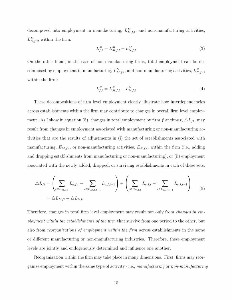
decomposed into employment in manufacturing, LMM,f,t, and non-manufacturing activities,

LMN,f,t, within the firm:

LMf,t = LMM,f,t + LMN,f,t (3)

On the other hand, in the case of non-manufacturing firms, total employment can be de-

composed by employment in manufacturing, LNM,f,t, and non-manufacturing activities, LNN,f,t,

within the firm:

LNf,t = LNM,f,t + LNN,f,t (4)

These decompositions of firm level employment clearly illustrate how interdependencies

across establishments within the firm may contribute to changes in overall firm level employ-

ment. As I show in equation (5), changes in total employment by firm f at time t,4Lft, may

result from changes in employment associated with manufacturing or non-manufacturing ac-

tivities that are the results of adjustments in (i) the set of establishments associated with

manufacturing, EM,f,t, or non-manufacturing activities, EN,f,t, within the firm (i.e., adding

and dropping establishments from manufacturing or non-manufacturing), or (ii) employment

associated with the newly added, dropped, or surviving establishments in each of these sets:

4Lft =

∑e∈EM,f,t

Le,f,t −∑

e∈EM,f,t−1

Le,f,t−1

+

∑e∈EN,f,t

Le,f,t −∑

e∈EN,f,t−1

Le,f,t−1

= 4LMft +4LNft

(5)

Therefore, changes in total firm level employment may result not only from changes in em-

ployment within the establishments of the firm that survive from one period to the other, but

also from reorganizations of employment within the firm across establishments in the same

or different manufacturing or non-manufacturing industries. Therefore, these employment

levels are jointly and endogenously determined and influence one another.

Reorganization within the firm may take place in many dimensions. First, firms may reor-

ganize employment within the same type of activity - i.e., manufacturing or non-manufacturing

15

activity. In this case, firms may fire employees in manufacturing establishments or close down

establishments, and hire new employees in other existing or newly opened manufacturing es-

tablishments. As a result of this reorganization, overall employment in the manufacturing

activity of the firm may decline, stay the same, or increase, depending on the number of jobs

eliminated relative to the number of jobs created. To illustrate this, Figure 1 shows how the

structure of the firm in my example changed from one period to the next as the firm closed

the establishment in manufacturing industry 1, kept the establishment in manufacturing

industry 2, and opened up a new establishment in manufacturing industry 5. The relative

importance of the changes in employment that resulted from these changes in the firm’s orga-

nizational structure determines the overall changes in manufacturing employment within the

firm. Similar types of reorganization within the non-manufacturing activity of the firm may

lead to similar changes in employment in non-manufacturing activities within firms. Second,

firms may reorganize employment across manufacturing and non-manufacturing activities.30

Firms may eliminate jobs in manufacturing activities by reducing employment within or

closing manufacturing establishments, and hire more employees in existing or newly opened

establishments in non-manufacturing activities such that overall firm level employment may

expand, shrink, or stay the same.31

Depending on the importance of the reorganization margin relative to the within- estab-

lishment adjustment, firms may expand in total employment or may expand in employment

associated with manufacturing or non-manufacturing activities. These may not be the same

jobs or the same employees in the same establishment of the firm classified to the same

industry, but the firm may expand in its overall activity or in a certain type of activity even

if it reduces employment in certain establishments. Thus, this suggests that within-firm re-

organization could reconcile the fact that companies that had manufacturing activities grew

30Bernard et al. (2016) documents that this type of reallocation is substantial in Danish firms.31For example, Apple’s publicly available yearly reports show that in the last two decades, the company

went through important organizational changes that mainly consisted of outsourcing all assembly to Foxconnin China, specializing in the production of high-tech sophisticated components in the US, and expandingdesign, engineering, R&D, and retail in the US.

16

over time, despite the fact that US manufacturing overall had been declining.

The possibility of within-firm reorganization may have implications for our understanding

and measurement of the impact of industry-specific shocks on domestic economic activity.

Since firms may reorganize from more exposed to less exposed industries, they may respond

differently in terms of employment to industry-specific shocks than establishments. This is

mainly because shocks with a differential impact across industries have differential impacts

across the establishments of the firms classified to different industries. Thus, the firm may

reduce employment in a negatively exposed industry by firing workers in or closing estab-

lishments classified to the exposed industries, while simultaneously expanding employment

in existing or newly opened establishments in less exposed or non-exposed industries.32 The

overall firm level impact of the shock will depend on the extent to which the new jobs created

within the firm through reorganization compensate for the decline in within firm employment

in exposed industries.

To illustrate this, I assume that manufacturing industry 3 in Figure 1 is exposed to an

industry-specific shock. Thus, this firm may reduce employmen or close the establishment in

manufacturing industry 3, but expand or keep constant the level of employment in manufac-

turing industry 4 and non-manufacturing industry 1. At the same time, the firm may find it

profitable to enter new industries, such as manufacturing industry 5, or non-manufacturing

industry 2. An entry into manufacturing industry 5 would result in an expansion in the num-

ber of jobs in manufacturing within the firm; this could compensate for the decline in jobs

due to the exit of manufacturing industry 1. All of these could lead to a decline, increase, or

no change in manufacturing employment within the firm, depending on whether the newly

created manufacturing jobs compensate or not for the number of jobs eliminated by the

32This implies that in the two-stage least squares estimator of the effect of the shock on establishments, β, isan inconsistent estimator of the true effect, β. Let’s denote the change in employment within establishmentsover time by Y, the shock to a particular establishment by X and the instrument of the shock by Z. Ifreorganization is present, then in the two-stage least square estimator β = (Z ′X)−1Z ′Y = β + (Z ′X)−1Z ′εthe term (Z ′X)−1Z ′ε is not zero. This is because the presence of reorganization across the establishmentsowned by the same firm leads to a correlation between the shock and error term across the establishmentsowned by the same firm. Statistically, this leads to a block diagonal Z ′ε.

17

firm in manufacturing industry 1. This example clearly demonstrates that reorganization

as a margin of adjustment in firm level employment in response to industry-specific shocks

may allow firms to become net job creators even in manufacturing, despite the fact certain

manufacturing establishments shrink.

Using these definitions, in the next section I derive a decomposition of aggregate US

employment by firm and within-firm activity type. I use this decomposition to examine the

importance of reorganization within US firms and its implications for understanding aggre-

gate trends in US manufacturing employment. Then, as an example of an industry-specific

shock in the US, I consider the swift increase in imports from China to US manufacturing

industries that resulted from China’s entry into the WTO. I estimate the impact of this shock

on US manufacturing firms to show that reorganization within more exposed US firms was

so substantial that it allowed them to escape the negative impact of the shock and expand

employment in less exposed manufacturing industries.

1.3 Descriptive Evidence on Reorganization of US Firms

1.3.1 Data Sources

To characterize trends in employment by US manufacturing firms, estimate the causal im-

pact of the China shock on these firms’ employment, and document facts on the underlying

mechanism, this paper builds on a novel data set with firm-establishment-product as unit

of observation that covers the universe of US firms for Census years 1997, 2002, 2007, and

2012.33 I construct this data set by combining four micro databases from the US Cen-

sus Bureau: the Commodity Flow Survey (CFS), the Census of Manufactures (CMF), the

Longitudinal Business Database (LBD), and the Longitudinal Foreign Trade Transaction

33The industrial classification in the US changed from the Standard Industrial Classification to the NorthAmerican Industrial Classification System in 1997. In order to ensure my results are not contaminated bychanges in industrial classification, I stick to the sample period between 1997 and 2012 that allows me touse a consistent industrial classification over time.

18

Database (LFTTD).34 I use the resulting data set to extract four types of information.

First, I characterize firm level employment and the organization of employment by in-

dustries within these firms. I exploit a unique feature of the LBD that allows me to observe

the universe of firms in the US and their organizational structure across industries in terms

of number of establishments, number of employees, and payroll by SIC-4 and NAICS-6 in-

dustries. Each of the firms in the LBD has a unique firm identifier,35 and the dataset lists all

the establishments the firm owns. By using this information, I can characterize the mapping

between establishments and firms in the data. I measure the number of establishments and

firm level employment by counting the number of establishments of the firm and summing

employment across all establishments within the firm.

Each of the establishments of the firm is classified to an industry based on the main activ-

ity of the establishment. I use this information to define manufacturing activity (i.e., estab-

lishments with NAICS-2 between 31 and 33) and non-manufacturing activity (i.e., establish-

ments with NAICS-2 as 11, 21-23, and 42-81) within the firm. Next, I define manufacturing

and non-manufacturing employment, payroll, and the number of establishments within the

firm as the sum of employment and payroll across establishments, and the number of estab-

lishments associated with each kind of activity within the firm. I further define the number

of employees, payroll, and the number of establishments in retail-wholesale, transportation,

professional services, finance, information, etc. as the sum of employment and payroll across

the establishments classified to each of these industries36 within the firm. Next, using this

information, I define the firm’s type as manufacturing if the firm has non-zero employment

in manufacturing in t− 1.37 Finally, I define the firm’s main manufacturing industry as the

34The Data Appendix contains technical details on the particular features of these databases. Also, Iprovide details on the way these four datasets are merged at the firm-product and firm-establishment-productlevel.

35The Census Bureau creates these firm identifiers by using information from the Business Register startingfrom 2002, and Standard Statistical Establishment List prior to 2002.

36Table 2 in the Data Appendix provides the exact definition of these activities in terms of NAICS2classification.

37This definition of the manufacturing firm implies that the t− 1 is different for each t− 1, t pairs. Forinstance, t− 1 is 1997 when the 1997, 2007 years pair is considered.

19

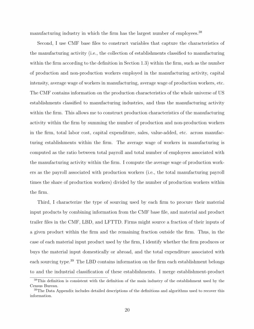
manufacturing industry in which the firm has the largest number of employees.38

Second, I use CMF base files to construct variables that capture the characteristics of

the manufacturing activity (i.e., the collection of establishments classified to manufacturing

within the firm according to the definition in Section 1.3) within the firm, such as the number

of production and non-production workers employed in the manufacturing activity, capital

intensity, average wage of workers in manufacturing, average wage of production workers, etc.

The CMF contains information on the production characteristics of the whole universe of US

establishments classified to manufacturing industries, and thus the manufacturing activity

within the firm. This allows me to construct production characteristics of the manufacturing

activity within the firm by summing the number of production and non-production workers

in the firm, total labor cost, capital expenditure, sales, value-added, etc. across manufac-

turing establishments within the firm. The average wage of workers in manufacturing is

computed as the ratio between total payroll and total number of employees associated with

the manufacturing activity within the firm. I compute the average wage of production work-

ers as the payroll associated with production workers (i.e., the total manufacturing payroll

times the share of production workers) divided by the number of production workers within

the firm.

Third, I characterize the type of sourcing used by each firm to procure their material

input products by combining information from the CMF base file, and material and product

trailer files in the CMF, LBD, and LFTTD. Firms might source a fraction of their inputs of

a given product within the firm and the remaining fraction outside the firm. Thus, in the

case of each material input product used by the firm, I identify whether the firm produces or

buys the material input domestically or abroad, and the total expenditure associated with

each sourcing type.39 The LBD contains information on the firm each establishment belongs

to and the industrial classification of these establishments. I merge establishment-product

38This definition is consistent with the definition of the main industry of the establishment used by theCensus Bureau.

39The Data Appendix includes detailed descriptions of the definitions and algorithms used to recover thisinformation.

20

level information from the CMF to firm-establishment mapping in the LBD. The resulting

data set contains information on firms, the establishments of these firms, and the output and

material input products of each firm’s establishments. Thus, it becomes possible to identify

whether a given material product used by the firm as material input is produced within the

firm or procured from a third-party supplier. I assume that a given product of the firm

results from domestic in-house production if there are two establishments within the firm

such that one of them produces the product (i.e., the product is in the set of outputs of the

establishment), while the other establishment uses the product as material input (i.e., the

product is in the set of material input products of the establishment). Thus, this product

is both output and material input within the firm. Once I have retrieved this information,

I aggregate from the firm-establishment-product level to the firm-product level to measure

the value and quantity of product at the firm level that is sourced from internal production

of the firm (“domestic insourcing” hereafter).

The LFTTD import file contains information on the value and quantity of products,

defined at the HS-10 level, that the firm imported in a given year from a given country. The

LFTTD also has information on whether the import transaction is between related parties40

or is an arm’s-length transaction. Thus, I can distinguish between foreign direct investment

(i.e., FDI) and foreign outsourcing. Using this information I identify, in the case of each

HS product, if it falls into the category of foreign insourcing (i.e., produced in a plant of

the firm located abroad) or foreign outsourcing (i.e., procured from a third-party supplier

located abroad). Moreover, in the case of each firm-product pair, I define the value and

quantity of imports from the five major trading partners of the US (i.e. Canada, China,

Germany, Japan, and Mexico)41 by using information about the country of origin of each

40Section 402(e) of the Tariff Act of 1930 defines related-party trade as transactions between partieswith relationships as directly or indirectly, owning, controlling, or holding poIr to vote 6 percent or moreof the outstanding voting stock or shares of any organization. Other sources of the US Census Bureaureport that “a related party transaction is one between a U.S. exporter and a foreign consignee, whereeither party owns (directly or indirectly) 10 percent or more of the other party”. For more information, seehttps://www.census.gov/foreign-trade/Press-Release/edb/2009/techdoc.pdf.

41These five countries together account for about 70% of the international trade transactions of the USwith the rest of the world.

21

import transaction.

To get a consistent product classification across products in the CMF, identified by

NAICS-6 codes, and the products in the LFTTD, identified by HS-10 codes, I use the

concordance tables constructed by Pierce and Schott (2011). This allows me to merge each

HS-10 product code in the LFTTD import file with its NAICS-6 counterpart in the CMF.

Then, I collapse the LFTTD import files from the HS-10 to the NAICS-6 product levels

by adding up total value and quantity across the HS-10 products imported by the firm

that fall into the same NAICS-6 category. Similarly, to measure total expenditure on foreign

insourcing and outsourcing by NAICS-6 product category, I aggregate from HS-10 to NAICS-

6 the total value and quantity of products imported based on arm’s length and related party

trade transactions.

I merge the firm-product level information, resulted from combining the LBD and CMF

files, to the firm-product level information, which resulted from collapsing the import files

to the firm-product level. The resulting data set contains information on the set of products

used by the firm as material inputs; the value and quantity used by domestic insourcing,

foreign insourcing, and foreign outsourcing; and the value and quantity of imports by the

five major trading partners of the US. I assume that a material input product of the firm

is sourced from a domestic supplier (“domestic outsourcing” hereafter) if the expenditure

on the product by the firm is not zero after I subtract from the total per-product material

expenditure the value of imports and the value of domestic in-house production.

Fourth, I construct material input and output prices at the NAICS-6 product level by

using the material and product trailer files from the CMF. These files contain information

on the set of products used by the establishments of the manufacturing firm as material

inputs, and the set of products produced by the establishments of the manufacturing firm as

outputs. These files also record values and quantities of each of these products by NAICS-6

digit. I define prices as unit values computed as the ratio between the value and quantity.42

42Unit value as a proxy for prices is widely used in the international trade and industrial organizationliterature when prices are not directly observed. For instance, Amiti and Konings (2007) use this definition

22

Finally, I augment the microdata described in this section with publicly available in-

formation on US manufacturing industries. More precisely, I use information from the UN

Comtrade Database to construct the measures of the China shock to US manufacturing in-

dustries and their instruments. In particular, I use information on exports from China to

the US and exports from China to the rest of the world at the six-digit HS product level. I

use the concordances created by Pierce and Schott (2011) between HS, SIC-4, and NAICS-6

industrial classifications to quantify imports from China to US manufacturing industries de-

fined at the four-digit SIC level.43 In addition, I use the NBER-CES Manufacturing Industry

Database for 1997 and 2007 to measure the value of shipments, the price index associated

with these shipments with base year in 2007, and the employment of US manufacturing

industries, defined as the collection of establishments classified to the same four-digit SIC

manufacturing industry.

1.3.2 Trends in US Firms’ Employment and Organization

To show that reorganization has implications for trends in employment, in this section I

derive a decomposition of aggregate US employment. In particular, I decompose the growth

rate of aggregate employment into growth due to manufacturing and non-manufacturing

firms, and manufacturing and non-manufacturing activities within these firms. I apply the

decomposition to the data described in the previous section. The decompositions indicate

that reorganization across industries was substantial, particularly in the case of US manufac-

turing firms, and led to a different trend in firm level employment relative to trends observed

at the establishment level.

Consistent with the findings of previous literature, aggregate US employment in estab-

lishments classified to manufacturing industries declined between 1997 and 2012. However,

to define the prices of Indonesian plants, and DeLoecker et al. (2016) define in this way the prices of Indianplants. The main caveat of the material input and output product trailer files is that in some cases, firmsdo not report quantities. The US Census Bureau has attempted to impute the missing quantities. However,these imputed quantities lead to outliers in the unit values. Thus, I only use the information on prices whenquantities are reported by the firm. For more detail, see White et al. (2012) and White (2014).

43The Data Appendix discusses these datasets in detail.

23

firms that owned declining US manufacturing establishments not only eliminated jobs in

manufacutring by firing workers from manufacturing plants or closing plants, but also cre-

ated jobs by hiring more workers in non-manufacturing industries such as retail-wholesale,

professional services information, administrative support, and management. These findings

suggest that if we look at trends in aggregate employment in the US through the lens of

the firm instead of the establishment, the aggregate employment picture looks better: Reor-

ganization within firms across industries allows firms to compensate for employment losses

created in manufacturing. These may not be the same workers or the same jobs in the same

industries, but firms that manufactured created jobs in net.44 In what follows, I derive the

decomposition and discuss the results.

Given the definition of the types of firms and activities within these firms in Section 1.3,

I derive a decomposition of aggregate national level employment, Lt, by firm and activity

types within the firm. Aggregate national employment at each time t can be decomposed as

the sum of employment across manufacturing and non-manufacutring firms:

Lt =∑

f∈FM,t

LMf,t +∑f∈FN,t

LNf,t = LMt + LNt (6)

By using the definition of the manufacturing and non-manufacturing activities within the

firm, this can further be decomposed into employment in the two types of activities within

the firm:

Lt =∑

f∈FM,t

LMM,f,t +∑

f∈FM,t

LMN,f,t +∑f∈FN,t

LNM,f,t +∑f∈FN,t

LNN,f,t (7)

= LMM,t + LMN,t + LNM,t + LNN,t

where the first two terms of the sum are aggregate employment in manufacturing, LMM,t, and

non-manufacturing, LMN,t, activities by manufacturing firms, while the last two terms are

44There still could be important distributional effects of trade on workers with different types of skills orworkers located in regions that were more affected by the China shock.

24

aggregate employment in manufacturing, LNM,t, and non-manufacturing activities, LNM,t, by

non-manufacturing firms.

Given the decomposition of aggregate employment in (7), the growth in aggregate na-

tional employment between time t− 1 and t, ∆Lt/Lt−1, can be decomposed into four com-

ponents: (i) adjustment due to change in employment in manufacturing, ∆LMM,t/Lt−1, and

(ii) non-manufacturing, ∆LMN,t/Lt−1, activities of manufacturing firms, and (iii) adjustment

due to changes in employment in manufacturing, ∆LNM,t/Lt−1, and (iv) non-manufacturing,

∆LNN,t/Lt−1, activities of non-manufacturing firms:

∆LtLt−1

=∆LMM,t

Lt−1

+∆LMN,tLt−1

+∆LNM,t

Lt−1

+∆LNN,tLt−1

(8)

I apply the decomposition in (8) to the data described in the previous section. First, I use

the sample of surviving firms. The results of the decomposition on the sample of surviving

firms are striking. As Table 1 indicates, manufacturing firms in the US contributed by 4

percentage points to the 28 percentage points expansion in aggregate employment between

1997 and 2007. This net job creation by firms that owned the manufacturing establishments

in 1997 was possible, as the number of jobs they created in non-manufacturing industries (i.e.,

a 7 percentage points increase in the number of jobs in non-manufacturing activities relative

to total employment in 1997) fully compensated for the number of jobs they eliminated in

manufacturing industries between 1997 and 2007 (i.e., a 3 percentage points decline in the

number of jobs in manufacturing activities relative to total employment in 1997). Thus, this

descriptive fact clearly shows that firms’ reorganization across industries was substantial and

it had implications for trends in their employment.

To identify the type of the activities that led to the expansion of employment in non-

manufacturing industries by surviving manufacturing firms, I further decompose the growth

of aggregate employment in the non-manufacturing activities of manufacturing firms by

25

NAICS-2 industries.45 This decomposition is based on the following accounting equation:

∆LMN,tLMN,t

=

∑n∈N ∆LMn,tLMN,t

(9)

where n ∈ N is defined as the non-manufacturing activity mapped into the data at NAICS-2

levels such as retail-wholesale, transportation, information, administrative services, manage-

ment, professional services, health, education, etc. Table 2 shows the results of the decom-

position. Activities such as management, administrative services, information, and retail-

wholesale expanded substantially, and became an important part of the non-manufacturing

activities of US manufacturing firms. Thus, hiring more people in management, logistics,

and technology jobs allowed firms that were initially engaged in manufacturing to grow, and

compensate in aggregate for the number of jobs they had eliminated in manufacturing.

These decomposition results are robust to other measures of the size of the firm’s activ-

ities, such as the number of establishments or payroll. Figure 2 shows that manufacturing

firms went through important organizational changes as they opened more establishments

in non-manufacturing industries than the number of establishments they had closed in man-

ufacturing industries. Moreover, the findings are also robust to other time periods than

the one considered in the baseline analysis. In particular, Figures 2 and 3 show that US

manufacturing firms went through important organizational changes not only over the 1997

and 2007 period, but also over the 1997-2012 period. Similarly, Figure 4 demonstrates that

the findings are robust even if I allow for switching in and out of manufacturing by defining

the manufacturing firm as a firm that has non-zero employment in manufacturing in any

of the census years between 1997 and 2012. The decomposition results are also robust to

alternative definitions of the manufacturing firm. In Table 3, I show the results of the de-

composition based on equation (8) by defining the firm that manufactured in 1997 as the

firm that had a ratio of employees in manufacturing activities relative to the total number

45Table 22 of the Data Appendix gives the list of these activities and the NAICS2 codes associated withthem.

26

of employees greater than 5 percent.46 The results of the decomposition are very similar to

the ones obtained based on the baseline definition of the manufacturing firm.

Finally, I use the sample of all the firms and apply this to the decomposition derived

in equation (8). As the results of the decomposition reported in Table 4 show, accounting

for firm entry and exit does not change the main conclusion of the baseline analysis: US

manufacturing firms went through important cross-industry reorganization over time as they

created jobs in non-manufacturing that compensated for the number of jobs they had elim-

inated in manufacturing. This reorganization had implications for the trend in aggregate

employment.

The facts outlined in this section strongly suggest that firms have an additional margin

to adjust employment relative to establishments: reorganization across industries. Thus,

firms may respond to industry-specific shocks by not only adjusting employment within

the establishments they own, but also by dropping and adding establishments in the same

or different industries in which they were present when the shock hit them. Intuitively,

this reorganization may allow firms to escape the negative impact of unfavorable shocks

in certain industries by expanding their activity in less exposed or non-exposed industries.

Thus, taking into account the reorganization margin by moving the unit of analysis from the

establishment to the firm may have implications for our understanding and measurement of

the impact of industry-specific shocks on US manufacturing employment. The next section

considers the swift increase in imports from China to US manufacturing industries, caused

by China’s entry into the WTO as an example of an industry-specific shock, and examines

its impact on US manufacturing firms.

46This definition of the manufacturing firm is used by Bernard et al. (2016) to document facts about thede-industrialization pattern that the Danish economy went through in the last decade.

27

1.4 The Impact of Chinese Imports on US Manufac-

turing Employment

In this section, I estimate the causal impact of the surge in Chinese imports in US output

markets - which resulted from China’s entry into the WTO in 2001 - on the employment

of US manufacturing firms. By using the manufacturing firm as the unit of analysis in-

stead of the manufacturing establishment, this analysis takes into account the possibility

of cross-industry reorganization within US firms. Estimation results indicate that more ex-

posed manufacturing firms in the US did not reduce employment; instead they expanded

employment in (i) manufacturing activities by hiring more production workers, whom they

paid higher wages, and (ii) services complementary to high-skill and high-tech manufactur-

ing, such as R&D, design, engineering, and headquarters services. These findings suggest

that within-firm reorganization allowed US firms to escape the negative impact of the China

shock by moving their activities to non-exposed industries, where they could grow.

China joined the WTO in 2001, which was followed by a large wave of non-tariff-based

trade liberalization between China and the rest of the world. Administrative, institutional,

and other non-tariff barriers on Chinese exports vanished (Chow, 2007; Kroeber, 2016). This

triggered a surge in Chinese imports in US manufacturing industries: Aggregate imports from

China to the US grew by 210.8 percent between 2001 and 2007 relative to the 1997 level,

whereas the growth rate was only 50.2 percent between 1997 and 2001.47 This rise in Chinese

imports varied widely across US manufacturing industries. The electrical equipment and

furniture industries registered the largest increase in Chinese imports, while food, beverages,

and textiles exhibited the smallest increase.48

The surge in Chinese imports created more competition in US manufacturing indus-

tries as imported Chinese goods competed with goods produced in the US. What did this

47For instance, Amiti and Freund (2010) documents the sectorial composition of this import growth.48The Appendix provides detailed information on the institutional background of China’s entry into the

WTO and its implications for the changing patterns of trade flows over time (i.e., imports and exports ofgoods) between China and the rest of the world, in aggregate and by industries over the 1997-2012 period.

28

increased import competition do to employment in US manufacturing firms? On the one

hand, the increased competition in US output markets may have caused US manufacturing

firms to reduce employment or even exit US output markets in which they could not compete

with Chinese imports (i.e., exposed industries). However, the possibility of reorganization

may have given these firms the opportunity to enter other US output markets in which

they had a competitive and comparative advantage relative to China (i.e., less exposed or

non-exposed industries). This reorganization within US manufacturing firms may have been

directed toward both manufacturing and non-manufacturing industries in the US. On the

other hand, the increased competition in US input markets may have incentivized US man-

ufacturing firms to increase employment in non-exposed US output industries in which they

were already present, or enter and expand employment in new ones in which they had a

comparative and competitive advantage relative to China. This is because increased compe-

tition in input markets induces a decline in the prices of material inputs, and thus a decline

in the cost of materials that firms use in the production of output. Therefore, the increased

Chinese import competition in US input markets may have acted as a favorable cost shock

to US manufacturing firms. This favorable shock may have compensated for or even over-

turned the negative impact of output market competition effect on US manufacturing firms’

employment. In other words, the combined effects of increased Chinese imports in US input

and output markets could have led to an expansion in US manufacturing firms’ employment,

even in manufacturing industries. Therefore, as Figure 1 illustrates, the overall impact of the

China shock on the employment of US manufacturing firms is ambiguous, as the adjustment

in firms’ employment through reorganization and the favorable cost shock caused by China

could have compensated for the decline or dampened the decline in more exposed industries.

By following the previous literature (Autor et al., 2013; Acemoglu et al., 2016; Bloom et

al., 2015; Hummels et al., 2016), I estimate the causal impact of increased Chinese imports

in US output markets (“China shock” hereafter) on the employment of US manufacturing

29

firms in two steps.49 First, I estimate the impact on US manufacturing industries. As the

data come in cross-sections, one way to account for firm entry and exit is to aggregate from

the firm to the industry level. In the second step, I estimate the impact on surviving US

manufacturing firms. The rest of this section outlines this analysis and presents the results.

1.4.1 The Impact on US Manufacturing Industries Defined Based

on the Firm

The methodology I use to measure the size and the impact of the China shock on employment

by US manufacturing industries builds on recent work by Acemoglu et al. (2016), and Autor

et al. (2013, 2015), Bloom et al. (2015) and Hummels et al. (2016).50 In particular, I use

the same identification strategy and the same measure of the China shock as these authors.

This consists of measuring the difference in changes in employment across initially similar US

manufacturing industries with different levels of exposure to the surge in Chinese imports.

However, in contrast to these papers, I take into account adjustments in employment due

to reorganization by moving the unit of analysis from the establishment to the firm, and

consequently from the industry as defined by establishment type - as in the aforementioned

papers - to the industry as defined by firm type.

There are two advantages of performing the analysis at this level of aggregation. First, the

industry-level analysis allows me to compare results with previous findings in the literature

that used industries defined based on the establishment as the unit of analysis (Acemoglu

et al., 2016). This comparison can be used to assess the importance of the reorganization

margin. Previous studies used the standard definition of the manufacturing industry, based

on which the US Census Bureau and BLS publish industry level data. According to this

definition, employment in a manufacturing industry i at time t, Lit, is defined as the sum

49This type of analysis is in line with the one used in Trefler (2004).50Future work will bring in the third way of measuring the shock. This is the PNTR tariff gap between

China and the US used by Pierce and Schott (2016).

30

of employment across establishments classified to manufacturing industry i at time t based

on the largest activity within the establishment: Lit =∑

e∈MEiLe,t, where ME

it is the set of

establishments in the US that have their largest activity in manufacturing industry i in year

t. However, this definition of the manufacturing industry ignores the firm and, thus, the fact

that decisions across establishments within the firm are interdependent, and reorganization

across industries is possible. An alternative definition of the manufacturing industry takes

into account the firm, and potential interdependencies between establishments owned by the

same firm and, thus, allows for adjustment in employment due to reorganization. According

to this definition, employment in manufacturing industry i at time t, Lit, is the sum of

the employment across firms classified as manufacturing industry i at time t based on the

largest manufacturing activity within the firm,51 Lit =∑

f∈MFitLf,t, where MF

it is the set

of US manufacturing firms that have their largest manufacturing activity in manufacturing

industry i at time t. The main advantage of this definition relative to the standard one is

that it keeps the organizational structure of the firm together in the same unit of observation

(i.e., manufacturing industry in this case). Moreover, it allows me to quantify employment

associated with manufacturing, LM,i,t =∑

f∈MFitLM,f,t, and non-manufacturing activities,

LN,f,t =∑

f∈MFitLN,f,t, within the manufacturing firm as Lit = LM,i,t + LN,f,t. Thus, any

difference in estimates obtained based on the standard versus the alternative definitions of the

manufacturing industry is suggestive evidence of how the reorganization margin contributes

to the estimated causal impact of the China shock. The second advantage of the industry-

level analysis is that it allows me to take into account entry and exit, which ensures that

selection is not driving the estimation results.

I estimate the impact of increased Chinese imports on industry-level employment by

using the identification strategy used by Acemoglu et al. (2016), Autor et al. (2013, 2015),

Bloom et al. (2015) and Hummels et al. (2016). This consists of estimating the following

51In line with the BLS and US Census Bureau definitions of the main economic activity, industry i is themanufacturing industry with the largest number of employees within the firm.

31

regression model:

4logYit = β0 + β1Shockit + β2Xi1997 + εit (10)

where4logYit is the log change in employment in manufacturing industry i from 1997 to 2007

defined in the alternative ways, 4logLit. As industries with a larger increase in imports from

China may also be exposed to other shocks that drive employment down over time, I control

for industry characteristics in the pre-shock year. These controls ensure that identification

of the causal impact of the China shock is based on comparing two industries that would

have shown the same trend in employment over time had the China shock not differentially

impacted them. Thus, Xi1997 contains a set of industry-level controls defined in 1997, which

can be grouped in two categories:52 (i) two-digit industry fixed effects that account for

differential trends in employment across two-digit manufacturing industries and allow me to

identify the impact of the China shock from variation in the shock variable across industries

within the same two-digit industry,53 and (ii) a series of other industry level controls defined

in the base year, 1997, which allow for identification by using variation in the shock variable

across industries with relatively similar technological characteristics. In line with the existing

literature, I include in this category control variables such as capital intensity (defined as

the ratio between capital expenditure and total employment); share of production workers

(defined as the ratio between the number of production workers and total employment) as a

proxy for skill intensity of the industry; share of payroll and employment in manufacturing

activities (defined as the ratios between the payroll in manufacturing activities and total

payroll, and as the ratio between the number of employees in manufacturing activities and

52Following the previous literature, the third category of industry level controls would include variablesthat control for pre-trends in industry level employment. As employment in manufacturing has been decliningfor the last three decades, it could be the case that by focusing only on the period between 1997 and 2007,the estimated impact overstates the impact of the China shock on US industry level employment. Themicrodata used in this paper does not allow me to construct industry level employment earlier than 1997, asthe first year observed is 1997. However, as Acemoglu et al. (2016) show, controlling for the pre-trend doesnot have a significant impact on the estimates of the causal impact of increased imports on employment byindustries defined based on establishment type.

53For instance, this allows me to compare plastic and chemicals industries, or machinery manufacturingand electrical equipment rather than a broader comparison such as textile versus electrical equipment.

32

total employment).54

Shockit measures the change in exposure to Chinese imports in manufacturing industry

i between 1997 and 2007. β1 captures the impact of the China shock on industry level

employment, as it measures how changes in employment differ across initially similar US

manufacturing industries that were differentially exposed to the China shock. I define the

Shockit variable in two ways, by closely following Acemoglu et al. (2016), Autor et al. (2013,

2015), Bloom et al. (2015) and Hummels et al. (2016). To ensure the comparability of my

results with those of previous literature, I define the industry at the four-digit SIC level as

in previous papers.

The first measure I use to quantify the China shock to US manufacturing industries is the

growth rate of imports from China to US manufacturing industries, defined as the change in

log Chinese imports between 1997 and 2007:

∆logMCH,USit = logMCH,US

i,2007 − logMCH,USi,1997 (11)

where MCH,USi,t is defined as the value of imports from China to the US in manufacturing

industry i, defined at the four-digit SIC industry level, in year t and in 2007 dollars. This

measure of the China shock is the industry level version of the measure used by Hummels et

al. (2016) to quantify the impact of increased imports on Danish firms and their employees’

wages55 and is consistent with the industry level measure used by Bloom et al. (2015).

The year 1997 represents the pre-shock year, while 2007 the post-shock year. I choose

1997 as the base year, since it is the earliest year for which I have access to microdata. Also,

1997 is four years before China liberalized its international trade by joining the WTO and,

thus, it was still uncertain in 1997 when China would actually join WTO. As a consequence

54Acemoglu et al. (2016), Autor et al. (2013), and Pierce and Schott (2016) argue that, by controlling forthese industry characteristics, one can ensure that the estimated impact is not contaminated by shocks dueto technological progress.

55Hummels et al. (2016) aim to estimate the causal impact of increase in total imports by Danish firmson their employees’ wages. This paper focuses on imports from China, which constitute a certain fraction oftotal imports.

33

of this liberalization, Chinese firms could freely enter international markets, export profitably

based on their comparative advantage of having access to cheap, low-skilled labor (Paulson,

2015; Naughton, 2007), and upgrade productivity, all of which further increased Chinese

exports (Hsieh and Ossa, 2016).56 Thus, the measure in (11) intends to capture the change

in Chinese imports in US manufacturing industries driven by the Chinese export supply

shock.

To isolate the variation in measure (11) due to supply shocks in China, I instrument it by

using the growth rate of imports from China to the eight major trading partners of China:

∆logMCH,OTHit = logMCH,OTH

i,2007 − logMCH,OTHi,1997 (12)

where MCH,OTHi,t is defined as the value of imports from China to the eight major trading

partners of China, except the US, in manufacturing industry i in year t, evaluated in 2007

dollars. The identification assumption is that the eight major trading partners of China were

similarly exposed to the Chinese supply shock as the US, and import demand shocks were

correlated across these high-income countries.57 This identification strategy is in line with

Acemoglu et al. (2016), Autor et al. (2013, 2014), Bloom et al. (2015) and Hummels et al.

(2016). Table 4 contains descriptive statistics for the measures in (11) and (12), and reveals

a large variation in the growth of Chinese imports across US manufacturing industries. The

large R2 and t-statistics indicate a strong predictive power of the instrument for the shock in

Table 5, suggesting that industries in other developing countries that registered significant

56Appendix provides more details on the institutional background of this liberalization.57This identification strategy is only valid if the only driving forces behind the surge in Chinese exports

to the rest of the world between 1997 and 2007 were shocks that originated from China and not shocks thatoriginated in the rest of the world (i.e., any type of shock that drove up demand for Chinese exports). Inthis respect, these identification assumptions are somehow in the spirit of the Hausman (1996) instrumentfrequently used in the industrial organization literature (i.e., instrument the price by the prices of the sameproduct by the same firm in other markets). Based on a comparative advantage argument, industries thatregister a decline in demand for US production are the industries in the other countries that register a largeincrease in demand for Chinese imports. This negative correlation in demand shocks biases the two stageleast square estimates downward and, thus, leads to underestimation of the true effect. As I expect thatreorganization allows firms to expand employment in response to increasing imports from China, the trueeffect is even larger than the ones I estimate if demand shocks are correlated.

34

growth in Chinese imports were also the most exposed industries in the US.

The second measure of the Chinese trade shock is in line with Acemoglu et al. (2016)

and Autor et al. (2015). This measure is the change in the Chinese import penetration ratio

to US manufacturing industries over the period between 1997 and 2007 defined as:

∆IPRCH,USit =

∆MCH,USit

Yi,1997 +Mi,1997 −Xi,1997

(13)

where ∆MCH,USit is the change in real imports from China to US in manufacturing industry

i, defined as four-digit SIC, over the period 1997 to 2007. Yi,1997 +Mi,1997−Xi,1997 is the size

of the market in manufacturing industry i in the base year 1997, measured as the real value

of shipments, Yi,1997, plus the real value of net imports in industry i defined as the difference

between total imports, Mi,1997, and exports, Xi,1997.58

To isolate this variation in the change in the import penetration ratio in (13) from the

variation induced by potential demand shocks in the US that may have affected US demand

for Chinese imports, I use the identification strategy proposed by Acemoglu et al. (2016)

and related papers by Autor et al. (2013, 2015). Thus, I instrument (11) with the change

in the import penetration ratio from China to the eight major trading partners of China,

except the US, defined as:59

58All variables used to compute the import penetration ratio are expressed in 2007 dollars. As industrylevel price indices for imports and exports are not available in the US, following Acemoglu et al. (2016), Iinflate imports from China to the US, total imports, and total exports in 1997 to prices in 2007 by using thePersonal Consumption Expenditure (PCE) index in 1997 with base year 2007. Moreover, I inflate the totalvalue of shipments by using the manufacturing shipment price index in 1997 with base year 2007, along withthe nominal value of shipments, in the NBER-CES database. More details on my choice of the deflator andits implications for estimating the impact of the increase in Chinese import competition on US manufacturingindustries defined based on aggregating from the establishments are included in the Appendix. The resultsof this exercise reported in the Appendix indicate that the choice of the price index to deflate US shipmentsmatters for the robustness of the estimated impact on industries aggregated from the establishments. Thus,depending on the type of the deflator used and the type of the shock measure applied, the estimates indicatethat the surge in Chinese imports had a negative or no effect on US manufacturing establishments.

59As a robustness check, I define another version of the instrument in which the change in imports fromChina to other countries is normalized by the lagged value of US market size (i.e., the value in 1994). Onemay worry that industries in the US in 1997 had already anticipated that China would join the WTO in 2001,and thus industry level employment was exposed to the anticipated trade shock. Thus, going back threemore years and using the lagged market value in the instrument would mitigate this potential simultaneitybias.

35

∆IPRCH,OTHit =

∆MCH,OTHit

Yi,1997 +Mi,1997 −Xi,1997

(14)

where ∆MCH,OTHit is the change in real imports from China to the eight major trading

partners of China, except the US, in manufacturing industry i between 1997 and 2007.60

Yi,1997 + Mi,1997 − Xi,1997 is defined as described in the case of measure (11). The identifi-

cation assumption is that the eight major trading partners of China were similarly exposed

to the Chinese supply shock as the US, but import demand shocks are not correlated across

these high-income countries.61 The descriptive statistics of the measures in (13) and (14)

reported in Table 4 demonstrate a large variation in changes in the Chinese import penetra-

tion ratio across US manufacturing industries. However, in comparison with the statistical

properties of the previous measure of the China shock, the growth rate of industry level

Chinese imports, this measure exhibits a large dispersion across industries. This suggests

that normalization in the import penetration ratio may induce more dispersion in the China

shock than dispersion in actual Chinese import growth across industries. Thus, we could

expect less precise estimates by using this measure of the China shock. Motivated by this,

I use the measure in (11) as the main measure of the exposure to Chinese imports. Then, I

use the second measure in the robustness check of my main results.62

Given these measures of the China shock and the identification assumptions, I estimate

the regression model in (10) by two-stage least squares. I weight all the regression estimates

by employment in 1997, which is the start of my sample period and the pre-China shock year.

I cluster the standard errors at the two-digit industry level, which allows for correlation in

60Following Acemoglu et al. (2015) and Autor et al. (2013, 2015), these countries are Australia, Denmark,Finland, Germany, Japan, New Zealand, Spain, and Switzerland.

61This identification strategy is only valid if the only driving forces behind the surge in Chinese exportsto the rest of the world between 1997 and 2007 were shocks that originated from China and not shocks thatoriginated in the rest of the world (i.e., any type of shock that drove up demand for Chinese exports). Inthis respect, these identification assumptions are very much in the spirit of the Hausman (1996) instrumentfrequently used in the industrial organization literature (i.e., instrument the price by the prices of the sameproduct by the same firm in other markets).

62The highly statistically significant point estimate of the coefficient on the instrument in the first-stageregression and the large R2 in Table 5 indicate that industries in other developed countries that registereda large increase in import penetration ratio from China also registered a large increase in the US.

36

errors across industries within a given two-digit industry category.63 Thus, the causal impact

of the China shock on US manufacturing industries is measured by two-stage least square

estimates of coefficient β1in model (10). The two-stage least square estimates are presented

in Tables 5 to 7. The robustness checks based on measure (13) are reported in the Appendix.

The estimation results can be summarized in three main findings. First, increased imports

from China did not lead to a decline in the employment of more exposed US manufacturing

industries. Estimates indicate that employment in more exposed US manufacturing indus-

tries relative to less exposed industries did not fall between 1997 and 2007. The estimation

results presented in Columns 2 of Table 5 suggest that when we aggregate from the firm to the

industry level, more exposed industries expanded employment relative to the employment in

less exposed industries. The estimates imply a 1.5 percent yearly increase in employment of

the manufacturing industry with 75th percentile exposure relative to one with 25th percentile

exposure. This suggests that cross-industry reorganization may allow firms to escape the

negative impact of industry-specific shocks and expand employment. This finding is robust

to other measures of manufacturing industry size: More exposed industries expand in the

number of establishments, total payroll, and hours worked relative to less exposed industries

(Columns 3 and 4 of Table 5).

Second, estimation results indicate that expansion in overall employment of the more

exposed US manufacturing industries relative to less exposed ones is due to expansion of

employment in both manufacturing and non-manufacturing activities within these indus-

tries (Columns 5 and 6 of Table 5). By defining the industry based on the firm, the growth

rate of total industry level employment can be decomposed into changes due to adjustment in

employment in different activities within the industry. Thus, the impact of the China shock

on each of these components can be estimated to assess their contribution to the effect on

overall employment. Results reported in Table 6 indicate that manufacturing industries more

exposed to the China shock expanded employment of manufacturing activities, and head-

63The Appendix contains robustness checks by presenting estimation results with standard errors clusteredat the four-digit industry level.

37

quarter and professional services, while employment of retail-wholesale and transportation

activities did not change in response to the China shock. The estimates imply a 1 percent,

and 0.5 percent yearly growth in the number of manufacturing workers, respectively high-

skilled service workers in the manufacturing industry with 75th percentile exposure relative

to one with 25th percentile exposure. Expansion in the employment of headquarters and

professional services activities in the more exposed manufacturing industries is suggestive of

reorganization within more exposed US manufacturing industries toward non-manufacturing

activities that are highly complementary to skill- and high-tech intensive manufacturing, such

as R&D, advertising, design, engineering, finance, etc. These striking findings suggest that

the possibility of changing the organization of the overall activity of the firm, both within

and across manufacturing and non-manufacturing industries, may allow for growth of US

employment in industries in which the US has a comparative and competitive advantage

relative to China.

Finally, estimation results demonstrate that the growing employment in manufacturing

activities of the more exposed manufacturing industries is due to the expansion of produc-

tion activity rather than non-production activity. The point estimates in Columns 2 and

3 of Table 7 show that manufacturing industries more exposed to the China shock grew as

the number of production workers increased in the more exposed industries. This finding

is robust to other definitions of the size of production activity within manufacturing indus-

tries, such as the number of manufacturing establishments or the number of hours worked.

More exposed US manufacturing industries increased the number of manufacturing estab-

lishments in the US relative to the less exposed ones, while workers in these more exposed

US manufacturing industries worked more hours.

These findings are complementary to previous literature that uses the establishment as

the unit of analysis. For instance, relative to the findings of Acemoglu et al. (2016) or

Autor et al. (2013), my findings suggest that reorganization toward non-exposed industries,

in which the US has a comparative advantage relative to China, allowed US firms to create

38

jobs that more than offset the losses measured at the establishment level. These findings may

seem striking, but they are actually in line with the conclusions of Amiti and Wei (2006).64

They show that increased offshoring may have led to the expansion in employment of US

manufacturing industries, as cross-industry reallocation allowed for more efficient allocation

of resources in the domestic economy. However, the estimated impact of the China shock

on US manufacturing industries is a combination of within-firm and cross-firm adjustments

in employment in more exposed industries relative to less exposed ones. To assess the

importance of within-firm adjustment, the next part of the analysis focuses on estimating

the causal impact of the China shock on US manufacturing firms’ employment.

1.4.2 Impact on US Manufacturing Firms

The estimated impact of the China shock on the employment of US manufacturing industries

is a combination of within-firm impact and the reallocation of employment across firms

classified as the same industry. However, I also aim to understand the implications of

within-firm cross-industry reorganization for the measured impact of the China shock on US

manufacturing employment. Thus, this section quantifies the within-firm effect by estimating

the impact of increased imports in US output markets on the growth in employment of US

manufacturing firms between 1997 and 2007. This analysis allows me to assess to what extent

the industry level estimates are driven by changes in employment within firms relative to

the adjustment in employment across firms within more exposed manufacturing industries.

I estimate the impact of the China shock on the growth of overall employment and em-

ployment in different activities of US manufacturing firms by using an identification strategy

that is in line with the methodology I used in the industry level analysis in the previous

64They document that at a more aggregated industry level, three-digit NAICS, employment in US indus-tries that registered larger service ofshoring went up between 1992 and 2000.

39

section. This consists of estimating the following regression model:

4YftLf,1997

= β0 + β1Shockft + β2Xf,1997 + εit (15)

where 4Yft/Lf,1997 is the growth in overall employment of firm f from 1997 to 2007, and

the growth in employment by activities of the firm relative to total firm level employment

in 1997, Lf,1997.65 Xi1997 contains a set of firm level controls in 1997 that can be grouped

in two categories. The first is a set of four-digit industry fixed effects, defined based on the

main manufacturing industry of the firm in 1997;66 These account for differential trends in

employment across firms in different four-digit manufacturing industries. Thus, I identify

the impact of variation across firms within the same four-digit industry. The second is a

series of other firm level controls defined in the base year, 1997, that allow for identification

by using the variation in the shock variable across firms with relatively similar technolog-

ical characteristics. This category of control variables contains the capital intensity of the

firm, defined as the ratio between capital expenditure and total employment; the share of

production workers within the firm defined as the ratio between the number of production

workers and total employment, as a proxy for the skill intensity of the firm; the share of

payroll and employment in manufacturing activities within the firm, defined as the ratio

between the payroll in manufacturing activities and total payroll, and the ratio between the

number of employees in manufacturing activities and total employment. Shockft measures

the change in the firm’s exposure to increased Chinese imports through US output industries

in which the firm had a presence in 1997. Thus, β1 captures how changes in employment

differ across initially similar firms that have different levels of exposure to the China shock

due to differences in their initial pattern of industrial specialization.

65I measure the left-hand side variable as the change in each component of overall employment relative tototal firm level employment in 1997 instead of the change in log employment in order to account for zerosin the data. For instance, the firm can have positive employment in a particular activity in 1997 and zeroin another year.

66Following the alternative definition of the manufacturing industry outlined in Section 1.4.1., the mainmanufacturing industry in 1997 is the manufacturing industry within the firm with the largest number ofemployees in 1997.

40

I measure the China shock, Shockft,67 as the weighted average of the China shock to the

industries in which the firm had establishments in the pre-shock year, 1997. Thus, the firm

level measure of the China shock aims to take into account differences in the exposure to

the increase in Chinese imports across firms due to the differences in their initial pattern of

industrial specialization.68 As described in the previous section, the industry level shock is

defined in two ways: (1) the growth rate of Chinese imports in industry i, and (2) the change

in the Chinese import penetration ratio to industry i. Accordingly, the firm level shock can

be defined in two ways as the weighted average of these two industry level shocks.

The first measure of firm-level Chinese import shock is defined as the weighted average of

the growth in imports from China to the main output industry of the firm’s establishments

in the pre-shock year:

∆WMCH,USft =

∑e(i)∈If,1997

we(i),f,1997∆logMCH,USit (16)

where the weights, we(i),f,1997, are defined as described above and ∆logMCH,USit is measure

(11), as described in the previous section.

The second measure of firm-level Chinese import shock is defined as the weighted aver-

age of the change in import penetration ratios to the main output industries of the firm’s

establishments in the pre-shock year:

∆WIPRCH,USft =

∑e(i)∈Ef,1997

we(i),f,1997∆IPRCH,USit (17)

67The China shock to firms can be measured in two ways. A naive way would be to measure the shockto the main manufacturing industry of the firm by ignoring the fact that firms may do business in manydifferent manufacturing industries (i.e., most of the firms are multi-product). However, there may not onlybe important variation in this industrial specialization across firms that can be used to better identify theimpact of the China shock on firms, but there can also be correlation in the shock across industries withinthe firm.

68A similar idea is behind the China shock measure and the identification strategy used by Autor et al.(2013) to measure the impact of the surge in imports from China on local labor markets in the US. Theyexamine how changes in employment differ across US commuting zones that have different levels of exposureto Chinese import competition due to differences in their initial industrial specialization.

41

where we(i),f,1997 is the employment weight of establishment e of firm f classified to output

industry i, e(i), in the pre-shock year 1997, defined as the number of employees in establish-

ment e of the firm relative to the total number of employees of firm f in 1997, with Ef,1997

being the set of establishments that firm f has in 1997.69 ∆IPRUSit is the shock to industry

i defined by measure (13), as described in the previous section. Thus, cross-firm variation in

this shock measure comes from differences in the patterns of industrial specialization across

firms in 1997, and through this from variation in the shock across industries.

There are two advantages of measuring the shock to the firm in this way. First, this

measure takes into account differences in the pattern of industrial specialization across firms

as another source of variation, in addition to cross-industry variation in the shock. The

firm may have establishments in different industries that are exposed to the Chinese import

shock in different ways. By computing the weighted average of the industry specific shocks

within the firm, I take into account variation in the pattern of industrial specialization

across firms. Moreover, from a statistical point of view, the weighted average ensures that

I attribute greater importance to those industries in which the firm had larger economic

activity. Second, by computing the weighted average of the industry level shocks the firm

is exposed to, I account for potential within-firm cross-industry correlations in the China

shock.

Since the within-firm establishment employment weights are fixed to the pre-shock year,

the identification challenge I face at the firm level is similar to those in the industry level

analysis. To isolate variation in the firm-level measure due to supply shocks in China, I use

the industry-level instruments defined and described in the previous section, and bring it to

the firm level by using within-firm employment weights.70 Thus, I define the instrument to

69More precisely, the weights are constructed as follows: we(i),f,1997 =

Le(i),f,1997/(∑

e(i)∈Ef,1997Le(i),f,1997

)where Le(i),f,1997 is total employment by establishment e, classi-

fied to industry i, of firm f in 1997.70The identification assumption is that given the firms’ initial industrial specialization pattern, variation

in Chinese trade exposure through these industries is due to supply shocks that originate from China, asthe eight major trading partners of China are similarly exposed to the Chinese supply shock as the US.Moreover, the import demand shocks are not correlated across these high-income economies.

42

measure (17) as:

∆WMCH,OTHft =

∑e(i)∈If,1997

we(i),f,1997∆logMCH,OTHit (18)

Consistent with this, the instrument to measure (17) is defined as:

∆WIPRCH,OTHft =

∑e(i)∈Ef,1997

we(i),f,1997∆IPRCH,OTHit (19)

where ∆logMCH,OTHit and ∆IPRCH,OTH

it are the changes in the growth rate of Chinese im-

ports and Chinese import penetration ratio to developed countries other than the US, defined

as described in the previous section. The large R2 and t-statistics in Column 1 of Table 8,

and the ones in Table 28 in the Appendix, show a strong predictive power of the instruments

for the shocks. Moreover, the large values of the F-statistics confirm that these are relevant

instruments for the two measures of the firm level shocks.

Given firm-level measures of the China shock and the identification assumptions, I esti-

mate the regression model in (15) using a two-stage least squares method. Since the data are

in the form of cross-sections in each Census year, this allows for the estimation of the speci-

fication in (15) only on the sample of continuing firms. Thus, in this section, I conduct my

analysis on the sample of surviving US manufacturing firms. I weight all regression estimates

by firm level employment in 1997, which is the start of my sample period and the pre-China

shock year. I cluster standard errors at the four-digit industry level, which allows correlation

in errors across industries. Thus, the causal impact of the China shock on employment by

US manufacturing firms is measured by the two-stage least squares estimates of coefficient

β1 in model (15). In line with the industry-level analysis, I report the results based on the

first measure while I use the change in import penetration ratio as a robustness check.

Estimation results of the firm level analysis - summarized in Tables 8, 9 and 10 - yield

three sets of findings. First, more exposed US manufacturing firms did not reduce employ-

43

ment (Column 2 Table 8). The point estimate is positive, which suggests that more exposed

firms may have grown in total employment relative to less exposed firms. However, the co-

efficients are not statistically significant, as standard errors of the point estimates are large.

These are in line with the findings of Antras, Fort, and Tintelnot (2016), who document

a small and not statistically significant coefficient on growth in Chinese firm level imports

when they regress changes in surviving US firms’ overall employment on changes in the firms’

Chinese imports.

Second, more exposed firms expanded employment in manufacturing and reduced em-

ployment in non-manufacturing (Columns 3 and 4 of Table 8). Firms more exposed to

increasing Chinese imports in their output markets added jobs in headquarter and profes-

sional services (Columns 2 and 3 of Table 9). However, the China shock did not seem to

have a statistically significant impact on employment in retail-wholesale activities within US

manufacturing firms (Column 1 of Table 9). As the shock is measured to the set of the firm’s

industries in 1997, all of these represent suggestive evidence of within-firm reorganization

from exposed industries to less or non-exposed industries. As a result of this reorganization,

they may have expanded employment in manufacturing by hiring more workers in existing

or newly opened non-exposed manufacturing establishments, which fully compensated for

the number of workers they fired from the exposed establishments. Moreover, these find-

ings also suggest that the nature of reorganization toward non-manufacturing industries is

such that US firms that used to engage in manufacturing before the China shock expanded

in non-manufacturing industries that are complementary to high-skill, high-tech intensive

manufacturing such as management, financial planning, R&D, engineering, design, adver-

tising, etc. These findings are in line with those of the industry level analysis, suggesting

that the estimated industry level impact on manufacturing employment is mostly driven by

within-firm cross-industry reorganization, rather than cross-firm within-industry adjustment

in manufacturing employment in response to the China shock.

Finally, the within-firm expansion in manufacturing employment was the result of growth

44

in the number of production workers whom firms paid higher wages. More exposed US

manufacturing firms hired more workers in production activities, while they did not adjust

the number of non-production workers (Columns 1 and 2 in Table 10). Moreover, more

exposed firms spent on average more on workers in manufacturing activities, and in particular

on production workers, relative to less exposed firms. The point estimates reported in

Columns 3 and 4 of Table 10 indicate that more exposed firms registered an increase in

the average wage of production and manufacturing workers.71 The expansion in the scale

of manufacturing production was not only in terms of hiring more production workers in

manufacturing, but also by opening new plants (Column 5 of Table 10) and adding new

products to the set of output produced by the firm (Column 6 of Table 10).

All of these findings are suggestive of reorganization within manufacturing toward more

skill intensive industries, and are in line with the theoretical predictions of Burnstein and

Vogel (2016). They show that trade liberalization induces an increase in the skill premium

in countries with a comparative advantage in more skill-intensive sectors, as factors are

reallocated toward more productive and skill-intensive firms within sectors and toward skill-

intensive sectors.

As firms may be multi-product, an expansion in manufacturing employment may also

suggest that US manufacturing firms repositioned in the product space in response to the

China shock by dropping products from their product set that were cheaper to source from

China and adding new products in markets in which they could compete with the Chinese.

The data suggest that US manufacturing firms also went through this type of reorganization

too. In particular, they re-organized their production toward higher quality varieties within

the broadly defined output product groups. One of the best features of the data collected by

the US Census Bureau is that they provide information on the set of output products, values

at the factory gate and the quantities of each of these produced in the firm’s manufacturing

establishments at the six-digit NAICS level. Using this information, I define the real value

71This finding is in line with the increasing importer wage premium documented by Koren and Csillag(2016) in the case of Hungarian workers.

45

of output prices, priceoutputfept , in the US as the ratio between the value and quantity, adjusted

by industry level inflation between 1997 and 2007. Using this information on output prices, I

examine how US manufacturing firms adjusted the price of their output products in response

to increased Chinese imports. Thus, I estimate the following regression model on the sample

of firm-establishment-product pairs that survived between 1997 and 2007:72

4log(priceoutputfept

)= γ0 + γ1Shockpt + γe + εfept (20)

where 4log(priceoutputfept

)is the change in the price of output product p produced in estab-

lishment e owned by firm f at time t, γe contains a set of industry fixed effects that are

defined based on the main output industry of the establishment and controls for macroeco-

nomic shocks to the output prices that are common across firms in a given output industry.

Shockpt is the import penetration ratio from China to manufacturing industry p in the US,

as defined in Section 1.4.1. I use the same identification strategy and instrument the shock

variable by using the same instrument as outlined in Section 1.4.1. Thus, γ1 captures the

impact of the China shock on output prices in the US as the difference in the output price

between initially similar firm-establishment-product pairs in the same broadly defined out-

put industry, but with different exposure to Chinese import competition. The estimation

results reported in Table 23 in the Appendix are notable. They indicate that US firms that

manufactured output products in industries more exposed to Chinese import competition

registered an increase in the price of the output product they continued to produce in the

US. This is suggestive evidence of upgrading production in the US to higher quality output

varieties within the six-digit product category (Khandelwal, 2010; Amiti and Khandelwal,

2013; Medina, 2016) or an adverse effect of reorganization on prices (Conconi, Legros and

Newman, 2012; Legros and Newman, 2013).

All of these findings are suggestive evidence of reorganization of manufacturing activity

72Figure 9 in the Appendix shows the distribution of output prices in 1997 and 2007 in the case of thesample of surviving firm-establishment-product pairs, and indicates no significant shift in overall distributionof output prices over time.

46

within US manufacturing firms toward more skill-intensive manufacturing industries. This is

consistent with the predictions of the trade-in-tasks model of Grossman and Rossi-Hansberg

(2008),73 who show that trade liberalization, which resulted from reductions in the cost of

offshoring, may lead to expansion in domestic employment of less-exposed industries and an

increase in wages of the less exposed skill category. One way to capture this cross-industry

reorganization in a reduced-form way is to view the data through the lens of a firm that

may span multiple industries. As skill-intensive manufacturing industries are less exposed

or non-exposed to the China shock in the US, my findings are suggestive evidence of reor-

ganization within US manufacturing firms toward more skill-intensive manufacturing. This

cross-industry reorganization within US manufacutring firms may explain why firm level

manufacturing employment responds differently to the China shock than does establishment

level manufacturing employment, and may also reconcile my findings with those of previ-

ous literature, in which employment in more exposed manufacturing establishments declines

(Pierce and Schott, 2016). What is the potential mechanism that explains growth in em-

ployment within firms in non-exposed industries, toward which US manufacturing firms may

reorganize in response to the China shock? The next section describes a potential mechanism

through the lens of a theory of the firm and establishments, in which I imbed the Grossman

and Rossi-Hansberg (2008) offshoring task technology, and thus rationalizes the finding that

increased imports from China lead to reorganization and growth of skilled employment in

less exposed industries.

1.5 Theoretical Explanation

This section develops a theory of the firm and establishments in which I imbed the Grossman

and Rossi-Hansberg (2008) offshoring task technology. In this model, firms in the domestic

economy produce differentiated varieties by using two intermediate goods, each of which they

assemble using a continuum of tasks performed by high- or low-skilled workers. Assembly

73Any trade model that assumes relative factor endowment or productivity differences across countriespredicts that trade liberalization implies specialization based on comparative advantage. See Burnstein andVogel (2011) for a general framework.

47

of one of these intermediate goods is more skill-intensive than assembly of the other. Tasks

performed by low-skilled workers can be conducted in either the domestic economy or abroad,

where low-skilled labor is cheaper, but offshoring the task involves a cost that is heterogenous

across firms.

This framework rationalizes my main empirical finding, that US manufacturing firms

expanded manufacturing employment in response to the China shock through the following

mechanism. As a consequence of the decline in the cost of offshoring, firms re-organize their

domestic production; they shift their domestic activity into areas that are more skill-intensive

by offshoring tasks that are less skill-intensive. As the cost of offshoring exhibits heterogene-

ity across firms, a decline in the cost of offshoring has a differential impact on within-firm

cross-industry reorganization, the unit cost of production, and employment across firms.

Firms that register a larger decline in the cost of offshoring (i.e., more exposed firms) shift

more of the low-skill intensive tasks abroad and, thus, register a larger decline in the relative

cost of assembly of the intermediate goods. As a consequence, the price of the variety pro-

duced by the more exposed firm declines more relative to the price of the variety produced

by the less exposed firm. Thus, consumers substitute their consumption toward the variety

that registered the larger price decline. To meet the increasing demand, the more exposed

firm increases employment. If the two intermediate goods are complements in the production

of the final good variety, the more exposed firm expands employment of high-skilled labor

relative to less exposed firms by hiring more of these workers in the production of high-

skill-intensive intermediate good assembly (i.e., less exposed establishment within the firm)

relative to the number of high-skilled hired in the production of a low-skill-intensive inter-

mediate good (i.e., more exposed establishments within the firm). This section is organized

as follows. First, I present the assumptions and characterize the equilibrium conditions. I

then derive predictions on how a decline in the cost of offshoring impacts firms’ sourcing

decisions, costs of production, and employment.

48

1.5.1 Assumptions and Equilibrium Conditions

There are two countries: one domestic and one foreign. I assume that technologies are the

same in both. However, there is a productivity gap between the two countries. In particular,

I assume that the domestic country is more productive than the foreign country. Denoting

total factor productivities by A in the domestic country and A∗ in the foreign country, the

assumption on the productivity gap implies that A > A∗. This productivity gap generates

a gap in factor prices between the two countries, such that domestic wages are large relative

to foreign wages.

Domestic firms produce differentiated varieties. The production of variety z by any firm

f requires two intermediate inputs, j ∈ x, y.74 There are two labor skill types - low-skill,

L, and high-skill, H - used by the firm as factors of production to assemble intermediate

goods x and y. Production of a unit of either input x or y involves a continuum of low-skill

intensive tasks (L-tasks), and a continuum of high-skill intensive tasks (H-tasks). Firms

can either produce L-tasks at home or offshore them to the foreign country. The difference

in factor prices across countries incentivizes domestic firms to offshore (i.e., the benefit of

offshoring). However, to offshore a task, the firm must pay not only the wages of the foreign

country, but also the cost of moving the task abroad (i.e., the cost of offshoring tasks), which

is firm specific.75 Figure 5 presents a chart that illustrates the structure of this production

process. Given the differences in factor prices across countries and the cost of offshoring,

the domestic country exports the final good varieties to the foreign country, in exchange

for importing L-tasks from the foreign country in equilibrium.76 In the rest of this section,

I characterize the demand for varieties, firms’ production and offshoring technology, firms’

cost minimization, and profit maximization problem.

74Making these types of assumptions on the structure of production is common in industrial organiza-tion, international trade, and international macro literatures that study the role of intermediate inputs infirms’ pricing and production decisions (Acemoglu and Guerrieri, 2008; Amiti, Itskhoki, and Konings, 2014;Helpman, Koren, and Szeidl, 2016; Blaum, Lelarge, and Peters, 2016).

75This idea was first developed by Grossman and Rossi-Hansberg (2002) in a two-sector open economymodel.

76 This balances trade between the two countries.

49

1.5.1.1. Assumptions on Preferences and Technologies

Consumer preferences and demand: In each country, consumers derive utility from

the consumption of F differentiated goods. Their utility takes the standard constant elas-

ticity of substitution form:

U =

[F∑f=1

zb−1b

f

] bb−1

(21)

where zf denotes the quantity of variety f , and the elasticity of substitution across varieties

is b. Consumers’ utility maximization problem yields the demand for variety f :

zf =Y

P 1−bp−bf (22)

where P =[∑F

f=1 p1−bf

] 11−b

is the aggregate price index of the differentiated goods and Y is

the total income. I assume that labor supply is prefectly inelastic, and Y/P 1−b is normalized

to 1.

Production technology: Firm f produces variety z in the domestic economy by a

constant elasticity of substitution technology, using as inputs intermediate goods x and y :

zf =[γx

ε−1ε

f + (1− γ) yε−1ε

f

] εε−1

(23)

where ε ∈ [0,∞) is the elasticity of substitution77 between the intermediate goods x and y

in the production of z, while γ ∈ (0, 1) is the share of intermediate good x in the production

of z. Firm f assembles intermediate good. j ∈ x, y by using Cobb-Douglas technologies

77ε < 1 implies that intermediates x and y are complements in the production of z, while ε > 1 impliessubstitution between the two intermediates.

50

that combine low-skill, L, and high-skill, H, labor as factors of production:78

xf = ALαxf,xH1−αxf,x (24)

yf = ALαyf,yH

1−αyf,y (25)

where αx and αy are the shares of low-skill labor in the assembly of x and y. I assume that

the assembly of x is relatively high-skill intensive, which implies the parameter restriction

αx < αy. Firm f pays wages w for one unit of low-skill labor in the domestic country, and

w∗ for one unit of low-skill labor in the foreign country. One unit of high-skill labor costs s

in the domestic country, and s∗ in the foreign country.79

Following Grossman and Rossi-Hansberg (2008), I assume that production of a unit of

good j involves a continuum of low-skill tasks (L-tasks) and a continuum of high-skill tasks

(H-tasks), with the measure of each of these types of tasks normalized to one, i ∈ [0, 1].80

Moreover, in line with Grossman and Rossi-Hansberg (2008), I assume that tasks using the

same type of skill require the same amount of labor of that particular skill type.81

Offshoring technology: Firm f can perform L-tasks, i ∈ [0, 1], either in the domestic

economy or offshore them to the foreign country. Offshoring is preferred because of the

benefit of offshoring: Low-skill labor is cheaper in the foreign country, given the assumption

on the technology gap between the domestic and the foreign countries. However, offshoring

is costly. Following Grossman and Rossi-Hansberg (2008), I assume that firm f performing

L-task i pays βγf t(i) as the cost of offshoring one unit of task i. β is a shift parameter

that captures the technological characteristics of offshoring common across firms. γf is an

idiosyncratic component of the offshoring cost that captures the technological characteristics

78One way to think about assembly of these intermediate goods within the firm is to view them as twoestablishments within the firm that specialize in the assembly of different components used by the firm inthe production of the final good.

79I assume that the final good sector is small relative to the overall size of the economy. Therefore, firmsin this sector do not affect wages. This means that firms take wages as given.

80Ossa and Chaney (2013) introduces the Grossman and Rossi-Hansberg (2008) type of tasks based pro-duction technology in the Krugman (1979), and assume that final good varieties are produced by performingsequentially a continuum of tasks. They framework, however, does not make the distinction between inter-mediate goods with different skill intensity.

81For example, if tasks i and i’ are performed by the same skill type, then the factor requirement forperforming i and i’ is such that the same amount of labor is required for each. This implies that Lf,j =∫ 1

0Lf,jdi and Hf,j =

∫ 1

0Hf,jdi.

51

of offshoring specific to firm f , such that firms with lower γf face a lower cost of offshoring.

t(i) allows for heterogeneity in the cost of offshoring across tasks i ∈ [0, 1]. I assume that

t(i) is a continuously differentiable function, and βγf t(i) >1 for all i. i ∈ [0, 1] are ordered

such that the costs of offshoring are non-decreasing ∂t(i)∂i

> 0. I assume that tasks in the

production of the two intermediate goods have the same offshorability. This implies that

offshoring costs are similar in the case of x and y: tx(i) = ty(i) = t(i). Therefore, if If is the

fraction of offshored tasks, the unit cost of low-skilled labor is w(1− If ) + w∗∫ If

0βγf t(i)di

1.5.1.2. Equilibrium Conditions

Offshoring decision: The tension between the benefits and costs of offshoring creates a

trade-off that firm f faces when deciding about the set of L-tasks offshored and performed in

the foreign country. Since domestic wages are large relative to foreign wages and offshoring

is costly, only the firms in the domestic country engage in offshoring, and pay βγf t(i)w∗ for

one unit of task offshored and performed abroad.82 As the firm offshores to take advantage of

the lower foreign wage - but at the same time pays the cost of offshoring - the marginal task

performed in the domestic economy by firm f , If , is pinned down at the task for which saving

on the labor cost of performing the task abroad relative to performing it in the domestic

economy exactly balances the cost of offshoring:83

w = βγf t(If )w∗ (26)

This condition is the same in the case of both intermediate goods x and y, given the assump-

tion on the equality of the offshoring cost, tx(i) = ty(i) = t(i). Thus, If is the equilibrium

marginal L-task such that all L-tasks with index i ∈ [0, If ] are performed by firm f abroad,

while all L-tasks with index i ∈ [If , 1] are performed in the domestic country. Given these

assumptions, the wage bill for low-skilled labor hired by firm f to perform the L-tasks in

82Thus, the cost of offshoring is in fact a wage premium paid by the firm on the foreign wage.83Notice that in order to have an interior solution, If > 0, one additional assumption is needed: w >

βt(0)w∗. This assumption is made by Grossman and Rossi-Hansberg (2008), and makes offshoring sometasks profitable.

52

the assembly of intermediate good j consists of the wage bill of low-skilled who perform the

set of i ∈ [If , 1] in the domestic economy and the wage bill of low-skilled who perform the

set of i ∈ [0, If ] abroad. Thus, using condition (26), the cost of one unit of low-skilled labor

becomes wΩ(If ), where Ω(If ) is the cost-saving that results from offshoring, and is given

by the following expression:84

Ω(If ) = 1− If +

∫ If0t(i)di

t(If )(27)

Cost minimization: Given the equilibrium set of offshored L-tasks, the cost associated

with one unit of low-skilled worker, wΩ(If ), and one unit of high-skilled worker, s, firm

f solves the following cost minimization problem to determine the number of high- and

low-skilled workers to hire for assembly of intermediate good j ∈ x, y:

minLf,j ,Hf,j

wΩ(If )Lf,j + sHf,j − cf,jAL

αjf,jH

1−αjf,j

(28)

which implies the following relative factor requirement in the assembly of j:

Hf,j

Lf,j=wΩ(If )

s

1− αjαj

(29)

Given Cobb-Douglas technology, the cost of assembly of intermediate good j, which is

the total costs of low-skill, wΩ(If ), and high-skill labor, s is:

cf,j =1

A(wΩ(If ))

αj s1−αj (30)

As Ω(If ) < 1 for any If > 0 given ∂t(i)∂i

> 0, offshoring reduces the total cost of low-skill

labor. Given the heterogeneity in the cost of offshoring across firms and the properties of

the offshoring technology t(i), offshoring reduces the total cost of low-skill labor more in the

84This expression is derived by substituting in w(1− If ) +w ∗∫ If0βγf t(i)di the expression of w* given by

(26).

53

case of firms with a lower firm specific component of the offshoring cost(γf < γf ′

), as these

firms shift a larger set of L-tasks abroad in equilibrium,(If > If ′

).

The cost minimization problem of firm f also implies the following demand for high- and

low-skilled labor per unit of production of intermediates x and y:

Lf,j =αjΩ(If )

A(wΩ(If ))

αj−1 s1−αj (31)

Hf,j =1− αjA

(wΩ(If ))αj s−αj (32)

By using these, we can define the total number of high-skilled workers hired by firm f in the

assembly of intermediate good x and y, as hf,x = Hf,xx and hf,y = Hf,yy, where x and y are

the quantities of intermediate j ∈ x, y assembled by the firm in equilibrium. Thus, the

total number of high-skilled workers by firm f is given by hf = hf,x + hf,y. We can similarly

define lf,x, lf,y and lf .

Profit maximization: Firms f = 1, .., F engage in monopolistic competition. Hence,

each firm f faces a downward sloping demand curve, but it takes the price index of the final

good varieties, P , wages, and the consumers’ expenditure as given. Given the cost of assem-

bly of intermediate good j, cf,j, and the inverse demand for variety z, pf =(

YP 1−b

)− 1b z− 1b

f

with b > 1,85 firm f solves the following profit maximization problem:

maxxf ,yf

Πf =

(Y

P 1−b

)− 1b [γx

ε−1ε

f + (1− γ) yε−1ε

f

] ε(b−1)b(ε−1)

− cf,xx− cf,yy (33)

The solution to this problem pins down the relative requirement of intermediate goods x and

y for the production of final good variety f as a function of relative unit costs:

y

x=

γ

1− γ

(cf,ycf,x

)−ε(34)

85The condition b > 1 guarantees the existence of the firm’s optimum. Otherwise, if b < 1 the markupover the marginal cost is negative and the firm does not find it profitable to produce.

54

1.5.2 The Impact of the Decline in the Cost of Offshoring on

Firms’ Sourcing Decisions and Employment

In this section, I consider how the decline in the cost of offshoring L-tasks impacts firms’

sourcing decisions, their cost of production of the final good, and their demand for skilled

labor in the domestic country.86 A decline in the cost of offshoring L-tasks in the model

is equivalent to a reduction in parameter β. This is equivalent to the China shock in my

empirical exercise. In the following propositions, I summarize the results of a comparative

statics analysis in the partial equilibrium.87 In particular, for given wages, I show how (i)

the marginal L-task, If , and thus the set of offshored L-tasks [0, If ]; (ii) the cost of sourcing

L-tasks, Ω(If ); and (iii) the total employment of high-skilled, and (iv) the employment of

high-skilled in the production of high-skill intensive intermediate good x, hf,x, relative to

the demand for high-skill in the production of low-skill intensive intermediate good y, hf,y,

change88 in the case of firm f in response to a decline in β. Moreover, I derive predictions

on how all these margins adjust in the case of a firm that is more exposed to a decline in β

(i.e., has a lower γf ) relative to a less exposed firm (i.e., has a larger γf ).

Proposition 1 If If > 0, then in equilibrium the set of L-tasks offshored by firm f

expands as β declines:

If > 0 (35)

Proof See the Appendix.

Proposition 1 shows that if offshoring L-tasks becomes cheaper as β declines, firms off-

shore more of the L-tasks abroad. These newly offshored tasks are performed by foreign

low-skill labor, while firm f performs more skill-intensive tasks in the domestic country.

This intuition is in line with Grossman and Rossi-Hansberg (2008).

Proposition 2 If If > 0, then in equilibrium the cost of sourcing L-tasks by firm f

declines as β declines:

Ωf < 0 (36)

86One can think of the domestic country as the US, and the foreign country as China.87In particular, I assume that the final good sector is small relative to the overall size of the economy.

Therefore, firms in this sector do not affect wages.88 Throughout this section, I measure the changes in log-differences and denote them with hat. For

instance, the change in variable If measured in log-difference, is If = dIf/If .

55

Proof See the Appendix.

Proposition 2 states that as the cost of offshoring L-tasks declines, firm f registers a

decline in the cost of assembly of intermediate goods. This is the combination of two effects.

First, holding the marginal task, If , constant, the decline in β leads to a decline in the

cost of production of firm f (i.e., direct cost effect of offshoring). Second, as summarized in

Proposition 1, the decline in β leads to a reorganization of the set of L-tasks across borders

(i.e., expansion in the set of L-tasks offshored), which further increases the cost saving from

offshoring (i.e., reorganization effect of offshoring). Thus, the second effect reinforces the

decline in the cost of production resulted from the first effect. Consequently, the overall cost

of assembly of both intermediate goods x and y falls. However, as y is the less skill-intensive

intermediate good, firm f registers a larger decline in the cost of assembly of y than in the

case of the more skill-intensive intermediate good x. In this way, the assembly of y is more

exposed to the decline in the cost of offshoring.89 This intuition is in line with Grossman

and Rossi-Hansberg (2008).

Proof See the Appendix.

Proposition 3 If If > 0, then the equilibrium employment of high-skilled by firm f

increases as β declines if and only if ε < b:

hf > 0 (37)

Proof See the Theory Appendix.

Proposition 3 shows that the decline in the cost of offshoring has an implication for high-

skilled labor employed by firm f . It states that the number of high-skilled hired by the firm

increases if the elasticity of substitution between the final good varieties (i.e., b) is larger than

the elasticity of substitution between the high- and low-skill intensive intermediate goods in

the production of the final good varieties (i.e., ε). The intuition behind this is the following.

89If we view the assembly of x and y within the firm as two establishments within the firm specialized inthe assembly of different components used by the firm in the production of the final good, then this resultimplies that the more exposed establishment registers a larger decline in the cost of production.

56

The decline in β leads to a decline in the cost of production as summarized by Proposition

2. As a result of this cost reduction, the variety produced by the firm becomes cheaper. As

varieties are substitutes in the consumption basket of the consumer (i.e., b > 1), the demand

for the variety of the firm increases. To meet the increasing demand, the firm expands the

scale of production of the final good variety (i.e. output expansion effect of offshoring) by

hiring more skilled-workers.90 However, as the decline in β leads to a larger decline in the cost

of assembly of y, the firm tends to substitute towards the cheaper input, y, which is less skill

intensive. This leads to an expansion of the low-skilled and a contraction of the high-skilled

employment at the firm level. Condition ε < b ensures that the output expansion effect is

large enough to trigger such a large expansion in the skilled-employment that it compensates

for the decline resulted from the substitution to the cheaper input. This intuition is in line

with the results of other papers that document theoretical results, in frameworks lacking the

firm, that cross-industry reorganization of the domestic economic activity in response to the

decline in the cost of offshoring (Grossman and Rossi-Hansberg, 2008), migration (Burnstein

et al., 2016) or capital deepening (Acemoglu and Guerrieri, 2008) can lead to an expansion

of the domestic economic activity.

This prediction of the model highlights the fact that even if certain tasks are offshored,

which may have negative consequences on the firm’s employment, other tasks are performed

at a larger scale in the domestic economy. Therefore, even if there is no reorganization, the

firm’s employment may increase, as reduction in the cost leads to an expansion in the scale

of production. Reorganization amplifies this effect, as it leads to further cost reduction and

ouput expansion.

Proposition 4 If If > 0, then, as β declines, the equilibrium employment of high-skilled

by firm f in the assembly of intermediate input x (i) increases relative to the equilibrium

employment of high-skilled in the assembly of intermediate input y if and only if ε < 1:

hx,f − hy,f > 0 (38)

90Thus, the condition on the elasticity of substitution between the final good varieties triggers the expansionin the output.

57

(ii) decreases relative to the equilibrium employment of high-skilled in the assembly of in-

termediate input y if and only if ε > 1:

hx,f − hy,f < 0 (39)

and (iii) there is no effect if ε = 1.

Proof See the Theory Appendix.

Proposition 4 shows that the decline in the cost of offshoring has an implication for high-

skilled labor hired in the less exposed establishment of the firm (i.e., the assembly of x, which

is more skill-intensive) relative to the more exposed establishment. It states that the number

of high-skilled hired in the assembly of x increases relative to the number of high-skilled hired

in the assembly of y if and only if x and y are complements in the production of the final

good variety f (i.e. ε < 1). The intuition behind this is the following. The decline in β leads

to a decline in the cost of production (Proposition 2). As a result of this cost reduction, the

price of the variety produced by the firm becomes cheaper which trigger an expansion in the

demand. To meet the increasing demand, the firm expands the scale of production of the

final good variety. If x and y are complements in the production of the final good variety

(i.e., ε < 1), then the firm expands the assembly of both x and y. This is associated with an

expansion of high-skill employment, such that the firm hires more of the high-skilled in the

assembly of the more skill-intensive intermediate x. However, x is less exposed to the decline

in β, since it employs fewer low-skilled. Therefore, the decline in the cost of offshoring leads

to a larger expansion of high-skill employment in the less exposed establishment of the firm

relative to the more exposed establishment.91

Proposition 5 If If > 0, If ′ > 0, γf < γf ′ , and∂2t(If )

∂I2f

< 0, then (i) the equilibrium set

of L-tasks offshored by firm f expands more relative to firm f ′ as β declines:

If > If ′ > 0 (40)

91The condition on the elasticity of substitution between intermediate goods in the production of the finalgood varieties (i.e. ε < 1) triggers the expansion of skilled employment in the less exposed establishmentrelative to the more exposed establishment.

58

(ii) in equilibrium the cost of sourcing L-tasks by firm f declines more relative to firm f ′ as

β declines:

Ωf ′ < Ωf ′ < 0 (41)

(iii) the equilibrium employment of high-skilled by firm f increases more relative to firm f ′

as β declines if and only if ε < b:

hf > hf ′ > 0 (42)

(iv) the relative equilibrium employment of high-skilled by firm f in the assembly of inter-

mediate input x increases more relative to firm f ′ as β declines if and only if ε < 1:

hx,f − hy,f > hx,f ′ − hy,f ′ > 0 (43)

Proposition 5 shows that the decline in the cost of offshoring has a heterogenous impact

across firms. Firms with a lower idiosyncratic component in the cost of offshoring L-tasks

(γf ) register a larger expansion in the set of offshored L-task and, thus, a larger cost decline if

the task specific component of the offshoring cost is concave (i.e.∂2t(If )

∂I2f

< 0). This condition

guarantees that the marginal cost of offshoring is decreasing in If . This means that firms

with a lower γf (i.e., firms that offshore more initially) can offshore an extra unit of L-tasks at

a lower cost and, thus, benefit more from the decline in β. As a consequence, they register a

larger expansion in the set of offshored L-tasks, a larger cost saving, and a larger expansion

in high-skilled employment relative to less exposed firms. Moreover, these more exposed

firms expand more the employment of high-skilled in the less exposed establishment relative

to the more exposed establishment.

The qualitative prediction summarized in part (iii) of Proposition 5 is consistent with

the findings documented in Section 1.4: increased offshoring to China led to an expansion

of high-skilled employment by US manufacutring firms. As part (iv) of Proposition 5 shows,

this expansion in high-skilled employment documented from the data may be the result of a

larger expansion of high-skilled employment in the non-exposed establishments of the firm.

As in the model the non-exposed establishments are in high-skilled intensive industries, in

which the home country has a comparative advantage, the model suggests the expansion of

59

high-skilled employment in response to the China shock documented from the data may have

been the result of US firms increasing high-skilled employment in non-exposed industries in

the US.

1.6 Empirical Evidence on the Proposed Mechanism

In this section I document a series of empirical facts that provide evidence of the mechanism

through which firms expand domestic high-skilled employment. The theory presented in

Section 1.5 predicts that the decline in the cost of offshoring of low-skill intensive intermediate

goods induces an expansion in the set of intermediates sourced from abroad by firms in the

domestic economy (Proposition 1). This reorganization of domestic economic activity allows

firms to register a decline in the cost of production (Proposition 2). As costs fall, the price of

the final good variety falls; this leads to an expansion in the demand. To meet the increasing

demand, firms expand the scale of domestic production of the final good by assembling more

intermediate goods. As more and less skill-intensive intermediate goods are complements in

the production of the final good variety, firms expand the scale of assembly. As a consequence

of this, firms expand high-skilled employment (Proposition 3) by hiring more of this skill

type in the less exposed establishment (i.e., more skill intensive intermediate good) relative

to the more exposed establishment within the firm (Proposition 4). Finally, the theory also

predicts a larger effect of the decline in the cost of offshoring in the case of the more exposed

firm relative to the less exposed (Proposition 5). The rest of this section provides suggestive

evidence for these theoretical predictions.92 In particular, I document how US manufacturing

firms changed their material input sourcing decisions over time. I then consider the change

in Chinese import competition in US input markets between 1997 and 2007 as a measure of

92Anecdotal evidence and publicly available reports of major manufacturers in the US provide informationthat is in line with the findings of this section. For instance, a senior board member of a major car manu-facturer declared, “we buy components from wherever is cheaper ... what we save on sourcing from abroadwe reinvest in the US to expand our business ... a typical carmaker hires more software engineers, computerscientists and electrical engineers than blue collar.”

60

the cost shock that resulted from China’s entry into the WTO, which hit US firms through

the markets in which they sourced their material inputs. I estimate the impact of this

cost shock on US firms’ sourcing decisions and material input prices (i.e., proxy for the

cost of sourcing material inputs) as a test of Proposition 1 and 2, and parts (i) and (ii) of

Proposition 5. Finally, I document how the rise in firms’ material input sourcing impacted

manufacturing employment by US manufacturing firms as a test of Proposition 3 and part

(iii) of Proposition 5.

1.6.1 Increased Offshoring to China

According to Proposition 1, the decline in the cost of offshoring low-skilled intensive tasks,

which in our case is China’s entry into the WTO, induces an expansion in the set of inter-

mediates sourced by firms from abroad. Part (i) of Proposition 5 predicts that this effect is

larger in the case of more exposed firms relative to the less exposed ones. To check whether

this prediction is in line with the data, I document how US manufacturing firms changed

their material input sourcing over time and estimate the causal impact of the China shock

on these firms’ sourcing decisions.

The richness of US microdata allows me to characterize and analyze changes over time in

firms’ material input sourcing decisions at the six-digit product level and across four types

of sourcing: buy or produce material inputs in the US or abroad. Thus, I decompose the

expenditure by firm f in year t on material input, p, by the country of origin of the sourcing

from the US (i.e., domestic) or a foreign country (i.e., imported):

MaterialfptMaterialfpt

=Domestic materialfpt

Materialfpt+Foreign materialfpt

Materialfpt(44)

Moreover, I decompose both the domestic and the foreign components based on whether

the material input is produced in a plant owned by the firm (i.e., insourcing) or procured from

61

a third-party supplier (i.e., outsourcing). Thus, each of the domestic and foreign components

of the material input expenditures can be decomposed by these two margins:

Domestic materialfptMaterialfpt

=Domestic Insourcingfpt

Materialfpt+DomesticOutsourcingfpt

Materialfpt(45)

Foreign materialfptMaterialfpt

=Foreign Insourcingfpt

Materialfpt+ForeignOutsourcingfpt

Materialfpt(46)

I apply the decompositions in (45)-(46) to a data set that I construct on US manufacutring

firms with firm-material input product as the unit of observation. The product is defined

at the six-digit NAICS level.93 This data set allows me to quantify each element of the

decomposition based on the definitions and assumptions outlined in Section 1.3. The results

of the decomposition are presented in Tables 11-13 in the form of weighted averages of

each component of the decomposition.94 These results provide a series of novel findings

that convey information on how US manufacturing firms organize their sourcing of material

inputs, as well as how these sourcing patterns have changed over time, in particular after

China’s entry into the WTO in 2001.

First, the results show that US manufacturing firms most frequently source the largest

share of their material inputs from independent suppliers, and in particular domestic sup-

pliers, rather than produce them in-house in the US or abroad. Table 11 shows that the

typical firm sources between 25 percent and 30 percent of its material inputs from in-house

93The data appendix provides a detailed description of how this data set was constructed.94To account for within-firm heterogeneity across product groups, and for the cross-firm heterogeneity in

the size of the material expenditure, I compute the weighted average of each component of the decompositionacross the material input product categories within the firm. I then compute the weighted average of thefirm level weighted averages across firms. The product weight within the firm is computed as the totalexpenditure on a particular material input product relative to the total firm level material expenditure. Thefirm level weights are computed as the firm level material input expenditure relative to the total materialexpenditure in the cross-section.

62

production95 as about 10 percent of the materials are produced in-house in the US96, while

material inputs produced in a factory owned by the firm abroad and shipped back to the

firm in the US for further processing account for about 15 percent or 20 percent of the total

material spending. In terms of foreign sourcing, Table 12 shows that a typical firm sources

most of its materials from the five major trading partners of the US (i.e., Canada, China,

Mexico, Germany, and Japan) such that most of the material sourcing from China involves

buying from Chinese suppliers rather than producing the input in China through foreign di-

rect investment.97 As Table 13 indicates, firms frequently mix different sourcing types (i.e.,

about four out of ten cases). In particular, they frequently both buy and produce inputs in

the same six-digit product category.98

Second, my findings on decomposition by industries suggest an important cross-industry

heterogeneity in the importance of each type of sourcing in firms’ sourcing strategy. As

Figures 6 and 7 indicate, industries that are less site specific or are more assembly intensive,

such as electrical equipment or transportation equipment, rely more on outsourcing, both

at the extensive (i.e., the frequency of choosing a particular sourcing type) and intensive

margins (i.e., the share of spending on a particular sourcing type). By comparing sourcing

95This number is larger than the one documented by Atalay et al. (2015), who decompose the totalmaterial spending of US firms by domestic in-sourcing and domestic out-sourcing (i.e., they only considerthe first component of the decomposition considered in this paper, based on equation 40). They find that USmanufacturing establishments in the US source about 9 percent of their materials from other establishmentsthat are vertically integrated within the firm. This number is about the same as the 10 percent that Idocument. However, if one takes into account the fact that firms in the US can own establishments in othercountries which may specialize in the production of the material inputs that the firm uses for the productionof its output in the US, then this number goes up to 25 percent as documented in Table 14. This suggeststhat once we take into account the fact that the boundary of the firm can expand across borders, firmsdo vertically integrate to source materials from in-house production and facilitate the shipment of thesematerials.

96This is not a surprising finding, as most of the shift from vertical integration toward outsourcing in theUS had occured by the early 1990s (Whitford, 2005).

97As Table 15 indicates, about 90 percent of the expenditure on sourcing from China in the case of atypical material input product of a typical US firm that manufactures in the US is based on arm’s-lengthtransactions rather than related-party trade transactions.

98This is suggestive evidence of the fact that risks related to contracting with independent suppliers, dis-ruption in supply chains, the presence of other types of transaction costs (Antras and Chor, 2013; Grossmanand Hart, 1986; Loertscher and Riordan, 2016; Williamson, 1985), or the presence of quality differentiationwithin the six-digit product category may induce the firm to produce some of the total required quantityof a particular input or some varieties of a particular input classified as the broad six-digit NAICS productcategory.

63

patterns across industries based on the country of foreign outsourcing, firms in industries

that are more assembly intensive by low-skill workers tend to source more from China (Tables

14 and 15). For instance, firms in the electrical equipment industry tend to source more of

their inputs from China than firms in the transportation equipment industry.

Third, by comparing distribution of material expenditure by the four types of sourcing

across years, Table 11 shows a rapid shift from domestic to foreign sources between 1997

and 2007. This mostly occured after 2001, when China joined the WTO. In addition to

this, Table 12 indicates that most of this shift took place in terms of switching to Chinese

suppliers rather than foreign direct investment in China. Moreover, this shift in sourcing

from domestic to Chinese suppliers is more pronounced in the case of firms in industries that

use material inputs that are more assembly intensive by low-skilled workers or are less site

specific, or where transporting in large volumes is not expensive (Table 14).

All of these descriptive findings suggest that, in line with the predictions of the theory,

China’s entry into the WTO shaped US firms’ sourcing strategies across borders and coun-

tries. This was particularly true in the case of firms in US manufacturing industries that

are intensive users of material inputs for which China has a comparative advantage. To

provide direct evidence of the causal impact of this link, I estimate the impact of increased

Chinese import competition in US input markets on US manufacturing firms’ input sourcing

decisions. In particular, I estimate a system of four equations, as follows:99

4yfpt = α0 + α1Shockpt +Xf,1997 + εfpt (47)

where 4yfpt is a vector with four components 4Domestic InsourcingfptMaterialfpt

, 4DomesticOutsourcingfptMaterialfpt

,

4Foreign InsourcingfptMaterialfpt

, and4ForeignOutsourcingfptMaterialfpt

. Each of these components capture the change

99As choices across the four types of sourcing of a particular material input product by the firm areinterdependent, changes in expenditures over time on the four types of sourcing are also interdependent.Thus, to capture this correlation when the impact of the China shock on the change in each componentof the decomposition is estimated, I set up the econometric model as a system. The other advantage ofestimating the system is related to the efficiency of the estimates, as correlation in errors across the fourequations of the system can be taken into account.

64

in the expenditure share by firm f and material input product p on a particular sourcing

type between 1997 and 2007.100 Shockpt captures the change in Chinese import competition

in the US manufacturing industry that firm f sources the material input from. I define

the China shock by using the two industry level measures presented in Section 1.5. Xf,1997

contains a series of firm level controls defined in the pre-shock year 1997, such as the main

manufacturing industry of the firm defined at the three-digit level and total employment of

the firm in manufacturing activities taken in logarithm. To assess the causal impact of the

China shock on firms’ sourcing strategy choice, I use the same identification strategy and

instrument as outlined in Section 1.4.

I find that US manufacturing firms that sourced their material inputs from industries that

were more exposed to the China shock tended to shift the sourcing of their material inputs

from domestic suppliers toward foreign sources (i.e., both foreign suppliers and by producing

the material input in factories owned by the firm abroad). In particular, estimates reported

in Table 17 indicate, using both definitions of the China shock, that US manufacturing firms

sourcing from industries more exposed to the China shock reallocated resources across the

four types of sourcing: they reduced spending on domestic suppliers, and increased offshoring

to the rest of the world.101 These more exposed industries in the US registered a large influx

of imports from China (i.e., the industries in which China had a comparative advantage).

Thus, this finding is empirical evidence of the theoretical prediction (Proposition 1, part (i)

of Proposition 5) that a decline in the cost of offshoring of low-skill intensive intermediate

goods induces a larger expansion in the set of intermediates sourced from abroad by more

exposed firms relative to less exposed.

100Given the form of the specification in (24), α1 captures the adjustment in the expenditure shares acrossthe four types of sourcing within a product category. Thus, it does not take into account product enty andexit, and the possibility that the China shock may have led to introduction of new imported varieties to theset of material inputs used by the firm (Broda and Weinstein, 2006; Goldberg, Khandelwal, Pavcnik, andTopalova, 2010).101This finding is in line with Antras et al. (2016) who show in a counterfactual exercise that China’s entry

to WTO increased offshoring of US firms not only to China but also to other countries.

65

1.6.2 Cheaper Material-Input Sourcing Due to China

As Proposition 2 and part (ii) of Proposition 5 summarize, the shift in sourcing toward

foreign locations must have been accompanied by a larger decline in the cost of materials

in the case of more exposed firm relative to the less exposed. To test this prediction in the

data, I examine how the unit cost of material inputs used by US manufacturing firms in the

production of their output adjusted in response to the China shock.

One of the unique features of the data on US manufacturing firms collected by the

Census Bureau is that it contains information on the set of material input products used

by the manufacturing establishments of the firm, and the value and the quantity associated

with these material inputs at the six-digit NAICS level of aggregation. I define the cost of

the material input, costinputfept , as the real unit value computed as the ratio between the value

and quantity and adjusted by industry level inflation between 1997 and 2007. To ensure

that outliers in the cost measure do not contaminate the results of the analysis, I remove

observations below and above the 5th and the 95th percentile when I construct the sample

for estimation.102 I plot in Figure 8 the distribution of these material input costs in 1997

and 2007 in the case of firm-establishment-product pairs that are present in both years. The

figure does not indicate any substantial shift in the distribution of these material input costs

to the right or left between 1997 and 2007, but it indicates an increase in the tailedness of

the distribution.103

To examine how these material input costs were adjusted between 1997 and 2007 in

response to increased Chinese import competition in US input markets, I write down and

estimate the following regression model both on the set of surviving firm-establishment-

102The choice of percentile size does not have any impact on estimation results, which are robust for othercleaning rules, such as dropping observations below and above the 3rd or 10th, and 97th and 90th percentiles.103The shape of the cost distribution in 2007 in comparison with the shape of the distribution in 1997

clearly shows that there is an increase in the mass of the costs greater than the median in 1997 and a declinein the mass of costs larger than the median, while the tails stay approximately unchanged over time.

66

product pairs and on the entire sample:104

4costinputfept = γ0 + γ1Shockpt + γe + εfept (48)

where γe contains establishment characteristics such as a set of industry fixed effects that

are defined based on the main output industry of the establishment and controls for macroe-

conomic shocks to material input costs that are common across firms in a given output

industry. Shockpt is defined in Section 1.4. I use the same identification strategy and in-

strument the shock variable by using the same instrument as outlined in Section 1.4. Thus,

γ1 captures the difference in material input costs across initially similar firm-establishment-

product pairs, but with different exposure to Chinese imports in the market of material input

p.

I find that US manufacturing firms that sourced material inputs from industries more

exposed to the China shock registered a decline in the cost of the material input in 2007

relative to 1997. Table 18 reports the two-stage least squares estimates of γ1 on the sample

of surviving (Columns 1 and 2) and on the sample of all firm-establishment-product pairs

(Column 3). These estimates indicate that an average 10 percentage point increase in imports

from China to the US induces an average decline in the firms’ cost of materials between 1

percent and 3.5 percent. This finding supports the theoretical prediction that the decline

in the cost of offshoring the production of low-skill intensive intermediates induces a decline

in the unit cost of production. There can be different channels through which this cost

reduction occurs, even if the model does not explicitly account for different sources of the

decline in the unit cost. For instance, the decline in upstream prices in the US due to

the pro-competitive effect of Chinese imports is one channel (Amiti and Konings, 2007;

104The entire set consists of the cross-sections in 1997, 2002, and 2007 pooled over time. Thus, it accounts fornot only the surviving firm-establishment-product pairs, but also for the firms, establishments, and productsthat entered or exited between these years. When I estimate the model on the set of all firm-establishment-product pairs, the estimated model in levels is: costinputfept = γ0 + γ1Shockpt + γf + γp + γe,t + εfept, where γfand γp control for variations in prices that are common over time in the case of a firm f and product p pair.γe contains establishment characteristics such as a set of industry fixed effects defined as the main outputindustry of the establishment.

67

Loecker, Goldberg, Khandelwal and Pavcnik, 2016; Feenstra and Weinstein, 2016); others are

access to new imported intermediate goods that are cheaper in China (Broda and Weinstein,

2006; Goldberg, Khandelwal, Pavcnik, and Topalova, 2010), and buying or producing the

intermediate good more cheaply in China.

1.6.3 The Role of Cheaper Sourcing in the Adjustment of US

Manufacturing Employment

The theory predicts that a decline in the cost of offshoring induces an increase in domestic

employment of high-skilled (Proposition 3, part (iii) of Proposition 5). This is possible,

since offshoring of low-skill intensive tasks allows domestic firms to reduce the cost of pro-

duction and, thus, expand the scale of production of the final good, for which they hire more

high-skilled labor. Thus, according to this theory, the decline in the cost of offshoring acts

as a favorable cost shock to the firm. In the previous sub-sections I documented empirical

evidence that the China shock was a favorable cost shock to US firms. This section ex-

amines whether the boost in US manufacturing firms’ material expenditure, resulted from

the favorable cost shock due to China, had a direct impact on these firms’ employment in

manufacturing activities. This consists of estimating the following regression model:

4LMftLf,1997

= β0 + β14logMaterialft + β2Xf,1997 + εit (49)

where 4LMft/Lf,1997 is the growth in manufacturing employment by firm f from 1997 to

2007,105 4logMaterialft is the change in the logarithm of real value of total material ex-

penditures of firm f from 1997 to 2007, Xi1997 contains a set of firm level controls in 1997,

which are the same as those listed in Section 1.4.2. To identify variation in material ex-

penditure over time due to the declining cost of sourcing induced by China, I instrument

105I measure the left hand side variable as the change in each component of employment by activity relativeto total firm level employment in 1997, instead of the change in log employment, to account for zeros in thedata.

68

4logMaterialft with the weighted average of the industry specific instrument defined in

Section 1.4.1.106 The weights are defined as the share of total spending on material input

p by firm f relative to the total material expenditure of the firm in 1997.107 Thus, the

two-stage least squares estimate of β1 measures the difference in manufacturing employment

across two firms that, on average, have the same initial characteristics in 1997, but one reg-

istered a larger increase in spending on materials than the other due to the larger exposure

to the change in Chinese imports by the US manufacturing industries that firm f sourced

its material inputs from (i.e., larger exposure to the favorable cost shock).

My findings indicate that US manufacturing firms that spent more on materials, by taking

advantage of the favorable cost shock due to China, expanded manufacturing employment

more. The highly statistically significant and positive point estimate of β1 in Column 2 of

Table 19 provides empirical evidence that US manufacturing firms expanded employment

in manufacturing industries less exposed to the China shock. This shock not only created

import competition in some of their output industries, but also reduced the cost of sourcing

their material inputs, which made possible the expansion of the scale of production and

employment of US manufacturing firms in industries in which the US had a comparative

advantage relative to China. Columns 3 to 5 provide additional reduced-form evidence of

US manufacturing firms expanding the scale of their domestic production in response to the

favorable cost shock due to China. In particular, more exposed firms hired more production

workers in manufacturing, opened more plants and added new products to the set of outputs

they produced.

Column 1 of Table 20 provides additional empirical evidence that supports this hypoth-

esis. This specification contains as right hand side variable, in addition to the ones listed

106The last two rows of Column 1 in Table 19 contain the value of the F-statistics and the associated p-valueof the F-test that tests, in the first-stage, the relevance of this instrument for the change in log materialexpenditure of the firms that manufactured in 1997. The zero p-value and the large value taken by theF-statistics indicate that this is a strong instrument.107More precisely, wp,f,1997=Materialp,f,1997/

∑p∈P input

f,1997Material,f1997. By using this weighting scheme, I

capture all the upstream shocks the firm is exposed to through the material input product it uses. Moreover,material input products that are less important in the production of the output product (i.e., low cost share)are given less importance through the small weight in the computation of the instrument.

69

above: the firm level China shock measure from Section 1.4.2 that is actually the measure of

the China shock to which the firm is exposed in its output markets (i.e., weighted average of

the China shock to the output industries the firm has establishments in). The sign and size

of the point estimates suggest that the mechanism through which China induced expansion

in the manufacturing employment of US manufacturing firms was through the reductions in

the cost of sourcing material inputs. The point estimate of the change in imports from China

in US output markets drops to zero which suggests that there is a high correlation108 between

the Chinese import competition faced by the firm in the US output and input markets. This

correlation makes it impossible to assess the relative importance of vertical and horizontal

shocks in a reduced-form exercise.

All these findings are suggestive evidence that US manufacturing firms (i) reorganized

their activities from US output industries, where they were more exposed to Chinese im-

ports through the output products they produced, to US output industries less exposed or

non-exposed to Chinese imports, and (ii) expanded employment in these non-exposed US

ouput industries by taking advantage of the favorable cost shock that China created through

increased imports in the US input industries from which these firms sourced their material

inputs and the opportunity to shift sourcing from domestic to cheaper suppliers abroad.

1.7 Conclusions

In this paper I examined the causal impact of increased Chinese imports in US manufacturing

industries on the employment of US manufacturing firms. The literature seems to have

reached a near-uniform consensus on the negative effect of Chinese imports on employment

in US manufacturing establishments, industries, and regions. However, the impact of on

108By using the industry level input-output matrix in 1997 from the Bureau of Economic Analysis, Iconstruct the industry level input market shock as the weighted average of the growth rate in imports fromChina to the use industries of each output industry in the US. The correlation coefficient between the inputand output market shock measures at the industry level is 0.9. As the firm level shock measures are computedas the weighted average of the industry level shocks, this large correlation at the industry level is transmittedto the firm level.

70

firms, which can be thought of as collections of establishments, can differ from the effect on

individual establishments, because offshoring reduces costs at the firm level.

This paper used the firm as the unit of analysis. In particular, I considered the national

activity of firms in the US that had a presence in US manufacturing industries, and thus

owned the exposed manufacturing establishments. I developed a methodology that allowed

me to characterize firms’ organization and decompose firms’ overall employment into em-

ployment associated with manufacturing and non-manufacturing industries. I constructed

a novel data set on US firms in the US by using confidential microdata from the US Cen-

sus Bureau. Using this data set, I showed that the employment of US manufacturing firms

rose in response to increasing Chinese imports in US output markets. More exposed firms

expanded employment (i) in manufacturing, as they hired production workers whom they

paid higher wages, and (ii) in non-manufacturing, by adding jobs in R&D, design, engineer-

ing, and headquarters services. In other words, China caused a relative expansion of US

employment in firms operating in industries that experienced the largest growth in Chinese

imports. I argued theoretically, and provided reduced-form evidence, that this was possible

through firms’ reorganization toward less exposed output industries, in which the US had a

comparative advantage relative to China. In these output industries, firms expanded skilled

employment by taking advantage of falling production costs due to increased offshoring to

China.

The evidence provided in this paper indicate that the employment losses at the establish-

ment level, measured by the previous papers (Acemoglu et al., 2016; Autor et al., 2013), were

compensated by the employment gains that resulted from two sources. First, within-firm

reorganization allowed US manufacutring firms to escape the negative impact of the China

shock; US manufacturing firms reorganized their activities in many dimensions in response

to the China shock. On the one hand, they reorganized their US activity from exposed to

non-exposed US output markets. On the other hand, they reorganized their input sourc-

ing as they replaced domestic suppliers with foreign suppliers and increased foreign direct

71

investment. Second, employment at US manufacturing firms expanded in response to the

combined effect of increased Chinese imports in US output and input markets. This is be-

cause increased imports in the input markets put downward pressure on US manufacturing

firms’ cost of sourcing material inputs. Thus, the China shock to the firm’s input markets

acted as a favorable cost shock that compensated for some or all of the negative impacts of

the increased output market competition.

All of these suggest that the China shock impacted US manufacturing employment in a

more nuanced way than simply increasing output market competition at the establishment

level, which captures only the losses that resulted from the shock. Reorganization at the

firm level and the combined effects of input and ouput market shocks can lead to net job

creation. However, this may not involve the same workers in the same industries, in the

same regions of the US or the same establishments of the firm.

Future research should focus on documenting empirical evidence that can deepen our

understaning of the sources of job creatinon in response to the surge in imports from China.

In particular, examining the relative importance of the margins that may lead to job creation

at the firm level (i.e., reorganization, upstream market competition) is a natural next step.

Also, accounting for changes in the firms’ boundary across US industries and local labor

markets would broaden our understanding of the extent to which the job creation is the

result of within- versus cross-firm adjustment in response to the surge in Chinese imports.

The findings of this paper and those of the future research may provide policy makers a

better insight into potential impacts of increasing trade barriers on the performance of US

firms and trends in US manufacturing employment.

A.1 Table Appendix

72

Table 1: Growth in national employment between 1997 and 2007 by firm and type of the estab-lishments owned by these firms relative to the total employment in 1997 (%)

Employment in Employment in Totalmanufacturing non-manufacturing employmentestablishments establishments

Manufacturing firm -3.0 7.0 4.0

Non-manufacturing firm 0.4 23.4 24.0

All firms -2.6 30.6 28.0

Note: The table contains the decomposition of the growth rate of the aggregate US employment - constructed by aggregating thefirm-establishment level employment in the case of the firms in the Longitudinal Business Database that survived between 1997 and 2007, by thetype of the firm and establishments within the firm in line with the definitiosn and decomposition in the main text. The firm that manufacturedis the firm that had positive employment in manufacturing in 1997. The manufacturing establishment is an establishment classified to amanufacturing industry based on its largest activity.

Table 2: Change of employment in non-manufacturing activites between 1997 and 2007 byUS manufacturing firms (%)

Non-manufacturing activity Type of occupation within the activity Change relative to totalemployment in non-manufacturing

activities in 1997Retail and wholesale 13.1

Transportation 3.9

Information Data Processing, Software 12.4Telecommunication, Broadcasting

Finance 1.3

Real Estate 2.1

Professional sevices Engineering, Design, Scientific R&D 1.5Advertising, Legal, Accounting

Management Offices of Companies, Corporate 14.9and Regional Management

Administrative Services Office Administration, Business Support 8.8Security, Employment Services

Education 0.7

Health -1.2

Other services Agriculture, Mining, Utilities, Construction -2.8, Entertainment, Accommodation, Food Services

Art, Other Services

Note: The table contains the decomposition of the growth rate of the aggregate US employment in non-manufacturing establishments by USmanufacturing firms by the type of activities in non-manufacturing listed in the first column of the table, defined at the two digit SIC industrylevel. The second column lists the activites contained by each of these industries at a more disaggregated level. The aggregate numbers at thenational level are constructed by aggregating the firm-establishment level employment in the case of the firms in the Longitudinal BusinessDatabase that survived between 1997 and 2007. The third column contains the change in aggregate employment between 1997 and 2007associated with each of the non-manufacturing activites within manufacturing firms relative to the total non-manufacturing employment by thesefirms in 1997.

73

Table 3: Growth in national employment between 1997 and 2007 by firm and type of the estab-lishments owned by these firms relative to the total employment in 1997 (%)

Employment in Employment in Totalmanufacturing non-manufacturing employmentestablishments establishments

Firms that -3 6 3manufacture

Firms that do not 0.7 23.3 24manufacture

All firms -2.3 29.3 27

Note: The table contains the decomposition of the growth rate of the aggregate US employment - constructed by aggregating thefirm-establishment level employment in the case of the firms in the Longitudinal Business Database that survived between 1997 and 2007, by thetype of the firm and establishments within the firm in line with the definition and decomposition in the main text. The firm that manufactured isthe firm that had manufacturing employment share in 1997 greater than 0.05. The manufacturing establishment is an establishment classified toa manufacturing industry based on its largest activity.

Table 4: Changes in the Chinese import penetration ratio and Chinese imports to US man-ufacturing industries between 1997 and 2007

Mean St. dev. Median Min Max

Change in the Chinese import penetration 0.07 0.16 0.02 -1.48 1.65ratio to the US

Change in the Chinese import penetration 0.05 0.14 0.02 -1.05 1.40ratio to other developed countries

Change in log Chinese imports 2.22 1.50 2.04 -2.61 7.81to the US

Change in log Chinese imports 1.71 1.24 1.68 -4.19 11.36to other developed countries

Note: The variables listed in the table are the measures of the China shock to 384 manufacturing industries, defined at four digit level of theStandard Industrial Classification system, and included in the NBER-CES. It also contains the instruments constructed based on the definitionpresented in the main text of the table. Data used to construct these variables come from the UN Commtrade and NBER-CES database, whereHS10 and SIC4 industries are matched by using the concordance constructed by Pierce and Schott. All the import and export variables in 1997are inflated to 2007 by using the Personal Consumption Expenditure index, while the nominal value of shipments is inflated by using the industryspecific shipment price index from NBER-CES.

74

Table 5: The impact of Chinese imports on the change in the size of US manufacturing industries between1997 and 2007 - aggregation from the firm

Chinese import Total Number of Payroll Manufacturing Non-manufacturinggrowth in the US employment establishments employment employment

(1) (2) (3) (4) (5) (6)1st stage 2SLS 2SLS 2SLS 2SLS 2SLS

Chinese import growth 0.747***in other developed countries (0.101)

Chinese import 0.158** 0.179** 0.378*** 0.277** 0.217**growth in the US (0.083) (0.074) (0.099) (0.134) (0.117)Observations 384 384 384 384 384 384R-squared 0.45 0.44 0.35 0.38 0.56 0.42F-statistics 53.6p-value 0.00

Note: N=384 industries defined at the SIC-4 level. The outcome variables are changes in the log of each variable between 1997 and 2007. Theyare constructed by aggregating firm level observations defined based on the micro-data provided by the US Census Bureau in the LongitudinalBusiness Database, to the industry level based on the methodology and the definitions described in the main text. The table reports two-stageleast square estimates of the coefficient on the growth rate of Chinese imports, defined and instrumented as described in the main text of thepaper. All specifications include the initial year control variables described in the main text and two-digit industry fixed effects. Estimates areweighted by employment in 1997. () contains standard errors that are clustered at two digit industry level. *, ** and *** denote statisticalsignificance at 0.10, 0.05 and 0.01 significance level.

Table 6: The impact of Chinese imports on the growth of employment in manufacturing and non-manufacturing activities by US manufacturing industries between 1997 and 2007 - aggregation from thefirm

Chinese import Manufacturing Retail and Transportation Information Headquarter Professionalgrowth in the US wholesale services services

(1) (2) (3) (4) (5) (6) (7)1st stage 2SLS 2SLS 2SLS 2SLS 2SLS 2SLS

Chinese import growth in 0.747***other developed countries (0.101)

Chinese import 0.082*** -0.072 -0.016 -0.014 0.026** 0.021**growth in the US (0.025) (0.055) (0.013) (0.020) (0.014) (0.009)

Observations 384 384 384 384 384 384 384R-squared 0.45 0.22 0.06 0.16 0.15 0.11 0.14F-statistics 53.6p-value 0.00

Note: The outcome variables are expressed as the change between 1997 and 2007 in employment related to the activities listed in the tablerelative to the total industry level employment in 1997. These variables are constructed by aggregating firm level observations defined based onthe micro-data provided by the US Census Bureau in the Longitudinal Business Database, to the industry level based on the methodology andthe definitions described in the main text. The table reports two-stage least square estimates of the coefficient on the growth rate of Chineseimports, defined and instrumented as described in the main text of the paper. All specifications include the initial year control variablesdescribed in the main text and two-digit industry fixed effects. Estimates are weighted by employment in 1997. () contains standard errors thatare clustered at two digit industry level. *, ** and *** denote statistical significance at 0.10, 0.05 and 0.01 significance level.

75

Table 7: The impact of Chinese imports on the change in characteristics of manufacturing activity by USmanufacturing industries between 1997 and 2007 - aggregation from the firm

Chinese import Number of Number of non- Number of manufacturing Numbergrowth in the US production workers production workers establishments of hours

(1) (2) (3) (4) (5)Chinese import growth in 0.747***other developed countries (0.101)

Chinese import 0.293*** -0.149 0.039** 0.292***growth in the US (0.098) (0.093) (0.019) (0.122)

Observations 384 384 384 384 384R-squared 0.45 0.56 0.60 0.53 0.53F-statistics 53.6p-value 0.00

Note: The outcome variables are constructed by aggregating firm level observations defined based on the micro-data provided by the US CensusBureau in the Longitudinal Business Database and Census of Manufactures, to the industry level based on the methodology and the definitionsdescribed in the main text. The outcome variables in column (1)-(4) are constracted as the change in production, respectively non-productionworkers between 1997 and 2007 relative to the total number of employees in 1997. The outcome variables in (5)-(8) are measured as the changein the log of the variable listed in the table between 1997 and 2007. The table reports two-stage least square estimates of the coefficient on thegrowth rate of Chinese imports, defined and instrumented as described in the main text of the paper. All specifications include initial yearcontrol variables described in the main text and two-digit industry fixed effects. Estimates are weighted by employment in 1997. () containsstandard errors that are clustered at two digit industry level. *, ** and *** denote statistical significance at 0.10, 0.05 and 0.01 significance level.

Table 8: The impact of Chinese imports to US output markets on US manufacturing firms’ employmentgrowth between 1997 and 2007

Weighted Chinese import Total employment Manufacturing Non-manufacturinggrowth in US firms’ employment employmentUS output industries

(1) (2) (3) (4)1st stage 2SLS 2SLS 2SLS

Weighted Chinese importgrowth in other developed 0.635***countries (0.040)

Weighted Chinese importgrowth in US firms’ 0.019 0.111*** -0.092**US output industries (0.068) (0.038) (0.049)

Observations 60,000 60,000 60,000 60,000R-squared 0.98 0.35 0.21 0.49F-stat 250.03p-value 0.00

Note: The outcome variables are expressed as the change between 1997 and 2007 in employment related to the activities listed in the tablerelative to the total firm level employment in 1997. These variables are constructed by aggregating firm-establishment level information definedbased on the micro-data provided by the US Census Bureau in the Longitudinal Business Database, to the firm level based on the methodologyand the definitions described in the main text. The sample contains surviving US manufacturing firms. The table reports two-stage least squareestimates of the coefficient on the weighted growth rate of Chinese imports in the output industries of US firms, defined and instrumented asdescribed in the main text of the paper. All specifications include initial year firm level control variables and four-digit industry fixed effects asdescribed in the main text of the paper. Estimates are weighted by firm level employment in 1997. () contains standard errors clustered at fourdigit industry level. *, ** and *** denote statistical significance at 0.10, 0.05 and 0.01 significance level.

76

Table 9: The impact of Chinese imports to US output markets on US manufacturing firms’ non-manufacturing employment growth between 1997 and 2007

Retail-Wholesale Headquarter services Professional services(1) (2) (3)

2SLS 2SLS 2SLS

Weighted Chinese importgrowth in US firms’ -0.005 0.005** 0.002**US output industries (0.015) (0.001) (0.001)

Observations 60,000 60,000 60,000R-squared 0.58 0.40 0.37F-stat 250.03p-value 0.00

Note: The outcome variables are expressed as the change between 1997 and 2007 in employment related to the activities listed in the tablerelative to the total firm level employment in 1997. These variables are constructed by aggregating firm-establishment level information definedbased on the micro-data provided by the US Census Bureau in the Longitudinal Business Database, to the firm level based on the methodologyand the definitions described in the main text. The sample contains surviving US manufacturing firms. The table reports two-stage least squareestimates of the coefficient on the weighted growth rate of Chinese imports in the US output industries of US firms, defined and instrumented asdescribed in the main text of the paper. All specifications include initial year firm level control variables and four-digit industry fixed effects asdescribed in the main text of the paper. Estimates are weighted by firm level employment in 1997. () contains standard errors clustered at fourdigit industry level. *, ** and *** denote statistical significance at 0.10, 0.05 and 0.01 significance level.

Table 10: The impact of Chinese imports to US output markets on US manufacturing firms’ manufacturingactivity between 1997 and 2007

Production Non-production Manufacturing Production Number of manufacturing Number ofworkers workers wage wage establishments products

(1) (2) (3) (4) (5) (6)2SLS 2SLS 2SLS 2SLS 2SLS 2SLS

Weighted Chinese importgrowth in US firms’ 0.171** -0.058 0.186** 0.274* 0.091*** 0.090*US output industries (0.084) (0.059) (0.088) (0.171) (0.021) (0.070)

Observations 60,000 60,000 60,000 60,000 60,000 60,000R-squared 0.16 0.15 0.472 0.29 0.15 0.45F-stat 250.03p-value 0.00

Note: The outcome variables are expressed as the change between 1997 and 2007 in employment related to the activities listed in the tablerelative to the total firm level employment in 1997. These variables are constructed by aggregating firm-establishment level observations definedbased on the micro-data provided by the US Census Bureau in the Longitudinal Business Database, to the firm level based on the methodologyand the definitions described in the main text. The sample contains surviving US manufacturing firms. The table reports two-stage least squareestimates of the coefficient on the weighted growth rate of Chinese imports in the US output industries of US firms, defined and instrumented asdescribed in the main text of the paper. All specifications include initial year firm level control variables and four-digit industry fixed effects.Estimates are weighted by firm level employment in 1997. () contains standard errors clustered at four digit industry level. *, ** and *** denotestatistical significance at 0.10, 0.05 and 0.01 significance level.

77

Table 11: Weighted average material input product expenditure shares by sourcing types

1997 2002 2007

Domestic insourcing 0.098 0.085 0.073

Domestic outsourcing 0.617 0.592 0.520

Foreign insourcing 0.143 0.162 0.176

Foreign outsourcing 0.142 0.161 0.231

Note: The table contains the mean of the shares of material expenditure on the four types of sourcing relative to the total material expenditureon a particular material input product category within the firm weighted by the size of the product category within the firm and the size of thefirm. The weight of the product category within the firm is computed as the share of expenditure on the product category by the firm relative tothe total material expenditure by firm. The weight of the firm in the cross section is computed as the share of the material expenditure by thefirm relative to the sum of material expenditure across all the firms in the cross section. The sample contains the set of US manufacturing firmsand their material input products in each of the yearly cross sections. The sample are constructed by merging together the Census ofManufactures, the Longitudinal Foreign Trade Transactions Database, and the Longitudinal Business Database from the US Census Bureau atfirm-product level. The material input product category is defined at six-digit NAICS level.

Table 12: Weighted average imported material input product expenditure shares by countries

Share of imports from 1997 2002 2007

Canada 0.100 0.108 0.118

China 0.013 0.024 0.044

Germany 0.034 0.035 0.034

Japan 0.069 0.051 0.051

Mexico 0.055 0.049 0.046

Outsourcing from China 0.011 0.019 0.035Insourcing from China 0.002 0.005 0.009

Note: The table contains the mean of the shares of imported material expenditure on country of sourcing relative to the total imported materialexpenditure on a particular material input product category within the firm weighted by the size of the product category within the firm and thesize of the firm in four US manufacturing industries. The weight of the product category within the firm is computed as the share of expenditureon the product category by the firm relative to the total material expenditure by firms. The weight of the firm in the cross section is computedas the share of the material expenditure by the firm relative to the sum of material expenditure across all the firms in the cross section. Thesample contains the set of US manufacturing firms and their material input products in each of the yearly cross sections. The sample areconstructed by merging together the Census of Manufactures, the Longitudinal Foreign Trade Transactions Database, and the LongitudinalBusiness Database from the US Census Bureau at firm-product level. The material input product category is defined at six-digit NAICS level.

78

Table 13: Average frequency of the choice of each type of sourcing of material input productsby US manufacturing firms

1997 2002 2007

Domestic insourcing 0.133 0.129 0.113

Domestic outsourcing 0.640 0.616 0.543

Foreign insourcing 0.377 0.391 0.515

Foreign outsourcing 0.468 0.477 0.413

Mixed sourcing 0.437 0.429 0.449

Make and buy 0.414 0.433 0.486

Make only 0.043 0.047 0.043

Buy only 0.543 0.520 0.471

Note: The table contains the frequency of each of the four types of sourcing of material input product categories within the firm weighted by thesize of the product category within the firm and the size of the firm. The weight of the product category within the firm is computed as the shareof expenditure on the product category by the firm relative to the total material expenditure by firms. The weight of the firm in the cross sectionis computed as the share of the material expenditure by the firm relative to the sum of material expenditure across all the firms in the crosssection. The sample contains the set of US manufacturing firms and their material input products in each of the yearly cross sections. The sampleare constructed by merging together the Census of Manufactures, the Longitudinal Foreign Trade Transactions Database, and the LongitudinalBusiness Database from the US Census Bureau at firm-product level. The material input product category is defined at six-digit NAICS level.

Table 14: Weighted average imported material input product expenditure shares by countryin four US manufacturing industries

Chemical products Plastic products Transportation equipment Electrical equipment1997 2007 1997 2007 1997 2007 1997 2007

Canada 0.066 0.069 0.088 0.065 0.346 0.342 0.050 0.030

China 0.010 0.042 0.006 0.045 0.002 0.011 0.052 0.148

Germany 0.077 0.044 0.037 0.042 0.036 0.052 0.036 0.037

Japan 0.059 0.033 0.070 0.059 0.134 0.101 0.046 0.032

Mexico 0.024 0.037 0.054 0.036 0.100 0.086 0.086 0.074

Outsourcing from China 0.009 0.033 0.005 0.041 0.0020 0.009 0.049 0.118Insourcing from China 0.001 0.009 0.001 0.004 0.0003 0.002 0.003 0.030

Note: The table contains the mean of the shares of imported material expenditure on each country of sourcing relative to the total importedmaterial expenditure on a particular material input product category within the firm weighted by the size of the product category within the firmand the size of the firm in four US manufacturing industries. The weight of the product category within the firm is computed as the share ofexpenditure on the product category by the firm relative to the total material expenditure by firm. The weight of the firm in the cross section iscomputed as the share of the material expenditure by the firm relative to the sum of material expenditure across all the firms in the cross section.The sample contains the set of US manufacturing firms and their material input products in each of the yearly cross sections. The sample areconstructed by merging together the Census of Manufactures, the Longitudinal Foreign Trade Transactions Database, and the LongitudinalBusiness Database from the US Census Bureau at firm-product level. The material input product category is defined at six-digit NAICS level.

79

Table 15: Average frequency of the choice of each type of sourcing of material input productsby US firms in four US manufacturing industries

Chemical products Plastic products Transportation equipment Electrical equipment1997 2007 1997 2007 1997 2007 1997 2007

Make and buy 0.440 0.457 0.358 0.369 0.701 0.726 0.369 0.407

Make only 0.040 0.045 0.019 0.042 0.018 0.039 0.024 0.025

Buy only 0.520 0.498 0.623 0.589 0.281 0.235 0.607 0.568

Mixed sourcing 0.453 0.427 0.402 0.370 0.722 0.665 0.348 0.324

Note: The table contains the frequency of each of the four types of sourcing of material input product categories within the firm weighted by thesize of the product category within the firm and the size of the firm in four US manufacturing industries. The weight of the product categorywithin the firm is computed as the share of expenditure on the product category by the firm relative to the total material expenditure by firms.The weight of the firm in the cross section is computed as the share of the material expenditure by the firm relative to the sum of materialexpenditure across all the firms in the cross section. The sample contains the set of US manufacturing firms and their material input products ineach of the yearly cross sections. The sample are constructed by merging together the Census of Manufactures, the Longitudinal Foreign TradeTransactions Database, and the Longitudinal Business Database from the US Census Bureau at firm-product level. The material input productcategory is defined at six-digit NAICS level.

Table 16: The frequency of switching from one type of input sourcing to the other four between 1997 and2007

Domestic insourcing Domestic outsourcing Foreign insourcing Foreign outsourcingin 2007 in 2007 in 2007 in 2007

Domestic insourcing 0.481 0.235 0.246 0.436in 1997

Domestic outsourcing 0.019 0.874 0.062 0.105in 1997

Foreign insourcing 0.019 0.072 0.786 0.796in 1997

Foreign outsourcing 0.025 0.084 0.535 0.535in 1997

Note: The sample contains the set of surviving firms that manufacture and their material input products between 1997 and 2007. The sample isconstructed by merging together the Census of Manufactures, the Longitudinal Foreign Trade Transactions Database, and the LongitudinalBusiness Database from the US Census Bureau at firm-product level. The material input product category is defined at six-digit NAICS level.

80

Table 17: The impact of Chinese imports to US input markets on US firms’ material inputsourcing decisions - coefficient on the Chinese import growth in US input markets

Change between 1997 and 2007 in the share of:SUR 3SLS(1) (2)

Domestic insourcing 0.003 0.005***(0.002) (0.001)

Domestic outsourcing -0.056*** -0.011**(0.004) (0.001)

Foreign insourcing 0.024*** 0.005***(0.005) (0.001)

Foreign outsourcing 0.028*** 0.008***(0.006) (0.001)

Chi-squared test 457.50p-value 0.00

Note: The table contains the three stage-least square estimates of the coefficients on the shock measures in the system specified in the main textof the paper

Table 18: The impact of the China shock on the change in the cost of material input products between1997 and 2007

dlog(Material Input Price) log(Material Input Price)(1) (2) (3)

Chinese import growth -0.132*** -0.142***in US firms’ input industries (0.038) (0.049)

Log Chinese imports -0.357**to US firms input industries (0.1763)

R-squared 0.02 0.07 0.82

Note: The outcome variables are expressed as the change between 1997 and 2007 in log material input cost (Column 1 and 2) or log materialinput cost (Column 3). These variables are constructed by using the micro-data provided by the US Census Bureau in material trailer files of theCensus of Manufactures in 1997, 2002 and 2007. Column 1 does not contain any fixed effects, Column 2 contains main output industry fixedeffects, Column 3 contains time-industry, product-firm fixed effects. () contains standard errors that are clustered at the product level. *, ** and*** denote statistical significance at 0.10, 0.05 and 0.01 significance level.

81

Table 19: The impact of increased sourcing from China on US manufacturing firms’ manufacturing activitybetween 1997 and 2007

Material Manufacturing Production Number of manufacturing Number ofexpenditure employment workers establishments products

(1) (2) (3) (4) (5)1st stage 2SLS 2SLS 2SLS 2SLS

Change in log material 0.535** 0.462* 0.319** 1.455*expenditure (0.235) (0.279) (0.193) (0.920)

Weighted Chinese 0.186***import growth in US firms (0.059)input industries

Observations 60,000 60,000 60,000 60,000 60,000R-squared 0.04 0.13 0.27 0.18 0.21F-statistics 9.75p-value (0.002)

Note: The outcome variables are expressed as growth between 1997 and 2007 relative to 1997. These variables are constructed by aggregatingfirm-establishment level observations defined based on the micro-data provided by the US Census Bureau in the Longitudinal Business Databaseand the Census of Manufactures, to the firm level based on the methodology and the definitions described in the main text. The sample containsurviving US manufacturing firms. The table reports two-stage least square estimates of the coefficient on the change in log material expenditurebetween 1997 and 2007 of these firms, instrumented as described in the main text of the paper. All specifications include four-digit industry fixedeffects and other firm level controls. Estimates are weighted by firm level employment in 1997. () contains standard errors clustered at four digitindustry level. *, ** and *** denote statistical significance at 0.10, 0.05 and 0.01 significance level.

Table 20: The impact of increased imports from China on the growth of manufacturing employmentbetween 1997 and 2007 of US manufacturing firms: 2SLS estimates

Manufacturing Production Number of manufacturing Number ofemployment workers establishments products

(1) (2) (3) (4)

Weighted Chinese 0.070 0.087 0.079 -0.038import growth in US firms (0.191) (0.396) (0.061) (0.593)input industries

Change in log material -1.315 -2.619 -0.365 -4.091expenditure (2.972) (0.260) (6.016) (8.939)

R-squared 0.140 0.269 0.178 0.214

Note: The outcome variables are expressed as the change between 1997 and 2007 in manufacturing employment relative to the total firm levelemployment in 1997. These variables are constructed by aggregating firm-establishment level observations defined based on the micro-dataprovided by the US Census Bureau in the Longitudinal Business Database and the Census of Manufactures, to the firm level based on themethodology and the definitions described in the main text. The sample contains surviving US manufacturing firms. The table reports two-stageleast square estimates of the coefficient on the weighted change in Chinese import growth in the US output markets of the firms, respectively onthe change in log material expenditure between 1997 and 2007 of these firms, instrumented as described in the main text of the paper. Allspecifications include four-digit industry fixed effects and other firm level controls. Estimates are weighted by firm level employment in 1997. ()contains standard errors clustered at four digit industry level. *, ** and *** denote statistical significance at 0.10, 0.05 and 0.01 significance level.

82

A.2 Figure Appendix

Figure 1: Example of a multi-establishment firm

83

Figure 2: Decomposition of the growth rate of the number of establishments in the US byfirm and establishment type

Panel A: Manufacturing firms

Panel B: Non-manufacturing firms

Note: The graph contains the decomposition of the growth rate between 1997 and 2007, respectively between 1997 and 2012 of

the number of establishments by types of firms - firms that manufactured in 1997 and firms that did not manufacture in 1997,

and types of establishments - manufacturing and non-manufacturing. Panel A of the graph contains the growth rate between

1997 and 2007, respectively between 1997 and 2012 of the overall number of establishments due to firms that manufactured in

1997, which is then broken down by two types: establishments classified to manufacturing and non-manufacturing within these

firms. Panel B contains the same decomposition over the same sample periods in the case of firms that did not manufacture

in 1997. Calculations are based on the set of surviving firms between 1997 and 2012 in the Longitudinal Business Database

(LBD) provided by the US Census Bureau.

84

Figure 3: Decomposition of the growth of aggregate US employment by firm and establish-ment types

Panel A: Manufacturing firms

Panel B: Non-manufacturing firms

Note: The graph contains the decomposition of the growth rate between 1997 and 2007, respectively between 1997 and

2012 of the aggregate US employment of firms that manufactured in 1997 and firms that did not manufacture in 1997, by

the types of establishments within these firms - manufacturing and non-manufacturing. Panel A of the graph contains the

growth rate between 1997 and 2007, respectively between 1997 and 2012 of the growth in aggregate employment due to firms

that manufactured in 1997, which is then broken down by two types: establishments classified to manufacturing and non-

manufacturing within these firms. Panel B contains the same decomposition over the same sample periods in the case of

firms that did not manufacture in 1997. Calculations are based on the set of surviving firms between 1997 and 2012 in the

Longitudinal Business Database (LBD) provided by the US Census Bureau.

85

Figure 4: Decomposition of the growth of aggregate US employment by firm and establish-ment types: allowing for switching in and out of manufacturing

Panel A: Manufacturing firm

Panel B: Non-manufacturing firm

Note: The graph contains the decomposition of the growth rate between 1997 and 2007, respectively between 1997 and 2012

of the aggregate US employment by firms that did some manufacturing in any of the years between 1997 and 2012, and firms

that did not do any manufacturing in this period. Panel A of the graph contains the growth rate between 1997 and 2007,

respectively between 1997 and 2012 of the growth in aggregate employment due to firms that did some manufacturing in the

1997-2012 period, which is then broken down by two types: establishments classified to manufacturing and non-manufacturing

within these firms. Panel B contains the same decomposition over the same sample periods in the case of firms that did not

do manufacturing. Calculations are based on the set of surviving firms between 1997 and 2012 in the Longitudinal Business

Database (LBD) provided by the US Census Bureau.

86

Figure 5: Sketch of the firm’s production process

87

Figure 6: Weighted average material input product expenditure shares by sourcing type infour US manufacturing industries

Note:The graphs contain the mean of the shares of material expenditure on the four types of sourcing relative to the total

material expenditure on a particular material input product category within the firm weighted by the size of the product

category within the firm and the size of the firm in the case of four manufacturing industries in the US. The weight of the

product category within the firm is computed as the share of expenditure on the product category by the firm relative to

the total material expenditure by firm. The weight of the firm in the cross section is computed as the share of the material

expenditure by the firm relative to the sum of material expenditure across all the firms in the cross section. The sample

contains the set of firms that manufacture and their material input products in each of the yearly cross sections. The sample

are constructed by merging together the Census of Manufactures, the Longitudinal Foreign Trade Transactions Database, and

the Longitudinal Business Database from the US Census Bureau at firm-product level. The material input product category is

defined at six-digit NAICS level.

88

Figure 7: Average frequency of the choice of each type of sourcing of material input productsby US firms in four US manufacturing industries

Note:The graphs contain the frequency of each of the four types of sourcing of material input product categories within the firm

weighted by the size of the product category within the firm and the size of the firm in four US manufacturing industries. The

weight of the product category within the firm is computed as the share of expenditure on the product category by the firm

relative to the total material expenditure by firm. The weight of the firm in the cross section is computed as the share of the

material expenditure by the firm relative to the sum of material expenditure across all the firms in the cross section. The sample

contains the set of firms that manufacture and their material input products in each of the yearly cross sections. The sample

are constructed by merging together the Census of Manufactures, the Longitudinal Foreign Trade Transactions Database, and

the Longitudinal Business Database from the US Census Bureau at firm-product level. The material input product category is

defined at six-digit NAICS level.

89

Figure 8: The distribution of material input costs in 1997 and 2007

Note:The sample is constructed by using the material trailer files in the Census of Manufactures from the

US Census Bureau. The sample is constructed by keeping only the plant-product pairs present in both the

1997 and 2007 cross sections, and trimming the outliers above and below the 5th and 95th percentiles. Each

observation at plant-product level is demeaned by the cross-product category average.

Figure 9: The distribution of output prices in 1997 and 2007

Note:The sample is constructed by using the output product trailer files in the Census of Manufactures from

the US Census Bureau. The sample is constructed by keeping only the plant-product pairs present in both

the 1997 and 2007 cross sections, and trimming the outliers above and below the 5th and 95th percentiles.

Each observation at plant-product level is demeaned by the cross-product category average.

90

A.3 Data Appendix

This paper combines confidential microdata at firm, establishment and product level from

the US Census Bureau with publicly available industry level data in order to construct the

samples used in the analysis. I use establishment-product level data from the 1997, 2002,

2007, 2012 Census of Manufactures (CMF), establishment-firm level data from the 1997,

2002, 2007, 2012 Longitudinal Business Dataset (LBD) and firm-product-country of origin

level of information on imports from the Longitudinal Foreign Trade Transaction Dataset

(LFTTD). For some robustness checks, I also use establishment-product-origin-destination

location information from the 1997, 2007 Commodity Flow Survey.

A.3.1 Confidential Microdata from the US Census Bureau.

A.3.1.1 Census of Manufactures109

The CMF covers the universe of US manufacturing establishments (i.e. plants). It con-

tains information on the industrial classification of the establishment at NAICS6 and SIC4

industrial classification levels, the location of the establishment, production characteristics

such as total number of employees, number of production workers, hours worked, wage bill,

capital expenditure, material input expenditure, electricity bill, advertising expenditure, to-

tal sales, number of material input products used by the establishment and the number of

output products produced by the establishment. Thus, the unit of observation is establish-

ment in each cross section.

The US Census Bureau also collects value and quantity information on (i) the material

input products used by the manufacturing establishment for the production of their output,

and (ii) the products produced by the firm as output at 6-digit NAICS product classification

level. These are included in the material input and output trailer files. Thus, in the case

of the establishments included in the CMF, this information allows for defining a firm level

109https://www.census.gov/econ/www/mancen.html

91

input-output matrix at 6-digit product level that provides information on the value, quantity

and price - defined as unit value obtained by dividing the value by quantity - of material

inputs used by the firm and the output produced by the firm. The unit of observation in

this case is the establishment-product pair in each cross section.

A.3.1.2 Longitudinal Business Dataset110

The LBD covers the universe of US establishments: all the manufacturing (plants) and

non-manufacturing establishments in the US. It contains information on the industrial clas-

sification of each establishment at NAICS6 and SIC4 level, number of employees, total wage

bill and the identifier of the firm that each establishment is owned by. Thus, the unit of

observation is firm-establishment in each cross section.

A.3.1.3 Longitudinal Foreign Trade Transaction Dataset111

The Longitudinal Foreign Trade Transaction Dataset (LFTTD) is constructed based on

customs declarations forms collected by U.S. Customs and Border Protection (CBP)112. The

LFTTD contains information on the universe of import and export transactions of US firms:

the value and quantity, the country of origin and destination, whether the transaction was

a related party trade or arm’s-length transaction at 10-digit Harmonized System (HS10)

product level in each month of the year. I use the import files and aggregate from the

monthly to the yearly the total value and quantities of each HS10 product imported by the

firm from a given country, the value and the quantity of goods imported by the firm as

arm’s-length, respectively related party trade transactions. Thus, the unit of observtion is

firm-product-country of origin in each cross section.

A.3.1.4 Commodity Flow Survey113

110https://www.census.gov/ces/dataproducts/datasets/lbd.html111https://www.census.gov/ces/dataproducts/datasets/lfttd.html112More information on the form based on which information on import transactions is collected:

http://www.cbp.gov/sites/default/files/documents/CBP%20Form%207501 0.pdf113https://bhs.econ.census.gov/bhs/cfs/

92

In the Commodity Flow Survey establishments report a randomly selected sample of

20-40 of their domestic shipments from a given week with zip-codes in the US characterizing

the origin and the destination location. They provide the following information in the case

of each shipment: product code - defined based on the Standard Classification of Transport

Goods (SCTG)114, value, weight, destination, and transportation mode. There are about

100,000 establishments sampled115 in the CFS accounting for about 30% of the total number

of manufacturing establishments in the US.

A.3.1.5 Merging and Cleaning the Census Datasets.

A.3.1.5.1 Merging LBD and CMF.

I merge the LBD and CMF in order to link the manufacturing establishments in the CMF

to the firms that they belong to. The LBD contains the firm identifier and the establishment

identifiers which are the Census File Numbers (CFN) and the LBD number (LBDNUM).

There is a unique mapping between the CFN, that is the establishment identifier in the

cross sections, and LBDNUM, the establishment identifier that is constructed by the Census

Bureau and uniquely identifies the establishment over time. I merge the LBD and CMF in

each year based on the CFN, while I link the cross section of establishments in years 1997,

2002 and 2007 based on the LBDNUM.

I remove all the establishments that have missing establishment identifier, all the estab-

lishments that have missing firm identifier in the merged LBD-CMF sample and the ones that

have missing industrial classification. I also remove all the establishments that are registered

as Administrative Record (AR). The CMF includes data on about 300,000 manufacturing

establishments. The data in the case of the smallest plants, which represents roughly a third

of the sample, is entirely imputed by the Census Bureau116. These are called AR plants.

After these cleanings, about 30% of the total number of establishments included in the CMF

114At the five digits SCTG level there are 512 product categories.115This is a random sampling method conducted by the Bureau of Transportation Statistics and US Census

Bureau.116For more information see White et al. (2012) on http://www.nber.org/papers/w17816

93

are dropped. I also drop all the observations that has the flag indicating that the value was

inputed. The CMF in 1997 is the only one that does not identify variables that value was

imputed. Therefore, I do not exclude imputed observations in 1997.

I aggregate the merged LBD-CMF sample from the firm-establishment-product level to

the firm-product level.

In the case of the analysis focusing on prices of outputs produced by the establishments

and the cost of material inputs used by these establishments, I drop the establishment-

product pairs which have missing quantities as prices are defined as the ratio between total

value and quantity reported on the Census form. Also, I drop the NAICS6 product categories

starting with 9, as these are auxiliary categories that the Census Bureau uses to allocate

the values reported on the forms with missing NAICS6 code. In order to get the inflation

adjusted price (i.e. prices comparable over time) I use the GDP deflator from FRED.

A.3.1.5.2 Merging LFTTD and CMF.

I take the LFTTD import files and remove all the transactions that do not have importer

firm identifier or HS10 product code is missing. I use the concordance between NAICS6 and

HS10 to get in the case of each HS product code the NAICS counterpart. As the HS10 code

is a more disaggregated one than the NAICS6, I collapse the import files in each year (1997,

2002, 2007) to the firm-NAICS6 level. In order to get firm identifiers that are consistent with

the LBD, I proceed as follows. The LFTTD records in the case of each import transaction

the identifier of the US importer, ALPHA. This correspods to the firm identifier in the LBD

in 1997. In 2002 and 2007, I construct the firm identifier based on the alpha such that it

uniquely maps to the firm identifier in the LBD as follows. In the case of single establishment

firms, the alphas in the LFTTD uniquely maps to the CFN in the LBD. I use this unique

mapping to obtain firm identiers from the LBD that are consistent over time. In the case

of multi-establishment firms, the firm identifier in the LBD is consistent with the ALPFA

in the LFTTD augmented with four zeros in the end117. Using the firm identifier that is

117With other words, starting from 2002, the LFTTD files can be merged to the LBD files by constructig a

94

consistent over time, I merge the LBD-LFTTD sample in each year to the LBD-CMF sample

at the firm - NAICS6 product level.

A.3.2 Publicly Available Data.

A.3.2.1 NBER-CES

The NBER-CES dataset118 from the National Bureau of Economic Research (NBER)

contains industry-level data on value of shipments, employment, payroll and other input

costs, investment, capital stocks, TFP, and various industry-specific price indexes at the

4-digit 1987 SIC industries and 6-digit 1997 NAICS industries. I use data in years 1997,

2007 and 2012.

A.3.2.2 The United Nations Commodity Trade Statistics Database.

The United Nations Commodity Trade Statistics Database (UN Comtrade)119 contains

information on the import and export flows between the US and all the other coutnries in

the world at 6-digit HS product level. I use this data set to construct information on the

exports from China to the US and other eight major trading partners of China at 6-digit HS

level in 1997, 2007 and 2012.

A.3.2.2 Concordance tables.

A.3.2.2.1 HS10-NAICS6-SIC4 concordances.

I use the concordances constructed by Pierce and Schott (2011)120 that links the ten-digit

Harmonized System (HS10) codes that classify products in U.S. international trade, and the

new firm identifier that uniquely maps to the firm identifier in the LBD (the one to which the establishmentsare linked uniquely). This new firm identifier is equal to the CFN number in the case of single establishmentfirms and the ALPHA plus “0000” in the case of multi establishment firms. Once this new identifier isconstructed both in the LBD and LFTTD, the two files can be merged.118For more details see the website: http://www.nber.org/nberces/119http://comtrade.un.org/data/120More information on these concordances are available here: http://www.justinrpierce.com/index files/

Pierce Schott JESM 2012.pdf. The zip files with the concordance tables can be downloaded from:http://www.justinrpierce.com/

95

SIC and NAICS industry codes that classify products in the domestic economic activity in

the US in 1997, 2002, 2007 and 2012. This concordance allows for matching the LFTTD

import files to the CMF material trailer files at 6-digit NAICS product level.

A.3.2.2.2 NAICS6-SIC4 Concordances.

As the classification of industries changed in 1997 from SIC to NAICS, I use concordance

tables from the US Census Bureau that links the 4-digit SIC industries in 1987 to the 6-digit

NAICS industries in 1997. These are available on the Census server and can be accessed

from the secure Research Data Centers. I also use the import files from the concordances

constructed by Pierce and Schott (2011) to link material input products defined at the

NAICS6 level to SIC4 level. Moreover, from the same authors I use the export files to link

the output products defined at the NAICS6 level to SIC4 level.

A.3.2.2.3 NAICS6 Concordances.

As the classification of industries changes over time in the sense as some product cate-

gories may disappear and others are added, I use concordance tables from the US Census

Bureau that links 6-digit NAICS industries across years 1997, 2002, 2007 and 2012. These

concordances are available on the Census server and can be accessed from the secure Research

Data Centers or publicly available on the Census Bureau website121.

A.3.3. Construction of the Samples and Variables Used in the

Paper.

A.3.3.1. Construction of the Sourcing Information at the Firm Material Input

Product level (CMF - Material and Product Trailer - LBD - LFTTD).

The CMF material trailer provides information on the material inputs used by manu-

facturing establishments in a given year at 6-digit NAICS product level, the value of the

121https://www.census.gov/eos/www/naics/concordances/concordances.html

96

expenditure on each of these products and the quantity used. I call this the set of material

input products used by the manufacturing establishment. The CMF output product trailer

file contains information on the products produced by manufacturing establishments in a

given year at 6-digit NAICS product level, the value and the quantity produced of each. I

call this the set of output products produced by the manufacturing establishment. Table 1

below provides a list of these product categories at the broader three digit level to illustrate

their nature.

In order to characterize the firms’ sourcing decision across the four types of sourcing (i.e.

in-sourcing versus outsourcing domestically, or abroad), I use assumptions and definitions

listed below that iterate through all the possible combinations by exclusion. In order to

distinguish between foreign in-sourcing, V If , versus foreign outsourcing, OUf , I use the

CMF merged with LFTTD to document if the firm imports a particular product. Then, I

use the related party trade versus arm’s length transaction definition from the LFTTD to

document if the import transaction is based on insourcing from a plant owned by the firm

abroad or it is outsourcing as the product is procured from a independent supplier located

abroad. Distinguishing between domestic outsourcing, OUd, versus domestic insourcing, V Id,

(i.e. producing the input used by the firm in a plant owned by the firm which is located

in the US) is more complicated as it involves iterating through all the following possible

combinations by exclusion:

A. Single plant firm:

A.1. Foreign Sourcing occurs if Domestic material =0 and Import>0: (V Id = 0, OUd = 0,

OUf = 1, V If = 1) or if Domestic material >0 and Import>0, but Import>Domestic

material:

A.1.i. Foreign outsourcing (OUf = 1) : if import at arms’ length >0 and import from

related party≥0

A.1.ii. Offshoring (V If=1): if import at arms’ length≥0 and import from related party>0

A.2. Domestic outsourcing: occurs if Domestic material >0 and Import=0: (V Id = 0,

97

OUd = 1, OUf = 0,V If = 0):

A.3. Domestic and Foreign Sourcing: occurs if Domestic material >0 and Import>0 but

Import¡Domestic material (V Id = 0, OUd = 1, OUf = 1,V If = 1):

A.3.i. Foreign outsourcing (OUf = 1) : if import at arms’ length >0 and import from

related party≥0

A.3.ii. Offshoring (V If = 1): if import at arms’ length≥0 and import from related

party>0

A.3.iii. Domestic Outsourcing (OUd = 1): if Domestic material-Import>0

B. Multi-plant firms:

B.1. Foreign Sourcing (FS) occurs if Domestic material =0 and Import>0: (V Id = 0,

OUd = 0, OUf = 1, V If = 1) or if Domestic material>0 and Import>0, but Import>Domestic

material:

B.1.i. Foreign outsourcing (OUf = 1) : if import at arms’ length >0 and import from

related party≥0

B.1.ii. Offshoring (V If=1): if import at arms’ length≥0 and import from related party>0

B.2. Domestic outsourcing: occurs if Domestic material >0 and Import=0: (V Id = 1,

OUd = 1, OUf = 0,V If = 0):

B.2.i. Domestic outsourcing (OUd = 1): if no plant within the firm that register the

product as an output

B.2.ii. Domestic insourcing122 (V Id = 1): if there is a firm within the plant that produces

this material

B.3. Domestic and foreign sourcing: occurs if Domestic material >0 and Import>0 but

Import<Domestic material (V Id = 1, OUd = 1, OUf = 1,V If = 1):

B.3.i. Domestic Outsourcing (OUd = 1): if Domestic material-Import>0 and no plant

within the firm that produces that good

122I also do two robustness checks. The first looks at the plant that produces in an industry upstreamto the main industry of the plant that uses the product as material. The second looks at the plant thatproduces the input shiped to the zip code where the plant that uses it is located in line with the methodologyin Atalay, Hortacsu, and Syversson (2013).

98

Table 21: Product categories based on the North American Industrial Classification at 3-digitlevelNAICS-3 code Description

311 Food Manufacturing312 Beverage and Tobacco Product Manufacturing313 Textile Mills314 Textile Product Mills315 Apparel Manufacturing316 Leather and Allied Product Manufacturing321 Wood Product Manufacturing322 Paper Manufacturing323 Printing and Related Support Activities324 Petroleum and Coal Products Manufacturing325 Chemical Manufacturing326 Plastics and Rubber Products Manufacturing327 Nonmetallic Mineral Product Manufacturing331 Primary Metal Manufacturing332 Fabricated Metal Product Manufacturing333 Machinery Manufacturing334 Computer and Electronic Product Manufacturing335 Electrical Equipment, Appliance, and Component Manufacturing336 Transportation Equipment Manufacturing337 Furniture and Related Product Manufacturing339 Miscellaneous Manufacturing

B.3.ii. Domestic insourcing (V Id = 1): if Domestic material-Import>0 and there is a

plant within the firm that produces that good

99

Table 22: Industry classification at 2-digit NAICS and SICNAICS-2 SIC-2 Description

11 01-09 Agriculture, Forestry, Fishing and Hunting21 10-14 Mining, Quarrying, and Oil and Gas Extraction22 49 Utilities23 15-17 Construction

31-33 20-26, 28-39 Manufacturing42 50-51 Wholesale Trade

44-45 52-57, 59 Retail Trade48-49 40-47 Transportation and Warehousing

51 27, 48 Information52 60-64 Finance and Insurance53 65, 75, 72, 78, 79 Real Estate and Rental and Leasing54 73, 87 Professional, Scientific, and Technical Services55 67 Management of Companies and Enterprises56 49, 73 Administrative, Support, Waste Management Services61 82 Educational Services62 80, 83 Health Care and Social Assistance71 79 Arts, Entertainment, and Recreation72 58, 70 Accommodation and Food Services81 75, 76, 83, 86 Other Services (except Public Administration)92 91-97 Public Administration

100

A.4 Computing the Real Values of the Variables in the China

Shock Measure

The second measure I use to define the China shock is the change in Chinese importpenetration ratio to US manufacutirng industries. This change in the import penetrationratio is defined as:

∆IPRCH,USit =

∆MCH,USit

Yi,1997 +Mi,1997 −Xi,1997

where ∆MCH,USit is the change in real imports from China to the US in manufacturing

industry i between 1997 and 2007, defined as four digit SIC. Yi,1997 +Mi,1997 −Xi,1997 is thesize of the market in manufacturing industry i in the base year 1997 , and it is measured asthe real value of shipments (Yi,1997) plus the real value of net imports in industry i defined

as the difference between total imports (Mi,1997) and exports (Xi,1997). As ∆IPRCH,USit is

computed based on a the ten years difference in imports, all the values must be expressedin constant prices in order to ensure that the variation in the measure is not driven by thevariation in inflation across sectors:

∆IPRCH,USit =

MCH,USi2007

Pi,2007− MCH,US

i1997

Pi,1997

Yi,1997

Pi,1997+

Mi,1997

Pi,1997− Xi,1997

Pi,1997

Thus, the values of net imports in the US, the value of shipments in the US and the importsfrom China to the US in 1997 has to be inflated to prices in 2007 or Chinese imports in 2007must be deflated to 1997 prices. The previous literature chose to inflate the values in 1997 to2007 prices. This means that we fix the base year to 2007 and use the price index to inflatenominal values with base year 2007. This implies the following import penetration measurein real values:

∆IPRCH,USit =

MCH,USi2007 − MCH,US

i1997

Pi,1997/Pi,2007

Yi,1997

Pi,1997/Pi,2007+

Mi,1997

Pi,1997/Pi,2007− Xi,1997

Pi,1997/Pi,2007

As industry level price indices for import and exports are not available in the US, followingAcemoglu et al. (2015), I inflate imports from China to the US, total imports and totalexports by using the Personal Consumption Expenditure (PCE) index.123 The PCE index is ameasure of consumer inflation in the US and it is constant across industries. This means thatPi,1997/Pi,2007 = P1997/P2007. The PCE in 1997 with 2007 base year was P1997/P2007 = 0.809,which means that consumer prices in the US on average were lower by 20 percentage pointsrelative to 2007. Thus, using this price index to compute the 1997 quantities of Chineimports and net imports in the US at 2007 prices assumes away potentially important price

123The Personal Consumption Expenditures (PCE) price index is produced by the U.S. Bureau of EconomicAnalysis (BEA). Despite differences in scope, weight, and methodology, the CPI and the PCE price indexboth measure inflation from the perspective of the consumer. PCE indices can be downloaded from FREDEconomic Data of St. Louis Fed: https://fred.stlouisfed.org/series/PCEPI#0.

101

variations across industries, and results in quantities in 1997 evaluated at 1997 prices “scaledby a constant” instead of 2007 prices124. However, there are industry level price indicesavailable in the NBER-CES database (i.e. the shipment price index) to compute the valueof shipment in the US at 2007 price. This producer price index exhibit a large variationacross manufacturing industries in the US as Table A.4.1. reflects this125.

Table A.4.1. Moments of the distribution of industry price index in 1997 with base year in 2007

1st pctile 5th pctile 50th pctile 95th pctile 99th pctile Mean St.dev

0.48 0.66 0.85 1.07 1.73 0.91 0.80

The industry that registered the largest increase in imports from China also experienced

the largest decline in prices between 1997 and 2007 (i.e. cov(∆MCH,US

it ,Pi,2007

Pi,1997

)< 0). Thus,

by not factoring out these shifts in the price from the denominator of the shock measure leavesnot only noise, and thus induces attenuation bias due to classical measurement error, butit induces a systhematic measurement error in the shock measure. This measurement errorleads to downward bias in the point estimates because of the negative correlation betweenimports and prices. Therefore, in order to account for variation in prices across industries,I use the consistent price index where it is possible. The NBER-CES database containsindustry specific US producer price index along with the nominal value of imports. Thus, Ideflate the value of shipments in the US by using this industry specific producer price index.Table A.4.2. shows the implications of the choice of the price deflator when it is possible(i.e. in the case of the value of shipments) for the ranking of the China shock measured bythe change in the Chinese import penetration ratio to US manufacturing industries. Thistable indicate that when the value of shipment is inflated by using the industry specific priceindex, the ranking of the shock changes substantially. This new ranking is consistent withthe exposure of US manufacturing industries measured based on the growth rate in Chineseimports (i.e. the industries that registered the largest growth in Chinese imports were thehousehold applience and furniture industries).

124Formally, what I aim to do is to bring qi,1997pi,1997to qi,1997pi,2007. Thus, we need a price index that givesthe ratio between industry level prices in 1997 relative to industry level prices in 2007, i.e. pi,1997/pi,2007.The issue with the price index constant across industries, p1997/p2007 is that we do not factor out the 1997prices,

qi,1997pi,1997p1997/p2007

= qi,1997pi,1997p2007p1997

.125Formally, as this price index exhibit variation across industries, i.e. pi,1997/pi,2007, it allows for evaluating

the quantities shipped in the US at 2007 prices,qi,1997pi,1997pi,1997/pi,2007

= qi,1997pi,2007.

102

Table A.4.2. Changes in the ranking of the China shock under different Vship deflators

Ranking PCE index deflated Vship IPI deflated Vship

1 Oil and gas field machinery Household cooking equipment

2 Waterproof outerwear Computer storage devices

3 Games, toys House furnishings

4 Luggage Electric housewares and fans

5 Costume jewelry Household vacuum cleaners

Note: The China shock, measured by the change in import penetration ratio from China to the US

manufacturing industries between 1997 and 2007, is computed in line with the definition proposed by AADHP

(2016). The calculations are based on the same data that these authors use, the NBER-CES publicly available

SIC4 industry level data.

Table A.4.3. shows the implications of the choice of the price deflator when it is possible(i.e. in the case of the value of shipments) for the estimated impact of the China shock on theemployment of manufacturing industries defined based on the establishment. More precisely,the table contains the two stage least square estimates of the coefficient on the China shock,measured as the change in the import penetration ratio, in the industry level employmentregression model presented in Section 1.4.1 of the paper. The table indicate that when thestatistically proper deflator is used the statistical significance of the coefficient on the changeimport penetartion measure vanishes. The estimates obtained based on the statisticallyconsistently deflated import penetation ratio are the same in size with the estimates obtainedbased on the first measure of the China shock (i.e. the growth rate in Chinese imports). Thisfinding indicate that there was no negative and statistically significant impact of Chineseimports on US manufacturing employment in industries defined based on establishments.

103

Table A.4.3. The effect of the China shock on the change in total employment by U.S. manu-

facturing industries between 1997 and 2007: two-stage least square estimates

Vship deflated Vship deflated No normalization

PCE Index by Industry Price Index

4IPRUS,CH,PCEit -0.65**

s.e. (0.29)

4IPRUS,CH,IPIit -0.009

s.e. (0.26)

4logMUS,CHit -0.008

s.e. (0.023)

R-squared 0.33 0.47 0.46

Table 23 presents the estimation results obtained based on the standard definition of

the manufacturing industry. These demonstrate that whether the China shock is defined as

the change in the import penetration ratio (Columns 1 and 2), or as the growth in imports

(Columns 3 and 4), employment in more exposed industries did not fall relative to less

exposed industries defined based on establishment type. The point estimates are close to

zero, even when other control variables are not included in the regressions.126

A.5 Robustness Checks

126When the shock is defined as the change in the import penetration ratio, standard errors are large.This is not surprising, given the large standard deviation that the distribution of this measure of the shockexhibits relative to the mean. See Table 4 for descriptive statistics of the China shock measures.

104

Table 23: The impact of the China shock on the change in log employment between 1997and 2007 by US manufacturing industries: aggregation from the establishment

(1) (2) (3) (4)

Change in the Chinese importpenetration ratio to the US -0.009 0.005

(0.260) (0.254)Change in log Chineseimports to the US -0.008 -0.004

(0.023) (0.023)Industry fixed effect yes yes yes yesIndustry characteristics in 1997 no yes no yes

R-squared 0.47 0.47 0.46 0.47

Note: The outcome variable is defined by using the industry level employment reported in the NBER-CES in the case of 384 manufacturingindustries. This variable is constructed by aggregation of the employment across establishments classified in the same industry in the micro datacollected by the US Census Bureau (i.e. Census of Manufactures) and publicly available in the NBER-CES. The table reports two-stage leastsquare estimates of the coefficient on the change in Chinese import penetration ratio, respectively on the growth rate of Chinese imports, definedand instrumented as described in the main text of the paper. All specifications include two-digit industry fixed effects, and initial year controlvariables such as capital and skill intensity. Estimates are weighted by employment in 1997. () contains standard errors that are clustered at twodigit industry level. *, ** and *** denote statistical significance at 0.10, 0.05 and 0.01 significance level

Table 24: The impact of the China shock on the change in the price of output products between 1997 and2007

dlog(Output Price)(1) (2)

Change in Chineseimport penetration 0.098*** 0.169***ratio to the US (0.045) (0.092)

R-squared 0.01 0.09

Note: The outcome variables are expressed as the change between 1997 and 2007 in log output price. These variables are constructed by using themicro-data provided by the US Census Bureau in product trailer files of the Census of Manufactures in 1997, 2002 and 2007. The table reportstwo-stage least square estimates of the coefficient on the change in Chinese import penetration ratio defined and instrumented as described in themain text of the pape. Column 1 does not contain any fixed effects, Column 2 contains main output industry fixed effects. () contains standarderrors that are clustered at the product level. *, ** and *** denote statistical significance at 0.10, 0.05 and 0.01 significance level.

105

Table 25: The impact of Chinese imports on the change in the size of US manufacturing industries between1997 and 2007 - aggregation from the firm

Change in the Chinese Total Number of Payroll Manufacturing Non-manufacturingimport penetration employment establishments employment employment

ratio to the US(1) (2) (3) (4) (5) (6)

1st stage 2SLS 2SLS 2SLS 2SLS 2SLSChange in the Chinese import 0.971***penetration ratio to other (0.283)developed countries

Change in the Chinese import 0.165 -0.247 0.446* 0.203* 0.169penetration ratio to the US (0.182) (0.307) (0.234) (0.126) (0.404)Observations 384 384 384 384 384 384R-squared 0.73 0.46 0.42 0.41 0.61 0.46F-statistics 11.7p-value 0.00

Note: N=384 industries defined at the SIC-4 level. The outcome variables are changes in the log of each variable between 1997 and 2007. Theyare constructed by aggregating firm level observations defined based on the micro-data provided by the US Census Bureau in the LongitudinalBusiness Database, to the industry level based on the methodology and the definitions described in the main text. The table reports two-stageleast square estimates of the coefficient on Chinese import penetration ratio, defined and instrumented as described in the main text of thepaper. All specifications include the initial year control variables described in the main text and two-digit industry fixed effects. Estimates areweighted by employment in 1997. () contains standard errors that are clustered at two digit industry level. *, ** and *** denote statisticalsignificance at 0.10, 0.05 and 0.01 significance level.

Table 26: The impact of Chinese imports on the growth of employment in manufacturing and non-manufacturing activities by US manufacturing industries between 1997 and 2007 - aggregation from thefirm

Change in the Chinese Manu- Retail and Trans- Information Headquarter Professionalimport penetration facturing wholesale portation services services

ratio to the US(1) (2) (3) (4) (5) (6) (7)

1st stage 2SLS 2SLS 2SLS 2SLS 2SLS 2SLSChange in the Chinese import 0.971***penetration ratio to other (0.283)developed countries

Change in the Chinese import 0.125** 0.212 0.014 -0.050 -0.037 0.059**penetration ratio to the US (0.052) (0.258) (0.026) (0.051) (0.027) (0.033)

Observations 384 384 384 384 384 384 384R-squared 0.73 0.30 0.06 0.14 0.15 0.19 0.20F-statistics 11.7p-value 0.00

Note: The outcome variables are expressed as the change between 1997 and 2007 in employment related to the activities listed in the tablerelative to the total industry level employment in 1997. These variables are constructed by aggregating firm level observations defined based onthe micro-data provided by the US Census Bureau in the Longitudinal Business Database, to the industry level based on the methodology andthe definitions described in the main text. The table reports two-stage least square estimates of the coefficient on the change in Chinese importpenetration ratio, defined and instrumented as described in the main text of the paper. All specifications include the initial year control variablesdescribed in the main text and two-digit industry fixed effects. Estimates are weighted by employment in 1997. () contains standard errors thatare clustered at two digit industry level. *, ** and *** denote statistical significance at 0.10, 0.05 and 0.01 significance level.

106

Table 27: The impact of Chinese imports on the change in characteristics of manufacturing activity by USmanufacturing industries between 1997 and 2007 - aggregation from the firm

Change in the Chinese Number of Number of non- Number of manufacturing Numberimport penetration production workers production workers establishments of hours

ratio to the US(1) (2) (3) (4) (5)

Change in the Chinese import 0.971***penetration ratio to other (0.283)developed countries

Change in the Chinese import 0.107 -0.085 -0.016 0.077penetration ratio to the US (0.152) (0.117) (0.033) (0.141)

Observations 384 384 384 384 384R-squared 0.45 0.64 0.46 0.58 0.61F-statistics 11.7p-value 0.000

Note: The outcome variables are constructed by aggregating firm level observations defined based on the micro-data provided by the US CensusBureau in the Longitudinal Business Database and Census of Manufactures, to the industry level based on the methodology and the definitionsdescribed in the main text. The outcome variables in column (1)-(4) are constracted as the change in production, respectively non-productionworkers between 1997 and 2007 relative to the total number of employees in 1997. The outcome variables in (5)-(8) are measured as the changein the log of the variable listed in the table between 1997 and 2007. The table reports two-stage least square estimates of the coefficient onChinese import penetration ratio, defined and instrumented as described in the main text of the paper. All specifications include initial yearcontrol variables described in the main text and two-digit industry fixed effects. Estimates are weighted by employment in 1997. () containsstandard errors that are clustered at two digit industry level. *, ** and *** denote statistical significance at 0.10, 0.05 and 0.01 significance level.

Table 28: The impact of Chinese imports to US output markets on US manufacturing firms’ employmentgrowth between 1997 and 2007

Weighted change in the Chinese Total employment Manufacturing Non-manufacturingimport penetration ratio to the employment employment

US output industries of the US firms(1) (2) (3) (4)

1st stage 2SLS 2SLS 2SLS

Weighted change in the Chinese importpenetration ratio to other developed 1.061***countries (0.063)

Weighted change in the Chineseimport penetration ratio to the 0.978 0.429 0.549US output industries of the US firms (0.816) (0.443) (0.516)

Observations 60,000 60,000 60,000 60,000R-squared 0.99 0.35 0.20 0.49F-stat 282.67p-value 0.00

Note: The outcome variables are expressed as the change between 1997 and 2007 in employment related to the activities listed in the tablerelative to the total firm level employment in 1997. These variables are constructed by aggregating firm-establishment level information definedbased on the micro-data provided by the US Census Bureau in the Longitudinal Business Database, to the firm level based on the methodologyand the definitions described in the main text. The sample contains surviving US manufacturing firms. The table reports two-stage least squareestimates of the coefficient on the weighted change in the import penetration ratio in the output industries of US firms, defined and instrumentedas described in the main text of the paper. All specifications include initial year firm level control variables and four-digit industry fixed effectsas described in the main text of the paper. Estimates are weighted by firm level employment in 1997. () contains standard errors clustered atfour digit industry level. *, ** and *** denote statistical significance at 0.10, 0.05 and 0.01 significance level.

107

Table 29: The impact of Chinese imports to US output markets on US manufacturing firms’ non-manufacturing employment growth between 1997 and 2007

Retail-Wholesale Headquarter services Professional services(1) (2) (3)

2SLS 2SLS 2SLS

Weighted change in the Chinese importpenetration ratio to other developed 0.286 0.335** 0.025countries (0.202) (0.182) (0.187)

Observations 60,000 60,000 60,000R-squared 0.58 0.40 0.37F-stat 282.67p-value 0.00

Note: The outcome variables are expressed as the change between 1997 and 2007 in employment related to the activities listed in the tablerelative to the total firm level employment in 1997. These variables are constructed by aggregating firm-establishment level information definedbased on the micro-data provided by the US Census Bureau in the Longitudinal Business Database, to the firm level based on the methodologyand the definitions described in the main text. The sample contains surviving US manufacturing firms. The table reports two-stage least squareestimates of the coefficient on the weighted change in Chinese import penetration ratio in the US output industries of US firms, defined andinstrumented as described in the main text of the paper. All specifications include initial year firm level control variables and four-digit industryfixed effects as described in the main text of the paper. Estimates are weighted by firm level employment in 1997. () contains standard errorsclustered at four digit industry level. *, ** and *** denote statistical significance at 0.10, 0.05 and 0.01 significance level.

Table 30: The impact of Chinese imports to US output markets on US manufacturing firms’ manufacturingactivity between 1997 and 2007

Production Non-production Manufacturing Production Number of manu- Number ofworkers workers wage wage facturing establishments products

(1) (2) (3) (4) (5) (6)2SLS 2SLS 2SLS 2SLS 2SLS 2SLS

Weighted change in the Chineseimport penetration ratio to the 0.202 0.631 5.681* 4.286** 0.501* 1.648**US output industries of the US firms (0.891) (0.609) (3.320) (1.842) (0.258) (0.845)

Observations 60,000 60,000 60,000 60,000 60,000 60,000R-squared 0.17 0.15 0.59 0.28 0.15 0.46F-stat 282.67p-value 0.00

Note: The outcome variables are expressed as the change between 1997 and 2007 in employment related to the activities listed in the tablerelative to the total firm level employment in 1997. These variables are constructed by aggregating firm-establishment level observations definedbased on the micro-data provided by the US Census Bureau in the Longitudinal Business Database, to the firm level based on the methodologyand the definitions described in the main text. The sample contains surviving US manufacturing firms. The table reports two-stage least squareestimates of the coefficient on the weighted change in Chinese import penetration ratio in the US output industries of US firms, defined andinstrumented as described in the main text of the paper. All specifications include initial year firm level control variables and four-digit industryfixed effects. Estimates are weighted by firm level employment in 1997. () contains standard errors clustered at four digit industry level. *, **and *** denote statistical significance at 0.10, 0.05 and 0.01 significance level.

108

A.6 Theory Appendix

Proposition 1 If If > 0, then in equilibrium the set of L-tasks offshored by firm f

increases as β declines:

If > 0 (50)

Proof Condition (26) must hold in equilibrium. Taking the logarithm of both sides and

by applying the Implicit Function Theorem, the total differential of the expression becomes

dIf = −dββγf

t(If )∂t(I)∂If

. Divide this equation equation through by If , and denote If ≡ dIfIf

. As

∂t(i)∂i

> 0 by assumption, then for any If > 0,∂t(If )

∂If> 0, γf > 0 and t(If ) > 0, −γf t(If )

If∂t(If )

∂If

< 0.

Thus, for any β < 0 it results that If > 0.

Proposition 2 If If > 0, then in equilibrium the cost of sourcing L-tasks by firm f

declines as β declines:

Ωf < 0 (51)

Proof Using the Implicit Function Theorem and the Leibniz integral rule, the total

differential of the expression below (27) becomes dΩ(If ) = −∫ If0 t(i)di

(t(If ))2

∂t(If )

∂IfdIf . Dividing

this through by IfΩ(If ), Ωf ≡ dΩ(If )

Ω(If )= −

∫ If0 t(i)di

(t(If ))2

∂t(If )

∂If

IfΩfIf . As ∂t(i)

∂i> 0 by assumption,

then for any If > 0,∂t(If )

∂If> 0 and t(If ) > 0. Thus,

∫ If0 t(i)di

(t(i))2

∂t(If )

∂If

IfΩf

> 0. Proposition 1

If = − t(If )∂t(If )

∂IfIfβ > 0. Therefore, Ωf =

∫ If0 t(i)di

t(If )1Ωfβ < 0 for any β < 0.

Proposition 3 If If > 0, αx < αy, then the equilibrium employment of high-skilled by

firm f increases as β declines if and only if ε < b:

hf > 0 (52)

Proof By taking the logarithm of both sides of the first order conditions resulted

from the profit maximization problem in (33) and applying the Implicit Function The-

orem, I solve for xf and yf as the function of Ωf . By taking the logarithm of both

sides of (32) and applying the Implicit Function Theorem, I derive Hf,x and Hf,y as the

function of Ωf . Using these, the following expression gives hf,yand hf,x as the function

of Ωf : hf,y =αy[(1−ε)∆1+∆2+ ε−1

ε ]+ε∆1αxε−1ε ( ε(1+b)

b(ε−1)−1)− 1

ε

Ωf and hf,x =αx[(1−ε)∆2+∆1+ ε−1

ε ]+ε∆2αyε−1ε ( ε(b−1)

b(ε−1)−1)− 1

ε

Ωf where

109

∆1f = ε−1ε

(ε(b−1)b(ε−1)

− 1)(

xε−1ε

f

yε−1ε

f +xε−1ε

f

)and ∆2f = ε−1

ε

(ε(b−1)b(ε−1)

− 1)(

yε−1ε

f

yε−1ε

f +xε−1ε

f

). By tak-

ing the logarithm of both sides of the expression hf = hf,x + hf,y, and applying the Implicit

Function Theorem, I derivehf = sf,x,hhf,x + sf,y,hhf,y where sf,j,h =hf,jhf

> 0 for j = x, y.αy[(1−ε)∆1+∆2+ ε−1

ε ]+ε∆1αxε−1ε ( ε(1+b)

b(ε−1)−1)− 1

ε

< 0 andαx[(1−ε)∆2+∆1+ ε−1

ε ]+ε∆2αyε−1ε ( ε(b−1)

b(ε−1)−1)− 1

ε

< 0 for any ε < b. This together

withΩf < 0 (Proposition 2) implies that hf,x > 0 and hf,y > 0 for any β < 0. Thus,

hf = sf,x,hhf,x + sf,y,hhf,y > 0 for any β < 0

Proposition 4 If If > 0, αx < αy and b > 1 then the equilibrium employment of

high-skilled by firm f in the assembly of intermediate input x (i) increases relative to the

equilibrium employment of high-skilled in the assembly of intermediate input y if and only

if ε < 1:

hx,f − hy,f > 0 (53)

(ii) decreases relative to the equilibrium employment of high-skilled in the assembly of in-

termediate input y if and only if ε > 1:

hx,f − hy,f < 0 (54)

and (iii) there is no effect if ε = 1.

Proof By definition the total employment of high-skilled at firm f in x is hf,x = Hfxx,while inx is hf,y = Hfyy. Taking the logarithm of both sides and by applying the Implicit

Function Theorem, the total differential of the expression becomes hf,x = Hfx + x, while

hf,y = Hfy + y. Thus, the change in the employment of high-skilled at firm f in x relative

to the employment of high-skilled at firm f in y is: hf,x− hf,y = Hfx− Hfx + x− y. Takingthe logarithm of both sides and by applying the Implicit Function Theorem to (30), (32)and (34) we get Hfx − Hfx and x − y as functions ofΩf hf,x − hf,y = (1 − ε) (αx − αy) Ωf

where αx < αy by assumption, Ωf < 0 by Proposition 2. Thus, (i) for ε < 1, hf,x − hf,y > 0

for any β < 0, (ii) for ε > 1, hf,x− hf,y < 0 for any β < 0, and (iii) for ε = 1, hf,x− hf,y = 0

for any β < 0

Proposition 5 If If > 0, If ′ > 0, γf < γf ′ , and ∂2t(I)∂If∂If

< 0, then (i) the equilibrium set

of L-tasks offshored by firm f expands more relative to firm f ′ as β declines:

If > If ′ > 0 (55)

(ii) in equilibrium the cost of sourcing L-tasks by firm f declines more relative to firm f ′ as

β declines:

Ωf ′ < Ωf ′ < 0 (56)

110

(iii) the equilibrium employment of high-skilled by firm f increases more relative to firm f ′

as β declines if and only if ε < b:

hf > hf ′ > 0 (57)

(iv) the relative equilibrium employment of high-skilled by firm f in the assembly of inter-

mediate input x increases more relative to firm f ′ as β declines if and only if ε < 1:

hx,f − hy,f > hx,f ′ − hy,f ′ > 0 (58)

Proof We want to show that∂2If∂β∂γf

> 0. This condition ensures that, for any decline in β,

the change in If is larger the lower γf is.∂If∂β

= −γfβ

t(If )∂t(If )

∂If

based on the proof of Proposition 1.

By taking the cross-partial derivative of If , we get∂If∂β∂γf

= −γfβ

∂If∂γf

1−t(If )

∂2t(I)∂If ∂If(

∂t(I)∂If

)2

− 1β

t(If )∂t(I)∂If

.

By using the expression∂If∂γf

= − t(If )∂t(If )

∂Ifγf

,∂If∂β∂γf

simplifies toγfβ

∂If∂γf

t(If )∂2t(I)∂If ∂If(

∂t(I)∂If

)2

. Given the

assumption on t(If ) that∂t(If )

∂If> 0,

∂If∂γf

= − t(If )∂t(If )

∂Ifγf

< 0 for any γf > 0, If > 0. Thus,

∂If∂β∂γf

> 0 if and only ift(If )

∂2t(I)∂If ∂If(

∂t(I)∂If

)2 < 0. Which is equivalent with ∂2t(I)∂If∂If

< 0. This implies

implies that If > If ′ > 0 and, thus, Ωf < Ωf ′ < 0 for any γf < γf ′ and β < 0. As

Ωf < Ωf ′ < 0, by the proof of Proposition 3 it follows that hf > hf ′ > 0 and, by the proof

of Proposition 4 it follows that hx,f − hy,f > hx,f ′ − hy,f ′ > 0 for any β < 0

111

Chapter 2

Does Financial Liberalization

Promote Imports?

2.1 Introduction

A growing segment of the international trade literature has provided theoretical insight and

empirical evidence about the way financial shocks shape firms’ export decisions (Amiti and

Weinstein, 2011; Feenstra et. al. 2012). However, there has been no empirical research

investigating the implications of financial shocks for firms’ import decisions, despite the fact

that a large and growing share of international trade transactions are intermediate input

transactions1 and most exporting firms are importers too (Bernard et al. 2007; Amiti et al.

2013)2.

This paper aims to fill this gap in the literature, both theoretically and empirically. We

1Hummels, Ishii and Yi (2001), Yeats (2001), Feenstra and Hanson (1996) estimate that the share ofimported intermediates increased from 5.3% of total U.S. intermediate purchases in 1972 to 11.6% in 1990,Campa and Goldberg (1997) find similar evidence for Canada and the UK. The two main lines of argumentfor the increasing share of intermediate input trade are: (1) firms prefer imported intermediate inputsover domestic inputs for their higher quality and better technological characteristics, which enhances theoverall efficiency of production (for more details see Halpern et al.,2011 or Goldberg et al., 2010) (2) fallingtransportation costs (for more details see Hummels and Schaur, 2013).

2Recently Amiti et al. (2013) has documented that most of the Belgian exporters are importers too, andthat the largest exporters are the largest importers.

112

provide evidence that firms’ import decisions are affected by credit supply shocks, and we

document how firms’ choice between imported and domestic inputs is driven by their access

to external financing. We find that positive credit supply shocks loosen firms’ liquidity

constraints and cause firms to import more. We also find that this increase in imports can

be attributed to the increase in intermediate input imports, as financial liberalization reduces

the relative cost of buying intermediates from abroad. Thus, this is the first paper to show

that capital market liberalization can serve to lower trade costs which causes firms to buy

more imported intermediates.

The existing trade finance literature shows that exporters are more exposed to financial

shocks than non-exporters. The main argument is that exporters face a large time gap

between shipping the good and booking their sales revenue 3. During this time period,

exporters finance their working capital needs and ensure the continuity of their production

process by borrowing from financial institutions. Intuitively, this argument applies in the

case of importers too, especially in the case of intermediate input importers. For instance,

Hummels and Schaur (2013) show that firms importing their intermediate inputs need to hold

large inventories as a buffer stock due to the lenghty shipping time they face and to cover

depreciation such as spoilage or technological obsolescence. This suggests that importers

have at least as large liquidity needs as exporters because they have to finance not only

the goods in transit, but also these inventory holdings. Thus, analyzing the interaction of

import decisions and finance can provide new insights about the way firms’ access to bank

loans shapes firms’ cross border input sourcing decisions.

We present a theory and derive predictions on the way changes in firms’ access to bank

loans affect their import decisions. Next, we test these predictions by using a dataset that

includes the balance sheets, international trade transactions and the banks of Hungarian

manufacturing firms. We use the last stage of Hungary’s financial account liberalization

3Ahn et al. (2011) and Amiti and Weinstein (2011) provide empirical evidence that negative liquiditysupply shocks in Japan accounted for the large drop in Japanese firms’ exports. Manova (2013) shows in astructural framework that better financial institutions and a larger degree of financial development promotetrade through the channel of better access to trade finance.

113

as a natural experiment to identify credit supply shocks, and estimate the impact of the

liberalization on Hungarian firms’ import and production decisions.

The theoretical model builds on Melitz (2003) with three main differences. First, besides

labor, firms use intermediate inputs to produce the final good, which they can either purchase

in the perfectly competitive domestic intermediate input market, or import. By building on

Amiti et al. (2013), we assume that firms face a tradeoff when choosing the composition of

intermediate inputs: imported intermediate inputs are more productive, but firms have to

pay a fixed cost in order to acquire them. Second, we assume that a firm’s sales revenue does

not cover its total cost if it imports the intermediate input. In particular, firms can cover

only a constant fraction of the value of imported intermediates and the fixed cost of entering

import markets, while the rest is financed by bank loans. There is a perfectly competitive

financial sector in which banks borrow from international financial markets and provide loans

to the firms. We assume that firms can refuse to pay the loan back to the bank with a given

probability, in which case the bank can take away a constant fraction of the firm’s sales4.

This model provides theoretical predictions about the impact of changes in access to bank

loans on firms’ trade decisions. As the interest rate at which banks borrow from international

markerts falls (financial liberalization hereafter), firms can access bank loans at a lower cost.

This has a series of consequences on their production and sales decisions.

First, financial liberalization promotes trade by increasing demand for imported interme-

diate inputs. As the cost of loans decreases, firms can aquire liquidity at a lower cost. This

leads to a decrease in the relative cost of buying the more productive imported intermediate

input. Thus, firms demand more bank loans and use this new source of liquidity to import

more intermediate inputs. This leads to an increase in the material-cost-to-sales ratio and a

decrease in the value-added-to-sales ratio. Consequently, the supply chain to which the firm

belongs expands.

Second, as firms get access to more liquidity, they reallocate resources to the more pro-

4Similar set of assumptions is used in Aghion et al. (2005) or Manova et al. (2014).

114

ductive imported intermediate inputs. Thus, the imported-intermediate-input-to-sales and

import-to-sales ratios increase not only because firms buy more imported intermediate in-

puts, but also because they reduce the share of domestic intermediate inputs. This enhances

the overall efficiency of firms’ production. Consequently, the effect of financial liberaliza-

tion on firms’ production outcomes and on the size of the supply chain is amplified by the

presence of imported intermediate inputs in the production process.

Finally, we show that as a consequence of financial liberalization, more firms enter the

import market and buy the more productive imported intermediate input. Thus, the model

predicts entry into the import market generated by the positive credit supply shock.

We test these predictions on a dataset that includes information on the balance sheets,

international trade transactions and the banks of Hungarian manufacturing firms over the

period 1998 - 2002. The main argument for using this dataset is that the last stage of the

Hungarian financial account liberalization - implemented in 2001 in preparation of Hungary

joining the European Union (EU) - provides a source of exogenous variation in credit supply

which can be used as a natural experiment to quantify the way relaxed credit constraints

shape production and sales decisions at the firm level. After liberalization, banks had access

to cheaper refinancing from international markets than the domestic interbank market. As

a consequence, banks expanded their loan portfolio and offered loans to the firms at a lower

interest rate, which then translated into an expansion in firms’ production activity.

The financial account in Hungary was fully liberalized in June 2001 when domestic banks

were allowed to conduct financial transactions on international capital markets without any

legal restrictions. Thus, this liberalization had a differential impact across firms banking

with domestic banks and those banking with foreign banks. This allows us to identify the

impact of the positive financial shock on firms’ production decisions by comparing average

changes in different real economic and financial outcomes accross the two groups of firms5.

5This methodology is similar to the one proposed by Khwaja and Mian (2008) for identifying the impactof bank liquidity shocks on the health and loan supply of banks in Pakistan, and later adopted by Amiti andWeinstein (2011).

115

Thus, we use a difference-in-difference approach in order to quantify the impact of financial

account liberalization on Hungarian firms’ real and financial outcomes. This provides the

empirical test of the theoretical predictions.

The results provide support for the theory. First, they indicate that Hungarian man-

ufacturing firms banking only with domestic banks in 2001 registered an increase in the

material-cost-to-sales ratio by 3 percentage points relative to the control firms; also their

short-term-loan-to-sales and short-term-loan-to-materials ratios increased by 4 and 8 per-

centage points, respectively, relative to firms banking with foreign banks. This provides em-

pirical evidence of the theoretical prediction that as a response to positive liquidity shocks,

firms buy more inputs and, thus, become vertically more specialized. Second, the estima-

tion results suggest that the increase in the material-cost-to-sales ratio is almost exclusively

generated by the 2 percentage points increase in imports, which can be attributed to the

increase in intermediate input imports. This result provides empirical support for the the-

oretical prediction that financial liberalization has a particularly important impact on the

intensive margin of imports: financial liberalization reduces the relative cost of importing

intermediates as firms become less liquidity constrained and, consequently, substitute im-

ported intermediates for domestic intermediates. Moreover, we find that the probability of

becoming an intermediate input importer increased more in the case of firms banking with

domestic banks relative to the control group. This evidence supports the theoretical predic-

tion that the positive liquidity shock, resulted from financial liberalization, generates import

market entry.

Finally, we quantify the point estimates by using a simple gravity equation with the elas-

ticity of substitution equal to three and find that, as a consequence of financial liberalization:

(1) imported intermediate inputs increased by 9.66 percentage points, (2) the increase in in-

termediate input imports is equivalent to a 22 percent tariff cut in the case of firms banking

with domestic banks, and a 3.5 percent tariff reduction in the case of the whole sample,

(3) the predicted probability of becoming an intermediate input importer increased by 6.6

116

percentage points, while the number of firms importing intermediates increased by 5 percent.

This paper is related to three strands of recent literature. First, it relates to the growing

literature on the interaction between finance and export decisions of firms, which shows that

exporters are more exposed to financial shocks. Amiti and Weinstein (2011) and Paravasini

et al. (2012) provide the first micro level empirical evidence on the impact of credit sup-

ply shocks on firms’ export performance by using linked bank-firm datasets. This paper

focuses on the import side instead. However, it uses the methodology proposed in Amiti and

Weinstein (2011) in order to quantify the impact of credit supply shocks on firms’ import

decisions by using a bank-firm-customs dataset.

Moreover, several theory papers, such as Chaney (2013), Feenstra et al. (2011) or Manova

(2013), attempt to formalize the idea that exporters need more financing and model ex-

porters’ financing needs by introducing liquidity constraints in heterogeneous firm models.

These models differ in their assumptions about the competition in the banking sector. For

example, Feenstra et al. (2011) assumes monopoly in the banking sector, while Manova

(2013) or Chaney (2013) work with a perfectly competitive banking sector. Following this

literature we also use a perfectly competitive banking sector, but we assume that firms are

liquidity constrained when they are importing the intermediate input. Thus, this paper is

the first one which considers the impact of credit supply shocks on import decisions both

theoretically and empirically.

Second, our paper contributes to the structural empirical work on the relationship be-

tween firm import intensity and firm productivity. We closely follow the structural work of

Halpern et al. (2011) - who estimate the impact of imports on Hungarian firms’ total factor

productivity, and Amiti et al. (2013) - who study the interaction between import intensity

and markup variability, as well as the productivity effect of imported intermediate inputs.

Similarly to these papers, we assume that firms face a trade-off when choosing the type of

intermediate inputs: imported intermediate inputs are more costly as firms have to pay a

fixed cost of entering import markets, but the imported intermediate has higher productiv-

117

ity than domestic intermediates. However, for the first time in this literature, we go a step

further and analyze how this trade-off is driven by financial shocks.

Finally, this paper is related to the literature which attempts to explain the rapid growth

of trade in intermediate goods and offshoring. Most of this literature focuses on technologi-

cal and informational determinants of firms’ offshoring and vertical specialization decisions

such as specialization between routines (Grossman and Rossi-Hansberg, 2006, 2008), com-

plementarity of production processes (Baldwin and Venables, 2010) or the time dimension of

offshoring (Hummels and Schaur, 2013; Kim and Shin, 2013). However, to our knowledge,

the only paper that considers finance as a determinant of firms’ offshoring decision is Kim

and Shin (2013). By using a representative agent general equilibrium model, they show that

a firm’s production process gets longer with offshoring, dfue to the time taken for transport

of the intermediate good. Consequently, firms’ inventory holdings expand since they hold

inventory for each part of the production chain plus the inventories in transit. They show

that, if firms’ inventories are financed by bank loans, tighter credit conditions cause firms

to shorten their supply chains and restrict their offshoring activity, which results in a lower

aggregate trade volume. Our paper is complementary in that we generalize a similar idea

in a heterogeneous firm general equilibrium model, and by using micro data, provide direct

empirical estimates of the impact of credit supply shocks on firms’ vertical specialization

decisions.

The rest of the chapter is organized as follows. Section 2.2 presents the theory. Section 2.3

presents the data and the experiment we use to empirically test the theoretical predictions.

Section 2.4 concludes.

118

2.2 Model

2.2.1 Basic Setup

This section presents the theoretical framework which is used to assess the impact of financial

liberalization on firms’ production decisions. We assume that the world consists of a large

number of symmetric countries and an international capital market. Each country has three

sectors: an intermediate input sector, a final good sector, and a financial intermediary sector.

The final good sector is characterized by monopolistic competition and increasing returns to

scale. The intermediate input sector is characterized by perfect competition and constant

returns to scale. Finally, banks in the perfectly competitive financial intermediary sector

decide whether to lend the money they raise from the international capital market to the

firms, or to invest it in an outside option. The return on the outside option is normalized

to the international interest rate, which is exogenous to each country. The international

financial market is populated by investors endowed with liquidity which they pull together

and lend it to the banks in each country at the international interest rate.

2.2.2 Consumers

In each country, consumers derive utility from the consumption of differentiated goods,

ω ∈ Ω. Their utility function takes the standard CES form:

U =

(∫ω∈Ω

q(ω)σ−1σ dω

) σσ−1

(1)

where q(ω) denotes the quantity of differentiated variety ω, and the elasticity of substitution

between varieties is assumed to be σ>1.

Maximizing (1) subject to the standard budget constraint yields consumers’ demand

119

q(ω) for variety ω ∈ Ω, and the aggregate price index of differentiated goods (P ):

q(ω) =Y

P

(p(ω)

P

)−σ(2.1)

P =

(∫ω∈Ω

p(ω)1−σdω

) 11−σ

(2.2)

where Y is total income. We also assume that labor supply is perfectly inelastic, and the

hourly wage is normalized to 1 in all countries.

2.2.3 Production

2.2.3.1 Intermediate inputs

Intermediate input producers in each country are characterized by a constant returns to

scale technology and use only labor as input. That is, their technology is linear: X i = Li,

where i = D denotes the input produced domestically and i = F denotes the input produced

in foreign countries. Li is the labor used for the production of the intermediate inputs in

country i and X i is the amount of intermediate inputs produced in country i. By perfect

competition, symmetry across countries and the fact that wages are normalized to 1, the

equilibrium price of intermediate inputs in each country is equal to the marginal cost of

producing one additional unit of input, i.e. pD = pF = 1.

We assume that domestic final good producers have to pay the fixed cost fM in order

to import the input produced in foreign countries. But we also assume that this imported

foreign input has a larger productivity, a > 1, than the input produced and purchased from

the domestic market. These are standard assumptions in the literature6 and generate a

trade-off that final good producers face while making their input sourcing decision.

6See Amiti et al. (2014), Koren et al. (2011).

120

2.2.3.2 Final goods

Each variety in each country is produced by a single, specialized final good producer firm

which takes intermediate input prices and wages as given. These firms have to pay a sunk

cost of entry, fe, in order to learn their productivity, ϕ, that is distributed Pareto with

cumulative distribution function G(ϕ) = 1 − ϕkmϕv

. This assumption induces heterogeneity

across final good producers. Firms exit at an exogenous rate δ in each period7.

Firm ϕ uses labor, L(ϕ), intermediate inputs, X(ϕ) and a Cobb-Douglas (C-D, hereafter)

production technology with intermediate input share φ ∈ (0, 1) to produce quantity y(ϕ) of

the final good:

y(ϕ) = ϕX(ϕ)φL(ϕ)1−φ (3)

We assume that X(ϕ) is a combination of domestic intermediate inputs, XD(ϕ), and

foreign imported intermediate inputs, XF (ϕ)8, aggregated by a constant elasticity of substi-

tution (CES, hereafter) function:

X(ϕ) =[XD(ϕ)

ξ1+ξ + a

11+ξXF (ϕ)

ξ1+ξ

] 1+ξξ

(4)

where a > 1 measures the productivity advantage of the imported intermediate input. We

assume that the elasticity of substitution 1 + ξ > 1, which implies that the two types of

intermediate inputs are imperfect substitutes9.

Domestic production entails a fixed cost f , while exporting entails a fixed cost fx. Ex-

porters incur iceberg trade costs such that τ units of the final good are needed to be shipped

to ensure that one unit arrives at the destination.

To generate the link between finance and imports in the model, we assume that final good

producers that import intermediate inputs are liquidity constrained. Thus, these firms can

7This set of assumptions is consistent with Melitz (2003).8This distinction between the types of inputs rationalizes the idea that imported inputs are useful both

for their productivity advantages and for love of variety reasons.9This assumption ensures that the production is possible without the use of imported inputs, and is

consistent with Amiti et al. (2014).

121

only finance a fraction ρ ∈ [0, 1) of the total cost of their imported intermediates, while the

rest is borrowed from the banks in the financial intermediation sector at interest rate r(ϕ).

This set of assumptions generates the demand for bank loans in the model. The assumption

that firms need external financing in the form of bank loans to cover the 1-ρ fraction of the

import market entry fixed cost, fM , and the value of foreign input purchases, implies the

link between finance and firms’ import market entry decision (extensive margin of import

hereafter), and finance and firms’ foreign input demand decision (intensive margin of import

hereafter).

We assume that firms may choose to refuse the re-payment of their bank loans in order

to avoid interest payment with probability 1-η. This assumption rationalizes the idea that

borrowing is costly, since there is a risk of default characterized by probability η. In addition,

we assume that banks hedge themselves against this risk by threatening the firms that, in

case of the refusal of the payment, the bank takes away the firms’ sales revenue. These

probabilities, as well as the firm’s productivity ϕ, are known by the bank. This is the

simplest way to rationalize the idea of collateral in a heterogeneous firms model and get

analytically tractable comparative statics results. Another way would be to assume that

the bank requires the firm to collateralize some fixed assets, which are transferred back to

the firm after the repayment of the loan. Following Manova (2013), this latter idea can be

theoretically rationalized by assuming that the bank takes away a constant fraction of the

firm’s fixed costs as collateral. However, these assumptions would imply an interest rate that

is a non-linear function of productivity. Thus, derivatives in the comparative statics analysis

could not be analytically signed when changes in financial parameters are considered.

As a result of the previously outlined cost structure, there can be four types of firms in this

economy: (i) firms using the domestic intermediate input only, and selling on the domestic

market, (ii) firms using both domestic and imported intermediate inputs, and selling on the

domestic market, (iii) firms using the domestic intermediate input, and selling on both the

domestic and foreign markets, (iv) firms using both domestic and imported intermediate

122

inputs, and selling both on the domestic and foreign markets.

Based on these assumptions, the total cost TC1(ϕ) of the domestic producer using the

domestic intermediate input only is:

TC1(ϕ) = wL(ϕ) + pDXD(ϕ) + f (5)

where wL(ϕ) is the total cost of labor, L(ϕ) is the number of workers employed, and pDXD(ϕ)

is the total cost of domestic intermediate inputs, where pD and XD(ϕ) are the unit price

and the quantity of the domestic input.

Similarly, the total cost, TC2(ϕ), faced by the domestic producer using both domestic

and imported intermediate inputs is:

TC2(ϕ) = wL(ϕ) + pDXD(ϕ) + ρ(pFXF (ϕ) + fM

)+ (6)

+ f + η (1 + r(ϕ))C(ϕ)

where C(ϕ) is the bank loan demanded by the firm and paid back to the bank with probability

η, while the corresponding interest is r(ϕ)C(ϕ). pFXF (ϕ) is the total cost of intermediate

inputs imported by the firm, while pF and XF (ϕ) are the price and the quantity of imported

intermediate inputs.

By assumption, the total loan demanded by the firm must cover the fraction of the total

imported intermediate input cost which the firm cannot finance from its own resources. This

constraint generates the demand for credit in the model and captures the key idea that

capital market liberalization has a particularly big impact on firms’ import decisions both

on the extensive margin - as bank loans are required to cover some fixed cost of imports,

(1− ρ)fM , and on the intensive margin - as the firm needs bank loans to cover some part of

the total imported inputs cost, (1− ρ)pFXF (ϕ):

C(ϕ) ≥ (1− ρ)(pFXF (ϕ) + fM) (7)

123

The total cost of exporting, TC1x(ϕ), for a firm which enters the export market and uses

only the domestic intermediate inputs is:

TC1x(ϕ) = τ(wLx(ϕ) + pDXD

x (ϕ)) + fx (8)

where τ(wLx(ϕ)+pDXDx (ϕ)) is the total cost of labor and domestic intermediate inputs used

by the exporter augmented by the iceberg trade cost, and the index x denotes the exporter

firm.

Finally, the total cost of exporting, TC2x(ϕ), for a firm which enters the export market

and uses both intermediate inputs is:

TC2x(ϕ) = τ(wLx(ϕ) + pDXD

x (ϕ)) + ρ(τpFXF

x (ϕ) + fM)

+ (9)

+ η (1 + r(ϕ))C(ϕ) + fx

where τpFXFx (ϕ) is the total cost of the imported intermediate inputs, and ρ

(τpFXF

x (ϕ) + fM)

is the value of the imported intermediate inputs and importing fixed cost financed from the

firm’s own resources. C(ϕ) is the bank loan contracted by the exporter and paid back to

the bank with probability η, while the corresponding interest is r(ϕ)C(ϕ). The total loan

demanded by the exporter must cover the fraction of the imported input costs which the

firm cannot finance from its own resources. Thus, the bank loan demanded by the exporter

must satisfy the following inequality:

C(ϕ) ≥ (1− ρ)(τpFXFx (ϕ) + fM) (10)

2.2.4 Financial Intermediation Sector

Banks in the financial intermediation sector are profit maximizing agents. They raise liquid-

ity from the international capital market at the exogenously given interest rate r∗ which we

124

do not model here for simplicity10. Banks can choose between two investment opportunities:

provide loans to firms in the final good sector and earn interest r(ϕ), or invest their liquidity

in the outside option that has return normalized to r∗. Banks set their loan supply by taking

into account that firms can refuse payment with probability 1-η. As we assume that banks

operate in a market characterized by perfect competition, the representative bank’s profit

from the loan provided to the firm with productivity ϕ is given by:

πB(ϕ) = η (1 + r(ϕ))CS(ϕ)− CS(ϕ)(1 + r∗) (11)

where CS(ϕ) is the amount of loans supplied by the bank to the firm at interest r(ϕ).

By the perfect competition assumption in the banking sector, free entry drives the banks’

profit to zero and the equilibrium interest rate is given by:

η (1 + r(ϕ))CS(ϕ) = CS(ϕ)(1 + r∗) (12)

Thus, the interest rate at which banks finance the firms’ domestic and export production

activity is always above the rate at which they borrow from the international financial

market11, r∗:

1 + r(ϕ) =1 + r∗

η(13)

As η → 1, r(ϕ) approach r∗, and the risk premium applied by the bank shrinks to zero.

2.2.5 Firms’ Optimization Problem

We solve for final good producer firms’ input demand and output price in two steps. First,

we determine how much labor, intermediate inputs and bank loans each firm demands con-

ditional on its output y(ϕ), and what is the cost minimizing composition of intermediate

10Since we assume that the world consists of a large number of symmetric countries, none of the countriescan individually alter the equilibrium interest rate on the international financial market. Thus, the exogenousworld interest rate assumption is meaningful in this setup.

11This follows from the fact that the probability with which firms commit to repay their loans is η ∈ (0, 1).

125

inputs. Second, we solve for the price of the final good by maximizing profits subject to the

quantity demanded by the consumer and the total cost derived from the first step12.

2.2.5.1 Cost minimization

Domestic producers minimize total cost (14) subject to their production technology (15),

the intermediate inputs demanded (16) and the external financing constraint (17), by taking

wages (w), intermediate input prices (pD, pF ) and the interest rate, r(ϕ), as given:

minL(ϕ),X(ϕ),XD(ϕ),XF (ϕ),C(ϕ)

TC(ϕ, y(ϕ)) = wL(ϕ) + pDXD(ϕ) + ρ(pFXF (ϕ) + fM)+ (14)

+ η (1 + r(ϕ))C(ϕ) + f

s.t.

y(ϕ) = ϕX(ϕ)φL(ϕ)1−φ (15)

X(ϕ) =[XD(ϕ)

ξ1+ξ + a

11+ξXF (ϕ)

ξ1+ξ

] 1+ξξ

(16)

C(ϕ) ≥ (1− ρ)(pFXF (ϕ) + fM) (17)

Exporters choose their input demand similarly to domestic producers: they minimize

total cost (18) subject to the production technology (19), demand for intermediate inputs

(20) and the external financing constraint (21), by taking wages (w), intermediate input

prices (pD, pF ) and the interest rate, r(ϕ), as given:

minLx(ϕ),Xx(ϕ),XD

x (ϕ),XFx (ϕ),Cx(ϕ)

TCx(ϕ, yx(ϕ)) = τ(wLx(ϕ) + pDXdx(ϕ)) + ρ

(τpFXF

x (ϕ) + fM)

+

(18)

+ η (1 + r(ϕ))C(ϕ) + fx

12Appendix A.1 contains the detailed derivation of the solution to the cost minimization and profit maxi-mization problems.

126

s.t.

yx(ϕ) = ϕXx(ϕ)φLx(ϕ)1−φ (19)

Xx(ϕ) =[XDx (ϕ)

ξ1+ξ + a

11+ξXF

x (ϕ)ξ

1+ξ

] 1+ξξ

(20)

C(ϕ) ≥ (1− ρ)(τpFXFx (ϕ) + fM) (21)

Solutions to these cost minimization problems are presented in Appendix A.1, Section

1. Since using the imported intermediate input entails a fixed cost fM , there will be firms

which find it optimal to use the domestic intermediate input only. In the case of these firms

XFx (ϕ) = 0 and C(ϕ) = 0. Therefore, there can be four types of firms with the following

total cost functions conditional on output:

(1) firms using the domestic intermediate input and selling their product on the domestic

market have total cost TC1(y(ϕ)) with marginal cost of production 1ϕΨ

:

TC1(y(ϕ)) =1

ϕΨy(ϕ) + f (22)

where Ψ ≡ φφ(1− φ)1−φ ∈ (0, 1), since φ ∈ (0, 1) by assumption.

(2) firms using imported and domestic intermediate inputs, and selling their product on

the domestic market have total cost TC2(y(ϕ)) with marginal cost of production 1ϕΨbφ

:

TC2(y(ϕ)) =1

ϕΨbφy(ϕ) + ((1 + r∗) (1− ρ) + ρ) fM + f (23)

where b ≡[1 + a

((1+r∗)(1−ρ)+ρ)ξ

] 1ξ. The marginal cost of a firm using the imported intermediate

is lower than the marginal cost of a firm using the domestic intermediate only, i.e. 1ϕΨ

>

1ϕΨbφ

13. This follows from the fact that bφ > 114 due to the productivity advantage provided

by the imported intermediate (a > 1) and the firms’ love of variety implied by the CES

intermediate input aggregator. Intuitively, this means that using the imported intermediate

13This result is consistent with Amiti and Davis (2011).14Appendix A.1, Section 1 shows that this inequality holds.

127

enhances the overall efficiency of production.

(3) exporter firms using the domestic intermediate input only have the following total

cost of exporting:

TC1x(yx(ϕ)) =

τ

ϕΨyx(ϕ) + fx (24)

where the marginal cost of production τϕΨ

is always greater than the marginal cost of pro-

ducing for the domestic market by using the domestic input only, 1ϕΨ. This results from the

fact that τ > 1 by assumption15. Moreover, this marginal cost is always greater than the

marginal cost of domestic producers that use both inputs, i.e. τϕΨ

> 1ϕΨbφ

. This follows from

the fact that bφτ > 1 since τ > 1 and bφ > 1.

(4) firms using both imported and domestic inputs, and exporting their product, have

the following total cost of exporting:

TC2x(yx(ϕ)) =

τ

ϕΨbφyx(ϕ) + ((1 + r∗) (1− ρ) + ρ)fM + fx (25)

where the marginal cost of producing an additional unit of the final good for export is lower

than the one in the case of exporters using the domestic input only: τϕΨbφ

< τϕΨ, since bφ > 1.

2.2.5.2 Price setting

Domestic producers set their prices by maximizing their profits subject to the quantity

demanded and the cost minimizing choice of inputs:

maxp1(ϕ),y1(ϕ)

y1(ϕ)p1(ϕ)− TC1(y(ϕ)

s.t. y1(ϕ) =

Y

P

(p1(ϕ)

P

)−σ(26.1)

maxp2(ϕ),y2(ϕ)

ηy2(ϕ)p2(ϕ)− TC2(y(ϕ)

s.t. y2(ϕ) =

Y

P

(p2(ϕ)

P

)−σ(26.2)

where (26.1) describes the optimization problem of firms using the domestic intermediate

input only, and (26.2) describes the optimization problem of firms using both the imported

15This result is consistent with any monopolistic competition model with labor as the only factor ofproduction.

128

and the domestic intermediate input. TCi(·) is the minimum cost of production conditional

on output, as described in (22) and (23).

Similarly, exporters set their export prices by maximizing profits from export sales con-

ditional on export demand:

maxp1x(ϕ), y1

x(ϕ)

p1x(ϕ)y1

x(ϕ)− TC1x(ϕ)

s.t. y1

x(ϕ) =YxPx

(p1x (ϕ)

Px

)−σ(27.1)

maxp2x(ϕ), y2

x(ϕ)

ηp2

x(ϕ)y2x(ϕ)− TC2

x(ϕ)

s.t. y2x(ϕ) =

YxPx

(p2x (ϕ)

Px

)−σ(27.2)

By the monopolistic competition assumption, final good producers are small relative to

the size of the economy. Thus they take aggregate prices (P ) and income (Y ) as given, and

charge a constant markup over the marginal cost such that the price of varieties sold on the

domestic market by a firm that uses only the domestic input p1(ϕ), and the price charged

by a firm that uses both the domestic and the imported intermediate inputs p2(ϕ) are16:

p1(ϕ) =σ

σ − 1

1

ϕΨp2(ϕ) =

σ

σ − 1

1

ϕΨηbφ(28.1)

The heterogeneity in the productivity of imported intermediates relative to domestic

intermediates (a > 1) and the presence of imperfect financial contracting, η ∈ (0, 1), lead to

heterogeneity in the marginal cost at which firms using the imported intermediate produce a

given variety relative to firms using the dometic intermediate only. This generates a relative

price differential across the two groups of firms equal to 1/ηbφ. Thus, importers set a lower

price for their product if ηbφ > 1. This happens if the probability of repaying the loan (η) is

large and the efficiency gain from using the imported intermediate input (a) is large relative

to the cost of the bank loan17.

Similarly, exporters price their products by setting a constant markup over the marginal

cost. Hence, exporters using the domestic intermediate input only charge price p1x(ϕ), while

16The optimal quantities supplied by domestic firms and exporters, and the corresponding revenues arepresented in Appendix A.1, Section 2.

17In this case, both η and bφ is large such that ηbφ > 1.

129

exporters using both types of inputs charge p2x(ϕ):

p1x(ϕ) =

σ

σ − 1

τ

ϕΨp2x(ϕ) =

σ

σ − 1

τ

ϕΨηbφ(28.2)

where p1x(ϕ) > p2

x(ϕ) if ηbφ > 1.

The assumptions that countries are identical and trade costs are symmetric imply that

the price index (P, Px) and the expenditure level (Y, Yx) are the same in all countries. Thus,

the profits of firms from domestic sales depending on whether they use only the domestic

intermediate input, π1(ϕ), or both inputs, π2(ϕ), are:

π1(ϕ) =Y

σP 1−σ

(σ

σ − 1

1

ϕΨ

)1−σ

− f (29.1)

π2(ϕ) =ηY

σP 1−σ

(σ

σ − 1

1

ϕΨηbφ

)1−σ

− ((1 + r∗) (1− ρ) + ρ) fM − f (29.2)

Firms’ profits from exporting depending on whether they use the domestic intermediate

input only, π1x(ϕ), or both inputs, π2

x(ϕ), are equal to:

π1x(ϕ) =

(N − 1)Y

σP 1−σ

(σ

σ − 1

τ

ϕΨ

)1−σ

− fx (30.1)

π2x(ϕ) =

η (N − 1)Y

σP 1−σ

(σ

σ − 1

τ

ϕΨηbφ

)1−σ

− ((1 + r∗) (1− ρ) + ρ)fM − fx (30.2)

2.2.5.3 Productivity cutoffs.

The firm’s exporting and importing decisions depend on its productivity draw. We define

cutoff productivities ϕ1, ϕ2, ϕ3, ϕ1x, ϕ

2x, ϕ

3x and focus on two potential equilibrium sorting

patterns that are consistent with the data. In case (i), firms with productivity draw ϕ < ϕ1

decide to exit the market. Firms with ϕ ∈ (ϕ1, ϕ1x) stay in the market, produce and sell on

130

the domestic market by using the domestic intermediate input only. Firms with ϕ ∈ (ϕ1x, ϕ

2x)

export by using the domestic intermediate input only, and firms with ϕ > ϕ2x sell on the

domestic market and export by using both domestic and imported intermediate inputs.

The three cutoff productivities ϕ1, ϕ1x, ϕ

2x are pinned down by the following system of

equations18:

π1(ϕ1) = 0 (31.1)

π1(ϕ1x) = π1(ϕ1

x) + π1x(ϕ

1x) (31.2)

π1(ϕ2x) + π1

x(ϕ2x) = π2(ϕ2

x) + π2x(ϕ

2x) (31.3)

fe = [G(ϕ2x)−G(ϕ1)]

∑∞t=0(1− δ)t

1

σE[q1(ϕ)]− f

+ (31.4)

+ [G(ϕ2x)−G(ϕ1

x)]∑∞

t=0(1− δ)tN − 1

σE[q1

x(ϕ)]− fx

+

+ [1−G(ϕ2x)]∑∞

t=0(1− δ)t

1

σE[q2(ϕ)]− f − ((1 + r∗)(1− ρ) + ρ)fM

+ [1−G(ϕ2

x)]∑∞

t=0(1− δ)tN − 1

σE[q2

x(ϕ)]− fx

where equation (31.1) is the zero profit condition for producing for the domestic market such

that firms with productivity draw ϕ1 are indifferent between selling on the domestic market

and exiting. Equation (31.2) states that firms with productivity draw ϕ1x are indifferent

between producing by using only domestic intermediates, and selling on the domestic market,

and producing by using only domestic intermediates, and selling on both domestic and export

markets. Equation (31.3) states that firms with ϕ2x are indifferent between producing for

both the domestic and export markets by using the domestic intermediate input only, and

producing for both markets by using both types of inputs. Equation (31.4) is the free entry

condition which guarantees that entering firms make an expected profit that covers the sunk

cost of entry, fe.

18Appendix A.1, Section 3 outlines the detailed algebra for deriving these cutoffs and the parameterrestrictions under which this sorting occurs.

131

The solution to the system of equations (31.1) - (31.4) takes the form:

(ϕ1)k

= ∆1 + ∆2

(ησbφ(σ−1) − 1

((1 + r∗) (1− ρ) + ρ) fM

) k−(σ−1)σ−1

∆3ησbφ(σ−1) + ∆4

(32)

where ∆1 = ϕkmδfe

f(σ−1)k−(σ−1)

+ ϕkmδfe

[(N−1)f ]k

σ−1

(fx)(σ−1)−kσ−1

[k

(k−(σ−1))τσ− τ]

∆2 = ϕkmδfe

(N − 1)f (1 + (N − 1)τ 1−σ) [(N − 1)f(1 + (N − 1)τ 1−σ)]k−(σ−1)σ−1

∆3 = ϕkmδfe

(k−η(N−1)(k−(σ−1))η(N−1)(k−(σ−1))

),∆4 = ϕkm

δfe

(N−1)(k−(σ−1))−k(N−1)(k−(σ−1))

ϕ1x

ϕ1 = τ

(fx

(N − 1)f

) 1σ−1

(33)

ϕ2x

ϕ1 =

(((1 + r∗) (1− ρ) + ρ) fM

(N − 1)f(1 + (N − 1)τ 1−σ) (ησbφ(σ−1) − 1)

) 1σ−1

(34)

ϕ2x

ϕ1x

=1

τ

(((1 + r∗) (1− ρ) + ρ) fM

fx (ησbφ(σ−1) − 1) (1 + (N − 1)τ 1−σ)

) 1σ−1

(35)

Equation (33) shows that the larger the fixed cost of entering the export market, fx or

the larger the iceberg trade cost τ is, the higher the export cutoff is. Thus, fewer firms

enter export markets. This result is in line with Melitz (2003). In addition, this model has

predictions about the extensive margin of importing. Equation (35) shows that the larger the

gross fixed cost of entering the import market, ((1 + r∗) (1− ρ) + ρ) fM , relative to the fixed

cost of exporting, fx, the larger the export-import cutoff, ϕ2x, is. Thus, the share of firms

that use the imported intermediate and export their product is lower. Moreover, (33)-(35)

indicate that the case(i) productivity cutoff ranking, ϕ1 < ϕ1x < ϕ2

x, occurs in equilibrium

when the fixed cost of entering import markets is large relative to the fixed cost of entering

export markets, and also the fixed cost of entering export markets is large relative to the

fixed cost of entering the domestic market.

In the case (ii) productivity ranking, ϕ2 < ϕ3 < ϕ3x, firms with productivity draw ϕ < ϕ2

decide to exit the market. Firms with ϕ ∈ [ϕ2, ϕ3) stay in the market, produce and sell on

the domestic market by using the domestic intermediate input only. Firms with ϕ ∈ [ϕ3, ϕ3x)

132

stay in the market, produce and sell on the domestic market only by using both domestic

and imported intermediate inputs. Firms with ϕ > ϕ3x sell on both the domestic and export

markets, and use both types of inputs. The three cutoff productivities ϕ2, ϕ3, ϕ3x are pinned

down by the following system of equations:

π1(ϕ2) = 0 (36.1)

π1(ϕ3) = π2(ϕ3) (36.2)

π2(ϕ3x) = π2(ϕ3

x) + π2x(ϕ

3x) (36.3)

fe = [G(ϕ3)−G(ϕ2)]∑∞

t=0(1− δ)tE

[1

σq1(ϕ)− f

]+ (36.4)

+ [1−G(ϕ3)]∑∞

t=0(1− δ)tE

[1

σq2(ϕ)− f − ((1 + r∗)(1− ρ) + ρ)fM

]+

+ [1−G(ϕ3x)]∑∞

t=0(1− δ)tE

[N − 1

σq2x(ϕ)− fx

]

where equation (36.1) is the zero profit condition for entering the domestic market such

that firms with productivity draw ϕ2 are indifferent between selling on the domestic market

and exiting. Equation (36.2) states that firms with productivity draw ϕ3 are indifferent

between using only domestic intermediate inputs and selling on the domestic market, and

using both inputs and selling on the domestic market. Equation (36.3) states that firms

with productivity ϕ3x are indifferent between producing for the domestic market by using

both intermediate inputs, and producing for both markets by using both types of inputs.

Equation (36.4) is the free entry condition.

The solution to the system of equations (36.1) - (36.4) is given by:

(ϕ2)k

= ∆5 + ∆6

(ησbφ(σ−1) − 1

) kσ−1

[((1 + r∗) (1− ρ) + ρ) fM ]k−(σ−1)σ−1

(37)

+ ∆7bφk

[((1 + r∗) (1− ρ) + ρ) fM + fx]k

σ−1

k (((1 + r∗) (1− ρ) + ρ) fM + fx)

fxη (k − (σ − 1))− 1

133

where ∆5 = ϕkmδfe

f(σ−1)k−(σ−1)

, ∆6 = ϕkmδfef

kσ−1 σ−1

k−(σ−1), ∆7 = fx [f (N − 1)]

kσ−1 τ−kη

σkσ−1

ϕ3

ϕ2 =

(((1 + r∗) (1− ρ) + ρ) fM

f (ησbφ(σ−1) − 1)

) 1σ−1

(38)

ϕ3x

ϕ2 =

(((1 + r∗) (1− ρ) + ρ) fM + fx

f(N − 1)ησbφ(σ−1)τ 1−σ

) 1σ−1

(39)

ϕ3x

ϕ3 =

((((1 + r∗) (1− ρ) + ρ) fM + fx)

(ησbφ(σ−1) − 1

)((1 + r∗) (1− ρ) + ρ) fM(N − 1)ησbφ(σ−1)τ 1−σ

) 1σ−1

(40)

Equation (38) shows that the larger the fixed cost of entering the import market, ((1 +

r∗)(1− ρ) + ρ)fM , relative to the fixed cost of entering the domestic market, the higher the

import cutoff. Thus, firms with productivity draw below ϕ3 enter the domestic market and

use the domestic input only, while firms with prodcutivity draw above ϕ3 enter the domestic

market and use both types of inputs. Moreover, based on equation (40), if the gross fixed

cost of entering the export market and using both types of inputs, ((1+r∗)(1−ρ)+ρ)fM +fx,

is large relative to the gross fixed cost of entering the domestic market only and using both

types of inputs, ((1+r∗)(1−ρ)+ρ)fM , then only firms with large enough productivity draws

(i.e. above ϕ3x) enter the export market. Thus, equations (37)-(40) indicate that the case

(ii) productivity cutoff ranking ϕ2 < ϕ3 < ϕ3x, occurs in equilibrium when the fixed cost of

entering import markets is low relative to the fixed cost of entering both export and import

markets.

2.2.6 Financial Liberalization

In this section we report a series of theoretical implications of financial liberalization for firms’

import decisions. Financial liberalization is equivalent to a decrease in the exogenously given

interest rate at which banks in the financial intermediation sector borrow from international

financial markets (i.e. r∗ falls). As a consequence of financial liberalization, banks can raise

liquidity at a lower cost. This implies that banks raise more liquidity at r∗ from abroad as

they have the incentive to lend it to the firms at an interest rate above r∗. The liquidity

134

constrained firms will demand more bank loans and use this new source of liquidity to import

more inputs from abroad as a lower cost of borrowing external funds relaxes their liquidity

constraint. Thus, financial liberalization is similar to trade liberalization because it reduces

the relative cost of imported intermediates. The total impact of financial liberalization

considered in this section consists of adjustments on the intensive and extensive margins of

production.

2.2.6.1 Financial liberalization and the intensive margin of imports

How does financial liberalization affect firms’ import decisions? We show that financial

liberalization promotes imports as it provides firms better access to bank loans. Both the

intensive and the extensive margins of imports contribute to the increase in trade.

First, we look at how an exogenous decrease in the international interest rate (i.e. lower

r∗) impacts firms’ intermediate input purchases conditional on entry. As r∗ decreases, banks

in the domestic financial intermediary sector can raise liquidity from the international finan-

cial market at a lower cost, and, thus, the interest rate at which they lend money to domestic

firms decreases. This relaxes final good producers’ liquidity constraints as they can borrow

from the banks at a lower cost to finance their imported intermediate purchases. Thus, final

good producers buy more imported intermediate inputs which generates an increase in the

total material costs. Since final good producers are characterized by CD technology, for

a given increase in the intermediate input purchases, firms demand more labor and their

sales revenue increases. Value added, defined as the difference between total sales and total

material costs, increases but less than sales revenues because the latter incorporates both

the labor and the intermediate input costs. Thus, the material-costs-to-sales ratio increases

and, consequently, the value-added-to-sales ratio decreases. The following proposition and

corollary summarize this idea.

Proposition 1 (Material-to-sales ratio) Given the assumptions σ > 1, φ ∈ (0, 1), ρ ∈

(0, 1), η ∈ (0, 1), a > 1 and all else constant, the material-to-sales ratio (MS) increases as

135

the cost of bank loans decreases, dMSdr∗

< 0.

Proof: See Appendix A.1, Section 6.

Corollary 1 (Value-added-to-sales ratio) Given the assumptions σ > 1, φ ∈ (0, 1),

ρ ∈ (0, 1), η ∈ (0, 1), a > 1 and all else constant, the value-added-to-sales ratio (V AS)

decreases as the cost of bank loans decreases, dV ASdr∗

> 0 .

Proof: See Appendix A.1, Section 6.

Intuitively, as a result of a positive credit supply shock, firms become vertically more

specialized as they buy more intermediate inputs from abroad, so they expand their supply

chains internationally. This is consistent with the findings in Kim and Shin (2013). In a

representative agent general equilibrium model, they show that credit supply shocks increase

firms’ incentive to conduct more offshoring activity. Thus, the supply chain that these firms

belong to expands as a response to positive credit supply shocks.

The expansion in the supply chain is amplified by the higher efficiency of imported in-

termediate inputs in the firm’s production process. The intuition is as follows: as firms get

access to more liquidity, they re-optimize, and given their CES technology of combining the

two types of inputs, they reallocate resources to the more productive imported intermedi-

ate input. Consequently, the share of imported to domestic intermediate inputs increases

not only because firms spend more on the imported intermediate inputs, but also because

firms reduce the share of the domestic intermediate inputs19. Thus, firms importing the

intermediate input experience an increase in their material-cost-to-sales and their sales-to-

value-added ratios relative to firms using the domestic intermediate input only. Thus, there

is also heterogeneity in the impact of financial liberalization across firms using the domestic

input only and firms using both types of inputs. This result is summarized in Proposition 3.

Proposition 2 (Heterogeneity) Given the assumptions σ > 1, φ ∈ (0, 1), ρ ∈ (0, 1),

η ∈ (0, 1), a > 1 and all else constant, the material-cost-to-sales and the value-added-to-

19In the firms’ optimization problem, this is captured by the imported to domestic intermediate inputratio XF (ϕ)/X

D(ϕ) = a/((1 + r

∗)(1− ρ) + ρ)

1+ξ(for more details see Appendix A.1, Section 1). One can

easily notice that as r∗decreases, XF (ϕ)/XD

(ϕ) increases and this increase is greater the larger a is.

136

sales ratios of importers increase relative to the firms using the domestic intermediate input,

as the cost of bank loans decreases,∣∣∣dMS2

dr∗

∣∣∣ < ∣∣∣dMS1

dr∗

∣∣∣ and∣∣∣dV AS2

dr∗

∣∣∣ < ∣∣∣dV AS1

dr∗

∣∣∣ .Proof: See Appendix A.1, Section 6.

2.2.6.2 Financial liberalization and the extensive margin of imports

Second, we consider how an exogenous change in the international interest rate affects the

extensive margin of firms’ production decisions. In particular, we show that as a result of

an exogenous decline in the international interest rate, more firms enter the import market

and buy the more productive imported intermediate input. The intuition is as follows. As r∗

decreases, firms can borrow at a lower interest rate. Thus, firms with productivity slightly

below the import cutoff face a lower cost of importing the more efficient foreign intermediate.

These firms’ net profit, when using both imported and domestic intermediates, becomes

larger than the net profit when using the domestic intermediate input only. Thus, they

decide to start importing intermediate inputs and the share of importer firms increases both

under case (i) and case (ii) productivity rankings. This result is summarized in Proposition

5.

Proposition 3 (Productivity cut-offs) Given the assumptions σ > 1, φ ∈ (0, 1), ρ ∈ (0, 1),

η ∈ (0, 1), a > 1 and all else constant, the productivity cutoffs of importing decrease as the

cost of bank loans decreases both under case (i) productivity ranking, dϕ2x

dr∗> 0,and case (ii)

productivity ranking, dϕ3

dr∗> 0 and dϕ3

x

dr∗> 0.

Proof: See Appendix A.1, Section 6.

Moreover, financial liberalization does not only affect firms’ import decisions, but it also

drives firms’ domestic market entry. This latter effect goes through the aggregate price

index. Since imported intermediate inputs are more productive in the final good producers’

production process than domestic intermediates, new entrant importer firms’ marginal cost

goes down as the consequence of financial liberalization. Thus, these firms can produce a

given variety at a lower marginal cost. This is translated into lower final good prices and a

137

lower aggregate price index. Consequently, the financial liberalization considered generates a

selection of the least efficient firms out of the market as firms with productivity slightly above

the domestic entry productivity cutoff register negative profits and exit. Thus, a financial

liberalization in the form of an exogenous decline in the world interest rate is equivalent to

a trade liberalization in the form of an exogenous decline in the iceberg trade cost, which

has been widely studied in the framework of the heterogeneous firm model considered in this

paper too.

2.3 Empirical Evidence

In this section we test the predictions of the theory summarized in Proposition 1 - 3 by

using a dataset over the period 1998-2002 that includes the balance sheets, international

trade transactions and the banks of the Hungarian manufacturing firms. I use the last stage

of capital market liberalization in Hungary as a natural experiment to identify exogenous

variation in the credit supply. This liberalization generated a positive liquidity shock to

banks, and had a differential impact across domestic and foreign owned banks. Thus, by

using a difference-in-difference (DiD) approach, I document the change in the ratios of a series

of production and financial variables to sales or to material costs for firms doing business

with domestic banks relative to firms doing business with foreign banks. I also investigate

the heterogeneous impact of the credit supply shock across importer and non-importer firms

by estimating the impact of the shock on the import-to-sales and the imported-intermediate-

input-to-sales ratios in addition to the previously listed variables.

First, I describe the data sources. Next, I discuss the identification strategy and present

the historical background of the last stage of the Hungarian financial account liberalization.

Finally, I present the reduced form regression models and discuss the estimation results.

138

2.3.1 Data Sources

To take the theory to the data we need a dataset with four key ingredients20. First, we need

firm level information on sales, material costs, number of employees, short term debt, short

term bank loans, payables, receivables and the industry each firm belongs to. These come

from a comprehensive data set that contains the balance sheets of Hungarian firms collected

by the Hungarian Fiscal Authority at yearly frequency and covers the universe of Hungarian

firms with double-entry bookkeeping.

Second, we need information on the import transactions of these firms. Thus, we link

the balance sheet dataset to the Hungarian Customs Data, collected by the Hungarian

Customs Authority. This covers the universe of international trade transactions conducted

by Hungarian firms. The data are reported at the firm level for each product classified at the

8-digit combined nomenclature (CN) product code level and country of origin/destination.

We use the value of import and export transactions from this dataset.

Third, to establish the link between the credit supply shock and the firm level vari-

ables, we need information on the commercial banks that each Hungarian firm banked with.

These are documented from a dataset collected by a Hungarian private data provider. This

dataset contains firm identifiers and the checking account numbers that these firms opened

at commercial banks in any given year. Each bank account number consists of eighteen or

twenty-four numbers. The first three of these numbers is called the GIRO code which is the

unique bank identifier assigned to each bank by the Hungarian National Bank (MNB). We

use the GIRO tables published by MNB to identify the name of the bank.

Finally, to identify the effect of the credit supply shock on firm level production vari-

ables, we explore the differential impact that the financial account liberalization had across

domestic and foreign owned banks. Information on Hungarian banks’ ownership comes from

a yearly panel constructed by using annual reports of the Hungarian Banking Association,

Hungarian Fiscal Authority, Hungarian Financial Supervisory Authority and MNB. This

20Appendix A.2 presents detailed description of each source of the dataset.

139

bank panel contains information on balance sheet variables and the ownership structure

(i.e. domestic, foreign or state owned banks) of all the commercial banks that operated in

Hungary over the 1992-2011 period.

We construct our dataset by linking the balance sheet data to the customs data based

on the firm identifiers. This is linked to the bank account numbers based on the unique

firm identifiers and to the bank panel based on the unique bank identifiers. The unit of

observation is firm-bank-year in the case of the balance sheet variables, while it is firm-bank-

year-product-origin/destination country in the case of the import transactions. We restrict

our sample to manufacturing firms, and exclude the state owned banks from the analysis.

The sample period is restricted to 1998-2002 for two reasons. First, the consolidation

and privatization of the Hungarian banking sector had been mainly finished by the end

of 1998, such that there were no major entries and takeovers from 1998. The structure

of the Hungarian banking sector was stable over this period, with 27 commercial banks

being present on average and more than 70% of the overall capitalization of the Hungarian

banking sector coming from the 9 biggest banks. Second, the integration of Hungary to the

EU in 2004 led to the fall of borders between Hungary and other member countries. As a

consequence, most of the administrative barriers to trade between Hungary and other EU

member countries vanished. Thus, the sales and the input decisions of firms conducting

international trade transactions were potentially driven by this effect starting from 200321.

Finally, the liberalization of the Hungarian current and financial account was implemented

in consecutive stages between 1990-2001. The current account was almost fully liberalized

by 1997. The last stage of financial account liberalization was implemented in 2001 as a

prerequisite for the accession of Hungary to the EU. Thus, starting the sample in 1998,

financial liberalization can be isolated from current account liberalization.

The data indicates that the main variables of interest exhibit significant variations across

21The European Commission admitted Hungary to the EU in 2003 with integration in May 2004. Thus,Hungarian firms had known in 2003 that massive administrative border changes would occur between theEU and Hungary. This might have changed their incentives and expectation, and thus their production andsales decisions. For this reason, year 2003 is omitted from the sample.

140

the type of bank firms did business with. This is captured by the average ratios of the

main variables of interest in the case of a balanced sample of firms over the period 1998-2003

reported in Table 1.1. Firms banking with domestic banks only are similar on average to firms

banking with foreign banks only. The summary statistics also suggest that firms banking

with both foreign and domestic banks are substantially different from the other two groups:

these firms are bigger, have more external financing per unit of sales, use more material

per unit of sales and register a lower value-added-to-sales ratio. Table 1.2 in Appendix A.3

reports the descriptive statistics for the main variables of interest in the case of importer

firms and the overall sample.

2.3.2 Estimation

2.3.2.1 The Hungarian financial account liberalization

The identification of the causal effect of the change in credit supply on the production and

external financing variables of Hungarian manufacturing firms comes from the differential

impact that the financial liberalization in Hungary had on firms banking with domestic banks

relative to firms banking with foreign banks.

Hungary had to liberalize its capital account by the time of joining the EU, as the

free movement of capital has been one of the major principles of the EU. Thus, in June

2001, the Hungarian government decided to fully liberalize the financial account as part of

the negotiations concerning the access of the country to the EU22. As a consequence of this

liberalization, Hungarian banks were allowed to borrow from or lend to international financial

markets in any currency of their choice, and without any legal restrictions. The deregulation

of financial transactions was followed by significant financial inflows to Hungary.

The liberalization had a differential impact on domestic banks’ ability to raise liquidity

22This is also stipulated in Articles 56 to 60 of the EC Treaty. According to the Treaty, all restrictions onthe capital flows between EU member countries, and between EU member countries and third countries areprohibited. For more institutional details on the Hungarian capital account liberalization see Arvai (2005)and Varela (2013).

141

relative to the foreign owned banks. Before liberalization, domestic banks could obtain fi-

nancing from domestic savings or through refinancing from the domestic interbank market.

These methods of raising liquidity were relatively expensive given the speculative transac-

tions conducted by foreign banks to exploit the interest rate differential between Hungary

and their country of origin. However, foreign owned banks had the option to refinance

from abroad even before liberalization by using different accounting practices which allowed

them to raise capital from their international headquarters. Free access to the international

financial markets provided new sources of refinancing for domestic banks, which had not

been accessible for them before liberalization. This in turn was translated into an increase

in bank lendings to households and firms. Thus, firms banking with domestic banks, and

especially those firms that were more dependent on external financing, benefited more from

the liberalization.

There are two reasons why this liberalization episode can be considered exogenous and

unexpected. First, no other reform occurred in Hungary in the 1998 - 2002 period which

could potentially bias the effect of the last stage of the financial account liberalization.

The current account had been liberalized by 1997 and the privatization of the Hungarian

banking sector had ended by 1998. Second, the decision concerning the implementation

of this liberalization was unexpected mainly because the European Commission admitted

Hungary to the EU only in 2003 with integration in May 2004. Thus, one can regard the

shock as an unexpected positive liquidity shock.

We exploit this liberalization episode as the source of exogenous variation in credit supply

that generated a positive liquidity shock to the firms banking with domestic banks relative

to those banking with foreign banks. The data set allows for grouping the firms in three

categories based on the type of the bank they do business with: (1) firms banking with

domestic banks only (DBonlyi) (2) firms banking with foreign banks only (FBonlyi), and

(3) firms banking with both foreign and domestic banks (DFBbothi). Descriptive statistics

reported in Table 1.1, Appendix A.3 confirm that firms banking with domestic banks only

142

are similar in terms of their average characteristics to firms banking with foreign banks only.

Thus, to completely isolate the effect of the liquidity shock generated by the financial account

liberalization, I define as control group the group of firms banking with foreign banks only,

while the treatment group consists of firms banking with domestic banks only. Another

rationale behind this choice of control and treatement groups is that foreign banks had been

able to refinance their activity from foreign financial markets through their headquarters

even before the reform was implemented. Thus, one would expect that giving direct access

of foreign banks to international financial markets would have no significant impact on their

liquidity constraints. However, the liquidity constraint of the domestic banks was relaxed by

letting them refinance at a lower interest rate from international markets. As a consequence,

these banks could expand their balance sheet by increasing their loan portfolio.

By using a difference-in-difference (DiD) approach, I identify the causal impact of the

positive liquidity shock on Hungarian firms’ production and financial variables to sales or

to material costs ratios. In order to isolate the impact of liberalization, I restrict the pre-

liberalization period to 200023, and the post-liberalization period to 2002. As a robustness

check, I use the 1998-2000 period as a placebo period and check whether differences in trends

across the treated and control firms drive my results.

2.3.2.2 Reduced form test

The theory generates a series of theoretical predictions about the way financial liberalization

affects firms’ production decisions. In particular, financial liberalization promotes trade by

increasing demand for intermediate inputs. As the interest rate on loans decreases, firms

can borrow at a lower cost. Thus, they can demand more bank loans and use this new

source of liquidity to purchase more intermediate inputs, in particular imported interme-

23This could be restrictive since we would want to compare how the trend of different firm level realvariables changed over time in case of the treatment group relative to the control group. However, since thelast stage of liberalization was unexpected, one can assume that there were no pre-adjustments in the firms’production decisions. Thus, considering 2000 only can be a well enough proxy to characterize pre-treatmentdifferences across the two groups of firms.

143

diates. This leads to an increase in the material-cost-to-sales ratio and, consequently, a

decrease in the value-added-to-sales ratio as summarized in Proposition 1 and Corollary

1. We use a difference-in-difference approach to test this hypothesis. We estimate the re-

duced form equation (41) to quantify the average effect of the financial account liberalization

on the materials-to-sales and the value-added-to-sales ratio, as well as the payables, short

term loan24, and receivables to materials, respectively to sales ratios25 (yit) of Hungarian

manufacturing firms:

yi,2002− yi,2000 = τ0 + τ1DBonlyi,2001 + τ2 ln(empli,2001) + τ3∆ ln(empli,t) +γind,2001 + εit (41)

where i accounts for the firm, t is time and ind is the four-digit industry the firm belongs

to. yi,2002 − yi,2000 is the change in yi over the 2000-2002 period where year 2000 is the

pre-liberalization period and year 2002 is the post-liberalization period. DBonlyi,2001 is a

dummy variable equal to 1 if firm i did banking with domestic bank only in year 2001 when

the liberalization was implemented. γind,2001 represents a set of four-digit level industry

fixed effects that controls for variation common to firms within a narrowly defined industry.

ln(empli,2001) is the log of the total number of employees a firm had in 2001 and it controls for

the variation in the scale of production across firms in the year of liberalization. ∆ ln(empli,t)

is the change in the number of employees from 2000 to 2002, and it controls for the variation

in the scale of production across firms and over time. τ1 identifies by how much on average

variable yi changes from 2000 to 2002 in the case of treated firms relative to the control

firms.

Based on Propositions 1 and 2, we hypothesize that firms buy more materials per unit of

sales as they get less credit constrained which is consistent with an increase in their materials-

to-sales ratios. Thus, we expect that the materials-to-sales ratio increases on average in the

case of firms banking with domestic banks relative to those banking with foreign banks,

24Payables are a proxy for non-financial sector intermediated loans, while short term loans are bank loanscontracted by firms with maturity less than one year.

25The definition of these variables is presented in Appendix A.2.

144

while the value-added-to-sales ratio decreases. This hypothesis is consistent with τ1>0 in

the case of materials-to-sales ratios in our reduced form equation, and τ1<0 in the case of

the value-added-to-sales ratio.

If the effect of financial liberalization goes through the intermediate input channel and

the accumulation of the additional stock of intermediate inputs is financed by bank loans,

or trade credit from the supplier of the intermediate input, we expect to see that the short-

term-loan-to-materials and the short-term-loans-to-sales ratios of the treated firms increase

relative to the control group (i.e. τ1>0). The expected signs of the payables-to-sales and

receivables-to-sales ratios are ambiguous. Firms can use the new sources of liquidity to

buy more inputs and build up inventories, or they can use these new bank loans to replace

trade credit obtained from suppliers. Thus, it can be the case that the payables-to-sales,

the receivables-to-sales and payables-to-materials ratios decrease in response to the liquidity

shock. However, as financial liberalization relaxes the liquidity constraint of firms, it can

also be the case that firms start to receive more trade credit from their suppliers and provide

more trade credit to their clients. In this case, we expect that the payables and receivables

per unit of sales increase.

Second, our theory predicts that, conditional on entry to the import market, firms re-

allocate resources to the more productive imported intermediate inputs as they get access

to more liquidity. Therefore, conditional on entry to the import market, firms’ import-to-

domestic-intermediate-input ratio increases because firms buy more imported intermediate

inputs. This enhances the efficiency of firms’ production and induces an additional decrease

in the value-added-to-sales ratio as summarized in Proposition 2. Consequently, the effect of

the financial liberalization on firms’ production outcomes and on the size of the supply chain

is amplified by the presence of imported intermediate inputs in the production process.

To test this hypothesis, we classify firms as importers and non-importers. Then, we esti-

mate the reduced form equation (41) by restricting the sample to importer firms. Importers

are defined as firms that registered positive import purchases in the year of liberalization.

145

Based on the predictions of the theory, we expect that the import-to-sales ratio increases, on

average, in the case of treated firms relative to the control firms (i.e. τ1>0). We also hypoth-

esize that this increase in the import-to-sales ratio is driven by the increase in intermediate

input imports since firms use the new source of liquidity to buy the more productive im-

ported inputs. Thus, we expect that the imported-intermediate-input-to-sales ratio increases

(i.e. τ1>0). Also, the size of the estimates is expected to be similar to the one we obtain

in the case of the import-to-sales ratio. If the effect of the financial liberalization on the

firms’ production decisions acts through the channel of more productive imported inputs, as

predicted by the theory, we expect to see a larger impact on importers’ value-added-to-sales

ratio than the one estimated from the overall sample.

Finally, as summarized in Proposition 3, the theory also predicts that there is an entry to

the import market as the consequence of the financial liberalization. To test this prediction,

we estimate the following probability model:

Impi = θ0 + θ1DBonlyi,2001 + θ2 ln(empli,2001) + θ3∆ ln(empli,t) + γind,2001 + εit (42)

where Impi is an indicator variable of import market entry. This takes value of one if firm i

was not an importer in the pre-liberalization year 2000 but became an importer in the post-

liberalization year 2002, and zero otherwise. All the other variables are defined as described

previously in the case of equation (41). First we estimate (42) by using an OLS estimator.

If there is an entry in the import market as a consequence of financial liberalization, then

we expect that on average a larger share of firms banking with domestic banks only became

importers relative to firms banking with foreign banks only. Thus, we expect θ1 > 0. We

also estimate a probit model by assuming that the probability of becoming an importer,

P (I2002> 0|I2000= 0), can be modeled by a normal distribution. In this case we expect that

on average the probability of becoming an importer is larger in the case of firms banking

with domestic banks only relative to firms banking with foreign banks only.

146

2.3.3 Results

We estimate the reduced form equations (41) and (42) on a balanced panel of manufacturing

firms covering years 1998 - 2002. We perform a robustness check showing that the results

also hold for alternative definitions of the control group and if we control for the export

status of the firms. We also conduct a placebo test to show that there were no significant

differences in the trend of the control and treated firms before the liberalization. All the

errors are clustered at four-digit industry level.

2.3.3.1 The impact of financial liberalization

The data support the main prediction of our theory. Tables 2.1 - 2.3 in Appendix A.3 report

the baseline estimates of τ1 by considering the whole sample. The dependent variables are

defined as changes between 2000 and 2002 in the real and financial ratios, shown in the first

row of the table.

The results reported in Table 2.1 provide the empirical support for our theoretical pre-

dictions summarized in Proposition 1 and Corollary 1. The point estimates of τ1 in columns

(1) and (2) of Table 2.1 indicate that conditional on the firm size, the change in the scale

of production and the industry the firms belonged to, the material cost per unit of sales

increased on average by 0.027, while the value added per unit of sales decreased on average

by 0.022 in the case of firms banking with domestic banks only relative to firms banking

with foreign banks only. This supports our theoretical predictions that firms experience an

expansion in their backward linkages by buying more intermediate inputs as they get less

liquidity constrained.

To empirically test the mechanism highlighted by the model, we need to check if firms hit

by the liquidity shock contract more bank loans and if they use these new sources of liquidity

to finance the increase in their material purchases. First, we estimate model (41) by using

as dependent variables the short-term-loan-to-sales ratio to test if firms hit by the positive

liquidity shock borrow more from the banks. The estimation results in Table 2.2, column (1)

147

and (2), indicate that firms banking with domestic banks register, on average, an increase in

their short term loans per unit of sales by 0.039. This result provides empirical support to

our theoretical prediction that firms hit by the positive credit supply shock contract more

short term bank loans. Columns (3) - (6) of Table 2.2 indicate that the point estimates of

τ1 are not statistically significant when the dependent variables considered are the payables,

respectively the receivables-to-sales ratios. These results suggest that the Hungarian financial

account liberalization had no direct impact on trade credit provided by the suppliers of the

firms banking with domestic banks only relative to firms banking with foreign banks only.

Second, we estimate model (41) by using as dependent variable the short-term-loan-to-

material costs ratio to test if firms, hit by the positive liquidity shock, use this new source of

liquidity to buy more intermediate inputs in the form of materials. The estimation results in

Table 2.3, columns (1) and (2), indicate that firms banking with domestic banks registered

an increase in their short term loans per unit of material costs by 0.084. Our theory does

not address the issue of non-financial sector intermediated loans and their substitutability

with bank loans, but we have to check that the new material purchases are not financed by

trade credit from the firms’ supplier. The idea is that the credit supply shock relaxes the

liquidity constraint of all the constrained firms in the economy. Thus, it can be the case

that firms use the new bank loans to repay liabilities to their suppliers which would reduce

the account payables on their balance sheet. Columns (3) and (4) in Table 2.3 shows that

firms banking with domestic banks only registered a small decrease in their payables per

unit of material purchases relative to the treatment group. These results indicate that the

financial liberalization had a particularly big impact on the financial sector intermediated

loans and liquidity. Overall, the data support our main theoretical prediction that a financial

liberalization, which loosens firms’ liquidity constraint, induces firms to borrow more from

the banks in order to finance their intermediate input purchases.

The data also support the theoretical predictions that the financial liberalization impacts

firms through the channel of imported intermediate inputs. As firms get access to more liq-

148

uidity, they import more by reallocating resources to the more productive imported interme-

diate inputs. Thus, we expect that these firms’ import-to-sales and imported-intermediate-

input-to-sales ratios increase, while their domestic-intermediate-input-to-sales ratio does not

change or decreases. To test this hypothesis, we estimate model (41) by restricting data

to the sample of firms that registered positive imports in 2001. We report the estimation

results in Tables 3.1 - 3.3 in Appendix A.3.

The estimation results in Table 3.1 indicate that firms banking with domestic banks only

import more relative to the firms banking with foreign banks only, as their import-to-sales

ratio increases by 0.016 on average. Columns (3) and (4) indicate that the increase in total

imports is mostly coming from the increase in imported intermediate inputs, as the treated

firms’ imported-intermediate-input-to-sales ratio increases by 0.017 on average relative to

the control firms. Moreover, the point estimates reported in columns (5) and (6) show that

the financial liberalization had no impact on firms’ domestic intermediate purchases per unit

of sales. These results provide empirical support for our theoretical predictions that firms

import more intermediate inputs if they have better access to bank loans.

Similarly to the baseline results, the data support the theoretical prediction that im-

porters hit by the liquidity shock contracted more short term bank loans to finance the

increased intermediate input imports. The estimation results suggest that importers hit by

the positive liquidity shock contracted 0.027 more short term loans per unit of sales (Table

3.2), and 0.042 more short term loans per unit of material (Table 3.3) than firms banking

with foreign banks. However, the liquidity shock generated by the financial liberalization

had no impact on the Hungarian importer firms’ payables and receivables per unit of sales, or

material. This result reinforces the findings documented from the whole sample of firms: the

last stage of Hungarian financial account liberalization provided a positive liquidity shock to

the Hungarian firms through a better availability of the banking sector intermediated loans.

Thus, these results provide evidence to the theoretical predictions that importer firms hit by

the positive liquidity shock borrowed more from banks and used this new source of liquidity

149

to import more intermediate inputs.

Finally, our theory predicts that financial liberalization generates entry to the import

market as firms just below the import market entry cutoff productivity find it profitable

to import the intermediate inputs. To test this prediction we estimate the reduced form

model in (42). The estimation results reported in Table 4, Appendix A.3, columns (1) and

(2), suggest that the share of firms that were banking with domestic banks only and became

importers after the liberalization is larger relative to the share of firms that became importers

in the control group. The probit estimates reported in columns (3) and (4) indicate that

the probability of becoming an importer in the post-liberalization period is larger in the

case of firms banking with domestic banks only relative to the control firms. These results

provide empirical support for our theoretical predictions that financial liberalization impacts

the extensive margin of imports as firms hit by the positive liquidity shock decide to enter

the import market and import some of their intermediate inputs.

In conclusion, these results indicate that Hungarian firms banking with domestic banks

expanded their intermediate import activity relative to firms banking with foreign banks as

financial liberalization allowed them to access more outside short term financing. Thus, we

can conclude that the estimation results outlined in this section provide evidence for our

theoretical predictions that positive credit supply shocks loosen firms’ liquidity constraints

and cause firms to import more intermediate inputs. Based on our theoretical predictions

and the empirical evidences outlined in this section, we can also conclude that financial

liberalization can serve to lower international trade costs because it reduces the relative cost

of imported intermediate inputs.

By doing a back of the envelope calculation based on a simple gravity equation with

elasticity of substitution assumed to be equal to 3, the estimated 2 percentage point increase

in the imported intermediate to import ratio is equivalent to 9.66 percentage point increase

in intermediate inputs, a 22 percent tariff cut in the case of firms banking with domestic

banks, and a 3.5 percent tariff cut in the case of the whole sample. These results indicate that

150

the liquidity shock generated by the financial liberalization had a differential impact across

the treated and control firms. Moreover, the point estimates predict a 6.6 percentage point

increase in the probability of becoming an intermediate input importer, while the number

of firms importing increases by 5 percent as a consequence of the liberalization.

2.3.3.2 Robustness check

In this section we present a series of robustness checks that show that our identification

strategy and estimation results are robust to alternative definitions of the treatment group,

there are no past differences in the average trends of treated and control firms, and that there

are no systematic differences in the impact of financial liberalization across importer-exporter

and importer-non-exporter firms.

Table 5, in Appendix A.3, shows that our results are robust to alternative definitions of

the treatment group. A large group of Hungarian firms did banking with both domestic and

foreign banks during the sample period. Since we expect that these firms could get short

term bank loans easier from their foreign owned banks than from their domestic owned

banks even before the liberalization, their presence in the estimation sample could cause

downward bias, and we would underestimate the impact of financial liberalization. To verify

this, we re-estimate equation (41) by redefining the treatment group by adding to the group

of firms banking with domestic banks only the group of firms that did banking with both

domestic and foreign banks. The signs of the point estimates of τ1 support the theoretical

predictions and are consistent with the ones obtained in the case of the baseline specification.

However, the size of the point estimates are lower relative to the ones obtained in the baseline

specification. This suggests that our results are robust to alternative specifications of the

treatment group, while the presence of the firms with the mixed group of banks biases the

results downward.

Our identification strategy relies on the assumption that treated and control firms on

average exhibited a similar trend of evolution in the dependent variables of interest before

151

the liberalization. To verify that the data support this assumption, we define the placebo

period as the years 1998-2000 that is the three years window exactly before the 2000-2002

period considered in the baseline estimation. We estimate the following regression model:

yi,2000 − yi,1998 = γ0 + γ1Dom onlyi,2001 + γ2 ln(empli,2001) + γind,2001 + εit (43)

where yi,2000−yi,1998 is the three years difference in the value-added-to-sales and material-cost-

to-sales ratios, as well as short-term-loans-to-material-cost, import-to-sales and imported-

intermediate-input-to-sales ratios.

In Table 6, Appendix A.3 we report the placebo difference-in-difference estimates. The

point estimates of γ1 are not statistically significant. This provides support to our identifi-

cation assumption that the group of firms banking with domestic bank only and the group

of firms banking with foreign bank only exhibited a similar trend on average before the lib-

eralization. These results combined with results reported in the previous section provide the

evidence that the Hungarian financial liberalization, on average, had a differential impact on

the trend of firms banking with domestic bank only relative to firms banking with foreign

banks only.

Finally, we show that the Hungarian financial liberalization had a differential impact

across exporter and non-exporter firms banking with domestic banks in the case of the

whole sample, but it had no differential impact across the group of exporter and non-exporter

importers banking with domestic banks. We estimate the following regression model:

yi,2002−yi,2000= η0+η1DB onlyi,2001+η2DB only Exporteri,2001+η3Exporteri,2001+η4X + εit

(44)

where Exporteri,2001 is a dummy variable that takes a value of one if the firm was an exporter

in 2001 and DB only Exporteri,2001 is an interaction term between the exporter dummy and

the banking with domestic banks only dummy. Vector X contains other explanatory variables

such as the number of employees, the change in the number of employees from 2000 to 2002

152

and a set of industry fixed effects defined at four-digit level.

We hypothesize that if the financial liberalization had a differential impact across exporter

and non-exporter firms banking with domestic banks only relative to the control group, then

estimated η2 and η3 are jointly significantly different from zero when we estimate (44) on the

overall sample of firms. The estimation results reported in Table 7.1, Appendix A.3 in the

appendix verify this hypothesis. The size of the point estimates and the F-statistics on the

joint significance test of η2 and η3 indicate that indeed exporter firms banking with domestic

banks benefited more from the financial liberalization relative to the non-exporters. These

results are in line with the findings of the papers that study the link between firms’ export

decisions and financial markets, and that document that exporter firms are more affected by

financial shocks than non-exporters.

In Table 7.2, Appendix A.3 in the appendix, we report the point estimates of η on the

sample restricted to the group of firms that were importers in 2001. The point estimates

of η2 and η3 are not jointly significantly different from zero. These results indicate that

the Hungarian financial liberalization had no differential impact across exporter and non-

exporter importers. This is mainly due to the fact that about 80% of the Hungarian importer

firms were exporters too in 2001.

2.4 Conclusions

Despite the fact that a large and growing share of international trade transactions are inter-

mediate input transactions and most exporting firms are importers too, there has been no

empirical research investigating the implications of financial shocks for firms’ import deci-

sions. This paper fills this gap in the literature. We present a model and derive theoretical

predictions on the way changes in firms’ access to bank loans affect their import decisions.

Next, we test these predictions by using a dataset that includes the balance sheets, interna-

tional trade transactions and the banks of Hungarian manufacturing firms. We use the last

153

stage of Hungary’s financial account liberalization as a natural experiment to identify credit

supply shocks, and estimate the impact of the liberalization on Hungarian firms’ import and

production decisions.

We provide evidence that firms’ import decisions are affected by credit supply shocks,

and we document how firms’ choice between imported and domestic inputs is driven by their

access to external financing. We find that positive credit supply shocks loosen firms’ liquidity

constraints and cause firms to import more. We also find that the increase in imports can

be attributed to the increase in intermediate input imports (i.e. 9.66 percentage point), as

financial liberalization reduces the relative cost of buying intermediates from abroad. Thus,

this is the first paper to show that capital market liberalization can serve to lower trade

costs on intermediates, which causes firms to buy more of the more productive imported

intermediates. The increase in the intermediate inputs is equivalent to a 22 percent tariff

cut in the case of firms banking with domestic banks, and a 3.5 percent tariff reduction in

the case of the whole sample.

Moreover, we find that the probability of becoming an intermediate input importer in-

creased more in the case of firms banking with domestic banks relative to the control group.

This evidence supports the theoretical prediction that the positive liquidity shock, resulted

from financial liberalization, generates import market entry. The predicted probability of be-

coming an intermediate input importer increased by 6.6 percentage points, while the number

of firms importing intermediates increased by 5 percent.

Our results have a number of implications for future research. In particular, these results

provide the first empirical evidence that there is a link between financial and trade liberal-

ization: financial liberalization can have a similar impact on firms’ import decisions as the

impact of trade liberalization in form of a input tariff cut widely studied in the international

trade literature.

154

A.1 Theory Appendix

1. Cost minimization

1.1. Domestic producers:

Domestic producers solves the following cost minimization problem:

minL(ϕ),X(ϕ),Xd(ϕ),XF (ϕ)

wL(ϕ) + pDXD(ϕ) + C(ϕ)(1 + r(ϕ))η + ρ(pFXF (ϕ) + fM

)+ f (1)

s.t. y(ϕ) = ϕX(ϕ)φL(ϕ)1−φ (2)

X(ϕ) =[Xd(ϕ)

ξ1+ξ + a

11+ξXF (ϕ)

ξ1+ξ

] 1+ξξ

(3)

C(ϕ) ≥ (1− ρ)(pFXF (ϕ) + fM) (4)

In equilibrium, since bank loans are costly, firms do not demand more credit than the

total cost of imported intermediate inputs that they cannot finance from their own resources.

Thus, (4) is binding.

The corresponding Lagrangean:

L(ϕ) = wL(ϕ) + pDXD(ϕ) + (η (1 + r(ϕ)) (1− ρ) + ρ)(pFXF (ϕ) + fM

)+ f (5)

+ λ(y(ϕ)− ϕX(ϕ)φL(ϕ)1−φ)

+ χ

(X(ϕ)−

[Xd(ϕ)

ξ1+ξ + a

11+ξXF (ϕ)

ξ1+ξ

] 1+ξξ

)

The first order conditions (FOCs, hereafter) are:

155

[L(ϕ)] : wL(ϕ) = λ(1− φ)y(ϕ) (6)

[X(ϕ)] : χX(ϕ) = λφy(ϕ) (7)

[XD(ϕ)] :

[pD − χ

(X(ϕ)

XD(ϕ)

) 11+ξ

]XD(ϕ) = 0 XD(ϕ) ≥ 0 (8)

[XF (ϕ)] :

[(η (1 + r(ϕ)) (1− ρ) + ρ)pF − χ

(aX(ϕ)

XF (ϕ)

) 11+ξ

]XF (ϕ) = 0 XF (ϕ) ≥ 0 (9)

[λ] : λ[y(ϕ)− ϕX(ϕ)φL(ϕ)1−φ] = 0 λ ≤ 0 (10)

[χ] : χ

[X(ϕ)−

[Xd(ϕ)

ξ1+ξ + a

11+ξXF (ϕ)

ξ1+ξ

] 1+ξξ

]= 0 χ<=0 (11)

By combining (7) and (8), equation (12) results:

pDX(ϕ) = λφy(ϕ)

(X(ϕ)

Xd(ϕ)

) 11+ξ

(12)

By combining (7) and (9), equation (13) results:

(pDa

11+ξ

(η (1 + r(ϕ)) (1− ρ) + ρ)pF

)1+ξ

=

(XF (ϕ)

Xd(ϕ)

)(13)

By using the expression from (13) and the definition of X(ϕ) in (3), we get :

X(ϕ) = Xd(ϕ)

[1 + a

11+ξ

(XF (ϕ)

Xd(ϕ)

) ξ1+ξ

] 1+ξξ

X(ϕ) = Xd(ϕ)

[1 +

a

(η (1 + r(ϕ)) (1− ρ) + ρ)ξ

(pD

pF

)ξ] 1+ξξ

X(ϕ)

Xd(ϕ)=

[1 +

a

(η (1 + r(ϕ)) (1− ρ) + ρ)ξ

(pD

pF

)ξ] 1+ξξ

(14)

156

From (7) and (8), and substituting (13) it follows:

pDX(ϕ) = λφy(ϕ)

[1 +

a

(η (1 + r(ϕ)) (1− ρ) + ρ)ξ

(pD

pF

)ξ] 1ξ

Thus, the resulting intermediate input demand is given by equation (15) when firms

buy only domestic intermediate input, and (16) if firms buy both domestic and imported

intermediate input:

pDX(ϕ) = λφy(ϕ) if XF (ϕ)=0 (15)

pDX(ϕ) = λφy(ϕ)b if XF (ϕ)>0 (16)

where b =

[1 + a

(η(1+r(ϕ))(1−ρ)+ρ)ξ

(pD

pF

)ξ] 1ξ

> 1 since a(η(1+r(ϕ))(1−ρ)+ρ)ξ

(pD

pF

)ξ> 0 when-

ever XF (ϕ)>0.

Based on equations (6), (7) and (8), we can express L(ϕ) andX(ϕ) as function of y(ϕ) and

λ as follows:

L(ϕ) = λy(ϕ)(1− φ)1

w(17)

X(ϕ) = λy(ϕ)φb

pD(18)

By using (17) and (18), and plugging it into the production function (2), we can derive

the Lagrange multiplier λ :

y(ϕ) = ϕX(ϕ)φL(ϕ)1−φ = λy(ϕ)ϕ(φφ(1− φ)1−φ)( b

pD

)φ(1

w

)1−φ

Collecting tems and deviding through by y(ϕ), λ becomes:

λ =

(pD)φw1−φ

ϕΨbφ(19)

157

Thus, the minimum cost function, TC(λ; y(ϕ)), associated to producing y(ϕ) is obtained

by plugging (17), (18) and (19) into the objective function:

TC(λ; y(ϕ)) = wL(ϕ) + pDXD(ϕ) + (η (1 + r(ϕ)) (1− ρ) + ρ)(pFXF (ϕ) + fM

)+ f

which based on wether the firm imports intermediates (XF(ϕ)>0) or not (XF(ϕ)=0), can

take the following two forms:

Case 1: If XF (ϕ)=0 :

TC1(λ; y(ϕ)) = wL(ϕ) + pDXD(ϕ) + f = λy(ϕ)(1− φ) + λy(ϕ)φ+ f

= λy(ϕ) + f

TC1(y(ϕ)) =1

ϕ

(pD)φw1−φ

Ψy(ϕ) + f

By using the assumptions on the market structure and technology in the intermediate

input sector (i.e. perfect competition, linear technology and labor is the only factor of

production), and wages are normalized to 1 (i.e. pD = w ≡ 1), the minimum total cost of

a domestic producer, TC1(y(ϕ)), using only domestic intermediate input for the production

of quantity y(ϕ) is given by:

TC1(y(ϕ)) =1

ϕΨy(ϕ) + f (20)

.

Case 2: If XF (ϕ)>0 :

By multiplying and dividing the intermediate input quantities by X(ϕ):

158

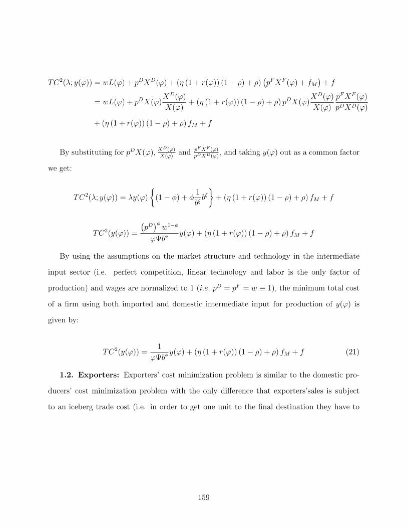
TC2(λ; y(ϕ)) = wL(ϕ) + pDXD(ϕ) + (η (1 + r(ϕ)) (1− ρ) + ρ)(pFXF (ϕ) + fM

)+ f

= wL(ϕ) + pDX(ϕ)XD(ϕ)

X(ϕ)+ (η (1 + r(ϕ)) (1− ρ) + ρ) pDX(ϕ)

XD(ϕ)

X(ϕ)

pFXF (ϕ)

pDXD(ϕ)

+ (η (1 + r(ϕ)) (1− ρ) + ρ) fM + f

By substituting for pDX(ϕ), XD(ϕ)X(ϕ)

and pFXF (ϕ)pDXD(ϕ)

, and taking y(ϕ) out as a common factor

we get:

TC2(λ; y(ϕ)) = λy(ϕ)

(1− φ) + φ

1

bξbξ

+ (η (1 + r(ϕ)) (1− ρ) + ρ) fM + f

TC2(y(ϕ)) =

(pD)φw1−φ

ϕΨbφy(ϕ) + (η (1 + r(ϕ)) (1− ρ) + ρ) fM + f

By using the assumptions on the market structure and technology in the intermediate

input sector (i.e. perfect competition, linear technology and labor is the only factor of

production) and wages are normalized to 1 (i.e. pD = pF = w ≡ 1), the minimum total cost

of a firm using both imported and domestic intermediate input for production of y(ϕ) is

given by:

TC2(y(ϕ)) =1

ϕΨbφy(ϕ) + (η (1 + r(ϕ)) (1− ρ) + ρ) fM + f (21)

1.2. Exporters: Exporters’ cost minimization problem is similar to the domestic pro-

ducers’ cost minimization problem with the only difference that exporters’sales is subject

to an iceberg trade cost (i.e. in order to get one unit to the final destination they have to

159

produce and ship τ units):

minLx(ϕ),Xx(ϕ),Xd

x(ϕ),XFx (ϕ),CD(ϕ)

TCx(ϕ, yx(ϕ)) = τwLx(ϕ) + τpDXdx(ϕ) + ρ

(τpFXF

x (ϕ) + fM)

+

(22)

+ fx + η (1 + r(ϕ))CDx (ϕ)

s.t. yx(ϕ) = ϕXx(ϕ)φLx(ϕ)1−φ (23)

Xx(ϕ) =[Xdx(ϕ)

ξ1+ξ + a

11+ξXF

x (ϕ)ξ

1+ξ

] 1+ξξ

(24)

Cx(ϕ) ≥ (1− ρ)(τpFXFx (ϕ) + fM) (25)

As bank loans are costly, exporters will demand bank loans equal to the amount of

total cost they cannot finance from own resources. Thus, the constraint in equation (25) is

binding. By plugging Cx(ϕ) into the objective function, the exporters’ cost minimization

problem becomes:

minLx(ϕ),Xx(ϕ),Xd

x(ϕ),XFx (ϕ)τwLx(ϕ) + τpDXd

x(ϕ) + τ (η (1 + r(ϕ)) (1− ρ) + ρ) pFXFx (ϕ) (26)

+ (η (1 + r(ϕ)) (1− ρ) + ρ) fM + fx

s.t. yx(ϕ) = ϕXx(ϕ)φLx(ϕ)1−φ (27)

Xx(ϕ) =[Xdx(ϕ)

ξ1+ξ + a

11+ξXF

x (ϕ)ξ

1+ξ

] 1+ξξ

(28)

The corresponding Lagrangean is:

160

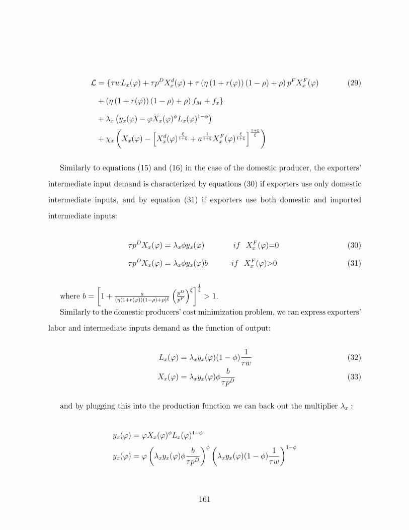
L = τwLx(ϕ) + τpDXdx(ϕ) + τ (η (1 + r(ϕ)) (1− ρ) + ρ) pFXF

x (ϕ) (29)

+ (η (1 + r(ϕ)) (1− ρ) + ρ) fM + fx

+ λx(yx(ϕ)− ϕXx(ϕ)φLx(ϕ)1−φ)

+ χx

(Xx(ϕ)−

[Xdx(ϕ)

ξ1+ξ + a

11+ξXF

x (ϕ)ξ

1+ξ

] 1+ξξ

)

Similarly to equations (15) and (16) in the case of the domestic producer, the exporters’

intermediate input demand is characterized by equations (30) if exporters use only domestic

intermediate inputs, and by equation (31) if exporters use both domestic and imported

intermediate inputs:

τpDXx(ϕ) = λxφyx(ϕ) if XFx (ϕ)=0 (30)

τpDXx(ϕ) = λxφyx(ϕ)b if XFx (ϕ)>0 (31)

where b =

[1 + a

(η(1+r(ϕ))(1−ρ)+ρ)ξ

(pD

pF

)ξ] 1ξ

> 1.

Similarly to the domestic producers’ cost minimization problem, we can express exporters’

labor and intermediate inputs demand as the function of output:

Lx(ϕ) = λxyx(ϕ)(1− φ)1

τw(32)

Xx(ϕ) = λxyx(ϕ)φb

τpD(33)

and by plugging this into the production function we can back out the multiplier λx :

yx(ϕ) = ϕXx(ϕ)φLx(ϕ)1−φ

yx(ϕ) = ϕ

(λxyx(ϕ)φ

b

τpD

)φ(λxyx(ϕ)(1− φ)

1

τw

)1−φ

161

From here it follows that λx is:

λx =τ

ϕΨ

(pD)φw1−φ

bφ

By using the normalization that w ≡ 1, and the assumptions on the technology and the

market structure in the intermediate input sectors that imply pD = pF = 1, the multiplier

λx becomes:

λx =τ

ϕΨbφ(34)

Thus, the minimum total cost, TCx(ϕ), resulting from the exporters’ cost minimization

problem is obtained by substituting (30)-(34) into the objective function (22):

TCx(ϕ) = τwLx(ϕ) + τpDXDx (ϕ) + τ (η (1 + r(ϕ)) (1− ρ) + ρ) pFXF

x (ϕ)

+ (η (1 + r(ϕ)) (1− ρ) + ρ) fM + f

Depending on whether the exporter uses or not imported intermediate inputs, we can

distinguish two case:

Case 1: If XFx (ϕ)=0 :

TC1x(λx; yx(ϕ)) = τwLx(ϕ) + τpDXD

x (ϕ) + fx

= λxyx(ϕ)(1− φ) + λxyx(ϕ)φ+ fx

= λxyx(ϕ) + f

By the perfect competition assumption in the intermediate input sector and the fact that

wages are normalized to 1 we get:

TC1x(yx(ϕ)) =

τ

ϕΨyx(ϕ) + fx (35)

162

Case 2: If XFx (ϕ)>0 :

TC2x(λx; yx(ϕ)) = τwLx(ϕ) + τpDXD

x (ϕ) + τ (η (1 + r(ϕ)) (1− ρ) + ρ)(pFXF

x (ϕ))

+ (η (1 + r(ϕ)) (1− ρ) + ρ) fM + f

= λxyx(ϕ)(1− φ) + λxyx(ϕ)φ

bξ

+ (η (1 + r(ϕ)) (1− ρ) + ρ)λxφyx(ϕ)pDξa

bξ [η (1 + r(ϕ)) (1− ρ) + ρ]1+ξ pFξ

+ [η (1 + r(ϕ)) (1− ρ) + ρ] fM + fx

TC2x(yx(ϕ)) =

τ

ϕΨbφyx(ϕ) + (η (1 + r(ϕ)) (1− ρ) + ρ) fM + fx (36)

2. Price setting:

Producers set prices by maximizing profit subject to demand and the total cost derived

from the cost minimization problem. Depending on whether the producers use domestic

and/or imported intermediate inputs, one can distinguish two cases when solves the profit

maximization problem both in the case of the domestic producers and exporters.

2.1. Domestic producer:

Case 1: XF (ϕ) = 0 :

maxp1(ϕ),y1(ϕ)

y1(ϕ)p1(ϕ)− TC1(y1(ϕ)

(37)

s.t. y1(ϕ) =Y

P

(p1(ϕ)

P

)−σ(38)

TC1(y(ϕ)) =1

ϕΨy1(ϕ) + f (39)

163

By plugging (38) and (39) into (37) we get:

maxp1(ϕ)

p1(ϕ)

Y

P

(p1(ϕ)

P

)−σ− 1

ϕΨ

Y

P

(p1(ϕ)

P

)−σ− f

(40)

The FOC associated to the optimization problem in (40) is:

Y

P 1−σ (1− σ)p1(ϕ)−σ +σY

ϕΨP 1−σ p1(ϕ)−σ−1 = 0 (41)

By plugging these back into (41), by using the demand function in (38) and the definition

of revenue, we get the price p1(ϕ), quantity supplied y1(ϕ) and the revenue q1(ϕ) generated

by the variety produced by the firm with productivity ϕ :

p1(ϕ) =σ

σ − 1

1

ϕΨ(42)

y1(ϕ) =Y

P 1−σ

[σ

σ − 1

1

ϕΨ

]−σ(43)

q1(ϕ) = p1(ϕ)y1(ϕ) =Y

P 1−σ

[σ

σ − 1

1

ϕΨ

]1−σ

(44)

Case 2: If XF (ϕ) > 0 :

maxp2(ϕ),y2(ϕ)

ηy2(ϕ)p2(ϕ)− TC2(y(ϕ)

(45)

s.t. y2(ϕ) =Y

P

(p2(ϕ)

P

)−σ(46)

TC2(y2(ϕ)) =1

ϕΨbφy2(ϕ) + (η (1 + r(ϕ)) (1− ρ) + ρ) fM + f (47)

By plugging (46) and (47) into (45), we get the unconstrained optimization problem:

164

maxp2(ϕ)

(ηp2(ϕ)− 1

ϕΨbφ

)Y

P

(p2(ϕ)

P

)−σ− (η (1 + r(ϕ)) (1− ρ) + ρ) fM − f

(48)

The FOC is: [η(1− σ) +

σ

ϕΨbφp2(ϕ)

]Y

P 1−σ p2(ϕ)−σ = 0 (49)

from which the following price p2(ϕ), quantity supplied y2(ϕ) and revenue results q2(ϕ) :

p2(ϕ) =σ

η (σ − 1)

1

ϕΨ

1

bφ(50)

y2(ϕ) =Y

P 1−σ

[σ

η (σ − 1)

1

ϕΨ

1

bφ

]−σ(51)

q2(ϕ) = p2(ϕ)y2(ϕ) =Y

P 1−σ

(σ

η (σ − 1)

1

ϕΨbφ

)1−σ

(52)

2.2. Exporter:

Case 1: If XFx (ϕ) = 0 :

maxp1x(ϕ),y1

x(ϕ)

y1x(ϕ)p1

x(ϕ)− TC1x(y1

x(ϕ)

(53)

s.t. y1x(ϕ) =

YxPx

(p1x(ϕ)

Px

)−σ(54)

TC1x(y1

x(ϕ)) =τ

ϕΨy1x(ϕ) + fx (55)

By plugging in the demand function:

maxp1x(ϕ)

p1x(ϕ)

YxPx

(p1x(ϕ)

Px

)−σ− τ

ϕΨ

YxPx

(p1x(ϕ)

Px

)−σ− fx

(56)

The FOC:

YxP 1−σx

(1− σ)p1x(ϕ)−σ +

τσ

ϕΨ

YxP 1−σx

p1x(ϕ)−σ−1 = 0 (57)

165

(1− σ +

τσ

ϕΨp1x(ϕ)

)YxP 1−σx

p1x(ϕ)−σ = 0 (58)

from which the following price p1x(ϕ), quantity y1

x(ϕ) and revenue q1x(ϕ) result:

p1x(ϕ) =

σ

σ − 1

τ

ϕΨ(59)

y1x(ϕ) =

YxP 1−σx

[σ

σ − 1

τ

ϕΨ

]−σ(60)

q1x(ϕ) = p1

x(ϕ)y1x(ϕ) =

YxP 1−σx

[σ

σ − 1

τ

ϕΨ

]1−σ

(61)

Case 2 : If XFx (ϕ) > 0 :

maxp2x(ϕ),y2

x(ϕ)

ηy2

x(ϕ)p2x(ϕ)− TCx(y2

x(ϕ)

(62)

s.t. y2x(ϕ) =

YxPx

(p2x(ϕ)

Px

)−σ(63)

TC2x(y2

x(ϕ)) =τ

ϕΨbφyx(ϕ) + (η (1 + r(ϕ)) (1− ρ) + ρ) fM + fx (64)

By plugging in the demand function:

maxp2x(ϕ)

ηp2x(ϕ)Yx

Px

(p2x(ϕ)Px

)−σ− τϕΨbφ

YxPx

(p2x(ϕ)Px

)−σ− (η (1 + r(ϕ)) (1− ρ) + ρ) fM − fx

(65)

The FOC: (η(1− σ) +

τσ

ϕΨbφp2x(ϕ)

)YxP 1−σx

p2x(ϕ)−σ = 0 (66)

from which the following price p2x(ϕ), quantity y2

x(ϕ) and revenue q2x(ϕ) result:

p2x(ϕ) =

σ

η (σ − 1)

τ

ϕΨbφ(67)

166

y2x(ϕ) =

Y

P 1−σ

[σ

η (σ − 1)

τ

ϕΨbφ

]−σ(68)

q2x(ϕ) = p2

x(ϕ)y2x(ϕ) =

Y

P 1−σ

(σ

η (σ − 1)

τ

ϕΨbφ

)1−σ

(69)

3. Material costs and profits by the four frm types:

3.1. Domestic producer:

Case 1: XF (ϕ) = 0

Material costs: the total material cost of the domestic producer using domestic interme-

diate input only:

pDXD(ϕ) = φ

(pD)φw1−φ

ϕΨbφY

P 1−σ

[σ

σ − 1

1

Ψϕ

]−σ(70)

= φY

P 1−σ

(σ

σ − 1

)−σ (1

ϕΨ

)1−σ

The profits by definition is:

π1(ϕ) = p1(ϕ)y1(ϕ)− pDXD(ϕ)− f (71)

and by plugging in the p1(ϕ), y1(ϕ) and pDXD(ϕ) from (42), (43) and (70), we get:

π1(ϕ) =Y

σP 1−σ

(σ

σ − 1

1

ϕΨ

)1−σ

− f (72)

This profit function written with respect to revenue is:

π1(ϕ) =1

σq1(ϕ)− f (73)

Case 2: XF (ϕ) > 0 :

167

Material costs: the total material cost of the firm using both domestic and imported

intermediate input is given by:

pDXD(ϕ) + pFXF (ϕ) (74)

= pDX(ϕ)XD(ϕ)

X(ϕ)+ pDX(ϕ)

XD(ϕ)

X(ϕ)

pFXF (ϕ)

pDXD(ϕ)

= pDX(ϕ)XD(ϕ)

X(ϕ)

(1 +

pFXF (ϕ)

pDXD(ϕ)

)= λφy2(ϕ)

1

bξ

(1 +

pFXF (ϕ)

pDXD(ϕ)

)=

φ

ϕΨ

1 + a((1+r∗)(1−ρ)+ρ)1+ξ(

1 + a((1+r∗)(1−ρ)+ρ)ξ

)φξ

+1y2(ϕ)

By using (51), the expression in (74) can be rewritten as:

pDXD(ϕ) + pFXF (ϕ) (75)

=φ

ϕΨ

1 + a((1+r∗)(1−ρ)+ρ)1+ξ(

1 + a((1+r∗)(1−ρ)+ρ)ξ

)φξ

+1

Y

P 1−σ

[σ

η (σ − 1)

1

ϕΨbφ

]−σ

The profit by defiition is:

π2(ϕ) = ηp2(ϕ)y2(ϕ)− 1

ϕΨbφy2(ϕ)− ((1 + r∗) (1− ρ) + ρ) fM − f (76)

By plugging (50) and (51) into (76), the following profit function results:

π2(ϕ) =η

σ

Y

P 1−σ

[σ

η (σ − 1)

1

ϕΨbφ

]1−σ

− ((1 + r∗) (1− ρ) + ρ) fM − f (77)

which can be rewritten in terms of the revenue by using the expression from (52):

π2(ϕ) =η

σq2(ϕ)− ((1 + r∗) (1− ρ) + ρ) fM − f (78)

168

3.2. Exporters:

Case 1: XF (ϕ) = 0

Material costs: the production for the export markets (79.1) and the total production

(79.2) in the case of exporters imply the following material costs:

τpDXDx (ϕ) = φ

τ

ϕΨ

YxP 1−σx

[σ

σ − 1

τ

ϕΨ

]−σ= φ

Y

P 1−σ

(τ

ϕΨ

)1−σ (σ

σ − 1

)−σ(79.1)

τpDXDx (ϕ) + pDXD(ϕ) = φ

Y

P 1−σ

(τ

ϕΨ

)1−σ (σ

σ − 1

)−σ+ φ

Y

P 1−σ

(σ

σ − 1

)−σ (1

ϕΨ

)1−σ

(79.2)

= φY

P 1−σ

(σ

σ − 1

)−σ (1

ϕΨ

)1−σ (1 + τ 1−σ)

The profit by definition is:

π1x(ϕ) = (N − 1) p1

x(ϕ)y1x(ϕ)− pDXD

x (ϕ)− fx (80)

By plugging (59), (60) into (80) and collecting terms, we get the profit function:

π1x(ϕ) =

(N − 1)Y

σP 1−σ

(σ

σ − 1

τ

ϕΨ

)1−σ

− fx (81)

which can be re-written in terms of the revenue by using the expression from (61):

π1x(ϕ) =

(N − 1)

σq1x(ϕ)− fx (82)

Case 2: If XF (ϕ) > 0 :

Material costs: of the exporters using both domestic and imported intermediate inputs

169

is:

τ(pDXD

x (ϕ) + pFXFx (ϕ)

)(83)

= τpDXx(ϕ)XDx (ϕ)

Xx(ϕ)+ τpDXx(ϕ)

XDx (ϕ)

Xx(ϕ)

pFXFx (ϕ)

pDXDx (ϕ)

= τpDXx(ϕ)XDx (ϕ)

Xx(ϕ)

(1 +

pFXFx (ϕ)

pDXDx (ϕ)

)

= λxφy2x(ϕ)b

XDx (ϕ)

Xx(ϕ)

(1 +

pFXFx (ϕ)

pDXDx (ϕ)

)= λxφy

2x(ϕ)

1

bξ

(1 +

a

(η (1 + r(ϕ)) (1− ρ) + ρ)1+ξ

)=

φτ

ϕΨ

1 + a((1+r∗)(1−ρ)+ρ)1+ξ(

1 + a((1+r∗)(1−ρ)+ρ)ξ

)1+φ

ξ

y2x(ϕ)

=1 + a

((1+r∗)(1−ρ)+ρ)1+ξ(1 + a

((1+r∗)(1−ρ)+ρ)ξ

)1+φ

ξ

Y

P 1−σ

[σ

η (σ − 1)

τ

ϕΨbφ

]−σφτ

ϕΨ

τ(pDXD

x (ϕ) + pFXFx (ϕ)

)+ pDXD(ϕ) + pFXF (ϕ) (84)

=φ

ϕΨ

1 + a((1+r∗)(1−ρ)+ρ)1+ξ(

1 + a((1+r∗)(1−ρ)+ρ)ξ

)φξ

+1y2(ϕ) +

φτ

ϕΨ

1 + a((1+r∗)(1−ρ)+ρ)1+ξ(

1 + a((1+r∗)(1−ρ)+ρ)ξ

)1+φ

ξ

y2x(ϕ)

=φ

ϕΨ

1 + a((1+r∗)(1−ρ)+ρ)1+ξ(

1 + a((1+r∗)(1−ρ)+ρ)ξ

)φξ

+1

Y

P 1−σ

[σ

η (σ − 1)

1

ϕΨbφ

]−σ (1 + τ 1−σ)

The profit by definition is:

π2x(ϕ) = η (N − 1) p2

x(ϕ)y2x(ϕ)− τ

ϕΨbφy2x(ϕ)− (η (1 + rx(ϕ)) (1− ρ) + ρ) fM − fx (85)

By using the expressions in (67) and (68), the resulting profit function is:

170

π2x(ϕ) = η

(N − 1)Y

σP 1−σ

(σ

η (σ − 1)

τ

ϕΨbφ

)1−σ

− (1 + r∗) (1− ρ) + ρ) fM − fx (86)

can be rewritten in terms of the revenue in (69) as:

π2x(ϕ) =

η

σq2x(ϕ)− (1 + r∗) (1− ρ) + ρ) fM − fx (87)

4. Material cost to sales (MS) and sales to value added (SV A) ratios:

4.1.1. Domestic producer using only domestic input:

MS1 =pDxD(ϕ)

q1(ϕ)=φ YP 1−σ

(σσ−1

)−σ ( 1ϕΨ

)1−σ

YP 1−σ

[σσ−1

1ϕΨ

]1−σ = φσ − 1

σ(88)

V AS1 = 1−MS1 = 1− φσ − 1

σ(89)

4.1.2. Domestic producer using domestic and imported intermediate input:

MS2 =pDxD(ϕ) + pFxF (ϕ)

p2(ϕ)y2(ϕ)=

φϕΨ

1+ a

((1+r∗)(1−ρ)+ρ)1+ξ(1+ a

((1+r∗)(1−ρ)+ρ)ξ

)φξ

+1y2(ϕ)

p2(ϕ)y2(ϕ)(90)

=

φϕΨ

1+ a

((1+r∗)(1−ρ)+ρ)1+ξ(1+ a

((1+r∗)(1−ρ)+ρ)ξ

)φξ

+1

ση(σ−1)

1ϕΨ

1bφ

= ηφσ − 1

σ

1 + a((1+r∗)(1−ρ)+ρ)1+ξ

1 + a((1+r∗)(1−ρ)+ρ)ξ

V AS2 = 1−MS2 = 1− ηφσ − 1

σ

1 + a((1+r∗)(1−ρ)+ρ)1+ξ

1 + a((1+r∗)(1−ρ)+ρ)ξ

(91)

4.1.3. Exporters using domestic intermediate input have material cost generated by the

export to sales ratio as described in (92.1), while total material cost to sales ratio as described

171

in (92.2):

MS1x =

τpDxXDx (ϕ)

q1x(ϕ)

=λxφy

1x(ϕ)

p1x(ϕ)y1

x(ϕ)=

λxφ

p1x(ϕ)

(92.1)

=λxφ

p1x(ϕ)

=φ τϕΨ

σ(σ−1)

τϕΨ

= φσ − 1

σ

MS1 =τpDXD

x (ϕ) + pDXD(ϕ)

q1(ϕ) + q1x(ϕ)

=φ YP 1−σ

(σσ−1

)−σ ( 1ϕΨ

)1−σ(1 + τ 1−σ)

YP 1−σ

[σσ−1

1ϕΨ

]1−σ+ Yx

P 1−σx

[σσ−1

τϕΨ

]1−σ (92.2)

= φσ − 1

σ

These imply a value added to sales ratio:

V AS1x = 1−MS1

x = 1− φσ − 1

σ= 1−MS1 (93)

4.1.4. Exporters using domestic and imported intermediate input:

The material cost implied by export sales to share ratio in the case of exporters is given

by (94.1), while the total material cost to sales ratio is given by (94.2):

MS2x =

τ(pDXD

x (ϕ) + pFXFx (ϕ)

)q2x(ϕ)

=

φτϕΨ

1+ a

((1+r∗)(1−ρ)+ρ)1+ξ(1+ a

((1+r∗)(1−ρ)+ρ)ξ

)1+φξ

y2x(ϕ)

p2x(ϕ)y2

x(ϕ)(94.1)

=φ

1+ a

((1+r∗)(1−ρ)+ρ)1+ξ

1+ a

((1+r∗)(1−ρ)+ρ)ξ

σηx(σ−1)

= ηφσ − 1

σ

1 + a((1+r∗)(1−ρ)+ρ)1+ξ

1 + a((1+r∗)(1−ρ)+ρ)ξ

172

MS2 =pDxD(ϕ) + pFxF (ϕ) + τ

(pDXD

x (ϕ) + pFXFx (ϕ)

)q2(ϕ) + q2

x(ϕ)(94.2)

= φ

1+ a

((1+r∗)(1−ρ)+ρ)1+ξ(1+ a

((1+r∗)(1−ρ)+ρ)ξ

)φξ

+1+

1+ a

((1+r∗)(1−ρ)+ρ)1+ξ(1+ a

((1+r∗)(1−ρ)+ρ)ξ

)φξ

+1τ 1−σ

ση(σ−1)

1bφ

+ ση(σ−1)

τ1−σ

bφ

= ηφσ − 1

σ

1 + a((1+r∗)(1−ρ)+ρ)1+ξ

1 + a((1+r∗)(1−ρ)+ρ)ξ

Thus, the value added to sales ratio is:

V AS2x = 1−MS2

x = 1− ηφσ − 1

σ

1 + a((1+r∗)(1−ρ)+ρ)1+ξ

1 + a((1+r∗)(1−ρ)+ρ)ξ

(95)

= 1−MS2

5. Productivity cutoffs:

We define cutoff productivities ϕ1, ϕ2, ϕ3, ϕ1x, ϕ

2x, ϕ

3x such that in case (i) ∀ϕ ∈ (0, ϕ1)

productivity draw firms decide to exit the market, ∀ϕ ∈ (ϕ1, ϕ1x) firms stay in the market,

produce and sell on the domestic market by using domestic intermediate input only, ∀ϕ ∈

(ϕ1x, ϕ

2x) firms start to export by using domestic intermediate input only, ∀ϕ ∈ (ϕ2

x, 1) firms

sell on the domestic market and export by using both domestic and imported intermediate

inputs; in case (ii) ∀ϕ ∈ (0, ϕ2) productivity draw firms decide to exit the market, ∀ϕ ∈

(ϕ2, ϕ3) firms stay in the market, produce and sell on the domestic market by using only

domestic intermediate input, ∀ϕ ∈ (ϕ3, ϕ3x) firms stay in the market, produce and sell on

the domestic market by using both domestic and imported intermediate inputs, ∀ϕ ∈ (ϕ3x, 1)

firms start to export by using both domestic and imported intermediate inputs.

In case (i) the three cutoff productivities ϕ1, ϕ1x, ϕ

2x are pinned down by the following

173

system of equations:

π1(ϕ1) = 0 (96)

π1(ϕ1x) = π1(ϕ1

x) + π1x(ϕ

1x) (97)

π1(ϕ2x) + π1

x(ϕ2x) = π2(ϕ2

x) + π2x(ϕ

2x) (98)

fe = [G(ϕ2x)−G(ϕ1)]

∑∞t=0(1− δ)t

E

[1

σq1(ϕ)− f

]+ (99)

+ [G(ϕ2x)−G(ϕ1

x)]∑∞

t=00(1− δ)tE

[N − 1

σq1x(ϕ)]− fx

]+

+ [1−G(ϕ2x)]∑∞

t=0(1− δ)tE

[1

σq2(ϕ) +

N − 1

σq2x(ϕ)− fx − f − ((1 + r∗)(1− ρ) + ρ)fM

]

where equation (96) is the zero profit condition for producing for the domestic market

such that firms with productivity draw ϕ1 are indifferent between producing, selling on the

domestic market and making profit π1(ϕ1); equation (97) states that firms with productivity

draw ϕ1x are indifferent between producing by using only domestic intermediates, selling on

the domestic market and making π1(ϕ1x) and producing by using only domestic intermediates,

selling on both domestic and export markets with profit π1(ϕ1x)+π1

x(ϕ1x); equation (98) states

that firms with ϕ2x are indifferent between producing for both the domestic and export market

by using domestic intermediate input only and making π1(ϕ2x) + π1

x(ϕ2x), and producing for

both markets by using both domestic and imported intermediate inputs making π2(ϕ2x) +

π2x(ϕ

2x) profit; equation (99) is the free entry condition according to which firms that decide

to enter the market must get in expectation at least as much profit that covers the sunk cost

of entry, fe, based on which they learn their productivity.

By using the definition of profits we derived in (72), (77), (81) and (87), the equations

174

(96) - (99) can be rewritten:

Y

σP 1−σ

(σ

σ − 1

1

ϕ1Ψ

)1−σ

= f (96’)

(N − 1)Y

σP 1−σ

(σ

σ − 1

τ

ϕ1xΨ

)1−σ

= fx (97’)

Y

σP 1−σ

[σ

(σ − 1)

1

ϕ2xΨ

]1−σ (1 + (N − 1)τ 1−σ) [ησbφ(σ−1) − 1

](98’)

= ((1 + r∗) (1− ρ) + ρ) fM

From (96’) and (97’) it follows that:

ϕ1x

ϕ1 = τ

(fx

(N − 1)f

) 1σ−1

(100)

From (97’) and (98’) it follows after some algebraic manipulations that:

ϕ2x

ϕ1x

=1

τ

(((1 + r∗) (1− ρ) + ρ) fM

fx (ησbφ(σ−1) − 1) (1 + (N − 1)τ 1−σ)

) 1σ−1

(101)

From(96’) and (98’) it follows after some algebraic manipulation that:

ϕ2x

ϕ1 =

(((1 + r∗) (1− ρ) + ρ) fM

(N − 1)f(1 + (N − 1)τ 1−σ) (ησbφ(σ−1) − 1)

) 1σ−1

(102)

By using equations (100), (102) and (99), we compute ϕ1 as the function of model

parameters as follows:

(i) We compute the discounted sums by using that∑∞

t=0(1− δ)t = 1δ

and substituting it

175

to (99):

[G(ϕ2x)−G(ϕ1)]

1

δE

[1

σq1(ϕ)− f

]+ [G(ϕ2

x)−G(ϕ1x)]

1

δE

[N − 1

σq1x(ϕ)]− fx

]+

+ [1−G(ϕ2x)]

1

δE

[1

σq2(ϕ) +

N − 1

σq2x(ϕ)− fx − f − ((1 + r∗)(1− ρ) + ρ)fM

]= fe

(ii) We compute the expected values as follows:

E

[1

σq1(ϕ)− f

]=∫ ϕ2

x

ϕ1

[1

σq1(ϕ)− f

]g(ϕ)

[G(ϕ2x)−G(ϕ1)]

dϕ

E

[N − 1

σq1x(ϕ)− fx

]=∫ ϕ1

x

ϕ1

[N − 1

σq1x(ϕ)− fx

]g(ϕ)

[G(ϕ2x)−G(ϕ1

x)]dϕ

E

[1

σq2(ϕ) +

N − 1

σq2x(ϕ)− fx − f − ((1 + r∗)(1− ρ) + ρ)fM

]=∫∞ϕ2x

[1

σq2(ϕ) +

N − 1

σq2x(ϕ)− fx − f − ((1 + r∗)(1− ρ) + ρ)fM

]g(ϕ)

[1−G(ϕ2x)]dϕ

and substitute them into the equation in (i) we get:

∫ ϕ2x

ϕ1

[1

σq1(ϕ)− f

]g(ϕ)dϕ+

∫ ϕ1x

ϕ1

[N − 1

σq1x(ϕ)− fx

]g(ϕ)dϕ+

+∫∞ϕ2x

[1

σq2(ϕ) +

N − 1

σq2x(ϕ)− fx − f − ((1 + r∗)(1− ρ) + ρ)fM

]g(ϕ)dϕ = δfe

(iii) By substituting the Pareto pdf g(ϕ) = kϕkmϕk+1 and the revenue functions q1(ϕ), q1

x(ϕ),

q2(ϕ) and q2x(ϕ) from (44), (52), (61) and (69), we compute the LHS of the expression in

176

(ii):

1

σ

Y

P 1−σkϕkm

k − (σ − 1)

(σ

(σ − 1)ψ

)1−σ [(ϕ1)(σ−1)−k −

(ϕ2x

)(σ−1)−k]

+1

σ

Y

P 1−σkϕkm

k − (σ − 1)

(σ

(σ − 1)ψ

)1−σ

(N − 1)τ 1−σ[(ϕ1x

)(σ−1)−k −(ϕ2x

)(σ−1)−k]

+1

σ

Y

P 1−σkϕkm

k − (σ − 1)

(σ

η (σ − 1)ψbφ

)1−σ [(ϕ2x

)(σ−1)−k+ (N − 1)τ 1−σ (ϕ2

x

)(σ−1)−k]

= δfe + f [1−G(ϕ1)] + fx[1−G(ϕ1x)] + ((1 + r∗)(1− ρ) + ρ)fM [1−G(ϕ2

x)]

(iv) By using the expressions for ϕ1x/ϕ

1 and ϕ2x/ϕ

1, the expression for Y/P 1−σ = fσ/

(ϕ1)σ−1(

σ(σ−1)ψ

)1−σresulted from (96) and the Pareto cdf G(ϕ) = 1−

(ϕmϕ

)k, we can write

the equation in (iii) in terms of ϕ1 :

fk

k − (σ − 1)

[1−

(((1 + r∗) (1− ρ) + ρ) fM

(N − 1)f(1 + (N − 1)τ 1−σ) (ησbφ(σ−1) − 1)

) (σ−1)−kσ−1

] (ϕ1)−k

+τfk(N − 1)τ 1−σ

k − (σ − 1)

(fx

(N − 1)f

) (σ−1)−kσ−1 (

ϕ1)−k

− fk(N − 1)τ 1−σ

k − (σ − 1)

(((1 + r∗) (1− ρ) + ρ) fM

(N − 1)f(1 + (N − 1)τ 1−σ) (ησbφ(σ−1) − 1)

) (σ−1)−kσ−1 (

ϕ1)−k

+fk (1 + (N − 1)τ 1−σ)

k − (σ − 1)

(ηbφ)σ−1

[(((1 + r∗) (1− ρ) + ρ) fM

(N − 1)f(1 + (N − 1)τ 1−σ) (ησbφ(σ−1) − 1)

) (σ−1)−kσ−1

] (ϕ1)−k

=δfeϕkm

+ f(ϕ1)−k

+ fx

(τ

(fx

(N − 1)f

) −kσ−1

) (ϕ1)−k

+ ((1 + r∗)(1− ρ) + ρ)fM

(((1 + r∗) (1− ρ) + ρ) fM

(N − 1)f(1 + (N − 1)τ 1−σ) (ησbφ(σ−1) − 1)

) −kσ−1 (

ϕ1)−k

We solve for ϕ1 by denoting the terms independent of r∗ by ∆ in order to simplify

notation:

(ϕ1)k

= ∆1 + ∆2

(ησbφ(σ−1) − 1

((1 + r∗) (1− ρ) + ρ) fM

) k−(σ−1)σ−1

∆3ησbφ(σ−1) + ∆4

177

where ∆1 = ϕkmδfe

f(σ−1)k−(σ−1)

+ ϕkmδfe

[(N−1)f ]k

σ−1

(fx)(σ−1)−kσ−1

[k

(k−(σ−1))τσ− τ],

∆2 = ϕkmδfe

(N − 1)f (1 + (N − 1)τ 1−σ) [(N − 1)f(1 + (N − 1)τ 1−σ)]k−(σ−1)σ−1 ,

∆3 = ϕkmδfe

(k−η(N−1)(k−(σ−1))η(N−1)(k−(σ−1))

),∆4 = ϕkm

δfe

(N−1)(k−(σ−1))−k(N−1)(k−(σ−1))

.

(v) Once we solved for ϕ1, we can easily solve for ϕ1x and ϕ2

x by using equations (100)

and (102).

In case (ii), the three cutoff productivities ϕ2, ϕ3, ϕ3x are pinned down by the following

system of equations:

π1(ϕ2) = 0 (104)

π1(ϕ3) = π2(ϕ3) (105)

π2(ϕ3x) = π2(ϕ3

x) + π2x(ϕ

3x) (106)

− fe + [G(ϕ3)−G(ϕ2)]∑∞

t=0(1− δ)tE

[1

σq1(ϕ)− f

]+ (107)

+ [1−G(ϕ3)]∑∞

t=0(1− δ)tE

[1

σq2(ϕ)− f − ((1 + r∗)(1− ρ) + ρ)fM

]+

+ [1−G(ϕ3x)]∑∞

t=0(1− δ)tE

[N − 1

σq2x(ϕ)− fx

]= 0

where equation (104) is the zero profit condition for producing for the domestic market

such that firms with productivity draw ϕ2 are indifferent between selling on the domestic

market and exiting; equation (105) states that firms with productivity draw ϕ3 are indifferent

between using only domestic intermediate inputs and selling on the domestic market, and

using both inputs and selling on the domestic market; equation (106) states that firms with

ϕ3x are indifferent between producing for the domestic market by using both intermediate

inputs, and producing for both markets by using both domestic and imported intermediate

inputs. Equation (107) is the free entry condition.

178

By using the definition of profits we derived in (73), (77), (82) and (87), the equations

(104) - (106) can be rewritten:

Y

σP 1−σ

(σ

σ − 1

1

ϕ2Ψ

)1−σ

= f (104’)

Y

σP 1−σ

(σ

σ − 1

1

ϕ3Ψ

)1−σ

=η

σ

Y

P 1−σ

[σ

η (σ − 1)

1

ϕ3Ψbφ

]1−σ

− ((1 + r∗) (1− ρ) + ρ) fM

(105’)

η(N − 1)Y

σP 1−σ

(σ

η (σ − 1)

τ

ϕ3xΨb

φ

)1−σ

= (1 + r∗) (1− ρ) + ρ) fM + fx (106’)

From (104’) and (105’) it follows that:

ϕ3

ϕ2 =

(((1 + r∗) (1− ρ) + ρ) fM

f (ησbφ(σ−1) − 1)

) 1σ−1

(108)

From (104’) and (106’) it follows after some algebraic manipulations that:

ϕ3x

ϕ2 =

(((1 + r∗) (1− ρ) + ρ) fM + fx

f(N − 1)ησbφ(σ−1)τ 1−σ

) 1σ−1

(109)

From(105’) and (106’) it follows after some algebraic manipulation that:

ϕ3x

ϕ3 =

((((1 + r∗) (1− ρ) + ρ) fM + fx)

(ησbφ(σ−1) − 1

)((1 + r∗) (1− ρ) + ρ) fM(N − 1)ησbφ(σ−1)τ 1−σ

) 1σ−1

(110)

By using equations (107), (108) and (109), we compute ϕ2 as the function of model

parameters as follows:

(i) We compute the discounted sums by using that∑∞

t=0(1− δ)t = 1δ

and substituting it

to (107):

179

[G(ϕ3)−G(ϕ2)]1

δE

[1

σq1(ϕ)− f

]+

+ [1−G(ϕ3)]1

δE

[1

σq2(ϕ)− f − ((1 + r∗)(1− ρ) + ρ)fM

]+

+ [1−G(ϕ3x)]

1

δE

[N − 1

σq2x(ϕ)− fx

]= fe

(ii) We compute the expected values as follows:

E

[1

σq1(ϕ)− f

]=∫ ϕ3

ϕ2

[1

σq1(ϕ)− f

]g(ϕ)

[G(ϕ3)−G(ϕ2)]dϕ

E

[1

σq2(ϕ)− f − ((1 + r∗)(1− ρ) + ρ)fM

]=∫∞ϕ3

[1

σq2(ϕ)− f − ((1 + r∗)(1− ρ) + ρ)fM

]g(ϕ)

[1−G(ϕ3)]dϕ

E

[N − 1

σq2x(ϕ)− fx

]=∫∞ϕ3x

[N − 1

σq2x(ϕ)− fx

]g(ϕ)

[1−G(ϕ3x)]dϕ

and substitute them into the expression in (i) we get:

1

σ

∫ ϕ3

ϕ2 q1(ϕ)g(ϕ)dϕ+

1

σ

∫∞ϕ3 q

2(ϕ)g(ϕ)dϕ+N − 1

σ

∫∞ϕ3xq2x(ϕ)g(ϕ)dϕ

= δfe +(1−G(ϕ2)

)f + fx

(1−G(ϕ3

x))

+ ((1 + r∗)(1− ρ) + ρ)fM(1−G(ϕ3))

(iii) By substituting the Pareto pdf g(ϕ) = kϕkmϕk+1 and the revenue functions q1(ϕ), q1

x(ϕ),

q2(ϕ) and q2x(ϕ) from (44), (52), (61) and (69), we compute the LHS of the expression in

180

(ii):

Y

σP 1−σ

∫ ϕ3

ϕ2

[σ

σ − 1

1

ϕψ

]1−σ

g(ϕ)dϕ+Y

σP 1−σ

∫∞ϕ3

(σ

η (σ − 1)

1

ϕψbφ

)1−σ

g(ϕ)dϕ

+(N − 1)Y

σP 1−σ

∫∞ϕ3x

(σ

η (σ − 1)

τ

ϕψbφ

)1−σ

g(ϕ)dϕ

= δfe + ϕkm(ϕ2)kf + ϕkm(ϕ3x)kfx + ϕkm(ϕ3)k((1 + r∗)(1− ρ) + ρ)fM

Y

σP 1−σkϕkm

k − (σ − 1)

(σ

(σ − 1)ψ

)1−σ (ϕ2)(σ−1)−k −

(ϕ3)(σ−1)−k

+

Y

σP 1−σkϕkm

k − (σ − 1)

(σ

η (σ − 1)ψbφ

)1−σ (ϕ3)(σ−1)−k

+(N − 1)Y

σP 1−σkϕkm

k − (σ − 1)

(σ

η (σ − 1)

τ

ψbφ

)1−σ (ϕ3x

)(σ−1)−k

= δfe + ϕkm(ϕ2)kf + ϕkm(ϕ3x)kfx + ϕkm(ϕ3)k((1 + r∗)(1− ρ) + ρ)fM

(iv) By using the expressions for ϕ1x/ϕ

1 and ϕ2x/ϕ

1, and the expression for Y/P 1−σ = fσ/

(ϕ2)σ−1(

σ(σ−1)ψ

)1−σresulted from (104), we can write the equation in (iii) in terms of ϕ2 :

fk

k − (σ − 1)

1−

(((1 + r∗) (1− ρ) + ρ) fM

f (ησbφ(σ−1) − 1)

) (σ−1)−kσ−1

+fk

k − (σ − 1)

(ηbφ)σ−1

(((1 + r∗) (1− ρ) + ρ) fM

f (ησbφ(σ−1) − 1)

) (σ−1)−kσ−1

+(N − 1) fk

k − (σ − 1)

(ηbφ

τ

)σ−1(((1 + r∗) (1− ρ) + ρ) fM + fx

f(N − 1)ησbφ(σ−1)τ 1−σ

) (σ−1)−kσ−1

=δfeϕkm

(ϕ2)k

+ f +

(((1 + r∗) (1− ρ) + ρ) fM + fx

f(N − 1)ησbφ(σ−1)τ 1−σ

) −kσ−1

fx

+

(((1 + r∗) (1− ρ) + ρ) fM

f (ησbφ(σ−1) − 1)

) −kσ−1

((1 + r∗)(1− ρ) + ρ)fM

We solve for ϕ2 by denoting the terms independent of r∗ in order to simplify notation26:

26k((1 + r∗) (1− ρ) + ρ) fM > −kfx (1− η)− fxη (σ − 1) always holds.

181

(ϕ2)k

= ∆5 + ∆6

(ησbφ(σ−1) − 1

) kσ−1

[((1 + r∗) (1− ρ) + ρ) fM ]k−(σ−1)σ−1

+ ∆7bφk

[((1 + r∗) (1− ρ) + ρ) fM + fx]k

σ−1

k (((1 + r∗) (1− ρ) + ρ) fM + fx)

fxη (k − (σ − 1))− 1

∆5 = ϕkmδfe

f(σ−1)k−(σ−1)

, ∆6 = ϕkmδfef

kσ−1 σ−1

k−(σ−1), ∆7 = fx [f (N − 1)]

kσ−1 τ−kη

σkσ−1 .

(v) Once we solved for ϕ2, we can easily solve for ϕ3 and ϕ3x by using equations (108)

and (109).

6. Comparative statics:

Proof of Proposition 1:

From (90) we know that the material to sales ratio of the producers using both do-

mestic and imported intermadiate inputs is a function of r∗ and it is given by MS2 =

ηφσ−1σ

1+ a

((1+r∗)(1−ρ)+ρ)1+ξ

1+ a

((1+r∗)(1−ρ)+ρ)ξ

Change in the materials to sales ratio with respect to the change in r is given by (denote

z ≡ ((1 + r∗) (1− ρ) + ρ)):

dMS2

dr∗=

∂

∂r∗

(ηφσ − 1

σ

1 + az−1−ξ

1 + az−ξ

)= ηφ

σ − 1

σ

(−1− ξ)az−2−ξ (1− ρ)(1 + az−ξ

)+ ξaz−1−ξ(1− ρ)(1 + az−1−ξ)

(1 + az−ξ)2

= ηφ(σ − 1) (1− ρ)az−1−ξ

σz(1 + az−ξ)2

[(−1− ξ)(1 + az−ξ) + ξz(1 + az−1−ξ)

]= ηφ

(σ − 1) (1− ρ)az−1−ξ

σz(1 + az−ξ)2

[−1− ξ − a

zξ+ ξz

]

The sign of this expression depends on the sign of the −1 − ξ − azξ

+ ξz. If this latter

expression is negative, then dMS2/dr∗ < 0. This happens if ξz < 1 + ξ + azξ. By using our

notation, this is equivalent to bξ + ξ(1 − z) > 0. By plugging in z, we get bξ + ξ(1 − z) =

bξ− ξ (1− ρ) r∗.By using our assumption that 1+ ξ > 1, bξ > 1, 1−ρ ∈ (0, 1) and r∗ ∈ [0, 1],

182

it follows that if ξ ∈ (0, 1). This implies that ξ (1− ρ) r∗ ∈ (0, 1) and bξ > ξ (1− ρ) r∗. This

implies ξz < 1 + ξ + azξ

holds. Thus, we showed that dMS2/dr∗ < 0

Proof of Corollary 1

Notice from Section 2.4 that V AS = 1−MS. Thus, the derivative of the sales to value

added ratio with respect to r∗ is:

dV AS2

dr∗=∂V AS2

∂MS2

∂MS2

∂r∗= −∂MS2

∂r∗

As it has been shown that dMS2/dr∗ < 0, it follows that dV AS2/dr∗ > 0

Proof of Proposition 2

From equations (90) and (94.2) we know that the material to sales ratio of the producers

using both domestic and imported intermadiate inputs is a function of r∗ and it is given by

MS2 = ηφσ−1σ

1+ a

((1+r∗)(1−ρ)+ρ)1+ξ

1+ a

((1+r∗)(1−ρ)+ρ)ξ.From the proof of Proposition 1 we know that dMS2/dr∗ <

0. From equations (88) and (92.2) we know that the material to sales ratio of the producers

using domestic intermadiate inputs only is MS1 = φσ−1σ.Thus, dMS1/dr∗ = 0, and it follows

that |dMS2/dr∗ | < |dMS1/dr∗| .

By using the identity that V AS = 1−MS, it follows that |dV AS2/dr∗ | > |dV AS1/dr∗|

Proof of Proposition 3

case (i)

Let A1 ≡(

ησbφ(σ−1)−1((1+r∗)(1−ρ)+ρ)fM

) k−(σ−1)σ−1

. As k > 0, sign(d (ϕ1) /dr∗) = sign(d(

(ϕ1)k)/dr∗

).

d((ϕ1)

k)

dr∗= ∆2

dA1

dr∗

∆3η

σbφ(σ−1) + ∆4

+ ∆2A1∆3η

σφ (σ − 1) bφ(σ−1)−1 d(b)dr∗.

dA1

dr∗= k−(σ−1)

σ−1A1

[ησφ(σ−1)bφ(σ−1)−1

ησbφ(σ−1)−1

d(b)dr∗− (1−ρ)

(1+r∗)(1−ρ)+ρ)

], which sign depends on d(b)

dr∗as k >

(σ − 1) , A1 > 0 and ησφ(σ−1)bφ(σ−1)−1

ησbφ(σ−1)−1> 0 given our assumptions on σ and η. We know that

b =

[1 + a

((1+r∗)(1−ρ)+ρ)ξ

(pD

pF

)ξ] 1ξ

. Thus, d(b)dr∗

= − a(1−ρ)b

(a+((1+r∗)(1−ρ)+ρ)ξ)((1+r∗)(1−ρ)+ρ)< 0 given

our assumptions of ρ ∈ (0, 1). Thus, dA1

dr∗< 0 and d(b)

dr∗< 0 imply that

d((ϕ1)

k)

dr∗< 0.

183

Now, we compute (ϕ2x)k

by substituting (ϕ1)k

into:

(ϕ2x)k

= (ϕ1)k

(((1+r∗)(1−ρ)+ρ)fM

(N−1)f(1+(N−1)τ1−σ)(ησbφ(σ−1)−1)

) kσ−1

= ∆1

[(N−1)f(1+(N−1)τ1−σ)]k

σ−1

(((1+r∗)(1−ρ)+ρ)fM

(ησbφ(σ−1)−1)

) kσ−1

+ ∆2

[(N−1)f(1+(N−1)τ1−σ)]k

σ−1

(((1+r∗)(1−ρ)+ρ)fM

ησbφ(σ−1)−1

)∆3η

σbφ(σ−1) + ∆4

As k > 0, sign(d (ϕ2

x) /dr∗) = sign

(d(

(ϕ2x)k)/dr∗

). Let A2 =

(((1+r∗)(1−ρ)+ρ)fM

(ησbφ(σ−1)−1)

) kσ−1

and A3 = ((1+r∗)(1−ρ)+ρ)fMησbφ(σ−1)−1

. Thus,d((ϕ2

x)k)

dr∗is given by:

d((ϕ2

x)k)

dr∗= ∆1

[(N−1)f(1+(N−1)τ1−σ)]k

σ−1

dA2

dr∗

+ ∆2

[(N−1)f(1+(N−1)τ1−σ)]k

σ−1

dA3

dr∗

∆3η

σbφ(σ−1) + ∆4

+∆2A3∆3η

σφ (σ − 1) bφ(σ−1)−1 d(b)dr∗

=∆1kA2(1−ρ)fM(ησbφ(σ−1)−1)

(ησbφ(σ−1)−1)((1+r∗)(1−ρ)+ρ)fM (σ−1)[(N−1)f(1+(N−1)τ1−σ)]k

σ−1

− ∆1kA2ησφ(σ−1)bφ(σ−1)−1A3

((1+r∗)(1−ρ)+ρ)fM (σ−1)[(N−1)f(1+(N−1)τ1−σ)]k

σ−1

d(b)dr∗

+∆2∆3ησbφ(σ−1)+∆4(1−ρ)fM

(ησbφ(σ−1)−1)[(N−1)f(1+(N−1)τ1−σ)]k

σ−1

+∆2A3∆3ησφ (σ − 1) bφ(σ−1)−1

(1−

ησbφ(σ−1)+

∆4∆3

(ησbφ(σ−1)−1)

1

[(N−1)f(1+(N−1)τ1−σ)]k

σ−1

)d(b)dr∗

.

We know that

dA2

dr∗= k

σ−1A2

(ησbφ(σ−1)−1)((1+r∗)(1−ρ)+ρ)fM

(1−ρ)fM(ησbφ(σ−1)−1)−((1+r∗)(1−ρ)+ρ)fMησφ(σ−1)bφ(σ−1)−1 d(b)

dr∗

(ησbφ(σ−1)−1)2 > 0

since d(b)dr∗

< 0.

dA3

dr∗=

(1−ρ)fM(ησbφ(σ−1)−1)−((1+r∗)(1−ρ)+ρ)fMησφ(σ−1)bφ(σ−1)−1 d(b)

dr∗

(ησbφ(σ−1)−1)2 > 0 since d(b)

dr∗< 0

andησbφ(σ−1) + ∆4

∆3

>(ησbφ(σ−1) − 1

)[(N − 1)f(1 + (N − 1)τ 1−σ)]

kσ−1 by our assump-

tions on the parameters.Thus,d((ϕ2

x)k)

dr∗> 0.

As k > 0, sign(d (ϕ2) /dr∗) = sign(d(

(ϕ2)k)/dr∗

).Denoting A5 = bφk

[((1+r∗)(1−ρ)+ρ)fM+fx]k

σ−1

and A6 =(ησbφ(σ−1)−1)

kσ−1

[((1+r∗)(1−ρ)+ρ)fM ]k−(σ−1)σ−1

, (ϕ2)k

becomes:

(ϕ2)k

= ∆5 + ∆6A6 + ∆7A5

k(((1+r∗)(1−ρ)+ρ)fM+fx)

fxη(k−(σ−1))− 1

. By taking the derivative with

respect to r∗ :

d((ϕ2)

k)

dr∗= ∆6

dA6

dr∗+∆7

dA5

dr∗

k(((1+r∗)(1−ρ)+ρ)fM+fx)

fxη(k−(σ−1))− 1

+∆7A5k(1−ρ)fM

fxη(k−(σ−1))+∆7A5

k(1−ρ)fMfxη(k−(σ−1))

= ∆6dA6

dr∗+ ∆7

φkbφk−1

[((1+r∗)(1−ρ)+ρ)fM+fx]k

σ−1

d(b)dr∗

184

−∆7kbφkfM (1−ρ)

(σ−1)[((1+r∗)(1−ρ)+ρ)fM+fx]k−(σ−1)σ−1

k(((1+r∗)(1−ρ)+ρ)fM+fx)

fxη(k−(σ−1))− 1

+∆7bφk

[((1+r∗)(1−ρ)+ρ)fM+fx]k

σ−1

k(1−ρ)fMfxη(k−(σ−1))

We already showed that dA1

dr∗< 0, d(b)

dr∗< 0. We compute and sign

dA5

dr∗=

φkbφk−1

[((1 + r∗) (1− ρ) + ρ) fM + fx]k

σ−1

d (b)

dr∗−

bφk kσ−1

(1 + r∗) (1− ρ)

[((1 + r∗) (1− ρ) + ρ) fM + fx]k−(σ−1)σ−1

< 0

since d(b)dr∗

< 0.

Also, we compute and sign

dA6

dr∗=

kσ−1(ησbφ(σ−1)−1)

kσ−1−1

ησφ(σ−1)bφ(σ−1)−1

[((1+r∗)(1−ρ)+ρ)fM ]k−(σ−1)σ−1

d(b)dr∗− k−(σ−1)

σ−1

(ησbφ(σ−1)−1)k

σ−1 (1−ρ)fM

[((1+r∗)(1−ρ)+ρ)fM ]k

σ−1< 0 since

d(b)dr∗

< 0. Based on this we can easily see thatd((ϕ2)

k)

dr∗< 0 since fxη (k − (σ − 1)) <

σ−1)((1+r∗)(1−ρ)+ρ)fM+fx

+ k (((1 + r∗) (1− ρ) + ρ) fM + fx) always hold as

k (((1 + r∗) (1− ρ) + ρ) fM + fx) > fxη (k − (σ − 1))

under case 1 productivity ranking.

We compute (ϕ3)k

as follows:

(ϕ3)k

= (ϕ2)k

(((1+r∗)(1−ρ)+ρ)fM

f(ησbφ(σ−1)−1)

) kσ−1

= ∆5A2 + ∆6fM

fk

σ−1((1 + r∗) (1− ρ) + ρ) + ∆7A7

[k(((1+r∗)(1−ρ)+ρ)fM+fx)

fxη(k−(σ−1))− 1]

where A2 =

(((1+r∗)(1−ρ)+ρ)fM

f(ησbφ(σ−1)−1)

) kσ−1

, A7 = bφk[((1+r∗)(1−ρ)+ρ)fM ]k

σ−1

fk

σ−1 (ησbφ(σ−1)−1)k

σ−1 [((1+r∗)(1−ρ)+ρ)fM+fx]k

σ−1

.

We compute the derivative:

d((ϕ3)

k)

dr∗= ∆5

dA2

dr∗+ ∆6

fM

fk

σ−1(1− ρ)

+∆7dA7

dr∗

[k(((1+r∗)(1−ρ)+ρ)fM+fx)

fxη(k−(σ−1))− 1]

+ ∆7A7k(1−ρ)fM

fxη(k−(σ−1))

We already showed that dA2

dr∗> 0 and based on our assumption on the model parameters

we know that ∆6fM

fk

σ−1(1− ρ) > 0 and ∆7A7

k(1−ρ)fMfxη(k−(σ−1))

> 0.

dA7

dr∗= φkbφk−1[((1+r∗)(1−ρ)+ρ)fM ]

kσ−1

fk

σ−1 (ησbφ(σ−1)−1)k

σ−1 [((1+r∗)(1−ρ)+ρ)fM+fx]k

σ−1

d(b)dr∗

+k

σ−1bφk[((1+r∗)(1−ρ)+ρ)fM ]

kσ−1−1

(1−ρ)fMf

fk

σ−1 (ησbφ(σ−1)−1)k

σ−1 [((1+r∗)(1−ρ)+ρ)fM+fx]k

σ−1

185

− bφk[((1+r∗)(1−ρ)+ρ)fM ]k

σ−1 kσ−1(ησbφ(σ−1)−1)

−1ησφ(σ−1)bφ(σ−1)−1

fk

σ−1 (ησbφ(σ−1)−1)k

σ−1 [((1+r∗)(1−ρ)+ρ)fM+fx]k

σ−1

d(b)dr∗

− bφk[((1+r∗)(1−ρ)+ρ)fM ]k

σ−1 kσ−1

[((1+r∗)(1−ρ)+ρ)fM+fx]−1(1−ρ)fM

fk

σ−1 (ησbφ(σ−1)−1)k

σ−1 [((1+r∗)(1−ρ)+ρ)fM+fx]k

σ−1

Since ησbφ(σ−1)−1ησbφ(σ−1)−1

+ 1ησbφ(σ−1)−1

> 1 and ((1+r∗)(1−ρ)+ρ)fM+fx((1+r∗)(1−ρ)+ρ)fM

> ησbφ(σ−1)

ησbφ(σ−1)−1under case (ii)

ranking, it follows that dA7

dr∗> 0. Thus,

d((ϕ3)

k)

dr∗> 0.

We compute (ϕ3x)k

as follows:

(ϕ3x)k

= ∆5

(((1+r∗)(1−ρ)+ρ)fM+fxf(N−1)ησbφ(σ−1)τ1−σ

) kσ−1

+∆6

(1

f(N−1)τ1−σ

) ( ησbφ(σ−1)−1

ησbφ(σ−1)

) kσ−1

(((1+r∗)(1−ρ)+ρ)fM+fx)k

σ−1

[((1+r∗)(1−ρ)+ρ)fM ]k−(σ−1)σ−1

+ ∆7

[f(N−1)ηστ1−σ ]k

σ−1bk−(σ−1)

k(((1+r∗)(1−ρ)+ρ)fM+fx)

fxη(k−(σ−1))− 1

= ∆5A8 + ∆6

(1

f(N−1)τ1−σ

)A9

+ ∆7

[f(N−1)ηστ1−σ ]k

σ−1bk−(σ−1)

k(((1+r∗)(1−ρ)+ρ)fM+fx)

fxη(k−(σ−1))− 1

The derivatived((ϕ3

x)k)

dr∗is given by:

d((ϕ3

x)k)

dr∗= ∆5

dA8

dr∗+ ∆6

(1

f(N−1)τ1−σ

)dA9

dr∗

+∆7(k−(σ−1))bk−(σ−1)−1

[f(N−1)ηστ1−σ ]k

σ−1

k(((1+r∗)(1−ρ)+ρ)fM+fx)

fxη(k−(σ−1))− 1

d(b)dr∗

+ ∆7bk−(σ−1)

[f(N−1)ηστ1−σ ]k

σ−1

k(1−ρ)fMfxη(k−(σ−1))

where

dA8

dr∗= k

σ−1

(((1+r∗)(1−ρ)+ρ)fM+fxf(N−1)ησbφ(σ−1)τ1−σ

) kσ−1−1 (1−ρ)fMf(N−1)ησbφ(σ−1)τ1−σ−f(N−1)ηστ1−σφ(σ−1)bφ(σ−1)−1 d(b)

dr∗

(f(N−1)ησbφ(σ−1)τ1−σ)2

> 0.

dA9

dr∗=

(((1+r∗)(1−ρ)+ρ)fM+fx)k

σ−1 kσ−1

(ησbφ(σ−1)−1

ησbφ(σ−1)

) kσ−1−1

φ(σ−1)bφ(σ−1)−1−φ(σ−1)b−1(ησbφ(σ−1)−1)

ησbφ(σ−1)

[((1+r∗)(1−ρ)+ρ)fM ]k−(σ−1)σ−1

d(b)dr∗

+(1−η−σb−φ(σ−1))

kσ−1 k

σ−1(((1+r∗)(1−ρ)+ρ)fM+fx)

kσ−1−1

(1−ρ)fM

[((1+r∗)(1−ρ)+ρ)fM ]k−(σ−1)σ−1

− (k−(σ−1))(1−ρ)fM(1−η−σb−φ(σ−1))k

σ−1 (((1+r∗)(1−ρ)+ρ)fM+fx)k

σ−1

(σ−1)[((1+r∗)(1−ρ)+ρ)fM ]k

σ−1> 0

since bφ(σ−1) > ησbφ(σ−1) − 1 and ((k−(σ−1)))[((1+r∗)(1−ρ)+ρ)fM ]k(((1+r∗)(1−ρ)+ρ)fM+fx)

> 1 in case (ii) productivity

ranking

A.2 Data Appendix

1. Confidential micro data

186

1.1. The balance sheet data at the firm level are coming from the Hungarian Central

Statistical Office. The data are collected by the Hungarian Fiscal Authority based on the

annual Financial Reports that firms with double-entry bookkeeping must submit at the end

of each fiscal year (end of December of the calendar year). The financial reports contain

information on balance sheets and income statements of all operating firms in Hungary with

double-entry bookkeeping. In this paper we use the following variables at firm-year unit of

observation:

Industry: each firm reports a 4-digit NACE industry code based on its main economic

activity; Sales: the total domestic and export sales reported in 1000 Hungarian forints, at

current prices; Materials: total cost of material reported in 1000 Hungarian forints, at current

prices; Value added: computed as the difference between total sales and material costs in

1000 Hungarian forints, at current prices; Accounts payable: total obligations to pay off as

short-term debt to non-bank creditors reported in 1000 Hungarian forints, at current prices;

Short term credit: total obligations to pay off as short-term debt to bank creditors reported

in 1000 Hungarian forints, at current prices; Accounts receivable: payments expected to

receive for the outstanding amounts reported in 1000 Hungarian forints, at current prices;

Number of employees: number of workers employed by the firm in a given year.

1.2. Data on the international trade transactions of the Hungarian manufacturing firms

are from the Hungarian Central Statistical Office. These data were collected by the Hun-

garian Custom Authority covering the whole universe of international trade transactions

conducted by Hungarian firms. These data are reported at the firm level for each product

classified at the 8-digit combined nomenclature (CN) in values and weights, for each country

of origin/destination. The focus of this paper is on the following variables at firm-year-

product-country of origin/destination unit of observation:

Country of origin/destination: country the imported product originates from in the

case of imports or destination country of products shipped in the case of exports; Product

code: combined nomenclature (CN) product code reported at the eight-digit level. CN

187

code is a European product classification with the first 6-digits corresponding to the World

Harmonized System (HS-6); Import: total value of imports reported in 1000 Hungarian

forints, at current prices; Export sales: total export sales reported in 1000 Hungarian forints,

at current prices.

1.3. Bank Account Numbers Data on firms’ current account numbers are from a Hungar-

ian private data provider, Wolters Kluwer Complex Kiado. The data is collected from the

Hungarian Business Registry administered by the Hungarian Registry Court. The data are

reported at the firm level and contain all the current account numbers of the firms, the date

it was opened and closed in mm/dd/yy format. I use the first three numbers of the 24-digit

current account number, in order to determine the bank at which the current account was

opened. These numbers provide the GIRO code of the bank, the unique bank identifier set

by the National Bank of Hungary.

2. Publicly available data.

1. Input-Output Tables

We use the Input-Output tables from year 2000 published by the Hungarian Central

Statistical Office with 74 NACE 2-digit industry codes to identify firms in manufacturing

sectors with 2 digit NACE codes ranging from 15 to 36.

2. Product Concordances

Imported intermediate inputs: are defined by using the correspondences27 between the

Harmonized Commodity Description and Coding System, and Broad Economic Categories

from the United Nations Intermediate Goods in Trade Statistics28. First, we create a con-

cordance between the CN8 product codes reported in the Trade Data and the HS6 product

codes used in the UN concordance tables which provides the BEC code for each HS6. I

define intermediate imported input as the product with BEC codes: 111, 121, 21, 22, 31,

322, 42, 53.

27For more details: http://unstats.un.org/unsd/cr/registry/regot.asp28For more details: http://unstats.un.org/unsd/tradekb/Knowledgebase/Intermediate-Goods-in-Trade-

Statistics

188

3. Bank-level panel data

I use annual reports of the Hungarian Banking Association, the Hungarian Financial Su-

pervisory Authority and the National Bank of Hungary on the development of the Hungarian

financial sector to trace the ownership structure of the whole universe of commercial banks

operating in Hungary between 1992-2006 by the unique GIRO identifier. I define a bank

with domestic ownership if the previously listed reports provide the information that more

than 50% of the banks’ shares were owned by Hungarian owner in a given year. Similarly,

if more than 50% of the shares of the bank are owned by foreigners, I defined the bank as

foreign owned.

By using the bank level panel data combined with the GIRO numbers recovered from

the Bank Account Number data, we define two types of firms: firms banking with domestic

banks and firms banking with foreign banks. Based on this, we define the following three

dummy variables:

Banking with domestic bank only : variable takes value one if the firm had current account

opened only at banks with domestic ownership and 0 otherwise; Banking with foreign bank

only : variable takes value one if the firm had current account opened only at banks with

foreign ownership and zero otherwise; Banking with both foreign and domestic bank : variable

takes value one if the firm had current account opened at both types of banks and zero

otherwise.

We obtain the dataset used in the paper by merging the dataset on firms’ balance sheets,

international trade transactions and bank accounts based on the unique fiscal firm identifier,

which then we merge to the bank-level panel data based on the unique bank identifier. We

restrict the dataset to the sample of manufacturing firm and years 1998-2002. Manufacturing

industries are defined according to NACE 2-digit industry codes ranging from 15 to 36 (i.e.

excluding wholesalers, mining, services).

A.3 Results Appendix

189

Table 1.1 Average ratios by firms over the period 1998 - 2002

Banking with domes-

tic bank only

Banking with foreign

bank only

Banking with both foreign

and domestic bank

Value added to sales 0.395 0.349 0.192

Material cost to sales 0.605 0.651 0.818

Short term loan to sales 0.180 0.162 0.134

Payables to sales 0.130 0.141 0.175

Receivables to sales 0.163 0.176 0.147

Short term loan to material 0.299 0.249 0.248

Payables to material 0.216 0.217 0.214

Observations 30,691 25,921 45,933

Table 1.2 Average ratios by firms over the period 1998 - 2002

All Importer

Value added to sales 0.314 0.341

Material cost to sales 0.690 0.695

Short term loan to sales 0.157 0.173

Payables to sales 0.082 0.083

Receivables to sales 0.176 0.191

Short term loan to material 0.224 0.248

Payables to material 0.118 0.118

Import to sales na 0.244

Imported intermediate to sales na 0.186

Observations 102,545 25,636

190

Table 2.1 The impact of liberalization on production and sales decisions - Baseline estimates

∆(Value added

to sales)it

∆(Value added

to sales)it

∆(Materials

to sales)it

∆(Materials

to sales)it

(1) (2) (3) (4)

DB onlyi,2001 -0.022** -0.022** 0.027*** 0.027***

[0.009] [0.009] [0.008] [0.008]

ln(empl)i,2001 0.003 0.003 0.025*** 0.025***

[0.002] [0.002] [0.003] [0.003]

∆ln(empl)i,t 0.031 -0.002

[0.006] [0.007]

Industry FE yes yes yes yes

Observations 9,047 9,047 9,050 9,050

Note: The dependent variables are expressed in level changes of ratios in 2002 relative to the pre-

liberalization period, 2000. Banking with domestic bank onlyi,2001 is a dummy taking 1 if the firms did

banking with domestic banks only in 2001. [] standard errors clustered at four-digit industry level; ***

significant at 1%, ** significant at 5%. The estimation is based on a balanced panel of manufacturing firms.

191

Table 2.2 The impact of liberalization on financing decisions - Baseline estimates

Dependent

variable

∆(Short

term loan

to sales)it

∆(Short

term loan

to sales)it

∆(Payables

to sales)it

∆(Payables

to sales)it

∆(Recei -

vables to

sales)it

∆(Recei -

vables to

sales)it

(1) (2) (3) (4) (5) (6)

DB onlyi,2001 0.039*** 0.039*** -0.001 -0.001 -0.004 -0.004

[0.014] [0.014] [0.002] [0.002] [0.007] 0.007

ln(empl)i,2001 -0.006** -0.005** 0.0004 0.0004 -0.003*** -0.003***

[0.003] [0.003] [0.001] [0.001] [0.001] [0.001]

∆ln(empl)i,t -0.047*** 0.001 -0.018***

[0.011] [0.002] [0.004]

Industry FE yes yes yes yes yes yes

Observations 9,061 9,061 9,052 9,052 9,050 9,050

Note: The dependent variables are expressed in level changes of ratios in 2002 relative to the pre-liberalization

period, 2000. Banking with domestic bank onlyi,2001 is a dummy taking 1 if the firms did banking with

domestic banks only in 2001. [] robust standard errors clustered at four-digit industry level; *** significant

at 1%, ** significant at 5%. The estimation is based on a balanced panel of manufacturing firms.

192

Table 2.3 The impact of liberalization on financing decisions - Baseline estimates

Dependent variable ∆(Short term loan

to material cost)it

∆(Short term loan

to material cost)it

∆(Payables to

material cost)it

∆(Payables to

material cost)it

(1) (2) (3) (4)

DB onlyi,2001 0.084** 0.084** -0.008** -0.008**

[0.036] [0.036] [0.004] [0.004]

ln(empl)i,2001 -0.018 -0.017 –0.002** -0.002**

[0.012] [0.011] [0.001] [0.001]

∆ln(empl)i,t -0.094*** 0.003

[0.034] [0.003]

Industry FE yes yes yes yes

Observations 9,042 9,042 9,011 9,011

Note: The dependent variables are expressed in level changes of ratios in 2002 relative to the pre-liberalization

period, 2000. Banking with domestic bank onlyi,2001 is a dummy taking 1 if the firms did banking with

domestic banks only in 2001. [] robust standard errors clustered at four-digit industry level; *** significant

at 1%, ** significant at 5%. The estimation is based on a balanced panel of manufacturing firms.

193

Table 3.1 The impact of liberalization on production and sales decisions - Importers

Dependent

variable

∆(Import

to sales)it

∆(Import

to sales)it

∆(Imported

input to

sales)it

∆(Imported

input to

sales)it

∆(Domestic

input to

sales)it

∆(Domestic

input to

sales)it

(1) (2) (3) (4) (5) (6)

DB onlyi,2001 0.016** 0.016** 0.017*** 0.017*** 0.002 0.003

[0.008] [0.008] [0.006] [0.006] [0.011] [0.011]

ln(empl)i,2001 0.0004 0.001 -0.001 -0.001 0.004 0.004

[0.002] [0.002] [0.002] [0.002] [0.003] [0.003]

∆ln(empl)i,t 0.025*** 0.018*** -0.031

[0.007] [0.005] [0.019]

Industry FE yes yes yes yes yes yes

Obs 2,614 2,614 2,614 2,614 2,614 2,614

Note: The dependent variables are expressed in level changes of ratios in 2002 relative to the pre-liberalization

period, 2000. Banking with domestic bank onlyi,2001 is a dummy taking 1 if the firms did banking with

domestic banks only in 2001. [] robust standard errors clustered at four-digit industry level; *** significant

at 1%, ** significant at 5%. The estimation is based on a balanced panel of manufacturing firms.

194

Table 3.2 The impact of financial liberalization on financing decisions - Importers

Dependent

variable

∆(Short

term loan

to sales)it

∆(Short

term loan

to sales)it

∆(Payables

to sales)it

∆(Payables

to sales)it

∆(Recei-

vables to

sales)it

∆(Recei-

vables to

sales)it

(1) (2) (3) (4) (5) (6)

DB onlyi,2001 0.027** 0.028** 0.004 0.004 -0.011 -0.009

[0.012] [0.012] [0.005] [0.005] [0.012] [0.012]

ln(empl)i,2001 0.004 0.004 -0.0002 -0.0002 -0.010** -0.010**

[0.003] [0.003] [0.002] [0.001] [ 0.005] [0.004]

∆ln(empl)i,t -0.048*** -0.003 -0.065***

[0.015] [0.005] [0.015]

Industry FE yes yes yes yes yes yes

Observations 2,537 2,537 2,479 2,479 2,537 2,537

Note: The dependent variables are expressed in level changes of ratios in 2002 relative to the pre-liberalization

period, 2000. Banking with domestic bank onlyi,2001 is a dummy taking 1 if the firms did banking with

domestic banks only in 2001. [] robust standard errors clustered at four-digit industry level; *** significant

at 1%, ** significant at 5%. The estimation is based on a balanced panel of manufacturing firms.

195

Table 3.3 The impact of financial liberalization on financing decisions - Importers

Dependent

variable

∆(Short term loan

to material cost)it

∆(Short term loan

to material cost)it

∆(Payables to

material cost)it

∆(Payables to

material cost)it

(1) (2) (3) (4)

DB onlyi,2001 0.042** 0.043** 0.001 0.001

[0.019] [0.019] [0.008] [0.010]

ln(empl)i,2001 0.003 0.003 -0.002 -0.002

[0.006] [0.006] [0.002] [0.002]

∆ln(empl)i,t -0.051** 0.004

[0.023] [0.007]

Industry FE yes yes yes yes

Observations 2,525 2,525 2,532 2,532

Note: The dependent variables are expressed in level changes of ratios in 2002 relative to the pre-liberalization

period, 2000. Banking with domestic bank onlyi,2001 is a dummy taking 1 if the firms did banking with

domestic banks only in 2001. [] robust standard errors clustered at four-digit industry level; *** significant

at 1%, ** significant at 5%. The estimation is based on a balanced panel of manufacturing firms.

196

Table 4 The impact of financial liberalization on firms’ input imports market entry decisions

Dependent variable P(It>0|It-1=0) P(It>0|It-1=0) P(It>0|It-1=0) P(It>0|It-1=0)

OLS OLS Probit Probit

(1) (2) (3) (4)

DB onlyi,2001 0.014*** 0.013** 0.149*** 0.151***

[0.005] [0.006] [0.051] [0.051]

ln(empl)i,2001 0.006 0.006 0.061*** 0.062***

[0.002] [0.002] [0.017] [0.017]

∆ln(empl)i,t 0.0227*** 0.253***

[0.0045] [0.046]

Industry FE yes yes yes yes

Obs 10,403 10,403 10,403 10,403

Note: The dependent variable takes value one if the firm became an importer in 2002 relative to 2000, and

zero otherwise. Banking with domestic bank onlyi,2001 is a dummy taking 1 if the firms did banking with

domestic banks only in 2001. *** significant at 1%, ** significant at 5%.

197

Table5.1Alternativedenitionofthetreatementgroup-wholesample

Dependent

variable

(Valueadded

tosales)it

(Materials

tosales)it

(Short

term

loantosales)it

(Payables

tosales)it

(Receivables

tosales)it

(Shortterm

loan

tomaterialcost) it

(Payablesto

materialcost) it

(1)

(2)

(3)

(4)

(5)

(6)

(7)

DBi;2001

-0.020***

0.016***

0.035***

-0.001

0.001

0.066*

-0.007**

[0.006]

[0.005]

[0.010]

[0.002]

[0.004]

[0.037]

[0.003]

ln(empl) i;2001

0.003***

0.023***

-0.004***

-0.00003

-0.002***

-0.006

-0.002***

[0.001]

[0.002]

[0.002]

[0.0004]

[0.0007]

[0.006]

[0.0007]

ln(empl) i;t

0.028***

-0.001

-0.048***

0.0008

-0.015***

-0.099***

0.003***

[0.004]

[0.004]

[0.006]

[0.001]

[0.003]

[0.025]

[0.001]

Obs

16,026

16,071

16,074

16,059

16,046

16,061

16,056

Table5.2Alternativedenitionofthetreatementgroup-importes

Dependent

variable

(Importto

sales)it

(Importedin-

puttosales)it

(Domesticin-

puttosales)it

(Short

term

loan

tosales)it

(Payables

tosales)it

(Receivables

tosales)it

(Shortterm

loan

tomater-

ialcost) it

(Payables

tomaterial

cost) it

(1)

(2)

(3)

(4)

(5)

(6)

(7)

(8)

DBi;2001

0.005

0.008**

0.0005

0.029**

-0.001

-0.003

0.030**

-0.003

[0.005]

[0.004]

[0.007]

[0.014]

[0.004]

[0.006]

[0.013]

[0.005]

ln(empl) i;2001

-0.0007

-0.0006

0.004**

-0.007**

0.00005

-0.003***

-0.002

-0.0005

[0.001]

[0.001]

[0.002]

[0.003]

[0.0008]

[0.001]

[0.003]

[0.001]

ln(empl) i;t

0.018***

0.011***

-0.039**

-0.064***

-0.003

-0.030***

-0.037**

0.0004

[0.006]

[0.003]

[0.015]

[0.017]

[0.004]

[0.008]

[0.018]

[0.005]

Obs

4,057

4,057

3,310

3,942

3,839

3,839

3,921

3,921

Note:Thesamplecontainsabalancedpanelofmanufacturingrmsover1998-2002.Thedependentvariablesareexpressedaschangesintheratios

from

2000to2002.DBi;2001isadummytakingvalueoneifthermbankswithdomesticbanksin2001.[]standarderrorsclusteredatfourdigit

industrylevel.Industryxede¤ectsspeciedatfour-digitsindustrylevelareincluded.**,*signicantat5%,and10%.

63198

Table6Placebodi¤erence-in-di¤erenceestimates

Dependent

variable

(Value

added

tosales)it1

(Materials

tosales)it1

(Short

term

loan

tomaterial

cost) it1

(Importto

sales)it1

(Imported

input

to

sales)it1

(Domestic

input

to

sales)it1

(Short

term

loan

tomaterial

cost) it1

(1)

(2)

(3)

(4)

(5)

(6)

(7)

DBonlyi;2001

-0.007

0.004

-0.035

-0.003

-0.004

0.018**

0.012

[0.009]

[0.009]

[0.075]

[0.004]

[0.003]

[0.009]

[0.040]

ln(empl) i;2001

-0.004***

0.004***

0.0007

0.029***

0.027***

-0.022***

0.026

[0.001]

[0.001]

[0.012]

[0.002]

[0.002]

[0.002]

[0.019]

IndustryFE

yes

yes

yes

yes

yes

yes

yes

Obs

9,047

9,050

9,050

2,546

2,546

2,546

2,546

Note:Thesamplecontainsabalancedpanelofmanufacturingrmsover1998-2002.Thedependentvariablesareexpressedinlevelchangesofratios

in2000relativeto1998.DBonlyi;2001isadummytakingvalueoneifthermsdidbankingwithdomesticbanksonlyin2001.[]clusteredstandard

errorsatfour-digitsindustrylevel;***signicantat1%**signicantat5%

64199

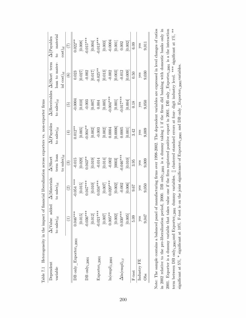
Table7.1Heterogeneityintheimpactofnancialliberalizationacrossexportersvs.non-exporterrms

Dependent

variable

(Value

added

tosales)it

(Materials

tosales)it

(Short

term

loan

tosales)it

(Payables

tosales)it

(Receivables

tosales)it

(Shortterm

loan

tomater-

ialcost) it

(Payables

tomaterial

cost) it

(1)

(2)

(3)

(4)

(5)

(6)

(7)

DBonly_Exporter i;2001

0.046***

-0.054***

-0.015

0.012**

-0.0004

0.023

0.022**

[0.015]

[0.015]

[0.029]

[0.005]

[0.010]

[0.027]

[0.008]

DBonlyi;2001

-0.036***

0.047***

0.043**

-0.004**

-0.003

-0.002

-0.015***

[0.012]

[0.010]

[0.019]

[0.002]

[0.007]

[0.017]

[0.004]

Exporter i;2001

-0.021***

0.034***

-0.014

-0.003

0.004

-0.025**

-0.013***

[0.007]

[0.007]

[0.014]

[0.002]

[0.005]

[0.013]

[0.003]

ln(empl) i;2001

0.005**

0.020***

-0.002

0.0004

-0.004***

-0.002

-0.0004

[0.002]

[0.002]

[0003]

[0.0006]

[0.001]

[0.003]

[0.001]

ln(empl) i;t

0.030***

-0.002

-0.046***

0.0005

-0.017***

-0.012

0.002

[0.005]

[0.006]

[0.010]

[0.001]

[0.004]

[0.009]

[0.002]

F-test

5.09

9.67

3.95

3.42

0.18

0.50

6.09

IndustryFE

yes

yes

yes

yes

yes

yes

yes

Obs

9,047

9,050

9,009

9,009

9,050

9,030

9,011

Note:Thesamplecontainsabalancedpanelofmanufacturingrmsover1998-2002.Thedependentvariablesareexpressedinlevelchangesofratios

in2002relativetothepre-liberalizationperiod,2000.DBonlyi;2001isadummytaking1ifthermsdidbankingwithdomesticbanksonlyin

2001.Exporterisadummyvariablethattakesvalueoneifthermregisteredpositiveexportin2001.DBonly_Exporter i;2001isatheinteraction

term

betweenDBonlyi;2001andExporter i;2001dummyvariables.[]clusteredstandarderrorsatfour-digitindustrylevel.***signicantat1%,**

signicantat5%,*signicantat10%.F-testisonthejointsignicanceofExporter i;2001andDBonly_Exporter i;2001variables.

65200

Table7.2Heterogeneityintheimpactofnancialliberalizationacrossexportersvs.non-exporterimporters

(Import

tosales)it

(Imported

inputto

sales)it

(Domestic

inputto

sales)it

(Short

term

loan

tosales)it

(Payables

tosales)it

(Receivables

tosales)it

(Shortterm

loan

tomater-

ialcost) it

(Payables

tomaterial

cost) it

(1)

(2)

(3)

(4)

(5)

(6)

(7)

(8)

DBonly_Exporter i;2001

0.015

0.016

-0.034

-0.021

0.012

-0.010

-0.075

0.026

[0.017]

[0.017]

[0.030]

[0.028]

[0.012]

[0.019]

[0.057]

[0.021]

DBonlyi;2001

0.006

0.002

0.038

0.041

-0.007

0.002

0.088

-0.018

[0.014]

[0.013]

[0.029]

[0.021]

[0.011]

[0.018]

[0.049]

[0.018]

Exporter i;2001

-0.017

-0.011

0.038**

0.009

-0.006

0.0007

0.008

-0.018**

[0.011]

[0.009]

[0.017]

[0.011]

[0.004]

[0.008]

[0.021]

[0.006]

ln(empl) i;2001

0.001

-0.0005

0.002

-0.0002

0.0001

-0.003

-0.003

0.0008

[0.003]

[0.002]

[0.005]

[0.003]

[0.001]

[0.002]

[0.006]

[0.001]

ln(empl) i;t

0.03***

0.025***

-0.079

-0.047***

-0.002

-0.028**

-0.035

0.0065

[0.009]

[0.006]

[0.031]

[0.013]

[0.005]

[0.010]

[0.024]

[0.006]

F-test

1.79

1.56

0.88

3.48

0.66

0.37

1.83

0.83

IndustryFE

yes

yes

yes

yes

yes

yes

yes

yes

Obs

2,733

2,733

2,733

2,849

2,799

2,855

2,858

2,798

Note:Thesamplecontainsmanufacturingrmsthatwereimportersin2001.Thedependentvariablesareexpressedinlevelchangesofratiosin2002

relativetothepre-liberalizationperiod,2000.DBonlyi;2001isadummytaking1ifthermsdidbankingwithdomesticbanksonlyin2001.Exporter

isadummyvariablethattakesvalueoneifthermregisteredpositiveexportin2001.DBonly_Exporter i;2001isatheinteractionterm

betweenDB

onlyi;2001andExporter i;2001dummyvariables.[]clusteredstandarderrorsatfour-digitindustrylevel.***signicantat1%,**signicantat5%,*

signicantat10%.F-testisonthejointsignicanceofExporter i;2001andDBonly_Exporter i;2001variables.

66201

Chapter 3

International Financial Adjustment in

a Canonical Open Economy Growth

Model

3.1 Introduction

In influential work, Gourinchas and Rey (2007) have shown that international financial

adjustment (IFA) in the expected returns on a country’s international investment portfolio

as well as the expected path of the real exchange rate can complement or even substitute

for the traditional adjustment channel via a narrowing of country’s ‘unsustainable’ current

account imbalance. In their paper, GR derive this result using a log linearization of a net

foreign asset accumulation identity without reference to any specific theoretical model of

international financial adjustment in expected foreign asset returns or the real exchange

rate. In this paper we calibrate the importance of IFA in a standard open economy growth

model (Schmitt-Grohe and Uribe, 2003) with a well-defined steady level of foreign liabilities.

In this model there is a country specific credit spread which varies as a function of the ratio

202

of foreign liabilities to GDP.1

We study a perfect foresight version of the model so that we can characterize the global

dynamic adjustment in net foreign assets, the endogenous cost of debt service, and the path

of the real exchange rate. This is important, because in this model, in a neighborhood of

the steady state, IFA is not very important. However, away from the steady state – we look

at simulations in which the initial stock of foreign debt is 10 percent above its steady state

ratio to GDP and the initial capital stock is 10 percent below its steady state ratio to GDP –

IFA is very important. In fact in our baseline simulation in which we calibrate the elasticity

of the country credit spread to the debt to GDP ratio based on plausible empirical estimates

from the literature as well as our own estimates, we find that allowing for an IFA channel

results in a very rapid converge of the current account to its steady state (relative to the

no IFA case) so that most of the time that the country is adjusting , all the adjustment is

via forecastable changes in the costs of servicing debt and in the appreciation real exchange

rate and none of the adjustment is in the current account. By contrast, in the no IFA

case, current account adjustment by construction does all the work and current account

adjustment is much slower. Finally we show that IFA adjustment via the real exchange rate

can be important even if forecastable changes in the cost of debt service are not.

This paper is related to three strands of the recent international finance literature. First,

it relates to the growing literature that studies the channels of international financial adjust-

ment (Gourinchas and Rey, 2007, 2013). We contribute to this literature by measuring the

relative importance of the trade and financial channels in a standard open economy growth

model (Schmitt-Grohe and Uribe, 2003) with a well-defined steady level of foreign liabilities.

This approach also sheds light on the mechanism through which the financial channel op-

erates that is the financial externality faced by the representative household while making

intertemporal borrowing decisions. Second, we contribute to the small open economy real

1Devereux and Sutherland (2010) examined this question in a two country model in which the excessreturn arises from a risk premium in an asset-choice problem. They concluded the valuation channel couldnot be important in such a model, at least in the neighborhood of a non-stochastic steady state.

203

business cycle literature that studies the importance of country spread in the business cycle

fluctuations of emerging economies (Mendoza, 1991; Schmitt-Grohe and Uribe, 2003, 2016;

Neumeyer and Perri, 2005; Garcia-Cicco et al., 2010). We provide structural estimates of the

elasticity of country spread with respect to the external debt position in the case of Central

and Eastern European countries that are quantitatively larger than the calibration used by

prior papers. However, our estimates are similar to the reduced form estimates found in

the finance literature (Cantor and Packer, 1996; Eichengreen and Mody, 1998; Rowland and

Torres, 2004; Hilscher and Nosbusch, 2010). Finally, we contribute to the quantitative real

business cycle literature that focuses on developing approximation methods to small-scale

DSGE models. We show that by solving for the global dynamics of the model under per-

fect foresight, without log-linearizing it, interesting non-linearities can be captured in the

external adjustment of the small open economy in the long-run.

The rest of this chapter is organized as follows. Section 3.2 discusses the channels of

international adjustment. Section 3.3 presents the theoretical framework, and Section 3.4

discusses the calibration. Section 3.5 presents the simulation results, while Section 3.6 con-

cludes.

3.2 Channels of the Small Open Economy’s Interna-

tional Financial Adjustment

Countries can stabilize their net international investment position through two channels: the

trade channel and the financial channel. As net foreign liabilities today must be compensated

by trade surpluses in the future, the trade channel contributes to the external adjustment

of the country by the adjustment in the value of the goods and services that the country

imports or exports. However, the forecastable increase in the real returns on the net foreign

assets or forecastable decrease in the real cost of servicing net international liabilities (i.e.

the financial channel) can substitute for adjustment in trade flows. Thus, the financial

204

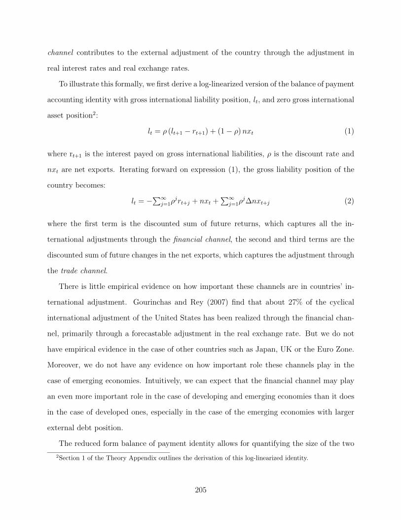
channel contributes to the external adjustment of the country through the adjustment in

real interest rates and real exchange rates.

To illustrate this formally, we first derive a log-linearized version of the balance of payment

accounting identity with gross international liability position, l t, and zero gross international

asset position2:

lt = ρ (lt+1 − rt+1) + (1− ρ)nxt (1)

where rt+1 is the interest payed on gross international liabilities, ρ is the discount rate and

nxt are net exports. Iterating forward on expression (1), the gross liability position of the

country becomes:

lt = −∑∞

j=1ρjrt+j + nxt +

∑∞j=1ρ

j∆nxt+j (2)

where the first term is the discounted sum of future returns, which captures all the in-

ternational adjustments through the financial channel, the second and third terms are the

discounted sum of future changes in the net exports, which captures the adjustment through

the trade channel.

There is little empirical evidence on how important these channels are in countries’ in-

ternational adjustment. Gourinchas and Rey (2007) find that about 27% of the cyclical

international adjustment of the United States has been realized through the financial chan-

nel, primarily through a forecastable adjustment in the real exchange rate. But we do not

have empirical evidence in the case of other countries such as Japan, UK or the Euro Zone.

Moreover, we do not have any evidence on how important role these channels play in the

case of emerging economies. Intuitively, we can expect that the financial channel may play

an even more important role in the case of developing and emerging economies than it does

in the case of developed ones, especially in the case of the emerging economies with larger

external debt position.

The reduced form balance of payment identity allows for quantifying the size of the two

2Section 1 of the Theory Appendix outlines the derivation of this log-linearized identity.

205

channels. However, it does not give any insight about how the real interest rate and real

exchange rate channel interact with the trade channel. Moreover, as it is an identity and

there is no micro-foundation behind it, it is not suitable for studying the mechanisms through

which the trade and financial channels operate. Thus, the challenge is to find a theoretical

machinery that rationalizes this resource constraint.

The small open economy real business cycle model rationalizes the intertemporal resource

constraint in (1). This class of models augmented with endogenous interest and exchange

rates provides a simple and elegant laboratory to understand how the financial and trade

channels operate in an intertemporal framework that pins down the equilibrium path of the

real cost of servicing international debt and the real cost of borrowing from the international

markets. This framework also allows for studying the interaction between the trade and

financial channel, and sheds light on the mechanism through which these channels operate.

In this chapter, we focus on emerging economies. We write down two versions of the

small open economy real business cycle model that rationalizes the balance of payment

accounting identity, thus quantifying the relative importance of the two channels becomes

possible. Moreover, these models provide a micro-foundation for studying the way these

channels operate, the way they interact with each other and the mechanism through which

they operate. We present these models in the next section.

3.3 Theoretical Framework

In this section, we consider two versions of the small open economy real business cycle

model that rationalizes the intertemporal resource constraint. This model augmented with

endogenous interest rate, respectively with real exchange rate provides a simple and elegant

laboratory to study the relative importance of the trade and financial channels in the external

adjustment process of the small open economy, while also allowing for an interaction between

these two channels. It also allows for shedding light on the potential mechanism through

206

which these channels operate.

First, we consider the non-stochastic version of the small open economy real business

cycle model augmented with the debt dependent interest rate. While writing down this

model, we closely follow the functional form assumptions made by Schmitt-Grohe and Uribe

(2003). In this framework we can study the relative importance of the trade and real interest

rate channels in the external adjustment of the small open economy.

As a next step, we zoom into the financial channel. We consider a version of the small

open economy real business cycle model that allows us to disentangle the real interest rate

and real exchange rate channels. In particular, we write down a non-stochastic version of

the small open economy real business cycle model with debt dependent interest rate that is

augmented with tradables and non-tradables sectors. In this model, the price of tradable

relative to non-tradable pins down the real exchange rate. This framework allows us to study

the relative importance of the trade, real exchange rate and real interest rate channels in the

external adjustment of the small open economy. Thus, the main advantage of this framework

relative to the previous one is that it allows for the decomposition of the financial channel

into two components: the real exchange rate and the real interest rate channels.

3.3.1 The Small Open Economy RBC Model with External Inter-

est Rate

3.3.1.1 The setup

We start by assuming that the country is a small open economy populated by a large number

of identical households. We assume that the representative household’s per-period utility,

U(·), is derived from consumption, ct, and hours worked, ht. Following the RBC literature on

small open economies, we assume that the representative household’s preference is modeled

207

as GHH (Greenwood et al., 1988). This implies the following functional form for U(·):

U (Ct, ht) =(Ct − hωt /ω)1−σ

1− σ(3)

where ω and σ are utility parameters capturing the elasticity of substitution between con-

sumption and hours worked, respectively the elasticity of substitution of the consumption

today with consumption tomorrow. Thus, the discounted sum of per-period utility is given

by:

max∞∑t=0

βtU (ct, ht) (4)

where β ∈ (0, 1) is the discount factor.

The representative household’s per-period budget constraint is:

dt+1 = (1 + rt(dt+1))dt + ct + it − yt + φ (kt+1 − kt) (5)

where dt is the stock of debt that the small open economy accumulates up until period t-1

by borrowing in the international financial markets, d t+1 is the stock of external debt that

consists of the stock of debt at the end of period t-1 plus the new loans contracted by the

small open economy on the international markets in the tth period; it denotes investment in

period t; yt is the domestic output in period t; and kt is the stock of physical capital at the

end of period t-1.

The interest rate at which the small open economy borrows on the international markets

in period t is rt. Following Schmitt-Grohe and Uribe (2003)3, we assume that the domestic

interest rate is the sum of the world interest rate on the international financial markets, r∗,

and the spread that the small open economy pays upon borrowing on these markets. We

assume that the country spread is endogenous. Its size depends on the deviation of the

small open economy’s debt to output ratio, dt+1

yt, from its steady state value, d, and the debt

3Technically, this functional form assumption ensures that the non-stochastic steady state of the modelis independent of the initial conditions, and thus it is stationary.

208

elasticity of the domestic interest, captured by parameter ψ:

r(dt+1) = r∗ + ψ

(exp

(dt+1

yt− d))

(6)

These assumptions on the functional form of the domestic real interest rate imply that

the cost of borrowing that the small open economy faces on the international markets is

increasing in the world interest rate, the debt elasticity of the country spread (i.e. the more

sensitive is the country spread to fluctuations in the external debt position of the country

relative to its steady state), and the deviation of the debt to output ratio relative to its

steady state.

Function φ(·) is the capital adjustment cost that the representative consumer acquires

for each unit of investment made in physical capital4. Following Schmitt-Grohe and Uribe

(2003), we assume that the capital adjustment cost is modeled as a quadratic function of

the current and past capital stock levels, and it captures the fact that faster adjustments in

the capital stock are more expensive:

Φ (kt+1, kt) =φ

2(kt+1 − kt)

2 (7)

We assume that capital depreciates at rate δ ∈ (0, 1). Thus, the stock of physical capital

owned by the representative household at time t is the stock at the end of period t-1, net

of depreciation, plus the value of the new investment, captured by the following capital

accumulation equation:

kt+1 = (1− δ) kt + it (8)

Output is produced by hiring labor, ht, and using physical capital, kt, in order to produce

4Technically, the role of this capital adjustment cost in the small open economy RBC model is to dampenthe large volatility of investment in response to changes in the interest rate. The functional form is chosensuch that in steady state the adjustment cost is zero, as we assume that φ(0) = φ′(0) = 0, and thus themarginal product of capital matches exactly the interest rate.

209

consumption goods, yt, based on a neoclassical production technology:

yt = F (kt, ht) (9)

We assume that the production function is Cobb-Douglas with α being the share of capitals

in total output:

F (kt, ht) = kαt h1−αt (10)

3.3.1.2 Non-linear equilibrium conditions

The representative household maximizes lifetime utility (4) subject to the budget constraint

in (5), and chooses the optimal path of ct, ht, it, yt, kt+1, dt+1, λt∞t=0. Thus, the follow-

ing system of nonlinear equations describes the optimal dynamics of the model variables

ct, ht, it, yt, kt+1, dt+1, λt, rt∞t=0:

(ct − hωt /ω)−σ = λt (11)

hω−1t (ct − hωt /ω)−σ = λt(1− α) kαt h

−αt (12)

λt = βλt+1 [1 + r(dt+1)] (13)

λt [1 + φ (kt+1 − kt)] = βλt+1

[1− δ + φ (kt+2 − kt+1) + α

(kt+1

ht+1

)α−1]

(14)

dt+1 = (1 + rt(dt+1))dt + ct + kt+1 − (1− δ) kt − kαt h1−αt +

φ

2(kt+1 − kt)2 (15)

yt = kαt h1−αt (16)

kt+1 = (1− δ) kt + it (17)

210

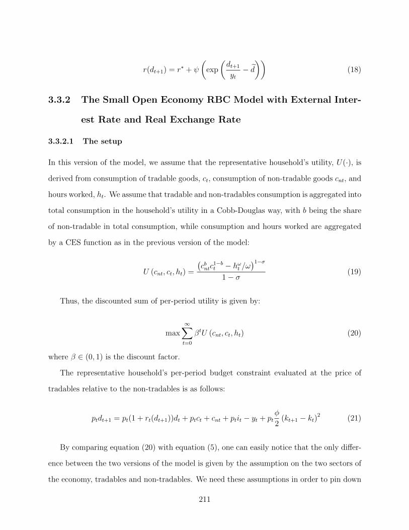
r(dt+1) = r∗ + ψ

(exp

(dt+1

yt− d))

(18)

3.3.2 The Small Open Economy RBC Model with External Inter-

est Rate and Real Exchange Rate

3.3.2.1 The setup

In this version of the model, we assume that the representative household’s utility, U(·), is

derived from consumption of tradable goods, ct, consumption of non-tradable goods cnt, and

hours worked, ht. We assume that tradable and non-tradables consumption is aggregated into

total consumption in the household’s utility in a Cobb-Douglas way, with b being the share

of non-tradable in total consumption, while consumption and hours worked are aggregated

by a CES function as in the previous version of the model:

U (cnt, ct, ht) =

(cbntc

1−bt − hωt /ω

)1−σ

1− σ(19)

Thus, the discounted sum of per-period utility is given by:

max∞∑t=0

βtU (cnt, ct, ht) (20)

where β ∈ (0, 1) is the discount factor.

The representative household’s per-period budget constraint evaluated at the price of

tradables relative to the non-tradables is as follows:

ptdt+1 = pt(1 + rt(dt+1))dt + ptct + cnt + ptit − yt + ptφ

2(kt+1 − kt)2 (21)

By comparing equation (20) with equation (5), one can easily notice that the only differ-

ence between the two versions of the model is given by the assumption on the two sectors of

the economy, tradables and non-tradables. We need these assumptions in order to pin down

211

the equilibrium path of the real exchange rate defined as the price of tradables relative to

non-tradables5.

The total output in this economy is given by the sum of the output produced by the two

sectors of the economy:

yt = Nt + ptTt (22)

We assume that the nature of the technology in the tradable sector is Cobb-Douglas, and

this sector uses capital and labor to produce output Tt:

Tt = kαt h1−αt (23)

Moreover, we assume that the production in the non-tradable sector is based on an

endowment which is fixed6 over time to N :

Nt = N (24)

3.3.2.2 Non-linear equilibrium conditions

The representative household maximizes lifetime utility (20) subject to the budget constraint

in (21), and chooses the optimal path of c nt, ct, ht, it, yt, kt+1, dt+1, λt∞t=0. Thus, the

following system of nonlinear equations describe the optimal dynamics of the model variables

c nt, ct, ht, it, yt, kt+1, dt+1, λt, pt, rt∞t=0:

(cbntc

1−bt − hωt /ω

)−σbcb−1nt c

1−bt = λt (25)

(cbntc

1−bt − hωt /ω

)−σ(1− b) cbntc−bt = λtpt (26)

5Based on this definition of the relative price, the real exchange rate is defined as the price of one unitof foreign currency in terms of domestic currency. Thus, an increase in the relative price (i.e. real exchangerate) captures a real depreciation of the domestic currency relative to the foreign currency.

6One can generalize this assumption by making assumptions about the nature of the technology, the typeof the inputs used etc. This generalization would not affect the conclusions that we draw in this paper.

212

(cbntc

1−bt − hωt /ω

)−σhω−1t = λtpt(1− α) kαt h

−αt (27)

λtpt = βλt+1pt+1 [1 + r(dt+1)] (28)

λtpt [1 + φ (kt+1 − kt)] = βλt+1pt+1

[1− δ + φ (kt+2 − kt+1) + α

(kt+1

ht+1

)α−1]

(29)

ptdt+1 = pt(1 + rt(dt+1))dt + ptct + cn,t + ptit − yt + ptφ

2(kt+1 − kt)2 (30)

yt = N + ptkαt h

1−αt (31)

kt+1 = (1− δ) kt + it (32)

r(dt+1) = r∗ + ψ

(exp

(dt+1

yt− d))

(33)

cnt = N (34)

3.4 Calibration

In order to solve the system of difference equations that characterize the optimal decision of

the small open economy in the two versions of the RBC model considered in the previous

section, we have to assign values to the model parameters. In this section we describe the

way we calibrate these parameters which we group in two categories: financial parameters

such as the elasticity of country spread and other model parameters.

213

3.4.1 The Elasticity of Country Spread with Respect to the Debt

to GDP Ratio

The elasticity of country spread with respect to the debt to GDP ratio of the small open

economy, ψ, plays an important role in understanding the channels through which the small

open economy adjusts externally. As the size of this parameter determines the size of the

country spread for a given gap between the actual and steady state debt to GDP ratio, it

has implications for the importance of the financial channel relative to the trade channel.

The small open economy real business cycle literature focusing on emerging economies

has been traditionally calibrating this parameter to the value 0.001. This calibration was

first introduced by Mendoza (1991) that studied real business cycle fluctuations in the case

of the Canadian economy. This calibration quantitatively implies a country spread which is

close to zero. As we show in Table 1, a 0.1 increase in the debt to GDP ratio relative to

the steady state induces only one basis point increase in the country spread. The cost of

borrowing of the small open economy is about the same as the world interest rate, exogenous

to the small open economy, under this calibration.Thus, we expect that none or only a tiny

fraction of the overall external adjustment is through the financial channel. We label this

case as the ”No financial adjustment” case as outlined in the third column of Table 1.

Table 1. Calibration of the elasticity of country spread w.r.t. the debt to GDP ratio (ψ)

Value of Type of adjustment Implied adjustment

ψ Source in the model in spread (bp)

0.001 Mendoza (1991) No financial adjustment 1

0.07 Rowland and Torres (2004) Financial adjustment 70

1.3 Schmitt-Grohe and Uribe (2016) Financial adjustment 1300

The empirical literature which investigates the determinants of country spread (Can-

tor and Packer, 1996; Eichengreen and Mody, 1998; Hilscher; Rowland and Torres, 2004;

214

Nosbusch et al, 2010) has concluded that it is misleading to assume that country spread is

exogenous, by pointing out that there is not only a certain feedback relationship between the

country spread and the world interest rate, but the country spread also reacts to movements

in economic fundamentals such as the degree of the external indebtedness of the country. A

series of reduced form papers have shown recently that in the case of emerging economies

the elasticity of country spread with respect to fluctuations in the external debt position of

these countries is much larger. For instance, Rowland and Torres (2004) estimate, by using

panel data econometrics techniques, that an average increase of 0.1 in the debt to GDP

ratio implies a 70 basis point increase on average in the JP Morgan EMBI Global spread

in the case of a panel of sixteen emerging economies. Considering a larger set of emerging

economies, a panel of thirty-one countries, Hilscher et al. (2010) also document a similar

size of the elasticity of country spread: they estimate in a panel regression framework that a

0.1 increase in the debt to GDP ratio implies an increase of the country spread by about 50

basis points.

In addition to these reduced form findings, we also document in this paper that the

elasticity of country spread with respect to the debt to GDP ratio is much higher than

0.001. By using Bayesian estimation techniques, we estimate a small open economy real

business cycle model with endogenous country spread in the case of five Central and Eastern

215

European countries7. Table 2 contains the point estimates of the ψ parameter.

Table 2. Bayesian estimates of ψ based on a prior distribution gamma

with expected value 0.15 and standard deviation 0.05

Country Posterior Confidence Implied adjustment

mean interval in spread (bp)

Bulgaria 0.044 [0.013, 0.073] 44

Czech Republic 0.061 [0.023, 0.094] 61

Hungary 0.072 [0.029, 0.112] 72

Poland 0.077 [0.031, 0.124] 77

Romania 0.081 [0.032, 0.131] 81

Note: Confidence interval concerning the 90% probability region.

The posterior mean ranges between 0.04 and 0.08, suggesting that the size of elasticity of

country spread with respect to the debt to GDP ratio implied by the structure of the small

open economy RBC model and observables on output, consumption, investment and net

exports, is consistent with the reduced form findings. An increase in the debt to GDP ratio

by 0.1 induces about 70 basis point increase in the spread on average across the five countries

in the case for which we performed the estimation.

Thus, in line with the reduced form findings of the previous literature and the structural

estimates documented in this paper, we consider a case in which we calibrate the ψ parameter

to 0.07. As outlined in Table 1, we consider a third case in which we calibrate ψ to 1.3, a

value that is documented by Schmitt-Grohe and Uribe (2016) in the case of Argentina.

However, this large elasticity implies a 1300 basis point increase in the country spread for a

0.1 increase in the debt to GDP ratio.

7The model is similar in structure to the model outlined in this paper. Details on the model and theestimation are included in Section A.3 of the Appendix.

216

3.4.2 Other Parameters of the Model

We calibrate the other parameters of the models by closely following the calibration used

in the real business cycle literature on emerging economies as summarized in Table 3. We

calibrate the capital share of income (α) to the long-run average of the compensation of

labor input to value added ratio in emerging economies. The rate of depreciation of capital

(δ) is calibrated to 0.1.

The preference parameters are set as follows: the coefficient of relative risk aversion (σ)

defining the curvature of the utility function is set to 2, while the exponent of labor in the

utility function, ω, is set to 1.455. These are in line with Schmitt-Grohe and Uribe (2003),

Neumeyer and Perri (2005) and Garcia-Cicco et al. (2010).

Table 3. Calibration of the other model parameters

Parameter Comments Value

α Capital share of income 0.32

δ Capital depreciation 0.1

σ Relative risk aversion 2

ω Labor in the utility function 1.455

r∗ Steady state level of gross foreign real interest rate 0.01

d Countries’ long run external debt to GDP ratio 0.744

φ Capital adjustment cost parameter 8

b Share of non-tradable sector 0.7

N Endowment in the non-tradable sector 70

The steady state level of gross foreign real interest rate or risk free real interest rate (r∗) is

calibrated to 0.01 which implies a discount factor (β) equal to 0.99. d, the long run external

debt to GDP ratio, is set to 0.744 in line with Schmitt-Grohe and Uribe (2003) who argue

that this is consistent with the average of the net foreign asset to GDP ratio across emerging

217

economies. Following the same paper, we calibrate the capital adjustment cost parameter

(φ) to 8. The rationale behind this large value is twofold. On the one hand, adjusting capital

stock in emerging economies is costly given a series of capital market frictions that are not

present in developed economies. On the other hand, setting this parameter to a lower value

would imply that investment is too volatile relative to the data.

Finally, we assume that the non-tradable sector accounts for about 70% of the total

output of the small open economy setting in this way parameter b to 0.7. Moreover, we

assume that the endowment in the non-tradable sector is constant over time and we set it

to 70. This is a simplifying assumption which does not have implications for the conclusions

at which we arrive based on the simulation exercise in the next section.

3.5 The External Financial Adjustment of the Small

Open Economy

In this section we use the two small open economy real business cycle models outlined in

Section 3.3 to study how the financial and trade channels operate in an explicit intertemporal

model that pins down the equilibrium paths of real exchange rate and forecastable returns

on the net international investment position of the small open economy. Moreover, by using

the calibrations presented in the previous section, we simulate the non-linear model under

the assumption of perfect foresight to study how the two financial channels interact with the

trade channel and shed light on the mechanism through which these channels operate.

The findings of the simulation exercise are striking. First, we show that the financial

channel plays a more important role relative to the trade channel in the external adjustment

of the emerging countries when the country’s external spread is more sensitive to fluctuations

in the debt to GDP ratio relative to the steady state. This is mainly due to the positive

financial externality present in the model implied mechanism, the importance of which in-

creases with the debt elasticity of the spread. Second, we document that initial conditions

218

matter for the type of the channel through the country undergoes the external adjustment.

The results of the simulation exercise show that the larger the initial external debt position

of the country relative to steady state is, the more important the financial channel is. Third,

we show that the financial channel plays a more important role than the trade channel in

the long run. Finally, we show that the global results are different from the local ones: the

financial channel plays a smaller role in the log-linearized model. The following two sections

present the details and demonstrate these findings. First, we take the small open economy

RBC model augmented with endognous country spread and simulate it to study the impor-

tance of the real interest rate channel, as the only financial channel in this version of the

model, relative to the trade channel. Then, we simulate the second version of the model that

encompasses both the real interest rate and real exchange rate as financial channels.

3.5.1 The Role of the Real Interest Rate Channel

In order to study the relative importance of the trade and real interest rate channels in the

small open economy’s external adjustment process, we first perform simulations of the small

open economy real business cycle model augmented by endogenous country spread. Thus, in

this version of the model the real interest rate is the only channel of financial adjustment. We

calibrate the system of non-linear equations in (11) - (18). As we assume perfect foresight,

this exercise is nothing else than a deterministic simulation of the non-linear equilibrium

conditions by using numerical methods. Thus, we can study the global dynamics of the

simulated adjustment instead of the local one which was the case if we log-linearized the

system. We simulate the adjustment of the model economy back to the steady state from an

initial state in which all the model variables, except the capital stock and the external debt

position, are at their steady state value. We assume that initially the capital stock is by 10%

below its steady state, while the external debt position is by 10% above its steady state. We

perform the simulation in two cases. First we assume that the elasticity of country spread,

ψ, is low by calibrating it to 0.001. Then, we keep all the parameter values the same but we

219

increase the value of ψ to 0.07. The results of the simulation under the two calibrations of ψ

are summarized in Figure 1. These simulation results suggest a series of interesting findings.

First, the financial channel seems to play a much more important role than the trade

channel when the country spread is more sensitive to fluctuations in the debt to GDP ratio

relative to the steady state. By comparing the adjustment path of the external debt, the

country spread, the current account and the trade balance, we can easily notice that the

external adjustment takes place through a combination of the trade and real interest rate

channels. However, starting from period thirty the type of the adjustment becomes very

different across the two economies. In particular, the external adjustment of the economy

that has low elasticity of the spread (i.e. ψ calibrated to 0.001) is only through adjustment

in current account starting from period thirty. As the cost of borrowing is not sensitive to

the increase in external debt, the country over-borrows in order to build up capital stock and

all the external adjustment is through the trade channel. On the other hand, in the economy

with the larger elasticity of the spread most of the adjustment in the initial periods and all

of the adjustment on the long run is through the financial channel, i.e. the real interest

rate channel. As the country spread is sensitive to fluctuations in the external debt in this

economy, the country will pay down debt and build up capital stock by saving and running

trade surplus in the initial periods of the adjustment. But in period thirty, the economy

reaches the level of external debt and capital stock that is consistent with the steady state

level of trade balance and current account. Thus, starting from this period all the adjustment

is through the real interest rate channel. This difference in the importance of the financial

channel across economies with different values of ψ becomes even more striking when we

calibrate this parameter to 1.3. Appendix A.4.1. summarizes the simulation results which

suggest that essentially all the external adjustment is through the financial channel when the

country spread is extremely sensitive to fluctuations in the external debt position relative to

steady state.

Second, by examining the adjustment path of consumption per capita and utility, one

220

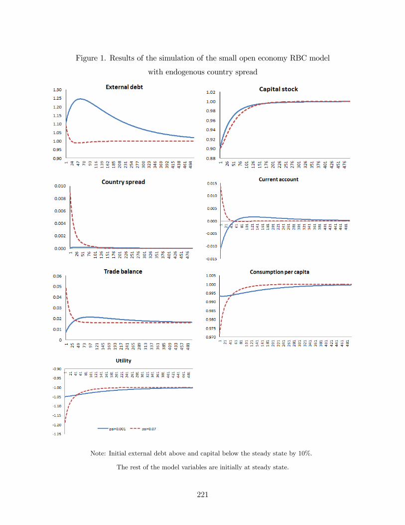
relative to steady state.

Figure 1. Results of the simulation of the small open economy RBC model

with endogenous country spread

Note: Initial external debt above and capital below the steady state by 10%.

The rest of the model variables are initially at steady state.

15

221

can notice that there seems to be a gain from the financial adjustment. This is because

the financial adjustment rewards countries for paying down debt. This is rationalized in the

model by the positive financial externality created by the endogenous country spread. Since

the spread depends on the deviation of the external debt to GDP ratio from its steady state,

building up capital stock and financing domestic consumption by building up new external

debt increases the cost of borrowing tomorrow and creates debt spiral over time. Moreover,

this increase in the cost of borrowing tomorrow is larger the larger the debt elasticity of

the spread. The small open economy internalizes the consequences of building up more

debt today as it makes per-period decisions by an optimal consumption-saving decision over

time. Thus, it will start the external adjustment by saving and paying down debt in the

initial periods that generates a positive financial externality over time, as the cost of external

borrowing falls over time. The more external debt is payed down, the larger the fall in the

cost of borrowing over time such that the spread adjusts back to a level at which the small

open economy can restart borrowing from the international markets.

The presence of the positive financial externality in the model rationalizes the finding

that the importance of the financial channel increases with the size of the debt elasticity of

the spread. Moreover, by the presence of this financial externality, the financial channel has

also non-trivial implications for welfare. Table 4 contains the sum of discounted simulated

utilities under different calibrations of the debt elasticity of country spread8, and under the

assumption that the initial debt is above its steady state debt by 10%, while the initial

capital stock is below its steady state by 10%.

Table 4. The sum of discounted utilities and the elasticity of country spread

ψ 0.001 0.7 1.3

Life-time utility (U0) 103.02 104.05 123.4

8To compute this, we simulate the consumption and hours worked under different parametrizations of ψand compute the life-time utility as

∑∞t=0βU(ct, ht) with β equal to 0.99, the discount factor value implied

by the r∗ calibrated to 0.01.

222

It shows that the larger ψ is the larger the discounted sum of lifetime utility implied by

the model. This suggests that there is always a gain from financial adjustment because it

rewards countries over time for paying down debt.

However, the financial externality and, thus, the financial channel plays an important role

in the external adjustment of the small open economy if the country starts the adjustment

from an initial external debt position that is above the steady state. In order to illustrate

this, we do additional simulation exercises in which we fix the initial external debt position

at a level below the steady state by 0.1. Table 5 contains the sum of discounted simulated

utilities under different calibration of the debt elasticity of country spread and different

assumptions on the initial value of the external debt position and capital stock9. Essentially,

the difference in the level of life-time utilities across the economies with different ψ is given

by the positive financial externality that is quantitatively important when the intial external

debt is above its steady state. As Table 5 illustrates, the financial channel matters for the

utility ranking only when the country is a net debtor on the international financial markets.

When the initial debt is below the steady state (i.e. the initial external debt of the country

is less than the steady state value), then the discounted lifetime utility is at the same level

across the economies with and without IFA.

Table 5. The sum of discounted utilities and the elasticity of country spread

ψ 0.001 0.07

Initial capital and debt below steady state by 0.1 37.6 37.4

Initial capital and debt above steady state by 0.1 37.7 38.1

Initial capital above and debt below steady state by 0.1 36.5 36.1

Initial capital below and debt above steady state by 0.1 38.9 39.4

Finally, Figure 1 suggests that the financial channel plays a more important role in

9To compute this, we simulate the consumption and hours worked under different parametrizations of ψand compute the life-time utility as

∑∞t=0βU(ct, ht) with β equal to 0.99, the discount factor value implied

by the r∗ calibrated to 0.01.

223

the external adjustment on the long run: as the country pays down external debt in the

initial periods, it starts to enjoy the benefits of the financial externality on the long run and

adjusts almost exclusively through the real interest rate channel. Figure 1 also suggests very

different global results from the local ones which studies the patterns of financial adjustment

in the neighborhood of the steady state. The first striking finding with respect to this is

that the financial channel plays a small role in the log-linearized model. The second is that

the interesting initial non-linearity in the adjustment is ignored in the log-linearized model.

By looking at the adjustment path of the external debt position in the neighborhood of the

steady state (i.e. around period four hundred) one would ignore not only the initial over-

and under-shooting in the external debt position in the initial periods of the adjustment,

but also the presence of real interest rate as adjustment channel. This is mainly because the

country spread is close to zero for these values of the external debt.

3.5.2 The Relative Importance of the Real Exchange and Interest

Rate Channels

In order to study the relative importance of the trade, real interest rate and real exchange

rate channels in the external adjustment process of the emerging economies, we first perform

simulations of the small open economy RBC model augmented with endogenous spread,

tradable and non-tradable sectors. Thus, in this version of the model the real interest rate and

the real exchange are the channels of financial adjustment. We calibrate the system of non-

linear equations in (25) - (33). Similarly to the previous simulation, under the assumption of

perfect foresight, we solve the non-linear equilibrium conditions by using numerical methods.

Then, we simulate the model by assuming that the initial capital stock is by 10% below its

steady state, while the external debt position is by 10% above its steady state and the

elasticity of country spread, ψ, can take two values: 0.001 and 0.07.

The results of the simulation under the two calibration of ψ are summarized in Figure 2.

These simulation results suggest that the findings documented in the previous section based

224

on the simulation of the model with only real interest rate as financial channel are robust

to the introduction of real exchange rate as an additional source of international financial

adjustment. Thus, the financial channel seems to be more important on the long run, and

in particular when the country spread is more sensitive to fluctuations in the debt to GDP

ratio. The real exchange rate, defined as the relative price of tradables adjusts over time

back to steady state through a real appreciation. However, there is essentially no significant

difference in the adjustment path across the two economies except for the first few periods.

All these suggest that the main source of external adjustment is the real interest rate channel

in the emerging economies that are characterized by debt elastic country spread.

The importance of the financial channel increases with the size of the debt elasticity of

the spread also when real exchange rate as IFA channel is present in the model in addition

to the country spread (i.e., the only channel of adjustment in the baseline verison of the

model considered in the previous section). Table 6 contains the sum of discounted simulated

utilities under different calibrations of the debt elasticity of country spread10, and under

the assumption that the initial debt is above its steady state debt by 10%, while the initial

capital stock is below its steady state by 10%.

Table 6. The sum of discounted utilities and the elasticity of country spread

ψ 0.001 0.7

Life-time utility (U0) 96.12 97.11

The two columns of Table 6 show that the larger ψ is the larger the discounted sum of

lifetime utility implied by the model. This suggests that there is always a gain from financial

adjustment because it rewards countries over time for paying down debt.

10To compute this, we simulate the consumption and hours worked under different parametrizations of ψand compute the life-time utility as

∑∞t=0βU(ct, ht) with β equal to 0.99, the discount factor value implied

by the r∗ calibrated to 0.01.

225

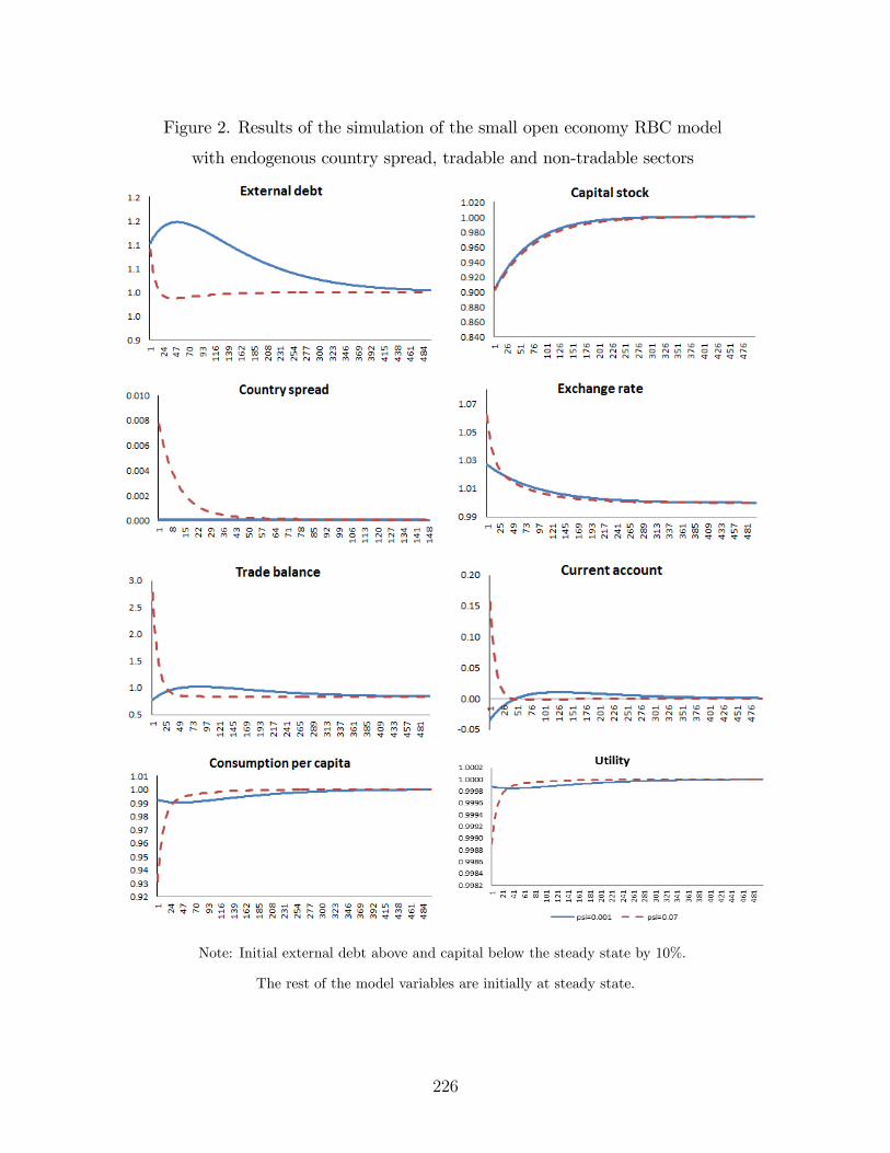
in the emerging economies that are characterized by debt elastic country spread.

Figure 2. Results of the simulation of the small open economy RBC model

with endogenous country spread, tradable and non-tradable sectors

Note: Initial external debt above and capital below the steady state by 10%.

The rest of the model variables are initially at steady state.

19

226

3.6 Conclusions

In this paper we have calibrated and demonstrated the importance of IFA in a standard open

economy growth model (Schmitt-Grohe and Uribe (2003)) with a well-defined steady level

of foreign liabilities. In this model there is a country specific credit spread which varies as a

function of the ratio of foreign liabilities to GDP. We studied a perfect foreign version of the

model so that we could characterize the global dynamic adjustment in net foreign assets, the

endogenous cost of debt service, and the path of the real exchange rate. This is important,

because in this model, in a neighborhood of the steady state, IFA is not very important.

In our baseline simulation in which we calibrate the elasticity of the country credit spread

to the debt to GDP ratio based on plausible empirical estimates from the literature as well as

our own estimates, we find that allowing for an IFA channel results in a very rapid converge

of the current account to its steady state (relative to the no IFA case) so that most of

the time that the country is adjusting , all the adjustment is via forecastable changes in the

costs of servicing debt and in the appreciation real exchange rate and none of the adjustment

is in the current account. By contrast, in the no IFA case, current account adjustment by

construction does all the work and current account adjustment calibrated to be much slower.

Finally we show that IFA adjustment via the real exchange rate can be important even if

forecastable changes in the cost of debt service are not. We discussed above, in this textbook

model there is a negative externality to foreign borrowing in that no borrower internalizes

that the credit spread faced by borrowers in the country are a function of aggregate debt.

We were able quantify that not only is IFA important in this model, lifetime utility in the

model with IFA is higher than in the model without even though – really because – the cost

of debt service is higher period by period until convergence is achieved.

227

A.1 Derivation of the BoP Accounting Identity with Zero Gross

International Asset Position

We aim to derive the log-linearized balance of payment accounting identity in the special

case when the gross international asset position of the country is zero in any time period,

i.e. At+1 = At = 0.

The BoP accounting identity in levels is:

At+1 − Lt+1

At − Lt= Rt+1

(1 +

Xt −Mt

At − Lt

)(A.1)

where At is the gross international asset position, Lt is the gross international liability

position, Rt is the real interest rate, Xt is total exports and Mt is total imports.

The assumption At+1 = At = 0 implies that A.1 can be written as:

Lt+1

Lt= Rt+1

(1− Xt −Mt

Lt

)(A.2)

While the steady state value of the gross asset position is zero, i.e. A = 0.

In the following, we want to show that the log-linearized version of the identity in A.2 is:

lt = nxt − ρnxt + ρlt+1 − ρrt+1 (A.3)

where lt is the log-deviation of the gross liability position from its steady state, nxt is the

log-deviation of net exports, defined as Xt−Mt from its steady state, rt+1 is the log deviation

of the real interest rate from its steady state, ρ ≡ 1 − X−ML

with X, M and L being the

steady state values of exports, imports and gross liability position.

By iterating forward on A.3 we get the intertemporal balance of payment identity that

pins down the current level of gross liability as the function of the discounted sum of future

228

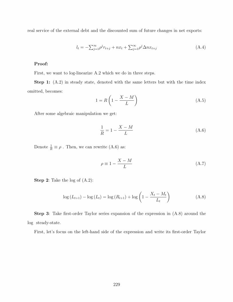
real service of the external debt and the discounted sum of future changes in net exports:

lt = −∑∞

j=1ρjrt+j + nxt +

∑∞j=1ρ

j∆nxt+j (A.4)

Proof:

First, we want to log-linearize A.2 which we do in three steps.

Step 1: (A.2) in steady state, denoted with the same letters but with the time index

omitted, becomes:

1 = R

(1− X −M

L

)(A.5)

After some algebraic manipulation we get:

1

R= 1− X −M

L(A.6)

Denote 1R≡ ρ . Then, we can rewrite (A.6) as:

ρ ≡ 1− X −ML

(A.7)

Step 2: Take the log of (A.2):

log (Lt+1)− log (Lt) = log (Rt+1) + log

(1− Xt −Mt

Lt

)(A.8)

Step 3: Take first-order Taylor series expansion of the expression in (A.8) around the

log steady-state.

First, let’s focus on the left-hand side of the expression and write its first-order Taylor

229

series expansion as:

log (Lt+1)− log (Lt) = log(elog(Lt+1))− log(elog(Lt)) ' (A.9)

' log (L)− log (L) +1

elog(L)elog(L)(log (Lt+1)− log (L))−

− 1

elog(L)elog(L)(log (Lt)− log (L))

= (log (Lt+1)− log (L))− (log (Lt)− log (L))

Denote the deviation of the variable from the log steady state as xt = log (Xt)− log (X) .

Then, (A.9) can be written as:

log (Lt+1)− log (Lt) ' lt+1 − lt

Second, we take the first-order Taylor series expansion of the right-hand side of (A.8)

around the steady state:

230

log (Rt+1) + log

(1− Xt −Mt

Lt

)= log

(elog(Rt+1)

)+ log

(1− elog(NXt)

elog(Lt)

)' (A.10)

' 1

elog(R)elog(R) (log(Rt+1)− log(R)) +

+1

1− elog(NX)

elog(L)

(−e

log(NX)

elog(L)

)(log(NXt)− log(NX)) +

+1

1− elog(NX)

elog(L)

(−−elog(NX)

(elog(L)

)(elog(L))

2

)(log(Lt)− log(L))

= (log(Rt+1)− log(R)) +

+NX

NX − L(log(NXt)− log(NX)) +

− NX

NX − L(log(Lt)− log(L))

= (log(Rt+1)− log(R))

+NX

NX − L[(log(NXt)− log(NX))− (log(Lt)− log(L))]

(1)

By using the notation in the case of log deviations, (A.10) becomes:

log (Rt+1) + log

(1− Xt −Mt

Lt

)' rt+1 +

NX

NX − L[nxt − lt]

By using expression (A.7) derived in the steady state, we can rewrite NXNX−L as:

NX

NX − L=

X −MX −M − L

=X −M − L+ L

X −M − L= 1 +

L

X −M − L(A.11)

= 1 +1

X−ML− 1

= 1− 1

1− X−ML

=

= 1− 1

ρ

231

Thus, the log-linearized version of equation (A.2) is:

lt+1 − lt = rt+1 +

(1− 1

ρ

)[nxt − lt] (A.12)

By rearranging A.12 we get:

lt = nxt − ρnxt + ρlt+1 − ρrt+1 (A.13)

One can easily notice that the expression in A.13 is exactly the expression in A.3 that

we wanted to show.

Next, we want to show that A.4 holds in this framework. By iterating forward on (A.13)

we get:

lt+1 = nxt+1 − ρnxt+1 + ρlt+2 − ρrt+2 (A.14)

Use (A.14) and plug it into (A.13):

lt = nxt − ρnxt + ρ (nxt+1 − ρnxt+1 + ρlt+2 − ρrt+2)− ρrt+2 (A.15)

= nxt + ρ(nxt+1 − nxt)− ρ2nxt+1 + ρ2lt+2 − ρrt+1 − ρ2rt+2

= nxt + ρ∆nxt+1 −∑2

j=1ρjrt+j + ρ2lt+2 − ρ2nxt+1

Similarly, by iterating n-steps ahead and plugging the iterated expression back into (A.15)

we get:

lt − nxt =∑n

j=1ρj∆nx

t+j−∑n

j=1ρjrt+j + ρnlt+n+1 − ρnnxt+n (A.16)

By using the transversality condition on the gross liability position:

limn→∞

E [ρnlt+n+1] = 0 (A.17)

and taking expression (A.16) in expectation conditional on information available at time t,

232

we get the expression:

nxt − lt =∑∞

j=1ρj(rt+j −∆nx

t+j

)(A.18)

By re-arranging terms, (A.18) can be written as:

lt = −∑∞

j=1ρjrt+j + nxt +

∑∞j=1ρ

j∆nxt+j (A.19)

But this is exactly the identity that we have in (A.4). Thus, we just proved that the

current gross liability position can be written as the expression in A.4.

A.2 Estimation Appendix

The bayesian estimates of the model parameters included in Table 2 are obtained by

structurally estimating a full scale small open economy RBC model by using Bayesian tech-

niques. This model is consistent with the small open economy model with endogenous

country spread considered in Section 3.3. Here we augment this model with a working capi-

tal constraint. This appendix is organized as follows. First, we outline the model. Then we

present the estimation strategy we use to parameterize the model.

A.2.1 Model Specification

A.2.1.1 Households’ behavior

The representative household chooses the sequence of values for Ct, ht, It, Kt+1, Dt+1, ∞t=0

in order to maximize the expected discounted sum of lifetime utility derived from the con-

sumption of goods and leisure:

maxCt,ht,Kt+1,Dt+1∞t=0

E0

∞∑t=0

βtU (Ct, ht,Γt−1) (B.1)

where Ct is time t consumption, ht labor supplied by the household at time t, β is the discount

factor, Γt−1 allows for balanced growth path in utility11, U() is twice differentiable concave

11More details about the way balanced growth path is defined you can find in the next subsection.

233

utility function, increasing in its first argument and decreasing in its second argument.

The household acquires income by supplying labor, ht to the firms and getting the wage,

wt in exchange, by renting capital, Kt to the firms at the rental rate of capital ut, and by

borrowing from, Dt+1 > 0 or by investing, Dt+1 < 0 in one period noncontingent bonds on

the international financial market. Thus, one unit of foreign asset or debt costs qt in units

of consumption goods. The household uses this income to purchase consumption goods, Ct,

to invest in investment goods, It and to pay back previous loans, Dt > 0, contracted from

or to sell international bonds, Dt < 0, purchased from these markets. In this way she

accumulates two types of capital stock which she owns entirely: physical capital, Kt and

internationally traded noncontingent bond, Dt. Thus, the household’s per period budget

constraint is:

wtht + utKt + qtDt+1 = Dt + Ct + It (B.2)

where the left-hand side of the identity characterizes the structure of the per period income,

while the right-hand side represent the per period expenditures.

Changing the capital stock is costly and in each period t it is realized according to a

capital accumulation rule which states that the per period capital stock is nothing else than

the sum of the existing capital stock net of depreciation, plus current investments minus the

adjustment cost, Φ (Kt+1, Kt) , paid for each unit of capital accumulated:

Kt+1 = (1− δ)Kt + It − Φ (Kt+1, Kt)Kt (B.3)

This modeling technique is frequently used in the RBC literature because it improves the

performances of the model to generate moderate investment volatility and increases the

persistence of investment. By assumption, Φ() is a strictly increasing, concave function.

A.2.1.2 Firms’ behavior

The representative firm behaves in a perfectly competitive way, hires labor, ht and rents

capital, kt in order to produce consumption goods, Yt based on a neoclassical production

234

technology, F ():

Yt = atF (Kt,Γtht) (B.4)

where at models transitory technology improvement defined as an exogenous autoregressive

stationary, |ρa| < 1, process of order one:

log at = ρa log at−1 + εat (B.5)

which captures shocks to total factor productivity as one source of uncertainty through

εat , i.i.d. process with mean zero and standard deviation σa. Γt models permanent technology

improvements as a labor augmenting productivity growth. As Aguiar and Gopinath (2007a)

showed, assuming stochastic trend improvement, the neoclassical growth model does better

job in replicating emerging market business cycle stylized facts like the countercyclical nature

of trade balance to output ratio or higher volatility of consumption than output. The main

intuition is related to the fact that as a result of a positive permanent productivity shock,

labor productivity increases permanently. This generates a larger increase in permanent

income and consumption than in current income which is financed by issuing external debt.

In line with Aguiar and Gopinath (2007a), we assume that permanent technology shocks act

through an exogenous and mean reverting stationary process:

Γt = gtΓt−1 (B.6)

log (gt/µ) = ρg log (gt−1/µ) + εgt

where |ρg| < 1, εgt is an i.i.d. process with mean zero and standard deviation σg, and it

models shocks to labor productivity which are incorporated into Γt through gt, resulting in

trend growth improvements. µ represents long-run labor productivity growth.

The representative firm has the primary objective to maximize the total discounted sum

235

of all future profits, Πt, subject to a working capital constraint:

maxat,ht,kt∞t+0

E0

∞∑t=0

βtΠt = E0

∞∑t=0

βtatF (Kt,Γtht)− wtht

[1 + θ

(Rt−1 − 1

)]− utKt

(B.7)

In other words, the working capital constraint induces an additional friction into the

model since the representative firm must borrow at Rt−1 rate of interest from the represen-

tative household in each period in order to be able to finance θ fraction of the wage bill at

the beginning of each period, in advance of the realization of the income. Neumeyer and

Perri (2005) and Uribe and Yue (2006) argue that this financial friction creates a linkage be-

tween interest rate movements and real economic activity, which improves the ability of the

baseline RBC model to generate strong countercyclical trade balance through the following

mechanism: falling interest rate, on the one hand, reduces the cost of labor allowing firms to

hire more labor and consequently to produce more output. On the other hand, the lower the

cost of borrowing boosts aggregate demand which generates deterioration in trade balance.

Thus output and trade balance move in the opposite direction when the cost of financing

changes through borrowing.

A.2.2 Closing the Model

A.2.2.1 The cost of borrowing

In order to solve the model a few more assumptions are needed concerning the dynamics

of domestic and world interest rates, country spread, the price of the foreign debt, and the

functional forms of the utility, production and capital adjustment cost function.

We assume that the domestic interest rate at which households lend to firms is defined

as the product of gross country spread, St, and gross foreign interest rate, R∗t :

Rt = StR∗t (B.8)

The dynamics of world interest rate is described by a mean reverting stationary, |ρr∗| <

236

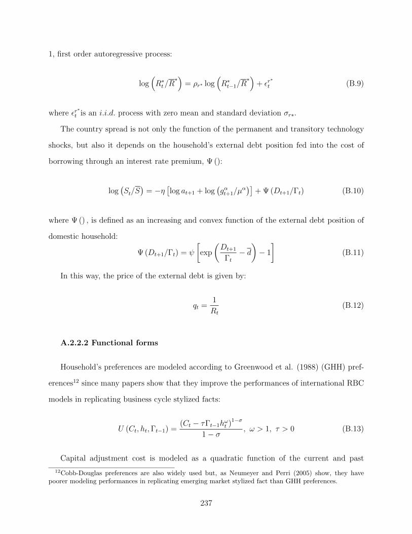
1, first order autoregressive process:

log(R∗t /R

∗)

= ρr∗ log(R∗t−1/R

∗)

+ εr∗

t (B.9)

where εr∗t is an i.i.d. process with zero mean and standard deviation σr∗.

The country spread is not only the function of the permanent and transitory technology

shocks, but also it depends on the household’s external debt position fed into the cost of

borrowing through an interest rate premium, Ψ ():

log(St/S

)= −η

[log at+1 + log

(gαt+1/µ

α)]

+ Ψ (Dt+1/Γt) (B.10)

where Ψ () , is defined as an increasing and convex function of the external debt position of

domestic household:

Ψ (Dt+1/Γt) = ψ

[exp

(Dt+1

Γt− d)− 1

](B.11)

In this way, the price of the external debt is given by:

qt =1

Rt

(B.12)

A.2.2.2 Functional forms

Household’s preferences are modeled according to Greenwood et al. (1988) (GHH) pref-

erences12 since many papers show that they improve the performances of international RBC

models in replicating business cycle stylized facts:

U (Ct, ht,Γt−1) =(Ct − τΓt−1h

ωt )1−σ

1− σ, ω > 1, τ > 0 (B.13)

Capital adjustment cost is modeled as a quadratic function of the current and past

12Cobb-Douglas preferences are also widely used but, as Neumeyer and Perri (2005) show, they havepoorer modeling performances in replicating emerging market stylized fact than GHH preferences.

237

capital stock level and it captures the fact that faster adjustments in the capital stock are

more expensive:

Φ (Kt+1, Kt) =φ

2

(Kt+1

Kt

− µ)2

(B.14)

The production function is assumed to be Cobb-Douglas, where Γt allows for labor aug-

menting productivity growth and α represents the share of labor in total income:

F (Kt,Γtht) = K1−αt (Γtht)

α (B.15)

Finally, the trade balance to output ratio is defined as:

TBYt =Yt − Ct − It

Yt(B.16)

In order to get the model to the data, a log-linear solution to the stationarized version of

the model has to be derived. Therefore we proceed in the following way: (1) we stationarize

the model by detrending all the variables which exhibit long run growth (2) then we derive

the first order conditions, which characterize the optimal behavior of the two types of agents

in the economy (3) finally, we log-linearize the optimality conditions around the steady state

of the model. The resulting linear rational expectation system of difference equations which

fully characterizes the optimal dynamics of the state and control variables was solved in

Matlab.

A.2.3 Calibration and Estimation

In order to solve the linear rational expectation system of difference equations, which fully

characterizes the optimal dynamics of the model economy, values to the model parameters

must be assigned. We do this in two different ways: we estimate, by using Bayesian tech-

niques, a set of parameters which are considered in the literature as being country specific

or difficult to calibrate, and we calibrate the rest of the parameters.

238

country:

Bulgaria The Czech Republic Hungary Poland Romania

J 0.6742 0.6012 0.6097 0.6820 0.6428

N 0.025 0.025 0.025 0.025 0.025

a 2 2 2 2 2

b s.t. h s.t. h s.t. h s.t. h s.t. hg 1.6 1.6 1.6 1.6 1.6

K 0.98 0.98 0.98 0.98 0.98

W 1.0130 1.0106 1.0071 1.0110 1.0151

r ∗ 1.0039 1.0039 1.0039 1.0039 1.0039

d 0.4457 0.1703 0.7617 0.3545 0.3145

h 0.3877 0.4665 0.3912 0.3828 0.4385

Table C.1. Calibrated Model Parameters

The labor share of income, ; is set at the ten years average of the compensation of labor

input to value added ratio in the case of each country. The rate of capital depreciation,

; is 0.025, which would imply a 10% annual depreciation rate and which is commonly used

in emerging market business cycles papers. The preference parameters are set as follows:

the coe¢ cient of relative risk aversion, ; dening the curvature of the utility function is

2; !; the exponent of labor in the utility function is 1.6 and the weight of labor in the per

period utility, ; is set such that it implies that households allocate h share of their total

time to working. These denitions and parameterizations are in line with those assumed by

Schmidt-Grohe and Uribe (2003), Neumeyer and Perri (2005), Garcia-Cicco et al. (2010)

and others. discount factor is set at 0.98 which would imply a 2.04% quarterly risk free

real interest rate.

The long run productivity growth; ; is dened as average real GDP growth rate over

the period 2000-200915. The steady state level of gross foreign interest rate, r; is computed

as the quarterly average of the Euro Zone real interest rate over 2000-2009 period. d; the

long run external debt to GDP ratio, is proxied as the 1997-2007 average of the net foreign

asset to GDP ratio. The steady state share of labor, h; is dened as the ten years average

employment to total population ratio.

15This type of association between parameter and statistical denition is used by Aguiar and Gopinath(2007a) in the case of Argentina and than it was taken over by other papers, e.g. Aguiar and Gopinath(2007b), Chang and Fernandez (2009).

10

Table A.2.1. Calibrated Model Parameters

A.2.3.1 Calibrated parameters

We set the value of the calibrated parameters based on long averages provided by macroe-

conomic data in the case of each country13, or we set them to values commonly used in

emerging market business cycle literature. These are presented in Table A.2.1 for each

country.

The labor share of income, α, is set at the ten years average of the compensation of labor

input to value added ratio in the case of each country. The rate of capital depreciation,

δ, is 0.025, which would imply a 10% annual depreciation rate and which is commonly used

in emerging market business cycles papers. The preference parameters are set as follows:

the coefficient of relative risk aversion, σ, defining the curvature of the utility function is

2; ω, the exponent of labor in the utility function is 1.6 and the weight of labor in the per

period utility, τ, is set such that it implies that households allocate h share of their total

time to working. These definitions and parameterizations are in line with those assumed by

Schmidt-Grohe and Uribe (2003), Neumeyer and Perri (2005), Garcia-Cicco et al. (2010)

13The last section of this appendix presents the source of this data.

239

and others. β discount factor is set at 0.98 which would imply a 2.04% quarterly risk free

real interest rate.

The long run productivity growth, µ, is defined as average real GDP growth rate over

the period 2000-200914. The steady state level of gross foreign interest rate, r∗, is computed

as the quarterly average of the Euro Zone real interest rate over 2000-2009 period. d, the

long run external debt to GDP ratio, is proxied as the 1997-2007 average of the net foreign

asset to GDP ratio. The steady state share of labor, h, is defined as the ten years average

employment to total population ratio.

A.2.3.2 Estimated parameters

We use Bayesian techniques as proposed by Smets and Wouters (2003), Lubik and

Schorfheide (2005) and An and Schorfheide (2007) over the sample period 1995Q1:2009Q4

in order to estimate those parameters which are country specific (e.g. working capital pa-

rameter, capital adjustment cost coefficient) or difficult to calibrate (e.g. the persistence and

standard deviation of different shocks, the elasticity of country spread with respect to the

Solow residual). These authors argue that the main advantage of the Bayesian estimation

of DSGE models in comparison with moment or impulse response matching is that the pa-

rameters are seen as random variables, and a prior density which incorporate initial beliefs

and information about these parameters is specified together with a likelihood function for

the DSGE model. Based on these, the posterior mode of each parameter can be computed

and by using Bayes theorem to update initial beliefs, the conditional distribution of each

parameter (i.e. posterior distribution) is calculated given the observable variables (i.e. data)

and the model. An and Schorfheide (2007) point out that the main benefit of this pos-

terior distribution consists of the fact that it permits to perform inference concerning the

parameters and to conduct a likelihood based checking of the goodness of fit.

14This type of association between parameter and statistical definition is used by Aguiar and Gopinath(2007a) in the case of Argentina and than it was taken over by other papers, e.g. Aguiar and Gopinath(2007b), Chang and Fernandez (2009).

240

Basically, this is a two step procedure: (1) in the first step the posterior mode is computed

by using an optimization routine to find that value of the parameters which minimizes the

negative log-likelihood given the model, the data based on which we perform the estimation

and prior probability distribution of the parameters to be estimated.15 The inverse of the

Hessian of the log-likelihood function is evaluated at the optimal posterior mode. (2) The

second step consists of running a Markov Chain Metropolis-Hastings (MCMH) algorithm

which constructs a Gaussian approximation around the posterior mode in the following way:

it draws a number from a normal distribution characterized by mean equal to the posterior

mode obtained in the previous step and variance-covariance matrix set at the inverse of the

log-likelihood function evaluated at the same posterior mode and scaled up by a constant

(i.e. jumping distribution). Then it decides whether to accept this newly drawn value as

the mean of the jumping distribution used for the next draw with a certain probability (i.e.

acceptance ratio computed as the ratio between the log-likelihood of the model evaluated

at the newly drawn parameter and the same likelihood evaluated at the parameter value

obtained from the previous draw) or to continue with the parameter value obtained from

the previous draw, with probability one minus the acceptance ratio. The more these draws

are repeated the more efficiently and effectively the algorithm can explore the posterior

distribution in the neighborhood of the posterior mode.

Therefore three main ingredients are needed to implement the above described proce-

dure: the model, the observable variables and the definition of the prior distribution of the

estimated parameters. Firstly, the model has to be written in a linear rational expectation

system form which is solved by using numerical methods.16 Then the model is written in

state space form together with the measurement equations while its likelihood is computed

by using the Kalman filter.

15To find the optimal value of the posterior mode we use a Monte-Carlo based optimization routine, with100000 simulations, implemented in Dynare. This turned out to be a more robust method than solving asimple constrained minimization problem.

16For this we use perturbation methods implemented in Dynare toolbox which provide as a solution alinear dynamic version of the model which contains the dynamics of the state and control variables, i.e.policy functions.

241

Secondly, the observable variables must be defined and fed into the model. We use four

observable variables because they are available in the case of all countries and the method-

ology based on which they are collected should not differ across countries. These are the

HP filtered quarterly gross domestic product (obsY ), consumption (obsC) and investment

(obsINV E) taken in logarithm and HP filtered trade balance to output ratio (obsTBY ) over

the period 1995:1-2009:4. We assume that these observables are subject to measurement er-

rors because of two reasons. One reason is technical in nature, and it aims to overcome

the stochastic singularity problem, i.e. the number of structural shocks in the model must

be equal to the number of observables considered for the estimation. Since in the present

models there are three, respectively four shocks, at least one measurement error must be

included while estimating the uniform interest rate and non-persistent country spread ver-

sion of the model or at least two measurement errors have to be defined when estimating

the uniform interest rate and persistent country spread extension. We assume that the

measurement errors εobsY , εobsC , εobsI , εobsTBY follow i.i.d. processes with zero mean and

σz2=εobsY ,εobsC ,εobsI ,εobsTBY standard deviation. The other reason for defining measurement

errors is related to the potential role they play in conducting robustness check of the re-

sults. Therefore, when estimating the model we distinguish two cases: estimation without

measurement errors, when we augment the state space just by as many measurement errors

as many are needed to overcome the stochastic singularity problem, versus estimation with

measurement errors, when we consider that all the observables contain measurement error.

By considering that macroeconomic data usually contain errors and omissions because of

aggregation, changes in methodologies, definitions, rules and regulations applied during col-

lecting them the inclusion of measurement errors should improve the estimation results if

the errors are indeed influential.

Finally, the prior distribution is usually subjective because it describes uncertainty and

prior knowledge about the model and its parameters. We select the shape of the distribution

based on those applied in earlier papers on emerging market business cycles and based on the

242

restrictions regarding possible domain of definition of different parameters. The expected

value and standard deviation of each distribution assumed are set at values provided by

macroeconomic data. Overall, we estimate eleven structural parameters, as reported in

Table 5 which can be divided into two groups.

Parameter Prior shape Expected value Std. dev.

σz1 Gamma 0.2 0.1

Inverse Gamma 0.2 Inf

ρa Beta 0.9 0.01

ρg Beta 0.72 0.01

ρr∗ Beta 0.8 0.01

η Gamma 0.5 0.1

ψ Gamma 0.15 0.05

φ Gamma 6 2

θ Beta 0.5 0.1

σz2 Gamma 0.02 0.01

Inverse Gamma 0.02 Inf

Table A.2.2 Prior Distribution of the Estimated Model Parameters

The first group contains the persistence and the standard deviation of the shock pro-

cesses. In line with previous studies, we assume that the persistence of the AR(1) shock

processes follow Beta distribution because this distribution is the most suitable for param-

eters taking values between zero and one. The standard deviation of this distribution is

harmonized across different shocks and it is set at 0.01 while the mean of the distribution

differs across shocks. Since the transitory technology shock is documented in the literature

as persistent (e.g. Smets and Wouters, 2007; Chang and Fernandez, 2009; Garcia-Cicco et

al., 2010), we set the mean of the distribution of ρa to 0.9; the mean of the persistence of

243

permanent technology shock, ρg, is set at 0.72 since previous estimation results reported in

the RBC literature suggests that it is less persistent than the transitory one; quantitative

macroeconomic literature provides a series of evidences that US and Euro Zone real interest

rates are both highly persistent or they follow an almost random walk process. Uribe and

Yue (2006) estimate an AR(1) process on the 3-month real gross Treasury bill rate and they

obtain a significant point estimate of the persistence parameterequal to 0.83. Similarly, Lu-

bik and Schorfheide (2005) estimate the same parameter and get 0.84 in the case of the US

and 0.83 in the Eurozone. Thus, we set the mean of the distribution of ρr∗ at 0.8 while the

distribution of the persistence of country spread is assumed to have mean 0.65 in line with

the autocorrelation coefficient of the EMBI spread reported in the first section of the paper.

The distribution of the standard deviation of the shock processes(σz1=εa,εg ,εr∗ ,εs

)is con-

sidered being the same across different types of shocks. Generally, in the quantitative macro

literature dealing with Bayesian estimation of DSGE models, standard errors of shocks are

assumed to follow inverse gamma distribution mainly because this is a sensible distribution

to relative shock sizes17. Moreover, gamma distribution could be another good candidate

for the distribution followed by these standard deviations because it is used in the case of

parameters which take positive values. Thus, we estimate each specification of the model

by considering two cases: first, we assume that the standard deviation of the shocks follows

gamma distribution with mean 0.2 and standard deviation 0.1, while, in the other case, we

consider inverse gamma distribution with mean 0.1 and scale parameter infinity.

The second group of structural parameters consists of those parameters which character-

ize financial decisions in the model. These are the elasticities of country spread with respect

to Euro Zone interest rate, ηr∗ , and Solow residual, ηSR. Since with the exception of ηSR in

the case of Argentina there are no previous evidences concerning the Bayesian estimation

of these parameter we assume that they follow Gamma distribution (i.e. they take positive

values because it is intuitive to assume that country spread increases as Euro Zone interest

17For a detailed description of the most frequently used distributions in DSGE Bayesian estimation, ad-vantages and shortcomings of them consult Ermolaev et al. (2008): Estimating GPM with Dynare mimeo.

244

rate gets higher or when a negative productivity shock hits the economy) with mean 0.5

and standard deviation 0.1. The mean of the distribution was set based on the observed

correlation coefficient between EMBI spread and Euro Zone interest rate, on the one hand,

and EMBI spread and output, on the other hand.

Another financial parameter of the model is the debt-elastic interest rate parameter,

ψ, which measures the sensitivity of interest rate/country spread to fluctuations in external

debt position. This parameter is usually not estimated and is calibrated at 0.001, value

which was proposed by Mendoza (1991) in the case of the Canadian economy. Garcia-Cicco

et al. (2010) are the only authors who estimate this parameter, assuming that it follows

uniform distribution. Thus it is worth to pay particular attention to this parameter and

estimate it because it could easily happen that in the case of emerging economies the data

would attribute a higher value to it. Logically it can be expected that country spread is more

sensitive to movements in debt position in emerging economies than in developed countries;

hence calibrating it to 0.001 would be erroneous. We assume that this parameter follows a

gamma distribution with mean 0.15 and standard deviation 0.05. This is a rather loose prior

but since there is no previous evidence on estimating it, the prior should take into account

this uncertainty (i.e. this is why the standard deviation of the distribution takes relatively

high value).

Because the capital adjustment cost parameter, φ, is a positive parameter it is assumed

to follow a gamma distribution with mean 6 and standard deviation 2.18 This is a some-

what tighter prior than those assumed by Chang and Fernandez (2009) who estimate φ by

considering that it follows a gamma (3,2) distribution in the case of Mexico or Smets and

Wouters (2007) who assume normal (1.25, 0.24) in the case of Eurozone. However, this is

in line with Garcia-Cicco et al. (2010) who consider gamma(8,4) distribution. The working

18We estimated the model by assuming a loose prior for the distribution of φ like gamma (3,2) for the firsttime and then we systematically tightened the prior by increasing the mean of the distribution. It turnedout that indifferently of how tight or loose the prior is the data and the model had the tendency to push upthe posterior mode of φ to values around 6 across all the countries. Hence we set the mean at 6 in order toobtain a better fit.

245

capital constraint, θ, parameter takes values between zero and one, thus we assume that it

follows Beta distribution with mean 0.5 and standard deviation 0.1. The main motivation

for setting the mean of this parameter to 0.5 is provided by the data which suggests that

the cross country average of the short run private credit of non-financial corporations to

value added ratio is around 0.45. This assumption is similar to those made by Chang and

Fernandez (2009).

Finally there is a set of nonstructural parameters which consists of the standard deviation

of measurement errors(σz2=εobsY ,εobsC ,εobsI ,εobsTBY

).We estimate the model by assuming that

these parameters follow: inverse gamma with mean 0.02 and scale parameter set to infinity or

gamma distribution with mean 0.02 and standard deviation 0.01. This is a wide prior, but in

this way uncertainty concerning the values of these standard deviations can be incorporated

into the prior knowledge.

We set the algorithm to make one hundred thousand draws19; the initial 50% of draws

were dropped out to ensure that the results do not depend on the initial value, and the

scaling parameter in the jumping distribution was fine tuned (around 0.4) such that to

obtain approximately one third acceptance ratio. Moreover, in order to conduct convergence

diagnostic (i.e. ensure that two different chains converge to the same stationary distribution)

we run two parallel Markov Chains and check the presence of convergence by comparing

recursively computed second order moments20 of the distributions constructed under each

and every draw per chain.

The estimation results can be summarized as follows: (1) The goodness of fit statistics

indicate that the specification which fits the best the data assumes gamma distribution

for the standard deviations of the shocks, all the observable variables contain measurement

19Initially, we set the number of draws to half a million in the MCMH algorithm but due to the robustnessof the optimization method used in the first step the two chains started to converge fast after 20000 draws.We checked if this convergence is present in the case of all the five countries by estimating the Chang andFernandez (2009) version of the model with both 100000 and half a million draws. The estimation resultsand the convergence statistics confirmed that 100000 draws are enough to achieve convergence.

20These second order moments are the variance of the distribution, skewness and confidence intervalconstructed around the parameter mean.

246

errors and the parameter ψ is estimated in the case of all the five sampled countries, (2) The

point estimates of ψ suggest that it is erroneous to calibrate the debt elastic interest rate

parameter to 0.001, as proposed by Mendoza (1991) and as it has been used so far in the

literature. The data suggests that, given the considered model setup, ψ varies in [0.02, 0.23]

interval across countries and across different model specifications, (3) The posterior means of

the persistence and standard deviation parameters of the shocks are relatively stable across

different model specifications, and (4) Financial parameters (like the elasticity of country

spread, working capital constraint or capital adjustment cost parameter) vary slightly across

different model versions. In addition, a certain degree of heterogeneity in the point estimates

of these financial parameters can be observed across countries. The rest of this subsection

discusses these results in more details.

When the debt elastic interest rate parameter, ψ, is not estimated, the estimates of

financial parameters21, especially that of the capital adjustment cost parameter changes

significantly, as reported in Table A.2.3. Independently of the model version considered, by

calibrating ψ to 0.001, as proposed by Mendoza (1991), the estimate of the capital adjustment

cost parameter becomes more than double in comparison with the case when ψ is estimated.

In addition, the elasticity of country spread and the working capital constraint parameter

increase.

ψ Bulgaria Czech Rep. Hungary Poland Romania

Calibrated to 0.001 17.29 13.14 13.62 14.22 14.68

Estimated 7.93 7.79 6.48 4.99 7.61

Table A.2.3. Posterior mean of φ under different specification of ψ

This result is not counterintuitive at all and it actually underlines the role of capital

adjustment cost in the model. When ψ is calibrated to a low value relative to what the

21For example, the elasticity of country spread with respect to the Solow residual and Euro Zone interestrate or the working capital constraint parameter.

247

data would imply the interest rate is less sensible to large movements in external debt, i.e.

external financing is relatively cheap. Consequently, agents would like to adjust even more

their capital stock by using besides their own funds more external financing, generating in

this way higher investment volatility. In order to limit this investment volatility, the cost of

an additional unit of capital accumulated must be higher, i.e. the capital adjustment cost

parameter must increase.

For example, Chang and Fernandez (2009) calibrate ψ instead of estimating it and they

obtain a point estimate of φ equal to 14.72 in the case of Argentina. This result is similar

to those we report in Table A.2.3 suggesting two digit numbers for φ across all the countries

when ψ is calibrated. However, when ψ is estimated its point estimates vary in [0.02, 0.23]

interval depending on country, model and prior specification. These are somewhat lower

estimates than the ψ equal to 2.8 reported by Garcia-Cicco et al. (2010). This indicates

that the data shifts the posterior mode of the conditional distribution upper, to the right

in the distribution of the parameter, suggesting that the external debt elasticity of country

spread or interest rate in the case of CEECs might be higher than 0.001, i.e. country spread

or interest rate is more sensitive to changes in the external debt position in CEECs than in

developed ones, like Canada.

Regarding the estimates of φ reported in Table A.2.3, one can observe that φ takes values

between 3.4 and 8.2 when ψ is estimated. These results are not at odds neither with the

previous evidences in RBC literature nor with the existing empirical evidences obtained

from research on investment behavior. For example Cummins et al. (2006) estimate φ by

using cross section data of firms from the US and conclude that the estimated φ is about 7.2

in the US. Thus, the estimates of φ obtained both in the case of the uniform interest rate

model and the persistent spread model are quite plausible. To motivate lower estimates of

φ, one can use the figures reported by Aguiar and Gopinath (2007a) who obtain estimates

for φ between 2.82 and 3.79 by using moment matching, or those recently documented by

Garcia-Cicco et al. (2010) (i.e. they estimate φ at 4.6 in the case of Argentina by using

248

Bayesian techniques).

A.3 Data Appendix

1. National account components from Eurostat (quarterly frequency): the following

components measured in millions of national currency chain-linked volumes (reference year

2000) are used in the paper (with the corresponding identification code in the brackets):

1.1. Output: gross domestic product at market prices (B1GM) series

1.2. Consumption: household and NPISH final consumption expenditure (P31 S14 S15):

1.3. Investment: gross fixed capital formation (P51)

1.4. Exports: exports of goods and services (P6)

1.5. Imports: imports of goods and services (P7)

1.6. Trade balance to output ratio: is the ratio between net exports, computed as the

difference between exports of goods and services (P6) and imports of goods and services

(P7), and gross domestic product at market prices (B1GM)

weseasonally adjusted of all the above presented series by using Tramo-Seats method

implemented in Demetra 2.1. software package.

Cyclical components (logarithmic deviation from the long run trend) of the seasonally

adjusted output, consumption investment and trade balance to GDP ratio: are computed

in three steps (i) firstly, the above described level series are taken in logarithm (ii) the time

series, obtained in this way, are filtered by using Hodrick-Prescott filter with λ=1600 scale

parameter (iii) the cyclical component of each series is computed as a difference between the

logged level series and its trend component.

2. Real Euro Zone interest rate (quarterly frequency): is computed as the difference

between the overnight German money market rate and annualized quarterly German inflation

rate. The source of the interest rate is the Online Historical Financial Statistics published

by The Deutsche Bundesbank and it is defined as Frankfurt banks / Overnight money /

Monthly average: SU0101, from which the quarterly series is constructed by taking the

249

corresponding monthly rate at the end of each quarter. The annualized quarter-to-quarter

inflation rate is computed based on the quarterly consumer price index (13464ZF)(2000=100)

from International Financial Statistics of IMF according to the following formula:

inf = 400 ∗ ln

(CPIt,2000=100

CPIt−1,2000=100

)(20)

3. Country spread (quarterly frequency): is quantified by using JP Morgan EMBI Global

Divers-Stripped spread in Poland (JPMGPOC (SSPRD)) covering the period 1995Q1:2009Q4,

in Hungary (JPMGHNC (SSPRD)) over the period 1999Q1:2009Q4 and in Bulgaria (JPMP-

BUL (BSPRD)), 1994Q3:2009Q4; In order to compute EMBI spread US-dollar denominated

Brady bonds, Eurobonds, and traded loans issued or guaranteed by sovereign entities are

considered. Only issues with a current face amount outstanding of $500 million or more and

a remaining life of greater than 2 1/2 years are eligible for inclusion in the index. 22 Moreover

the yield spread used in the case of Hungary is computed as the absolute difference between

yield on long term Eurobonds issued by the Hungarian government (568915(RYAN)) and

yield on long term US Treasury bonds. (993766(RYAN)) 23.

4. Compensation of labor input (annual frequency): (i) total compensation of labor

(lab tot) is obtained from the EU KLEMS database for The Czech Republic, Poland and

Romania. This is computed as the sum of compensation for employees and that part of

the operating surplus/ mixed income which represents the compensation for self-employed

24 Data concerning mixed income is not available in the case of Bulgaria and Romania (ii)

compensation of employees at industry level published by Eurostat in the National Accounts

by 6 branches at current prices (nama nace06 c) and defined as the total remuneration, in

cash or in kind, payable by an employer to an employee in return for work done by the latter.

Social contributions paid by the employer are also included in this indicator.

22Source: http://www.jpmorgan.com/pages/jpmorgan/investbk/solutions/research/EMBI23Source: Datastream24For more details see EU KLEMS Growth and Productivity Accounts Version 1.0 Methodology, March

2007 http://www.euklems.net/

250

5. Value added (annual frequency): (i) total value added in the economy (all industries)

at current prices, in millions of euro, is obtained from the EU KLEMS database (va tot) for

Hungary, the Czech Republic and Poland; in the case of Bulgaria and Romania the source

of value added is Eurostat (B1G) (ii) industry level value added series, at current prices, in

millions of national currency, are from the National Accounts aggregates and employment

by branch tables (NACE) (nama nace) published by Eurostat.

6. Private credit of non-financial corporations (annual frequency): since there are no

publicly available figures concerning the type of loans besides their maturity for the Czech

Republic, Hungary and Romania, short term financial liabilities (stocks) of non-financial

corporations in millions of national currency, from the Czech National Bank’s, the National

Bank’s of Hungary and the Romanian National Bank’s Monetary and financial statistics,

are taken as proxy for working capital loans; working capital loans to non-financial private

corporations (stocks) in millions of national currency is considered in the case of Poland

published by the National Bank of Poland in the Monetary and financial statistics: Assets

and liabilities of monetary financial institutions; Bulgaria: there is no publicly available data.

7. Real GDP growth rate (quarterly frequency): measured as the percentage change of

the gross domestic product at constant prices relative to the previous period from the GDP

and main components-volumes (namq gdp k) table published by Eurostat

8. Net Foreign Asset (NFA) position (annual frequency): in millions of US dollars is from

the updated and extended version of dataset constructed by Lane and Milesi-Ferretti (2007)

in the ”External Wealth of Nations” Dataset, 1970-2007

9. Gross Domestic Product (annual frequency): is at current prices, in millions of US

dollars from the updated and extended version of dataset constructed by Lane and Milesi-

Ferretti (2007) in the ”External Wealth of Nations” Dataset, 1970-200725

10. Employment: (annual frequency): measured as annual average total employment (15-

64 years, resident population concept - LFS) in thousand of persons from the Employment

25More details about the source of the data at http://www.philiplane.org/EWN.html

251

(main characteristics and rates) (lfsi emp a ) table published by Eurostat.

11. Population: is in thousand of persons and it is obtained from Population, activity

and inactivity - Annual averages (lfsi act a) table, Eurostat.

252

A.4 Graphs

A.4.1. Results of the simulation of the small open economy RBC model with

endogenous country spread (initial external debt above and capital below their steady

stateby 10%)

D. Graphs and Tables

D.1. Results of the simulation of the small open economy RBC model withendogenous country spread (initial external debt above and capital below their steady

stateby 10%)

21253

Bibliography

[1] Acemoglu, D. and Guerrieri, V. (2008), ”Capital Deepening and Non-Balanced Eco-

nomic Growth”, Journal of Political Economy, 2008, 116 (3), 467-498.

[2] Acemoglu, D., Autor, D., Dorn, D., Hanson, G. and Price, B. (2016), “Import Compe-

tition and the Great U.S. Employment Sag of the 2000s”, Journal of Labor Economics,

34(S1), S141-S198.

[3] Aghion, P., Howitt, P. and Mayer-Foulkes, D. (2005), ”The Effect of Financial Devel-

opment on Convergence: Theory and Evidence,” The Quarterly Journal of Economics,

MIT Press, vol. 120(1), pp. 173-222.

[4] Aguiar, M. and Gopinath, G. (2007a), ”Emerging Market Business Cycles: The Cycle Is

the Trend”, Journal of Political Economy, University of Chicago Press, vol. 115, pages

69-102.

[5] Aguiar, M. and Gopinath, G. (2007b), ”The Role of Interest Rates and Productivity

Shocks in Emerging Market Fluctuations”, Working Papers Central Bank of Chile 445,

Central Bank of Chile.

[6] Ahn, J., Amiti, M., and Weinstein, D. (2011), “Trade Finance and the Great Trade

Collapse”, American Economic Review Papers and Proceedings, vol. 101(3), pp. 298-

302.

254

[7] Alessandria, G., Kaboski, J. and Midrigan, V. (2010), “The Great Trade Collapse of

2008-09: an Inventory Adjustment?“, NBER Working Paper . 15059

[8] Amiti, M. and Davis, D. (2012), ”Trade, Firms, and Wages: Theory and Evidence,”

Review of Economic Studies, Oxford University Press, 79(1),1-36.

[9] Amiti, M. and Freund, C. (2010), ”The Anatomy of China’s Export Growth,” NBER

Chapters, in: China’s Growing Role in World Trade”, NBER Working Paper.

[10] Amiti, M., Itskhoki, O. and Konings, J. (2014), ”Importers, Exporters, and Exchange

Rate Disconnect,” American Economic Review, 104(7), 1942-78.

[11] Amiti, M. and Khandelwal, A. (2013), ”Import Competition and Quality Upgrading”,

The Review of Economics and Statistics, MIT Press, 95(2), 476-490.

[12] Amiti, M. and Konings, J. (2007), ”Trade Liberalization, Intermediate Inputs, and

Productivity: Evidence from Indonesia”, American Economic Review, 1611-1638.

[13] Amiti, M. and Wei, S. (2006), ”Service Offshoring and Productivity: Evidence from the

United States”, NBER Working Papers 11926.

[14] Amiti, M., and Weinstein, D. (2011), “Exports and Financial Shocks”, The Quarterly

Journal of Economics, vol. 126(4), pp. 1841–1877.

[15] Amiti, M. and Weinstein, D. (2013), “How Much Do Bank Shocks Affect Investment?

Evidence from Matched Bank-Firm Loan Data, Federal Reserve Bank of New York Staff

Reports 604.

[16] An, S. and Schorfheide, F. (2005), ”Bayesian Analysis of DSGE Models”, CEPR Dis-

cussion Papers 5207, C.E.P.R. Discussion Papers.

[17] An, S. and Schorfheide, F. (2007), ”Bayesian Analysis of DSGE Models”, Econometric

Reviews, Taylor and Francis Journals, vol. 26(2-4), pages 113-172.

255

[18] Antras, P. and Helpman, E. (2004), ”Global Sourcing,” Journal of Political Economy,

112(3), 552-580.

[19] Antras, P. and Chor, D. (2013), “Organizing the Global Value Chain” , Econometrica,

81(6), 2127–2204.

[20] Antras, P. and Foley, F. (2011), Regional Trade Integration and Multinational Firm

Strategies in Costs and Benefits of Economic Integration in Asia, Robert J Barro and

Lee, Jong-Wha, Ch. 8. Oxford, New York: Oxford University Press.

[21] Antras, P., Fort, T. and Tintelnot, F. (2016), ”The Margins of Global Sourcing: Theory

and Evidence from U.S. Firms”, Working Paper.

[22] Arellano, C. and Mendoza, E. G. (2002), ”Credit Frictions and ’Sudden Stops’ in Small

Open Economies: An Equilibrium Business Cycle Framework for Emerging Markets

Crises”, NBER Working Papers 8880, National Bureau of Economic Research, Inc.

[23] Arellano, C. and Ramanarayanan, A. (2006) ”Default and the Term Structure in

Sovereign Bonds”, 2006 Meeting Papers 299, Society for Economic Dynamics.

[24] Arvai, Zs. (2005), ”Capital Account Liberalization, Capital Flow Patterns, and Policy

Responses in the EU’s New Member States”, IMF Working Paper, WP/05/213.

[25] Atalay, E., Hortacsu, A. and Syverson, C. (2013), ”Vertical Integration and Input

Flows”, American Economic Review, 104(4), 1120-48.

[26] Atkeson, A. and Burstein, A. (2010), ”Innovation, Firm Dynamics, and International

Trade,” Journal of Political Economy, 118(3), 433-484.

[27] Autor, D. and Dorn, D. (2013), ”The Growth of Low Skill Service Jobs and the Polar-

ization of the U.S. Labor Market”, American Economic Review, 103(5), 1553-1597

256

[28] Autor, D., Dorn, D. and Hanson, G. (2013), “The China Syndrome: Local Labor Mar-

ket Effects of Import Competition in the United States”, American Economic Review,

103(6), 2121-2168.

[29] Autor, D., Dorn, D. Hanson, G. and Song, J. (2014), ”Trade Adjustment: Worker Level

Evidence”, Quarterly Journal of Economics, 129(4), 1799-1860.

[30] Autor, D., Dorn, D. and Hanson, G. (2015), ”Untangling Trade and Technology: Evi-

dence from Local Labor Markets”, Economic Journal, 125(584), 621-646.

[31] Autor, D., Dorn, D. and Hanson, G. (2016), “The China Shock: Learning from Labor

Market Adjustment to Large Changes in Trade”, Annual Review of Economics (forth-

coming).

[32] Baily, M. and Bosworth, B. (2014), ”US Manufacturing: Understanding Its Past and

Its Potential Future”, Journal of Economic Perspectives, 28 (1), 3-26.

[33] Baldwin, R. and Robert-Nicoud, F. (2008), ”Offshoring: General Equilibrium Effects

on Wages, Production and Trade,” Development Working Papers 250.

[34] Baldwin, R. and Robert-Nicoud, F. (2014), ”Trade-in-goods and trade-in-tasks: An

integrating framework,” Journal of International Economics, 92(1), 51-62.

[35] Baldwin, R. and Venables, A. (2013), ”Spiders and snakes: Offshoring and agglomer-

ation in the global economy,” Journal of International Economics, Elsevier, vol. 90(2),

pp. 245-254.

[36] Bas, M. and Ledezma, I. (2010), ”Trade integration and within-plant productivity evo-

lution in Chile,” Post-Print hal-00562714, HAL.

[37] Bas, M. and Bombarda, P. (2013), ”Chinese trade reforms, market access and foreign

competition: the patterns of French exporters,” Policy Research Working Paper Series

6330.

257

[38] Blaum, J., Lelarge, C. and Peters, M. (2016), ”The Gains from Input Trade With

Heterogeneous Importers”, Working Paper.

[39] Bresnahan, T. and Levin, J. (2012), Vertical Integration and Market Structure, NBER

Working Paper 17889.

[40] Broda, C. and Weinstein, D. (2006), ”Globalization and the Gains From Variety,” The

Quarterly Journal of Economics, 121(2), 541-585.

[41] Bernard, A. and Jensen, B. (2007), “Firm Structure, Multinationals, and Manufacturing

Plant Deaths”, The Review of Economics and Statistics, 89 (3), 193-204.

[42] Bernard, A., Bradford, J., Redding, S. and Schott, P. (2011), Intra-Firm Trade and

Product Contractibility, American Economic Review, 100(2).

[43] Bernard, A. and Fort, T. (2015), “Factoryless Goods Producing Firms”, American

Economic Review Papers and Proceedings, 105(5).

[44] Bernard, A., Smeets, V. and Warzynski, F. (2016), “Rethinking Deindustrialization”,

Working Paper.

[45] Bernard, A., Jensen, B., Redding, S. and Schott, P. (2016), “Global Firms”, NBER

Working Paper.

[46] Bloom, N. Draca, M. and Van Reenen, J. (2015), “Trade Induced Technical Change:

The Impact of Chinese Imports on Innovation, Diffusion and Productivity”, Review of

Economic Studies, 1-33.

[47] Bloom, N., Guvenen, F., Price, D., Song, J. and von Wachter, T. (2016), “Firming Up

Inequality”, Stanford mimeo.

[48] Bustos, P. (2011), ”Trade Liberalization, Exports, and Technology Upgrading: Evidence

on the Impact of MERCOSUR on Argentinian Firms,” American Economic Review,

101(1), 304-40.

258

[49] Burstein, A. and Vogel, J. (2011), ”Factor Prices and International Trade: A Unifying

Perspective” , NBER Working Paper 16904.

[50] Burstein, A. and Vogel, J. (2016), ”International Trade, Technology, and the Skill Pre-

mium” , forthcoming at Journal of Political Economy.

[51] Caliendo, L., Monte, F. and Rossi-Hansberg, E. (2015), ”The Anatomy of French Pro-

duction Hierarchies,” Journal of Political Economy, University of Chicago Press, 123(4),

809 - 852.

[52] Cantor, R., Packer, F. (1996), ”Determinants and impact of sovereign credit ratings”,

Economic Policy Review, vol. 2(2), pages 37-53, Federal Reserve Bank of New York.

[53] Chaney, T. (2013), ”Liquidity Constrained Exporters,” NBER Working Papers 19170,

National Bureau of Economic Research.

[54] Chaney, T. and Ossa, R. (2013), ”Market size, division of labor, and firm productivity,”

Journal of International Economics, 90(1), 177-180.

[55] Chang, R. and Fernandez, A. (2009), ”On the Sources of Aggregate Fluctuations in

Emerging Economies”, Working Paper, Department of Economics Rutgers University.

[56] Chang, R. and Fernandez, A. (2010), ”On the Sources of Aggregate Fluctuations in

Emerging Economies”, NBER Working Paper 15938, National Bureau of Economic

Research, Inc.

[57] Chen, C. and Steinwender, C. (2016), “Import Competition, Heterogeneous Preferences

of Managers and Productivity”, Working Paper.

[58] Chow, G. (2007), China’s Economic Transformation, Blackwell Publishing

[59] Conconi, P., Legros, P. and Newman, A. (2012), ”Trade liberalization and organizational

change” , Journal of International Economics, 86(2), 197-208.

259

[60] Costinot, A., Vogel, J. and Wang, S. (2013), ”An Elementary Theory of Global Supply

Chains,” Review of Economic Studies, Oxford University Press, vol. 80(1), pp. 109-144.

[61] Csillag, M. and Koren, M. (2016), ”Machines and machinists: Importing skill-biased

technology” , under revision for the American Economic Review.

[62] Cummins, J. G., Hassett, K. A. and Oliner, S. D. (2006), ”Investment Behavior, Ob-

servable Expectations, and Internal Funds”, American Economic Review, American

Economic Association, vol. 96(3), pages 796-810.

[63] De Loecker, J. (2007), “Do Exports Generate Higher Productivity? Evidence from

Slovenia,”, Journal of International Economics, 73, 69–98.

[64] De Loecker, J. (2011), Recovering Markups from Production Data, International Jour-

nal of Industrial Organization, 29, 350–355.

[65] De Loecker, J., Goldberg, P., Khandelwal, A. and Pavcnik, N. (2016), ”Prices, Markups,

and Trade Reform” , Econometrica, 84 (3) 445-510.

[66] Devereux, M. B., and Sutherland, A. (2010), ”Valuation Effects and the Dynamics of

Net External Assets.” Journal of International Economics, vol. 80, 129-143.

[67] Eichengreen, B. and Mody, A. (1998), ”What Explains Changing Spreads on Emerging-

Market Debt: Fundamentals or Market Sentiment?”, NBER Working Papers 6408,

National Bureau of Economic Research, Inc.

[68] Ermolaev et al. (2008) , ”Estimating GPM with Dynare”, mimeo.

[69] Feenstra, R. and Weinstein, D. (2016), ”Globalization, Markups, and U.S. Welfare” ,

The Journal of Political Economy.

[70] Garcia-Cicco, J., Pancrazi, R. and Uribe, M. (2006), ”Real Business Cycles in Emerging

Countries?”, NBER Working Paper 12629, National Bureau of Economic Research, Inc.

260

[71] Garcia-Cicco, J., Pancrazi, R. and Uribe, M. (2010), ”Real Business Cycles in Emerging

Countries?”, American Economic Review, forthcoming.

[72] Garicano, L. and Rossi-Hansberg, E. (2015), ”Knowledge-Based Hierarchies: Using

Organizations to Understand the Economy,” Annual Review of Economics, Annual Re-

views, 7(1), 1-30, 08.

[73] Geweke, J. (1998) ”Using simulation methods for Bayesian econometric models: infer-

ence, development, and communication”, Staff Report 249, Federal Reserve Bank of

Minneapolis.

[74] Goldberg, P., Khandelwal, A., Pavcnik, N. and Topalova, P. (2010), ”Imported Inter-

mediate Inputs and Domestic Product Growth: Evidence from India” , The Quarterly

Journal of Economics, 125(4), 1727-1767.

[75] Goldberg, P., Khandelwal, A., Pavcnik, N. and Topalova, P. (2009), ”Trade Liberaliza-

tion and New Imported Inputs” , American Economic Review, 99(2), 494-500.

[76] Gourinchas, P. O. and Rey, H. (2007), ”International Financial Adjustment”, Journal

of Political Economy, vol. 115(4).

[77] Greenwood, J, Hercowitz, Z. and Huffman, G. W. (1988), ”Investment, Capacity Uti-

lization, and the Real Business Cycle”, American Economic Review, vol.78(3), pages

402-417.

[78] Grossman, G. and Helpman, E. (2002), ”Outsourcing versus FDI in Industry Equilib-

rium,” NBER Working Papers 9300.

[79] Grossman, G. and Helpman, E. (2001), ”Integration vs. Outsourcing in Industry Equi-

librium,” CESifo Working Paper Series 460.

261

[80] Grossman, G. and Rossi-Hansberg, E. (2006), ”The Rise of Offshoring: It’s Not Wine

for Cloth Anymore,” The New Economic Geography: Effects and Policy Implications,

Jackson Hole: Federal Reserve Bank of Kansas City

[81] Grossman, G. and Rossi-Hansberg, E. (2008), ”Trading Tasks: A Simple Theory of

Offshoring,” American Economic Review, 98(5), 1978-97.

[82] Grossman, S. and Hart, O. (1986), ”The Costs and Benefits of Ownership: A Theory

of Vertical and Lateral Integration,” Journal of Political Economy, 94, 691-719.

[83] Guadalupe, M. and Wulf, J. (2010), ”The Flattening Firm and Product Market Com-

petition: The Effect of Trade Liberalization on Corporate Hierarchies,” American Eco-

nomic Journal: Applied Economics, American Economic Association, 2(4), 105-27.

[84] Halpern, L., Koren, M. and Szeidl, A. (2011), ”Imported Inputs and Productivity,”

CeFiG Working Papers 8, Center for Firms in the Global Economy.

[85] Hart, O. and Moore, J. (1990), ”Property Rights and the Nature of the Firm,” Journal

of Political Economy, 98, 1119-1158.

[86] Hausman, J. (1994), ”Valuation of New Goods under Perfect and Imperfect Competi-

tion” , NBER Chapters, in: The Economics of New Goods, 207-248 National Bureau of

Economic Research, Inc.

[87] Halpern, L., Koren, M. and Szeidl, A. (2015), ”Imported Inputs and Productivity,”

American Economic Review, 105(12), 3660-3703.

[88] Hilscher, J. and Nosbusch, Y. (2010), ”Determinants of Sovereign Risk: Macroeconomic

Fundamentals and the Pricing of Sovereign Debt”, Review of Finance, Oxford University

Press for European Finance Association, vol. 14(2), pages 235-262.

[89] Hines, Z. (2015), General Electric’s New Reshoring Efforts, Reshoring Institute, Case

Studies.

262

[90] Hortacsu, A. and Syverson, C. (2007), ”Cementing Relationships: Vertical Integration,

Foreclosure, Productivity, and Prices,” Journal of Political Economy, 115, 250-301.

[91] Hsieh, C. and Ossa, R. (2016), A Global View of Productivity Growth in China, Journal

of International Economics 102: 209-224.

[92] Hummels, D., Jorgensen, R., Munch, J. and Xiang, C. (2016), “The Wage Effects of

Offshoring: Evidence from Danish Matched Worker-Firm Data”, American Economic

Review (forthcoming)

[93] Hummels, D. and Schaur, G. (2013), Time as a Trade Barrier, American Economic

Review. vol. 103, pp. 1-27.

[94] Khandelwal, A. (2010), ”The Long and Short (of) Quality Ladders” , Review of Eco-

nomic Studies, Oxford University Press, 77(4), 1450-1476.

[95] Khwaja, A., and Mian, A. (2008), ”Tracing the Impact of Bank Liquidity Shocks:

Evidence from an Emerging Market”, American Economic Review, vol. 98(4), pp. 1413–

1442.

[96] Kim, S. and Shin, H. (2013), ”Working Capital, Trade and Macro Fluctuations”, Work-

ing Paper.

[97] Klein, B., Crawford, R. and Alchian, A. (1978), ”Vertical Integration, Appropriable

Rents, and the Competitive Contracting Process,” Journal of Law and Economics,

21(2), 297–326.

[98] Kroeber, A. (2016), China’s Economy, What Everyone Needs to Know, Oxford Univer-

sity Press.

[99] Kugler, M. and Verhoogen, E. (2012), ”Prices, Plant Size, and Product Quality,” Review

of Economic Studies, 79(1), 307-339

263

[100] Legros, P. and Newman, A. (2013), ”A Price Theory of Vertical and Lateral Integra-

tion” , The Quarterly Journal of Economics, Oxford University Press, 128(2), 725-770.

[101] Li, Z., Yu, M. and Feenstra, R. (2011), “Exports and Credit Constraints under In-

complete Information: Theory and Evidence from China”, NBER Working Paper no.

16940.

[102] Lileeva, A. and Trefler, D. (2010), ”Improved Access to Foreign Markets Raises Plant-

level Productivity. . . For Some Plants,” The Quarterly Journal of Economics, 125(3),

1051-1099.

[103] Loertscher, S. and Riordan, M. (2016), ” Make and Buy: Outsourcing, Vertical Inte-

gration, and Cost Reduction” , Working Paper.

[104] Lubik, T. And Schorfheide, F. (2005), ”A Bayesian Look at New Open Economy

Macroeconomics”, Economics Working Paper Archive 521, The Johns Hopkins Univer-

sity, Department of Economics.

[105] Manova, K. (2013), ”Credit Constraints, “Heterogeneous Firms, and International

Trade”, Review of Economic Studies, vol. 80, p.711-744.

[106] Manova, K., Bilir, K. and Chor, D. (2014), ”Host-Country Financial Development and

Multinational Activity” NBER Working Paper 20046.

[107] Medina, P. (2016), “Within-Firm Responses to Import Competition: Quality Upgrad-

ing and Exporting in the Peruvian Apparel Industry”, Working Paper.

[108] Melitz, M. (2003), ”The Impact of Trade on Intra-Industry Reallocations and Aggre-

gate Industry Productivity,” Econometrica, Econometric Society, vol. 71(6), pp. 1695-

1725.

[109] Mendoza, E.G. (1991), ”Real Business Cycles in a Small Open Economy,” American

Economic Review, American Economic Association, vol. 81(4), pages 797-818.

264

[110] Naughton, B. (2007), The Chinese Economy: Transitions and Growth, MIT Press.

[111] Neumeyer P. A. and Perri, F. (1999), ”Business Cycles in Emerging Economies: the

role of interest rates”, Department of Economics Working Papers 014, Universidad

Torcuato Di Tella.

[112] Neumeyer P. A. and Perri, F. (2001), ”Business Cycles in Emerging Economies:The

Role of Interest Rates”, Working Papers 01-12, New York University, Leonard N. Stern

School of Business, Department of Economics.

[113] Neumeyer, P. A. and Perri, F. (2005), ”Business cycles in emerging economies: The

role of interest rates”, Journal of Monetary Economics, 52, pp. 345-380.

[114] Paravisini, D., Rappoport, V., Schnabl, P. and Wolfenzon, D. (2011), ”Dissecting the

Effect of Credit Supply on Trade: Evidence from Matched Credit-Export Data,” NBER

Working Papers 16975, National Bureau of Economic Research.

[115] Paulson, H. (2015), Dealing with China, Twelve at Hachette Book Group

[116] Pierce, J. and Schott, P. (2012), “A Concordance Between U.S. Harmonized System

Codes and SIC/NAICS Product Classes and Industries, Journal of Economic and Social

Measurement, 37(1-2), 61-96.

[117] Pierce, J. and Schott, P. (2016), “The Surprisingly Swift Decline of U.S. Manufacturing

Employment”, American Economic Review, 106(7), 1632-1662.

[118] Ramondo, N., Rappoport, V. and Ruhl, K. (2016), ”Intrafirm Trade and Vertical Frag-

mentation in U.S. Multinational Corporations,” Journal of International Economics,

98(1), pp. 51-59.

[119] Riordan, M. (2008), “Competitive Effects of Vertical Integration, gated”, Handbook of

Antitrust Economics, Paolo Buccirossi (ed.), MIT Press, 2008.

265

[120] Rowland, P. and Torres, J. L. (2006), ”Determinants of Spread and Creditworthiness

for Emerging Market Sovereign Debt: A Panel Data Study”, Banco de la Republica

Working Paper.

[121] Schmitt-Grohe, S. and Uribe, M. (2003), ”Closing small open economy models”, Jour-

nal of International Economics, Elsevier, vol. 61(1), pages 163-185.

[122] Schorfheide, F. (2005), ”Learning and Monetary Policy Shifts”, Review of Economic

Dynamics, Elsevier for the Society for Economic Dynamics, vol. 8(2), pages 392-419.

[123] Smets, F. and Wouters, R. (2003), ”An Estimated Dynamic Stochastic General Equi-

librium Model of the Eurozone”, Journal of the European Economic Association, MIT

Press, vol. 1(5), pages 1123-1175.

[124] Smets, F. and Wouters, R. (2007), ”Shocks and Frictions in US Business Cycles: A

Bayesian DSGE Approach”, CEPR Discussion Papers 6112, C.E.P.R. Discussion Pa-

pers.

[125] Trefler, D. (2004), ”The Long and Short of the Canada-U. S. Free Trade Agreement,”

American Economic Review, 94(4), 870-895.

[126] Uribe, M. and Yue, V. Z. (2003), ”Country Spreads and Emerging Countries: Who

Drives Whom?”, NBER Working Papers 10018, National Bureau of Economic Research,

Inc.

[127] Uribe, M. and Yue, V. Z. (2006), ”Country spreads and emerging countries: Who

drives whom?”, Journal of International Economics, Elsevier, vol. 69(1), pages 6-36.

[128] Varela, L. (2013), ”Financial Liberalization, Competition and Productivity”, Working

Paper.

[129] Whinston, M. (2003), ”On the Transaction Cost Determinants of Vertical Integration,”

Journal of Law, Economics and Organization, 19(1), 1-23.

266

[130] White, T., Reite, J. and Petrin, A. (2012), Plant-level Productivity and Imputation of

Missing Data in U.S. Census Manufacturing Data, NBER Working Paper.

[131] White, T. (2014), ”Recovering the Item-level Edit and Imputation Flags in the 1977-

1997 Censuses of Manufactures”, Center for Economic Studies Working Paper Series,

14-37.

[132] Whitford, J. (2005), The New Old Economy: Networks, Institutions and the Organi-

zational Transformation of American Manufacturing, Oxford University Press.

[133] Williamson, O. (1975), ”Markets and hierarchies: Analysis and antitrust implications,”

New York: Free Press.

[134] Williamson, O. (1979), ”Transaction Cost Economics: The Governance of Contractual

Relations,” Journal of Law and Economics, 22(2), 233–62.

[135] Williamson, O. (1985), ”The economic institutions of capitalism,” New York: Free

Press.

267