ESSE 4020 / ESS 5020 Time Series and Spectral Analysis Notes 4b12 November 2017

Fourier series and Spectral Analysis,

SS2011/2017 Chapter 4 – Spectral Analysis and filtering.CM2009 Chapter 9 – Spectral AnalysisB&D, Chapter 4 + https://en.wikipedia.org/wiki/Fourier_transformhttps://en.wikipedia.org/wiki/Fast_Fourier_transform

Focus on the “frequency domain” compared to the “time domain”

Spectral Densities (B&D)

Note the factor 2π. Wavenumber (s-1) or frequency (Hz). eikλ or e2πihλ

1

Basic Fourier Transform pair, f in Hz, note the extra 2π in exponentials, ω = 2πf is angular frequency radians/sec, s-1.(12.0.1)

h(t) could be complex, but we will use real examples, H may be complex but,

2

Note: ↔ with double bars indicates FT pair.

Assume N is even and hN = h0 (periodic)

3

4

CLOs∙ Develop relationships between operations in the Time Domain and Fourier Analysis and Power Spectrum analysis. Understand the Wiener-Khintchine and Convolution Theorems Apply knowledge to implementation of digital filters

Differentiation and Integrationhttps://en.wikipedia.org/wiki/Fourier_transform#Functional_relationships

Differentiation

Suppose f(x) is a differentiable function, and both f and its derivative f' are integrable. Then the Fourier transform of the derivative is given by .......

More generally, the Fourier transformation of the n-th derivative f(n) is given by .......

By applying the Fourier transform and using these formulas, some ordinary differential equations can be transformed into algebraic equations, which are much easier to solve.

5

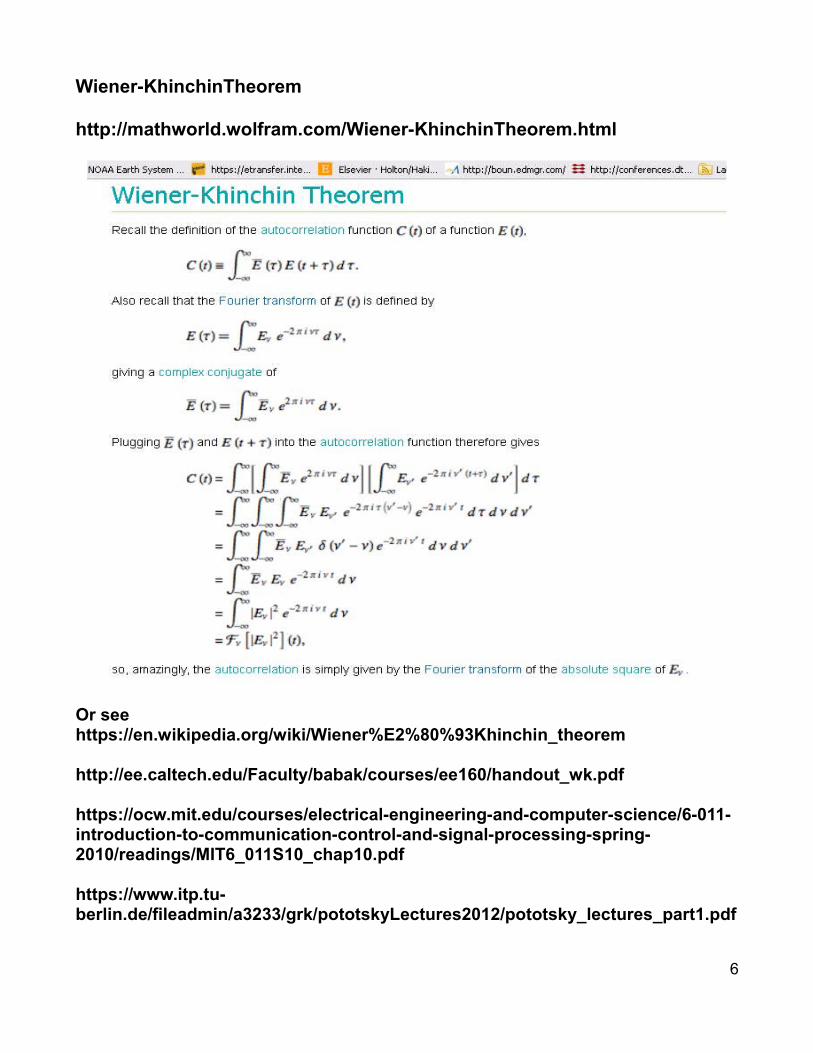
Wiener-KhinchinTheorem

http://mathworld.wolfram.com/Wiener-KhinchinTheorem.html

Or seehttps://en.wikipedia.org/wiki/Wiener%E2%80%93Khinchin_theorem

http://ee.caltech.edu/Faculty/babak/courses/ee160/handout_wk.pdf

https://ocw.mit.edu/courses/electrical-engineering-and-computer-science/6-011-introduction-to-communication-control-and-signal-processing-spring-2010/readings/MIT6_011S10_chap10.pdf

https://www.itp.tu-berlin.de/fileadmin/a3233/grk/pototskyLectures2012/pototsky_lectures_part1.pdf

6

Convolution: In mathematics, the convolution theorem states that under suitable conditions the Fourier transform of a convolution is the pointwise product of Fourier transforms. In other words, convolution in one domain (e.g., time domain) equals point-wise multiplication in the other domain (e.g., frequency domain)

The Fourier transform F(k) = or with t and ν

http://mathworld.wolfram.com/FourierTransform.html http://mathworld.wolfram.com/ConvolutionTheorem.html http://mathworld.wolfram.com/Convolution.htmlA convolution is an integral that expresses the amount of overlap of one function as it is shifted over another function. It therefore "blends" one function with another.

7

https://en.wikipedia.org/wiki/Convolution

http://www.dspguide.com/CH6.PDF in "The Scientist and Engineer's Guide toDigital Signal Processing By Steven W. Smith, Ph.D." Several chapters are relevant.

DSP = Digital Signal Processing.

8

Note these are LINEAR systems. Filtering is one example

9

From: http://www.dspguide.com/CH6.PDF in "The Scientist and Engineer's Guide toDigital Signal Processing By Steven W. Smith, Ph.D."

10

11

12

The Input Side Algorithm

13

14

Reversing x and h gives same y. Convolution is commutative. Is that true for continuous variable form? x(star)h (t) = ∫ x(t')h(t-t')dt' - integral over all t' = h(star)x

15

16

Lets try an example in R.

convolve {stats} R Documentation

Convolution of Sequences via FFTDescriptionUse the Fast Fourier Transform to compute the several kinds of convolutions of two sequences.Usageconvolve(x, y, conj = TRUE, type = c("circular", "open", "filter"))

Argumentsx, y numeric sequences of the same length to be convolved.conj logical; if TRUE, take the complex conjugate before back-transforming (default, and

used for usual convolution).type character; partially matched to "circular", "open", "filter". For "circular",

the two sequences are treated as circular, i.e., periodic.For "open" and "filter", the sequences are padded with 0s (from left and right) first; "filter" returns the middle sub-vector of "open", namely, the result of runninga weighted mean of x with weights y.

DetailsThe Fast Fourier Transform, fft, is used for efficiency.The input sequences x and y must have the same length if circular is true.Note that the usual definition of convolution of two sequences x and y is given by convolve(x, rev(y), type = "o").

Alternately use

filter {stats} R Documentation

Linear Filtering on a Time SeriesDescriptionApplies linear filtering to a univariate time series or to each series separately of a multivariate time series.Usagefilter(x, filter, method = c("convolution", "recursive"), sides = 2, circular = FALSE, init)

Argumentsx a univariate or multivariate time series.filter a vector of filter coefficients in reverse time order (as for AR or MA coefficients).method Either "convolution" or "recursive" (and can be abbreviated).

17

If "convolution" a moving average is used: if "recursive" an autoregression is used.

sides for convolution filters only. If sides = 1 the filter coefficients are for past values only; if sides = 2 they are centred around lag 0. In this case the length of the filter should be odd, but if it is even, more of the filter is forward in time than backward.

circular for convolution filters only. If TRUE, wrap the filter around the ends of the series, otherwise assume external values are missing (NA).

init for recursive filters only. Specifies the initial values of the time series just prior to the start value, in reverse time order. The default is a set of zeros.

> x=c(0,-1,-1.2,2,1.3,1.3,0.7,0,-0.8)> h=c(1.-0.5,-0.3,-0.2)

filter(x, h, method = c("convolution", "recursive"), sides = 1, circular = FALSE, init)Time Series:Start = 1 End = 9 Frequency = 1 [1] NA NA NA 2.90 0.86 0.29 -0.74 -1.00 -1.27

> y=filter(x, h, sides=1)

> plot(y, type="o", col="blue", pch=15)

18

2 4 6 8

-1.0

0.5

2.0

Index

x

1.0 1.5 2.0 2.5 3.0 3.5 4.0

-0.5

0.5

Index

h

Extra values (9,10,11) assume zeros in x. My estimated values slightly incorrect.

Suppose we us convolve?

> yy=convolve(x, rev(h), type = "o")> plot(y, type="o", col="blue", pch=15)> plot(yy, type="o", col="blue", pch=15)

19

Time

y

2 4 6 8

-10

12

3

Time

y

2 4 6 8

-10

12

3

20

Time

y

2 4 6 8

-10

12

3

2 4 6 8 10 12

-10

12

3

Index

yy

21

22

23

Compare with ARMA processes - is this MA or AR?

24