estcp cost and performance report - defense … and abbreviations (continued) vi pir...

ESTCPCost and Performance Report

ENVIRONMENTAL SECURITYTECHNOLOGY CERTIFICATION PROGRAM

U.S. Department of Defense

(EW-200938)

A Wireless Platform for Energy Efficient Building Control Retrofits

August 2012

Report Documentation Page Form ApprovedOMB No. 0704-0188

Public reporting burden for the collection of information is estimated to average 1 hour per response, including the time for reviewing instructions, searching existing data sources, gathering andmaintaining the data needed, and completing and reviewing the collection of information. Send comments regarding this burden estimate or any other aspect of this collection of information,including suggestions for reducing this burden, to Washington Headquarters Services, Directorate for Information Operations and Reports, 1215 Jefferson Davis Highway, Suite 1204, ArlingtonVA 22202-4302. Respondents should be aware that notwithstanding any other provision of law, no person shall be subject to a penalty for failing to comply with a collection of information if itdoes not display a currently valid OMB control number.

1. REPORT DATE AUG 2012

2. REPORT TYPE N/A

3. DATES COVERED -

4. TITLE AND SUBTITLE A Wireless Platform for Energy Efficient Building Control Retrofits

5a. CONTRACT NUMBER

5b. GRANT NUMBER

5c. PROGRAM ELEMENT NUMBER

6. AUTHOR(S) 5d. PROJECT NUMBER

5e. TASK NUMBER

5f. WORK UNIT NUMBER

7. PERFORMING ORGANIZATION NAME(S) AND ADDRESS(ES) ESTCP Office 4800 Mark Center Drive Suite 17D08 Alexandria, VA 22350-3605

8. PERFORMING ORGANIZATIONREPORT NUMBER

9. SPONSORING/MONITORING AGENCY NAME(S) AND ADDRESS(ES) 10. SPONSOR/MONITOR’S ACRONYM(S)

11. SPONSOR/MONITOR’S REPORT NUMBER(S)

12. DISTRIBUTION/AVAILABILITY STATEMENT Approved for public release, distribution unlimited

13. SUPPLEMENTARY NOTES The original document contains color images.

14. ABSTRACT

15. SUBJECT TERMS

16. SECURITY CLASSIFICATION OF: 17. LIMITATION OF ABSTRACT

SAR

18. NUMBEROF PAGES

50

19a. NAME OFRESPONSIBLE PERSON

a. REPORT unclassified

b. ABSTRACT unclassified

c. THIS PAGE unclassified

Standard Form 298 (Rev. 8-98) Prescribed by ANSI Std Z39-18

i

COST & PERFORMANCE REPORT Project: EW-200938

TABLE OF CONTENTS

Page

1.0 EXECUTIVE SUMMARY ................................................................................................ 1 1.1 OBJECTIVES OF THE DEMONSTRATION ....................................................... 1 1.2 TECHNOLOGY DESCTIPTION .......................................................................... 1 1.3 DEMONSTRATION RESULTS ............................................................................ 1 1.4 IMPLEMENTATION ISSUES .............................................................................. 2

2.0 INTRODUCTION .............................................................................................................. 5 2.1 BACKGROUND .................................................................................................... 5 2.2 OBJECTIVES OF THE DEMONSTRATION ....................................................... 5 2.3 REGULATORY DRIVERS ................................................................................... 6

3.0 TECHNOLOGY DESCRIPTION ...................................................................................... 7 3.1 TECHNOLOGY OVERVIEW ............................................................................... 7 3.2 ADVANTAGES AND LIMITATIONS OF THE TECHNOLOGY...................... 8

4.0 FACILITY/SITE DESCRIPTION .................................................................................... 11 4.1 FACILITY/SITE LOCATION, OPERATIONS, AND CONDITIONS .............. 11 4.2 FACILITY/SITE IMPLEMENTATION CRITERIA ........................................... 11 4.3 SITE-RELATED PERMITS AND REGULATIONS .......................................... 11

5.0 TEST DESIGN AND ISSUE RESOLUTION ................................................................. 13 5.1 CONCEPTUAL TEST DESIGN .......................................................................... 14 5.2 BASELINE CHARACTERIZATION .................................................................. 15 5.3 DESIGN AND LAYOUT OF TECHNOLOGY COMPONENTS ...................... 16

5.3.1 System Communication Architecture ....................................................... 16 5.4 HIERARCHICAL CONTROL ARCHITECTURE ............................................. 16

5.4.1 HVAC Retrofits ........................................................................................ 17 5.5 OPERATIONAL TESTING ................................................................................. 18 5.6 SAMPLING PROTOCOL .................................................................................... 18

6.0 PERFORMANCE RESULTS ........................................................................................... 21 6.1 PERFORMANCE COMPARISON BETWEEN PRE- AND

POST-RETROFIT MODES ................................................................................. 21 6.2 PERFORMANCE COMPARISON BETWEEN POST-RETROFIT AND

OPTIMIZATION MODES ................................................................................... 23

7.0 COST ASSESSMENT ...................................................................................................... 29 7.1 COST MODEL ..................................................................................................... 29 7.2 COST DRIVERS .................................................................................................. 30 7.3 COST ANALYSIS AND COMPARISON ........................................................... 31

TABLE OF CONTENTS (continued)

Page

ii

8.0 IMPLEMENTATION ISSUES ........................................................................................ 35

9.0 REFERENCES ................................................................................................................. 37 APPENDIX A POINTS OF CONTACT............................................................................... A-1

iii

LIST OF FIGURES

Page Figure 1. Schematic of the supervisory control system technology. ...................................... 8 Figure 2. System network communication architecture. ...................................................... 15 Figure 3. Hierarchical control architecture. .......................................................................... 17 Figure 4. Average zonal load conditions during the pre- and post-retrofit modes. .............. 22 Figure 5. Average set points for cold and hot deck discharge air temperatures and

supply flows. ......................................................................................................... 22 Figure 6. Illustration of HVAC energy consumption for the pre- and post-retrofit

modes. ................................................................................................................... 22 Figure 7. Average difference between set points and actual space temperature values

for pre- and post-retrofit........................................................................................ 23 Figure 8. Summary of HVAC system energy use (top) and peak power consumption

(bottom) for 2011 demonstration tests. ................................................................. 24 Figure 9. Summary of HVAC system energy use (top) and peak power consumption

(bottom) measurements from final demonstration tests in February 2012. .......... 26 Figure 10. Summary for the post retrofit and MPC modes, from demonstration tests

in February 2012, illustrating the system operation changes accomplished by the optimization algorithm. .............................................................................. 27

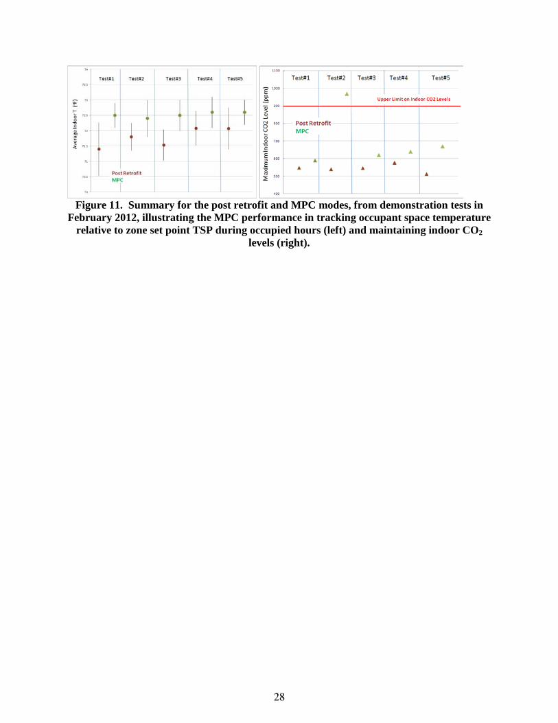
Figure 11. Summary for the post retrofit and MPC modes, from demonstration tests in February 2012, illustrating the MPC performance in tracking occupant space temperature relative to zone set point TSP during occupied hours (left) and maintaining indoor CO2 levels (right). .................................................. 28

Figure 12. Comparison of wired versus wireless as network size increases. ......................... 33 Figure 13. Cost savings using wireless as network size increases. ........................................ 34

iv

LIST OF TABLES

Page Table 1. Performance objectives. ........................................................................................ 13 Table 2. The HVAC system retrofits for all three modes of operation evaluated. ............. 15 Table 3. Retrofit items in the demonstration area. .............................................................. 16 Table 4. Cost model for wireless sensor network. .............................................................. 29 Table 5. Post-retrofit to MPC comparison for four scenarios. ............................................ 32 Table 6. Wired versus wireless comparison........................................................................ 33

v

ACRONYMS AND ABBREVIATIONS AHU Air Handling Unit ASHRAE American Society of Heating, Refrigerating and Air-Conditioning Engineers BAS building automation system BLCC Building Life-Cycle Cost BTU British thermal unit CBECS Commercial Building Energy Consumption Survey CERL Construction and Engineering Research Laboratory COTS commercial off-the-shelf CVRSME coefficient of variation of the root mean squared error DDC direct digital control DoD Department of Defense EISA Energy Independence and Security Act EO Executive Order EPACT Energy Policy Act ERDC Engineer Research and Development Center ESTCP Environmental Security Technology Certification Program HGL HydroGeoLogic, Inc. HMI human-machine interfaces HVAC heating, ventilation and air conditioning IAQ Indoor Air Quality IT information technology LCC life-cycle cost LNS LonWorks™ Network Software MPC Model Predictive Control MZU multi-zone unit NIST National Institute of Standards and Technology NMBE normalized mean bias error OA outside air OPC open connectivity ORNL Oak Ridge National Laboratory PC People Counter PI proportional-integral

ACRONYMS AND ABBREVIATIONS (continued)

vi

PIR proportional-integral-derivative RA Return Air RF radio frequency RH relative humidity RTU rooftop unit SIR savings to investment ratio TAB testing, adjusting and valance TRL technology readiness level TSP temperature set point UCB University of California, Berkeley UIUC University of Illinois at Urbana Champaign UTRC United Technologies Research Center VFD variable frequency drive WSN wireless sensor network

This page left blank intentionally.

Technical material contained in this report has been approved for public release. Mention of trade names or commercial products in this report is for informational purposes only;

no endorsement or recommendation is implied.

viii

ACKNOWLEDGEMENTS The U.S. Army Engineer Research and Development Center (ERDC) – Construction and Engineering Research Laboratory (CERL) and the University of Illinois provided a demonstration site and technical support. This includes CERL researchers David Schwenk, Joseph Bush, and Andrew Friedl along with CERL-Department of Public Works (DPW) staff Ron Huber and Clint Wilson, the CERL Information Technology (IT) staff, and University of Illinois Facilities and Services maintenance staff Bob Wright and Gary Osborne. Notably CERL researchers authored the original sequence of control, assisted with the construction scope of work. The CERL researchers, DPW staff, and University of Illinois staff provided onsite assistance with various maintenance and troubleshooting activities and advice and assistance with operation and support of the building automation system servers. Alpha Controls, the controls contractor, including Mike Boogemans, Ravi Ramrattan, Jason Vogelbaugh and others, provided an enormous amount of support installing and maintaining the building automation system for the original retrofit as well and during the technology demonstration period. Finally, the team and authors gratefully acknowledge the financial support and technical guidance provided by the Environmental Security Technology Certification Program (ESTCP) Office under the leadership of leadership Drs. Jeff Marqusee and Jim Galvin as well as the support provided by Mr. Jonathan Thigpen HydroGeoLogic, Inc. (HGL) throughout the project period of performance. The thorough review and constructive comments and suggestions provided by Mr. Glen DeWillie (HGL) for the Final Report were also highly appreciated.

1

1.0 EXECUTIVE SUMMARY

1.1 OBJECTIVES OF THE DEMONSTRATION

The primary objectives of this project are to demonstrate: (1) energy efficiency gains achievable in small- to medium-sized buildings with MPC-based whole-building optimal control and (2) reduction in first costs achievable with a wireless sensor network (WSN)-based building heating, ventilation and air conditioning (HVAC) control system compared to a conventional wired system. The second objective is key because first cost is a barrier to wider application of advanced HVAC control and 70% of the first cost is attributed to installation (wiring) and commissioning.

1.2 TECHNOLOGY DESCTIPTION

This project demonstrated an advanced energy management and control system in an existing building in U.S. Army’s Construction and Engineering Research Laboratory (CERL) in Urbana-Champaign, IL. The medium-size office building underwent a retrofit of the HVAC system and controls employing a technology called optimal Model Predictive Control (MPC) which offers significant potential for saving energy by providing a means to dynamically optimize various sub-systems, such as fans, cooling and heating coils, to take advantage of building utilization and weather patterns, and utility rate structures. The United Technologies Research Center (UTRC)-led team, partnered with Army-CERL facility staff and researchers at the Oak Ridge National Laboratory (ORNL) and the University of California Berkeley, tested as a proof-of-concept the on-line implementation of model-based predictive and optimal control of the HVAC system in a 7000 sq. ft. portion of the CERL building. The system was retrofitted with a commercial off-the-shelf open protocol building automation system. The existing controls operated the HVAC system continuously during the day, maintained fixed temperature set points in the Air Handling Unit (AHU) heating and cooling deck discharges and used a fixed outdoor air fraction for ventilation in the building. The MPC approach aimed to increase system efficiency by continuous adjustment of the system schedule of operation, heating and cooling set points, and fresh air levels brought into the building, based on predicted and measured occupancy levels, internal loads, and weather forecasts. System and indoor environment measurements of supply air temperatures and airflows, occupancy, zonal temperature, relative humidity, and CO2 levels were used to learn relevant HVAC equipment, thermal and occupancy models on-line and to configure control design. Sub-metering was used to establish baseline energy consumption and to verify performance improvements. To reduce installation cost, wireless sensors were utilized wherever possible, particularly for occupancy sensing and thermal comfort. The WSN self-configures routing of data through a gateway to a central control computer that hosts the algorithms.

1.3 DEMONSTRATION RESULTS

A multi-variable optimization problem to minimize energy consumption and cost while guaranteeing zonal comfort over a 3 hour predictive horizon was formulated and solved periodically on line. The algorithms were integrated with the building automation system and evaluated experimentally from July 2011 to February 2012. A 55-65% reduction in HVAC

2

system energy use was demonstrated while improving occupant comfort. Of this, nearly 35% improvement was achieved via off-line adjustments of the system’s operation schedule and heuristic adjustments of the heating and cooling coil set points. This post retrofit state of the HVAC system involved implementation of direct digital controls (DDC) and a basic building automation system. The additional improvement of 60-80% relative to the post-retrofit heuristic implementation, was accomplished by on line dynamic optimization of the building. A 10-15% installation cost reduction was accomplished by use of a robust WSN versus a fully wired network. The advanced control system and algorithms were monitored by UTRC and CERL until April 2012. Following this testing and evaluation, the CERL facility management team reverted back to the post retrofit mode in anticipation of further upgrades to the remainder of the facility. It should be noted that the present implementation of optimal controls was for a specific form of central building HVAC system involving a dual deck configuration. Such systems are prevalent in older buildings, of which there are many in the Department of Defense (DoD) stock, and are more prone to energy waste from system duct losses and leakages, compared to single deck HVAC systems (deployed more commonly now). This could explain some of the large energy savings accomplished when going from a pneumatic control approach for 24/7 operation to a DDC mode operation (considered as a post-retrofit baseline for optimal control mode). Furthermore, a more fine tuned DDC mode control strategy involving reset of the cooling and heating deck set points based on outside weather, rather than a seasonal setting (as employed at the demonstration site), would have captured some of the savings achieved by the optimal scheme. Finally, much of the optimal control mode performance data was obtained for heating season operation, although some cooling mode data was captured between July and September 2012, primarily for pneumatic and DDC modes of operation. More detailed assessments and analysis for different variants of the central HVAC system and of baseline DDC mode control approaches are needed to ascertain the variability in the energy use and peak power reduction benefits across DoD stock. The model-based control methodology pursued here can be extended to hydronic heating and cooling systems where variable speed technologies are becoming prevalent and robust, but multivariable optimal control methodologies are lacking. The building HVAC control technology is applicable to small- and medium-sized buildings, which represent a significant portion of the DoD building stock. The demonstrated energy savings of more than 60% reduction in HVAC system energy use is estimated to lead to nearly 20% building level energy use reduction (assuming conservatively that HVAC systems constitute 30% of total building energy use). This represents significant progress toward the 30% gains in energy efficiency beyond 2003 levels mandated by Executive Order 13423. Renovations and retrofits are driven toward a 20% savings goal relative to pre-retrofit 2003 levels, and by this measure the improvements demonstrated in the present program represent the potential to meet the goal through broader scale implementation of optimal control technology alone.

1.4 IMPLEMENTATION ISSUES

Key challenges were identified in the additional cost to install the WSNs, particularly the skill level and familiarity required by the contractor to deploy them. This adversely impacted the installed cost gains that were accomplished through the use of a wireless sensor infrastructure. Furthermore, the lack of familiarity with, and related perceived risk in, the maintenance for the

3

optimal control platform, which utilizes Matlab and optimization toolboxes, was an impediment to longer-term sustained deployment of the promising technology at the demonstration site. Finally, technical challenges remain in the scalability and level of automation required to obtain relevant dynamic system models, and for the configuration and commissioning of the optimal control algorithms with the building management system.

5

2.0 INTRODUCTION

2.1 BACKGROUND

For the foreseeable future, the largest opportunity to reduce DoD energy consumption will come from retrofits and renovations to its existing 343,867 buildings. DoD facilities in fiscal year (FY) 2007 consumed 104,416 British thermal units (Btu)/sq. ft., an improvement over the baseline (136,744 BTU/Sq. ft. in FY 1985 for standard buildings and 213,349 Btu/sq. ft. for industrial and lab facilities) but it still lags the national average (see Commercial Building Energy Consumption Survey [CBECS] [2]) of 91,000 Btu/sq. ft. (for 2003). A promising technology for realizing energy efficiency is whole-building optimal control, which has the potential to reduce building energy consumption by 3-10% (0.5-1.7 of the 17 quads of energy consumed by U.S. commercial buildings) [3]. This technology does so by continuously adjusting HVAC ventilation rates and temperature set-points to match building occupancy and weather loads. While such loads dominate the energy usage in office/administrative, lodging/barracks, warehouse, retail and many other buildings, other specialized buildings such as hospitals, data centers and dining facilities are dominated by other process loads, which are typically not controllable since they are essential for the mission critical services they provide. In contrast, the majority of existing buildings are designed and operated based on a maximum occupancy and a worst-case “design day” leading to excessive ventilation and air conditioning. A barrier to broad deployment of this technology to the existing building stock is the high first cost of building HVAC control systems. On average, installation (largely wiring and sensor addressing) and commissioning of building control systems account for 70% of the installed costs and the result is a one to ten year simple payback for optimized building controls [3]. What is needed is a scalable, robust building control platform consisting of sensing, computation, and actuation that is suitable for retrofit applications—especially facilities not served by a building management system—at an installed cost significantly below what is common today. In this project, UTRC, in partnership with ORNL, and the University of California, Berkeley (UCB) developed a control platform and demonstrated both the first cost and operational cost benefits of whole-building optimal HVAC control. The system consists of (1) a WSN interfaced via an industry-standard communications protocol to a commercially available, networked HVAC control system, and (2) an optimal control algorithm that reduces wasteful energy consumption and interfaces to existing building HVAC equipment.

2.2 OBJECTIVES OF THE DEMONSTRATION

The specific technical objectives of the demonstration were (1) to develop and deploy a WSN-based HVAC control system to a technology maturity level that would enable commercialization leading to wide-scale deployment; (2) to demonstrate that the control system can reduce peak electrical demand by 10% and monthly summer energy consumption by 15% while meeting required indoor environment comfort requirements; and (3) to demonstrate a 50% reduction in the costs of system installation, relative to that for a fully wired retrofit solution. The system was operated over a twelve month period to both mature the technology and measure its performance across a wide range of operating conditions.

6

2.3 REGULATORY DRIVERS

The Energy Policy Act (EPACT) of 1992, Energy Independence and Security Act (EISA) of 2007 (Title IV, Subtitle C) and Executive Order (EO) 13423 mandate DoD to measure and improve facility energy efficiency by 30% beyond 2003 levels. EO 13514 requires reducing energy intensity in agency buildings. EO 13423 is more specific and requires DoD to “improve energy efficiency and reduce greenhouse gas emissions, through reduction of energy intensity by (i) 3% annually through the end of FY 2015, or (ii) 30% by the end of FY 2015, relative to FY 2003, and ensure that (i) new construction and major renovation comply with the Guiding Principles, and (ii) 15% of the existing Federal capital asset building inventory of the agency as of the end of FY 2015 incorporates the sustainable practices in the Guiding Principles.

7

3.0 TECHNOLOGY DESCRIPTION

3.1 TECHNOLOGY OVERVIEW

The technology consists of two main elements: (1) a WSN interfaced via an industry-standard communications protocol to a commercially available, networked HVAC control system, and (2) an optimal control algorithm that reduces wasteful energy consumption and interfaces to existing building HVAC equipment. These two elements are detailed in the following sub-sections. The use of WSNs provides three distinct advantages when compared to a wired system. First, it reduces installation costs relative to a baseline wired system by eliminating the need to run signal and power wires to each sensor and also by its ability for self configuration. Second, the flexible and optimal sensor placement enables more effective control. Sensor placement could be adjusted during operation as a troubleshooting measure, and sensors can be added or removed as the building usage evolves. Third, the elimination of wires offers a critical advantage and cost reduction means for retro-commissioning in old buildings or those where access is expensive (due to issues such as asbestos removal or management). A detailed cost comparison between wired and wireless implementation of the sensor network is performed in Section 7.0 to assist future implementations. A reliable and secure WSN was used to provide a majority of the monitoring capabilities for the project. The technology readiness level (TRL) of the WSN technology was TRL 5 at the beginning of the project and extended to TRL 6-7 towards the end. WSN is used to measure temperature, relative humidity, CO2, passive infrared, flow, and pressure. The WSN is self configured by routing packets automatically across the network and adjusting network parameters (routing information) as the conditions within the building change, providing a degree of robustness. Interoperability is the key enabler to retro-commissioning in existing buildings. A gateway is used to make WSN transparent to the existing building automation system. The installer would only have to map the physical address of each node to the logical address of each node. Wireless sensors also provide specific maintenance and security management requirements. Low-power, low-duty cycle radio technology used in the project has a projected lifetime of three years. IEEE 802.15.4-based wireless modules are used for the deployment. AES-128-bit encryption is part of the standard. A determination of whether this met all the relevant DoD security requirements has not formally been made. The demonstration system, while not formally qualified, is roughly at FIPS 140-2 Level 1, but can be extended to include higher-level requirements. This would require incorporation of the cryptographic and physical protection mechanisms as defined by the relevant standards. The WSN system is architected in a way to provide fallback to non-optimal operation in-case any failures arise in the network. A model-based predictive supervisory controller, illustrated in Figure 1, adjusts outside air ventilation rates and zonal temperature set points within comfort and Indoor Air Quality (IAQ) constraints (prescribed by American Society of Heating, Refrigerating and Air-Conditioning Engineers [ASHRAE] 62.1) to minimize a weighted combination of energy consumption and

8

peak energy demand over a 4-8 hour horizon. The algorithm is executed continuously, and monitors weather, indoor environmental conditions, and occupancy levels, to ensure that the building operates within comfort and IAQ constraints, while minimizing the energy cost function. The control is at a supervisory level; meaning it determines reference values for local feedback loops, but does not affect the zonal temperature feedback loops themselves, which remain in place to regulate temperature. The cost function can be adjusted to emphasize peak power demand or energy consumption over time and can also be adjusted to modify comfort or IAQ constraints, providing a degree of flexibility to building operation. The resulting supervisory control law effectively exploits passive energy storage in both envelope and air.

Figure 1. Schematic of the supervisory control system technology.

In contrast, conventional HVAC controls are only reactive, using feedback to drive set points to fixed values (although there may be set-backs based on a schedule) and do not exploit energy storage optimally. The technology is applicable to a wide variety of buildings that are served by systems ranging from built-up systems to rooftop units (RTU), provided the outside air ratio, system temperature and flow set points, and zonal temperature set points are available and adjustable parameters. The methodology of load estimation and predictive model-based performance optimization is also applicable to the control of district systems, such as those for cooling and heating, although many of the sub-systems and thermal load models would be quite different from those encountered in building-level HVAC systems.

3.2 ADVANTAGES AND LIMITATIONS OF THE TECHNOLOGY

The advantages of the WSN over a wired installation include optimal sensor placement, significantly reduced installation costs (especially retrofit), increased sensing locations, and reduced cost of additional sensing (scalability). The limitations of WSN include time-varying

9

nature of the radio frequency (RF) channel requiring site-specific optimization, optimal configuration management over time, training of the facility operational personnel, and maintenance of WSN. This project addresses the limitations and provides guidance and tools to reduce the uncertainties involved. The steps taken to ensure robust network operation are summarized below:

1. Understand the ambient RF environment. Although we performed thorough RF measurements, minimal understanding of the existing networks and frequencies of operation is required to exploit the frequency and spatial diversity.

2. Incorporate temporal channel mobility. Each node in the network constantly monitors the 16 channels in the 2.4 Giga Hertz band and identifies the 4 channels with least interference. The network hops across these channels to maximize performance.

3. Address spatial density by mains powered wireless repeaters which extend the network range and reduce the transmit power on each node improving network lifetime.

4. The key limitation of a successful WSN deployment is interoperability with building automation systems. We addressed this by using a gateway capable of translating 802.15.4 packets in to LonWorks addressable “points.”

5. Ensure that network installed is compliant with site IT requirements. Broader compliance issues related to information assurance requirements for DoD sites were not explored.

Robust and accurate occupancy estimation algorithms are useful for estimating internal loads in buildings. Motion detectors are not typically integrated into the HVAC system controls and do not measure the number of occupants. While temperature and CO2 sensors provide better but indirect measures of actual occupancy, their response is slow and can be grossly inaccurate without frequent calibration. A multi-sensor data and model driven procedure was demonstrated to generate and predict accurate occupancy estimates. Simple representations of occupant traffic patterns were learned and combined with real-time estimates of occupancy distributions in buildings. An occupancy estimation error of <10% was demonstrated using cameras, CO2 sensor, and PIR sensors combined with learned historical facility usage information. This is a substantial improvement over the error using CO2 or video sensors alone. MPC strategies were used successfully in applications with large time delays, larger numbers of set-points, and constraints. As opposed to currently implemented rule-based control policies with fixed set-points, schedules, and sequences, predictive strategies use weather forecasts and occupancy patterns to predict loads over a four to eight hour time horizon and use the passive energy stored in the building envelope and air. To accurately predict the loads, algorithms rely on physics-based models for water-to-air thermal energy transfers and efficiency maps for HVAC equipment. A limitation of this approach is dependency on the accuracy of these models. The numerous sensor measurements will help mitigate this risk by calibrating the models’ parameters. Another limitation is the number of optimization variables; a large number of variables and constraints can result in a long search time before the optimization algorithm

10

converges on the optimal solution. Selecting appropriate values for the optimization horizon length and update frequency of the actuator inputs will mitigate this risk.

11

4.0 FACILITY/SITE DESCRIPTION

4.1 FACILITY/SITE LOCATION, OPERATIONS, AND CONDITIONS

The demonstration targeted small and medium sized buildings and was conducted at the U.S. Army’s Construction Engineering Research Laboratory (CERL) [4], located in Champaign, IL. The CERL site was ideal for this demonstration. It includes medium sized mixed-use buildings approximately 20-40 years in age served by both a central plant and also a diverse range of RTUs and split air conditioning systems. Its age, mixed use (office and laboratory), and HVAC system diversity makes it well suited to a controls retrofit. Moreover, Champaign IL offers weather diversity enabling testing under a broad range of conditions, and the CERL site can help facilitate transition since the demonstration is aligned with its mission. The demonstration area is served by a constant volume multi-zone system, serving five zones. The HVAC equipment in the demonstration area is controlled using pneumatic actuators that maintain the occupant-selected thermostat temperatures by controlling the position of dampers (outside air, supply, return, and zone air-flow), and temperature set-points in hot deck and cold deck coils. Facility wide, CERL is upgrading the control equipment to digital controllers and integrating it in a LonWorks communication network that enables both automatic monitoring (near-term) and control (long-term) of the HVAC components. Wonderware software is being installed as part of the upgrading activities currently in progress at CERL (in parallel to this project activity). The existing control schedule is fixed, and independent of weather forecast and occupancy. Due to the lack of adequate instrumentation, integrated controllers and monitoring systems, it is unclear to what extent the IAQ constraints were being met in the pre-retrofit condition, or what the current energy consumption of the system was.

4.2 FACILITY/SITE IMPLEMENTATION CRITERIA

The technology developed in this project is applicable to existing buildings with sub-optimal controls, and not served by a building automation system. Buildings that are not served by digital controls provide the best opportunity for deploying the technology developed. While climate zones with four distinct seasons will benefit from the technology other climate zones are also applicable. Buildings with existing building automation need careful interoperability considerations for deploying this technology. This technology can be applied to typical commercial buildings served by packaged RTUs or built-up systems.

4.3 SITE-RELATED PERMITS AND REGULATIONS

The facility selected for demonstration is owned by the University of Illinois at Urbana Champaign (UIUC) and leased by CERL. The retrofits required were reviewed to ensure consistency with CERL and DoD standards for procurement through sub-contractors, installation and commissioning, using an existing controls sub-contractor, Alpha Controls, previously approved for CERL site work. UIUC building standards were followed to the extent possible while being consistent with project schedule and budget constraints. Deviations from UIUC standards were reviewed with CERL. The subcontractor performing the retrofits was responsible for obtaining local permits and ensuring compliance with building HVAC codes. Necessary approvals for installing and programming the building automation system (BAS) and required IT

12

approvals were obtained in close coordination with CERL facility and IT. The remote VPN connection required for the demonstration experiments was approved by CERL facility and IT and a separate computer from CERL was provided to UTRC team to conduct experiments remotely from UTRC location in East Hartford, CT. ORNL obtained the required approvals from CERL for installing RF devices on-site. The frequency band and protocols used for wireless communication were reviewed with the designated IT and security officials at CERL as part of the approval process. There were no major obstacles encountered in the BAS and WSN installation due to early and close engagement with CERL research, facility management and IT staff. Typical lead times for the required approvals that concerned IT were on the order of one month, but could be longer depending on other on site commitments.

13

5.0 TEST DESIGN AND ISSUE RESOLUTION

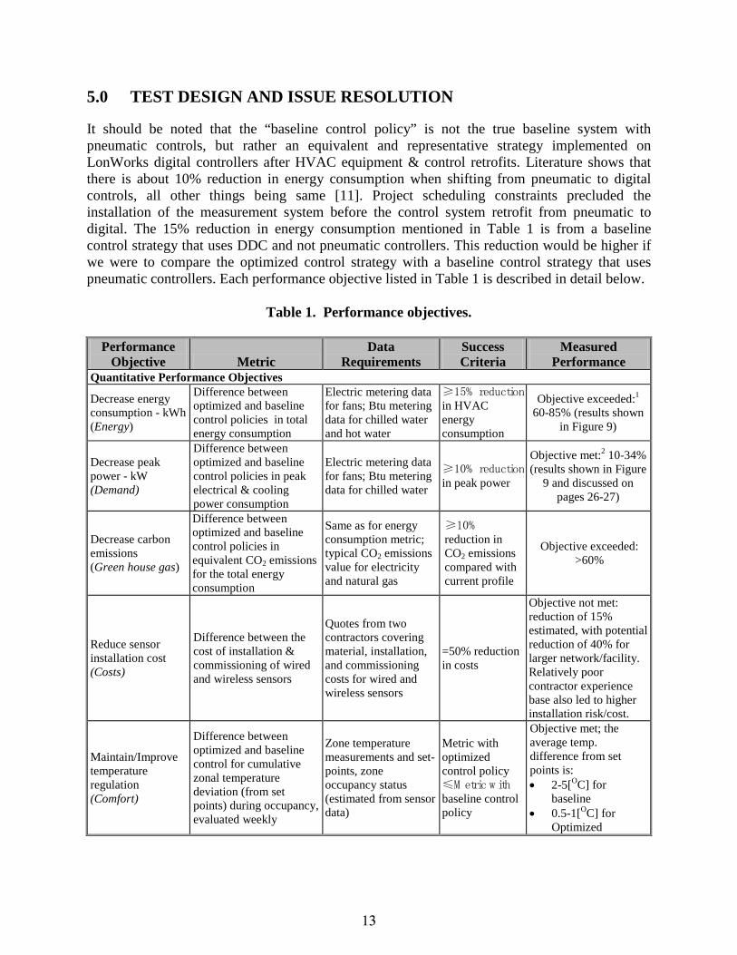
It should be noted that the “baseline control policy” is not the true baseline system with pneumatic controls, but rather an equivalent and representative strategy implemented on LonWorks digital controllers after HVAC equipment & control retrofits. Literature shows that there is about 10% reduction in energy consumption when shifting from pneumatic to digital controls, all other things being same [11]. Project scheduling constraints precluded the installation of the measurement system before the control system retrofit from pneumatic to digital. The 15% reduction in energy consumption mentioned in Table 1 is from a baseline control strategy that uses DDC and not pneumatic controllers. This reduction would be higher if we were to compare the optimized control strategy with a baseline control strategy that uses pneumatic controllers. Each performance objective listed in Table 1 is described in detail below.

Table 1. Performance objectives.

Performance

Objective Metric Data

Requirements Success Criteria

Measured Performance

Quantitative Performance Objectives

Decrease energy consumption - kWh (Energy)

Difference between optimized and baseline control policies in total energy consumption

Electric metering data for fans; Btu metering data for chilled water and hot water

≥15% reduction in HVAC energy consumption

Objective exceeded:1 60-85% (results shown

in Figure 9)

Decrease peak power - kW (Demand)

Difference between optimized and baseline control policies in peak electrical & cooling power consumption

Electric metering data for fans; Btu metering data for chilled water

≥10% reduction in peak power

Objective met:2 10-34% (results shown in Figure

9 and discussed on pages 26-27)

Decrease carbon emissions (Green house gas)

Difference between optimized and baseline control policies in equivalent CO2 emissions for the total energy consumption

Same as for energy consumption metric; typical CO2 emissions value for electricity and natural gas

≥10% reduction in CO2 emissions compared with current profile

Objective exceeded: >60%

Reduce sensor installation cost (Costs)

Difference between the cost of installation & commissioning of wired and wireless sensors

Quotes from two contractors covering material, installation, and commissioning costs for wired and wireless sensors

=50% reduction in costs

Objective not met: reduction of 15% estimated, with potential reduction of 40% for larger network/facility. Relatively poor contractor experience base also led to higher installation risk/cost.

Maintain/Improve temperature regulation (Comfort)

Difference between optimized and baseline control for cumulative zonal temperature deviation (from set points) during occupancy, evaluated weekly

Zone temperature measurements and set-points, zone occupancy status (estimated from sensor data)

Metric with optimized control policy ≤M etric w ith baseline control policy

Objective met; the average temp. difference from set points is: • 2-5[OC] for

baseline • 0.5-1[OC] for

Optimized

14

Table 1. Performance objectives (continued).

Performance Objective Metric

Data Requirements

Success Criteria

Measured Performance

Minimize occupancy estimation error (Models)

Mean percentage error between actual and estimated occupancy levels

Occupancy sensor data and ground truth/simulated occupancy data

≤20% estimation error

Objective met: ≤15%

Qualitative Performance Objectives

Maintainability Maintenance effort for proposed system (WSN and MPC)

Records of component maintenance/replacement and system downtime (frequency and duration) for proposed and baseline systems;

Expected maintenance effort similar to existing wired sensors and baseline control system

The WSN for final MPC implementation is a subset of the original network deployed, and associated maintenance costs are nominal (also see savings to investment ratio [SIR] estimate).

Ease of use

Ability of CERL facilities staff to operate/tune the proposed controller and maintain WSN after reasonable training

Feedback from CERL facility staff/management on ease of operation and maintenance

Trained facility staff is able to maintain the WSN and operate/tune the new controller. Minimal call backs to team following project completion.

CERL staff is familiar with post retrofit control system and provided documentation. There have been no call backs. MPC system was removed. Lack of familiarity with Matlab and associated software maintenance hindered MPC adoption.

1 Performance data gathered extensively for transition and heating season when operating the optimal control technology mode. Cooling season data only available for pneumatic (pre-) to DDC (post-) retrofit conversion. 2 Only heating thermal power was considered for this objective due to availability of only Winter season experimental data for the refined optimization algorithm.

5.1 CONCEPTUAL TEST DESIGN

The overall experiment consisted of three control modes that were implemented for various periods of time (days to weeks); also see Table 2. These operational modes are:

1. Baseline, or pre-retrofit, control strategy – this strategy mimics the control strategy that the demonstration system used when it was actuated by a pneumatic system.

2. Normal, or post-retrofit, control strategy – updated control strategy that takes advantage of the DDC controls and retrofits, and uses heuristic rules for controlling set points.

3. Advanced, or optimal, control strategy – the advanced MPC strategy that was demonstrated in this project.

15

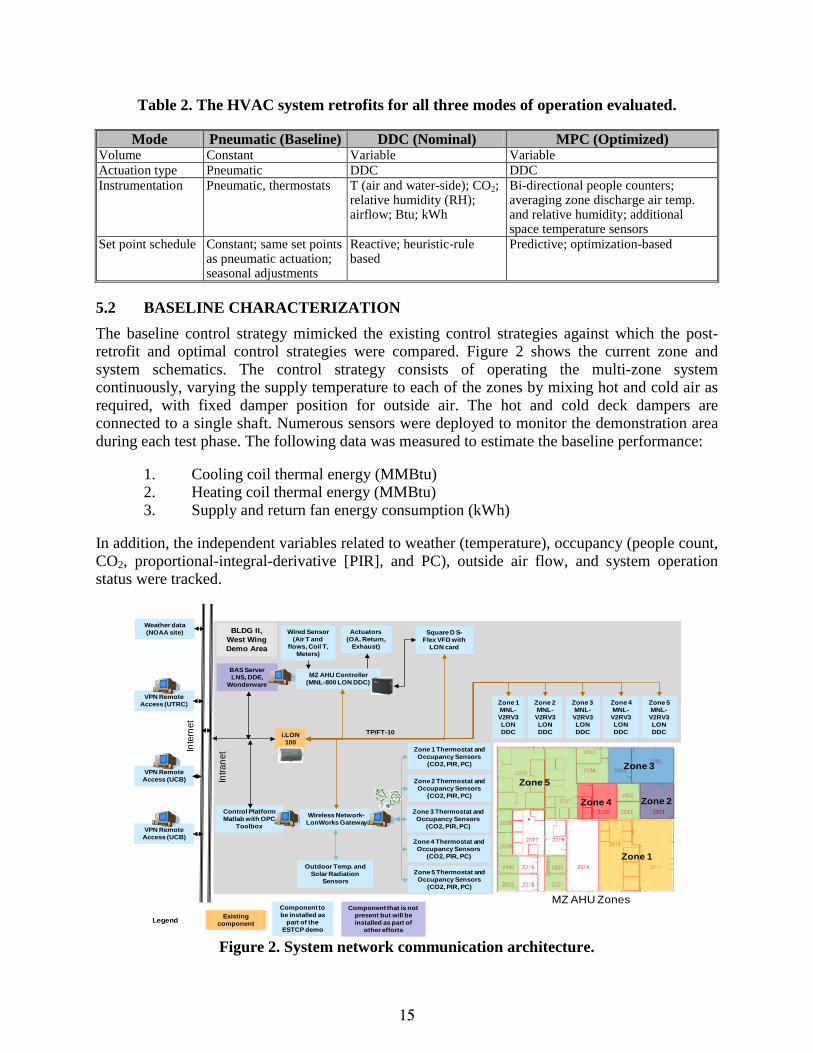
Table 2. The HVAC system retrofits for all three modes of operation evaluated.

Mode Pneumatic (Baseline) DDC (Nominal) MPC (Optimized) Volume Constant Variable Variable Actuation type Pneumatic DDC DDC Instrumentation Pneumatic, thermostats T (air and water-side); CO2;

relative humidity (RH); airflow; Btu; kWh

Bi-directional people counters; averaging zone discharge air temp. and relative humidity; additional space temperature sensors

Set point schedule Constant; same set points as pneumatic actuation; seasonal adjustments

Reactive; heuristic-rule based

Predictive; optimization-based

5.2 BASELINE CHARACTERIZATION

The baseline control strategy mimicked the existing control strategies against which the post-retrofit and optimal control strategies were compared. Figure 2 shows the current zone and system schematics. The control strategy consists of operating the multi-zone system continuously, varying the supply temperature to each of the zones by mixing hot and cold air as required, with fixed damper position for outside air. The hot and cold deck dampers are connected to a single shaft. Numerous sensors were deployed to monitor the demonstration area during each test phase. The following data was measured to estimate the baseline performance:

1. Cooling coil thermal energy (MMBtu) 2. Heating coil thermal energy (MMBtu) 3. Supply and return fan energy consumption (kWh)

In addition, the independent variables related to weather (temperature), occupancy (people count, CO2, proportional-integral-derivative [PIR], and PC), outside air flow, and system operation status were tracked.

Figure 2. System network communication architecture.

TP/FT-10

BLDG II, West Wing Demo Area

i.LON 100

Wired Sensor (Air T and

flows, Coil T, Meters)

Zone 1 Thermostat and Occupancy Sensors

(CO2, PIR, PC)

LegendExisting

component

Component to be installed as

part of the ESTCP demo

Component that is not present but will be installed as part of

other efforts

BAS ServerLNS, DDE,

Wonderware

Control PlatformMatlab with OPC

Toolbox

Intra

net

VPN Remote Access (UTRC)

VPN Remote Access (UCB)

VPN Remote Access (UCB)

Weather data (NOAA site)

MZ AHU Controller (MNL-800 LON DDC)

Actuators(OA, Return,

Exhaust)

Zone 5MNL-V2RV3 LON DDC

Square D S-Flex VFD with

LON card

Wireless Network-LonWorks Gateway


(CO2, PIR, PC)


(CO2, PIR, PC)


(CO2, PIR, PC)


(CO2, PIR, PC)

MZ AHU Zones

Outdoor Temp. and Solar Radiation

Sensors





Zone 1

Zone 2

Zone 3

Zone 4

Zone 5

Inte

rnet

16

The retrofit tasks for the baseline retrofit are described in Table 3. The retrofit was implemented between May and August 2010.

Table 3. Retrofit items in the demonstration area.

Task No. Description 1. Multi-zone unit (MZU) controllers retrofit, from pneumatic to DDC, and integration to existing

LonWorks network 2. Zone airflow controllers retrofit and integration 3. Variable frequency drive installation and integration for supply fan and return fan 4. Control sequences implementation in Building Management System software 5. Zone 1 and Zone 3 re-ducting and electrical valves installation 6. Sequence of operation generation for baseline and post-retrofit controllers 7. Testing, adjusting & balance (TAB)

5.3 DESIGN AND LAYOUT OF TECHNOLOGY COMPONENTS

5.3.1 System Communication Architecture

The overall architecture of the controls platform and its integration with the existing LonWorks network was shown in Figure 2. The implemented architecture was built on and integrated with CERL’s LonWorks-based system consisting of:

• A network controller, i.LON 100, and TP/FT-10 cabling. All the local controllers for the MZU unit and zones communicate via this network. They receive updated set point values and system status commands and send updated sensor values.

• Wonderware BAS and LonWorks™ Network Servers (LNS) that are installed under separate projects at CERL. Communication between the Wonderware and LNS is based on the open connectivity (OPC) protocol to ensure compatibility with the communication protocol with the optimization platform.

• OPC server installed on the BAS server, enabling primarily communication between the two levels of the supervisory control architecture, the BAS server, and the optimization computer. All the sensor, actuator, and set points are mapped accordingly between the server and client to ensure consistent communication.

• Wireless platform consisting of a gateway between the WSN and LNS servers. The gateway enables communication of real-time sensor measurements to the LNS and optimization platform.

• Laptops at UTRC, UCB, and ORNL sites were connected remotely to the optimization and wireless platforms for uploading and analyzing data, and to update the algorithms.

5.4 HIERARCHICAL CONTROL ARCHITECTURE

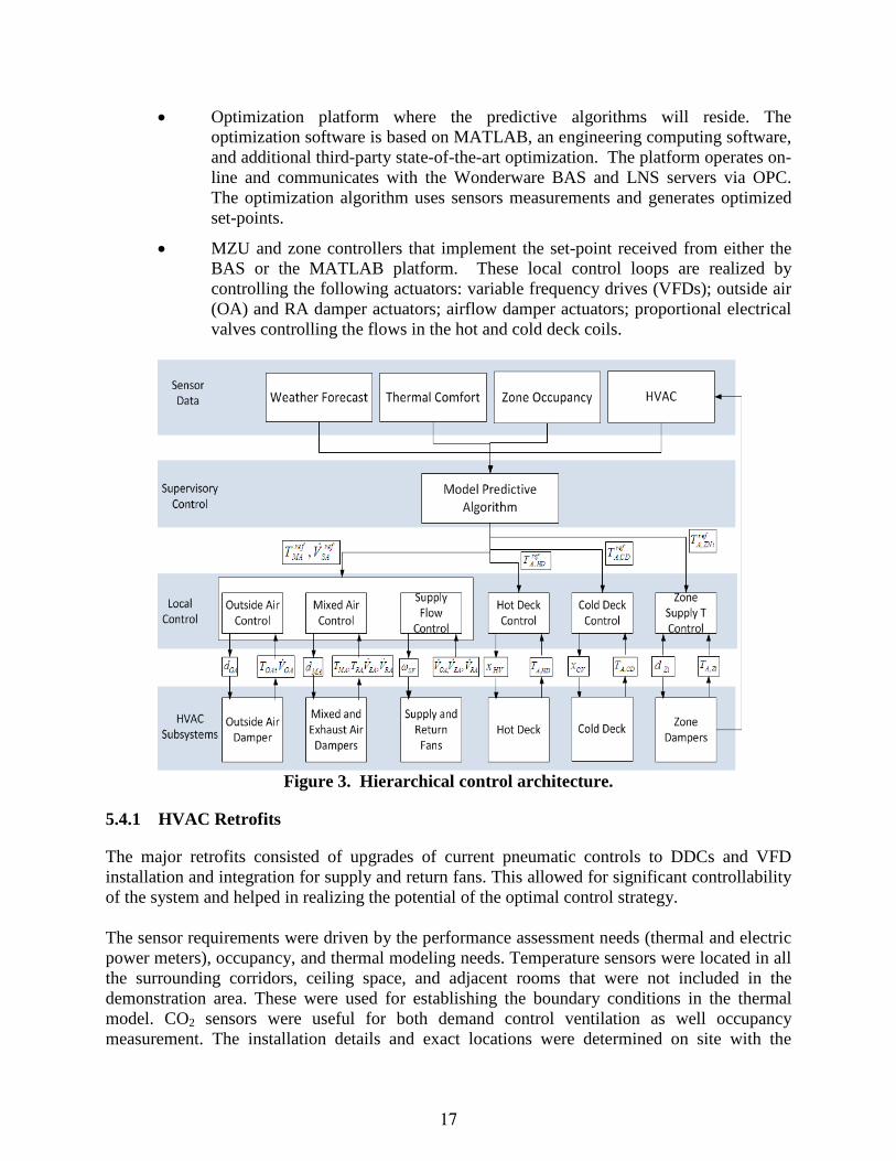
The system architecture was designed to enable implementation of the supervisory control architecture with two main layers, as illustrated in Figure 3:

17

• Optimization platform where the predictive algorithms will reside. The optimization software is based on MATLAB, an engineering computing software, and additional third-party state-of-the-art optimization. The platform operates on-line and communicates with the Wonderware BAS and LNS servers via OPC. The optimization algorithm uses sensors measurements and generates optimized set-points.

• MZU and zone controllers that implement the set-point received from either the BAS or the MATLAB platform. These local control loops are realized by controlling the following actuators: variable frequency drives (VFDs); outside air (OA) and RA damper actuators; airflow damper actuators; proportional electrical valves controlling the flows in the hot and cold deck coils.

Figure 3. Hierarchical control architecture.

5.4.1 HVAC Retrofits

The major retrofits consisted of upgrades of current pneumatic controls to DDCs and VFD installation and integration for supply and return fans. This allowed for significant controllability of the system and helped in realizing the potential of the optimal control strategy. The sensor requirements were driven by the performance assessment needs (thermal and electric power meters), occupancy, and thermal modeling needs. Temperature sensors were located in all the surrounding corridors, ceiling space, and adjacent rooms that were not included in the demonstration area. These were used for establishing the boundary conditions in the thermal model. CO2 sensors were useful for both demand control ventilation as well occupancy measurement. The installation details and exact locations were determined on site with the

18

subcontractor who installed and calibrated the equipment. The installation of low and medium priority sensors were determined by budget constraints. See the Final Report for illustrations of the HVAC system and demonstration site.

5.5 OPERATIONAL TESTING

For the retrofits, the contractor commissioned the system to operate in the post-retrofit mode, installed the required software to enable communication with the WSN and with the optimization computer, and programmed the set point overrides for various modes. The team conducted tests to check the integration of all the system components and communication between them. Tests were conducted to understand the performance of occupancy related sensors and the WSN. Before beginning the data collection for the three control modes, the MPC was tuned. This involved collecting data for two weeks for calibrating the building model thermal states and energy consumption estimation. Occupancy sensor tests at UTRC and CERL – For the demonstration site, infrared motion sensors, CO2 sensors, and people counter sensors were deployed in occupied spaces, public passageways, and entrances and exits respectively. The wireless sensors for occupancy measurements were deployed in a small office building environment at UTRC first to characterize the sensor performance in the built environment. This involved measurements of the occupancy levels under a variety of test conditions (e.g., with heavy occupant traffic and sparse occupancy) to establish statistical bounds on the sensor accuracy and performance over extended periods of time. Similar experiments and characterization were conducted at CERL involving larger scale deployment of the above-mentioned occupancy sensors at specified locations. Pre-retrofit control strategy test period – The simplified control strategy mimicked the current pneumatic controls. The system was run as though it would operate twenty-four hours, seven days a week. The VFDs were set at 100%, the hot and cold deck temperatures at constant value of 120°F and 55°F respectively, and OA damper position was set at the current level. Post-retrofit control strategy test period – The post-retrofit control strategy consisted of operating the fan at variable speeds, resetting the cold and hot deck temperatures based on zonal calls for heating/cooling, OA control based on critical zone CO2, and time based on/off schedule for operating the system based on typical occupancy patterns. Optimal control strategy test period – Based on the predicted external and internal loads, the MPC algorithm generated optimal set-points for OA, supply hot deck and cold deck temperature, flows to each space, and fan speed. In this mode, the generated set-points overrode the local controller set-points.

5.6 SAMPLING PROTOCOL

The three control modes were run sequentially whenever possible to get performance data for different seasons and indoor usage. Each option spanned multiple days with warm-up scenarios, before switching to the next option. The data were collected at fifteen minute intervals, and spanned both energy consumption related data as well as zonal conditions (temperature, CO2, and occupancy).

19

Calibration of Reference Model for MPC: The thermal network model represents the performance of the building envelope, HVAC, and control systems. Metering data for fan electricity, chilled water usage, and hot water usage were used to calibrate and validate the model. Some monitored data such as real-time weather data were processed to provide inputs for the model. The internal loads including plug load and lighting load were assumed based on inputs from CERL team with respect to typical lighting wattages and internal equipment in each space, and applied as inputs to the reference model; limited measurements of plug loads were also carried out by deploying CT meters in the facility over an extended period of few weeks. The calibration aimed for ±10% normalized mean bias error (NMBE) and ±30% for coefficient of variation of the root mean square error (CVRSME) as per ASHRAE guideline 14-2002 [12].

21

6.0 PERFORMANCE RESULTS

The performance of the retrofitted system, as summarized in Table 1, was determined from recorded measurement data. A significant challenge in estimating the energy savings, as is the case for industrial applications, is the inconsistency in the weather and usage patterns. The energy savings, the approach, and the pair-wise comparison between the three modes of operation are discussed in the following two sub-sections.

6.1 PERFORMANCE COMPARISON BETWEEN PRE- AND POST-RETROFIT MODES

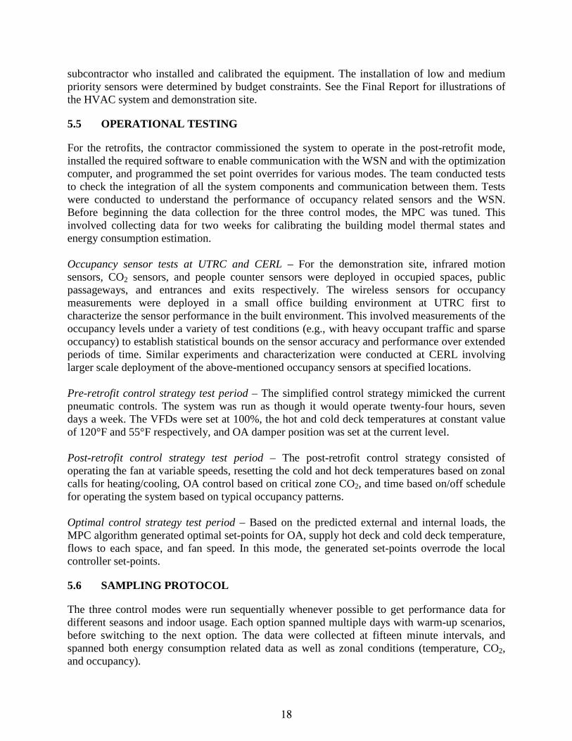
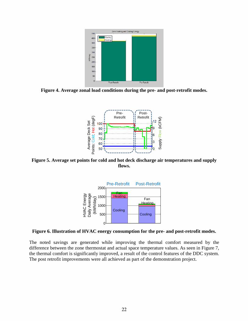
To ensure consistent comparisons between the energy consumption levels for the two modes, they were implemented sequentially in July 2011 as follows: pre-retrofit mode during July 16–31, and post-retrofit mode during July 5–13. The similarity between the ambient and usage conditions for the two modes made it possible to directly compare measured BTU and electrical meter energy consumption without additional normalization or averaging. Although this was possible, it may have introduced sources of errors, as is the case with any model. Based on direct comparison of electrical and thermal energy consumption, as illustrated in Figure 6, one concludes that the relative energy consumption savings are nearly 30%. These are direct results of three improvements to the post-retrofitted system operation:

• Schedule: as opposed to the pre-retrofitted system that operates at constant volume and schedule at all times, the post-retrofitted system has been scheduled to operate only during working hours with additional pre-cooling and heating. Outside the normal working hours, the occupants have the possibility to override the otherwise scheduled set points by selecting appropriate input of the thermostat.

• Set point schedules: as opposed to the pre-retrofit scheduled fixed set points for all weather and load conditions, the post-retrofit schedule uses heuristics to adapt these values. These differences are partly illustrated in Figure 5, where it can be observed that the pre-retrofit mode saves energy by using lower hot deck discharge air temperature and lower supply flow. Evidently, the pre-retrofit control mode conservatively utilized higher hot deck temperatures and lower cold deck temperatures, and much higher supply airflow rates.

• Local control: the local controllers are improved by using features beyond the capabilities of the original pneumatic-based controllers (such as the integral action of the DDC’s proportional-integral (PI) control algorithm, economizer, and temperature and pressure resets).

22

Figure 4. Average zonal load conditions during the pre- and post-retrofit modes.

Figure 5. Average set points for cold and hot deck discharge air temperatures and supply

flows.

Figure 6. Illustration of HVAC energy consumption for the pre- and post-retrofit modes.

The noted savings are generated while improving the thermal comfort measured by the difference between the zone thermostat and actual space temperature values. As seen in Figure 7, the thermal comfort is significantly improved, a result of the control features of the DDC system. The post retrofit improvements were all achieved as part of the demonstration project.

Ave

rage

Dec

k S

et

Poi

nts:

Col

d;H

ot (

degF

)

S

uppl

y F

low

(kC

FM

)

Pre-Retrofit

Post-Retrofit

Pre-Retrofit

HV

AC

Ene

rgy

Dai

ly A

vera

ge

(kW

h/da

y )

Post-Retrofit

0

500

1000

1500

2000

Fan

FanHeating

Heating

CoolingCooling

23

Figure 7. Average difference between set points and actual space temperature values for

pre- and post-retrofit.

6.2 PERFORMANCE COMPARISON BETWEEN POST-RETROFIT AND OPTIMIZATION MODES

This section summarizes the performance benefits of the optimized system controlled with set points generated by the model-based predictive algorithm. The main challenge in estimating these benefits was the variations in ambient and usage conditions between these two modes. To minimize this challenge we used data between days when the ambient conditions were similar. Therefore, for each day when the MPC algorithm was executed, a set of days were identified when the post-retrofit mode was executed and when the ambient temperature had a similar pattern. Figure 8 shows energy savings achieved by MPC, and peak power consumption data for the MPC and post-retrofit modes respectively; these were recorded for the MPC data, from Thursday, October 27, 2011, and for post-retrofit data, from Monday, October 31, 2011. The data illustrated in these figures were used to generate the overall estimates of Table 1. An analysis of these plots illustrates the following:

• The maximum thermostat set point tracking error is 1°F for the MPC mode and 0.5°F for the post-retrofit mode. This is a result of the flexibility of the MPC algorithm and its optimality. The designer can select the acceptable range of the thermal comfort and define bounds around the thermostat set points. The MPC algorithm generated space temperature levels that were close to the acceptable bounds of the thermal comfort range.

• Although energy was saved for the MPC mode, the peak power increased. This was because the thermostat set point for the largest zone was changed at 9:00 AM, while the MPC algorithm tried to control the temperature within the new thermal comfort range.

• The space temperature for the MPC mode had higher frequency oscillations than for the post-retrofit mode. This can be explained by: (i) model errors: the MPC uses models for predictions that trigger the system to compensate; (ii) the local control transient behavior is not included in the supervisory controller. We assumed that the local controller responded consistently fast and accurately. But after several experiments, this assumption proved false.

Set

Poi

nt

Tra

ckin

g E

rror

(O

ccup

ied

Tim

e)

(deg

F)

Zone 1 Zone 2 Zone 3 Zone 4 Zone 501234

Zone 1 Zone 2 Zone 3 Zone 4 Zone 501234

Pre-Retrofit

Post-Retrofit

24

To minimize the impact of variations in ambient conditions on performance benefit estimation, the MPC data was compared against multiple post-retrofit datasets when ambient temperature patterns were similar. The data are summarized here and described in detail in the Final Report. Positive entries in shaded columns titled “relative energy savings” and “relative peak power decrease” indicate reductions, whereas negative entries indicate increase for MPC mode. Despite efforts to ensure consistency in indoor and ambient conditions, there is variability in energy savings estimates. However, average energy savings are evident in every case, providing consistent reductions of 11-64% relative to the post-retrofit mode; the average savings were estimated by comparing the average baseline energy consumption with that for the MPC case in each case (also denoted as Test #). With two exceptions (see MPC Test #3 case), the peak power for the MPC mode is higher than for the post-retrofit mode. This was a direct consequence of the controlled system (oscillation) behavior. Figure 8 summarizes the average energy savings for the cases summarized in the Final Report, as well as the peak power usage average.

Figure 8. Summary of HVAC system energy use (top) and peak power consumption

(bottom) for 2011 demonstration tests.

25

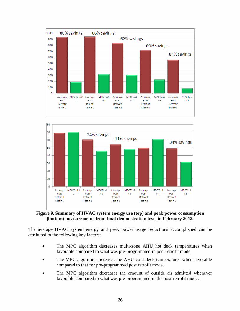
Using the insights gained from the 2011 demonstration data, the MPC algorithm was revised and improved, including refined dynamical models for the mixing, hot deck, and cold deck temperatures, to improve peak power usage performance for the MPC mode. Another set of experiments was conducted during the week of February 13-17, 2012. For each MPC case (a day when the MPC algorithm was executed during the occupied hours), a number of similar ambient-temperature days were identified when the post-retrofit algorithm was implemented. The corresponding performance metrics (energy consumption and peak power) are summarized in Figure 14 and described in detail in the Final Report. The following conclusions were drawn:

• Energy consumption for the HVAC system was reduced from 60-85%, relative to post-retrofit mode levels. These significantly exceed the 15% demonstration target metric.

• For three cases, peak power usage was reduced from 10-35%. These values are also above the 10% target.

• For two cases, peak power usage increased by 1% and 22%, which was below the performance target. For MPC Test #1 on February 13, 2012, when peak power increased by 1%, the 70kW power demand occurred early in the morning when the HVAC system was started. That exception aside, all other power generated is below 50kW for the post retrofit mode. This initial peak could be decreased by adjusting the trade-offs between average energy use and peak power; for example the HVAC system could be started earlier. In this case the average energy consumption could be increased slightly (still remaining above the 15% target). A similar pattern is observed for MPC Test #4 on February 16, 2012, when the peak power increased to 61kW early in the morning while it remained below 38kW for the rest of the day. This again is due to an over-reaction of the MPC algorithm to the out-of-comfort-range temperature values reached while the HVAC system was shut down during the night.

Figure 9 summarizes the average energy savings for all the cases, as well as the peak power usage average.

26

Figure 9. Summary of HVAC system energy use (top) and peak power consumption

(bottom) measurements from final demonstration tests in February 2012. The average HVAC system energy and peak power usage reductions accomplished can be attributed to the following key factors:

• The MPC algorithm decreases multi-zone AHU hot deck temperatures when favorable compared to what was pre-programmed in post retrofit mode.

• The MPC algorithm increases the AHU cold deck temperatures when favorable compared to that for pre-programmed post retrofit mode.

• The MPC algorithm decreases the amount of outside air admitted whenever favorable compared to what was pre-programmed in the post-retrofit mode.

27

The MPC algorithm accomplishes these reductions on a dynamic basis, via 15 minute updates. Figure 10 illustrates the resulting daily average of the hot and cold deck temperatures and system variables for the post-retrofit mode and for the MPC mode of operation. All (energy) relevant system variables were manipulated in a favorable direction. This explains the substantial energy use reductions accomplished. The deck temperatures achieved for the pre-retrofit (pneumatic) controls are also illustrated for reference (see red and blue lines), supporting the large reductions in energy use accomplished when moving from pneumatic to DDC controls. Dual deck systems (prevalent in older buildings) are likely more prone to energy waste from system duct losses and leakages, compared to single deck HVAC systems (which are deployed more commonly now). Thus, the impact of a higher difference between the heating and cooling deck temperature in driving energy use is likely more obvious for dual deck systems. Finally, a more fine tuned DDC mode control strategy involving reset of the cooling and heating deck set points based on outside weather, rather than a seasonal setting would have captured some of the savings achieved by the MPC scheme. More detailed assessments and analysis for different variants of the central HVAC system and of baseline DDC mode control approaches are needed to ascertain the variability in the energy use and peak power reduction benefits across DoD stock.

Figure 10. Summary for the post retrofit and MPC modes, from demonstration tests in

February 2012, illustrating the system operation changes accomplished by the optimization algorithm.

Figure 11 illustrates the indoor comfort metrics for zonal temperature tracking and CO2 levels, showing that the controlled space temperatures never deviate beyond ±1°F of the temperature set point (TSP), and are within the CO2 level limit (derived from ASHRAE 62.1) with the exception of one case where the constraint is violated.

28

Figure 11. Summary for the post retrofit and MPC modes, from demonstration tests in

February 2012, illustrating the MPC performance in tracking occupant space temperature relative to zone set point TSP during occupied hours (left) and maintaining indoor CO2

levels (right).

29

7.0 COST ASSESSMENT

The demonstration quantified operational cost reductions due to energy efficiency gains as well as installed (first) cost and maintenance cost reductions from using WSN and MPC for building HVAC control retrofits. The average life of DDC is about twenty five years [15] so a twenty-five year time frame for the life-cycle cost estimate was used.

7.1 COST MODEL

Table 4. Cost model for wireless sensor network.

Cost Element Data Tracked During the

Demonstration Estimated Costs

Hardware and software capital costs

Estimates made based on component costs of Wireless sensors and related network infrastructure for demonstration and software for controls platform

$53,895

Installation costs Labor and material required to install sensors and controls platform

$19,122

Consumables

Estimates based on rate of consumable use during the field demonstration including batteries, networking cables, etc.

No consumables for the MPC installation

Facility operational costs

Reduction in energy consumption based on additional sensing relative to the baseline data

Pre-retrofit to post-retrofit: $8645 (57.7% savings) Pre-retrofit to MPC: $9640 (63.2% savings)

Maintenance

• Frequency of required maintenance for WSN and controls platform

• Labor and material per maintenance action

• 2 hours average per month to attend to control configuration management and network diagnostics

• Labor of the BAS technician/facility technician is $2225 per year and ideally no material cost involved in maintenance for this deployment

Hardware lifetime

Estimation of the life-cycle cost based on the equipment degradation, configuration management, and labor associated with the WSN hardware

The equipment used in this deployment does not have attributes that contribute to the life-cycle cost. The components used for the demo have a long lifetime up to twenty-five years with minimal degradation (wireless sensors, DDC boxes, etc.).

Operator training

Estimate of training costs for facility personnel on usage of the equipment and operational adjustments to both WSN and controls algorithm

• The interface for the operator is similar to the existing interface and does not require special training for use.

• Sequence of operations for post-retrofit controls is already documented and provided. Post-retrofit operator training has already happened.

• Training for advanced algorithms was not provided since decision was made to discontinue the advanced control platform.

• Hardware capital costs: This estimate is based on the component costs of the

WSN system and compared with the hardware cost of a similar wired networking

30

system. Cost of an additional sensor was quantified to demonstrate the cost feasibility of scaling the network with additional sensors. Additional computer requirements, if any, for WSN and MPC compared to computer requirements for a BMS system, are also included.

• Installation costs: This estimate is based on the cost involved in installing and commissioning the WSN system. WSN uses a self-configuring routing protocol reducing the cost of the additional sensor installation as the number of sensors increases as opposed to a wired network.

• Consumables: This estimate is based on identifying the consumable equipment during the demonstration period and its impact on the operational efficiency of the system.

• Facility operational costs: This estimate is based on the measured electric energy consumption (KWh) and cooling/heating energy consumption (MMBtu/hr) after the installation of the technology (for optimal control strategy) and before the installation (baseline).

• Maintenance: This estimate includes the cost of each maintenance action including labor and hardware supplies.

• Hardware lifetime: A life-cycle cost of using WSN was estimated based on the maintenance requirement, equipment degradation, configuration management, and labor associated with the use of WSN for HVAC control.

• Operator training: This estimate includes the cost of the facility operation personnel training for using WSN and MPC.

7.2 COST DRIVERS

The project addresses three important drivers:

1. Regulatory Driver: EPACT of 1992, EISA of 2007 (Title IV, Subtitle C), and EO 13423 mandate DoD to improve facility energy efficiency by 30% beyond 2003 levels.

2. Technology Driver: Retro-commissioning advanced controls in existing old buildings to optimize the performance of the HVAC and building systems requires significant investments. Through this project we demonstrated the use of easy to retrofit wireless sensors to enable low footprint supervisory controllers based on existing systems and controls to improve energy efficiency. Recent advances in buildings automation and wireless technologies have fueled this deployment.

3. Economic Driver: Key to retro-commissioning in existing buildings is to understand the return-on-investment. This project demonstrated a two-fold advantage: 1) demonstration of significant energy savings using advanced sensing and control (60% or more energy demand reduction); and 2) identification of the persistent unnoticed faults during the retro-commissioning process (e.g., identification of stuck dampers).

31

This technology is applicable to existing buildings with sub-optimal controls and those that are not served by a BAS. Buildings that are not served by digital controls provide the best opportunity for deploying the technology. While climate zones with distinct four seasons will benefit most from the technology, but buildings in other climate zones can also benefit. Buildings with existing automation need careful interoperability considerations for deploying this technology. This technology can be applied to typical commercial buildings served by packaged RTUs or built-up systems.

7.3 COST ANALYSIS AND COMPARISON

DoD can realize improved building automation in three phases:

1. Asset visibility: Advanced low-cost sensors improved the operational visibility of the assets within energy related systems.

2. Process visibility: Retrofit energy management platforms provide improved operational envelope of the systems due to increased visibility into the process like occupancy-based HVAC systems and demand-controlled ventilation.

3. Enterprise visibility: This technology is repeatable across multiple DoD facilities providing opportunities to integrate data and visualize energy usage across facilities in a unified fashion. Among the 250,000 to 300,000 DoD buildings, at least 32,000 are equipped with variable area volume unit systems for HVAC, for which this technology is readily applicable. The realizable energy savings would vary across different climates, and variants of central HVAC systems. For the remainder, which are likely comprised of buildings served by unitary systems (e.g., packaged RTUs) the technology demonstrated can also be extended, but the building served by packaged terminal units and variable refrigerant volume systems, the technology is not applicable in its current form.

The demonstration project realized the following conclusions:

• Novel control methods for operating buildings based on occupancy patterns and buildings usage has significant potential for energy demand reduction.

• Low-cost wireless sensors improve observability and controllability of existing buildings.

• Improved human-machine interfaces (HMI) provide asset and process visibility reducing time to failure detection and reducing unattended energy losses.

A life-cycle cost (LCC) analysis was performed using the National Institute of Standards and Technology (NIST) Building Life-Cycle Cost (BLCC) program. Three distinct scenarios were developed during this analysis: Scenario 1: This includes the total investment in the MPC hardware and installation and demonstrated energy savings based on the current utility costs in the area.

32

Scenario 2: The hardware cost is discounted to reflect the real installation in a typical facility – the cost of BTU meters is reduced from $12,800 per unit to $2000 per unit since significant cost is in the installation specific to the facility. Discussions with the contractor suggested this improvement for typical installation where commercial off-the-shelf (COTS) devices can be used without sacrificing performance measurement fidelity required for implementation. Scenario 3: The BTU meters are eliminated assuming the algorithm can be run with existing meters or using the raw data from the balancer along with a software program to estimate energy. Scenario 4: The electricity rates are doubled to reflect the electricity costs in other parts of the U.S compared to Chicago, IL. COTS devices as in Scenario 2 are used in this estimation. The savings to investment ratio and payback are summarized in Table 5. These values are highly dependent on hardware costs for installation. Cost effective BTU metering using COTS hardware or advanced analytics based on raw data from the balancer can reduce payback period.

Table 5. Post-retrofit to MPC comparison for four scenarios.

Attribute Scenario 1 Scenario 2 Scenario 3 Scenario 4 Study period 20 years 20 years 20 years 20 years Capital – post-retrofit $0 $0 $0 $0 Capital – MPC $52,856 $31,256 $27,256 $31,256 Energy cost – post-retrofit $95,043 $95,043 $95,043 $190,085 Energy cost – MPC $46,823 $46,823 $46,823 $93,646 Energy savings with MPC $48,220 $48,220 $48,220 $96,440 Present value LCC – post-retrofit $130,061 $130,061 $130,061 $225,103 Present value LCC – MPC $134,697 $113,097 $109,097 $159,920 Net savings -$4636 $16,964 $20,964 $65,184 Savings-to-investment ratio 0.91 1.54 1.77 3.09 Adjusted internal rate of return N/A 4.64% 5.36% 8.34% Payback period – simple 18 11 10 6 Payback period - discounted N/A 13 11 6

Ubiquitous sensing improves observability and controllability of building systems. This project demonstrated that standards-based sensing and control integration to existing buildings will drive down costs by inviting “non-traditional suppliers” into the market by increasing size of the market and potentially improving competition and rate of innovation. This requires end-users to support early adoption of standards-based approaches. This project is intended to replace traditional wired communications and deploy advanced supervisory control. Table 6 shows the comparison between wired and wireless systems for the same site selection. Wireless sensors provided 11% savings in the procurement and installation.

33

Table 6. Wired versus wireless comparison.

Component Wired ($) Wireless ($) Sensor & materials* 20,951.65 10,062.50 Wiring 13,948.35 1414.50 Wireless equipment 0.00 12,357.00 Labor# 126,189.00 119,445.00 Total 161,089.00 143,279.00

*Sensors that were replaced with wireless are counted toward this component. Cost of common components that would exist in both the installations is excluded. #Labor costs reflect total project labor costs as integrated number of hours in various stages of labor changes based on the configuration.

The following considerations have to be made in interpreting Table 7:

• The comparison does not take into account the cost of the original LonWorks network installation. This assumes the exclusion of baseline infrastructure costs for the wired system.

• The installation of the wireless infrastructure is a one-time cost and incremental installation of the sensors has near zero labor and installation costs. Additional wireless points on the network (up to 150 points) is $120 for this installation (excluding sensor). Additional wired points on the network would between $400 and $900 depending on the installation location and labor involved. Figure 12 shows the growth of the network cost for comparable wired and wireless systems. Figure 13 shows the cost savings of wireless compared to wired as the network size grows.

• The location of the wireless sensor is not constrained, as is the case of the wired installation, thereby providing optimal observable locations for energy-efficient control.

Figure 12. Comparison of wired versus wireless as network size increases.

34

Figure 13. Cost savings using wireless as network size increases.

We estimated the cost of repeating the functionality in an operational environment at 40-50% lower than the current estimate as shown in Table 7. The primary reason is the integration expertise gained as part of the first deployment. Repeating similar installation in multiple DoD sites lowers the cost significantly benefiting from ease of placement for wireless sensors.

35

8.0 IMPLEMENTATION ISSUES

The project met significant implementation challenges that were resolved but resulted in delays and, ultimately, a smaller data set than originally planned. These challenges ranged from sensor issues to network communication issues. Related to the sensor issues, there were limited sets of data for which water-to-air enthalpy balance did not hold and an explanation could not be found. This was not resolved even after additional recalibration was made including sensor re-placement, and installation of averaging sensors. These calibration and validation issues are expected to occur for other systems, too. People counter sensors generated data that occasionally yielded large accumulation errors which could only be explained by the well-known sensor technology issues. Network communication issues were relatively small. Twice there were issues with the on-board electronics of a wireless sensor that was replaced each time. In view of the large number of wireless sensors installed as part of the project, this was considered to be a minor malfunction. On several occasions the communication between the optimization platform and the BAS server was interrupted. Although this was improved by changing some of the communication protocol parameters these communication issues continued with a smaller frequency. As a result, some of the experimental test data was compromised and was not included in the data processing effort. An additional challenge was posed by the small set of options available for communication between an advanced optimization platform and a BAS. A significantly large effort, larger than originally envisioned, was made to make communication between these platforms possible. The software toolchain for bi-directional communication and for overriding BAS set points in a consistent manner is relatively complex and not readily implemented at large-scale. The on-line data communicated between the two computers was relatively small for this project, but is expected to be significantly more challenging for a set of building HVAC units.

37

9.0 REFERENCES

http://www.eia.doe.gov/emeu/cbecs/cbecs2003/detailed_tables_2003/detailed_tables_2003.html

Energy Impact of Commercial Building Controls and Performance Diagnostics: Market Characterization, Energy Impact of Building Faults and the Energy Savings Potential, TIAX Report D0180, for U.S. DOE Contract 030400101, Nov 2005.

http://www.cecer.army.mil/

Elmahdy, A. H.; Beattie, D. G.; Direct Digital Control of Small and Medium-Size Buildings; Division of Building Research, National Research Council of Canada, 1981

ASHRAE Guideline 14-2002, Measurement of energy and demand savings.

ASHRAE: Service Life and Maintenance Cost Database; http://xp20.ashrae.org/publicdatabase/default.asp

Henze, G., Dodier, R., Krarti, M., Development of a Predictive Optimal Controller for Thermal Energy Storage Systems, International Journal of Heating, Ventilating, Air-Conditioning and Refrigerating Research, 1996.

A-1

APPENDIX A

POINTS OF CONTACT

Point of Contact Organization

Phone Fax

E-Mail Role In Project

Satish Narayanan United Technologies Research Center 411 Silver Lane MS 129-13 East Hartford, CT 06118

Phone: 860-610-7412 Fax: 860-660-1291 E-Mail: [email protected]

Principal Investigator (PI)

Teja Kuruganti Oak Ridge National Laboratory, Extreme Measurement Communications Center (EMC2) 1 Bethel Valley Road MS-6085 Oak Ridge, TN 37831


Co-PI

Francesco Borrelli University of California at Berkeley Department of Mechanical Engineering 5132 Etcheverry Hall Mailstop 1740 Berkeley, CA 94720-1740


Co-PI

David M. Schwenk U.S. Army Corps of Engineers ERDC-CERL 2902 Newmark Drive Champaign, IL 61822


DoD liaison at the demo site

James Galvin ESTCP 4800 Mark Center Drive Suite 17D08 Alexandria, VA 22350-3605

Phone : 571-372-6397 E-Mail : [email protected]

Energy and Water Program Manager

ESTCP Office4800 Mark Center DriveSuite 17D08Alexandria, VA 22350-3605

(571) 372-6565 (Phone)

E-mail: [email protected]

estcp cost and performance report - defense … and abbreviations (continued) vi pir...

Documents