estimating chlorophyll a concentrations of several …

ESTIMATING CHLOROPHYLL A CONCENTRATIONS OF SEVERAL INLAND WATERSWITH HYPERSPECTRAL DATA AND MACHINE LEARNING MODELS

P. M. Maier1, S. Keller1

1 Karlsruhe Institute of Technology (KIT), Institute of Photogrammetry and Remote Sensing,Englerstr. 7, D-76131 Karlsruhe, Germany

(philipp.maier, sina.keller)@kit.edu

Commission I,WG I/1

KEY WORDS: Spectral Resolution, Inland Waters, Supervised Learning, Support Vector Machine, Random Forest, Neural Network,Remote Sensing, Phytoplankton

ABSTRACT:

Water is a key component of life, the natural environment and human health. For monitoring the conditions of a water body, thechlorophyll a concentration can serve as a proxy for nutrients and oxygen supply. In situ measurements of water quality parameters areoften time-consuming, expensive and limited in areal validity. Therefore, we apply remote sensing techniques. During field campaigns,we collected hyperspectral data with a spectrometer and in situ measured chlorophyll a concentrations of 13 inland water bodies withdifferent spectral characteristics. One objective of this study is to estimate chlorophyll a concentrations of these inland waters by applyingthree machine learning regression models: Random Forest, Support Vector Machine and an Artificial Neural Network. Additionally,we simulate four different hyperspectral resolutions of the spectrometer data to investigate the effects on the estimation performance.Furthermore, the application of first order derivatives of the spectra is evaluated in turn to the regression performance. This study revealsthe potential of combining machine learning approaches and remote sensing data for inland waters. Each machine learning modelachieves an R2-score between 80 % to 90 % for the regression on chlorophyll a concentrations. The random forest model benefits clearlyfrom the applied derivatives of the spectra. In further studies, we will focus on the application of machine learning models on spectralsatellite data to enhance the area-wide estimation of chlorophyll a concentration for inland waters.

1. INTRODUCTION

Clean and fresh water is a key resource for the environment andhuman health. Water quality, however, is threatened by over-fertilization leading to algal blooms, oxygen deficiency and hence,mass death of fish. Furthermore, some phytoplankton species,especially blue-green algae, can be harmful for humans. Forexample, they might spread into drinking water reservoirs andrelease toxic substances. To overview and assess the dangerouseffects of such algal blooms, a continuous monitoring of the algaegrowth is advisable.

The feasibility of conventional in-situ monitoring approaches isrestricted due to their limitations of both spatial coverage andtemporal frequency of the recording. As a consequence, we ap-prove and follow the remote sensing approach which is alreadyused for monitoring chlorophyll a concentration in water sincethe 1990s (Gitelson, 1992). Data recorded by remote sensingtechniques e.g. satellites is used successfully in the context ofestimating chlorophyll a concentration in ocean waters e.g. byO’Reilly et al. (1998). Regarding inland waters, this estimationseems to be more challenging (Palmer et al., 2015). The availablemultispectral satellite data is primarily useful for observing oceanwater or land surface. For monitoring small water bodies, thespatial resolution of satellite images is often too low. The same ap-plies for the spectral resolution, which is rather insufficient for e.g.estimating phytoplankton pigments based on satellite data (Palmeret al., 2015). In addition, inland waters are optically more complexthan ocean waters because of various suspended particles (Hunteret al., 2008). Thus the transferability of the estimation model isnot ensured.

The relation between algae existence and remote sensing is pri-marily linked to the absorption of light in a wavelength of 665 nmon the pigment chlorophyll a (Morel and Prieur, 1977). This re-flection minimum and the following reflection maximum around700 nm serve as the basic wavelengths of the band ratio approachesfor the identification of chlorophyll a in inland waters. Ratioapproaches are often used by e.g. Gitelson (1992); Schalles etal. (1998); Gons (1999); Dall’Olmo et al. (2003); Gitelson et al.(2007); Zhou et al. (2013). Schalles et al. (1998) rely on thearea under the peak around 700 nm or just the respective ampli-tude for the estimation of chlorophyll a concentration. Alterna-tively, derivatives of the spectra are applied in this context aswell (Rundquist, 1996).

Another approach for the estimation of water parameters by hy-perspectral data are data-driven machine learning models primarybased on supervised learning. For supervised learning, a dataset isdivided into sets where e.g. one set is used for the training of themodel and the other set is employed to evaluate the model. Thepotential of these machine learning models for the estimation ofseveral water parameters is shown in the context of coastal watersby e.g. Keiner and Yan (1998); Gonzlez Vilas et al. (2011); Kim etal. (2014), in the context of rivers by Maier et al. (2018) and Kelleret al. (2018) as well as for big lakes by Odermatt et al. (2010).

For the recording of the remote sensing data a multitude of differ-ent sensor techniques are applied: spectrometers, hyperspectralcameras and satellite data. They vary widely with respect to thespatial and spectral resolution. Satellite data offers many advan-tages: the temporal repetition rate is constant, they can cover hugeareas and in the long run it is a cost-effective solution. However,the large pixel size might be adverse for small inland waters and

ISPRS Annals of the Photogrammetry, Remote Sensing and Spatial Information Sciences, Volume IV-2/W5, 2019 ISPRS Geospatial Week 2019, 10–14 June 2019, Enschede, The Netherlands

This contribution has been peer-reviewed. The double-blind peer-review was conducted on the basis of the full paper. https://doi.org/10.5194/isprs-annals-IV-2-W5-609-2019 | © Authors 2019. CC BY 4.0 License.

609

the spectral bandwidth is often too coarse. Decker et al. (1992) an-alyzed the compatibility of the Landsat TM sensor and the SPOTsensor to the chlorophyll a absorption. Neither of the sensorscover the range between 690 nm and 760 nm, so the peak around700 nm related to chlorophyll a cannot be detected. Then again,push broom sensors with narrow bandwidths of 10 nm to 20 nm be-tween 600 nm to 720 nm seem to be practicable for the estimationof phytoplankton substances (Decker et al., 1992). With the launchof the DESIS (DLR Earth Sensing Imaging Spectrometer) missionin 2018 and the upcoming launch of EnMAP (Environmental Map-ping and Anlaysis Program), monitoring of inland waters withreasonable spatial extent and hyperspectral resolution should befeasible. Up to now, unmanned aerial vehicles (UAVs) provide anappropriate spectral and spatial resolution for any remote sensingbased monitoring approach over limited areas.

In this study, we assess the transferability of applied machinelearning models for the estimation of chlorophyll a concentra-tions with hyperspectral data and for several inland water bodies.Therefore, we recorded our own hyperspectral dataset in severalfield campaigns with a spectrometer1 from 13 different inlandwaters. As reference data, we collected water samples, whichwere evaluated with a photometer2 regarding their chlorophyll aconcentration. Finally, the dataset for this study contains of 422datapoints including hyperspectral data and reference data. For theestimation of chlorophyll a concentration, we apply three differentregression models: Random Forest (RF), Support Vector Machine(SVM) and an Artificial Neural Network (ANN). An importantfactor for the estimation performance of a model is the spectralresolution of the sensor. As we rely on a dataset collected witha spectrometer, we aggregate the spectra to several bands withdifferent resolutions to simulate hyperspectral cameras or satellitesensors. After various pre-tests, we decided to apply four differentresolutions with a continuous interval of 4 nm, 8 nm, 12 nm and20 nm. Additionally, we calculated derivatives of the differentaggregated data and applied the same regression models.

The objectives of this study are:

• to describe the recorded dataset including the measurementsetup of our field campaigns,

• to demonstrate the potential of supervised learning modelsfor the estimation of chlorophyll a concentration of differentinland waters,

• to assess the spectral resolution in the context of estimatingchlorophyll a concentration as well as to determine, whichbandwidths are suitable to achieve a sufficient regressionperformance,

• to measure the effects of using derivatives of a spectrum toestimate chlorophyll a concentrations and

• finally to evaluate the different machine learning models.

We describe the applied sensor systems of the field campaigns andthe measured dataset in Section 2. In Section 3, the presentationof the machine learning models follows. Section 4 contains theevaluation of the measured dataset and the assessment of thedifferent approaches. Finally, we conclude our studies in Section 5and give an overview about future research application based onthe presented dataset.

1JB Hyperspectral Devices UG, Germany2AlgaeLabAnalyser bbe moldaenke GmbH, Germany

2. SENSORS AND DATASET

To reveal the potential of supervised learning models for the esti-mation of chlorophyll a concentrations in different inland waters,many data of such waters as well as varying chlorophyll a concen-trations are needed. The presented dataset consists of hyperspec-tral data and chlorophyll a concentrations. Both types of data aremeasured with two different sensor systems. The recordings werechallenging, since we needed to produce comparable hyperspec-tral data with varying daytime over a measurement period of fourmonths.

2.1 Sensors and Data Acquisition

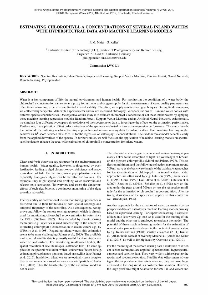
Figure 1. Measurement setup of the RoX spectrometer at anartificial pond.

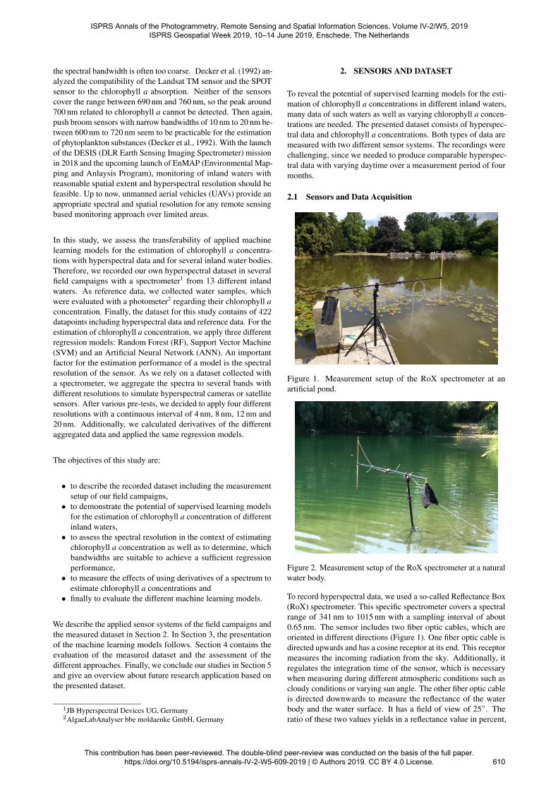
Figure 2. Measurement setup of the RoX spectrometer at a naturalwater body.

To record hyperspectral data, we used a so-called Reflectance Box(RoX) spectrometer. This specific spectrometer covers a spectralrange of 341 nm to 1015 nm with a sampling interval of about0.65 nm. The sensor includes two fiber optic cables, which areoriented in different directions (Figure 1). One fiber optic cable isdirected upwards and has a cosine receptor at its end. This receptormeasures the incoming radiation from the sky. Additionally, itregulates the integration time of the sensor, which is necessarywhen measuring during different atmospheric conditions such ascloudy conditions or varying sun angle. The other fiber optic cableis directed downwards to measure the reflectance of the waterbody and the water surface. It has a field of view of 25◦. Theratio of these two values yields in a reflectance value in percent,



610

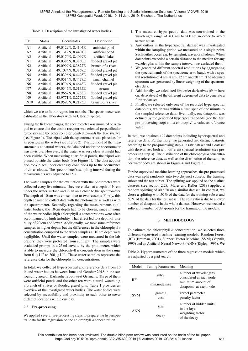
Table 1. Description of the investigated water bodies.

ID Status Coordinates Description

A1 Artificial 49.0129N, 8.4104E artificial pondA2 Artificial 49.1312N, 8.4401E artificial pondA3 Artificial 49.0170N, 8.4049E artificial lakeN1 Artificial 49.0385N, 8.3850E flooded gravel pitN2 Artificial 49.0999N, 8.3822E branch of a riverN3 Artificial 49.1074N, 8.3867E flooded gravel pitN4 Artificial 49.0396N, 8.4498E flooded gravel pitN5 Artificial 49.0514N, 8.4477E small channelN6 Artificial 49.0794N, 8.4648E flooded gravel pitN7 Artificial 49.0345N, 8.3135E streamN8 Artificial 48.9667N, 8.3288E flooded gravel pitN9 Artificial 48.9771N, 8.2724E flooded gravel pitN10 Artificial 48.9590N, 8.2193E branch of a river

which we use to fit our regression models. The spectrometer wascalibrated in the laboratory with an Ulbricht sphere.

During the field campaigns, the spectrometer was mounted on a tri-pod to ensure that the cosine receptor was oriented perpendicularto the sky and the other receptor pointed towards the lake surface(see Figure 1). The tripod with the spectrometer was placed as faras possible in the water (see Figure 2). During most of the mea-surements at natural waters, the lake bed under the spectrometerwas invisible. However, if the water was very clear, it might hadbeen visible. When measuring at artificial ponds, the tripod wasplaced outside the water body (see Figure 1). The data acquisi-tion took place under clear sky conditions up to the occurrenceof cirrus clouds. The spectrometer’s sampling interval during themeasurements was adjusted to 15 s.

The water samples for the evaluation with the photometer werecollected every five minutes. They were taken at a depth of 10 cmunder the water surface and in an area close to the spectrometer.The depth of 10 cm was chosen due to two reasons: Firstly, thisdepth ensured to collect data with the photometer as well as withthe spectrometer. Secondly, regarding the measurements at allwater bodies, the 10 cm depth had to be chosen, since in someof the water bodies high chlorophyll a concentrations were oftenaccompanied by high turbidity. That effect led to a depth of visi-bility of 20 cm and lower. Additionally, we took some referencesamples in higher depths but the differences in the chlorophyll aconcentration compared to the water samples at 10 cm depth werenegligible. Until the water samples were measured in the lab-oratory, they were protected from sunlight. The samples wereevaluated prompt in a 25 ml cuvette by the photometer, whichis able to measure the chlorophyll a concentration in the rangefrom 0 µg L−1 to 200 µg L−1. These water samples represent thereference data for the chlorophyll a concentrations.

In total, we collected hyperspectral and reference data from 13inland water bodies between June and October 2018 in the sur-rounding area of Karlsruhe, Southwest Germany. Three of themwere artificial ponds and the other ten were natural waters e.g.a branch of a river or flooded gravel pits. Table 1 provides anoverview of the investigated water bodies. The water bodies wereselected by accessibility and proximity to each other to coverdifferent locations within one day.

2.2 Pre-processing

We applied several pre-processing steps to prepare the hyperspec-tral data for the regression on the chlorophyll a concentration.

1. The measured hyperspectral data was constrained to thewavelength range of 400 nm to 900 nm in order to avoidsensor noise.

2. Any outlier in the hyperspectral dataset was investigatedwithin the sampling period we measured on a single point.Such outlier occur e.g. by sun glint, waves or shadows. Whendatapoints exceeded a certain distance to the median for anywavelengths within the sample interval, we excluded them.

3. We generated different spectral resolutions by aggregatingthe spectral bands of the spectrometer to bands with a spec-tral resolution of 4 nm, 8 nm, 12 nm and 20 nm. The obtainedspectrum was generated by linear weighting of the spectrom-eter data.

4. Additionally, we calculated first order derivatives (from hereon: derivatives) of the different aggregated data to generate afurther dataset.

5. Finally, we selected only one of the recorded hyperspectraldatapoints, which was within a time span of one minute tothe sampled reference data. Eventually, one datapoint wasdefined by the generated hyperspectral bands (see the firstpre-processing step) and a chlorophyll a value as referencevalue.

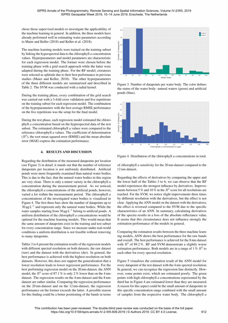
In total, we obtained 422 datapoints including hyperspectral andreference data. Furthermore, we generated two distinct datasetsaccording to the pre-processing step 4: a raw dataset and a datasetwith derivatives, both with different spectral resolutions (see pre-processing step 3). The distribution of the chlorophyll a concentra-tion, the reference data, as well as the distribution of the samplesper water body are shown in Figure 4 and Figure 3.

For the supervised machine learning approaches, the pre-processeddata was split randomly into two disjunct subsets: the trainingsubset and the test subset. The splitting was applied on the distinctdatasets (see section 2.2). Maier and Keller (2018) applied arandom splitting of 30 : 70 on a similar dataset. In contrast, wechose a splitting with 50 % of the data for the training subset and50 % of the data for the test subset. The split ratio is due to a lowernumber of datapoints in the whole dataset. However, we needed asufficient number of datapoints for the training of the models.

3. METHODOLOGY

To estimate the chlorophyll a concentration, we selected threedifferent supervised machine learning models: Random Forest(RF) (Breiman, 2001), Support Vector Machine (SVM) (Vapnik,1995) and an Artificial Neural Network (ANN) (Ripley, 1996). We

Table 2. Hyperparameters of the three regression models whichare adjusted by a grid search.

Model Tuning Parameters Meaning

RFmtry

number of wavelengthsconsidered at each node

min.node.sizeminimum amount ofdatapoints at each node

SVMgamma kernel parameter

cost penalty factor

ANNsize

number of hidden unitsin the layer

decayweighting factorof the decay



611

chose those supervised models to investigate the applicability ofthe machine learning in general. In addition, the three models havealready performed well in estimating water parameters accordingto Maier and Keller (2018) and Keller et al. (2018).

The machine learning models were trained on the training subsetby linking the hyperspectral data to the chlorophyll a concentrationvalues. Hyperparameters and model parameters are characteristicfor each regression model. The former were chosen before thetraining phase with a grid search approach while the latter wereadapted during the training phase. For the RF model, extratreeswere selected as splitrule due to their best performance in previousstudies (Maier and Keller, 2018). The other hyperparametersof the three different models are summarized and described inTable 2. The SVM was conducted with a radial kernel.

During the training phase, every combination of the grid searchwas carried out with a 5-fold cross validation and five repetitionson the training subset for each regression model. The combinationof the hyperparameters with the best average RMSE performanceon the five repetitions was the setup for the final model.

During the test phase, each regression model estimated the chloro-phyll a concentration based on the hyperspectral data of the testsubset. The estimated chlorophyll a values were compared to thereference chlorophyll a values. The coefficient of determination(R2), the root mean squared error (RMSE) and the mean absoluteerror (MAE) express the estimation performance.

4. RESULTS AND DISCUSSION

Regarding the distribution of the measured datapoints per location(see Figure 3) in detail, it stands out that the number of referencedatapoints per location is not uniformly distributed. Artificialponds were more frequently examined than natural water bodies.This is due to the fact, that the natural water bodies in this regionare very clean. There is only a minor variety in the chlorophyll aconcentration during the measurement period. As we noticed,the chlorophyll a concentrations of the artificial ponds, however,varied a lot within the measurement period. The chlorophyll aconcentrations of the investigated water bodies is visualized inFigure 4. The first three bars show the number of datapoints up to30 µg L−1 and represent only the natural water bodies. While thewater samples starting from 30 µg L−1 belong to artificial ponds. Auniform distribution of the chlorophyll a concentrations would beoptimal for the machine learning models. This would mean thatthe same amount of datapoints exist in the training and test subsetfor every concentration range. Since we measure under real-worldconditions a uniform distribution is not feasible without removingto many datapoints.

Tables 3 to 6 present the estimation results of the regression modelswith different spectral resolution on both datasets, the raw dataset(raw) and the dataset with the derivatives (der). In general, thebest performance is achieved with the highest resolution on bothdatasets. However, this does not support the generalization that alower resolution leads to lower regression performance. For thebest performing regression model on the 20 nm-dataset, the ANNmodel, the R2 score of 87.1 % is only 2 % lower than on the 4 nm-dataset. The regression results on the 4 nm-dataset and the 8 nm-dataset are rather similar. Comparing the regression performanceon the 20 nm-dataset and on the 12 nm-dataset, the regressionperformance on the former exceeds the latter. A possible reasonfor this finding could be a better positioning of the bands in terms

0

25

50

75

100

125

150

A1 A2 A3 N1 N2 N3 N4 N5 N6 N7 N8 N9 N10

Water body

Num

ber

of d

atap

oint

s

Artificial

Natural

Figure 3. Number of datapoints per water body. The color definesthe status of the water body: natural waters (green) and artificialponds (blue).

0

10

20

30

40

50

60

70

0 20 40 60 80 100 120 140 160 180 200

Chlorophyll a concentration in µg/L

Num

ber

of d

atap

oint

s

Figure 4. Distribution of the chlorophyll a concentrations in total.

of chlorophyll a sensitivity for the 20 nm-dataset compared to the12 nm-dataset.

Regarding the effects of derivatives by comparing the upper andthe lower half of the Tables 3 to 6, we can observe that the RFmodel experiences the strongest influence by derivatives. Improve-ments between 5 % and 10 % in the R2 score for all resolutions arereached. For the SVM, we notice slight improvements three timesby different resolution with the derivatives, but the effect is notclear. Applying the ANN model on the dataset with the derivatives,the effect is reversed compared to the SVM due to the specificcharacteristics of an ANN. In summary, calculating derivativesof the spectra results in a loss of the absolute reflectance value.It seems that this circumstance does not influence strongly theestimation performance of the models in general.

Comparing the estimation results between the three machine learn-ing models, ANN shows the best performance for the raw bandsand overall. The best performance is achieved for the 8 nm-datasetwith R2 of 89.2 %. RF and SVM demonstrate a slightly worseestimation performance. Both models are in a range of 1 % R2 toeach other for every spectral resolution.

Figure 5 visualizes the estimation result of the ANN model forevery datapoint of the test dataset with the 4 nm spectral resolution.In general, we can recognize the regression line distinctly. How-ever, some points exist, which are estimated poorly. The greenpoints with high chlorophyll a concentrations represented by thethird bar in Figure 4 are estimated lower than they are measured.A reason for this aspect could be the small amount of datapoints inthis specific concentration range combined with the small amountof samples from the respective water body. The chlorophyll a



612

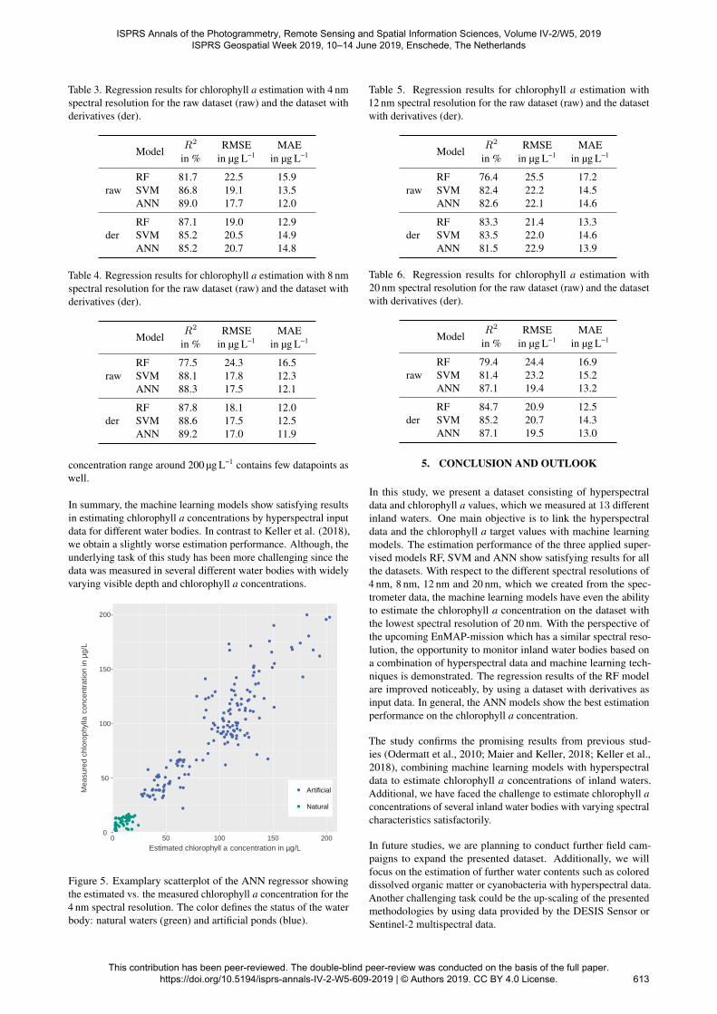
Table 3. Regression results for chlorophyll a estimation with 4 nmspectral resolution for the raw dataset (raw) and the dataset withderivatives (der).

ModelR2 RMSE MAE

in % in µg L−1 in µg L−1

rawRF 81.7 22.5 15.9SVM 86.8 19.1 13.5ANN 89.0 17.7 12.0

derRF 87.1 19.0 12.9SVM 85.2 20.5 14.9ANN 85.2 20.7 14.8

Table 4. Regression results for chlorophyll a estimation with 8 nmspectral resolution for the raw dataset (raw) and the dataset withderivatives (der).

ModelR2 RMSE MAE


rawRF 77.5 24.3 16.5SVM 88.1 17.8 12.3ANN 88.3 17.5 12.1

derRF 87.8 18.1 12.0SVM 88.6 17.5 12.5ANN 89.2 17.0 11.9

concentration range around 200 µg L−1 contains few datapoints aswell.

In summary, the machine learning models show satisfying resultsin estimating chlorophyll a concentrations by hyperspectral inputdata for different water bodies. In contrast to Keller et al. (2018),we obtain a slightly worse estimation performance. Although, theunderlying task of this study has been more challenging since thedata was measured in several different water bodies with widelyvarying visible depth and chlorophyll a concentrations.

●

●

●

●

●

●●

●

●

●

●

●

●

●

●

●

●

●

●●

●

●

● ●

●

●

●

●

●

●

●

●

●

●

●

●

●

●

●

●

●

●

●

●

●

●●

●

●

●

●

●

●

●

●

●

●

●

●

●

●●

●●

●

●

●

●

●

●

●

●

●

●

●

●

●

●

●

●

●

●

●

●

●

●

●

●

●

●

●

●

●

●

●

●

● ●

●

●

●

●

●

●

●

●

●

●

●

●

●

●

●

●

●

●

●

●

●

●

●

●

●

●

●

●

●

●

●

●

●

●

●

●

● ●

●

●

●

●

●

●

●

●

●

●

●

●

●

●

●

●

●

●

●

●

●

●

●

●

●

●●

●

●

●

●

●

●

●

●

●

●

●

●

●

●

●

●

●

●

●

●

●

●

●

●

●

●

●

●

●

●

●

●

●

●

●

●

●

●

●●

●

●

●

●

●

●

●

●

●

0

50

100

150

200

0 50 100 150 200

Estimated chlorophyll a concentration in µg/L

Mea

sure

d ch

loro

phyl

la c

once

ntra

tion

in µ

g/L

●

●

Artificial

Natural

Figure 5. Examplary scatterplot of the ANN regressor showingthe estimated vs. the measured chlorophyll a concentration for the4 nm spectral resolution. The color defines the status of the waterbody: natural waters (green) and artificial ponds (blue).

Table 5. Regression results for chlorophyll a estimation with12 nm spectral resolution for the raw dataset (raw) and the datasetwith derivatives (der).

ModelR2 RMSE MAE


rawRF 76.4 25.5 17.2SVM 82.4 22.2 14.5ANN 82.6 22.1 14.6

derRF 83.3 21.4 13.3SVM 83.5 22.0 14.6ANN 81.5 22.9 13.9

Table 6. Regression results for chlorophyll a estimation with20 nm spectral resolution for the raw dataset (raw) and the datasetwith derivatives (der).

ModelR2 RMSE MAE


rawRF 79.4 24.4 16.9SVM 81.4 23.2 15.2ANN 87.1 19.4 13.2

derRF 84.7 20.9 12.5SVM 85.2 20.7 14.3ANN 87.1 19.5 13.0

5. CONCLUSION AND OUTLOOK

In this study, we present a dataset consisting of hyperspectraldata and chlorophyll a values, which we measured at 13 differentinland waters. One main objective is to link the hyperspectraldata and the chlorophyll a target values with machine learningmodels. The estimation performance of the three applied super-vised models RF, SVM and ANN show satisfying results for allthe datasets. With respect to the different spectral resolutions of4 nm, 8 nm, 12 nm and 20 nm, which we created from the spec-trometer data, the machine learning models have even the abilityto estimate the chlorophyll a concentration on the dataset withthe lowest spectral resolution of 20 nm. With the perspective ofthe upcoming EnMAP-mission which has a similar spectral reso-lution, the opportunity to monitor inland water bodies based ona combination of hyperspectral data and machine learning tech-niques is demonstrated. The regression results of the RF modelare improved noticeably, by using a dataset with derivatives asinput data. In general, the ANN models show the best estimationperformance on the chlorophyll a concentration.

The study confirms the promising results from previous stud-ies (Odermatt et al., 2010; Maier and Keller, 2018; Keller et al.,2018), combining machine learning models with hyperspectraldata to estimate chlorophyll a concentrations of inland waters.Additional, we have faced the challenge to estimate chlorophyll aconcentrations of several inland water bodies with varying spectralcharacteristics satisfactorily.

In future studies, we are planning to conduct further field cam-paigns to expand the presented dataset. Additionally, we willfocus on the estimation of further water contents such as coloreddissolved organic matter or cyanobacteria with hyperspectral data.Another challenging task could be the up-scaling of the presentedmethodologies by using data provided by the DESIS Sensor orSentinel-2 multispectral data.



613

ACKNOWLEDGEMENT

The research is part of the WAQUAVID project funded by theGerman Federal Ministry of Education and Research. We thankour project partners Christian Moldaenke and Andre Zaake forproviding the AlgaeLabAnalyser during the whole field campaign,Philipp Wagner and Eva-Maria Klier for their help regarding themeasurements as well as Stefan Hinz for his support.

References

Breiman, L., 2001. Random Forests. Machine learning 1, pp. 5–32.

Dall’Olmo, G., Gitelson, A. A. and Rundquist, D. C., 2003. Towards aunified approach for remote estimation of chlorophyll-a in both terres-trial vegetation and turbid productive waters. Geophysical ResearchLetters 30(18), pp. 911.

Decker, A. G., Malthus, T. J., Wijnen, M. M. and Seyhan, E., 1992. Theeffect of spectral bandwidth and positioning on the spectral signatureanalysis of inland waters. Remote Sensing of Environment 41(2-3),pp. 211–225.

Gitelson, A., 1992. The peak near 700 nm on radiance spectra of algaeand water: Relationships of its magnitude and position with chloro-phyll concentration. International Journal of Remote Sensing 13(17),pp. 3367–3373.

Gitelson, A. A., Schalles, J. F. and Hladik, C. M., 2007. Remotechlorophyll-a retrieval in turbid, productive estuaries: Chesapeake Baycase study. Remote Sensing of Environment 109(4), pp. 464–472.

Gons, H. J., 1999. Optical Teledetection of Chlorophyll a in Turbid InlandWaters. Environmental Science & Technology 33(7), pp. 1127–1132.

Gonzlez Vilas, L., Spyrakos, E., Palenzuela, T. and M., J., 2011. Neuralnetwork estimation of chlorophyll a from MERIS full resolution datafor the coastal waters of Galician rias (NW Spain). Remote Sensing ofEnvironment 115(2), pp. 524–535.

Hunter, P. D., Tyler, A. N., Presing, M., Kovacs, A. W. and Preston, T.,2008. Spectral discrimination of phytoplankton colour groups: Theeffect of suspended particulate matter and sensor spectral resolution.Remote Sensing of Environment 112(4), pp. 1527–1544.

Keiner, L. E. and Yan, X.-H., 1998. A Neural Network Model for Esti-mating Sea Surface Chlorophyll and Sediments fromThematic MapperImagery. Remote Sensing of Environment 66(2), pp. 153–165.

Keller, S., Maier, P. M., Riese, F. M., Norra, S., Holbach, A., Borsig, N.,Wilhelms, A., Moldaenke, C., Zaake, A. and Hinz, S., 2018. Hyperspec-tral Data and Machine Learning for Estimating CDOM, Chlorophyll a,Diatoms, Green Algae and Turbidity. International journal of environ-mental research and public health.

Kim, Y. H., Im, J., Ha, H. K., Choi, J.-K. and Ha, S., 2014. Machinelearning approaches to coastal water quality monitoring using GOCIsatellite data. GIScience & Remote Sensing 51(2), pp. 158–174.

Maier, P. M. and Keller, S., 2018. Machine learning regression on hy-perspectral data to estimate multiple water parameters. arXiv preprintarXiv.

Maier, P. M., Hinz, S. and Keller, S., 2018. Estimation of Chlorophyll a,Diatoms and Green Algae Based on Hyperspectral Data with MachineLearning Approaches. 38. Wissenschaftlich-Technische Jahrestagungder DGPF und PFGK18 Tagung in Munchen 27, pp. 49–57.

Morel, A. and Prieur, L., 1977. Analysis of variations in ocean color1.Limnology and Oceanography 22(4), pp. 709–722.

Odermatt, D., Giardino, C. and Heege, T., 2010. Chlorophyll retrievalwith MERIS Case-2-Regional in perialpine lakes. Remote Sensing ofEnvironment 114(3), pp. 607–617.

O’Reilly, J. E., Maritorena, S., Mitchell, B. G., Siegel, D. A., Carder,K. L., Garver, S. A., Kahru, M. and McClain, C., 1998. Ocean colorchlorophyll algorithms for SeaWiFS. Journal of Geophysical Research:Oceans 103(C11), pp. 24937–24953.

Palmer, S. C., Kutser, T. and Hunter, P. D., 2015. Remote sensing of inlandwaters: Challenges, progress and future directions. Remote Sensing ofEnvironment 157, pp. 1–8.

Ripley, B. D., 1996. Pattern recognition and neural networks. CambridgeUniversity Press, Cambridge and New York.

Rundquist, D. C., 1996. Remote Measurement of Algal Chlorophyll inSurface Waters: The Case for the First Derivative of Reflectance Near690 nm.

Schalles, J. F., Gitelson, A. A., Yacobi, Y. Z. and Kroenke, A. E., 1998.Estimation of chlorophyll a from time series measurements of high spec-tral resolution reflectance in an eutrophic lake. Journal of Phycology34(2), pp. 383–390.

Vapnik, V. N., 1995. The Nature of Statistical Learning Theory.

Zhou, L., Xu, B., Ma, W., Zhao, B., Li, L. and Huai, H., 2013. Evalua-tion of Hyperspectral Multi-Band Indices to Estimate Chlorophyll-AConcentration Using Field Spectral Measurements and Satellite Data inDianshan Lake, China. Water 5(2), pp. 525–539.



614

estimating chlorophyll a concentrations of several …

Documents