Rachel Sleeter U.S. Geological Survey 345 Middlefield Rd. Menlo Park, CA. 94025 rsleeter@usgs.gov Nathan Wood U. S. Geological Survey Vancouver, WA. nwood@usgs.gov

ESTIMATING DAYTIME AND NIGHTTIME POPULATION DENSITY FOR COASTAL COMMUNITES IN OREGON

Abstract: Hazard preparedness has become a critical issue for local populations who are potentially vulnerable to natural disasters. Essential to preparedness planning is determining where people are likely to be located, which varies from day to night. The fundamental approaches to geographic scale and cartographic representation are an integral aspect of how population distribution is represented over space. Using a dasymetric mapping technique, residential populations are estimated by interpolating the census block values to 10 m pixels based on parcel-level land use and density. To determine daytime population estimates, a quantitative employee database gives x,y point locations of each business and exact numbers of how many people are employed within a coastal community. From census records, we can estimate the number of people who are leaving their residences during the daytime to go to work outside of a tsunami hazard zone.

INTRODUCTION Local communities potentially affected by natural disasters are taking strides to

minimize loss in the event of a catastrophic event. Scientific analysis and technological advances have led to the growth of geographic tools that have the capacity to aid local jurisdictions in emergency planning. The use of Geographic Information Systems (GIS) allows users to visually and statistically characterize populations at risk within hazard zones. The spatial distribution of people across the landscape can be represented in a variety of ways within a GIS mapping framework. The goal of this research is to develop an accurate representation of population distribution along the Oregon Coast, estimating daytime verses nighttime fluctuations in the event of a Cascadia Subduction Zone (CSZ) tsunami. The implementation of a microscale map of population density in the daytime and nighttime provides a realistic snapshot of who is on the ground when the tsunami event occurs, highlighting higher risk areas during response and recovery efforts. By using a dasymetric mapping technique to manipulate U.S. Census enumeration units, population values are distributed to 10-m grid cells with the input of a tax parcel dataset acting as the primary ancillary indicator of inhabited land use/land cover. The importance of

1

symbolizing population density within a semicontinuous surface rather than with discrete areal units represents the continuous nature of the population density ratio (people/sq km).

A dasymetric mapping method usually employs land-use/land-cover data extracted

from remotely sensed images to gain an improved estimation of where people actually reside (Liu 2004). An areal interpolation technique is then applied to disaggregate census population data into homogenous residential or commercial zones reflecting inhabited land use (Mennis 2003). Results using this methodology vary depending on the quality and accuracy of the land-use/land-cover data input. Contrary to using thematic land-use/land-cover data derived from remotely sensed imagery, this research applies tax parcel data with detailed land-use attribute codes as the primary indicator of what parcels are inhabited at night and at what density. The methodology for calculating daytime population density is more complex due to the lack of standardized data collection of people’s whereabouts during a given work day. A combination of employment, schools, age, and daytime residential variables were derived from the U.S. Census and business databases to estimate population distribution per land parcel during the workday.

Dasymetric Mapping

Many methods for population estimation have been practiced in the GIS and Remote Sensing fields. Cartographers prefer dasymetric mapping for population density over other methods because of its ability to more realistically distribute data over geographic space. Similar to choropleth maps, a dasymetric map utilizes standardized data (i.e. census data). However, rather than using arbitrary administrative boundaries to symbolize population distribution, a dasymetric approach introduces ancillary information to redistribute the standardized data into zones of increased homogeneity taking into consideration actual changing densities within the boundaries of the enumeration district (see Figure 1). If appropriately approached, dasymetric mapping is far superior to choropleth mapping in relaying the underlying statistical surface of semicontinuous data (Mennis 2003). This type of mapping has been described as an intelligent alternative to choropleth mapping in an attempt to improve area homogeneity. Thus, new zones are created that directly relate to the function of the map, capturing spatial variations in population density. Land-cover data can indicate residential areas for the delineation of new homogeneous zones. The census populations can be redistributed to the new zones, resulting in a more accurate portrayal of where people live within an administrative boundary. Dasymetric mapping also corrects for the ecological fallacy that may occur within choropleth mapping when the interpretation of statistical data refers to the group as a whole rather than the individuals that comprise it.

2

_________________________________________________________________________

Figure 1. Data may be collected for individual households, as shown on by the four blocks the left. In this example, assume that every male/female pair represents a household of five persons. However, due to confidentiality, data is often aggregated into larger units of analysis, as shown by the four blocks on the right. Examples of levels of aggregation used in this situation are census blocks, zip codes, area codes, city limits, and county boundaries. Dasymetric mapping attempts to disaggregate the four figures on the right into their original state on the left. STUDY AREA

Cascadia Subduction Zone Tsunamis pose significant threats to coastal communities in the U.S. Pacific

Northwest due to the numerous potential seismic sources around the Pacific Ocean margin. The most recent example of a tsunami associated with the magnitude 9.2 earthquake originating in Alaska caused property damage and life loss along the western seaboard of the United States occurred on March 27, 1964. Historical and geological evidence suggest the Pacific Northwest has experienced numerous tsunamis in the past and is likely to experience more in the future (Satake et al. 1996; Atwater & Hemphill-Haley 1997; Peters et al. 2001; Priest et al. 2001). Tsunamis related to earthquakes emanating from the CSZ (see Figure 2) are potentially the most threatening as modeling efforts suggest a CSZ earthquake could generate a series of seismic sea waves possibly 8-m or higher that inundate the Oregon coast approximately 30 minutes after initial ground shaking (Myers et al. 1999). Such a scenario and its potential impacts are analogous to the recent catastrophic tsunamis in the Indian Ocean. Recurrence intervals of past CSZ seismic activity ranges from 300 to 600 years (Atwater and Hemphill-Haley 1997), with the last earthquake occurring in 1700 A.D. (Satake et al. 1996). This suggests the Pacific Northwest is now within the window for another CSZ earthquake and tsunami.

3

Figure 2. The Cascadia Subduction Zone stretches from mid-Vancouver Island to Northern California. It separates the Juan de Fuca Plate from the North American Plate. The oceanic crust of the Pacific Ocean is pushed toward and beneath the continent at a rate of 40 mm/yr. The large fault zone has the potential to produce a magnitude 9.0 earthquake causing destruction along the Pacific Coast.

A critical first step in managing these threats is to understand who is exposed to these hazards. In the United States, emergency managers have access to decadal census data that summarizes residential populations. However, in many coastal communities, there are typically greater numbers of nonresidents (e.g. employees, tourists) in high tsunami hazard zones (Wood and Good 2004). Emergency managers need to estimate the number of residents, employees, and visitors who could potentially be exposed to possible hazards if they are to develop realistic risk reduction and preparedness strategies. One way to do this is to use ambient population data, which attempts to quantify the actual distribution of individuals in an area. Datasets like LandScan, developed as part of the Oak Ridge National Laboratory (ORNL) Global Population Project (ORNL 2005), focus on ambient population and have been used for post-disaster assessments at the global scale. Ambient population is defined as the number of people likely to be in an area as opposed to residents alone, with population counts for each 1-km2 cell being based on probability coefficients. Verified to be accurate to within 10% of the given values, these coefficients are based on road proximity, slope, land cover, and nighttime lights. However, with a 1-km2 cell size, this dataset is believed to be too coarse for local planning. The research we present here focuses on the development of a method to model daytime and nighttime population at the local level. The case study looks at Clatsop County, Oregon; however, the input data and methodology have been developed to apply to other local communities involved with hazard planning and response.

4

METHODS

Areal Interpolation To model residential population distribution to actual occupied areas, areal

interpolation is often employed. Areal interpolation is the process of estimating the values of one or more variables in a set of target polygons based on known values that exist in a set of source polygons (Hawley et al. 2005). The overlay method is one that does not use ancillary data as a calibrator to redistribute values, instead it uses areal weighting, which interpolates based on the proportional area derived from the intersection between the source and target polygons (Lam 1980; Flowerdew and Green 1993). In more recent methods (Holloway et al. 1997; Liu 2004; Mennis 2003), ancillary data is used as an aid to give a more precise indication of what exists on the statistical surface. The easiest dasymetric mapping approach with remote-sensing derived land-use data is the binary division approach in which land use is classified to “populated” or “unpopulated” and census populations are simply redistributed to populated areas (Holt et al. 2004; Fisher and Langford 1996, and Langford and Unwin 1994). Holloway et al. (1997) combines multiple ancillary datasets to detect and remove uninhabited lands from the area of analysis. Four types of land use/land cover were ruled out, including census blocks with zero population, all lands owned by local, State, or Federal government, all corporate timberlands, and all water or wetlands, as well as all open and wooded areas with terrain slopes more than 15% (Holloway et al. 1997). To redistribute the census population to the ancillary feature classes, a predetermined percentage was assigned to each class. The subjectivity and accuracy of this percentage assignment (e.g., 80% of the population to urban polygons, 10% to open polygons, and 5% to agriculture and wooded polygons) can be argued because of the absence of empirical evidence. Mennis (2003) used a combination of areal weighting and a three-tier, urban-classification method derived from thematic satellite data to break down census tracts into homogenous residential zones. To account for the relative densities in each urban class, empirical sampling provides a proportional density fraction used as a constant value in the interpolation. The equations used in the interpolation (see Appendix I) have been converted into an ArcObjects script and applied to the methodology used for the nighttime distribution for the Oregon Coast.

The quality of the interpolation estimates depends largely on (1) how source zones

and target zones are defined, (2) the degree of generalization in interpolation process, and (3) the characteristics of the partitioned surface (Lam 1983). We use the census-block group as the source polygons of known values and a tax-parcel database as the target polygons. The parcels have many attributes that allow for a hierarchical density weighting relative to building type, use, and description. For example, an apartment complex indicates very high density, a single family home indicates a medium density, and a large acreage estate indicates low density. The parcel database is divided into four density classes, high, medium, low, and exclusion, to act as a hierarchical measure within the interpolation process. There are two main incentives for utilizing parcel data for this particular dasymetric mapping approach. First, to create a methodology that can be transferred to other hazard prone regions, the data inputs necessary have to be accessible, affordable, and uniformly structured. Parcel data exists for every county in the United States, whether it is in digital or analog format, the data is available and can be converted for use by local communities. Second, the scale, resolution, and accuracy derived from

5

parcel data are significantly better than most remote-sensing derived land-use/ land-cover products (e.g. National Land Cover Dataset – 30-m grid resolution). The smallest parcel in area equaled about 100 sq. ft. which allows the minimum mapping unit to be a 10-m grid resolution. To capture land-cover classifications at such a high resolution, the more common approach would be to use remotely sensed imagery with high spatial resolution (e.g. IKONOS – 4-m color). However, due to the spatial and spectral heterogeneity of the urban environment, inconsistencies become prevalent when trying to characterize built-up structures mixed in with vegetation cover (Harold et al. 2002). Consequently, parcel data becomes a more practical option for delineating residential neighborhoods into density classes.

Nighttime Population Estimation To determine nighttime population for Clatsop County, Oregon, a combination of

prior methods are used (Mennis 2003; Holloway et al. 1997) that led to the development of three urban-residential classes and one exclusion class, which represents all uninhabited areas (see Figure 3). The parcel attributes describe the land-use and building types present on each parcel of land and are then reclassified into four classes: high density, medium density, low density, and uninhabited. The newly created land-use/land-cover layer is converted to raster format at a 10-m resolution acting as the target zones in the interpolation of census-block groups. We use an ArcObjects, Visual Basic script to automate the areal interpolation using the principles of areal weighting and empirical sampling of relative densities which result in a three-tier distribution of population density at a 10-m pixel resolution.

Daytime Population Estimation The shift in population during business hours is more difficult to capture at a high-

resolution due to the lack of standardized daytime population data. The census offers a daytime population estimate at the census-tract level based on a simple equation taking into account total in-commuters and total out-commuters. This is a reliable source for regional assessments; however, the tract unit is arguably too large for emergency response at the community level and does not address the spatial issues associated with data aggregation. We use the InfoUSA database, parcel data, school student counts, and census block-group employment and age data to identify inhabited daytime land-use. The InfoUSA database gives the x,y location of every business in the study area and includes many attributes, most importantly the number of employees at each location. Parcel data provides detailed descriptions of industrial, commercial, and mixed land use that can be spatially joined to the x,y location of each business. Clatsop County offers information on the internet about how many students attend each school. Finally, the 2000 Census SF3 provides a total number of workers over age 16 per block group, and specifies if the worker leaves the home or works at home. For this study it is not important to understand the destinations of workers working away from home; we are only concerned with whether or not the worker is leaving the home. Once the worker is determined away from home, the worker gets subtracted completely. This can be done with confidence due to the fact that we have an employee database with exact point locations, so the worker that has been subtracted will be gained in the correct spatial location later in the calculation. The transfer of population to the daytime inhabited areas is done with a simple equation (see Table 1).

6

_________________________________________________________________________

A B

Figureinhabit(C) replow (ye

run thpopularesidesourceschoochildrlow prcommInfoUof wointerplayer iidentifonline(http:/been rpopula

C

3. (A) represents total number of peed (red) vs. uninhabited (green) withresents an urban 3-class method, whllow) population class based on land

With the adjusted daytime porough the same automated Arction estimates. Three iteratio

ntial parcels using the existing population value for this itera

l and who are assumed to be reen not attending school, and stoportion of the daytime populercial and industrial parcels fuSA to demarcate employmentrk from home values taken froolation is performed; howevers a binary classification code ies schools using the parcel d information about each schoo/oregon.schooltree.org/Clatsopun separately, the three raster tion dataset at a 10-m resolut

ople, aggregated by census delineated unit (B) represents populations evenly distributed within the inhabited land use and ere populations are distributed in high (red), medium (pink), and -use class code and areal weighting.

pulation per block group, an areal interpolation can be Objects script that we used for the nighttime ns are run through the script; the first distributing to stratified density classifications (see Table 1). The tion represents all persons who are not employed or in siding at home. The elderly, unemployed, small ay-at-home parents are some examples of this a very ation. The second iteration uses land use identified by sed together with business locations derived from

areas. The source population value is a combination m the census and the InfoUSA database. An areal , different from the nighttime estimates the land-use of inhabited versus uninhabited. The third iteration atabase and extracts the number of students from l district in Clatsop Co. -County-Schools.html). When all three iterations have

files are combined to make one master daytime ion.

7

Equation Used to Determine Daytime Population Per Block-Group

Census SF3 - BG Level

Total Population (A)

Total workers - Age 16+ (B)

Work Outside of Residence (C)

Work From Home (D)

Age 5-18 (In School- Not at home) (E)

Total People Leaving their Home (F) = (C + E)

250 100 90 10 85 175

InfoUSA Database

Clatsop Co., OR. Education Website

Total population remaining in their residence (G) = (A) - (F)

# of Employees (InfoUSA) (H)

# of Employees per block group (I) = (H) + (D)

# of students per school (Aggregated to block-group) (J)

TOTAL DAYTIME POP PER BLOCK GROUP (K) = (G) + (I) + (J)

75 53 63 70 208 Table 1. Combination of census employment data and age data have been combined with InfoUSA and Education data for Clatsop County Oregon to estimate daytime population per block group. This estimate is then distributed via areal interpolation to parcels that are industrial, commercial, or mixed-use.

DISCUSSION AND RESULTS

The population distribution model for daytime and nighttime distribution has been completed for Clatsop Co., Oregon, as a case study for future application to the entire Oregon Coast. However, within the mechanics and methodology of this research, we found some errors associated with the data inputs. As with any model study, the quality of the output is no better than the quality of the input. In this case, the InfoUSA business database, provides x,y locations in a point feature class. The location of the point corresponds to the address that appears to be either at the centerline of the street or close to where the mailbox would be situated. The business data contains the most important aspect of daytime population distribution, which is the number of employees at each location, so the spatial registration and placement of the points presents a problem when trying to fuse the parcel land-use codes with the business data. To compare the daytime population to the nighttime population, the relative spatial size of the parcels needs to be preserved in the distribution rather than distributing the numbers of employees to a single point, leading to the decision to spatially join each business point to the parcel in closest proximity.

To analyze the difference between the daytime and the nighttime population distributions, the 10-m grids for each time of day are subtracted from one another generating a positive to negative range revealing the areas that have changed most significantly. Because there are only five coastal cities in Clatsop County, we analyzed

8

five 0.5-km2 sample blocks containing the highest change. Figure 4 shows how the U.S. Geological Survey’s digital orthophoto quadrangles (DOQs) were used as a reference for land-use/land-cover interpretation with the daytime high-level changes overlaid. One of the major discrepancies between the businesses versus parcel data that became apparent when referencing the DOQs was the number of parcels that appeared to be in the commercial industrial zones, but had zero population. By referencing the DOQs and the parcel database, we estimated that 24% of overall parcels should have been eligible for daytime population distribution due to the commercial/industrial land-use type in the parcel database. DOQs are black and white and have a resolution of 1-m, but prove to be a good reference for verifying overall land-cover type. The spectral signature cannot be measured because the imagery has only one band, but building density and brightness can be detected, indicating commercial and industrial areas.

Figure 4. Sample blocks of 0.5-km2 are placed in the highest areas of daytime population fluctuation. DOQs are used as a land-cover reference revealing the errors stemming from the data fusion between the business data and the parcel data. Twenty-four % of parcels in these sample blocks are vacant and should have a proportion of the population.

Most parcels are representative of inhabited land uses correlating to their relative area; however, some of the parcels in the lowest density zones are very large in area with only one structure. The dasymetric method is still subject to the problem of an even distribution assumption within subzones. In other words, although the differences among subzones are recognized, differences within subzones are ignored (Wu et al. 2005). Statistically the population values are very low in these areas, but visually the results are misleading because within large estates or farms the parcel acreage is very large and it appears that the entire area is populated. In the future, this problem can be remedied with additional geospatial layers, such as roads or structures.

The two most populated cities in Clatsop County are Astoria (9,813 residents) and

Seaside (5,900 residents). In Astoria the net daytime population decreases (almost by half)

9

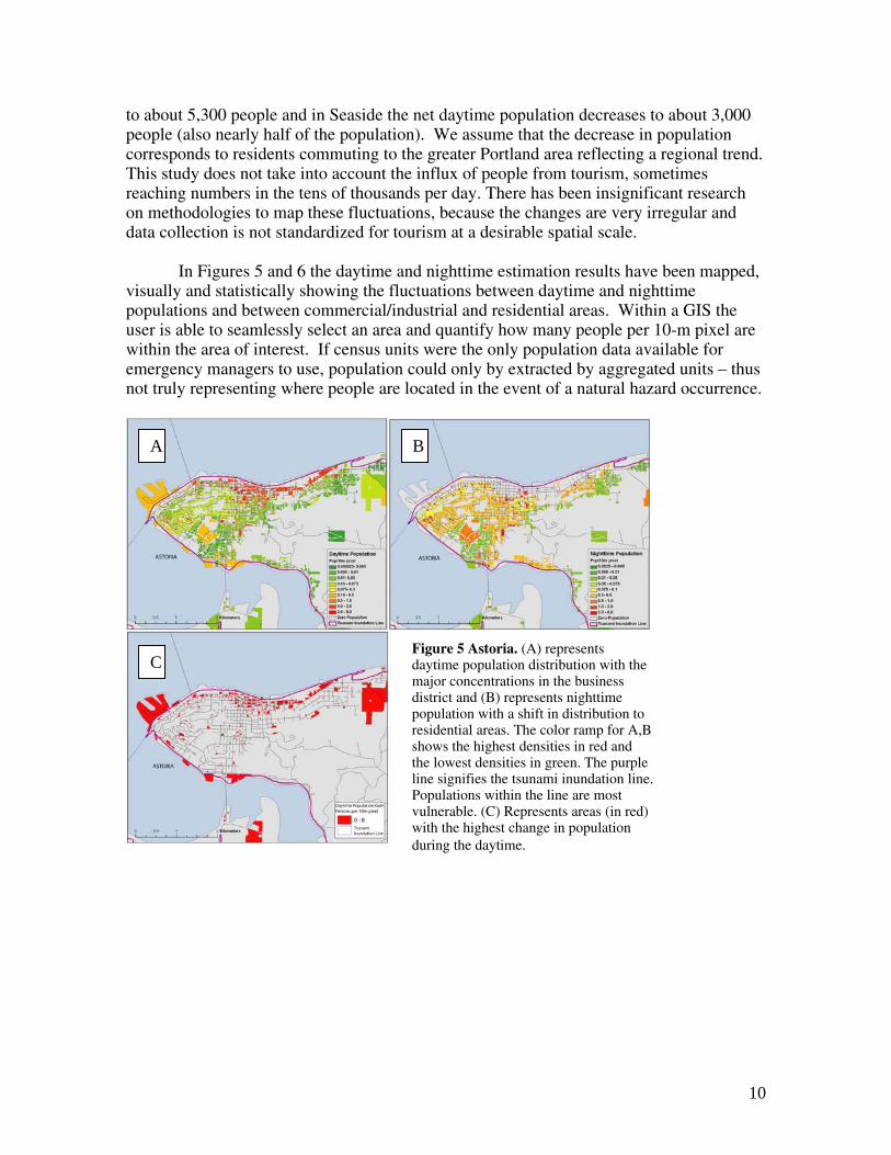
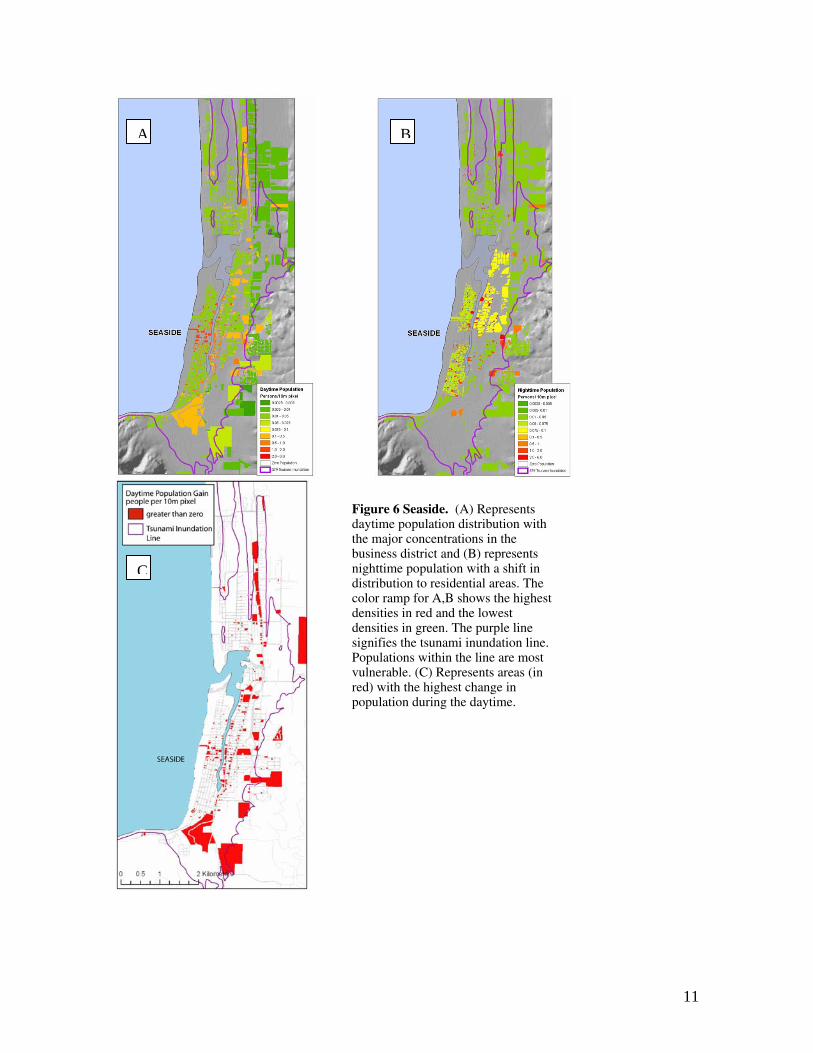
to about 5,300 people and in Seaside the net daytime population decreases to about 3,000 people (also nearly half of the population). We assume that the decrease in population corresponds to residents commuting to the greater Portland area reflecting a regional trend. This study does not take into account the influx of people from tourism, sometimes reaching numbers in the tens of thousands per day. There has been insignificant research on methodologies to map these fluctuations, because the changes are very irregular and data collection is not standardized for tourism at a desirable spatial scale.

In Figures 5 and 6 the daytime and nighttime estimation results have been mapped,

visually and statistically showing the fluctuations between daytime and nighttime populations and between commercial/industrial and residential areas. Within a GIS the user is able to seamlessly select an area and quantify how many people per 10-m pixel are within the area of interest. If census units were the only population data available for emergency managers to use, population could only by extracted by aggregated units – thus not truly representing where people are located in the event of a natural hazard occurrence.

A B

Figure 5 Astoria. (A) represents daytime population distribution with the major concentrations in the business district and (B) represents nighttime population with a shift in distribution to residential areas. The color ramp for A,B shows the highest densities in red and the lowest densities in green. The purple line signifies the tsunami inundation line. Populations within the line are most vulnerable. (C) Represents areas (in red) with the highest change in population during the daytime.

C

10

A B

Figure 6 Seaside. (A) Represents daytime population distribution with the major concentrations in the business district and (B) represents nighttime population with a shift in distribution to residential areas. The color ramp for A,B shows the highest densities in red and the lowest densities in green. The purple line signifies the tsunami inundation line. Populations within the line are most vulnerable. (C) Represents areas (in red) with the highest change in population during the daytime.

C

11

CONCLUSION

U.S. Census data is based on the residence location, rather than where people work or travel during the day. Additionally, the census aggregates this information into larger enumeration units that obscure the underlying statistical surface. This research explores a dasymetric method to map daytime and nighttime population at the parcel level for the application and use at the local level for emergency response. In the event of a CSZ generated tsunami off the coast of the Pacific Northwest, a detailed, high-resolution representation of population density is desirable in order to visually and statistically identify the areas most vulnerable. Through extensive literature review, we explore an areal interpolation method for estimating nighttime population density at a 10-m pixel resolution. The method used for estimating daytime population was very experimental because little research has attempted to model daytime population.

This research uses data that is accessible and affordable at the county level, while

maintaining quality and high accuracy in the end result. The parcel database, available nationwide proves to be a good alternative to remotely sensed imagery for classifying land-use codes for daytime and nighttime population estimates. We also incorporated data from InfoUSA to locate every business with the exact number of employees. This dataset was a very valuable addition for estimating daytime population; however, due to registration errors, some of the parcel land-use codes did not match with the business x,y locations. This error caused 24% of the daytime parcels to be falsely classified. The addition of a structures layer and a roads layer would improve the land-use delineations in low-density areas because the parcel size in these areas does not represent the small population on the ground.

By making these improvements to the input data, our goal for future research is to

build a geospatial tool or extension that will streamline the areal interpolation process. We continue to research the input data and its overall accuracy for the dasymetric mapping technique, with the intention to help local communities prone to natural disasters. By generating a downloadable tool with affordable data layers as inputs, this method will be an attractive alternative to the standard aggregated census data that limit geospatial research for emergency management and response.

12

APPENDIX I – Mennis (2003)

a) duc = Puc/(Pbc + Plc + Pnc) (1) where duc = population-density fraction of urbanization class u in county c, Puc = population density (persons/900 m2) of urbanization class u in county c, Pbc = population density (persons/900 m2) of urbanization class h (high) in county c, Plc = population density (persons/900 m2) of urbanization class l (low) in county c, and Pnc = population density (persons/900 m2) of urbanization class n (nonurban) in county c.

b) baub = (nub/nb)/0.33 (2)

where aub = area ratio of urbanization class u in block-group b, nub = number of grid cells of urbanization class u in block-group b, and nb = number of grid cells in block-group b.

c) fubc = (duc*aub)/ [(dhc*ahb) + (dlc*alb) + (dnc*anb)] (3)

where fubc = total fraction of urbanization class u in block-group b and in county c, duc = population-density fraction of urbanization class u in county c, aub = area ratio of urbanization class u in block-group b, dhc = population-density fraction of urbanization class h (high) in county c, dlc = population-density fraction of urbanization class l (low) in county c, dnc = population-density fraction of urbanization class n (nonurban) in county c, ahb = area ratio of urbanization class h (high) in block-group b, alb = area ratio of urbanization class l (low) in block-group b, and anb = area ratio of urbanization class n (nonurban) in block-group b.

d) popubc = (fubc*popb)/nub (4) where popubc = population assigned to one grid cell of urbanization class u in block-group b and in county c, fubc = total fraction for urbanization class u in block-group b and in county c, popb = population of block-group b, and nub = number of grid cells of urbanization class u in block-group b.

13

REFERENCES Atwater, B.F., and Hemphill-Haley, E. 1997. Recurrence intervals for great earthquakes of the past 3,500 years at northeastern Willapa Bay, Washington, U.S. Geological Survey Professional Paper, 1576, Reston, Virginia. Eicher, C.L., and C.A Brewer. 2001. Dasymetric mapping and areal interpolation: implementation and evaluation. Cartography and Geographic Information Science 28(2): 125-138. Fisher, P.F. and M. Langford. 1996 Modeling sensitivity to accuracy in classified imagery: A study of areal interpolation and dasymetric mapping. Professional Geographer. 48(3): 299-309. Flowerdew, Robin and Mick Green. 1994. Areal interpolation and types of data. Spatial Analysis and GIS edited by Stewart Fotheringham and Peter Rogerson. London, Bristol: Taylor & Francis Ltd. Hawley, K. and Harold Moellering. 2005. A comparative analysis of areal interpolation methods. Cartography and Geographic Information Science. (32)4:411-423. Herold, M., et al. 2002. Object-oriented mapping and analysis of urban land use/land cover using IKONOS data. Proceedings of the 22nd EARSEL symposium, Prague, June 2002. Holloway, S., J. Schumacher, and R. Redmond. 1997. People & Place: Dasymetric mapping using Arc/Info. Cartographic Design Using ArcView and Arc/Info, Missoula: University of Montana, Wildlife Spatial Analysis Lab. Holt, J.B., Lo, C.P., and T.W. Hodler. 2004. Dasymetric estimation of population density areal interpolation of census data. Cartography and Geographic Information Science. 31(2):101-121. infoUSA, 2005, Employer Database, unpublished data, acquired on 7/07/2005, <http://www.infousagov.com/index.asp> Klein, R., R. Nicholls, and F. Thomalla. 2003. Resilience to natural hazards: How useful is this concept? Environmental Hazards 5:35-45 Lam, Nina Siu-Ngan. 1983. Spatial interpolation methods: A review. The American Cartographer, 10(2): 129-149. Langford, M. and D.J. Unwin. 1994. Generating and mapping population-density surfaces within a geographical information-system. Cartographic Journal. 31(1):21-26. Liu, X. 2004. Dasymetric mapping with image texture. ASPRS annual conference proceedings, Denver, Colorado, May 2004.

14

McPherson, T. et al. 2006. A day –night population exchange model for better exposure and consequence management assessments. The 86th AMS Annual Meeting, Atlanta, GA. February 1, 2006. Mennis, J. 2003. Generating surface models of population using dasymetric mapping. The Professional Geographer, 55(1): 31-42. Myers, E.P., A.M. Baptista, and G.R. Priest (1999): Finite element modeling of potential Cascadia subduction zone tsunamis. Sci. Tsunami Haz., 17 (1), 3–18. Oak Ridge National Laboratory (ORNL) 2005, LandScan Global Population Database, Oak Ridge, TN: Available at http://www.ornl.gov/gist/. Peters, R., Jaffe, B., Peterson C., Gelfenbaum, G., and Kelsey H. 2001. An overview of tsunami deposits along the Cascadia margin. ITS 2001 Proceedings, Session 3, Number 3-3: 479 – 490. Priest, G., and A. Baptista. 1995. Tsunami inundation boundary for the Oregon coast, Open-file reports O-95-28 (Newport North), O-95-29 (Newport South), and O-95-30 (Toledo South), State of Oregon, Department of Geology and Mineral Industries, Portland, Oregon. Priest, G., et al. 1997. Cascadia Subduction Zone tsunamis: hazard mapping at Yaquina Bay, Oregon, Open-file report O-97-34, State of Oregon, Department of Geology and Mineral Industries, Portland, Oregon. Priest, G., Baptista A., Myers III, E., Kamphaus, R. 2001. Tsunami hazard assessment in Oregon. ITS 2001 Proceedings, NTHMP Review Session, Paper R-3: 55- 65. Satake, K., Shimazaki, K., Tsuji, Y., and Ueda, K. 1996. Time and size of a giant earthquake in Cascadia inferred from Japanese tsunami records of January 1700. Nature, 379: 246-249. Wood, N., and Good, J., 2004. Vulnerability of a port and harbor community to earthquake and tsunami hazards: the use of GIS in community hazard planning: Coastal Management, v. 32, no. 3, p. 243-269. Wright, J.K., 1936. A method of mapping densities of population with Cape Cod as an example. Geographical Review 26. Wu, S., Qiu, X., and Wang, L. 2005. Population estimation methods in GIS and Remote Sensing : A review. GIScience & Remote Sensing, 42(1): 80-96.

15