Syracuse University Syracuse University

SURFACE SURFACE

Economics - Faculty Scholarship Maxwell School of Citizenship and Public Affairs

11-2006

Estimating Heterogeneous Capacity and Capacity Utilization in a Estimating Heterogeneous Capacity and Capacity Utilization in a

Multi-Species Fishery Multi-Species Fishery

Ronald G. Feltoven US Marine Fisheries Service

William C. Horrace Syracuse University

Kurt E. Schnier Georgia State University

Follow this and additional works at: https://surface.syr.edu/ecn

Part of the Economics Commons

Recommended Citation Recommended Citation Feltoven, Ronald G.; Horrace, William C.; and Schnier, Kurt E., "Estimating Heterogeneous Capacity and Capacity Utilization in a Multi-Species Fishery" (2006). Economics - Faculty Scholarship. 25. https://surface.syr.edu/ecn/25

This Article is brought to you for free and open access by the Maxwell School of Citizenship and Public Affairs at SURFACE. It has been accepted for inclusion in Economics - Faculty Scholarship by an authorized administrator of SURFACE. For more information, please contact surface@syr.edu.

This is an author-produced, peer-reviewed version of this article. The published version of this document can be found online in the Journal of Productivity Analysis (doi: 10.1007/s11123-009-0139-5) published by SpringerLink.

R. G. Felthoven Alaska Fisheries Science Center, US Marine Fisheries Service, 7600 Sand Point Way NE, Seattle, WA 98115, USA e-mail: ron.felthoven@noaa.gov W. C. Horrace Center for Policy Research, Department of Economics, Syracuse University, 426 Eggers Hall, Syracuse, NY 13244, USA e-mail: whorrace@maxwell.syr.edu K. E. Schnier Department of Economics, Andrew Young School of Policy Studies, Georgia State University, 14 Marietta Street NW, Suite 436, Atlanta, GA 30303, USA e-mail: kschnier@gsu.edu

Estimating heterogeneous capacity and capacity utilization in a multi-species fishery

Ronald G. Felthoven, US Marine Fisheries Service William C. Horrace, Syracuse University Kurt E. Schnier, Georgia State University

Keywords: Stochastic frontier, Efficiency probability JEL Classification C16 D24 Q22

Abstract We use a stochastic production frontier model to investigate the presence of heterogeneous production and its impact on fleet capacity and capacity utilization in a multi-species fishery. We propose a new fleet capacity estimate that incorporates complete information on the stochastic differences between vessel-specific technical efficiency distributions. Results indicate that ignoring heterogeneity in production technologies within a multispecies fishery as well as the complete distribution of a vessel’s technical efficiency score, may lead to erroneous fleet-wide production profiles and estimates of capacity. Our new estimate of capacity enables out-of-sample production predictions which may be useful to policy makers.

1 Introduction Efficient management of natural resources hinges on our ability to monitor resource stocks and the behaviors of the agents using them. The sustainability and viability (both in physical and economic terms) of our resource management plans can, in part, be assessed by estimating the extractive or productive capacity of these agents. Limitations of and uncertainty associated with available data, especially in the fishing industry, make estimating capacity and capacity utilization of these agents particularly difficult. Compounding these difficulties is the heterogeneous nature of agents using the resource. Heterogeneity implies that multiple production technologies may exist, which must be accounted for when measuring capacity and capacity utilization. Otherwise, capacity estimates may be erroneous and lead to inappropriate policy recommendations.

Given growing concern over excess capacity in many natural resource environments (FAO 1998) and the need to assess capacity to prioritize the settings in which direct problems exist, it is important to develop methods that investigate and control for production heterogeneity. Furthermore, it is important that we use measures that better incorporate information on the statistical reliability of our measures of fleet capacity. This research addresses these concerns by estimating heterogeneous capacity and capacity utilization in a multi-species fishery and by proposing a new measure of fleet capacity, which uses information on the stochastic dominance of a vessel’s technical inefficiency distribution (Horrace 2005). Although the biases associated with ignoring latent heterogeneity have been well-documented in the literature, the use of complete distributional information in capacity estimation has never, to the best of our knowledge, been investigated. Our results underscore the complexities that arise in the presence of heterogeneous production technologies (a common situation in multi-species, multi-gear fisheries) as well as the benefits of using higher moment information on technical inefficiency in capacity estimation.

Capacity estimates are desirable because overcapacity is often cited as a major reason for overexploitation of fisheries around the globe (FAO 1998). Common symptoms of excess capacity are dwindling fish stocks, an accelerated ‘‘race for fish’’ resulting in a shorter fishing season, and excessive investment or input use (‘‘capital stuffing’’) to improve vessel’s odds of catching a larger share of the total catch. Prevalence of these problems has created a need for better estimates of capacity and capacity utilization and improved management instruments that lower the rate of capacity expansion and mitigate the effect of overcapacity in fisheries.

Input controls are often used to combat overcapacity in a fishery, because they homogenize fishing effort and reduce the fleet’s ability to fully use available technology and vessel capital. However, the success of input control regulation is contingent on the vessel’s inability to substitute out of the regulated input into another unregulated input (Kompas et al. 2004). Also, vessel buybacks may be conducted to decrease fleet size and increase the rents of the remaining fishermen, thereby reducing the fleet’s effective capacity and increasing utilization of the remaining vessels (Guyader et al. 2004). Alternatively, it has been argued that a transition to dedicated access privileges, such as individual transferable fishing quotas, is a cost-effective solution to overcapacity as less efficient vessels are bought out by efficient vessels in the fleet (Kompas and Che 2005; Weninger and Waters 2003). Following this transition, a property rights structure reduces the incentives to ‘‘race for fish’’ and yields investments in capacity only when they are economically advantageous. This said, even with all the efforts to control excess

2

capacity and recognition of the associated problems, there does not exist a consensus on the definition of capacity or a means of estimating it (Kompas and Che 2005), so alternative and improved definitions may be warranted.

A common thread among existing studies of fishery capacity is the need to estimate production technology in a manner consistent with economic theory.11 Currently, there are two methods used to estimate fishery production technologies: data envelope analysis (DEA) (Fare et al. 1989; Kirkley et al. 2001; Kirkley et al. 2003; Reid et al. 2003) and stochastic production frontier (SPF) models (Alvarez and Schmidt 2006; Garcia de Hoyo et al. 2005; Felthoven 2002; Kompas and Che 2005; Sharma and Leung 1998; Viswanathan et al. 2003). DEA does not assume a parametric form for the production technology and is therefore a more general and flexible model than its parametric counterpart, the stochastic production frontier (SPF) model. However, SPF models account for production uncertainty while DEA models generally do not. DEA models assume that an agent’s inability to produce the maximal output, given their input mix, is due to agent-specific technical inefficiency. SPF models add a random error component to the production frontier (Aigner et al. 1977; Meeusen and van den Broeck 1977).2 This research adopts a latent stochastic production frontier (LSPF) model (Flores-Lagunes et al. 2007), which synthesizes latent class regressions with SPF models and allows for heterogeneous production frontiers within the fishery.

We base our measure of capacity on the technological-economic approach (Felthoven and Morrison Paul 2004). This measure defines capacity as the maximal feasible output that can be produced given the current level of technological, environmental and economic conditions. This approach provides a primal measure of capacity, because it is based on the physical relationship between inputs and outputs, rather than a dual approach which incorporates behavioral assumptions such as cost minimization or profit maximization. The latter approach is often infeasible given the lack of cost data for most fisheries. Therefore, our definition of capacity is consistent with that conventionally used within the fisheries production literature.

In fisheries, the complexities of capacity estimation may be exacerbated by their multi-species nature. This concern is readily addressed using ray production functions (Felthoven 2002) or distance functions (Orea et al. 2005). Our example is the flatfish fishery of the Bering Sea and Aleutian Islands (BSAI), and we use a distance function to account for its multi-species nature, to control for unobservable variation in the production frontier and to generate our new measure of fleet capacity. Our modeling approach may be used within a ray production function framework, as well. The new capacity measure incorporates information on the complete distribution of a vessel’s technical efficiency to determine the probability of stochastic dominance of its efficiency over other vessels within the fleet. We effectively incorporate probabilities of being efficient into our capacity analysis.

Another motivation for our work is that current estimates of capacity and capacity utilization assume all agents operate with the same production technology. This presumes that each vessel possesses identical output elasticities, elasticities of substitution, marginal rates of transformation, and returns to scale (a single technology). This implies that vessels have the same ability to react and adapt their fishing strategies to regulatory measures enacted to mitigate risks associated with excess capacity.3 However, substantial variation in catch (for a given level of input use) often exists within the fleet. These productive differences may be explained either by differences in technical efficiencies or by asymmetries in the production technologies of different groups of vessels. The latent class model used in this paper allows for both of these phenomena, compared to a single technology assumption which only allows for efficiency differences. Latent heterogeneity in fisheries may be driven by a multitude of factors. Those most commonly cited, yet immeasurable, factors are skipper skill and the ‘‘highliner’’ hypothesis (Kirkley et al. 1998; Pascoe and Coglan 2002; Squires and Kirkley 1999), embodied and disembodied technical change (Kirkley et al. 2004), the processing activity onboard the vessel which often drives fishing rates and targets, and the vintage of technology, to name a few.4

Heterogeneity in behavior has received a fair amount of attention in the stated preference literature through the use of random coefficient models (Train 1998, 2003). In fisheries, random coefficient models have also been used to investigate heterogeneity in site choice modeling for commercial fisheries (Mistiaen and Strand 2000; Smith 2005) as well as recreational fisheries (Provencher and Bishop 2004). Although these models could be adapted to investigate heterogeneity of production technologies within fisheries, they do not allow for the estimation of

1 Ad hoc approaches such as the ‘‘peak to peak’’ method have been used in the past, which prompted many authors to discuss their limitations and suggest more rigorous methodologies. 2 This is an oversimplification of the current state of the literature, but our purpose is not to discuss the relative merits of DEA and SPF models. 3 This is true if we assume that fishermen do not alter their technological choice or targeting strategies for output, measured as the assemblage of species caught within the fishery. Changes in regulatory measures will have many implications on people’s choice sets for inputs and outputs, which will not only reflect technological production possibilities, but also other factors not captured by the production function. 4 A vessel’s age is recorded but vessels are often refurbished and using their build dates to indicate the vintage of their technology is often times erroneous.

3

vesselspecific capacity and capacity utilization measures, which are necessary to inform policy in many contexts.5 To obtain vessel-specific measures of capacity we use the latent class regression method developed by El-Gamal and Grether (1995, 2000): the EC algorithm. Alternatively, one could estimate the latent class production functions using finite mixture regressions (Orea and Kumbhakar 2004). However, finite mixture models estimate the probability of participation in each of the respective classes, whereas the EC algorithm restricts class participation probabilities to be either zero or one. This latter feature allows us to precisely identify class participation and therefore vessel-specific measures of capacity.

2 Defining and estimating heterogeneous capacity We define J different production technology groups (segments), indexed by Within each segment operate vessels, indexed by Each vessel operates in weekly time periods Therefore, a vessel’s deterministic production function is:

Let be a vector of quasi-fixed inputs of production, such as a vessel’s horsepower and size, which are assumed to be fixed during the time horizon analyzed. Let be a vector of exogenous input stocks, such as the current stock level of the target species within a fishery. Let be a vector of variable inputs and potentially the amount of time the fishing gear is deployed. Let be the number of ‘days fished per week’, also a variable input. We make ‘days fished per week’ explicit in our function, because this is the time-varying input that we adjust to calculate capacity for each vessel (any time-varying input or inputs would suffice). Let be a vector of variables to control for differences in technology when multiple methods of production exist and to control for time, space, and environmental factors, such as El Nin˜o and La Nin˜a events. Let be a vector of other species harvested in conjunction with the target species in a multi-species fishery. Finally, let be a scalar measure of a vessel’s level of technical efficiency normalized on the unit interval.6

There are two measures of capacity we are interested in calculating: fleet capacity and a vessel-specific measure of capacity utilization. Furthermore, we refine these estimates by extending them to incorporate two additional dimensions: (1) heterogeneous production technology, and (2) distributional information on technical efficiency rankings. These capacity measures are a function of the available inputs (both quasi-fixed and variable) and maximal output produced from these inputs. These measures may be viewed as a lower bound on fleet capacity because they do not account for the potential reallocation of inputs as vessels seek to expand their production. However, they do provide a useful benchmark for capacity.

Assuming that there are J distinct production technologies in the fishery, we define three different measures of fleet capacity, C, and one measure of capacity utilization, CU. The challenge of measuring capacity and capacity utilization is in defining the appropriate output measure for each vessel used in the capacity calculation. One common measure of fleet capacity is:

where output is ; The is the maximal level of the primary variable inputs utilized by vessel i. The is the level of output each vessel may derive from their quasi-fixed input base, given the maximum observed ‘days fished per week.’ Notice that : Alternatively, one could substitute the technically efficient output,

for in Eq. 2. Notice that is not used in this last formulation of maximal output. However, this measure would likely underestimate fleet capacity, since often :7 A second commonly used measure of fleet capacity is,

5 A random coefficients stochastic frontier model has been developed by Greene (2005). 6 In the sequel we augment the production function with a random error term, independent of efficiency. 7 This may not be true if a vessel is very inefficient and expending a lot of effort for their size. In this case the capacity utilization score could be high, and could be less than .

4

which represents the technically efficient level of output producible by vessel i assuming maximal use of the primary variable input. Not only is the primary variable input at its maximal value, but vessels are assumed to be 100% efficient. Clearly, .

The previous measure of fleet capacity, , assumes that a vessel’s technical efficiency is a fixed parameter in its production function. Ultimately, we assume in the modeling exercise that technical efficiency (or more precisely inefficiency) is a random draw from a positive distribution and estimate technical efficiency as the mean of this distribution (Flores-Lagunes et al. 2007; Horrace 2005). This parameter estimate is then used for TEt in the above formula. However, this procedure ignores the fact that efficiency is actually (by assumption) a random draw, and that for any given draw, the rank ordering of the vessel’s efficiency may change. Therefore, our final estimate of fleet capacity incorporates the probability that a vessel is the most technically efficient vessel in the fleet, using the higher moment information obtained from our empirical model. Call this probability,

The notation F is used because the probability is derived from a cumulative distribution function of a multivariate truncated normal distribution (Horrace 2005). In the empirical section, we discuss how this probability is calculated from a SPF model. Then, our new proposed measure of fleet capacity is defined as,

This new measure of fleet capacity represents the union of the two additional dimensions we add to current capacity estimation. Defining segment-specific estimates of technically efficient output at maximal input utilization, ; accounts for latent production heterogeneity, and the probability weights, , use the complete distributional information (higher moments) to assign more weight to those vessels which possess a higher probability of being the most technically efficient.

The probability weights also incorporate all information on all differences between the technical efficiency distributions of all vessels within their respective segment j. (That is, the probability that a vessel is efficient in segment j is a statement on the extent to which the vessel stochastically dominates all other vessels in j.) The relative magnitudes of and will depend on probability weights, , for each vessel in each segment. If the high-output vessels stochastically dominate other vessels in term of , then will be greater than . If the low-output vessels stochastically dominate the other vessels, then will be greater than

. Either way, estimates of will refine our capacity estimates by incorporating additional information contained in the efficiency probabilities. Ultimately, all three measures will be calculated by estimating the production function specifications using the algorithm. (We will discuss the empirical differences in the capacity estimates in the sequel.) Furthermore, to investigate the sensitivity of our capacity analysis to the selection of the full capacity value of variable inputs, we use two additional measures, which quantify capacity at 125 and 150% of current ‘days fished per week.’

Given that we have weekly catch data, we conduct our capacity analysis at this temporal resolution. Alternatively, we could aggregate the weekly data up into yearly observations and then estimate capacity using days fished per year, but this would substantially reduce the number of observations in the data and compromise the performance of the latent class regression model. Therefore, we will substitute min(1.25 7) and min(1.50

7) for in Eqs. 1, 2, and 3, where ‘min’ is the minimum of the two arguments in parentheses for our capacity estimates at 125% and 150% of ‘days fished per week.’ This will produce measures,

and , respectively.8 For example,

8 These capacity estimates do not allow vessels to increase the number of weeks they fish each year, only the number of days they fish within the weeks observed. Therefore, our estimates of capacity may be biased downward. However, the relative comparisons of the different capacity estimates, including the new estimator we propose, will not be compromised by this assumption.

5

where output is Each vessel’s capacity utilization is expressed as the ratio of their normal output to their capacity output level:9

The closer is to one, the less excess capacity the vessel possesses.10 The inverse of

indicates how much the vessel’s production could increase were it to fully utilize inputs in the short-run, given technical efficiency and maximal ‘days fished per week.’ Ultimately, we estimate both the denominator and the numerator from a regression model, even though we have the actual data on the numerator. We use predicted output in the numerator to ensure the capacity utilization is, indeed, less than 1. We also specify capacity utilization at 125 and 150% of ‘days fished per week,’ producing , as with capacity. Since capacity utilization measures are vessel specific, we cannot incorporate the relative probabilities of efficiency, , into the calculation in any practical way. This is because the vessel specific probabilities in the numerator and denominator of capacity utilization would cancel.

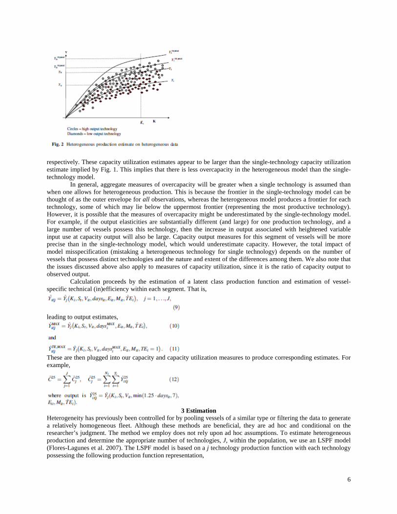
The latent class model identifies differences in output elasticities among the J production technologies, leading to curvature differences between groups of vessels. The magnitude of these differences determines the degree to which a single-technology estimate of capacity will over-/under-measure heterogeneous capacity for a given vessel. Figures 1 and 2 illustrate these differences when one assumes a single-technology versus heterogeneous technology model and the degree of over-/under-measurement of capacity generated by the single-technology model assumption, when there exists two distinct production technologies, J = 2.

Consider Fig. 1, which graphs observations of output, Y, as a function of capital, K, assuming J = 2. That is, there are two different technologies generating the data; one technology is high output (circles), while the other is low output (diamonds). Estimation of a single production function for these data might produce function Y. In this environment the two segments are evaluated as one, and the production frontier is the average of the two technologies, and it lies predominately above the low output technology (diamonds) and below the high output technology (circles). Capacity output function might be (technically efficient, with maximal primary variable input, day fished). Then single-technology capacity utilization at . Figure 2, shows the same observations but with different (heterogeneous) production functions estimated for each technology . Heterogeneity of the estimates produces a better fit for the two distinct production technologies (circles and diamonds). The technology-specific estimates of capacity utilization are for the low output (diamonds) and high output (circles) technologies,

9 There are a number of issues that must be addressed when defining capacity measures. For a more detailed discussion of these issues see Kirkley et al. (2002). 10 Alternatively, we could estimate capacity utilization as proposed by Fare et al. (1998) which is ‘unbiased’ because it is not directly influenced by technical inefficiency.

6

respectively. These capacity utilization estimates appear to be larger than the single-technology capacity utilization estimate implied by Fig. 1. This implies that there is less overcapacity in the heterogeneous model than the single-technology model.

In general, aggregate measures of overcapacity will be greater when a single technology is assumed than when one allows for heterogeneous production. This is because the frontier in the single-technology model can be thought of as the outer envelope for all observations, whereas the heterogeneous model produces a frontier for each technology, some of which may lie below the uppermost frontier (representing the most productive technology). However, it is possible that the measures of overcapacity might be underestimated by the single-technology model. For example, if the output elasticities are substantially different (and large) for one production technology, and a large number of vessels possess this technology, then the increase in output associated with heightened variable input use at capacity output will also be large. Capacity output measures for this segment of vessels will be more precise than in the single-technology model, which would underestimate capacity. However, the total impact of model misspecification (mistaking a heterogeneous technology for single technology) depends on the number of vessels that possess distinct technologies and the nature and extent of the differences among them. We also note that the issues discussed above also apply to measures of capacity utilization, since it is the ratio of capacity output to observed output.

Calculation proceeds by the estimation of a latent class production function and estimation of vessel-specific technical (in)efficiency within each segment. That is,

leading to output estimates,

These are then plugged into our capacity and capacity utilization measures to produce corresponding estimates. For example,

3 Estimation

Heterogeneity has previously been controlled for by pooling vessels of a similar type or filtering the data to generate a relatively homogeneous fleet. Although these methods are beneficial, they are ad hoc and conditional on the researcher’s judgment. The method we employ does not rely upon ad hoc assumptions. To estimate heterogeneous production and determine the appropriate number of technologies, J, within the population, we use an LSPF model (Flores-Lagunes et al. 2007). The LSPF model is based on a j technology production function with each technology possessing the following production function representation,

7

where is the appropriately dimensioned vector of marginal products. The stochastic error is composed of two components to generate the stochastic frontier model (Aigner et al. 1977; Meeusen and van den Broeck 1977) and is specified as,

The first error component, is an independently and identically distributed random variable, and

is a one-sided, non-negative vessel specific error term drawn from a truncated , with truncation below zero. Each of the j technologies share the same distributional parameters . The model is ‘ill-posed’ without this assumption (El-Gamal and Inanoglu 2005). Let and be independent and uncorrelated with the inputs measures. Given these distributional assumptions, the log-likelihood function is (Battese et al. 1989; Battese and Coelli 1995),

The EC algorithm proceeds by pre-specifying the number of production technologies within the data, J, and

then obtaining parameter estimates assuming that each agent’s contribution to the global likelihood function is the maximum joint likelihood of all their observations, , across all the J pre-specified production technologies, given

. This is specified as follows,

To determine the optimal number of latent production technologies, J*, estimates are calculated assuming a

number of different technologies, j = 1,…,J, and several model selection criteria (discussed in more detail later) are used to determine the optimal number of latent types within the data set. This method is identical to that used by Flores- Lagunes et al. (2007), but this is the first time it has been used to obtain capacity measures.

Numerical maximization of this likelihood function returns consistent estimates : Equation 15 returns consistent . The distributional assumptions in the error components imply that the distribution of

conditional on is that of a random variable truncated below zero (Battese et al. 1989; Battese and Coelli 1995), where,

8

This distribution has conditional mean (Battese and Coelli 1988),

where are the probability density and cumulative distribution of a standard normal random variable, respectively. In what follows, we will abbreviate the conditional mean as vector. Estimates are calculated by substituting for in Eqs. 17 through 19 above per (Battese and Coelli 1988) and Horrace (2005). Then in Eq. 20 is estimated by E[ui|j|ei|j]. Estimates of the efficiency probabilities, FTEi jj; are given in Horrace (2005) and are based on .

To generate output for our capacity and capacity utilization measure we use output estimates but adjusted for differing values of primary variable input (days) and for the conditional mean of efficiency, . That is,

is the efficient output at nominal inputs. Then

is inefficient output at maximal primary variable input (maximal production with deviation from the efficient frontier). Efficient output at maximal primary variable input is

These three output measure are used along with to generate capacity and capacity utilization estimates in Eqs. 2, 4, 6, and 8.

4 Data and econometric specification To illustrate our capacity and capacity utilization measures we use weekly data on catcher-processor vessels operating in the BSAI flatfish fishery for the years 1994 through 2004, inclusive. The unbalanced panel data set consists of 4,380 observations on 45 distinct vessels greater than 125 feet in length that are required to have federal fisheries observers onboard for all trips. Data obtained from the fisheries observers were merged with data from the weekly production reports filed by these vessels to create a dataset which includes vessel characteristics, the time period fished, the number of hauls made, the total length of time their gear was deployed (Duration), crew size, and a complete characterization of their catch composition. Although smaller vessels operate within the fishery, their observer data are incomplete, so they are excluded from our data (only 30% of their trips include fisheries observers). However, this is a relatively small segment in the fleet, so their exclusion should not be a problem for our analysis. The primary flatfish species caught are yellowfin sole, rock sole, flathead sole, arrowtooth flounder, flounder, rex sole, and Greenland turbot.11 Of these species, yellowfin sole comprises the largest percentage of total retained catch by the fleet, approximately 57%.12 An almost exclusively foreign group of vessels began targeting flatfish in the BSAI in mid 1950s. However, extremely high catch rates from 1959–1962 caused a dramatic decline in the fish population. With the creation of the U.S. Exclusive Economic Zone (EEZ), these foreign vessels were eventually expelled in favor of a purely domestic fishery.

Our fixed input of production, , is vessel gross-registered tonnage.13 The vector of variable inputs is crew members per week (Crew), the number of days fished during the week (days) and the amount of time the gear was

11 In addition, these vessels catch a fair amount of Pacific cod and pollock. These species compose about 8% and 6% of the total retained catch, respectively. However, we exclude them from the analysis since they are considered bycatch. 12 We focus on retained catch in our analysis instead of total catch, since we believe it more closely reflects the targeting practices of the fleet. In the case that the retained amount of yellowfin sole was zero we substituted in a value of 0.0001 metric tons to facilitate the log-transformation of the production variables. 13 We also investigated using each vessel’s horsepower but due to multicollinearity concerns it was eliminated.

9

used during the week to harvest flatfish (Duration).14 Although data on the number of weekly hauls were available, trawl duration provides a finer resolution of gear use and for parsimony (as well as collinearity concerns) we chose to use duration instead of hauls. Additionally, over the time period analyzed there was a shift in the way many of the vessels fished. Although total fishing/towing duration remained stable, vessels increased the number of hauls during the week (and thus decreased the average duration of each haul) in an attempt to decrease haul size and increase the quality of the deliverable product. It is possible that if we used the data on the number of hauls, the structural change in haul size could have impacted our ability to accurately characterize the contribution of hauls over the period and might provide misleading estimates. Dummy variables could have been used to capture such effects, but by using duration we avoid the need to estimate the additional parameters.15 The input is the month (Month) that each vessel’s fishing activity was reported in the weekly production reports. This control variable captures seasonal variation in the migration of flatfish, as well as the adverse climatic conditions present within the fishery and is a count variable indicating the month in which they fished. Earlier investigations experimented with the use of monthly dummy variables to more accurately model seasonal and climatic variation, but this rendered the empirical model intractable when the number of segments increased beyond the single-technology model.16 Finally, due to multicollinearity concerns we elected to not use information on the flatfish stock densities 17

Given our multi-species application, the production specification is the output distance function (Paul et al. 2000; Shephard 1970). In our data there are fifteen classifications for the species caught while fishing for flatfish. Because it would be difficult to estimate a fifteen species output distance function, we aggregated these classifications. We selected yellowfin sole as are our primary output because it comprises the largest portion of catch for this fleet. The other two primary species caught are rock sole and flathead sole All other species (i.e., other flatfish, rock fish, Pollock, Pacific cod, etc.) are aggregated into an ‘‘other’’ category . Our final translog specification of the output distance function is:

Our specification is precisely the output distance function of Paul et al. (2000), which imposes linear

homogeneity in outputs on the transformation function, where RHS outputs are normalized by yellowfin sole (e.g., and where the true LHS output has been multiplied by -1 to simplify interpretation of

regression coefficients. To obtain the final specification we started with the full translog functional form for the single-technology

model (J = 1) and eliminated interaction and squared terms that were highly collinear.18 The single-technology model was further refined by eliminating interaction parameters that were insignificant, using likelihood ratio tests, conditional on standard curvature conditions for the production possibilities frontier.19 We then estimated a heterogeneous model (J = 3) based on the specification we obtained for the single-technology model. Although it is possible for each segment j = 1, 2, 3 to possess its own functional form (different production inputs, say), we did not do this so that the single-technology and heterogeneous models could be directly compared. This also allows the

14 Given that both Duration and Days are definitions of time, it is important to note that the linear correlation is only 0.75, which is not as high as one may hypothesize. This is because duration is a time input relating to product quality, the captain’s ability to locate fish, and the processing technology used on board the vessel. Days, on the other hand, is a temporal input determine how long the vessel stays at sea and is influenced by the vessels hold capacity, freezing capacity and how fast the holds are filled. 15 A referee pointed out that the latent variable model assumes that vessels remain in their classes, so any vessel switching across production classes may call into question the validity the analysis. 16 Dummy variables within this framework can be problematic, for it is possible for a given dummy variable to be unvarying within a given segment. 17 Initial investigations used , but it was statistically insignificant and highly collinear with the constant term due its relative stability throughout the period studied. 18 Our criterion for this selection was a collinearity estimate of 0.9 or greater. 19 Restrictions on the coefficients were not implemented a priori, curvature restrictions were tested following estimation.

10

resulting heterogeneous model to violate production curvature restrictions in each sector j, so, in a sense, we are allowing the heterogeneous model to identify any misspecification resulting from the restriction that it be the same as the single-technology model.

Equation 21 under the single technology assumption was estimated via maximum likelihood in GAUSS. Estimation under this assumption requires simulation techniques to maximize the likelihood function in equation. This is because the likelihood function in Eq. 16 is not concave and may possess local maxima. Therefore special maximization techniques are necessary such as using repeated random starting points (Anderson and Putterman 2006), simulated annealing (Schnier and Anderson 2006), or genetic algorithms. For this study we use 500 random starting points to find the global maximum of the likelihood function, because the large number of parameters make the other techniques intractable.

5 Results, capacity and capacity utilization estimates Estimation results assuming J = 1 (first column of estimates) and J = 3 (second–fourth columns of estimates) are in Table 1.20 To determine the appropriate number of production technologies we used likelihood ratio tests, the corrected Akiake Information Criterion (crAIC), and the Bayesian Information Criterion (BIC).21 The results from these tests are in Table 2. The crAIC and BIC both increase as the number of production segments increases, suggesting that additional parameters are warranted. This is confirmed by the likelihood ratio tests conducted, which reject the null-hypothesis of reducing the number of segments from 3 to 2 and 2 to 1. In addition to estimating the crAIC and BIC we estimated the ‘‘average normalized entropy’’ (ANE) proposed by El-Gamal and Grether (1995) to test how well the segment-specific assignments fit the data. The ANE is based on the posterior segment probabilities following estimation expressed as,

where is vessel i’s likelihood function value, given parameter vector . Using these posterior probabilities the ANE test statistic is calculated as,

The ANE for our model is 0.304, which is slightly higher than those obtained by El-Gamal and Inanoglu

(2005) in their study of Turkish banking. However, this estimate is substantially below the naı¨ve estimate, which assigns equal probability to each segment. Combined these tests indicate that more than 3 production segments is appropriate, but due to the large number of parameters, we were unable to estimate a J = 4 model. However, given the small number of vessels within the fleet (45) we believe

20 Estimation results assuming J = 2 are available upon request from the author(s). 21 The 2)) and the BIC is , where G is the number of parameters estimated in the model and N is the number of vessels in the fishing fleet.

11

that the J = 3 model captures a majority of the production heterogeneity. The production elasticities assuming a single- technology and heterogeneous production technologies are in Table 3.

In Table 1, For single technology J = 1 (first column of estimates), we see that the most important production inputs are a vessel’s size (Net Tons) and the length of time a vessel deploys their gear (Duration). In addition, the complements in the multi-species production variable, , are all of the expected sign (-0.1146, -0.1764, -0.3435), and the second-order terms indicate that the presence of flathead sole, rock sole, and the other aggregate species decrease the portion of yellowfin sole caught at a decreasing rate (-0.0144, -0.0246, -0.0756, respectively). Furthermore, the production elasticities in Table 3 are all of the expected sign. Thus, our results indicate that

12

the single-technology model’s curvature conditions are consistent with economic theory. The heterogeneous production model (J = 3) in Table 1 generates distinctly different production profiles for

each technology (the second–fourth columns of estimates), with varying degrees of statistical precision. These differences are also clear in Table 4, which provides descriptive statistics for each technology. Turning back to Table 1, the first heterogeneous production technology (j = 1) contains the fewest vessels within the fleet (10), and their production is primarily determined by the level of variable inputs employed, Duration and Crew (parameter estimates of 1.8079 and 2.7112, respectively). The vessel’s size (Net Tons) and the number of days at sea within a week (Days) appear to play a much smaller role production than in the other technologies. In Table 3 we see that the elasticities of input utilization show one curvature violation in Net Tons (-0.0280) for the first technology (j = 1). However, the coefficient on Net Tons is insignificant for j = 1 in Table 1, so we can conclude that this curvature violation is insignificant. Hence, the distance function for the first production technology is well-behaved. Looking at Table 4, we can see that the first production technology (j = 1) possesses the smallest average long-run fixed input utilization measures (Length of 172.01 and Net Tons of 647.2) within the fleet and utilizes the lowest mean number of crew members (32.99). These vessels also possess a higher average percentage of other species caught (flathead sole, rock sole and other species), suggesting a less discriminatory production practice. In addition, vessels in the first technology segment fish more than any of the other technologies. On average they fish within the flatfish fishery slightly over 16 weeks a year (Weeks Fished), compared to slightly less than 5 and more than 8 for production technologies j = 2 and j = 3, respectively. Combined these results indicate that technology j = 1 consists of smaller vessels which are generalists in their production activities and part of the ‘‘core’’ fleet operating within the flatfish fishery.

The second production technology (j = 2) in Table 1 contains 16 vessels and its production is influenced more by the Month and the abundance of other flatfish species within the fishery than the other technologies. In fact, these variables have a larger marginal impact on output than changes in the quasi-fixed or variable inputs (many of which are statistically insignificant). Elasticities of production in Table 3 are all of the expected sign for j = 2. Given the lack of statistically significant quasi-fixed and variable inputs and their low level of capacity and capacity utilization (as we shall see in Tables 9 and 10), this production segment may represent a ‘‘fringe’’ technology that is either not well represented by our specification or a portion of the fleet that possesses a different targeting strategy that our model does not capture. Alternatively, this result may be driven by a reduction of statistical significance of the parameter estimates, as additional tiers are added to the latent class model. This significance reduction has been observed in latent class models of recreational climbing (Scarpa and Thiene 2005). Perhaps this segment represents the portion of the fleet that is ‘‘latent capacity,’’ that is, vessels which are not extremely active in the fishery but could become more active if it were advantageous. Support for this conjecture can be found in Table 4 for the average Weeks Fished. Vessels possessing production technology j = 2 fish less than any of the other vessels within the data set; on average they fish less than one-third of the weeks that vessels with production technology j = 1 fish. Of course the full extent of our ‘‘fringe’’ and ‘‘latent capacity’’ conjecture requires further study, but this is beyond the scope of our analysis.

The third production technology segment (j = 3) contains the largest vessels in the flatfish fishery. Per Table 4, on average these vessels are 32% and 18% longer (Length) and 85% and 83% larger (Net Tons) than

13

production technologies j = 1 and j = 2, respectively. These vessels are more selective in their production practices. On average they have the lowest catch rates for flathead sole and the largest catch rates for yellowfin sole and rock sole. In addition, these vessels are only fishing for roughly half of the time than those possessing technology j = 1 are fishing (Weeks Fished). The higher production rates for rock sole and lower average number of weeks fished by technology j = 3 suggest this technology segment is capturing the larger vessels which are more active early in the flatfish season when rock sole are predominately captured. The estimated coefficients in Table 1 indicate that technology j = 3 is somewhat similar to the single production technology J = 1. Production for these 19 vessels is primarily determined by Net Tons, and Duration (Table 1). However, the elasticities for Net Tons and Duration (see Table 3) are quite different than those in the single-technology production model, with Net Tons being larger and Duration being smaller. This production technology also possesses a curvature violation for Crew (-0.3679), however given that Crew is statistically insignificant in table 1 (0.3960), we can conclude that this is an insignificant violation and that this production technology is consistent with a well-defined output distance function.

Tables 5 through 8 contain the vessel-specific inefficiency estimates : These are used to generate the vessel-specific mean of technical inefficiency and the probability of being efficient, ; as defined in Horrace (2005) and (Flores-Lagunes et al. 2007). Table 4 contains the results under a single-technology model, sorted on : Notice that there are 45 vessels represented. In the single-technology model Vessel 40 possesses the largest probability of being the most technically efficient ( = 0.391). This is reflected in its relatively low mean of technical inefficiency (0.0648), caused by a relatively small mean (0.0307) and relatively tight variance (0.0042) prior to truncation. The results for the next two vessels in the ranking are interesting. Vessel 15 has a larger mean technical inefficiency (0.1286) than Vessel 44 (0.0982), but Vessel 15 possesses a higher probability of being efficient. This is due to the relatively large variance (prior to truncation) of Vessel 15 (0.0236). High variance prior to truncation implies a high variance after truncation (Horrace 2005), so we cannot reject the hypothesis that Vessel 15 is efficient relative to Vessel 44. This result highlights the importance of using the efficiency probabilities over (or in conjunction with) the mean of technical inefficiency, because using the mean measures alone may produce erroneous policy recommendations.22 Another interesting phenomenon occurs near the bottom of Table 5 (and 6, and 7, and 8). That is, as the gets large (ceteris paribus) it begins to dominate in the calculation of from Eq. 20, so that

Similar results are in Tables 6 through 8 but for heterogeneous production technologies. Table 6 contains the results for the 10 vessels employing production technology j = 1. Table 7 contains the results for the 16 vessels employing technology j = 2. Table 8 contains the results for the 19 vessels employing technology j = 3. In Table 6, Vessel 22 possesses the highest probability of being efficient for the first production technology. Notably, Vessel 22’s mean inefficiency estimate differs when we compare the single-technology model (0.6168 in Table 5) to the heterogeneous model (decreasing to 0.0458). A similar result arises for many other vessels possessing this production technology; the average mean inefficiency decreases from 1.0378 (single technology) to 0.6229 (heterogeneous technology). The reason is that single technology estimation forces vessels with differing technologies to be benchmarked against one another, and large differences in vessels are attributed to inefficiency differences alone (and not to technological differences). Single-technology estimation mitigates technological differences, so benchmarking reveals only differences due to inefficiency. Another interesting result is that vessel 41, the fifth most inefficient vessel in this group (0.3181), possesses the second highest rank. This result is driven by the very large , which makes it difficult to reject the hypothesis that this vessel is efficient.

In Table 7 we see that the average mean inefficiency for vessels possessing the second production technology (j = 1) decreases more than any other technology when the assumption of a single production technology is relaxed. The mean inefficiency decreases from 1.299 to 0.5166, and vessel 3, a relatively inefficient vessel in the single-technology model, has the highest mean inefficiency (0.0672) and rank. However, vessel 3’s probability (0.36735) is lower than highest ranked for the other production technologies (0.73555 in Table 5 and 0.51379 in Table 7), indicating that the probability mass for the distribution of relative efficiency is more spread out in the second technology that in the others. Notice that in Table 7 none of the vessels have a zero probability of being efficient; this is not the case for the other technologies in Tables 6 and 8. Production technology j = 3 in Table 8 parallels the

22 Another commonly used measure is the conditional expectation of , but this is simply a monotonic transformation of the conditional mean used here. Therefore, they are essentially the same for the purposes of comparative analysis and policy evaluation.

14

single-technology results of Table 5 in that vessel 40 has the smallest mean inefficiency and the highest probability rank .

15

The estimates and in Tables 5 though 8 are used to estimate capacity and capacity utilization in Tables 9 and 10 respectively based on Eqs. 2, 4, and 6. Consider the fleet capacity estimates in Table 9. The first column contains the various technologies: the single-technology model and the heterogeneous technologies identified as j = 1, j = 2, and j = 3. Consider the single-technology model in the first row. The capacity estimate ^

for the entire fleet is 898.3 thousand metric-tons of yellowfin sole over the period. This estimate assumes that each vessel is operating at mean level of inefficiency in Table 5) and that they are operating at their maximum number of days fished per week (not to exceed 7 days). We have subtracted in Table 5 from the technically efficient output in calculating this measure. Moving to the measure for the single-technology

16

model, we add the mean inefficiency back into output and the fleet capacity increases to 1,697.4 thousand metric-tons. This estimate assumes that all vessels are operating efficiently at the maximal days fished. The new measure of capacity, incorporates the probability that each boat is efficient into the capacity calculation, and it is larger than the first two estimates (2,077.1 thousand metric-tons of fish) for the single technology. The fact that

implies that high-catch vessels have a higher probability of being efficient than low-catch vessels. Continuing across the first row of Table 9 we see that the relationship is maintained for the single technology as we vary the magnitude of the days fished from 125% to 150% (This is not always true in the heterogeneous case, as we shall see.) In general, fleet capacity estimates for are approximately 1.22 times those obtained using . The imply that fleet production could be approximately doubled above

, while implies it could be more than doubled for each level of primary variable input (k = MAX, 20, 50) once efficiency is taken into account. This result is challenged when we allow for heterogeneous production technologies, however they do highlight the importance of using the estimates in capacity estimation.

The heterogeneous fleet capacity estimates in Table 8 illustrate the advantages of using heterogeneous production technologies as well as the probability scores, FTEi jj: Consider the traditional fleet capacity estimate, ^ CTE;MAX j ; for the heterogeneous production technologies. For production technologies j = 1, 2, and 3 the capacities are 457, 109, and 909.9 metric-tons of fish, respectively. These are naturally larger than the single-technology results for ^ CMAX j (349, 91.7, and 549.4 metric-tons of fish, respectively), because they place all the vessels for each technology on the efficient frontier. (This pattern is also followed for different levels of primary variable inputs, 125% and 150% of days fished.)

The truly interesting and primary results of this paper occur when we account for the probabilities of vessels being efficient in each technology, using our new capacity measure . For technology j = 1, our new capacity measure is actually lower than (391 metric-tons vs. 457 metric-tons). Apparently, for the first technology the efficient vessels tend to be those with lower catch. This is not the case for vessels using Technologies 2 and 3, where high-catch vessels tend to be more efficient (compare 261.1 to 109 and 915.6 to 909.9). In particular this phenomenon of ‘high catch boats being more efficient’ is more pronounced for technology j = 2 than for technology j = 3. Although we did not formally test it, it may be the case that the difference between 915.6 metric-tons and 909.9 metrictons for j = 3 is statistically insignificant. In that case the heterogeneous production technologies have differentiated the vessel technology into groups of vessels that are marked by (1) low-catch efficiency, (2) high-catch efficiency, and (3) medium-catch efficiency. (This pattern is also followed for different levels of primary variable inputs, 125% and 150% of days fished.)

In Table 9 the heterogeneous total estimate is simply the sum of the capacity estimates for each technology. These

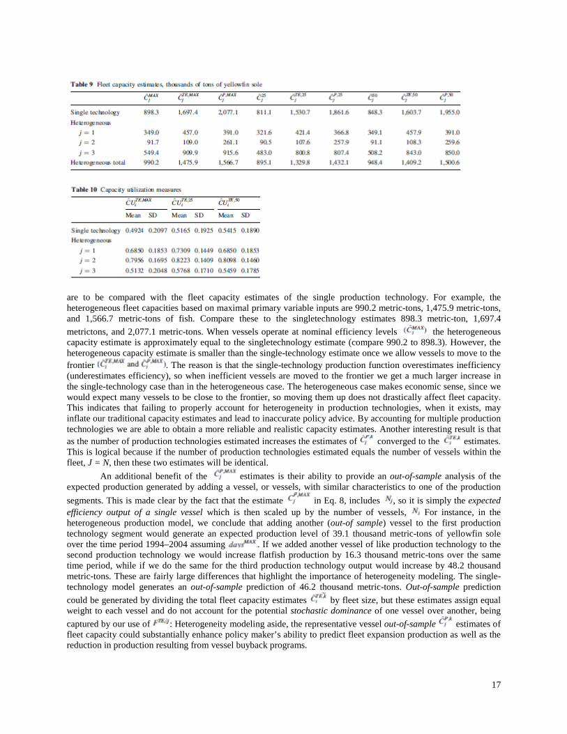
17

are to be compared with the fleet capacity estimates of the single production technology. For example, the heterogeneous fleet capacities based on maximal primary variable inputs are 990.2 metric-tons, 1,475.9 metric-tons, and 1,566.7 metric-tons of fish. Compare these to the singletechnology estimates 898.3 metric-ton, 1,697.4 metrictons, and 2,077.1 metric-tons. When vessels operate at nominal efficiency levels the heterogeneous capacity estimate is approximately equal to the singletechnology estimate (compare 990.2 to 898.3). However, the heterogeneous capacity estimate is smaller than the single-technology estimate once we allow vessels to move to the frontier . The reason is that the single-technology production function overestimates inefficiency (underestimates efficiency), so when inefficient vessels are moved to the frontier we get a much larger increase in the single-technology case than in the heterogeneous case. The heterogeneous case makes economic sense, since we would expect many vessels to be close to the frontier, so moving them up does not drastically affect fleet capacity. This indicates that failing to properly account for heterogeneity in production technologies, when it exists, may inflate our traditional capacity estimates and lead to inaccurate policy advice. By accounting for multiple production technologies we are able to obtain a more reliable and realistic capacity estimates. Another interesting result is that as the number of production technologies estimated increases the estimates of converged to the estimates. This is logical because if the number of production technologies estimated equals the number of vessels within the fleet, J = N, then these two estimates will be identical.

An additional benefit of the estimates is their ability to provide an out-of-sample analysis of the expected production generated by adding a vessel, or vessels, with similar characteristics to one of the production segments. This is made clear by the fact that the estimate in Eq. 8, includes , so it is simply the expected efficiency output of a single vessel which is then scaled up by the number of vessels, For instance, in the heterogeneous production model, we conclude that adding another (out-of sample) vessel to the first production technology segment would generate an expected production level of 39.1 thousand metric-tons of yellowfin sole over the time period 1994–2004 assuming . If we added another vessel of like production technology to the second production technology we would increase flatfish production by 16.3 thousand metric-tons over the same time period, while if we do the same for the third production technology output would increase by 48.2 thousand metric-tons. These are fairly large differences that highlight the importance of heterogeneity modeling. The single-technology model generates an out-of-sample prediction of 46.2 thousand metric-tons. Out-of-sample prediction could be generated by dividing the total fleet capacity estimates by fleet size, but these estimates assign equal weight to each vessel and do not account for the potential stochastic dominance of one vessel over another, being captured by our use of : Heterogeneity modeling aside, the representative vessel out-of-sample estimates of fleet capacity could substantially enhance policy maker’s ability to predict fleet expansion production as well as the reduction in production resulting from vessel buyback programs.

18

The vessel specific measures of capacity utilization , k = MAX, 25, 50 are in Table 10 under the assumption of single-technology and heterogeneous-technology production. Since capacity utilization is a vesselspecific measure, we simply report the means and standard deviation for the technology for each estimate. Qualitatively the estimates for the single-technology model and the third technology (j = 3) of the heterogeneous model are similar (compare 0.4924–0.5132, and 0.5165–0.5768), while there is a sizable divergence between the single technology and the second (j = 2) and third (j = 3) technology of the heterogeneous model. The increases in vessel-specific capacity utilization as we move from a single-technology model to a heterogeneous production model result from the decrease in the mean inefficiency estimates for each of the j production technologies as increasing levels of heterogeneity are incorporated. As illustrated in Figs. 1 and 2, allowing for separate production frontiers refines the mean inefficiency estimates because technically efficient output is no longer defined by the outer envelope of all the observations, but just those that are encompassed by the jth production technology. The most pronounced difference in the vessel-specific capacity utilization measures arises for second production technology (j = 2) in the heterogeneous model. As discussed earlier, the average mean inefficiency decreased from 1.299 to 0.5166 when heterogeneous production technologies were incorporated, leading each vessel to be closer to its technological frontier and to exhibit larger capacity utilization measures. These results further highlight the importance of allowing for the possibility of heterogeneous production technologies.

6 Conclusions Previous investigations of fleet capacity and vessel-specific measures of capacity utilization are based on a

single-technology production and measurement of inefficiency relative to a single production frontier. This research expands these investigations by incorporating a heterogeneous production frontier as well as using information from the complete technical inefficiency distribution. This research also enhances previous research on heterogeneous production modeling (Flores-Lagunes et al. 2007) by analyzing production in a multi-species fishery and using the information contained in the simultaneous differences of the distributions of vessel-specific technical inefficiency to construct an alternative measure of fleet capacity.

Our production technology estimates indicate that ignoring heterogeneity in production may overestimate a fleet’s capacity. Furthermore, using the complete distributional information of the fleet’s technical efficiency (captured by refines the fleet-wide estimate of capacity and suggests that traditional measures based on technically efficient production may generate unreliable capacity estimates. Combined, these results highlight the importance of accommodating production heterogeneity within fisheries—even when vessel characteristics or other measures so often used to define a ‘‘technology’’ may be quite similar—and show that additional gains may be obtained by incorporating measures on the statistical reliability of the technical efficiency scores using the second moments from the stochastic frontier models. These results should be especially beneficial for future policy development and especially for out-of-sample policy responses, which can be used to evaluate potential vessel buyback programs as well as fleet restructuring and expansion.

References Aigner DJ, Lovell AK, Schmidt P (1977) Formulation and estimation of stochastic frontier production models. J

Econom 6:21–37. doi: 10.1016/0304-4076(77)90052-5 Alvarez A, Schmidt P (2006) Is skill more important than luck in explaining fish catches? J Prod Anal 26:15–25.

doi:10.1007/ s11123-006-0002-x Anderson CM, Putterman L (2006) Do non-strategic sanctions obey the law of demand? The demand for

punishment in the voluntary contribution mechanism. Games Econ Behav 54:1–21 Battese GE, Coelli TJ (1988) Prediction of firm-level technical efficiencies with a generalized frontier production

function and panel data. J Econom 38(3):387–399. doi:10.1016/0304-4076 (88)90053-X Battese GE, Coelli TJ (1995) A model for technical inefficiency effects in a stochastic frontier production function

for panel data. Empir Econ 20:325–332. doi:10.1007/BF01205442 Battese GE, Coelli TJ, Colby TC (1989) Estimation of frontier production functions and the efficiencies of Indian

farms using panel data from ICRISAT’s village level studies. J Quant Econ 5(2):327–348 El-Gamal M, Grether D (1995) Are people bayesian? Uncovering behavioral strategies. J Am Stat Assoc 90:1137–

1145. doi: 10.2307/2291506 El-Gamal M, Grether D (2000) Are people Bayesian? Uncovering behavioral strategies using estimation

classification (EC). In: Machina M et al (eds) Preferences, beliefs, and attributes in decision making. Kluwer, New York

El-Gamal M, Inanoglu H (2005) Inefficiency and heterogeneity in Turkish banking: 1990–2000. J Appl Econom 20:641–664. doi: 10.1002/jae.835

19

Fare R, Grosskopf S, Kokkelenberg EC (1989) Measuring plant capacity, utilization and technical change: a nonparametric approach. Int Econ Rev 30:655–666. doi:10.2307/2526781

Felthoven RG (2002) Effects of the American Fisheries Act on capacity, utilization and technical efficiency. Mar Resour Econ 17(3):181–205

Felthoven RG, Paul CJM (2004) Mutli-output, nonfrontier primal measures of capacity and capacity utilization. Am J Agric Econ 86(3):619–633. doi:10.1111/j.0002-9092.2004.00605.x

Flores-Lagunes A, Horrace WC, Schnier KE (2007) Identifying technically efficient fishing vessels: a non-empty, minimal subset approach. J Appl Econ 22:729–745. doi:10.1002/jae.942

Food and Agriculture Organization (1998) Report of the technical working group on the management of fishing capacity. FAO fisheries report number 586. Food and Agriculture Organization, Rome

Garcia de Hoyo JJ, Espino DC, Toribio RJ (2005) Determination of technical efficiency of fisheries by stochastic frontier models: a case on the Gulf of Cadiz(Spain). ICES J Mar Sci 61:417–423

Greene WH (2005) Reconsidering heterogeneity and inefficiency: alternative estimators for stochastic frontier models. J Econom 126(2):269–303. doi:10.1016/j.jeconom.2004.05.003

Guyader O, Daures F, Fifas S (2004) A bioeconomic analysis of the impact of decommissioning programs: application to a limitedentry French scallop fishery. Mar Resour Econ 19:225–242

Horrace WC (2005) On ranking and selection from independent truncated normal distributions. J Econom 126:335–354. doi: 10.1016/j.jeconom.2004.05.005

Kirkley J, Squires D, Strand IE (1998) Characterizing managerial skill and technical efficiency in a fishery. J Prod Anal 9:145–160. doi: 10.1023/A:1018308617630

Kirkley J, Fare R, Grosskopf S, McConnell K, Squires D, Strand I (2001) Assessing capacity and capacity utilization in fisheries when data are limited. North Am J Fish Manag 21:482–497. doi: 10.1577/1548-8675(2001)021\0482:ACACUI[2.0.CO;2

Kirkley J, Morrison Paul C, Squires D (2002) Capacity and capacity utilization on common-pool resource industries: definition measurement and a comparison of approaches. Environ Resour Econ 22:77–97. doi:10.1023/A:1015511232039

Kirkley J, Squires D, Alam MF, Ishak HO (2003) Excess capacity and asymmetric information in developing country fisheries: the Malaysian purse seine fishery. Am J Agric Econ 85(3):647–662. doi:10.1111/1467-8276.00462

Kirkley J, Morrison-Paul C, Cunningham S, Catanzano J (2004) Embodied and disembodied technical change in fisheries: an analysis of the Sete trawl fishery, 1985–99. Environ Resour Econ 29:191–217. doi:10.1023/B:EARE.0000044603.62123.1d

Kompas T, Che TN (2005) Efficiency gains and cost reductions form individual transferable quotas: a stochastic cost frontier for the Australian South East fishery. J Prod Anal 23:285–307. doi: 10.1007/s11123-005-2210-1 188 J Prod Anal (2009) 32:173–189 123

Kompas T, Che TE, Grafton QR (2004) Technical efficiency effects of input controls: evidence from Australia’s banana prawn fishery. Appl Econ 36:1631–1641. doi:10.1080/0003684042000 218561

Meeusen W, van den Broeck J (1977) Efficiency estimation from Cobb-Douglas production functions with composed error. Int Econ Rev 18:435–444. doi:10.2307/2525757

Mistiaen JA, Strand IE (2000) Location choice of commercially fishermen with heterogeneous risk preferences. Am J Agric Econ 82:1184–1190. doi:10.1111/0002-9092.00118

Orea L, Kumbhakar SC (2004) Efficiency measurement using a latent class stochastic frontier model. Empir Econ 29(1):169–183. doi: 10.1007/s00181-003-0184-2

Orea L, Alvarez A, Morrison Paul CJ (2005) Modeling and measuring production processes for a multi-species fishery: alternative technical efficiency estimates for the northern Spain hake fishery. Nat Resour Model 18(2):183–213

Pascoe S, Coglan L (2002) The contribution of unmeasurable inputs to fisheries production: an analysis of technical efficiency of fishing vessels in the English Channel. Am J Agric Econ 84(3):585–597. doi:10.1111/1467-8276.00321

Paul CJM, Johnston W, Frengley G (2000) Efficiency in New Zealand sheep and cattle farming: the impacts of regulatory reform. Rev Econ Stat 82:325–337. doi:10.1162/003465300558713

Provencher B, Bishop RC (2004) Does accounting for preference heterogeneity improve the forecasting of a random utility model? A case study. J Environ Econ Manag 48:793–810. doi: 10.1016/j.jeem.2003.11.001

Reid C, Squires D, Jeon Y, Rodwell L, Clarke R (2003) An analysis of fishing capacity in the western and central Pacific Ocean tuna fishery and management implications. Mar Policy 27:449–469. doi:10.1016/S0308-597X(03)00065-4

20

Scarpa R, Thiene M (2005) Destination choice models for rock climbing in the Northeastern Alps: a latent class approach based on intensity of preferences. Land Econ 81(3):426–444

Schnier KE, Anderson CM (2006) Decision making in patchy resource environments: spatial misperceptions of bioeconomic models. J Econ Behav Organ 61:234–254. doi:10.1016/j.jebo. 2005.03.014

Sharma KR, Leung PS (1998) Technical efficiency of Hawaii’s longline fishery. Mar Resour Econ 13(4):259–274 Shephard RW (1970) Theory of cost and production functions. Princeton University Press, Princeton Smith MD (2005) State dependence and heterogeneity in fishing location choice. J Environ Econ Manag 50:319–

340. doi: 10.1016/j.jeem.2005.04.001 Squires D, Kirkley J (1999) Skipper skill and panel data in fishing industries. Can J Fish Aquat Sci 56:2011–2018.

doi:10.1139/ cjfas-56-11-2011 Train KE (1998) Recreation demand models with taste differences over people. Land Econ 74:230–239.

doi:10.2307/3147053 Train KE (2003) Discrete choice methods with simulation. Cambridge University Press, Cambridge, UK Viswanathan KK, Omar IH, Jeon Y, Kirkley J, Squires D, Susilowati I (2003) Fishing skill in developing country

fisheries: the Kedah, Malaysia trawl fishery. Mar Resour Econ 16:293–314 Weninger Q, Waters JR (2003) Economic benefits of management reform in the northern Gulf of Mexico reef

fishery. J Environ Econ Manag 46:207–320. doi:10.1016/S0095-0696(02)00042-6