estimating surface rupture length and magnitude of...
TRANSCRIPT
1
Estimating Surface Rupture Length and Magnitude of Paleoearthquakes
From Point Measurements of Rupture Displacement
Glenn P. Biasi and Ray J. Weldon II
February 20, 2006
Abstract.
We present a method to estimate paleomagnitude and rupture extent from measurements
of displacement at a single point on a fault. The variability of historic ruptures is
summarized in a histogram of normalized slip, then scaled to give the probability of
finding a given displacement within a rupture for any magnitude considered. The
histogram can be inverted assuming any magnitude earthquake is as likely as another,
yielding probability density functions of magnitude and rupture length for any given
displacement measurement. To improve these distributions we include a term to account
for the probability that the earthquake would cause ground rupture and two alternative
distributions of earthquake magnitude. The Gutenberg-Richter magnitude distribution
predicts shorter rupture lengths and smaller magnitudes than does a uniform distribution
where any magnitude earthquake is considered equally likely. Longer ruptures and larger
magnitudes than the uniform model are predicted by an alternative magnitude distribution
designed to return site average displacement. This model is a generalization of the
characteristic earthquake model, and reasonably describes paleoseismic findings on the
southern San Andreas fault, where slip is accommodated average displacements of a few
2
meters and earthquake recurrence times of 100-250 years. Our results should increase the
value of paleoseismic displacement measurements for hazard assessment. In particular,
they quantify probability estimates of earthquake magnitude and rupture length where
point observations of rupture displacement are available, and so can contribute to
probabilistic seismic hazard analyses.
Introduction
Paleoseismic investigations have had good success in locating and dating pre-
instrumental earthquake ruptures of the ground surface, but have been more limited in
their ability to estimate paleoearthquake magnitude or rupture length. For example, long,
well dated event chronologies at Pallett Creek and Wrightwood on the San Andreas fault
in California (Sieh et al., 1989; Fumal et al. 1993, 2002a) constrain recurrence rate and
suggest patterns in underlying fault behavior (e.g., Sieh et al., 1989; Biasi et al., 2002;
Weldon et al., 2004). However, slip estimates for individual ruptures (e.g., Sieh, 1984;
Salyards et al., 1992; Grant and Sieh, 1994; Weldon et al., 2002, 2004; Liu, et al., 2004)
have thus far contributed only a general understanding of paleoearthquake magnitude.
Because these measurements are, by their nature, point estimates of earthquake slip, it is
impossible to say whether the observed slip is representative of the average over the
entire rupture, or whether it happens to be more or less than average. Rupture length is
even less constrained than average displacement by paleoseismic studies at individual
sites. In many cases displacement at a point is assumed to be equal to the average or
maximum and rupture length is estimated using empirical regressions (e.g., Wells and
Coppersmith, 1994).
3
Where more than one paleoseismic site on a fault has been investigated, rupture lengths
have been proposed based on speculative correlation of events with overlapping age
ranges (Sieh et al., 1989; Weldon et al., 2004). Since seismic moment estimates depend
directly on rupture length and average displacement (Mo = dLW, where Mo is seismic
moment, L is the rupture length, d is the average slip, W is the rupture width, and is the
rock shear modulus), detailed chronologies recovered from the best paleoseismic sites
provide the frequency of ground rupture, but only weakly constrain paleomagnitude and
rupture length, which are of greater importance for understanding seismic hazard from
that fault.
Hemphill-Haley and Weldon (1999) proposed a method of estimating average
displacement from point displacement measurements. By a Monte Carlo method they
showed that a reasonably precise estimate of average slip could be made if five to ten
measurements of slip, preferably well distributed along of the fault, were available. The
difficulty in applying their method is that even on a relatively well studied fault such as
the southern San Andreas, very few slip estimates are available for events prior to the
most recent earthquake. Furthermore, the dates of paleoearthquakes are never precise
enough to show that the same rupture has in fact been observed at multiple sites. Chang
and Smith (2002) used an alternative means to estimate average displacement from
measurements in paleoseismic excavations. They assume that displacement profiles are
elliptical in shape, and take the lengths of the ruptures from a segmentation model of the
fault. The height of the ellipse is found using the paleoseismic displacement
4
measurement and the trench position within the segment. Average displacement and
magnitude are estimated from the resulting ellipses. It is not clear how to apply their
approach where the segmentation model is unknown or disputed, or where the elliptical
rupture shape cannot be assumed.
To develop a probabilistic estimate of magnitude given a point measure of slip, we begin
by examining the natural variability of slip along strike for historical ground-rupturing
earthquakes. Slip distributions of historic earthquakes have some common features that
allow them to be summarized in the form of an empirical probability distribution. This
empirical probability distribution is then scaled to give the forward probability of finding
a surface displacement given earthquake magnitude. By considering all possible
magnitudes we can invert these relationships for the probability of earthquake magnitude
and rupture length given a measured displacement.
Average Slip and Rupture Length Given Magnitude
Wells and Coppersmith (1994) obtained relationships of average surface displacement
and rupture length to magnitude from published reports of documented historical and
recent surface ruptures. Using data from all types of faults they found magnitude M and
surface rupture length L related by:
Equation 1: M = 5.08 + 1.16·log(L)
5
To relate magnitude and average displacement, dave, we combined the forward and
inverse relationships in Wells and Coppersmith (1994) for M given dave and dave given M:
Equation 2: M = 6.94 + 1.14·log(dave)
Equation 2 balances the misfit of M and dave data and gives a reversible relationship for M
and dave. Equations 1 and 2 were derived from observations of, respectively, 77 and 56
mapped surface ruptures ranging in magnitude from 5.6 to 8.1. We have used regressions
from Wells and Coppersmith (1994) because they are well known. In practice any
similar regressions could be used if changes are made consistently; particular choices, for
example, might be specific to the style or size of the fault under study.
Incorporating Slip Variability
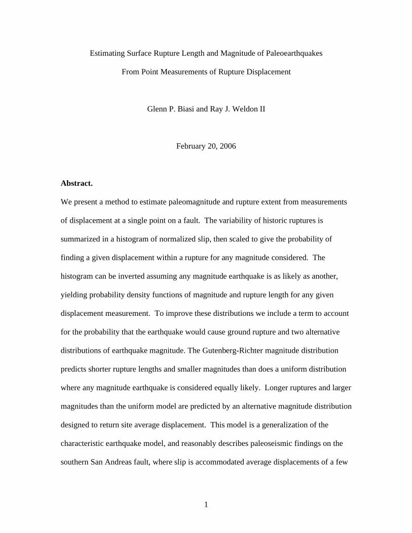
Hemphill-Haley and Weldon (1999) investigated the variability of surface slip using a
selection of earthquakes for which the displacement profile was reasonably well
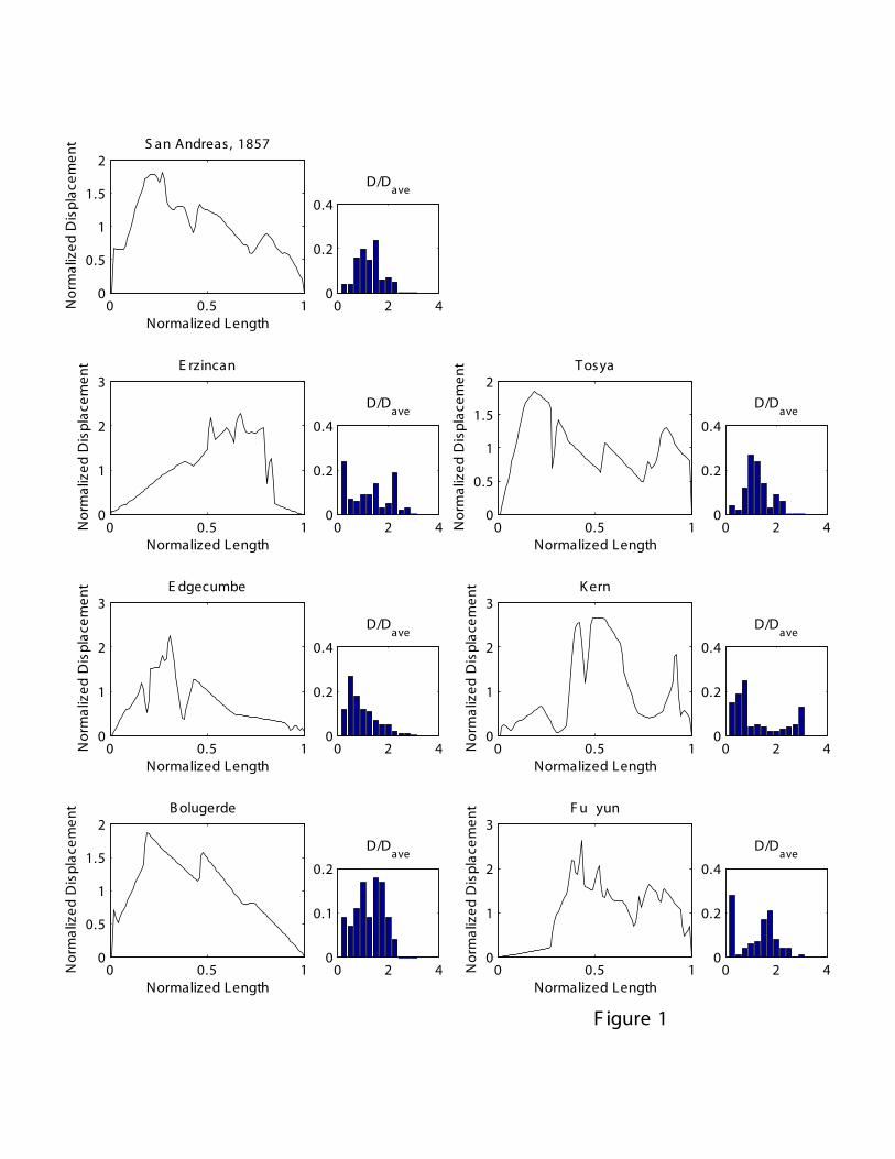
documented. Figure 1 illustrates slip variability as a function of position for several of
the mapped fault ruptures they considered. As may be seen, slip at a point commonly can
be a factor of two and the maximum a factor of three larger than the average slip along
the rupture. To characterize surface rupture variability, each rupture profile was
resampled at 1% intervals and presented in the form of a histogram (Figure 1, insets).
This has a slight smoothing effect for portions of some ruptures that have large numbers
of closely spaced displacement measurements. A key property of the histograms is that
6
they summarize surface rupture variability without specifying the spatial distribution of
individual measurements. That is, one could distribute displacements in a histogram in a
variety of ways and produce a large number of different-looking rupture profiles that
nevertheless have identical degrees of variability in d/dave. This property of histograms is
useful because in the paleoseismic context, trenching at random within the rupture and
drawing a displacement at random from the histogram are mathematically equivalent.
While individual slip distributions can be quite variable, Hemphill-Haley and Weldon
(1999) noted two important features about them. First, slips tend to be as variable for
small earthquakes as for large ones. That is, one could not tell from the shape of a slip
distribution alone whether a large or small earthquake was plotted. Second, all
distributions necessarily have ends and tend to taper to small slip offsets as the ends are
approached. This suggests an approximate shape upon which the variability is expressed.
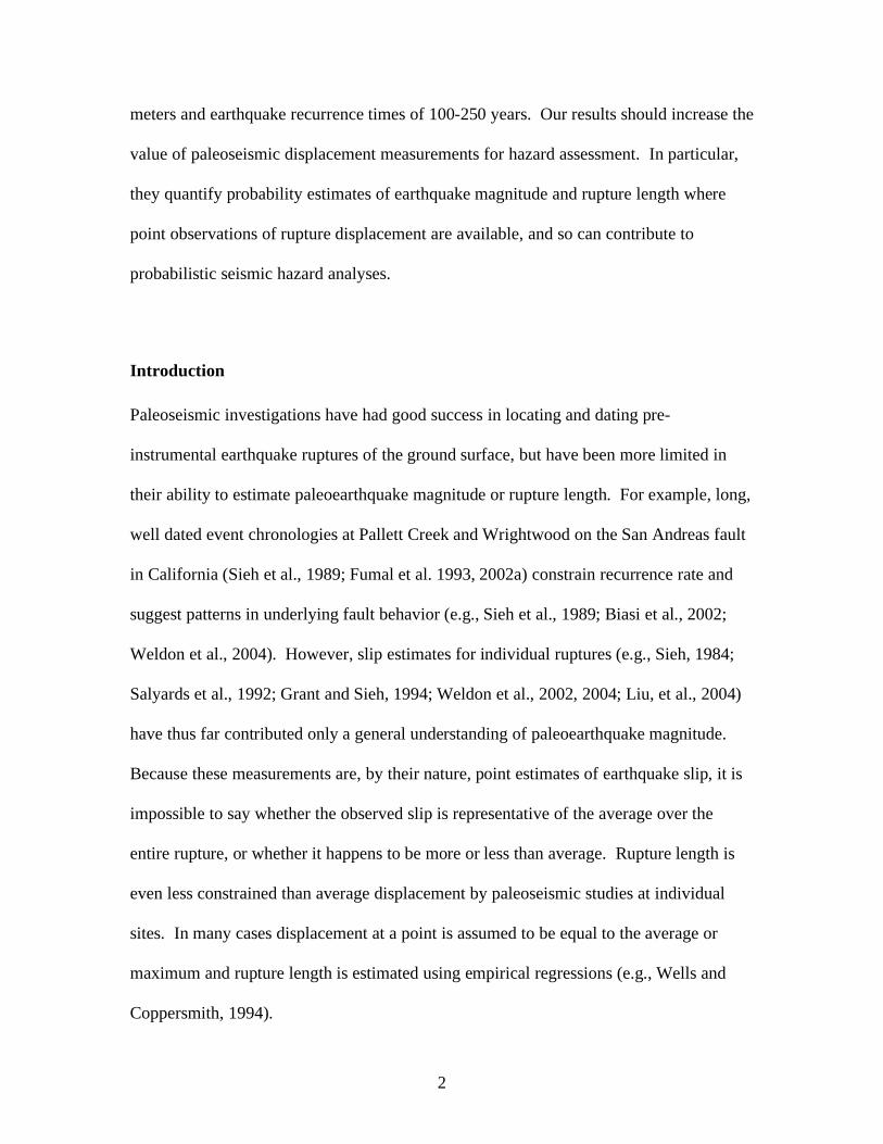
Hemphill-Haley and Weldon (1999) used these qualities as a means of combining slip
distributions of small and large earthquakes. They normalized each slip distribution by
the average displacement for that event, and the rupture length by the total observed
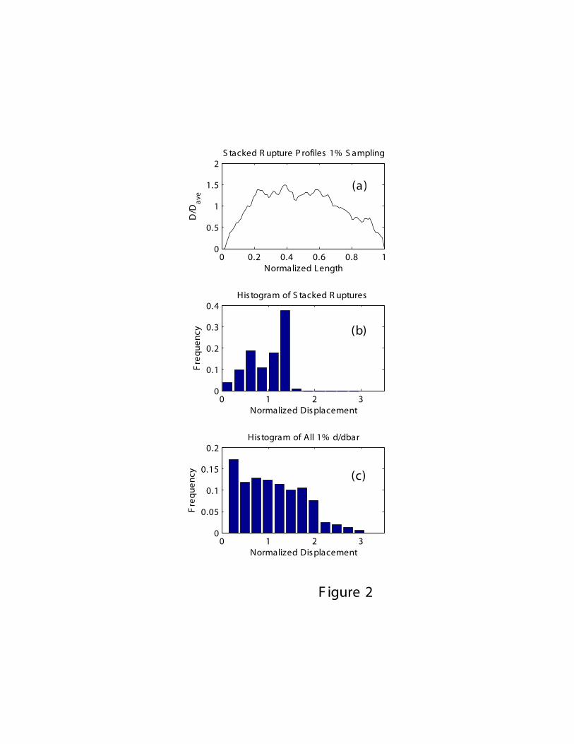
length. From these, two stacked distributions were developed (Figure 2). When the
normalized rupture profiles themselves are stacked (Figure 2a), the average rupture
profile shape includes a nearly flat central part amounting to approximately one third of
the total slip length and tapers on each end. In detail the shape of the average rupture
profile depends to a minor degree on how each rupture is included – i.e., on which end is
given the normalized length of 0 or 1 (see Hemphill-Haley and Weldon, 1999, for a
discussion). However, in any construction the average shape is far less variable than any
7
contributing rupture. Like the averaged rupture profile, its histogram (Figure 2b) has too
little variability to represent a likely result from field mapping.
On the other hand, when the individual histograms themselves are stacked (Figure 2c),
variability is preserved. Stacking is equivalent to (and accomplished by) making a single
histogram of all the d/dave measurements from contributing ruptures, then making it a
probability distribution by dividing by the total number of measurements. This process
preserves extreme normalized values (e.g., d/dave = 3), for example, but weights them by
their relative frequency of occurrence in the contributing ruptures. Unlike the averaged
rupture profile (Figures 2a, b), the averaged histogram can be used for inverting rupture
variability because it retains the full variability of the input ruptures.
Probability of Slip Given Magnitude
A key to the Bayesian inversion of slip observations for earthquake magnitude and
rupture length is the observation that, if given a unit area, the histograms of individual
earthquake ruptures (Figure 1) may be interpreted as probability density functions for slip
during those earthquakes. Probability of slip in a given range around a given
displacement can be found by integrating the appropriate portion of the histogram. This
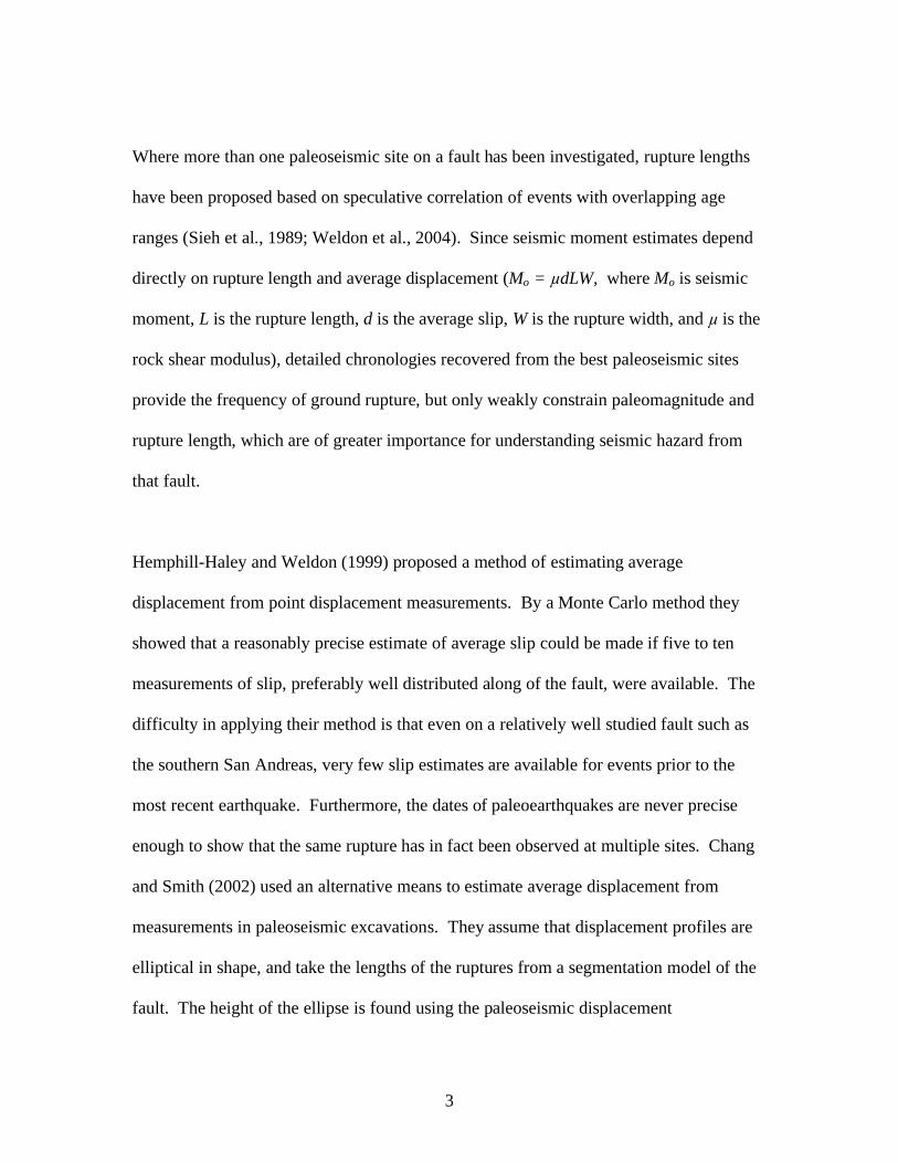
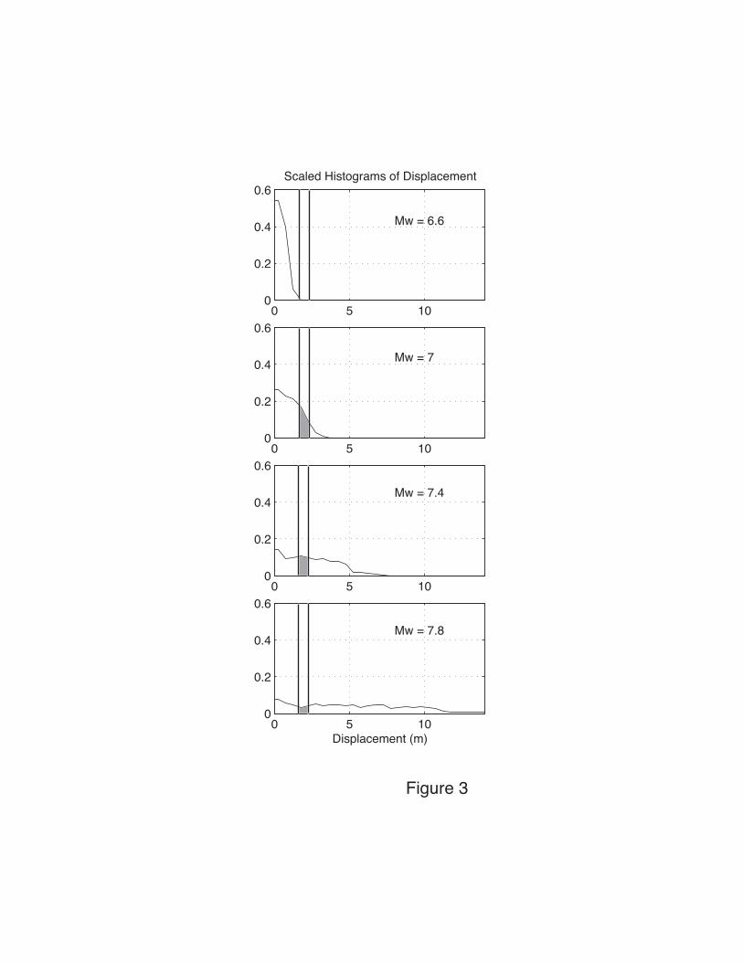
interpretation also applies to the average histogram (Figure 2c). If Equation 2 is then
used to scale the histogram in Figure 2c it becomes a probability density function for
surface displacement given magnitude, p(dobs|M(dave)). Probability density functions
p(d|M) are shown in Figure 3 for example magnitudes. The curves in Figure 3 amount to
8
predictions of surface displacement and variation based on the combined experience of
the thirteen contributing ruptures.
Bayesian Inverse for Magnitude Given Slip.
Bayes Theorem allows the slip variability p(d|M) to be inverted for the probability
distribution of earthquake magnitude given an observed displacement, p(M|dobs).
Bayes Theorem may be stated as,
Equation 3 p(M|dobs) = p(M)[p(dobs|M) /P(dobs)].
Briefly, Equation 3 revises p(M), the a priori distribution of earthquake of magnitude M,
by its likelihood in light of a paleoseismic displacement observation. The distribution of
magnitudes is unknown, but has basic limits. For the moment, we assume that any
magnitude in the range M 6.6 to M 8.1 in 0.1 magnitude unit increments is equally likely
to produce ground rupture and thus p(M) is uniformly distributed on this range. We
explore the effects of the range and shape of p(M) in later sections.
To estimate the relative weighting of individual magnitudes in Equation 3, the slip
histogram from Figure 2c is scaled for each by the average displacement predicted by
Equation 2 (Figure 3). The probability that magnitude Mi caused observed slip dobs is the
ratio of the area in the ith
histogram near dobs, P(d: d- dobs d+ |Mi) to the total area
9
in all the histograms in this displacement range. The relative likelihoods among
candidate magnitudes is given by the area of each as their fraction of the total. P(dobs) in
Equation 3 is that total area. The shaded vertical bar in Figure 3 corresponds to an
example slip of d = 2 ± 0.25 meters. For each magnitude, prior distribution p(M) then
multiplies the fraction to yield p(M|dobs).
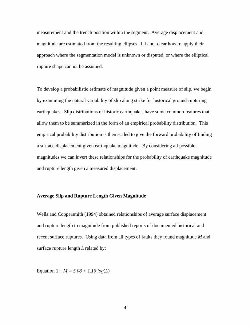
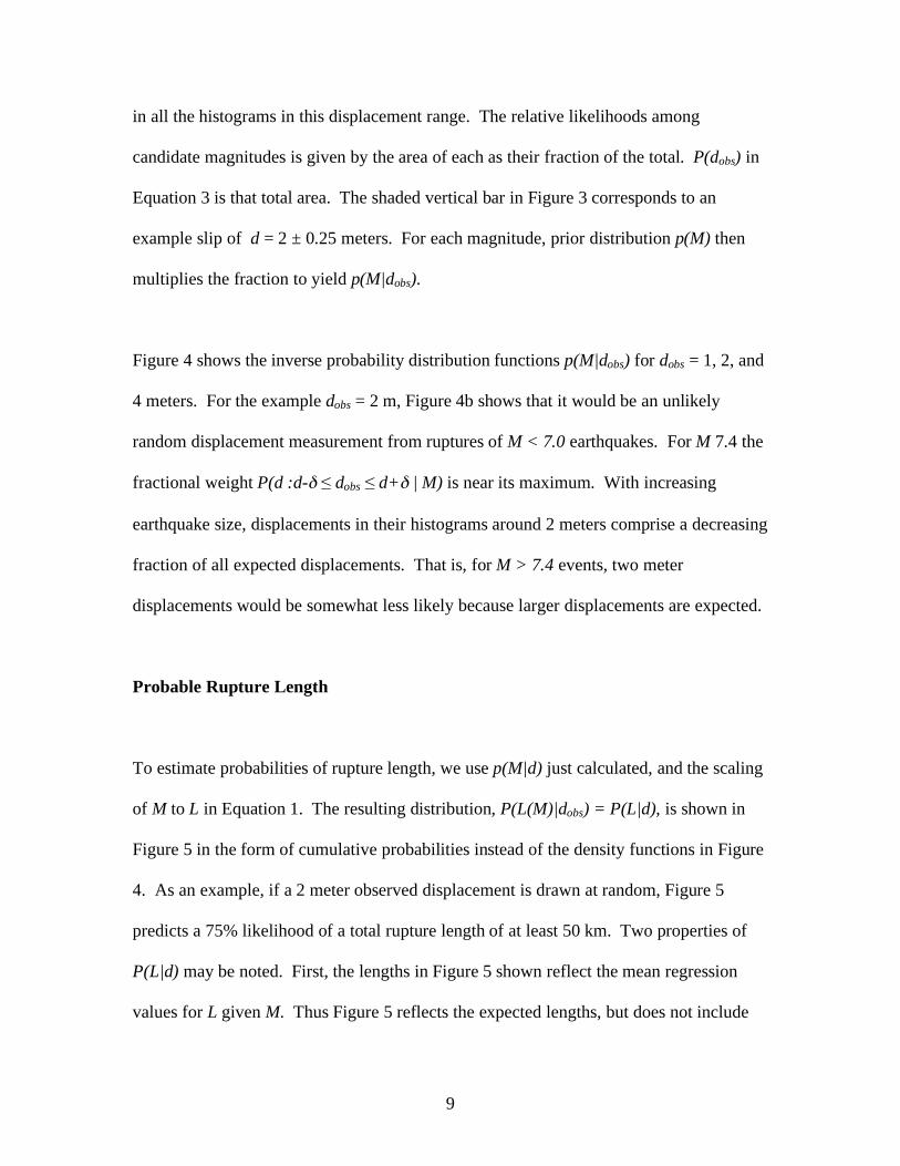
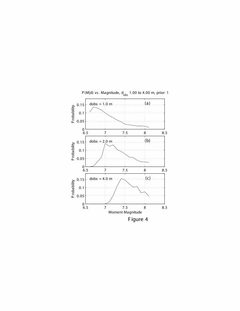
Figure 4 shows the inverse probability distribution functions p(M|dobs) for dobs = 1, 2, and
4 meters. For the example dobs = 2 m, Figure 4b shows that it would be an unlikely
random displacement measurement from ruptures of M < 7.0 earthquakes. For M 7.4 the
fractional weight P(d :d- dobs d+ | M) is near its maximum. With increasing
earthquake size, displacements in their histograms around 2 meters comprise a decreasing
fraction of all expected displacements. That is, for M > 7.4 events, two meter
displacements would be somewhat less likely because larger displacements are expected.
Probable Rupture Length
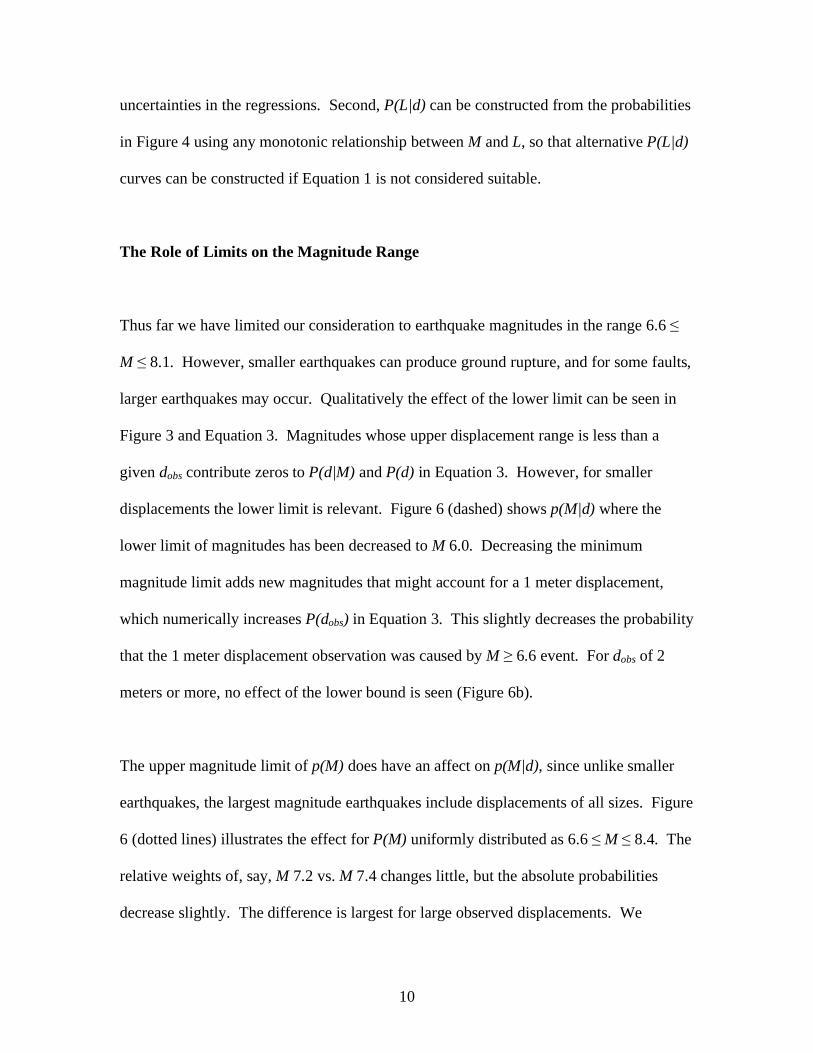
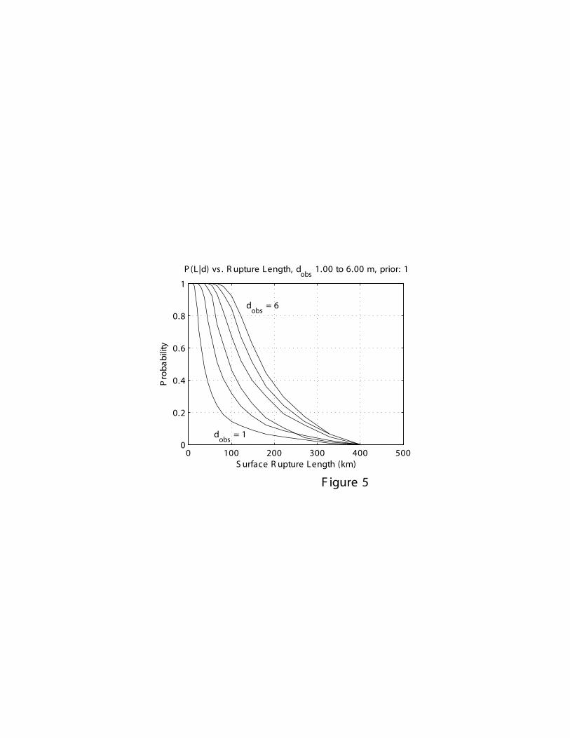
To estimate probabilities of rupture length, we use p(M|d) just calculated, and the scaling
of M to L in Equation 1. The resulting distribution, P(L(M)|dobs) = P(L|d), is shown in
Figure 5 in the form of cumulative probabilities instead of the density functions in Figure
4. As an example, if a 2 meter observed displacement is drawn at random, Figure 5
predicts a 75% likelihood of a total rupture length of at least 50 km. Two properties of
P(L|d) may be noted. First, the lengths in Figure 5 shown reflect the mean regression
values for L given M. Thus Figure 5 reflects the expected lengths, but does not include
10
uncertainties in the regressions. Second, P(L|d) can be constructed from the probabilities
in Figure 4 using any monotonic relationship between M and L, so that alternative P(L|d)
curves can be constructed if Equation 1 is not considered suitable.
The Role of Limits on the Magnitude Range
Thus far we have limited our consideration to earthquake magnitudes in the range 6.6
M 8.1. However, smaller earthquakes can produce ground rupture, and for some faults,
larger earthquakes may occur. Qualitatively the effect of the lower limit can be seen in
Figure 3 and Equation 3. Magnitudes whose upper displacement range is less than a
given dobs contribute zeros to P(d|M) and P(d) in Equation 3. However, for smaller
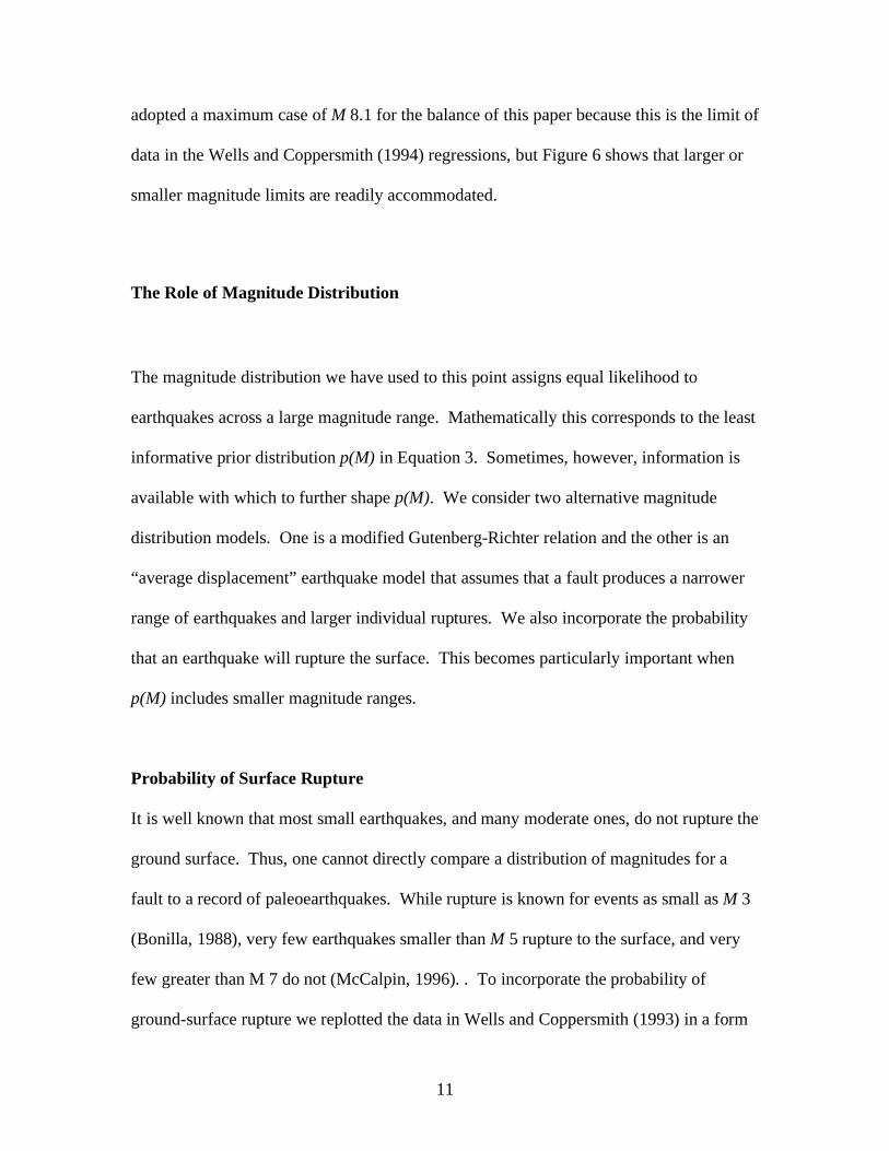
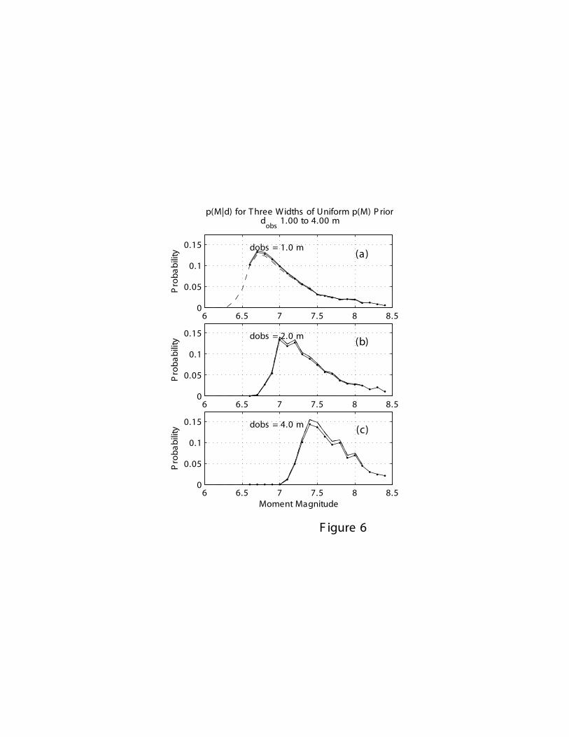
displacements the lower limit is relevant. Figure 6 (dashed) shows p(M|d) where the
lower limit of magnitudes has been decreased to M 6.0. Decreasing the minimum
magnitude limit adds new magnitudes that might account for a 1 meter displacement,
which numerically increases P(dobs) in Equation 3. This slightly decreases the probability
that the 1 meter displacement observation was caused by M 6.6 event. For dobs of 2
meters or more, no effect of the lower bound is seen (Figure 6b).
The upper magnitude limit of p(M) does have an affect on p(M|d), since unlike smaller
earthquakes, the largest magnitude earthquakes include displacements of all sizes. Figure
6 (dotted lines) illustrates the effect for P(M) uniformly distributed as 6.6 M 8.4. The
relative weights of, say, M 7.2 vs. M 7.4 changes little, but the absolute probabilities
decrease slightly. The difference is largest for large observed displacements. We
11
adopted a maximum case of M 8.1 for the balance of this paper because this is the limit of
data in the Wells and Coppersmith (1994) regressions, but Figure 6 shows that larger or
smaller magnitude limits are readily accommodated.
The Role of Magnitude Distribution
The magnitude distribution we have used to this point assigns equal likelihood to
earthquakes across a large magnitude range. Mathematically this corresponds to the least
informative prior distribution p(M) in Equation 3. Sometimes, however, information is
available with which to further shape p(M). We consider two alternative magnitude
distribution models. One is a modified Gutenberg-Richter relation and the other is an
“average displacement” earthquake model that assumes that a fault produces a narrower
range of earthquakes and larger individual ruptures. We also incorporate the probability
that an earthquake will rupture the surface. This becomes particularly important when
p(M) includes smaller magnitude ranges.
Probability of Surface Rupture
It is well known that most small earthquakes, and many moderate ones, do not rupture the
ground surface. Thus, one cannot directly compare a distribution of magnitudes for a
fault to a record of paleoearthquakes. While rupture is known for events as small as M 3
(Bonilla, 1988), very few earthquakes smaller than M 5 rupture to the surface, and very
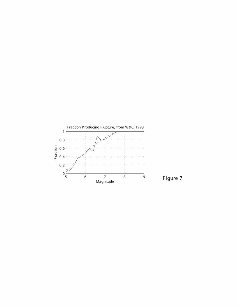
few greater than M 7 do not (McCalpin, 1996). . To incorporate the probability of
ground-surface rupture we replotted the data in Wells and Coppersmith (1993) in a form
12
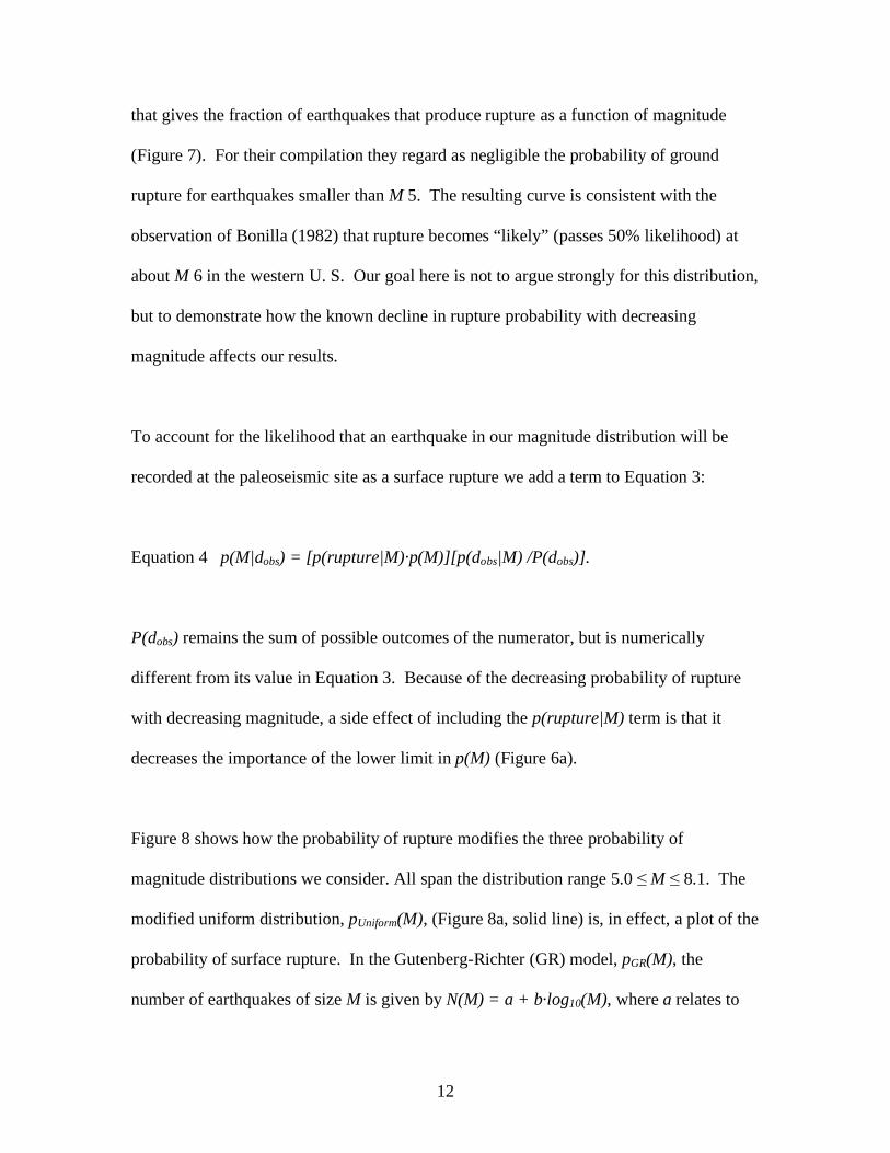
that gives the fraction of earthquakes that produce rupture as a function of magnitude
(Figure 7). For their compilation they regard as negligible the probability of ground
rupture for earthquakes smaller than M 5. The resulting curve is consistent with the
observation of Bonilla (1982) that rupture becomes “likely” (passes 50% likelihood) at
about M 6 in the western U. S. Our goal here is not to argue strongly for this distribution,
but to demonstrate how the known decline in rupture probability with decreasing
magnitude affects our results.
To account for the likelihood that an earthquake in our magnitude distribution will be
recorded at the paleoseismic site as a surface rupture we add a term to Equation 3:
Equation 4 p(M|dobs) = [p(rupture|M)·p(M)][p(dobs|M) /P(dobs)].
P(dobs) remains the sum of possible outcomes of the numerator, but is numerically
different from its value in Equation 3. Because of the decreasing probability of rupture
with decreasing magnitude, a side effect of including the p(rupture|M) term is that it
decreases the importance of the lower limit in p(M) (Figure 6a).
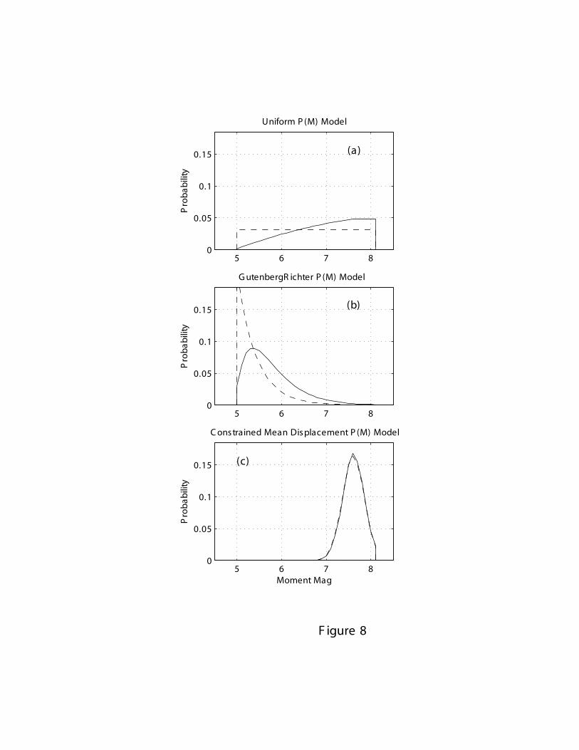
Figure 8 shows how the probability of rupture modifies the three probability of
magnitude distributions we consider. All span the distribution range 5.0 M 8.1. The
modified uniform distribution, pUniform(M), (Figure 8a, solid line) is, in effect, a plot of the
probability of surface rupture. In the Gutenberg-Richter (GR) model, pGR(M), the
number of earthquakes of size M is given by N(M) = a + b·log10(M), where a relates to
13
fault productivity and b is typically about 1.0. This model predicts 10 times more
earthquakes of M 6.0 than M 7.0. The exponential increase in the number of earthquakes
with decreasing magnitude is balanced by the declining probability of rupture, so that
pGR(M) peaks at about M 5.4 and decreases to zero by M 5 (Figure 8b, solid line). The
GR model exerts strong a priori influence on estimates of magnitude and rupture length.
Compared to a uniform model, using the Gutenberg-Richter model in Equation 4 raises
the relative probability that a given displacement observation came from an above
average slip point of a smaller magnitude earthquake.
The average displacement model, pAD(M), is intended to model the paleoseismic case
where a comparatively small number of ruptures account for a large total displacement.
The sizes of individual earthquake may not be constrained, but the average displacement
over many events is known from the recurrence time and the geologic or geodetic
average slip rate for the fault at the location of interest. The “characteristic earthquake”
model (Schwartz and Coppersmith, 1984) is an extreme form of the pAD(M) model. To
construct pAD(M) an average displacement is selected and a standard deviation is
estimated consistent with the width of the scatter in the data of Wells and Coppersmith
(1994) for that magnitude. We then convert this displacement distribution into a
magnitude distribution using the displacement-magnitude scaling relationship in Equation
2. (This application motivated our modification of Equation 2 from the original result of
Wells and Coppersmith, 1994).
14
To illustrate the average displacement model we use a mean displacement of 4.3 meters
(Figure 8c). The value of 4.3 m is based on the 135 year average recurrence interval of
ground rupturing earthquakes estimated from the Pallett Creek paleoseismic site (Sieh et
al., 1989; Salyards et al, 1992; Biasi et al., 2002), and a slip rate of ~32 mm/yr. The
Pallett Creek average displacement estimate is based on a ten earthquake record, so one
would have to claim that several ground-rupturing earthquakes were not detected to
seriously change it. The upper range was truncated at M 8.1 to facilitate direct
comparison with the other p(M) models. The shape of pAD(M) in Figure 8c is intended to
illustrate the consequences of the present paleoseismic data; in detail we cannot show that
this pAD(M) model is necessarily unique or even optimal. In principle one could construct
an empirically shaped distribution of displacements if a sufficient number of
measurements were available for the site of interest.
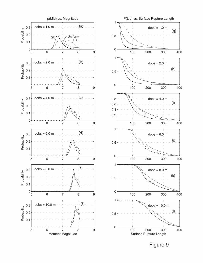
The resulting p(M|dobs) and P(L|dobs) distributions for the three p(M) models are shown in
Figure 9. Each p(M) model has different properties. For example, the GR p(M) model
includes more small earthquakes, and so predicts that one should rarely expect a slip of
one meter to have been caused by an earthquake above the low M 7 range (Figure 9a).
For all dobs values the mean estimated earthquake magnitude is smaller for the GR model
than the uniform, although the difference decreases with increasing dobs (Figure 9b-f).
The average displacement p(M) model also strongly shapes consequent p(M|dobs) and
p(L|dobs) distributions (Figure 9, dashed). For small dobs, the rarity of smaller rupture-
producing earthquakes in pAD(M) means that even when observed displacements are
small, they are attributed to mid-M 7 and larger earthquakes. This behavior is opposite to
15
that of the GR model, corresponding to the opposite relative abundances of moderate
earthquakes. At the largest magnitudes and displacements, all p(M|dobs) curves are
affected by the data-derived irregularities in the large d/dave tail of p(d|M) histograms
(Figures 2c and 3).
Probabilities of length given observations of displacement P(L|dobs) are plotted in the
right-hand column of Figure 9 for each of the p(M) models. P(L|dobs) is calculated from
the cumulative probability of p(M|dobs), and scaled horizontally to length through
Equation 1. The differences between p(M) models are most evident for small values of
dobs. The GR model predicts shorter rupture lengths for any given displacement
observation because, in the pool of all possible earthquakes that could account for dobs,
there is a higher fraction of smaller earthquakes, and therefore of shorter lengths. By
contrast, the average displacement model has a smaller fraction of smaller events, so if
one does observe a 1 m ground-rupture displacement, it is considered more likely to be a
small displacement observation from a larger earthquake. At first it may be
counterintuitive that any model would predict a median rupture length of 90 km from a 1
m displacement observation, but it is not unreasonable for a fault where the AD model
would apply. Returning to the Pallett Creek example, if the count of ground ruptures is
approximately complete, the resulting 4.3 m average displacement means that each 1 m
displacement must be balanced by another with 7.6 m. One consequence of this balance
is to push upward the probability that the 1 m displacement is a smaller displacement
observation from a larger earthquake, with the median length found to be ~90 km. The
difference among lengths predicted from larger displacements decreases with increasing
16
dobs. At largest dobs values, limiting the upper magnitude to M 8.1 has the effect of
increasing the relative probability that a large dobs came from an exceptional section of a
smaller earthquake.
Discussion
Hemphill-Haley and Weldon (1999) inferred that surface displacements are usefully
similar when normalized by average displacement and surface rupture length. This
underlies the scaling employed in Figure 3 and all subsequent results. The variability of
rupture displacements at distinct magnitude levels might be tested if a much larger
ground rupture set were consulted. Histograms developed by magnitude might be
constructed instead of the scaling method of Figure 3. Another obvious refinement to our
results would be to separate a larger data set by tectonic setting or fault type. The
average histogram we used includes earthquake ruptures from all the principal tectonic
styles, and reasonably represents the individuals from which it was compiled.
Differences among strike-slip, reverse, and normal faults suggest that factors such as the
continuity of rupture and the ratio of the average displacement to the maximum may vary
systematically. For example, McCalpin and Slemmons (1998) found differences among
fault types when maximum displacement was used to scale ruptures. It remains to be
seen, however, just how important likely differences between fault types or environments
are for estimates of magnitude and length.
17
The inversion for p(M|d) and p(L|d) assume that the observed displacement is drawn at
random from within the rupture. This assumption is designed for the case where little is
known about the extent of surface rupture for the earthquakes under study. For example,
this assumption could be applied on the southern San Andreas fault to nine of the most
recent ten events at Pallett Creek, five of the most recent six in the Carrizo Plain (Liu et
al., 2004), and all of the most recent events at the Thousand Palms Oasis (Fumal et al.,
2002b). In some cases, however, the observed displacement may be known to be
exceptional, especially when investigating the most recent event on a fault. Large
displacements in a surface rupture withstand erosion longer and have a larger probability
of discovery in the course of detailed mapping of the fault. For the same reasons one
may not sample the ends of a rupture because the surface evidence has eroded away and
only subsurface evidence remains. Choosing a trench site because a scarp is especially
well expressed, or avoiding a location because no rupture evidence remains both will tend
to bias the displacement measurement toward larger values (Stirling et al., 2002). Note,
however, that both conditions amount to stronger prior knowledge about the paleorupture
than we assume in our formulation. Sampling can also be biased toward smaller slip
observations. This can occur at splays and step-overs where rupture displacement trails
off on one fault trace and is taken up on a parallel trace some distance away. Such step-
over features tend to create structural basins (e.g., sag ponds) favorable for sedimentation
and stratigraphic preservation (e.g., Hog Lake, Rockwell et al., 2003; Pallett Creek, Sieh,
1984; Frazier Park, Lindvall et al., 2002). For both cases, displacement measurements
over multiple slips and comparision to the likely average displacement will help.
Deciding that an observed displacement is greater or less than average for a rupture is,
18
ultimately, a professional judgment, and can affect probability estimates of magnitude
and rupture length.
Figure 1 suggests another way, in principle, by which to find a biased observation of
displacement. If it is known that the observation comes from one or other end of a
rupture, then smaller than average displacements may be expected. Chang and Smith
(2002) applied this idea in their study of the Wasatch Frontal fault system to estimate
paleomagnitudes from trench offsets. If the segment boundaries are known, and ruptures
honor the boundaries, adjustment of the observed displacements might be entertained.
Bayesian inverse models characteristically depend on the prior model to be shaped by the
data. The uniform prior p(M) model is usually considered to be the least informative
prior upon which to apply p(d|M). Mathematically the information in pUniform(M) is in
where one sets the ends. By including the probability of rupture (Figure 7), the lower
magnitude bound can be arbitrarily small. The upper magnitude bound (Figure 8a) has
little effect on the relative weight among smaller events. A uniform prior model that
spans the range of conceivable magnitudes might be applied on a fault about which little
is known, or where one is reluctant to assert additional information.
The Gutenberg-Richter model was developed to characterize seismicity in a region, and
includes an exponential increase in the number of smaller earthquakes. Even when the
probability of rupture is included, pGR(M) still predicts that most ground ruptures are
caused by the relatively smaller end of the magnitude range (Figure 8b). In the field,

19
assuming this model will have the effect of preferentially attributing rupture to relatively
smaller earthquakes, just because a greater fraction of all ruptures one might find are in
this magnitude range. The applicability of the model to individual faults has been
debated (Wesnousky, 1994; Scholz, 2002; Stirling et al., 1996), but nevertheless the GR
p(M) model might be a good choice when studying a region about which little is known.
The average displacement p(M) model (Figure 8c) also strongly shapes p(M|d) and
P(L|d). Applied to the San Andreas fault, however, we would argue that it is informed, at
least, by paleoseismic data obtained on the fault. The features of a paleoseismic record
most important for the average displacement model are its completeness of event
detection and the approximate date of the oldest event in the complete section. From the
Carrizo Plains to Indio (Grant and Sieh, 1994; Liu et al., 2004; Sieh et al. 1989; Fumal et
al. 2002a; Seitz et al. 1997; Yule and Howland, 2001; Fumal et al., 2002b; Sieh, 1986)
records interpreted to be fairly complete require average slips of a few meters per event
based on direct measurement or on the estimated recurrence intervals and the geologic or
geodetic slip rates. Thus the data require some sort of enforcement of an average slip and
thus a shape on pAD(M). Figure 8c shows that a strong penalty against M < 7.2 events is
needed to achieve average displacements of 4 meters or more. Better ideas on the precise
shape of the average displacement model may emerge, but even in the form of Figure 8c
it bears a closer resemblance to displacements required by the long paleoseismic records
on the San Andreas fault than either of the other p(M) models considered.
The average displacements implied by the p(M) models in Figure 8 contribute to which
may be preferred in a given situation. Average displacements are computed by summing
20
the probability of each magnitude times the displacement predicted from Equation 2.
Average displacements for the models of Figure 8, after the correction for probability of
rupture, are 2.65, 0.23, and 4.3 meters for the uniform, GR, and average displacement
models, respectively. The average displacement for the pUniform(M) model is most
affected by the upper magnitude bound. The Gutenberg-Richter average displacement is
least affected by the choice of a maximum magnitude because while rupture displacement
increases exponentially with magnitude (under the regression), the frequency of the
largest events decreases exponentially, so that the average displacement increases only
very slowly with the maximum magnitude. The average displacement models are built to
match site average displacement, and thus have to be evaluated by other criteria. Some
modification of the probability of rupture (Figure 7) might be argued on the grounds that
small displacements are less likely to be detected with paleoseismic methods, but
reasonable modifications are unlikely to change the general properties of the p(M)
models.
An immediate application for the p(M|d) and p(L|d) relationships in Figures 4 and 5 is to
help quantify certain elements of probabilistic seismic hazard analysis. For example,
logic tree assessments typically recognize a range of magnitudes. Where rupture
displacement information is available, the present results may be applied directly or with
suggested adjustments to quantify branch weights for magnitude and rupture length.
Conclusions
21
We show that probabilities of magnitude and surface rupture length can be developed
given a displacement measurement from paleoseismic excavation. Rupture variability is
summarized in a histogram that captures the degree of variability without prescribing
how it is distributed within a rupture. The observation that sampling at random from a
histogram of slip measurements is equivalent to sampling in a random location within the
corresponding rupture makes the inversion possible.
The average histogram of variability can be interpreted as the probability of displacement
given magnitude once it is scaled using a regression of average displacement versus
magnitude. Bayes Theorem allows us to invert p(dobs|M) for probabilities of earthquake
magnitude and rupture length given point observations of displacement, p(M|d) and
p(L|d), respectively. These distributions are less than the explicit answer to the question,
“How big was it?”, but they do quantify the probability of any magnitude range or length
estimate given a rupture displacement measurement. These are common input
parameters to probabilistic seismic hazard analysis.
The inverse probabilities for magnitude and length do depend on the magnitude
distribution model assumed as an input. We analyze three, the uniform, Gutenberg-
Richter, and average displacement models after modifying each to account for the
decreasing probability of rupture with decreasing magnitude. The least restrictive form
of p(M), the uniform distribution, assumes any magnitude is as likely as another. The
Gutenberg-Richter magnitude distribution is a strong a priori assertion about p(M), and
biases magnitude and length probability estimates toward smaller values. Average
22
displacement for the GR model depends little on the maximum magnitude chosen
because the presumed exponential increase in displacement is offset by an exponential
decrease in probability of occurrence. The average displacement model is formed using a
range and probability of magnitudes designed such that sampling from it returns an
average slip, such as may be inferred from the recurrence interval and the geologic or
geodetic slip rate on the fault. Slip-per-event is only loosely constrained, distinguishing
it in that respect from the characteristic earthquake model. For faults with large average
displacements, this model predicts that even modest rupture displacement observations of
a meter or two are likely to correspond to ruptures over 100 km in length. Virtually all
paleoseismic studies of the southern San Andreas fault indicate that slip is accommodated
by relatively infrequent ruptures with a few meters average slip. Thus, among the models
considered, some form of average displacement model is preferred for the southern San
Andreas fault.
Captions
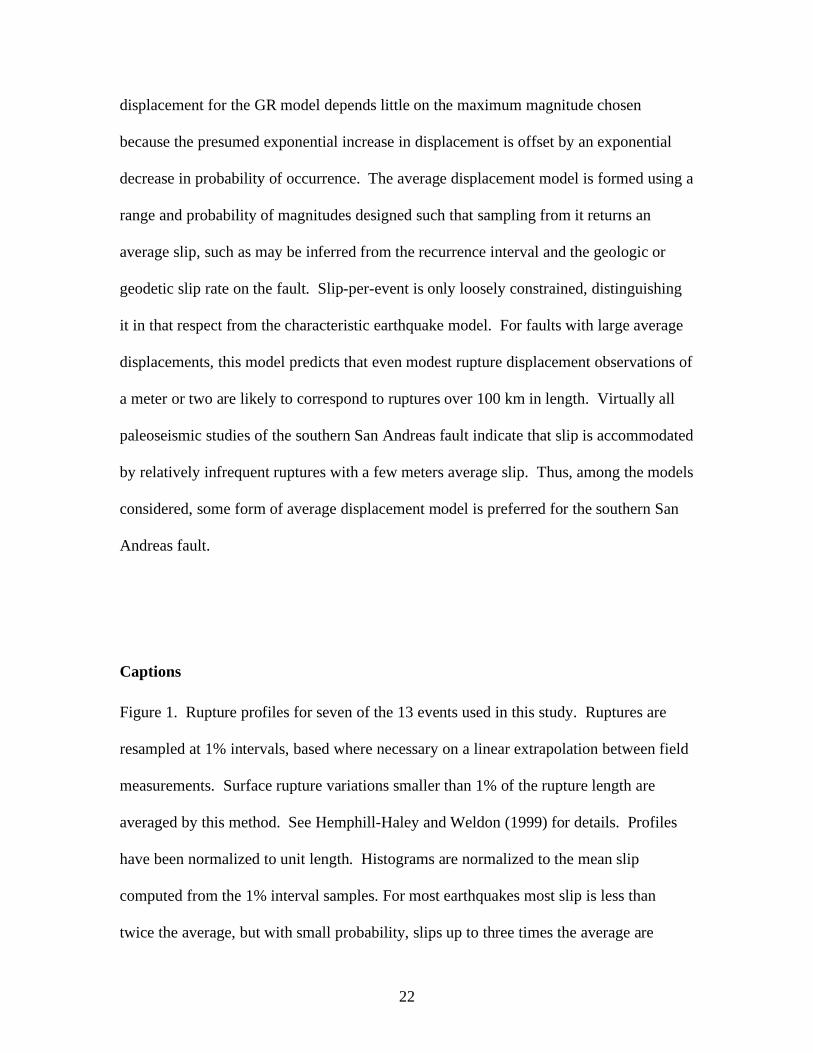
Figure 1. Rupture profiles for seven of the 13 events used in this study. Ruptures are
resampled at 1% intervals, based where necessary on a linear extrapolation between field
measurements. Surface rupture variations smaller than 1% of the rupture length are
averaged by this method. See Hemphill-Haley and Weldon (1999) for details. Profiles
have been normalized to unit length. Histograms are normalized to the mean slip
computed from the 1% interval samples. For most earthquakes most slip is less than
twice the average, but with small probability, slips up to three times the average are
23
observed. The 1% resampled rupture profiles used in this work and original references
from Hemphill-Haley and Weldon (1999) are available in an electronic supplement.
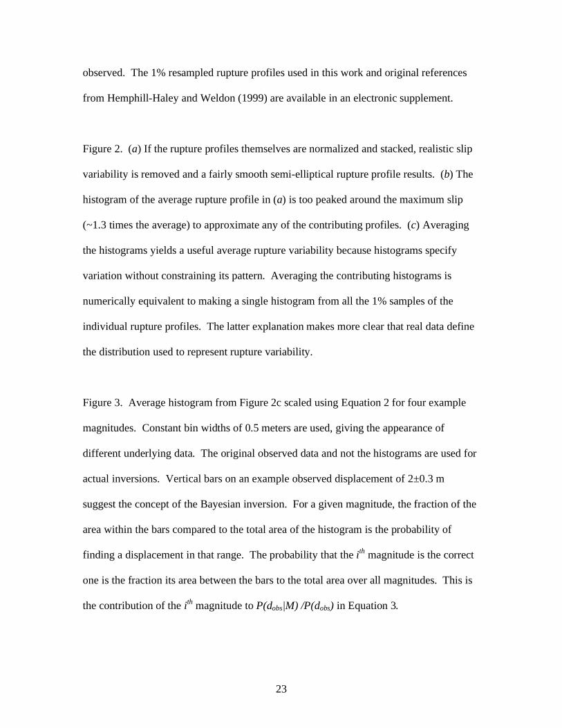
Figure 2. (a) If the rupture profiles themselves are normalized and stacked, realistic slip
variability is removed and a fairly smooth semi-elliptical rupture profile results. (b) The
histogram of the average rupture profile in (a) is too peaked around the maximum slip
(~1.3 times the average) to approximate any of the contributing profiles. (c) Averaging
the histograms yields a useful average rupture variability because histograms specify
variation without constraining its pattern. Averaging the contributing histograms is
numerically equivalent to making a single histogram from all the 1% samples of the
individual rupture profiles. The latter explanation makes more clear that real data define
the distribution used to represent rupture variability.
Figure 3. Average histogram from Figure 2c scaled using Equation 2 for four example
magnitudes. Constant bin widths of 0.5 meters are used, giving the appearance of
different underlying data. The original observed data and not the histograms are used for
actual inversions. Vertical bars on an example observed displacement of 2±0.3 m
suggest the concept of the Bayesian inversion. For a given magnitude, the fraction of the
area within the bars compared to the total area of the histogram is the probability of
finding a displacement in that range. The probability that the ith
magnitude is the correct
one is the fraction its area between the bars to the total area over all magnitudes. This is
the contribution of the ith magnitude to P(dobs|M) /P(dobs) in Equation 3.
24
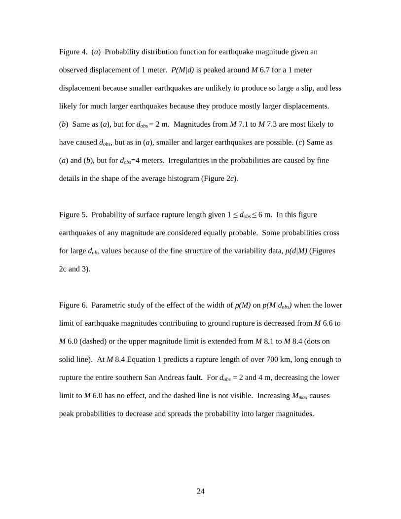
Figure 4. (a) Probability distribution function for earthquake magnitude given an
observed displacement of 1 meter. P(M|d) is peaked around M 6.7 for a 1 meter
displacement because smaller earthquakes are unlikely to produce so large a slip, and less
likely for much larger earthquakes because they produce mostly larger displacements.
(b) Same as (a), but for dobs = 2 m. Magnitudes from M 7.1 to M 7.3 are most likely to
have caused dobs, but as in (a), smaller and larger earthquakes are possible. (c) Same as
(a) and (b), but for dobs=4 meters. Irregularities in the probabilities are caused by fine
details in the shape of the average histogram (Figure 2c).
Figure 5. Probability of surface rupture length given 1 dobs 6 m. In this figure
earthquakes of any magnitude are considered equally probable. Some probabilities cross
for large dobs values because of the fine structure of the variability data, p(d|M) (Figures
2c and 3).
Figure 6. Parametric study of the effect of the width of p(M) on p(M|dobs) when the lower
limit of earthquake magnitudes contributing to ground rupture is decreased from M 6.6 to
M 6.0 (dashed) or the upper magnitude limit is extended from M 8.1 to M 8.4 (dots on
solid line). At M 8.4 Equation 1 predicts a rupture length of over 700 km, long enough to
rupture the entire southern San Andreas fault. For dobs = 2 and 4 m, decreasing the lower
limit to M 6.0 has no effect, and the dashed line is not visible. Increasing Mmax causes
peak probabilities to decrease and spreads the probability into larger magnitudes.
25
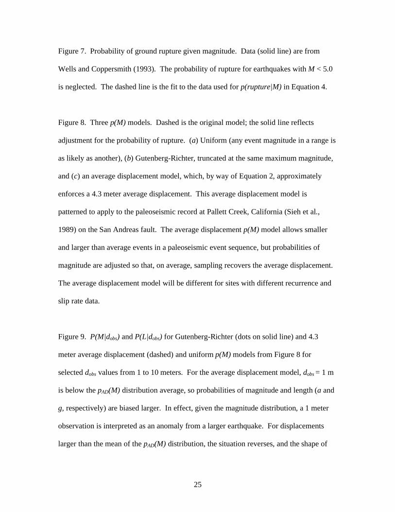
Figure 7. Probability of ground rupture given magnitude. Data (solid line) are from
Wells and Coppersmith (1993). The probability of rupture for earthquakes with M < 5.0
is neglected. The dashed line is the fit to the data used for p(rupture|M) in Equation 4.
Figure 8. Three p(M) models. Dashed is the original model; the solid line reflects
adjustment for the probability of rupture. (a) Uniform (any event magnitude in a range is
as likely as another), (b) Gutenberg-Richter, truncated at the same maximum magnitude,
and (c) an average displacement model, which, by way of Equation 2, approximately
enforces a 4.3 meter average displacement. This average displacement model is
patterned to apply to the paleoseismic record at Pallett Creek, California (Sieh et al.,
1989) on the San Andreas fault. The average displacement p(M) model allows smaller
and larger than average events in a paleoseismic event sequence, but probabilities of
magnitude are adjusted so that, on average, sampling recovers the average displacement.
The average displacement model will be different for sites with different recurrence and
slip rate data.
Figure 9. P(M|dobs) and P(L|dobs) for Gutenberg-Richter (dots on solid line) and 4.3
meter average displacement (dashed) and uniform p(M) models from Figure 8 for
selected dobs values from 1 to 10 meters. For the average displacement model, dobs = 1 m
is below the pAD(M) distribution average, so probabilities of magnitude and length (a and
g, respectively) are biased larger. In effect, given the magnitude distribution, a 1 meter
observation is interpreted as an anomaly from a larger earthquake. For displacements
larger than the mean of the pAD(M) distribution, the situation reverses, and the shape of

26
pAD(M) causes larger dobs to be interpreted as large outliers of a slightly smaller
magnitude and rupture length earthquake.
Acknowledgements
This work was supported by the National Earthquake Hazards Reduction Program,
Cooperative Agreements 1HQAG0009 and 4HQAG0004, and the Southern California
Earthquake Center. SCEC is funded by NSF Cooperative Agreement EAR-0106924 and
the USGS Cooperative Agreement 02HQAG0008. The SCEC contribution number for
this paper is 785.
27
References
Biasi, G.P., R. J. Weldon II, T. E. Fumal, and G. G. Seitz (2002). Paleoseismic event
dating and the conditional probability of large earthquakes on the southern San
Andreas fault, California, Bull. Seism. Soc. Am. 92, 2761-2781.
Bonilla, M. G. (1982). Evaluation of potential surface faulting and other tectonic
deformation, U.S. Geol. Surv. Open File Rept. 82-0732, 91 p.
Bonilla, M. G. (1988). Minimum earthquake magnitude associated with coseismic
surface faulting, Bull.Assoc. Eng. Geol., 25, 17-29.
Chang, W. L. and R. B. Smith (2002). Integrated seismic-hazard analysis of the Wasatch
Front, Utah, Bull. Seism. Soc. Am. 92, 1902-1922.
Fumal, T. E., Weldon, R. J., G. P. Biasi, T. E. Dawson, G. G. Seitz, W. T. Frost, and D.
P. Schwartz (2002a). Evidence for large earthquakes on the San Andreas fault at the
Wrightwood, California, paleoseismic site: A.D. 500 to Present, Bull. Seism. Soc.
Am. 92, 2726-2760.
Fumal, T. E., M. J. Rymer, and G. G. Seitz (2002b). Timing of large earthquakes since
A.D. 800 on the Mission Creek strand of the San Andreas fault zone at Thousand
Palms Oasis, near Palm Springs, California, Bull. Seism. Soc. Am. 92, 2841-2860.
Fumal, T.E., S. K. Pezzopane, R. J. Weldon II, and D. P. Schwartz (1993). A 100-year
average recurrence interval for the San Andreas fault at Wrightwood, California,
Science, 259, 199-203.
Grant, L. B. and K. Sieh (1994). Paleoseismic evidence of clustered earthquakes on the
San Andreas fault in the Carrizo Plain, California, J. Geophys. Res, 99, 6819-6841.
28
Hemphill-Haley, M. A. and R. J. Weldon II (1999). Estimating prehistoric earthquake
magnitude from point measurements of surface rupture, Bull. Seism. Soc. Am. 89,
1264-1279.
Lindvall, S. C., T. K. Rockwell, T. E. Dawson, J. G. Helms, and K. W. Bowman (2002).
Evidence for two surface ruptures in the past 500 years on the San Andreas fault at
Frazier Mountain, California, Bull. Seism. Soc. Am. 92, 2689-2703.
Liu, J., Y. Klinger, K. Sieh, and C. Rubin (2004). Six similar sequential ruptures of the San
Andreas fault, Carrizo Plain, California, Geology, 32, 649-652.
McCalpin, J. (1996). Paleoseismology, Academic Press, 588 pp.
McCalpin, J. and D. B. Slemmons (1998). Statistics of paleoseismic data, Final
Technical Report, Contract 1434-HQ-96-GR-02752, U.S.G.S. National Earthquake
Hazards Reduction Program, 62 pp.
Rockwell, T. K., J. Young, G. Seitz, A. Meltzner, D. Verdugo, F. Khatib, D. Ragona, O.
Altangerel, and J. West (2003). 3,000 years of ground-rupturing earthquakes in the
Anza Seismic Gap, San Jacinto fault, southern California: Time to shake it up?,
Seismol. Res. Lett., 74, 236.
Scholz, C. H. (2002). The Mechanics of Earthquakes and Faulting, Cambridge
University Press, Cambridge, 471 pp.
Schwartz, D. P. and K. J. Coppersmith (1984). Fault behavior and characteristic
earthquakes – Examples from the Wasatch and San Andreas fault zones, J. Geophys.
Res. 89, 5681-5698.
29
Salyards, S. L., K. E. Sieh, and J. L. Kirschvink (1992). Paleomagnetic measurement of
non-brittle coseismic deformation across the San Andreas fault at Pallett Creek, J.
Geophys. Res. 97, 12457-12470.
Seitz, G. G., R. J. Weldon II, and G. P. Biasi (1997). The Pitman Canyon paleoseismic
record: a re-evaluation of southern San Andreas fault segmentation, J. Geodynam.
24, 129-138.
Sieh, K. (1978). Slip along the San Andreas fault associated with the great 1857
earthquake, Bull. Seismol. Soc. Am. 68, 1421-1428.
Sieh, K. E. (1984). Lateral offsets and revised dates of large earthquakes at Pallett
Creek, California, J. Geophys. Res. 89, 7641-7670.
Sieh, K. E. (1986). Slip rate across the San Andreas fault and prehistoric earthquakes at
Indio, California, EOS Transactions, 67, 1200.
Sieh, K., M. Stuiver, and D. Brillinger (1989). A more precise chronology of
earthquakes produced by the San Andreas fault in southern California, J. Geophys.
Res., 94, 603-623.
Stirling, M., D. Rhoades, and K. Berryman (2002). Comparison of earthquake scaling
relations derived from data of the instrumental and pre-instrumental era, Bull. Seism.
Soc. Am., 92, 812-830.
Stirling, M. W., S. G. Wesnousky, and K. Shimazaki (1996). Fault trace complexity,
cumulative slip, and the shape of the magnitude-frequency distribution for strike-slip
faults: A global survey, Geophys. J. Int., 124, 833-868.
30
Weldon, R., K. Scharer, T. Fumal, and G. Biasi (2004). Wrightwood and the earthquake
cycle: what a long recurrence record tells us about how faults work, GSA Today, 14,
4-10.
Weldon, R. J. II, T. E. Fumal, T. J. Powers, S. K. Pezzopane, K. M. Scharer, and J. C.
Hamilton (2002). Structure and earthquake offsets on the San Andreas fault at the
Wrightwood, California paleoseismic site, Bull. Seism. Soc. Am. 92, 2704-2725.
Wells, D. L., and K. J. Coppersmith (1993). Likelihood of surface rupture as a function
of magnitude, Seismological Research Letters, 64, 54.
Wells, D. L., and K. J. Coppersmith (1994). New empirical relationships among
magnitude, rupture length, rupture width, rupture area, and surface displacement,
Bull. Seism. Soc. Am. 84, 974-1002.
Wesnousky, S. (1994). The Gutenberg-Richter or characteristic earthquake distribution,
which is it?, Bull. Seism. Soc. Am. 84, 1940-1959.
Yule, D. and C. Howland (2001). A revised chronology of earthquakes produced by the
San Andreas fault at Burro Flats, near Banning, California, in SCEC Annual Meeting,
Proceedings and Abstracts, Southern California Earthquake Center, Los Angeles,
121.
University of Nevada Reno
Seismological Laboratory, MS-174
Reno, NV 89557
(G.P.B.)

31
University of Oregon
Department of Geological Science 1272
Eugene, OR 97403
(R.J.W.)
0 0.5 10
0.5
1
1.5
2B olugerde
Normalized Length
No
rma
lize
d D
isp
lace
me
nt
0 2 40
0.1
0.2
D/Dave
0 0.5 10
1
2
3E dgecumbe
Normalized Length
No
rma
lize
d D
isp
lace
me
nt
0 2 40
0.2
0.4
D/Dave
0 0.5 10
1
2
3E rzincan
Normalized Length
No
rma
lize
d D
isp
lace
me
nt
0 2 40
0.2
0.4
D/Dave
0 0.5 10
0.5
1
1.5
2S an Andreas , 1857
Normalized Length
No
rma
lize
d D
isp
lace
me
nt
0 2 40
0.2
0.4
D/Dave
0 0.5 10
1
2
3F u� yun
Normalized Length
No
rma
lize
d D
isp
lace
me
nt
0 2 40
0.2
0.4
D/Dave
0 0.5 10
1
2
3K ern
Normalized Length
No
rma
lize
d D
isp
lace
me
nt
0 2 40
0.2
0.4
D/Dave
0 0.5 10
0.5
1
1.5
2T osya
Normalized Length
No
rma
lize
d D
isp
lace
me
nt
0 2 40
0.2
0.4
D/Dave
F igure 1
0 0.2 0.4 0.6 0.8 10
0.5
1
1.5
2
Normalized Length
D/D
ave
S tacked R upture P rofiles 1% S ampling
(a)
0 1 2 30
0.1
0.2
0.3
0.4
Normalized Displacement
Fre
qu
en
cy
His togram of S tacked R uptures
(b)
0 1 2 30
0.05
0.1
0.15
0.2
Normalized Displacement
Fre
qu
en
cy
His togram of All 1% d/dbar
F igure 2
(c)
0 5 100
0.2
0.4
0.6
Mw = 7.8
Displacement (m)
0 5 100
0.2
0.4
0.6
Mw = 7.4
0 5 100
0.2
0.4
0.6
Mw = 7
0 5 100
0.2
0.4
0.6
Mw = 6.6
Scaled Histograms of Displacement
Figure 3
6.5 7 7.5 8 8.50
0.05
0.1
0.15 dobs = 1.0 m
P (M|d) vs . Magnitude, dobs
1.00 to 4.00 m, prior: 1
Pro
ba
bili
ty
(a)
6.5 7 7.5 8 8.50
0.05
0.1
0.15 dobs = 2.0 m
Pro
ba
bili
ty
(b)
6.5 7 7.5 8 8.50
0.05
0.1
0.15 dobs = 4.0 m
Moment Magnitude
Pro
ba
bili
ty
(c)
F igure 4
0 100 200 300 400 5000
0.2
0.4
0.6
0.8
1
P (L|d) vs . R upture Length, dobs
1.00 to 6.00 m, prior: 1
S urface R upture Length (km)
Pro
ba
bili
ty
dobs
= 1
dobs
= 6
F igure 5
6 6.5 7 7.5 8 8.50
0.05
0.1
0.15 dobs = 1.0 m
p(M|d) for T hree Widths of Uniform p(M) P rior d
obs 1.00 to 4.00 m
Pro
ba
bili
ty (a)
6 6.5 7 7.5 8 8.50
0.05
0.1
0.15 dobs = 2.0 m
Pro
ba
bili
ty (b)
6 6.5 7 7.5 8 8.50
0.05
0.1
0.15 dobs = 4.0 m
Moment Magnitude
Pro
ba
bili
ty (c)
F igure 6
5 6 7 8 90
0.2
0.4
0.6
0.8
1F raction P roducing R upture, from W&C 1993
Magnitude
Fra
ctio
n
F igure 7
5 6 7 80
0.05
0.1
0.15
Pro
ba
bili
ty
Uniform P (M) Model
(a)
5 6 7 80
0.05
0.1
0.15
Pro
ba
bili
ty
G utenbergR ichter P (M) Model
(b)
5 6 7 80
0.05
0.1
0.15
Moment Mag
Pro
ba
bili
ty
C onstrained Mean Displacement P (M) Model
F igure 8
(c)
5 6 7 8 90
0.1
0.2
0.3 dobs = 1.0 m
p(M|d) vs. MagnitudePr
obab
ility
100 200 300 4000
0.5
1P(L|d) vs. Surface Rupture Length
dobs = 1.0 m
5 6 7 8 90
0.1
0.2
0.3 dobs = 2.0 m
Prob
abilit
y
100 200 300 4000
0.5
1dobs = 2.0 m
5 6 7 8 90
0.1
0.2
0.3 dobs = 4.0 m
Prob
abilit
y
100 200 300 400
0.20.40.60.8 dobs = 4.0 m
5 6 7 8 90
0.1
0.2
0.3 dobs = 6.0 m
Prob
abilit
y
100 200 300 4000
0.5
1dobs = 6.0 m
5 6 7 8 90
0.1
0.2
0.3 dobs = 8.0 m
Prob
abilit
y
100 200 300 4000
0.5
1dobs = 8.0 m
5 6 7 8 90
0.1
0.2
0.3 dobs = 10.0 m
Moment Magnitude
Prob
abilit
y
100 200 300 4000
0.5
1
Surface Rupture Length
dobs = 10.0 m
Figure 9
(a)
(b)
(c)
(d)
(e)
(f )
(g)
(h)
(i)
(j)
(k)
(l)
GRAD
Uniform