Estimating the Costs of Market Entry and Exit

for Video Rental Stores

Ying Fan∗

University of Michigan

June 1, 2016

Abstract

This paper uses information on entry and exit to estimate jointly video rental stores’ profits,

entry costs and sell-off values. I find that the distribution of sell-off values first-order stochas-

tically dominates that of entry costs, which suggests that the entry behavior in this industry

cannot be well captured by a static model because such a model implicitly assumes that a po-

tential entrant’s entry cost and an incumbent’s sell-off values are equal. I also find that the

entry decision seems to be a one-shot decision where the option value of waiting plays little role.

1 Introduction

Retail industries experience market entry and exit that is relatively frequent. This paper uses

information on entry and exit to jointly estimate retail stores’ profits, entry costs and sell-off

values. The idea is that stores enter into a market when they expect to be profitable, and stores

choose to exit when they expect the sell-off value to be higher than the value of continuing the

business. Entry and exit behavior therefore sheds light on the nature of profits, costs of entry,

and sell-off values. This paper makes two points. First, a static model does not capture the entry

and exit behavior well in the industry studied in this paper – video rental stores. Second, the

paper compares two alternative models of potential entrants’ entry decisions and concludes that

the model assuming that potential entrants are short-run players (i.e, they just make a decision

about whether to enter now or never) fits the data better.

Models of entry and exit have long been studied. Bresnahan and Reiss (1991) provide an entry

model with all competitors in the market being identical. Richer versions of the Brenahan and

∗Department of Economics, University of Michigan, 611 Tappan Street, Ann Arbor, MI 48109; yingfan@umich.edu.This paper is based on one chapter of my dissertation. I am indebted to my advisors Steve Berry, Hanming Fangand Philip Haile for their continual guidance, support and encouragement. I am also grateful to Patrick Bayer forhelp with the data.

1

Reiss model allow the competitors’ profits to be different. Berry (1992), for example, allows for

heterogeneity in both observed and unobserved costs. More recently, Seim (2006) and Mazzeo

(2002) add one more strategy dimension to study jointly the decisions about entry and quality

or location, respectively. All these models are either static or two-period models, and do not

distinguish entry and exit. They implicitly assume incumbents and potential entrants of a market

are identical in terms of facing the same opportunity costs (i.e., the costs of entry and sell-off values

are equal).

Dynamic models, on the other hand, relax these assumptions and explicitly use the information

on both entry and exit. This paper estimates a dynamic model of entry and exit in the video rental

industry. I find that the distribution of sell-off values of video rental stores first order stochastically

dominates the distribution of the cost of entry into the video rental market. This result is consistent

with the intuition that the one-period cost of entry is likely to be smaller than the sell-off values

that are related to the lifetime value of the stores. This result also indicates that the assumption

of equal entry cost and sell-off values in a static entry model does not hold.

Moreover, this paper investigates whether potential entrants in this industry are long-run or

short-run players. In a standard dynamic entry model, potential entrants are short-run players.

If they decide not to enter a market, they will never enter again. In other words, a potential

entrant either enters or perishes; and the value of waiting is zero. One exception is Fan and Xiao

(2015), which treats potential entrants as long-run players. In their model, the potential entrant,

in each period, compares the value of entry minus entry costs to the value of waiting when making

a decision about whether to enter or wait. In this paper, we consider both alternative models. By

estimating both models and comparing their fit to the data, I find that video rental stores’ entry

decision seems to be a one-shot decision. This is in contrast to Fan and Xiao (2015), which finds

that local telephone firms are long-run players. One explanation for this difference in the findings is

that video rental stores are generally smaller than local telephone firms, and the entry cost is also

likely to be smaller. As a result, the video rental stores are more likely to make a simple decision

on entry or not, rather than on the timing of entry.

The empirical context of this paper is video rental stores. Even though the video rental in-

dustry is declining, the following characteristics of this industry make the model described below

particularly suitable: the products in this industry are relatively homogenous, and this industry

experiences relatively frequent entry and exit, which helps identification.

By highlighting the importance of considering the dynamic behavior in an entry model and com-

paring two alternative dynamic entry model, this paper contributes to the literature on dynamic

entry game estimation. Examples in this literature include Victor Aguirregabiria (2007), Bajari,

Benkard and Levin (2007), Pakes, Ostrovsky and Berry (2007) and Pesendorfer and Schmidt-

Dengler (2008).1 The computation of a dynamic oligopoly model is quite burdensome. The straight-

1Other examples include Ryan (2012), Collard-Wexler (2013) and Dunne, Klimek, Roberts and Xu (2013).

2

forward way would be to compute the equilibrium strategies for any given set of parameters, and

search for the parameters to make the implications of the equilibrium strategies as close to the

data as possible. To compute the equilibrium strategies of a dynamic game, however, one needs

to know the value functions, which are in turn determined by the strategies played. Furthermore,

the evolution of the markets is endogenous. Thus, computing a dynamic oligopoly model with a

realistic number of competitors is prohibitive. This paper follows the estimation strategy provided

by Pakes, Ostrovsky and Berry (2007) (henceforth, POB) to avoid this computation, and estimate

the value functions directly for any given parameters.2 But different from POB which relies on

simulated data, this paper uses actual industry data and has to deal with – and thus provides

solutions to – several practical issues.

The rest of the paper is organized as follows. Section 2 develops the dynamic entry and exit

model. Section 3 describes the estimation procedure. The data are described in Section 4. The

empirical results are presented in section 5. Section 6 concludes the paper.

2 Model

This section presents a dynamic model of entry and exit. The model presented here largely follows

the one in POB. Let nt be the number of video rental stores in the market at the beginning of

year t, and mt the market size that evolves exogenously according to a first-order Markov chain.3 I

assume stores in the market have the same profit function and the profits are determined solely by

the number of incumbents and the market size. Furthermore, I assume that the one-period profit

function has the following parametric form:

π (n,m; η, θ) =mη

(1 + n)θ,

where η and θ are parameters to be estimated.

2.1 An Incumbent’s Decision

In each period, each incumbent j observes its sell-off value of the video rental store, denoted by φjt,

which is incumbent j’s private information. Assume that φjt is i.i.d. across j and t, and follows

an exponential distribution with expectation σ. With the knowledge of φjt, incumbent j has two

choices: staying in business or exiting. I assume that upon exit, the store will not go back to

business again. Let V I (n,m, φ; η, θ) be the value of an incumbent with sell-off value φ at state

2Jofre-Bonet and Pesendorfer (2003) is another paper that uses the this idea to estimate the value function.3In the empirical implementation, I will measure market size by population size.

3

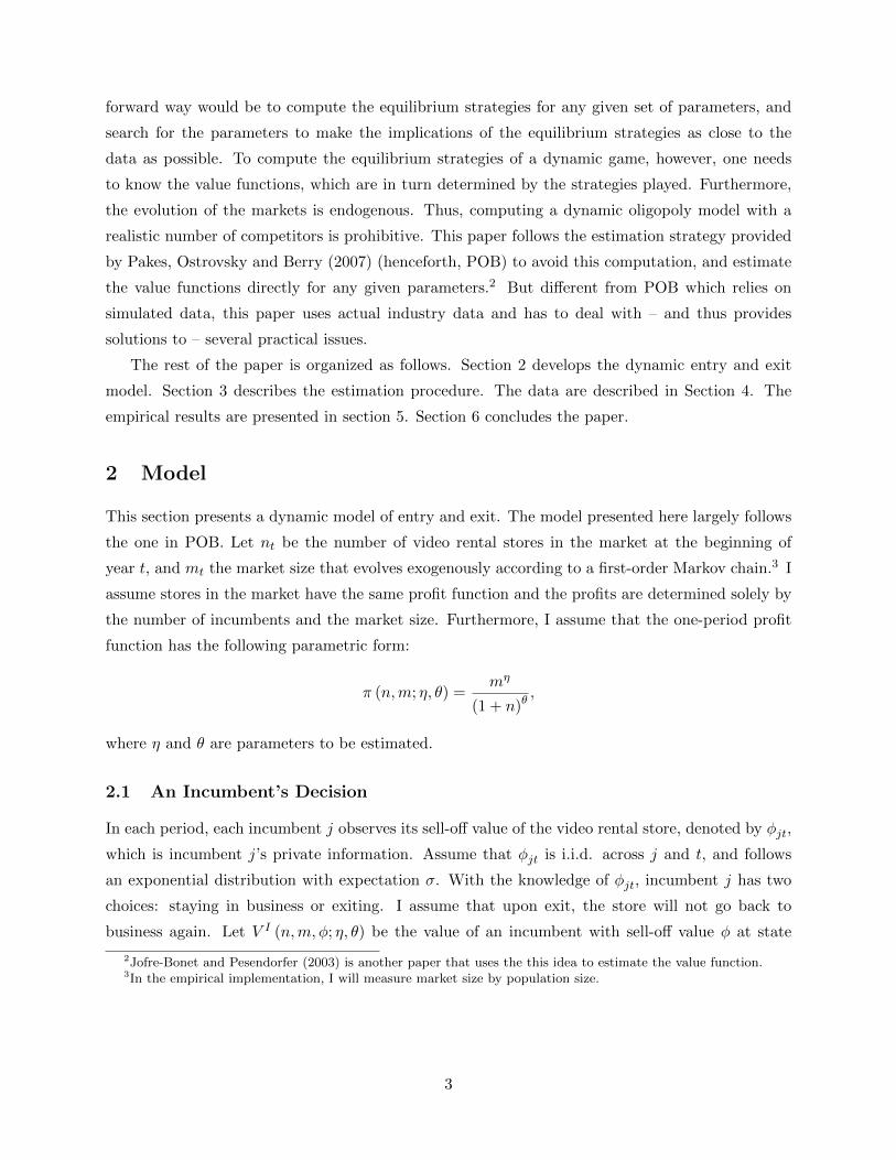
(n,m). Then, the Bellman equation for a typical incumbent problem is

V I (n,m, φ; η, θ) = π (n,m; η, θ) + βmax{Ec(n′,m′)|(n,m)Eφ′V

I(n′,m′, φ′; η, θ

), φ}, (1)

where(n′,m′, φ′

)denotes, respectively, the number of stores, the market size and the sell-off value

next period. The expectation operator Ec(n′,m′)|(n,m) denotes the incumbent’s expectation of (n′,m′)

conditional on itself continuing at state (n,m), and Eφ′ is the expectation over φ′. The stores

discount future profit at discount rate β. The problem for incumbents is summarized by Figure 1.

Figure 1: Incumbent’s problem

Incumbent

[ , ,IV n m ]

exit [ ,n m ]

stay [ ,n m ]

this period next period expectation operator

Incumbent

[ ', ', 'IV n m ]

Outsider

[ ]

'', ' |( , )

c

n m n mE E

2.2 A Potential Entrant’s Decision

I now turn to a potential entrant’s entry decision. I assume that there are ε potential entrants

in each market, which is common knowledge among potential entrants and incumbents. Potential

entrant j observes the cost of entry ϕjt at the beginning of period t. Like the sell-off value φjt, the

entry cost ϕjt is also assumed to be private information to j, and identically and independently

distributed across potential entrants and time. If j decides to enter the market, it has to pay the

cost of entry ϕjt to set up the business, and starts earning profits next period. Therefore, the value

of entry is the expected value of being an incumbent next period. The potential entrant’s decision

is based on the comparison of this value of entry net of entry cost with the value of waiting. I now

describe two alternative models to capture a potential entrant’s decision.

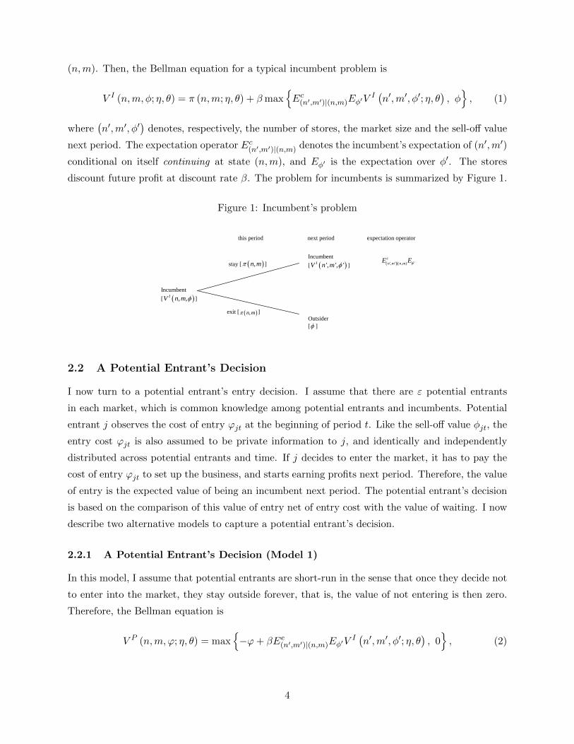
2.2.1 A Potential Entrant’s Decision (Model 1)

In this model, I assume that potential entrants are short-run in the sense that once they decide not

to enter into the market, they stay outside forever, that is, the value of not entering is then zero.

Therefore, the Bellman equation is

V P (n,m,ϕ; η, θ) = max{−ϕ+ βEe(n′,m′)|(n,m)Eφ′V

I(n′,m′, φ′; η, θ

), 0}, (2)

4

where V P (n,m,ϕ; η, θ) is the value of a potential entrant, and Ee(n′,m′)|(n,m) is the potential entrant’s

expectation of (n′,m′) conditional on itself entering at state (n,m).

In this model, I assume that the density of the distribution of entry fees is given by

f (z) = λ2(z − 1

λ

)exp

[−λ(z − 1

λ

)](3)

for z ≥ 1λ . This is a gamma distribution with one parameter fixed at 2. Here, 1

λ is the boundary of

the support for the entry cost ϕ.4 This implies that the value of entry has to be high enough for

there to be any entry. This model of potential entrants can be summarized by Figure 2.

Figure 2: Potential Entrant’s Problem (Model 1: Short-run Player)

Not enter [0]

Enter [ ]

this period next period expectation operator

Incumbent

[ ', ', 'IV n m ]

Outsider

[0]

Potential Entrant

[ , ,EV n m ]

'', ' |( , )

e

n m n mE E

2.2.2 A Potential Entrant’s Decision (Model 2)

Alternatively, if the potential entrants are long-run players and the timing of entry is a consideration,

the value of waiting is the expected value of being a potential entrant next period, and the Bellman

equation becomes

V P (n,m,ϕ; η, θ) = max{−ϕ+ βEe(n′,m′)|(n,m)Eφ′V

I(n′,m′, φ′; η, θ

), (4)

βEw(n′,m′)|(n,m)Eϕ′VP(n′,m′, ϕ′; η, θ

)},

where Ew(n′,m′) is the potential entrant’s expectation conditional on itself waiting. Note the difference

of the value functions and the expectation operators in the first term and the second term in (4).

Since the value of waiting for a long-run player is the expected value of being a potential entrant

next period, the expectation is taken over the distribution of next period’s entry cost ϕ′ and over

the state next period (n′,m′) conditional on itself waiting.

In Model 1, I impose a lower bound on the entry cost so that the value of entry needs to be

high enough for there to be any entry. In Model 2, because the value of waiting is no longer zero,

I do not need to impose such a lower bound anymore. In other words, the density function of the

4Following POB, I assume the lower bound of the support is 1λ

, instead of introducing an additional parameter.

5

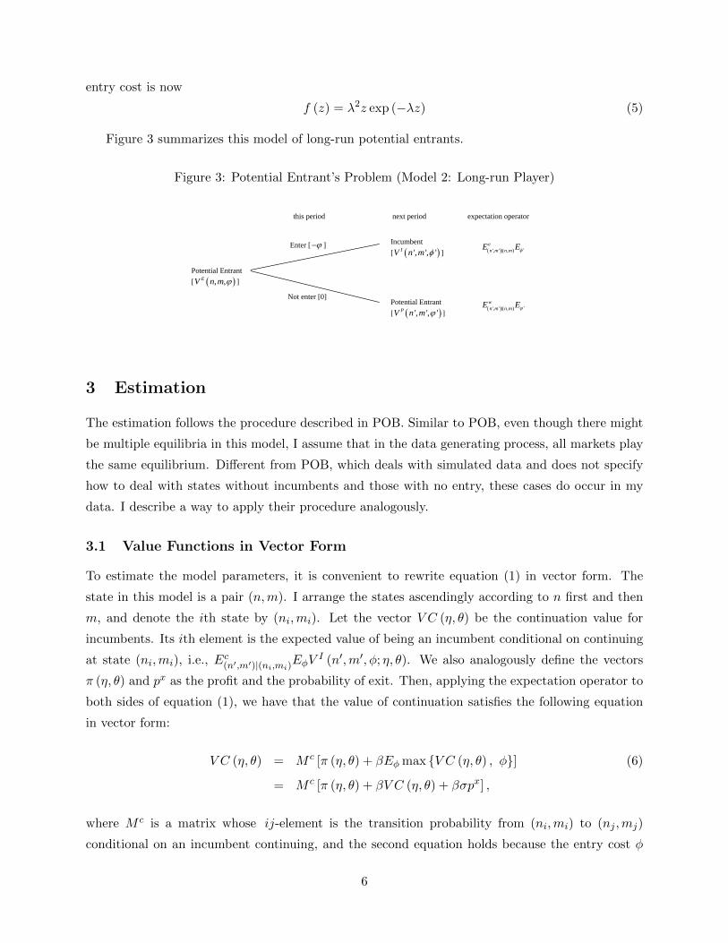
entry cost is now

f (z) = λ2z exp (−λz) (5)

Figure 3 summarizes this model of long-run potential entrants.

Figure 3: Potential Entrant’s Problem (Model 2: Long-run Player)

Not enter [0]

Enter [ ]

this period next period expectation operator

Incumbent

[ ', ', 'IV n m ]

Potential Entrant

[ ', ', 'PV n m ]

Potential Entrant

[ , ,EV n m ]

'', ' |( , )

w

n m n mE E

'', ' |( , )

e

n m n mE E

3 Estimation

The estimation follows the procedure described in POB. Similar to POB, even though there might

be multiple equilibria in this model, I assume that in the data generating process, all markets play

the same equilibrium. Different from POB, which deals with simulated data and does not specify

how to deal with states without incumbents and those with no entry, these cases do occur in my

data. I describe a way to apply their procedure analogously.

3.1 Value Functions in Vector Form

To estimate the model parameters, it is convenient to rewrite equation (1) in vector form. The

state in this model is a pair (n,m). I arrange the states ascendingly according to n first and then

m, and denote the ith state by (ni,mi). Let the vector V C (η, θ) be the continuation value for

incumbents. Its ith element is the expected value of being an incumbent conditional on continuing

at state (ni,mi), i.e., Ec(n′,m′)|(ni,mi)EφVI (n′,m′, φ; η, θ). We also analogously define the vectors

π (η, θ) and px as the profit and the probability of exit. Then, applying the expectation operator to

both sides of equation (1), we have that the value of continuation satisfies the following equation

in vector form:

V C (η, θ) = M c [π (η, θ) + βEφ max {V C (η, θ) , φ}] (6)

= M c [π (η, θ) + βV C (η, θ) + βσpx] ,

where M c is a matrix whose ij-element is the transition probability from (ni,mi) to (nj ,mj)

conditional on an incumbent continuing, and the second equation holds because the entry cost φ

6

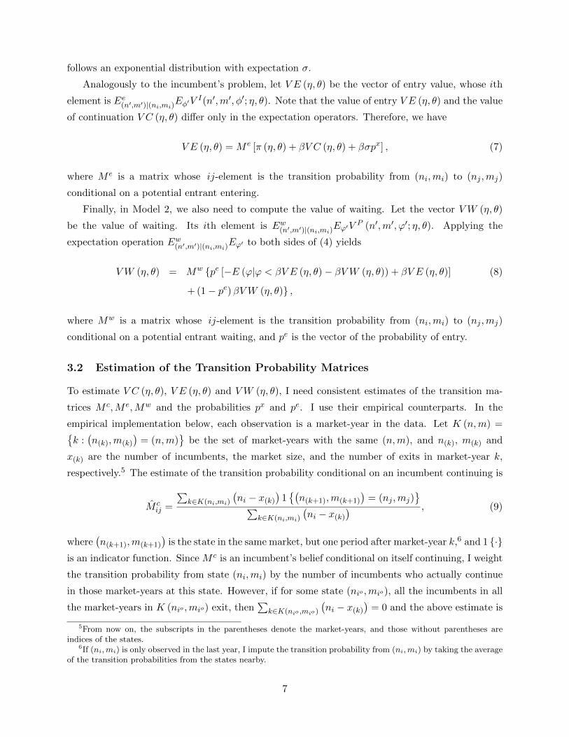
follows an exponential distribution with expectation σ.

Analogously to the incumbent’s problem, let V E (η, θ) be the vector of entry value, whose ith

element is Ee(n′,m′)|(ni,mi)Eφ′VI(n′,m′, φ′; η, θ). Note that the value of entry V E (η, θ) and the value

of continuation V C (η, θ) differ only in the expectation operators. Therefore, we have

V E (η, θ) = M e [π (η, θ) + βV C (η, θ) + βσpx] , (7)

where M e is a matrix whose ij-element is the transition probability from (ni,mi) to (nj ,mj)

conditional on a potential entrant entering.

Finally, in Model 2, we also need to compute the value of waiting. Let the vector VW (η, θ)

be the value of waiting. Its ith element is Ew(n′,m′)|(ni,mi)Eϕ′VP (n′,m′, ϕ′; η, θ). Applying the

expectation operation Ew(n′,m′)|(ni,mi)Eϕ′ to both sides of (4) yields

VW (η, θ) = Mw {pe [−E (ϕ|ϕ < βV E (η, θ)− βVW (η, θ)) + βV E (η, θ)] (8)

+ (1− pe)βVW (η, θ)} ,

where Mw is a matrix whose ij-element is the transition probability from (ni,mi) to (nj ,mj)

conditional on a potential entrant waiting, and pe is the vector of the probability of entry.

3.2 Estimation of the Transition Probability Matrices

To estimate V C (η, θ), V E (η, θ) and VW (η, θ), I need consistent estimates of the transition ma-

trices M c,M e,Mw and the probabilities px and pe. I use their empirical counterparts. In the

empirical implementation below, each observation is a market-year in the data. Let K (n,m) ={k :(n(k),m(k)

)= (n,m)

}be the set of market-years with the same (n,m), and n(k), m(k) and

x(k) are the number of incumbents, the market size, and the number of exits in market-year k,

respectively.5 The estimate of the transition probability conditional on an incumbent continuing is

M cij =

∑k∈K(ni,mi)

(ni − x(k)

)1{(n(k+1),m(k+1)

)= (nj ,mj)

}∑k∈K(ni,mi)

(ni − x(k)

) , (9)

where(n(k+1),m(k+1)

)is the state in the same market, but one period after market-year k,6 and 1 {·}

is an indicator function. Since M c is an incumbent’s belief conditional on itself continuing, I weight

the transition probability from state (ni,mi) by the number of incumbents who actually continue

in those market-years at this state. However, if for some state (nio ,mio), all the incumbents in all

the market-years in K (nio ,mio) exit, then∑

k∈K(nio ,mio )

(ni − x(k)

)= 0 and the above estimate is

5From now on, the subscripts in the parentheses denote the market-years, and those without parentheses areindices of the states.

6If (ni,mi) is only observed in the last year, I impute the transition probability from (ni,mi) by taking the averageof the transition probabilities from the states nearby.

7

not valid. In this case, the estimate is

M cioj =

∑k∈K(nio ,mio )

1{e(k) = nj − 1,m(k+1) = mj

}#K (nio ,mio)

, (10)

where e(k) is the number of entrants in market-year k. Since the estimate of the probability of exit

at (nio ,mio) is 1 in this case, the incumbent believes that all other incumbents will exit. Conditional

on itself continuing, the probability of transiting to state (nj ,mj) equals the probability of e = nj−1

and m′ = mj .7

Similarly, the estimate of a potential entrant’s belief about the state next period conditional on

itself entering is

M eij =

∑k∈K(ni,mi)

e(k)1{(n(k+1),m(k+1)

)= (nj ,mj)

}∑k∈K(ni,mi)

e(k). (11)

I weight the transition probability by the number of potential entrants who actually enter.

If at some state (nio ,mio) , no store enters in any market-year in K (nio ,mio), then the estimate

is

M eioj =

∑k∈K(nio ,mio )

1{x(k) = nio + 1− nj ,m(k+1) = mj

}#K (nio ,mio)

. (12)

The idea is similar to the one leading to (10): when the entrant expects itself to be the only one

entering, the probability of transiting from state (nio ,mio) to state (nj ,mj) conditional on itself

entering equals the probability of nio − x+ 1 = nj and m′ = mj .8

Finally, the estimate of the transition probabilities conditional on waiting Mw is given by

Mwij =

∑k∈K(ni,mi)

(ε− e(k)

)1{(n(k+1),m(k+1)

)= (nj ,mj)

}∑k∈K(ni,mi)

(ε− e(k)

) . (13)

The weight used here is the number of potential entrants who did not enter.

As for the exit probability and the entry probability at state (n,m), their estimates are, respec-

tively,

px (n,m) =1

#K (n,m)

∑k∈K(n,m)

x(k)

n, (14)

7Another way to obtain this is to explicitly write down the conditional transition probability. The probability oftransiting from state (ni,mi) to state (nj ,mj) is

∑(e,x) s.t. nj=ni+e−x

bx (x, ni − 1|ni,mi) be (e, ε|ni,mi) Pr (mj |mi),

where bx (x, ni − 1|ni,mi) is the probability of x out of (ni − 1) incumbents exiting at state (ni,mi), andbe (e, ε|ni,mi) is the probability of e out of ε potential entrants entering at state (ni,mi). When the probabilityof exit is 1 at state (nio ,mio), bx (x, nio − 1|nio ,mio) = 0 for x < nio − 1 and = 1 for x = nio − 1. So, the transitionprobability is reduced to be (nj − 1, ε|nio ,mio) Pr (mj |mio). And the empirical counterpart of it is exactly the RHSof equation (10).

8Again, this expression can be obtained mathematically by noting that this conditional probability of transiting is∑(e,x) s.t. nj=ni+e−x

bx (x, ni|ni,mi) be (e− 1, ε− 1|ni,mi) Pr (mj |mi) = bx (ni + 1− nj , ε|ni,mi) Pr (mj |mi) when the

probability of entering is zero.

8

and

pe (n,m) =1

#K (n,m)

∑k∈K(n,m)

e(k)

ε. (15)

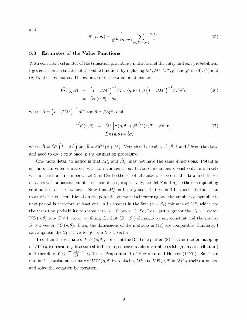
3.3 Estimates of the Value Functions

With consistent estimates of the transition probability matrices and the entry and exit probabilities,

I get consistent estimates of the value functions by replacing M c,M e,Mw, px and pe in (6), (7) and

(8) by their estimates. The estimates of the value functions are

V C (η, θ) =(I − βM c

)−1M cπ (η, θ) + β

(I − βM c

)−1M cpxσ (16)

= Aπ (η, θ) + aσ,

where A =(I − βM c

)−1M c and a = βApx, and

V E (η, θ) = M e[π (η, θ) + βV C (η, θ) + βpxσ

](17)

= Bπ (η, θ) + bσ,

where B = M e(I + βA

)and b = βM e (a+ px). Note that I calculate A, B, a and b from the data,

and need to do it only once in the estimation procedure.

One more detail to notice is that M eij and M c

ij may not have the same dimensions. Potential

entrants can enter a market with no incumbent, but trivially, incumbents exist only in markets

with at least one incumbent. Let S and S1 be the set of all states observed in the data and the set

of states with a positive number of incumbents, respectively, and let S and S1 be the corresponding

cardinalities of the two sets. Note that M eij = 0 for j such that nj = 0 because this transition

matrix is the one conditional on the potential entrant itself entering and the number of incumbents

next period is therefore at least one. All elements in the first (S − S1) columns of M e, which are

the transition probability to states with n = 0, are all 0. So, I can just augment the S1 × 1 vector

V C (η, θ) to a S × 1 vector by filling the first (S − S1) elements by any constant and the rest by

S1 × 1 vector V C (η, θ). Then, the dimensions of the matrices in (17) are compatible. Similarly, I

can augment the S1 × 1 vector px to a S × 1 vector.

To obtain the estimate of VW (η, θ), note that the RHS of equation (8) is a contraction mapping

of VW (η, θ) because ϕ is assumed to be a log concave random variable (with gamma distribution)

and therefore, 0 ≤ ∂E(ϕ|ϕ<d)∂d ≤ 1 (see Proposition 1 of Heckman and Honore (1990)). So, I can

obtain the consistent estimate of VW (η, θ) by replacing Mw and V E (η, θ) in (8) by their estimates,

and solve the equation by iteration.

9

3.4 Moment Conditions

I estimate four parameters – profit function parameters (η, θ) and distribution parameters (σ, λ) –

using four moment conditions. The first two conditions make the model predictions of the entry

and exit probabilities as close as possible to the frequencies observed in the data as possible. The

third and fourth conditions posit that prediction errors are uncorrelated with market sizes.

Specifically, let the prediction error of entry and exit at state (n,m) be

Xerror (n,m) = px (n,m; η, θ, σ) · n− 1

#K (n,m)

(∑k∈K(n,m)

x(k)

),

Eerror (n,m) = pe (n,m; η, θ, λ) · ε− 1

#K (n,m)

(∑k∈K(n,m)

e(k)

),

where the model prediction of the exit probability px (n,m; η, θ, λ) = Pr(φ ≥ V C (η, θ) ;σ

), and

the model prediction of the entry probability pe (n,m; η, θ, λ) is Pr(ϕ ≤ βV E (η, θ) ;λ

)in Model

1 and Pr(ϕ ≤ βV E (η, θ)− βV W (η, θ) ;λ

)in Model 2.

Using the denotations Xerror (n,m) and Eerror (n,m), the empirical counterparts of the four

moments can be written as1

S

∑(n,m)∈S

Eerror (n,m) = 0 (18)

1

S1

∑(n,m)∈S1

Xerror (n,m) = 0 (19)

1

#M

∑m∈M

1

#N (m)

∑ni∈N(m)

Eerror (ni,m)

·m = 0 (20)

1

#M

∑m∈M

1

#N1 (m)

∑ni∈N1(m)

Xerror (ni,m)

·m = 0 (21)

where N (m) = {n : (n,m) ∈ S} is the set of incumbent numbers that are observed in the data for a

given m, N1 (m) = {n : (n,m) ∈ S1} is the set of positive numbers of incumbents that are observed

in the data for given m, and M = {m : (n,m) ∈ S} is the set of market sizes observed in the data.

4 Data

The data for the number of incumbents, entrants and exits are taken from the National Establish-

ment Time-Series Database (California). This data is designed to describe the dynamics of the U.S.

economy. It keeps track of the birth, death and relocation of all the establishments that were ever in

business in California between 1990 and 2004. This dataset is therefore ideal for studying the issue

10

of entry and exit.9 Population data in 1990 and 2000 come from the decennial census. Population

data in the years between 1991 and 1999 is from the estimates provided by the Population Division

of Department of Finance in California. Population after 2000 comes from the estimates from the

Population Division of U.S. Census Bureau.

The National Establishment Time-Series Database has data for the years between 1990 and

2004. But since I do not have complete information about exits in the last year, the sample I use

for estimation is between 1990 and 2003. More specifically, the sample is constructed as follows.

Markets in this paper are Census places. I choose this definition of market mainly because

of data availability. For years without a census, the smallest geographic unit with population

estimates is Census place. There are 428 places in California with population data in all the years

between 1990 and 2003 and having video rental stores in at least one of the years. However, cities

as large as Los Angels and San Diego obviously cannot be considered as just one market for the

video renting industry. Due to the high transportation cost relative to the price of renting videos,

video rental stores at either end of the large cities would rarely be in a direct competition with

each other. According to an annual report of the Video Software Dealers Association, the average

customer travels only 3.2 miles in total for a round trip to a video rental store. With this concern,

I restrict the markets in this study to be places with a population smaller than 150,000 and leave

out 29 places with a population larger than that. Furthermore, I leave out 8 cities which have a

number of video rental stores larger than 20 in at least one of the years. Including these 8 cities in

the sample would increase the number of possible states the state variables can obtain by 23, and

13 of them have been observed only once in the data. I leave them out in order to reduce sampling

error. So, the data used in this study is panel data with 391 markets in 14 years.

The number of incumbents in market c at time t is the number of establishments with the first

four digits of the Primary Standard Industrial Classification (SIC) code at time t equal to “7841”,

which is the SIC code for “Video Tape Rental” industry. Number of entrants in market c at time t

is the sum of the followings three: (i) the number of establishments that started business as video

stores in market c at time t; (ii) the number of establishments that switched from other business

to video rental store at time t, and was in market c at time t; (iii) the number of establishments

that moved from other places to market c at time t and were video rental stores after moving, no

matter whether they were video stores before moving. Similarly, an establishment is considered as

an exitor in market c at time t if it falls into one of the following three categories: (i) video stores

in market c whose last year in business was t; (ii) video stores in market c that switched to another

business at time t (the first four digits of the SIC code in year t are 7841 and those in year t + 1

9One caveat of the dataset is that it does not provide information on whether a store is a company-owned chainstore, which may be different from other stores in terms of profitability or entry costs. During the sample periodof 1990 – 2004, there were two main video rental chains, Blockbuster and Hollywood Video. Their stores, includingboth the franchised ones and the company-owned ones, account for about 7% of all video rental stores ever in thesample, implying that “independent” stores do play an important role in this industry.

11

are not); (iii) video stores in market c that moved out of the market, no matter whether they were

video stores after moving.

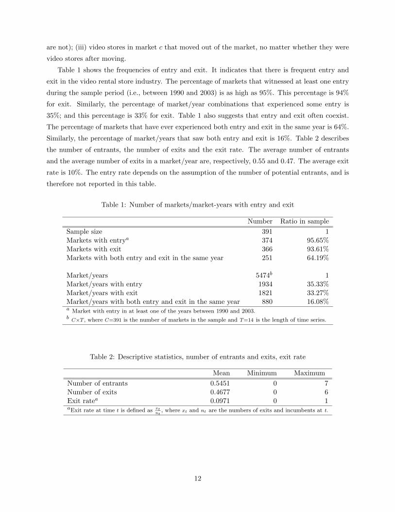
Table 1 shows the frequencies of entry and exit. It indicates that there is frequent entry and

exit in the video rental store industry. The percentage of markets that witnessed at least one entry

during the sample period (i.e., between 1990 and 2003) is as high as 95%. This percentage is 94%

for exit. Similarly, the percentage of market/year combinations that experienced some entry is

35%; and this percentage is 33% for exit. Table 1 also suggests that entry and exit often coexist.

The percentage of markets that have ever experienced both entry and exit in the same year is 64%.

Similarly, the percentage of market/years that saw both entry and exit is 16%. Table 2 describes

the number of entrants, the number of exits and the exit rate. The average number of entrants

and the average number of exits in a market/year are, respectively, 0.55 and 0.47. The average exit

rate is 10%. The entry rate depends on the assumption of the number of potential entrants, and is

therefore not reported in this table.

Table 1: Number of markets/market-years with entry and exit

Number Ratio in sample

Sample size 391 1Markets with entrya 374 95.65%Markets with exit 366 93.61%Markets with both entry and exit in the same year 251 64.19%

Market/years 5474b 1Market/years with entry 1934 35.33%Market/years with exit 1821 33.27%Market/years with both entry and exit in the same year 880 16.08%a Market with entry in at least one of the years between 1990 and 2003.b C×T , where C=391 is the number of markets in the sample and T=14 is the length of time series.

Table 2: Descriptive statistics, number of entrants and exits, exit rate

Mean Minimum Maximum

Number of entrants 0.5451 0 7Number of exits 0.4677 0 6Exit ratea 0.0971 0 1aExit rate at time t is defined as xt

nt, where xt and nt are the numbers of exits and incumbents at t.

12

5 Empirical results

The discount rate used in the estimation is given by 0.8, following Jofre-Bonet and Pesendorfer

(2003). A state in this study is a pair (n,m), where n is the number of incumbents and m is the

market size. The number of incumbents, n, varies from 0 to 20 in the sample. I discretize population

by dividing the population data into a grid of 40 bins with the same number of observations in

each bin and use the median of each bin as m.10 Standard deviations of the estimates are obtained

by bootstrap.

Table 3 presents the estimation results based on Model 1 where a potential entrant is a short-

run player. The four columns show the estimation results for the model with different numbers of

potential entrants, which varies from 7 to 10. Table 3 indicates that the results are robust to the

number of potential entrants. In what follows, I focus on the results with 7 potential entrants.

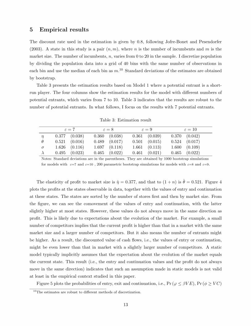
Table 3: Estimation result

ε = 7 ε = 8 ε = 9 ε = 10

η 0.377 (0.038) 0.360 (0.038) 0.361 (0.039) 0.370 (0.042)θ 0.521 (0.016) 0.489 (0.017) 0.501 (0.015) 0.524 (0.017)σ 1.626 (0.116) 1.697 (0.118) 1.661 (0.113) 1.600 (0.109)λ 0.495 (0.023) 0.465 (0.022) 0.461 (0.021) 0.465 (0.022)

Notes: Standard deviations are in the parentheses. They are obtained by 1000 bootstrap simulations

for models with ε=7 and ε=10 , 200 parametric bootstrap simulations for models with ε=8 and ε=9.

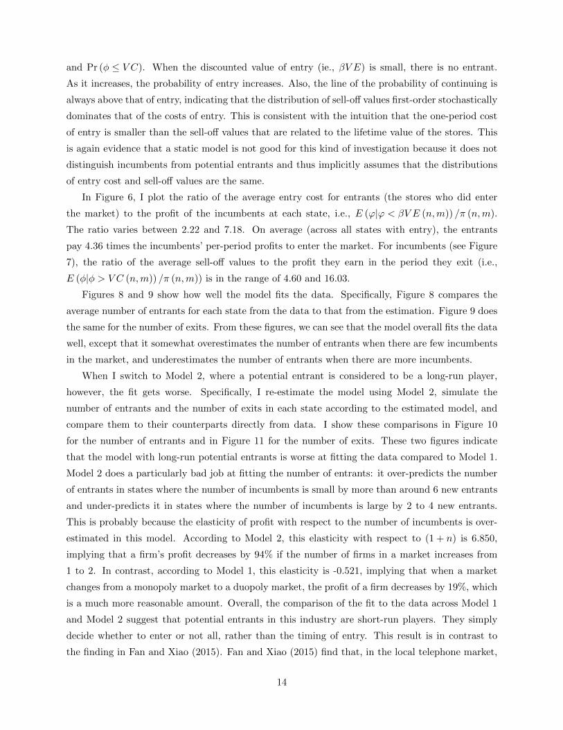
The elasticity of profit to market size is η = 0.377, and that to (1 + n) is θ = 0.521. Figure 4

plots the profits at the states observable in data, together with the values of entry and continuation

at these states. The states are sorted by the number of stores first and then by market size. From

the figure, we can see the comovement of the values of entry and continuation, with the latter

slightly higher at most states. However, these values do not always move in the same direction as

profit. This is likely due to expectations about the evolution of the market. For example, a small

number of competitors implies that the current profit is higher than that in a market with the same

market size and a larger number of competitors. But it also means the number of entrants might

be higher. As a result, the discounted value of cash flows, i.e., the values of entry or continuation,

might be even lower than that in market with a slightly larger number of competitors. A static

model typically implicitly assumes that the expectation about the evolution of the market equals

the current state. This result (i.e., the entry and continuation values and the profit do not always

move in the same direction) indicates that such an assumption made in static models is not valid

at least in the empirical context studied in this paper.

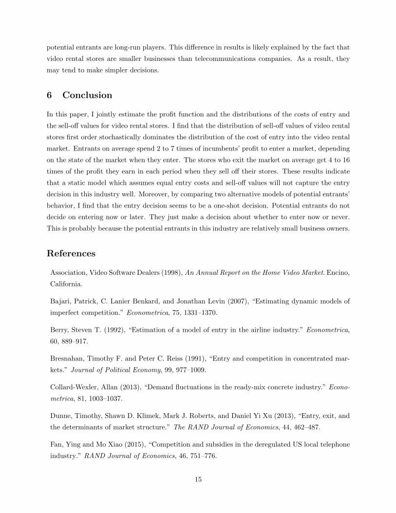
Figure 5 plots the probabilities of entry, exit and continuation, i.e., Pr (ϕ ≤ βV E), Pr (φ ≥ V C)

10The estimates are robust to different methods of discretization.

13

and Pr (φ ≤ V C). When the discounted value of entry (ie., βV E) is small, there is no entrant.

As it increases, the probability of entry increases. Also, the line of the probability of continuing is

always above that of entry, indicating that the distribution of sell-off values first-order stochastically

dominates that of the costs of entry. This is consistent with the intuition that the one-period cost

of entry is smaller than the sell-off values that are related to the lifetime value of the stores. This

is again evidence that a static model is not good for this kind of investigation because it does not

distinguish incumbents from potential entrants and thus implicitly assumes that the distributions

of entry cost and sell-off values are the same.

In Figure 6, I plot the ratio of the average entry cost for entrants (the stores who did enter

the market) to the profit of the incumbents at each state, i.e., E (ϕ|ϕ < βV E (n,m)) /π (n,m).

The ratio varies between 2.22 and 7.18. On average (across all states with entry), the entrants

pay 4.36 times the incumbents’ per-period profits to enter the market. For incumbents (see Figure

7), the ratio of the average sell-off values to the profit they earn in the period they exit (i.e.,

E (φ|φ > V C (n,m)) /π (n,m)) is in the range of 4.60 and 16.03.

Figures 8 and 9 show how well the model fits the data. Specifically, Figure 8 compares the

average number of entrants for each state from the data to that from the estimation. Figure 9 does

the same for the number of exits. From these figures, we can see that the model overall fits the data

well, except that it somewhat overestimates the number of entrants when there are few incumbents

in the market, and underestimates the number of entrants when there are more incumbents.

When I switch to Model 2, where a potential entrant is considered to be a long-run player,

however, the fit gets worse. Specifically, I re-estimate the model using Model 2, simulate the

number of entrants and the number of exits in each state according to the estimated model, and

compare them to their counterparts directly from data. I show these comparisons in Figure 10

for the number of entrants and in Figure 11 for the number of exits. These two figures indicate

that the model with long-run potential entrants is worse at fitting the data compared to Model 1.

Model 2 does a particularly bad job at fitting the number of entrants: it over-predicts the number

of entrants in states where the number of incumbents is small by more than around 6 new entrants

and under-predicts it in states where the number of incumbents is large by 2 to 4 new entrants.

This is probably because the elasticity of profit with respect to the number of incumbents is over-

estimated in this model. According to Model 2, this elasticity with respect to (1 + n) is 6.850,

implying that a firm’s profit decreases by 94% if the number of firms in a market increases from

1 to 2. In contrast, according to Model 1, this elasticity is -0.521, implying that when a market

changes from a monopoly market to a duopoly market, the profit of a firm decreases by 19%, which

is a much more reasonable amount. Overall, the comparison of the fit to the data across Model 1

and Model 2 suggest that potential entrants in this industry are short-run players. They simply

decide whether to enter or not all, rather than the timing of entry. This result is in contrast to

the finding in Fan and Xiao (2015). Fan and Xiao (2015) find that, in the local telephone market,

14

potential entrants are long-run players. This difference in results is likely explained by the fact that

video rental stores are smaller businesses than telecommunications companies. As a result, they

may tend to make simpler decisions.

6 Conclusion

In this paper, I jointly estimate the profit function and the distributions of the costs of entry and

the sell-off values for video rental stores. I find that the distribution of sell-off values of video rental

stores first order stochastically dominates the distribution of the cost of entry into the video rental

market. Entrants on average spend 2 to 7 times of incumbents’ profit to enter a market, depending

on the state of the market when they enter. The stores who exit the market on average get 4 to 16

times of the profit they earn in each period when they sell off their stores. These results indicate

that a static model which assumes equal entry costs and sell-off values will not capture the entry

decision in this industry well. Moreover, by comparing two alternative models of potential entrants’

behavior, I find that the entry decision seems to be a one-shot decision. Potential entrants do not

decide on entering now or later. They just make a decision about whether to enter now or never.

This is probably because the potential entrants in this industry are relatively small business owners.

References

Association, Video Software Dealers (1998), An Annual Report on the Home Video Market. Encino,

California.

Bajari, Patrick, C. Lanier Benkard, and Jonathan Levin (2007), “Estimating dynamic models of

imperfect competition.” Econometrica, 75, 1331–1370.

Berry, Steven T. (1992), “Estimation of a model of entry in the airline industry.” Econometrica,

60, 889–917.

Bresnahan, Timothy F. and Peter C. Reiss (1991), “Entry and competition in concentrated mar-

kets.” Journal of Political Economy, 99, 977–1009.

Collard-Wexler, Allan (2013), “Demand fluctuations in the ready-mix concrete industry.” Econo-

metrica, 81, 1003–1037.

Dunne, Timothy, Shawn D. Klimek, Mark J. Roberts, and Daniel Yi Xu (2013), “Entry, exit, and

the determinants of market structure.” The RAND Journal of Economics, 44, 462–487.

Fan, Ying and Mo Xiao (2015), “Competition and subsidies in the deregulated US local telephone

industry.” RAND Journal of Economics, 46, 751–776.

15

Heckman, James J. and Bo E. Honore (1990), “The empirical content of the roy model.” Econo-

metrica, 58, 1121–49.

Jofre-Bonet, Mireia and Martin Pesendorfer (2003), “Estimation of a dynamic auction game.”

Econometrica, 71, 1443–1489.

Mazzeo, Michael J. (2002), “Product choice and oligopoly market structure.” RAND Journal of

Economics, 33, 221–242.

Pakes, Ariel, Michael Ostrovsky, and Steven Berry (2007), “Simple estimators for the parameters

of discrete dynamic games (with entry/exit examples).” The RAND Journal of Economics, 38,

373–399.

Pesendorfer, Martin and Philipp Schmidt-Dengler (2008), “Asymptotic least squares estimators

for dynamic games1.” Review of Economic Studies, 75, 901–928.

Ryan, Stephen P. (2012), “The costs of environmental regulation in a concentrated industry.”

Econometrica, 80, 1019–1061.

Seim, Katja (2006), “An empirical model of firm entry with endogenous product-type choices.”

The RAND Journal of Economics, 37, 619–640.

Victor Aguirregabiria, Pedro Mira (2007), “Sequential estimation of dynamic discrete games.”

Econometrica, 75, 1–53.

16

Figure 4: Value functions and profit function

n=0 n=1 2 3 4 5 6 7 8 9 10 11 12 13 14 15 16 17 18 19 200

1

2

3

4

5

6

7

8

state (n,m)

VE,

VC

and

pro

fit a

t sta

te (n

,m)

value of entryvalue of continuationprofit

Figure 5: Probabilities of entry, exit and continuing

0 1 2 3 4 5 6 7 80

0.1

0.2

0.3

0.4

0.5

0.6

0.7

0.8

0.9

1

VC, VE

prob

abilit

y

prob of entry(VE)prob of exit(VC)prob of continuing(VC)

17

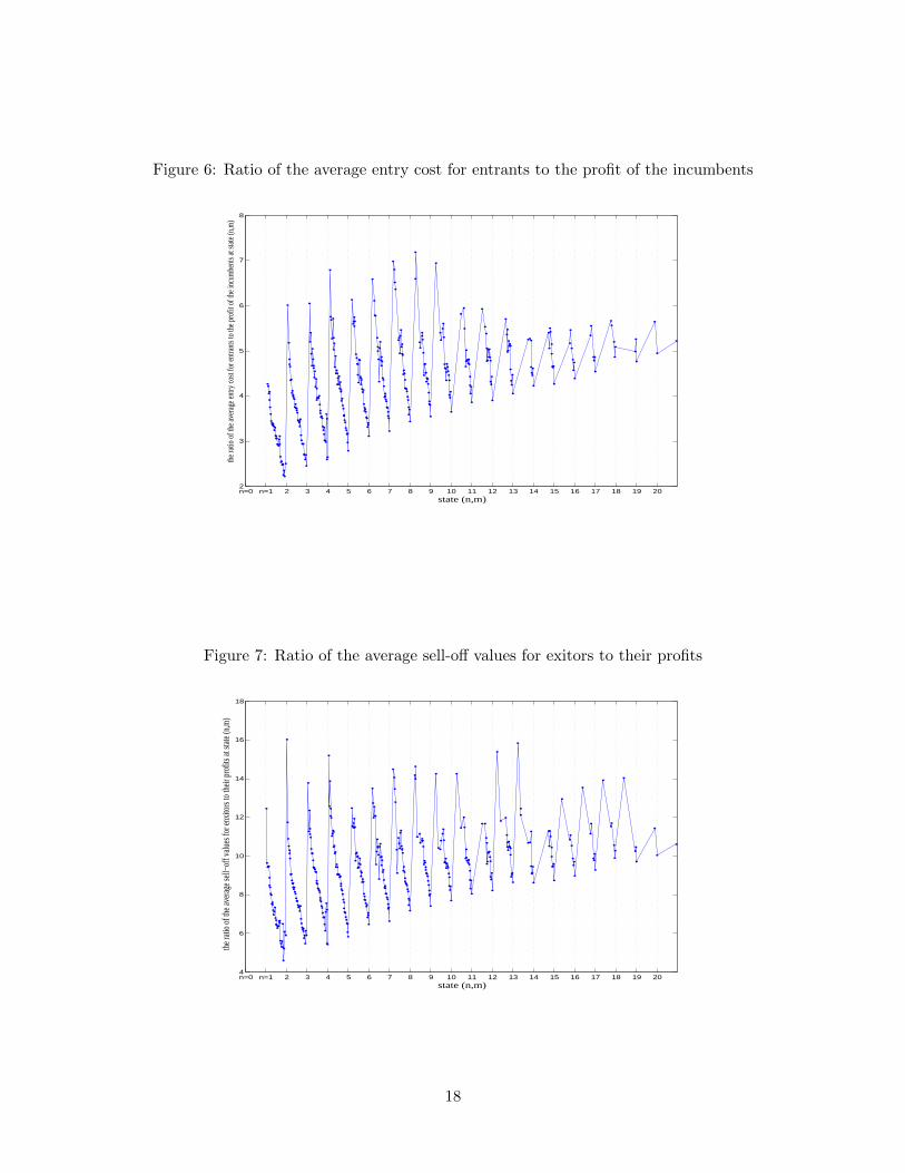
Figure 6: Ratio of the average entry cost for entrants to the profit of the incumbents

n=0 n=1 2 3 4 5 6 7 8 9 10 11 12 13 14 15 16 17 18 19 202

3

4

5

6

7

8

state (n,m)

the r

atio

of th

e ave

rage

entry

cost

for e

ntra

nts t

o th

e pro

fit o

f the

incu

mbe

nts a

t stat

e (n,

m)

Figure 7: Ratio of the average sell-off values for exitors to their profits

n=0 n=1 2 3 4 5 6 7 8 9 10 11 12 13 14 15 16 17 18 19 204

6

8

10

12

14

16

18

state (n,m)

the

ratio

of t

he a

vera

ge s

ell−

off v

alue

s fo

r enx

itors

to th

eir p

rofit

s at

sta

te (n

,m)

18

Figure 8: Fitting of the number of entrants

n=0 n=1 2 3 4 5 6 7 8 9 10 11 12 13 14 15 16 17 18 19 200

0.5

1

1.5

2

2.5

3

3.5

4

4.5

5

state (n,m)

aver

age n

umbe

r of e

ntra

nts a

t stat

e (n,

m)

data

model

Figure 9: Fitting of the number of exits

n=0 n=1 2 3 4 5 6 7 8 9 10 11 12 13 14 15 16 17 18 19 200

1

2

3

4

5

6

state (n,m)

aver

age n

umbe

r of e

xits

at sta

te (n

,m)

datamodel

19

Figure 10: Fitting of the number of entrants (long-run potential entrants)

n=0 n=1 2 3 4 5 6 7 8 9 10 11 12 13 14 15 16 17 18 19 200

1

2

3

4

5

6

7

state (n,m)

aver

age n

umbe

r of e

ntra

nts a

t stat

e (n,

m)

datamodel

Figure 11: Fitting of the number of exits (long-run potential entrants)

n=0 n=1 2 3 4 5 6 7 8 9 10 11 12 13 14 15 16 17 18 19 200

2

4

6

8

10

12

14

state (n,m)

aver

age n

umbe

r of e

xits

at sta

te (n

,m)

datamodel

20