Estimating the Foreclosure Effect of Exclusive Dealing: Evidence

from the Entry of Specialty Beer Producers∗

Chia-Wen Chen†

July 15, 2014

Abstract

This paper estimates an entry model to study the effect of exclusive dealing between

Anheuser Busch and its distributors on rival brewers’ entry decisions and consumer

surplus. The entry model accounts for post-entry demand conditions and strategic

spillover effects. I recover a brewer’s fixed costs using a two-step estimator and find

spillover effects on brewers’ entry decisions. I find that a brewer has higher fixed costs

at locations where Anheuser Busch employ exclusive distributors, but the effect is only

statistically significant in certain local areas. The estimates also show that a brewer

is less likely to enter a location that is farther from its brewery, has lower expected

demand, or is smaller in store size. I implement counterfactual experiments to study

the effect of banning exclusive contracts between Anheuser Busch and its distributors.

The results show that the welfare improvement associated with banning such contracts

is very small.

Keywords: Exclusive Dealing; Foreclosure; Entry; Beer industry.

JEL Classification Numbers: L42; L12; K21

∗I would like to thank Christopher Knittel, as well as A. Colin Cameron, Joonsuk Lee, Julie HollandMortimer, David Rapson, Victor Stango, and three anonymous referees for their valuable comments. I wouldalso like to thank seminar participants at the University of California at Davis, University of Connecticut,University of Leicester, National Taipei University, Academia Sinica, and Shanghai University of Financeand Economics for many helpful comments. I am particularly grateful to John Pauley and The NielsenCompany for allowing me access to the data used in this paper. I also thank James Arndorfer for sharinghis industry insights.

†Contact information: Department of Economics, National Taipei University, 151 University Road, SanShia District, New Taipei City, 23741 Taiwan. Email: cwzchen@mail.ntpu.edu.tw

1 Introduction

An exclusive dealing contract is a vertical agreement between a manufacturer and a dis-

tributor that forbids the distributor from promoting other manufacturers’ products. Such a

contract is controversial in competition policy, because of the potential foreclosure effects.

For example, in 1997 Anheuser Busch launched an incentive program that provided dis-

counts and other benefits to distributors that went exclusively with Anheuser Busch. At

that time, many microbreweries complained they were being dropped by distributors due to

this practice. The theory suggests that exclusive dealing can be efficiency-enhancing, because

it encourages investment in manufacturer-distributor relationships, but it also suggests that

exclusive dealing can be anticompetitive due to raising rivals’ entry costs. In practice, the

extent to which exclusive dealing enhances investments in a vertical relationship or dampens

competition remains an empirical question to be explored.1

This paper examines whether exclusive contracts between a dominant firm and its distrib-

utors have a foreclosure effect. More importantly, by quantifying the magnitude of diverted

sales from a potential foreclosed firm to the dominant firm and the changes in consumer

surplus, this paper looks at the motivations behind exclusive dealing and the welfare impli-

cations from banning such contracts. The empirical setting is the U.S. beer industry. Aside

from mainstream mass producers (Anheuser Busch, Miller, and Coors), many entrepreneurs

entered this industry during the microbrew movement that took off in the 1980s. Most mi-

crobreweries founded during this era were clustered on the West Coast along the “Interstate

5 corridor” from San Francisco to Seattle.2 The boom ended with a shakeout in the late

1990s. One particular factor that may have contributed to the shakeout is Anheuser Busch’s

exclusive dealing program beginning in 1997, which eliminated one of the most dominant dis-

tribution vehicles from its rivals’ choice set. Because there were other distributors available in

the market, the extent of the foreclosure effect requires further examination. The main task

of this paper is to model each specialty beer producer’s entry decision for a location in a set-

1The foreclosure argument led the courts to condemn exclusive dealing contracts between dominant firmsand their distributors after the enactment of the Clayton Act in 1914. However, the Chicago school’sdefense of exclusive dealing started to prevail in the 1970s, and since then the courts have emphasized a ruleof reason approach to such provisions. For earlier cases where the courts were against exclusive dealing, seeStandard Fashion Co. v. Magrane-Houston Co., 258 U.S. 346 (1922) and Standard Oil Co. of Californiaet al. v. United States, 337 U.S. 293 (1949). For decisions favoring exclusive contracts, see Tampa ElectricCo. v. Nashville Coal Co., 365 U.S. 320 (1961) and Beltone Electronics Corp., 100 F.T.C. 68 (1982). InEurope, a recent practice by Intel, which provided rebates and cash benefits to manufacturers and retailers inexchange for purchasing most of their products from Intel, was found to be anticompetitive by the EuropeanCommission and resulted in a e1.06 billion fine in 2009.

2Tremblay and Tremblay (2005) provide an excellent treatment on the history of the microbrewery move-ment. Most specialty beer producers remain microbreweries, but some of them (Boston Beer Company andSierra Nevada Brewing Company) have grown successfully and are no longer microbreweries.

1

ting where their fixed entry costs may be affected by (1) exclusive dealing between Anheuser

Busch and its distributors and (2) spillover effects resulting from other entrepreneurs’ entry

decisions. I then take the estimates from the analysis to perform counterfactual experiments.

This paper contributes to the literature and policy discussion of exclusive contracts in

several ways. First, even though the theoretical literature on exclusive dealing has presented

many fruitful insights, the effect of exclusive dealing is still ambiguous. Empirically, the data

availability problem and the fact that a distributor’s enrollment into an exclusive program

and a brewer’s entry decision are both endogenous to unobserved market conditions have

resulted in few empirical studies in this area. For example, all things being equal, a distrib-

utor that serves an area with a higher demand for domestic products is more likely to enroll

into such a program compared to another one that serves an area with a lower demand for

domestic products. In addition, demand conditions directly affect domestic specialty beer

producers’ entry decisions into a market and result in an endogeneity problem. To this end,

I collect entry data of specialty beer producers and address the endogeneity problem by

controlling for consumers’ demand for beer products in a setting of differentiated products,

which is different from most previous empirical works in this area (Sass 2005; Rojas 2010).3

I show that without accounting for the endogeneity of the exclusivity decision, estimates of

exclusive dealing on the probability of entry are biased upwards.4

Another major contribution of this paper is to take advantage of demand-side estimates

to conduct counterfactual experiments. I study whether a foreclosure-based motivation alone

can rationalize Anheuser Busch’s continuing support for exclusive contracts, as well as to

what extent the consumer surplus would increase if such contracts were banned. Compared

to a previous work (Asker 2005) that tests the foreclosure hypothesis and focuses mainly on

the supply side, this paper quantifies the potential benefits on consumer surplus from banning

exclusive dealing by removing the foreclosure effect and expanding consumers’ choice sets,

which is not directly addressed in the previous literature (Sass 2005; Rojas 2010; Asker 2005;

Chen 2013).5 From an antitrust policy’s perspective, such an estimate of consumer surplus is

3Sass (2005) studies a cross-sectional survey of 381 beer distributors in 1997 and finds that exclusivedealers on average generate higher prices and larger sales for their suppliers, which is more consistent withthe incentive-based theory. Rojas (2010) looks at a scanner dataset of 63 metropolitan areas from 1988 to1992 and uses average exclusive dealing intensity that a brand has in other cities in the same region as aninstrumental variable for the exclusive dealing decision. He finds that exclusive dealing increases consumers’willingness to pay and provides a cost advantage for firms.

4Another possible source of endogeneity is the extent to which a distributor can effectively increase localdemand over its products due to legal restrictions. For example, Sass (2005) considers state laws banningoutdoor advertising of malt beverages and argues that these laws influence participation in the exclusiveprogram across states. In this paper, I do not address this kind of endogeneity because this paper’s empiricalsetting is entirely in Northern California, and so the legal environment is more homogeneous than the oneconsidered in Sass (2005).

5When products are differentiated, the introduction of new products with quality improvements can

2

crucial in evaluating vertical restraints in the marketplace. I show that even when efficiency

gains from exclusive contracts are not acknowledged and even when exclusive contracts have

raised rivals’ entry costs in some local areas, if the antitrust agency adopts a consumer

surplus standard (as it currently does) rather than a total welfare standard to evaluate

vertical restraints, then policy intervention in banning such contracts may be ineffectual.6

Inferences about the foreclosure effect through direct comparisons of entry patterns can

suffer from omitted variable bias, because post-entry market outcomes may differ across

locations and firms. Thus, I estimate the demand for beer to construct counterfactual

expected post-entry sales. With the panel structure of the dataset, I can control for invariant

brand and location fixed effects. I estimate the demand system using a nested logit model.

The model allows the substitution patterns to vary based on product segments (e.g., country

origin or style of beer) and has more reasonable substitution patterns than a simple logit

model.7

This paper also builds on empirical studies that estimate static entry games. Bresnahan

and Reiss (1991) show how to estimate an equilibrium model of entry for symmetric firms

with data on market characteristics and the number of firms. Similar to Bresnahan and

Reiss (1991), I allow both total variable profits and fixed costs to depend on the number

of brewers. Moreover, given that I observe a pool of global potential entrants, along with

their actual sales and entry patterns, my model allows heterogeneous brewers to produce

differentiated products with different fixed costs.8

Following recent developments in estimating strategic games (Seim 2006; Augereau,

Greenstein, and Rysman 2006; Ellickson and Misra 2008; Sweeting 2009; Bajari, Hong,

Krainer, and Nekipelov 2010), I model the entry behavior of specialty beer producers using

an incomplete information framework that helps to incorporate a large number of players in

the game. In this setup, a brewer’s entry decision depends on the expected market profitabil-

ity and private information. I estimate the model following a two-step estimation procedure,

similar to that of Ellickson and Misra (2008) and Bajari, Hong, Krainer, and Nekipelov

improve consumer surplus significantly, and counterfactual analysis based solely on a single dimension (theaverage price or an aggregate sales measure) may underestimate the foreclosure effects on consumer welfare.

6I thank anonymous referees for directing me to a consumer surplus approach and for pointing out that ifAnheuser Busch adopts an exclusive contract for efficiency reasons, then equilibrium prices are likely to belower. If this is the case, one can interpret the result in this paper as that the collateral damage in blockingsome craft breweries from operating is small.

7The nested logit model has wide applications in estimating transportation and energy demand and isalso applied to other industries such as automobiles, movies, home videos, and banking (Goldberg 1995;Einav 2007; Chiou 2008; Dick 2008). In particular, Ho, Ho, and Mortimer (2012) estimate a nested logitmodel in the context of empirical analyses of vertical contracts.

8Berry (1992) first estimates a model of entry in the airline industry that allows for firm heterogeneity infixed costs. This present paper exploits data on beer prices and sales and allows a firm’s variable profits toalso depend on rivals’ identities.

3

(2010), and use the demand estimates to control for post-entry sales. The estimation is done

in three steps. The first step estimates the equilibrium entry probabilities implied by the

model. The second step estimates the demand for beer. Using the demand estimates and

the beliefs about rivals’ entry probabilities, I construct expected post-entry sales. The third

step then plugs the above estimates into the likelihood function to recover a brewer’s fixed

costs.

Economic theories vary in their explanations of exclusive contracts. Traditionally, the

Chicago school has argued that exclusive dealing cannot be used as a device for monopo-

lization (Posner 1976; Bork 1978): if the sole purpose of exclusive contacts were to restrict

competition, then downstream buyers would never sign them in the first place, because do-

ing so would only lower the potential total surplus. Incentive theories show that exclusive

dealing enhances incentives for investment when investments made by parties in a bilat-

eral relationship have external effects on outside parties (Marvel 1982; Klein and Murphy

1988; Besanko and Perry 1993; Martimort 1996; Bernheim and Whinston 1998; Segal and

Whinston 2000a).9

Anticompetitive arguments focus on the foreclosure effect of exclusive dealing. In this

literature, manufacturers either sign exclusive contracts with lower-cost buyers, trying to

raise their rivals’ costs, or with a large number of buyers, trying to foreclose the market

directly when facing minimum economies of scale.10 Segal and Whinston (2000b) point out

that whether manufacturers can successfully carry out the above “naked exclusion” scheme

depends on how well they are able to exploit the coordination problem faced by buyers.11

Most previous studies of exclusive dealing in the U.S. beer industry find efficiency reasons

more consistent with empirical evidence (Sass 2005; Rojas 2010; Chen 2013). Specifically, us-

ing variation generated from distribution contract changes, Chen (2013) finds that a brand’s

market share is higher when the brand’s distributor has fewer external trading opportuni-

ties.12 Nevertheless, most of the above papers assume products are homogeneous and do

9In fact, Segal and Whinston (2000a) show that restricting a distributor’s external trading opportunitiesincreases the level of investment when a distributor’s investment has a substitutable effect, i.e., investmentdevoted to one brand hurts the value of other brands in the same distribution network; or when a manufac-turer’s investment has a complementary (positive spillover) effect.

10Salop and Scheffman (1983), Aghion and Bolton (1987), Rasmusen, Ramseyer, and Wiley (1991), andBernheim and Whinston (1998) provide theoretical foreclosure arguments for exclusive dealing. For a recenttheoretical treatment on vertical exclusion without an explicitly written exclusive contract, see Asker andBar-Isaac (2014).

11Simpson andWickelgren (2007), Abito andWright (2008), and Doganoglu andWright (2010) also providesettings that allow exclusive dealing to achieve inefficient outcomes. Simpson and Wickelgren (2007) andAbito and Wright (2008) consider the case when buyers compete, and Doganoglu and Wright (2010) studyexclusive contracts under the network effect.

12Chen (2013) exploits a distribution deal between Anheuser Busch and InBev in 2007 to study the effect ofallowing more brands to have access to exclusive distribution networks on brand level outcomes in Northern

4

not speak to the effect of exclusivity on consumer surplus and its foreclosure effect when

products are differentiated, which is the main focus of this paper.

There is a growing empirical literature on estimating industry models with vertical re-

straints (in particular, Asker 2005; Ho, Ho, and Mortimer 2012; Crawford and Yurukoglu

2012; Lee 2013; Conlon and Mortimer 2013; Sinkinson 2014).13 More closely related to my

paper is Asker (2005), who also studies exclusive contracts in the beer industry and takes a

structural approach in a differentiated product framework to recover the costs incurred and

the promotional efforts made of distributors in exclusive and less exclusive markets. Asker

(2005) finds that distributors in less exclusive markets are not more efficient than distributors

in exclusive markets and rejects the foreclosure hypothesis. Even though the main focus of

Asker (2005) is on the supply side, the beer products in his analysis are mainly produced by

domestic or foreign mass-producers, which are unlikely to be forced out of the market due to

exclusive dealing in the first place. By contrast, the structural approach in this paper allows

me to directly look at the entry patterns of firms that are more likely to be foreclosed, and

more importantly, to estimate the effect of banning exclusive dealing on consumer surplus.

I find that the demand for beer is elastic and that the price of a specialty beer product

is lower at locations closer to its producer’s establishment. Controlling for prices, I also find

that consumers enjoy a product more if it is locally brewed. These findings explain why

most specialty beer producers are not present in every location. I then take the demand

estimates to the model of entry. When strategic interactions are not allowed in the model,

exclusive dealing shows no impact on a specialty beer producer’s entry decision. Once

strategic interactions are allowed, I find that in some local markets, a store with an Anheuser

Busch exclusive distributor is associated with a reduction of 6 percentage points (21%) in a

specialty beer producer’s entry probability, suggesting a foreclosure effect due to exclusive

dealing. I also show that a specialty beer producer has lower fixed costs at a location where

the number of rivals is larger. The result implies that firms can benefit from clustering

their strategic decisions, which is similar to the findings in previous studies that estimate

strategic effects, such as Ellickson and Misra (2008), Sweeting (2009), Bajari, Hong, Krainer,

and Nekipelov (2010), and Vitorino (2012).

Finally, I use demand estimates to carry out counterfactual experiments that remove

exclusive dealing. The magnitude of the foreclosure effect is too small to claim that Anheuser

California. The result suggests InBev brands’ market shares to be higher once they were allowed access toAnheuser Busch’s exclusive distribution networks. In addition, other brands’ market shares were lower whentheir distributor gained InBev products. The results are consistent with an incentive-based explanation forfirms preferring exclusive contracts.

13For a thorough review of earlier empirical studies on vertical integration and vertical restraints, seeLafontaine and Slade (2007) and Lafontaine and Slade (2008).

5

Busch’s exclusive dealing program is entirely driven by a foreclosure motivation. Thus, the

decrease in entry probabilities in some local markets is more likely to be a side-effect of

exclusive contracts. I do not find much change in welfare due to banning exclusive dealing

contracts between Anheuser Busch and its distributors. In fact, I show that adding more

specialty brands does not provide much benefit to consumers: when exclusive dealing is

removed in a market, the change in aggregate consumer welfare is only $15 per store per

quarter. This result, complemented by the findings from Sass (2005), Rojas (2010), and Chen

(2013) supporting the efficiency motives behind exclusive dealing, reinforces that banning

exclusive contracts in the current beer industry is hardly welfare improving.

This paper proceeds as follows. I begin by examining the industry and the data. I

then describe the model of demand and entry behavior. Next, I discuss the corresponding

estimating procedures and identification issues. Finally, I present the empirical results and

discuss the implications and potential future research.

2 Industry Background

The U.S. beer industry has nearly 3,000 brewing establishments and accounts for approx-

imately $100 billion in annual sales.14 During the sample period of the data (2006-2008),

Anheuser Busch, Miller, and Coors collectively held nearly 80% of the market, with An-

heuser Busch being the most dominant firm in the industry (50% market share).15 Since

the end of Prohibition, the industry has been heavily regulated by state laws, under which

vertical integration between manufacturers, distributors, and retailers is not allowed. The

vertically-separated “three-tier system” (manufacturing, distribution, and retailing) is one

of the main features of the beer industry.16

Beer manufacturers rely on distributors to transport and rotate their products in local

markets so as to guarantee product availability and freshness. Distributors are also respon-

sible for point-of-sale promotional activities. Building and maintaining good relationships

with distributors to receive adequate promotional support are thus vital to a brewer’s suc-

cess, especially when it comes to entering a new market or launching a new advertising

campaign. While a brewery would prefer its distributors to be exclusive and to devote as

much promotion efforts to its products as possible, it may not be in the best interest of dis-

14Statistics are obtained from the Beer Institute website.15The industry has become even more concentrated after two mergers in 2008. Miller and Coors formed

a joint venture. Anheuser Busch then merged with InBev, the biggest brewer in Europe.16The extent to which administrators regulate alcoholic beverages vary by state and in alcohol content.

For beer, most states regulate private licensed retailers and distributors and adopt the three-tier system torestrict private ownership across different tiers. For wine and spirits, several so-called control states buyalcohol directly from manufacturers and act as monopolies in the wholesale and retail distribution tiers. Forrecent studies that examine possible welfare losses created by state regulations on alcoholic beverages, seeSeim and Waldfogel (2013), Miravete et al. (2014), and Conlon and Rao (2014).

6

tributors to build a relationship with just one brewery. To maintain a stable cash stream and

warehouse/route efficiency, a distributor is more likely to prefer having all the best-selling

products in its brand portfolio. Conflicts of interest handling multiple brands from com-

peting breweries at the same time often render lower promotional efforts than what would

be considered optimal from a brewer’s perspective. One of the main efficiency arguments

for exclusive dealing is to create a loyal vertical relationship and enhance a distributor’s

promotional investments.17

The beer industry is divided into three segments: domestic macro brands, imported

brands, and specialty brands. The top three domestic mass-producers (Anheuser Busch,

Miller, and Coors) focus on “regular domestic beer,” which are mainstream, lower-priced,

light lager products with large package size options. Imported brands include products

(usually well-established ones) from foreign countries that are typically priced higher than

domestic beer. The last category, domestic specialty brands, refers to domestic brands

that emphasize flavor and taste. According to Tremblay and Tremblay (2005), specialty

beer producers emulate the business model of wineries in Northern California by providing

“boutique” products in small batches. They advocate the taste of “real beer” and encourage

consumers to choose craft beer instead of beer that contains a high concentration of adjuncts

and that lacks flavor. Sierra Nevada Brewing and Boston Beer Company are pioneers of the

microbrewery movement during the 1980s and are the most successful and nationally known

companies in this segment.

Most firms of specialty beer products enjoy a higher market share in geographic areas

closer to their brewery, which is consistent with Bronnenberg et al. (2009).18 Taking Sierra

Nevada Brewing as an example, while it has a 1% market share across all stores in the

sample data, in Chico, California where its brewery is located, it has an average 8% market

share, putting it very close to Anheuser Busch’s market share (9% in Chico, 10% overall).

Because Sierra Nevada is so successful in Chico, one might presume that it would be difficult

for other microbreweries to break into store shelves there. However, the store that carries

17Both manufacturers and distributors can make investments to enhance the value of their relationships.For example, a brewer can provide training programs on consumer behavior for distributors. Similarly, adistributor can make efforts to secure better shelf space for its brewers. These investments not only increasethe value of vertical relationships, but also alter bargaining positions between the parties involved. In theformer case, if training lessons are not specific to the relationship, then providing training lessons may hurta brewer’s ex-post bargaining power. On the contrary, if promotional efforts are tailored to a brewer, thensuch investments can hurt a distributor’s ex-post bargaining power. Segal and Whinston (2000a) point outthat when investments have external values and are not contractible, exclusivity can lead to a higher levelof investments under some circumstances. Therefore, an important motivation for exclusive dealing is toaddress the incentive problems in vertical relationships.

18Bronnenberg et al. (2009) find an early entry advantage for several consumption goods, such as beer,coffee, and mayonnaise. The order of entry into a market is correlated with the rank of market share andperceived product quality.

7

the most number of California specialty beer brands is also in Chico (39 brands per store on

average, compared to 24 brands per store on average). In this specific case, the entry of a

rival microbrewery does not seem to create an entry barrier for other firms. In the empirical

setting, a potential spillover effect is taken into account by allowing fixed costs to depend

on the expected number of specialty beer producers. I also allow a “locally brewed” effect

when I estimate consumers’ demand for beer and consider the possibility that the distance

between a grocery store and a product’s brewery does affect the entry pattern of specialty

beer producers.19

In response to consumers’ demand for specialty brands, top domestic mass-producers ac-

quired several microbreweries and introduced their own brands of specialty beer in the late

1990s. Anheuser Busch launched an incentive program during the late 1990s, called “100

percent share of mind.” The program provided discounts and other benefits for distributors

in exchange for exclusivity with Anheuser Busch. As a result, many brands of other brew-

eries were dropped by their Anheuser Busch distributors. Figure 1 illustrates the impact of

Anheuser Busch’s exclusive dealing program in the three-tier system. In panel (a), specialty

and imported products are allowed to share distribution networks with Anheuser Busch. It

presents that Microbrewery 1 chooses to hire an Anheuser Busch distributor while Micro-

brewery 2 chooses to work with a Miller distributor. In panel (b), because the Anheuser

Busch’s distributor is exclusive, all of the specialty and imported products that are not affil-

iated with Anheuser Busch are squeezed out of Anheuser Busch’s distribution network and

are crowded out to other distribution networks.

Given that the other two leading brewers (Miller and Coors) rarely share distribution net-

works with Anheuser Busch, exclusive dealing cannot completely foreclose all distribution

channels. Nevertheless, Anheuser Busch’s exclusive dealing program may raise distribu-

tion costs for potential entrants by (1) enhancing rival distributors’ bargaining power and

by (2) forcing rival brewers to use less efficient distributors, thus reducing the likelihood

of entry events. When most of the specialty and imported brands from competing brew-

eries are crowded out into one distribution network, it enhances the distributor’s bargaining

power, which raises the entry barrier for a prospective microbrewery into a new market.

The crowding-out effect also intensifies incentive conflicts within a distribution network and

may drive a distributor’s promotional efforts of a brand further away from its optimal level.

Finally, exclusive dealing may raise rivals’ costs by forcing them to team up with smaller or

less efficient distributors, because Anheuser Busch is the biggest competitor in the industry

and its distribution networks are often viewed as a superior promotional vehicle due to its

19The dummy variable “locally brewed” is set to be 1 when the brewery is located within a 10-mile radiusof a store.

8

economies of scale in distribution.20

3 Data

The scanner dataset is provided by Nielsen. The dataset contains weekly price and sales data

of the malt beverage category for all stores of a major grocery chain in Northern California

from April 2006 to April 2008. The original dataset comes at the Universal Product Code

(UPC) level, which includes all sales records from all packaging options for all brands. I

collapse the data to a quarterly brand level to take into account that some specialty brands

may have very little (or even no) sales within a week or a month at the UPC level, and

because the demand estimates from quarterly data are more likely to be suitable for policy

analysis.21 I search a product’s website for information on the product’s country of origin

(domestic or foreign) and product ownership. For domestic specialty beer producers, I

calculate the distance from a store to the firm’s nearest establishment (brewery or brewpub)

using Google’s map service. I also collect data on local contract rents at the zip code area

level (“Gross Rent”) from Census 2000 as a further control for a location’s fixed costs.22

The scanner dataset also includes a product category variable, made up of light, lager,

ale, stout/porter, malt liquor, and non-alcoholic (alcohol by volume of less than 0.5%) beer,

and three categories for alternative malt beverage. Due to product similarity, I assign all

alternative malt beverages to one style (alternative) and generate a new style specifically for

domestic mainstream lager products.23 In this way, I end up with eight different product

styles.

Data on Anheuser Busch exclusive distributors and their territories are from the Cali-

fornia Beer and Beverage Distributors (CBBD) annual member directories. Each directory

contains a list of each member distributor’s representative brewers and the counties it oper-

ates within California.24 Table 1 lists some typical entries from the 2006 CBBD directory,

with California specialty beer producers that are matched to the scanner dataset denoted by

bold type. Most distributors represent at least one of the domestic macro brewers (Anheuser

20Economies of scale are important in distribution. For example, Bump Williams, an IRS industry analyst,notes that “there’s nobody better than these three networks (Anheuser Busch, Coors, and Miller). Theycan get these beers on shelves overnight.” See Kesmodel (2007).

21I divide total revenue during a quarter by the number of six-packs sold during a quarter to calculate aproduct’s price at the quarterly level. When products are storable goods, using temporary price promotionsin weekly data to identify price elasticities can lead to an overestimation of price sensitivity (Hendel andNevo 2006).

22In Census 2000, “Gross Rent” is defined to include “contract rent and estimated average monthly costof utilities (electricity, gas, water, and sewer) and fuels (oil, coal, kerosene, wood, etc.) if these are paid bythe renter.”

23I define a product to be domestic mainstream lager if it is a lager product from one of the three biggestdomestic competitors in the industry and has large package size options.

24The 2006 and 2007 trade directories were provided by local distributors.

9

Busch, Miller, and Coors) and also carry other imported brands and domestic specialty

brands. In addition, there are independent distributors that do not carry any brands from

domestic macro firms, but collect a large number of specialty or imported brands.

3.1 Store Attributes

Table 2 provides the attributes of stores that carry the highest/lowest number of California

specialty beer producers. The top 10 stores with the highest number of California specialty

beer producers have on average 12.3 firms, of which the minimum quantity of six-packs sold

per store during a quarter is 15.4 units. On the other hand, the bottom 10 stores with the

lowest number of California specialty beer producers have on average 5.4 firms, of which the

minimum quantity of six-packs sold per store during a quarter is 43.4 units. The minimum of

six-packs sold per store can be interpreted as a rough index for a store’s entry threshold, and

it appears that stores with more firms have a lower entry threshold (as opposed to having

a bigger market). Moreover, because it is unlikely that price-cost margins would increase

with the intensity of retail competition, variation in entry thresholds is most likely driven

by variation in fixed costs.

Figure 2 shows geographic areas that include stores from the grocery chain studied in this

paper and also presents Anheuser Busch distributors’ exclusivity status. Table 3 shows the

means and standard deviations for store attributes. I provide summary statistics for stores

with Anheuser Busch non-exclusive distributors and stores with Anheuser Busch exclusive

distributors. About 17% of the stores are located in counties in which Anheuser Busch has

exclusive distributors. On average, these stores have more California specialty beer producers

entering the markets and generate more sales. Therefore, it appears that exclusive dealing

has no anticompetitive effect on a firm’s entry decision. However, Table 3 also shows that

store attributes and demographics differ across the two types of stores. Inferences about

the foreclosure effect directly from Table 3 can thus suffer from omitted variable bias. For

example, suppose Anheuser Busch is more likely to hire exclusive distributors where the

demand for beer is higher. If higher demand also leads to more entrants, then our simple

comparison will push the exclusive effect to be biased upward (less foreclosure).

To deal with the potential problem from omitted variable bias, the empirical strategy to

identify the exclusive effect in this paper is to first control for firm specific post-entry sales

by estimating the demand for beer. In addition, I control a firm’s fixed entry costs at a

location by using the size of the store’s physical selling area, gross rents in the store’s zip

code area, the distance between a store and a product’s brewery, and the expected number

of rivals.

10

3.2 Entry Variation

There are 32 specialty beer producers in the data, and 26 of them are California-based firms.

Many firms cluster their breweries around the San Francisco Bay Area and Sacramento. I

tabulate their entry patterns in Table 4 to show variation in the data. From the table, firms

vary by the number of stores they enter. Some firms enter all 229 locations, but then there

are also firms that are more local and have sales at fewer than 10 stores. Moreover, breweries

from other states are more likely to be well-established ones and on average enter more stores

than local firms. As will become clearer in the empirical estimation, I use the distances from

breweries to stores as exclusion restrictions to identify the strategic entry effect. Because the

distances from stores to the main breweries of non-California firms are extremely far, I only

consider the entry decisions of California specialty beer producers in the empirical section.

4 Model

4.1 Demand Side

A consumer’s decision problem for purchasing a beer product is modeled using a discrete

choice model. Each consumer is presented with different types of beer with various quality

levels and is assumed to decide whether or not to purchase one unit of beer.25 Consumers

are differentiated by the markets where they live, and their preferences for different types

of beer. In particular, consumer c purchasing product j in market t receives a mean utility

term δjt and an idiosyncratic term νcjt. The utility from consuming beer is:

ucjt = δjt + νcjt.

When νcjt is independently distributed with Type 1 extreme value distribution, the model is

a logit model that offers easy tractability. Nevertheless, the logit specification is well-known

to produce unrealistic substitution patterns driven by market shares instead of product

similarities.

To allow for more plausible substitution patterns, the independence assumption for νcjt

can be relaxed by introducing random coefficients on product attributes. In particular, a

nested logit model allows νcjt to include correlated shocks from different market segments,

and so a consumer who purchases a certain type of beer will be more likely to substitute

it for products with similar attributes. Similar to Chiou (2008), I use a four-level nested

structure, which is shown in Figure 3. The nesting is consistent with the data that have a

category variable (beer style) and the industry practice that uses products’ country of origin

(domestic/imported) for market segmentation. I allow the correlated shocks for consumer

25A unit is defined as a six-pack of beer (72 ounces in total).

11

c to come from three possible sources: a shock, ζb, for all beer products; a shock, ζd, for

all products in domestic group d; and a shock, ζg, for all products under a specific domes-

tic/foreign beer style g. Following Cardell (1997), the error structure of a nested logit model

can be decomposed as:

νcjt = ζcb + λ3ζcd + λ2λ3ζcg + λ1λ2λ3ωcjt,

where ω is independent and identically distributed with Type 1 extreme value, and the

correlated shocks ζ are from a distribution, such that if ω is distributed with Type 1 extreme

value, then ζ + λω is also distributed with Type 1 extreme value when 0 < λ ≤ 1.

The λ terms measure how products in the same category are independent of each other:

when all λs approach to 1, all shocks are independent and the model reduces to a simple

logit model. The nested logit model is basically a random coefficients model with coefficients

on group dummy variables, which allows the correlation to be higher within a group and

still preserves the closed-form tractability similar to a logit model.

The mean utility of product j in market t is specified to be:

δjt = xjβ − α pjt + γAjt + ξjt,

where xj includes observed fixed product attributes such as alcohol by volume and calories,

pjt is the price, and ξjt is the unobserved (by an econometrician) advantage for brand j in

market t. To allow preferences for local products, I include a dummy variable Ajt, which

is equal to one if the product is locally brewed (the distance between a store and a brand’s

brewery is less than 10 miles). In the estimation, I include brand, store, and quarter dummies

to absorb invariant product and market attributes. Consumers are allowed to not purchase

any product presented in the model. The mean utility from purchasing an outside good is

normalized to zero.

The mean utility can be recovered using Berry (1994)’s inversion technique:

ln(sjt)− ln(s0t) = xjβ − α pjt + γAjt + (1− λ1λ2λ3) ln(sj|g) + (1− λ2λ3) ln(sg|d)(1)

+ (1− λ3) ln(sd|b) + ξjt,

where sjt and s0t are the respective market shares for product j and the outside good, sj|g

is the market share for brand j as a fraction of the market share of group g, sg|d is the

market share for group g as a fraction of the market share of the domestic/foreign product

group, and sd|b is the market share for the domestic/foreign product group as a fraction of

the market share of all beer products.

12

The market share of product j is the probability that product j is chosen by consumers.

In a nested logit model, there is a closed-form solution for the choice probability. First, I

decompose the choice probabilities (market shares) into conditional probabilities (omitting

subscript t):

(2) sj = sj|g × sg|d × sd|b × sb,

where sb is the probability of choosing the inside good. Following McFadden (1978), the

inclusive values for each nest are defined as

I1g ≡ log(∑

j∈Ggexp( (xjβ − α pjt + γAjt)/λ1λ2λ3 )

)I2d ≡ log

(∑g∈Dd

exp(λ1I1g))

I3 ≡ log(∑

d∈B exp(λ2I2d)).

I then express the conditional probabilities as:

sj|g =exp( (xjβ − α pjt + γAjt)/λ1λ2λ3 )∑

k∈Gg

exp( (xkβ − α pkt + γAkt)/λ1λ2λ3)(3)

sg|d =exp

(λ1I1g)∑

l∈Dd

exp(λ1I1l)

sd|b =exp

(λ2I2d)∑

m∈Bexp

(λ2I2m)

sb =exp(dqzq + dszs + λ3I3)

1 + exp(dqzq + dszs + λ3I3),

where zq and zs are the respective dummy variables for quarters and stores, and dq and ds are

the corresponding coefficients that do not vary for all inside goods. Moreover, Gg, Dd, and

B are the sets of all products in domestic/foreign beer style group g, in domestic/foreign

group d, and in the inside good group B, respectively. Combining (2) and (3) gives the

choice probability of product j as a function of model parameters.

4.2 Entry Game

Following the setup in Bajari, Hong, Krainer, and Nekipelov (2010), I model a specialty beer

producer’s entry decision using a static discrete choice model with private information. In

13

each period, N potential entrants make entry decisions to different locations simultaneously.26

Let ai denote firm i’s entry decision, where ai is equal to one if it enters, and ai is equal to

zero if it does not enter. Let a−i denote rivals’ action profile (a1, ...ai−1, ai+1..., aN). Let s

denote public state variables, commonly known by all firms and econometricians, and let ϵi

denote firm i’s private information. Following the literature, I assume private information

shocks are independent and identically distributed from a known distribution.

Firm i’s period utility function is a function of its own action, ai; rival firms’ action

profile, a−i; state variables, s; its private information, ϵi; and model parameters, θ. The

period utility function can be expressed as:

ui(ai, a−i, s; θ) = πi(ai, a−i, s; θ) + ϵi(ai),

where

πi(ai, a−i, s; θ) =

{Vi(a−i, s; θ)− Fi(a−i, s; θ) if ai = 1

0 if ai = 0,

and Vi(a−i, s; θ) and Fi(a−i, s; θ) are firm i’s variable profits and fixed costs, respectively. In

the specification, both variable profits and fixed costs depend on rivals’ actions.27 I assume

demand shocks are realized after a firm’s entry decisions, which is a standard approach used

in the literature.28 Under this assumption, firms receive demand shocks for each brand after

they have committed to their product choices. Still, when product entry is endogenous, the

obtained price elasticities are likely to be biased and misleading (Musalem and Shin 2013).

I return to the discussion of endogenous product entry in the appendix.

Since firm i does not observe its rivals’ private shocks, firm i’s decision rule is a function

of state variables and its own private information. Therefore, the entry probability of firm i

conditional on state variables is an integral of the decision rule over all possible values of ϵi

26It is worth noting that in reality, an entry decision is never determined solely by brewers, but rather isan outcome jointly determined by the actions of brewers, distributors, and retailers. In fact, when interestedin a market, a brewer needs to contact distributors in that area to see whether a distribution contract canbe reached. Even though a brewer assigns a distributor in an area, this does not guarantee its products’penetration to all of the distributor’s retail accounts. A brewer still needs to constantly work with thedistributor and different retailers to make sure its products are properly promoted. Because a full-fledgedmodel of the search and negotiation process between manufacturers, distributors, and retailers is out of thescope of this paper, I assume that manufacturers know the demand conditions and fixed costs involved inentering a market prior to their entry decision and make decisions accordingly.

27In the current static setup, I cannot distinguish between sunk entry costs and fixed costs that are notsunk. The estimated fixed costs are a combination of both types of costs.

28For instance, in Eizenberg (2014)’s study of the home personal computer market, even though productline configurations are allowed to be endogenous, firms are assumed to only observe the realization of de-mand shocks after they make product line configuration decisions. As discussed in Eizenberg (2014), thisassumption can be further relaxed to allow firms to forecast systematic demand effects, as long as theseeffects are controlled for in the demand estimation (using store or brand fixed effects).

14

weighted by the density of ϵi.

Let σi(ai = 1|s) denote firm i’s entry probability conditional on state variables, and let

σ−i(a−i|s) =∏

j =i σj(aj|s) denote the probability of an action profile from rivals. Firm i

chooses to enter a location if:∑a−i

πi(ai = 1, a−i, s; θ)σ−i(a−i|s) + ϵi(ai = 1) > ϵi(ai = 0).

If we assume private information shocks are distributed with Type 1 extreme value distribu-

tion, then equilibrium entry probabilities from a Bayesian Nash Equilibrium are:

(4) σi(ai = 1|s) =exp(

∑a−i

πi(ai = 1, a−i, s; θ)σ−i(a−i|s))1 + exp(

∑a−i

πi(ai = 1, a−i, s; θ)σ−i(a−i|s)), for i = 1, ..., N.

Equation (4) implies that given any set of parameters, the optimal entry probabilities need

to satisfy a fixed point condition. In his work studying a dynamic programming model, Rust

(1987) shows one can estimate an equation similar to equation (4) with a nested fixed point

algorithm (NFXP). Specifically, for any set of parameters, a NFXP algorithm searches for

the implied fixed point (conditional choice probabilities) in (4) to construct the likelihood.

Thus, it requires solving a fixed point for many values of parameters. Moreover, constructing

the likelihood under the case of multiple equilibia requires specifying an equilibrium selection

mechanism.

To reduce the computation burden from a NFXP algorithm, Aguirregabiria and Mira

(2002) propose a two-step approach. Instead of assuming the equilibrium is unique or em-

ploying a specific equilibrium selection mechanism, the two-step approach only requires that

the equilibrium played in the data does not switch.29 In the first step, a researcher estimates

the consistent choice probabilities conditional on observed states. In the second step, the

researcher then recovers the parameters of the utility function conditional on these choice

probabilities.30

I now turn to the specifications of the variable profits and the fixed costs in order to

estimate the model. For each rival action profile, there is a corresponding variable profit

29This assumption is less restrictive when more data on specific markets are available. For example, withdetailed cross-sectional data, Ellickson and Misra (2008) adopt a two-step estimator and estimate each firm’sbeliefs by pooling observations with similar characteristics across markets. In contrast, I employ a paneldataset that allows me to estimate the entry probabilities of rivals market-by-market, and so the assumptionmade in this paper is even weaker than Ellickson and Misra (2008).

30The two-step approach leads to many applications in dynamic games such as those in Bajari, Benkard,and Levin (2007) and Pakes, Ostrovsky, and Berry (2007).

15

Vi(a−i, s; θ) for firm i when it enters a market. I specify Vi(a−i, s; θ) as:

Vi(a−i, s; θ) = mi Si(a−i, s; θ),

where Si(a−i, s; θ) is the total units of sales for firm i (in terms of the number of six-packs),

and mi is firm i’s variable profits per unit of sales. Total units of sales of firm i are:

Si(a−i, s; θ) =∑j∈Fi

Ms sj(a−i, s; θ),

where Fi is the set containing all products from firm i, sj is the market share for product j,

and Ms is the potential market size of store s. Note that in this specification a firm’s average

variable profit does not vary according to the identity of rivals or locations. The underly-

ing assumptions are that the number of specialty beer producers does not have immediate

effects on the equilibrium prices upon entry and a firm’s average variable profit is constant

across stores. Given that specialty beer producers are fringe firms in each market, it is not

unreasonable to assume that the presence of rivals in this segment does not have much effect

on other firms’ pricing strategy and that these firms have relatively the same margins across

stores.

Similar to Bresnahan and Reiss (1991), I allow later entrants to have different fixed costs

than incumbents have and use the following specification for the fixed costs:

(5) Fi(a−i, s; θ) = di + s′η + τ

∑j =i

1{aj = 1}.

As Bresnahan and Reiss (1991) discuss in their paper, τ is positive when later entrants are

less efficient or face entry barriers, and they impose τ to be positive in their estimation.

However, since the industry context in this present paper is very different from theirs, I do

not restrict τ to be positive.31 The state variables s entering into equation (5) include factors

that affect access to distributors and to shelf space after controlling for post-entry variable

profits. In the estimation, the above state variables s include each firm’s distance from a

store to its brewery, the size of a store’s selling area, and the presence of an Anheuser Busch

exclusive distributor. Firm fixed effects, di, are also included to allow for firm heterogeneity.32

31Bresnahan and Reiss (1991) look at the entry behaviors of doctors, dentists, druggists, plumbers, andtire dealers.

32Here, the distance variable is used to capture fixed costs associated with entering into a new market.Factors that affect a firm’s variable profits in a distant market are controlled for by using “predicted price”and “locally brewed” variables obtained from the demand estimation.

16

Using the specifications for the variable profits and the fixed costs, equation (4) becomes:

σi(ai = 1|s) =exp

(mi

∑a−i

Si(a−i, s; θ)σ−i(a−i|s)− (di + s′η + τ

∑j =i

σj(aj = 1|s) ))

1 + exp(mi

∑a−i

Si(a−i, s; θ)σ−i(a−i|s)− (di + s′η + τ∑j =i

σj(aj = 1|s) )) ,

for i = 1, ..., N.(6)

For each location, the final state variables s in equation (6) are the store’s potential market

size, each product’s attributes, each firm’s distance from the store to its brewery, the size of

the store’s physical selling area, and whether Anheuser Busch has an exclusive distributor.

Parameters θ include the demand-side parameters and the supply-side parameters. Demand-

side parameters are marginal utility of income, α; marginal utility of fixed product attributes,

βj; marginal utility of the locally brewed product, γ; and the inclusive values from the nested

logit model, λ1, λ2, and λ3. Supply-side parameters are each firm’s variable profit per unit

(mi), and the fixed cost parameters (di, η, and τ) are firm fixed effects, store size, distance

from stores to breweries, the presence of an Anheuser Busch exclusive distributor, and the

strategic effect on fixed costs.

Ellickson and Misra (2008) and Bajari, Hong, Krainer, and Nekipelov (2010) both esti-

mate a static game using a two-step approach. They first estimate firms’ beliefs about the

choice probabilities and then maximize the pseudo likelihood function. Following the same

approach, I first estimate the equilibrium entry probabilities σi(ai = 1|s). Moreover, I exploit

the data on price and quantity to estimate the predicted total units of sales, Si(a−i, s; θ). Fi-

nally, I plug the above estimates into (6) to maximize the pseudo likelihood. The estimation

is done in three steps as follows.

1. Estimate the consistent choice probabilities conditional on the state variables. This

produces σi(ai = 1|s) for i = 1, ..., N .

2. Estimate the demand system. Given the estimates of the demand system, predict units

of sales conditional on each rivals’ action profile and construct∑a−i

Si(a−i, s)σ−i(a−i|s).

3. Plug the estimated∑a−i

Si(a−i, s)σ−i(a−i|s) and σj(aj = 1|s) into equation (6) and

estimate the supply parameters by maximizing the pseudo likelihood.

17

The final estimating equations are:

σi(ai = 1|s) =exp

(mi

∑a−i

Si(a−i, s; θ)σ−i(a−i|s)− (di + s′η + τ

∑j =i

σj(aj = 1|s) ))

1 + exp(mi

∑a−i

Si(a−i, s; θ)σ−i(a−i|s)− (di + s′η + τ∑j =i

σj(aj = 1|s) )) ,

for i = 1, ..., N.(7)

The section below discusses the estimation procedure and the identification assumptions in

detail.

5 Empirical Implementation

5.1 Market Definition

An entry is made when a firm has access to a store’s shelf space. I study the entry decisions

of specialty beer producers at the store-quarter level. Because the scanner data only include

sales data that actually occur, the entry variable is defined to be one when a firm has positive

sales in a store during a quarter. Since there are 229 stores and 8 quarters in the data, store

s is from 1 to 229, quarter q is from 1 to 8, and market t is from 1 to 1832.

I calculate the market share for brand j using the total quantities sold (adjusted for

different package sizes) divided by the potential market size. The challenge is to find a

variable that the potential market size is proportional to and to allow for a positive share of

the outside good (Nevo 2000). One way to accomplish this is to define the potential market as

beer consumption through the supermarket channel and use per capita consumption and the

legal drinking age population in the zip code area to construct the market size (Hellerstein

2008). However, directly applying this approach to the dataset in this paper produces

unreasonable market shares for the inside good for some markets.33 Instead, I define the

potential market as alcoholic beverages (beer, wine, and spirits) consumed during a quarter

in a retail grocery store. Because aggregate alcohol consumption is likely proportional to

beer consumption, I multiply a store’s maximum total sales of beer by a potential market

factor (which is 2) to construct the potential market and then check the sensitivity of the

results to this market definition.34

33Since beer consumption per capita per year in California is 25 gallons and the volume of beer soldthrough the supermarket channel is around 16%, the per capita beer consumption through the supermarketchannel per quarter is 25 ∗ 0.16/4 ≈ 1 gallon, which is around 1.78 six-pack units per capita per quarter.The potential market size is thus the legal drinking age population in the zip code area multiplied by 1.78.However, there are 80 stores in which the sales of the inside good exceed the potential market size definedabove. Therefore, I need to either adjust the per capita beer consumption or drop some stores to eliminateerroneous shares of the inside good. The above adjustments provide estimates that are very close to the onespresented in the empirical section and are thus not reported.

34I do not have sales data for wine and spirits, however, in the alcohol industry, the combined retail dollar

18

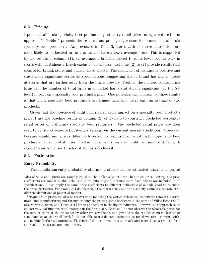
5.2 Pricing

I predict California specialty beer producers’ post-entry retail prices using a reduced-form

approach.35 Table 5 presents the results from pricing regressions for brands of California

specialty beer producers. As previewed in Table 3, stores with exclusive distributors are

more likely to be located in rural areas and have a lower average price. This is supported

by the results in column (1): on average, a brand is priced 10 cents lower per six-pack in

stores with an Anheuser Busch exclusive distributor. Columns (2) to (7) provide results that

control for brand, store, and quarter fixed effects. The coefficient of distance is positive and

statistically significant across all specifications, suggesting that a brand has higher prices

at stores that are farther away from the firm’s brewery. Neither the number of California

firms nor the number of total firms in a market has a statistically significant (at the 5%

level) impact on a specialty beer product’s price. One potential explanation for these results

is that many specialty beer producers are fringe firms that carry only an average of two

products.

Given that the presence of additional rivals has no impact on a specialty beer product’s

price, I use the baseline results in column (2) of Table 5 to construct predicted post-entry

retail prices of California specialty beer producers. The predicted retail prices are then

used to construct expected post-entry sales given the current market conditions. Moreover,

because equilibrium prices differ with respect to exclusivity, in estimating specialty beer

producers’ entry probabilities, I allow for a firm’s variable profit per unit to differ with

regard to an Anheuser Busch distributor’s exclusivity.

5.3 Estimation

Entry Probability

The equilibrium entry probability of firm i at store s can be estimated using its empirical

sales of wine and spirits are roughly equal to the dollar sales of beer. In the empirical setting, the pricecoefficients are robust to this definition of an outside good, because store fixed effects are included in allspecifications. I also apply the same price coefficients to different definitions of outside good to calculatethe price elasticities. For example, I double/triple the market size, and the elasticity estimates are robust todifferent definitions of potential market.

35Equilibrium prices can also be recovered by modeling the vertical relationships between retailers, distrib-utors, and manufacturers and through solving the pricing game backward in the spirit of Villas-Boas (2007)(see Miravete, Seim, and Thurk 2014 for an application in the liquor industry). However, this approach relieson correctly backing out retail margins in the first place. Because I do not observe the wholesale prices forthe retailer chain or the prices set by other grocery chains, and given that the retailer chain is clearly nota monopolist at the retail level, I am not able to use demand estimates to pin down retail margins with-out making further assumptions. Therefore, I do not pursue this approach and instead use a reduced-formapproach to construct predicted prices.

19

counterpart. Given the panel structure of the data, a simple frequency estimator is:

σis(ais = 1) =

∑Qq=1 aiqs

Q,

where aiqs is equal to one if firm i chooses to enter store s in quarter q. The expected number

of rivals of firm i at store s is the sum of all firms’ entry probabilities subtracted by firm i’s

own entry probability.36

Demand-Side Parameters

Recall that the estimating equation for the demand system in (1) is:

ln(sjt)− ln(s0t) = xjβ − α pjt + γAjt + (1− λ1λ2λ3) ln(sj|g) + (1− λ2λ3) ln(sg|d)

+ (1− λ3) ln(sd|b) + ξjt.

There is a potential endogeneity problem in estimating the coefficients on pjt, ln(sj|g), ln(sg|d),

and ln(sd|b), because these variables may be correlated with unobserved product quality in a

specific market, ξjt. For example, if a firm has a higher unobserved quality level in market t

and is able to price higher and earn a large market share, then the price and the λ coefficients

will be biased. To deal with this endogeneity problem, I decompose ξjt = ξj + ξt +∆ξjt, in

which ξj is the unobserved brand fixed effect, ξt is the unobserved market fixed effect, and

∆ξjt is the unobserved deviation from brand and market fixed effects. Given this, I include

brand, store, and quarter dummies in the estimation to control for ξj and ξt.

Because beer tastes better when it is fresh, and consumers usually value a product more

if it is made locally, I construct a dummy variable “locally brewed” when the brewery is

located within a 10-mile radius of a store. This helps to explain some variation in ∆ξjt.

However, unobserved promotional activities at the brand level are still a concern. Therefore,

I pursue an instrumental variable approach that requires finding instrumental variables that

are correlated with the explanatory variables, but are uncorrelated with ∆ξjt. To this end, I

instrument for pjt and ln(sj|g) using the number of brands a firm carries and the number of

rival brands in group g. The maintained identification assumption in the demand estimation

is that local demand shocks are realized after firms make their entry decisions.

For a domestic (foreign) product, I similarly use the number of rival domestic (foreign)

brands with different styles and the number of total foreign (domestic) brands in the market

36I can also estimate the entry probabilities by fitting a linear probability model. I run a regression of entrydecisions on store, quarter, and firm fixed effects. I also include firm by store interactions in the regression.The predicted entry probabilities are basically the same as the ones calculated using the simple frequencyestimator described above. However, there are predictions outside of the [0, 1] interval, and thus I do notuse results from the linear probability model.

20

to instrument for ln(sg|d) and ln(sd|b), respectively. The estimation is done using the two-

stage least squares method with standard errors clustered at the store level.

Using the demand estimates and the predicted prices, I can predict sales for each firm

at each location under any rivals’ action profile using the nested logit probability formula.

Ideally, I calculate the predicted demand conditional on each potential rivals’ action profile

and use the corresponding probabilities of rivals’ action profile to construct the expected

sales. However, given that I have 26 players in the entry game, to calculate the exact expected

sales for any firm in any market I will need 225 permutations of rivals’ action profiles. To

reduce the number of permutations, the expected sales are calculated two different ways:

first by a “naive” approach and second by simulation. The naive approach uses the exact

identity of rival firms observed in the market to calculate the expected sales. The advantage

of this approach is that it only takes one evaluation for each firm in each market. I also

conduct a simulation to approximate expected sales. Using the first-stage entry probabilities,

for each store I form draws of rivals’ action profiles, calculate the sum of predicted sales from

these draws, and divide the predicted sales by the number of draws. For each location, I use

the base quarter (January to March) to form the predicted sales for the store.

Supply-Side Parameters

As discussed in previous sections, the identification strategy of the effect of exclusive

dealing on a firm’s entry decision is to control for post-entry sales and the number of expected

rivals. It is important to note that a foreclosure effect is present when exclusive dealing raises

a firm’s fixed entry cost. However, exclusive dealing may reduce a firm’s entry probability

not only by raising its fixed entry cost, but also by lowering its average variable profit.

Regarding this, I also provide several robustness checks that allow for interaction terms

between an area’s exclusivity, expected sales, and the number of rivals.

I now discuss the assumptions used to identify the strategic effect. Let Πi(ai, s, θ) =∑a−i

πi(ai, a−i, s; θ)σ−i(a−i|s) be the deterministic part of the expected profit. It has been

shown that one is not able to identify Πi(ai, s, θ) without imposing distribution assumptions

on the stochastic shocks ϵ. Following the standard treatment for this problem, I assume

ϵ is identically and independently distributed with a Type 1 extreme value distribution.

Furthermore, I am only able to identify the deterministic part of the expected profit up to

the difference between Πi(a = 1, s, θ)−Πi(a = 0, s, θ), and so I normalize Πi(a = 0, s, θ) to

zero in order to identify Πi(a = 1, s, θ). Therefore, I assume that a firm’s payoff from staying

out of the market is zero in the model, which is similar to the outside good assumption made

in standard discrete choice models. In addition, there can be multiple equilibria in the game.

Following the literature on two-step estimation methods, the estimates are herein obtained

under the assumption that in each location, firms play the same strategy and do not switch

21

to others.

The estimating equations are a system of simultaneous equations. Bajari, Hong, Krainer,

and Nekipelov (2010) discuss that one needs exclusion restrictions to non-parametrically

identify a static game. Even though nonparametric identification is not the main purpose

of this paper, having variables that satisfy exclusion restriction conditions better explains

where the identification comes from.37 Basically, the exclusion restriction condition says one

needs to have state variables that affect rival firms’ entry probabilities, but do not enter into

a firm’s payoff directly. In this paper I use the distances between rival breweries to a store to

satisfy the exclusion restriction condition. If a firm is more likely to enter stores closer to its

brewery, which is the case in the beer industry, and the locations of rival firms’ breweries do

not enter into the firm’s profit function directly, then the distances of rival firms’ breweries

to a store can serve as exclusion restrictions.

One concern of using distances to satisfy the exclusion restriction is that the proximity

to rivals’ breweries may affect a firm’s profitability through demand. If consumers prefer to

purchase locally-brewed products, then a firm’s market share can be lower when it enters

a store closer to a rival’s brewery. To deal with this problem, I include a “locally brewed”

variable in the demand estimation to capture these effects, and the maintained assumption

will be that after controlling for demand, the distance variables of rival firms do not enter

into a firm’s profit function.

Another concern is that a firm’s choice of brewery location may not be exogenous. Out

of 26 specialty beer producers in the data, 13 of them set up their breweries around San

Francisco (i.e., located within the Bay Area counties) and Sacramento.38 Because the Bay

Area counties and Sacramento County are the two major urban areas in Northern California,

the observed clusters of breweries raise a concern about whether the exclusion restrictions

are valid.39 If firms choose their breweries’ locations based on unobserved common factors in

these areas, then the estimated strategic effect will be biased upward. I address this concern

by conducting robustness checks. I provide results that include and exclude all the stores in

the counties of the Bay Area and Sacramento County.

Standard Errors

37In the main estimating equation, each firm’s entry probability into a grocery store depends both on itsdistance from the brewery to the grocery store and its rivals’ entry probabilities. Stacking all the firms’entry decisions, I arrive at a model with a system of equations. One is unable to identify the strategic effectvariable if exclusion restrictions are not imposed.

38The Bay Area counties are: Alameda County, Contra Costa County, Marin County, Napa County, SanFrancisco County, San Mateo County, Santa Clara County, Solano County, and Sonoma County.

39The average annual median household income and the monthly gross rent in the Bay Area counties andSacramento County are $62,066 and $957, respectively, while the average annual median household incomeand the monthly gross rent in the other 20 counties are $44,704 and $703, respectively.

22

Since the estimation is done in two steps, I bootstrap the standard errors across stores by

resampling. The assumption is that after controlling for brand, quarter, and store dummies,

the error terms across stores are independent. Moreover, given that I estimate a static model

with eight quarters of data, I cluster the standard errors at the store level to control for the

likely positive correlation over time.

6 Results

I first estimate an entry model without controlling for demand or strategic effects. Table 6

shows the estimation results. Column (1) provides the baseline regression results. Column

(2) further controls for gross rent, and columns (3) and (4) provide results with squared

distances as robustness checks. All coefficients on store size, distance, and gross rent have

the expected signs: a location that has a larger selling area, is closer to a firm’s brewery, or has

lower gross rent is associated with higher entry probability. All coefficients on the Anheuser

Busch exclusive distributor indicator variable are positive, though only the coefficient in (3)

is statistically significant at the 5% level. As discussed in the previous section, the coefficient

of the exclusive variable is likely to be biased upward. In fact, column (2) presents that the

coefficient of the exclusive variable goes down once I control for gross rent. To explore more

rigorously the effect of exclusive dealing on a firm’s entry decision, I proceed by estimating

the demand for beer and the entry game with strategic interactions.

6.1 Demand Estimates

The demand system is estimated to achieve two goals. First, it provides predictions for

counterfactual post-entry sales. Second, it enables welfare analysis.

Table 7 provides demand estimation results using a logit model. Column (1) gives the

OLS regression results, and column (2) provides the results from the instrumented regression.

All specifications include brand, store, and quarter fixed effects. As can be seen in column

(2), the magnitude of the negative coefficient on price increases when prices are instrumented.

In both specifications, a consumer enjoys a product more if it is brewed locally. The implied

mean price elasticity is -7.82, suggesting that the demand is quite price elastic.40

Table 8 presents the demand estimation results using a nested logit model, with prices

instrumented in column (2). Columns (3) to (6) show the first-stage results, where the

various instruments are presented in section 5.3. In column (3), the instrument for ln sj|g,

the number of rival brands in group g, is negatively correlated to ln sj|g and is significant.

40Hellerstein (2008) estimates a model of beer demand using a random-coefficients model with data from1991 to 1994. The estimated demand for beer is also very elastic. The own elasticities of her selected beerproducts are between -5.71 to -6.37. The data used by her are monthly data and contain no specialty beerproducts.

23

The results in columns (4) and (5) are similar to those in column (3) and have the expected

signs for the instruments: as the number of the brands in other rival groups increases, the

market share of a product’s own group will decrease. In column (6), the number of brands

a firm carries in group g is associated with lower prices for its brands in group g. This

association is probably due to the fact that big domestic firms are more likely to enjoy

economies of scale and are more capable of providing products at very low prices. The first-

stage F-statistics, with standard errors clustered at the store level, are 125.16, 44.27, 25.64,

and 121.09, suggesting that the instruments are not weak.

A comparison of the first two columns in Table 8 shows that demand becomes more

elastic once prices are instrumented. As in the logit model, consumers also prefer to have

local products in both specifications. The mean own price elasticity of the nested logit

model is -8.41. Table 9 provides the percentiles of price elasticities based on the logit and

the nested logit models using the estimates in columns (2) in Table 7 and Table 8. The

nested logit model provides less elastic demand estimates across percentiles. To give a sense

of the price elasticities using the nested logit model, the average own price elasticities of

Budweiser (domestic mainstream lager) and Lost Coast Downtown Brown Ale (domestic

ale) are -5.48 and -7.91, respectively. When the price of Lost Coast Downtown Brown Ale

increases, the cross price elasticity between Budweiser and Lost Coast Downtown Brown Ale

is 0.039, and the cross price elasticity between Newcastle Brown Ale (foreign ale) and Lost

Coast Downtown Brown Ale is 0.015. The substitution pattern suggests that consumers view

domestic ale and foreign ale products as more distinct products than they view domestic ale

and domestic mainstream lager products.41

The coefficients on ln(sj|g), ln(sg|d), and ln(sd|b) represent the similarities within nests.

As McFadden (1981) shows, a nested logit model is consistent with a utility maximization

model for any values if all of the inclusive value coefficients are within the [0, 1] interval.

A negative estimate of an inclusive value indicates a violation of utility maximization. The

implied inclusive value coefficients (λ1, λ2, and λ3) in the nested logit model are 1.59, 0.53,

and 0.35, respectively.42 Given that the similarity coefficients are not jointly zero, I can

reject a simple logit model, and so I use the nested logit model as my preferred setting to

predict post-entry sales.

Table 10 presents the results that control for demand, but not strategic entry decisions.

41The average price elasticities in this example are calculated using data from stores with positive sales ofthe above three products.

42The coefficient λ1 being greater than one means consumers substitute more often across different beerstyles than within the same style. However, I cannot reject the hypothesis that λ1 is equal to one at the 5%level. I also estimate equation (1) with the constraint that λ1 is equal to one, and the results are similar tothose reported above.

24

The first two columns restrict the average variable profits of sales across firms to be the same.

Column (3) allows average variable profits of sales to differ across firms, and columns (4),

(5), and (6) add the squared distance as robustness checks. The coefficients on expected sales

have the expected positive signs and are significant. Compared to the results in Table 6, the

exclusive coefficients are smaller and are no longer statistically significant in all specifications.

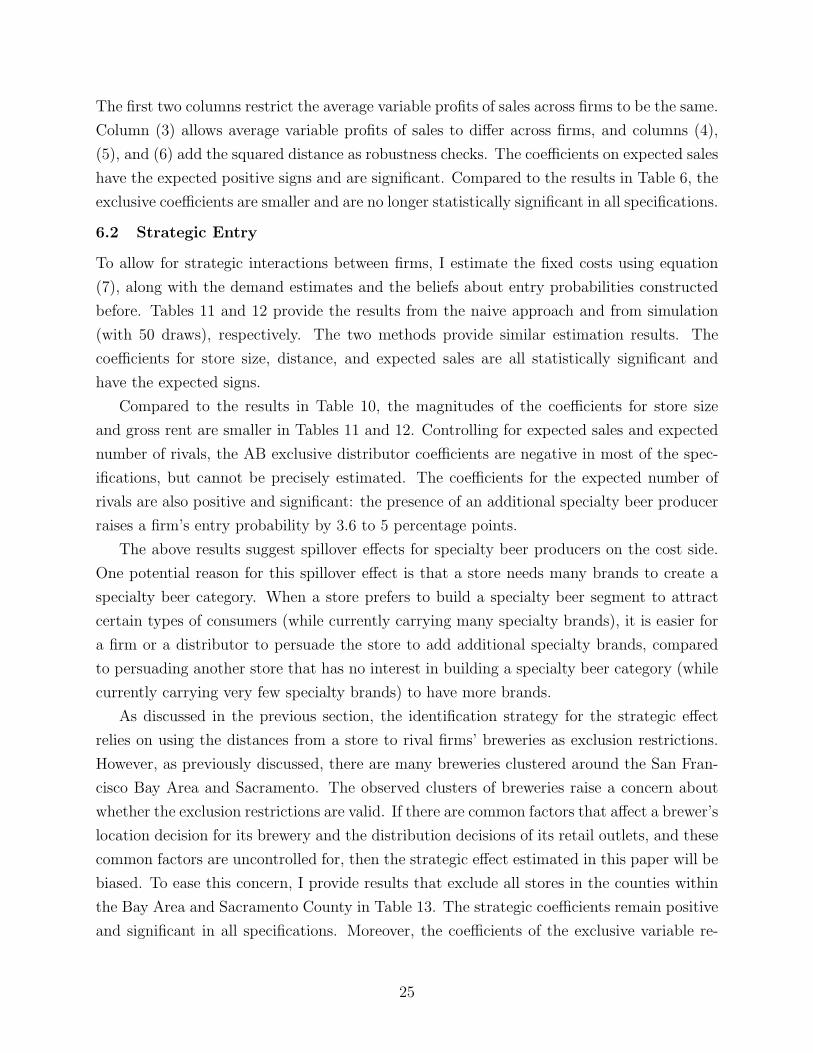
6.2 Strategic Entry

To allow for strategic interactions between firms, I estimate the fixed costs using equation

(7), along with the demand estimates and the beliefs about entry probabilities constructed

before. Tables 11 and 12 provide the results from the naive approach and from simulation

(with 50 draws), respectively. The two methods provide similar estimation results. The

coefficients for store size, distance, and expected sales are all statistically significant and

have the expected signs.

Compared to the results in Table 10, the magnitudes of the coefficients for store size

and gross rent are smaller in Tables 11 and 12. Controlling for expected sales and expected

number of rivals, the AB exclusive distributor coefficients are negative in most of the spec-

ifications, but cannot be precisely estimated. The coefficients for the expected number of

rivals are also positive and significant: the presence of an additional specialty beer producer

raises a firm’s entry probability by 3.6 to 5 percentage points.

The above results suggest spillover effects for specialty beer producers on the cost side.

One potential reason for this spillover effect is that a store needs many brands to create a

specialty beer category. When a store prefers to build a specialty beer segment to attract

certain types of consumers (while currently carrying many specialty brands), it is easier for

a firm or a distributor to persuade the store to add additional specialty brands, compared

to persuading another store that has no interest in building a specialty beer category (while

currently carrying very few specialty brands) to have more brands.

As discussed in the previous section, the identification strategy for the strategic effect

relies on using the distances from a store to rival firms’ breweries as exclusion restrictions.

However, as previously discussed, there are many breweries clustered around the San Fran-

cisco Bay Area and Sacramento. The observed clusters of breweries raise a concern about

whether the exclusion restrictions are valid. If there are common factors that affect a brewer’s

location decision for its brewery and the distribution decisions of its retail outlets, and these

common factors are uncontrolled for, then the strategic effect estimated in this paper will be

biased. To ease this concern, I provide results that exclude all stores in the counties within

the Bay Area and Sacramento County in Table 13. The strategic coefficients remain positive

and significant in all specifications. Moreover, the coefficients of the exclusive variable re-

25

main negative, but are now statistically significant in all specifications, suggesting that there

is a foreclosure effect due to Anheuser Busch’s exclusive dealing program in areas where

microbreweries are not clustered. The coefficients of “store size” are greatly reduced in all

specifications and are not precisely estimated, probably because the stores in the subsample

are more likely to be located in rural areas where the size of the physical selling area is less

likely to play a major role in affecting a product’s shelf availability.

To interpret the magnitude of the foreclosure effect in potentially foreclosed areas, I use

the estimates from column (2) in Table 13 to calculate the marginal effects. I find that a

store with an Anheuser Busch exclusive distributor reduces a firm’s entry probability by

approximately 6 percentage points. The effect does not appear large at first glance, but

given that the mean entry probability of the 23 specialty beer producers in the subsample

is only 28 percentage points (excluding the three California firms that enter all 229 stores),

the exclusive effect plays an important role in a firm’s entry decisions. The results also

show that a decrease in sales of 100 six-packs a quarter reduces a firm’s entry probability

by 6 percentage points, a reduction in 10,000 square feet of store size reduces a firm’s entry

probability by 1 percentage point, and a 10-mile increase in the distance between a firm’s

brewery and a store reduces the firm’s entry probability by 3.4 percentage points.

I finally conduct counterfactual experiments to study the effect of banning exclusive

dealing through relaxing the foreclosure effect on consumer welfare and Anheuser Busch’s

sales. Holding equilibrium prices constant, in areas where exclusive dealing is banned, the

entry probabilities of specialty beer producers increase. In such situations, consumers are

able to select beer products from a presumed more diverse mix, and the magnitude of the

increase in consumer welfare would depend on the product attributes of the newly included

products. The monetary measure that is used here is equivalent variation, which measures

the income changes required to make consumers just as well off as they are once their choice

sets are expanded.

I simulate demand using the predicted entry probabilities with and without exclusive

dealing. Following Small and Rosen (1981), the changes in consumer welfare per consumer

per quarter can be found by:

∆EVt =1

α

[ln(∑

j∈J1

eδj)− ln

(∑j∈J0

eδj)]

,

where J0 and J1 are the respective choice sets before and after removing exclusive dealing.43

Table 14 provides the results of counterfactual experiments based on 100 draws from

43I find∑j∈J

eδj by using the(1 + exp(dqzq + dtzt + λ3I3)

)term in equation (3).

26

the predicted entry probabilities. Removing exclusive dealing does not have much impact

on entry behavior: at most only one additional firm will enter a market, and the impact

on consumer welfare is almost zero. The average quarterly sales per store in an exclusive

dealing area are less than 30,000 six-packs, and with an average welfare increase of $0.0005

per quarter per six-pack, changes in consumer welfare per store per quarter are less than

$15. In fact, given the demand structure, even if we allow all the California specialty beer

producers to enter a store with an Anheuser Busch exclusive distributor, the implied increase

in an average consumer’s welfare is around $0.017 per market (a store in a quarter).

There are several reasons for getting such small estimates. First, as shown in Table 5,

adding specialty brands does not impact pricing very much. Second, most of the specialty

brands that do not have a presence in many markets have very little market shares even

in stores where they do have a presence. It is also important to note that the welfare im-

provement from adding more products may be even less than the above estimates. This is

because in the demand model employed in this paper, each new product enters by adding

independent and identically distributed logit errors, which allows consumers’ willingness to

pay for new products to increase without bound as the number of products increases. There-

fore, though exclusive dealing increases the fixed costs for some specialty beer producers,

the welfare improvement from banning exclusive dealing is very limited. Moreover, as dis-

cussed throughout the paper, exclusive contracts may lead to efficiency gains that eventually

enhance consumer welfare, and thus banning such contracts may involve a decrease in con-

sumer welfare. Consequently, the estimate from removing exclusive dealing reported above

reflects an upper bound on the net benefits associated with banning exclusive dealing.

The results in Table 14 also imply that foreclosure alone is not the motivation behind

Anheuser Busch’s continuous support for its exclusive program. Enforcing exclusive dealing

may decrease the entry probability of specialty beer producers, yet the market shares of

these potentially foreclosed firms are extremely low to begin with. The demand substitution

pattern of beer products also restricts the gains of Anheuser Busch from profiting through

foreclosure: the increase in diverted sales from foreclosing one additional specialty beer pro-

ducer is at most 31 six-packs per store per quarter. Therefore, while the empirical evidence

suggests that in some rural markets exclusive dealing may lower rivals’ entry probability, the

effect is more likely a side-effect of Anheuser Busch’s exclusive dealing program.

6.3 Robustness Checks

One potential concern about the preferred specification is that even if exclusive dealing

reduces the entry probability of specialty beer producers, it may not be driven by higher fixed

distribution costs. There are two ways to interpret the correlation between the reduction of

27

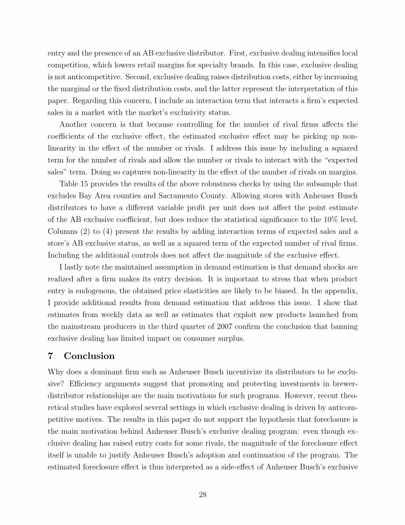
entry and the presence of an AB exclusive distributor. First, exclusive dealing intensifies local

competition, which lowers retail margins for specialty brands. In this case, exclusive dealing

is not anticompetitive. Second, exclusive dealing raises distribution costs, either by increasing

the marginal or the fixed distribution costs, and the latter represent the interpretation of this

paper. Regarding this concern, I include an interaction term that interacts a firm’s expected

sales in a market with the market’s exclusivity status.

Another concern is that because controlling for the number of rival firms affects the

coefficients of the exclusive effect, the estimated exclusive effect may be picking up non-

linearity in the effect of the number or rivals. I address this issue by including a squared

term for the number of rivals and allow the number or rivals to interact with the “expected

sales” term. Doing so captures non-linearity in the effect of the number of rivals on margins.

Table 15 provides the results of the above robustness checks by using the subsample that

excludes Bay Area counties and Sacramento County. Allowing stores with Anheuser Busch

distributors to have a different variable profit per unit does not affect the point estimate

of the AB exclusive coefficient, but does reduce the statistical significance to the 10% level.

Columns (2) to (4) present the results by adding interaction terms of expected sales and a

store’s AB exclusive status, as well as a squared term of the expected number of rival firms.

Including the additional controls does not affect the magnitude of the exclusive effect.

I lastly note the maintained assumption in demand estimation is that demand shocks are

realized after a firm makes its entry decision. It is important to stress that when product

entry is endogenous, the obtained price elasticities are likely to be biased. In the appendix,

I provide additional results from demand estimation that address this issue. I show that

estimates from weekly data as well as estimates that exploit new products launched from

the mainstream producers in the third quarter of 2007 confirm the conclusion that banning

exclusive dealing has limited impact on consumer surplus.

7 Conclusion

Why does a dominant firm such as Anheuser Busch incentivize its distributors to be exclu-

sive? Efficiency arguments suggest that promoting and protecting investments in brewer-

distributor relationships are the main motivations for such programs. However, recent theo-

retical studies have explored several settings in which exclusive dealing is driven by anticom-

petitive motives. The results in this paper do not support the hypothesis that foreclosure is

the main motivation behind Anheuser Busch’s exclusive dealing program: even though ex-

clusive dealing has raised entry costs for some rivals, the magnitude of the foreclosure effect

itself is unable to justify Anheuser Busch’s adoption and continuation of the program. The

estimated foreclosure effect is thus interpreted as a side-effect of Anheuser Busch’s exclusive

28

dealing program. In addition, the estimated change in consumer welfare when exclusive

dealing is removed is very limited. The results, along with recent studies from Sass (2005),

Rojas (2010), and Chen (2013), suggest that exclusive dealing in the beer industry is un-

likely a device used by Anheuser Busch solely to foreclose new entrants or to dampen market

competition, but is more likely a mechanism to compete with other brewers more efficiently.

It should be noted that the results of this paper refer to data used from one major grocery

chain in Northern California. On the one hand, because grocery stores are only one of many

retail channels for beer products, if the entry of specialty beer products is not depressed in

other retail formats, then the overall foreclosure effect might not even harm specialty beer

producers as much. On the other hand, because all results are based on data of Northern

California, in which consumers historically have more appeal to specialty beer products, the

foreclosure effect may be larger in other states.

One limitation of this paper is that the welfare analysis herein focuses only on consumer

surplus from direct beer consumption and does not include potential (negative) externalities

caused by beer consumption. The negative externalities from alcohol consumption are some

of the reasons for regulations in the beer industry. However, a comprehensive welfare analysis

for the societal effects of beer consumption is beyond the scope of this paper.

Entry decisions of firms are jointly determined by many factors. In this paper I find that

a dominant incumbent’s vertical arrangements with its existing distributors have raised the

fixed costs of specialty beer producers significantly in some areas. The presence of other

specialty beer producers, to the contrary, results in a spillover effect and lowers the fixed

costs of specialty beer producers. Given the static setting in this paper, it is difficult to

disentangle whether the above effects come from changes in sunk costs or in fixed costs

in every period. Future research on questions regarding entry and market structure in a

dynamic setting will be highly valuable.

29

References

Abito, J. M., Wright, J., 2008. Exclusive dealing with imperfect downstream competition.

International Journal of Industrial Organization 26 (1), 227–246.

Aghion, P., Bolton, P., 1987. Contracts as a barrier to entry. American Economic Review

77 (3), 388–401.

Aguirregabiria, V., Mira, P., 2002. Swapping the nested fixed point algorithm: A class of

estimators for discrete markov decision models. Econometrica 70 (4), 1519–1543.

Asker, J., 2005. Diagnosing foreclosure due to exclusive dealing, working paper, Stern School

of Business, New York University.

Asker, J., Bar-Isaac, H., 2014. Raising retailers’ profits: On vertical practices and the exclu-

sion of rivals. American Economic Review 104 (2), 672–86.

Augereau, A., Greenstein, S., Rysman, M., 2006. Coordination versus differentiation in a

standards war: 56k modems. RAND Journal of Economics 37 (4), 887–909.

Bajari, P., Benkard, C. L., Levin, J., 2007. Estimating dynamic models of imperfect compe-

tition. Econometrica 75 (5), 1331–1370.

Bajari, P., Hong, H., Krainer, J., Nekipelov, D., 2010. Estimating static models of strategic

interactions. Journal of Business and Economic Statistics 28 (4), 469–482.

Bernheim, B. D., Whinston, M. D., 1998. Exclusive dealing. Journal of Political Economy

106 (1), 64–103.

Berry, S. T., 1992. Estimation of a model of entry in the airline industry. Econometrica

60 (4), 889–917.

Berry, S. T., 1994. Estimating discrete-choice models of product differentiation. RAND Jour-

nal of Economics 25 (2), 242–262.

Besanko, D., Perry, M. K., 1993. Equilibrium incentives for exclusive dealing in a differenti-

ated products oligopoly. RAND Journal of Economics 24 (4), 646–667.

Bork, R. H., 1978. The Antitrust Paradox: A Policy at War with Itself. Basic Books.

Bresnahan, T. F., Reiss, P. C., 1991. Entry and competition in concentrated markets. Journal

of Political Economy 99 (5), 977–1009.

30

Bronnenberg, B. J., Dhar, S. K., Dube, J.-P. H., 2009. Brand history, geography, and the

persistence of brand shares. Journal of Political Economy 117 (1), 87–115.

Cardell, N. S., 1997. Variance components structures for the extreme-value and logistic

distributions with application to models of heterogeneity. Econometric Theory 13 (2),

185–213.

Chen, C.-W., 2013. Does exclusive dealing matter? Evidence from distribution contract

changes in the U.S. beer industry, working paper, Department of Economics, National

Taipei University.

Chiou, L., 2008. The timing of movie releases: Evidence from the home video industry.

International Journal of Industrial Organization 26 (5), 1059–1073.

Conlon, C. T., Mortimer, J. H., 2013. Efficiency and foreclosure effects of all-units discounts:

Empirical evidence, NBER working paper.

Conlon, C. T., Rao, N. S., 2014. The price of liquor is too damn high: State facilitated

collusion and the implications for taxes, working paper.

Crawford, G. S., Yurukoglu, A., 2012. The welfare effects of bundling in multichannel tele-

vision markets. American Economic Review 102 (2), 643–85.

Dick, A. A., 2008. Demand estimation and consumer welfare in the banking industry. Journal

of Banking & Finance 32 (8), 1661–1676.

Doganoglu, T., Wright, J., 2010. Exclusive dealing with network effects. International Journal

of Industrial Organization 28 (2), 145–154.

Einav, L., 2007. Seasonality in the U.S. motion picture industry. RAND Journal of Economics

38 (1), 127–145.

Eizenberg, A., 2014. Upstream innovation and product variety in the U.S. home PC market.

The Review of Economic Studies.

Ellickson, P. B., Misra, S., 2008. Supermarket pricing strategies. Marketing Science 27 (5),

811–828.

Goldberg, P. K., 1995. Product differentiation and oligopoly in international markets: The

case of the U.S. automobile industry. Econometrica 63 (4), 891–951.

Hellerstein, R., 2008. Who bears the cost of a change in the exchange rate? Pass-through

accounting for the case of beer. Journal of International Economics 76 (1), 14–32.

31

Hendel, I., Nevo, A., 2006. Sales and consumer inventory. The RAND Journal of Economics

37 (3), pp. 543–561.

Ho, K., Ho, J., Mortimer, J. H., 2012. The use of full-line forcing contracts in the video

rental industry. American Economic Review 102 (2), 686–719.

Kesmodel, D., 2007. To trump small brewers, beer makers get crafty. Wall Street Journal -

Eastern Edition 250 (99), B1–B3.

Klein, B., Murphy, K. M., 1988. Vertical restraints as contract enforcement mechanisms.

Journal of Law and Economics 31 (2), 265–297.

Lafontaine, F., Slade, M. E., 2007. Vertical integration and firm boundaries: The evidence.

Journal of Economic Literature 45 (3), 629–685.

Lafontaine, F., Slade, M. E., 2008. Exclusive contracts and vertical restraints: Empirical

evidence and public policy. In: Buccirossi, P. (Ed.), Handbook of Antitrust Economics.

MIT Press, pp. 391–414.

Lee, R. S., 2013. Vertical integration and exclusivity in platform and two-sided markets.

American Economic Review 103 (7), 2960–3000.

Martimort, D., 1996. Exclusive dealing, common agency, and multiprincipals incentive the-

ory. RAND Journal of Economics 27 (1), 1–31.

Marvel, H. P., 1982. Exclusive dealing. Journal of Law and Economics 25 (1), 1–25.

McFadden, D. L., 1978. Modeling the choice of residential location. In: Karlqvist, A.,

Lundqvist, L., Snickers, F., Weinull, J. (Eds.), Spatial Interaction Theory and Planning

Models. North-Holland.

Miravete, E., Seim, K., Thurk, J., 2014. Complexity, efficiency, and fairness of multi-product

monopoly pricing, working paper.

Musalem, A., Shin, W., 2013. When demand projections are too optimistic: A structural

model of product line and pricing decisions, working paper.

Nevo, A., 2000. A practitioner’s guide to estimation of random-coefficients logit models of

demand. Journal of Economics & Management Strategy 9 (4), 513–548.

Pakes, A., Ostrovsky, M., Berry, S., 2007. Simple estimators for the parameters of discrete

dynamic games (with entry/exit examples). RAND Journal of Economics 38 (2), 373–399.

32

Posner, R. A., 1976. Antitrust Law: An Economic Perspective. University of Chicago Press.

Rasmusen, E. B., Ramseyer, J. M., Wiley, J. S. J., 1991. Naked exclusion. American Eco-

nomic Review 81 (5), 1137–1145.

Rojas, C., 2010. The competitive and welfare effects of exclusive agreements: Evidence

from US brewing, working paper, Department of Resource Economics, University of Mas-

sachusetts at Amherst.

Rust, J., 1987. Optimal replacement of GMC bus engines: An empirical model of Harold

Zurcher. Econometrica 55 (5), 999–1033.

Salop, S. C., Scheffman, D. T., 1983. Raising rivals’ costs. American Economic Review 73 (2),

267–271.

Sass, T. R., 2005. The competitive effects of exclusive dealing: Evidence from the U.S. beer

industry. International Journal of Industrial Organization 23 (3-4), 203–225.

Segal, I. R., Whinston, M. D., 2000a. Exclusive contracts and protection of investments.

RAND Journal of Economics 31 (4), 603–633.

Segal, I. R., Whinston, M. D., 2000b. Naked exclusion: Comment. American Economic

Review 90 (1), 296–309.

Seim, K., 2006. An empirical model of firm entry with endogenous product-type choices.

RAND Journal of Economics 37 (3), 619–640.

Seim, K., Waldfogel, J., 2013. Public monopoly and economic efficiency: Evidence from

the Pennsylvania liquor control board’s entry decisions. The American Economic Review

103 (2), pp. 831–862.

Simpson, J., Wickelgren, A. L., 2007. Naked exclusion, efficient breach, and downstream

competition. American Economic Review 97 (4), 1305–1320.

Sinkinson, M., 2014. Pricing and entry incentives with exclusive contracts: Evidence from

smartphones, working paper, Business Economics and Public Policy Department, The

Wharton School at the University of Pennsylvania.

Small, K. A., Rosen, H. S., 1981. Applied welfare economics with discrete choice models.

Econometrica 49 (1), 105–130.

Sweeting, A., 2009. The strategic timing incentives of commercial radio stations: An empir-

ical analysis using multiple equilibria. RAND Journal of Economics 40 (4), 710–742.

33

Tremblay, V. J., Tremblay, C. H., 2005. The U.S. Brewing Industry: Data and Economic

Analysis. MIT Press.

Villas-Boas, S. B., 2007. Vertical relationships between manufacturers and retailers: Infer-

ence with limited data. The Review of Economic Studies 74 (2), pp. 625–652.

Vitorino, M. A., 2012. Empirical entry games with complementarities: An application to the

shopping center industry. Journal of Marketing Research 49 (2), 175–191.

34

Table 1: Some Typical Entries From the CBBD Annual Directory

Distribution Status Brand Portfolio

Exclusive AB distributor 180 Energy Drink, Anheuser-Busch, Redhook Ale Brewery,Rolling Rock, Widmer Brothers Brewing

Non-exclusive AB distributor Anheuser Busch, Arizona Beverage, Gambrinus, GordonBiersch Brewing, Heineken USA, InBev USA, RedhookAle Brewery, Scottish & Newcastle Importers, Sierra NevadaBrewing, Spaten North America, Widmer Brothers Brewing

Non-AB distributor 1 Anchor Brewing, Asahi Breweries, Boston Beer,Diageo-Guinness USA, Gambrinus, Heineken, Hornell Brewing,InBev USA, Mark Anthony Brands, McKenzie River,Miller Brewing, Pabst Brewing, Pyramid Breweries, Sapporo USA,Scottish & Newcastle Importers, Sierra Nevada Brewing,Sierra Springs Water, US Beverage

Non-AB distributor 2 Alaskan Brewing, Barton Beers, Boston Beer, Diageo-GuinnessUSA, InBev USA, Lake Tahoe Brewing, Mark Anthony Brands,Miller Brewing, Molson Coors Brewing, New Belgium Brewing,Pyramid Breweries, Redhook Ale Brewery, Sapporo USA,Sierra Nevada Brewing

Independent distributor Alaskan Brewing, Allagash Brewing, Anderson Valley Brewing,Arizona Beverage, Asahi Breweries USA, Bear Republic,Binding International, Bison Brewing, California Cider,Constancia Brewery, Firestone-Walker Brewing, Friedlin ImportsFull Sail Brewing Co., Humboldt Brewing, InBev USA,Mad River Brewing, Mendocino Brewing, Marin Brewing,Moylan’s Brewery, Nestle Beverage, Ommegang Brewery,Pabst Brewing, Panorama Brewing, Sapporo USA,Scottish & Newcastle Importers, Sierra Nevada Brewing,Spaten North America, Speakeasy, Stone Brewing, SudwerkPrivatbrauerei, Thames America Trading, US Beverage,Wyder’s Beverage

Notes: AB (Anheuser Busch). 180 Energy Drink, Redhook, Rolling Rock, and Widmer Brothers are all affiliated AnheuserBusch products listed on the Anheuser Busch company website. California specialty beer producers that can be matched tothe scanner dataset are denoted by bold type.

Table 2: Number of Entrants and the Minimum Six-Packs Sold During a Quarter per Store

Top 10 stores with the Bottom 10 stores with themost number of CA least number of CA

specialty beer producers specialty beer producers

Number of CA firms 12.3 5.4

Minimum six-packs sold per quarter 15.4 43.4

Average price 7.16 7.31

Note: Average price (in $) is the price of products from California specialty beer producers.

35

Table 3: Summary Statistics

Anheuser Busch Anheuser BuschNon-exclusive Stores Exclusive Stores

Number of stores 189 40

Number of CA specialty beer producers 9.29 10.06(1.61) (1.19)

Store total sales 24362 29148(9025.83) (8835.98)

Store size 2.87 3.07(1.09) (0.90)

Population 33255 26236(16740) (12966)

Household income 64964 48375(22403) (18137)

Gross rent 992 794(278) (254)

Notes: All entries reported are means with standard deviations shown in parentheses. “Store total sales” are thenumber of volume-adjusted six-packs (in quantity) sold per quarter. “Store size” is measured in 10,000 square feet.

Table 4: Number of Stores a Firm Entered

Firm 2006q2 2006q3 2006q4 2007q1 2007q2 2007q3 2007q4 2008q1 mean

Non-CA Firm 1 204 204 203 204 203 209 211 210 206Non-CA Firm 2 229 229 229 229 229 229 229 229 229Non-CA Firm 3 188 193 192 197 197 210 209 205 199Non-CA Firm 4 193 193 191 193 194 200 197 197 195Non-CA Firm 5 215 217 214 213 209 216 152 143 197Non-CA Firm 6 229 229 229 229 229 229 229 229 229CA Firm 1 229 229 229 229 229 229 229 229 229CA Firm 2 174 172 168 166 164 177 165 161 168CA Firm 3 126 114 111 110 109 150 152 149 128CA Firm 4 6 6 6 7 7 7 5 8 7CA Firm 5 3 97 177 20 6 4 1 0 39CA Firm 6 3 3 3 3 3 3 2 2 3CA Firm 7 4 4 4 4 4 4 4 4 4CA Firm 8 2 2 2 2 2 2 2 2 2CA Firm 9 11 3 1 0 1 0 0 0 2CA Firm 10 193 196 198 200 198 207 202 200 199CA Firm 11 229 229 229 229 229 229 229 229 229CA Firm 12 3 3 3 3 3 4 5 4 4CA Firm 13 220 221 221 222 223 229 229 229 224CA Firm 14 3 3 3 3 3 3 3 2 3CA Firm 15 181 175 172 173 172 177 199 203 182CA Firm 16 9 8 8 8 9 8 8 8 8CA Firm 17 1 1 1 1 1 1 1 1 1CA Firm 18 209 212 216 220 219 221 215 215 216CA Firm 19 3 2 2 2 2 2 0 0 2CA Firm 20 47 42 36 38 38 32 16 12 33CA Firm 21 1 1 1 1 1 0 0 0 1CA Firm 22 227 225 225 225 225 229 229 229 227CA Firm 23 6 7 8 7 8 17 6 2 8CA Firm 24 229 229 229 229 229 229 229 229 229CA Firm 25 9 9 9 9 8 8 7 7 8CA Firm 26 7 7 7 6 6 6 1 1 5Total 106 108 110 106 105 108 105 104 107

Notes: All entries reported are the counts of the variable “enter” for a firm across stores during a quarter. Thevariable “enter” is equal to one if a firm has positive sales in a store during a quarter.

36

Table 5: Pricing for California Specialty Beer Products

(1) (2) (3) (4) (5) (6) (7)Distance 0.062∗ 0.081∗ 0.082∗ 0.082∗ 0.295∗∗ 0.295∗∗ 0.295∗∗

(0.024) (0.035) (0.035) (0.035) (0.102) (0.102) (0.102)

AB exclusive distributor -0.104∗∗

(0.028)

Number of CA micro firms -0.004 -0.004(0.004) (0.004)

Number of firms -0.003 -0.003(0.002) (0.002)

Distance2 -0.097∗∗ -0.097∗∗ -0.097∗∗

(0.033) (0.033) (0.033)

Constant 7.871∗∗ 7.888∗∗ 7.913∗∗ 7.967∗∗ 7.822∗∗ 7.846∗∗ 7.900∗∗

(0.040) (0.065) (0.073) (0.086) (0.048) (0.058) (0.073)

Store fixed effects? No Yes Yes Yes Yes Yes YesObservations 41027 41027 41027 41027 41027 41027 41027Adjusted R2 0.874 0.880 0.880 0.880 0.881 0.881 0.881

Notes: “Distance” is measured in hundreds of miles. All prices are volume adjusted six-pack prices. Data are collapsed to quar-ter/store/brand level. All regressions control for brand and quarter fixed effects. Standard errors, clustered at the store level, are shownin parentheses.+ significant at 10%, ∗ significant at 5%, ∗∗ significant at 1%.

37

Table 6: Entry Probability without Controlling for Demand

(1) (2) (3) (4)

AB exclusive distributor 0.263 0.197 0.369∗ 0.299+

(0.168) (0.181) (0.172) (0.181)

Store size 0.455∗∗ 0.448∗∗ 0.460∗∗ 0.453∗∗

(0.101) (0.100) (0.101) (0.101)

Distance -1.850∗∗ -1.866∗∗ -3.185∗∗ -3.218∗∗

(0.163) (0.161) (0.356) (0.358)

Gross rent -0.035 -0.038(0.028) (0.028)

Distance2 0.540∗∗ 0.549∗∗

(0.135) (0.138)

Constant -4.167∗∗ -3.802∗∗ -3.703∗∗ -3.312∗∗

(0.529) (0.628) (0.555) (0.654)

Observations 42136 42136 42136 42136Log likelihood -7473.200 -7463.841 -7413.057 -7401.972

Notes: Data are collapsed to quarter/store/firm level. Results are Logit regression estimates wherethe dependent variable is California specialty beer producers’ actual entry decision. All regressionscontrol for firm fixed effects. Standard errors, clustered at the store level, are shown in parentheses.AB (Anheuser Busch). “Distance” is measured in hundreds of miles. “Store size” is measured in 10,000square feet. “Gross rent” is measured in hundreds of dollars.+ significant at 10%, ∗ significant at 5%, ∗∗ significant at 1%.

Table 7: Demand Estimation Results from the Logit Model

(1) (2)OLS 2SLS

Locally brewed 0.643∗∗ 0.527∗∗

(0.056) (0.053)

Price -0.319∗∗ -1.538∗∗

(0.009) (0.177)

Constant -4.192∗∗ 7.148∗∗

(0.200) (1.644)Observations 205467 205467Adjusted R2 0.805 0.687

Notes: Data are collapsed to quarter/store/brand level. All regressions control for brand,quarter, and store fixed effects. Standard errors, clustered at the store level, are shownin parentheses. “Locally brewed” is equal to one when a store is located within a 10-mileradius of a firm’s brewery.+ significant at 10%, ∗ significant at 5%, ∗∗ significant at 1%.

38

Table 8: Demand Estimation Results from the Nested Logit Model

First-stage results

OLS 2SLS ln(sj|g) ln(sg|d) ln(sd|b) Price

(1) (2) (3) (4) (5) (6)

Locally brewed 0.002∗ 0.141+ 0.503∗∗ 0.196∗∗ -0.040∗∗ -0.087(0.001) (0.083) (0.061) (0.024) (0.009) (0.054)

Price 0.000 -0.353(0.001) (0.238)

ln(sj|g) 0.998∗∗ 0.704∗∗(0.000) (0.173)

ln(sg|d) 0.996∗∗ 0.814∗∗(0.001) (0.118)

ln(sd|b) 1.000∗∗ 0.649∗∗(0.001) (0.241)

Instrumental variables for:

Price 0.034∗∗ 0.027∗∗ 0.006∗∗ -0.048∗∗(0.008) (0.006) (0.002) (0.004)

ln(sj|g) -0.022∗∗ 0.024∗∗ 0.004∗∗ -0.002∗∗(0.002) (0.004) (0.001) (0.001)

ln(sg|d) -0.002∗∗ -0.004∗∗ 0.003∗∗ -0.002∗∗(0.001) (0.001) (0.001) (0.000)

ln(sd|b) -0.003∗∗ -0.003∗∗ -0.005∗∗ 0.005∗∗(0.001) (0.001) (0.001) (0.000)

Constant -0.779∗∗ 1.001 -2.293∗∗ -3.443∗∗ -0.376∗∗ 9.392∗∗(0.014) (1.343) (0.199) (0.030) (0.024) (0.121)

Observations 205467 205467 205467 205467 205467 205467First-stage F-statistics 125.16 44.27 25.64 121.09Adjusted R2 0.996 0.975 0.852 0.937 0.914 0.936

Notes: Data are collapsed to quarter/store/brand level. All regressions control for brand, quarter, and store fixed effects.Standard errors, clustered at the store level, are shown in parentheses. “Locally brewed” is equal to one when a store islocated within a 10-mile radius of a firm’s brewery.+ significant at 10%, ∗ significant at 5%, ∗∗ significant at 1%.

Table 9: Price Elasticity Percentiles

10% 25% median 75% 90%

Logit -12.27 -11.31 -9.75 -7.07 -5.95

Nested logit -10.64 -9.45 -7.81 -6.05 -4.69

Notes: Price elasticities are calculated using columns (2) in Table 7 and Table 8.

39

Table 10: Entry Probability with Expected Demand: No Strategic Interactions

(1) (2) (3) (4) (5) (6)

AB exclusive distributor 0.084 0.036 -0.018 0.197 0.144 0.075(0.163) (0.180) (0.179) (0.165) (0.179) (0.177)

Store size 0.383∗∗ 0.378∗∗ 0.332∗∗ 0.386∗∗ 0.381∗∗ 0.333∗∗

(0.092) (0.092) (0.091) (0.093) (0.092) (0.091)

Distance -1.743∗∗ -1.756∗∗ -1.717∗∗ -3.135∗∗ -3.158∗∗ -2.808∗∗

(0.162) (0.160) (0.158) (0.357) (0.358) (0.353)

Expected sales 0.007∗∗ 0.007∗∗ 0.007∗∗ 0.007∗∗

(0.001) (0.001) (0.001) (0.001)

Gross rent -0.026 -0.015 -0.029 -0.018(0.027) (0.028) (0.027) (0.028)

Distance2 0.563∗∗ 0.568∗∗ 0.440∗∗

(0.131) (0.132) (0.133)

Constant -4.133∗∗ -3.859∗∗ -6.243∗∗ -3.644∗∗ -3.347∗∗ -5.797∗∗

(0.505) (0.608) (0.750) (0.531) (0.632) (0.788)

Margins vary by firm? No No Yes No No Yes

Observations 42136 42136 42136 42136 42136 42136Log likelihood -7328.432 -7323.275 -6945.453 -7265.361 -7259.052 -6908.656

Notes: Data are collapsed to quarter/store/firm level. All regressions control for firm fixed effects. Standard errors, clustered at thestore level, are shown in parentheses. AB (Anheuser Busch). “Distance” is measured in hundreds of miles. “Store size” is measured in10,000 square feet. “Gross rent” is measured in hundreds of dollars.+ significant at 10%, ∗ significant at 5%, ∗∗ significant at 1%.

40

Table 11: Strategic Entry: the Naive Approach

(1) (2) (3) (4) (5) (6)

AB exclusive distributor -0.092 -0.130 -0.163 0.038 -0.005 -0.045(0.087) (0.096) (0.111) (0.091) (0.096) (0.108)

Store size 0.187∗∗ 0.183∗∗ 0.153∗∗ 0.187∗∗ 0.183∗∗ 0.149∗∗

(0.052) (0.051) (0.055) (0.050) (0.050) (0.052)

Distance -1.792∗∗ -1.802∗∗ -1.748∗∗ -3.325∗∗ -3.339∗∗ -3.071∗∗

(0.148) (0.147) (0.143) (0.349) (0.344) (0.362)

Expected sales 0.004∗∗ 0.004∗∗ 0.004∗∗ 0.004∗∗

(0.001) (0.001) (0.001) (0.001)

Expected number of rivals 0.623∗∗ 0.621∗∗ 0.591∗∗ 0.631∗∗ 0.630∗∗ 0.602∗∗

(0.059) (0.058) (0.061) (0.057) (0.056) (0.059)

Gross rent -0.021 -0.010 -0.024+ -0.015(0.015) (0.017) (0.015) (0.016)

Distance2 0.619∗∗ 0.621∗∗ 0.535∗∗

(0.108) (0.106) (0.117)

Constant -7.664∗∗ -7.433∗∗ -9.709∗∗ -7.164∗∗ -6.902∗∗ -9.227∗∗

(0.612) (0.621) (0.847) (0.618) (0.626) (0.855)

Margins vary by firm? No No Yes No No Yes

Observations 42136 42136 42136 42136 42136 42136Log likelihood -6799.318 -6796.272 -6487.496 -6724.039 -6719.892 -6436.687

Notes: Data are collapsed to quarter/store/firm level. All regressions control for firm fixed effects. Standard errors, clustered at the storelevel, are shown in parentheses. AB (Anheuser Busch). “Distance” is measured in hundreds of miles. “Store size” is measured in 10,000square feet. “Gross rent” is measured in hundreds of dollars.+ significant at 10%, ∗ significant at 5%, ∗∗ significant at 1%.

41

Table 12: Strategic Entry with Simulated Expected Demand

(1) (2) (3) (4) (5) (6)

AB exclusive distributor -0.088 -0.127 -0.132 0.043 -0.001 -0.018(0.088) (0.097) (0.110) (0.092) (0.096) (0.107)

Store size 0.187∗∗ 0.182∗∗ 0.150∗∗ 0.187∗∗ 0.182∗∗ 0.146∗∗

(0.052) (0.051) (0.054) (0.050) (0.050) (0.052)

Distance -1.787∗∗ -1.798∗∗ -1.713∗∗ -3.313∗∗ -3.328∗∗ -2.998∗∗

(0.148) (0.147) (0.142) (0.350) (0.345) (0.363)

Expected sales 0.004∗∗ 0.004∗∗ 0.004∗∗ 0.004∗∗

(0.001) (0.001) (0.001) (0.001)

Expected number of rivals 0.619∗∗ 0.618∗∗ 0.586∗∗ 0.629∗∗ 0.627∗∗ 0.597∗∗

(0.059) (0.058) (0.061) (0.057) (0.056) (0.059)

Gross rent -0.021 -0.011 -0.025+ -0.015(0.015) (0.017) (0.015) (0.016)

Distance2 0.616∗∗ 0.618∗∗ 0.519∗∗

(0.108) (0.107) (0.118)

Constant -7.637∗∗ -7.404∗∗ -10.002∗∗ -7.143∗∗ -6.879∗∗ -9.537∗∗

(0.612) (0.622) (0.879) (0.618) (0.627) (0.887)

Margins vary by firm? No No Yes No No Yes

Observations 42136 42136 42136 42136 42136 42136Log likelihood -6799.428 -6796.319 -6481.154 -6725.016 -6720.792 -6433.763

Notes: Expected sales are calculated by taking 50 draws of rivals’ action profile in a given market. Data are collapsed to quarter/store/firmlevel. All regressions control for firm fixed effects. Standard errors, clustered at the store level, are shown in parentheses. AB (AnheuserBusch). “Distance” is measured in hundreds of miles. “Store size” is measured in 10,000 square feet. “Gross rent” is measured in hundredsof dollars.+ significant at 10%, ∗ significant at 5%, ∗∗ significant at 1%.

42

Table 13: Strategic Entry: Regression without the Bay Area Counties and Sacramento County

(1) (2) (3) (4) (5) (6) (7)

AB exclusive distributor -0.297 -0.388∗ -0.458∗ -0.479∗ -0.262+ -0.323+ -0.337+

(0.281) (0.151) (0.185) (0.203) (0.152) (0.183) (0.197)

Store size 0.236+ 0.066 0.067 0.059 0.069 0.071 0.049(0.122) (0.074) (0.074) (0.081) (0.073) (0.073) (0.081)

Distance -1.949∗∗ -1.867∗∗ -1.873∗∗ -1.770∗∗ -3.545∗∗ -3.544∗∗ -3.294∗∗

(0.220) (0.213) (0.214) (0.207) (0.501) (0.499) (0.569)

Expected sales 0.003+ 0.003+ 0.004∗ 0.004∗

(0.002) (0.002) (0.002) (0.002)

Expected number of rivals 0.487∗∗ 0.485∗∗ 0.453∗∗ 0.491∗∗ 0.490∗∗ 0.454∗∗

(0.078) (0.077) (0.089) (0.076) (0.075) (0.086)

Gross rent -0.039 -0.041 -0.033 -0.038(0.053) (0.050) (0.053) (0.047)

Distance2 0.611∗∗ 0.609∗∗ 0.555∗∗

(0.158) (0.157) (0.189)

Constant -2.503∗∗ -5.315∗∗ -4.993∗∗ -7.282∗∗ -4.762∗∗ -4.492∗∗ -6.837∗∗

(0.723) (0.846) (0.968) (1.186) (0.837) (0.965) (1.198)Margins vary by firm? No No No Yes No No Yes

Observations 8928 8928 8928 8928 8928 8928 8928Log likelihood -2173.945 -2023.394 -2022.301 -1889.399 -1989.193 -1988.405 -1866.253

Notes: Data are collapsed to quarter/store/firm level. All regressions control for firm fixed effects. Standard errors, clustered at thestore level, are shown in parentheses. AB (Anheuser Busch). “Distance” is measured in hundreds of miles. “Store size” is measuredin 10,000 square feet. “Gross rent” is measured in hundreds of dollars. The Bay Area counties are Alameda County, Contra CostaCounty, Marin County, Napa County, San Francisco County, San Mateo County, Santa Clara County, Solano County, and SonomaCounty.+ significant at 10%, ∗ significant at 5%, ∗∗ significant at 1%.

Table 14: The Effects of Banning Exclusive Dealing

Variable Mean Min Max

Predicted number of CA specialty beer producersWith exclusive dealing 9.89 6.19 13.64Without exclusive dealing 10.36 6.67 14.4Changes in Anheuser Busch’s sales (number of six-packs)Remove exclusive dealing -11.88 -30.77 3.03Changes in consumer welfare (dollars per six-pack)Remove exclusive dealing 0.0005 -0.0001 0.0016Include all CA specialty brands 0.0169 0.0072 0.0413

Notes: Based on estimation results of column (2) in Table 13. Welfare changes are evaluated at locations with Anheuser Buschexclusive distributors.

43

Table 15: Strategic Entry: Robustness Checks

(1) (2) (3) (4)

AB exclusive distributor -0.476+ -0.454∗ -0.453∗ -0.493+

(0.255) (0.184) (0.187) (0.259)

Store size 0.068 0.065 0.058 0.055(0.074) (0.075) (0.075) (0.076)

Distance -1.871∗∗ -1.878∗∗ -1.861∗∗ -1.859∗∗

(0.217) (0.215) (0.213) (0.217)

Expected sales 0.003+ 0.008 0.003+ 0.008(0.002) (0.006) (0.002) (0.006)

Expected number of rivals 0.486∗∗ 0.528∗∗ 0.661∗ 0.718∗

(0.077) (0.082) (0.336) (0.352)

Gross rent -0.039 -0.038 -0.041 -0.040(0.053) (0.053) (0.051) (0.051)

Expected sales×exclusive 0.000 0.001(0.003) (0.003)

Expected sales×number of rivals -0.001 -0.001(0.001) (0.001)

Expected number of rivals2 -0.014 -0.015(0.027) (0.027)

Constant -4.992∗∗ -5.283∗∗ -5.469∗∗ -5.811∗∗

(0.969) (1.031) (1.317) (1.431)

Observations 8928 8928 8928 8928Log likelihood -2022.277 -2021.268 -2021.683 -2020.472

Notes: All regressions exclude Bay Area counties and Sacramento County. Data are collapsed to quar-ter/store/firm level. All regressions control for firm fixed effects. Standard errors, clustered at the store level,are shown in parentheses. AB (Anheuser Busch). “Distance” is measured in hundreds of miles. “Store size” ismeasured in 10,000 square feet. “Gross rent” is measured in hundreds of dollars. The Bay Area counties areAlameda County, Contra Costa County, Marin County, Napa County, San Francisco County, San Mateo County,Santa Clara County, Solano County, and Sonoma County.+ significant at 10%, ∗ significant at 5%, ∗∗ significant at 1%.

44

Figure 1: Three-tier System: (a) Without Exclusive Dealing, (b) With Exclusive Dealing

45

Figure 2: Anheuser Busch Distributors’ Exclusivity Status

46

Figure 3: Tree Diagram for the Nested Logit Model

47

Appendices

A Demand Estimation: Additional Results

In this paper the maintained assumption in demand estimation is that local demand shocks

are realized after a firm makes its entry decision. Even though the results from the demand

estimation in the main text are obtained from controlling for brand, store, and quarter fixed

effects, unobserved promotional activities at the brand level in a local market might still

be correlated with product prices. In the main text I use measures of product isolation

in the product space as instrumental variables to address this issue. The validity of the

instrumental variables approach hinges on the exogeneity of product characteristics. For

example, if several firms respond to a positive local demand shock by entering the market

simultaneously, then the product space will be crowded, and competition will put downward

pressure on prices. In this case, the estimated price sensitivity will be upward biased. Because

specialty products are priced significantly higher than mainstream products, a higher price

sensitivity would suggest that consumers are less likely to value specialty beer products,

which would favor the welfare results in this paper. In this appendix, I provide regression

results that are less likely to suffer from endogenous product entry concerns.

The results in the main text are based on quarterly data, because the substitution pat-

terns generated from temporary weekly price promotions are not suitable for many policy

applications. However, one way to generate exogenous variation from product entry is to

use weekly data, in which product availability may be generated from temporary stocking

changes. Another way to have exogenous variation from product entry is to focus on changes

in product availability that are more likely to happen at the grocery chain level. For example,

new products launched by mainstream producers are more likely to be available in multiple

stores at the same time, and so variation in product entry generated from such events are

less likely to be correlated with store level demand shocks in a given time period.

The time period that the mainstream brewers launched the most new products into the

grocery chain studied in this paper is the third quarter (summer) of 2007. Products such as

Busch (domestic mainstream lager) and Sparks Plus (domestic alternative malt beverage)

were not carried in any of the stores before the third quarter of 2007. However, the two

products were immediately available respectively in 196 and 198 stores (out of 216 stores)

in the third quarter of 2007. Other products such as King Cobra (domestic alternative

malt beverage) and Foster’s Special Bitter Ale (foreign ale) were also available for the first

time in the same time period and were immediately available in more than 50 stores. As a

robustness check, I focus on this sharp change in the product mix between the second and

48

fourth quarters of 2007 to take advantage that changes in product isolation were more likely

to be driven by a seasonal factor or by fixed store attributes, rather than by unobserved

local demand shocks during these three time periods.

Columns (1) and (2) in Table A1 present demand estimation results from weekly data,

while columns (3) and (4) provide the results that restrict the sample to the three quarters

mentioned before. All the estimated coefficients on the price variable are negative. The

estimated mean price elasticities are -13.25, -12.12, -13.02, and -12.28, respectively for the

four columns. The price sensitivities from these estimates are all greater than the ones

reported in the main text, and therefore using these estimates would only strengthen the

results that the changes in consumer surplus from banning exclusive contracts and allowing

for more specialty beer products to enter a market are extremely limited.

49

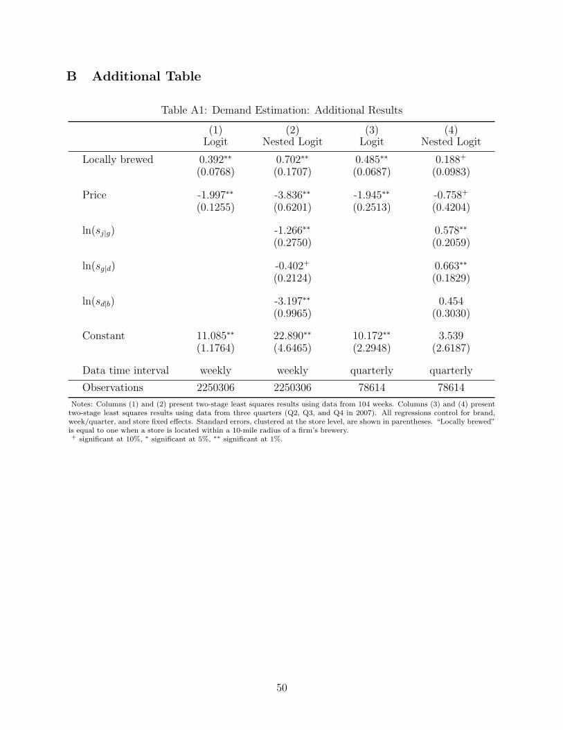
B Additional Table

Table A1: Demand Estimation: Additional Results

(1) (2) (3) (4)Logit Nested Logit Logit Nested Logit

Locally brewed 0.392∗∗ 0.702∗∗ 0.485∗∗ 0.188+

(0.0768) (0.1707) (0.0687) (0.0983)

Price -1.997∗∗ -3.836∗∗ -1.945∗∗ -0.758+

(0.1255) (0.6201) (0.2513) (0.4204)

ln(sj|g) -1.266∗∗ 0.578∗∗

(0.2750) (0.2059)

ln(sg|d) -0.402+ 0.663∗∗

(0.2124) (0.1829)

ln(sd|b) -3.197∗∗ 0.454(0.9965) (0.3030)

Constant 11.085∗∗ 22.890∗∗ 10.172∗∗ 3.539(1.1764) (4.6465) (2.2948) (2.6187)

Data time interval weekly weekly quarterly quarterly

Observations 2250306 2250306 78614 78614

Notes: Columns (1) and (2) present two-stage least squares results using data from 104 weeks. Columns (3) and (4) presenttwo-stage least squares results using data from three quarters (Q2, Q3, and Q4 in 2007). All regressions control for brand,week/quarter, and store fixed effects. Standard errors, clustered at the store level, are shown in parentheses. “Locally brewed”is equal to one when a store is located within a 10-mile radius of a firm’s brewery.+ significant at 10%, ∗ significant at 5%, ∗∗ significant at 1%.

50