estimating the innovator’s dilemma: structural analysis...

Estimating the Innovator’s Dilemma:Structural Analysis of Creative Destruction

Mitsuru Igami∗

May 30, 2013

Abstract

Theories predict cannibalization between existing and new products delays incum-bents’ innovation, whereas preemptive motives accelerate it, and incumbents’ cost(dis)advantage relative to entrants would further reinforce these tendencies. To empir-ically assess these three forces, I develop and estimate a dynamic oligopoly model usinga unique panel dataset of hard disk drive (HDD) manufacturers (1981–98). The resultssuggest that despite strong preemptive motives and a substantial cost advantage overentrants, incumbents are reluctant to innovate because of cannibalization, which canexplain at least 51% of the incumbent-entrant timing gap. I then assess hypotheticalpolicy interventions including broad patents and trade barriers, and find the industry’swelfare trajectory difficult to outperform, as Schumpeter (1942) conjectured.

Keywords: Creative Destruction, Dynamic Oligopoly, Structural Estimation∗Yale Department of Economics. E-mail: [email protected]. I thank my dissertation advisers

at UCLA: Daniel Ackerberg, Hugo Hopenhayn, Edward Leamer, Mariko Sakakibara, Connan Snider, andRaphael Thomadsen. For suggestions, I thank Ron Adner, Lanier Benkard, Steven Berry, Michael Dickstein,Pinelopi Goldberg, Jinyong Hahn, Philip Haile, Phillip Leslie, Rosa Matzkin, Matthew Mitchell, IchiroObara, Ariel Pakes, Marc Rysman, Kosuke Uetake, Yong Hyeon Yang, and Mark Zbaracki, as well asseminar participants at IIOC, TADC, REER, AEA, and various universities. I thank Clayton Christensenfor encouraging a new approach to the innovator’s dilemma, Minha Hwang for sharing engineering expertise,and James Porter, late editor of DISK/TREND Reports, for sharing industry knowledge and the reports.Financial support from the Nozawa Fellowship, the UCLA CIBER, and the Dissertation Year Fellowshipis gratefully acknowledged. An earlier version of the paper received the Best Student Paper Award at the11th Annual REER at Georgia Tech and the Dreze Award for the best paper by a PhD student at UCLAAnderson.

1

1 Introduction

“In the long run we are all dead,”1 and firms and technologies are no exception. Netflix’smovie download service has grown fast, whereas Blockbuster, a once-dominant DVD rentalchain, filed for bankruptcy protection in 2010 after a reluctant pursuit of an online distribu-tion service. Amazon is now selling everything from electronic books to disposable diapers,whereas Borders, America’s number-two book retailer, liquidated its shops in 2011 afterbelated efforts to introduce its own electronic reader. These examples may seem extreme,but even when introducing a new technology is not too difficult, the old winners tend notto adapt well while the new entrants quickly become successful, according to a former CEOof Intel, the world’s biggest chip maker (Grove 1996). Some incumbents never introducea new technology/product despite shrinking demand for their existing products, a puzzlingphenomenon called the innovator’s dilemma (Christensen 1997). The timing of innovation ingeneral and the incumbent-entrant timing gap in particular are important for both businessesand policymakers. Who innovates and survives better (and why) is a central question forindividual firms. Depending on how incumbents’ and entrants’ incentives differ, competitionand innovation policies will have different consequences. Understanding the determinants ofthe timing gap is the first step toward designing a pro-innovation competition policy (Bres-nahan 2003). For these purposes, this paper empirically tests three theoretical determinantsof incumbents’ innovation.2

Why do incumbents delay innovation? Viewed from a microeconomic perspective, thedeterminants of innovation timing include (1) cannibalization, (2) different costs, (3) pre-emption, and (4) institutional environment (Hall 2004, Stoneman and Battisti 2010). First,because of cannibalization, the benefits of introducing a new product are smaller for incum-bents than for entrants, to the extent that the old and new goods substitute for each other.By introducing new goods, incumbents are merely replacing their old source of profits, soArrow (1962) calls this mechanism the “replacement effect.” Second, incumbents may facehigher costs of innovation because of organizational inertia. Economic theory, as well as casestudies, suggest that as firms grow larger and older, their R&D efficiency diminishes (e.g.,Schumpeter 1934);3 although, a priori, hypothesizing that incumbency confers some advan-

1John Maynard Keynes, A Tract on Monetary Reform (1923), Ch. 3.2Following Schumpeter’s (1934) view, this paper uses the words “innovation” and “technology adoption”

interchangeably, and avoids equating innovation with “invention,” which may or may not constitute inno-vation in the economic sense. In the HDD industry, the technological roadmap and the future productstandards (i.e., new concepts) are widely shared, whereas the actual commercialization and product devel-opment are left to individual firms’ efforts. This paper takes the former (i.e., shared conceptualization) asexogenously given, and analyzes the latter (i.e., commercialization) as endogenous decisions.

3The existing literature suggests various reasons for incumbents’ inertia, such as bureaucratization(Schumpeter 1934), hierarchy (Sah and Stiglitz 1986), loss of managerial control (Scherer and Ross 1990),

2

tages due to accumulated R&D capital is equally plausible (e.g., Schumpeter 1942). Hence,whether incumbents have a cost advantage or disadvantage is an open empirical question.Third, market structure dynamics play an important, countervailing role, as theories pre-dict incumbents should innovate more aggressively than entrants to preempt potential rivals(e.g., Gilbert and Newbury 1982) under various oligopolistic settings. Finally, the impactof these three determinants will change under different institutional contexts, such as therules governing patents and international trade. In total, these three competing forces (plusinstitutional contexts) determine innovation timing. Cannibalization delays incumbents’ in-novation, whereas preemptive motives accelerate it, and incumbents’ cost (dis)advantagewould further reinforce these tendencies. Given this tug of war between the three theoret-ical forces, I propose to explicitly incorporate them into a unified model and estimate theempirical importance of each.

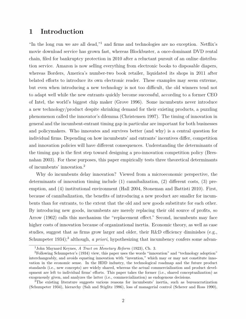
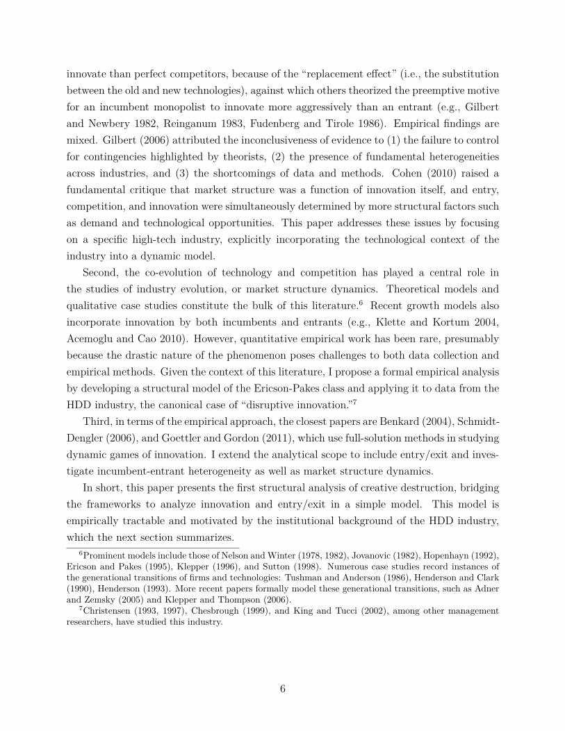
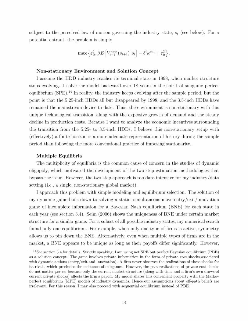
Figure 1: Shifting Generations of Technology

�

�

�

� �

� �

� �

� �

� �

� �

� � � ��

� ��

� ��

� ��

� ��

�� !"�#�� !"�#�� !"�#�� !"�#��

� $ % � & ' $ % � & ' �#( � � $ % � & ' �#( � $ % � & ' �#( � $ % � & '

Note: Shipment-based recognition of firms. Major firms only.

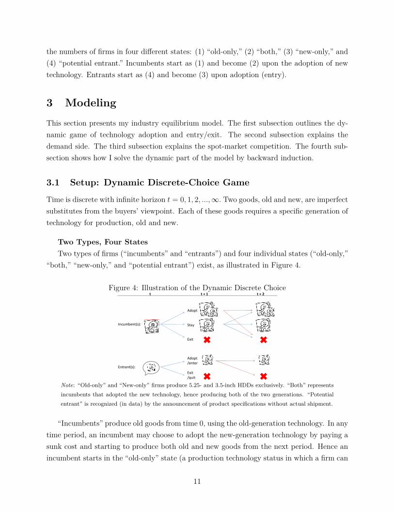
The goal of this paper is to provide the first structural econometric account of creativedestruction (Schumpeter 1942) and empirically quantify these competing forces behind theinnovator’s dilemma in the HDD industry, which is a highly relevant setting. As epitomizedby Christensen (1997), this industry is a canonical case of creative destruction, where cohortsof firms come and go with the generational transitions of technologies (Figure 1). I constructa unique dataset from the industry publications, DISK/TREND Reports (1977–99), whichrecord a comprehensive set of firms (both incumbents and potential entrants) for more thantwo decades. An HDD is a component of a personal computer (PC) that stores information.Desktop PCs used 5.25-inch HDDs during the 1980s, but 3.5-inch HDDs became popular

and informational, cognitive, or relationship reasons (Grove 1996, Christensen 1997).

3

during the 1990s, so those firms that exclusively manufactured 5.25-inch HDDs disappearedby the turn of the century.

The task of quantifying the three forces calls for a structural approach, because incen-tives to innovate are sensitive to an industry’s technological and institutional context. Ibuild and estimate a dynamic oligopoly model that explicitly incorporates cannibalization,heterogeneous innovation costs, and preemptive motives (dynamic strategic interactions),all of which endogenously determine the timing of innovation and the evolution of marketstructure. Then I measure the effects of the three forces by contrasting the outcome of theestimated model with those of three counterfactual simulations in which firms ignore eachof these incentives. Finally, to study broader implications of the phenomenon, I simulateevolutions of the industry under two alternative institutional settings: (1) a broad patentregime and (2) a ban on foreign goods.4

My modeling and estimation approach proceeds in three steps. First, I estimate demandusing a standard discrete choice model for differentiated goods (the old- and new-generationHDDs). That is, I let the data tell the degree of substitution between the old and new goodsand hence of cannibalization. Second, I recover marginal costs of production, implied by thefirst-order conditions of static competition (multi-product Cournot). From these demandand cost estimates, I calculate the static equilibrium profits in every state of the industry,that is, given any number of active firms in the market. These profit estimates embodythe relationship between market structure and profitability and hence give a preliminaryindication of the extent to which preemption motivates firms’ introduction of a new technol-ogy/product. Third, I feed these static (period) profits into a dynamic model to estimate thesunk costs of innovation. The model features two types of firms, incumbents and entrants,so I estimate the sunk costs separately for each type. I explicitly incorporate firms’ dynamicdiscrete choice between entering, exiting, continuing operation with the old product, or in-troducing the new product. I fully incorporate preemptive motives, because firms interactstrategically and are forward-looking with rational expectations over the endogenous evolu-tion of market structure. To reflect the uniqueness of the technological transition in HDDsas well as the computer industry’s ever-changing nature, I make my model non-stationary,allowing demand, costs, and hence value and policy functions to change over time.

Conceptually, this third step is simple. I invoke a revealed preference argument and em-ploy maximum likelihood estimation (MLE), with nested fixed-point (NFXP) algorithm, tofind the sunk cost parameter values that would best rationalize the actual innovation andentry/exit behaviors in the data.5 Practically, however, this procedure poses two technical

4Appendix reports additional simulation results for theoretical benchmarks and two more policy experi-ments concerning competition and innovation (entry deregulation and R&D subsidies for incumbents).

5I have chosen to use NFXP because this paper studies non-stationary industry dynamics in a single, global

4

challenges. One is the possibility of multiple equilibria. I address this issue through parsi-monious modeling (a small state space and choice sets, and period-by-period, state-by-statesolutions) to achieve uniqueness in some industry states, while relying on equilibrium se-lection in other cases (see section 3.1 for details). The other problem is the computationalburden of calculating the equilibrium strategies and values, for each of the several thousandindustry states, in each of the 18 years, for each set of candidate parameter values. I ad-dress this issue by coding the most computationally expensive routines (the calculation ofexpected values) in the C language within the MATLAB platform.

The estimation and simulation results suggest that despite strong preemptive motivesand a substantial cost advantage over entrants, incumbents are reluctant to innovate earlybecause of cannibalization, which can explain at least 51% of the timing gap. Incumbentsmay lag behind entrants, despite their advantage in innovation costs, which suggests a sub-stantial part of what researchers have previously understood as organizational inertia couldpotentially be reinterpreted as an effect of cannibalization. The results from the policysimulations highlight the pro-innovation effect of competition. For example, I find a banon international trade discourages innovation and hurts consumers. However, social welfaresometimes improves under anti-competitive policies, such as broad patents. Ironically, wel-fare improves not through promotion of innovation, but through cost savings from preventing“excess” entry/innovation.

I have organized the rest of the paper as follows. The remainder of this section explainshow this research contributes to the literature on innovation and industry dynamics. Section2 summarizes the technological and institutional background of the HDD industry. Section 3describes the model. Sections 4 and 5 explain the estimation procedure and results. Section6 quantifies the three economic forces behind “the innovator’s dilemma.” Section 7 evaluateswelfare consequences of different policies in innovation and competition. Section 8 concludes.

1.1 Related Literature

This paper uses a structural approach to study the process of creative destruction. As such,it builds on three bodies of literature: innovation, industry dynamics, and the estimation ofdynamic games.

First, many papers have studied the relationship between competition and innovation,with mixed predictions and inconclusive evidence (see Gilbert [2006] and Cohen [2010] fordetailed surveys). Arrow (1962) predicted an incumbent monopolist has less incentive to

market, which makes the use of other approaches difficult, such as two-step estimation and mathematicalprogramming with equilibrium constraints (MPEC).

5

innovate than perfect competitors, because of the “replacement effect” (i.e., the substitutionbetween the old and new technologies), against which others theorized the preemptive motivefor an incumbent monopolist to innovate more aggressively than an entrant (e.g., Gilbertand Newbery 1982, Reinganum 1983, Fudenberg and Tirole 1986). Empirical findings aremixed. Gilbert (2006) attributed the inconclusiveness of evidence to (1) the failure to controlfor contingencies highlighted by theorists, (2) the presence of fundamental heterogeneitiesacross industries, and (3) the shortcomings of data and methods. Cohen (2010) raised afundamental critique that market structure was a function of innovation itself, and entry,competition, and innovation were simultaneously determined by more structural factors suchas demand and technological opportunities. This paper addresses these issues by focusingon a specific high-tech industry, explicitly incorporating the technological context of theindustry into a dynamic model.

Second, the co-evolution of technology and competition has played a central role inthe studies of industry evolution, or market structure dynamics. Theoretical models andqualitative case studies constitute the bulk of this literature.6 Recent growth models alsoincorporate innovation by both incumbents and entrants (e.g., Klette and Kortum 2004,Acemoglu and Cao 2010). However, quantitative empirical work has been rare, presumablybecause the drastic nature of the phenomenon poses challenges to both data collection andempirical methods. Given the context of this literature, I propose a formal empirical analysisby developing a structural model of the Ericson-Pakes class and applying it to data from theHDD industry, the canonical case of “disruptive innovation.”7

Third, in terms of the empirical approach, the closest papers are Benkard (2004), Schmidt-Dengler (2006), and Goettler and Gordon (2011), which use full-solution methods in studyingdynamic games of innovation. I extend the analytical scope to include entry/exit and inves-tigate incumbent-entrant heterogeneity as well as market structure dynamics.

In short, this paper presents the first structural analysis of creative destruction, bridgingthe frameworks to analyze innovation and entry/exit in a simple model. This model isempirically tractable and motivated by the institutional background of the HDD industry,which the next section summarizes.

6Prominent models include those of Nelson and Winter (1978, 1982), Jovanovic (1982), Hopenhayn (1992),Ericson and Pakes (1995), Klepper (1996), and Sutton (1998). Numerous case studies record instances ofthe generational transitions of firms and technologies: Tushman and Anderson (1986), Henderson and Clark(1990), Henderson (1993). More recent papers formally model these generational transitions, such as Adnerand Zemsky (2005) and Klepper and Thompson (2006).

7Christensen (1993, 1997), Chesbrough (1999), and King and Tucci (2002), among other managementresearchers, have studied this industry.

6

2 Industry and Data

This section describes the key features of the HDD industry and explains why it is particularlysuitable for the study of innovation and industry evolution.

2.1 HDD: Canonical Case of Creative Destruction

The HDD industry provides a particularly fruitful example for the study of technologicalchange and industry dynamics.

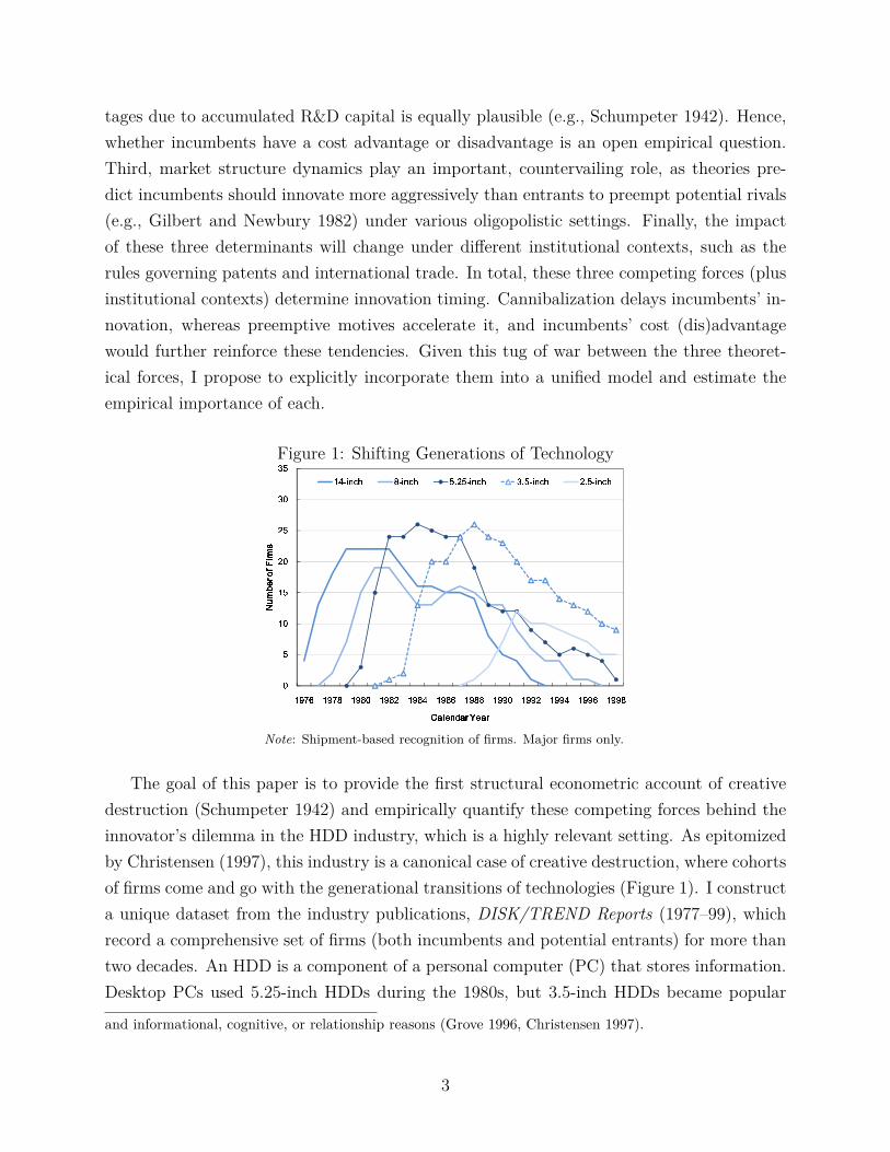
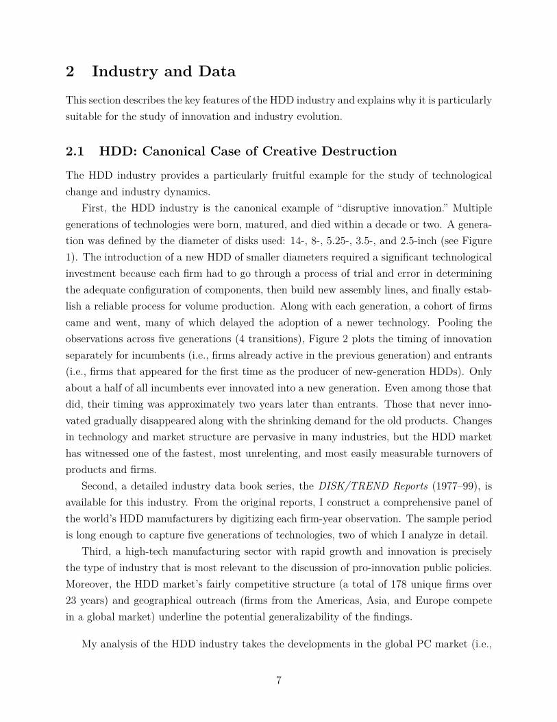
First, the HDD industry is the canonical example of “disruptive innovation.” Multiplegenerations of technologies were born, matured, and died within a decade or two. A genera-tion was defined by the diameter of disks used: 14-, 8-, 5.25-, 3.5-, and 2.5-inch (see Figure1). The introduction of a new HDD of smaller diameters required a significant technologicalinvestment because each firm had to go through a process of trial and error in determiningthe adequate configuration of components, then build new assembly lines, and finally estab-lish a reliable process for volume production. Along with each generation, a cohort of firmscame and went, many of which delayed the adoption of a newer technology. Pooling theobservations across five generations (4 transitions), Figure 2 plots the timing of innovationseparately for incumbents (i.e., firms already active in the previous generation) and entrants(i.e., firms that appeared for the first time as the producer of new-generation HDDs). Onlyabout a half of all incumbents ever innovated into a new generation. Even among those thatdid, their timing was approximately two years later than entrants. Those that never inno-vated gradually disappeared along with the shrinking demand for the old products. Changesin technology and market structure are pervasive in many industries, but the HDD markethas witnessed one of the fastest, most unrelenting, and most easily measurable turnovers ofproducts and firms.

Second, a detailed industry data book series, the DISK/TREND Reports (1977–99), isavailable for this industry. From the original reports, I construct a comprehensive panel ofthe world’s HDD manufacturers by digitizing each firm-year observation. The sample periodis long enough to capture five generations of technologies, two of which I analyze in detail.

Third, a high-tech manufacturing sector with rapid growth and innovation is preciselythe type of industry that is most relevant to the discussion of pro-innovation public policies.Moreover, the HDD market’s fairly competitive structure (a total of 178 unique firms over23 years) and geographical outreach (firms from the Americas, Asia, and Europe competein a global market) underline the potential generalizability of the findings.

My analysis of the HDD industry takes the developments in the global PC market (i.e.,

7

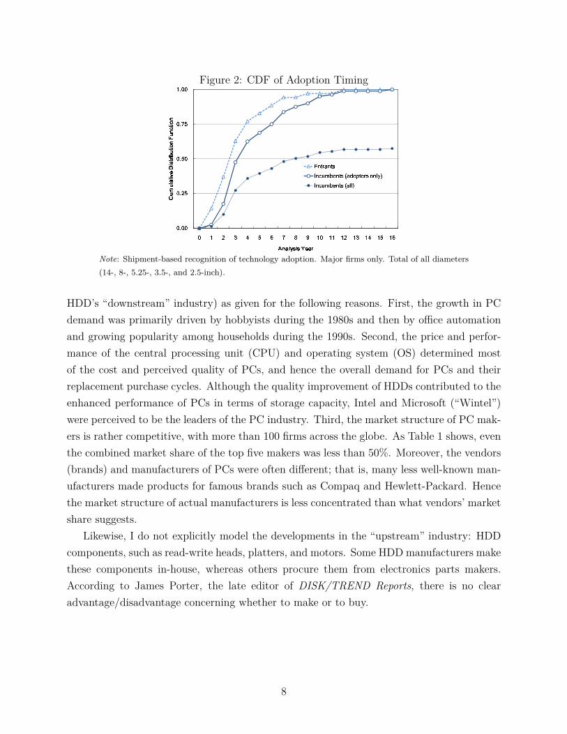
Figure 2: CDF of Adoption Timing

�

��

��

��

��

� � � �

��

� �� !�"�� #$% �$&�� #$

� �� !�"�� #$% �$&�� #$

� �� !�"�� #$% �$&�� #$

� �� !�"�� #$% �$&�� #$

')( *,+ - . / .1032 * 4')( *,+ - . / .1032 * 4')( *,+ - . / .1032 * 4')( *,+ - . / .1032 * 4

5,( 6 4 *7( 6 .8 ( 9 : ;=< 27( 6 .3> * ? @7A 6 274 .1@7( + - B8 ( 9 : ;=< 27( 6 .3> *7+ + B

Note: Shipment-based recognition of technology adoption. Major firms only. Total of all diameters(14-, 8-, 5.25-, 3.5-, and 2.5-inch).

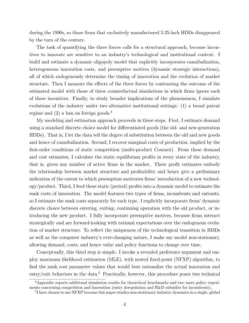
HDD’s “downstream” industry) as given for the following reasons. First, the growth in PCdemand was primarily driven by hobbyists during the 1980s and then by office automationand growing popularity among households during the 1990s. Second, the price and perfor-mance of the central processing unit (CPU) and operating system (OS) determined mostof the cost and perceived quality of PCs, and hence the overall demand for PCs and theirreplacement purchase cycles. Although the quality improvement of HDDs contributed to theenhanced performance of PCs in terms of storage capacity, Intel and Microsoft (“Wintel”)were perceived to be the leaders of the PC industry. Third, the market structure of PC mak-ers is rather competitive, with more than 100 firms across the globe. As Table 1 shows, eventhe combined market share of the top five makers was less than 50%. Moreover, the vendors(brands) and manufacturers of PCs were often different; that is, many less well-known man-ufacturers made products for famous brands such as Compaq and Hewlett-Packard. Hencethe market structure of actual manufacturers is less concentrated than what vendors’ marketshare suggests.

Likewise, I do not explicitly model the developments in the “upstream” industry: HDDcomponents, such as read-write heads, platters, and motors. Some HDD manufacturers makethese components in-house, whereas others procure them from electronics parts makers.According to James Porter, the late editor of DISK/TREND Reports, there is no clearadvantage/disadvantage concerning whether to make or to buy.

8

Table 1: Global PC Market Share by Units (%)

Rank 1981 1986 1991 19961 Sinclair 23.9 IBM 12.3 IBM 11.4 Compaq 10.02 Apple 13.6 Commodore 11.4 Apple 9.1 IBM 8.63 Commodore 13.0 Apple 7.8 Commodore 8.3 Packard-Bell NEC 6.04 Tandy 12.8 Amstrad 5.9 NEC 5.8 Apple 5.95 Atari 4.5 NEC 5.3 Compaq 4.0 HP N/AOthers 32.3 57.2 61.5 69.5

Note: Market share based on worldwide unit shipments.Source: Gartner Dataquest, Wikipedia.

2.2 Data Source

I manually construct the panel data of 1,378 firm-year observations from DISK/TRENDReports (1977–99), an annual publication series edited by the HDD experts in Silicon Valley.I digitize each firm-year observation, which is accompanied by half a page of qualitativedescriptions (on the characteristics of the firm, managers, funding, products, productionlocations, as well as major actions taken in that year, with their reasons) in the originalpublication. Not all information is amenable to quantitative analysis, but some of the firms’characteristics are suitable for regressions. For example, firms’ age and size (in terms ofrevenues and profits, either company-wide or specifically for the HDD business) are readilycodifiable.8 Firms’ organizational forms, regions of origin, and the initial HDD generationsin which they started manufacturing, are also digitized as categorical variables.

An auxiliary dataset, also from DISK/TREND Reports, containing the prices and ship-ment quantities of HDDs, accompanies these panel data of firms. For each year, the reportsrecord the average transaction price and total quantity for each of the generation-qualitycategories (5 generations and 14 quality levels in total).

Researchers in both economics and management repeatedly confirm the accuracy, rele-vance, and comprehensiveness of the record.9

2.3 Focus: Transition from 5.25- to 3.5-inch Generations

I analyze the technological transition from the 5.25- to 3.5-inch generations, which I will callthe “old” and “new” generations henceforth. This subsample of the dataset spans 18 years

8However, age is not necessarily comparable across firms that had roots in different industries (e.g.,manufacturers of card punchers, typewriters, automobile components, or coin laundries). Not all firmsdisclosed division-level revenue/profit information. For these reasons, I omit these variables in the followingregressions.

9Christensen (1993, 1997); Lerner (1997); McKendrick, Donner, and Haggard (2000); and Franco andFilson (2006).

9

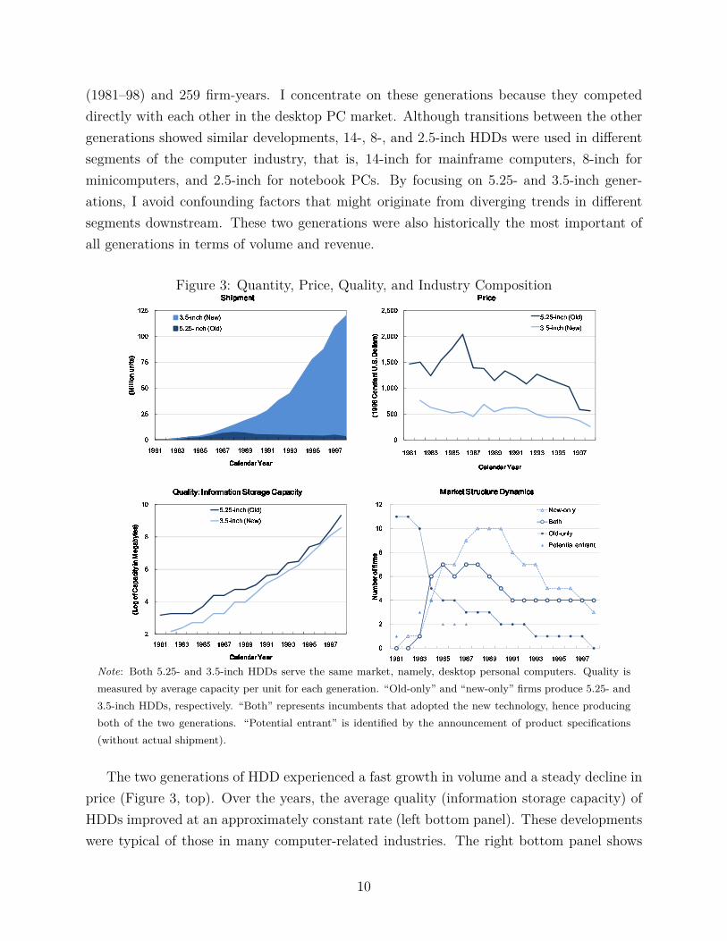
(1981–98) and 259 firm-years. I concentrate on these generations because they competeddirectly with each other in the desktop PC market. Although transitions between the othergenerations showed similar developments, 14-, 8-, and 2.5-inch HDDs were used in differentsegments of the computer industry, that is, 14-inch for mainframe computers, 8-inch forminicomputers, and 2.5-inch for notebook PCs. By focusing on 5.25- and 3.5-inch gener-ations, I avoid confounding factors that might originate from diverging trends in differentsegments downstream. These two generations were also historically the most important ofall generations in terms of volume and revenue.

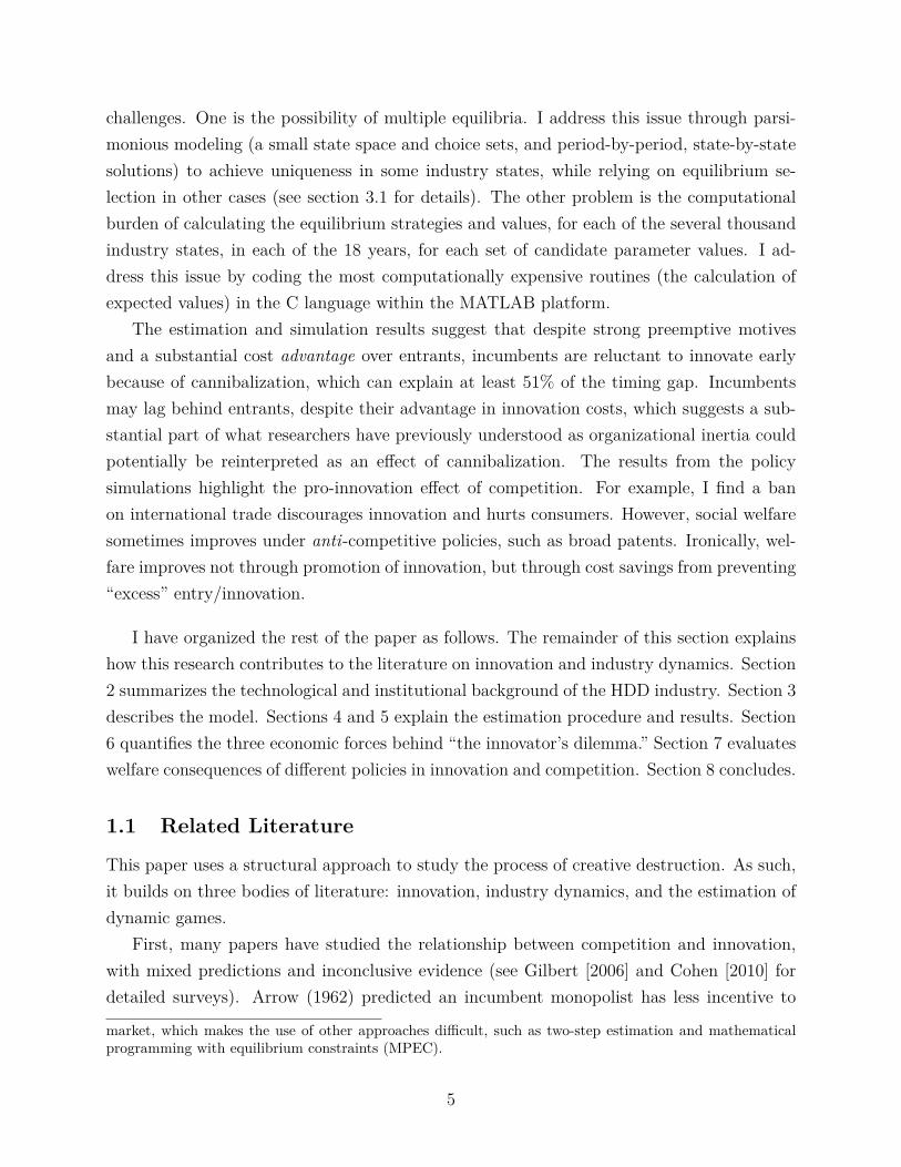
Figure 3: Quantity, Price, Quality, and Industry Composition

�

� �

� �

� �

� � �

� � �

� � � ��

��

��

��

��

� � � � � � � � � � � ��

� � � !#" $ %� � � !#" $ %� � � !#" $ %� � � !#" $ %

� & � ' ( � ) * + , � - .� & � � ' ( � ) * + / � � .

�

� � �

� 0 � � �

� 0 � � �

� 0 � � �

� 0 � � �

� � � �1� � � �1� � � �1� � � �2� � � �1� � � �3� � � �1� � � �2� � � �

�45567 �� 8��9 :; :< �� 8=��

�45567 �� 8��9 :; :< �� 8=��

�45567 �� 8��9 :; :< �� 8=��

�45567 �� 8��9 :; :< �� 8=��

� � � � � � � � � � � ��

> ? � @ "> ? � @ "> ? � @ "> ? � @ "

� & � � ' ( � ) * + / � � .� & � ' ( � ) * + , � - .

�

A

B

�

� �

� � � �1� � � �2� � � �1� � � �2� � � �1� � � �3� � � �1� � � �2� � � �

�C �D�E78F8G � H ��ID8J H�I��

�C �D�E78F8G � H ��ID8J H�I��

�C �D�E78F8G � H ��ID8J H�I��

�C �D�E78F8G � H ��ID8J H�I��

� � � � � � � � � � � ��

KML N O � % P Q R $ S T ? !#N % � T $ � % T ? N U " V N N @ � % PKML N O � % P Q R $ S T ? !#N % � T $ � % T ? N U " V N N @ � % PKML N O � % P Q R $ S T ? !#N % � T $ � % T ? N U " V N N @ � % PKML N O � % P Q R $ S T ? !#N % � T $ � % T ? N U " V N N @ � % P

� & � � ' ( � ) * + / � � .� & � ' ( � ) * + , � - .

W

X

Y

Z

[

\ W

\ X

\ ] [ \\ ] [ ^_\ ] [ `a\ ] [ b_\ ] [ ]a\ ] ] \a\ ] ] ^a\ ] ] `_\ ] ] b

c def ghijjk hel

c def ghijjk hel

c def ghijjk hel

c def ghijjk hel

m#n o p q r s r o t u r t o q v w x n y{z u |m#n o p q r s r o t u r t o q v w x n y{z u |m#n o p q r s r o t u r t o q v w x n y{z u |m#n o p q r s r o t u r t o q v w x n y{z u |

} ~ � � � � � �� ~ � � � � � ~ � � � � � �

Note: Both 5.25- and 3.5-inch HDDs serve the same market, namely, desktop personal computers. Quality ismeasured by average capacity per unit for each generation. “Old-only” and “new-only” firms produce 5.25- and3.5-inch HDDs, respectively. “Both” represents incumbents that adopted the new technology, hence producingboth of the two generations. “Potential entrant” is identified by the announcement of product specifications(without actual shipment).

The two generations of HDD experienced a fast growth in volume and a steady decline inprice (Figure 3, top). Over the years, the average quality (information storage capacity) ofHDDs improved at an approximately constant rate (left bottom panel). These developmentswere typical of those in many computer-related industries. The right bottom panel shows

10

the numbers of firms in four different states: (1) “old-only,” (2) “both,” (3) “new-only,” and(4) “potential entrant.” Incumbents start as (1) and become (2) upon the adoption of newtechnology. Entrants start as (4) and become (3) upon adoption (entry).

3 Modeling

This section presents my industry equilibrium model. The first subsection outlines the dy-namic game of technology adoption and entry/exit. The second subsection explains thedemand side. The third subsection explains the spot-market competition. The fourth sub-section shows how I solve the dynamic part of the model by backward induction.

3.1 Setup: Dynamic Discrete-Choice Game

Time is discrete with infinite horizon t = 0, 1, 2, ..., ∞. Two goods, old and new, are imperfectsubstitutes from the buyers’ viewpoint. Each of these goods requires a specific generation oftechnology for production, old and new.

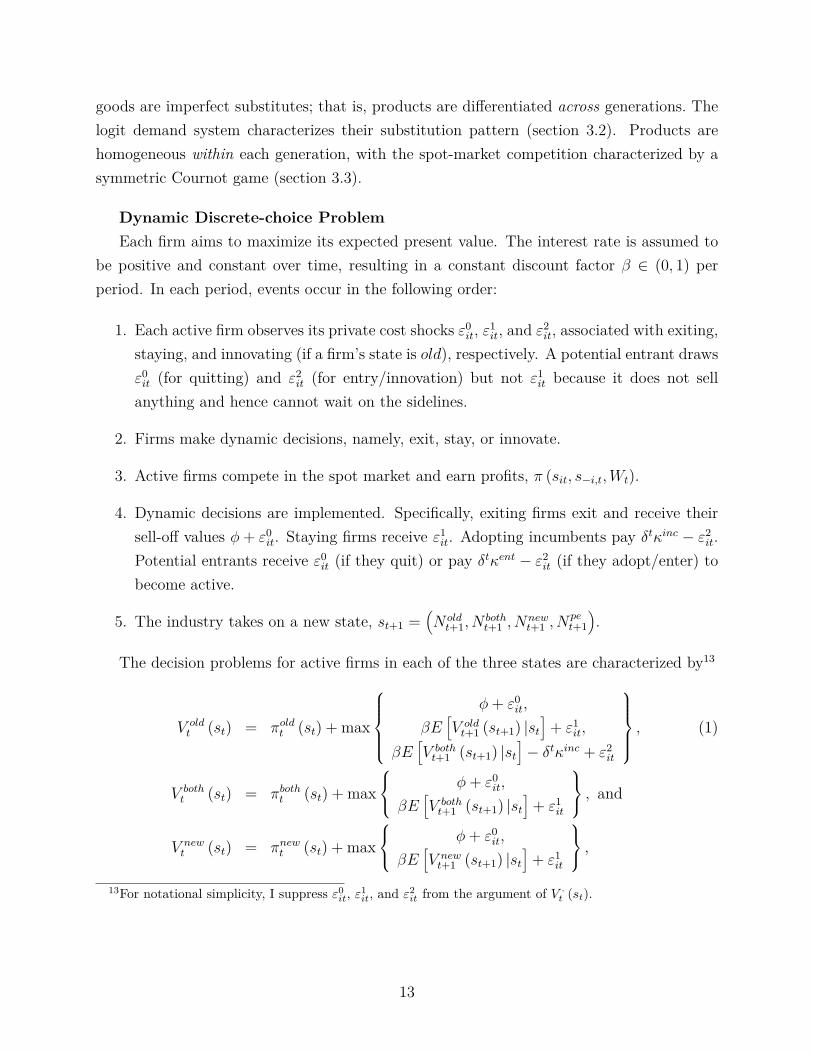
Two Types, Four StatesTwo types of firms (“incumbents” and “entrants”) and four individual states (“old-only,”

“both,” “new-only,” and “potential entrant”) exist, as illustrated in Figure 4.

Figure 4: Illustration of the Dynamic Discrete Choice

��

��

��

��

� � ��

��

��

��

��

��

Note: “Old-only” and “New-only” firms produce 5.25- and 3.5-inch HDDs exclusively. “Both” representsincumbents that adopted the new technology, hence producing both of the two generations. “Potentialentrant” is recognized (in data) by the announcement of product specifications without actual shipment.

“Incumbents” produce old goods from time 0, using the old-generation technology. In anytime period, an incumbent may choose to adopt the new-generation technology by paying asunk cost and starting to produce both old and new goods from the next period. Hence anincumbent starts in the “old-only” state (a production technology status in which a firm can

11

produce only old goods) and may elect to transition to the “both” state (a status in whicha firm can produce both old and new goods).

“Entrants” are the other type of firms. They are not active in the market at time 0. Eachof them appears in a predetermined year (observed in data),10 at which moment they maychoose to adopt new technology and enter the market, or quit the prospect of entry.11 Thatis, by paying a sunk cost, a potential entrant becomes an actual entrant in the subsequentperiod in the “new-only” state, a production technology status in which a firm can produceonly new goods.12

Hence a firm belongs to any one of the four states, sit ∈ {old, both, new, pe}. The industrystate summarizes all firms’ states, st =

(N old

t , N botht , Nnew

t , Npet

), as the numbers of firms in

each of four states. Let s−i,t denote the numbers of competitors for firm i, which is simplyst minus 1 in firm i’s own category.

Period ProfitFirm i’s single-period profit, π (sit, s−i,t, Wt), depends on its own state sit, its competitors’

state s−i,t, and the characteristics of demand and cost Wt. sit and s−i,t change endogenouslyas a result of each firm’s dynamic decision, whereas Wt evolves exogenously. Old and new

10I have also attempted the following alternative modeling approaches: (1) assuming a fixed number ofpotential entrants for all years, (2) assuming the difference between the peak number of active firms acrossall years (in data) and the current number of active firms as the number of potential entrants in that year,(3) assuming infinitely many potential entrants and their sequential free entry, and (4) a combination of(3) and my approach in the paper. Although these modeling approaches have their merits, I have chosento model potential entrants in a more data-driven manner, for the following reasons. Conceptually, theprimary purpose of this research is to empirically analyze incumbents’ decision-making in the presence ofcredible threats of entry, rather than developing some generic model of entry. In this context, the estimationof incumbents’ and entrants’ innovation costs is most meaningful when we compare incumbents and themost serious contenders that are known to exist by the industry participants (and hence recorded in theindustry publications), rather than numerous potential entrants that might be theoretically possible butpractically invisible. Quantitatively my modeling choice will translate into estimating a lower bound ofentrants’ innovation/entry cost. The more potential entrants we assume, the higher the estimated cost ofentry has to be in order to rationalize the number of actual entrants in the data.

11An alternative modeling approach is to allow potential entrants to wait multiple years before actualentry, but I have chosen to characterize them as ephemeral creatures, for three reasons. First, potentialentrants in the data do not wait. They either enter in the following year or disappear from record. Second,no venture capitalist in Silicon Valley appears sufficiently patient to let entrepreneurs wait and burn cashfor multiple years, especially in a fast-changing industry. Third, an empirical model of dynamic oligopolyneeds to define the state space parsimoniously. Given my other modeling choices, potential entrants withlonger life would increase the size of the state space exponentially and make its computation infeasible. Iconjecture that, quantitatively, this modeling choice will affect my estimates in the following manner. Onthe one hand, assuming potential entrants with longer life might lower the entry cost estimate because wewould not need as high an entry cost to rationalize their no entry, although how this logic might interactwith the observational fact that no potential entrant waited multiple years is less obvious. On the otherhand, incumbents might have stronger preemptive motives if potential entrants can wait and are hence lessdesperate to enter, which might alter the equilibrium strategy profile.

12I do not consider entrants’ adoption of the old technology because it rarely happens in the data oncethe new technology becomes available.

12

goods are imperfect substitutes; that is, products are differentiated across generations. Thelogit demand system characterizes their substitution pattern (section 3.2). Products arehomogeneous within each generation, with the spot-market competition characterized by asymmetric Cournot game (section 3.3).

Dynamic Discrete-choice ProblemEach firm aims to maximize its expected present value. The interest rate is assumed to

be positive and constant over time, resulting in a constant discount factor β ∈ (0, 1) perperiod. In each period, events occur in the following order:

1. Each active firm observes its private cost shocks ε0it, ε1

it, and ε2it, associated with exiting,

staying, and innovating (if a firm’s state is old), respectively. A potential entrant drawsε0

it (for quitting) and ε2it (for entry/innovation) but not ε1

it because it does not sellanything and hence cannot wait on the sidelines.

2. Firms make dynamic decisions, namely, exit, stay, or innovate.

3. Active firms compete in the spot market and earn profits, π (sit, s−i,t, Wt).

4. Dynamic decisions are implemented. Specifically, exiting firms exit and receive theirsell-off values φ + ε0

it. Staying firms receive ε1it. Adopting incumbents pay δtκinc − ε2

it.Potential entrants receive ε0

it (if they quit) or pay δtκent − ε2it (if they adopt/enter) to

become active.

5. The industry takes on a new state, st+1 =(N old

t+1, N botht+1 , Nnew

t+1 , Npet+1

).

The decision problems for active firms in each of the three states are characterized by13

V oldt (st) = πold

t (st) + max

φ + ε0

it,

βE[V old

t+1 (st+1) |st

]+ ε1

it,

βE[V both

t+1 (st+1) |st

]− δtκinc + ε2

it

, (1)

V botht (st) = πboth

t (st) + max

φ + ε0it,

βE[V both

t+1 (st+1) |st

]+ ε1

it

, and

V newt (st) = πnew

t (st) + max

φ + ε0it,

βE[V new

t+1 (st+1) |st

]+ ε1

it

,

13For notational simplicity, I suppress ε0it, ε1

it, and ε2it from the argument of V ·

t (st).

13

subject to the perceived law of motion governing the industry state, st (see below). For apotential entrant, the problem is simply

max{ε0

it, βE[V new

t+1 (st+1) |st

]− δtκent + ε2

it

}.

Non-stationary Environment and Solution ConceptI assume the HDD industry reaches its terminal state in 1998, when market structure

stops evolving. I solve the model backward over 18 years in the spirit of subgame perfectequilibrium (SPE).14 In reality, the industry keeps evolving after the sample period, but thepoint is that the 5.25-inch HDDs all but disappeared by 1998, and the 3.5-inch HDDs haveremained the mainstream device to date. Thus, the environment is non-stationary with thisunique technological transition, along with the explosive growth of demand and the steadydecline in production costs. Because I want to analyze the economic incentives surroundingthe transition from the 5.25- to 3.5-inch HDDs, I believe this non-stationary setup with(effectively) a finite horizon is a more adequate representation of history during the sampleperiod than following the more conventional practice of imposing stationarity.

Multiple EquilibriaThe multiplicity of equilibria is the common cause of concern in the studies of dynamic

oligopoly, which motivated the development of the two-step estimation methodologies thatbypass the issue. However, the two-step approach is too data intensive for my industry/datasetting (i.e., a single, non-stationary global market).

I approach this problem with simple modeling and equilibrium selection. The solution ofmy dynamic game boils down to solving a static, simultaneous-move entry/exit/innovationgame of incomplete information for a Bayesian Nash equilibrium (BNE) for each state ineach year (see section 3.4). Seim (2006) shows the uniqueness of BNE under certain marketstructure for a similar game. For a subset of all possible industry states, my numerical searchfound only one equilibrium. For example, when only one type of firms is active, symmetryallows us to pin down the BNE. Alternatively, even when multiple types of firms are in themarket, a BNE appears to be unique as long as their payoffs differ significantly. However,

14See section 3.4 for details. Strictly speaking, I am using not SPE but perfect Bayesian equilibrium (PBE)as a solution concept. The game involves private information in the form of private cost shocks associatedwith dynamic actions (entry/exit and innovation). A firm never observes the realizations of these shocks forits rivals, which precludes the existence of subgames. However, the past realizations of private cost shocksdo not matter per se, because only the current market structure (along with time and a firm’s own draws ofcurrent private shocks) affects the firm’s payoff. My model shares this convenient property with the Markovperfect equilibrium (MPE) models of industry dynamics. Hence our assumptions about off-path beliefs areirrelevant. For this reason, I may also proceed with sequential equilibrium instead of PBE.

14

for the other subset of industry states, I do encounter multiple BNE. In such cases, I selectthe first BNE that is reached in best-response iterations that start from the same symmetricstrategy profile.15

I also investigated the effectiveness of an alternative “selection” approach by imposingsequential moves within each state-year, instead of simultaneous moves, which would elimi-nate multiplicity in the current context. However, after several months of trial and error, Ifound this approach infeasible and not particularly appealing for two reasons. First, compu-tation became prohibitively expensive, because one has to find late movers’ best responsesto all possible actions of early movers. Computation time increased by the order of 1000,even with a relatively coarse grid for discretizing the action space. Second, this formulationembeds early-mover advantages to those classes of firms that I specify as early movers, inevery state-year, which is not a desirable specification when the research question is aboutthe incumbent-entrant heterogeneity.

Beliefs (Perceived Law of Motion)For rules governing firms’ beliefs about rivals’ moves, s−i,t+1, I assume rational expecta-

tions. That is, a firm correctly perceives how its rivals make dynamic decisions up to privatecost shocks, (ε0

it, ε1it, ε2

it) iid extreme value. This setup allows for dynamic strategic interac-tions, which are a prerequisite for incorporating cannibalization and preemptive motives intothe model.16

With respect to the evolution of demand and production costs, I assume firms’ perfectforesight. This choice reflects my analytical focus on strategic interactions and innovationcosts rather than informational factors related to demand uncertainty. In my view, thisassumption is simplistic but not distortionary, because firms’ beliefs are homogeneous re-gardless of their types or individual state in any given period. Hence it is unlikely to affectthe incumbent-entrant asymmetry this paper tries to explain.17

Model PrimitivesThere are dynamic and static components of model primitives. Dynamic primitives are

the discount factor β, the mean sell-off value φ, the base sunk costs of innovation κinc and κent,15I use this criterion out of practical necessity. As Pesendorfer (2010) notes, “Lyapunov stability of the

best response mapping is not a convincing equilibrium selection rule in private information games.” Su (2012)demonstrates the existence of other (unstable) equilibria for a similar game.

16I “shut down” this feature in one of the counterfactuals (no-preemption case, in section 6.4), wherefirms instead perceive the industry state as evolving exogenously, in the spirit of non-stationary ObliviousEquilibrium (Weintraub, Benkard, Jeziorski, and Van Roy 2008).

17Although learning is beyond the scope of this paper due to data limitations, adaptive expectations andinformation-related topics can be important, including (1) beliefs about new HDDs’ profitability that arepotentially heterogeneous across firms, and (2) the updating of these beliefs through own experimentationand learning from rivals.

15

the annual rate of sunk cost change δ, a dynamic equilibrium concept, and the informationalassumptions made on firms’ perceived law of motion for the industry state.

Static primitives determine the period profit function: demand parameters, cost parame-ters, and a static equilibrium concept. The next two subsections explain the details of thesestatic model components.

3.2 Demand

I capture the substitution pattern across generations of HDDs using the logit model ofdifferentiated products. The dynamic discrete-choice model (section 3.1) captures HDDs’differentiation across generations and assumes homogeneity within each generation. A buyerk purchasing an HDD of generation g enjoys utility,18

ukg = α0 + α1pg + α2I (g = new) + α3xg + ξg + εkg, (2)

where pg is the price, I (g = new) is the indicator of new generation, ξg is the unobservedcharacteristics (most importantly, “design popularity” among buyers, as well as other unob-served attributes such as “reliability”), and εkg is the idiosyncratic taste shock over gener-ations. The outside goods offer the normalized utility uk0 ≡ 0, which represent removableHDDs (as opposed to fixed HDDs) and other storage devices.19

Let ug ≡ α0 + α1pg + α2I (g = new) + α3xg + ξg represent the mean utility from ageneration-g HDD whose market share is msg = exp (ug) /

∑l exp (ul) . The shipment quan-

tity of generation-g HDDs is Qg = msgM , where M is the size of the HDD market includingthe outside goods (removable HDDs and other storage devices). Practically, M reflects alldesktop PCs to be manufactured globally in a given year. Berry’s (1994) inversion providesthe linear relationship,

ln(

msg

ms0

)= α1pg + α2I (g = new) + α3xg + ξg, (3)

where sg represents the market share of HDDs of generation g, and ms0 is the market shareof outside goods (removable HDDs and other devices). The inverse demand is

pg = 1−α1

[− ln

(msg

ms0

)+ α2I (g = new) + α3xg + ξg

]. (4)

18I suppress the time subscript t for the simplicity of notation. The demand side is static in the sensethat buyers make new purchasing decisions every year. This assumption is not restrictive because multi-yearcontracting is not common and hundreds of buyers (computer makers) are present during the sample period.

19Tape recorders, optical disk drives, and flash memory.

16

3.3 Period Competition

The spot-market competition is characterized by multi-product (i.e., old and new goods)Cournot competition.20 Marginal costs of producing old and new goods, mcold and mcnew,are assumed to be common across firms and constant with respect to quantity. Firm i

maximizes profitsπi =

∑g∈Ai

πig =∑

g∈Ai

(pg − mcg) qig (5)

with respect to shipping quantity qig ∀g ∈ Ai, where πig is the profit of firm i in generationg, and Ai is the set of generations produced by firm i. Firm i’s first-order condition withrespect to its output qig is

pg + ∂pg

∂Qg

qig + ∂ph

∂Qg

qih = mcg, (6)

with g, h ∈ {old, new} , g 6= h, if firm i produces both old and new HDDs. The third termon the left-hand side is dropped if a firm makes only one generation.

3.4 Solution of Dynamic Game by Backward Induction

I assume the state stops evolving after year T . Hence the terminal values associated with afirm’s states, siT ∈ {old, both, new}, are

(V old

T , V bothT , V new

T

)=( ∞∑

τ=T

βτ πoldT (sT ) ,

∞∑τ=T

βτ πbothT (sT ) ,

∞∑τ=T

βτ πnewT (sT )

).21 (7)

In year T − 1, an old-only firm’s problem (aside from maximizing its period profit) is

max{φ + ε0

i,T −1, βE[V old

T (sT ) |sT −1]

+ ε1i,T −1, βE

[V both

T (sT ) |sT −1]

− δT −1κinc + ε2i,T −1

}.

I follow Rust (1987) to exploit the property of the logit errors, εit = (ε0it, ε1

it, ε2it), and their

(conditional) independence over time, to obtain a closed-form expression for the expected20Three considerations led to the Cournot assumption. First, unlike automobiles or ready-to-eat cereals,

HDD is a high-tech “commodity.” Buyers chiefly consider its price and category (i.e., form factor and storagecapacity), within which the room for further differentiation is limited. Second, changes in production capacitytake time, and hence the spot market is characterized by price competition given installed capacities. Third,accounting records indicate that despite fierce competition with undifferentiated goods, the HDD makersseemed to enjoy non-zero (albeit razor-thin) profit margins on average.

21Alternatively, I may anchor the terminal values to some auxiliary data (if available) that would coverthe periods after 1998, the final year of my data set. The market capitalization of the surviving firms asof 1998 would be a natural candidate, which, combined with net debt, would represent their enterprisevalues. However, I stopped pursuing this approach because of (1) the survivorship bias, (2) the presence ofconglomerates, and (3) the omission of private firms.

17

value before observing εit,

Eεi,T −1

[V old

T −1 (sT −1, εi,T −1) |sT −1]

= πoldT −1 (sT −1) + γ

+ ln[exp (φ) + exp

(βE

[V old

T (sT ) |sT −1])

+ exp(βE

[V both

T (sT ) |sT −1]

− δT −1κinc)]

,

where γ is the Euler constant. Similar expressions hold for the other two types:

Eεi,T −1

[V both

T −1 (sT −1, εi,T −1) |sT −1]

= πbothT −1 (sT −1) + γ

+ ln[exp (φ) + exp

(βE

[V both

T (sT ) |sT −1])]

,

and

Eεi,T −1

[V new

T −1 (sT −1, εi,T −1) |sT −1]

= πnewT −1 (sT −1) + γ

+ ln [exp (φ) + exp (βE [V newT (sT ) |sT −1])] .

In this manner, I can write the expected value functions from year T all the way back to year0. The associated choice probabilities (policy functions) will provide a basis for the MLE (insection 4.3).

4 Estimation

My empirical approach takes three steps. First, I estimate the system of demand for dif-ferentiated products. Second, I recover the marginal costs of production implied by thedemand estimates and the first-order conditions of the firms’ period-profit maximization.These (static) demand and cost estimates for each year permit the calculation of periodprofit for each class of firms, in each year, under any market structure (industry state).Third, I embed these period-profit estimates into the dynamic discrete game of innovationand entry/exit, which I solve to estimate the sunk costs of innovation and entry/exit.

4.1 Estimation: Demand

Although the dynamic analysis will focus on the generational transition from 5.25 to 3.5-inchHDDs, the empirical demand analysis incorporates more details. In the data, the unit ofobservation is the combination of generation, quality, buyer category, geographical regions,and year t. For notational simplicity, I denote the generation-quality pair by “productcategory” j and suppress subscripts for the latter three dimensions. A buyer k purchasing

18

an HDD of product category j, that is, a combination of generation g (diameter) and qualityx (storage capacity in megabytes), enjoys utility

ukj = α0 + α1pj + α2I (gj = new) + α3xj + ξj + εkj, (8)

where pj is the price, ξj is the unobserved characteristics, and εkj is the idiosyncratic tasteshock that is assumed iid extreme value (over buyers and generation-quality bins); that is,its cumulative distribution function is F (εkj) = exp (− exp (−εkj)). Berry’s (1994) inversionallows the econometrician to run a linear regression,

ln(

msj

ms0

)= α1pj + α2I (gj = new) + α3xj + ξj, (9)

where msj represents the market share of HDDs of category j, and ms0 is the market shareof outside goods (removable HDDs). The coefficients, α0 through α3 and σ, are the tasteparameters, which I estimate using OLS and instrumental variables (IVs).

Sources of IdentificationThe demand parameters are identified by the time-series and cross-sectional variations

in the data (subscripts omitted for notational simplicity) as well as the logit functionalform. Three dimensions of cross-sectional variation exist. First, an HDD’s product category(denoted by j) is a pair of generation and quality. Two generations and 14 discrete qualitylevels exist, according to the industry convention. Second, data are recorded by buyercategory, PC makers and distributors/end-users. Third, data are recorded by geographicalcategory, U.S., and non-U.S.

The OLS estimation relies on the assumption that E [ξj|pj, gj, xj] = 0; that is, the price ofa category-j HDD is uncorrelated with that particular category’s unobserved attractivenessto the buyers. However, one might suspect a positive correlation between them because anattractive product category would command both higher willingness to pay and higher costof production.

In the IV estimation, I use the following variables as instruments for pj: (1) the prices inthe other region and user category, (2) the number of product “models” (not firms), (3) thenumber of years since first appearance, and (4) the time-series “innovations” in ξjt, νjt. Thefirst IV is used by Hausman (1996) and then by Nevo (2001). The identifying assumptionis that production cost shocks are correlated across markets, whereas taste shocks are not.This assumption reflects the industry context in which HDD makers from across the globecompete in both the United States and elsewhere, whereas end users of HDDs (and hence ofPCs) are more isolated geographically.

19

The second IV was used by Bresnahan (1981) and Berry et al. (1995) and exploits theproximity of rival products (in product space), that is, the negative correlation betweenthe number of “models,” markup, and price in oligopolies. The identifying assumption isthat taste shocks in any given period are not correlated with the number of “models” in aparticular product category j, which are outside my model.22

The third IV relies on steady declines in the marginal costs of production over years.In the HDD industry, costs dropped because of design improvements, reduced costs of keycomponents, and offshore production in Singapore, Malaysia, Thailand, and the Philippines.This overall tendency holds at the product category level as well. The identifying assumptionis that taste shocks are not correlated with such time patterns on the cost side, which I assumeis exogenously determined by advances in engineering.

These three IVs have been used with cross-sectional data and static competition in theliterature, but their usefulness is unknown in the context of global industry dynamics. Forthis reason, I also investigated the results based on an alternative, time-series IV strategy inthe style of Sweeting (2012), and obtained the price coefficient estimates of approximately−3.20, a range statistically indistinguishable at the 5% level from my preferred estimateof −3.28 based on the other three IVs (see section 5.1, column 4 of Table 2). This fourthIV employs an additional identifying assumption that the unobserved quality, ξjt, evolvesaccording to an AR(1) process,

ξjt = ρξjt−1 + νjt,

where ρ is the autoregressive parameter,23 and νjt is the “innovation” (in the time-seriessense) that is assumed iid across product categories and over time. We can form exclusionrestrictions for νjt by assuming firms at t do not know the unpredictable parts νjt+1 whenthey make dynamic decisions.24

22The following observation motivates this IV. Firms need to make “model”-introduction decisions inprior years, without observing taste shocks in particular regions/user types in the following years. Moreimportantly, such dynamic decisions are driven by the sum of discounted present values of future profits,which is affected only negligibly by taste shocks in any particular period, regions, or user types. Hence thisidentifying assumption would be plausible as long as particular regions’/user types’ taste shocks are notextremely serially correlated.

23The estimate for ρ is .41.24I intend this additional IV result as a robustness check and do not use it for the subsequent analysis of

dynamics, because the AR(1) assumption on the demand side may potentially introduce some conceptualinconsistency with my other assumptions on the supply-side dynamics, in which I let firms form perfectforesight about the evolution of demand (for the purpose of alleviating the computational costs). In anycase, even if we use −3.20 instead of −3.28, the subsequent results do not change materially.

20

4.2 Estimation: Marginal Costs

For each year, we can infer the marginal costs of production, mcold and mcnew, from equation(6), namely, the first-order conditions for the firms’ static profit maximization problems.Because the unit observation in the HDD sales data is product category level–and not firmor brand level–I maintain, as identifying assumptions, symmetry across firms (up to privatecost shocks) and constant marginal cost with respect to quantity.

4.3 Estimation: Sunk Costs of Innovation

I do not intend to estimate the discount factor, β, because its identification is known to beimpractical in most cases (c.f., Rust 1987). Likewise, the rate of drop in sunk costs, δ, isdifficult to estimate directly from the following procedure, so instead I will assume δ equalsthe average rate of decline in mcnew over time.25

The contribution of an old firm i in year t to the likelihood is

f old(dit|st; φ, κinc, δ

)= prold (dit = exit)I(dit=exit) prold (dit = stay)I(dit=stay)

prold (dit = adopt)I(dit=adopt) ,

where prold (·) is the probability that an old-only firm takes a particular action dit:

prold (dit = exit) = exp (φ) /A,

prold (dit = stay) = exp(EεV

oldt+1 (st+1)

)/A, and

prold (dit = adopt) = exp(EεV

botht+1 (st+1) − δtκinc

)/A,

where A ≡ exp (φ) + exp(EεV

oldt+1 (st+1)

)+ exp

(EεV

botht+1 (st+1) − δtκinc

). The contributions

of the other three types of firms take similar forms (see Appendix).Year t has Nt ≡

(N old

t , N botht , Nnew

t , Npet

)active firms in each state, of which Xt ≡(

Xoldt , Xboth

t , Xnewt

)exit and Et ≡

(Eold

t , Epet

)innovate. Denote the joint likelihood for

year t of observing data (Nt, Xt, Et) by P (Xt, Et, Nt). Then the overall joint likelihood fort = 0, 1, 2, ..., T − 1 is P (X, E, N) = ∏T −1

t=0 P (Xt, Et, Nt) . Thus the ML estimators for themean sell-off value φ and the base sunk costs of technology adoption κinc and κent are

arg maxφ,κinc,κent

ln [P (X, E, N)] .

25See section 5.2 for details and alternative assumptions.

21

Sources of IdentificationIntuitively, I rely on a revealed-preference argument to identify the sell-off value and

the sunk costs. Algorithmically, this estimation approach searches for the parameter valuesof (φ, κinc, κent) that best rationalize the observed choice probabilities of innovation andentry/exit in data. Thus the key source of identification is variations in entry/exit/innovationdecisions over time and across the four firm classes. For example, φ will depend on thefraction of active firms that exited (in the data), conditional on year and market structure(which determine the payoffs based on the period-profit estimates and the dynamic gamemodel). Likewise, κinc and κent will mostly depend on the observed fractions of innovatingincumbents and potential entrants, respectively.

5 Results

This section reports the estimation results.

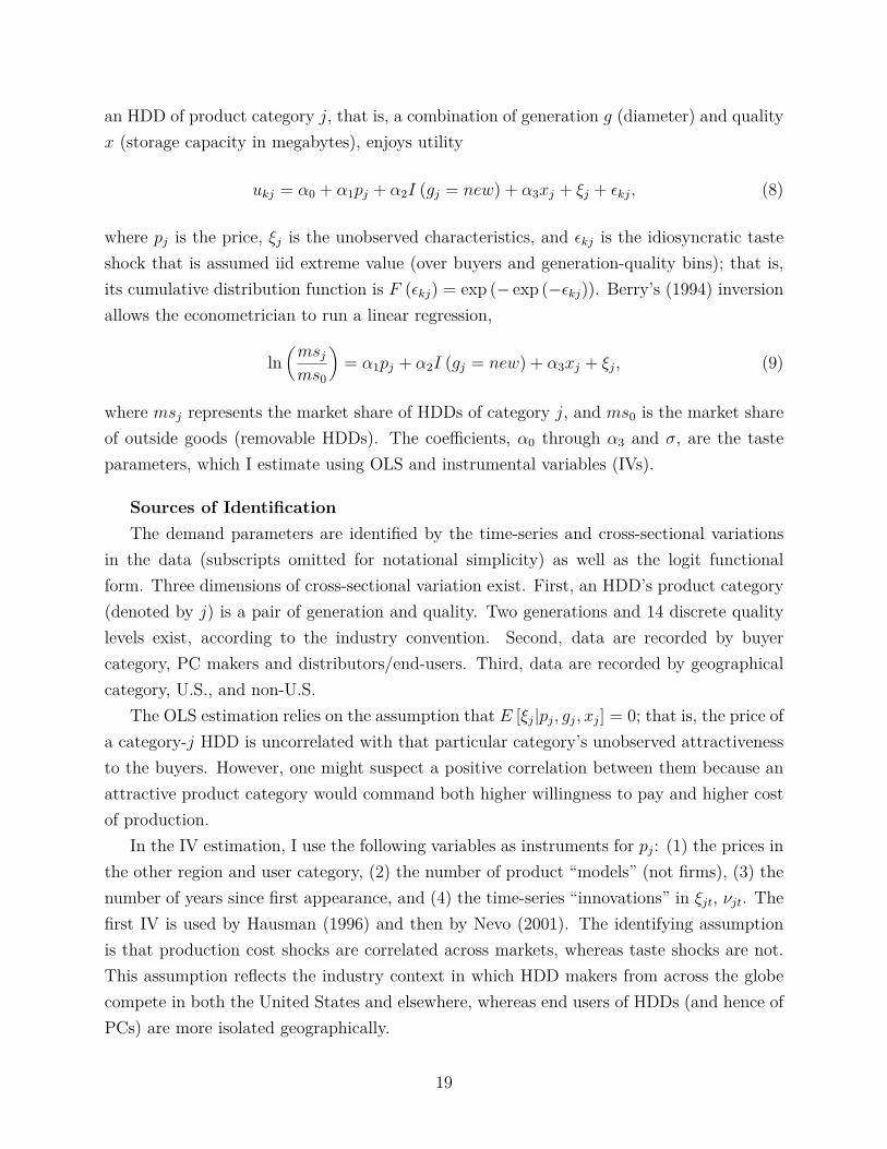
5.1 Results: Demand

Table 2 displays demand estimates. I employ two market definitions, broad (1 and 2) and nar-row (3 and 4). The former definition aggregates observations across both regions (U.S. andnon-U.S.) and user types (computer makers and distributors/end users), in a manner con-sistent with the industry’s context of a single, global market. However, the dataset containsricher variations across regions and user types, which we can exploit for improved precisionof estimates. Moreover, the Hausman-Nevo IVs become available under the narrower marketdefinition (i.e., by region/user type).

The IV estimates in columns (2) and (4) are generally more intuitive and highly sta-tistically significant than the OLS estimates in columns (1) and (3). The price coefficientis negative (α1 < 0), whereas both smaller size (3.5-inch diameter = new generation) andquality (the log of storage capacity) confer higher benefits (α2 > 0, α3 > 0) to the buyers.

I use column (4), the logit IV estimates under the narrow market definition, as mybaseline result for the subsequent analyses. I avoid using the results based on the broadermarket definition. Specifically, result (2) is similar to (4) and highly intuitive, but I amconcerned about the limited availability of IVs and the reduced variation in data.

All four estimates incorporate year dummies and also allow for the time-varying un-observed product quality by diameter (ξjt in equations [8] and [9]; note I suppress time-subscripts in these formulae for notational simplicity). I use equation (9) to recover ξjt asresiduals. Figure 5 (left panel) shows the evolution of ξjt for both old and new HDDs, which

22

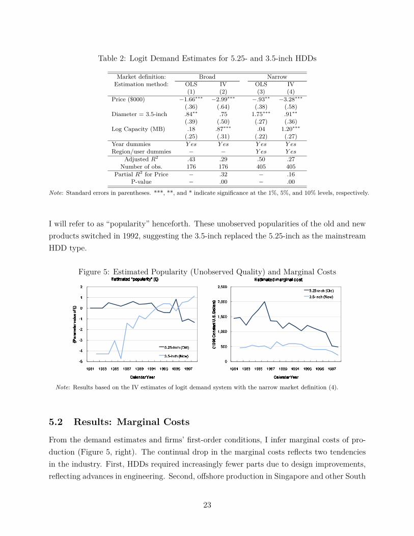
Table 2: Logit Demand Estimates for 5.25- and 3.5-inch HDDs

Market definition: Broad NarrowEstimation method: OLS IV OLS IV

(1) (2) (3) (4)Price ($000) −1.66∗∗∗ −2.99∗∗∗ −.93∗∗ −3.28∗∗∗

(.36) (.64) (.38) (.58)Diameter = 3.5-inch .84∗∗ .75 1.75∗∗∗ .91∗∗

(.39) (.50) (.27) (.36)Log Capacity (MB) .18 .87∗∗∗ .04 1.20∗∗∗

(.25) (.31) (.22) (.27)Year dummies Y es Y es Y es Y esRegion/user dummies − − Y es Y es

Adjusted R2 .43 .29 .50 .27Number of obs. 176 176 405 405

Partial R2 for Price − .32 − .16P-value − .00 − .00

Note: Standard errors in parentheses. ***, **, and * indicate significance at the 1%, 5%, and 10% levels, respectively.

I will refer to as “popularity” henceforth. These unobserved popularities of the old and newproducts switched in 1992, suggesting the 3.5-inch replaced the 5.25-inch as the mainstreamHDD type.

Figure 5: Estimated Popularity (Unobserved Quality) and Marginal Costs

� ��

��

� � � ��

��

��

��

��

� � � � � � ! " � � !� � � � � � ! " � � !� � � � � � ! " � � !� � � � � � ! " � � !

# $ % & ' ( % ) * + , - , . / ( 0 & % 1 + 2# $ % & ' ( % ) * + , - , . / ( 0 & % 1 + 2# $ % & ' ( % ) * + , - , . / ( 0 & % 1 + 2# $ % & ' ( % ) * + , - , . / ( 0 & % 1 + 2 33 33 44 44

� 5 � � � 6 � 7 8 9 : � ;� 5 � � 6 � 7 8 9 < � = ; �

� � �

� > � � �

� > � � �

� > � � �

� > � � �

� � � ��

?@@AB �CD� �C�E FG FH ��D�

?@@AB �CD� �C�E FG FH �� D�

?@@AB �CD� �C�E FG FH �� D�

?@@AB �CD� �C�E FG FH ��D�

� � � � � � ! " � � !� � � � � � ! " � � !� � � � � � ! " � � !� � � � � � ! " � � !

I J K L MON K P Q MRN S T L U N V W X J KI J K L MON K P Q MRN S T L U N V W X J KI J K L MON K P Q MRN S T L U N V W X J KI J K L MON K P Q MRN S T L U N V W X J K

� 5 � � � 6 � 7 8 9 : � ;� 5 � � 6 � 7 8 9 < � = ;

Note: Results based on the IV estimates of logit demand system with the narrow market definition (4).

5.2 Results: Marginal Costs

From the demand estimates and firms’ first-order conditions, I infer marginal costs of pro-duction (Figure 5, right). The continual drop in the marginal costs reflects two tendenciesin the industry. First, HDDs required increasingly fewer parts due to design improvements,reflecting advances in engineering. Second, offshore production in Singapore and other South

23

East Asian locations became prevalent, reducing primarily the cost of hiring engineers. To-gether these developments represent important channels of “process innovation.”26 The newHDDs’ marginal cost declines at the average annual rate of 6.12%, which I assume equalsthe rate of drop in the sunk costs of adoption; that is, δ = .9388 because the adoption costof new technology directly relates to the production of new HDDs.27

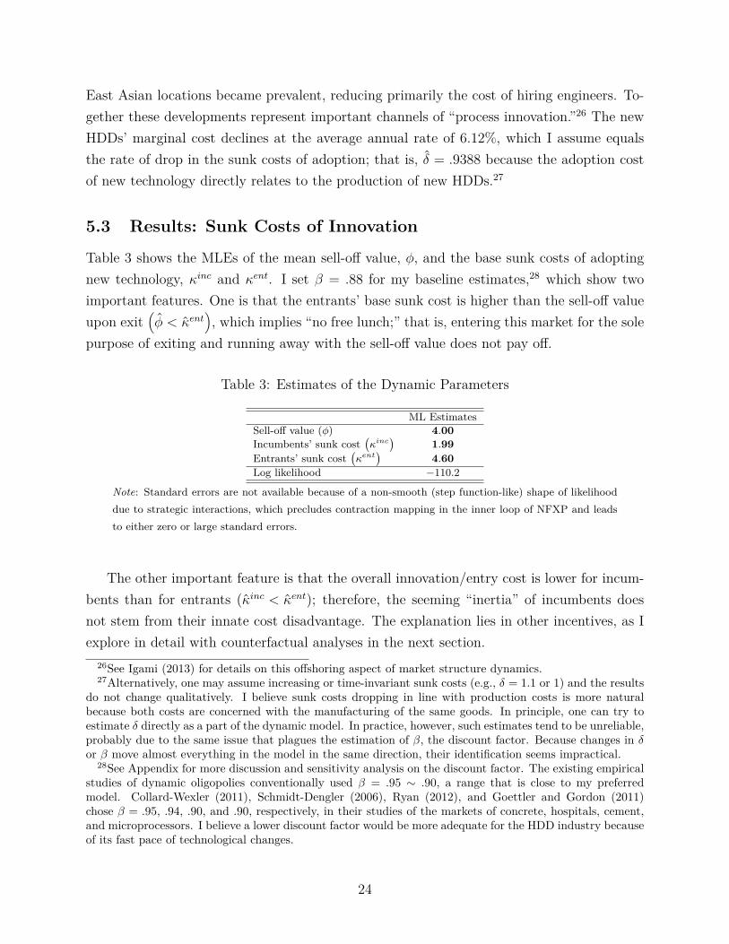
5.3 Results: Sunk Costs of Innovation

Table 3 shows the MLEs of the mean sell-off value, φ, and the base sunk costs of adoptingnew technology, κinc and κent. I set β = .88 for my baseline estimates,28 which show twoimportant features. One is that the entrants’ base sunk cost is higher than the sell-off valueupon exit

(φ < κent

), which implies “no free lunch;” that is, entering this market for the sole

purpose of exiting and running away with the sell-off value does not pay off.

Table 3: Estimates of the Dynamic Parameters

ML EstimatesSell-off value (φ) 4.00Incumbents’ sunk cost

(κinc

)1.99

Entrants’ sunk cost(κent

)4.60

Log likelihood −110.2

Note: Standard errors are not available because of a non-smooth (step function-like) shape of likelihooddue to strategic interactions, which precludes contraction mapping in the inner loop of NFXP and leadsto either zero or large standard errors.

The other important feature is that the overall innovation/entry cost is lower for incum-bents than for entrants (κinc < κent); therefore, the seeming “inertia” of incumbents doesnot stem from their innate cost disadvantage. The explanation lies in other incentives, as Iexplore in detail with counterfactual analyses in the next section.

26See Igami (2013) for details on this offshoring aspect of market structure dynamics.27Alternatively, one may assume increasing or time-invariant sunk costs (e.g., δ = 1.1 or 1) and the results

do not change qualitatively. I believe sunk costs dropping in line with production costs is more naturalbecause both costs are concerned with the manufacturing of the same goods. In principle, one can try toestimate δ directly as a part of the dynamic model. In practice, however, such estimates tend to be unreliable,probably due to the same issue that plagues the estimation of β, the discount factor. Because changes in δor β move almost everything in the model in the same direction, their identification seems impractical.

28See Appendix for more discussion and sensitivity analysis on the discount factor. The existing empiricalstudies of dynamic oligopolies conventionally used β = .95 ∼ .90, a range that is close to my preferredmodel. Collard-Wexler (2011), Schmidt-Dengler (2006), Ryan (2012), and Goettler and Gordon (2011)chose β = .95, .94, .90, and .90, respectively, in their studies of the markets of concrete, hospitals, cement,and microprocessors. I believe a lower discount factor would be more adequate for the HDD industry becauseof its fast pace of technological changes.

24

Two caveats are in order regarding the interpretations of innovation/entry cost estimates.First, κent embodies the costs of both entry and innovation for potential entrants, whereasκinc is strictly about incumbents’ innovation costs. Upon entry, entrants can always electto exit and recover φ, so that the truly “sunk” part of κent is κent − φ. Although the exactdecomposition of κent is conceptually infeasible, I am inclined to interpret the 0.60 (= κent−φ)part of κent as the pure “innovation” cost and the 4.00 (= φ) part as representing the “entry”fee. According to this interpretation, the meaning of κinc < κent becomes more nuanced; thatis, although incumbents may enjoy overall cost advantage over entrants, the latter might bebetter at innovation per se.29

Second, the result κinc < κent does not necessarily mean incumbents are entirely freefrom organizational, informational, or other disadvantages. Rather, my estimates simplysuggest incumbents enjoy a certain cost advantage over entrants in net terms. A possibleexplanation is that incumbents accumulate certain technological or marketing capabilitiesover the years, which outweigh other potential disadvantages associated with being largerand older.

Determining the exact contents of κinc and κent is beyond the scope of this paper, butincumbents’ overall cost advantage will have important welfare implications (see section 7).

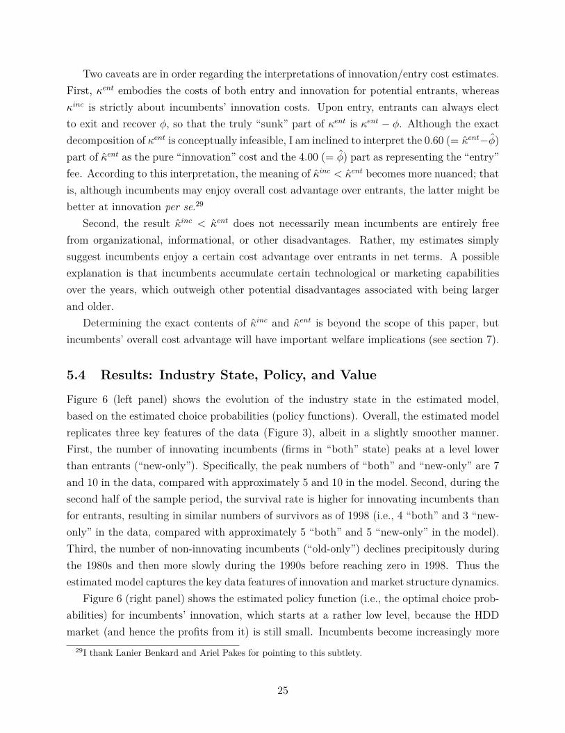
5.4 Results: Industry State, Policy, and Value

Figure 6 (left panel) shows the evolution of the industry state in the estimated model,based on the estimated choice probabilities (policy functions). Overall, the estimated modelreplicates three key features of the data (Figure 3), albeit in a slightly smoother manner.First, the number of innovating incumbents (firms in “both” state) peaks at a level lowerthan entrants (“new-only”). Specifically, the peak numbers of “both” and “new-only” are 7and 10 in the data, compared with approximately 5 and 10 in the model. Second, during thesecond half of the sample period, the survival rate is higher for innovating incumbents thanfor entrants, resulting in similar numbers of survivors as of 1998 (i.e., 4 “both” and 3 “new-only” in the data, compared with approximately 5 “both” and 5 “new-only” in the model).Third, the number of non-innovating incumbents (“old-only”) declines precipitously duringthe 1980s and then more slowly during the 1990s before reaching zero in 1998. Thus theestimated model captures the key data features of innovation and market structure dynamics.

Figure 6 (right panel) shows the estimated policy function (i.e., the optimal choice prob-abilities) for incumbents’ innovation, which starts at a rather low level, because the HDDmarket (and hence the profits from it) is still small. Incumbents become increasingly more

29I thank Lanier Benkard and Ariel Pakes for pointing to this subtlety.

25

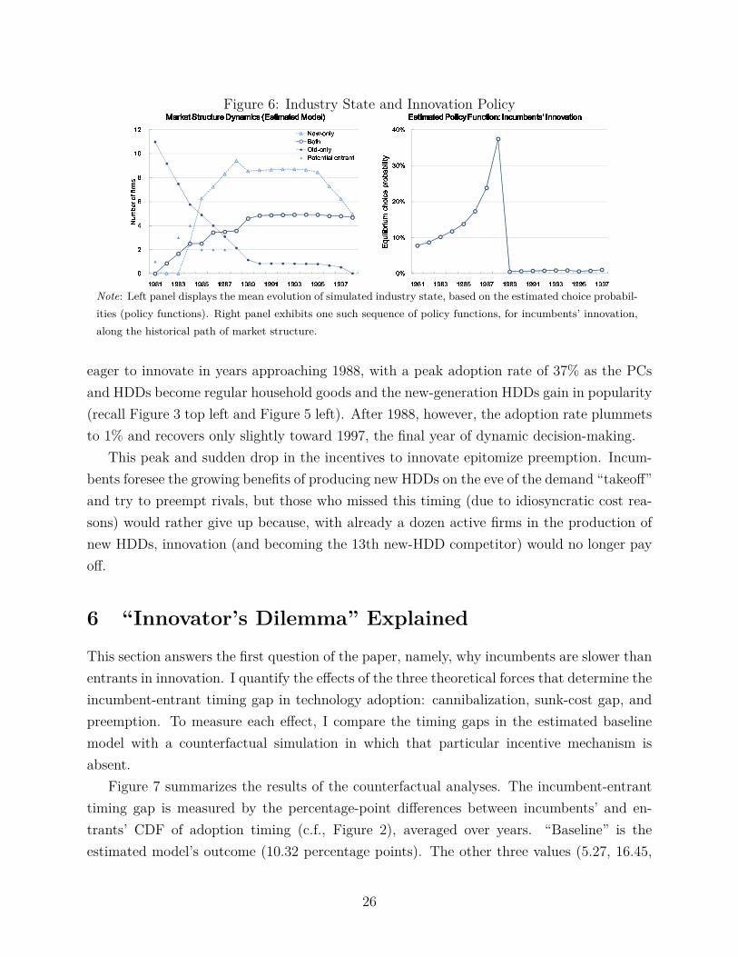
Figure 6: Industry State and Innovation Policy

�

�

�

�

�

� �

� �

� � � ��

� ��

�� ! " � #�$ � % & ' % � $ #�� ()��* ( � + ,�� ! " � #�$ � % & ' % � $ #�� ()��* ( � + ,�� ! " � #�$ � % & ' % � $ #�� ()��* ( � + ,�� ! " � #�$ � % & ' % � $ #�� ()��* ( � + ,- . / 0 1 2 3 45 1 6 78 3 9 0 1 2 3 4: 1 6 . 2 6 ; < 3 . 2 6 = < 2 6

� >

� � >

� � >

� � >

� � >

� � � �?� � � �� ?� � � ��

@ ABCDCE FC BGHI JC HKLFJE MECDCN O

' % � $ #)� � � ( P * + $ � ! Q � " � � $ * " R S " � � #�T � " � % U S " " * V � � $ * "' % � $ #)� � � ( P * + $ � ! Q � " � � $ * " R S " � � #�T � " � % U S " " * V � � $ * "' % � $ #)� � � ( P * + $ � ! Q � " � � $ * " R S " � � #�T � " � % U S " " * V � � $ * "' % � $ #)� � � ( P * + $ � ! Q � " � � $ * " R S " � � #�T � " � % U S " " * V � � $ * "

Note: Left panel displays the mean evolution of simulated industry state, based on the estimated choice probabil-ities (policy functions). Right panel exhibits one such sequence of policy functions, for incumbents’ innovation,along the historical path of market structure.

eager to innovate in years approaching 1988, with a peak adoption rate of 37% as the PCsand HDDs become regular household goods and the new-generation HDDs gain in popularity(recall Figure 3 top left and Figure 5 left). After 1988, however, the adoption rate plummetsto 1% and recovers only slightly toward 1997, the final year of dynamic decision-making.

This peak and sudden drop in the incentives to innovate epitomize preemption. Incum-bents foresee the growing benefits of producing new HDDs on the eve of the demand “takeoff”and try to preempt rivals, but those who missed this timing (due to idiosyncratic cost rea-sons) would rather give up because, with already a dozen active firms in the production ofnew HDDs, innovation (and becoming the 13th new-HDD competitor) would no longer payoff.

6 “Innovator’s Dilemma” Explained

This section answers the first question of the paper, namely, why incumbents are slower thanentrants in innovation. I quantify the effects of the three theoretical forces that determine theincumbent-entrant timing gap in technology adoption: cannibalization, sunk-cost gap, andpreemption. To measure each effect, I compare the timing gaps in the estimated baselinemodel with a counterfactual simulation in which that particular incentive mechanism isabsent.

Figure 7 summarizes the results of the counterfactual analyses. The incumbent-entranttiming gap is measured by the percentage-point differences between incumbents’ and en-trants’ CDF of adoption timing (c.f., Figure 2), averaged over years. “Baseline” is theestimated model’s outcome (10.32 percentage points). The other three values (5.27, 16.45,

26

and 51.73 percentage points) represent the simulated counterfactuals in which I “shut down”particular economic incentives.

Figure 7: Incumbents-Entrant Timing Gap in Innovation

�

��

��

��

��

� � ��

� ��

� �� ! ! "#� � $ ��

%&��! ' $ � !

� �� $ (��' $ )�� $ � �

*+$ � � !� !�� !+$ �-,/.�� $ ��+0+*21*+$ � � !� !�� !+$ �-,/.�� $ ��+0+*21*+$ � � !� !�� !+$ �-,/.�� $ ��+0+*21*+$ � � !� !�� !+$ �-,/.�� $ ��+0+*21/3 ��!� ��!�� !+��$ � � ��43 ��!� ��!�� !+��$ � � ��43 ��!� ��!�� !+��$ � � ��43 ��!� ��!�� !+��$ � � ��4

Note: * outside the graph range. Timing gap is measured by the percentage-point difference betweenincumbents’ and entrants’ CDF of adoption timing, averaged over years during the first half of thesample period. “Baseline” outcome is based on the estimated model (see previous section), whereasthe other three are the counterfactual simulation results, which I explain in detail in this section.

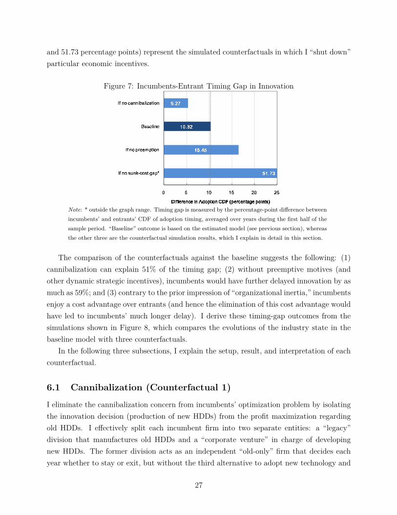
The comparison of the counterfactuals against the baseline suggests the following: (1)cannibalization can explain 51% of the timing gap; (2) without preemptive motives (andother dynamic strategic incentives), incumbents would have further delayed innovation by asmuch as 59%; and (3) contrary to the prior impression of “organizational inertia,” incumbentsenjoy a cost advantage over entrants (and hence the elimination of this cost advantage wouldhave led to incumbents’ much longer delay). I derive these timing-gap outcomes from thesimulations shown in Figure 8, which compares the evolutions of the industry state in thebaseline model with three counterfactuals.

In the following three subsections, I explain the setup, result, and interpretation of eachcounterfactual.

6.1 Cannibalization (Counterfactual 1)

I eliminate the cannibalization concern from incumbents’ optimization problem by isolatingthe innovation decision (production of new HDDs) from the profit maximization regardingold HDDs. I effectively split each incumbent firm into two separate entities: a “legacy”division that manufactures old HDDs and a “corporate venture” in charge of developingnew HDDs. The former division acts as an independent “old-only” firm that decides eachyear whether to stay or exit, but without the third alternative to adopt new technology and

27

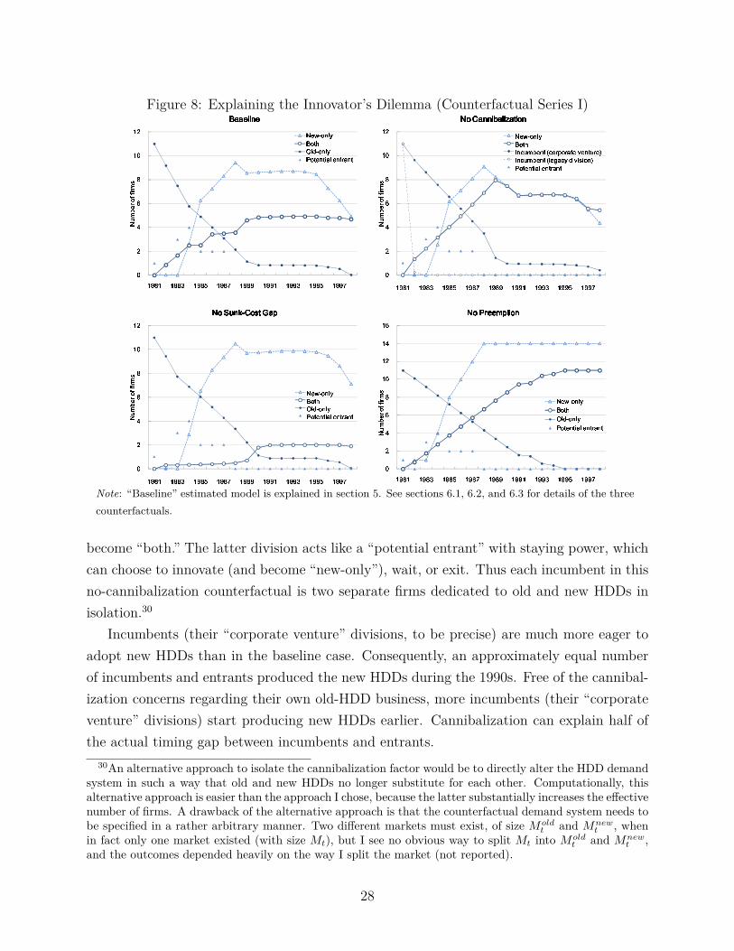
Figure 8: Explaining the Innovator’s Dilemma (Counterfactual Series I)

�

�

�

�

�

� �

� �

� � � ��

� ��

� � � � � � � ��

� � � ! " # $% ! & '( # ) ! " # $* ! & � " & + , # � " & - , " &

�

�

�

�

�

� �

� �

� � � �.� � � ��

� ��

/ 0 1 � � � � 2 � � � 3 � 4 � 0 �/ 0 1 � � � � 2 � � � 3 � 4 � 0 �/ 0 1 � � � � 2 � � � 3 � 4 � 0 �/ 0 1 � � � � 2 � � � 3 � 4 � 0 �

� � � ! " # $% ! & '5 " 6 7 8 9 � " & : 6 ! - ; ! - , & � < � " & 7 - � =5 " 6 7 8 9 � " & : # � > , 6 $ ) + < + ? + ! " =* ! & � " & + , # � " & - , " &

�

�

�

�

�

� �

� �

� � � ��

� ��

/ 0 @ A � B/ 0 @ A � B/ 0 @ A � B/ 0 @ A � B CC CC 1 0 � 4 DE� F1 0 � 4 DE� F1 0 � 4 DE� F1 0 � 4 DE� F

� � � ! " # $% ! & '( # ) ! " # $* ! & � " & + , # � " & - , " &

�

�

�

�

�

� �

� �

� �

� �

� � � �.� � � ��

� ��

/ 0EG H � � IJF 4 � 0 �/ 0EG H � � IJF 4 � 0 �/ 0EG H � � IJF 4 � 0 �/ 0EG H � � IJF 4 � 0 �

� � � ! " # $% ! & '( # ) ! " # $* ! & � " & + , # � " & - , " &

Note: “Baseline” estimated model is explained in section 5. See sections 6.1, 6.2, and 6.3 for details of the threecounterfactuals.

become “both.” The latter division acts like a “potential entrant” with staying power, whichcan choose to innovate (and become “new-only”), wait, or exit. Thus each incumbent in thisno-cannibalization counterfactual is two separate firms dedicated to old and new HDDs inisolation.30

Incumbents (their “corporate venture” divisions, to be precise) are much more eager toadopt new HDDs than in the baseline case. Consequently, an approximately equal numberof incumbents and entrants produced the new HDDs during the 1990s. Free of the cannibal-ization concerns regarding their own old-HDD business, more incumbents (their “corporateventure” divisions) start producing new HDDs earlier. Cannibalization can explain half ofthe actual timing gap between incumbents and entrants.

30An alternative approach to isolate the cannibalization factor would be to directly alter the HDD demandsystem in such a way that old and new HDDs no longer substitute for each other. Computationally, thisalternative approach is easier than the approach I chose, because the latter substantially increases the effectivenumber of firms. A drawback of the alternative approach is that the counterfactual demand system needs tobe specified in a rather arbitrary manner. Two different markets must exist, of size Mold

t and Mnewt , when

in fact only one market existed (with size Mt), but I see no obvious way to split Mt into Moldt and Mnew

t ,and the outcomes depended heavily on the way I split the market (not reported).

28

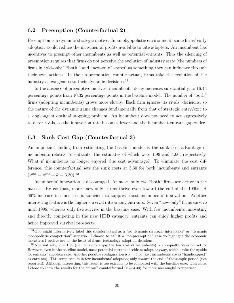
6.2 Preemption (Counterfactual 2)

Preemption is a dynamic strategic motive. In an oligopolistic environment, some firms’ earlyadoption would reduce the incremental profits available to late adopters. An incumbent hasincentives to preempt other incumbents as well as potential entrants. Thus the silencing ofpreemption requires that firms do not perceive the evolution of industry state (the numbers offirms in “old-only,” “both,” and “new-only” states) as something they can influence throughtheir own actions. In the no-preemption counterfactual, firms take the evolution of theindustry as exogenous to their dynamic decisions.31

In the absence of preemptive motives, incumbents’ delay increases substantially, to 16.45percentage points from 10.32 percentage points in the baseline model. The number of “both”firms (adopting incumbents) grows more slowly. Each firm ignores its rivals’ decisions, sothe nature of the dynamic game changes fundamentally from that of strategic entry/exit toa single-agent optimal stopping problem. An incumbent does not need to act aggressivelyto deter rivals, so the innovation rate becomes lower and the incumbent-entrant gap wider.

6.3 Sunk Cost Gap (Counterfactual 3)

An important finding from estimating the baseline model is the sunk cost advantage ofincumbents relative to entrants, the estimates of which were 1.99 and 4.60, respectively.What if incumbents no longer enjoyed this cost advantage? To eliminate the cost dif-ference, this counterfactual sets the sunk costs at 3.30 for both incumbents and entrants(κinc = κent = κ = 3.30).32

Incumbents’ innovation is discouraged. At most, only two “both” firms are active in themarket. By contrast, more “new-only” firms thrive even toward the end of the 1990s. A66% increase in sunk cost is sufficient to suppress most incumbents’ innovation. Anotherinteresting feature is the higher survival rate among entrants. Seven “new-only” firms surviveuntil 1998, whereas only five survive in the baseline case. With few incumbents innovatingand directly competing in the new HDD category, entrants can enjoy higher profits andhence improved survival prospects.

31One might alternatively label this counterfactual as a “no dynamic strategic interaction” or “dynamicmonopolistic competition” scenario. I choose to call it a “no-preemption” case to highlight the economicincentives I believe are at the heart of firms’ technology adoption decisions.

32Alternatively, κ = 1.99 (i.e., entrants enjoy the low cost of incumbents) is an equally plausible setup.However, even in the baseline model, most potential entrants decide to adopt anyway, which limits the upsidefor entrants’ adoption rate. Another possible configuration is κ = 4.60 (i.e., incumbents are as “handicapped”as entrants). This setup results in few incumbents’ adoption, only toward the end of the sample period (notreported). Although interesting, this result is too extreme to be compared with the baseline case. Therefore,I chose to show the results for the “mean” counterfactual (κ = 3.30) for more meaningful comparison.

29

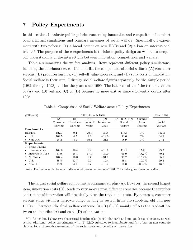
7 Policy Experiments

In this section, I evaluate public policies concerning innovation and competition. I conductcounterfactual simulations and compare measures of social welfare. Specifically, I experi-ment with two policies: (1) a broad patent on new HDDs and (2) a ban on internationaltrade.33 The purpose of these experiments is to inform policy design as well as to deepenour understanding of the interactions between innovation, competition, and welfare.

Table 4 summarizes the welfare analysis. Rows represent different policy simulations,including the benchmark cases. Columns list the components of social welfare: (A) consumersurplus, (B) producer surplus, (C) sell-off value upon exit, and (D) sunk costs of innovation.Social welfare is their sum. I display social welfare figures separately for the sample period(1981 through 1998) and for the years since 1999. The latter consists of the terminal valuesof (A) and (B) but not (C) or (D) because no more exit or innovation/entry occurs after1998.

Table 4: Comparison of Social Welfare across Policy Experiments

(Billion $) 1981 through 1998 From 1999(A) (B) (C) (D) (A+B+C+D) Change

Consumer Producer Sell-Off Innovation Social from SocialSurplus Surplus Value Cost Welfare Baseline Welfare

BenchmarksBaseline 127.7 9.4 20.0 −39.5 117.6 0% 112.3• U.S. 102.5 4.5 9.6 −18.0 98.6 0% 84.9• Non U.S. 25.2 4.9 10.4 −21.6 18.9 0% 27.4Experiments1. Broad Patent• Pre-announced 109.6 16.4 6.2 −13.9 118.2 0.5% 99.5• Surprise in 1988 67.9 15.1 17.0 −39.0 61.0 −48.2% 30.42. No Trade 107.4 16.8 6.7 −31.1 99.7 −15.2% 95.5• U.S. 88.5 12.7 0.0 −12.4 88.8 −10.0% 79.4• Non U.S. 18.9 4.1 6.7 −18.7 11.0 −88.9% 16.2

Note: Each number is the sum of discounted present values as of 1981. * Includes government subsidies.

The largest social welfare component is consumer surplus (A). However, the second largestitem, innovation costs (D), tends to vary most across different scenarios because the numberand timing of innovation will drastically alter the total sunk costs. By contrast, consumersurplus stays within a narrower range as long as several firms are supplying old and newHDDs. Therefore, the final welfare outcome (A+B+C+D) mainly reflects the tradeoff be-tween the benefits (A) and costs (D) of innovation.

33In Appendix, I show two theoretical benchmarks (social planner’s and monopolist’s solutions), as wellas two additional policy experiments with (3) R&D subsidies to incumbents and (4) a ban on non-competeclauses, for a thorough assessment of the social costs and benefits of innovation.

30

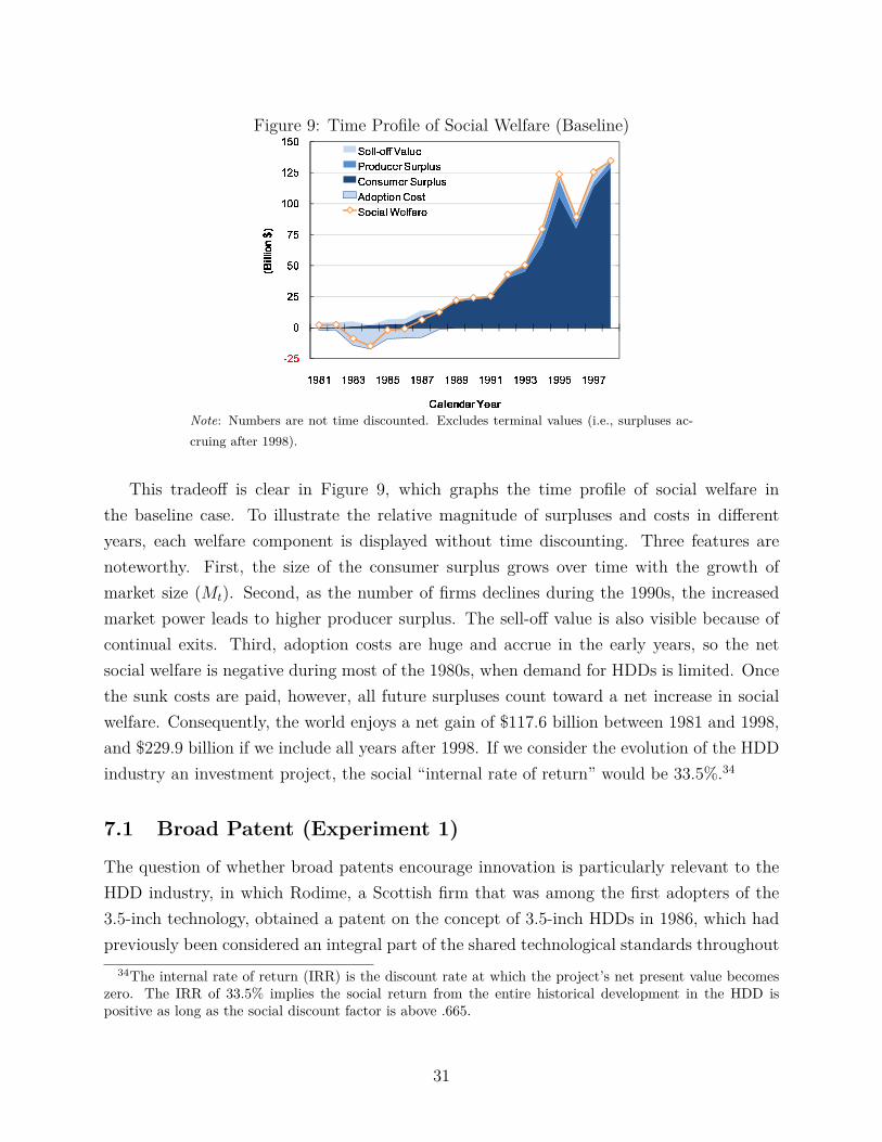
Figure 9: Time Profile of Social Welfare (Baseline)

�

� ��

�

��

��

� �

��

��

��

��

��

��

��

��

�� !� �� !� ��

"#�� $ % % & �� '��(#� $ ��'�)*��+",'�� -�� '�.� $ ��.*'�/��*"#'�� -�� '�.01� $ - 2 3 $ �4� $ . 2" $ )+3 �� 56�� % ��

Note: Numbers are not time discounted. Excludes terminal values (i.e., surpluses ac-cruing after 1998).

This tradeoff is clear in Figure 9, which graphs the time profile of social welfare inthe baseline case. To illustrate the relative magnitude of surpluses and costs in differentyears, each welfare component is displayed without time discounting. Three features arenoteworthy. First, the size of the consumer surplus grows over time with the growth ofmarket size (Mt). Second, as the number of firms declines during the 1990s, the increasedmarket power leads to higher producer surplus. The sell-off value is also visible because ofcontinual exits. Third, adoption costs are huge and accrue in the early years, so the netsocial welfare is negative during most of the 1980s, when demand for HDDs is limited. Oncethe sunk costs are paid, however, all future surpluses count toward a net increase in socialwelfare. Consequently, the world enjoys a net gain of $117.6 billion between 1981 and 1998,and $229.9 billion if we include all years after 1998. If we consider the evolution of the HDDindustry an investment project, the social “internal rate of return” would be 33.5%.34

7.1 Broad Patent (Experiment 1)

The question of whether broad patents encourage innovation is particularly relevant to theHDD industry, in which Rodime, a Scottish firm that was among the first adopters of the3.5-inch technology, obtained a patent on the concept of 3.5-inch HDDs in 1986, which hadpreviously been considered an integral part of the shared technological standards throughout

34The internal rate of return (IRR) is the discount rate at which the project’s net present value becomeszero. The IRR of 33.5% implies the social return from the entire historical development in the HDD ispositive as long as the social discount factor is above .665.

31

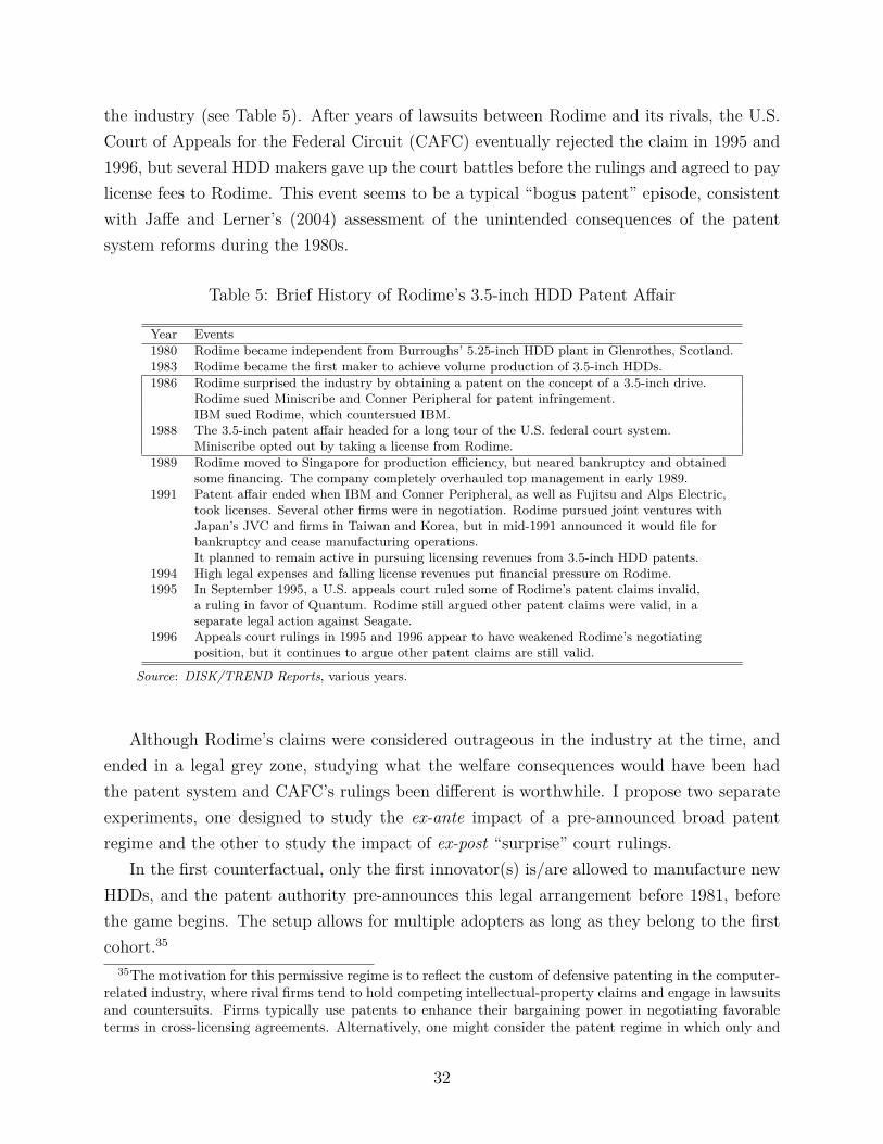
the industry (see Table 5). After years of lawsuits between Rodime and its rivals, the U.S.Court of Appeals for the Federal Circuit (CAFC) eventually rejected the claim in 1995 and1996, but several HDD makers gave up the court battles before the rulings and agreed to paylicense fees to Rodime. This event seems to be a typical “bogus patent” episode, consistentwith Jaffe and Lerner’s (2004) assessment of the unintended consequences of the patentsystem reforms during the 1980s.

Table 5: Brief History of Rodime’s 3.5-inch HDD Patent Affair

Year Events1980 Rodime became independent from Burroughs’ 5.25-inch HDD plant in Glenrothes, Scotland.1983 Rodime became the first maker to achieve volume production of 3.5-inch HDDs.1986 Rodime surprised the industry by obtaining a patent on the concept of a 3.5-inch drive.

Rodime sued Miniscribe and Conner Peripheral for patent infringement.IBM sued Rodime, which countersued IBM.

1988 The 3.5-inch patent affair headed for a long tour of the U.S. federal court system.Miniscribe opted out by taking a license from Rodime.

1989 Rodime moved to Singapore for production efficiency, but neared bankruptcy and obtainedsome financing. The company completely overhauled top management in early 1989.

1991 Patent affair ended when IBM and Conner Peripheral, as well as Fujitsu and Alps Electric,took licenses. Several other firms were in negotiation. Rodime pursued joint ventures withJapan’s JVC and firms in Taiwan and Korea, but in mid-1991 announced it would file forbankruptcy and cease manufacturing operations.It planned to remain active in pursuing licensing revenues from 3.5-inch HDD patents.

1994 High legal expenses and falling license revenues put financial pressure on Rodime.1995 In September 1995, a U.S. appeals court ruled some of Rodime’s patent claims invalid,

a ruling in favor of Quantum. Rodime still argued other patent claims were valid, in aseparate legal action against Seagate.

1996 Appeals court rulings in 1995 and 1996 appear to have weakened Rodime’s negotiatingposition, but it continues to argue other patent claims are still valid.

Source: DISK/TREND Reports, various years.

Although Rodime’s claims were considered outrageous in the industry at the time, andended in a legal grey zone, studying what the welfare consequences would have been hadthe patent system and CAFC’s rulings been different is worthwhile. I propose two separateexperiments, one designed to study the ex-ante impact of a pre-announced broad patentregime and the other to study the impact of ex-post “surprise” court rulings.

In the first counterfactual, only the first innovator(s) is/are allowed to manufacture newHDDs, and the patent authority pre-announces this legal arrangement before 1981, beforethe game begins. The setup allows for multiple adopters as long as they belong to the firstcohort.35

35The motivation for this permissive regime is to reflect the custom of defensive patenting in the computer-related industry, where rival firms tend to hold competing intellectual-property claims and engage in lawsuitsand countersuits. Firms typically use patents to enhance their bargaining power in negotiating favorableterms in cross-licensing agreements. Alternatively, one might consider the patent regime in which only and

32

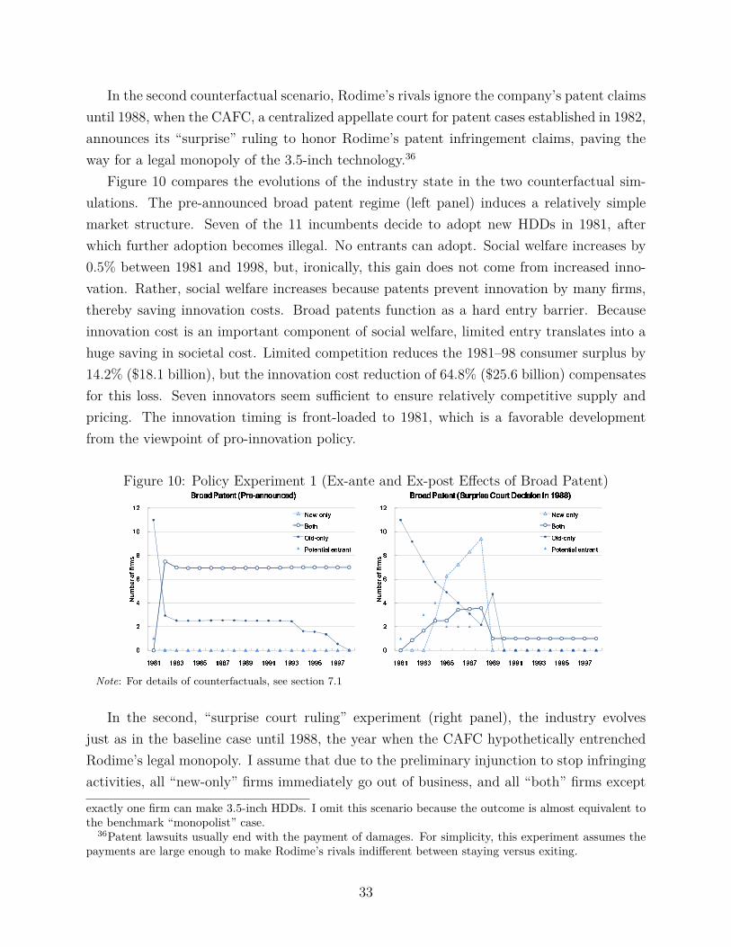
In the second counterfactual scenario, Rodime’s rivals ignore the company’s patent claimsuntil 1988, when the CAFC, a centralized appellate court for patent cases established in 1982,announces its “surprise” ruling to honor Rodime’s patent infringement claims, paving theway for a legal monopoly of the 3.5-inch technology.36

Figure 10 compares the evolutions of the industry state in the two counterfactual sim-ulations. The pre-announced broad patent regime (left panel) induces a relatively simplemarket structure. Seven of the 11 incumbents decide to adopt new HDDs in 1981, afterwhich further adoption becomes illegal. No entrants can adopt. Social welfare increases by0.5% between 1981 and 1998, but, ironically, this gain does not come from increased inno-vation. Rather, social welfare increases because patents prevent innovation by many firms,thereby saving innovation costs. Broad patents function as a hard entry barrier. Becauseinnovation cost is an important component of social welfare, limited entry translates into ahuge saving in societal cost. Limited competition reduces the 1981–98 consumer surplus by14.2% ($18.1 billion), but the innovation cost reduction of 64.8% ($25.6 billion) compensatesfor this loss. Seven innovators seem sufficient to ensure relatively competitive supply andpricing. The innovation timing is front-loaded to 1981, which is a favorable developmentfrom the viewpoint of pro-innovation policy.

Figure 10: Policy Experiment 1 (Ex-ante and Ex-post Effects of Broad Patent)

�

�

�

�

�

� �

� �

� � � ��

� ��

� � � � � � � � � � � � � � �� ! � " � � #� � � � ! � " � � #� � � � ! � " � � #� � � � ! � " � � #

$ % & ' ( ) * +, ( - ./ * 0 ' ( ) * +1 ( - % ) - 2 3 * % ) - 4 3 ) -

�

�

�

�

�

� �

� �

� � � �5� � � ��

� ��

� � � � � � � � � � � � 6 ! � 7 � 8 9 � : � ! � � ; � " 8 9 8 � � 8 �=< > ? ? #� � � � � � � � � � � � 6 ! � 7 � 8 9 � : � ! � � ; � " 8 9 8 � � 8 �=< > ? ? #� � � � � � � � � � � � 6 ! � 7 � 8 9 � : � ! � � ; � " 8 9 8 � � 8 �=< > ? ? #� � � � � � � � � � � � 6 ! � 7 � 8 9 � : � ! � � ; � " 8 9 8 � � 8 �=< > ? ? #

$ % & ' ( ) * +, ( - ./ * 0 ' ( ) * +1 ( - % ) - 2 3 * % ) - 4 3 ) -

Note: For details of counterfactuals, see section 7.1

In the second, “surprise court ruling” experiment (right panel), the industry evolvesjust as in the baseline case until 1988, the year when the CAFC hypothetically entrenchedRodime’s legal monopoly. I assume that due to the preliminary injunction to stop infringingactivities, all “new-only” firms immediately go out of business, and all “both” firms except

exactly one firm can make 3.5-inch HDDs. I omit this scenario because the outcome is almost equivalent tothe benchmark “monopolist” case.

36Patent lawsuits usually end with the payment of damages. For simplicity, this experiment assumes thepayments are large enough to make Rodime’s rivals indifferent between staying versus exiting.

33

Rodime are forced back to “old-only” status by 1989, a position that is so unattractivethe firms all subsequently elect to exit the industry. In stark contrast with the previousexperiment, social welfare drops by 48.2% in the ex-post patent scenario because most firmshad already paid the sunk costs and started production of 3.5-inch HDDs by 1988, so that nocost saving exists as in the “pre-announced” patent regime. Instead, the only major changeis that the industry becomes a monopoly from 1990 and consumers thus suffer.

In the existing literature, Lerner (1994) found a positive correlation between broaderpatents and increased innovative activities, whereas Sakakibara and Branstetter (2001) foundno measurable relationship. By contrast, the results of my experiments point to the possi-bility that allowing for broad patents might decrease innovative activities. These divergingresults are not necessarily at odds with each other, for two reasons. First, even when thenumber of total innovators decreases in the long run, if the timing is earlier, the numberof innovators will be higher in the short run. In other words, a tradeoff seems to existbetween short- and long-run levels of innovative activities, and patents may change this bal-ance. These changes in the timing and number of innovations embody the ex-ante effect ofpatents. Second, because patents are legal monopoly rights by definition, if one firm’s patenton a particular product/technology is strictly honored and protected, rival firms must be ex-cluded from the same product/technology. The second experiment highlights this ex-posteffect of broad patents.

7.2 No International Trade (Experiment 2)

Disputes over intellectual property rights often become international trade disputes in thecomputer-related industries. For example, Apple sued HTC, a leading manufacturer of theAndroid-based smart phone in Taiwan, in July 2011 for two patent infringement claimsrelated to touch-screen technologies in iPhones. HTC countersued Apple, but, meanwhile,the U.S. Commerce Department started contemplating banning U.S. imports of HTC’s smartphones. A similar dispute between Apple and Sumsung led to a temporary ban on Samsung’sGalaxy tablet computer in Germany and Australia. Given the global nature of competitionin these high-tech industries, intellectual property and competition policy issues tend tobecome international trade issues at the same time. Although the international trade ofHDDs avoided political interventions during the sample period, other sectors of the computerindustry were full of trade disputes.37 Because the HDD industry data are relatively freefrom political complications, they provide a clean laboratory in which to experiment with

37For example, Japan’s Ministry of International Trade and Commerce restricted the imports and manu-facturing of IBM’s computers during the 1960s. The U.S. Commerce Department imposed “anti-dumping”duties on Samsung’s memory chips (DRAM) in the early 1990s.

34

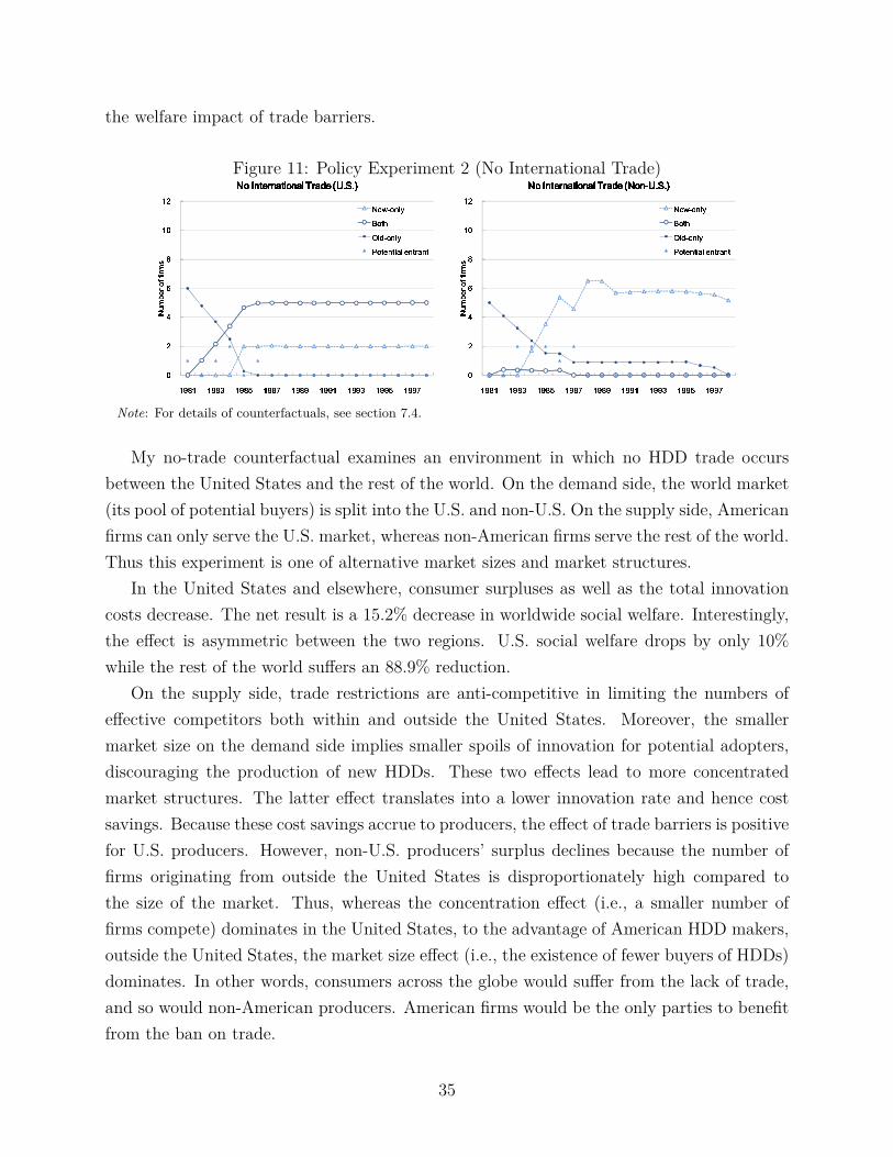
the welfare impact of trade barriers.

Figure 11: Policy Experiment 2 (No International Trade)

�

�

�

�

�

� �

� �

� � � ��

� ��

� �� ! � � " � # $ % & % '� �� ! � � " � # $ % & % '� �� ! � � " � # $ % & % '� �� ! � � " � # $ % & % '

( ) * + , - . /0 , 1 23 . 4 + , - . /5 , 1 ) - 1 6 7 . ) - 1 8 7 - 1

�

�

�

�

�

� �

� �

� � � �9� � � ��

� ��

� �� ! � � " � # � � �� ! � � " � # � � �� ! � � " � # � � �� ! � � " � # � � � :: :: $ % & % '$ % & % '$ % & % '$ % & % '

( ) * + , - . /0 , 1 23 . 4 + , - . /5 , 1 ) - 1 6 7 . ) - 1 8 7 - 1

Note: For details of counterfactuals, see section 7.4.

My no-trade counterfactual examines an environment in which no HDD trade occursbetween the United States and the rest of the world. On the demand side, the world market(its pool of potential buyers) is split into the U.S. and non-U.S. On the supply side, Americanfirms can only serve the U.S. market, whereas non-American firms serve the rest of the world.Thus this experiment is one of alternative market sizes and market structures.

In the United States and elsewhere, consumer surpluses as well as the total innovationcosts decrease. The net result is a 15.2% decrease in worldwide social welfare. Interestingly,the effect is asymmetric between the two regions. U.S. social welfare drops by only 10%while the rest of the world suffers an 88.9% reduction.

On the supply side, trade restrictions are anti-competitive in limiting the numbers ofeffective competitors both within and outside the United States. Moreover, the smallermarket size on the demand side implies smaller spoils of innovation for potential adopters,discouraging the production of new HDDs. These two effects lead to more concentratedmarket structures. The latter effect translates into a lower innovation rate and hence costsavings. Because these cost savings accrue to producers, the effect of trade barriers is positivefor U.S. producers. However, non-U.S. producers’ surplus declines because the number offirms originating from outside the United States is disproportionately high compared tothe size of the market. Thus, whereas the concentration effect (i.e., a smaller number offirms compete) dominates in the United States, to the advantage of American HDD makers,outside the United States, the market size effect (i.e., the existence of fewer buyers of HDDs)dominates. In other words, consumers across the globe would suffer from the lack of trade,and so would non-American producers. American firms would be the only parties to benefitfrom the ban on trade.

35

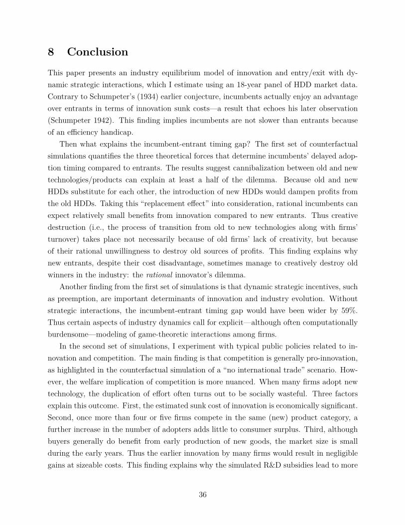
8 Conclusion

This paper presents an industry equilibrium model of innovation and entry/exit with dy-namic strategic interactions, which I estimate using an 18-year panel of HDD market data.Contrary to Schumpeter’s (1934) earlier conjecture, incumbents actually enjoy an advantageover entrants in terms of innovation sunk costs—a result that echoes his later observation(Schumpeter 1942). This finding implies incumbents are not slower than entrants becauseof an efficiency handicap.

Then what explains the incumbent-entrant timing gap? The first set of counterfactualsimulations quantifies the three theoretical forces that determine incumbents’ delayed adop-tion timing compared to entrants. The results suggest cannibalization between old and newtechnologies/products can explain at least a half of the dilemma. Because old and newHDDs substitute for each other, the introduction of new HDDs would dampen profits fromthe old HDDs. Taking this “replacement effect” into consideration, rational incumbents canexpect relatively small benefits from innovation compared to new entrants. Thus creativedestruction (i.e., the process of transition from old to new technologies along with firms’turnover) takes place not necessarily because of old firms’ lack of creativity, but becauseof their rational unwillingness to destroy old sources of profits. This finding explains whynew entrants, despite their cost disadvantage, sometimes manage to creatively destroy oldwinners in the industry: the rational innovator’s dilemma.

Another finding from the first set of simulations is that dynamic strategic incentives, suchas preemption, are important determinants of innovation and industry evolution. Withoutstrategic interactions, the incumbent-entrant timing gap would have been wider by 59%.Thus certain aspects of industry dynamics call for explicit—although often computationallyburdensome—modeling of game-theoretic interactions among firms.

In the second set of simulations, I experiment with typical public policies related to in-novation and competition. The main finding is that competition is generally pro-innovation,as highlighted in the counterfactual simulation of a “no international trade” scenario. How-ever, the welfare implication of competition is more nuanced. When many firms adopt newtechnology, the duplication of effort often turns out to be socially wasteful. Three factorsexplain this outcome. First, the estimated sunk cost of innovation is economically significant.Second, once more than four or five firms compete in the same (new) product category, afurther increase in the number of adopters adds little to consumer surplus. Third, althoughbuyers generally do benefit from early production of new goods, the market size is smallduring the early years. Thus the earlier innovation by many firms would result in negligiblegains at sizeable costs. This finding explains why the simulated R&D subsidies lead to more

36

innovation but reduced social welfare, and also why a (pre-announced) broad-based patent,which represents a fairly anti-competitive intellectual property regime, results in increasedsocial welfare.

Overall, the historical welfare performance of the HDD industry in the data seems dif-ficult to beat, even with carefully designed policy interventions, so Schumpeter (1942) wasprobably right when he observed the world economy was benefiting from an approximatelysufficient amount of competition and innovation. Although some of these results would bespecific to the HDD market, the economic incentives studied here are general and could beexpected to operate in many oligopolistic markets. Similar trajectories of creative destruc-tion are also widely observed across industries, especially in computer-related sectors. Theseconsiderations lead me to believe this paper’s analytical framework, as well as its empir-ical findings, could be applicable elsewhere: old winners can survive the “gale of creativedestruction” only through creative self -destruction.

37

Appendix

A.1 Regressing Innovation Timing on Firm Characteristics

As a preliminary, descriptive analysis, I regress the timing of innovation (i.e., each firm’syear of initial shipment of new-generation HDDs) on firm characteristics. Table 6 reports theestimation results based on a standard duration model (Cox proportional hazard estimates).The estimates suggest incumbents are 50% less likely than entrants to innovate in a givenyear, even after controlling for all of the observed characteristics.

Table 6: Preliminary Regression of Innovation Timing on Firm Characteristics

Duration model (Cox proportional hazard estimates)Dependent variable: Decision to Innovate (1) (2) (3)

Firm characteristicsIncumbent .41∗∗∗ (.06) .53∗∗∗ (.09) .50∗∗∗ (.09)Initial generation of entry5.25-inch − (−) .84 (.18) .71 (.19)3.5-inch − (−) .52∗∗∗ (.12) .46∗∗∗ (.12)2.5-inch − (−) .34∗∗∗ (.10) .91 (.40)Organizational FormSpecialized HDD start-up − (−) 1.04 (.22) 1.01 (.22)Computer maker (“backward” integration) − (−) 1.39 (.29) 1.32 (.28)HDD component maker (“forward” integration) − (−) .55 (.21) .54∗ (.20)Region of OriginU.S. − (−) 1.04 (.32) 1.18 (.37)Asia − (−) 1.91∗∗ (.58) 1.90∗∗ (.58)Europe (West) − (−) 1.01 (.37) 1.20 (.45)Europe (East) − (−) .14∗ (.15) .16∗ (.17)Industry stateNumber of firms − (−) − (−) 1.16∗∗∗ (.05)Number of firms squared − (−) − (−) .99∗∗∗ (.00)Number of subjects (firms) 437 437 437Number of innovations 190 190 190Time at risk of innovation 2, 591 2, 591 2, 591Number of observations 1, 842 1, 842 1, 842Log likelihood −1, 018 −997 −990

Note: Coefficients greater (less) than 1 indicate higher (lower) propensities to innovate. Omitted categories are“Potential entrant,” “8-inch,” “Other electronics maker (horizontal diversification),” and “Brazil.” ***, **, and* indicate signifiance at the 1%, 5%, and 10% levels, respectively. Standard errors in parentheses.

I employ two different definitions of entrants in these regressions. The first definitionis data-driven and narrower: a potential entrant is recognized when a new firm announcesthe product specifications without actually manufacturing or shipping them. The seconddefinition is more conceptually motivated and broader: for all of the potential entrants thatannounced or shipped HDDs, I count as “time at risk (of innovation)” all years since theindustry-wide establishment of new-generation standards. That is, regardless of whether

38

these new firms were already incorporated or not, I pretend that their founders were con-sidering the innovation and entry, from the moment the industry consensus emerged on thephysical size of new-generation HDDs.

Econometrically, regressions based on the first definition would over-estimate the en-trants’ propensity to innovate because this definition recognizes entrants only when theywere most serious about innovation. In contrast, regressions based on the second definitionwould under-estimate entrants’ propensity to innovate because all years until actual ship-ments are interpreted as evidence against their innovativeness, regardless of whether theyexisted as firms or not. Table 6 reports only the results based on the second definition, inorder to show that entrants were twice more likely to innovate than incumbents, even whenI use the definition that would bias against such findings.

A.2 Likelihood Function

The contributions of the other three types of firms are

f both (dit|st; φ) = prboth (dit = exit)I(dit=exit) prboth (dit = stay)I(dit=stay) ,

fnew (dit|st; φ) = prnew (dit = exit)I(dit=exit) prnew (dit = stay)I(dit=stay) , and

fpe(dit|st; κent, δ

)= prpe (dit = quit)I(dit=quit) prpe (dit = adopt)I(dit=adopt) ,

where

prboth (dit = exit) = exp (φ)exp (φ) + exp

(EεV both

t+1 (st+1)) ,

prboth (dit = stay) =exp

(EεV

botht+1 (st+1)

)exp (φ) + exp

(EεV both

t+1 (st+1)) ,

prnew (dit = exit) = exp (φ)exp (φ) + exp (EεV new

t+1 (st+1)),

prnew (dit = stay) =exp

(EεV

newt+1 (st+1)

)exp (φ) + exp (EεV new

t+1 (st+1)),

prpe (dit = quit) = exp (0)exp (0) + exp (EεV new

t+1 (st+1) − δtκent), and

prpe (dit = adopt) =exp

(EεV

newt+1 (st+1) − δtκent

)exp (0) + exp (EεV new

t+1 (st+1) − δtκent).

39

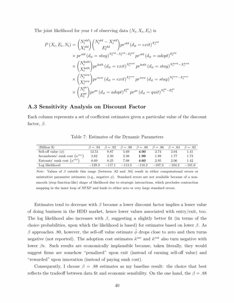
The joint likelihood for year t of observing data (Nt, Xt, Et) is

P (Xt, Et, Nt) =(

N oldt

Xoldt

)(N old

t − Xoldt

Eoldt

)prold (dit = exit)Xold

t

× prold (dit = stay)Noldt −Xold

t −Eoldt prold (dit = adopt)Eold

t

×(

N botht

Xbotht

)prboth (dit = exit)Xboth

t prboth (dit = stay)Nbotht −Xboth

t

×(

Nnewt

Xnewt

)prnew (dit = exit)Xnew

t prnew (dit = stay)Nnewt −Xnew

t

×(

Npet

Epet

)prpe (dit = adopt)Epe

t prpe (dit = quit)Npet −Epe

t

A.3 Sensitivity Analysis on Discount Factor

Each column represents a set of coefficient estimates given a particular value of the discountfactor, β.

Table 7: Estimates of the Dynamic Parameters

(Billion $) β = .94 β = .92 β = .90 β = .88 β = .86 β = .84 β = .82Sell-off value (φ) 12.51 8.87 5.69 4.00 2.74 2.04 1.41Incumbents’ sunk cost

(κinc

)2.62 2.50 2.38 1.99 1.89 1.77 1.72

Entrants’ sunk cost(κent

)8.69 8.25 7.08 4.60 2.95 2.06 1.42

Log likelihood −129.3 −117.1 −113.3 −110.2 −107.3 −104.2 −101.6

Note: Values of β outside this range (between .82 and .94) result in either computational errors orunintuitive parameter estimates (e.g., negative φ). Standard errors are not available because of a non-smooth (step function-like) shape of likelihood due to strategic interactions, which precludes contractionmapping in the inner loop of NFXP and leads to either zero or very large standard errors.

Estimates tend to decrease with β because a lower discount factor implies a lesser valueof doing business in the HDD market, hence lower values associated with entry/exit, too.The log likelihood also increases with β, suggesting a slightly better fit (in terms of thechoice probabilities, upon which the likelihood is based) for estimates based on lower β. Asβ approaches .80, however, the sell-off value estimate φ drops close to zero and then turnsnegative (not reported). The adoption cost estimates κinc and κent also turn negative withlower βs. Such results are economically implausible because, taken literally, they wouldsuggest firms are somehow “penalized” upon exit (instead of earning sell-off value) and“rewarded” upon innovation (instead of paying sunk cost).

Consequently, I choose β = .88 estimates as my baseline result: the choice that bestreflects the tradeoff between data fit and economic sensibility. On the one hand, the β = .88

40

estimates fit data considerably better than β = .94, .92, or .90. On the other hand, thecoefficient estimates with β = .88 are sufficiently higher than zero, allowing straightforwardinterpretations. Furthermore, the simulation of market structure based on β = .88 performsbetter than simulations based on lower β in terms of the peak number of firms in “both”and “new-only” states, that is, active players that have adopted new technology, because alower β leads to lower values of doing business. This lowering of value induces too manyexits and too few adoptions to match the number of firms observed in the data. Hence ahigher β is desirable in this aspect of data fit (in state evolution, in contrast to the fit inchoice probabilities as measured by log likelihood in Table 3).

A.4 Other Counterfactual Simulations

This section presents additional counterfactual simulations to better understand the natureof welfare tradeoffs between the costs and benefits of innovation.

Theoretical BenchmarksTo find theoretical benchmarks, I calculate the welfare profiles under the hypothetical

scenarios in which a social planner and a monopolist, respectively, make production decisions.In both cases, only one incumbent adopts new technology because that is the cheapest wayto produce new HDDs. The planner implements marginal-cost pricing (pg = mcg), whereasthe monopolist charges profit-maximizing prices. Interestingly, both the planner and themonopolist will choose to innovate in the same year, 1986, when the overall demand forHDD just begins to take off. Their optimal innovation timing coincides because the timeprofiles of their costs are identical, as they both operate a single incumbent firm and considerits optimal adoption year. Their benefits calculations also have similar time profiles basedon the overall size of potential demand, although the ways in which the planner and themonopolist evaluate (appropriate) surpluses are different, namely, consumer surplus versusproducer surplus.

R&D Subsidy (Experiment 3)Is subsidizing the adoption of new HDDs socially worthwhile? R&D subsidies are ram-

pant, as arguing against the virtues of innovation is difficult. Whether subsidies are reallydesirable is another issue, which I explore in this experiment.

I set κinc = 0 in this counterfactual, letting the government subsidize 100% of incumbents’innovation cost. This setup does not mean innovations are socially costless; rather, thecost simply accrues to the public sector, which is reflected in Table 4 as adoption cost(D). This R&D subsidy specifically targets incumbents because their costs are lower. Morefundamentally, for the government to identify and contact potential entrants is not always

41

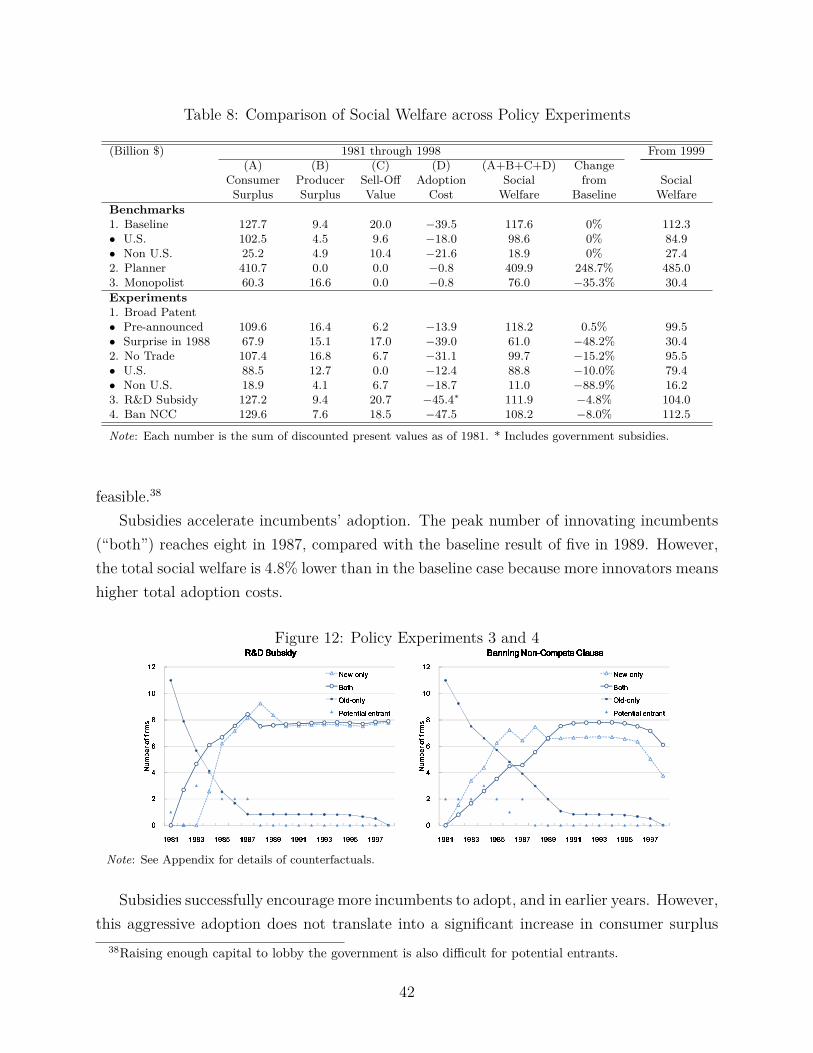
Table 8: Comparison of Social Welfare across Policy Experiments

(Billion $) 1981 through 1998 From 1999(A) (B) (C) (D) (A+B+C+D) Change

Consumer Producer Sell-Off Adoption Social from SocialSurplus Surplus Value Cost Welfare Baseline Welfare

Benchmarks1. Baseline 127.7 9.4 20.0 −39.5 117.6 0% 112.3• U.S. 102.5 4.5 9.6 −18.0 98.6 0% 84.9• Non U.S. 25.2 4.9 10.4 −21.6 18.9 0% 27.42. Planner 410.7 0.0 0.0 −0.8 409.9 248.7% 485.03. Monopolist 60.3 16.6 0.0 −0.8 76.0 −35.3% 30.4Experiments1. Broad Patent• Pre-announced 109.6 16.4 6.2 −13.9 118.2 0.5% 99.5• Surprise in 1988 67.9 15.1 17.0 −39.0 61.0 −48.2% 30.42. No Trade 107.4 16.8 6.7 −31.1 99.7 −15.2% 95.5• U.S. 88.5 12.7 0.0 −12.4 88.8 −10.0% 79.4• Non U.S. 18.9 4.1 6.7 −18.7 11.0 −88.9% 16.23. R&D Subsidy 127.2 9.4 20.7 −45.4∗ 111.9 −4.8% 104.04. Ban NCC 129.6 7.6 18.5 −47.5 108.2 −8.0% 112.5

Note: Each number is the sum of discounted present values as of 1981. * Includes government subsidies.

feasible.38

Subsidies accelerate incumbents’ adoption. The peak number of innovating incumbents(“both”) reaches eight in 1987, compared with the baseline result of five in 1989. However,the total social welfare is 4.8% lower than in the baseline case because more innovators meanshigher total adoption costs.

Figure 12: Policy Experiments 3 and 4

�

�

�

�

�

� �

� �

� � � ��

� ��

� � ��

! " # $ % & ' () % * +, ' - $ % & ' (. % * " & * / 0 ' " & * 1 0 & *

�

�

�

�

�

� �

� �

� � � �2� � � ��

� ��

3 4 5 5 � 5 6 7 8 53 4 5 5 � 5 6 7 8 53 4 5 5 � 5 6 7 8 53 4 5 5 � 5 6 7 8 5 99 99 : 8 ;=< > ? > : @ 4 � � >: 8 ;=< > ? > : @ 4 � � >: 8 ;=< > ? > : @ 4 � � >: 8 ;=< > ? > : @ 4 � � >

! " # $ % & ' () % * +, ' - $ % & ' (. % * " & * / 0 ' " & * 1 0 & *

Note: See Appendix for details of counterfactuals.

Subsidies successfully encourage more incumbents to adopt, and in earlier years. However,this aggressive adoption does not translate into a significant increase in consumer surplus

38Raising enough capital to lobby the government is also difficult for potential entrants.

42

for two reasons. First, a higher number of exits offsets a higher number of adopters. Second,potential entrants are less likely to enter due to preemption, and even if they do, they aremore likely to exit.

This result echoes some of the findings in the existing research. The effect of R&D subsidyhas been an active area of innovation studies, where a crucial policy question is whether R&Dsubsidies increase or decrease innovative activities in general, and private R&D spending inparticular.39 My experiment suggests R&D subsidy would increase the number of adopters,but public R&D spending would substitute for private R&D spending without inducing acomplementary increase in private R&D spending, because of the once-and-for-all nature ofinnovation in the technological context of the HDD industry. Although the nature of R&Defforts varies by industry, this experiment suggests a potential explanation for why studiestend to find small effects of public R&D spending in inducing private R&D.

Banning Non-compete Clauses (Experiment 4)As Scherer (1980) and Bresnahan (2003) emphasized as the (then) chief economists of the

Federal Trade Commission, entrants are important sources of innovation.40 Therefore, entryfacilitation is a potential channel through which public policy may promote innovation. Onepossible policy instrument concerns the legality of the private contracts governing the easeof starting new businesses. Specifically, the non-compete clause (NCC, or the covenants notto compete [CNC]) is the type of employment contract that limits the actions of personnelworking at an existing firm and considering starting their own businesses (or working for rivalfirms). Many HDD makers are headquartered in the American state of California, whereNCCs are banned. Nevertheless, exceptions to this ban exist, such as the cases involvingmergers, and the practice was common during the sample period.41 Of the 14 potentialentrants in my data, five Californian firms are founded by former managers and engineersfrom existing HDD makers, a typical Silicon Valley phenomenon. Thus a strict ban on NCCmay have important welfare implications through innovation and competition.

In this counterfactual, the five potential entrants founded by industry veterans appeartwo years earlier than in the actual data.

The two-year front-loading of the five entrants results in their earlier adoption. This front-loading does not materially alter the trajectory of incumbents. Social welfare decreases by8% because of increased adoption costs.

As in the case of more aggressive adoption by incumbents (section 7.2), earlier adoption39See Klette et al.’s (2000) survey.40Managers seem to agree, too. See Grove (1996) for the former Intel CEO’s account.41For instance, Finis Conner had to wait for two years before leaving Seagate Technology to found Conner

Technology in the late 1990s, because he had been a party to the merger between Seagate Technology andConner Peripheral in years prior to his departure.

43

tends to generate limited extra consumer surplus while raising the adoption costs substan-tially. Consumer surplus does not increase substantially, because the market size (the numberof potential buyers) is still small during the early years. Adoption costs increase becausethey are both initially high and discounted less.

44

References

[1] Acemoglu, Daron, and Dan Cao. 2010. “Innovation by Entrants and Incumbents.”Manuscript, MIT.

[2] Adner, Ron, and Peter Zemsky. 2005. “Disruptive Technologies and the Emergence ofCompetition.” RAND Journal of Economics, 36(2): 229-254.

[3] Arrow, Kenneth J. 1962. “Economic Welfare and the Allocation of Resources to In-vention.” In R.R. Nelson (Ed.), The Rate and Direction of Economic Activity. N.Y.,Princeton University Press.

[4] Benkard, C. Lanier. 2004. “A Dynamic Analysis of the Market for Wide-Bodied Com-mercial Aircraft.” Review of Economic Studies, 71: 581–611.

[5] Berry, Steven T.. 1994. “Estimating Discrete-Choice Models of Product Differentiation.”RAND Journal of Economics, 25(2): 242-262.

[6] ———, James Levinsohn, and Ariel Pakes. 1995. “Automobile Prices in Market Equi-librium.” Econometrica, 841–90.

[7] Bresnahan, Timothy F. 1981. “Departures from Marginal-Cost Pricing in the AmericanAutomobile Industry.” Journal of Econometrics, 17: 201–27.

[8] ———. 2003. “Pro-Innovation Competition Policy: Microsoft and Beyond.” CPRC Dis-cussion Paper, Competition Policy Research Center, Fair Trade Commission of Japan.

[9] Chesbrough, H. 1999. “Arrested development: The experience of European hard diskdrive firms in comparison to U.S. and Japanese firms.” Journal of Evolutional Eco-nomics, 9: 287–330.

[10] Christensen, Clayton M.. 1993. “The Rigid Disk Drive Industry: A History of Commer-cial and Technological Turbulence.” Business History Review, 67: 531-588.

[11] ———. 1997. The Innovator’s Dilemma. New York, HarperBusiness.

[12] Cohen, W.M. 2010. “Fifty Years of Empirical Studies of Innovative Activity and Per-formance.” Chapter 4 of B. Hall and M. Rosenberg eds., Handbook of the Economics ofInnovation, Volume 1. Amsterdam: Elsevier.

[13] Collard-Wexler, Allan. 2011. “Mergers and Sunk Costs: An application to the ready-mixconcrete industry.” Econometrica, forthcoming.

45

[14] Ericson, Richard, and Ariel Pakes. 1995. “Markov-Perfect Industry Dynamics: A Frame-work for Empirical Work.” Review of Economic Studies, 62: 53-82.

[15] Franco, April Mitchell, and Darren Filson. 2006. “Spin-Outs: Knowledge Diffusionthrough Employee Mobility.” RAND Journal of Economics, 37(4): 841–60.

[16] Fudenberg, Drew, and Jean Tirole. 1986. Dynamic Models of Oligopoly. London, Rout-ledge.

[17] Gilbert, Richard. 2006. “Looking for Mr. Schumpeter: Where Are We in theCompetition-Innovation Debate?” NBER.

[18] ———, and David Newbery. 1982. “Preemptive Patenting and the Persistence ofMonopoly.” American Economic Review, 72(2): 514-526.

[19] Goettler, Ronald, and Brett Gordon. 2011. “Does AMD spur Intel to innovate more?”Journal of Political Economy, 119(6): 1141-1200.

[20] Grove, Andrew S.. 1996. Only the Paranoid Survive: How to Exploit the Crisis Pointsthat Challenge Every Company and Career. New York, Currency Doubleday.

[21] Hausman, Jerry. 1996. “Valuation of New Goods under Perfect and Imperfect Compe-tition.” In T. Bresnahan and R. Gordon, eds., The Economics of New Goods, Studies inIncome and Wealth, Vol. 58, Chicago: National Bureau of Economic Research.

[22] Henderson, Rebecca M. 1993. “Underinvestment and Incompetence as Responses toRadical Innovation: Evidence from the Photolithographic Alignment Industry.” RANDJournal of Economics, 24(2): 248-270.

[23] ———, and Kim B. Clark. 1990. “Architectural Innovation: The Reconfiguration ofExisting Product Technologies and the Failure of Established Firms.” AdministrativeScience Quarterly, 35: 9–30.

[24] Hopenhayn, Hugo A.. 1992. “Exit, Selection, and the Value of Firms.” Journal of Eco-nomic Dynamics and Control, 16(3-4): 621-653.

[25] Igami, Mitsuru. 2013. “Offshoring as Process Innovation.” Manuscript, Yale University.

[26] Jaffe, Adam B., and Josh Lerner. 2004. Innovation and Its Discontents: How OurBroken Patent System Is Endangering Innovation and Progress, and What to Do aboutIt. Princeton, NJ: Princeton University Press.

46

[27] Jovanovic, Boyan. 1982. “Selection and the Evolution of Industry.” Econometrica, 50(3):649-670.

[28] King, A.A., and C.L. Tucci. 2002. “Incumbent entry into new market niches: The role ofexperience and managerial choice in the creation of dynamic capabilities.” ManagementScience, 48: 171–86.

[29] Klepper, Steven. 1996. “Entry, Exit, Growth, and Innovation over the Product LifeCycle.” American Economic Review, 86(3): 562-583.

[30] ———, and Peter Thompson. 2006. “Submarkets and the Evolution of Market Struc-ture.” RAND Journal of Economics, 37(4): 861-886.

[31] Klette, Tor Jakob, and Samuel Kortum. 2004. “Innovating firms and aggregate innova-tion.” Journal of Political Economy, 112(5): 986–1018.

[32] Klette, Tor J., Jarle Moen and Zvi Griliches. 2000. “Do Subsidies to Commercial R&DReduce Market Failure? Microeconometric Evaluation Studies.” Research Policy, 29(4–5): 471–495.

[33] Lerner, Joshua. 1994. “The Importance of Patent Scope: An Empirical Analysis.” RANDJournal of Economics, 25: 319–333.

[34] Lerner, Josh. 1997. “An Empirical Exploration of a Technology Race.” RAND Journalof Economics, 28(2): 228-247.

[35] McKendrick, David G., Richard F. Doner, and Stephan Haggard. 2000. From SiliconValley to Singapore: Location and Competitive Advantage in the Hard Disk Drive In-dustry. Stanford, CA: Stanford University Press.

[36] Nelson, Richard R., and Sidney G. Winter. 1978. “Forces generating and limiting con-centration under Schumpeterian competition.” Bell Journal of Economics, 9: 524–48.

[37] ———. 1982. “The Schumpeterian tradeoff revisited.” American Economic Review, 72:114–32.

[38] Nevo, Aviv. 2001. “Measuring Market Power in the Ready-to-eat Cereal Industry.”Econometrica, 69(2): 307–42.

[39] Pesendorfer, Martin. 2010. “Estimation of (Dynamic) Games: A Discussion.”Manuscript prepared for the World Congress (Econometric Society Monographs) onAdvances in Economics and Econometrics: Theory and Applications.

47

[40] Reinganum, Jennifer F.. 1983. “Uncertain Innovation and the Persistence of Monopoly.”American Economic Review, 73(4): 741–748.

[41] Rust, John. 1987. “Optimal Replacement of GMC Bus Engines: An Empirical Modelof Harold Zurcher.” Econometrica, 55(5): 999-1033.

[42] Ryan, Stephen P.. 2012. “The Costs of Environmental Regulation in a ConcentratedIndustry.” Econometrica, 80(3): 1019–61.

[43] Sah, R.J. and J.E. Stiglitz. 1986. “The architecture of economic systems: Hierarchiesand polyarchies.” American Economic Review, 76: 716–27.

[44] Sakakibara, Mariko and Lee Branstetter. 2001. “Do Stronger Patents Induce More In-novation? Evidence from the 1988 Japanese Patent Law Reforms.” RAND Journal ofEconomics, 32: 77–100.

[45] Scherer, F.M.. 1980. Industrial market structure and economic performance. Rand Mac-Nally, Chicago, IL.

[46] ——— and D. Ross. 1990. Industrial Market Structure and Economic Performance.Houghton Mifflin, Boston, MA.

[47] Schmidt-Dengler, Philipp. 2006. “The Timing of New Technology Adoption: The Caseof MRI.” Manuscript, London School of Economics.

[48] Schumpeter, Joseph A. 1934. The Theory of Economic Development. Cambridge, MA:Harvard University Press.

[49] ———. 1942. Capitalism, Socialism and Democracy. New York: Harper.

[50] Seim, Katja. 2006. “An Empirical Model of Firm Entry with Endogenous Product-TypeChoices.” RAND Journal of Economics, 37(3), 619-640.

[51] Stoneman, Paul, and Giuliana Battisti. 2010. “The Diffusion of New Technology.” Chap-ter 17 of B. Hall and M. Rosenberg eds., Handbook of the Economics of Innovation,Volume 1, Amsterdam: Elsevier.

[52] Su, Che-Lin. 2012. “Estimating Discrete-Choice Games of Incomplete Information: ASimple Static Example.” Manuscript, Chicago Booth.

[53] Sutton, John. 1998. Technology and market structure. MIT Press, Cambridge, MA.

48

[54] Sweeting, Andrew. 2012. “Dynamic Product Positioning in Differentiated Product Mar-kets: The Effect of Fees for Musical Performance Rights on the Commercial RadioIndustry.” Manuscript, Duke University.

[55] Tushman, Michael L., and Philip Anderson. 1986. “Technological Discontinuities andOrganizational Environments.” Administrative Science Quarterly, 31(3): 439-465.

[56] Weintraub, Gabriel Y., C. Lanier Benkard, Przemyslaw Jeziorski, and Benjamin VanRoy. 2008. “Nonstationary Oblivious Equilibrium.” Manuscript, Columbia University.

49

estimating the innovator’s dilemma: structural analysis...

Documents