estimating the magnitude and frequency of floods for

Estimating the Magnitude and Frequency of Floods for Streams in West-Central Florida, 2001

By K.M. Hammett and M.J. DelCharco

Scientific Investigations Report 2005-5080

U.S. Department of the Interior U.S. Geological Survey

ii

U.S. Department of the InteriorGale A. Norton, Secretary

U.S. Geological SurveyP. Patrick Leahy, Acting Director

U.S. Geological Survey, Reston, Virginia: 2005For sale by U.S. Geological Survey, Information Services Box 25286, Denver Federal Center Denver, CO 80225

For more information about the USGS and its products: Telephone: 1-888-ASK-USGS World Wide Web: http://www.usgs.gov/

Any use of trade, product, or firm names in this publication is for descriptive purposes only and does not imply endorsement by the U.S. Government.

Although this report is in the public domain, permission must be secured from the individual copyright owners to reproduce any copyrighted materials contained within this report.

Suggested Citation:

Hammett, K.M., and DelCharco, M.J., 2005, Estimating the Magnitude and Frequency of Floods for Streams in West-Central Florida, 2001: U.S. Geological Survey Scientific Investigations Report 2005-5080, 15 p., plus apps.

iii

CONTENTS

Abstract. . . . . . . . . . . . . . . . . . . . . . . . . . . . . . . . . . . . . . . . . . . . . . . . . . . . . . . . . . . . . . . . . . . . . . . . . . . . . . . . . . . . . . . . . . . . . . . . . . . . . 1Introduction . . . . . . . . . . . . . . . . . . . . . . . . . . . . . . . . . . . . . . . . . . . . . . . . . . . . . . . . . . . . . . . . . . . . . . . . . . . . . . . . . . . . . . . . . . . . . . . . . 1

Purpose and Scope . . . . . . . . . . . . . . . . . . . . . . . . . . . . . . . . . . . . . . . . . . . . . . . . . . . . . . . . . . . . . . . . . . . . . . . . . . . . . . . . . . . 2Previous Studies . . . . . . . . . . . . . . . . . . . . . . . . . . . . . . . . . . . . . . . . . . . . . . . . . . . . . . . . . . . . . . . . . . . . . . . . . . . . . . . . . . . . . . 2Description of the Study Area . . . . . . . . . . . . . . . . . . . . . . . . . . . . . . . . . . . . . . . . . . . . . . . . . . . . . . . . . . . . . . . . . . . . . . . . . 2

Data Used for Analyses. . . . . . . . . . . . . . . . . . . . . . . . . . . . . . . . . . . . . . . . . . . . . . . . . . . . . . . . . . . . . . . . . . . . . . . . . . . . . . . . . . . . . . 4Annual Peak Discharges. . . . . . . . . . . . . . . . . . . . . . . . . . . . . . . . . . . . . . . . . . . . . . . . . . . . . . . . . . . . . . . . . . . . . . . . . . . . . . 4Basin Characteristics . . . . . . . . . . . . . . . . . . . . . . . . . . . . . . . . . . . . . . . . . . . . . . . . . . . . . . . . . . . . . . . . . . . . . . . . . . . . . . . . . 4

Estimation of Flood Magnitude and Frequency at Gaged Sites . . . . . . . . . . . . . . . . . . . . . . . . . . . . . . . . . . . . . . . . . . . . . . . 4Log-Pearson Type III Frequency Analysis. . . . . . . . . . . . . . . . . . . . . . . . . . . . . . . . . . . . . . . . . . . . . . . . . . . . . . . . . . . . . . 5

Generalized Skew Coefficient and Weighted Skew . . . . . . . . . . . . . . . . . . . . . . . . . . . . . . . . . . . . . . . . . . . . . . 5Sensitivity to Long-Term Trends in Data . . . . . . . . . . . . . . . . . . . . . . . . . . . . . . . . . . . . . . . . . . . . . . . . . . . . . . . . . . 6Sensitivity to Historic Events Outside the Systematic Record . . . . . . . . . . . . . . . . . . . . . . . . . . . . . . . . . . . . . 7

Regression Analysis. . . . . . . . . . . . . . . . . . . . . . . . . . . . . . . . . . . . . . . . . . . . . . . . . . . . . . . . . . . . . . . . . . . . . . . . . . . . . . . . . . . 7Development of Multiple Regression Equations. . . . . . . . . . . . . . . . . . . . . . . . . . . . . . . . . . . . . . . . . . . . . . . . . . 7Regionalization of Regression Equations. . . . . . . . . . . . . . . . . . . . . . . . . . . . . . . . . . . . . . . . . . . . . . . . . . . . . . . . . 8Generalized Least Squares Regression Analysis . . . . . . . . . . . . . . . . . . . . . . . . . . . . . . . . . . . . . . . . . . . . . . . . . 8Sensitivity of Regression Equations . . . . . . . . . . . . . . . . . . . . . . . . . . . . . . . . . . . . . . . . . . . . . . . . . . . . . . . . . . . . . 10

Weighting of Log-Pearson Type III and Regression Analyses . . . . . . . . . . . . . . . . . . . . . . . . . . . . . . . . . . . . . . . . . 10Comparison with Previously Published Analyses . . . . . . . . . . . . . . . . . . . . . . . . . . . . . . . . . . . . . . . . . . . . . . . . . . . . . 11

Estimation of Flood Magnitude and Frequency at Ungaged Sites. . . . . . . . . . . . . . . . . . . . . . . . . . . . . . . . . . . . . . . . . . . . 13Sites With a Limited Period of Record or Without Discharge Data. . . . . . . . . . . . . . . . . . . . . . . . . . . . . . . . . . . . . 14Sites Upstream or Downstream from a Gaging Station . . . . . . . . . . . . . . . . . . . . . . . . . . . . . . . . . . . . . . . . . . . . . . . 14

Summary. . . . . . . . . . . . . . . . . . . . . . . . . . . . . . . . . . . . . . . . . . . . . . . . . . . . . . . . . . . . . . . . . . . . . . . . . . . . . . . . . . . . . . . . . . . . . . . . . . . 15Selected References. . . . . . . . . . . . . . . . . . . . . . . . . . . . . . . . . . . . . . . . . . . . . . . . . . . . . . . . . . . . . . . . . . . . . . . . . . . . . . . . . . . . . . . 15Appendix A. Basin characteristics and flood-discharge estimates for gaging stations, west-central

Florida . . . . . . . . . . . . . . . . . . . . . . . . . . . . . . . . . . . . . . . . . . . . . . . . . . . . . . . . . . . . . . . . . . . . . . . . . . . . . . . . . . A1-A8Appendix B. Annual peak discharge data for gaging stations, west-central Florida . . . . . . . . . . . . . . . . . .B1-B94

FIGURES

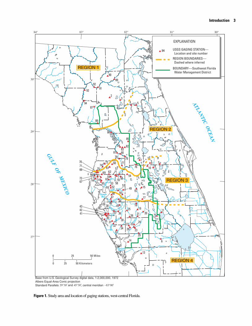
1. Map showing the study area and location of gaging stations, west-central Florida. . . . . . . . . . . . . . . . . .3

TABLES

1. Statistical summary of basin characteristics for gaging stations, west-central Florida. . . . . . . . . . . . . . .52. Significant trends in annual peak discharge data, west-central Florida. . . . . . . . . . . . . . . . . . . . . . . . . . . . . .63. Comparison of Bulletin 17B flood discharges computed from the continuous systematic record

and with inclusion of the 1912 historic flood at the Peace River at Arcadia, Florida. . . . . . . . . . . . . . . . . . .74. Regression equations for geographic regions, west-central Florida. . . . . . . . . . . . . . . . . . . . . . . . . . . . . . . . .95. Ranges of basin characteristics for geographic regions, west-central Florida. . . . . . . . . . . . . . . . . . . . . 10

iv

6. Sensitivity of the 25-year flood discharges to errors in basin characteristics. . . . . . . . . . . . . . . . . . . . . . . 117. Comparison of Bulletin 17B flood-discharge estimates from this study with Bulletin 17 or Bulletin

17A estimates from previous studies. . . . . . . . . . . . . . . . . . . . . . . . . . . . . . . . . . . . . . . . . . . . . . . . . . . . . . . . . . . . . . 128. Comparison of regression flood-discharge estimates from this study with regression estimates

from previous studies. . . . . . . . . . . . . . . . . . . . . . . . . . . . . . . . . . . . . . . . . . . . . . . . . . . . . . . . . . . . . . . . . . . . . . . . . . . . . 129. Comparison of weighted flood-discharge estimates from this study with weighted estimates

from previous studies. . . . . . . . . . . . . . . . . . . . . . . . . . . . . . . . . . . . . . . . . . . . . . . . . . . . . . . . . . . . . . . . . . . . . . . . . . . . . 13

Conversion Factors, Abbreviations, Acronyms, and Datum

Multiply By To obtain

foot (ft) 0.3048 meter

foot per mile (ft/mi) 0.1893 meter per kilometer

inch (in.) 2.54 centimeter

inch per year (in/yr) 2.54 centimeter per year

mile (mi) 1.609 kilometer

square mile (mi2) 2.590 square kilometer

cubic foot per second (ft3/s) 0.02832 cubic meter per second

cubic foot per second per year (ft3/s/yr) 0.02832 cubic meter per second per year

AEM average error of model

ASEP average standard error of prediction

DA drainage area

GIS geographic information system

LK percent of drainage area covered by lakes

SAMPE sampling error

SE standard error

SL slope

SWFWMD Southwest Florida Water Management District

USGS U.S. Geological Survey

Vertical coordinate information is referenced to the National Geodetic Vertical Datum of 1929 (NGVD 1929); horizontal coordinate information is referenced to the North American Datum of 1927 (NAD 27).

Estimating the Magnitude and Frequency of Floods for Streams in West-Central Florida, 2001

By K.M. Hammett and M.J. DelCharco

Abstract

Flood discharges were estimated for recurrence intervals of 2, 5, 10, 25, 50, 100, 200, and 500 years for 94 streamflow stations in west-central Florida. Most of the stations are located within the 10,000 square-mile, 16-county area that forms the Southwest Florida Water Management District. All stations had at least 10 years of homogeneous record, and none have flood discharges that are significantly affected by regulation or urbanization.

Guidelines established by the U.S. Water Resources Council in Bulletin 17B were used to estimate flood discharges from gag-ing station records. Multiple linear regression analysis was then used to mathematically relate estimates of flood discharge for selected recurrence intervals to explanatory basin characteris-tics. Contributing drainage area, channel slope, and the percent of total drainage area covered by lakes (percent lake area) were the basin characteristics that provided the best regression esti-mates. The study area was subdivided into four geographic regions to further refine the regression equations.

Region 1 at the northern end of the study area includes large rivers that are characteristic of the rolling karst terrain of northern Florida. Only a small part of Region 1 lies within the boundaries of the Southwest Florida Water Management Dis-trict. Contributing drainage area and percent lake area were the most statistically significant basin characteristics in Region 1; the prediction error of the regression equations varied with the recurrence interval and ranged from 57 to 69 percent.

In the three other regions of the study area, contributing drainage area, channel slope, and percent lake area were the most statistically significant basin characteristics, and are the three characteristics that can be used to best estimate the magnitude and frequency of floods on most streams within the Southwest Florida Water Management District. The Withlacoochee River Basin dominates Region 2; the prediction error of the regression models in the region ranged from 65 to 68 percent. The basins that drain into the northern part of Tampa Bay and the upper

reaches of the Peace River Basin are in Region 3, which had prediction errors ranging from 54 to 74 percent. Region 4, at the southern end of the study area, had prediction errors that ranged from 40 to 56 percent.

Estimates of flood discharge become more accurate as longer periods of record are used for analyses; results of this study should be used in lieu of results from earlier U.S. Geolog-ical Survey studies of flood magnitude and frequency in west-central Florida. A comparison of current results with earlier studies indicates that use of a longer period of record with addi-tional high-water events produces substantially higher flood-discharge estimates for many gaging stations. Another compar-ison indicates that the use of a computed, generalized skew in a previous study in 1979 tended to overestimate flood discharges.

Introduction

Population growth has resulted in rapid development throughout west-central Florida. The magnitude and frequency of flooding are important considerations in many design, plan-ning, and water management activities associated with develop-ment. Reliable estimates of flood-frequency characteristics are needed so that newly developed public and private infrastruc-tures are safeguarded and natural resources are protected.

The last systematic analysis of the flood-frequency characteristics of streams in west-central Florida included data through 1978. At that time (Bridges, 1982) about half of the continuous-record streamflow sites that were evaluated had less than 20 years of record. The length of a period of record can substantially affect the accuracy of flood-discharge estimates. Short periods of record are sensitive to sampling errors that result from chance geographical or temporal variations in rain-fall, and may be poor indicators of the long-term distribution of flood discharges at a site. By using longer periods of record, the accuracy of flood-discharge estimates in this report are improved compared with previous estimates.

2 Estimating the Magnitude and Frequency of Floods for Streams in West-Central Florida, 2001

Purpose and Scope

The purpose of this report is to: (1) present updated regional flood-frequency relations for streamflow gaging stations in west-central Florida for recurrence intervals of 2, 5, 10, 25, 50, 100, 200, and 500 years; and (2) present methods for estimating flood discharges at unregulated, rural sites where systematic data are not available or where the period of record is too short for individual analysis. Systematic data include annual peak discharge information observed by many Federal and state agencies, and by private enterprises (U.S. Water Resources Council, 1976).

More than 125 active and discontinued streamflow gaging stations in west-central Florida were evaluated for inclusion in the study. The methods included: compiling annual peak dis-charges and basin characteristics; fitting annual peak discharge data to a log-Pearson Type III frequency distribution using standard flood-frequency methods described in Bulletin 17B by the U.S. Water Resources Council (1982); examining annual peak discharge data for trends; developing multiple linear regression equations for distinct regions in the study area; and weighting station-specific flood-discharge data with regional regression estimates of flood discharge to determine flood frequency at gaged sites.

Previous Studies

Information presented in this report supersedes previous U.S. Geological Survey (USGS) estimates of the magnitude and frequency of flooding in west-central Florida. Earlier USGS studies that described flood-frequency characteristics in this area were prepared by Pride (1958), Barnes and Golden (1966), Rabon (1971), Seijo and others (1979), and Bridges (1982).

The first attempt to characterize and regionalize floods in Florida included data for 146 streamflow gaging stations with annual peak discharges determined by calendar year for data through 1953 (Pride, 1958). Flood-frequency distributions for each of the 146 stations were defined graphically. The State of Florida was subdivided into two homogeneous flood regions (A and B) on the basis of geometric similarities in the station flood-frequency graphs. All of west-central Florida was part of flood Region B. Composite frequency curves were then devel-oped for Regions A and B that defined ratios for determining up to the 50-year recurrence interval flood based on the mean annual flood at the station. Pride (1958) recognized that flood-water storage in lakes and marshes could substantially reduce flood magnitudes at some stations, and provided a method for adjusting flood magnitudes by accounting for attenuation that resulted from flood-water storage in the drainage areas upstream from selected stations.

All of Florida and parts of Mississippi, Alabama, and Georgia were included in the analyses prepared by Barnes and Golden (1966) as part of an evaluation of the magnitude and frequency of flooding throughout the United States. Annual peak discharges for each water year (October 1 through Sep-tember 30) were compiled for 549 streamflow gaging stations

in the southeastern United States (132 in Florida) with 5 or more years of record. The technique used by Barnes and Golden (1966) was similar to the one presented by Pride (1958) and is generally referred to as the index-flood method (Dalrymple, 1960). The South Atlantic Slope and Eastern Gulf of Mexico Basins evaluated by Barnes and Golden (1966) were subdivided into four homogeneous flood-frequency regions and 19 hydro-logic areas. West-central Florida was included in parts of two of the flood-frequency regions and further subdivided into three of the hydrologic areas defined by Barnes and Golden (1966). Floods with recurrence intervals of up to 50 years were esti-mated and a method was included for reducing flood discharges for those drainage basins where lakes and swamps provide flood-water storage.

Rabon (1971) was the first investigator to use multiple regression analysis as a way of regionalizing flood-frequency information for Florida. The main objective of his study was to determine the adequacy of the existing network to provide information at gaged sites and also to provide information that could be transferred to ungaged sites. Rabon (1971) evaluated the network for a wide range of discharge characteristics, including average and low discharges. Annual peak discharges for each of 145 gaging stations were mathematically fitted to a log-Pearson Type III distribution to determine the magnitude of floods with frequencies up to the 50-year recurrence interval. All of the stations had at least 10 years of record through 1970. Florida was subdivided into two homogeneous regions, with all of west-central Florida included in the ‘peninsular region.’

Seijo and others (1979) analyzed annual peak discharge data for 64 sites in west-central Florida using guidelines estab-lished by the U.S. Water Resources Council (1976) in Bulletin 17. A Pearson Type III distribution was fitted to logarithms of annual peak discharges from data through September 1976. West-central Florida was subdivided into three geographic regions and equations for each of the regions were developed using multiple regression analysis. The average standard error of estimate of the regional equations in Seijo and others (1979) was 43.5 percent.

Bridges (1982) analyzed annual peak discharge data for 182 sites throughout the State of Florida using the U.S. Water Resources Council (1977) Bulletin 17A guidelines and data through September 1978. Multiple regression analysis was used to develop equations for three geographic regions of the state. Because Bridges (1982) was evaluating data from the entire State, the geographic regions were different from those defined by Seijo and others (1979), particularly in the area of west-cen-tral Florida just north of Tampa Bay. The average standard error of estimate for the regional equations developed by Bridges (1982) was 56 percent.

Description of the Study AreaThe area of interest for this investigation includes about

10,000 mi2 of west-central Florida that drains to the Gulf of Mexico (fig. 1) and primarily is within the jurisdiction of the Southwest Florida Water Management District (SWFWMD).

Introduction 3Introduction 3

28°

27°

29°

30°

83°84° 82°

0 25 50 Miles

0 25 50 Kilometers

GU

LFO

FM

EX

ICO

and −83°00′

Base from U.S. Geological Survey digital data, 1:2,000,000, 1972Albers Equal-Area Conic projectionStandard Parallels , central meridian29°30′ 45°30′

REGION 1

WithlacoocheeR

iver

River

L

i t tle

Hill

sb

orough

Manat ee Rive

r

68

TampaBay

CharlotteHarbor

Mya

kka

River

Manatee Ri ver

Alafia River

23

87

89

90

9192

93

94

85

86

88

1

25

2728

303132

3334

35

36

39

4243

4445

40

46

4748 50

51452

5355 56

57

58

59

6162

63

66

67

69

7071

72

7475

78 79

8081

8283

84

6465

38

41 37

6073 77

5

Figure 1. Study area and location of gaging stations, west-central F

81° 80°

ATLANTIC

OC

EA

N

USGS GAGING STATION⎯ Location and site number

EXPLANATION

REGION BOUNDARIES−−Dashed where inferred

BOUNDARY−−Southwest FloridaWater Management District

94

REGION 3

REGION 2

REGION 4

Riv

er

Pea ce

4 5

13

4

1516

1819

21

22

23

24

26

29

9

6

11

17

2012

78

91076

1

4

lorida.


The Withlacoochee, Hillsborough, and Peace Rivers are the three largest river systems in the area. With a combined drain-age area of 5,100 mi2, the watersheds for the three rivers encompass more than half of the study area. Several smaller river basins are in the southern part of the study area. The Ala-fia, Manatee, and Little Manatee Rivers discharge into Tampa Bay and the Myakka River empties into Charlotte Harbor. In the area north of Tampa Bay, the Homosassa, Chassahowitzka, Weeki Wachee, and Crystal Rivers originate from coastal springs that discharge directly into tidally affected waters. The discharge of these rivers is not the result of runoff from surface drainage areas; instead they reflect the interaction of ground-water levels and tide stages. For these reasons, the coastal rivers north of Tampa Bay were not included in the flood-frequency analyses.

Land-surface elevations in the study area range from more than 200 ft above sea level in the headwaters of the Peace River to sea level along the coast of the Gulf of Mexico. Wetlands in the upper Hillsborough and Withlacoochee River Basins act as retention areas for flood waters, thereby attenuating the magni-tude of flood discharges. The upper reaches of the Peace River include many wetlands, and the area has been extensively strip-mined for phosphate ore, which has affected surface-runoff characteristics. The smaller southern basins extend through the coastal lowlands, and along some reaches, the flood plains are more than 2 mi wide. Small urban streams that receive most of their runoff from impervious roadways and parking lots can rise rapidly after intense rainfall; but because of low topo-graphic relief and the storage capacity in stormwater ponds, lakes, swamps, and marshes, it generally takes several days for larger river systems in west-central Florida to crest during flood events. Streams that have discharges significantly affected by urbanization were not included in this study.

The climate of the area is subtropical and humid. Rainfall averages about 52 in/yr, with more than half occurring during the summer months from June to September. Major floods are most likely to result from rainfall associated with tropical depressions, tropical storms, or hurricanes and are most likely to occur in Sep-tember or October, near the end of the summer rainy season. Intense convective thunderstorms, however, have produced more than 15 in. of rain in 24 hours and caused substantial local-ized flooding in early summer; broad winter frontal systems sometimes cause high-water events in February or March.

Data Used for AnalysesAnnual peak discharges (gaged sites) and basin character-

istics (gaged or ungaged sites) are the two types of information needed to estimate flood frequencies. The analysis of historical annual peak discharge data allows for accurate estimates of flood frequency and magnitude at sites where there are stream-flow gaging stations. To estimate flood discharges at a gaged site, the annual peak discharges for the period of record are fitted to a log-Pearson Type III frequency distribution, using criteria established by the U.S. Water Resources Council (1982) in Bulletin 17B.

To estimate flood discharges at sites that have limited or no historical data, flood-discharge estimates from gaging stations are transferred to locations without gaged record using statistical regression. Estimates of flood discharges at gaged sites are mathematically related to basin characteristics such as drainage area and basin slope using multiple linear regression methods. Regression equations are then used to estimate the flood discharges at ungaged sites using the basin characteristics of those ungaged sites as input values in the equations.

Annual Peak Discharges

Annual peak discharge is the highest instantaneous dis-charge recorded at a site for an independent flood event during the water year. Occasionally, the annual peak may not be the maximum discharge for the year. In such cases, the maximum discharge occurs at midnight at the beginning or end of the water year, on a recession from or rise toward a higher peak in an adjoining year. Annual peak discharge data through the 2001 water year were used for this investigation. Data for 94 USGS streamflow gaging stations in west-central Florida were included; 75 of the stations are within the boundaries of the SWFWMD and 19 are along the periphery. All of the stations had at least 10 years of homogeneous record. Streamflow gaging stations that have flood discharges significantly affected by regulation or urbanization were not included. All of the sites evaluated in this report are shown in figure 1, and listed in appendix A. Annual peak discharge data are presented in appendix B.

Basin Characteristics

Basin characteristics were compiled from previously published reports, the USGS basin characteristics database, and geographic information system (GIS) databases. Only three characteristics—contributing drainage area, channel slope, and the percent of the total drainage area covered by lakes—were found to be statistically significant in describing the variability of flood discharges at gaging stations, and only those three are presented in this report. Basin characteristics for the 94 stations used for this study are statistically summarized in table 1 and listed for individual stations in appendix A.

Estimation of Flood Magnitude and Frequency of Gaged Sites

Flood-frequency analysis is the procedure in which annual peak discharge data are fitted to a theoretical frequency distri-bution. The U.S. Water Resources Council (1982) in Bulletin 17B has recommended use of the log-Pearson Type III distribu-tion as the standard for defining the flood-frequency distribu-tion at gaging stations.

Estimation of Flood Magnitude and Frequency of Gaged Sites 5

Table 1. Statistical summary of basin characteristics for gaging stations, west-central Florida.

[mi2, square mile; ft/mi, feet per mile]

StatisticSample

(number ofpeaks)

Drainage area(mi2)

Slope1

(ft/mi)Lake area2

(percent)

Mean 33.9 407.5 3.27 3.70

Median 28 77.3 2.63 1.80

Maximum 72 9,640 23.5 27.5

Minimum 11 0.94 0.09 0

Standard deviation 18.3 1,407 2.86 5.201Channel slope between points 10 and 85 percent of the distance from the station to the ba-

sin boundary.2Percentage of drainage area covered by lakes.

Log-Pearson Type III Frequency Analysis

The log-Pearson Type III distribution is defined by the equation:

log QT = M + kS

where

The USGS developed PEAKFQ software to fit the log-Pearson Type III distribution to annual peak discharge data and to compute flood-frequency estimates at streamflow stations based on Bulletin 17B guidelines. The software is nonpropri-etary and can be accessed and downloaded from the USGS web site: (http://water.usgs.gov/usgs/software/Surface_Water/ watstore.html) for use on UNIX or DOS operating systems. Bulletin 17B flood-frequency estimates for all of the stations used in this study were computed using PEAKFQ and are included in appendix A.

Generalized Skew Coefficient and Weighted Skew

The skew coefficient is a measure of the asymmetry of the distribution of annual peak discharge data, and is sensitive to extreme events. A single high event during a short period of

QT is the flood discharge for a selected recurrence interval T, in cubic feet per second;

M is the mean of the logarithms of the annual peak discharges;

k is the Pearson Type III frequency factor, which is a function of the skew coefficient of the logarithms of the annual peak discharges and the recurrence interval, (tables of k values are provided in Bulletin 17B); and

S is the standard deviation of the logarithms of the annual peak discharges.

record can result in an inaccurate estimate of the asymmetry of the flood-frequency distribution for an individual station. The skew coefficient tends to have greater variability between sam-ples than the mean and standard deviation. Consequently, it is considered a less reliable estimator of a population statistic for a particular site. Several procedures have been proposed to improve the reliability of the sample skew coefficient in estimat-ing the population skew. Bulletin 17B recommends weighting the skew coefficient computed for an individual station with a gener-alized skew coefficient that represents the average skew for nearby stations. The weighted skew combines the station and generalized skews by weighting them in inverse proportion to their individual mean-square errors. The weighting procedure recommended in Bulletin 17B is different than the procedure presented in Bulletin 17 or Bulletin 17A and tends to reduce the influence of the generalized skew and increase the influence of the station skew.

Bulletin 17B presents methods for determining a general-ized skew. One method is to use the generalized skew map of the United States that was prepared as part of the original release of Bulletin 17 (U.S. Water Resources Council, 1976) and was based on data through 1973. The national map shows that the generalized skew for west-central Florida ranges between 0.0 and -0.1. As an alternate method, the generalized skew can be computed as the average of the station skews for stations that have 25 or more years of record. This alternate pro-cedure requires at least 40 long-term stations or all long-term stations within a 100-mi radius of the area of interest.

Seijo and others (1979) computed a generalized skew coefficient of 0.14 for west-central Florida using the average of the station skew coefficients for a group of 29 stations having over 25 years of record. The range of skew coefficients for the 29 stations was -0.81 to 1.02. Seijo and others (1979) used the computed generalized skew because it was substantially differ-ent than the map values in Bulletin 17 (U.S. Water Resources Council, 1976).


For this study, there were 57 stations with periods of record 25 years or longer. The computed average of the skew coefficients for those 57 stations was -0.16, the range was -2.21 to 0.89, and the standard deviation was 0.57. Because the com-puted average skew was not substantially different from the Bulletin 17 map skews, the map values were used for general-ized skews in the computations.

The additional years of annual peak discharge data that have been recorded since Seijo and others (1979) completed their analyses have had a substantial effect on computed skew coefficients. If the additional years of data are included for the 29 stations originally used by Seijo and others (1979), then the computed average skew coefficient changes from 0.14 to 0.03. The availability of 28 more long-term stations has also affected the computation, reflecting a greater negative generalized skew (-0.16). Thus, the map values from Bulletin 17 can be used with greater confidence for the area of west-central Florida.

As recommended in Bulletin 17B, PEAKFQ software allows the user to weight the station skew coefficient with the generalized skew coefficient to compute the log-Pearson Type III flood-frequency distribution for a station. The station skew and generalized skew are weighted inversely to their respective mean-square errors. Because the mean-square error of the sta-tion skew increases as the length of record decreases, weighted skew coefficients for stations with short periods of record can be significantly adjusted by generalized skews. For stations with long periods of record, the station skew has the greater importance in the computation of a weighted skew coefficient. The Bulletin 17B flood discharges presented in appendix A represent computations based on weighted skew coefficients.

Sensitivity to Long-Term Trends in Data

Trends in annual mean discharge data for several streams in west-central Florida have been documented in previous investigations (Hammett, 1990; Stoker and others, 1996).

Table 2. Significant trends in annual peak discharge data, wes

[ft3/s, cubic feet per second]

Stationnumber

Site nameP

sy

02270500 Arbuckle Creek near De Soto City 19

02295637 Peace River at Zolfo Springs 19

02296750 Peace River at Arcadia 19

02301500 Alafia River at Lithia 19

02310000 Anclote River near Elfers 19

02310800 Withlacoochee River near Eva 19

02312640 Jumper Creek Canal near Bushnell 19

The nonparametric Kendall Tau test (Helsel and Hirsch, 1992) was used to determine whether there were trends in the system-atic annual peak discharge data for stations included in this study.

Seven of these stations did have trends in annual peak discharges where the statistical level of significance was 0.02 or less. These stations are listed in table 2 along with the period of continuous record, the slope of the trend, and the statistical level of significance. The slope corresponds to the change per year in annual peak discharge over the period of record. For example, the trend in the Peace River at Zolfo Springs has a slope of -49.18 ft3/s/yr. The annual peak discharge at the Peace River at Zolfo Springs averaged 5,370 ft3/s for the 69 years of record, so a decrease of 49.18 ft3/s/yr is less than 1 percent of the aver-age annual peak per year; however, a cumulative decrease of 3,295 ft3/s (49.18 ft3/s/yr *67 years) from 1934 to 2001 is substantial.

Climatic variability has had some impact on the decreasing trends shown in table 2. Within the study area, tropical cyclones were both more numerous and more intense during the 30 years before 1960 than during the 30 years after 1960. There are, how-ever, several stations in the study area with equally long periods of record that were affected by the same weather patterns but do not have statistically significant declines in their annual peak discharges.

Hammett (1990) reported that decreasing trends in the annual mean discharges of sites in the Peace River Basin were probably related to a long-term decline in the potentiometric surface of the underlying aquifer and a resulting reduction of ground-water inflow to the river. The decreasing trends in annual peak discharges at the Peace River stations at Zolfo Springs and Arcadia may also reflect some impact of reduced ground-water inflow. Because annual mean discharges have declined over the period of record, there is more area available for storing flood waters in the basin when heavy rainfall occurs. Consequently, the peak discharges may be lower partly because of lower antecedent water-level conditions.

t-central Florida.

eriod of stematicrecord

Kendall’sTau

Significancelevel

Median slope(ft3/s

per year)

Average ofannual peak

discharges(ft3/s)

40-2001 -0.21 0.015 -15.64 1,989

33-2001 -0.29 0.001 -49.18 5,370

31-2001 -0.27 0.001 -60.67 8,513

33-2001 -0.21 0.012 -27.73 4,358

45-2001 -0.22 0.017 -11.09 1,080

59-1993 -0.33 0.006 -12.06 376

64-2001 -0.44 0.000 - 2.48 84


Table 3. Comparison of Bulletin 17B flood discharges computed from the continuous systematic record and with inclusion of the 1912 historic flood at the Peace River at Arcadia, Florida.

[Discharge in cubic feet per second]

Recurrenceinterval(year)

Flood discharge from continuous data

1931-2001

Flood discharge, including 1912 historic flood

2 6,220 6,270

5 10,900 11,300

10 14,900 15,800

25 21,200 23,200

50 26,900 30,000

100 33,400 38,200

200 41,000 47,900

500 53,000 63,600

Stoker and others (1996) documented a decreasing trend in the annual mean discharges of the Alafia River, and reported that it was most likely related to the long-term decline in the potentiometric surface of the underlying aquifer. Annual peak discharges on the Alafia River may have been impacted for the same reasons noted for the Peace River Basin.

The U.S. Water Resources Council (1993) Subcommittee on Hydrology evaluated possible methods for adjusting flood-frequency distributions to reflect either episodic changes or secular trends in watersheds. Channel straightening is an exam-ple of an episodic change and gradual urbanization is an exam-ple of a secular trend that could impact the flood-frequency characteristics of a watershed. The methods presented by the Subcommittee on Hydrology were recommended for use only where there was physical evidence of change in a substantial part of the watershed. There are, however, no guidelines for determining what constitutes a substantial part of the water-shed. Also, there are no easy methods for isolating the variation induced by a secular trend from the random variation resulting from climatic patterns.

The decreasing trends identified in table 2 cannot be defin-itively subdivided or proportioned by cause. Because there is no technically defensible basis on which to adjust the data for some amount of secular trend, the historic data were used for all further analyses in this study. The user should, however, be aware that flood-discharge estimates for the stations listed in table 2 have a substantial degree of uncertainty as a result of statistically significant trends in the annual peak series.

Sensitivity to Historic Events Outside the Systematic Record

Historic photographs and records of high-water marks can provide valuable extensions to continuous records at gag-ing stations. The U.S. Water Resources Council (1982) pro-vides a method for including such historic flood events that occurred before or after the period of continuous systematic data collection. In table 3, the Bulletin 17B flood discharges computed for the period of continuous data collection at the Peace River at Arcadia (site 22, fig. 1) are compared with flood discharges computed including the historic 1912 flood event, which had an estimated discharge of 43,000 ft3/s and produced the highest water level ever documented at the site.

Including the 1912 flood in the computation of flood discharges has a minor effect on discharge at lower recurrence intervals, but it raises the discharges associated with less fre-quent events. All historic events outside the period of continu-ous record that were well documented were used in the analyses for this study and are included in appendix B.

Regression Analysis

Regression analysis was used to mathematically relate basin characteristics to estimates of flood magnitude and fre-quency at gaging stations. Explanatory variables such as the

contributing drainage area, channel slope, percent lake area, and so on, were related to 2-, 5-, 10-, 25-, 50-, 100-, 200-, and 500-year flood discharges that had been calculated using Bulletin 17B criteria. Equations computed from the regression analyses can then be used to calculate flood-discharge estimates at sites where basin characteristics are known, but for which no dis-charge data are available.

Development of Multiple Regression Equations

The multiple regression equations used in this study have the general form:

QT = C X1B1 X2

B2 X3B3....Xn

Bn (1)

which can be expressed in the linear form:

LogQT = LogC + B1LogX1 + B2LogX2

+ B3LogX3 + ....... + BnLogXn (2)

where

Methods for developing good multiple linear regression equations, described in detail by Helsel and Hirsch (1992), were used for this study. Basin characteristics were checked for multi-collinearity (interdependence) and co-related charac-teristics were selected for elimination prior to performing any regression analyses. Preliminary multiple linear regression

QT is the flood discharge for the T-year recurrence interval;

C is the regression constant for the T-year recurrence interval;

X1 to Xn are the (explanatory variables) basin characteristics; and

B1 to Bn are the regression coefficients for the T-year recurrence interval.


analyses were performed using an all-regression procedure in the STATIT software package (Statware, Inc., 1990); all possible combinations of explanatory variables were evaluated to determine which basin characteristics were most significant. Preliminary regression models were evaluated for best fit based on the value of Mallow’s Cp (Helsel and Hirsch, 1992, p. 312). The models were further evaluated by examining the root mean square error, coefficient of determination (R2) and adjusted R2 for each model, and the significance level of the independent variables. Stations with statistically significant trends in annual peak discharge (table 2) were not included in development of regression equations.

Based on evaluation of all possible combinations of explanatory variables, contributing drainage area (DA), main channel slope (SL), and percent of the total drainage area cov-ered by lakes (LK), provided the best regression models for the study area. Contributing drainage area was the most significant variable, whereas slope and lake area varied in significance with the recurrence interval. Bridges (1982) and Seijo and others (1979) also found these variables to be significant in their regression analysis.

As in previous studies, common log transformations were used for all variables in the regressions. Because some values of percent lake area were zero, it was not possible to transform that characteristic without addition of a constant for all sites. The addition of a small constant is a standard procedure when attempting to use log transformations with some zero values (Haan, 1977, p. 146). Bridges (1982) added a constant of 3.0 or 0.6 to the lake area characteristic, depending on the region in which the site was located. Constants of 3.0 or 0.6 also were used for this study using the same geographic regions.

Regionalization of Regression Equations

The accuracy of regression equations can sometimes be improved by grouping stations geographically and defining equations for the subdivided regions. The ordinary least squares method was used to compute a regression equation for 25-year flood discharges, using data for the 87 stations without statistically significant trends. The regression residuals were then plotted on a map to determine if there were regional pat-terns that could be used to define geographic subsets. Potential subdivisions also were compared to geographic regions previ-ously delineated by Bridges (1982) and Seijo and others (1979). Once regions were identified, the nonparametric Wilcoxon signed-ranks test was used to test the significance of the differ-ences between the groups of residuals. Four regions were defined for subdivision for this study and are shown in figure 1.

Hydrologically similar rivers and streams are grouped by their geographic location. Region 1 includes large rivers, such as the Suwannee and Santa Fe, that are representative of the karst regions and rolling hills of northern Florida. Region 2 includes the Withlacoochee River Basin, which typically has more low-lying areas and wetlands than Region 1. Region 3 includes the Hillsborough, Alafia, and upper Peace River

Basins. The lower Peace River Basin and many of the smaller coastal streams draining west to the Gulf of Mexico are in Region 4. After the geographic subdivisions were defined, regression equations were developed for each of the regions.

Generalized Least Squares Regression Analysis

Tasker and Stedinger (1989) showed that model error from an ordinary least squares regression can be reduced by using a generalized least squares regression, which takes into consideration the time-sampling error of flood-discharge char-acteristics and the correlation of flood-discharge characteristics between nearby stations. In generalized least squares analysis, the total prediction error is partitioned into model error and sampling error, making it possible to identify errors due to inad-equacies of model formulation compared with deficiencies in the database. Generalized least squares regression has been incorporated into the USGS software program GLSNET, which is nonproprietary and can be accessed and downloaded for UNIX and DOS operating systems from the USGS web site: (http://water.usgs.gov/software/glsnet.html). GLSNET was used to compute the final regression equations for each geographic region (table 4).

GLSNET provides estimates for the model error and sam-pling error. The model error is a measure of the error in the model that cannot be changed by collecting more data and is presented as the average error of the model (AEM). The stan-dard error of the model in percent (SEm) is presented in table 4 and is calculated from AEM using the following equation:

SEm (%) = 100*[e (5.3019 * AEM**2) – 1] ½ (3)

where AEM is the average error of the model in base 10 log units.

The standard error of the model is asymmetrical and so it is useful to present both sides of the percent error using the following equations:

SEm (+%) = 100*[ (10 **AEM ) – 1] and (4)

SEm (-%) = 100*[ (10 **( –AEM) ) – 1] (5)

The sampling error (SAMPE) is the error in predicting flood discharges that is introduced by the generalized least squares regression method. The error introduced by the gener-alized least squares method typically is much lower than the error introduced by ordinary least squares methods and is the reason generalized least squares is preferred (Stedinger and Tasker, 1985). In table 4, the average standard error of predic-tion (ASEP), in percent, is a measure of how well the regression model predicts flood discharges, and can be computed using the following equation:


Table 4. Regression equations for geographic regions, west-central Florid

Regression equationsStandard errorof model, SEm

(percent)

Region

Q2 = 132 (DA)0.528 (LK+0.6) -0.542 57.9

Q5 = 267 (DA)0.510 (LK+0.6) -0.534 50.3

Q10 = 389 (DA)0.500 (LK+0.6) -0.535 48.3

Q25 = 583 (DA)0.489 (LK+0.6) -0.540 47.1

Q50 = 760 (DA)0.481 (LK+0.6) -0.545 46.9

Q100 = 965 (DA)0.474 (LK+0.6) -0.550 47.0

Q200 = 1,200 (DA)0.467 (LK+0.6) -0.557 47.4

Q500 = 1,562 (DA)0.460 (LK+ 0.6)-0.566 48.4

Region

Q2 = 2.03 (DA)1.065 (LK+3.0)-0.259 (SL)-0.017 57.3

Q5 = 5.82 (DA)1.023 (LK+3.0)-0.339 (SL)0.149 54.9

Q10 = 9.84 (DA)0.999 (LK+3.0)-0.371 (SL)0.226 54.7

Q25 = 17.0 (DA)0.972 (LK+3.0)-0.398 (SL)0.298 54.3

Q50 = 24.1 (DA)0.953 (LK+3.0)-0.412 (SL)0.339 54.0

Q100 = 32.7 (DA)0.936 (LK+3.0)-0.423 (SL)0.372 53.5

Q200 = 42.8 (DA)0.921 (LK+3.0)-0.432 (SL) 0.400 52.9

Q500 =58.7 (DA)0.903 (LK+3.0)-0.440 (SL) 0.428 52.3

Region

Q2 = 21.0 (DA)0.890 (LK+3.0)-0.601 (SL)0.452 54.6

Q5 = 54.0 (DA)0.841 (LK+3.0)-0.593(SL)0.374 49.1

Q10 = 87.2 (DA)0.819 (LK+3.0)-0.594 (SL)0.338 49.9

Q25 = 140 (DA)0.799 (LK+3.0)-0.593 (SL)0.308 52.6

Q50 = 186 (DA)0.789 (LK+3.0)-0.591 (SL)0.294 55.2

Q100 = 236 (DA)0.782 (LK+3.0)-0.588(SL)0.284 57.9

Q200 = 289 (DA)0.776 (LK+3.0)-0.584 (SL) 0.278 60.9

Q500 = 364 (DA)0.771 (LK+3.0)-0.578 (SL) 0.274 64.9

Region

Q2 = 62.3 (DA)0.661 (LK+3.0)-0.367 (SL)0.497 36.3

Q5 = 127 (DA)0.669 (LK+3.0)-0.435 (SL)0.493 35.9

Q10 = 182 (DA)0.678 (LK+3.0)-0.474 (SL)0.495 37.0

Q25 = 262 (DA)0.691 (LK+3.0)-0.514 (SL)0.502 38.9

Q50 = 326 (DA)0.701 (LK+3.0)-0.538 (SL)0.508 40.7

Q100 = 394 (DA)0.712 (LK+3.0)-0.559 (SL)0.513 42.6

Q200 = 465 (DA)0.722 (LK+3.0)-0.576 (SL) 0.519 44.7

Q500 = 562 (DA)0.736 (LK+3.0)-0.595 (SL) 0.527 47.6

a.

SEm(+ percent)

SEm(– percent)

Average standard error of prediction (ASEP)

(percent)

Equivalent length of record (years)

1

71.2 -41.6 69 1.35

60.8 -37.8 60 2.29

58.0 -36.7 58 3.27

56.5 -36.1 57 4.64

56.2 -36.0 58 5.64

56.4 -36.1 58 6.58

56.9 -36.3 59 7.43

58.2 -36.8 61 8.41

2

70.3 -41.3 68 1.98

67.1 -40.1 65 2.58

66.7 -40.0 65 3.34

66.3 -39.9 66 4.48

65.8 -39.7 66 5.39

65.2 -39.5 66 6.34

64.4 -39.2 66 7.31

63.5 -38.8 66 8.59

3

66.7 -40.0 60 1.99

59.1 -37.2 54 3.02

60.2 -37.6 56 3.85

63.9 -39.0 59 4.74

67.4 -40.3 62 5.27

71.3 -41.6 66 5.69

75.4 -43.0 69 6.02

80.9 -44.7 74 6.36

4

42.1 -29.6 40 3.86

41.7 -29.4 40 5.44

43.1 -30.1 42 6.91

45.6 -31.3 45 8.65

47.9 -32.4 47 9.74

50.5 -33.5 50 10.62

53.2 -34.7 52 11.33

57.1 -36.4 56 12.04


Table 5. Ranges of basin characteristics for geographic regions, west-central Florida.

Basin characteristic Region 1 Region 2 Region 3 Region 4

Drainage area (square miles) 18.5 – 9,640 28.6 – 2,100 4.43 – 390 0.94 – 330

Slope (feet per mile) 0.51 – 23.5 0.09 – 3.6 0.41 – 9.8 1.02 – 7.52

Lake area (percent) 0.03 – 8.67 0 – 26.35 0 – 27.5 0 – 19.3

ASEP = 100*[e (5.3019 *(AEM**2+SAMPE**2) – 1] ½ (6)

where AEM and SAMPE are in base 10 log units.

Another measure of the reliability of regression equations was described by Hardison (1971) and is expressed as the equivalent years of record (table 4) needed at a newly estab-lished gaging station to achieve results of equal accuracy. For example, if the regression equations are used to estimate the 100-year recurrence interval flood discharge for a site on a stream in Region 4, the estimate would be equivalent in accu-racy to an estimate of the 100-year flood discharge computed from 10.62 years (table 4) of field data. GLSNET provides a computation of equivalent years of record for each regression.

The errors presented in table 4 are applicable only when the equations are used for sites where the values of basin char-acteristics fall within the range of values used to develop the equations. Extrapolating the regression equations for applica-tion to watersheds that have characteristics outside the range would produce flood estimates with unpredictable errors. The ranges of basin characteristics for each geographic region are presented in table 5.

Sensitivity of Regression Equations

To evaluate how errors in measuring basin characteristics could affect estimates of flood discharge computed from the regression equations, a sensitivity analysis was performed. For each geographic region, the 25-year flood discharge was computed by using the regression equation and applying incre-mental changes in the individual basin characteristics. The “reference” 25-year flood discharge was computed using the mean values of the basin characteristics for that geographic region (table 6). Then, each basin characteristic was changed by decreasing and increasing the mean value by 10, 20, and 30 percent, whereas the values of the other basin characteristics were held constant.

Results of this analysis show that in geographic Region 1, both basin characteristics have about the same amount of influ-ence on the equation, but in opposite directions. For example, underestimating the drainage area by 10 percent would result in a 5 percent decrease in the computed 25-year flood discharge whereas underestimating lake area by 10 percent would result in a 5 percent increase in the computed 25-year flood discharge. For geographic Regions 2, 3, and 4, the equations are more sen-sitive to changes in drainage area than to changes in the other

basin characteristics. In Region 2, the regression coefficient for drainage area is nearly equal to 1.0, making the decrease or increase in 25-year flood discharge almost directly proportional to the decrease or increase in drainage area. In Region 3, errors in percent lake area would have the second greatest effect on flood discharge, and in Region 4, errors in basin slope would have the second biggest effect.

Weighting of Log-Pearson Type III and Regression Analyses

Regression equations can be used to compute estimates of flood discharges at locations where no historic records of dis-charge are available; they can also be used to improve estimates of flood discharges at stations where data are available. The U.S. Water Resources Council (1982) presents a method of weighting the values from Bulletin 17B (standard log-Pearson Type III estimates computed from station records) with the values computed from regression equations. This weighting is based on the period of record at the station and equivalent years record represented by the regression equation. The weighted flood-dis-charge estimates are considered the most accurate estimates and should be the values used to describe flood-frequency charac-teristics at gaging stations. The weighting equation is:

QTwtd = (Q17B*N + Qreg *EQ) / (N + EQ) (7)

where

Weighted flood-discharge estimates are presented in appendix A, along with the Bulletin 17B estimates and the regression estimates.

QTwtd is the weighted flood discharge for the T-year recurrence interval;

Q17B is the flood discharge for the T-year recurrence interval computed from the station record using Bulletin 17B guidelines;

Qreg is the flood discharge for the T-year recurrence interval computed from the regression equation;

N is the number of years of station data used to compute Q17B; and

EQ is the equivalent years of record for the regression equation from table 4.


Table 6. Sensitivity of the 25-year flood discharges to errors in basin characteristics.

Change in computed 25-year flood discharge (percent)

Basin characteristic Error in basin characteristic (percent)

-30 -20 -10 Reference +10 +20 +30

Region 1

Drainage area (DA) -16 -10 -5 0 5 9 14

Lake area (LK) 16 10 5 0 -4 -8 -11

Region 2

Drainage area (DA) -29 -19 -10 0 10 19 29

Lake area (LK) 10 6 3 0 -3 -5 -7

Slope (SL) -10 -6 -3 0 3 6 8

Region 3

Drainage area (DA) -25 -16 -8 0 8 16 23

Lake area (LK) 13 8 4 0 -3 -7 -9

Slope (SL) -10 -7 -3 0 3 6 8

Region 4

Drainage area (DA) -22 -14 -7 0 7 13 20

Lake area (LK) 6 4 2 0 -2 -3 -5

Slope (SL) -16 -11 -5 0 5 10 14

Comparison with Previously Published Analyses

Estimates of flood discharges for three stations used in this study are compared with estimates presented in Bridges (1982) and Seijo and others (1979) to illustrate the effects of changes in methodology, changes in regression equations, and changes in the length of record (tables 7, 8, and 9, respectively). The first station, Manatee River near Bradenton (site 37, fig. 1) was discontinued in 1966; all three studies used the same data for that station. The other two stations, Horse Creek near Arcadia (site 27, fig. 1) and Cypress Creek near San Antonio (site 61, fig. 1), have data sets with substantially longer periods of record than were used in Bridges (1982) or Seijo and others (1979).

The effect of changes in methodology used to analyze individual station records is compared in table 7 for estimates for the Manatee River near Bradenton (site 37, fig. 1). All three of the flood-frequency studies used the same data set for the station. This study used U.S. Water Resources Council (1982) Bulletin 17B criteria and Bridges (1982) used the U.S. Water Resources Council (1977) Bulletin 17A criteria. Seijo and others (1979) used the U.S. Water Resources Council (1976) Bulletin 17 guidelines and a computed generalized skew, rather than a map skew, weighted with the station skew. For floods with recurrence intervals of 50 years or less, there is less than a 1 percent difference between Bulletin 17B estimates for this

station and Bulletin 17A estimates computed by Bridges (1982). The maximum difference between the two methods is 3 percent, which occurs for the 500-year recurrence interval. The use of a computed generalized skew rather than the Bulletin 17 map skew by Seijo and others (1979) has a much greater effect on the estimates of flood discharge for the station. For the 25-year recurrence interval flood, the estimate by Seijo and others (1979) is about 5 percent higher than estimates computed using Bulletin 17B. For the 500-year recurrence interval flood, the estimate by Seijo and others (1979) is about 20 percent higher.

Estimates computed from the regression equations devel-oped in this study are compared with regression estimates from Bridges (1982) and Seijo and others (1979) in table 8. The dif-ferences in the regression estimates reflect changes in the geo-graphic grouping of the stations and differences in the explanatory variables used in the equations, as well as changes in methodology and longer periods of record (table 7). Bridges (1982) included all three stations in table 8 in one geographic region. This study and Seijo and others (1979) placed Cypress Creek near San Antonio in a different geographic region than the other two stations. The explanatory variables used for this study (contributing drainage area, slope and percent lake area) are the same as those used by Bridges (1982). Seijo and others (1979) had a fourth explanatory variable, soil index, as part of their regression equations.


Table 7. Comparison of Bulletin 17B (U.S. Water Resources Council, 198(U.S. Water Resources Council, 1976) or Bulletin 17A (U.S. Water Resour

[N, number of years of record used in the analysis]

Investigator N

2 5

02300000 Manatee River near

This study (2005) 27 2,420 4,530

Bridges (1982) 27 2,410 4,520

Seijo and others (1979) 27 2,360 4,490

02297310 Horse Creek near

This study (2005) 52 2,030 3,860

Bridges (1982) 28 2,230 3,580

Seijo and others (1979) 26 2,110 4,020

02303400 Cypress Creek near S

This study (2005) 39 120 331

Bridges (1982) 15 146 307

Seijo and others (1979) 13 193 497

Table 8. Comparison of regression flood-discharge estimates from this s


Investigator N

2 5

02300000 Manatee River near

This study (2005) 27 1,720 3,330

Bridges (1982) 27 1,640 2,990

Seijo and others (1979) 27 1,810 3,360

02297310 Horse Creek near

This study (2005) 52 2,400 4,710

Bridges (1982) 28 2,890 5,130

Seijo and others (1979) 26 3,340 6,160

02303400 Cypress Creek near S

This study (2005) 39 402 767

Bridges (1982) 15 505 978

Seijo and others (1979) 13 405 757

2) flood-discharge estimates from this study with Bulletin 17 ces Council, 1977) estimates from previous studies.

Flood discharge (cubic feet per second)

Recurrence interval (years)

10 25 50 100 200 500

Bradenton, Florida (site 37)

6,240 8,770 10,900 13,200 15,800 19,500

6,260 8,840 11,000 13,400 16,100 20,100

6,340 9,230 11,800 14,800 18,200 23,500

Arcadia, Florida (site 27)

5,470 8,010 10,300 13,000 16,000 20,900

4,580 5,930 7,000 11,300 13,500 16,600

5,690 8,300 10,600 13,300 16,400 21,200

an Antonio, Florida (site 61)

543 898 1,230 1,610 2,050 2,720

450 676 877 1,110 1,370 1,770

827 1,440 2,080 2,900 3,950 5,770

tudy with regression estimates from previous studies.


Recurrence interval (years)

10 25 50 100 200 500

Bradenton, Florida (site 37)

4,760 7,010 8,950 11,200 13,700 17,400

4,060 5,610 6,890 8,280 9,740 11,900

4,690 6,760 8,600 10,700 13,100 16,900

Arcadia, Florida (site 27)

6,790 10,100 13,000 16,300 20,100 25,800

6,910 9,480 11,600 13,900 16,400 20,100

8,560 12,300 15,500 19,300 23,600 30,200

an Antonio, Florida (site 61)

1,070 1,520 1,900 2,330 2,780 3,460

1,370 1,940 2,420 2,950 3,490 4,320

1,060 1,540 1,960 2,440 3,000 3,860

Estimation of Flood Magnitude and Frequency of Ungaged Sites 13

Table 9. Comparison of weighted flood-discharge estimates from this study with weighted estimates from previous studies.



Investigator N Recurrence interval (years)

2 5 10 25 50 100 200 500

02300000 Manatee River near Bradenton, Florida (site 37)

This study (2005) 27 2,330 4,330 5,940 8,340 10,400 12,600 15,200 18,900

Bridges (1982) 27 2,290 4,240 5,790 8,050 9,990 12,000 14,400 17,600

Seijo and others (1979) 27 2,300 4,230 5,880 8,390 10,700 13,300 16,200 20,900

02297310 Horse Creek near Arcadia, Florida (site 27)

This study (2005) 52 2,060 3,940 5,620 8,300 10,700 13,500 16,800 21,800

Bridges (1982) 28 2,300 3,780 4,920 6,510 7,740 11,800 14,100 17,400

Seijo and others (1979) 26 2,210 4,400 6,320 9,400 12,000 15,200 18,700 24,100

02303400 Cypress Creek near San Antonio, Florida (site 61)

This study (2005) 39 134 362 590 965 1,310 1,700 2,150 2,820

Bridges (1982) 15 190 410 619 945 1,210 1,560 1,900 2,470

Seijo and others (1979) 13 222 576 916 1,490 2,020 2,650 3,410 4,650

Weighted flood-discharge estimates from this study are compared with weighted estimates from Bridges (1982) and Seijo and others (1979) in table 9. The weighted estimates from Bridges (1982) tend to be somewhat lower than those computed for this study and probably reflect the shorter periods of record and smaller number of high-water events that were available at that time. The weighted estimates from Seijo and others (1979) tend to be higher than those computed by Bridges (1982) or in this study, despite the short period of record that was used, and probably result from the method used to compute and weight skew coefficients.

The effect of a longer period of record is shown by com-parison of the Manatee River near Bradenton with the other two stations in table 9. The highest discharge of record at Horse Creek near Arcadia (site 27, fig. 1), 11,700 ft3/s, occurred dur-ing the 1960 flooding associated with Hurricane Donna, and was included in the analyses by Bridges (1982) and Seijo and others (1979); however, 5 of the 10 highest discharges of record at the station, ranging between 5,430 ft3/s and 8,960 ft3/s, were not included in those earlier studies. At Cypress Creek near San Antonio (site 61, fig.1), data collection did not begin until 1963, and consequently, the period of record does not include the 1960 flood, which was the highest for many stations in west-central Florida. The highest discharge of record at the station, 1,100 ft3/s, occurred in 1987. Six of the 10 highest discharges of record at Cypress Creek near San Antonio have occurred since completion of the Bridges (1982) study. For both of these

stations, flood discharges were higher when computed using Bulletin 17B criteria and the longer period of record than flood-discharges estimated by Bridges (1982). The predicted flood discharges in this study reflect the inclusion of additional high-water years of record. Even though 6 of the 10 highest peaks of record had not occurred at the time of their analysis, estimates by Seijo and others (1979) for Cypress Creek near San Antonio were higher than estimates presented in this study. The apparent overestimation of flood discharges in Seijo and others (1979) is a result of their use of a computed average skew instead of the Bulletin 17 map skew.

Estimation of Flood Magnitude and Frequency of Ungaged Sites

In this study, flood-discharge estimates for selected recurrence intervals have been calculated for 94 gaging stations in west-central Florida. Flood-discharge estimates, however, are often needed for locations where discharge data are limited or nonexistent. If estimates are desired for a basin where there are no gaging stations or where available data have a period of record less than 10 years, the regional regression equations can be used. If estimates are desired at a location upstream or down-stream from an existing gaging station, a drainage-area-ratio method can be used.


Sites With a Limited Period of Record or Without Discharge Data

The regression equation appropriate for the region where the site is located is used to compute flood-discharge estimates where there are no discharge data or where the available record is less than 10 years. Estimation of the 25-year flood discharge for a location on South Creek near Sarasota is presented as an example. This site had a short-term gaging station (02299737), but the period of record was not long enough to compute a flood-frequency distribution using Bulletin 17B guidelines. The site is located in geographic Region 4 and has the following basin characteristics:

Drainage Area = 15.2 mi2

Slope = 2.9 ft/mi Lake area = 5.6%

These basin characteristics are within the range of the values (table 5) used to develop the regression equations, so it is appropriate to use the equations. The site is not significantly affected by diversion or regulation and the watershed upstream from the site is undeveloped. The equation for the 25-year flood discharge (table 4) is:

Q25 = 262 (DA)0.691 (LK+3.0)-0.514 (SL)0.502 (8)

Entering the basin characteristic data:

Q25 = 262 * (15.2) 0.691 * (5.6+3.0) -0.514 * (2.9) 0.502

Q25 = 262 * 6.556 * 0.331 * 1.707 and

Q25 = 971 ft3/s

Sites Upstream or Downstream from a Gaging StationIf flood-discharge estimates are to be made for a site that

is upstream or downstream from a gaging station, data from the gaged site can be transferred to the ungaged site by using a ratio of the drainage areas of the two sites. The ratio of gaged to ungaged drainage areas should be between 0.5 and 2.0 (Hannum, 1976; Bridges, 1982). If the ratio of gaged to ungaged drainage areas is less than 0.5 or greater than 2.0, then the regression equations alone should be used. The equations for incorporat-ing a drainage area ratio were presented by Bridges (1982) for a site downstream from a gaging station:

QU = QRU * [(QTwtd/QR – 1)*(2*DAG – DAU)/DAG) + 1] (9)

and for a site upstream from a gaging station:

QU = QRU * [(QTwtd/QR – 1)*(2*DAU – DAG)/DAG) + 1] (10)

where

QU is the adjusted estimate of flood discharge for the ungaged site, in cubic feet per second;

QRU is the regression estimate of flood discharge for the ungaged site, in cubic feet per second;

QTwtd is the weighted flood discharge for the T-year recurrence interval at the gaged site, in cubic feet per second;

Computation of the 25-year flood for an ungaged site on the Little Manatee River south of Wimauma can be used as an example. This site is located on State Road 579, about 5 mi upstream from the station at Little Manatee River near Wimauma and 8 mi downstream from the station at Little Manatee River near Ft. Lonesome. Basin characteristics for the locations are:

Little Manatee River near Wimauma (02300500): Drainage area = 149 mi2

Slope = 5.03 ft/mi Lake area = 0.4%Little Manatee River near Ft. Lonesome (02300100): Drainage area = 31.4 mi2

Slope = 5.77 ft/mi Lake area = 0.34%Ungaged site on Little Manatee River at SR 579: Drainage area = 104 mi2

Slope = 5.5 ft/mi Lake area = 0.3%

The drainage area ratios for the locations are:

DAG/DAU = 149/104 = 1.43 for the Little Manatee River near Wimauma and

DAG/DAU = 31.4/104 = 0.30 for the Little Manatee River near Ft. Lonesome

The drainage area ratio with the Little Manatee River near Ft. Lonesome is not in the range of 0.5 to 2.0, so the station at the Little Manatee River near Wimauma and equation (10) are used.

QU = QRU * [(11,600/9,980 – 1)*((2*104 – 149)/149) + 1] = QRU * [(0.1623 * 0.396) + 1] and= QRU * [1.0643] The ungaged site is in Region 4 and the basin characteris-

tics for the site are within the range used to compute the regres-sion equations (table 4). Therefore, the regression estimate for the ungaged site is computed from the Q25 equation for Region 4 in table 4:

QRU = 262 (DA)0.691 (LK+3.0)-0.514 (SL)0.502

= 262 *(24.76)*(0.541)*(2.35) and= 8,250 ft3/s

and QU = (8,250) * (1.0643) and

= 8,780 ft3/s

QR is the regression estimate of flood discharge at the gaged site, in cubic feet per second;

DAG is the drainage area for the gaged site, in square miles; and

DAU is the drainage area for the ungaged site, in square miles.

Summary 15

Summary

Flood discharges were estimated for recurrence intervals of 2, 5, 10, 25, 50, 100, 200, and 500 years for 94 streamflow stations in west-central Florida. None of the stations are signif-icantly affected by regulation or urbanization. Multiple linear regression analysis was used to mathematically relate estimates of flood discharge to explanatory basin characteristics. Contrib-uting drainage area, channel slope, and the lake area as a per-cent of the total drainage area were the basin characteristics that provided the best regression models. To improve the accuracy of the regression equations, the study area was subdivided into four geographic regions.

Geographic Region 1 at the northern end of the study area includes large rivers that are characteristic of the rolling karst terrain of northern Florida. Most of Region 1 is outside the boundary of the SWFWMD. The most significant basin charac-teristics in Region 1 were drainage area and percent lake area; the prediction error of the regression models varied with the recurrence interval and ranged from 57 to 69 percent.

Most of the SWFWMD is contained in Regions 2, 3, and 4. In these three regions, three explanatory variables (contributing drainage area, channel slope, and percent lake area) were most significant for estimating the magnitude and frequency of floods. Drainage area is the most significant explanatory vari-able affecting the estimates of flood discharges in Regions 2, 3, and 4. Percent lake area is the second most significant explanatory variable in Regions 2 and 3, but channel slope is the second most significant explanatory variable in Region 4. Prediction errors ranged from 40 to 74 percent in Regions 2, 3, and 4.

The longer periods of record and additional high-water events available for this study resulted in substantially higher flood-discharge estimates than were previously published by Bridges (1982). The computed generalized skew used by Seijo and others (1979) tended to overestimate flood discharges. Estimates of flood discharges presented in this report supersede results from earlier U.S. Geological Survey studies. Weighted estimates from appendix A are considered the current, best esti-mates of flood discharges for stations in west-central Florida.

Selected ReferencesBarnes, H.H., Jr., and Golden, H.G., 1966, Magnitude and fre-

quency of floods in the United States, Part 2-B. South Atlan-tic Slope and Eastern Gulf of Mexico basins, Ogeechee River to Pearl River: U.S. Geological Survey Water-Supply Paper 1674, 409 p.

Bridges, W.C., 1982, Technique for estimating magnitude and frequency of floods on natural-flow streams in Florida: U.S. Geological Survey Water-Resources Investigations 82-4012, 44 p.

Dalrymple, Tate, 1960, Flood-Frequency Analyses—Manual of Hydrology: Part 3. Flood-Flow Techniques: U.S. Geolog-ical Survey Water-Supply Paper 1543-A, 80 p.

Haan, C.T., 1977, Statistical methods in hydrology: Ames, Iowa State University Press, 378 p.

Hammett, K.M., 1990, Land use, water use, streamflow charac-teristics, and water-quality characteristics of the Charlotte Harbor inflow area, Florida: U.S. Geological Survey Water-Supply Paper 2359-A, 64 p.

Hannum, C.H., 1976, Technique for estimating magnitude and frequency of floods in Kentucky: U.S. Geological Survey Water-Resources Investigations Report 76-62, 70 p.

Hardison, C.H., 1971, Prediction error or regression estimates of streamflow characteristics at ungaged sites: U.S. Geologi-cal Survey Professional Paper 750-C, p. C228-C236.

Helsel, D.R., and Hirsch, R.M., 1992, Statistical methods in water resources: Amsterdam, Elsevier Science Publishers, 522 p.

Hodge, S.A., and Tasker, G.D., 1995, Magnitude and frequency of floods in Arkansas: U.S. Geological Survey Water-Resources Investigations Report 95-4224, 52 p., 4 app.

Pride, R.W., 1958, Floods in Florida—Magnitude and Frequency: U.S. Geological Survey Open-File Report FL-58002, 136 p.

Rabon, J.W., 1971, Evaluation of streamflow-data program in Florida: U.S. Geological Survey Open-File Report FL-70008, 70 p.

Seijo, M.A., Giovannelli, R.F., and Turner, J.F., Jr., 1979, Regional flood-frequency relations for west-central Florida: U.S. Geological Survey Water-Resources Investigations Open-File Report 79-1293, 41 p.

Statware, Inc., 1990, STATIT Reference Manual Release 23; Corvallis, Oregon, Statware Inc., 538 p., 2 app.

Stedinger, J.R., and Tasker, G.D., 1985, Regional hydrologic analysis - ordinary, weighted, and generalized least squares compared: Water Resources Research, v. 21, no. 9, p. 1421-1432.

Stoker, Y.E., Levesque, V.A., and Woodham, W.M., 1996, The effect of discharge and water quality of the Alafia River, Hillsborough River, and the Tampa Bypass Canal on nutrient loading to Hillsborough Bay, Florida: U.S. Geological Survey Water-Resources Investigations Report 95-4107, 69 p.

Tasker, G.D., and Stedinger, J.R., 1989, An operational GLS model for hydrologic regression: Journal of Hydrology, v. 111, p. 361-375.

U.S. Water Resources Council, 1976, Guidelines for determin-ing flood-flow frequency: Washington, U.S. Government Printing Office, Bulletin 17.

U.S. Water Resources Council, 1977, Guidelines for determin-ing flood-flow frequency (revised): Washington, U.S. Gov-ernment Printing Office, Bulletin 17A, 25 p. 14 app.

U.S. Water Resources Council, 1982, Guidelines for determin-ing flood-flow frequency (revised): Washington, U.S. Gov-ernment Printing Office, Bulletin 17B, 28 p. 14 app.

U.S. Water Resources Council, 1993, Evaluating the effects of watershed changes on the flood-frequency curve: Bulletin 17B Work Group of the Subcommittee on Hydrology, 81 p.

estimating the magnitude and frequency of floods for

Documents